Boosting Algorithms for Detector Cascade Learning - SVCL · Boosting Algorithms for Detector...

Journal of Machine Learning Research 15 (2014) 1-41 Submitted 3/12; Revised 10/13; Published 7/14

Boosting Algorithms for Detector Cascade Learning

Mohammad Saberian [email protected]

Nuno Vasconcelos [email protected]

Statistical Visual Computing Laboratory,

University of California, San Diego

La Jolla, CA 92039, USA

Editor: Yoram Singer

Abstract

The problem of learning classifier cascades is considered. A new cascade boosting algorithm,fast cascade boosting (FCBoost), is proposed. FCBoost is shown to have a number ofinteresting properties, namely that it 1) minimizes a Lagrangian risk that jointly accountsfor classification accuracy and speed, 2) generalizes adaboost, 3) can be made cost-sensitiveto support the design of high detection rate cascades, and 4) is compatible with manypredictor structures suitable for sequential decision making. It is shown that a rich familyof such structures can be derived recursively from cascade predictors of two stages, denotedcascade generators. Generators are then proposed for two new cascade families, last-stageand multiplicative cascades, that generalize the two most popular cascade architectures inthe literature. The concept of neutral predictors is finally introduced, enabling FCBoostto automatically determine the cascade configuration, i.e., number of stages and numberof weak learners per stage, for the learned cascades. Experiments on face and pedestriandetection show that the resulting cascades outperform current state-of-the-art methods inboth detection accuracy and speed.

Keywords: complexity-constrained learning, detector cascades, sequential decision-making,boosting, ensemble methods, cost-sensitive learning, real-time object detection

1. Introduction

There are many applications where a classifier must be designed under computational con-straints. A prime example is object detection, in computer vision, where a classifier mustprocess hundreds of thousands of sub-windows per image, extracted from all possible im-age locations and scales, at a rate of several images per second. One possibility to dealwith this problem is to adopt sophisticated search strategies, such as branch-and-boundor divide-and-conquer, to reduce the number of sub-windows to classify (Lampert et al.,2009; Vijayanarasimhan and Grauman, 2011; Lampert, 2010). While these methods arecompatible with popular classification architectures, e.g., the combination of a support vec-tor machine (SVM) and the bag-of-words image representation, they do not speed up theclassifier itself. An alternative solution is to examine all sub-windows but adapt the com-plexity of the classifier to the difficulty of their classification. This strategy has been thefocus of substantial attention since the introduction of the detector cascade architecture(Viola and Jones, 2001). As illustrated in Figure 1 a) this architecture is implemented asa sequence of binary classifiers h1(x), . . . hm(x), known as the cascade stages. These stages

c©2014 Mohammad Saberian and Nuno Vasconcelos.

Saberian and Vasconcelos

Declared

as target

input

patterns Rejected

F F F

T T T

(a) (b)

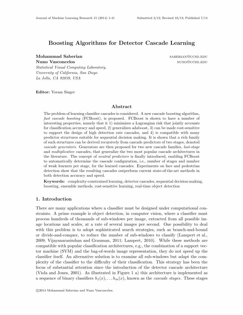
Figure 1: (a) detector cascade and (b) examples of weak learners used for face detection(Viola and Jones, 2001).

have increasing complexity, ranging from a few machine operations for h1(x) to extensivecomputation for hm(x). An example x is declared a target by the cascade if and only ifit is declared a target by all its stages. Since the overwhelming majority of sub-windowsin an image do not contain the target object, a very large portion of the image is usuallyrejected by the early cascade stages. This makes the average detection complexity quitelow. However, because the later stages can be arbitrarily complex, the cascade can havevery good classification accuracy. This was convincingly demonstrated by using the cascadearchitecture to design the first real-time face detector with state-of-the-art classification ac-curacy (Viola and Jones, 2001). This detector has since found remarkable practical success,and is today popular in applications of face detection involving low-complexity processors,such as digital cameras or cell phones.

In the method of Viola and Jones (2001), cascade stages are designed sequentially, bysimply training each detector on the examples rejected by its predecessors. Each stageis designed by boosting decision stumps that operate on a space of Haar wavelet fea-tures, such as those shown in Figure 1-b). Hence, each stage is a linear combination ofweak learners, each consisting of a Haar wavelet and a threshold. This has two appeal-ing properties. First, because it is possible to evaluate each Haar wavelet with a fewmachine operations, cascade stages can be very efficient. Second, it is possible to con-trol the complexity of each stage by controlling its number of weak learners. However,while fast and accurate, this detector is not optimal under any sensible definition of cas-cade optimality. For example, it does not address the problems of 1) how to automat-ically determine the optimal cascade configuration, e.g., the numbers of cascade stagesand weak learners per stage, 2) how to design individual stages so as to guarantee opti-mality of the cascade as a whole, or 3) how to factor detection speed as an explicit vari-able of the optimization process. These limitations have motivated many enhancements tothe various components of cascade design, including 1) new features (Lienhart and Maydt,2002; Dalal and Triggs, 2005; Pham et al., 2010; Dollar et al., 2009), 2) faster feature se-lection procedures (Wu et al., 2008; Pham and Cham, 2007), 3) post-processing proceduresto optimize cascade performance (Lienhart and Maydt, 2002; Luo, 2005; Sun et al., 2004),4) extensions of adaboost for improved design of the cascade stages (Viola and Jones,2002; Masnadi-Shirazi and Vasconcelos, 2007; Sochman and Matas, 2005; Schneiderman,2004; Li and Zhang, 2004; Tuzel et al., 2008), 5) alternative cascade structures (Xiao et al.,

2

Boosting Detector Cascade

2003; Bourdev and Brandt, 2005; Xiao et al., 2007; Sochman and Matas, 2005), and 6)joint, rather than sequential stage design (Dundar and Bi, 2007; Lefakis and Fleuret, 2010;Sochman and Matas, 2005; Bourdev and Brandt, 2005). While these advances improvedthe performance, the optimal design of a whole cascade is still an open problem. Mostexisting solutions rely on assumptions, such as the independence of cascade stages, that donot hold in practice.

In this work, we address the problem of automatically learning both the configurationand the stages of a high detection rate detector cascade, under a definition of optimalitythat accounts for both classification accuracy and speed. This is accomplished with the fastcascade boosting (FCBoost) algorithm, an extension of adaboost derived from a Lagrangianrisk that trades-off detection performance and speed. FCBoost optimizes this risk withrespect to a predictor that complies with the sequential decision making structure of thecascade architecture. These predictors are called cascade predictors, and it is shown that arich family of such predictors can be derived recursively from a set of cascade generator func-tions, which are cascade predictors of two stages. Boosting algorithms are derived for twoelements of this family, last-stage and multiplicative cascades. These are shown to generalizethe cascades of embedded (Xiao et al., 2003; Bourdev and Brandt, 2005; Xiao et al., 2007;Sochman and Matas, 2005; Masnadi-Shirazi and Vasconcelos, 2007; Pham et al., 2008) orindependent (Viola and Jones, 2001; Schneiderman, 2004; Brubaker et al., 2008; Wu et al.,2008; Shen et al., 2011, 2010) stages commonly used in the literature. The search for thecascade configuration is naturally integrated in FCBoost by the introduction of neutral pre-dictors. This allows FCBoost to automatically determine 1) number of cascade stages and2) number of weak learners per stage, by simple minimization of the Lagrangian risk. Theprocedure is compatible with existing cost-sensitive extensions of boosting (Viola and Jones,2002; Masnadi-Shirazi and Vasconcelos, 2007; Pham et al., 2008; Masnadi-Shirazi and Vasconcelos,2010) that guarantee cascades of high detection rate, and generalizes adaboost in a numberof interesting ways. A detailed experimental evaluation on face and pedestrian detectionshows that the resulting cascades outperform current state-of-the-art methods in both de-tection accuracy and speed.

The paper is organized as follows. Section 2 reviews the challenges of cascade learningand previously proposed solutions. Section 3 briefly reviews adaboost, the most popularstage learning algorithm, and proposes its generalization for the learning of detector cas-cades. Section 4 studies the structure of cascade predictors, introducing the concept ofcascade generators. Two generators are then proposed, from which two cascade families(last-stage and multiplicative) are derived. The search for the cascade configuration is thenstudied in Section 5. In this section the Lagrangian extension of the cascade boosting algo-rithm is introduced, so as to account for detector complexity in the cascade optimization,and a procedure for the automatic addition of cascade stages during boosting is developed,using neutral predictors. All these contributions are consolidated into the FCBoost algo-rithm in Section 6, whose specialization to last-stage and multiplicative cascades is shownto generalize the two main previous approaches to cascade design. A number of interestingproperties of the algorithm are also discussed, and a cost-sensitive extension is derived.Finally, an experimental evaluation is presented in Section 7 and some conclusions drawn inSection 8. An early version of this work was presented in NIPS (Saberian and Vasconcelos,2010).

3


2. Prior Work

A large literature on detector cascade learning has emerged over the past decade. In thissection, we briefly review the main problems in this area and their current solutions.

2.1 The Problems of Cascade Learning

As illustrated in Figure 1, a cascaded detector is a sequence of detector stages. The aimis to detect instances from a target class. Examples from this class are denoted positiveswhile all others are denoted negatives. An example rejected, i.e., declared a negative, byany stage is rejected by the cascade. Examples classified as positives are propagated tosubsequent stages. To be computationally efficient, the cascade must use simple classi-fiers in the early stages and complex ones later on. Under the procedure proposed byViola and Jones (2001), the cascade designer must first select a number of stages and thetarget detection/false-positive rate for each stage. A high detection rate is critical, since im-properly rejected positives cannot be recovered. The false-positive rate is less critical, sincethe cascade false-positive rate can be decreased by addition of stages, although at the priceof extra computation. The stages are designed with adaboost. The target detection rateis met by manipulating the stage threshold, and the target false-positive rate by increasingthe number of weak learners. This frequently leads to an exceedingly complex learningprocedure. One difficulty is that the optimal cascade configuration (number of stages andstage target rates) is unknown. We refer to this as the cascade configuration problem. Whilesome configurations have evolved by default, e.g., 20 stages, with a detection rate of 99.5%and a false-positive rate of 50%, there is nothing special about these values. This problemis compounded by the fact that, for late stages where negative examples are close to theclassification boundary, it may be impossible to meet the target rates. In this case, thedesigner must backtrack (redesign some of the previous stages). Frequently, various itera-tions of parameter tuning are needed to reach a satisfactory cascade. Since each iterationrequires boosting over a large set of examples and features, the process can be tedious andtime consuming. We refer to this as the design complexity problem.

Even when a cascade is successfully designed, the process has no guarantees of opti-mal classification performance. One problem is that, while computationally efficient, theHaar wavelet features lacks discriminant power for many applications. This is the fea-ture design problem. This problem is frequently compounded by lack of convergence ofadaboost. Note that while adaboost is consistent (Bartlett and Traskin, 2007), there areno guarantees that a classifier with small number of boosting iterations, e.g., early stagesof a cascade, will produce classifiers that generalize well. We refer to this as the conver-gence problem. This problem is magnified by the mismatch between the adaboost risk,which penalizes misses/false-positives equally, and the asymmetry of the target detectionand false-positive rates used in practice. Although a stage can always meet the targetdetection rate by threshold manipulation, the resulting false-positive rate can be stronglysub-optimal (Masnadi-Shirazi and Vasconcelos, 2010). In general, better performance isobtained with asymmetric learning algorithms, that optimize the detector explicitly for thetarget detection rate. This is the cost-sensitive learning problem. Besides classificationoptimality, the learned cascade is rarely the fastest possible. This is not surprising, sincespeed is not an explicit variable of the cascade optimization process. While the specification

4


of stage false-positive rates can be used to shuffle computation between stages, there is noway to predict the amount of computation corresponding to a particular rate. This is thecomplexity optimization problem.

2.2 Previous Solutions

Over the last ten years, significant research has been devoted to all of the above problems.

Feature design: Viola and Jones introduced a very efficient set of Haar wavelets(Viola and Jones, 2001). They showed that these features could be extracted, with a fewoperations, from an integral image (cumulative image sum). While all features in the originalHaar set were axis-aligned, it is possible to extent it for 45 rectangles, (Lienhart and Maydt,2002). Similarly, several authors pursued extensions to other orientations (Carneiro et al.,2008; Du et al., 2006; Messom and Barczak, 2006). More recently, this has been extended tocompute integral images over arbitrary polygonal regions (Pham et al., 2010). Beyond thesefeatures, integral images can also be used to efficiently compute histograms (Porikli, 2005).This reduces to quantizing the image into a set of channels (associated with the histogrambins) and computing an integral image per channel. For example, a computationally efficientversion of the HOG descriptor (Dalal and Triggs, 2005) was then developed and used todesign a real-time pedestrian detector cascade (Zhu et al., 2006). More recently, this ideahas been extended to multiple other channels (Dollar et al., 2009). Finally, extensionshave been developed for more general statistical descriptors, e.g., the covariance features(Tuzel et al., 2008). While the algorithms proposed in this work support any of thesefeatures, we adopt the Haar set (Viola and Jones, 2001). This is mostly for consistencywith the cascade learning literature, where Haar wavelets are predominant.

Design of stage classifiers: A number of enhancements to the stage learning methodof Viola and Jones detector have been proposed specifically to address the problems ofconvergence rate, cost-sensitive learning, and training complexity. One potential solutionto the convergence problem is to adopt recent extensions of adaboost, which converge withsmaller numbers of weak learners. Since adaboost is a greedy feature selection algorithm,the effective number of weak learners can be reduced by using forward-backward featureselection procedures (Zhang, 2011) or reweighing weak learners by introduction of sparsityconstraints in the optimization (Collins et al., 2002; Duchi and Singer, 2009). This resultsin more accurate classification with less weak learners, i.e., a faster classifier. While thesealgorithms have not been used in the cascade learning literature, several authors haveused similar ideas to improve stage classifiers. For example, augmenting adaboost with afloating search that eliminates weak learners of small contribution to classifier performance(Li and Zhang, 2004) or by using linear discriminant analysis (LDA) (Shen et al., 2011,2010). Moreover, by interpreting the boosted classifier as a hyperplane in the space ofweak learner outputs, several authors have shown how to refine the hyperplane normal soas to maximize class discrimination. Procedures that recompute the weight of each weaklearner have been implemented with SVMs (Xiao et al., 2003), variants of LDA (Wu et al.,2008; Shen et al., 2011, 2010), and non-linear feature transformations (Schneiderman, 2004).The hyperplane refinement usually optimizes classification error directly, rather than theexponential loss of adaboost, further improving the match between learning objective andclassification performance. Finally, faster convergence is usually possible with different weak

5


learners, e.g., linear SVMs (Zhu et al., 2006) or decision trees of depth two (Dollar et al.,2009), and boosting algorithms such as realboost or logitboost (Sochman and Matas, 2005;Schneiderman, 2004; Li and Zhang, 2004; Tuzel et al., 2008).

Beyond classification performance, some attention has been devoted to design complex-ity. Since the bulk of the learning time is spent on weak learner selection, low-complexitymethods have been proposed for this. For example, it is possible to trade off memory forcomputational efficiency (Wu et al., 2008) or to model Haar wavelet responses as Gaus-sian variables, whose statistics can be computed efficiently (Pham and Cham, 2007). Whilespeeding up the design of each stage, these methods do not eliminate all aspects of thresholdtuning, stage backtracking, etc. It could be argued that this is the worst component of designcomplexity, since these operations require manual supervision. A number of enhancementshave been proposed in this area. While Viola and Jones proposed stage-specific thresholdadjustments (Viola and Jones, 2001), it is possible to formulate threshold adjustments as ana-posteriori optimization of the whole cascade (Luo, 2005; Sun et al., 2004). These methodsare hampered by the limited effectiveness of threshold adjustments when stage detectorshave poor ROC performance (Masnadi-Shirazi and Vasconcelos, 2010). Better performanceis usually achieved with cost-sensitive extensions of boosting, which optimize a cost-sensitiverisk directly (Viola and Jones, 2002; Masnadi-Shirazi and Vasconcelos, 2007; Pham et al.,2008). More recently, Masnadi-Shirazi et al. proposed Bayes consistent cost-sensitive ex-tensions of adaboost, logitboost, and realboost (Masnadi-Shirazi and Vasconcelos, 2010).These algorithms were shown to substantially improve the false-positive performance ofcascades of high detection rate (Masnadi-Shirazi and Vasconcelos, 2007). These could becombined with the methods which devise a predictor of the optimal false positive and de-tection rate for each stage, from statistics of the previous stages, so as to design a cascadeof cost-sensitive stages automatically (Brubaker et al., 2008; Dundar and Bi, 2007).

Cascade configuration: Most of the above enhancements assume a known cascadeconfiguration and sequential stage learning. This is a suboptimal design strategy and the as-sumed cascade configuration may not be attainable in practice. An alternative is to adoptcascades of embedded stages where each stage is the starting point for the design of thenext (Xiao et al., 2003; Bourdev and Brandt, 2005; Xiao et al., 2007; Sochman and Matas,2005; Masnadi-Shirazi and Vasconcelos, 2007; Pham et al., 2008). The main advantage ofthis structure is that the whole cascade can be designed with a single boosting run, andadding exit points to a standard classifier ensemble. This also minimizes the convergencerate problems of individual stage design. Using Wald’s theory of sequential decision mak-ing, it is possible to derive a method for learning embedded stages (Sochman and Matas,2005). While attempting to optimize the whole cascade, these approaches do not fullyaddress the configuration problem. Some simply add an exit point per weak learner(Masnadi-Shirazi and Vasconcelos, 2007; Xiao et al., 2007; Sochman and Matas, 2005), whileothers use post-processing (Bourdev and Brandt, 2005; Xiao et al., 2003) or pre-specifieddetection and false-positive rates (Pham et al., 2008) to determine exit point locations.More recently, it is proposed to learn all stages simultaneously, by modeling a cascade asthe product, or logical “AND”, of its stages (Lefakis and Fleuret, 2010; Raykar et al., 2010).

Overall, despite substantial progress, no method addresses all problems of cascade learn-ing. Since few approaches explicitly optimize the cascade configuration, fewer among theserely on cost-sensitive learning, and no method optimizes detection speed explicitly, cas-

6


cade learning can require extensive trial and error. This can be quite expensive from acomputational point of view and leads to a tedious design procedure, which can producesub-optimal cascades. In the following sections we propose an alternative framework, whichis fully automated and jointly determines 1) the number of cascade stages, 2) the numberof weak learners per stage, and 3) the predictor of each stage, by minimizing a Lagrangianrisk that is cost-sensitive and explicitly accounts for detection speed.

3. An Extension of Adaboost for the Design of Classifier Cascades

We start with a brief review of boosting.

3.1 Boosting

A binary classifier h : X → −1, 1 maps an example x into a class label y(x). A learningalgorithm seeks the classifier of minimum probability of error, PX(h(x) 6= y(x)), in thespace of binary mappings

H = h|h : X → −1, 1 .

Since H is not convex and h ∈ H not necessarily differentiable, this is usually done byrestricting the search to mappings of the form

h(x) = sign[f(x)],

where f : X → R, is a predictor. The goal is then to learn the optimal f(x) in a set ofpredictors

F = f |f : X → R .

This is the predictor which minimizes the classification risk, RE : F → R,

RE [f ] = EX,Y L(y(x), f(x)) ≃1

|St|

∑

i

L(yi, f(xi)), (1)

where L : +1,−1 × R → R is a loss function, and St = (x1, y1), . . . , (xn, yn) is a set oftraining examples xi of labels yi.

Boosting algorithms are iterative procedures that learn f as a combination of simplepredictors, known as weak learners, from a set G = g1(x), . . . , gn(x) ⊂ F. The optimalcombination is the solution of

minf(x) RE [f ]

s.t : f(x) ∈ span(G).(2)

Each boosting iteration reweights the training set and adds the weak learner of lowestweighted error rate to the weak learner ensemble. When G is rich enough, i.e., contains apredictor with better than chance-level weighted error rate for any distribution over trainingexamples, the boosted classifier can be arbitrarily close to the minimum probability of errorclassifier (Freund and Schapire, 1997). For most problems of practical interest, G is anovercomplete set and the solution of (2) can have many decompositions in span(G). In thiscase, sparser decompositions are likely to have better performance, i.e., faster computation

7


and better generalization. Boosting can be interpreted as a greedy forward feature selectionprocedure to find such sparse solutions.

Although the ideas proposed in this work can be combined with most boosting al-gorithms, we limit the discussion to adaboost (Freund and Schapire, 1997). This is analgorithm that learns a predictor f by minimizing the risk of (1) when L is the negativeexponential of the margin y(x)f(x)

L(y(x), f(x)) = e−y(x)f(x). (3)

This is known as the exponential loss function (Schapire and Singer, 1999).

The boosting algorithms proposed in this paper are inspired by the statistical view ofadaboost (Mason et al., 2000; Friedman, 1999). Under this view, each iteration of boostingcomputes the functional derivatives of the risk along the directions of the weak learnersgk(x), at the current solution f(x). This can be written as

< δRE [f ], g > =d

dǫRE [f + ǫg]

∣

∣

∣

∣

ǫ=0

=1

|St|

∑

i

[

d

dǫe−yi(f(xi)+ǫg(xi))

]

ǫ=0

= −1

|St|

∑

i

yiwig(xi), (4)

where yi = y(xi) and

wi = w(xi) = e−yif(xi), (5)

is the weight of example xi. The latter measures how well xi is classified by the currentpredictor f(x). The predictor is then updated by selecting the direction (weak learner) ofsteepest descent

g∗(x) = argmaxg∈G

< −δRE [f ], g >

= argmaxg∈G

1

|St|

∑

i

yiwig(xi), (6)

and computing the optimal step size along this direction

α∗ = argminα∈R

RE [f + αg∗]. (7)

While the optimal step size has a closed form for adaboost (Freund and Schapire, 1997), itcan also be found by a line search. The predictor is finally updated according to

f(x) = f(x) + α∗g∗(x), (8)

and the procedure iterated, as summarized in Algorithm 1.

8


Algorithm 1 adaboost

Input: Training set St = (x1, y1), . . . , (xn, yn), where yi ∈ 1,−1 is the class label ofexample xi, and number of iterations N .Initialization: Set f(x) = 0.for t = 1 to N do

Compute < −δRE [f ], g > for all weak learners using (4).Select the best weak learner g∗(x) using (6).Find the optimal step size α∗ along g∗(x) using (7).Update f(x) = f(x) + α∗g∗(x).

end for

Output: decision rule: sign[f(x)]

3.2 Cascade Boosting

In this work, we consider the question of whether boosting can be extended to learn adetector cascade. We start by introducing some notation. As shown in Figure 1-a), aclassifier cascade is a binary classifier H(x) ∈ H implemented as a sequence of classifiers

hi(x) = sgn[fi(x)] i = 1, . . . ,m, (9)

where the predictors fi(x) can be any real functions, e.g., linear combinations of weaklearners. The cascade implements the mapping H : X → −1, 1 where

H(x) = Hm[h1, . . . , hm](x) =

−1 if ∃ k : hk(x) < 0+1 otherwise,

(10)

and Hm[h1, . . . , hm] is a classifier cascading (CC) operator, i.e., a functional mapping Hm :Hm → H of the stage classifiers h1, . . . , hm into the cascaded classifier H.1

Similarly, it is possible to define a cascade predictor F (x) for H(x), i.e., a mappingF : X → R such that

H(x) = sign[F (x)], (11)

whereF (x) = Fm[f1, . . . , fm](x), (12)

and Fm : Fm → F is a predictor cascading (PC) operator, i.e., a functional mapping of thestage predictors f1, . . . , fm into the cascade predictor F . We will study the structure of thisoperator in Section 4. For now, we consider the problem of learning a cascade, given thatthe operator Fm is known.

To generalize adaboost to this problem it suffices to use the predictor F (x) in theexponential loss of (3) and solve the optimization problem

minm,f1,...fm RE [F ] =1

|St|

∑

i e−yiF (xi)

s.t : F (x) = Fm[f1, . . . , fm](x)∀i fi(x) ∈ span(G)

(13)

1. The notation Hm[h1, . . . , hm](x) should be read as: the value at x of the image of (h1, . . . , hm) under

operator Hm.

9


by gradient descent in span(G). The main difference with respect to adaboost is that, sinceany of the cascade stages can be updated, multiple gradient steps are possible per iteration.The directional gradient for updating the predictor of the kth stage is

< δRE [F ], g >k=d

dǫRE [F

m[f1, . . . fk + ǫg, . . . fm]]

∣

∣

∣

∣

ǫ=0

=1

|St|

∑

i

[

d

dǫe−yiFm[f1,...fk+ǫg,...fm](xi)

]

ǫ=0

=1

|St|

∑

i

(−yi)e−yiFm[f1,...fm](xi)

[

d

dǫFm[f1, . . . fk + ǫg, . . . fm]

]

ǫ=0

(xi)

= −1

|St|

∑

i

yiw(xi)bk(xi)g(xi), (14)

with

w(xi) = e−yiFm[f1,...fm](xi) = e−yiF (xi) (15)

bk(xi) =d

dǫFm[f1, . . . fk + ǫg, . . . fm]

∣

∣

∣

∣

ǫ=0

(xi). (16)

The optimal descent direction for the kth stage is then

g∗k = argmaxg∈G

< −δRE [F ], g >k

= argmaxg∈G

1

|St|

∑

i

yiw(xi)bk(xi)g(xi), (17)

the optimal step size along this direction is

α∗k = argmin

α∈RRE [F

m[f1, .., fk + αg∗k, ..fm]], (18)

and the optimal stage update is

fk(x) = fk(x) + α∗g∗(x). (19)

The steps of (15), (17), and (19) constitute a functional gradient descent algorithm forlearning a detector cascade, which generalizes adaboost. In particular, the weight of (15)generalizes that of (5), reweighing examples by how well the current cascade classifies them.The weak learner selection rule of (17) differs from that of (6) only in that this weight ismultiplied by coefficient bk(xi). Finally, (19) is an additive update, similar to that of (8). Ifthe structure of the optimal cascade were known, namely how many stages it contains, thesesteps could be used to generalize Algorithm 1. It would suffice to, at each iteration t, selectthe stage k such that g∗k achieves the smallest risk in (18) and update the predictor of thatstage. This only has a fundamental difference with respect to adaboost: the introduction ofthe coefficients bk(xi) in the weak learner selection. We will see that the procedure abovecan also be extended into an algorithm that learns the cascade configuration. Since theseextensions depend on the PC operator F of (12), we start by studying its structure.

10


4. The Structure of Cascade Predictors

In this section, we derive a general form for Fm. We show that any cascade is compatiblewith an infinite set of predictors and that these can be computed recursively. This turns outto be important for the efficient implementation of the learning algorithm of the previoussection. We next consider a class of PC operators synthesized by recursive application ofa two-stage PC operator, denoted the generator of the cascade. Two generators are thenproposed, from which we derive two new cascade predictor families that generalize the twomost common cascade structures in the literature.

4.1 Cascade Predictors

From (10), a classifier cascade implements the logical-AND of the outputs of its stageclassifiers, i.e., Hm is the pointwise logical-AND of h1, . . . , hm,

Hm[h1, . . . , hm](x) = h1(x) ∧ . . . ∧ hm(x), (20)

where ∧ is the logical-AND operation. Since, from (10)-(12),

Hm[h1, . . . , hm](x) = sgn[Fm[f1, . . . , fm](x)], (21)

it follows from (9) that

sign[Fm[f1, . . . , fm](x)] = sgn[f1(x)] ∧ . . . ∧ sgn[fm(x)]. (22)

This holds if and only if

Fm[f1, . . . , fm](x) < 0 if ∃ k : fk(x) < 0Fm[f1, . . . , fm](x) > 0 otherwise.

(23)

Since (22) holds for any operator with this property, any such Fm is denoted a pointwisesoft-AND of its arguments. In summary, while a cascade implements the logical-ANDof its stage decisions, the cascade predictor implements a soft-AND of the correspondingstage predictions. Note that there is an infinite number of soft-AND operators which willimplement the same logical-AND operator, once thresholded according to (21). This makesthe set of cascade predictors much richer than that of cascades.

4.2 Recursive Implementation

For any m, it follows from (20) and the associative property of the logical-AND that

Hm[h1, . . . , hm] =

H2[h1, h2], m = 2H2

[

h1,Hm−1[h2, . . . , hm]

]

m > 2.(24)

A similar decomposition holds for the soft-AND operator of (23), since

sgn [Fm[f1, . . . , fm](x)] =

sgn[

F2[f1, f2](x)]

, m = 2sgn

[

F2[

f1,Fm−1[f2, . . . , fm]

]

(x)]

m > 2.(25)

The main difference between the two recursions is that, while there is only one logical-ANDH2[f1, f2], an infinite set of soft-AND operators F2[f1, f2] can be used in (25). In fact, it is

11


possible to use a different operator F2 at each level of the recursion, i.e., replace F2 by F2m,

to synthesize all possible sequences of soft-AND operators F imi=2 for which the left-handside of (25) is the same. For simplicity, we only consider soft-AND operators of the formof (25) in this work.

The recursions above make it possible to derive a recursive decomposition of both thecascade and the sign of its predictor. In particular, defining

Hk(x) = Hm−k+1[hk, . . . , hm](x),

(24) leads to the cascade recursion

Hk(x) =

hm(x), k = m

H2 [hk, Hk+1] (x), 1 ≤ k < m,

with H1(x) = H(x). Similarly, for any sequence of soft-AND operators F imi=2 compatiblewith (25), defining

Fk(x) = Fm−k+1[fk, . . . , fm](x),

leads to the predictor recursion

sgn[Fk(x)] =

sgn[fm(x)], k = m

sgn[

F2 [fk, Fk+1] (x)]

, 1 ≤ k < m,(26)

with sgn[F1(x)] = sgn[F (x)]. Simplifying (26), in the remainder of this work we considerpredictors of the form

Fk(x) =

fm(x), k = m

F2 [fk, Fk+1] (x), 1 ≤ k < m.(27)

Since the core of this recursion is the two-stage predictor

G[f1, f2] = F2[f1, f2], (28)

this is denoted the generator of the cascade. We will show that the two most popular cascadearchitectures can be derived from two such generators. For each, we will then derive thecascade predictors Fk(x), the cascade boosting weights w(xi) of (15), and the coefficientsbk(xi) of (16). We start by defining some notation to be used in these derivations.

4.3 Some Definitions

Some of the computations of the following sections involve derivatives of Heaviside stepfunctions u(.), which are not differentiable. As is common in the neural network literature,this problem is addressed with the sigmoidal approximation

u(x) ≈ σ(x) =1

2(tanh(µx) + 1). (29)

The parameter µ controls the sharpness of the sigmoid. This approximation is well knownto have the symmetry σ(−x) = 1 − σ(x) and derivative σ′(x) = 2µσ(x)σ(−x). We alsointroduce the sequence of cascaded Heaviside functions

γk(x) =

1, k = 1∏

j<k u[fj(x)], k > 1,(30)

12


and cascaded rectification functions

ξk(x) =

1, k = 1∏

j<k fj(x)u[fj(x)], k > 1,(31)

where u(.) is the Heaviside step. The former generalize the Heaviside step, in the sensethat γk(x) = 1 if fj(x) > 0 for all j < k and γk(x) = 0 otherwise. The latter generalizethe half-wave rectifier, in the sense that γk(x) =

∏

j<k fj(x) if fj(x) > 0 for all j < k andγk(x) = 0 otherwise.

4.4 Last Stage Cascades

The first family of cascade predictors that we consider is derived from the generator

G1[f1, f2](x) = f1(x)u[−f1(x)] + u[f1(x)]f2(x)

=

f1(x) if f1(x) < 0f2(x) if f1(x) ≥ 0,

(32)

Using (27), the associated predictor recursion is

Fk(x) =

fm(x), k = m

fk(x)u[−fk(x)] + u[fk(x)]Fk+1(x), 1 ≤ k < m.(33)

The kth stage of the associated cascade passes example x to stage k + 1 if fk(x) ≥ 0.Otherwise, the example is rejected with prediction fk(x). Hence,

Fm[f1, . . . , fm](x) =

fj(x) if fj(x) < 0 andfi(x) ≥ 0 i = 1, . . . , j − 1

fm(x) if fi(x) ≥ 0 i = 1 . . . ,m− 1,

i.e., the cascade prediction is that of the last stage visited by the example. For this reason,the cascade is denoted a last-stage cascade.

This property makes it trivial to compute the weights w(x) of the cascade boostingalgorithm, using (15). It suffices to evaluate

w(xi) = e−yifj∗ (xi), (34)

where j∗ is the smallest k for which fk(xi) is negative and j∗ = m if there is no such k.The computation of bk(x) with (16) requires a differentiable form of Fm[f1, . . . , fm] with

13


respect to fk. This can be obtained by recursive application of (33), since

Fm[f1, . . . , fm](x) = F1(x)

= f1(x)u[−f1(x)] + u[f1(x)]F2(x)

= f1(x)u[−f1(x)] + u[f1(x)] f2(x)u[−f2(x)] + u[f2(x)]F3(x)

=

k−1∑

i=1

fi(x)u[−fi(x)]∏

j<i

u[fj(x)]

+ Fk(x)∏

j<k

u[fj(x)]

=

[

k−1∑

i=1

fi(x)u[−fi(x)]γi(x)

]

+ Fk(x)γk(x) k = 1 . . .m

=

[

k−1∑

i=1


]

+ γk(x) fk(x)u[−fk(x)] + u[fk(x)]Fk+1(x) k < m

=

[

k−1∑

i=1


]

+ γk(x) fk(x) + u[fk(x)][Fk+1(x)− fk(x)]

≈

[

k−1∑

i=1


]

+ γk(x)fk(x) + γk(x)σ[fk(x)][Fk+1(x)− fk(x)] (35)

where γk(x) are the cascaded Heaviside functions of (30) and we used the differentiableapproximation of (29) in (35). Note that neither the first term on the right-hand side of(35) nor γk or Fk+1 depend on fk. It follows from (16) that

bk(x) =

γk(x), k = m

γk(x)1 + 2µσ[fk(x)][Fk+1(x)− fk(x)]σ[−fk(x)] 1 ≤ k < m,(36)

where σ(.) is defined in (29). Given x, all these quantities can be computed with a sequenceof a forward, a backward, and a forward pass through the cascade. The initial forwardpass computes γk(x) for all k according to (30). The backward pass then computes Fk+1(x)using (33). The final forward pass computes the weight w(x) and coefficients bk(x) using(34) and (36). These steps are summarized in Algorithm 2. The procedure resembles theback-propagation algorithm for neural network training (Rumelhart et al., 1968).

4.5 Multiplicative Cascades

The second family of cascade predictors has generator

G2[f1, f2](x) = f1(x)u[−f1(x)] + u[f1(x)]f1(x)f2(x)

=

f1(x) if f1(x) < 0f1(x)f2(x) if f1(x) ≥ 0.

(37)

Using (27), the associated predictor recursion is

Fk(x) =

fm(x), k = m

fk(x)u[−fk(x)] + u[fk(x)]fk(x)Fk+1(x), 1 ≤ k < m(38)

14


Algorithm 2 Last-stage cascade

Input: Training example (x, y), stage predictors fk(x), k = 1, . . . ,m, sigmoid parameterµ.Evaluation:

Set γ1(x) = 1.for k = 2 to m do

Set γk(x) = γk−1(x)u[fk(x)].end for

Set Fm(x) = fm(x).for k = m− 1 to 1 do

Set Fk(x) = fk(x)u[−fk(x)] + u[fk(x)]Fk+1(x).end for

Learning:

Set w(x) = e−yfj∗ (x) where j∗ is the smallest k for which fk(xi) < 0 and j∗ = m if thereis no such k.for k = 1 to m− 1 do

Set bk(x) = γk(x)1 + 2µσ[fk(x)][Fk+1(x)− fk(x)]σ[−fk(x)].end for

Set bk(x) = γm(x).Output: w(x), Fk(x), bk(x)

mk=1.

and

Fm[f1, . . . , fm](x) =

∏

i≤j fi(x) if fj(x) < 0 and

fi(x) ≥ 0 i = 1..j − 1∏m

i=1 fi(x) if fi(x) ≥ 0 i = 1..m− 1.

Hence, the cascade predictor is the product of all stage predictions up-to and including thatwhere the example is rejected. This is denoted a multiplicative cascade.

The weights w(x) of the cascade boosting algorithm are

w(xi) = e−yi∏

k≤j∗ fk(xi),

where j∗ is the smallest k for which fk(xi) is negative and j∗ = m if there is no such k.The computation of bk(x) with (16) requires a differentiable form of Fm[f1, . . . , fm] with

15


respect to fk. This can be obtained by recursive application of (38), since

Fm[f1, . . . , fm](x) = F1(x)

= f1(x)u[−f1(x)] + u[f1(x)]f1(x)F2(x)

= f1(x)u[−f1(x)] + u[f1(x)]f1(x)f2(x)u[−f2(x)] + u[f2(x)]f2(x)F3(x)

=

k−1∑

i=1

fi(x)u[−fi(x)]∏

j<i

fj(x)u[fj(x)]

+ Fk(x)∏

j<k

fj(x)u[fj(x)]

=

[

k−1∑

i=1

fi(x)u[−fi(x)]ξi(x)

]

+ Fk(x)ξk(x) k = 1 . . .m

=

[

k−1∑

i=1


]

+ ξk(x) fk(x)u[−fk(x)] + u[fk(x)]fk(x)Fk+1(x) k < m

=

[

k−1∑

i=1


]

+ ξk(x)fk(x) 1 + u[fk(x)][Fk+1(x)− 1]

≈

[

k−1∑

i=1


]

+ ξk(x)fk(x) 1 + σ[fk(x)][Fk+1(x)− 1] , (39)

where ξi(x) are the rectification functions of (31) and we used (38) and the differentiableapproximation of (29) in (39). Since neither the first term on the right hand side, ξk, orFk+1 depend on fk, it follows from (16) that

bk(x) =

ξm(x), k = m

ξk(x)1 + σ[fk(x)][Fk+1(x)− 1]1 + 2µfk(x)σ[−fk(x)] 1 ≤ k < m,(40)

where σ(.) is defined in (29). Again, these coefficients can be computed with a forward, abackward, and a forward pass through the cascade, which resembles back-propagation, assummarized in Algorithm 3.

5. Learning the Cascade Configuration

Given a cascade configuration, Algorithms 2 or 3, could be combined with the algorithmof Section 3.2 to extend adaboost to the design of last-stage or multiplicative cascades,respectively. However, the cascade configuration is usually not known and must be learned.This consists of determining the number of cascade stages and the number of weak learnersper stage.

5.1 Complexity Loss

We start by assuming that the number of cascade stages is known and concentrate on thecomposition of these stages. So far, we have proposed to simply update, at each boostingiteration, the stage k with the weak learner g∗k that achieves the smallest risk in (18). Whilethis will produce cascades with good detection accuracy, there is no incentive for the cascadeconfiguration to be efficient, i.e., achieve an optimal trade-off between detection accuracy

16


Algorithm 3 multiplicative cascade

Input: Training example (x, y), stage predictors fk(x), k = 1, . . . ,m, sigmoid parameterµ.Evaluation:

Set ξ1 = 1.for k = 2 to m do

Set ξk(x) = ξk−1(x)fk(x)u[fk(x)].end for

Set Fm(x) = fm(x).for k = m− 1 to 1 do

Set Fk(x) = fk(x)u[−fk(x)] + u[fk(x)]fk(x) F k+1(x).end for

Learning:

Set w(x) = e−y∏

k≤j∗ fk(x) where j∗ is the smallest k for which fk(xi) < 0 and j∗ = m ifthere is no such k.for k = 1 to m− 1 do

Set bk(x) = ξk(x)1 + σ[fk(x)][Fk+1(x)− 1]1 + 2µfk(x)σ[−fk(x)].end for

Set bm(x) = ξm(x).Output: w(x), Fk(x), bk(x)

mk=1.

and classification speed. To guarantee such a trade-off it is necessary to search for themost accurate detector under a complexity constraint. This can be done by minimizing theLagrangian

L[F ] = RE [F ] + ηRC [F ], (41)

where F (x) and RE [F ] are the cascade predictor and classification risk of (13), respectively,

RC [F ] = EX|Y LC(F, x)|y(x) = −1 ≃1

|S−t |

∑

xi∈S−t

LC(F, xi),

is a complexity risk and η a Lagrange multiplier that determines the trade-off betweenaccuracy and computational complexity. RC [F ] is the empirical average of a computa-tional loss LC(F, x), which reflects the number of machine operations required to evaluateF (x) = Fm[f1, . . . , fm](x), over the set S−

t of negatives in St. The restriction to negativeexamples is not necessary but common in the classifier cascade literature, where computa-tional complexity is usually defined as the average computation required to reject negativeexamples. This is mostly because positives are rare and contribute little to the overallcomputation.

As is the case for the classification risk, where the loss of (3) is an upper bound onthe margin and not the margin itself, the computational loss LC [F ] is a surrogate for thecomputational cost C(F, x) of evaluating the cascade prediction F (x) for example x. Usingthe predictor recursions of Section 4.2, this cost can itself be computed recursively. Since,by definition of cascade, example x is either rejected by the predictor fk of stage k or passed

17


to the remaining stages,

C(Fk, x) =

Ω(fk) + u[fk(x)]C(Fk+1, x), k < m

Ω(fm), k = m,(42)

where Fk(x) is as defined in (27) and Ω(fk) is the computational cost of evaluating stage k.Defining C(Fm+1, x) = 0, it follows that

C(F, x) = Ω(f1) + u[f1(x)]C(F2, x)

= Ω(f1) + u[f1(x)][Ω(f2) + u[f2(x)]C(F3, x)]

=

k−1∑

i=1

Ω(fi)∏

j<i

u[fj(x)]

+ C(Fk, x)∏

j<k

u[fj(x)]

=

[

k−1∑

i=1

Ω(fi)γi(x)

]

+Ω(fk)γk(x) + u[fk(x)]C(Fk+1, x)γk(x)

= δk(x) + Ω(fk)γk(x) + θk(x)u[fk(x)], (43)

where γi(x) are the cascaded Heaviside functions of (30) and

δk(x) =k−1∑

i=1

Ω(fi)γi(x),

θk(x) = C(Fk+1, x)γk(x). (44)

This relates the cascade complexity to the complexity of the kth stage, Ω(fk). The surrogatecomputational loss LC [F, x] is inspired by the surrogate classification loss of adaboost, whichupper bounds the zero-one loss u[−yf(x)] by the exponential e−yf(x). Using the boundu[f(x)] ≤ ef(x) on (43) leads to

LC [F, x] = δk(x) + Ω(fk)γk(x) + θk(x)efk(x),

and the computational risk

RC [F ] =1

|S−t |

∑

xi∈S−t

δk(xi) + Ω(fk)γk(xi) + θk(xi)efk(xi). (45)

To evaluate this risk, it remains to determine the computational cost Ω(fk) of thepredictor of the kth cascade stage. Since fk(x) =

∑

l αlgl(x), gl ∈ G, is a linear combinationof weak learners, we define

Ω(fk) =∑

l

Ω(gl). (46)

Let W(fk) ⊂ G be the set of weak learners, gl, that appear in (46). In this work, we restrictour attention to the case where all gl have the same complexity and Ω(fk) is proportionalto |W(fk)|. This is the most common scenario in computer vision problems, such as facedetection, where all weak learners are thresholded Haar wavelet features (Viola and Jones,2001) and have similar computational cost. We will, however, account for the fact that

18


there is no cost in the repeated evaluation of a weak learner. For this, W(fk) is split intotwo sets. The first, O(fk), contains the weak learners used in some earlier cascade stagefj , j ≤ k. Since the outputs of these learners can be kept in memory, they require minimalcomputation (multiplication by αl and addition to cumulative sum). The second is the setN (fk) of weak learners unused in prior stages. The computational cost of fk is then

Ω(fk) = |N (fk)|+ λ|O(fk)|, (47)

where λ < 1 is the ratio of computation required to evaluate a used vs. new weak learner.This implies that when updating the kth stage predictor

Ω(fk + ǫg) = Ω(fk) + ρ(g, fk),

with

ρ(g, fk) =

λ if g ∈ O(fk)1 if g ∈ N (fk).

(48)

5.2 Boosting with Complexity Constraints

Given the computational risk of (45), it is possible to derive a boosting algorithm thataccounts for cascade complexity. We start by deriving the steepest descent direction of theLagrangian of (41), with respect to stage k

< −δL[F ], g >k = < −δ (RE [F ] + ηRC [F ]) , g >k

= < −δRE [F ], g >k +η < −δRC [F ], g >k .

The first term is given by (14), the second requires the descent direction with respect tothe complexity risk RC [F ]. Using (45),

< δRC [F ], g >k=d

dǫRC(F

m[f1, .., fk + ǫg, ..fm])

∣

∣

∣

∣

ǫ=0

=1

|S−t |

∑

i

ysid

dǫLC [Fm[f1, .., fk + ǫg, ..fm], xi]

∣

∣

∣

∣

ǫ=0

=1

|S−t |

∑

i

ysid

dǫ

[

δk(xi) + [Ω(fk) + ρ(fk, g)]γk(xi) + θk(xi)efk(xi)+ǫg(xi)

]

∣

∣

∣

∣

ǫ=0

=1

|S−t |

∑

i

ysiψk(xi)θk(xi)g(xi), (49)

where ysi = I(yi = −1), I(x) is the indicator function, θk(xi) as in (44) and

ψk(xi) = efk(xi). (50)

Finally, combining (14) and (49),

< −δL[F ], g >k =∑

i

(

yiw(xi)bk(xi)

|St|− η

ysiψk(xi)θk(xi)

|S−t |

)

g(xi), (51)

19


Algorithm 4 BestStageUpdate

Input: Training set St, trade-off parameter η, cascade [f1, . . . , fm], index k of the stageto update, sigmoid parameter µ.for each pair (xi, yi) in St doCompute w(xi), bk(xi), Fk(xi) e.g., using Algorithm 2 for last-stage or Algorithm 3 formultiplicative cascades.Compute θk(xi), ψk(xi) with (44) and (50).

end for

Find the best update (α∗k, g

∗k(x)) for the k

th stage using (51)-(54).Output: α∗

k, g∗k(x)

where w(xi) = e−yiF (xi) and bk(xi) is given by (36) for last-stage and by (40) for multiplica-tive cascades.

It should be noted that, although (51) does not depend on ρ(fk, g), the complexity ofthe optimal weak learner g∗ affects the computational risk in (45) and thus the magnitudeof the steepest descent step. To account for this, we find the best update for fk in twosteps. The first step searches for the best update within O(fk) and N (fk)

g∗1,k = arg maxg∈O(fk)

< −δL[F ], g >k (52)

g∗2,k = arg maxg∈N (fk)

< −δL[F ], g >k, (53)

and computes the corresponding optimal steps sizes

α∗j,k = argmin

α∈RL[Fm[f1, ..fk + αgj,k, ..fm]], (54)

for j = 1, 2. The second step chooses the update that most reduces L[F ] as the best updatefor the kth stage. The overall procedure is summarized in Algorithm 4. Using this procedureto cycle through all cascade stage updates within each iteration of the algorithm of Section3.2 and selecting the one that most reduces L[F ] produces an extension of adaboost forcascade learning that optimizes the trade-off between detection accuracy and complexity.

5.3 Growing a Detector Cascade

So far, we have assumed that the number of cascade stages is known. Since this is usuallynot the case, there is a need for a procedure that learns this component of the cascadeconfiguration. In this work, we adopt a greedy strategy, where cascade stages are addedby the boosting algorithm itself, whenever this leads to a reduction of the risk. It is as-sumed that a new stage, or predictor g, can only be added at the end of the existingcascade, i.e., transforming a m-stage predictor Fm[f1, . . . , fm](x) into a m+1-stage predic-tor Fm+1[f1, . . . , fm, g](x). This is consistent with current cascade design practices, wherestages are appended to the cascade when certain heuristics are met.

The challenge of a risk-minimizing formulation of this process is to pose the addition ofa new stage as a possible gradient step. Recall that, at each iteration of a gradient descentalgorithm, the current solution, vt, is updated by

vt+1 = vt + αv,

20


where v is the gradient update and α is step size found by a line search. An immediateconsequence is that, if no update is taken in an iteration, i.e., α = 0 or v = 0, the value of theobjective function should remain unaltered. For the proposed cascade boosting algorithmsthis condition is not trivial to guarantee when a new stage is appended to the currentcascade. For example, choosing g(x) = 0 may change the current solution since, in general,

Fm+1[f1, . . . , fm, 0](x) 6= Fm[f1, . . . , fm](x).

To address this problem, we introduce the concept of neutral predictors. A stage predictorn(x) : X → R is neutral for a cascade of predictor Fm[f1, . . . , fm] if and only if

Fm+1[f1, . . . , fm, n](x) = Fm[f1, . . . , fm](x). (55)

If such a neutral predictor exists, then it is possible to grow a cascade by defining the newstage as

fm+1(x) = n(x) + g(x),

where g(x) is the best update found by gradient descent. In this case, it follows from (55)that a step of g(x) = 0 will leave the cascade risk unaltered. Given a cascade generator, apredictor n that satisfies (55) can usually be found with (28), i.e., it suffices that n satisfies

fm(x) = G[fm, n](x), (56)

where G is the generator that defines the PC operator Fm. For example, from (32), theneutral predictor of a last-stage cascade must satisfy

fm(x) = fm(x)u[−fm(x)] + u[fm(x)]n(x),

a condition met byn(x) = fm(x). (57)

Similarly, from (37), the neutral predictor of a multiplicative cascade must satisfy

fm(x) = fm(x)u[−fm(x)] + u[fm(x)]fm(x)n(x),

which is met byn(x) = 1. (58)

These neutral predictors are also computationally efficient. In fact, (57) and (58) addno computation to the evaluation of predictor fm+1(x), i.e., to the computation of g(x)itself. This is obvious for (58) which is a constant, and follows from the fact that fm(x)has already been computed in stage m for (57). This computation can simply be reused atstage m+ 1 with no additional cost. Hence, for both models

C(Fm+1[f1, . . . , fm, n], x) = C(Fm[f1, . . . , fm], x),

andL[Fm+1[f1, . . . , fm, n]] = L[Fm[f1, . . . , fm]].

In summary, the addition of stages does not require special treatment in the proposedcascade learning framework. It suffices to append a neutral predictor to the cascade andfind the best update for this new stage. If this reduces the objective function of (41) furtherthan updating other stages, the new stage is automatically created and appended to thecascade. In this way, the cascade grows organically, as a side effect of the risk optimization,and there is no need for heuristics.

21


Algorithm 5 FCBoost

Input: Training set S = (x1, y1) . . . , (xn, yn), trade-off parameter η, sigmoid parameterµ, and number of iterations N .Initialization: Set m = 0 and f1(x) = n(x), e.g., using (57) for last-stage and (58) formultiplicative cascade.for t = 1 to N do

for k = 1 to m do

(α∗k, g

∗k) = BestStageUpdate(S, η, [f1, ...fm], k, µ).

end for

(α∗m+1, g

∗m+1) = BestStageUpdate(S, η, [f1, ...fm+1],m+ 1, µ).

for k = 1 to m do

Set L(k) = L [Fm(f1, .., fk + α∗kg

∗k, .., fm)] using (41).

end for

Set L(m+ 1) = L[

Fm+1(f1, .., fm, fm+1 + α∗m+1g

∗m+1(x))

]

using (41).

Find k∗ = argmink∈1,...,m+1 L(k).Set fk∗ = fk∗ + α∗

k∗g∗k∗ .

if k∗ = m+ 1 then

Set m = m+ 1 .Set fm+1(x) = n(x).

end if

end for

Output: decision rule: sgn[Fm(f1, . . . , fm)].

6. The FCBoost Cascade Learning Algorithm

In this section, we combine the contributions from the previous sections into the FastCascade Boosting (FCBoost) algorithm, discuss its connections with the previous literatureand some interesting properties.

6.1 FCBoost

FCBoost is initialized with a neutral predictor. At each iteration, it finds the best updateg∗k(x) for each of the cascade stages and the best stage to add at the end of the cascade.It then selects the stage k∗ whose update g∗k∗(x) most reduces the Lagrangian L[F ]. Ifk∗ is the newly added stage, a new stage is created and appended to the cascade. Theprocedure is summarized in Algorithm 5. Note that the only parameters are the multiplierη of (41), which encodes the relative importance of cascade speed vs. accuracy for thecascade designer, and the sigmoid parameter µ that controls the smoothness of the Heavisideapproximation. In our implementation we always use µ = 5. Given these parameters,FCBoost will automatically determine both the cascade configuration (number of stagesand number of weak learners per stage) and the predictor of each stage, so as to optimizethe trade-off between detection accuracy and complexity which is specified through η.

22


(a) (b)

Figure 2: Illustration of the different configurations produced by identical steps of (a) last-stage and (b) multiplicative cascade learning.

6.2 Connections to the Previous Cascade Learning Literature

FCBoost supports a large variety of cascade structures. The cascade structure is defined bythe generator G of (28), since this determines the neutral predictor n(x), according to (56),and consequently how the cascade grows as boosting progresses. The two cascade predictorsused in this work, last-stage and multiplicative, cover the two predominant cascade struc-tures in the literature. The first is the independent stage (IS) structure, (Viola and Jones,2001). In this structure stage predictors are designed independently,2 in the sense that thelearning of fk starts from an empty predictor which is irrespective of the composition ofthe previous stages, fj , j < k. The second structure is the embedded stage (ES) structurewhere predictors of consecutive stages are related by

fk+1(x) = fk(x) +w(x),

and w(x) is a single or linear combination of weak learners (Xiao et al., 2003). Underthis structure, each stage predictor contains the predictor of the previous stage, which isaugmented with some weak learners.

The connection between these structures and the models proposed in this paper can beunderstood by considering the neutral predictors of the latter. For multiplicative cascades,it follows from (58) that

fm+1(x) = 1 + αg(x),

and there is no dependence between consecutive stages. Hence, multiplicative cascades havethe IS structure. For last stage cascades, it follows from (57) that

fm+1(x) = fm(x) + αg(x).

If FCBoost always updates the last two stages, this produces a cascade with the ES struc-ture. Since FCBoost is free to update any stage, it can produce more general cascades, i.e.,a superset of the set of cascades with the ES structure.

It is interesting that two predictors with the very similar generators of (32) and (37)produce very different cascade structures. This is illustrated in Figure 2, where we considerthe cascades resulting from the following sequence of operations:

2. Note that the predictors are always statistically dependent, since the role of hi+1 is to classify examplesnot rejected by hi.

23


• iteration 1: start form an empty classifier, create first stage.

• iteration 2: add a new stage.

• iteration 3: update first stage.

• iteration 4: add a new stage.

Note that while the last-stage cascade of a) has substantial weak learner sharing acrossstages, this is not true for the multiplicative cascade of b), which is similar to the Viola andJones cascade (Viola and Jones, 2001).

6.3 Properties

Beyond these connections to the literature, FCBoost has various interesting properties as acascade boosting algorithm. First, its example weighing is very similar to that of adaboost(Freund and Schapire, 1997). A comparison of (5) and (15) shows that FCBoost reweightsexamples by how well they are classified by the current cascade. As in adaboost, thisis measured by the classification margin, but now with respect to the cascade predictor,F , (margin yF ) rather than a simple predictor f (margin yf). Second, the weak learnerselection rule of FCBoost is very similar to that of adaboost. While in (6) adaboost selectsthe weak learner g that maximizes

1

|St|

∑

i

yiwig(xi),

in (52)-(53) FCBoost selects the stage k and weak learner g that maximize

∑

i

(

yiw(xi)bk(xi)

|St|− η

ysiψk(xi)θk(xi)

|S−t |

)

g(xi). (59)

When η = 0, the only significant difference is the inclusion of bk(xi) in (59). To understandthe role of this term note that, from (36) and (40), bk(xi) = 0 whenever γk(xi) = 0 in (30),and ξk(xi) = 0 in (31). This implies that there is at least one stage j < k such that fj(xi) <0, i.e., where xi is rejected. When this holds, bk(xi) = 0 prevents xi from influencingthe update of fk(x). This is sensible: since xi will not reach the kth stage, it should notaffect its learning. Hence, the coefficients bk(xi) can be seen as gating coefficients, whichprevent examples rejected by earlier stages from affecting the learning of stage k. If η 6= 0,a similar role is played by θk(xi) in the second term of (59) since, from (44), θk(xi) = 0whenever γk(xi) = 0. Thus, if xi is rejected by a stage j < k, its processing complexity isnot considered for any stage posterior to j. Due to the gating coefficients bk(xi) and θk(xi),FCBoost emulates the bootstrapping procedure commonly used in cascade design. This isa procedure that eliminates the examples rejected by each stage from the training set ofsubsequent stages. These examples are replaced with new false positives (Viola and Jones,2001; Sung and Poggio, 1998). While FCBoost emulates “example discarding” with thegating coefficients bk(xi) and θk(xi), it does not seek new false positives. This still requiresthe “training set augmentation” of bootstrapping.

24


A third interesting property of FCBoost is the complexity penalty (second term) of (59).From (44) and (50) this is, up to constants,

− ysi γk(xi)efk(xi)C(Fk+1, xi)g(xi).

Given example xi and cascade stage k, all factors in this product have a meaningful in-terpretation. First, since ysi γk(xi) is non-zero only for negative examples which have notbeen rejected by earlier cascade stages (j < k), it acts as a selector of the false-positivesthat reach stage k. Second, since fk(xi) measures how deeply xi penetrates the positiveside of the stage k classification boundary, efk(xi) is large for the false-positives that stagek confidently assigns to the positive class. Third, since C(Fk+1, xi) is the complexity ofprocessing xi by the stages beyond k, it measures how deeply xi penetrates the cascade,if not rejected by stage k. Finally, g(xi) is the label given to xi by weak learner g(x).Since only g(xi) can be negative, the product is maximized when g(xi) = −1, γk(xi) = 1and fk(xi) and C(Fk+1, xi) are as large as possible. Hence, the best weak learner is thatwhich, on average, declares as negatives the examples which 1) are false-positives of theearlier stages, 2) are most confidently accepted as false-positives by the current stage, and3) penetrate the cascade most deeply beyond this stage. This is intuitive, in the sense thatit encourages the selection of the weak learner that most contradicts the current cascade onits most costly mistakes.

In summary, FCBoost is a generalization of adaboost with similar example weighting,gating coefficients that guarantee consistency with the cascade structure, and a cost func-tion that accounts for classifier complexity. This encourages the selection of weak learnersthat correct the false-positives of greatest computational cost. It should be mentioned thatwhile we have used adaboost to derive FCBoost, similar algorithms could be derived fromother forms of boosting, e.g., logitboost, gentle boost (Friedman et al., 1998), KLBoost(Liu and Shum, 2003) or float boost (Li and Zhang, 2004). This would amount to replac-ing the exponential loss, (3), with other loss functions. While the resulting algorithmswould be different, the fundamental properties (example reweighing, additive updates, gat-ing coefficients) would not. We next exploit this to develop a cost-sensitive extension ofFCBoost.

6.4 Cost-Sensitive FCBoost

While positive examples rejected by a cascade stage cannot be recovered by subsequentstages, the cascade false positive rate can always be reduced through addition of stages.Hence, in cascade learning, maintaining a high detection rate across stages is more criticalthan maintaining a low false positive rate. This is difficult to guarantee with the risk of (1),which is an upper bound on the error rate, treating misses and false positives equally. Severalapproaches have been proposed to enforce asymmetry during cascade learning. One possibil-ity is to manipulate the thresholds of the various detector stages to guarantee the desired de-tection rate (Viola and Jones, 2001; Sochman and Matas, 2005; Luo, 2005). This is usuallysub-optimal, since boosting predictors are not well calibrated outside a small neighborhoodof the classification boundary (Mease and Wyner, 2008). Threshold tuning merely changesthe location of the boundary and can perform poorly (Masnadi-Shirazi and Vasconcelos,2010). An alternative is to use cost sensitive boosting algorithms (Viola and Jones, 2002;

25


Masnadi-Shirazi and Vasconcelos, 2007), derived from asymmetric losses that weigh miss-detections more than false-positives, optimizing the cost-sensitive boundary directly. Thisusually outperforms threshold tuning.

In this work we adopt the cost sensitive risk of

RcE(f) =

C

|S+t |

∑

xi∈S+t

e−yif(xi) +1− C

|S−t |

∑

xi∈S−t

e−yif(xi)

=∑

xi∈St

yci e−yif(xi), (60)

where C ∈ [0, 1] is a cost factor,

yci =C

|S+t |I(yi = 1) +

1− C

|S−t |

I(yi = −1),

I(.) the indicator function, and the relative importance of positive vs. negative examplesis determined by the ratio C

1−C(Viola and Jones, 2002). This leads to the cost-sensitive

Lagrangian

Lc[F ] = RcE [F ] +RC [F ]. (61)

A derivation similar to that of (14) can be used to show that

< δRcE [F ], g >k= −

∑

i

yiyciw(xi)bk(xi)g(xi), (62)

where w(xi) = e−yiF (xi) and bk(xi) is given by (36) for last-stage and by (40) for multiplica-tive cascades. Finally, combining (61), (62), and (49),

< −δLc[F ], g >k =∑

i

(

yiyciw(xi)bk(xi)− η

ysiψk(xi)θk(xi)

|S−t |

)

g(xi). (63)

The cost-sensitive version of FCBoost replaces (51) with (63) in (52)-(53) and L by Lc

in (54).

6.5 Open Issues

One subtle difference between adaboost and FCBoost, with η = 0, is the feasible set of theunderlying optimization problems. Rewriting the FCBoost problem of (13) as

minf RE [f ]s.t : f ∈ ΩG,

(64)

where

ΩG = f |∃f1, ...fm ∈ G such that f(x) = Fm[f1, . . . , fm](x) ∀x .

and comparing (64) to (2), the two problems differ in their feasible sets, span(G) foradaboost vs. ΩG for FCBoost. Since any f ∈ span(G) is equivalent to a one-stage cascadedpredictor, it follows that f ∈ ΩG and

span(G) ⊂ ΩG.

26


Hence, the feasible set of FCBoost is larger than that of adaboost, and FCBoost can, inprinciple, find detectors of lower risk. Hence, all generalization guarantees of adaboost hold,in principle, for cascades learned with FCBoost. There is, however, one significant difference.Since span(G) is a convex set, the optimization problem of (2) is convex whenever RE(f)is a convex function of f . This is the case for the adaboost risk, and adaboost is thusguaranteed to converge to a global minimum. However, since ΩG can be a non-convex set,no such guarantees exist for FCBoost. Hence, FCBoost can converge to a local minimum.We illustrate this with an example in Section 7.1. In general, the convexity of ΩG depends onthe PC operator Fm and the set of weak learners G. There is currently little understandingon what conditions are necessary to guarantee convexity.

7. Evaluation

In this section, we report on several experiments conducted to evaluate FCBoost. Westart with a set of experiments designed to illustrate the properties of the algorithm. Wethen report results on its use to build face and pedestrian detectors with state-of-the-artperformance in terms of detection accuracy and complexity. In all cases, the training set forface detection contained 4, 500 faces (along with their flipped replicas) and 9, 000 negativeexamples, of size 24 × 24 pixels, while pedestrian detection relied on a training set of2, 347 positive and 2, 000 negatives examples, of size 72 × 30, from the Caltech Pedestriandata set (Dollar et al., 2012). All weak learners were decision-stumps on Haar wavelets(Viola and Jones, 2001).

7.1 Effect of η

We started by studying the impact of the Lagrange multiplier η, of (41), on the accuracyvs. complexity performance of FCBoost cascades. The test set consisted of 832 faces (alongwith their flipped replicas) and 1, 664 negatives. All detectors were trained for 50 iterations.The unit computational cost was set to the cost of evaluating a new Haar feature. Thisresulted in a cost of 1

5 units for feature recycling, i.e., λ = 15 in (47). Figure 3 quantifies

the structure of the cascades learned by FCBoost with η = 0 and η = 0.04: multiplicativein a) and last-stage in b). The top plots summarize the number of features assigned toeach cascade stage, and those at the bottom the computational cost per stage. Note thatsince, from (57), the neutral predictor of the last-stage cascade is its last stage, each ofthe last-stage cascade stages benefits from the features evaluated in the previous stages.Hence, as shown in the top plot of Figure 3-b, the number of weak learners per stage ismonotonically increasing. However, because most features are recycled, the cost is stilldominated by the early stages, when η = 0. With respect to the impact of η, its is clearthat, for both structures, a small η produces short cascades whose early stages containmany weak learners. On the other hand, a large η leads to much deeper cascades, and amore uniform distribution of weak learners and computation. This is sensible, since largerη place more emphasis on computational efficiency and this requires that the early stages,which tend to be evaluated for most examples, be very efficient. Hence, long cascades witha few weak learners per stage tend to be computationally more efficient than short cascadeswith many learners per stage.

27


0 5 10 15 200

10

20

30

40

50

Stage Number

Num

ber

of F

eatu

res

η = 0

η = 0.04

0 5 10 15 20 25 300

10

20

30

40

50

Stage Number

Num

ber

of F

eatu

res

η = 0

η = 0.04

0 5 10 15 200

10

20

30

40

50

Stage Number

Cos

t of E

valu

atio

n

η = 0

η = 0.04

0 5 10 15 20 25 300

5

10

15

20

Stage NumberC

ost o

f Eva

luat

ion

η = 0

η = 0.04

(a) (b)

Figure 3: Number of features (top) and computational cost (bottom) per stage of an FC-Boost cascade: (a) multiplicative, (b) last-stage.

The accuracy vs. complexity trade-off of these cascades was compared to those of a non-cascaded adaboost detector and a cascade of embedded stages derived from this detector(Masnadi-Shirazi and Vasconcelos, 2007). This converts the detector into a cascade by in-serting a rejection point per weak learner. The resulting cascade has embedded stages whichadd a single weak learner to their predecessors and is equivalent to the chain boost cascade(Xiao et al., 2003). Figure 4 depicts the trade-off between computation and accuracy ofadaboost, chain boost, and FCBoost cascades with η ∈ [0, 0.04]. The left-most (right-most)point on the FCBoost curves corresponds to η = 0 (η = 0.04). adaboost and ChainBoostpoints were obtained by limiting the number of weak learners, with a single weak learner (fulldetector) for the right-most (left-most) point. Several observations can be made from thefigure. First, as expected, increasing the trade-off parameter η produces FCBoost cascadeswith less computation and higher error. Second, FCBoost has a better trade-off betweencomplexity and accuracy (curves closer to the origin). Third, among FCBoost models,last-stage cascades have uniformly better trade-off than their multiplicative counterparts.Since last-stage are generalized embedded cascades, this confirms previous reports on theadvantages of embedded over independent stages (Pham et al., 2008; Xiao et al., 2003). Fi-nally, it is interesting to note that, when η = 0, the Lagrangian of (41) is equivalent to theadaboost risk, i.e., FCBoost and adaboost minimize the same objective. However, due totheir different feasible sets, they can learn very different detectors (see Section 6.5). While

28


0.04 0.08 0.12 0.16 0.180

10

20

30

40

50

Error RateC

ost o

f Eva

luat

ion

AdaBoost

ChainBoost

Multiplicative

Last Stage

Figure 4: Computational cost vs. error rate of the detectors learned with adaboost, chainboost, and FCBoost with the last-stage and multiplicative structures.

adaboost FCBoost+last-stage FCBoost+multiplicative

Err. rate 4.03% 4.51% 4.15%

Eval. cost 50 11.74 42.54

Table 1: Performance comparison between adaboost and FCBoost, for η = 0.

the larger feasible set of FCBoost suggests that it should produce detectors of smaller riskthan adaboost, this did not happen in our experiments.

Table 1 summarizes the error and cost of adaboost and the two FCBoost methods forη = 0. Note that the adaboost detector has a slightly lower error. The weaker accuracy ofthe FCBoost detectors suggests that the latter does get trapped in local minima. This is,in fact, intuitive as the decision to add a cascade stage makes it impossible for the gradientdescent procedure to revert back to a non-cascaded detector. By making such a decision,FCBoost can compromise the global optimality of its solution, if the global optimum is anon-cascaded detector. Interestingly, FCBoost sometimes decides to add stages even whenη = 0 (see Figure 3). As shown in Table 1, this leads to a slightly more error-prone butmuch more efficient detector than adaboost. In summary, even without pressure to minimizecomplexity (η = 0), FCBoost may trade-off error for complexity. This may be desirable ornot, depending on the application. In the experiment of Table 1, FCBoost seems to makesensible choices. For the last-stage structure, it trades a small increase in error (0.48%) fora large decrease in computation (76.5%). For the multiplicative structure, it trades-off avery small increase in error (0.12%) for a moderate (16%) decrease in computation.

7.2 Cost-Sensitive FCBoost

We next consider the combination of FCBoost and the cost sensitive risk of (60). Sincethe advantages of cost-sensitive boosting over threshold tuning are now well established(Viola and Jones, 2002; Masnadi-Shirazi and Vasconcelos, 2010), we limit the discussion tothe effect of the cost factor C on the behavior of FCBoost cascades. Cascaded face detectorswere learned for cost factors C ∈ 0.5, 0.6, 0.7, 0.8, 0.9, 0.95, 0.99. Figure 5 a) presentsthe trade-off between detection and false positive rate for last-stage and multiplicative

29


0 0.2 0.4 0.6 0.80.84

0.88

0.92

0.96

1

False Positive Rate

Det

ectio

n R

ate

Last StageMultiplicative

0.5 0.6 0.7 0.8 0.9 12

4

6

8

10

12

C

Eva

luat

ion

Cos

t

Last StageMultiplicative

(a) (b)

Figure 5: Performance of cascades learned with cost-sensitive FCBoost, using different costfactors C. (a) ROC curves, (b) computational complexity.

cascades. In both cases, the leftmost (rightmost) point corresponds to C = 0.5 (C = 0.99).Figure 5 b) presents the equivalent plot for computational cost. Several observations canbe made. First, as expected, larger cost factors C produce detectors of higher detectionand higher false-positive rate. Second, they lead to cascades of higher complexity. Thisis intuitive since, for large cost factors, FCBoost aims for a high detection rate and isvery conservative about rejecting examples. Hence, many negatives penetrate deep intothe cascade, and computation increases. Third, comparing the curves of the last-stage andmultiplicative cascades, the former again has better performance. In particular, last-stagecascades combine higher ROC curves in Figure 5 a) with lower computational cost in Figure5 b).

7.3 Face and Pedestrian Detection

Over the last decade, there has been significant interest in the problem of real-time objectdetection from video streams. In particular, the sub-problems of face and pedestrian de-tection have been the focus of extensive research, due to the demand for face detection inlow-power consumer electronics (e.g., cameras or smart-phones) and pedestrian detectionin intelligent vehicles. In this section, we compare the performance of FCBoost cascadeswith those learned by several state of the art methods in the face and pedestrian detectionliteratures.

We start with face detection, where cascaded detectors have become predominant, com-paring FCBoost to the method of Viola and Jones (VJ) (Viola and Jones, 2001), Waldboost (Sochman and Matas, 2005) and multi-exit (Pham et al., 2008). Since extensive re-sults on these and other methods are available on the MIT-CMU test set, all detectors wereevaluated on this data set. The methods above have been shown to outperform a numberof other cascade learning algorithms (Pham et al., 2008) and, to the best of our knowledge,hold the best results in this data set. In all cases, the target detection rate was set toDT = 95%. For Wald boost, multi-exit, and VJ, the training set was bootstrapped whena new stage was added to the cascade, for FCBoost when the false positive rate droppedbelow 95%. For VJ and multi-exit cascades, which require the specification of the numberof cascade stages and a target false-positive and detection rate per stage, we used 20 stages,

30


100 200 300 400 5000.65

0.7

0.75

0.8

0.85

0.9

0.95

Number of False positives

Det

ectio

n ra

te

VJ(45.33)WaldBoost(28.80)Multi−Exit(80.73)FCBoost(11.38)

Figure 6: ROCs of various face detectors on MIT-CMU. The number in the legend is the av-erage evaluation cost, i.e., average number of features evaluated per sub-window.

and the popular strategy of setting the false positive rate to 50% and the detection rate

to D1

20

T . For FCBoost we used a last-stage cascade, since this structure achieved the bestbalance between accuracy and speed in the previous experiment. We did not attempt tooptimize η, simply using η = 0.02. The cost factor C was initialized with C = 0.99. If aftera boosting update the cascade did not meet the detection rate, C was increased to

Cnew =Cold + 1

2. (65)

This placed more emphasis on avoiding misses than false positives, and was repeated untilthe updated cascade satisfied the rate constraint. The final value of C was used as theinitial value for the next boosting update.

Figure 6 show the ROCs of all detectors. The average evaluation cost, i.e., averagenumber of features evaluated per sub-window, is shown in the legend for each method.Note that the FCBoost cascade is simultaneously more accurate and faster than those ofall other methods. For example, at 100 false positives, FCBoost has a detection rate of91% as opposed to 88% for multi-exit, 83% for VJ, and 80% for Wald boost. With regardsto computation, FCBoost is 7.1, 4, and 2.5 times faster than multi-exit, VJ, and Waldboost, respectively. Overall, when compared to the FCBoost cascade, the closest cascadein terms of detection rate (multi-exit, 3% drop) is significantly slower (7 times) and theclosest cascade in terms of detection speed (Wald boost, 2.5 times slower) has a very poordetection rate (11% smaller).

We next considered the problem of pedestrian detection, comparing results to a largeset of state-of-the-art pedestrian detectors on the Caltech Pedestrian data set (Dollar et al.,2012). In this literature, it is well known that a good representation for pedestrians mustaccount for both edge orientation and color (Dalal and Triggs, 2005; Dollar et al., 2009).Similarly to Dollar et al. (Dollar et al., 2009), we adopted an image representation based ona 10 channel decomposition. This included 3 color channels (YUV color space), 6 gradientorientation channels, and a gradient magnitude channel. In all other aspects, the cascade

31


10−3

10−2

10−1

100

101

102

.05

.10

.20

.30

.40

.50

.64

.801

false positives per image

mis

s ra

te

86% VJ(2.24)38% HOG(4.18)59% FtrMine(12.5)77% Shapelet(19.60)72% PoseInv43% MultiFtr(13.89)39% HikSvm(5.41)50% LatSvm−V1(2.55)28% LatSvm−V2(1.59)30% ChnFtrs(0.85)33% FPDW(0.15)36% Pls(55.56)23% HogLbp(16.13)23% FCBoost(0.80)36% MultiFtr+CSS(37.4)16% MultiFtr+Motion(50)

Figure 7: Accuracy curves and complexity of various pedestrian detectors on the Caltechdata set. Legend: (left) miss rates at 0.1 FPPI, (right) average time, in seconds,required to process 480× 640 frame.

architecture was as before, e.g., using Haar wavelet features and decision stumps as weaklearners, the previously used values for parameters DT , and η, etc. When compared tothe face detection experiments, the only difference is that the set of weak learners wasreplicated for each channel. At each iteration, FCBoost chose the best weak learner andthe best channel to add to the cascade predictor. The performance of the FCBoost cascadewas evaluated with the toolbox of (Dollar et al., 2012). Figure 7 compares its complexityand curve of miss-detection rate vs number of false positives per image (FPPI) to thoseof a number of recent pedestrian detectors. The comparison was restricted to the popularnear scale-large setting, which evaluates the detection of pedestrians with more than 100pixels in height. The numbers shown in the left of the legend summarize the detectionperformance by the miss rate at 0.1 FPPI. The numbers shown in the right indicated theaverage time, in seconds, required for processing a 480 × 640 video frame. Note that theevaluation is not restricted to fast detectors, including the most popular architectures forobject detection in computer vision, such as the HOG detector (Dalal and Triggs, 2005) orthe latent SVM (Felzenszwalb et al., 2010). For more information on the curves and othermethods the reader is referred to Dollar et al. (2012).

Two sets of conclusions can be derived from these results. First, they confirm the ob-servation that the FCBoost cascade significantly outperforms previous cascaded detectors.A direct comparison is in fact possible against the ChnFtrs method (Dollar et al., 2009).This work introduced the multi channel features that we adopt but uses the SoftCascade al-gorithm (Bourdev and Brandt, 2005) for cascade learning. The resulting detector is amongthe top methods on this data set, missing 30% of the pedestrians at 0.1 FPPI and using0.85 seconds to process a frame. Nevertheless, the FCBoost cascade has substantially bet-ter accuracy, missing only 23% of the pedestrians at 0.1 FPPI, and requires less time (a6% speed up). Second, the results of Figure 7 show that the FCBoost cascade is one ofthe most accurate pedestrian detectors in the literature, and significantly faster than the

32


detectors of comparable accuracy. In fact, only two detectors have been reported to achieveequivalent or lower miss rates. The Hog-Lbp detector (Wang et al., 2009) has the samemiss rate (23% at 0.1 FPPI) but is 20 times slower. The MultiFtr+Motion (Walk et al.,2010) detector has a smaller miss rate of 16% (at 0.1 FPPI) but is 62 times slower (almost1 minute per frame). The inclusion of this method in Figure 7 is somewhat unfair, sinceit is the only approach that exploits motion features. All other detectors, including theFCBoost cascade, operate on single-frames. We did not investigate the impact of addingmotion features to FCBoost. Finally, it should be noted that the FCBoost cascade couldbe enhanced with various computational speed ups proposed in the design of the FPDWdetector (Dollar et al., 2010). This is basically a fast version of the ChnFtrs detector, us-ing several image processing speed-ups to reduce the time necessary to produce the imagechannels on which the classifier operates. These speed-ups lead to a significant increase inspeed (0.15 vs 0.85 seconds) at a marginal cost in terms of detection accuracy (33% vs. 30%miss rate at 0.1 FPPI). Since these enhancements are due to image processing, not bettercascade design, we have not considered them in our implementation. We would expect,however, to see similar computational gains in result of their application to the FCBoostcascade.

8. Conclusions

In this work we have addressed the problem of detector cascade learning by introducingthe FCBoost algorithm. This algorithm optimizes a Lagrangian risk that accounts for bothdetector speed and accuracy with respect to a predictor that complies with the sequentialdecision making structure of the cascade architecture. By exploiting recursive propertiesof the latter, it was shown that many cascade predictors can be derived from generatorfunctions, which are cascade predictors of two stages. Variants of FCBoost were derivedfor two members of this family, last-stage and multiplicative cascades, which were shown togeneralize the popular independent and embedded stage cascade architectures. The conceptof neutral predictors was exploited to integrate the search for cascade configuration into theboosting algorithm. In result, FCBoost can automatically determine 1) the number of cas-cade stages and 2) the number of weak learners per stage, by minimizing the Lagrangianrisk. It was also shown that FCBoost generalizes adaboost, and is compatible with exist-ing cost-sensitive extensions of boosting. Hence, it can be used to learn cascades of highdetection rate. Experimental evaluation has shown that the resulting cascades outperformcurrent state-of-the-art methods in both detection accuracy and speed.

Acknowledgments

This work was supported by NSF grant (NSF IIS-1208522) and the Technology DevelopmentProgram for Commercializing System Semiconductor funded By the Ministry of Trade,industry & Energy(MOTIE, Korea), [No. 10041126, Title: International CollaborativeR&BD Project for System Semiconductor].

33


References

P. Bartlett and M. Traskin. Adaboost is consistent. Journal of Machine Learning Research,8:2347–2368, December 2007.

L. Bourdev and J. Brandt. Robust object detection via soft cascade. In Proceedings ofIEEE Conference on Computer Vision and Pattern Recognition, pages 236–243, 2005.

S. Brubaker, M. Mullin, and J. Rehg. On the design of cascades of boosted ensembles forface detection. International Journal of Computer Vision, 77:65–86, 2008.

G. Carneiro, B. Georgescu, S. Good, and D. Comaniciu. Detection and measurement offetal anatomies from ultrasound images using a constrained probabilistic boosting tree.IEEE Transactions on Medical Imaging, 27(9):1342 –1355, sept. 2008.

M. Collins, R. Schapire, and Y. Singer. Logistic regression, adaboost and Bregman distances.Machine Learning, 48(1-3):253–285, 2002.

N. Dalal and B. Triggs. Histograms of oriented gradients for human detection. In Proceedingsof IEEE Conference on Computer Vision and Pattern Recognition, pages 886–893, 2005.

P. Dollar, Z. Tu, P. Perona, and S. Belongie. Integral channel features. In Proceedings ofBritish Machine Vision Conference, 2009.

P. Dollar, S. Belongie, and P. Perona. The fastest pedestrian detector in the west. InProceedings of British Machine Vision Conference, 2010.

P. Dollar, C. Wojek, B. Schiele, and P. Perona. Pedestrian detection: An evaluation of thestate of the art. IEEE Transactions on Pattern Analysis and Machine Intelligence, 34(4):743–761, 2012.

S. Du, N. Zheng, Q. You, Y. Wu, M. Yuan, and J. Wu. Rotated haar-like features for facedetection with in-plane rotation. In Proceedings of international conference on InteractiveTechnologies and Sociotechnical Systems, pages 128–137, 2006.

J. Duchi and Y. Singer. Boosting with structural sparsity. Proceedings of the InternationalConference on Machine Learning, pages 297–304, 2009.

M. Dundar and J. Bi. Joint optimization of cascaded classifiers for computer aided detection.In Proceedings of IEEE Conference on Computer Vision and Pattern Recognition, 2007.

P. Felzenszwalb, R. Girshick, D. McAllester, and D. Ramanan. Object detection withdiscriminatively trained part-based models. IEEE Transactions on Pattern Analysis andMachine Intelligence, 2010.

Y. Freund and R. Schapire. A decision-theoretic generalization of on-line learning and anapplication to boosting. Journal of Comp. and Sys. Science, 1997.

J. Friedman. Greedy function approximation: A gradient boosting machine. Annals ofStatistics, 29:1189–1232, 1999.

34


J. Friedman, T. Hastie, and R. Tibshirani. Additive logistic regression: a statistical viewof boosting. Annals of Statistics, 28, 1998.

C. Lampert. An efficient divide-and-conquer cascade for nonlinear object detection. InProceedings of IEEE Conference on Computer Vision and Pattern Recognition, pages1022 –1029, 2010.

C. Lampert, M. Blaschko, and T. Hofmann. Efficient subwindow search: A branch andbound framework for object localization. IEEE Transactions on Pattern Analysis andMachine Intelligence, pages 2129–2142, 2009.

L. Lefakis and F. Fleuret. Joint cascade optimization using a product of boosted classifiers.In Proceedings of the Neural Information Processing Systems Conference, 2010.

S. Li and Z. Zhang. Floatboost learning and statistical face detection. IEEE Transactionson Pattern Analysis and Machine Intelligence, 26(9):1112–1123, 2004.

R. Lienhart and J. Maydt. An extended set of haar-like features for rapid object detection.In Proceedings of International Conference on Image Processing, pages I–900 – I–903vol.1, 2002.

C. Liu and H. Shum. Kullback-Leibler boosting. In Proceedings of IEEE Conference onComputer Vision and Pattern Recognition, pages 587–594, 2003.

H. Luo. Optimization design of cascaded classifiers. In Proceedings of IEEE Conference onComputer Vision and Pattern Recognition, pages 480–485, 2005.

H. Masnadi-Shirazi and N. Vasconcelos. High detection-rate cascades for real-time objectdetection. In Proceedings of International Conference on Computer Vision, volume 2,pages 1–6, 2007.

H. Masnadi-Shirazi and N. Vasconcelos. Cost-sensitive boosting. IEEE Transactions onPattern Analysis and Machine Intelligence, 99, 2010.

L. Mason, J. Baxter, P. Bartlett, and M. Frean. Functional gradient techniques for com-bining hypotheses. Advances in Large Margin Classifiers, pages 1221–246, 2000.

D. Mease and A. Wyner. Evidence contrary to the statistical view of boosting. Journal ofMachine Learning Research, 9:131–156, 2008.

C. Messom and A. Barczak. Fast and efficient rotated haar-like features using rotated inte-gral images. In Proceedings of the Australasian Conference on Robotics and Automation,2006.

M. Pham and T. Cham. Fast training and selection of haar features using statistics inboosting-based face detection. In Proceedings of IEEE International Conference on Com-puter Vision, pages 1–7, 2007.

M. Pham, V. Hoang, and T. Cham. Detection with multi-exit asymmetric boosting. InProceedings of IEEE Conference on Computer Vision and Pattern Recognition, pages 1– 8, 2008.

35


M. Pham, Y. Gao, V. Hoang, and T. Cham. Fast polygonal integration and its applicationin extending haar-like features to improve object detection. In Proceedings of IEEEConference on Computer Vision and Pattern Recognition, pages 942 –949, 2010.

F. Porikli. Integral histogram: a fast way to extract histograms in cartesian spaces. InProceedings of IEEE Conference on Computer Vision and Pattern Recognition, volume 1,pages 829 – 836, 2005.

V. Raykar, B. Krishnapuram, and S. Yu. Designing efficient cascaded classifiers: Tradeoffbetween accuracy and cost. In Proceedings of the ACM SIGKDD International Conferenceon Knowledge Discovery and Data Mining, pages 853–860, 2010.

D. Rumelhart, G. Hinton, and R. Williams. Example based learning for view-based humanface detection. Nature, pages 533–536, 1968.

M. Saberian and N. Vasconcelos. Boosting classifer cascades. In Proceedings of the NeuralInformation Processing Systems Conference, 2010.

R. Schapire and Y. Singer. Improved boosting algorithms using confidence-rated predictions.Machine Learning, 37(3):297–336, 1999.

H. Schneiderman. Feature-centric evaluation for efficient cascaded object detection. InProceedings of IEEE Conference on Computer Vision and Pattern Recognition, volume 2,pages 29–36, 2004.

C. Shen, P. Wang, and H. Li. Lacboost and fisherboost: optimally building cascade classi-fiers. In Proceedings of European Conference on Computer Vision, pages 608–621, 2010.

C. Shen, S. Paisitkriangkrai, and J. Zhang. Efficiently learning a detection cascade withsparse eigenvectors. IEEE Transactions on Image Processing, 20(1):22 –35, jan. 2011.

J. Sochman and J. Matas. Waldboost - learning for time constrained sequential detection.In Proceedings of IEEE Conference on Computer Vision and Pattern Recognition, pages150–157, 2005.

J. Sun, J. Rehg, and A. Bobick. Automatic cascade training with perturbation bias. InProceedings of IEEE Conference on Computer Vision and Pattern Recognition, volume 2,pages 276–283, 2004.

K. Kay Sung and T. Poggio. Example based learning for view-based human face detection.IEEE Transaction on Pattern Analysis and Machine Intelligence, 20:39–51, 1998.

O. Tuzel, F. Porikli, and P. Meer. Pedestrian detection via classification on riemannianmanifolds. IEEE Transactions on Pattern Analysis and Machine Intelligence, pages 1713–1727, 2008.

S. Vijayanarasimhan and K. Grauman. Efficient region search for object detection. InProceedings of IEEE Conference on Computer Vision and Pattern Recognition, pages1401 –1408, 2011.

36


P. Viola and M. Jones. Robust real-time object detection. Workshop on Statistical andComputational Theories of Vision, 2001.

P. Viola and M. Jones. Fast and robust classification using asymmetric adaboost and a de-tector cascade. In Proceedings of the Neural Information Processing Systems Conference,pages 1311–1318, 2002.

S. Walk, N. Majer, K. Schindler, and B. Schiele. New features and insights for pedes-trian detection. In Proceedings of IEEE Conference on Computer Vision and PatternRecognition, pages 1030–1037, 2010.

X. Wang, T. Han, and S. Yan. An hog-lbp human detector with partial occlusion handling.In Proceedings of IEEE International Conference on Computer Vision, pages 32–39, 2009.

J. Wu, S. Brubaker, M. Mullin, and J. Rehg. Fast asymmetric learning for cascade facedetection. IEEE Transactions on Pattern Analysis and Machine Intelligence, 3:369–382,2008.

R. Xiao, L. Zhu, and H. Zhang. Boosting chain learning for object detection. In Proceedingsof International Conference on Computer Vision, pages 709 –71, 2003.

R. Xiao, H. Zhu, H. Sun, and X. Tang. Dynamic cascades for face detection. In Proceedingsof International Conference on Computer Vision, pages 1 – 8, 2007.

T. Zhang. Adaptive forward-backward greedy algorithm for learning sparse representations.IEEE Transactions on Information Theory, 57(7):4689 –4708, july 2011.

Q. Zhu, M. Yeh, K. Cheng, and S. Avidan. Fast human detection using a cascade ofhistograms of oriented gradients. In Proceedings of IEEE Conference on Computer Visionand Pattern Recognition, pages 1491 – 1498, 2006.

37

Boosting Algorithms for Detector Cascade Learning - SVCL · Boosting Algorithms for Detector...

Documents

Transcript of Boosting Algorithms for Detector Cascade Learning - SVCL · Boosting Algorithms for Detector...