Boosted Backpropagation Learning for Training Deep ModularNetworks

Alexander Grubb agrubb@cmu.eduJ. Andrew Bagnell dbagnell@ri.cmu.edu

School of Computer Science, Carnegie Mellon University, Pittsburgh, PA 15213 USA

Abstract

Divide-and-conquer is key to building sophis-ticated learning machines: hard problems aresolved by composing a network of modulesthat solve simpler problems (LeCun et al.,1998; Rohde, 2002; Bradley, 2009). Manysuch existing systems rely on learning algo-rithms which are based on simple paramet-ric gradient descent where the parametriza-tion must be predetermined, or more spe-cialized per-application algorithms which areusually ad-hoc and complicated. We presenta novel approach for training generic mod-ular networks that uses two existing tech-niques: the error propagation strategy ofbackpropagation and more recent research ondescent in spaces of functions (Mason et al.,1999; Scholkopf & Smola, 2001). Combin-ing these two methods of optimization givesa simple algorithm for training heterogeneousnetworks of functional modules using sim-ple gradient propagation mechanics and es-tablished learning algorithms. The result-ing separation of concerns between learn-ing individual modules and error propagationmechanics eases implementation, enables alarger class of modular learning strategies,and allows per-module control of complex-ity/regularization. We derive and demon-strate this functional backpropagation andcontrast it with traditional gradient descentin parameter space, observing that in ourexample domain the method is significantlymore robust to local optima.

1. Introduction

For difficult learning problems that necessitate com-plex internal structure, it is common to use an estima-

Appearing in Proceedings of the 27 th International Confer-ence on Machine Learning, Haifa, Israel, 2010. Copyright2010 by the author(s)/owner(s).

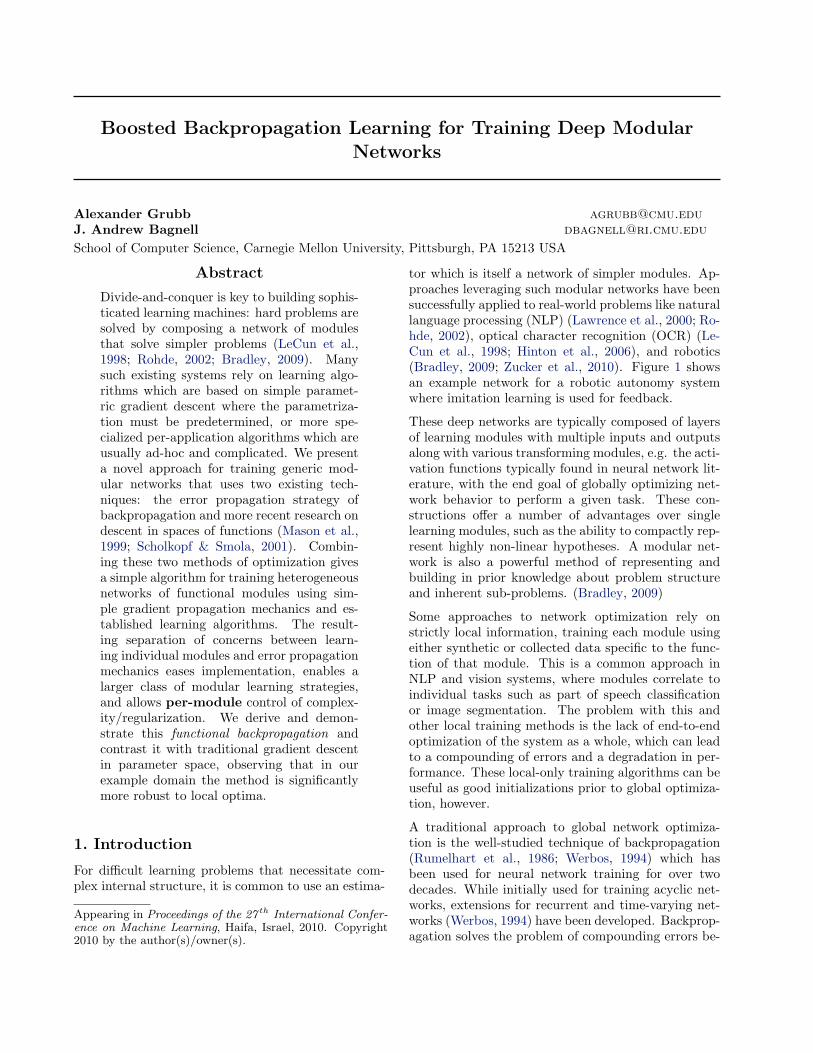
tor which is itself a network of simpler modules. Ap-proaches leveraging such modular networks have beensuccessfully applied to real-world problems like naturallanguage processing (NLP) (Lawrence et al., 2000; Ro-hde, 2002), optical character recognition (OCR) (Le-Cun et al., 1998; Hinton et al., 2006), and robotics(Bradley, 2009; Zucker et al., 2010). Figure 1 showsan example network for a robotic autonomy systemwhere imitation learning is used for feedback.

These deep networks are typically composed of layersof learning modules with multiple inputs and outputsalong with various transforming modules, e.g. the acti-vation functions typically found in neural network lit-erature, with the end goal of globally optimizing net-work behavior to perform a given task. These con-structions offer a number of advantages over singlelearning modules, such as the ability to compactly rep-resent highly non-linear hypotheses. A modular net-work is also a powerful method of representing andbuilding in prior knowledge about problem structureand inherent sub-problems. (Bradley, 2009)

Some approaches to network optimization rely onstrictly local information, training each module usingeither synthetic or collected data specific to the func-tion of that module. This is a common approach inNLP and vision systems, where modules correlate toindividual tasks such as part of speech classificationor image segmentation. The problem with this andother local training methods is the lack of end-to-endoptimization of the system as a whole, which can leadto a compounding of errors and a degradation in per-formance. These local-only training algorithms can beuseful as good initializations prior to global optimiza-tion, however.

A traditional approach to global network optimiza-tion is the well-studied technique of backpropagation(Rumelhart et al., 1986; Werbos, 1994) which hasbeen used for neural network training for over twodecades. While initially used for training acyclic net-works, extensions for recurrent and time-varying net-works (Werbos, 1994) have been developed. Backprop-agation solves the problem of compounding errors be-

Boosted Backpropagation Learning for Modular Networks

tween interacting modules by propagating error infor-mation throughout a network, allowing for end-to-endoptimization with respect to a global measure of error.Further, it can be interpreted as a completely modular(Bottou & Gallinari, 1991), object-oriented approachto semi-automatic differentiation that provides a sep-aration of concerns between modules in the network.

Other approaches for complete optimization of net-works (Hinton et al., 2006; Larochelle et al., 2009) havealso shown promise as alternatives to backpropagation,but many of these algorithms are restricted to specificsystem architectures, and further, often rely upon a”fine-tuning” based on backpropagation. There havehowever been compelling results (Bengio et al., 2007)as to the usefulness of using local module training asan initial optimization step, allowing for rapid learningprior to the traditionally slower global optimizationstep.

The basic backpropagation algorithm has previouslybeen used to provide error signals for gradient descentin parameter space, sometimes making network opti-mization sensitive to the specific parametrization cho-sen. Recently, powerful methods for performing gradi-ent descent directly in a space of functions have beendeveloped both for Reproducing Kernel Hilbert spaces(Scholkopf & Smola, 2001) and for Euclidean functionspaces (Mason et al., 1999; Friedman, 2000).

The former, known as kernel methods, are well studiedin the literature and have been shown to be powerfulmeans for learning non-linear hypotheses. The lattermethods have been shown to be a generalization of theAdaBoost algorithm (Freund & Schapire, 1996), an-other powerful non-linear learning method where com-plex hypotheses are built from arbitrary weak learners.

In the following sections, we present a method forcombining functional gradient descent with backprop-agation. Just as backpropagation allows a separationof concerns between modules, the proposed approachcleanly separates the problem of credit assignment formodules in the network from the problem of learn-ing. This separation allows both a broader class oflearning machines to be applied within the networkarchitecture than standard backpropagation enables,and enables complexity control and generalization per-formance to be managed independently by each mod-ule in the network preventing the usual combinatorialsearch over all modules’ internal complexities simulta-neously. The approach further elucidates the notionof structural local optima—minima that hold in thespace of functions and hence are tied to the modularstructure—as contrasted with parametric local optimawhich are “accidents” of the chosen parameterization.

Figure 1. Modular network from the UPI perception andplanning system for an off-road autonomous vehicle. Imagecourtesy (Bradley, 2009).

We have selected Euclidean functional gradients be-cause of the flexibility provided in choosing base learn-ers and the simplicity of implementing the algorithmin a modular manner. We begin by briefly review-ing Euclidean functional gradient descent, followed bythe modified backpropagation algorithm for functionalgradients. Following that we present a comparison ofparameterized gradient descent and our functional gra-dient based method.

2. Euclidean Functional GradientDescent

In the Euclidean function optimization setting, we seekto minimize a cost functionalR[f ], defined over a set ofsampled points {xn}Nn=1 and accompanying loss func-tions {ln}Nn=1 defined over possible predictions

R[f ] =N∑n=1

ln(f(xn))

by searching over a Euclidean function space F (an L2

space of square-integrable functions) of possible func-tions f .

The desired minimizing function for this cost func-tional can be found using a steepest descent optimiza-tion procedure in function space directly, in contrast toparameterized gradient descent where the gradient isevaluated with respect to the parameters of the func-tion. The functional gradient of R[f ] in this Euclideanfunction space is given as (Gelfand & Fomin, 2000):

∇fR[f ] =N∑i=1

∇f ln(f(xn)) =N∑i=1

l′n(f(xn))δxn

Boosted Backpropagation Learning for Modular Networks

Algorithm 1 Projected Functional Gradient DescentGiven: initial function value f0, step size schedule{αt}Tt=1

for t = 1, . . . , T doCompute gradient ∇fR[f ].Project gradient to hypothesis spaceH using leastsquares projection to find h∗.Update f : ft ← ft−1 − αth∗.

end for

using the chain rule and the fact that ∇ff(xn) = δxn

(Ratliff et al., 2009), where δxnis the Dirac delta func-

tion centered at xn. The resulting gradient is itself afunction composed of the sum of zero-width impulsescentered at the points xn, scaled by the derivative∂+l

∂f(xn) .

Instead of using the explicit functional gradient asthe direction for the gradient step, the gradient isprojected onto a space of functions H, to both al-low for generalization and to constrain the searchspace to some reasonable hypothesis set. The result-ing projected direction h∗ can be found by minimizingthe functional least squares projection of the gradientin L2 function space (Friedman, 2000; Ratliff et al.,2009):

h∗ = argminh∈H

[N∑n=1

(h(xn)−∇fR[f ](xn))2]

(1)

which is equivalent to the familiar least squares regres-sion problem over the dataset {xn,∇fR[f ](xn)}.

These projected gradients are then used to repeatedlyupdate the function, giving the gradient update rulefor f as f(x) ← f(x) − αh∗(x). The final learnedfunction is a sum of gradient steps over time

f(x) = f0(x)−T∑t=1

αtht(x)

where ht(x) is a function representing the gradient steptaken at time t along with the corresponding step sizeαt and starting point f0. A brief description of thisalgorithm is given in Algorithm 1, in a manner thatgeneralizes AdaBoost. (Mason et al., 1999; Friedman,2000)

3. Backpropagation for FunctionalGradients

Using the Lagrangian framework previously developedby LeCun (1988), we now present the first part of ourcontribution: a derivation of backpropagation mechan-ics for functional gradients, both in Euclidean function

space and reproducing kernel Hilbert space (RKHS).In this setting we have a layered network of functionsfk, xnk = fk(xn(k−1)) where n ∈ [1, N ] indexes train-ing examples and k ∈ [1,K] indexes layers. Here xnkrepresents the output of layer k for exemplar n, withxn0 defined to be the training input and xnK the net-work output.

We seek to optimize a subset F ⊆ {fk}Kk=1 of thesefunctions directly while the rest of the functions fk 6∈F remain fixed. These fixed functions are arbitraryactivation or intermediate transformation functions inthe network, and can range from a simple sigmoidfunction to an A* planner.

The optimization of F is with respect to a set of lossfunctions defined over network outputs ln(xnK). Wecan define the local Lagrange function for example nand the complete Lagrange function as

Ln(F,Xn,Λn) = ln(xnK)+K∑k=1

λnkT (xnk − fk(xn(k−1)))

L(F,X,Λ) =N∑n=1

Ln(F,Xn, λn)

with Lagrange multipliers λnk enforcing the forwardpropagation mechanics of the network.

As discussed by LeCun (1988), ∇L(F,X,Λ) = 0 is anecessary condition for any set of functions which area stationary point with respect to the loss functionsln while still satisfying the constraints. This resultsin three separate conditions which must hold at thestationary point:

∂L(F,X,Λ)∂Λ

=∂L(F,X,Λ)

∂X=∂L(F,X,Λ)

∂F= 0 (2)

3.1. Forward Propagation

Satisfying the first condition from (2) yields a separateconstraint for each example n and layer k:

(2) =⇒ ∂L(F,X,Λ)∂λnk

= 0 ∀n, k

=⇒ xnk = fk(xn(k−1)) ∀n, k

These constraints simply re-state the forward propa-gation mechanics of the network.

3.2. Backward Propagation

Similarly, satisfying the second part of (2) providesanother set of constraints over the training data and

Boosted Backpropagation Learning for Modular Networks

layers:

(2) =⇒ ∂L(F,X,Λ)∂xnk

= 0 ∀n, k

=⇒ λnK = l′n(xnK) ∀nλnk = Jfk+1(xnk)λn(k+1) ∀n, k < K

where Jf (X) is the Jacobian matrix of f at X.

These constraints define the mechanics for backwardserror propagation. The Lagrange multipliers λnk storethe accumulated results of applying the chain rule tothe original derivatives of the loss function. Using theordered derivative notation of Werbos (1994), each ele-ment λnki represents the derivative of loss with respectto output xnki, ∂+ln

∂xnki.

3.3. Functional Gradient Update

The final condition in (2) gives a necessary constrainton the final optimized functions in F :

(2) =⇒ ∂L(F,X,Λ)∂fk

= 0 ∀fk ∈ F

=⇒ ∇f [L(F,X,Λ)] = 0 ∀fk ∈ F

=⇒N∑n=1

λnk(∇f [fk(xn(k−1))]) = 0 ∀fk ∈ F

These constraints necessitate that each fk must be afixed point of the Lagrange equation L. Since we seekto minimize the loss functions, a steepest descent pro-cedure can be used to find the minimum with functionupdate rule:

fk ← fk − αN∑n=1

λnk(∇f [fk(xn(k−1))]) ∀fk ∈ F

For RKHS function spaces the functional gradient of afunction itself evaluated at x is the kernel centered atthat point K(x, ·) (Scholkopf & Smola, 2001). Apply-ing this to our functional update we get the followingfunctional update rule:

fk ← fk − αN∑n=1

λnkK(xn(k−1), ·) ∀fk ∈ F

And for Euclidean function spaces (in the idealizedcase) the functional gradient of a function itself isagain the Dirac delta function. Correspondingly, weget the following function update rule:

fk ← fk − αN∑n=1

λnkδxn(k−1) ∀fk ∈ F

Gradient projectionon to H

∇ f F [ f k ]

ht*

nk−1

nk

xn k−1

xnk

Prediction Step Learning Step

xnk=f k xn k−1 f k=∑ t ht*

1

4

2 3

6

5

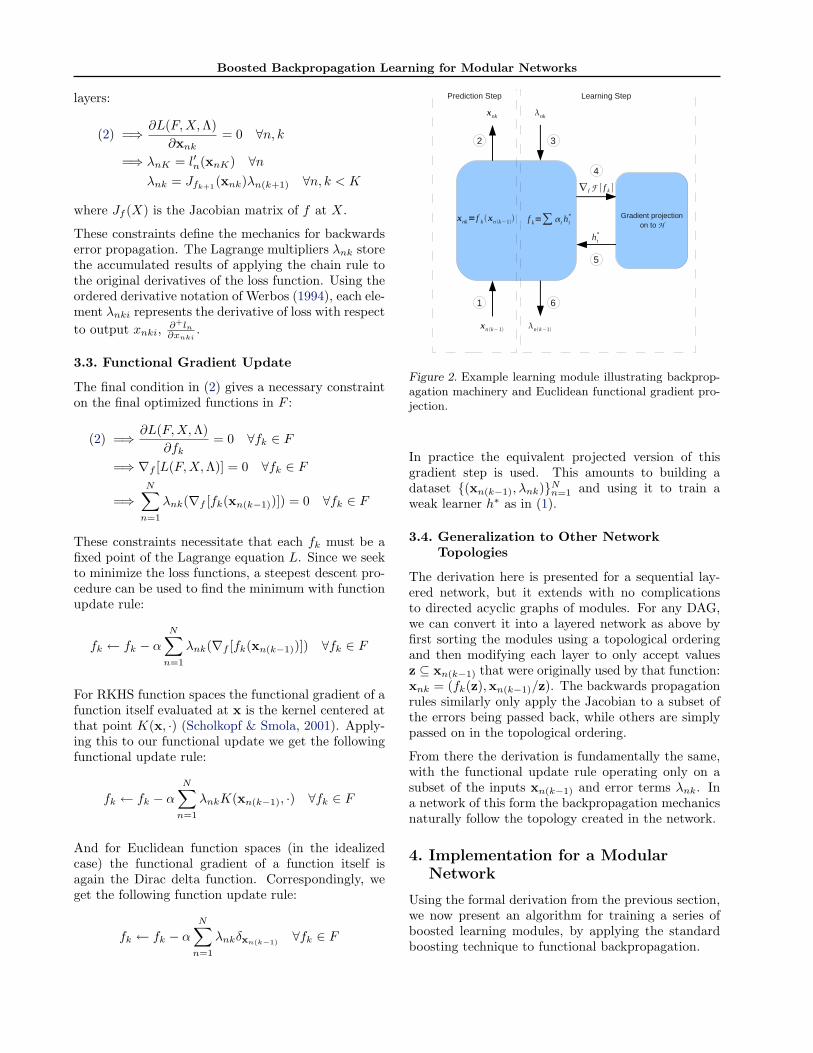
Figure 2. Example learning module illustrating backprop-agation machinery and Euclidean functional gradient pro-jection.

In practice the equivalent projected version of thisgradient step is used. This amounts to building adataset {(xn(k−1), λnk)}Nn=1 and using it to train aweak learner h∗ as in (1).

3.4. Generalization to Other NetworkTopologies

The derivation here is presented for a sequential lay-ered network, but it extends with no complicationsto directed acyclic graphs of modules. For any DAG,we can convert it into a layered network as above byfirst sorting the modules using a topological orderingand then modifying each layer to only accept valuesz ⊆ xn(k−1) that were originally used by that function:xnk = (fk(z),xn(k−1)/z). The backwards propagationrules similarly only apply the Jacobian to a subset ofthe errors being passed back, while others are simplypassed on in the topological ordering.

From there the derivation is fundamentally the same,with the functional update rule operating only on asubset of the inputs xn(k−1) and error terms λnk. Ina network of this form the backpropagation mechanicsnaturally follow the topology created in the network.

4. Implementation for a ModularNetwork

Using the formal derivation from the previous section,we now present an algorithm for training a series ofboosted learning modules, by applying the standardboosting technique to functional backpropagation.

Boosted Backpropagation Learning for Modular Networks

Algorithm 2 Modular Functional Gradient UpdateFunctional Gradient Forward Step:for all xn(k−1) do {Step 1}

Compute outputs xnk = fk(xn(k−1)). {Step 2}end forFunctional Gradient Backward Step:for all λnk do {Step 3}

Compute λn(k−1) = Jfk(xn(k−1))λnk. {Step 6}

end forCompute ∇fL[fk] = λnkδxn(k−1) . {Step 4} 1Project gradient∇fL[fk] on toH using least squaresprojection to find h∗k. {Step 5}Update fk: fkt ← fk(t−1) − αth∗k.

Algorithm 2 gives an outline for computing the forwardand backward propagation steps for each functionallearner in the network. The algorithm for training thecomplete network is the same as in backpropagation: aforward pass through the entire network is computedfor the training data, the gradient of the loss func-tion is evaluated, and then the backward pass prop-agates gradient information through the network andupdates individual modules. Like any gradient-basedprocedure this can be repeated for a fixed number ofsteps or until some measure of convergence is reached.

Unlike standard boosting, there are some restrictionson the weak hypotheses which can be used. To ac-comodate the backpropagation of gradients, the func-tions in the hypothesis space H must be differentiable.Specifically we need to be able to calculate the Jaco-bian Jh for every function h ∈ H. From there theJacobian of each function fk can be easily computedas they are all linear combinations of functions in H.

This restriction does preclude some weak learners com-monly employed in boosting, notably decision stumps,but still allows for a wide range of possible hypothesisspaces. If needed, this restriction can be relaxed forthe first functional learner in a network as no gradientneeds to be propagated through this layer.

A single functional module as described here is pic-tured in Figure 2. Each learning module is composedof machinery for computing the forward step and back-ward gradient propagation step, along with an internalgradient projection module which performs the boost-ing steps necessary to actually update the module.

4.1. Single Output Weak Learners

While the above formalism and algorithm considereach function fk as a multi-output function, in practiceit may be more convenient to treat each function fk asbeing several single-output functions fkj with outputs

xnk = (xnk1, xnk2, . . .), where xnkj = fkj(xn(k−1)).

This is fundamentally equivalent to the multi-outputformulation, but with the restriction that the hypoth-esis space H used for projection is itself a productof a given single-output hypothesis space H = Gmwhere m is the output dimension. The gradient pro-jection step in this restricted hypothesis space is equiv-alent to m independent projections over the datasets{(xn(k−1), λnkj)}Nn=1,∀j.

4.2. Online and Stochastic Learning

The literature on parametric gradient-based learn-ing has shown that stochastic and online versions ofthe standard backpropagation algorithm are highly ef-fective and convenient methods of learning, provid-ing performance improvements and enabling practicallearning from large or even infinite data sources. Bothof these algorithms extend to the functional gradientversions of backpropagation presented here.

For Euclidean functional gradient boosting, while on-line learning on the per-example level is not feasible,an intuitive way of acheiving online behavior is to use“mini-batch” learning where a group of examples iscollected or sampled from the underlying dataset andthis small dataset is used for one iteration of the algo-rithm presented above. Using batches of examples isnecessary in practice to obtain a reasonable and robustfunctional gradient projection.

In the RKHS setting, online learning easily generalizesand is a well studied problem in the literature (Kivinenet al., 2004).

4.3. Benefits of Modularity

This algorithm is inherently modular in two ways: itseparates the individual pieces of the network fromeach other and it separates the structural aspects ofthe network from the learning in individual modules.This feature makes implementing complex networks ofheterogenous modules straightforward and provides anumber of mechanisms for improving learning perfor-mance.

In neural network-based architectures the complexityof the network is usually regulated by changing thestructure of the network in some way. In contrast, thedivision between gradient propagation and gradientprojection when using boosted backpropagation pro-vides a means for varying the complexity of each layerwithout having to alter the structure of the network.

Another key benefit of the separate weak learners isthat the local weak learners can use the gradient beingprojected to validate various local parameters, reduc-

Boosted Backpropagation Learning for Modular Networks

ing the number of parameters and models that needto be globally optimized and validated. For exam-ple, if the weak learner being used is a regularizedleast squares regressor, the regularization parametercan be selected using the gradient dataset and cross-validation. This removes the need for an additionalcombinatorial search for regularization parameters atthe global level, potentially saving a large amount ofcomputation.

5. Experimental Results

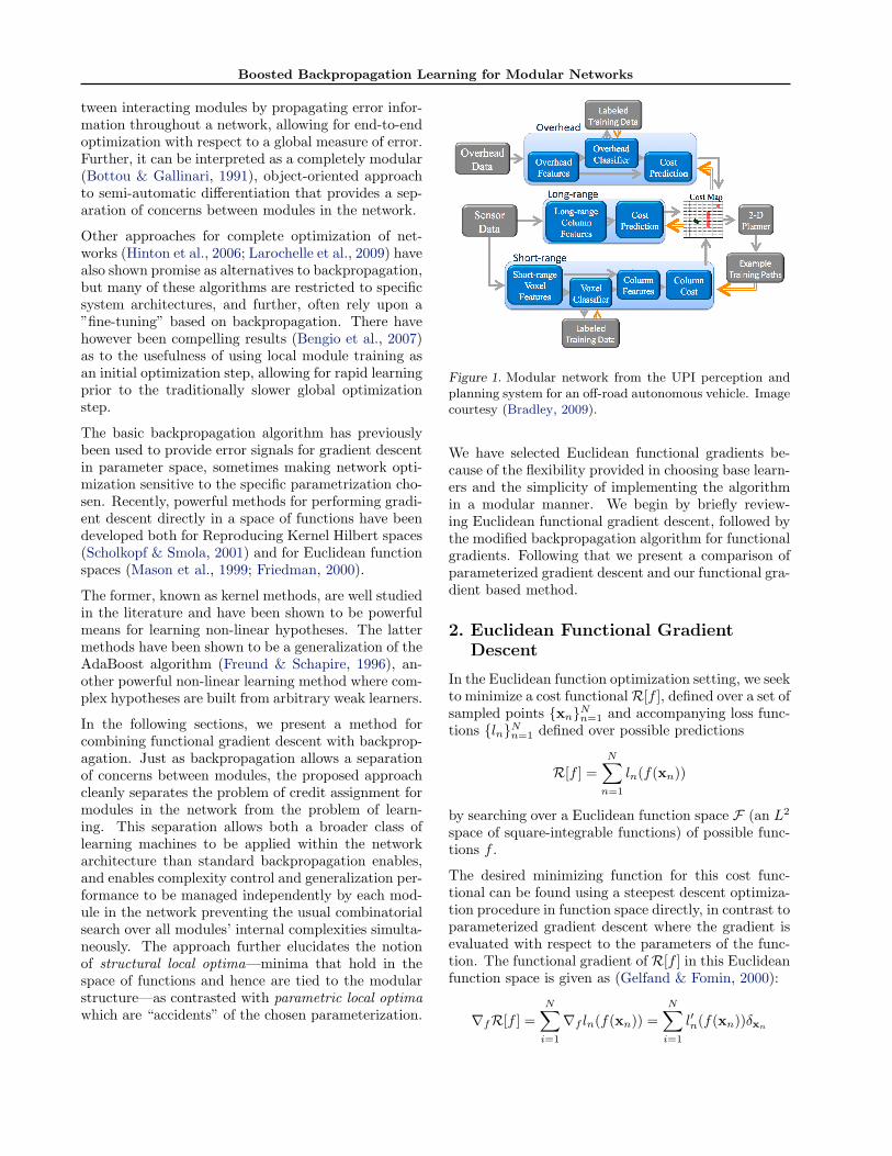
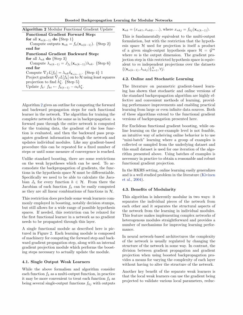
Our experimental application is a simplified path plan-ning system for an autonomous vehicle using Maxi-mum Margin Planning (MMP) (Ratliff et al., 2009),a method for estimating optimal controllers which ex-hibit the same behavior as demonstrated human ex-amples. The planning system, depicted in Figure 3,consists of feature extraction from overhead data, costfunction mapping, and optimal planning (A*, here)modules. We seek to learn both the feature selectionmodule, where raw terrain data is transformed into aset of high-level features, and a cost mapping func-tion which takes the generated high-level features andproduces costs appropriate for planning.

Formally, we are given a set of example mapsM withlocations in these maps x (essentially terrain featureexamples). For the cost function module, we definethe input φ(x) as the output of the feature extractionlayer and then compute output c(φ(x)). The MMPcost functional R is defined as the difference betweenplanned and demonstrated cost

R[c] =1M

M∑i=1

( ∑x∈Mi

c(φ(x))µi(x)−

minµ∈Gi

{ ∑x∈Mi

(c(φ(x))− `i(x))µ(x)})

where µi is the demonstrated path and the minimiza-tion minµ∈Gi

corresponds to the optimal path returnedby the planning algorithm. This cost functional math-ematically expresses the desired constraint that thebehavior of the system after training duplicates thedemonstrated behavior, by ensuring that the lowestcost paths in the examples are in fact the demonstratedpaths. The extra `i(x) term corresponds to a marginfunction designed to ensure the demonstrated behavioris achieved by a significant margin. In our experimentswe use `i(x) = 0 if x is on path µi and 1 otherwise.

The cost functional as given does not appear to fit ourprevious model of a sum of individual loss functions ln,but we can derive the appropriate initial backpropaga-tion gradient by considering the functional gradient of

A* PlannerRaw Terrain DataFeature

ExtractionCost Function

Figure 3. Maximum Margin Planning network for an au-tonomous vehicle. Learning modules are colored in blue,while the planning module is a fixed optimal planner. Inthis case, both a cost function and feature extraction layerare learned simultaneously to improve overall performance.

R directly. This first functional gradient is equivalentto the first λ term from the formal derivation above.

Replacing the minimization with the actual optimalpath according to the planner, µ∗i , we get:

∇fR[c] =1N

N∑i=1

( ∑x∈Mi

µi(x)δφ(x) −∑

x∈Mi

µ∗i (x)δφ(x)

)

∇fR[c] =∑

x∈{SN

i=1Mi}

(1N

(µi(x)(x)− µ∗i(x)(x))δφ(x)

)

Intuitively, this is equivalent to defining a loss functionover outputs yx = c(φ(x)):

lx(yx) = yxµi(x)− (yx − `i)µ∗i (x)where i : x ∈Mi

and using the same machinery formally outlined inSection 3.

Exponentiated Functional Gradient Descent. Anumber of empirical results in the MMP literature(Ratliff et al., 2009) have shown exponentiated func-tional gradient descent to be superior in performance,so we use this method of steepest descent for the cost-ing module. The gradient is calculated in the same wayas before, however instead of using an additive modelas before, we now update the function c(·) using theappropriate exponentiated gradient rule:

c(x) = ec0(x)T∏t=1

eαtht(x)

Similar results can be derived for the parameterizedgradient descent version of this network. In both casesthe initial gradient passed in to the network is identi-cal, and only the learning rule changes.

In the following experiments, the terrain features xare 5 by 5 patches of image data around each location

Boosted Backpropagation Learning for Modular Networks

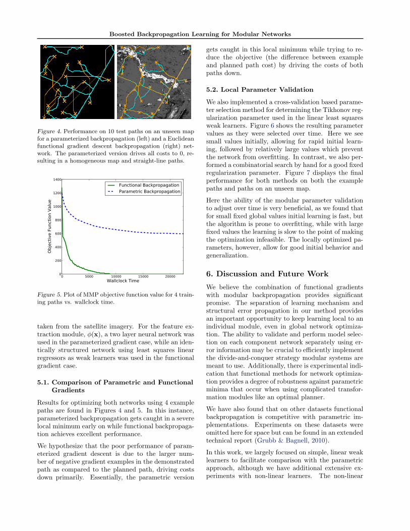
Figure 4. Performance on 10 test paths on an unseen mapfor a parameterized backpropagation (left) and a Euclideanfunctional gradient descent backpropagation (right) net-work. The parameterized version drives all costs to 0, re-sulting in a homogeneous map and straight-line paths.

0 5000 10000 15000 20000Wallclock Time

0

200

400

600

800

1000

1200

1400

Obj

ectiv

e Fu

nctio

n Va

lue

Functional BackpropagationParametric Backpropagation

MMP Objective Function Value vs Time

Figure 5. Plot of MMP objective function value for 4 train-ing paths vs. wallclock time.

taken from the satellite imagery. For the feature ex-traction module, φ(x), a two layer neural network wasused in the parameterized gradient case, while an iden-tically structured network using least squares linearregressors as weak learners was used in the functionalgradient case.

5.1. Comparison of Parametric and FunctionalGradients

Results for optimizing both networks using 4 examplepaths are found in Figures 4 and 5. In this instance,parameterized backpropagation gets caught in a severelocal minimum early on while functional backpropaga-tion achieves excellent performance.

We hypothesize that the poor performance of param-eterized gradient descent is due to the larger num-ber of negative gradient examples in the demonstratedpath as compared to the planned path, driving costsdown primarily. Essentially, the parametric version

gets caught in this local minimum while trying to re-duce the objective (the difference between exampleand planned path cost) by driving the costs of bothpaths down.

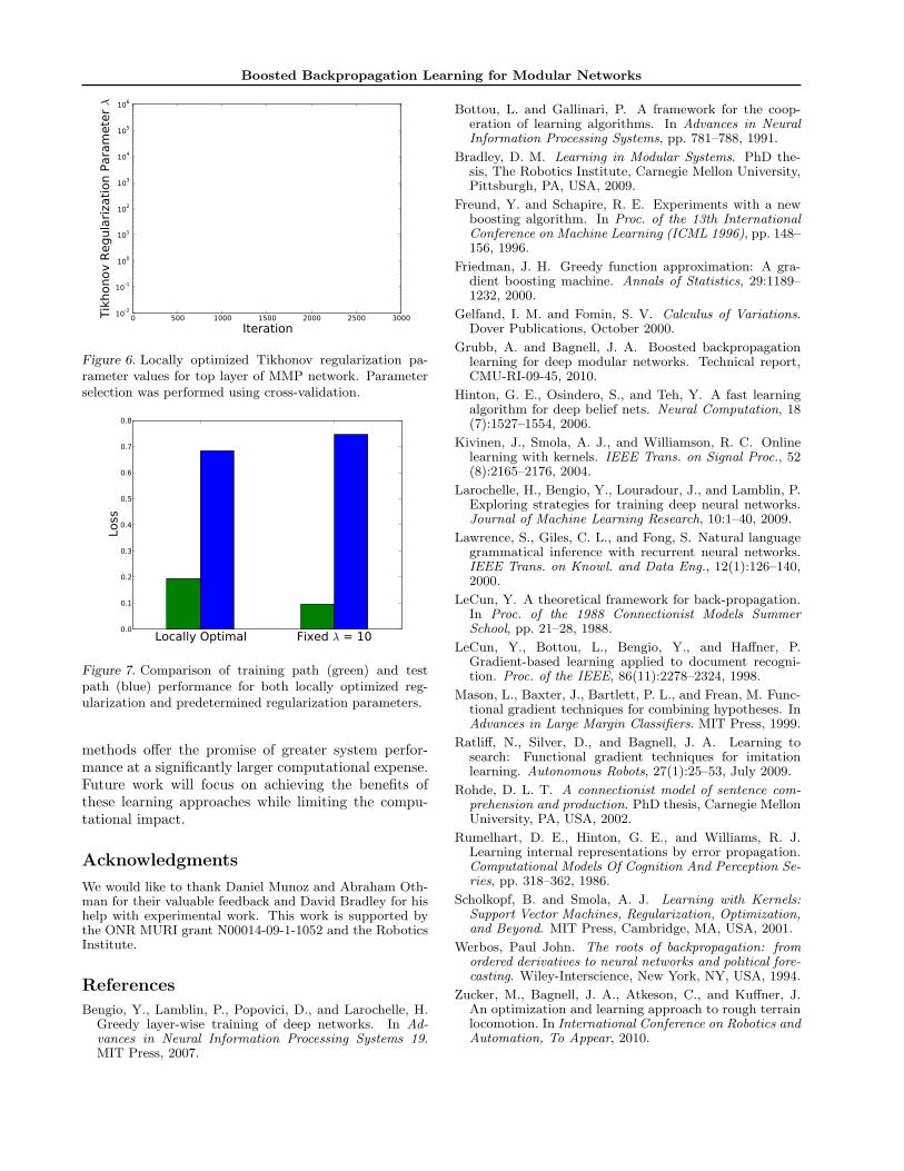
5.2. Local Parameter Validation

We also implemented a cross-validation based parame-ter selection method for determining the Tikhonov reg-ularization parameter used in the linear least squaresweak learners. Figure 6 shows the resulting parametervalues as they were selected over time. Here we seesmall values initially, allowing for rapid initial learn-ing, followed by relatively large values which preventthe network from overfitting. In contrast, we also per-formed a combinatorial search by hand for a good fixedregularization parameter. Figure 7 displays the finalperformance for both methods on both the examplepaths and paths on an unseen map.

Here the ability of the modular parameter validationto adjust over time is very beneficial, as we found thatfor small fixed global values initial learning is fast, butthe algorithm is prone to overfitting, while with largefixed values the learning is slow to the point of makingthe optimization infeasible. The locally optimized pa-rameters, however, allow for good initial behavior andgeneralization.

6. Discussion and Future Work

We believe the combination of functional gradientswith modular backpropagation provides significantpromise. The separation of learning mechanism andstructural error propagation in our method providesan important opportunity to keep learning local to anindividual module, even in global network optimiza-tion. The ability to validate and perform model selec-tion on each component network separately using er-ror information may be crucial to efficiently implementthe divide-and-conquer strategy modular systems aremeant to use. Additionally, there is experimental indi-cation that functional methods for network optimiza-tion provides a degree of robustness against parametricminima that occur when using complicated transfor-mation modules like an optimal planner.

We have also found that on other datasets functionalbackpropagation is competitive with parametric im-plementations. Experiments on these datasets wereomitted here for space but can be found in an extendedtechnical report (Grubb & Bagnell, 2010).

In this work, we largely focused on simple, linear weaklearners to facilitate comparison with the parametricapproach, although we have additional extensive ex-periments with non-linear learners. The non-linear

Boosted Backpropagation Learning for Modular Networks

0 500 1000 1500 2000 2500 3000Iteration

10-2

10-1

100

101

102

103

104

105

106Ti

khon

ov R

egul

ariz

atio

n Pa

ram

eter

λ

Figure 6. Locally optimized Tikhonov regularization pa-rameter values for top layer of MMP network. Parameterselection was performed using cross-validation.

Locally Optimal Fixed λ = 100.0

0.1

0.2

0.3

0.4

0.5

0.6

0.7

0.8

Loss

Figure 7. Comparison of training path (green) and testpath (blue) performance for both locally optimized reg-ularization and predetermined regularization parameters.

methods offer the promise of greater system perfor-mance at a significantly larger computational expense.Future work will focus on achieving the benefits ofthese learning approaches while limiting the compu-tational impact.

Acknowledgments

We would like to thank Daniel Munoz and Abraham Oth-man for their valuable feedback and David Bradley for hishelp with experimental work. This work is supported bythe ONR MURI grant N00014-09-1-1052 and the RoboticsInstitute.

References

Bengio, Y., Lamblin, P., Popovici, D., and Larochelle, H.Greedy layer-wise training of deep networks. In Ad-vances in Neural Information Processing Systems 19.MIT Press, 2007.

Bottou, L. and Gallinari, P. A framework for the coop-eration of learning algorithms. In Advances in NeuralInformation Processing Systems, pp. 781–788, 1991.

Bradley, D. M. Learning in Modular Systems. PhD the-sis, The Robotics Institute, Carnegie Mellon University,Pittsburgh, PA, USA, 2009.

Freund, Y. and Schapire, R. E. Experiments with a newboosting algorithm. In Proc. of the 13th InternationalConference on Machine Learning (ICML 1996), pp. 148–156, 1996.

Friedman, J. H. Greedy function approximation: A gra-dient boosting machine. Annals of Statistics, 29:1189–1232, 2000.

Gelfand, I. M. and Fomin, S. V. Calculus of Variations.Dover Publications, October 2000.

Grubb, A. and Bagnell, J. A. Boosted backpropagationlearning for deep modular networks. Technical report,CMU-RI-09-45, 2010.

Hinton, G. E., Osindero, S., and Teh, Y. A fast learningalgorithm for deep belief nets. Neural Computation, 18(7):1527–1554, 2006.

Kivinen, J., Smola, A. J., and Williamson, R. C. Onlinelearning with kernels. IEEE Trans. on Signal Proc., 52(8):2165–2176, 2004.

Larochelle, H., Bengio, Y., Louradour, J., and Lamblin, P.Exploring strategies for training deep neural networks.Journal of Machine Learning Research, 10:1–40, 2009.

Lawrence, S., Giles, C. L., and Fong, S. Natural languagegrammatical inference with recurrent neural networks.IEEE Trans. on Knowl. and Data Eng., 12(1):126–140,2000.

LeCun, Y. A theoretical framework for back-propagation.In Proc. of the 1988 Connectionist Models SummerSchool, pp. 21–28, 1988.

LeCun, Y., Bottou, L., Bengio, Y., and Haffner, P.Gradient-based learning applied to document recogni-tion. Proc. of the IEEE, 86(11):2278–2324, 1998.

Mason, L., Baxter, J., Bartlett, P. L., and Frean, M. Func-tional gradient techniques for combining hypotheses. InAdvances in Large Margin Classifiers. MIT Press, 1999.

Ratliff, N., Silver, D., and Bagnell, J. A. Learning tosearch: Functional gradient techniques for imitationlearning. Autonomous Robots, 27(1):25–53, July 2009.

Rohde, D. L. T. A connectionist model of sentence com-prehension and production. PhD thesis, Carnegie MellonUniversity, PA, USA, 2002.

Rumelhart, D. E., Hinton, G. E., and Williams, R. J.Learning internal representations by error propagation.Computational Models Of Cognition And Perception Se-ries, pp. 318–362, 1986.

Scholkopf, B. and Smola, A. J. Learning with Kernels:Support Vector Machines, Regularization, Optimization,and Beyond. MIT Press, Cambridge, MA, USA, 2001.

Werbos, Paul John. The roots of backpropagation: fromordered derivatives to neural networks and political fore-casting. Wiley-Interscience, New York, NY, USA, 1994.

Zucker, M., Bagnell, J. A., Atkeson, C., and Kuffner, J.An optimization and learning approach to rough terrainlocomotion. In International Conference on Robotics andAutomation, To Appear, 2010.