Bonds, Bond Prices, Interest Rates, and the Riskand Term Structure of Interest Rates

ECON 40364: Monetary Theory & Policy

Eric Sims

University of Notre Dame

Fall 2017

1 / 68

Readings

I Text:I Mishkin Ch. 4, Mishkin Ch. 5 pg. 85-100, Mishkin Ch. 6

I Other:I Poole (2005): “Understanding the Term Structure of Interest

Rates”I Bernanke (2016), “What Tools Does the Fed Have Left? Part

2: Targeting Longer-Term Interest Rates”

2 / 68

Bonds

I We will generically refer to a “bond” as a debt instrumentwhere a borrower promises to pay the holder of the bond (thelender) interest plus principal at some known date

I There are many different types of bonds. Differ according to:I Details of how bond is paid offI Time to maturityI Default risk

I The yield to maturity is a measure of the interest rate on thebond, although the interest rate is often not explicitly laidout. Will use terms interest rate and yield interchangeably

I Want to understand how interest rates are determined andhow and why they vary across different characteristics ofbonds

3 / 68

Present ValueI Present discounted value (PDV): a dollar in the future is

worth less than a dollar in the presentI You “discount” future payouts relative to the present because

you could put money “in the bank” in the present and earninterest

I For a future cash flow (CF ), how many dollars would beequivalent to you today:

PVt =CFt+n

(1 + it)(1 + it+1)(1 + it+2) · · · × (1 + it+n−1)

I Here t is the “present,” t + n is the future (n periods away),and it , it+1, . . . are the one period interest rates betweenperiods

I If it = it+1 = · · · = it+n−1 = i , then formula reduces to:

PVt =CFt+n

(1 + i)n

4 / 68

Present Value: Example I

I Suppose you are promised $10 in period t + 1

I You could put $1 in bank in period t and earn it = 0.05 ininterest between t and t + 1

I How many dollars would you need in the present to have $10in the future?

(1 + it)PVt = CFt+1

PVt =CFt+1

1 + it

=10

1.05= 9.5238

5 / 68

Present Value: Example II

I Suppose you are promised $10 in period t + 3

I You could put $1 in bank in period t and earn it = 0.05 ininterest between t and t + 1

I You expect to be able to earn interest of it+1 = 0.07 betweent + 1 and t + 2 and it+2 = 0.03 between t + 2 and t + 3

I If you put $1 in bank in period t and kept it there(re-investing any interest income), you would have(1 + it)(1 + it+1)(1 + it+2) dollars in t + 3. Hence, thepresent value of $10 three periods from now is:

PVt(1 + it)(1 + it+1)(1 + it+2) = CFt+3

PVt =CFt+3

(1 + it)(1 + it+1)(1 + it+2)

=10

(1.05)(1.07)(1.03)= 8.6415

6 / 68

Present Value and the Price of an Asset

I A financial asset is something which entitles the holder toperiodic payments (cash flows)

I The classical theory of asset prices is that the price of an assetis equal to the present discounted value of all future cash flows

I A bond is an asset: it entitles you to periodic cash flows. Astock is another kind of financial asset

I Price is just the present discounted value of cash flows

I The yield or interest rate on an asset is the interest rate youuse to discount those future cash flows

7 / 68

Different Types of Bonds

I The following are different types of bonds/debt instrumentsdepending on the nature of how they are paid back:

1. Simple loan: you borrow X dollars and agree to pay back(1 + i)X dollars at some specified date (interest plus principal)(e.g. commercial loan)

2. Fixed payment loan: you borrow X dollars and agree to payback the same amount each period (e.g. month) for a specifiedperiod of time. “Full amortization” (e.g. fixed rate mortgage)

3. Coupon bond: you borrow X dollars and agree to pay backfixed coupon payments, C , each period (e.g. year) for aspecified period of time (e.g. 10 years), at which time you payoff the “face value” of the bond (e.g. Treasury Bond)

4. Discount bond: you borrow X dollars and agree to pay back Ydollars after a specified period of time with no payments in theintervening periods. Typically, Y > X , so the bond sells “at adiscount” (e.g. Treasury Bill)

I Interest rate is not explicit for coupon or discount bonds

8 / 68

Yield to Maturity

I The yield to maturity (YTM) is the (fixed) interest rate thatequates the PDV of cash flows with the price of the bond inthe present

I This measures the return (expressed at an annualized rate)that would be earned on holding a bond if it is held untilmaturity

I The YTM does not necessarily correspond to the return if thebond is not held until maturity (i.e. if you sell a bond beforeits maturity date)

I The YTM is another way of conveying the price of a bond,taking future cash flows as given

9 / 68

YTM on a Simple Loan

I The YTM on a simple loan is just the contractual interest rate

I For a one period loan, the YTM is the same thing as thereturn

I Let P be the price of the loan, CF the payout after one year,and i the interest rate. Then:

P =CF

1 + i

I Or:

1 + i =CF

P

I Or:

i =CF − P

P

I Where CF−PP is the return (or rate of return) on the loan

10 / 68

Price and Yield on a Simple Loan

800 820 840 860 880 900 920 940 960 980 1000P

0

0.05

0.1

0.15

0.2

0.25Y

TM

1 Year Maturity, F = 1000, Simple Loan

11 / 68

YTM on a Discount Bond

I The YTM on a discount bond is similar to a simple loan, justwith different maturities

I In particular, for a face value of F , maturity of n, and price ofP, the YTM satisfies:

P =F

(1 + i)n

I Or:

1 + i =

(F

P

) 1n

12 / 68

Price and Yield on a Discount Bond

500 550 600 650 700 750 800 850 900 950 1000P

0

0.01

0.02

0.03

0.04

0.05

0.06

0.07

0.08Y

TM

10 Year Maturity, F = 1000, Discount Bond

13 / 68

YTM on a Coupon Bond

I Suppose a bond has a face value of $100 and a maturity ofthree years

I It pays coupon payments of $10 in years t + 1, t + 2, andt + 3 (the coupon rate in this example is 10 percent)

I The face value is paid off after period t + 3

I The period t price of the bond is $100

I The YTM solves:

100 =10

1 + i+

10

(1 + i)2+

10

(1 + i)3+

100

(1 + i)3

I Which works out to i = 0.1

I More generally, for an n period maturity:

P =n

∑j=1

C

(1 + i)j+

FV

(1 + i)n

14 / 68

Price and Yield on a Coupon Bond

800 850 900 950 1000 1050 1100 1150 1200P

0.08

0.085

0.09

0.095

0.1

0.105

0.11

0.115

0.12

0.125

0.13Y

TM

30 Year Maturity, F = 1000, Coupon Rate = 10 Percent

15 / 68

Perpetuities

I Perpetuities (also called “consols”) are like coupon bonds,except they have no maturity date

I Here, the relationship between price, yield, and couponpayments works out cleanly and is given by:

i =C

P

I For a coupon bond with a sufficiently long maturity, this is areasonable approximation to the bond’s YTM (because thePDV of the face value after many years is close to zero)

I This expression is also sometimes called the current yield asan approximation to the YTM on a coupon bond

16 / 68

Price and Yield on a Perpetuity

1000 1100 1200 1300 1400 1500 1600 1700 1800 1900 2000P

0.05

0.055

0.06

0.065

0.07

0.075

0.08

0.085

0.09

0.095

0.1Y

TM

Perpetuity, C = 100

17 / 68

Observations

I Several observations are noteworthy from the previous slides:

1. The bond price and yield are negatively related. This is truefor all types of bonds. Bond prices and interest rates move inopposite directions

2. For discount bonds, we would not expect price to be greaterthan face value – this would imply a negative yield

3. For a coupon bond, when the bond is priced at face value, theyield to maturity equals the coupon rate

4. For a coupon bond, when the bond is priced less than facevalue, the YTM is greater than the coupon rate (andvice-versa)

18 / 68

Yields (Interest Rates) and ReturnsI Returns and yields (interest rates) are in general not the same

thingI Rate of return: cash flow plus new security price, divided by

current priceI Useful way to think about it (terminology here is related to

equities): “dividend rate plus capital gain,” where capital gainis the change in the security’s price

I The return on a coupon bond held from t to t + 1 is:

R =C + Pt+1 − Pt

Pt

I Or:

R =C

Pt︸︷︷︸Current Yield

+Pt+1 − Pt

Pt︸ ︷︷ ︸Capital Gain

I Return will differ from current yield (approximation to YTM)if bond prices fluctuates in unexpected ways

19 / 68

Discount Bond

I Suppose that you hold a discount bond with face value $1000,a maturity of 30 years, and a current yield to maturity of 10percent

I The current price of this bond is 10001.130

= 57.31.

I Suppose that interest rates stay the same after a year. Thenthe bond has a price of 1000

1.129= 63.04

I Since there is no coupon payment, your one year holdingperiod return (holding period refers to length of time you holdthe security) is just the capital gain:

R =Pt+1 − Pt

Pt=

63.04− 57.31

57.31= 0.10

I If interest rates do not change, then the return and the yieldto maturity are the same thing

20 / 68

Interest Rate Risk

I Continue with the same setup

I But now suppose that interest rates go up to 15 percent inperiod t + 1 and are expected to remain there

I Then the price of the bond in period t + 1 will be:10001.1529

= 17.37

I Your return is then:

R =Pt+1 − Pt

Pt=

17.37− 57.31

57.31= −0.69

I On a discount bond, an increase in interest rates exposes youto large capital loss

21 / 68

Return and Time to Maturity, Coupon Bond

0 5 10 15 20 25 30Time to Maturity

-0.25

-0.2

-0.15

-0.1

-0.05

0

0.05

0.1R

Interest Rate Increase from 10 to 15 Percent, 10 Percent Coupon Rate, F = 1000

22 / 68

ObservationsI Return and initial YTM are equal if the holding period is the

same as time to maturity (1 period). The capital gain issimply the face value (which is fixed) minus the initial price

I Increase in interest rates results in returns being less thaninitial yield

I Reverse is trueI Return is more affected by interest rate change the longer is

the time to maturityI If you hold the bond until maturity, your return is locked in at

initial YTMI Concept of return is relevant even if you do not sell the bond

and realize the capital loss. There is an opportunity cost – ifinterest rates rise, had you not locked yourself in on a longmaturity bond you could have purchased a bond in the futurewith a higher yield

I Longer maturity bonds are therefore riskier than shortmaturity bonds

23 / 68

Determinants of Bond Prices (and interest rates)

I What determines bond prices and interest rates?

I Supply and demand!

I Though there are many different kinds of bonds and manydifferent kinds of issuers of bonds, think about a world inwhich there is just one type of bond (and just one type ofinterest rate)

I For simplicity, think of this as a discount bound

I Remember: bond prices and interest rates move opposite oneanother

24 / 68

Portfolio Choice

I Our theory of demand of a bond (or any asset) is thatdemand is based on the following factors:

1. Wealth: assets are normal goods, so the more wealth, themore you want to hold at every price

2. Expected returns: you hold assets to earn returns. The higherthe expected return, the more of it you demand

3. Risk: assume agents are risk averse. Holding expected returnconstant, you would prefer a less risky return. The more riskyan asset is, the less of it you demand

4. Liquidity: refers to the ease with which you can sell an asset.The more liquid it is, the more attractive it is to hold (it’seasier to sell if you need to raise cash in a pinch)

25 / 68

Demand for Bonds

I How does the demand for bonds vary with the price of bonds?

I As the price goes down, the interest rate goes up

I Therefore, holding everything else fixed, the expected returnon holding a bond goes up as the price falls

I Therefore, demand slopes down

I Demand will shift (change in quantity demanded for a givenprice) with changes in other factors

26 / 68

Bond Demand

𝑃

𝑄

𝐷

Shifts right if: (i) Wealth goes up (ii) Expected return goes up (iii) Riskiness goes down (iv) Liquidity goes up

27 / 68

Supply of Bonds

I Issuers of bonds are borrowers. You are issuing a bond to raisefunds in the present to be paid back in the future

I Recall that bond prices move opposite interest rates

I As the bond price increases, the yield decreases

I Therefore, at a higher bond price, the cost of borrowing islower

I So there will be more supply of bonds at a higher price –supply slopes up

I Changes in other factors, holding price fixed, will cause thesupply curve to shift

28 / 68

Bond Supply

𝑃

𝑄

𝑆

Shifts right if: (i) Expected profitability

goes up (ii) Expected inflation

goes up (iii) Government deficit

goes up

29 / 68

Bond Market Equilibrium

𝑃𝑃

𝑄𝑄

𝑆𝑆

𝐷𝐷

𝑃𝑃∗

𝑄𝑄∗

30 / 68

Equilibrium

I The intersection of supply and demand determines theequilibrium price and quantity of bonds

I By determining price, the equilibrium effectively determinesthe interest rate, which is inversely related to price

I An alternative way to think about equilibrium is the marketfor loanable funds

I The loanable funds diagram puts the interest rate (rather thanbond price) on the vertical axis, and essentially swaps whodemands and who supplies:

I In the previous setup, savers demand bonds whereas borrowerssupply bonds

I In the loanable funds setup, savers supply funds whereasborrowers demand funds

I We call the supply curve the supply of savings, and thedemand curve the demand for investment. In equilibrium, wemust have S = I

31 / 68

Loanable Funds Diagram

𝑖𝑖

𝑆𝑆, 𝐼𝐼

𝑆𝑆

𝐼𝐼

𝑖𝑖∗

𝑆𝑆∗ = 𝐼𝐼∗

32 / 68

An Increase in Risk

𝑃𝑃

𝑄𝑄

𝑆𝑆

𝐷𝐷

𝑄𝑄0∗

𝐷𝐷′

𝑄𝑄1∗

𝑃𝑃0∗

𝑃𝑃1∗

An increase in perceived risk reduces demand for bonds, resulting in lower bond prices and higher interest rates

33 / 68

An Increase in Liquidity

𝑃𝑃

𝑄𝑄

𝑆𝑆

𝐷𝐷

𝑄𝑄0∗

𝐷𝐷′

𝑄𝑄1∗

𝑃𝑃0∗

𝑃𝑃1∗ An increase in liquidity increases demand, raises bond prices, and therefore lowers interest rates

34 / 68

An Increase in Expected Future Interest Rates

𝑃𝑃

𝑄𝑄

𝑆𝑆

𝐷𝐷

𝑄𝑄0∗

𝐷𝐷′

𝑄𝑄1∗

𝑃𝑃0∗

𝑃𝑃1∗

An increase in expected future interest rates lowers expected bond returns. This shifts the demand curve in, resulting in a lower price and higher yield

35 / 68

An Increase in Government Budget Deficit

𝑃𝑃

𝑄𝑄

𝑆𝑆

𝐷𝐷

𝑄𝑄0∗ 𝑄𝑄1∗

𝑃𝑃0∗

𝑃𝑃1∗

An increase in government budget deficits causes the supply of bonds to shift to the right, resulting in lower bond prices and higher interest rates

𝑆𝑆′

36 / 68

Different Bond Characteristics

I Bonds with the same cash flow details (e.g. discount bondsvs. coupon bonds vs. perpetuities) nevertheless often havevery different yields

I Why is this?I Aside from details about cash flows, bonds differ principally

on two dimensions:

1. Default risk2. Time to maturity

37 / 68

Default Risk

I Default occurs when the borrower decides to not make goodon a promise to pay back all or some of his/her outstandingdebts

I We think of federal government bonds as being (essentially)default-free: since government can always “print” money,should not explicitly default (though monetization of debt iseffectively form of default)

I Corporate (and state and local government) bonds do havesome default risk

I Rating agencies: Aaa is highest rated, then Bs, then Csmeasure credit risk of lenders

I Risk premium: difference (i.e. spread) between yield onrelatively more risky debt (e.g. Aaa corporate debt) and lessrisk debt (e.g. government debt), assuming same time tomaturity

38 / 68

Yields on Different Bonds

39 / 68

Observations

I We see more or less exactly the pattern we would expect fromour demand/supply analysis – risker bonds have higher yields

I Obvious exception: municipal bonds

I Why? Interest income on these bonds is exempt from federaltaxes, which makes their expected returns higher, andtherefore drives up price (and drives down yield)

I Important: interesting time variation in spreads (see nextcouple of slides)

40 / 68

myf.red/g/dU3z

-0.5

0.0

0.5

1.0

1.5

2.0

2.5

3.0

3.5

1984 1986 1988 1990 1992 1994 1996 1998 2000 2002 2004 2006 2008 2010 2012 2014 2016

fred.stlouisfed.orgSource:FederalReserveBankofSt.Louis

Moody'sSeasonedAaaCorporateBondYieldRelativetoYieldon10-YearTreasuryConstantMaturity©

Percent

41 / 68

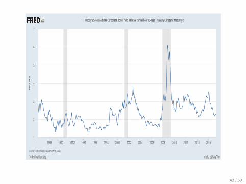
myf.red/g/dTre

1

2

3

4

5

6

7

1988 1990 1992 1994 1996 1998 2000 2002 2004 2006 2008 2010 2012 2014 2016

fred.stlouisfed.orgSource:FederalReserveBankofSt.Louis

Moody'sSeasonedBaaCorporateBondYieldRelativetoYieldon10-YearTreasuryConstantMaturity©

Percent

42 / 68

Countercyclical Default Risk

I It stands to reason that default risk ought to be high wheneconomy is in recession

I When default risk is high, we might expect a “flight tosafety”: reduces demand for risky bonds and increasesdemand for riskless bonds, which moves credit spread up

I This is consistent with what we see in the previous slides:credit spreads tend to rise during recessions

43 / 68

Flight to Safety

𝑃𝑃 𝑃𝑃 𝑆𝑆 𝑆𝑆

𝐷𝐷 𝐷𝐷

𝑄𝑄 𝑄𝑄

𝑃𝑃0 𝑃𝑃0

𝑄𝑄0 𝑄𝑄0

𝐷𝐷′

𝐷𝐷′

Corporate Bonds Government Bonds

𝑃𝑃1

𝑃𝑃1

𝑄𝑄1 𝑄𝑄1

44 / 68

Yields During Great Recession

2.003.004.005.006.007.008.009.00

10.00

Yields and the Great Recession

Baa Aaa 10 Yr Treasury

45 / 68

Term Structure of Interest Rates

I Bonds with otherwise identical cash flows and riskcharacteristics can have different times to maturity (or justmaturities, for short)

I How do yields vary with time to maturity for a bond withotherwise identical characteristics?

I A plot of yields on bonds against the time to maturity isknown as a yield curve

46 / 68

47 / 68

0

1

2

3

4

5

6

1 mo 3 mo 6 mo 1 yr 2 yr 3 yr 5 yr 7 yr 10 yr 20 yr 30 yr

Yie

ld t

o M

atu

rity

Time to Maturity

2017

2014

2011

2009

2008

2007

48 / 68

Observations

I The following observations can be made from previous twopictures

1. Yields on bonds of different maturities tend to move together2. Yield curves are upward-sloping most of the time

I The slope of the yield curve is often predictive of recession.Flat or downward-sloping (“inverted”) yield curves oftenprecede recessions

3. When short term interest rates are low, yield curves are morelikely to be upward-sloping

49 / 68

Yield Curves Prior to Recent Recessions

0

1

2

3

4

5

6

7

8

9

3 mo 6 mo 1 yr 2 yr 3 yr 5 yr 7 yr 10 yr 30yr

Yie

ld t

o M

atu

rity

Time to Maturity

2007

2000

1990

50 / 68

Theories of the Yield Curve

I We would like to understand the term structure of interestrates:

1. Expectations hypothesis2. Segmented markets3. Liquidity premium theory

I The liquidity premium theory essentially combines (1) and (2)

51 / 68

Expectations HypothesisI Expectations hypothesis: the yield on a long maturity bond is the

average of the expected yields on shorter maturity bonds

I For example, suppose you consider 1 and 2 year bonds

I The yield on a 1 year bond is 4 percent; you expect the yield on a 1year bond one year from now to be 6 percent

I Then the yield on a two year bond ought to be 5 percent(0.5× (4 + 6) = 5)

I Why? If you buy a two 1 year bonds in succession, your yield overthe two year period is (approximately, ignoring compounding) 10percent – (1 + 0.04)× (1 + 0.06)− 1 = 0.1024 ≈ 0.10

I If the 2 and 1 year bonds are perfect substitutes, the yield on thetwo year bond has to be the same: (1 + i)2 = 0.1⇒ i ≈ 0.05

I Demand and supply: if you expect future short yields to rise, this

lowers expected profitability of long term bonds in the present,

reducing demand, driving down price, and driving up yield: current

long term yield tells you something about expected future short

term yields

52 / 68

Simple Theory Behind the Expectations Hypothesis

I A household lives for three periods: t, t + 1, and t + 2.Consumes (C ) and earns income (Y ). Lifetime utility:

U = lnCt + β lnCt+1 + β2 lnCt+2

I In period t, can save in either a one period bond, B1,t , or atwo period bond, B2,t . Normalize prices in t to 1, with yields(interest rates) of i1,t and i2,t (could equivalently make thesediscount bonds with future prices of 1 and current prices lessthan 1 with yields implicit rather than explicit)

I In period t + 1, can save in a one period discount bond,B1,t+1, with yield of i1,t+1. Sequence of budget constraints:

Ct + B1,t + B2,t = Yt

Ct+1 + B1,t+1 = Yt+1 + (1 + i1,t)B1,t

Ct+2 = Yt+2 + (1 + i1,t+1)B1,t+1 + (1 + i2,t)2B2,t

53 / 68

Optimality ConditionsI The optimality conditions can be written as a sequence of

Euler equations:

1

Ct= β

1

Ct+1(1 + i1,t)

1

Ct+1= β

1

Ct+2(1 + i1,t+1)

1

Ct= β2 1

Ct+2(1 + i2,t)

2

I If you combine these, you get:

(1 + i1,t)(1 + i1,t+1) = (1 + i2,t)2

I Which is approximately:

i2,t ≈1

2[i1,t + i1,t+1]

54 / 68

More Generally

I For a bond with a maturity of n periods, the expectationstheory tells us:

in,t =it + iet+1 + · · ·+ iet+n−1

n

I Yields after period t have e superscripts to denote that theyare expectations

I Observing in,t and it in period t, this relationship can be usedto infer market expectations of future short term interest rates(“forward rates”). In particular:

iet+1 = 2i2,t − it

iet+2 = 3i3,t − 2i2,t...

iet+h = (h+ 1)ih+1,t − hih,t

55 / 68

Implied 1 Year Ahead Forward Rate

0

1

2

3

4

5

6

7

8

9

10

1991 1994 1997 2000 2003 2006 2009 2012 2015

Forward Rate 1 Yr Ago

Realized 1 Yr Rate

56 / 68

Implied 2 Year Ahead Forward Rate

0

1

2

3

4

5

6

7

8

9

10

1992 1995 1998 2001 2004 2007 2010 2013 2016

Forward Rate 2 Yrs Ago

Realized 1 Yr Rate

57 / 68

Evaluating the Expectations Hypothesis

I Expectations hypothesis can help make sense of several facts:

1. Long and short term rates tend to move together. If currentshort term rates are low and people expect them to stay lowfor a while (interest rates are quite persistent), then long termyields will also be low

2. Why a flattening/inversion of yield curve can predictrecessions. If people expect economy to go into recession, theywill expect the Fed to lower short term interest rates in thefuture. If short term interest rates are expected to fall, thenlong term rates will fall relative to current short term rates,and the yield curve will flatten.

I Where the expectations hypothesis fails: why are yield curvesalmost always upward-sloping? If interest rates aremean-reverting, then the average yield curve ought to be flat,not upward-sloping

58 / 68

Segmented Markets Hypothesis

I The Expectations Hypothesis assumes that bonds of differentmaturities are perfect substitutes, which forces expectedreturns to be equal across bonds of differing maturities

I Segmented Markets is the polar extreme: bonds of differentmaturities aren’t substitutes at all

I If this is the case, there is no reason for returns to be equalized

I Furthermore, since longer maturity bonds are subject to moreinterest rate risk, there will in general be more demand forshort term bonds than long term bonds

I This means that the price of short term bonds will be highrelative to long term bonds, meaning that long term bondswill have higher yields

I Hence, segmented markets can explain why yield curves slopeup most of the time

59 / 68

Liquidity Premium Theory

I Segmented markets hypothesis cannot explain why interestrates of different maturities tend to move together, or accountfor why you can predict future short term rates from longterm yields

I Liquidity premium theory: essentially combines expectationshypothesis with market segmentation

I Bonds of different maturities are substitutes, but not perfectsubstitutes: savers demand higher yields on longer term bondsbecause of their heightened risk

I Relationship between long and short rates:

in,t =it + iet+1 + . . . iet+n−1

n︸ ︷︷ ︸Expectations Hypothesis

+ ln,t︸︷︷︸Liquidity Premium

I The liquidity premium, ln,t , is increasing in the time tomaturity

60 / 68

61 / 68

A First Look at Quantitative Easing and UnconventionalMonetary Policy

I The interest rates relevant for most investment andconsumption decisions are long term (e.g. mortgage) andrisky (e.g. Baa corporate bond)

I Conventional monetary policy targets short term and risklessinterest rates (e.g. Fed Funds Rate)

I Out theory of of bond pricing helps us understand theconnection between the these different kinds of interest rates

62 / 68

Monetary Policy in Normal Times

I Think of a world where the liquidity premium theory holds(with a fixed liquidity premium)

I A central bank lowers (raises) short term interest rates and isexpected to keep these low (high) for some time

I This ought to also lower (raise) longer term rates to theextent to which longer term rates are the average of expectedshorter term rates

I Holding risk factors constant, substitutability between bondsmeans that riskier yields also ought to fall (increase)

I Simulation:I Consider 1 period, 10 year, 20 year, and 30 year bondsI Fixed liquidity premia of 1, 2, and 3I Short term rate is cut from 4 to 3 persistentlyI Simulate yields for 30 quarters (one-fourth of a year)

63 / 68

Theoretical Simulation

0 10 20 30Quarters

3

4

5

6

7

8

Yield

s

No Cut

Short Rate10 Year20 Year30 Year

0 10 20 30Quarters

3

4

5

6

7

8

Yield

s

Rate Cut

64 / 68

Monetary Loosening and Tightening in Historical Episodes

5.0000

6.0000

7.0000

8.0000

9.0000

10.0000

11.0000

FFR

AAA

Baa

Mortgage

10 Yr Treasury2.0000

3.0000

4.0000

5.0000

6.0000

7.0000

8.0000

9.0000

10.0000

FFR

Aaa

Baa

Mortgage

10 Yr Treasury

65 / 68

Monetary Loosening and Tightening in Historical Episodes

0.00001.00002.00003.00004.00005.00006.00007.00008.00009.0000

20

00

-1

2-0

1

20

01

-0

1-0

1

20

01

-0

2-0

12

00

1-0

3-0

1

20

01

-0

4-0

12

00

1-0

5-0

1

20

01

-0

6-0

12

00

1-0

7-0

1

20

01

-0

8-0

1

20

01

-0

9-0

12

00

1-1

0-0

1

20

01

-1

1-0

12

00

1-1

2-0

1

20

02

-0

1-0

1

20

02

-0

2-0

1

FFR

Aaa

Baa

Mortgage

10 Yr Treasury0.0000

1.0000

2.0000

3.0000

4.0000

5.0000

6.0000

7.0000

8.0000

FFR

Aaa

Baa

Mortgage

10 Yr Treasury

66 / 68

Term Structure Puzzle?

I If you look at last two pictures, in the 1990s other ratestracked the FFR reasonably closely, but this falls apart in the2000s

I This has been referred to as the term structure puzzle and isdiscussed in Poole (2005)

I From perspective of expectations hypothesis, would expectlonger maturity, riskier rates to move along with shortermaturity rates. Not what we see in 2000s

I But two key issues:I Forecastability: if people expected the Fed to raise rates

starting in 2004/2005 from the perspective of 2002/2003, thiswould have been incorporated into long rates before the FFRstarted to move. Most people think Fed policy has becomemore forecastable

I Persistence: behavior of long rates depends on how persistentchanges in short rates are expected to

67 / 68

Unconventional Monetary Policy

I In a world where Fed Funds Rate is at or very near zero,conventional monetary loosening isn’t on the table

I Unconventional monetary policy:

1. Quantitative Easing (or Large Scale Asset Purchases):purchases of longer maturity government debt or risky privatesector debt. Idea: raise demand for this debt, raise price, andlower yield. See here

2. Forward Guidance: promises to keep future short term interestrates low. Idea is to work through expectations hypothesis andto lower long term yields immediately. See here

I Ben Bernanke: “The problem with quantitative easing is thatit works in practice but not in theory”

I Under expectations hypothesis, cannot affect long term yieldswithout impacting path of short term yields

I Must either impact liquidity premium or be a form of forwardguidance

68 / 68