Bond Graph Based Sensitivity and Uncertainty Analysis Modelling...
15
Bond Graph Based Sensitivity and Uncertainty Analysis Modelling for Micro-Scale Multiphysics Robust Engineering Design M. A. Perry, a,* M. A. Atherton, b R. A. Bates, a H. P. Wynn. a a Dept. of Statistics, London School of Economics, London WC2A 2AE, UK. b School of Engineering and Design, Brunel University, UK. Abstract Components within micro-scale engineering systems are often at the limits of com- mercial miniaturization and this can cause unexpected behavior and variation in performance. As such, modelling and analysis of system robustness plays an im- portant role in product development. Here schematic bond graphs are used as a front end in a sensitivity analysis based strategy for modelling robustness in multi- physics micro-scale engineering systems. As an example, the analysis is applied to a behind-the-ear (BTE) hearing aid. By using bond graphs to model power flow through components within different physical domains of the hearing aid, a set of differential equations to describe the sys- tem dynamics is collated. Based on these equations, sensitivity analysis calculations are used to approximately model the nature and the sources of output uncertainty during system operation. These calculations represent a robustness evaluation of the current hearing aid design and offer a means of identifying potential for improved designs of multiphysics systems by way of key parameter identification. Key words: Bond Graph Modelling; Sensitivity Analysis; Uncertainty Analysis; Hearing Aid Device; Multiphysics; Robustness. * Corresponding author tel/fax +44-207-955-7622/7416 email: [email protected] Preprint submitted to Elsevier 27 July 2007
Transcript of Bond Graph Based Sensitivity and Uncertainty Analysis Modelling...

Bond Graph Based Sensitivity and
Uncertainty Analysis Modelling for
Micro-Scale Multiphysics Robust Engineering
Design
M. A. Perry, a,∗ M. A. Atherton, b R. A. Bates, a H. P. Wynn. a
aDept. of Statistics, London School of Economics, London WC2A 2AE, UK.
bSchool of Engineering and Design, Brunel University, UK.
Abstract
Components within micro-scale engineering systems are often at the limits of com-
mercial miniaturization and this can cause unexpected behavior and variation in
performance. As such, modelling and analysis of system robustness plays an im-
portant role in product development. Here schematic bond graphs are used as a
front end in a sensitivity analysis based strategy for modelling robustness in multi-
physics micro-scale engineering systems. As an example, the analysis is applied to
a behind-the-ear (BTE) hearing aid.
By using bond graphs to model power flow through components within different
physical domains of the hearing aid, a set of differential equations to describe the sys-
tem dynamics is collated. Based on these equations, sensitivity analysis calculations
are used to approximately model the nature and the sources of output uncertainty
during system operation. These calculations represent a robustness evaluation of the
current hearing aid design and offer a means of identifying potential for improved
designs of multiphysics systems by way of key parameter identification.
Key words: Bond Graph Modelling; Sensitivity Analysis; Uncertainty Analysis;
Hearing Aid Device; Multiphysics; Robustness.
∗ Corresponding author tel/fax +44-207-955-7622/7416 email: [email protected]
Preprint submitted to Elsevier 27 July 2007

1 Introduction
Robust Engineering Design (RED) refers to the group of methodologies
dedicated to reducing the variation in performance of products and processes
arising from manufacture and use. In addition to design and analysis of exper-
iments, it now includes computer experiments on CAD/CAE simulation, ad-
vanced Response Surface Modelling methods, adaptive optimisation method-
ologies and reliability analysis, and should be included within general life-cycle
design. RED has been shown to be very effective in improving product or pro-
cess design through its use of experimental design and analysis methods [1]
[2]. However, RED has not been fully developed at the micro-scale [3] where
statistical variations could be relatively more important.
Hearing aids consist of an assembly of very small components such as tele-
coils, microphones, receivers and amplifiers. A typical such system is shown
in Figure 1. In order to fit in or around the ear and provide high gain, some
of these components are at the limits of commercial miniaturization which
can cause unexpected behavior and variation in performance. The economic
and social cost of hearing loss for the countries of the Europe Union was esti-
mated to be in excess of $220 billion in 2004 [4]. This highlights the need to
develop reliable, robust, high-quality hearing devices. A robustness analysis
of a micro-scale behind-the-ear (BTE) hearing aid device is performed in this
paper by way of using bond graph modelling alongside analytic sensitivity and
uncertainty methods and builds on a related empirical approach [5]. Recent
published work on hearing aids [6] has focused on algorithms for improved
digital signal processing such as speech enhancement [7], interference cancela-
tion [8] and new technology such as dual microphones [9]. Robustness has only
been addressed in terms of feedback. Therefore, to the authors knowledge, the
numerical results presented here on hearing aid robustness in terms of physical
parameters are new.
A hearing aid works in two modes; microphone mode and telecoil mode. In
microphone mode sound is converted into an electrical signal by the micro-
phone, which is then amplified and converted back into sound by a loudspeaker
called the receiver. In telecoil mode, instead of detecting sound pressure via a
microphone, the sound is transmitted as a radio signal and converted into an
2

Fig. 1. Assembly diagram of BTE Hearing Aid
electrical signal by the telecoil.
In the work presented here a bond graph model of a hearing aid is developed
and used to derive a set of governing differential equations for the system.
Solving these equations numerically, in parallel with the corresponding sensi-
tivity differential equations, provides a simulation tool which models system
output as well as the sensitivity of this output to parameter variability. Based
on an output uncertainty approximation, these sensitivity results facilitate
identification of the components whose variability have greatest effect on sys-
tem performance. The levels of variability in the parameters is pre-defined by
the particular product specifications within the manufacturing process.
2 Bond Graph Modelling and Equation Generation
Bond graphs, introduced by Paynter [10], can be used to model multi-energy
domain systems based on electro-mechanical analogues. Notable contributions
to bond graph theory have been made by Karnopp [11], Rosenberg [12] and
Cellier [13]. Dynamic physical systems are concerned with one or more of the
following: (i) energy transfer, (ii) mass transfer, and (iii) information (or sig-
nal) transfer. Bond graphs are an abstract representation of a system that
uses one set of symbols to represent all applicable types of systems in terms
of energy transfer [14]. In particular, they focus on the exchange of power
between components by considering the flow of independent power variables 1
from one energy domain to another. The causality assignment and model-
1 The power variables are independent of the energy domain through which they
flow
3

building associated with bond graphs makes them an interesting candidate
for combination with RED methods, as described by Atherton and Bates [15],
who applied bond graph models in an industrial engineering environment to
perform RED on the design of both a loudspeaker driver unit and a hedge
trimmer. In addition, Atherton et al [5] used bond graph models to perform
robustness analysis on the BTE hearing aid using a designed computer ex-
periment. The results demonstrated good agreement between simulation and
physical experiments.
The sensitivity bond graph approach [16] develops sensitivity components
which model the sensitivity of efforts and flows with respect to changes in
component parameter values. These sensitivities are then combined in a bond
graph to implicitly solve the system sensitivity equations. In contrast, the
method presented here uses bond graphs to obtain a set of linearized govern-
ing system equations that are the starting point for developing a corresponding
sensitivity analysis formulation. All of the equations are then directly solved
and analysed outside the bond graph environment. In this way, the techniques
used to solve the differential equation systems are not governed by the choice
of bond graph simulator. Furthermore, the construction of incremental bond
graphs is avoided [17] and the original engineering system topology is main-
tained. In this paper the linearization process is performed by the bond graph
simulator 20-Sim [18]. This translates the bond graph system symbolically
into a standard state-space form around a chosen working point. The sym-
bolic linearization requires that all the elements of the original system are
differentiable.
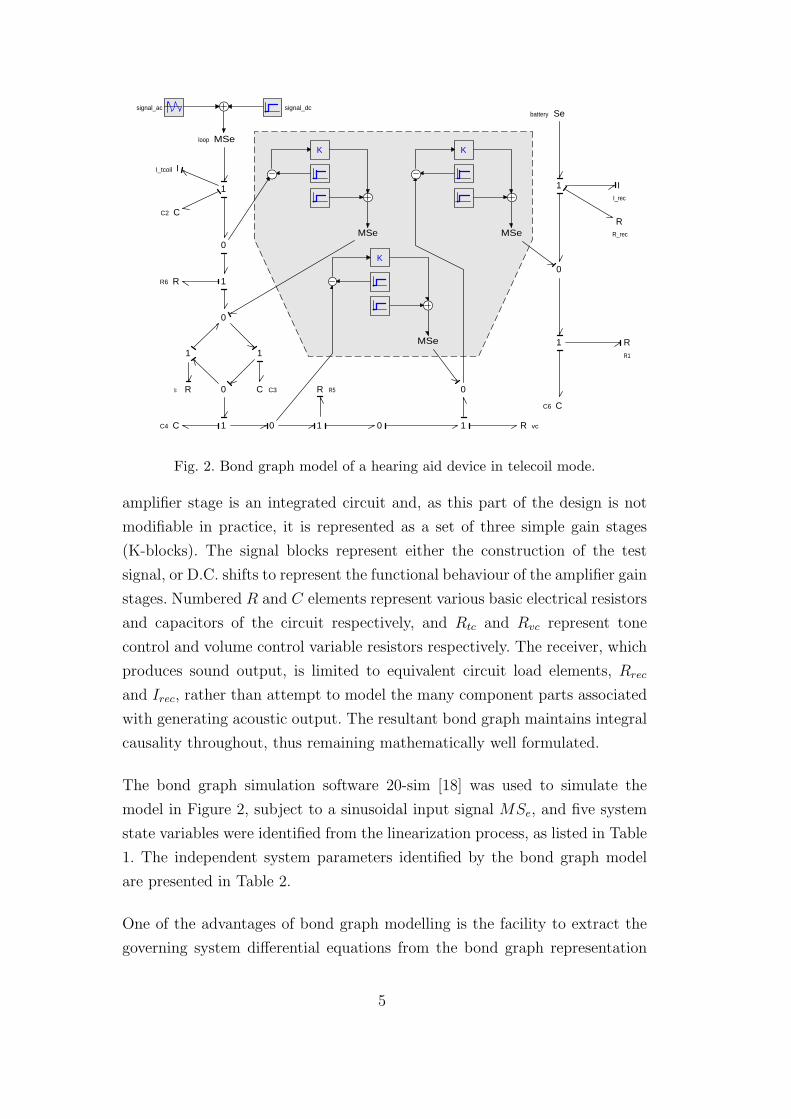
Figure 2 shows the bond graph model of the BTE hearing aid device which
in this paper is modelled in telecoil mode rather than microphone mode as
considered in [5]. In the bond graph representation, the telecoil is represented
as a pure inductance by a generalised inertia element, Itcoil. Indeed, all the
electro-magneto-mechanical elements are represented in electrical terms in this
bond graph in accordance with standard industry practice. The signal to the
telecoil originates from a radio loop, which is represented as a modulated
effort source with a.c. and d.c. parts. The three-stage amplifier is prominent
in the center of the bond graph (shaded grey) is represented here, as in [5],
in signal terms rather than power transmitting elements. This is because the
4
1
1
11
11
1
RR_rec
Rtc
R vc
R R5
RR6
0
0
0
0
0
0
0
CC2
CC6
CC4
C C3
signal_ac signal_dc
MSeloop
MSe
MSe
MSe
Sebattery
II_tcoil
II_rec
K
K
K
1 RR1
1
Fig. 2. Bond graph model of a hearing aid device in telecoil mode.
amplifier stage is an integrated circuit and, as this part of the design is not
modifiable in practice, it is represented as a set of three simple gain stages
(K-blocks). The signal blocks represent either the construction of the test
signal, or D.C. shifts to represent the functional behaviour of the amplifier gain
stages. Numbered R and C elements represent various basic electrical resistors
and capacitors of the circuit respectively, and Rtc and Rvc represent tone
control and volume control variable resistors respectively. The receiver, which
produces sound output, is limited to equivalent circuit load elements, Rrec
and Irec, rather than attempt to model the many component parts associated
with generating acoustic output. The resultant bond graph maintains integral
causality throughout, thus remaining mathematically well formulated.
The bond graph simulation software 20-sim [18] was used to simulate the
model in Figure 2, subject to a sinusoidal input signal MSe, and five system
state variables were identified from the linearization process, as listed in Table
1. The independent system parameters identified by the bond graph model
are presented in Table 2.
One of the advantages of bond graph modelling is the facility to extract the
governing system differential equations from the bond graph representation
5

vC2(t) Voltage across C2
vC3(t) Voltage across C3
vC4(t) Voltage across C4
irec(t) Current through Receiver
itcoil(t) Current through TelecoilTable 1
System states in bond graph of hearing aid system
by linearization around a working point, determined by solving the nonlinear
system and specifying system inputs and outputs. This is achieved by enforc-
ing conservation of power laws at each junction in terms of the independent
effort and flow variables, and is performed automatically by the bond graph
simulation software [18]. The linearized dynamic governing system differential
equations of the system in Figure 2 are generated by the bond graph simulator
and written in matrix form as follows.
v′C2
v′C3
v′C4
i′rec
i′tcoil
=
0 0 0 0 1C2
0 − R5+Rvc+8Rtc
C3Rtc(R5+Rvc)−8
C3(R5+Rvc)0 R6(R5+Rvc−23.2Rtc)
4C3Rtc(R5+Rvc)
0 −8C4(R5+Rvc)
−8C4(R5+Rvc)
0 −5.9R6
C4(R5+Rvc)
0 305.1Irec
305.1Irec
−Rrec
Irec
225.9R6
Irec
−1Itcoil
0 0 0 −1.738R6
Itcoil
vC2
vC3
vC4
irec
itcoil
+
0
0
0
0
MSe
Itcoil
(1)
Here u′ denotes a derivative of u with respect to time and numerical values
represent the substitution of numerical constants such as amplifier gain and
battery voltage in the model. A member of the ODE suite of codes in MAT-
LAB [19] was modified to solve the dynamic system (1) and this solution was
compared against that of bond graph software simulator [18] to validate the
accuracy of the extracted linear equation system. The accuracy of the bond
graph representation has already been validated against experimental results
in [5] for the microphone mode.
6

3 Sensitivity and Uncertainty Analysis
3.1 General Theory
First order dynamic differential models such as (1), linear or otherwise, take
the general formdy
dt= f(y, θ, t) (2)
where t represents time, y and θ represent the vectors containing the n sys-
tem outputs (solutions) and m parameters respectively, and f is a vector
of functions in y, θ and t such that y = [y1, y2, ..., yn]T , θ = [θ1, θ2, ..., θm]T
and f = [f1, f2, ..., fn]T . Note that when f(y, θ, t) can be broken into a pure
state and a forcing input, as in the present case, we may write f(y, θ, t) =
f(y, θ, t) + u(θ, t). Taking derivatives with respect to θ on either side of the
governing equations (2) results in the sensitivity differential equations
dS(θ, t)
dt=
∂f
∂yS(θ, t) +
∂f
∂θ(3)
which describe the time evolution of the n×m local sensitivity matrix S(θ, t)
whose components are given by
Sij =∂yi(θ, t)
∂θj
(4)
The components (4) are termed local sensitivity coefficients. In (3), the
n× n matrix ∂f∂y
and n×m matrix ∂f∂θ
can be derived explicitly from (2) and
are termed the Jacobian and parametric Jacobian matrices respectively.
By the direct method for sensitivity analysis [20] [21] the sets of differential
equations (2) and (3) are solved jointly at each time step of a numerical time
integration scheme, with information generated in the solution of (2) used
in the solution of (3). Accordingly a solution to both y(θ, t) and S(θ, t) is
returned at each time step of the numerical method. In the work presented
here a member of the ODE suite of codes ode45 [22] in MATLAB was modified
to solve the governing and sensitivity differential equation system in this way.
Whilst numerical methods are not necessarily required to solve a linear gov-
erning system, the direct method as outlined here is readily extendable to
7

more complex non-linear models. At any time point t0 during the numerical
solution process, based on a first order Taylor series approximation [23], the
covariance of the system output vector cov(y) can be approximated by
cov(y(t0)) ≈ S(µθ, t0)ΣθST (µθ, t0) (5)
where Σθ is the covariance matrix based on the predetermined variability in
the system parameters and µθ is the vector of nominal parameter values. For
independent system parameters θi such that
Σθ = diag(σ2(θ1), .., σ2(θm)) (6)
a linear estimate of σ2(yi(t0)), the variance of model output yi at t0 owing to
parameter variability, can be written from (5) as
σ2(yi(t0)) =m∑
j=1
σ2j (yi) (7)
where σ2(yi(t0)) represents the diagonal elements of cov(y(t0)), and
σ2j (yi) ≈ S2
ij(µθ, t0)σ2(θj) (8)
is the contribution of the variance σ2(θj) in parameter θj to the resultant vari-
ance in model output yi at t0. Therefore, the total output variance represented
in equation (7) is a sum over independent parameter contributions.
3.2 Telecoil Sensitivity Formulation
Following on from the theory in section 3.1, for the telecoil system the state
and parameter vectors are given from Tables 1 and 2 respectively by
y = [vC2 , vC3 , vC4 , irec, itcoil]T (9)
θ = [Itcoil, R6, Irec, Rrec, C2, C4, R5, Rvc, C3, Rtc]T (10)
and the functions contained in the vector f of equation 2 are defined by the
matrix-vector multiplication on the right hand side of (1).
8

The parametric Jacobian matrix in equation (3) is thus defined as
∂f
∂θ=
0 0 0 0∂v′
C2
∂C20 0 0 0 0
0∂v′
C3
∂R60 0 0 0
∂v′C3
∂R5
∂v′C3
∂Rvc
∂v′C3
∂C3
∂v′C3
∂Rtc
0∂v′
C4
∂R60 0 0
∂v′C4
∂C4
∂v′C4
∂R5
∂v′C4
∂Rvc0 0
0 ∂i′rec
∂R6
∂i′rec
∂Irec
∂i′rec
∂Rrec0 0 0 0 0 0
∂i′tcoil
∂Itcoil
∂i′tcoil
∂R60 0 0 0 0 0 0 0
(11)
whose elements should not be taken literally, but can be derived analytically
from (1) as presented in Appendix A (known zeros are indicated). Owing to
system linearity, the Jacobian ∂f∂y
for the hearing aid system is equivalent to
the system matrix in (1).
Solving the formulated sensitivity equation in the form of (3) alongside the
governing system (1) returns the values of the system solution variables at
each time step along side the sensitivity coefficients of equation (4) which
form system sensitivity matrix given in this application by
S(µθ, t) =
∂vC2
∂Itcoil
∂vC2
∂R6
∂vC2
∂Irec
∂vC2
∂Rrec
∂vC2
∂C2
∂vC2
∂C4
∂vC2
∂R5
∂vC2
∂Rvc
∂vC2
∂C3
∂vC2
∂Rtc
∂vC3
∂Itcoil
∂vC3
∂R6
∂vC3
∂Irec
∂vC3
∂Rrec
∂vC3
∂C2
∂vC3
∂C4
∂vC3
∂R5
∂vC3
∂Rvc
∂vC3
∂C3
∂vC4
∂Rtc
∂vC4
∂Itcoil
∂vC4
∂R6
∂vC4
∂Irec
∂vC4
∂Rrec
∂vC4
∂C2
∂vC4
∂C4
∂vC4
∂R5
∂vC4
∂Rvc
∂vC4
∂C3
∂vC4
∂Rtc
∂irec
∂Itcoil
∂irec
∂R6
∂irec
∂Irec
∂irec
∂Rrec
∂irec
∂C2
∂irec
∂C4
∂irec
∂R5
∂irec
∂Rvc
∂irec
∂C3
∂irec
∂Rtc
∂itcoil
∂Itcoil
∂itcoil
∂R6
∂itcoil
∂Irec
∂itcoil
∂Rrec
∂itcoil
∂C2
∂itcoil
∂C4
∂itcoil
∂R5
∂itcoil
∂Rvc
∂itcoil
∂C3
∂itcoil
∂Rtc
(12)
where each of the coefficients in (12) are calculated at µθ and at time t, where
µθ is determined using the nominal values of the system parameters. The
parameter nominal values and manufacturing tolerances for the hearing aid
design were taken from the manufacturers data sheets and are presented in
Table 2. Each manufacturing tolerance acts as a source of variability that is
translated to variation in the system output. Parameter standard deviation
was computed by assuming all parameter values are uniformly distributed
within the prescribed range and using the standard formula σ = (b−a)/(2√
3),
where a and b are the lower and upper bounds, respectively.
9

parameter description nominal tolerance Std. Dev.
R5 resistance R5 6800 Ω ±10% 392.6 Ω
R6 resistance R6 75000 Ω ± 5% 2165 Ω
Rrec receiver resistance 500 Ω ±10% 28.87 Ω
Rtc tone control resistance 1700 Ω ±10% 98.14 Ω
Rvc volume control resistance 50000 Ω ±20% 5774 Ω
C2 capacitance C2 100e-09 F ± 5% 2.887e-09 F
C3 capacitance C3 15e-09 F ±10% 0.866e-09 F
C4 capacitance C4 0.47e-06 F +80% -20% 0.137e-06 F
Irec receiver inductance 0.345 H ±22% 0.0438 H
Itcoil telecoil inductance 0.295 H ±15% 0.0255 HTable 2
Hearing aid system parameter descriptions, manufacturing data for nominal values
and tolerances and calculated standard deviations assuming Uniform distribution.
Using the sensitivity matrix (12) variations in parameter value can be prop-
agated through to the system output using equations (7) and (8), with the
individual sources contributing most to the output variance being identified
by (8). The results of numerically implementing this strategy for determining
the sources of variability in the hearing aid system model output are presented
in Section 4.
4 Numerical Results
From the system outputs listed in Table 1, the currents irec and itcoil are
investigated in terms of their sensitivity to other circuit component values
since, in telecoil mode, the telecoil and receiver are known to interact in close
proximity [24]. At a sinusoidal input signal 2 of amplitude 1mV and frequency
1 kHz, the simulated solutions irec and itcoil generated by solving the governing
differential system (1) using a time integration scheme are also 1 kHz sinusoids
2 This signal is equivalent to the expected input generated by a telecoil.
10

parameter σj(irec) σj(itcoil)
R5 0.09e-06 0
R6 0.67e-06 224.3e-12
Rrec 0.91e-06 0
Rtc 0.37e-06 0
Rvc 1.44e-06 0
C2 0.02e-06 2.7e-12
C3 0.41e-06 0
C4 0.78e-06 0
Irec 8.79e-06 0
Itcoil 0.09e-06 28.7e-12
Table 3
Individual parameter contribution to output sensitivity, expressed as standard de-
viations (Amperes per unit change of jth parameter).
of varying amplitudes with a d.c. offset. The system sensitivity coefficients
will also be periodic at the same frequency since the governing and sensitivity
equation systems share the same eigenvalues. By using the system sensitivity
coefficients computed at each step of the solution procedure, the parameter
variances were propagated through to the chosen model outputs. The peak-
to-peak amplitudes of the simulated sinusoid solutions irec and itcoil, and their
corresponding variances due to variation in parameter values are presented in
Tables 3 and 4.
The output variance in itcoil was found to be mostly due to the variance of
R6, although this variance is negligible compared to the nominal output value
of itcoil. As such itcoil can be considered robust to parameter variations. The
major contributor to the variance in irec was seen to be that of parameter Irec
alongside small contributions from parameters Rvc, Rrec, C4 and R6. As such,
manufacturing tolerances on the other parameters have little or no effect on
system performance.
11
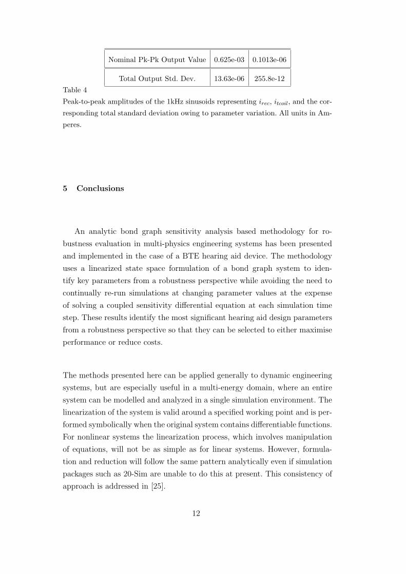
Nominal Pk-Pk Output Value 0.625e-03 0.1013e-06
Total Output Std. Dev. 13.63e-06 255.8e-12Table 4
Peak-to-peak amplitudes of the 1kHz sinusoids representing irec, itcoil, and the cor-
responding total standard deviation owing to parameter variation. All units in Am-
peres.
5 Conclusions
An analytic bond graph sensitivity analysis based methodology for ro-
bustness evaluation in multi-physics engineering systems has been presented
and implemented in the case of a BTE hearing aid device. The methodology
uses a linearized state space formulation of a bond graph system to iden-
tify key parameters from a robustness perspective while avoiding the need to
continually re-run simulations at changing parameter values at the expense
of solving a coupled sensitivity differential equation at each simulation time
step. These results identify the most significant hearing aid design parameters
from a robustness perspective so that they can be selected to either maximise
performance or reduce costs.
The methods presented here can be applied generally to dynamic engineering
systems, but are especially useful in a multi-energy domain, where an entire
system can be modelled and analyzed in a single simulation environment. The
linearization of the system is valid around a specified working point and is per-
formed symbolically when the original system contains differentiable functions.
For nonlinear systems the linearization process, which involves manipulation
of equations, will not be as simple as for linear systems. However, formula-
tion and reduction will follow the same pattern analytically even if simulation
packages such as 20-Sim are unable to do this at present. This consistency of
approach is addressed in [25].
12

Appendix A
The elements of the parametric Jacobian matrix of equation 11 are given by
∂v′C2
∂C2
=−itcoil
C22
(13)
∂v′C3
∂C3
=vC3(8Rtc + R5 + Rvc) + R6itcoil(5.8Rtc − 0.26(R5 + Rvc)) + 8RtcvC4
C23Rtc(R5 + Rvc)
(14)∂v′C3
∂R5
=∂v′C3
∂Rvc
=8vC3 + 8vC4 + 5.9R6itcoil
C3(R5 + Rvc)2(15)
∂v′C3
∂Rtc
=vC3 − (R6itcoil)/4
C3R2tc
(16)
∂v′C3
∂R6
=−5.9itcoil
C3(R5 + Rvc)(17)
∂v′C4
∂C4
=(8vC3 + 8vC4 + 5.9R6itcoil)
C24(R5 + Rvc)
(18)
∂v′C4
∂R5
=∂v′C4
∂Rvc
=8vC3 + 8vC4 + 5.9R6itcoil
C4(R5 + Rvc)2(19)
∂v′C4
∂R6
=−5.9itcoil
C4(R5 + Rvc)(20)
∂i′rec
∂Irec
=1
I2rec
(−305vC3 − 305vC4 + Rrecirec − 226R6itcoil) (21)
∂i′rec
∂Rrec
=−irec
Irec
(22)
∂i′rec
∂R6
=226itcoil
Irec
(23)
∂i′tcoil
∂Itcoil
=1
I2tcoil
(vC2 + 1.73itcoilR6 −MSe) (24)
∂i′tcoil
∂R6
=−1.73itcoil
Itcoil
(25)
Acknowledgements
The authors wish to thank Siemens Hearing Instruments Ltd, Crawley, UK for
access to their hearing aid manufacturing data. This work was supported by
the Engineering & Physical Sciences Research Council (EPSRC) at the Lon-
don School of Economics under grant number GR/S63502/01 and at Brunel
University under grant number GR/S63496/02.
13

References
[1] J. Wu and M. Hamada. Experiments: Planning, Analysis, and Parameter
Design Optimization. Wiley, 2000.
[2] D. M. Grove and T. P. Davis. Engineering, Quality and Experimental Design.
Longman, 1992.
[3] T.R. Hsu. MEMS and Microsystems: Design and Manufacture. McGraw-Hill
Company, Boston, 2002.
[4] B. Shield. Evaluation of the social and economic costs of hearing impairment.
www.hearit.org, 2005.
[5] M. A. Atherton, R.A. Bates, D. Ashdown, and F. Jensen. Evaluating hearing
aid robustness using bond graph models. Proc. of Mechatronics 2002, 24-26
June, Enchede, Netherlands, pages 591–597, 2002.
[6] H. Kim and D. Barrs. Hearing aids: A review of whats new. Otolaryngology -
Head and neck surgery, 134:1043–1050, 2006.
[7] J. Gao, H. Zhang, and G. Hu. Real time implementation of an efficient
speech enhancement algorithm for digital hearing aids. Tsinghua Science and
Techmology, 11(2):475–480, 2006.
[8] H. Puder. Adaptive signal processing for interference cancellation in hearing
aids. Signal Processing, 86:1239–1253, 2006.
[9] J-B. Maj, L. Royackers, J. Wouters, and M. Moonen. Comparison of
adaptive noise reduction algorithms in dual microphone hearing aids. Speech
Communication, 48:957–970, 2006.
[10] H.M. Paynter. Analysis and Design of Engineering Systems. MIT Press,
Cambridge, MA., 1961.
[11] D.C. Karnopp. Computer simulation of stick-slip friction in mechanical dynamic
systems. Transcepts of ASME Journal of Dynamic Systems, Measurement, and
Control, 107(1):100–103, 1985.
[12] R.C. Rosenberg. Exploiting bond graph causality in physical systems models.
Journal of Dynamic Systems, Measurement, and Control, 109(4):378–383, 1987.
[13] F.E. Cellier. Hierarchical nonlinear bond graphs: a unified methodology for
modelling complex physical systems. Proceedings of European Simulation
Multiconference on Modelling and Simulation, pages 1–3, 1990.
14

[14] D.C. Karnopp. Energetically consistent bond graph models in electromechanical
energy conversion. Journal of the Franklin Institute, 325(7):667–686, 1990.
[15] M.A. Atherton and R.A. Bates. Bond graph analysis in robust engineering
design. Quality and Reliability Engineering International, 16:325–335, 2000.
[16] P. J. Gawthrop. Sensitivity bond graphs. Journal of the Franklin Institute,
227:907–922, 2000.
[17] W. Barutski and J. Granda. Bond graph based frequency domain sensitivity
analysis of multidisciplinary systems. Proceedings of the I MECH E Part I:
Journal of Systems & Control Engineering, 216(1):85–99, 2002.
[18] Controllab Products B. V. http://www.20sim.com.
[19] L. F. Shampine and M. W. Reichelt. The matlab ode suite. Siam Journal of
Scientific Computing, 18(1):1–22, 1997.
[20] J. R. Leis and M. A. Kramer. The simultaneous solution and sensitivity analysis
of systems described by ordinary differential equations. ACM Transactions on
Mathematical Software, 14(1):45–60, 1988.
[21] A. M. Dunker. The decoupled direct method for calcuating sensitivity
coefficients in chemical kinetics. J. Chem. Phys, 81:2385–2393, 1984.
[22] L. F. Shampine and M. W. Reichelt. The matlab ode suite. Siam J. Sci.
Comput., 18(1):1–22, 1997.
[23] Dan G. Cacuci. Sensitivity and Uncertainty Analysis Theory. Chapter 3,
Chapman and Hall/CRC, 2003.
[24] Y. Shen, M. A. Perry, E. Kaymak, M. A. Atherton, R. A. Bates, and H. P.
Wynn. Experimental and bond graph based sensitivity calculations for micro
scale robust engineering design. Annecy, France 2005: Research and Education
in Mechtronics, pages CD–ROM, 2005.
[25] D.C. Karnopp, D.L. Margolis, and R.C. Rosenberg. System Dynamics, pages
138–142. Wiley Interscience, 1990.
15