Bond and Foreign Exchange Risk Premia∗

Serhiy Kozak†

January 30, 2011

Abstract

This paper explores the relationship between bond and foreign exchange risk premia. I

extend the Cochrane and Piazzesi [2005] results across countries and for longer maturities. I

show that cross country bond risk premia are correlated and extract the global bond Cochrane-

Piazzesi factor (GCP). Excess returns on bonds of each country are modeled using two factors:

GCP and a country speci�c one. Excess foreign exchange returns are modeled using two factors

as well: the average interest rate di�erential (home country speci�c factor, AD) and the global

carry trade factor. I further show that the global carry trade and GCP factors are related. AD

and GCP factors predict excess foreign exchange returns and their relative importance changes

with the currency risk (as measured by forward spread). Finally, I present a long-run risk model

that motivates the use of two factors in explaining foreign exchange excess returns.

∗I thank John Cochrane, Eugene Fama, Lars Hansen, John Heaton and my classmates at Chicago Booth forhelpful comments and suggestions.†Booth School of Business and Department of Economics, University of Chicago. Email: kozak@chicagobooth.edu.

The latest version is available at http://home.uchicago.edu/skozak

1

1 Introduction

The paper explores the relationship between risk premia in bond and foreign exchange markets.

The two markets are closely linked: investing in foreign bonds often implies loading on currency

risk. Using available �nancial instruments these two risks, however, can be decomposed into two

independent pieces: pure bond risk premium and pure foreign exchange risk premium. This decom-

position requires only that the currency forwards markets exist and are e�cient. I show that excess

returns on foreign bonds in foreign currency are approximately equal to excess returns on foreign

bonds in home currency hedged by participating in forwards markets.

While the decomposition allows us to study two markets separately, it is important to understand

how these two markets interact and whether they have common risk structure or can be hedged by

each other. This paper is the �rst step towards understanding this question.

I �rst start with extending Cochrane and Piazzesi [2005] results in the US by including forward

rates 6 through 10 in their regressions. The Cochrane-Piazzesi (CP) factor turns out to be very

robust and fully preserves the 1-5 forward rates structure while displaying an additional dip at a

loading on 8th year forward rate. Including 10 forwards raises an issue of over�tting in a small

sample. I propose an empirical strategy to verify whether including additional lags in the regression

does indeed outperform original Cochrane and Piazzesi [2005] regression in short sample.

I then extend the analysis of bond markets to di�erent countries. Cochrane and Piazzesi [2005]

showed that the single factor can predict bond excess return in the US at all maturities. This

factor is correlated with the US business cycle and hence is a good candidate for a risk premium

variable. Several papers (Kessler and Scherer [2009], Dahlquist and Hasseltoft [2010]) attempted

to extend the results of Cochrane and Piazzesi [2005] to other countries, but did not succeed. I

show that the problem lies in the data the papers use: they rely on yield curve datasets which are

smoothed across maturities. The Cochrane and Piazzesi [2005] regression estimates rely on multiple

di�erencing of yields, and thus yield curve smoothing can destroy the very information being looked

for. The authors themselves use unsmoothed Fama and Bliss [1987] yields and hence preserve this

information. As a result, Cochrane and Piazzesi [2005] �nd an attractive tent-shaped pattern of

loadings in their paper, while the other two papers mentioned lose this pattern altogether.

To deal with the data issues I propose using interest rate swaps dataset to estimate the CP

factor in other countries. The yields derived from interest rate swaps are not precisely zero-coupon

yields due to embedded default premium (through their dependence on the LIBOR rate). They turn

out, however, to produce better estimates of zero-coupon bond yields than the yields calculated by

Diebold and Li [2006], who employ the Fama and Bliss [1987] methodology to the actual bond

data. Interest rate swap rates are traded every day and thus do not have to be approximated by

other instruments with similar maturities. Moreover, the Fama and Bliss [1987] methodology has

di�culties with the current crisis period which can be avoided by using swaps data.

By using interest rate swaps I �nd similar tent-shaped factors in the UK, Germany, Japan and

Switzerland. The �nding suggests that CP factor is also robust across countries. CP factors in

�ve countries are correlated. Moreover, CP factors from foreign countries often help to predict

2

bond excess returns in the home country. I perform multiple tests to see how foreign risk premia

are related and a�ect each other. I also �nd that a common component of all CP factors is an

important predictor of risk premia in each country and can hence serve as a global risk factor. The

central question is whether and how this risk is related to foreign exchange market risks.

I further investigate foreign exchange market predictability. To focus on the risk premia story

and minimize the noise in foreign exchange data, I work with forward-spot spread (or interest rate

di�erential) sorted portfolios of currencies, similar to Lustig and Verdelhan [2007], Lustig et al.

[2010a].

Lustig et al. [2010a] �nd that two factors explain the cross-section of foreign exchange returns.

Evidence on time-series predictability in foreign exchange market, however, are weak. Hansen and

Hodrick [1980], Fama [1984] were the �rst to show that foreign exchange returns are predictable and

hence time-varying risk premia story is plausible. There are several potential sources of time-varying

risk premia in foreign exchange market. One is related to the Lustig et al. [2010a] level factor in

the cross-section � the risk associated with the home country's currency movements. The other is

the global risk of di�erential investment in one country vs. another (related to cross-section slope

factor) � carry trade as a special case. This risk premium can also be time-varying. Lustig et al.

[2010a] showed that by sorting countries in portfolios and looking at the di�erences in returns of one

portfolio vs. another, we are able to isolate common innovations to the stochastic discount factor

(SDF).

The choice of common and individual risk factors is consistent with the �ndings in the literature.

Backus et al. [2001] �nd that we need large common component with di�erential loadings to explain

foreign exchange market anomalies. Brandt et al. [2006] document that large common component

is necessary to explain relatively low foreign exchange market volatility (relative to stock market).

This motivates the global risk factor in foreign exchange markets. Similarly, all exchange rates move

together when home country appreciates or depreciates. This home country currency movement

requires including a country speci�c risk factor.

I therefore �nd two factors to be important in explaining the time-series of foreign exchange

returns. The average interest rate di�erential (AD) serves as a US-speci�c factor. It is signi�cant

for countries with low interest rates that face little risk of depreciation, but loses signi�cance in

countries with high interest rates. These countries, however, have signi�cant negative slopes on the

GCP factor, while the countries with low interest rates have insigni�cant slopes. In this story, the

carry trade strategy should be free of US-speci�c risk and load on global carry trade factor. I �nd

that excess returns on carry trade load signi�cantly on the GCP factor which means that global

carry-trade and GCP factors are related. AD factor, however, has marginal predictive power on

carry trade excess returns as well, which suggests that GCP does not fully capture foreign exchange

global factor. AD has large global component and its ability to predict carry trade excess returns

comes through this channel.

The two factor approach allows us to link foreign exchange risk premium to that of bonds.

Indeed, bond risk premium can be modeled using two factors as well: a global Cochrane-Piazzesi

3

(GCP) factor and a country-speci�c CP factor. Bond market's GCP factor seems like a direct equiv-

alent of foreign exchange market's carry trade factor. Country-speci�c bond and foreign exchange

factors can be connected too. In terms of the risk premium macro story, we can expect global risk

factors be related to global business cycles while country-speci�c factors re�ect a country-speci�c

business cycle risk (net of global).

Finally, I present a long-run risk model that motivates the use of two factors in explaining

foreign exchange excess returns. The model features Epstein and Zin [1989] preferences together

with long-run predictable component in consumption as in Bansal and Yaron [2004]. Both the

consumption growth conditional variance and conditional variance of expected consumption growth

are conditionally heteroskedastic. In addition, it is assumed that long-run predictable consumption

components are perfectly correlated across countries, while short-run news are i.i.d. The model

implies that the bond risk premia in each country is driven by conditional volatility of expected

consumption growth only. Therefore, if we believe that CP factor is a good proxy for expected

bond returns, we might use it to recover the conditional volatility. Expected currency excess returns

depend on both volatilities. It is further shown, that they can be recovered in a similar way using

AD and GCP factors.

2 Bond risk premia

Bond risk premia move over time. Cochrane and Piazzesi [2005] �nd a single factor that predicts

US bonds excess returns on one- to �ve-year maturities. This factor is a tent-shaped linear function

of �ve forward rates.

In this section I reproduce Cochrane and Piazzesi [2005] results at 5 year maturity and extend

them to maturities up to 10 years. I estimate CP factor in di�erent datasets and con�rm Cochrane

and Piazzesi [2009] claim that CP factor should be estimated using unsmoothed yields data.

I further estimate CP factors in four additional countries: UK, Japan, Germany and Switzerland.

The estimates suggest the same single factor structure with roughly the same shape in all countries.

To my knowledge this is a new result in the literature. Several papers, namely Dahlquist and

Hasseltoft [2010], Kessler and Scherer [2009], estimated CP factors in the same set of countries

but did not �nd anything like the tent-shaped factor as in Cochrane and Piazzesi [2005]. These

seemingly contrary results are explained by the di�erences in data used: both papers estimate the

CP factor out of smoothed zero-coupon yield curve datasets (either Datastream or Central Banks

of individual countries). In fact, using the same data as they do, I con�rm that the estimates of

CP factor are nothing but noise � huge negative and positive alternating loadings on forwards are

a clear sign of enormous multicollinearity problem.

I follow Cochrane and Piazzesi [2005] notation. Let p(n)t denote log price of n-year discount

bond at time t. Yields are given by y(n)t = − 1

np(n)t . Forward rate from t + n − 1 to t + n is then

fnt = p(n−1)t − pnt . Bond excess returns are de�ned as

4

brxnt+1 = br(n)t+1 − y

(1)t

= p(n−1)t+1 − p(n)

t − y(1)t

2.1 US data

2.1.1 Cochrane and Piazzesi [2005] speci�cation

Cochrane and Piazzesi [2005] �nd a single factor to forecast bond risk premia. Their factor is a

linear combination of �ve forward rates.

brx(n)t+1 = bn

(γ0 + γ1yt + γ2f

(2)t + ...+ γ5f

(5)t

)+ ε

(n)t+1

They use a dataset constructed using Fama and Bliss [1987] methodology and available from

CRSP. I replicate their result using the same data in panel (A) of Figure 1. The sample is from

1965 till 2005. All loadings have the usual tent-shaped pattern. Simple factor structure looks like

a reasonable restriction and is further veri�ed by the eigen-value decomposition of the covariance

matrix of expected returns. The �rst principal component in such decomposition accounts for more

than 99% of the variance. The �tted single factor constructed as in Cochrane and Piazzesi [2005]

is shown with the dotted line on the plot.

Panel (B) plots the loadings of excess bond returns on �ve forwards in the subsample of 1987-

2005. We see that the single factor tends to lose its shape as the size of the sample decreases. While

the general tent shape can still be observed, the factors load much more heavily on positive/negative

positions, which re�ects the multicollinearity issue in a small sample.

Panel (C) depicts the construction of CP factor using Gürkaynak et al. [2007] data. In con-

structing the yield curve, they follow the extension by Svensson [1994] of Nelson and Siegel [1987]

approach by assuming that the instantaneous forward curve can be parametrized by six parameters

according to the following functional form

ft(n, 0) = β0 + β1exp

(− nτ1

)+ β2

(− nτ1

)exp

(− nτ1

)+ β3

(− nτ2

)exp

(− nτ2

)Panel (C) shows that the factor loses its shape and predictive power altogether. Cochrane and

Piazzesi [2009] argue that this is due to data smoothing, which is insigni�cant for most of the

purposes, but a�ects the results when multiple di�erencing of data is performed. In our case, excess

returns and forward rates are di�erences of yields. Including multiple forward rates introduces even

further di�erencing by the means of OLS mechanics.

I use three additional datasets to test robustness of the CP factor in alternative samples. The �rst

one uses the yields on discount bonds inferred from interest rate swaps available from Datastream1.

1Interest rate swaps exchange a �oating stream of payments for a �xed one. Fixed interest is paid either annuallyor semi-annually, depending on the country. All interest payments are discounted to period zero using a proper

5

Figure 1: US CP factor, di�erent datasets and subsamples

1 2 3 4 5−4

−2

0

2

4

6(C) GSW, 1965−2005

1 2 3 4 5

−2

0

2

4(E) Diebold, 1970−2000

1 2 3 4 5−2

−1

0

1

2(F) DLY, 1985−2005

1 2 3 4 5

−2

0

2

4

6

(B) Fama−Bliss, 1987−2005

1 2 3 4 5

−2

0

2

4(A) Fama−Bliss, 1965−2005

1 2 3 4 5−5

0

5

10

(D) Swaps, 1987−2005

The �gure shows the loadings of bond excess returns at various maturities on �ve forward rates. These are the

coe�cients γ in the regression brx(n)t+1 = bn

(γ0 + γ1yt + γ2f

(2)t + ...+ γ5f

(5)t

)+ ε

(n)t+1. Each line corresponds to a

di�erent maturity. Loadings increase linearly in maturity and thus the lowest variance line corresponds to maturityof two years, while the highest � to ten years. The dotted line with a triangular marker shows the extracted CP factorloadings. Plot (A) replicates the results of Cochrane and Piazzesi [2005] by using Fama and Bliss [1987] dataset from1965 to 2005. Plot (B) show results for the subsample of Fama and Bliss [1987] rates. Plot (C) uses Gürkaynak et al.[2007] data (1965-2005). Plot (D) uses interest rate swaps data from Datastream (1987-2005). Plot (E) uses Dieboldand Li [2006] dataset. The last plot (F) shows the estimates for Diebold et al. [2007] dataset.

6

The resulting yields are not exactly the same as yields on zero-coupon bonds, since they also

include interest rate swap spreads (see Fehle [2003] or Du�e and Singleton [1997] for more technical

discussion). The main driver of the di�erence is that interest rate swaps typically use LIBOR as a

�oating reference rate, but LIBOR re�ects a default premium. The di�erence between zero-coupon

and interest rate swap yields, however, is not very signi�cant empirically, and using swaps seems

like a reasonable approximation. One important bene�t of interest swap data is that it is much

�cleaner� � interest rate swap rates are traded every day and thus do not have to be approximated

by other instruments with similar maturities. Panel (D) illustrates the CP factor extracted from

swaps. While the factor seems to lose a usual tent shape, it does look like a magni�ed version of

Fama-Bliss CP factor in 1987-2005 data sample.

Another dataset is constructed by Diebold and Li [2006] and is available on Francis Diebold's

website. Diebold and Li [2006] use Fama-Bliss unsmoothed approach to estimate yields on zero-

coupon bonds. Unlike the Gürkaynak et al. [2007] procedure, forward curve is not approximated

by a Svensson [1994] functional form; instead, all the yields are extracted by back-substitution and

proper discounting. As a result, this delivers similar tent-shaped pattern as with original CRSP

Fama-Bliss data. Panel (E) shows the loadings.

The last dataset comes from Diebold et al. [2007]2. The factor constructed from this dataset

seems to have problems with the �fth coe�cient, but the rest are generally consistent with the

tent-shape pattern.

2.1.2 Longer maturities

Cochrane and Piazzesi [2005] use only forward rates up to 5 years in their analysis. It is mostly due

to data availability issue: Fama and Bliss [1987] yields on zero-coupon bonds are limited to only 5

years in maturity. Cochrane and Piazzesi [2009] add longer maturities by utilizing Gürkaynak et al.

[2007] dataset. They mention, however, that the yields are smoothed and therefore the information

in forward rates might be lost. Indeed, they �nd that adding forward rates beyond 5 Fama and

Bliss [1987] rates introduces plenty of multicollinearity and has almost no improvement in terms of

R2.

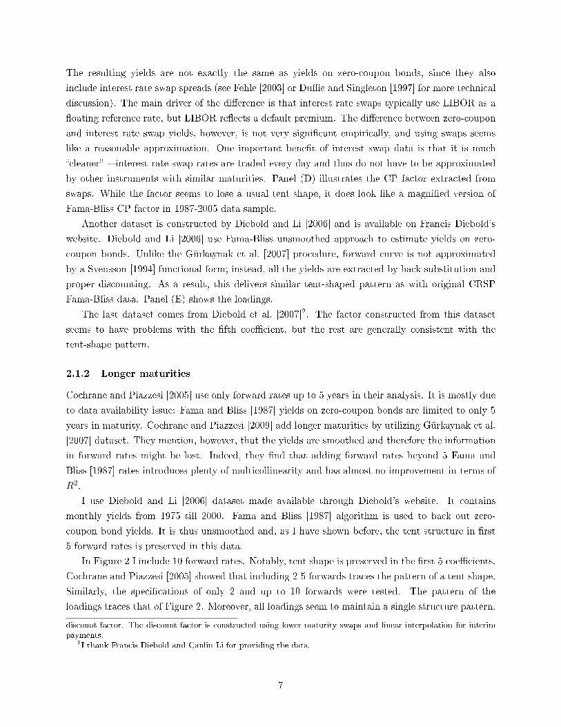
I use Diebold and Li [2006] dataset made available through Diebold's website. It contains

monthly yields from 1975 till 2000. Fama and Bliss [1987] algorithm is used to back out zero-

coupon bond yields. It is thus unsmoothed and, as I have shown before, the tent structure in �rst

5 forward rates is preserved in this data.

In Figure 2 I include 10 forward rates. Notably, tent shape is preserved in the �rst 5 coe�cients.

Cochrane and Piazzesi [2005] showed that including 2-5 forwards traces the pattern of a tent shape.

Similarly, the speci�cations of only 2 and up to 10 forwards were tested. The pattern of the

loadings traces that of Figure 2. Moreover, all loadings seem to maintain a single structure pattern.

discount factor. The discount factor is constructed using lower maturity swaps and linear interpolation for interimpayments.

2I thank Francis Diebold and Canlin Li for providing the data.

7

Figure 2: US CP factor, maturities up to 10 years

1 2 3 4 5 6 7 8 9 10

−6

−4

−2

0

2

4

6

(E) Diebold, 1970−2000

The �gure shows the loadings of bond excess returns at various maturities on ten forward rates. These are the

coe�cients γ in the regression brx(n)t+1 = bn

(γ0 + γ1yt + γ2f

(2)t + ...+ γ10f

(10)t

)+ ε

(n)t+1. Each line corresponds to a

di�erent maturity. Loadings increase linearly in maturity and thus the lowest variance line corresponds to maturityof two years, while the highest � to ten years. The dotted line with a triangular marker shows the extracted factorloadings.

Coe�cients on forwards with maturities above �ve years are signi�cantly lower than those of a tent-

shape. 8-year forward rate seems to be important and is the only statistically signi�cant coe�cient.

This means that risk premium is high when long-horizon forward rate (8 years) is low. 6, 7, 9 & 10th

coe�cients are indistinguishable from zero. We may, however, still want to include some of those to

preserve the single factor structure in data. Figure 3 plots the estimates of CP factor together with

2 standard error bars. Standard errors are adjusted for time-series dependence using Hansen and

Hodrick [1980] approach with an appropriate number of lags3. Newey and West [1987] standard

errors are almost the same. χ2 test strongly rejects the null that coe�cients 6-10 are jointly equal

to zero (p-value is above 0.999).

Figure 4 shows the estimates of coe�cients of excess return regressions on all yields. First �ve

loadings again replicate the results in Cochrane and Piazzesi [2005] (see Figure 2, Panel C in their

paper). The pattern of loadings in this case warns us of potential multicollinearity problems that

might have to be dealt with.

Figure 5 shows loadings of 1, 3, 4, 5, 7, 8 forwards model. I dropped 2-year forward, since it

is not signi�cantly di�erent from zero. Further, forwards 6, 7 are insigni�cant from zero. I drop

the 7th one, but keep the 6th since it helps preserve single factor structure. Everything beyond 8th

year forward rate is dropped as well.

R2 of excess return regressions on various combinations of forwards are reported in Table 1.

3For Hansen and Hodrick [1980] standard errors I use 252 lags for daily data at annual horizon. The number oflags are scaled appropriately for wider horizons. For Newey and West [1987] standard errors (not reported) I used1.5*252 lags for daily data to account for under-weighting of further lags in this estimation technique. For monthlydata and annual horizon 12 and 18 lags were used, correspondingly.

8

Figure 3: US CP factor, 10 forwards, 2 standard errors

1 2 3 4 5 6 7 8 9

−4

−2

0

2

4

6

The �gure shows the loadings of average bond excess returns across maturities on ten forward rates and their standarderrors. These are the coe�cients γ in the regression brx

(n)t+1 = γ0 + γ1yt + γ2f

(2)t + ... + γ10f

(10)t + εt+1. Error bars

depict two standard deviations intervals. Standard errors are Hansen and Hodrick [1980] with an appropriate numberof lags.

Figure 4: US CP factor, loadings on yields, maturities up to 10 years

1 2 3 4 5 6 7 8 9 10

−25

−20

−15

−10

−5

0

5

10

15

20

25

(E) Diebold, 1970−2000

The �gure shows the loadings of bond excess returns at various maturities on ten yields. These are the coe�cients γ in

the regression brx(n)t+1 = bn

(γ0 + γ1yt + γ2y

(2)t + ...+ γ10y

(10)t

)+ ε

(n)t+1. Each line corresponds to a di�erent maturity.

Loadings increase linearly in maturity and thus the lowest variance line corresponds to maturity of two years, whilethe highest � to ten years. The dotted line with a triangular marker shows the extracted factor loadings.

9

Figure 5: US CP factor, selected forwards

1 2 3 4 5 6 7

−4

−2

0

2

4

6

8

The �gure shows the loadings of bond excess returns at various maturities on 1, 3, 4, 5, 6, 8 forward rates. These are

the coe�cients γ in the regression brx(n)t+1 = bn

(γ0 + γ1yt + γ3f

(3)t + ...+ γ8f

(8)t

)+ ε

(n)t+1. Each line corresponds to a

di�erent maturity. Loadings increase linearly in maturity and thus the lowest variance line corresponds to maturityof two years, while the highest � to ten years. The dotted line with a triangular marker shows the extracted factorloadings.

Table 1: Bond excess return forecasts using forwards, R2

brx(2)t+1 brx

(3)t+1 brx

(4)t+1 brx

(5)t+1 brx

(6)t+1 brx

(7)t+1 brx

(8)t+1 brx

(9)t+1 brx

(10)t+1

f1,f3,f5 0.31 0.35 0.35 0.33 0.35 0.31 0.34 0.34 0.30f1-f5 0.34 0.36 0.38 0.36 0.37 0.34 0.37 0.37 0.33

f1,f3,f4,f5,f6,f8 0.38 0.42 0.45 0.43 0.46 0.45 0.43 0.44 0.41f1-f9 0.39 0.43 0.46 0.44 0.47 0.45 0.44 0.44 0.42

f1,f3,f5, MA 0.38 0.42 0.42 0.41 0.43 0.38 0.42 0.40 0.36f1-f5, MA 0.42 0.45 0.46 0.46 0.48 0.44 0.48 0.46 0.41

f1,f3,f4,f5,f6,f8, MA 0.46 0.51 0.53 0.53 0.55 0.53 0.53 0.54 0.51f1-f9, MA 0.47 0.52 0.54 0.55 0.57 0.55 0.54 0.55 0.52

The table reports R2 of bond excess returns regressions on the restricted linear combination of selected forward rates:brx

(n)t+1 = γ

′f t +ε

(n)t+1. f t is constructed as the �rst principal component of the covariance matrix of expected returns.

Each column corresponds to an excess return of di�erent maturity. Each row details which forwards are included informing the factor f t. First 4 rows correspond to the basic speci�cation. The last 4 rows include 3 MA terms of f t

as in Cochrane and Piazzesi [2005].

10

Results with 1-5 forward rate are comparable to the ones reported by Cochrane and Piazzesi [2005].

Using information at the longer end (7-8 years) raises R2 even higher, all the way to 50-55% annually

(including 3 MA lags as in Cochrane and Piazzesi [2005]). Most of the marginal forecasting power

comes from the 8th forward rate which is signi�cantly negative. Indeed, χ2 test of coe�cients on

forward rates 6,7,9,10 being zero cannot be rejected, while including 8th forward rate in the test

results in a very strong rejection. In essence, this extension of Cochrane and Piazzesi [2005] factor

emphasizes the longer end of the forward curve and predicts higher risk premium at periods when

forward curve slopes down at the longer end.

Discussion χ2 test strongly rejects the null that coe�cients 6-10 are jointly equal to zero (p-value

is above 0.999). The test is asymptotic, however, and may be misleading in a small sample, especially

with highly correlated regressors. On the one hand, Figure 4 is suggestive of multicollinearity. On

the other hand, the fact that the general shape is preserved when dropping explanatory variables

is comforting; however, small sample properties of such regressions still need to be explored.

One way to jointly test whether the 10-forwards speci�cation is preferred to the usual Cochrane

and Piazzesi [2005] one in a small sample is to simulate the model that imposes an appropriate null.

Cochrane and Piazzesi [2009] may serve as such model. Their model �ts the data well and hence

is relatively �exible. It also imposes a strict structure that makes 5-forward CP factor the only

true variable governing the time-varying risk premium. Under this model, if taken as null, no other

forward rate should be able to help predict bond excess returns. It is therefore possible to simulate

the model, calculate forward rates form the underlying SDF and include them into bond excess

returns predictive regression. Under the null, forward rates beyond 5 year maturity are not relevant

for predicting expected returns and this fact allows us to construct con�dence bounds on R2 and

the distribution of χ2 statistics in a small sample that can be used to test our initial hypothesis.

The test is similar in spirit to that of Cochrane [2008].

Sections 6.1, 6.3 detail the model speci�cation. Implementation of the test is an ongoing project.

2.2 International evidence

In this section I explore whether Cochrane and Piazzesi [2005] factor has similar shapes in di�erent

countries. Four additional countries are analyzed: UK, Japan, Germany and Switzerland.

I �rst start with the data available through the National Banks of these countries. This is exactly

what Dahlquist and Hasseltoft [2010] do. Each National Bank reports daily yields on zero-coupon

bonds. To estimate zero-coupon yields the Bank of England uses Svensson [1994] smoothing as

described in Anderson and Sleath [2001]. Swiss National Bank and Deutche Bundesbank follow a

similar approach as detailed in Bundesbank [1997]. Japanese Ministry of Finance uses piece-wise

interpolation by cubic splines.

Figure 6 shows the loadings on �ve forwards for each country. The patterns have high positive

and negative zigzag loadings and suggest that the estimates are mostly driven by noise. Only

Japanese estimates seem to have a shape similar to that of the CP factor in Cochrane and Piazzesi

11

Figure 6: International CP factors, National Banks data

1 2 3 4 5

−4

−2

0

2

4

6

UK

1 2 3 4 5−3

−2

−1

0

1

2

3

4Japan

1 2 3 4 5

−5

0

5

10

Germany

1 2 3 4 5

−10

−5

0

5

10

15Switzerland

The �gure shows the loadings of bond excess returns at various maturities on �ve forward rates in 4 coun-tries. Data from National Banks websites is used. These are the coe�cients γ in the regression brx

(n)t+1 =

bn

(γ0 + γ1yt + γ2f

(2)t + ...+ γ5f

(5)t

)+ε

(n)t+1. Each line corresponds to a di�erent maturity. Loadings increase linearly

in maturity and thus the lowest variance line corresponds to maturity of two years, while the highest � to �ve years.The dotted line with a triangular marker shows the extracted CP factor loadings.

12

[2005]. This is probably due to the fact that Japan uses piece-wise cubic spline approximation as

opposed to Nelson and Siegel [1987] or Svensson [1994] global approximation by a functional form.

Piece-wise approximation has much more degrees of freedom and should be better able to preserve

the information in yield di�erences. Nonetheless, this simple exercise shows that the usual way of

estimating the yield curve implemented by most National Banks, while gives small errors for yields,

may be completely inadequate for the task (when multiple di�erencing is needed). This is what has

been argued by Cochrane and Piazzesi [2009].

In the next exercise I make use of the data generously supplied by Francis Diebold and Canlin Li.

Diebold et al. [2007] construct this dataset by implementing Fama and Bliss [1987] methodology.

As a result, unsmoothed zero-coupon bond yield at monthly horizon are produced. The sample

starts in September 1989 and ends in August 2005. I use this dataset to extract CP factors for

3 countries (UK, Japan and Germany). Results are reported in Figure 7. While the loadings are

very noisy, there is a major di�erence between loadings for the UK and Germany in Diebold et al.

[2007] data and Central Banks' data in Figure 6: instead of going high and low in forward rates,

something similar to a tent-shaped pattern emerges.

To deal with the data problems in Figure 7, I use interest swap rates to replicate the same

exercise4. As it was mentioned above, while the interest rate swap data is not exactly zero-coupon

yields on riskless bonds, the quality of the data might be better due to the fact that swaps are

traded daily. With the daily swap data the stability of estimates increases greatly. The results of

this estimation are reported in Figure 8. Japanese and Switzerland's CP factors have clear tent

shape now. UK is still very noisy, but a similar pattern emerges. German's data have similar

pattern but not well estimated. There is a clear parallel between German's CP estimates and those

of the US in Panels (B) and (D) of Figure 1 � they look almost identical, which suggests in favor of

the same tent-shaped factor in German data as well.

The results are contrary to the �ndings in Kessler and Scherer [2009]. The main di�erence is

in using unsmoothed yields and longer sample. Kessler and Scherer [2009]'s sample includes only

10 years of data and the coe�cients and R2 of their regressions suggest vast over�tting. Dahlquist

and Hasseltoft [2010] do not report the estimates of coe�cients, but my analysis of their data show

vast over�tting and multicollinearity as well.

13

Figure 7: International CP factors, data from Diebold et al. [2007]

1 2 3 4 5−1.5

−1

−0.5

0

0.5

1

1.5UK

1 2 3 4 5−2

−1

0

1

2Japan

1 2 3 4 5−1

−0.5

0

0.5

1Germany

0 0.5 1 1.5 2−1

−0.5

0

0.5

1

The �gure shows the loadings of bond excess returns at various maturities on �ve forward rates in 4 coun-tries. Diebold et al. [2007] dataset is used. These are the coe�cients γ in the regression brx

(n)t+1 =

bn

(γ0 + γ1yt + γ2f

(2)t + ...+ γ5f

(5)t

)+ε

(n)t+1. Each line corresponds to a di�erent maturity. Loadings increase linearly

in maturity and thus the lowest variance line corresponds to maturity of two years, while the highest � to �ve years.The dotted line with a triangular marker shows the extracted CP factor loadings.

14

Figure 8: International CP factors, interest rate swaps data

1 2 3 4 5

−2

0

2

4

UK

1 2 3 4 5−3

−2

−1

0

1

2

3

4

Japan

1 2 3 4 5−10

−5

0

5

10

15

Germany

1 2 3 4 5−3

−2

−1

0

1

2

3

4

Switzerland

The �gure shows the loadings of bond excess returns at various maturities on �ve forward rates in 4countries. Interest rate swaps dataset is used. These are the coe�cients γ in the regression brx

(n)t+1 =

bn

(γ0 + γ1yt + γ2f

(2)t + ...+ γ5f

(5)t

)+ε

(n)t+1. Each line corresponds to a di�erent maturity. Loadings increase linearly

in maturity and thus the lowest variance line corresponds to maturity of two years, while the highest � to �ve years.One standard error bars for each CP factor are reported. Standard errors are Hansen and Hodrick [1980] with anappropriate number of lags. The dotted line with a triangular marker shows the extracted CP factor loadings.

15

Table 2: Fama and Bliss [1987] vs. Cochrane and Piazzesi [2005] performance

FB CP

β us uk jpn ger swz us uk jpn ger swz

2 0.40 0.20 1.19 0.10 0.38 0.56 0.31 0.45 0.41 0.41(0.44) (0.27) (0.78) (0.54) (0.48) (0.16) (0.18) (0.04) (0.07) (0.13)

3 0.56 0.14 1.52 0.43 0.48 1.05 0.83 0.89 0.88 0.87(0.55) (0.35) (0.82) (0.68) (0.53) (0.30) (0.32) (0.09) (0.13) (0.24)

4 0.62 0.16 1.60 0.45 0.49 1.44 1.24 1.23 1.23 1.22(0.62) (0.44) (0.87) (0.70) (0.60) (0.41) (0.42) (0.13) (0.19) (0.31)

5 0.70 0.12 1.59 0.50 0.46 1.79 1.62 1.43 1.47 1.50(0.67) (0.55) (0.99) (0.77) (0.71) (0.51) (0.49) (0.18) (0.23) (0.36)

R2

2 0.03 0.02 0.16 0.00 0.02 0.23 0.09 0.65 0.25 0.153 0.04 0.00 0.20 0.02 0.03 0.23 0.19 0.66 0.28 0.194 0.03 0.00 0.20 0.02 0.02 0.23 0.22 0.62 0.27 0.205 0.04 0.00 0.15 0.02 0.02 0.23 0.25 0.55 0.26 0.20

The estimates, standard errors and R2 of Fama and Bliss [1987] regression brx(n)t+1 = α + β

(f

(n)t − y

(1)t

)+ ε

(n)t+1 are

reported in the left panel. Each row corresponds to a di�erent maturity. The estimates, standard errors and R2 ofCochrane and Piazzesi [2005] regression brx

(n)t+1 = γ

′f t + ε

(n)t+1 are reported in the right panel. Standard errors are

Hansen and Hodrick [1980] with an appropriate number of lags.

2.2.1 Cochrane-Piazzesi vs. Fama-Bliss performance

Table 2 show the estimates and R2 of Cochrane and Piazzesi [2005] regressions of bond excess return

at maturities 2-5 years (rows) for di�erent countries5. We can see that the predictability is of about

the same level as for the US in Cochrane and Piazzesi [2005]. Japan is much more predictable,

but this is due to almost zero yields in the country in my sample. Cochrane and Piazzesi [2005]

regression R2 are signi�cantly higher than Fama and Bliss [1987] ones and the estimates of coe�cient

on explanatory variable are much more signi�cant than those in Fama and Bliss [1987] regression.

4Time series span the period from 1987 till 2010. I exclude the last year and the �rst 1-2 years of some series tomatch them in size. Further, one year swap rates start only in 1994. To extend the sample I substitute one yearLIBOR rates in place of missing observations for one year interest rate swaps. LIBOR rates have higher spread sothis substitution is not entirely warranted, but the missing sample is only about 5 years and single maturity, so thebene�t of substituting non-perfect data outweighs the downside of losing 5 years of all yields. It is worth mentioningthat standard errors on all estimates are high and the estimates are not particularly robust to including/excludingdata. This is due to a very short sample used. The problem is present also in US Fama and Bliss [1987] dataset whenlimiting attention to the sample of the same size.

5Here and henceforth I do not account for the parameter uncertainty when performing the second stage of Cochraneand Piazzesi [2005] estimation (regressing excess returns on a single factor that had been estimated in the �rst stage).In principle, standard errors should be adjusted appropriately to account for this fact. To facilitate comparison withCochrane and Piazzesi [2005] and for simplicity reasons, however, I omit this adjustment.

16

2.3 Links between CP factors across countries

2.3.1 Excess returns equivalence

Excess return on foreign investment in bonds is approximately equal to the excess return that US

investor can achieve by participating in foreign bond market and converting proceeds using forwards

foreign exchange market.

Let brUK,¿t+1 (brxUK,¿t+1 ) denote a bond (excess) returns in pounds in the UK. Let brUK,$t+1 (brxUK,$t+1 )

denote UK bond (excess) return converted back to dollars (hedged). Then

brUK,$t+1 ≈ brUK,¿t+1 − (ft − st)

= brUK,¿t+1 −(iUKt − iUSt

)This strategy involves buying British pounds today for st, buying a forward contract on tomor-

row's proceeds at ft and gaining UK bond excess returns in pounds in between. Note that the

identity is approximate since the return at t+ 1 is uncertain as of time t. Bonds returns, however,

are not very volatile and the uncertainty in interest is negligible compared to the principal plus

expected interest. It is therefore a reasonably good approximation to consider. The second line in

the formula uses CIP.

In terms of excess returns:

brxUK,$t+1 = brUK,$t+1 − iUSt

≈ brUK,¿t+1 −(iUKt − iUSt

)− iUSt

= brUK,¿t+1 − iUKt= brxUK,¿t+1

It immediately follows that we can simply look at bond excess returns in di�erent markets

without converting them to dollars.

2.3.2 International CP Factors

Correlation Correlation between CP factors across countries is 20-60% as shown in Table 3.

Figure 9 shows the cross-correlations of foreign CP factors with the US CP factor (including

autocorrelation). Correlation is the highest at the same period and is decaying going forward or

backwards. Therefore it does not seem that either of foreign CP factors is lagging behind the US

CP factor. It also shows that CP factor is quite persistent and high US CP factor today means

higher international CP factors today and in the future.

17

Table 3: Correlations between CP factors

us uk jpn ger swz

us 0.60 0.35 0.20 0.29uk 0.58 0.22 0.28jpn 0.35 0.31ger 0.49swz

The table shows contemporaneous correlations between CP factors across countries.

Figure 9: Cross-correlations between CP factors

−1 −0.5 0 0.5 1

−0.1

0

0.1

0.2

0.3

0.4

0.5

0.6

0.7

0.8

0.9

usukjpngerswz

Cross-correlations between US and CP factors of other countries are plotted. The top line shows the US autocorrela-tion function. Other lines show how lead/lags of various countries CP factors are correlated with the contemporaneousUS CP factor,corr(CPUS , CP foreign

t ).

18

Table 4: R2 of excess returns on GCP factor

us uk jpn ger swz

2 0.23 0.10 0.21 0.09 0.093 0.23 0.19 0.22 0.09 0.094 0.24 0.20 0.20 0.09 0.105 0.24 0.21 0.19 0.09 0.11

The table shows the R2 of bond excess return regression brx(n)i,t+1 = α + γiGCPt + ε

(n)i,t+1 in a subsample 1989-2009.

Each row corresponds to a di�erent maturity.

Weighted global CP factor

Motivation Suppose bond excess returns are driven by two factors: global and country-

speci�c. This is quite general, since multiple factors can be combined into one by forming a linear

combination. Then excess return has the following form: rxit+1 = αi + βiGFt + γiF it + εit+1. We

want to form a linear combination of rxit+1 across i so that idiosyncratic factors F it average out as

fast as possible. This will allow us to identify global factor GF up to a constant.

Optimal weighting should put maximal weight on the countries with the lowest variance of

idiosyncratic factors, since those provide the strongest signal. However, since countries have di�erent

loadings on the global factor, there is no way to estimate the variance of idiosyncratic components;

therefore, weighting is arbitrary. The easiest way would be to form a simple average. Alternatively,

Dahlquist and Hasseltoft [2010] propose to use a GDP-weighted linear combination of individual

countries' CP factors. While there is no particular reason to choose GDP-weighting per se, it may

re�ect our desire to put more emphasis on bigger countries assuming that they have higher loadings

on the global factor and relatively lower on idiosyncratic. Proceeding in this way I estimate GDP

weights to be: 0.5461, 0.1033, 0.1902, 0.1414, 0.01905 for the US, UK, Japan, Germany, Switzerland,

correspondingly.

Figure 10 shows CP factors in di�erent countries and the global GDP-weighted CP factor. Blue

line shows CP factors of each country in this country's own currency. Red line is the average of

these CP factors (the same series are plotted in each graph).

Further, I regress bond excess returns on the newly constructed global CP factor (GCP). The

R-squares are reported in the Table 4. The estimates suggest that there might be a common risk

factor that explains bond excess returns of each country. It is, however, still plausible that the factor

constructed above helps us forecast bond excess return in each country only because it embeds a

CP factor of that country by construction.

In the next section I include all �ve CP factors on the RHS of regressions for each individual

country to test marginal signi�cance of other countries' CP factors.

Multiple CPs Each country's excess return is regressed on 5 international CP factors. Table

5 shows the estimates. Coe�cient estimates and standard errors are from regressions of average

19

Figure

10:CPfactorsacross

countries

8990

9192

9394

9495

9697

9899

0001

0203

0405

0607

0809

10

00.

020.

040.

06

8990

9192

9394

9495

9697

9899

0001

0203

0405

0607

0809

10

00.

020.

040.

06

8990

9192

9394

9495

9697

9899

0001

0203

0405

0607

0809

10

00.

020.

040.

06

8990

9192

9394

9495

9697

9899

0001

0203

0405

0607

0809

10

00.

020.

040.

06

8990

9192

9394

9495

9697

9899

0001

0203

0405

0607

0809

10

00.

020.

040.

06

US

CP

GC

P

UK

CP

GC

P

JPN

CP

GC

P

GE

R C

PG

CP

SW

Z C

PG

CP

CPfactors

of�vecountriesandGCPfactorare

plotted.Bluelineshow

sthecountry-speci�cCPfactor.

Red

lineisthesameonallgraphsanddepicts

GCP

factor(G

DP-weightedlinearcombinationofallCPfactors).

20

Table 5: Excess returns on 5 CP factors

us uk jpn ger swz

γUS 1.21 0.97 0.53 0.68 0.78[3.83] [3.44] [2.39] [3.74] [4.46]

γUK 0.24 -0.24 -0.73 -0.81 -0.85[0.72] [-0.49] [-1.60] [-2.65] [-2.91]

γJPN -0.30 0.11 1.00 0.21 0.29[-0.90] [0.32] [5.75] [0.82] [1.01]

γGER 0.40 0.58 -0.00 0.67 0.48[1.44] [1.93] [-0.01] [3.48] [2.95]

γSWZ -0.06 0.05 0.60 0.64 0.67[-0.15] [0.15] [2.19] [2.85] [3.15]

R2

2 0.32 0.21 0.51 0.39 0.373 0.30 0.25 0.53 0.43 0.414 0.30 0.25 0.52 0.43 0.415 0.30 0.25 0.48 0.41 0.40

Estimates and t-statistics of the regression of average excess returns on 5 CP factors are shown in the top section ofthe table. Each column corresponds to a di�erent regression. The bottom section reports R2 of excess returns acrossmaturities on 5 CP factors. Each row corresponds to a di�erent maturity. Standard errors are Hansen and Hodrick[1980] with an appropriate number of lags.

across maturity excess returns on 5 CP factors. R2 are given separately for each maturity. R2 are

high, t-stats show that individual CPs are important for each country except UK. Further, the US

CP factor seem to be important for all countries, while it is the only one signi�cant in US excess

returns regression. UK is fully explained by the US and German CPs. The German CP factor

seems quite important for most of the countries except Japan.

Surprisingly, UK loadings are negative. It's hard to tell whether it is a problem with UK

estimates which were the least precise or an actual pattern in data. Multiple tests of excluding

some countries showed that the di�erence between US and UK CP factors is an empirically relevant

variable. It might be that the di�erence in US and UK risk premia reveals some information about

the timing of global business cycles.

Although the regression restricts the in�uence of other countries on home country's expected

return to individual CP factors, it is quite �exible in the sense that it allows di�erential impact of

one country onto another. This �exibility, however, complicates the risk premia story. Ultimately

we would like to move towards using some global factors (with di�erential loadings across countries)

and home-speci�c, rather than a separate one for each foreign country.

Restricting the shape of CP factor Fama-Bliss dataset is much longer than interest rate swaps

dataset and thus CP factor loadings can be estimated much more precisely in the US. Given obvious

similarities in shapes of CP factor across countries and poor estimates there, it then makes sense to

21

Table 6: R2 of excess returns on 5 forwards principal components

us uk jpn ger swz

2 0.51 0.42 0.56 0.51 0.573 0.48 0.40 0.54 0.52 0.564 0.45 0.39 0.53 0.52 0.555 0.44 0.37 0.51 0.50 0.53

The table shows the R2 of excess returns on 5 principal components of all international forward rates (up to 5 yearsmaturity, 25 in total).

restrict the shape of the CP factor in every country to that of the US, but estimate the factor itself

using that country's data.

I performed this as a robustness exercise. Both bond and foreign exchange (to be discussed

later) results turn out to be robust to this modi�cation. While some R2 estimates change a little,

the general pattern of two factor structure in bond markets and correlations between bond and

foreign exchange market factors persist.

Estimating global factor using all forward rates The analysis above imposes the restriction

that expected excess bond returns in each country are governed by CP factors only, i.e. it imposes

that there is no marginal information in other countries' yield curves beyond that in their individual

CP factors.

Another way is to use all the information in forwards of each country. One way would be to

regress excess return of each country on all forwards (5 per 5 countries). They are, however, subject

to multicollinearity and over�tting issues. Another approach is to �rst extract common factors out of

all 25 forwards and use only those to predict excess returns of each country. This is similar to using

5 CP factors in the section above, but does not impose that CP is the only source of information;

rather, it uses �ve orthogonal components that maximize the variance in forward curves.

It might be important to use forwards, rather than yields as emphasized by Cochrane and

Piazzesi [2005]: CP factor in yields is not well captured by 3-4 �rst principal components. I

estimated this exercise both for forwards and yields. Five principal components of forward rates

indeed perform better than yields.

Using from 5 to 10 principal components of all 25 forward rates produces very high R2 (40-70%).

The loadings, however, are hardly interpretable and are prone to re�ect simple over�tting in a short

sample. It is hard to say how robust the results are and how well they perform out of sample. R2

are shown in Table 6. R2 are higher than when using 5 CP factors, but the estimates are di�cult

to interpret. They should not, however, be su�ering from over�tting much more than ordinary

Cochrane and Piazzesi [2005], since principal components simply maximize the variance in forwards

regardless of its predictive power on excess returns and the number of regressors stays the same.

This strategy is similar to Driessen et al. [2003] who �nd that �rst �ve principal components

explain about 96.5% of the variation in international bond returns in US, Germany and Japan.

22

Either way, information in the yield curve of other countries often helps us to predict excess

returns in home country. This e�ect is quite di�erentiated across countries, but there does seem

to be some convergence. The US CP factor, for example, seems to be important for most of the

countries excess returns. It is then plausible to assume that part of the risk in each country is

common. This risk may re�ect the overall business cycle risk of the world (see, for example, Kose

et al. [2003]).

Since global risk premium factor loads heavily on the US CP factor and the US CP factor has

been shown to be correlated with US business cycles (see Cochrane and Piazzesi [2005]), it is natural

that global bond risk premium is correlated with US business cycles variables.

One global, one local factor While the �exibility of including multiple CPs into one regression

seems more general, if we are looking for a common risk premia as a compensation for some sort of

macroeconomic risk, we should limit our attention to few common factors that explain the cross-

section within and across countries and time-series of international bond markets.

CP factor is a successful predictor of bond excess returns of a country ignoring all other countries.

This factor succinctly summarizes the predictive information in the cross-section of all bonds within

a country. When we consider the world of multiple countries, however, CP factors should be linked

together. If marginal utility today is high in the US and hence risk premium is high in the country,

it should be raising in other countries too, given that the markets are complete and investors are

free to participate in international markets. If this was not the case and expected excess returns

were low, say in the UK, and hence their marginal utility was relatively low too, UK investors would

�nd the US bond market particularly pro�table and would arbitrage away any di�erences in pricing

net of potential risk premia.

I therefore model bond the risk premium of each country using two factors as in Dahlquist

and Hasseltoft [2010]. The GCP factor is a global factor that moves risk premia of all countries

together. Every country has its own loading on this factor. In addition, each country loads on its

country-speci�c CP factor which I de�ne as a residual of regressing its actual CP factor as de�ned

in Cochrane and Piazzesi [2005] on the GCP factor constructed above. Such a construction has a

very natural risk premia �avor and furthermore will be easily linked to foreign exchange risk premia

discussed later in the paper.

Estimates of excess return regressions (average over horizons) on GCP are shown in Table 7.

2.4 A�ne model

The model is a direct extension of Cochrane and Piazzesi [2009]. Instead of having one CP factor

I decompose it into the global CP and a country-speci�c CP. See section 6.4.1. This allows us to

study the global CP as a compensation for global risk. Having a common factor in SDFs of di�erent

countries is important to understand foreign exchange market phenomena (see, for example, Brandt

et al. [2006]).

Modeling and interpretation of a country-speci�c CP is absent and is yet to be done.

23

Table 7: Excess returns on GCP and country-speci�c CP

us uk jpn ger swz

βGCP 1.52 1.29 1.06 0.84 0.88[3.68] [3.27] [2.94] [2.35] [2.38]

βCP 1.03 -0.55 0.72 0.87 0.87[2.09] [-1.19] [5.39] [4.52] [2.89]

R2 0.27 0.22 0.32 0.25 0.23

Estimates, t-statistics and R2 of average excess returns on GCP and country-speci�c CP residuals are reported. Thelatter are formed by regressing country-speci�c CP on GCP and taking out the residuals. Standard errors are Hansenand Hodrick [1980] with an appropriate number of lags.

3 Foreign Exchange Risk Premia

Now I switch the focus to the foreign exchange market. I will show that there is a similar structure

of excess returns in this market and that bond and foreign exchange markets are linked. Similarly

to bonds, two factors will be identi�ed: a country-speci�c one and the global factor. I will show

that the GCP bond factor and the global foreign exchange factor are related and that GCP factor

can be used to predict risk premium in foreign exchange markets.

3.1 Covered interest rate parity (CIP)

Let ft be the log forward rate on foreign country's currency, st - log spot rate (in units of foreign

currency per dollar). Let i∗t , it be log interest rates in foreign and home countries, respectively. CIP

says:

ft − st = i∗t − it

I de�ne excess foreign exchange return frxt+1 as a di�erence in forward rate today and spot

rate tomorrow:

frxt+1 = ft − st+1

= i∗t − it −∆st+1

which is equivalent to a strategy of investing in one year foreign bond for one year (with prede-

termined yield) and holding it.

3.2 Long-run foreign exchange regressions

UIP seems to hold in the long run. Alexius [2001], Chinn and Meredith [2004] were �rst to document

this result. I extend their results to longer sample (they used 1980-2000) and include interim

24

Table 8: Long-run regressions

uk jpn ger swz

t = 1 -0.58 -2.15 -0.56 -1.24(0.87) (0.75) (0.73) (0.93)

t = 2 -0.37 -1.57 -0.34 -1.21(0.68) (0.47) (0.82) (0.98)

t = 3 0.07 -1.10 -0.40 -1.55(0.53) (0.44) (0.87) (0.71)

t = 4 0.24 -0.52 -0.28 -1.00(0.43) (0.49) (0.81) (0.53)

t = 5 0.56 0.05 0.03 -0.33(0.38) (0.49) (0.80) (0.40)

t = 6 0.71 0.32 0.37 0.44(0.38) (0.49) (0.75) (0.43)

t = 7 0.85 0.41 0.67 1.01(0.25) (0.40) (0.60) (0.38)

The table presents the estimates and standard errors of UIP regressions ∆st+1 = α + β (i∗t − it) + εt+1 at horizonsfrom 1 to 7 years. Interest rates correspond to the period length, e.g. in 7 year regression, 7-year interest rates aretaken. Standard errors are Hansen and Hodrick [1980] with an appropriate number of lags. The sample starts in1970 for UK, 1973 for Japan, 1974 for Germany and 1983 for Switzerland. All samples end in 2010.

maturities.

Table 8 shows the estimate of ∆st+1 = α+β (ft − st) + εt+1 regression. It recon�rms the puzzle

at annual horizon: UIP predicts slope estimate to be equal to 1, while the estimate I get is below

zero. This suggests that the currency of high interest country appreciates on average instead of

depreciating. I extend the regressions up to 7 year horizon and report the results in the table. We

can see that the slope estimate consistently increases with horizon and approaches 1 at longer end.

We therefore cannot reject expectation hypothesis at the 7-year horizon.

Regressions at the 7-year horizon with less than 40 years of data raise some statistical issues. In

essence, we have only 5-6 independent datapoints and the results might well be sample-speci�c. Still,

the coe�cient seem to be moving in the �right� direction and the results are somewhat comforting.

Moreover, this is indeed a pattern that we observe by looking at foreign exchange and interest rate

movements at low frequencies.

The evidence suggests in favor of the risk premium story. Foreign exchange markets seem to

be priced according to UIP at longer horizon and hence we do not observe pervasive mispricing.

Instead, it might be that at the shorter end the violation of UIP re�ects some risk premia that

is present at annual frequency but vanishes at lower frequencies. This risk premium seems to be

related to business cycles, frequency-wise.

25

3.3 Data

Exchange rates are very noisy. Diversi�able country-speci�c risk should not be priced. Therefore,

using individual countries' exchange rates contributes little to the risk premia story. Once we

decide to focus on the risk premia, it is much more sensible to use Fama-French portfolio approach

as implemented in Fama and French [1992] for stock markets and in Lustig et al. [2010a] for foreign

exchange. Moreover, Lustig et al. [2010a] argues that by sorting countries into portfolios, we can

isolate the common innovation to an SDF.

I use daily spot and forwards rates provided by Datastream. I also take Eurocurrency Financial

Times interest rates and substitute them in place of forward rates according to the covered interest

rate parity (when the longer data series are available). Spots, forwards and interest rates come from

various datasets:

• WM/Reuters dataset for spots

• WM/Reuters dataset for forwards

• BBI/Reuters dataset for developed countries (spots + forwards)

• Financial Times Eurocurrency rates

I then combine those series country by country in order to get the longest time series. Each country

is added to the sample as its data become available. Euro area countries are removed at the dates

when the euro is adopted in each individual country.

Portfolios Portfolios are rebalanced every day basing on the average of forward spread in the

recent month (22 days before the current date). I add and drop countries to portfolios as the data

becomes available. In 1975 data only 5 countries are available; another 12 countries are added before

1984 and the rest are included as the data appears. Euro area countries are listed up until 1998

when they are replaced by the single Euro currency.

Using available data, I form 8 portfolios at each date. The number is chosen to be the same as

in Lustig and Verdelhan [2007] who �nd that this number is optimal in separating highest interest

rate currencies from others.

3.4 Risk premia

3.4.1 Forward spread sorts

Table 9 provides sample statistics of the 8 portfolios sorted on forward-spot di�erential. The table

closely mirrors Table 1 in Lustig et al. [2010a]. I also added standard errors of the estimated sample

moments which are corrected for serial correlation using the Hansen and Hodrick [1980] approach.

For each portfolio numbered 1-8 I report ft − st di�erential, change in spot rates ∆st+1 and risk

premium ft − st+1. All variables are annualized and shown in percentage terms.

26

Table 9: All countries, forward-spot spread sorted portfolios

1 2 3 4 5 6 7 8

ft − st -3.35 -1.76 -0.93 0.23 1.13 1.97 3.86 6.88(0.16) (0.14) (0.14) (0.12) (0.11) (0.13) (0.16) (0.23)

∆st+1 -1.33 -0.15 0.14 -0.41 0.39 -0.25 0.47 4.20(0.85) (0.76) (0.67) (0.80) (0.70) (0.78) (0.83) (0.88)

ft − st+1 -2.01 -1.62 -1.07 0.64 0.75 2.22 3.40 2.68(0.92) (0.80) (0.70) (0.84) (0.73) (0.82) (0.83) (0.89)

For each portfolio numbered 1-8 the table reports ft − st di�erential, change in spot rates ∆st+1 and risk premiumft − st+1. All variables are annualized and shown in percentage terms. Standard errors are Hansen and Hodrick[1980] with an appropriate number of lags.

The �rst row of the Table 9 simply mirrors the sorting criteria: forward spread increases for

every subsequent portfolio. The third row shows a spot change for every portfolio. UIP predicts

that the entire magnitude of ft − st comes from a change in spot rates. Hence ∆st+1 of a portfolio

should be equal to the ft−st as well, if UIP were to hold. This is equivalent to saying that ft−st+1

is equal to zero for each portfolio. We see, however, that the estimates of ∆st+1 for all portfolios are

consistently less than corresponding ft − st (or ft − st+1 are not zero) � the point made by Lustig

et al. [2010a]. Lustig et al. [2010a], however, do not report standard errors of the estimates and we

can see that they are high.

While the standard errors of the estimates are large, some patterns become quite obvious.

Forward-spot di�erential contains the information about both future spot change and risk premium

(the sum of rows 3 and 5 is the same as row 1 by construction). As we move from portfolios with

low forward-spot di�erential (portfolio 1) to those with high (portfolio 8), spot change ∆st+1 and

risk premium ft−st+1 are moving in the same direction. Further, for high interest portfolios except

the last one (the most risky countries) the spread in risk premium between this high portfolio and

portfolio 1 is larger than the di�erence in ∆st+1 between those portfolios. This is consistent with

the Fama [1984] �nding that most of the variation in the forward rates is variation in premiums.

3.4.2 Risk Premium

UIP hypothesis can be rejected both for individual currencies and portfolios of currencies as doc-

umented by Hansen and Hodrick [1980], Fama [1984], Lustig et al. [2010a]. Moreover, empirical

evidence suggests that the information in forward rates potentially contains both the risk premium

and the expected change components. This is consistent with Fama [1984] who �nds that both parts

of forward rates vary through time. Most of the variation comes from the premium. It is therefore

interesting to analyze the risk premium and expected spot change components in more detail.

Fama [1984] performed a simple decomposition:

27

ft = Et (st+1) + pt

ft − st = (Etst+1 − st) + (ft − Etst+1) (1)

= qt + pt

where qt denotes expected spot change, Etst+1−st, while pt denotes the risk premium, ft−Etst+1.

Further, following Fama [1984], Backus et al. [2001], coe�cient β∆s can be calculated as:

β∆s =cov (q, p+ q)

var (p+ q)=cov (q, p) + var (q)

var (p+ q)

If risk premium is constant, we get β∆s = 1 � UIP hypothesis. In order to have negative β∆s,

we need cov (q, p) + var (q) < 0. Fama [1984] argues that this requires negative covariance between

p and q and greater variance of p than q.

3.4.3 Cross-sectional foreign exchange risk premia

This section follows closely Lustig et al. [2010a]. Unlike their paper, however, I work with daily data

and perform the exercise at di�erent horizons. I also work with 8 portfolios, similar to Lustig and

Verdelhan [2007]. I �rst start with the eigenvalue decomposition of excess returns and extracting

three principal components of this decomposition. The loadings of each factor on 8 portfolios are

shown in Figure 11. Each plot corresponds to a di�erent horizon.

As in Lustig et al. [2010a] I �nd two-three factors to be important. The �rst two � level and slope

� have distinctive shapes and a very intuitive interpretation. Lustig et al. [2010a] calls the level factor

a �dollar factor�. The factor moves all currencies together and e�ectively mirrors the movements

of the home currency. Slope factor corresponds to a carry trade risk premium in the cross-section.

Lustig et al. [2010a] provides a detailed analysis of this factor and shows that covariances line up

nicely with the expected returns and thus the factor can indeed be interpreted as a risk factor.

The loadings of each portfolio and percentages of variance explained by each factor are shown

in Table 10. First two factors explain about 81% of the variation in currency expected returns and

hence can be useful as a way of summarizing the cross-sectional information of foreign exchange

returns.

3.4.4 Foreign exchange risk premia in time-series

There are several potential sources of time-varying risk premia in foreign exchange market. One is

related to the Lustig et al. [2010a] level factor in the cross-section � the risk associated with the

home country's currency movements. The other is the global risk of di�erential investment in one

country vs. another (related to cross-section slope factor) � carry trade as a special case. This

risk premium can also be time-varying. Lustig et al. [2010a] showed that by sorting countries in

portfolios and looking at the di�erences in returns of one portfolio vs. another, we are able to isolate

28

Figure 11: Cross-sectional factors at di�erent horizons. To extract factors, I perform eigen-valuedecomposition of portfolio covariance matrix.

2 4 6 8−0.6

−0.4

−0.2

0

0.2

0.4

0.6

1 months

2 4 6 8−0.6

−0.4

−0.2

0

0.2

0.4

3 months

2 4 6 8

−0.4

−0.2

0

0.2

0.4

0.6

6 months

2 4 6 8

−0.6

−0.4

−0.2

0

0.2

0.4

12 months

levelslopecurv

The �gure shows the loadings of each factor on 8 portfolios. Each plot corresponds to a di�erent horizon. Threefactors are depicted: level, slope and curvature.

Table 10: Factor loadings

1 2 3 4 5 6 7 8

p1 0.39 0.57 0.03 0.51 0.08 0.02 0.50 0.10p2 0.33 0.37 -0.70 -0.19 -0.25 -0.05 -0.35 -0.21p3 0.30 0.07 0.11 -0.10 0.87 0.04 -0.34 -0.14p4 0.39 0.05 0.26 -0.20 -0.22 0.46 -0.28 0.63p5 0.33 -0.07 0.08 -0.41 0.00 -0.76 0.21 0.29p6 0.36 -0.02 0.56 0.15 -0.37 -0.15 -0.28 -0.54p7 0.36 -0.32 -0.09 -0.40 0.00 0.42 0.55 -0.35p8 0.36 -0.66 -0.32 0.54 0.02 -0.09 -0.10 0.16

% var 72.75 8.00 4.59 3.81 3.29 2.73 2.53 2.31

Each row corresponds to one portfolio; each column corresponds to a factor. The last row shows the fraction ofvariance explained by each factor (in percent).

29

common innovations to the stochastic discount factor (SDF). See section 6.5 for more details on

their speci�cation.

The choice of common and individual risk factors is consistent with the �ndings in the literature.

Brandt et al. [2006] point out that we need a large common component in SDFs to reconcile high

volatility of SDF (that prices stock market) versus relatively low volatility of exchange rates. Backus

et al. [2001] showed that countries should have di�erential loadings on the common component of

an SDF. This motivates the global risk factor in foreign exchange markets. Similarly, all exchange

rates move together when home country appreciates or depreciates � this home country currency

movement calls for including a country speci�c risk factor.

Portfolio-speci�c factor If UIP were to hold, we would observe spot rates moving one to one

with interest rates. This is not what we observe in data at annual frequency. Alternatively, if ∆s

were a random walk, the interest rate di�erential would be the only predictor of foreign exchange

risk premium. This motivates using the interest rate di�erential in foreign exchange risk premia

forecasting regressions. However, we know that changes in spot rates are somewhat predictable,

both by macro variables and yield curve variables (see Ang and Chen [2010], for example). It is

then promising to look for predictors beyond interest rate di�erential.

In particular, in terms of the risk premium explanation, we are interested in �nding a factor that

is independent of each particular portfolio, but may include a summary statistics of all currency

portfolios. One such statistic may be an average of interest rate di�erentials 1N

∑Nk=1

(i∗kt − it

).

Alternatively we may form an optimal linear combination similar to what Cochrane and Piazzesi

[2005] do for bonds across maturities. The idea behind each of this predictor is that it is not an

interest rate di�erential between two countries that matter, but rather the level of home interest

rates relative to the average interest rate in the basket of all countries. This variable is intended

to proxy for marginal utility of home investors and hence can potentially be helpful in explaining

excess returns on currencies.

Optimal loadings Suppose the �common factor� is a linear combination of forward-spot

spreads of 8 portfolios. If there was a single factor like the one found in Cochrane and Piazzesi

[2005], then by regressing each portfolio on 8 explanatory variables,

rxjt+1 = αjrx +N∑p=1

βj,prx (fpt − spt ) + εrx,t+1

= αjrx +N∑p=1

βj,prx(i∗pt − it

)+ εrx,t+1

we should be able to �nd a common pattern in portfolio loadings across portfolios. Table 11 reports

the coe�cients and standard errors of these loadings. Figure 12 shows the same loadings graphically.

The loadings as seen in Figure 12 have quite di�erent patterns and do not seem to be governed

by a single factor as the CP factor in Cochrane and Piazzesi [2005]. More importantly, loadings

30

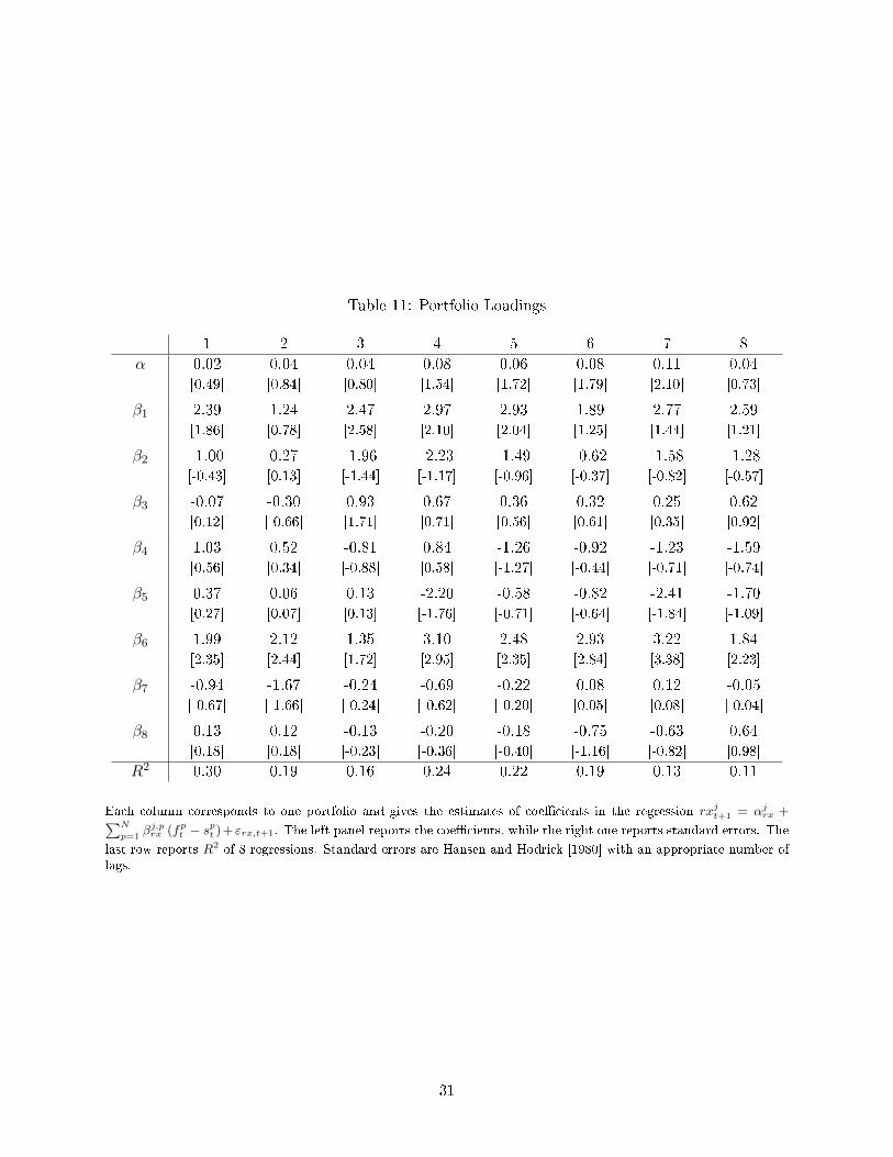
Table 11: Portfolio Loadings

1 2 3 4 5 6 7 8

α 0.02 0.04 0.04 0.08 0.06 0.08 0.11 0.04[0.49] [0.84] [0.80] [1.54] [1.72] [1.79] [2.10] [0.73]

β1 2.39 1.24 2.47 2.97 2.93 1.89 2.77 2.59[1.86] [0.78] [2.58] [2.10] [2.04] [1.25] [1.44] [1.21]

β2 -1.00 0.27 -1.96 -2.23 -1.49 -0.62 -1.58 -1.28[-0.43] [0.13] [-1.44] [-1.17] [-0.96] [-0.37] [-0.82] [-0.57]

β3 -0.07 -0.30 0.93 0.67 0.36 0.32 0.25 0.62[0.12] [-0.66] [1.71] [0.71] [0.56] [0.61] [0.35] [0.92]

β4 1.03 0.52 -0.81 0.84 -1.26 -0.92 -1.23 -1.59[0.56] [0.34] [-0.88] [0.58] [-1.27] [-0.44] [-0.71] [-0.74]

β5 0.37 0.06 0.13 -2.20 -0.58 -0.82 -2.41 -1.70[0.27] [0.07] [0.13] [-1.76] [-0.71] [-0.64] [-1.84] [-1.09]

β6 1.99 2.12 1.35 3.10 2.48 2.93 3.22 1.84[2.35] [2.44] [1.72] [2.95] [2.35] [2.84] [3.38] [2.23]

β7 -0.94 -1.67 -0.24 -0.69 -0.22 0.08 0.12 -0.05[-0.67] [-1.66] [-0.24] [-0.62] [-0.20] [0.05] [0.08] [-0.04]

β8 0.13 0.12 -0.13 -0.20 -0.18 -0.75 -0.63 0.64[0.18] [0.18] [-0.23] [-0.36] [-0.40] [-1.16] [-0.82] [0.98]

R2 0.30 0.19 0.16 0.24 0.22 0.19 0.13 0.11

Each column corresponds to one portfolio and gives the estimates of coe�cients in the regression rxjt+1 = αjrx +∑N

p=1βj,prx (fp

t − spt )+εrx,t+1. The left panel reports the coe�cients, while the right one reports standard errors. The

last row reports R2 of 8 regressions. Standard errors are Hansen and Hodrick [1980] with an appropriate number oflags.

31

Figure 12: Loadings on all forward-spot spreads and an extracted single factor

2 4 6 8

−2

0

2

Load

ings

Portfolio 1

2 4 6 8

−2

0

2Lo

adin

gsPortfolio 2

2 4 6 8

−2

0

2

Load

ings

Portfolio 3

2 4 6 8

−2

0

2

Load

ings

Portfolio 4

2 4 6 8

−2

0

2

Load

ings

Portfolio 5

2 4 6 8

−2

0

2

Load

ings

Portfolio 6

2 4 6 8

−2

0

2

Load

ings

Portfolio 7

2 4 6 8

−2

0

2

Load

ings

Portfolio 8

2 4 6 8

−2

0

2

Load

ings

All loadings

Blue solid line in each graph shows the loadings of each portfolio on 8 forward-spot spreads. Red dotted line showsan extracted single factor as the �rst principal component of all 8 loadings. The last �gure plots all loadings in asingle graph to assess single factor structure.

32

Table 12: Return predictability with AD factor

1 2 3 4 5 6 7 8

βFBrx 2.96 2.07 1.53 2.80 2.20 2.18 0.36 0.76(0.41) (0.45) (0.46) (1.13) (0.89) (0.99) (0.74) (0.35)

βADrx 3.70 2.19 1.82 2.57 2.31 2.25 1.07 1.79(0.61) (0.58) (0.61) (0.96) (0.77) (0.95) (1.07) (1.32)

R2FB 24.92 12.96 9.57 14.97 9.96 11.26 0.45 3.95

R2AD 22.33 9.83 8.69 12.34 12.78 9.98 2.27 5.47R2O 29.95 18.80 16.09 24.13 22.24 19.46 12.59 10.86

The table reports estimates, standard errors and R2 of several regressions. In the �rst one, I run the usual ft −st+1 = αrx + βFB

r (ft − st) + εrx,t regression and report the coe�cient on forward spread and R2. In the secondspeci�cation I form a single factor as a simple average of forward spreads across countries and estimate ft − st+1 =αrx + βAD

rx

∑N

p=1(i∗pt − it) + εrx,t regression. In the third speci�cation, I regress excess returns on the �rst principal

component of eigen-value decomposition of expected returns (formed by regressing excess returns on all interest ratedi�erentials and taking the �tted values). Only R2

O of this regression is reported. Standard errors are Hansen andHodrick [1980] with an appropriate number of lags.

have uninterpretable negative/positive swings and are susceptible to over�tting and multicollinearity

issues.

To test the single factor story formally, I form the single factor using eigen-value decomposition of

expected returns and compare the results with the usual forward spread regression and the regression

with a single factor formed as a simple average of forward spreads across countries. While the single

factor variable formed using the eigen-value decomposition of expected returns seems to perform

better than usual forward-spot di�erential (in terms of R2), the di�erence is not very convincing

and can easily be a result of a simple over�tting.

The average interest rate di�erential (AD) factor Instead of forming an optimal linear

combination of loadings by eigen-value decomposition, we might as well take a simple arithmetic

average of them. Such a construction is easily interpretable: it tells us how high home country's

interest rate is relative to the average interest rate in all other countries. This approach was

undertaken also in Lustig et al. [2010b]. Each country is getting the same weight. Potentially, we

may use higher weights for larger countries, i.e. perform something like GDP-weighting.

Estimates of the average interest rate di�erential and the usual country-speci�c di�erential

predictive regression are shown in Table 12. It is important that the AD factor is not worse than

portfolio speci�c di�erential on average, which suggests in favor of a single factor structure story.

Table 13 shows the estimates for ∆st+1 regression. The average forward spread factor seems to

perform about the same as simple individual forward spread regression at annual horizon.

To sum up, the average interest rate di�erential seems to perform as well as the portfolio-speci�c

one. However, we know that if ∆s were a random walk, the interest rate di�erential would be the

only true predictor of foreign exchange. This suggests in favor of the risk premium story, where

excess returns are related to marginal utility of investors rather than speci�c characteristics of assets.

33

Table 13: Comparing R2 for ∆st+1

1 2 3 4 5 6 7 8

βFB∆s -1.96 -1.07 -0.53 -1.80 -1.20 -1.18 0.64 0.24(0.41) (0.45) (0.46) (1.13) (0.89) (0.99) (0.74) (0.35)

βAD∆s -2.66 -1.18 -0.81 -1.68 -1.52 -1.26 0.00 -0.58(0.60) (0.55) (0.64) (0.96) (0.79) (0.96) (1.01) (1.21)

R2FB 12.69 3.83 1.25 6.77 3.17 3.58 1.46 0.38

R2AD 13.46 3.14 1.85 5.81 5.95 3.43 -0.01 0.59R2O 18.53 10.28 8.38 16.81 16.37 12.48 13.47 7.55

The table reports estimates, standard errors and R2 of several regressions. In the �rst one, I run the usual∆st+1 = α∆s + βFB

∆s (ft − st) + ε∆s,t regression and report the coe�cient on forward spread and R2. In thesecond speci�cation I form a single factor as a simple average of forward spreads across countries and estimate∆st+1 = α∆s + βAD

∆s

∑N

p=1(i∗pt − it) + ε∆s,t regression. In the third speci�cation, I regress excess returns on the �rst

principal component of eigen-value decomposition of expected returns (formed by regressing excess returns on allinterest rate di�erentials and taking the �tted values). Only R2

O of this regression is reported. Standard errors areHansen and Hodrick [1980] with an appropriate number of lags.

In what follows I will use the average interest rate di�erential as a universal home country-speci�c

forecasting factor of exchange rates.

The carry-trade risk factor Lustig et al. [2010a] show that the carry-trade risk factor does exist

in the cross-section of foreign exchange. The literature, however, is silent on what is the underlying

predictor of this factor in time-series, if the risk premium is time-varying.

The two factor decomposition in foreign exchange markets discussed is similar to the one for

international bond markets: I modeled the bond market risk premium by using two factors as well.

This symmetry in modeling across asset markets makes it easy to compare risk premia. The bond

market's global CP factor seems like a direct equivalent of the foreign exchange market's carry

trade factor. Country-speci�c bond and foreign exchange factors are related too. In terms of the

risk premium macro story we can expect global risk factors to be related to global business cycles

while country-speci�c factors to re�ect country-speci�c business cycle type of risk (net of global).

If this were true and the bond global risk factor were indeed related to foreign exchange carry

trade factor, it would then follow that the bond GCP factor should predict foreign exchange carry

trade returns. This is tested in Table 14.

Table 14 and Figure 13 show that carry trade returns are negatively correlated with the GCP

factor. We know that average return on carry trade is higher, but this return is lower when marginal

utility of investors is high. This has been documented in Lustig and Verdelhan [2007] and Lustig

et al. [2010a]. The result in Table 14, however, says even more: not only the contemporaneous

correlation between the GCP and foreign exchange ex-post returns on carry trade is negative, but

higher GCP today (higher expected excess returns on bonds) predicts relatively lower expected

excess returns on carry trade. Part of this predictability comes from changes in spot rates and

part � from interest di�erential component, as can be seen in Table 15. This result is quite robust:

34

Figure 13: Carry trade and global CP

89 90 91 92 93 94 94 95 96 97 98 99 00 01 02 03 04 05 06 07 08 09−0.4

−0.3

−0.2

−0.1

0

0.1

0.2

0.3

0.4

0.5

0.6

Bottom black line shows carry trade excess returns. Top red line depicts the global CP factor (scaled).

Table 14: Predicting portfolio returns with global CP and average di�erential factors

Carry 1 2 3 4 5 6 7 8

α 0.18 -0.05 -0.03 -0.00 -0.00 -0.02 0.02 0.07 0.13[2.76] [-1.06] [-0.80] [-0.09] [-0.00] [-0.48] [0.47] [1.53] [2.53]

βGCP -2.85 0.03 0.45 -0.34 -0.14 0.28 0.31 -1.10 -2.82[-1.73] [0.03] [0.46] [-0.34] [-0.13] [0.33] [0.33] [-0.92] [-1.95]

βAD -2.95 3.01 0.83 1.32 1.47 1.70 1.00 0.36 0.06[-2.03] [2.70] [0.74] [1.05] [1.14] [1.69] [0.84] [0.27] [0.04]

R2 0.18 0.23 0.02 0.05 0.04 0.07 0.02 0.02 0.08

The table reports estimates of foreign exchange excess returns of various portfolios on two factors: GCP and AD.Estimates of coe�cients, t-statistics and R2 for portfolios 1 through 8 are reported in columns numbered 1-8. The�rst column reports the estimates for carry trade strategy (8 minus 1). Standard errors are Hansen and Hodrick[1980] with an appropriate number of lags.

35

Table 15: Predicting ∆st+1 with global CP and average di�erential factors

Carry 1 2 3 4 5 6 7 8

α -0.05 0.00 0.01 -0.02 -0.02 0.01 -0.01 -0.04 -0.05[-0.83] [0.02] [0.22] [-0.42] [-0.39] [0.22] [-0.38] [-0.86] [-0.93]

βGCP 1.38 0.33 -0.27 0.57 0.45 -0.01 -0.28 0.82 1.71[0.92] [0.33] [-0.28] [0.55] [0.42] [-0.02] [-0.30] [0.70] [1.24]

βAD 3.78 -2.31 -0.17 -0.54 -0.61 -0.75 0.21 0.95 1.47[3.16] [-2.17] [-0.15] [-0.44] [-0.47] [-0.74] [0.17] [0.74] [1.01]

R2 0.22 0.17 0.00 0.01 0.01 0.01 0.00 0.03 0.07

The table reports estimates of foreign exchange spot change of various portfolios on two factors: GCP and AD.Estimates of coe�cients, t-statistics and R2 for portfolios 1 through 8 are reported in columns numbered 1-8. The�rst column reports the estimates for carry trade strategy (8 minus 1). Standard errors are Hansen and Hodrick[1980] with an appropriate number of lags.

it holds for both GDP- and equal-weighted GCP factors, as well as a GCP factor constructed by

extracting 5 principal components from all forwards.

R2 of the �rst portfolio is much higher and it may seem that carry trade results are driven by

this fact; however, the results are robust when choosing other portfolios to form carry trade. For

example, if we choose 8 minus 2, R2 of carry trade is about 15% and the coe�cients are similar.

Patterns in coe�cients of portfolio excess returns on two factors are interesting too. Slopes

on the AD factor are the highest for low interest rate countries and close to zero for high ones.

The average risk premia (α) is negative for low interest rate countries, and highly positive for high

interest rate countries. Therefore, investing in low interest rate portfolio delivers negative average

returns (as documented by Lustig et al. [2010a]), but is sensitive to the AD factor in time. The

AD factor hence predicts the time varying risk premium for low interest rate portfolios only. This

means that investing in low interest countries bears signi�cant amount of the US-speci�c time-

varying foreign exchange risk. This risk is essentially absent when investing in high interest rate

countries since the movements in US interest rates are relatively small compared to the movements

in high interest rate countries.

Time-varying risk premia of high interest rate countries are mostly driven by the carry trade

(GCP) factor. Indeed, slopes of low interest rate countries on the GCP factor are essentially zero,

while high interest rate countries have signi�cant negative slopes. This is the sense in which high

interest rate countries are riskier: they depreciate in bad times (when GCP is high) and expectedly

so. The average return on high interest rate portfolios (α) is of course signi�cantly higher than

that of low portfolios as was documented by Lustig et al. [2010a]. Carry trade α is positive and

signi�cant. It is therefore most pro�table to invest in carry when GCP is low and US interest rate

is relatively high.

We therefore have two factors that predict foreign exchange in time-series: a country speci�c

and a global one. First one is the usual one � high expected returns when marginal utility is high

36

and people want to consume today. The second one re�ects the risk associated with involving in

risky carry trade strategies: while the returns on these strategies are higher on average, the carry

trade factor makes higher interest rate countries more risky and prone to devaluations, especially

when the economy is doing poorly. Carry trade is a global factor. By focusing on high/low interest

rate sorted portfolios, we are able to isolate common innovations to the stochastic discount factor

(SDF) as was emphasized by Lustig et al. [2010a].

4 The Model

4.1 Long-run risk model

The use of two factors outlined in the paper can be motivated by a long-run risk model similar to

the one in Bansal and Shaliastovich [2009] and Bansal and Yaron [2004]. The model of this type has

been shown (see Bansal et al. [2006]) to be potent in explaining asset returns. In addition, Colacito

et al. [2010] argued that long-run risk model can also explain a wide range of international �nance

puzzles, including the high correlation of international stock markets, despite the lack of correlation

in fundamentals.

In what follows I provide a speci�cation of the model that motivates the empirical section of the

paper. The model, however, is neither estimated nor formally tested in this paper. For empirical

support see Bansal et al. [2006], Bansal and Shaliastovich [2009] and Section 4.2.

4.1.1 Consumption Process

Let the consumption dynamics in home country be governed by

∆ct+1 = µg + xt + σgtηt+1 (2)

xt+1 = ρxt + σxtet+1 (3)

σ2g,t+1 = νgσ

2gt + wg,t+1 (4)

σ2x,t+1 = νxσ

2xt + wx,t+1 (5)

Consumption contains a predictable component xt. Both the variance of predictable and id-

iosyncratic components are heteroskedastic. I assume that the consumption and expected growth

innovations ηt+1 and et+1 are standard Normal, while the innovations to volatility processes wg,t+1

and wx,t+1 follow Gamma distribution Γ(σ2i (1− νi), σ2

iw), i = {g, x}.

4.1.2 Discount Factor

Bansal and Shaliastovich [2009] show that in this speci�cation with Epstein and Zin [1989] prefer-

ences, discount factor takes the form

mt+1 = θlogδ − θ

ψ∆ct+1 + (θ − 1) rc,t+1 (6)

37

where the return on consumption rc,t+1 is given by

rc,t+1 = κ0 + κ1pct+1 − pct + ∆ct+1

and price-consumption ratio pct can be shown to be linear in states,

pct = A0 +Axxt +Agsσ2gt +Axsσ

2xt

Substituting these into (6) gives

mt+1 = m0 +mxxt +mgsσ2gt +mxsσ

2xt − λησgtηt+1 (7)

−λeσxtet+1 − λgwwg,t+1 − λxwwx,t+1

where

mx =1

ψ

mgs = −1

2

(γ − 1

ψ

)(γ − 1)

mxs = −1

2

(γ − 1

ψ

)(γ − 1)

(κ1

1− κ1ρ

)2

4.1.3 Real Yields and Bond Risk Premia

Now we can derive expressions for real yields and real bond risk premia,

y(n)t =

1

n

(B

(n)0 +B(n)

x xt +B(n)gs σ

2gt +B(n)

xs σ2xt

)Real bond risk premia is (see Section 6.6.1 for derivation):

Et(rx

(n)t+1

)= const+

(B(n)xs − νxB(n−1)

xs −B(1)xs −

1

2λ2e

)× σ2

xt

4.1.4 Foreign Country

Consider a foreign country. Assume that the variances of persistent component are proportional

∆c∗t+1 = µg + x∗t + σ∗gtη∗t+1

x∗t+1 = ρx∗t + λ∗σxtet+1

σ∗2g,t+1 = νgσ∗2gt + w∗g,t+1

σ2x,t+1 = νxσ

2xt + wx,t+1

38

Interest rate di�erential is

y(1)t − y

∗(1)t = B(1)

x (1− λ)xt +B(1)gs

(σ2gt − σ∗2gt

)+(1− λ∗2

)B(1)xs σ

2xt (8)

Stars (∗) denote country-speci�c variables. Thus I assume that innovations to short-term con-

sumption growth and its variance are i.i.d. across countries, while the innovations to long-term

consumption component and corresponding variance are perfectly correlated across countries. Ex-

pected consumption growth x∗t+1 of a foreign country loads proportionally on this common inno-

vation, which ultimately makes all xt's proportional across countries. This assumption re�ects the

desire to make SDFs highly correlated across countries � the condition that must be satis�ed ac-

cording to Brandt et al. [2006]. The motivation to make only long-run components correlated comes

from the view that developed countries have similar expected long-run consumption growth rates

(are cointegrated).

4.1.5 In�ation Process

I specify in�ation process exogenously as in Bansal and Shaliastovich [2009]. In�ation is a�ected

by real economy, but does not feed back to it.

Let the in�ation process be

πt+1 = µπ + zt + ϕπgσgtηt+1 + ϕπxσxtet+1 + σπξt+1

where zt is the expected in�ation that in turn follows

zt+1 = αzzt + αxxt + ϕzgσgtηt+1 + ϕzxσxtet+1 + σzξz,t+1

I further assume that in�ation and expected in�ation do not respond to short-term news, ϕπg =

ϕzg = 0.

4.1.6 Nominal Yields and Bond Risk Premia

In what follows all nominal variables will be denoted with a dollar ($) sign.

Nominal discount factor Nominal discount factor is

m$t+1 = mt+1 − πt+1

m$t+1 = (m0 − µπ) +mxxt − zt +mgsσ

2gt +mxsσ

2xt − (λη + ϕπg)σgtηt+1

− (λe + ϕπx)σxtet+1 − λgwwg,t+1 − λxwwx,t+1 − σπξt+1

Nominal bond yields

39

y(n)t,$ =

1

n

(B

(n)0,$ +B

(n)x,$xt +B

(n)gs,$σ

2gt +B

(n)xs,$σ

2xt +B

(n)z,$ zt

)

Nominal bond risk premia Expected log nominal bond risk premia is (see Section 6.6.2 for

derivation):

Et(rx

(n)t+1,$

)= const+

(B

(n)xs,$ − νxB

(n−1)xs,$ −B(1)

xs,$

)σ2xt (9)

Time varying part of the nominal bond risk premium depends on variance of long-run component

only. This motivates using a common component of CP factors to predict foreign exchange risk

premia. If all countries have the same σ2xt or they share a common component, we can use CPs

as an estimate of conditional variance of long-run consumption component xt (assuming that CP

factors is a good proxy for bond risk premium). xt is strongly correlated across countries and is a

global factor.

Lustig et al. [2010a] show that countries load di�erentially on the global factor. Under the

assumption that the loadings on the shock in (3) are proportional across countries, parameter λ∗ in

the speci�cation of the model re�ects exactly this di�erential loading on a global factor (I assume

that the loading is constant in time).

Interest rate di�erential

y(1)t − y

∗(1)t = B

(1)x,$ (1− λ)xt +B

(1)gs,$

(σ2gt − σ∗2gt

)+(1− λ∗2

)B

(1)xs,$σ

2xt +B

(n)z,$ (zt − z∗t )

We can now average the interest rate di�erential across (developed) countries. Under the as-

sumption that all foreign λ's sum up to unity, the �rst term drops out. Furthermore, if the US

in�ation is highly correlated with the average in�ation in developed countries, we might expect the

last term to be of a second order importance (this should be checked empirically!). In this case the

average interest rate di�erential (AD factor in my empirical part) is a function on two conditional

variances only.

Currency excess returns Plug this into FX excess returns:

Et(rxFX,$t+1

)= Et

(st+1 − st + y

∗(1)t − y(1)

t

)= Et[−

(m0 +mxxt − zt +mgsσ

2gt +mxsσ

2xt − εt+1

)+(m0 +mxx

∗t − z∗t +mgsσ

∗2gt +mxsλ

2σ2xt − ε∗t+1

)+ y∗(1)t − y(1)

t ]

= −(mgs −mgs −

1

2γ2)(

σ2gt − σ∗2gt

)−(mxs +B(1)

xs

) (1− λ2

)σ2xt

=1

2γ2(σ2gt − σ∗2gt

)+

1

2λ2eσ

2xt

40

Foreign exchange risk premium is therefore a linear function of the variance of long-term consump-

tion component and the di�erence between short-term variances between two countries. If we invest

in a well diversi�ed portfolio of currencies, the latter term becomes the variance of a home country

short-term consumption growth.

4.1.7 Two Factors

Given the functional forms above, the risk premia on a diversi�ed portfolio of currencies can be

recovered from two state variables: σ2xt and σ

2gt. The �rst one can be proxied by the average CP

factor across developed countries (GCP factors in the empirical part), while the second one can

be estimated by a linear combination of GCP factor and the average interest rate di�erential (AD

factor in the empirical part). In other words, we should be able to �nd expected excess returns on

a portfolio of currencies by regressing the foreign exchange risk premia on AD and GCP factors.

4.2 Empirical Support

4.2.1 Estimating Consumption Volatility

Equation (9) says that the time variation in expected excess bond returns is driven by a single factor

- conditional variance of an expected consumption growth. If we believe that expected excess bond

return is reasonably well proxied by the Cochrane-Piazzesi factor, this implies that CP factor and

σ2xt are closely linked. While this is a theoretical outcome of my model speci�cation, it might seem

not overly convincing. To explore the relationship between the two, I construct an estimate of σ2xt

using consumption data and compare it to the CP factor.

In constructing the estimate of σ2xt I follow a similar approach to Bansal et al. [2006]. In

particular I estimate the volatility of predictable consumption component as follows:

1. Use monthly consumption growth data; work at annual horizon

2. Regress log consumption growth on a set of predictors (dividend growth, DP, risk free rate,

return on market portfolio, lag of consumption growth)

3. Use the predicted part in place of xt

4. Perform AR(1) regression of xt on xt−1

5. Square the residual and regress on a set of predictors in 2 + lagged residual^2

6. Square the residual of regression in 4 is shown on the �rst plot below; predicted part is shown

on the second plot

Plot 14 shows the estimates of σ2xt. I also present it side-by-side with the CP factor plot. There

are some similarities... Correlation is ~20%. Notice hat both estimation techniques are rather ad

hoc and quite noisy, so we cannot expect a perfect correlation here. Remember also that CP factors

41

Figure 14: Volatility of predictable consumption component and CP factor

.0000

.0001

.0002

.0003

.0004

.0005

.0006

.0007

60 65 70 75 80 85 90 95 00 05 10

DCFU2

-.00001

.00000

.00001

.00002

.00003

.00004

.00005

.00006

65 70 75 80 85 90 95 00 05

CPX DCFU2F

-.00002

.00000

.00002

.00004

.00006

.00008

.00010

.00012

60 65 70 75 80 85 90 95 00 05 10

DCFU2F 1955 1960 1965 1970 1975 1980 1985 1990 1995 2000 2005

−0.04

−0.02

0

0.02

0.04

0.06

0.08

0.1

0.12

0.14

The �rst plot shows the conditional variance of expected consumption growth. The bottom left plotshows estimated value of σ2

xt; the last plot shows the CP factor. The top-right plot combines thetwo (rescaled).

42

were far from perfectly correlated across countries (although xt's are perfectly correlated in the

model). All in all, there is some plausibility in this story, but it should be further investigated.

TO BE COMPLETED

5 Conclusions

I have documented new empirical �ndings for bond and foreign exchange markets. For bond market,

I have shown that CP factors similar to the US one can also be documented in other countries.

Further, I showed that those CP factors are correlated and a common component can be extracted.

This common component can be interpreted as a global bond factor, which, together with the

country speci�c CP-factor, can explain bond returns in the the cross-section of countries.

I found a similar two factor structure in the foreign exchange market. The AD factor is related

to the country-speci�c CP factors and the foreign exchange global factor is related to the GCP

factor. In fact, the GCP factor helps to predict foreign exchange returns. The GCP and AD factors

are both signi�cant in predicting foreign exchange returns and vary in their importance with the

riskiness of a country (as measured by forward spread).

The �ndings in the paper provide evidence in favor of the risk premia story. I show that risk

premia in both markets are strongly linked and should be studied jointly. An interesting extension

of this paper would be to construct an SDF model where time-varying risk premia in bond and

foreign exchange markets are governed by the factors I have documented. The easiest approach

to do this is by extending the Cochrane and Piazzesi [2009] and Koijen et al. [2010] models to an

international setting. I provide my initial thoughts on implementing this exercise in the appendix.

Additionally, pricing the stock market is interesting as well. Ultimately, we would like to link the

risk premia in all three markets together.

The paper points out to several additional areas that are under-researched and might be a

useful continuation of the current work. First, I have shown that the data reported by Central

Banks and other sources are typically smoothed across maturities and this smoothing destroys useful

information. Fama and Bliss [1987] data, on the other hand, seem to preserve the information that

is eliminated by smoothing procedures. It is therefore interesting to construct alternative discount

bonds series for foreign countries that use approach similar to that of Fama and Bliss [1987]. Fama

and Bliss [1987] results themselves could be extended to longer maturities. Additionally, there is

some evidence that their approach does not work well in the recent crisis, when the prices of on-the-

run and o�-the-run bonds di�ered substantially. It would then be useful to update their approach

to account for this issue. This extension is an ongoing project.

Second, I suggested a way to test whether including additional forward rates in estimating the

CP factor is useful. To accomplish this, I propose to specify the null in the form of a discount factor

model that imposes that CP factor is fully explained by the �rst �ve forward rates. Under this null,

additional forward rates should be irrelevant and by including them we can construct bounds on

the distribution of R2 of bond predictive regressions. This test di�ers from a simple χ2 test and is

43

more powerful.

Third, given the predictability and correlations between markets documented, it would be inter-

esting to test the performance of actual trading strategies that combine bond and foreign exchange

investments. Since carry trade risk premia was found to be negatively correlated with GCP factor,

investing in two markets simultaneously may partially hedge the risks. It would then be interesting

to document the Sharpe ratios and performance of such investment strategies.

44

6 Appendix

6.1 A�ne model

6.1.1 Setup

In discrete time specify the dynamics of state variables as

Xt+1 = µ+ φXt + vt+1, E(vt+1v

′t+1

)= V

Let a discount factor be governed by

Mt+1 = exp

(−δ0 − δ

′1Xt −

1

2λ′tV λt − λ

′tvt+1

)λt = λ0 + λ1Xt

6.1.2 Bond prices

Zero-coupon bond prices can be shown to be linear functions of factors:

p(n)t = logEt

(n∏i=1

Mt+i

)= An +B

′nXt

Coe�cients An, Bn are given by recursion:

A0 = 0; B0 = 0

B′n+1 = −δ′1 +B

′nφ∗

An+1 = −δ0 +An +B′nµ∗ +

1

2B′nV Bn

where φ∗, µ∗ are de�ned as

φ∗ = φ− V λ1

µ∗ = µ− V λ0

For the proof see Cochrane and Piazzesi [2005], Appendix D.1.

Yields are given by

y(n)t = −An

n− B

′n

nXt

45

Forward rates are

f(n)t = p

(n−1)t − p(n)

t

= (An−1 −An) +(B′n−1 −Bn

)Xt

= Afn +Bf ′n Xt

6.1.3 Bond excess return

Bond excess return is

rx(n)t+1 = p

(n−1)t+1 − p(n)

t + p(1)t

= An−1 +B′n−1 (µ+ φXt + vt+1)

−(An +B

′nXt

)−(A0 +B

′0Xt

)

Et(rx

(n)t+1

)+

1

2σt(rx

(n)t+1

)= covt (rxt+1, vt+1)λt

= B′n−1V (λ0 + λ1Xt)

= B′n−1 (µ− µ∗) +B

′n−1 (φ− φ∗)Xt

6.2 Foreign exchange risk premium in a�ne model

Following Backus et al. [2001], consider pricing excess return:

Et [Mt+1 (Ft − St+1)] = 0

Dividing through by St and taking logs yields:

ft − st = logEtM∗t+1 − logEtMt+1

Recall the decomposition

ft − st = [Etst+1 − st] + [ft − Etst+1]

= qt + pt

When markets are complete, the following identity links SDFs and exchange rates

logM∗t+1 − logMt+1 = st+1 − st

46

It then immediately follows that

qt = Etst+1 − st = EtlogM∗t+1 − EtlogMt+1

= − (δ∗0 − δ0)−(δ∗′

1 X∗t − δ

′1Xt

)− 1

2

(λ∗′t V∗λ∗t − λ

′tV λt

)Then the risk premium is given by

pt =(logEtM

∗t+1 − logEtMt+1

)−(EtlogM

∗t+1 − EtlogMt+1

)=

1

2

(λ∗′t V∗λ∗t − λ

′tV λt

)Expected appreciation is quadratic in factors.

This is an extension of expectation hypothesis. We do need λt vary over time to generate

time-varying risk premium.

6.3 Single CP speci�cation

6.3.1 Time-varying risk premium

Suppose Xt contains only country-speci�c yield curve factors. Cochrane and Piazzesi [2009]show

that the process for λt can be restricted as follows

λt =

0

λ0l

0

0

+

0 0 0 0

λ1l 0 0 0

0 0 0 0

0 0 0 0

xt

levelt

slopet

curvet

6.3.2 Implied foreign exchange risk premia

λ′tV λt = λ

′0V λ0 + λ

′0V λ1Xt +X

′tλ′1V λ0 +X

′tλ′1V λ1Xt

= v22λ20l + 2λ0lv22λ1lxt + λ2

1lv22x2t

Therefore foreign exchange risk premium is

pt =1

2

(λ∗′t V∗λ∗t − λ

′tV λt

)=

1

2

(v∗22λ

∗20l − v22λ

20l

)+ (λ∗0lv

∗22λ∗1lx∗t − λ0lv22λ1lxt)

+1

2

(v∗22λ

∗21l x∗2t − v22λ

21lx

2t

)

47

6.4 GCP and country-speci�c CP speci�cation

6.4.1 Time-varying risk premium

Suppose Xt contains only country-speci�c yield curve factors. Cochrane and Piazzesi [2009]show

that the process for λt can be restricted as follows

λt =

0

0

λ0l

0

0

+

0 0 0 0 0

0 0 0 0 0

λCP1l λGCP1l 0 0 0

0 0 0 0 0

0 0 0 0 0

xCPt

xGCPt

levelt

slopet

curvet

Market price of risk depend only on CP and GCP and are earned in compensation to exposure

to level shock only, as documented by Cochrane and Piazzesi [2009].

6.4.2 Implied foreign exchange risk premia

λ′tV λt = λ

′0V λ0 + λ

′0V λ1Xt +X

′tλ′1V λ0 +X

′tλ′1V λ1Xt

= v33λ20l + 2λ0lv33

(λCP1l x

CPt + λGCP1l xGCPt

)+v33

(xCPt λCP1l + xGCPt λGCP1l

)2

Therefore foreign exchange risk premium is

pt =1

2

(λ∗′t V∗λ∗t − λ

′tV λt

)=

1

2

(v∗33λ

∗20l − v33λ

20l

)+[λ∗0lv

∗33

(λ∗CP1l x∗CPt + λ∗GCP1l xGCPt

)− λ0lv33

(λCP1l x

CPt + λGCP1l xGCPt

)]+

1

2

[v∗33

(x∗CPt λ∗CP1l + xGCPt λ∗GCP1l

)2− v33

(xCPt λCP1l + xGCPt λGCP1l

)2]

6.5 Two factor model example

Lustig et al. [2010b] show that if an SDF for country i is speci�ed as −mit+1 = λzit +

√γzitu

it+1 +

τzwt +√δizwt u

wt+1, where z

it and zwt are components of the state vector X that correspond to a

country-speci�c factor (zit) and common factor (zwt ), the risk premium corrected for the Jensen

term is

Et[rxit+1

]+

1

2V ar

(rxit+1

)= γzt −

√δizwt

√δzwt + δizwt

48

=√δi(√

δ −√δi)zwt + γzt (10)

Lustig et al. [2010b] further argue that this expression does not depend on country-speci�c factor

zit and hence this calculation can be used as a motivation towards looking for a �common factor� in

the foreign exchange market.

6.6 Long-Run Risk Model

6.6.1 Real Bond Risk Premia

rx(n)t+1 =

(p

(n−1)t+1 − p(n)

t

)− y(1)

t = ny(n)t − (n− 1) y

(n−1)t+1 − y(1)

t

= B(n)0 +B(n)

x xt +B(n)gs σ

2gt +B(n)

xs σ2xt

−(B

(n−1)0 +B(n−1)

x xt+1 +B(n−1)gs σ2

g,t+1 +B(n−1)xs σ2

x,t+1

)− y(1)

t

=(B

(n)0 −B(n−1)

0 −B(1)0

)+(B(n)x − ρB(n−1)

x −B(1)x

)xt +

(B(n)gs − νgB(n−1)

gs −B(1)gs

)σ2gt

+(B(n)xs − νxB(n−1)

xs −B(1)xs

)σ2xt −B(n−1)

x σxtet+1 −B(n−1)gs wg,t+1 −B(n−1)

xs wx,t+1

0 =(B(n)gs − νgB(n−1)

gs −B(1)gs

)where the constants are given by recursion:

B(n)x = ρB(n−1)

x −mx

B(n)gs = νgB

(n−1)gs −mgs −

1

2γ2

B(n)xs = νxB

(n−1)xs −mxs −

1

2

(λe +B(n−1)

x

)2

Expected excess returns are then

Et(rx

(n)t+1

)+

1

2vart

(rx

(n)t+1

)= −covt (mt+1, rxt+1,n)

= const+ c× σ2xt

vart(rx

(n)t+1

)= λ2

eσ2xt + const

6.6.2 Nominal Bond Risk Premia

Nominal bond excess return is given by:

49

rx(n)t+1,$ =

(p

(n−1)t+1,$ − p

(n)t,$

)− y(1)

t,$ = ny(n)t,$ − (n− 1) y

(n−1)t+1,$ − y

(1)t,$

= B(n)0,$ +B

(n)x,$xt +B

(n)gs,$σ

2gt,$ +B

(n)xs,$σ

2xt +B

(n)z,$ zt

−(B

(n−1)0,$ +B

(n−1)x,$ xt+1 +B

(n−1)gs,$ σ2

g,t+1 +B(n−1)xs,$ σ2

x,t+1 +B(n−1)z,$ zt+1

)− y(1)

t

=(B

(n)0,$ −B

(n−1)0,$ −B(1)

0,$

)+(B

(n)x,$ − ρB

(n−1)x,$ −B(1)

x,$ −B(n−1)z,$ αx

)xt +

(B

(n)z,$ − αzB

(n−1)z,$ −B(1)

z,$

)zt +

(B

(n)gs,$ − νgB

(n−1)gs,$ −B(1)

gs,$

)σ2gt

+(B

(n)xs,$ − νxB

(n−1)xs,$ −B(1)

xs,$

)σ2xt −

(B

(n−1)x,$ +B

(n−1)z,$ ϕzx

)σxtet+1 −B(n−1)

gs,$ wg,t+1 −B(n−1)xs,$ wx,t+1 −B(n−1)

z,$ ϕzgσgtηt+1 −B(n−1)z,$ σzξz,t+1

where the constants are given by recursion:

B(n)x,$ = ρB

(n−1)x,$ −mx − αxB(n−1)

z,$

B(n)z,$ = αzB

(n−1)z,$ + 1

B(n)gs,$ = νgB

(n−1)gs,$ −mgs −

1

2(ϕπg + γ + ϕzgB

(n−1)z,$ )2

B(n)xs,$ = νxB

(n−1)xs,$ −mxs −

1

2

(ϕπx + λe +B

(n−1)x,$ + ϕzgB

(n−1)z,$

)2

Substituting these into the formula for excess returns (and assuming ϕπg = ϕzg = 0) yields

rx(n)t+1,$ = const+

(B

(n)xs,$ − νxB

(n−1)xs,$ −B(1)

xs,$

)σ2xt −

−(B

(n−1)x,$ +B

(n−1)z,$ ϕzx

)σxtet+1 −B(n−1)

gs,$ wg,t+1 −B(n−1)xs,$ wx,t+1 −B(n−1)

z,$ ϕzgσgtηt+1 −B(n−1)z,$ σzξz,t+1

50

References

A. Alexius. Uncovered interest parity revisited. Review of International Economics, 9(3):505�517,

2001.

N. Anderson and J. Sleath. New estimates of the UK real and nominal yield curves. Working paper

series - Bank of England, 2001.

A. Ang and J. Chen. Yield Curve Predictors of Foreign Exchange Returns. 2010.

D.K. Backus, S. Foresi, and C.I. Telmer. A�ne term structure models and the forward premium

anomaly. Journal of Finance, 56(1):279�304, 2001.

R. Bansal and I. Shaliastovich. A long-run risks explanation of predictability puzzles in bond and

currency markets. Manuscript, Duke University, 2009.

R. Bansal and A. Yaron. Risks for the long run: A potential resolution of asset pricing puzzles. The

Journal of Finance, 59(4):1481�1509, 2004.

R. Bansal, D. Kiku, and A. Yaron. Risks for the long run: Estimation and inference. Manuscript,

Department of Economics, Duke University, Durham NC, 2006.

M.W. Brandt, J.H. Cochrane, and P. Santa-Clara. International risk sharing is better than you

think, or exchange rates are too smooth. Journal of Monetary Economics, 53(4):671�698, 2006.

Deutsche Bundesbank. Estimating the term structure of interest rates. Deutsche Bundesbank

Monthly Report. 1997.

M.D. Chinn and G. Meredith. Monetary Policy and Long-Horizon Uncovered Interest Parity. IMF

Sta� Papers, 51(3):409�431, 2004.

J.H. Cochrane. The dog that did not bark: A defense of return predictability. Review of Financial

Studies, 21(4):1533, 2008.

J.H. Cochrane and M. Piazzesi. Bond risk premia. American Economic Review, pages 138�160,

2005.

J.H. Cochrane and M. Piazzesi. Decomposing the yield curve. 2009.

R. Colacito, M.M. Croce, and U.N.C.C. Hill. Risks for the long-run and the real exchange rate.

2010.

M. Dahlquist and H. Hasseltoft. International Bond Risk Premia. 2010.

F.X. Diebold and C. Li. Forecasting the term structure of government bond yields. Journal of

Econometrics, 130(2):337�364, 2006.

51

F.X. Diebold, C. Li, and V. Yue. Global Yield Curve Dynamics and Interactions: A Generalized

Nelson-Siegel Approach. Journal of Econometrics, forthcoming, 2007.

J. Driessen, B. Melenberg, and T. Nijman. Common factors in international bond returns. Journal

of International Money and Finance, 22(5):629�656, 2003.

D. Du�e and K.J. Singleton. An econometric model of the term structure of interest-rate swap

yields. Journal of �nance, 52(4):1287�1321, 1997.

L.G. Epstein and S.E. Zin. Substitution, risk aversion, and the temporal behavior of consumption

and asset returns: A theoretical framework. Econometrica: Journal of the Econometric Society,

57(4):937�969, 1989.

E.F. Fama. Forward and spot exchange rates. Journal of Monetary Economics, 14(3):319�338,

1984.

E.F. Fama and R.R. Bliss. The information in long-maturity forward rates. The American Economic

Review, pages 680�692, 1987.

E.F. Fama and K.R. French. The cross-section of expected stock returns. Journal of �nance, 47(2):

427�465, 1992.

F. Fehle. The components of interest rate swap spreads: Theory and international evidence. Journal

of Futures Markets, 23(4):347�387, 2003.

R.S. Gürkaynak, B. Sack, and J.H. Wright. The US Treasury yield curve: 1961 to the present.

Journal of Monetary Economics, 54(8):2291�2304, 2007.

L.P. Hansen and R.J. Hodrick. Forward exchange rates as optimal predictors of future spot rates:

An econometric analysis. The Journal of Political Economy, 88(5), 1980.

S. Kessler and B. Scherer. Varying risk premia in international bond markets. Journal of Banking

& Finance, 33(8):1361�1375, 2009.

R.S.J. Koijen, H.N. Lustig, and S. Van Nieuwerburgh. The cross-section and time-series of stock

and bond returns. NBER Working Paper, 2010.

M.A. Kose, C. Otrok, and C.H. Whiteman. International business cycles: World, region, and

country-speci�c factors. American Economic Review, 93(4):1216�1239, 2003.

H. Lustig and A. Verdelhan. The cross section of foreign currency risk premia and consumption

growth risk. The American economic review, 97(1):89�117, 2007.

H. Lustig, N. Roussanov, and A. Verdelhan. Common Risk Factors in Currency Markets. 2010a.

H.N. Lustig, N.L. Roussanov, and A. Verdelhan. Countercyclical Currency Risk Premia. NBER

Working Paper, 2010b.

52

C.R. Nelson and A.F. Siegel. Parsimonious modeling of yield curves. Journal of Business, pages

473�489, 1987.

W.K. Newey and K.D. West. A simple, positive semi-de�nite, heteroskedasticity and autocorrelation

consistent covariance matrix. Econometrica: Journal of the Econometric Society, 55(3):703�708,

1987.

L.E.O. Svensson. Estimating and interpreting forward interest rates: Sweden 1992-1994. NBER

Working paper, 1994.

53