Pricing Bonds

price = PV(coupon payments) + PV(principal)

Where r = Yield to MaturityT = Time to Maturity

Tt rParValue

rCoupon

)1()1( Price

T

1t ++

+=∑

=

Yield to maturity vs. Current YieldYTM evolves from the bond price equation – Builds in the capital gain/loss from the difference

between market price and par valueCurrent Yield is just annual coupon payment divided by bond price

Interest Rate Risk

Bond prices are sensitive to interest rate changes– How?Sensitivity depends on:

1. Increase/decrease in YTM (increase less sensitive)2. Term of bond (short-term less sensitive)3. Coupon rate (higher coupons less sensitive)4. YTM (higher YTM less sensitive)

Duration

Weight the cash flows of the bond by the time when they are made– Quantifies the sensitivity of bond prices to interest rate

changes

∑=

+×=

T

t

tt

icey

CF

tD1 Pr

)1(

Duration

1. =T for zero-coupon bond2. Duration is higher for:

• Lower coupon bonds• Longer time to maturity (generally)• Lower YTM

3. =(1+y)/y for perpetuity

Passive Bond Management

Immunization– Matching durations of assets and liabilities such

that price risk and reinvestment risk exactly cancel out

Passive we’re not trying to identify undervalued securitiesStill have to monitor and actively update the portfolio– Why?

Convexity

Duration only approximates the changes in bond prices with changes in interest rates– Actual relation is not linear, but convex

Bonds generally gain more when rates fall than they lose when rates rise– Good news for bondholders– Means that more convex bonds either

»cost more and/or»have lower yields!

Active Bond Management

Usually takes the form of swaps– Substitution Swaps (based on mispricing)– Intermarket Spread Swaps (play on the yield spread)– Rate Anticipation Swaps (speculate on interest rates)– Pure Yield Pickup Swaps (move to longer duration

bonds that typically have higher rates)More on swaps in FINC416 (Spring ’07)

Chapters 11-12

Macroeconomic/Industry Analysis

Equity Valuation

Outline

Macroeconomic/Industry Analysis (Chapter 11)relies on relative valuation

Firm Specific Analysis—Equity Valuation (Chapter 12)– Dividend Discount Model– DDM and Growth Opportunities– Multistage DDM– Sensitivity Analysis– Price/Earnings Analysis

Industry AnalysisThe Business Cycle -– Trough: Economic recovery begins.

» Cyclical industries that are sensitive to the economy should do well (autos, washing machines, etc).

» High beta stocks– Peak: Entering recession.

» Defensive industries that are not sensitive to economic conditions should do well (food producers, tobacco companies, public utilities, pharmaceutical companies).

» Lower beta stocks

Sensitivity to the Business cycle depends on:(1) sales(2) operating leverage(3) financial leverage

Industry/Firm Life Cycle

Age

Sales

Start Up

Stable Growth

Consolidation

Maturity Relative Decline

Rapid and Increasing Growth

Slowing Growth

Minimal or Negative Growth

Industry/Firm Life CycleStart Up - New technology, high risk, high growth.Consolidation - Survivors are more stable, market share is more predictable, still grow faster than the overall economy.Maturity - Product reaches full potential, growth tracks growth in economy, price competition.Cash Cows - stable cash flows but little opportunity for expansion.Decline - Slow or no growth, competition or obsolete product.

Firm-Specific analysis -How do we choose stocks within an industry?

Equity Value Definitions:– Book Value - The net worth from the balance sheet– Liquidation Value - The value of the firm if broken

up and sold off (after paying off all obligations). This may provide a floor for the stock price.

– Replacement Cost - Cost to replace all assets less the value of liabilities.

Tobin’s Q = Market Price / Replacement Cost

Firm Specific AnalysisIn order to determine the value of a company, we must move away from the balance sheet and actually forecast cash flows. From forecasts, we can use models such as the Dividend Discount Model or Price to Earnings multiples to estimate firm value.

Comparing our estimate of value to the current market price tells us whether we should invest in the security.

Market Value - The price at which a security is currently trading.Intrinsic Value - The present value of expected future cash flows. This represents the value of the firm as an ongoing concern.

Intrinsic ValueWe can calculate the intrinsic value of the stock as the present value of all cash payments (including dividends and end of period sales price)

For one period:

How can we determine k?

The market’s consensus of k is the marketcapitalization rate or required rate of return.

V01 1

1=

++

E D E Pk

( ) ( )

ExampleConsider a security currently trading at $48. The security is expected to pay dividends of $3 and is expected to trade for $52 at the end of the year.If the security has a beta of 1.2, Rf=6% and the market risk premium equals 5%, what is your required rate of return for this security?

– Use the CAPM!

E(R)= 6% + 1.2 ( 5%) = 12%

Example (cont.)

Calculate the intrinsic value of the stock.

Should you buy or sell this stock?

What is your expected HPR?

Is this consistent with your buy/sell decision above?

11.49$12.1523

1)()( 11

0 =+

=++

=k

PEDEV

%58.1448

48523])([)(E(HPR) 0

011 =−+

=−+

=P

PPEDE

Example—Dividend Discount ModelConsider a firm that has a beta of 1.2 and is expected to pay dividends of $2 next year.

If the risk free rate is 4% and the market risk premium is 5%, what is the required rate of return of this stock?

Use the CAPM!E(R)= 4% + 1.2 ( 5%) = 10%

If the firm’s dividends are expected to grow at a steady rate of 6%, what is the intrinsic value of the firms shares?– Use the Value of a growing perpetuity!– V0 = D1/(r –g) = $2/(.10 - .06) = $50 per share

Cash Flow Valuations—A ReviewValue of a Perpetuity:

Value of a Constant Growth Perpetuity:

Alternatively,

– Where g is the annual growth rate in the dividend stream– k is the market capitalization rate

gPDk +=

0

1

kDV 1

0 =

gkDV−

= 10

Valuation and Stock PricingStocks represent claims on cash flows from the firm in perpetuity.– Apply the perpetuity models for stock valuation.– Stock price (Value) is represented by constant growth

dividend discount modelMore complicated analysis can incorporate the life cycle of the firm and do multiple stages of growth in the dividend discount model setting.– Used extensively by financial analysts– Aided by the use of spreadsheet modeling

Growth Opportunities (Estimating g)Earnings retention ratio (b) is the proportion of earnings not paid out in dividends but instead reinvested in the firm.

A firm that has good investment (growth) opportunities should reinvest earnings in the firm rather than paying out dividends.

If investors can reinvest the funds more profitably than the firm, earnings should be paid out in the form of dividends.

In this case: g = ROE * b

ExampleConsider three firms that have the same required rate of return (k) of 10% and are all expected to have earnings of $5 next year. ROE1 = 10%, ROE2 = 15%, ROE3 = 7.5%.

Which firms should reinvest earnings?Calculate the intrinsic value of each firm if b=0, b=0.30, b=0.60, b=0.90

What is the present value of growth opportunities (PVGO) in each case?

Note: P E

kPVGO0

1= +

No growth value Growth component

Extensions - Multistage DDMCompany ABC paid dividends this year of $4. The required rate of return for the company is 14%. You forecast dividend growth of 20% for the next four years after which growth will drop to the steady rate of 10%. What is the value per share of ABC stock?2 stages of growth:

What should you do if the stock is currently trading at $140?

443322 14.1/)2.1(414.1/)2.1(414.1/)2.1(414.1/)2.1(4 +++

27.153$)14.1/()]10.14/(.)1.1()2.1(4[ 44 =−

Sensitivity AnalysisEstimates of value will be sensitive to your forecasts of the input variables. Consider the previous example in which the value of ABC stock was estimated to be $153.27What happens to the calculated price estimate if you change yourestimate long-term growth from 10% to 9%?– Price ↓

What happens to the calculated price if you change your estimate of kfrom 14% to 13%?– Price ↑

What happens to the calculated price if you change your estimate of short-term growth from 20% to 18%?– Price ↓

How do each of these changes affect your conclusions regarding the buy/sell decision?

Price to Earnings (P/E) AnalysisWe can also obtain a price estimate by multiplying projected earnings by a forecast of the price/earnings multiple (P/E).

Consider two firms from the previous example where earnings retention ratio differed:– The firm with good growth opportunities (and b=.6) was worth

P=$200, or P/E = 200/5= 40.– The firm with no growth opportunities was worth P=$50, or

P/E = 50/5 = 10.

The Result: P/E multiples can be good indicators of growth opportunities.– Intuitively, prices reflect future expectations about cash flows.

Growth opportunities are valuable and reflected in prices (P).

P/E Analysis

The relation between P/E ratios and growth opportunities can be expressed as follows:

or

We could also use P/E multiples to forecast the future price in a multistage DDM model.Problems with P/E:

» Accounting Earnings» Related to the Business Cycle» Meaningless if E<0

P01= +

Ek

PVGO PE k

P V G OE

k

0

1

1 1= +⎡

⎣

⎢⎢

⎤

⎦

⎥⎥

P/E AnalysisAnalysis of some retailers (data as of 2/14/00 and 7/31/03)

Who is cheap, who is expensive?

2000 data 7/31/2003symbol P/E P/EGPS 42.6 25.59IBI 21.21 --LTD 19.83 16.27TLB 19.13 17.06ANF 18.44 15.9AEOS 16.67 19.42URBN 13.59 28.45BEBE 11.88 29ANN 9.39 17.64DBRN 8.97 15.37BKE 8.81 14.32

P/E Analysis - PEG ratioA simple control is to divide P/E ratio by earnings growth rate.– I took 1 year average forecast of earnings (is that good?)

2000 data 2000 data 2000 data 7/31/2003 7/31/2003 7/31/2003symbol P/E g PEG P/E g PEGGPS 42.6 0.22 1.93 25.59 0.17 1.52IBI 21.21 0.15 1.37 -- -- --LTD 19.83 0.15 1.36 16.27 0.15 1.11TLB 19.13 0.16 1.18 17.06 0.15 1.17ANF 18.44 0.29 0.63 15.90 0.12 1.29AEOS 16.67 0.23 0.71 19.42 0.16 1.19URBN 13.59 0.35 0.39 28.45 0.21 1.39BEBE 11.88 0.20 0.60 29.00 0.21 1.37ANN 9.39 0.21 0.44 17.64 0.14 1.23DBRN 8.97 0.11 0.79 15.37 0.23 0.68BKE 8.81 0.18 0.50 14.32 0.13 1.10

The Fools’ RuleThe Motley Fools say:0 - 0.5 = BUY0.5 - 0.65 = WEAK BUY 0.65 - 1.00 = HOLD1.00 - 1.30 = LOOK TO SELL 1.30-1.70 CONSIDER SHORTING>1.70 SHORT

Caveats– Mostly subjective cutoffs– Judgment is still required

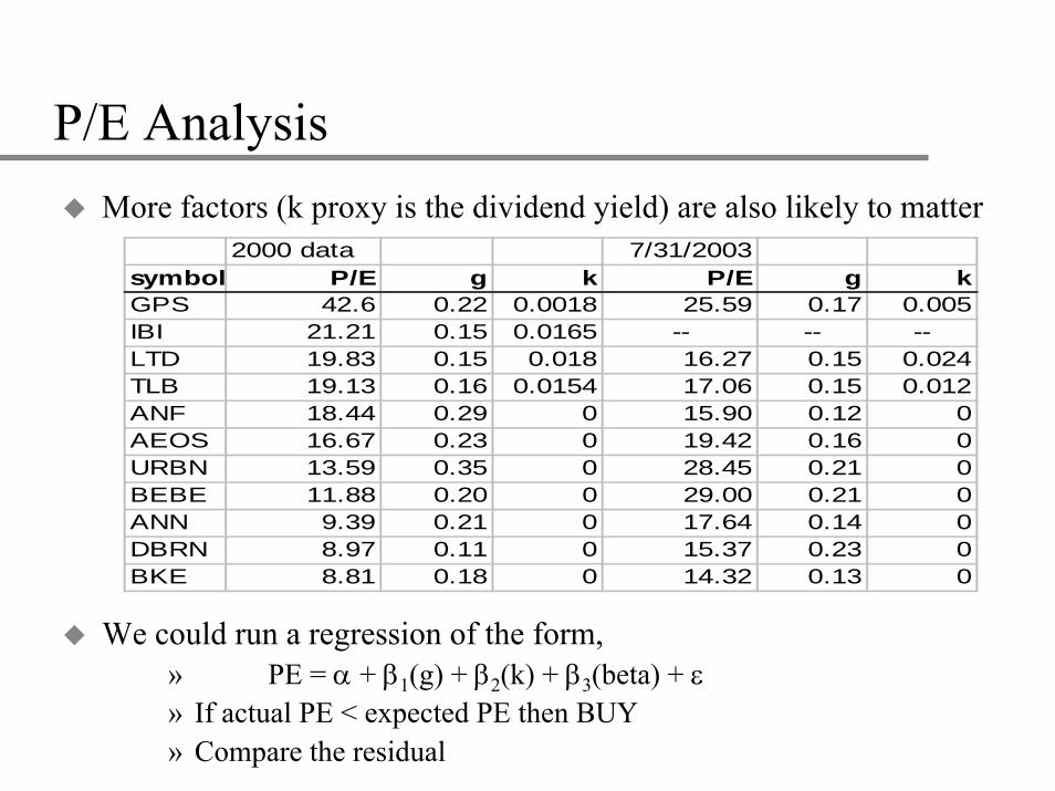
P/E AnalysisMore factors (k proxy is the dividend yield) are also likely to matter

We could run a regression of the form,» PE = α + β1(g) + β2(k) + β3(beta) + ε» If actual PE < expected PE then BUY» Compare the residual

2000 data 7/31/2003symbol P/E g k P/E g kGPS 42.6 0.22 0.0018 25.59 0.17 0.005IBI 21.21 0.15 0.0165 -- -- --LTD 19.83 0.15 0.018 16.27 0.15 0.024TLB 19.13 0.16 0.0154 17.06 0.15 0.012ANF 18.44 0.29 0 15.90 0.12 0AEOS 16.67 0.23 0 19.42 0.16 0URBN 13.59 0.35 0 28.45 0.21 0BEBE 11.88 0.20 0 29.00 0.21 0ANN 9.39 0.21 0 17.64 0.14 0DBRN 8.97 0.11 0 15.37 0.23 0BKE 8.81 0.18 0 14.32 0.13 0

P/E AnalysisRegression on g and k

2/14/2000 7/31/2003symbol P/E Predicted Residual P/E Predicted ResidualGPS 42.60 17.21 25.39 25.59 15.74 9.85IBI 21.21 15.37 5.84 -- -- --LTD 19.83 15.12 4.71 16.27 15.16 1.11TLB 19.13 15.58 3.55 17.06 15.13 1.93ANF 18.44 19.18 -0.74 15.90 14.49 1.41AEOS 16.67 17.57 -0.90 19.42 15.60 3.82URBN 13.59 20.83 -7.24 28.45 16.77 11.68BEBE 11.88 16.62 -4.74 29.00 16.94 12.06ANN 9.39 17.00 -7.61 17.64 15.07 2.57DBRN 8.97 14.21 -5.24 15.37 17.35 -1.98BKE 8.81 16.00 -7.19 14.32 14.68 -0.36

P/E RegressionsRegression on g, k, and beta

2000 data 7/31/2003

symbol P/E Predicted Residual P/E Predicted ResidualGPS 42.60 17.21 25.39 25.59 18.01 7.58IBI 21.21 15.37 5.84 -- -- --LTD 19.83 15.12 4.71 16.27 18.77 -2.50TLB 19.13 15.58 3.55 17.06 19.28 -2.22ANF 18.44 19.18 -0.74 15.90 20.58 -4.68AEOS 16.67 17.57 -0.90 19.42 21.97 -2.55URBN 13.59 20.83 -7.24 28.45 20.54 7.91BEBE 11.88 16.62 -4.74 29.00 22.41 6.59ANN 9.39 17.00 -7.61 17.64 19.09 -1.45DBRN 8.97 14.21 -5.24 15.37 -- --BKE 8.81 16.00 -7.19 14.32 16.08 -1.76

P/E Analysis - Regression ScreensBasic Steps in Regression Screens1. Use all firms in industry/sector/universe –2. Regress P/E on its underlying parameters

From Damodaran Table 8.2, using March 1997 data on 1,400 firms

P/E = 11.07 +27.8(g) + 0.73(k) + 2.94 (beta)3. Examine errors

» +ε implies overvalued» - ε implies undervalued

Problems– Regressions only use those stocks with a P/E ratio

» sample does not include negative earners– Persistence of errors...

Evidence from 2000 AnalysisGPS appeared to be overvaluedURBN, ANN, DBRN and BKE may be undervalued.What actually happened?6 mos.18 mos. 30 mos. 48 mos. 68 mos.

Sell GPS -58% -72% -72% -62% -61%Buy URBN -10% 61% 93% 244% 2059%Buy ANN 102% 43% 80% 122% 240%Buy BKE -20% 37% 28% 39% 160%Buy DBRN 78% 58% 102% 80% 291%Buy BEBE 49% 188% 28% 112% 364%

OthersLTD -7% -16% -13% 6% 51%AEOS 37% 44% -4% 30% 190%TLB 94% 118% 85% 91% 68%ANF 59% 108% 57% 220% 318%

Evidence from 2003 AnalysisGPS, URBN and BEBE appeared to be overvaluedWhat actually happened? 6 mos. 12 mos. 18 mos. 27 mos.

Sell GPS 12% 28% 20% -22%Sell URBN 114% 199% 337% 84%Sell BEBE 27% 30% 190% 54%

ANF and maybe AEOS, DBRN and LTD were undervalued.Buy ANF -12% 16% 73% 47%Buy DBRN? 18% 28% 47% 54%Buy AEOS? -5% 48% 132% 55%Buy LTD? 15% 25% 58% 30%

OthersTLB 2% -6% -11% -13%ANN 56% 43% 19% 35%BKE 27% 37% 50% 47%