![Generalized Linear Models: [3mm] An Introduction based on ... · generalized linear models (GLM’s). This class extends the class of linear models (LM’s) to regression models for](https://static.fdocuments.net/doc/165x107/5e178400e66a6a4247670a05/generalized-linear-models-3mm-an-introduction-based-on-generalized-linear.jpg)
BMI II SS06 – Class 2 “Linear Systems 2” Slide 1 Biomedical Imaging II Class 2 –...
63
BMI II SS06 – Class 2 “Linear Systems 2” Slide 1 Biomedical Imaging II Class 2 – Mathematical Preliminaries: Signal Transfer and Linear Systems Theory 2/6/06
-
Upload
alberta-hicks -
Category
Documents
-
view
215 -
download
0
Transcript of BMI II SS06 – Class 2 “Linear Systems 2” Slide 1 Biomedical Imaging II Class 2 –...

BMI II SS06 – Class 2 “Linear Systems 2” Slide 1
Biomedical Imaging IIBiomedical Imaging II
Class 2 – Mathematical Preliminaries: Signal Transfer and Linear Systems Theory
2/6/06

BMI II SS06 – Class 2 “Linear Systems 2” Slide 2
Class objectivesClass objectives
Topics you should be familiar with after lecture:
Impulse response function (irf) of a linear system (LS)
Convolutions
Fourier transform (FT)
BMI II SS06 – Class 2 “Linear Systems 2” Slide 3
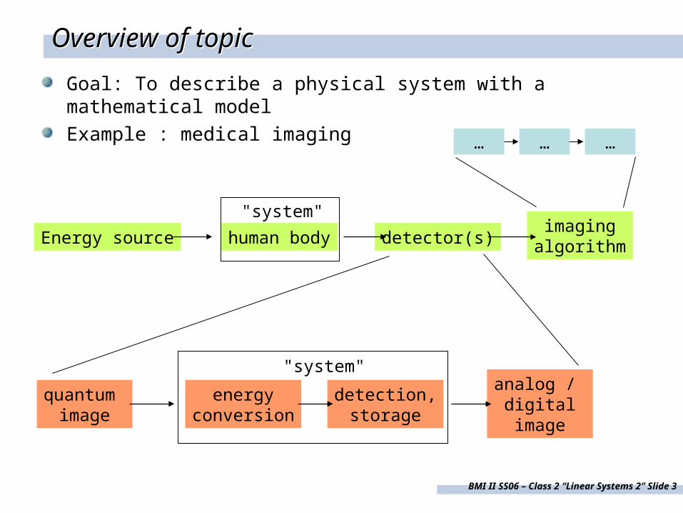
Overview of topicOverview of topic
Goal: To describe a physical system with a mathematical model
Example : medical imaging
Energy source detector(s)human body
"system"
quantum image
energyconversion
analog / digitalimage
detection,storage
"system"
imagingalgorithm
… … …
BMI II SS06 – Class 2 “Linear Systems 2” Slide 4
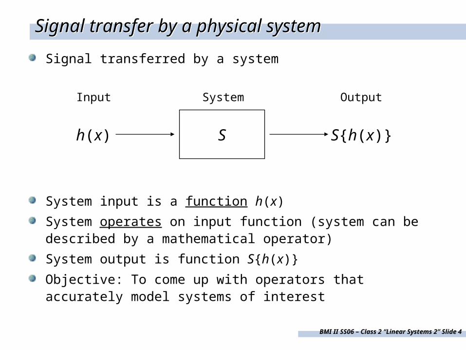
Signal transfer by a physical systemSignal transfer by a physical system
Signal transferred by a system
System input is a function h(x)
System operates on input function (system can be described by a mathematical operator)
System output is function S{h(x)}
Objective: To come up with operators that accurately model systems of interest
Sh(x) S{h(x)}
Input System Output
BMI II SS06 – Class 2 “Linear Systems 2” Slide 5
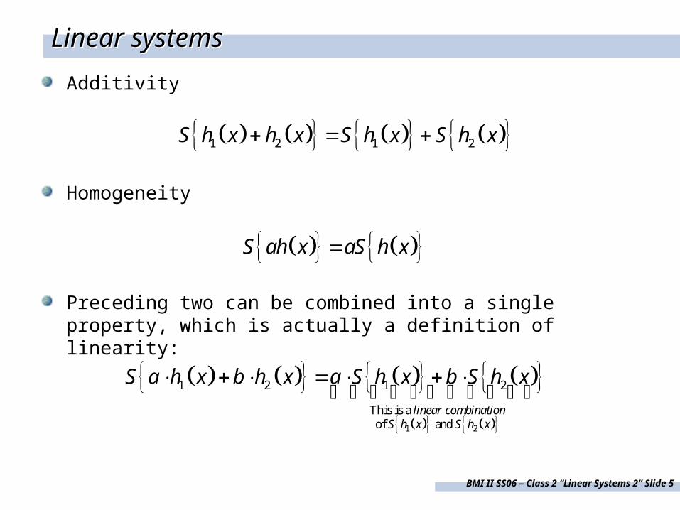
Linear systemsLinear systems
Additivity
Homogeneity
Preceding two can be combined into a single property, which is actually a definition of linearity:
1 2 1 2S h x h x S h x S h x
S ah x aS h x
1 2
1 2 1 2
This is a of and
linear combinationS h x S h x
S a h x b h x a S h x b S h x

BMI II SS06 – Class 2 “Linear Systems 2” Slide 6
LS significance and validityLS significance and validity
Why is it desirable to deal with LS?
Decomposition (analysis) and superposition (synthesis) of signals
System acts individually on signal components
No signal “mixing”
Simplifies qualitative and quantitative measurements
Lets us separate S{h(x)} into two independent factors: the source, or driving, term, and the system’s impulse response function (irf)

BMI II SS06 – Class 2 “Linear Systems 2” Slide 7
Rectangular input function (Rectangular pulse)Rectangular input function (Rectangular pulse)
Sh(x) S{h(x)}
Input System Output
h(x),h(t)
x, t
0

BMI II SS06 – Class 2 “Linear Systems 2” Slide 8
Important rectangular pulse special casesImportant rectangular pulse special cases
H(x-x0), H(t-t0)
x, t
0
Step function,Heaviside function
(1)
x0, t0
u(x), u(t)
x, t
0
x1, t1 x2, t2
(x2-x1)-1,(t2-t1)-1
Unit rectangular(or square) pulse
BMI II SS06 – Class 2 “Linear Systems 2” Slide 9
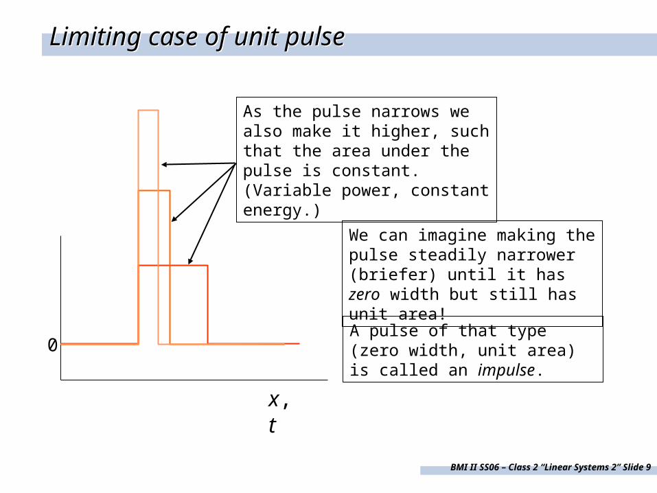
Limiting case of unit pulseLimiting case of unit pulse
x, t
0
As the pulse narrows we also make it higher, such that the area under the pulse is constant. (Variable power, constant energy.)
We can imagine making the pulse steadily narrower (briefer) until it has zero width but still has unit area!
A pulse of that type (zero width, unit area) is called an impulse.

BMI II SS06 – Class 2 “Linear Systems 2” Slide 10
Impulse response function (irf)Impulse response function (irf)
Sh(x) S{h(x)}
Input System Output
impulse function goes in… impulse response function (irf) comes out!
Note: irf has finite duration. Any input function whose width/duration is << that of the irf is effectively an impulse with respect to that system. But the same input might not be an impulse wrt a different system.

BMI II SS06 – Class 2 “Linear Systems 2” Slide 11
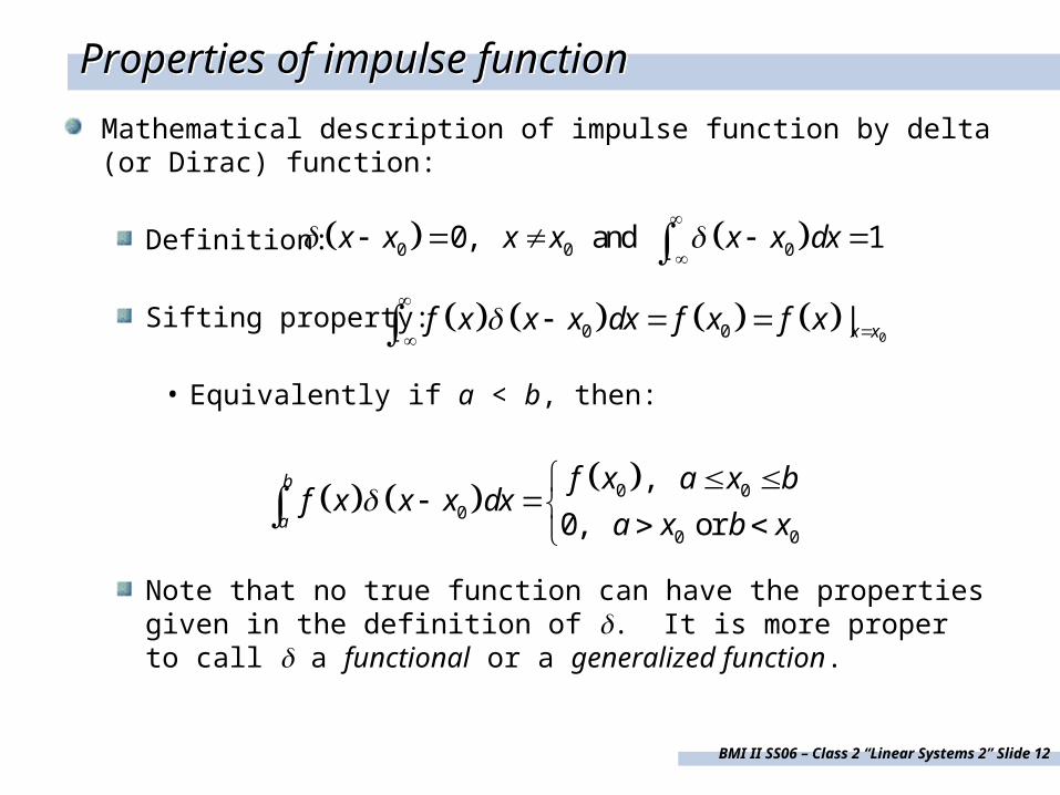
Properties of impulse functionProperties of impulse function
Mathematical description of impulse function by delta (or Dirac) function:
Definition:
Sifting property:
0 0 00, and 1x x x x x x dx
00 0 |x xf x x x dx f x f x
0
0
0
0
0
0
0
0
0
0
0 00
1
2
1
21
2
22 2
x
x
x
x
x
x
x
x
f x x x dx f x dx
f x dx
f x dx
f x f xdx f x
BMI II SS06 – Class 2 “Linear Systems 2” Slide 12
Properties of impulse functionProperties of impulse function
Mathematical description of impulse function by delta (or Dirac) function:
Definition:
Sifting property:
• Equivalently if a < b, then:
Note that no true function can have the properties given in the definition of . It is more proper to call a functional or a generalized function.
0 0 00, and 1x x x x x x dx
00 0 |x xf x x x dx f x f x
0 00
0 0
,
0, or
b
a
f x a x bf x x x dx
a x b x

BMI II SS06 – Class 2 “Linear Systems 2” Slide 13
Relation between impulse and step functionsRelation between impulse and step functions
0 0 0 0,d
t t H t t H t t t t dtdt
H(x-x0), H(t-t0)
x, t
0
Step function,Heaviside function
(1)
x0, t0
BMI II SS06 – Class 2 “Linear Systems 2” Slide 14
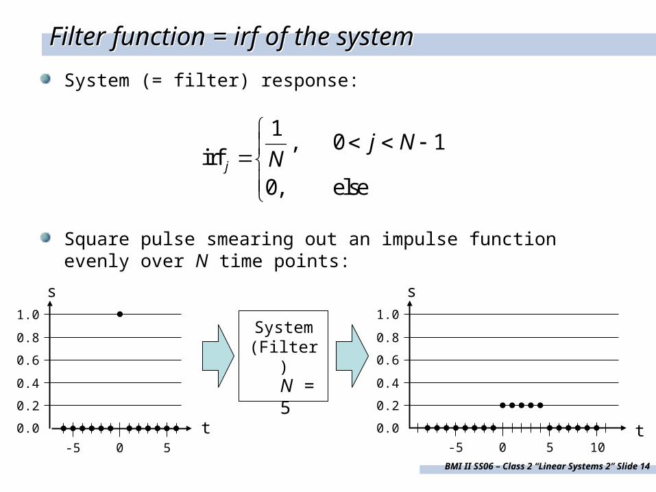
Filter function = irf of the systemFilter function = irf of the system
System (= filter) response:
Square pulse smearing out an impulse function evenly over N time points:
1, 0 1
irf0, else
j
j NN
N = 5
0 5-5
t
0.2
0.4
0.0
0.6
0.8
1.0
s
System(Filter)
0 5 10-5t
0.2
0.4
0.0
0.6
0.8
1.0
s

BMI II SS06 – Class 2 “Linear Systems 2” Slide 15
Output for arbitrary input signals is given by superposition principle (Linearity!)
Think of an arbitrary input function as a sequence of impulse functions, of varying strengths (areas), tightly packed together
Then the defining property of an LS, (S{a·h1 + b·h2} = a·S{h1} + b·S{h2}) tells us that the overall system response is the sum of the corresponding irfs, properly scaled and shifted.
Significance of the irf of a LSSignificance of the irf of a LS
=

BMI II SS06 – Class 2 “Linear Systems 2” Slide 16
Significance of the irf of a LSSignificance of the irf of a LS
To state the same idea mathematically, LS output given by convolution of input signal and irf:
' irf ' ' irfS h x d x h x x x dx h x x
Notice that the sum of these two arguments is a constant
or t

BMI II SS06 – Class 2 “Linear Systems 2” Slide 17
1/6
1 2 3 4 5 6
1/6
2 3 4 5 6 7 8 9 10 11 12
Real-world convolution example
BMI II SS06 – Class 2 “Linear Systems 2” Slide 18
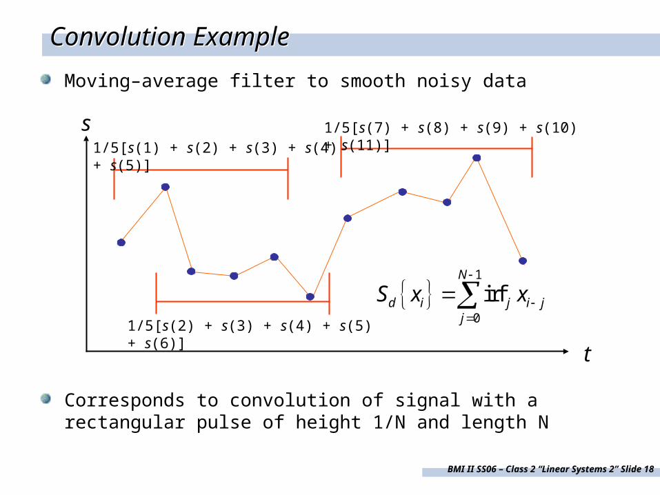
Convolution ExampleConvolution Example
Moving–average filter to smooth noisy data
Corresponds to convolution of signal with a rectangular pulse of height 1/N and length N
t
s1/5[s(1) + s(2) + s(3) + s(4) + s(5)]
1/5[s(2) + s(3) + s(4) + s(5) + s(6)]
1/5[s(7) + s(8) + s(9) + s(10) + s(11)]
1
0
irfN
d i j i jj
S x x
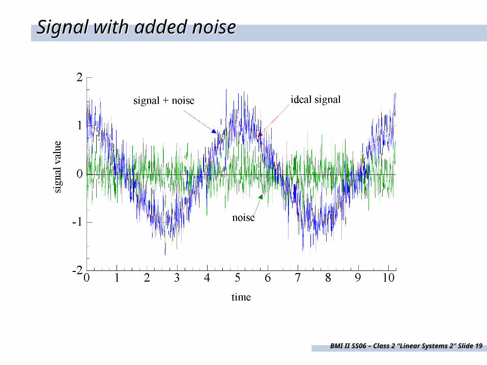
BMI II SS06 – Class 2 “Linear Systems 2” Slide 19
Signal with added noiseSignal with added noise

BMI II SS06 – Class 2 “Linear Systems 2” Slide 20
Result of smoothingResult of smoothing

BMI II SS06 – Class 2 “Linear Systems 2” Slide 21
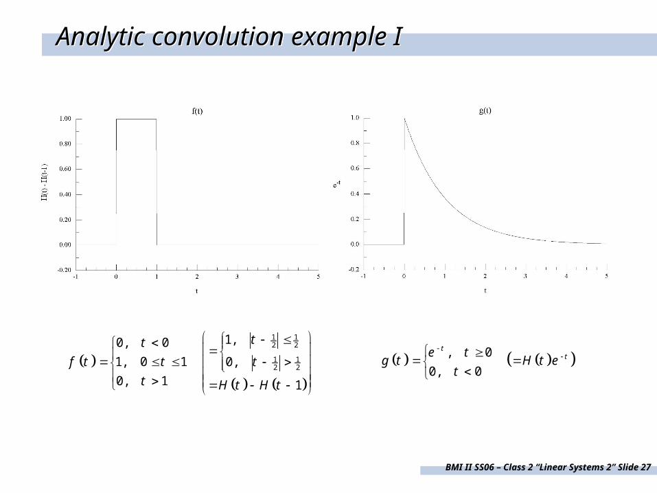
Analytic convolution example IAnalytic convolution example I
1 12 2
1 12 2
1,0, 0
1, 0 1 0,
0, 1 1
tt
f t t t
t H t H t
, 0
0, 0
tte t
g t H t et
BMI II SS06 – Class 2 “Linear Systems 2” Slide 22
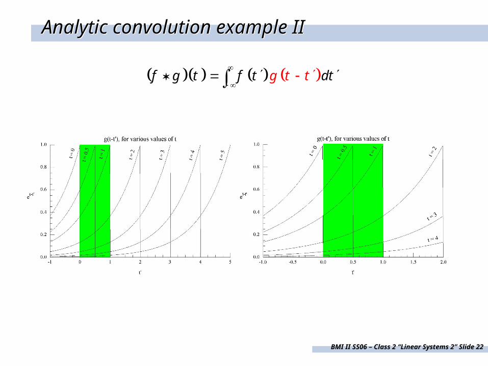
g t tf g t f t dt
Analytic convolution example IIAnalytic convolution example II
BMI II SS06 – Class 2 “Linear Systems 2” Slide 23
0 1
0 1
1
0
0 1 0
t
t
t t t
t t t
t
t
f g t f t g t t dt
g t t dt g t t dt g t t dt
g t t dt
,
0 , 1 1
u t t du dt
t u t t u t
1
01
1
0, 0
, 0 1
, 1
u t u tt u
u t u tt u
t
t
f g t g u du g u du e du t
e du t
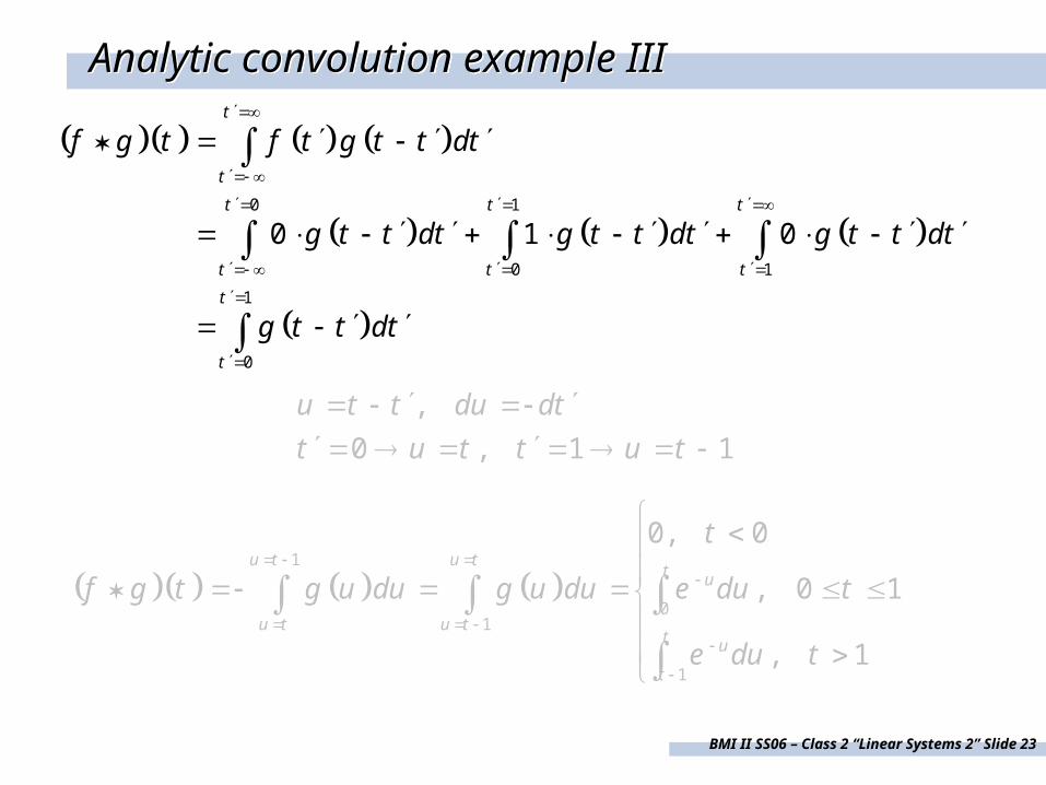
Analytic convolution example IIIAnalytic convolution example III
BMI II SS06 – Class 2 “Linear Systems 2” Slide 24
0 1
0 1
1
0
0 1 0
t
t
t t t
t t t
t
t
f g t f t g t t dt
g t t dt g t t dt g t t dt
g t t dt
,
0 , 1 1
u t t du dt
t u t t u t
1
01
1
0, 0
, 0 1
, 1
u t u tt u
u t u tt u
t
t
f g t g u du g u du e du t
e du t
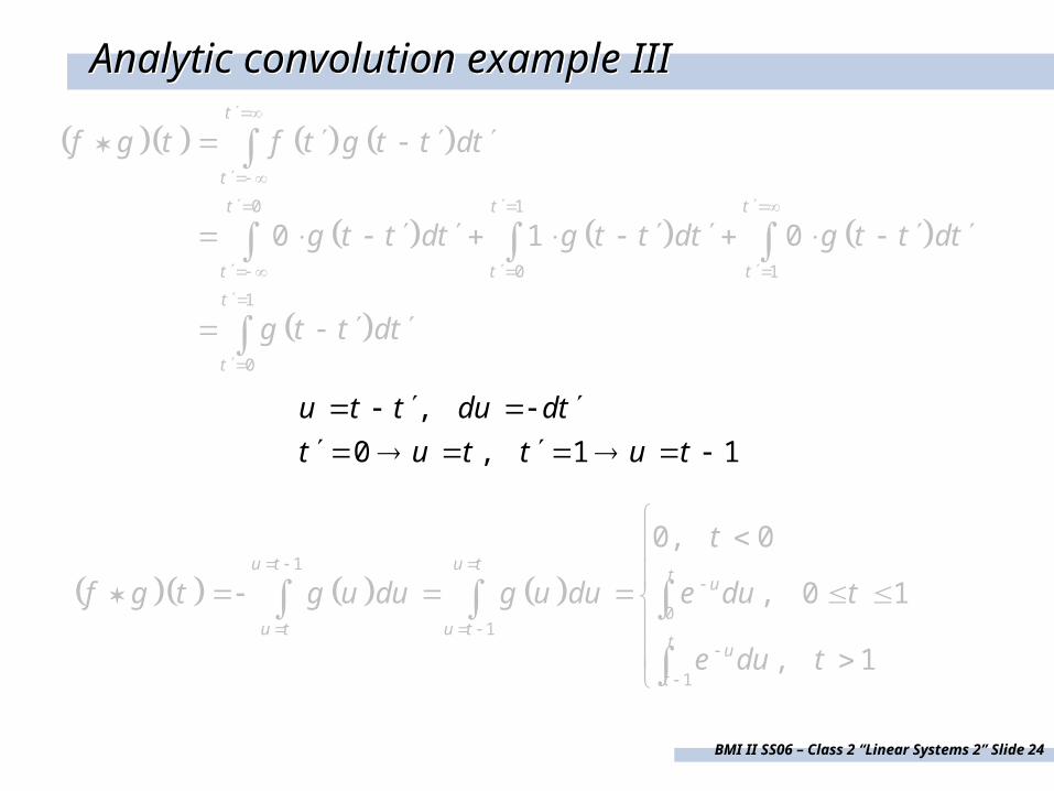
Analytic convolution example IIIAnalytic convolution example III

BMI II SS06 – Class 2 “Linear Systems 2” Slide 25
0 1
0 1
1
0
0 1 0
t
t
t t t
t t t
t
t
f g t f t g t t dt
g t t dt g t t dt g t t dt
g t t dt
,
0 , 1 1
u t t du dt
t u t t u t
1
01
1
0, 0
, 0 1
, 1
u t u tt u
u t u tt u
t
t
f g t g u du g u du e du t
e du t
Analytic convolution example IIIAnalytic convolution example III
BMI II SS06 – Class 2 “Linear Systems 2” Slide 26
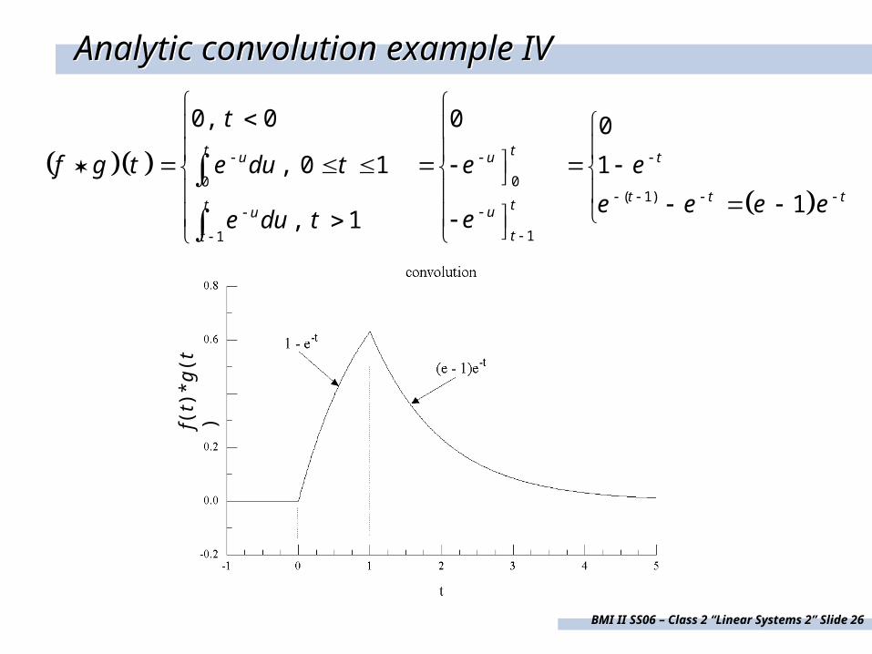
00( 1)
11
0, 0 0 0
, 0 1 1
1, 1
t tu u t
t t ttt uu
tt
t
f g t e du t e e
e e e eee du t
f(t)
*g(t
)
Analytic convolution example IVAnalytic convolution example IV
BMI II SS06 – Class 2 “Linear Systems 2” Slide 27
Analytic convolution example IAnalytic convolution example I
1 12 2
1 12 2
1,0, 0
1, 0 1 0,
0, 1 1
tt
f t t t
t H t H t
, 0
0, 0
tte t
g t H t et
BMI II SS06 – Class 2 “Linear Systems 2” Slide 28
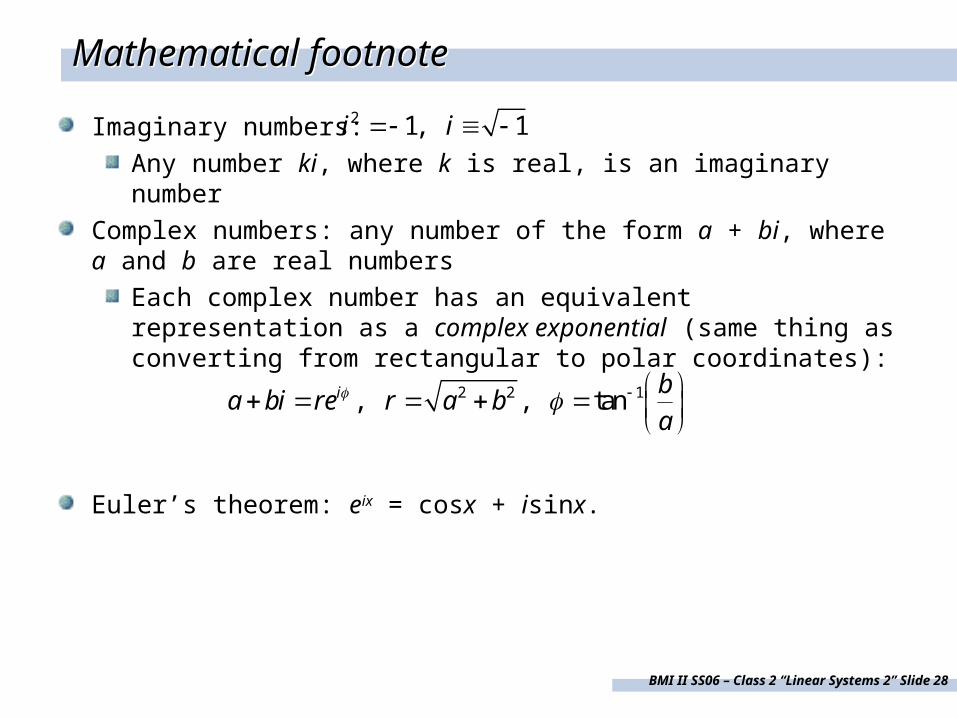
Mathematical footnoteMathematical footnote
Imaginary numbers:
Any number ki, where k is real, is an imaginary number
Complex numbers: any number of the form a + bi, where a and b are real numbers
Each complex number has an equivalent representation as a complex exponential (same thing as converting from rectangular to polar coordinates):
Euler’s theorem: eix = cosx + isinx.
2 1, 1i i
2 2 1, , tani ba bi re r a b
a
BMI II SS06 – Class 2 “Linear Systems 2” Slide 29
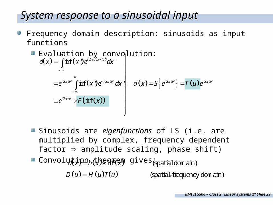
System response to a sinusoidal inputSystem response to a sinusoidal input
Frequency domain description: sinusoids as input functions
Evaluation by convolution:
Sinusoids are eigenfunctions of LS (i.e. are multiplied by complex, frequency dependent factor amplitude scaling, phase shift)
Convolution theorem gives:
2 '
2 2 ' 2 2
2
irf ' '
irf ' '
irf
i u x x
i ux i ux i ux i ux
i ux
d x x e dx
e x e dx d x S e T u e
e x
F
irf (spatial domain)
(spatial-frequency domain)
d x h x x
D u H u T u

BMI II SS06 – Class 2 “Linear Systems 2” Slide 30
Excursion: Fourier Transform (FT)Excursion: Fourier Transform (FT)
The one-dimensional Fourier Transform is given by
F() is in general a complex number, with real and imaginary parts
Mostly interested in magnitude or power (= M()2 = |F()|2) of FT (the spectrum of f(t))
cos sini tF f t e dt f t t i t dt
F R iI
, Magnitude
Phase tan
iM e M R I
I
R
2 2
1

BMI II SS06 – Class 2 “Linear Systems 2” Slide 31
Inverse FTInverse FT
The one-dimensional inverse Fourier Transform (IFT) is given by
cos sin
i tf t F e d
F t i t d
1212
The Fourier transform and its inverse can be interpreted as a mathematical technique for converting time–domain data to frequency–domain data, and vice versa.
BMI II SS06 – Class 2 “Linear Systems 2” Slide 32
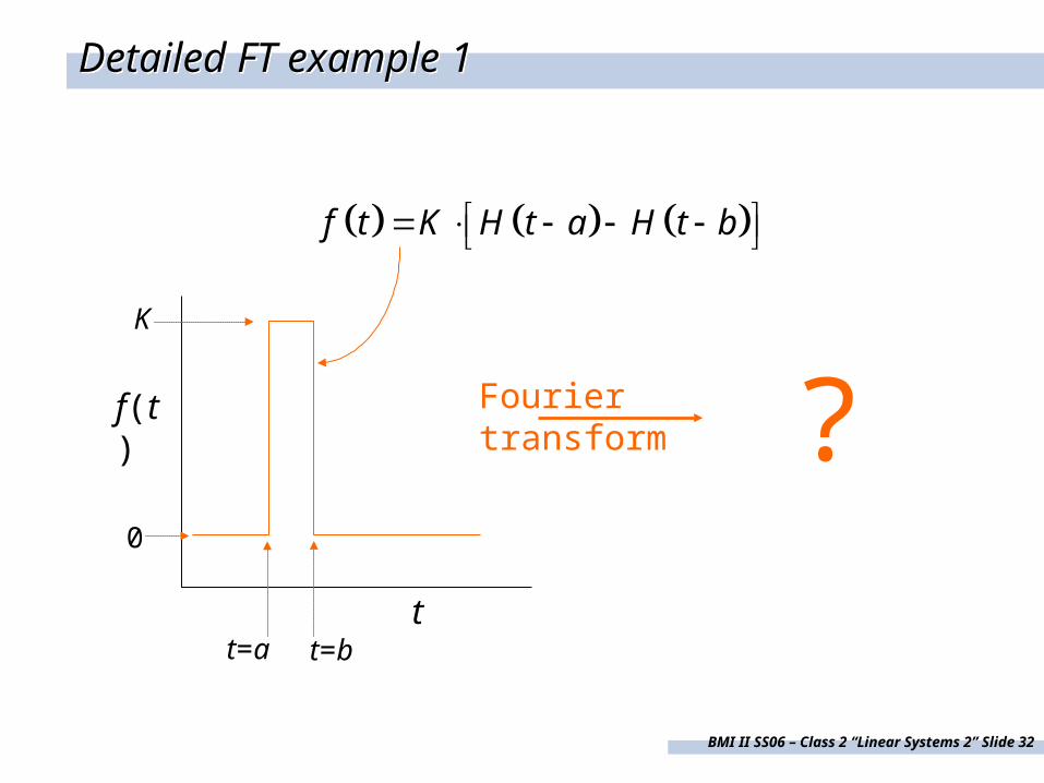
Detailed FT example 1Detailed FT example 1
t
f(t)
t=a t=b
K
0
Fourier transform ?
f t K H t a H t b

BMI II SS06 – Class 2 “Linear Systems 2” Slide 33
sin sin cos cos
t bt bi t i t
t at a
ib ia
KF F f t K e dt e
i
Kie e
Kb a i b a
a = 0.9, b = 1.1, K = 2 a = 0.4, b = 0.6, K = 2
MM
M(F) M(F)
ω ω
Detailed FT example 1Detailed FT example 1
BMI II SS06 – Class 2 “Linear Systems 2” Slide 34
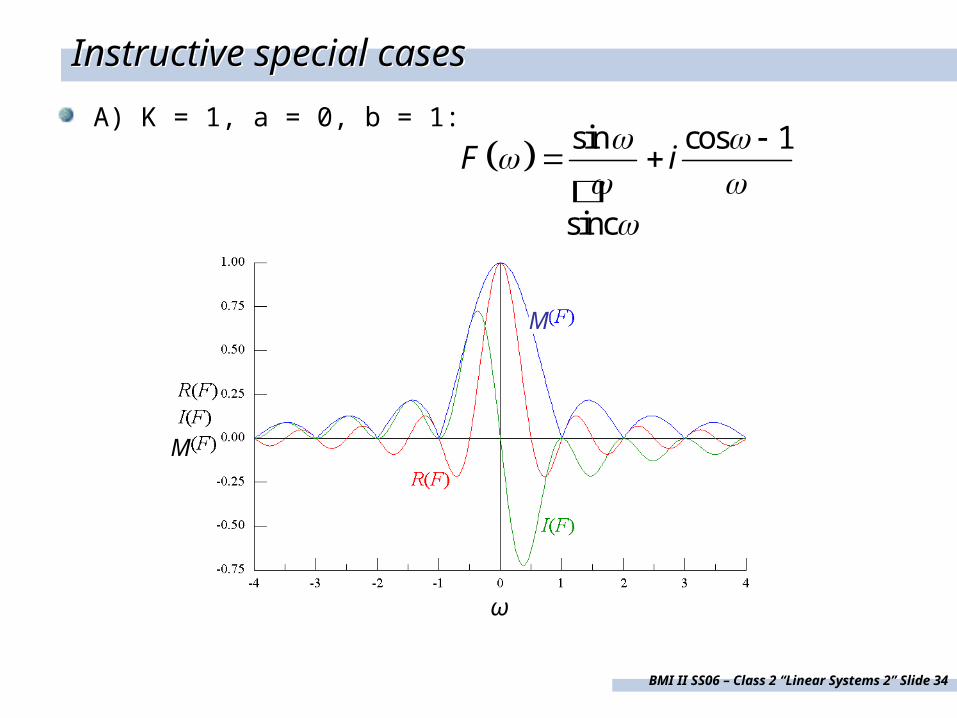
Instructive special casesInstructive special cases
A) K = 1, a = 0, b = 1:
sin cos 1
sinc
F i
M
M
ω

BMI II SS06 – Class 2 “Linear Systems 2” Slide 35
Result of smoothingResult of smoothing
BMI II SS06 – Class 2 “Linear Systems 2” Slide 36
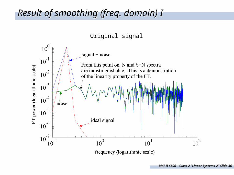
Result of smoothing (freq. domain) IResult of smoothing (freq. domain) I
Original signal
BMI II SS06 – Class 2 “Linear Systems 2” Slide 37
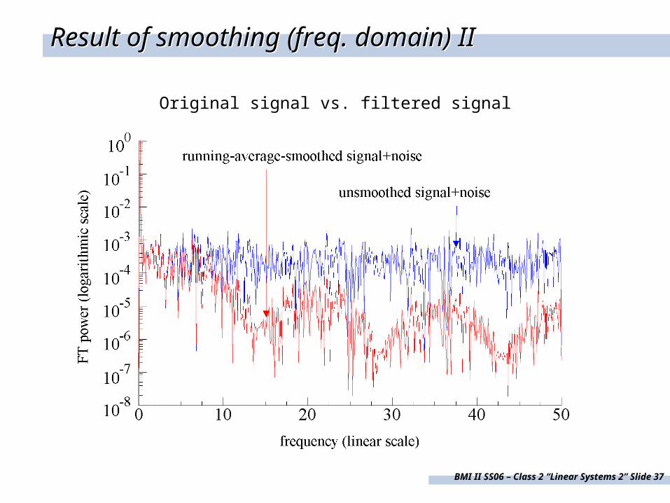
Original signal vs. filtered signal
Result of smoothing (freq. domain) IIResult of smoothing (freq. domain) II
BMI II SS06 – Class 2 “Linear Systems 2” Slide 38
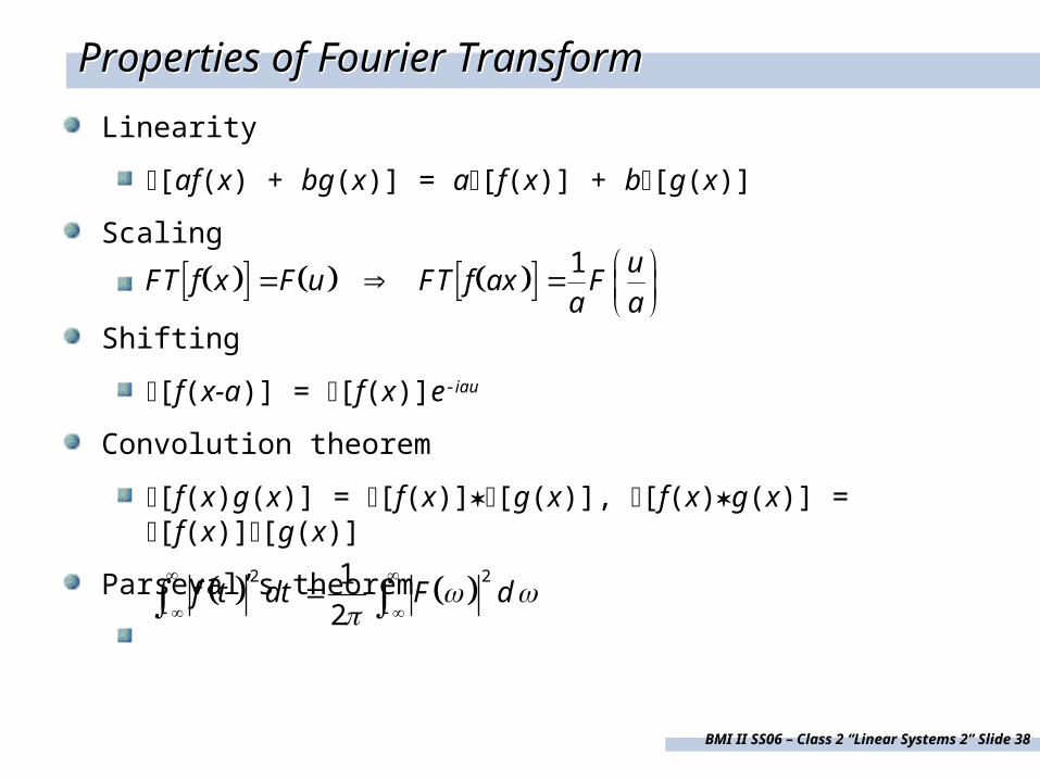
Properties of Fourier TransformProperties of Fourier Transform
Linearity
[af(x) + bg(x)] = a[f(x)] + b[g(x)]
Scaling
Shifting
[f(x-a)] = [f(x)]e-iau
Convolution theorem
[f(x)g(x)] = [f(x)][g(x)], [f(x)g(x)] = [f(x)][g(x)]
Parseval’s theorem
1 u
FT f x F u FT f ax Fa a
2 212
f t dt F d
BMI II SS06 – Class 2 “Linear Systems 2” Slide 39
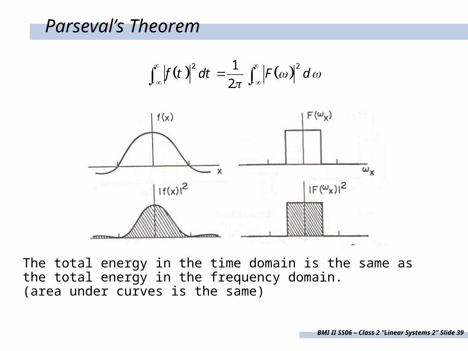
Parseval’s Theorem
2 212
f t dt F d
The total energy in the time domain is the same as the total energy in the frequency domain. (area under curves is the same)
BMI II SS06 – Class 2 “Linear Systems 2” Slide 40
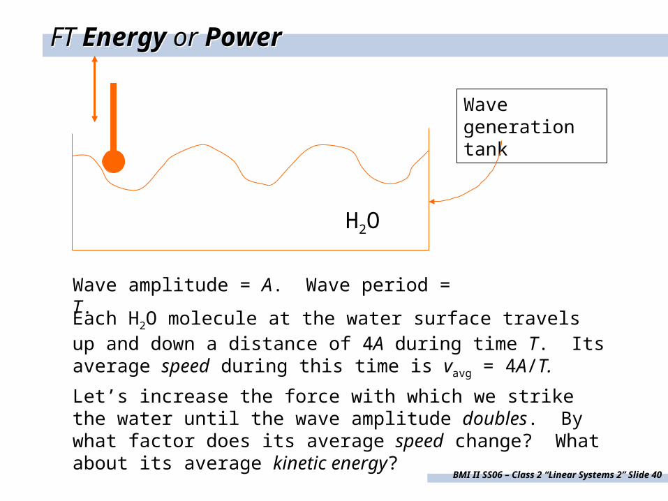
FT Energy or Power FT Energy or Power
H2O
Wave generation tank
Each H2O molecule at the water surface travels up and down a distance of 4A during time T. Its average speed during this time is vavg = 4A/T.
Wave amplitude = A. Wave period = T.
Let’s increase the force with which we strike the water until the wave amplitude doubles. By what factor does its average speed change? What about its average kinetic energy?

BMI II SS06 – Class 2 “Linear Systems 2” Slide 41
Class objectivesClass objectives
Topics you should be familiar with after lecture:
FT of an impulse (delta) function
FT of a sequence of impulses
Equivalence of a discrete (or sampled) function to the product of a continuous function and a “comb” of impulses
Relationship between FT of a discrete function and the continuous function from which it is obtained
Formulas for discrete Fourier transform (DFT)
Essential properties of DFT, and differences between DFT and continuous FT
What aliasing is
What a band-limited function is
Definition of correlation
Relationships/differences between correlation and convolution

BMI II SS06 – Class 2 “Linear Systems 2” Slide 42
Impulse function FTImpulse function FT
0 0t t f t dt f t
0
0 0
0 0
10
12
i ti t
i t i t i t
t t e dt e F t t
F e e e d t t
0 0
02i t i t i tF e e e dt
1F 2
F t 1

BMI II SS06 – Class 2 “Linear Systems 2” Slide 43
FT of multiple impulse functionsFT of multiple impulse functions
0 1 2
0 1 2i t
i t i t i t
t t t t t t e dt
e e e
But what does an FT of this sort look like?Comb
function
t0 = 0
t0 = 1t0 = -1
t0 = 2t0 = -2

BMI II SS06 – Class 2 “Linear Systems 2” Slide 44
Partial sums of comb function FTPartial sums of comb function FT
0 2 4 6 8 10 12 14
R(F
T)
-2
-1
0
1
2
3
4
5
0 2 4 6 8 10 12 14
R(F
T)
-10
-6
-2
2
6
10
14
18
22
26
30
34
38
42

BMI II SS06 – Class 2 “Linear Systems 2” Slide 45
Comb function FTComb function FT
Time Domain: Comb of -functions separated by T.
Frequency Domain: Comb of -functions with separation 1/T.
f

BMI II SS06 – Class 2 “Linear Systems 2” Slide 46
Analytic, continuous-function FT exampleAnalytic, continuous-function FT example
FT
BMI II SS06 – Class 2 “Linear Systems 2” Slide 47
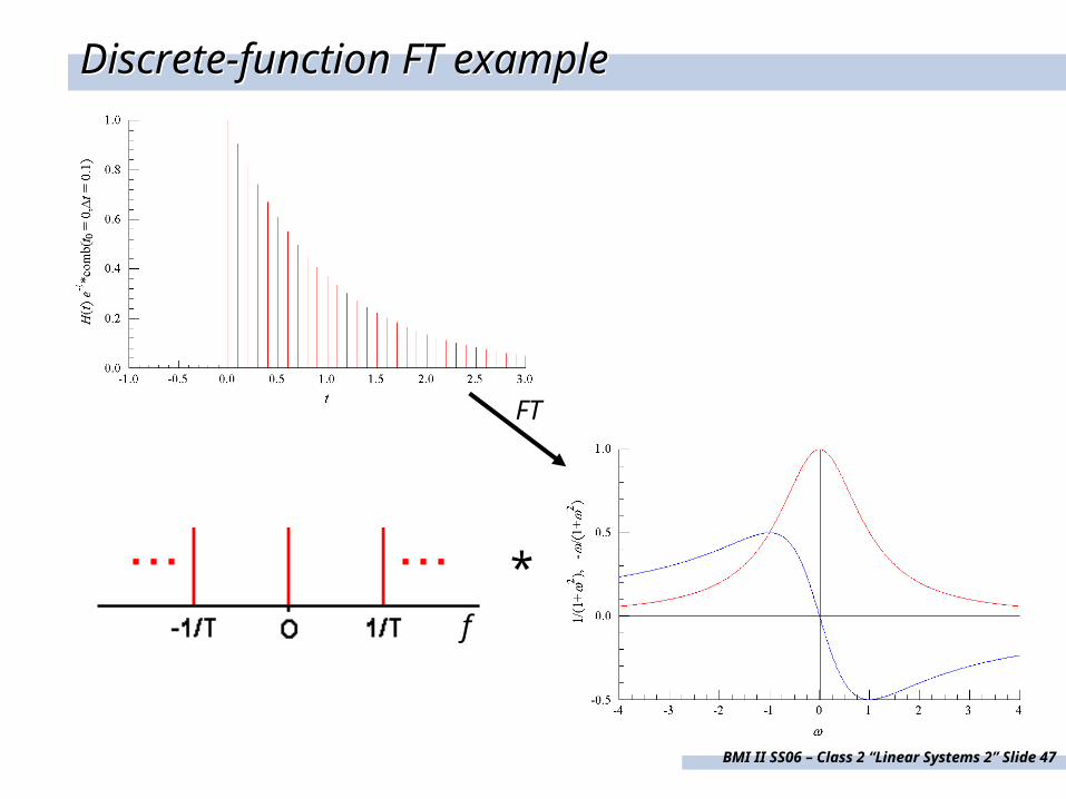
f
*
Discrete-function FT exampleDiscrete-function FT example
FT

BMI II SS06 – Class 2 “Linear Systems 2” Slide 48
Convolution of comb and non-periodic FTConvolution of comb and non-periodic FT

BMI II SS06 – Class 2 “Linear Systems 2” Slide 49
Discrete Fourier Transform (DFT)In real life, data are typically sampled at N evenly spaced time intervals Δt.
To take Fourier Transform of discretely sampled signals, we need the DFT of a sequence {u(n), n = 0, 1, ...., N-1}
21
0
1, 0, 1, ... , 2.
iN knN
n
v k u n e k NN
The inverse discrete Fourier Transform is given by
22
0
1, 0, 1, ... , 1.
iN knN
k
u n v k e n NN

BMI II SS06 – Class 2 “Linear Systems 2” Slide 50
DFT – What happens when k = 0 or N/2 ?
21 10 0
0 0
1
0
1 10
1
iN NnN
n n
N
n
v u n e u n eN N
u nN
21 12
0 0
1
0
1 12
11
i NN Nn inN
n n
Nn
n
Nv u n e u n e
N N
u nN
BMI II SS06 – Class 2 “Linear Systems 2” Slide 51
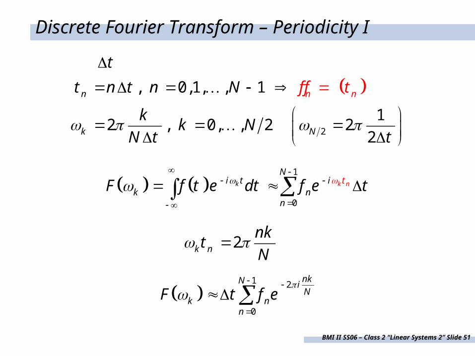
Discrete Fourier Transform – Periodicity I
1
0
kk n
Ni t i
kn
tnF f t e dt f e t
2
, 0,1, , 1
12 , 0, , 2 2
2
n
k
n
N
nff t
t
t n t n N
kk N
N t t
2k n
nkt
N
1 2
0
nkN iN
k nn
F t f e
BMI II SS06 – Class 2 “Linear Systems 2” Slide 52
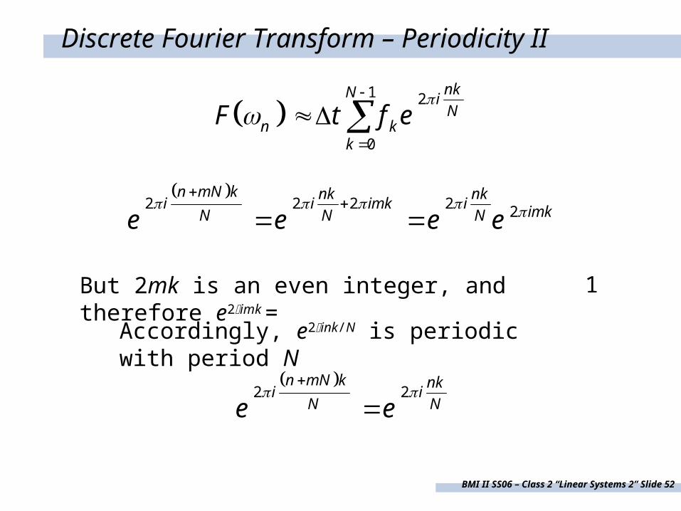
Discrete Fourier Transform – Periodicity II
1 2
0
nkN iN
n kk
F t f e
2 2 2 2 2
n mN k nk nki i imk i imkN N Ne e e e
But 2mk is an even integer, and therefore e2imk =
1
Accordingly, e2ink/N is periodic with period N
2 2
n mN k nki i
N Ne e

BMI II SS06 – Class 2 “Linear Systems 2” Slide 53
Discrete functions and aliasing IDiscrete functions and aliasing I
BMI II SS06 – Class 2 “Linear Systems 2” Slide 54
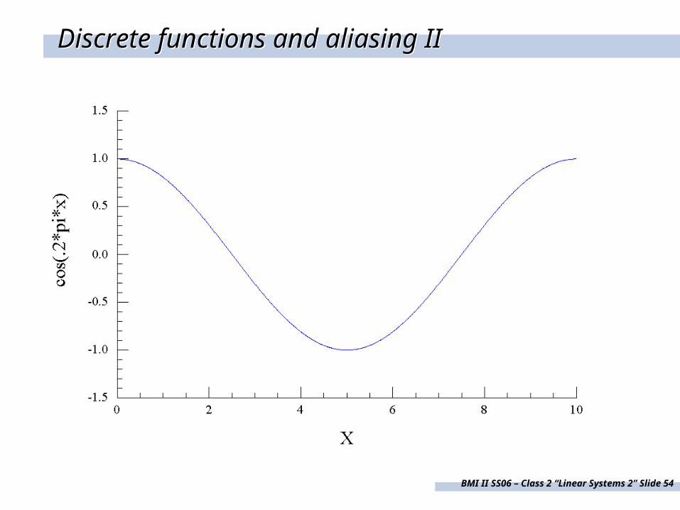
Discrete functions and aliasing IIDiscrete functions and aliasing II

BMI II SS06 – Class 2 “Linear Systems 2” Slide 55
Discrete functions and aliasing IIIDiscrete functions and aliasing III
BMI II SS06 – Class 2 “Linear Systems 2” Slide 56
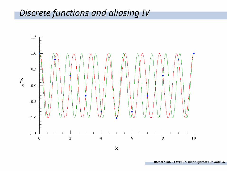
Discrete functions and aliasing IVDiscrete functions and aliasing IV
BMI II SS06 – Class 2 “Linear Systems 2” Slide 57
Discrete functions and aliasing VDiscrete functions and aliasing V
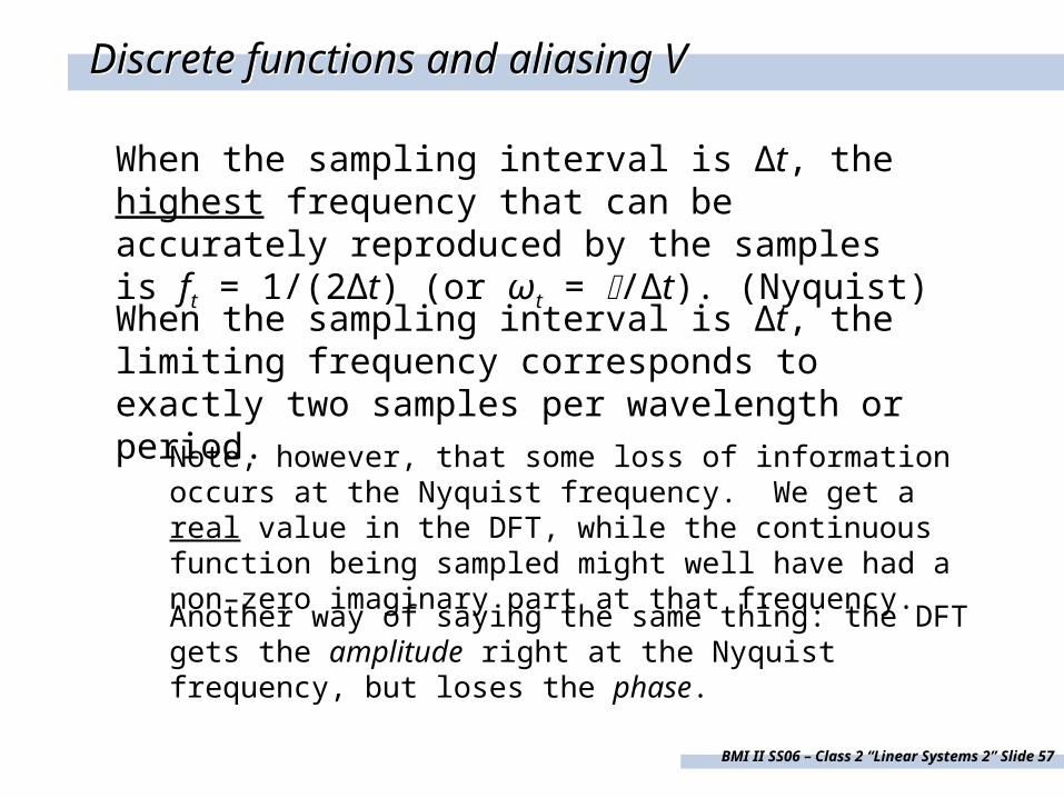
When the sampling interval is Δt, the highest frequency that can be accurately reproduced by the samples is ft = 1/(2Δt) (or ωt = /Δt). (Nyquist)When the sampling interval is Δt, the limiting frequency corresponds to exactly two samples per wavelength or period.
Note, however, that some loss of information occurs at the Nyquist frequency. We get a real value in the DFT, while the continuous function being sampled might well have had a non–zero imaginary part at that frequency.Another way of saying the same thing: the DFT gets the amplitude right at the Nyquist frequency, but loses the phase.
BMI II SS06 – Class 2 “Linear Systems 2” Slide 58
Discrete functions and aliasing VIDiscrete functions and aliasing VI
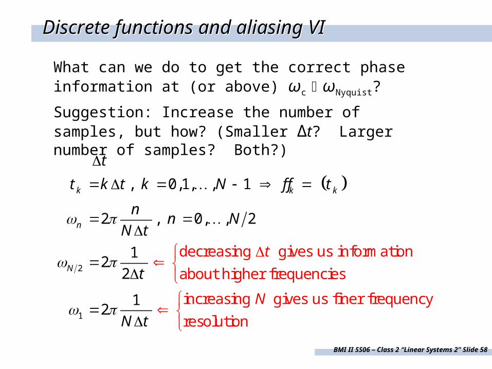
What can we do to get the correct phase information at (or above) ωc ωNyquist?
Suggestion: Increase the number of samples, but how? (Smaller Δt? Larger number of samples? Both?)
2
1
decreasing gives us information
, 0,1, , 1
2 , 0, , 2
12
2
12
about higher frequencies
increasing gives us finer frequency
resolution
k k k
n
N
t
t k t k N ff t
nn N
N t
t
N t
t
N
BMI II SS06 – Class 2 “Linear Systems 2” Slide 59
Discrete functions and aliasing VIIDiscrete functions and aliasing VII
When a continuous function is sampled at rate Δt, the DFT contains all frequencies above ωc aliased down to apparent frequencies less than ωc.
The only good (I said good, not easy) preventives for aliasing are: 1. increase sampling rate until ωc reaches a value above which it is known a priori that the continuous signal contains negligible spectral energy; 2. have the continuous signal pass through a low–pass filter, with a frequency cutoff less than ωc, before the signal is sampled.
If either of the above is successfully carried out, then the continuous signal is said to be band–limited.
BMI II SS06 – Class 2 “Linear Systems 2” Slide 60
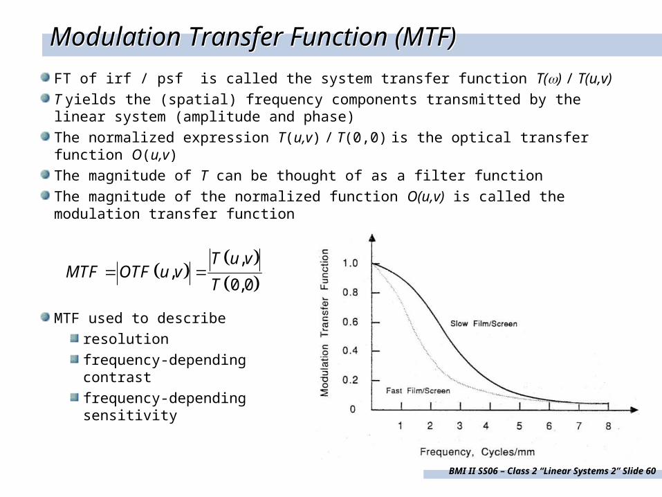
Modulation Transfer Function (MTF)Modulation Transfer Function (MTF)
FT of irf / psf is called the system transfer function T() / T(u,v)
T yields the (spatial) frequency components transmitted by the linear system (amplitude and phase)
The normalized expression T(u,v) / T(0,0) is the optical transfer function O(u,v)
The magnitude of T can be thought of as a filter function
The magnitude of the normalized function O(u,v) is called the modulation transfer function
MTF used to describe
resolution
frequency-dependingcontrast
frequency-dependingsensitivity
,,
0,0
T u vMTF OTF u v
T

BMI II SS06 – Class 2 “Linear Systems 2” Slide 61
Convolution: f t g t f g t f t g t t dt
Convolution vs. CorrelationConvolution vs. Correlation
Correlation: f t g t f g t f t g t t dt
Sum is a constant
Difference is a constant
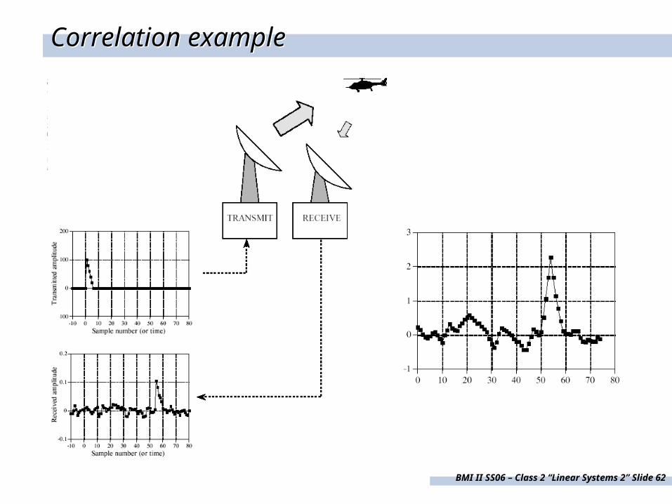
Correlation is a measure of the similarity between f and g.
t is a variable to account for the possibility that it might look as though f and g are very different, but it turns out that g is simply displaced in time relative to f.
BMI II SS06 – Class 2 “Linear Systems 2” Slide 62
Correlation exampleCorrelation example
BMI II SS06 – Class 2 “Linear Systems 2” Slide 63
Convolution: t f t g t t dtf g
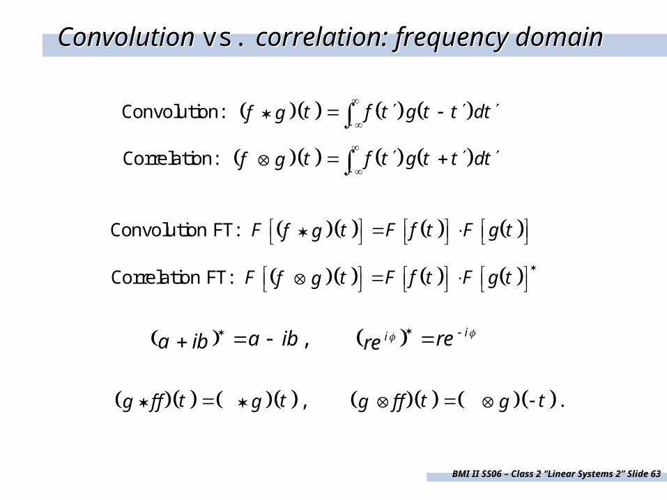
Convolution vs. correlation: frequency domainConvolution vs. correlation: frequency domain
Correlation: t f t g t t dtf g
Convolution FT: F t F f t F g tf g
Correlation FT: F t F f t F g tf g
, iia ib rea ib re
, .t t t tg ff g g ff g