40 Jahre Bluhm Systeme. 40 Jahre Innovation in der Kennzeichnung.
description

Growth Dynamics and Development
Essays in Applied Econometrics andPolitical Economy
Richard Bluhm

ISBN 978 90 8666 363 7
Copyright c© Richard Bluhm, 2015
All rights reserved. No part of this publication may be reproduced, stored in a retrieval system,or transmitted in any form, or by any means, electronic, mechanical, photocopying, recordingor otherwise, without the prior permission in writing, from the author.
Publisher: Boekenplan, Maastricht

Growth Dynamics and Development: Essays in Applied
Econometrics and Political Economy
dissertation
to obtain the degree of Doctor atMaastricht University,
on the authority of the Rector Magnificus Prof. dr. L.L.G. Soete,in accordance with the decision of the Board of Deans,
to be defended in public on Thursday, 26 March 2015, at 16:00 hours
by
Richard Bluhm

PromoterProf. Dr. Adam Szirmai
Co-SupervisorDr. Denis de Crombrugghe
Assessment CommitteeProf. Dr. Franz C. Palm (chair)Prof. Dr. Pierre MohnenDr. Toke Aidt (Cambridge University)Prof. Dr. Jakob de Haan (Rijksuniversiteit Groningen, De Nederlandsche Bank)

Acknowledgements
“Why don’t you apply in Maastricht?” These six words, spoken by Yannic Franken atthe Canadian Embassy in Berlin in early 2009, started it all. I moved to Maastricht formy masters. After a brief detour to Geneva and thanks to the generous offer of a positionfrom Chris de Neubourg as well as encouragement from Michael Cichon, I returned inthe fall of 2010 to embark on a PhD.
Many would consider themselves blessed if they had one engaged promoter orsupervisor. I had the immense pleasure to learn from, work with, and intellectually sparwith three on a regular basis. First and foremost, I would like to thank my promoterEddy Szirmai. I remember a time when I needed to convince him to supervise me. Iam glad he finally agreed, shaped this book with me, and taught me the ins and outs ofacademia in the process. Sitting directly next to Eddy, my eyes would usually find Denisde Crombrugghe. Without his guidance, support and the many challenges he gave me,I could not imagine having developed such a knack for quantitative economics. I alsowish to thank my “informal co-supervisor”, Kaj Thomsson, who inspired me to work ona political economy theory paper with him. All three gave me the greatest gift there isfor any graduate student: seemingly infinite amounts of their time.
I would also like to express gratitude to my assessment committee: Franz Palm, PierreMohnen, Toke Aidt, and Jakob de Haan. I look up to their accomplishments in so manyways. Receiving their comments on this book, together with their approval, has been anenormous joy.
I owe a deep debt to my colleagues and friends at the Agence Francaise deDeveloppement (AFD): Nicolas Meisel, Thomas Roca, Cyrille Bellier and VeroniqueSauvat. This dissertation would have never happened without their financial andintellectual support. Working with them in the ‘Institutions and Long-term Growth’project has been nothing but a rewarding experience. They also introduced me toanother set of wonderful people, such as John Wallis, Mushtaq Khan, Lawrence Haddad,Hiroshi Kato, Lawrence Chandy, Charles Kenny, Steven Webb, and countless othersduring workshops in Paris and elsewhere.
I also benefited from frequent mini-workshops together with the other project membersin Maastricht, among them were Bart Verspagen (who never failed to ask the toughestquestions), Franziska Gassmann, Thomas Ziesemer, and my extended supervisory teamof three. Furthermore, I had many exciting discussions with the other junior researcherswho graduated before me: Biniam Bedasso, Samyukta Bhupatiraju, Luciana Cingolani,and Kristine Farla. Now it is time to join your ranks.
Along the way, I met many fantastic people who took the time to discuss my papersor comment on my presentations, among them were Ajay Shah (thanks for inviting meto India), Jan Egbert-Sturm (thanks for inviting me to Zurich), Jeffrey Wooldridge, D.S.Prasada Rao, Gani Aldashev, Carmine Guerriero, Steven van de Walle, Sascha Becker,Oded Galor, Stefan Klasen, Agustin Casas, Florent Bresson and William Poulliot. I owe
v

a special thank you to Melanie Krause, who has gone through nearly all of my paperswith Argus’ eyes and never failed to find yet another typo or spot where they could beimproved. Thank you Theophile Azomahou, Raouf Boucekkine, Pierre Mohnen and BartVerspagen for inviting one of my papers to appear in a special issue of MacroeconomicDynamics.
Several people at the school made my life interesting and easier in many ways:Franziska Gassmann, Lutz Krebs, Zina Nimeh, Robin Cowan, Eveline in de Braek, Mindelvan de Laar, Susan Roggen, Howard Hudson, Janneke Knaapen and Herman Pijpers.Depending on their role, they have supported me, taught me during the first year of thePhD, helped coordinate my teaching, and helped with project websites, or (as in the caseof Susan) never failed to smile when presented with yet another administrative questionor travel claim. Thank you!
I am also indebted to Martin Gassebner who made my transition into the (post-doctoral) “afterlife” so seamless by offering me a great job. I am glad he is joining thefestivities celebrating the conclusion of this dissertation.
A huge thank you needs to be extended to my paranymphs: Andrea Franco-Correaand Elisa Calza. These two have been there in all circumstances and played manyroles in my life. They have been my friends, housemates, and intellectual sparringpartners. They readily provided convenient distractions and much needed motivation.Together with Alison, they are known as “the aunties”. They are joined by many in theUM/UNU-MERIT building who have been great people to have a coffee with, many ofwhich I am glad to call my friends: Paula, Serdar, Guney, Tobias, Hampton, Ayo, Saba,Mary, Martin, Elvis, Nana, Irina, Muid, Luciana, Kristine, Juan Carlos, Ibrahima, Maty,Florian, Jennifer, Oxana and many more. Then there is my original cohort (Andrea,Paula, Serdar, Patricia, Mahmut, Corinne, Marta, Hampton, Omar, Florence, Yulia,Valery and Michaela) and my many office mates throughout these years (you know whoyou are).
I would have not achieved any of this without my family: Katharina, Harald, Christeland Stefan. Together they showered me with love and support, but also instilled in mea deep understanding of what it means to be an academic. They were always ready togive the best of advice.
Last but not least, I would like to thank a special someone. Meeting Gerda in thefinishing stretches of this dissertation apparently had the following effect: “I have neverseen anyone who is so relaxed about finishing their PhD” (Elisa Calza, fall 2014). Itseems sometimes hard work is followed by the loveliest of rewards.
Richard BluhmBerlin, February 11, 2015
vi

Contents
Acknowledgements v
1 Introduction 1
Part I Political institutions and economic crises
2 The dynamics of stagnation 151 Introduction . . . . . . . . . . . . . . . . . . . . . . . . . . . . . . . . . . 162 Related literature . . . . . . . . . . . . . . . . . . . . . . . . . . . . . . . 173 Growth episodes and long-run growth . . . . . . . . . . . . . . . . . . . . 184 Explanatory variables . . . . . . . . . . . . . . . . . . . . . . . . . . . . . 225 Empirical strategy . . . . . . . . . . . . . . . . . . . . . . . . . . . . . . 256 Results and discussion . . . . . . . . . . . . . . . . . . . . . . . . . . . . 307 Concluding remarks . . . . . . . . . . . . . . . . . . . . . . . . . . . . . . 38
3 Do weak institutions prolong crises? 451 Introduction . . . . . . . . . . . . . . . . . . . . . . . . . . . . . . . . . . 462 Identifying slumps . . . . . . . . . . . . . . . . . . . . . . . . . . . . . . 473 Data and characteristics of slumps . . . . . . . . . . . . . . . . . . . . . . 524 The duration of declines . . . . . . . . . . . . . . . . . . . . . . . . . . . 565 Concluding remarks . . . . . . . . . . . . . . . . . . . . . . . . . . . . . . 67
4 Ethnic divisions, political institutions and the duration of declines 791 Introduction . . . . . . . . . . . . . . . . . . . . . . . . . . . . . . . . . . 802 Empirical motivation . . . . . . . . . . . . . . . . . . . . . . . . . . . . . 803 Related literature . . . . . . . . . . . . . . . . . . . . . . . . . . . . . . . 824 Theory . . . . . . . . . . . . . . . . . . . . . . . . . . . . . . . . . . . . . 84
4.1 Basic setup . . . . . . . . . . . . . . . . . . . . . . . . . . . . . . 844.2 Extensions: asymmetric and multigroup settings . . . . . . . . . . 90
5 Empirics and Discussion . . . . . . . . . . . . . . . . . . . . . . . . . . . 926 Concluding remarks . . . . . . . . . . . . . . . . . . . . . . . . . . . . . . 101
Part II Growth, distribution and poverty
5 The pace of poverty reduction 1111 Introduction . . . . . . . . . . . . . . . . . . . . . . . . . . . . . . . . . . 1122 Modeling poverty and elasticities . . . . . . . . . . . . . . . . . . . . . . 113
2.1 Traditional approaches: linear models of poverty changes . . . . . 113
vii

2.2 Alternative approaches: non-linear models of poverty . . . . . . . 1162.3 Econometrics of fractional response models . . . . . . . . . . . . . 117
3 Data . . . . . . . . . . . . . . . . . . . . . . . . . . . . . . . . . . . . . . 1204 Results . . . . . . . . . . . . . . . . . . . . . . . . . . . . . . . . . . . . . 122
4.1 Fractional response models . . . . . . . . . . . . . . . . . . . . . . 1224.2 Projecting poverty . . . . . . . . . . . . . . . . . . . . . . . . . . 130
5 Concluding remarks . . . . . . . . . . . . . . . . . . . . . . . . . . . . . . 133
6 Poor trends 1471 Introduction . . . . . . . . . . . . . . . . . . . . . . . . . . . . . . . . . . 1482 Drawing the line: international poverty lines . . . . . . . . . . . . . . . . 1493 Taking stock: poverty reduction over the past three decades . . . . . . . 1524 Going forward: poverty projections until 2030 . . . . . . . . . . . . . . . 1585 Concluding remarks and policy recommendations . . . . . . . . . . . . . 165
7 Concluding remarks 173
Valorization 179
Samenvatting 183
About the author 189
viii

Chapter 1
Introduction
Is there some action a government of India could take that would lead theIndian economy to grow like Indonesia’s or Egypt’s? If so, what, exactly? Ifnot, what is it about the ‘nature of India’ that makes it so? The consequencesfor human welfare involved in questions like these are simply staggering: Onceone starts to think about them, it is hard to think about anything else.
Robert Lucas (1988, p. 5)
Robert Lucas’ celebrated quote is often paraphrased as “once you start thinkingabout economic growth, it is hard to think about anything else”. While Lucaswould certainly select two different countries for his example today and many
parts of the world have seen large welfare increases since the late 1980s, the quote hasnot lost its relevance. Understanding why some countries are poor and others are rich,and how this gap can be closed, remains the most fundamental problem in developmenteconomics, macroeconomics and economic history.
The answers economists have offered to this question varied over the decades andcan be characterized by a progression from proximate to ultimate causality (Maddison,1988; Szirmai, 2012). Early neoclassical growth theory provided important insightsinto the proximate sources of growth; that is, the fundamental role played by capitalaccumulation, labor and productivity in determining the level of income per capita (Solow,1956). Endogenous growth theory added increasing returns to scale by incorporatinghuman capital and innovation capacity (Romer, 1986, 1990; Lucas, 1988). Yet thesecontributions only explain part of the puzzle. The way they look at developing countriesusually takes well-functioning markets and efficient governments as a given; features ofmodern economies that are usually absent, incomplete or under construction in developingcountries.
Economic historians have long searched for more “ultimate” sources of economicgrowth to explain the onset of the industrial revolution or the ‘great divergence’(Pritchett, 1997; Pomeranz, 2009). New Institutional Economics (NIE) combinedhistorical analysis with the Coasian transaction cost approach and unified the analysis ofinstitutions, rules and norms with the neoclassical perspective (e.g. North and Thomas,1973; Williamson, 1985; North, 1990; Engerman and Sokoloff, 2000). This rediscovery ofthe primacy of institutions is also chiefly responsible for reintegrating political economyinto mainstream micro and macroeconomics, both through advances in formal theory
1

2 Chapter 1. Introduction
(e.g. Milgrom et al., 1990; Persson and Tabellini, 2000; Acemoglu and Robinson, 2006;Greif, 2006; Besley and Persson, 2011b) and a flurry of empirical studies highlightingthe effects of (political) institutions on economic growth (e.g. Mauro, 1995; Knack andKeefer, 1995; Hall and Jones, 1999; Acemoglu et al., 2001; Acemoglu and Johnson, 2005).As a result, NIE also represents a major analytical break with its antecedents – earlyinstitutionalism (e.g. Veblen, 1899; Commons, 1936; Mitchell, 1910a,b) and post-WWIIinstitutionalism (e.g. Gruchy, 1947; Hirschman, 1958; Myrdal, 1968).
Today, few economists would disagree that political and economic institutions areamong the fundamental sources of long-run growth. We may call this paradigm shiftthe ‘institutional turn’ in economics. It refers to a convergence around the idea thatinclusive or open access institutions promote development in the long run, while extractiveor limited access institutions retard growth or at best allow it to occur temporarily(Acemoglu and Robinson, 2006; North et al., 2009). According to this perspective,fundamental changes in institutions are rare and only occur at ‘critical junctures’ which,as in the case of colonialism, can potentially reverse the relative position of countriesin the world income distribution (Engerman and Sokoloff, 2000; Acemoglu et al., 2002).However, the causes of long-run development remain a vibrant and disputed field ofresearch. Many other – often complementary, sometimes contradictory – sources ofgrowth are being championed in the empirical and theoretical literatures. The suggestionsrange from culture (Weber, 1905; Tabellini, 2008) over geography (Diamond, 1997; Gallupet al., 1999) and technology (Schumpeter, 1934; Nelson and Winter, 1982) to geneticdiversity (Spolaore and Wacziarg, 2009; Ashraf and Galor, 2013), but interactions amongthese various sources of growth are only poorly understood.
Disappointing growth experiences, policy experiments and academic thoughtinteracted throughout the 1980s, 1990s and early 2000s. The failure of the Washingtonconsensus – with its narrow focus on macroeconomic stability, trade liberalization andprice stabilization – to generate sustained growth put institutions and political economyconsiderations back on the map. Two reactions emerged to this perceived failure: i) thereforms did not go far enough (Krueger, 2002; Kuczynski and Williamson, 2003, but alsosee the discussion in Rodrik, 2006), and ii) the reform agenda should be broadened toinclude neostructuralist ideas, second-best solutions and more socially-oriented reforms(e.g. Stiglitz, 2008). The first reaction brought about the term ‘good governance’ withinthe international financial institutions (IFIs) and coincided with the institutional turn.In addition, the renewed attention from policy circles quickly revealed that early studiesof the economic effects of institutions did not include much in the way of “useful ideason how to implement institutional reforms” (Naım, 2000, p. 94), or, helpful suggestionswith respect to which particular institutions require reform, for that matter.
The instability of growth itself received renewed attention as the developed worldexperienced the ‘great moderation’ from the mid-1980s until the early 2000s, whileeconomic volatility remained high in the developing world and it was noted that thereis little persistence of growth across decades (Easterly et al., 1993). Such stylized factsspurred a body of research that questioned the established practice of analyzing growthdeterminants by looking at levels or average growth rates of GDP per capita (includingthe focus on conditional or unconditional convergence as in Barro, 1991). Instead, ithighlighted the uneven nature of growth in the developing world which can be much moreeasily characterized by sequences of qualitatively different episodes, such as accelerations,collapses, stagnation and recovery (e.g. Pritchett, 2000; Hausmann et al., 2005; Jonesand Olken, 2008). While this certainly expanded our understanding of the dynamics of

3
growth, most of the literature did not explore the theoretical underpinnings of unstablegrowth. Interestingly, only a few lines before his famous quote, Robert Lucas also reflectedon two growth collapses: the declines in Angola and in Iran from the 1960s to the 1970s.He then asserted that we do not need an “economic theory for an account of either ofthese declines” (Lucas, 1988, p.4). However, we do need a political economy theory ofuneven growth to be in a better position to understand what separates developed countrybusiness cycles from the immense welfare losses the developing world is experiencingfrequently. Could it be that it is not the lack of rapid growth which creates the dividingline between catching up and falling behind, but the failure to achieve sustained growthand to preserve earlier welfare gains because of social conflict and mismanagement? Ifso, then is fundamentally a political and economic problem.
Taking a political economy perspective when trying to explain uneven growth pathsturns Lucas’ quote on its head. The question is no longer what a government shoulddo, but why is it that the government of India does not undertake an action that wouldotherwise lead the Indian economy to grow like Egypt’s? Or even worse, why do somegovernments take actions that clearly precipitate economic declines? And, how can wechange or influence the behavior of such governments? While it is now well-establishedthat institutions matter, many of these related questions have not yet been convincinglyanswered. We know very little about the (political) economics of switching betweendifferent growth regimes, or how political and economic institutions affect contemporarygrowth rates vis-a-vis their strong effect on long-run development (Acemoglu et al., 2001).Similarly, the welfare consequences of such interrupted growth paths are only beginningto be explored.
Alluding to Moses Abramovitz (1989), “thinking about growth” is not equivalentto thinking about human welfare or the lack thereof. If we narrowly define poverty asincome or consumption poverty, then the poverty of nations is strongly associated with thepoverty of people. The relationship between growth, inequality and poverty is inherentlynon-linear and within-country inequalities play an important role. There is substantialheterogeneity in how different countries deal with (or have historically dealt with) thetype of growth that occurs and the distributional concerns it raises. Understandingthis process thoroughly is both an empirical challenge, due to paucity of data and thecomplexity of income distributions, and a theoretical challenge, for there is not muchknown about how political institutions indirectly influence poverty through economicgrowth and, more importantly, changes in distribution.
This dissertation is about the empirical analysis and political economics of growth andinequality. It contributes to fragments of the larger questions posed in this introduction.It addresses different aspects of the development puzzle in two parts: understanding howpolitical institutions affect economic crises, and understanding the relationship betweengrowth, inequality and poverty reduction. Part I is a collection of three essays focusingon the empirics and theory of political institutions and economic crises. The first essayempirically examines the role of institutions and macroeconomic factors in how countriesswitch in and out of stagnation episodes. The second essay focuses on the econometricidentification of the duration of economic declines and shows that high ethnic diversityin combination with weak political institutions is associated with longer declines. Thethird and final essay of Part I outlines and tests a political economy theory of delayedcooperation during economic slumps which can both explain the findings of the secondessay and generate interesting additional insights. Part II consists of two empiricalessays on growth, distribution and poverty. The fourth essay is a contribution to the

4 Chapter 1. Introduction
poverty decomposition literature. It is an applied econometrics paper that outlines a newframework for estimating poverty elasticities and predicting poverty headcount ratioswith important substantive implications. The last essay then uses this framework tostudy a policy question, namely: can extreme poverty be ended by 2030?
The remainder of this introduction outlines the arguments made in the followingchapters, focusing on the main research questions, the contributions to the respectiveliteratures and the common themes.
Part I: Political institutions and economic crises
In the spirit of Douglas North (1990), we understand institutions as the humanly devisedconstraints that structure human interaction; that is, institutions are the rules of thegame. To a large extent, institutions determine the scope and degrees of freedom forpolicy making. Together with policies and culture, they provide the incentives whichguide the behavior of economic actors. This definition of institutions is deliberately open-ended and encompasses formal, as well as informal institutions, norms and customs, butnot culture as is sometimes done in other characterizations (e.g. Greif, 2006).
Throughout the development process, politics and economics are first intimatelylinked and then become separated through the formalization of rights, the creationof independent organizations and a diffusion of political and economic power (Northet al., 2009). There is some disagreement in the literature on the primacy ofeconomic institutions (e.g. Engerman and Sokoloff, 2000) versus political institutions (e.g.Acemoglu and Johnson, 2005; North et al., 2009). By focusing on the role of politicalinstitutions, this dissertation implicitly relies on the ‘hierarchy of institutions’ outlined byAcemoglu and Johnson (2005) which states that political institutions define the structureand scope of economic institutions. Power is constrained by political institutions andexercised through them. The economic theory of democratization is a classic example ofthis hierarchy. In non-democracies, ruling elites may not be able to credibly promise toimplement economic institutions that are favorable to the citizens and may instead chooseto stave off a threat of revolution by democratizing (Acemoglu and Robinson, 2006). Thusonly a change of political institutions brings about more egalitarian economic institutions.
The overarching research question for the chapters in Part I is: how do politicalinstitutions affect economic crises? The answer necessarily remains partial. The first twoessays examine two different aspects of related phenomena: i) the transition into and outof economic stagnation and ii) the duration of economic declines. The central insightderived from the empirical analysis is that institutional quality, which changes slowly,cannot be convincingly linked to the timing of transitions into and out of stagnationepisodes. However, it does affect the duration of the decline segment; that is, the timeuntil a recovery starts. Furthermore, being able to identify an effect of institutions oncrises hinges on the definition of a crisis and what types of crises are being examined.The overarching themes that reoccur throughout these chapters are: the econometricidentification and analysis of crises, non-linearities in the growth process, and howpolitical institutions interact with different types of ethno-political heterogeneity.
The first essay in Chapter 2 borrows a very simple definition of an economic stagnationepisode from Hausmann et al. (2008). A stagnation episode begins with a contractionin GDP per capita at a time when GDP per capita was higher than ever before andends when it is again at or above its pre-stagnation level. The chapter then proceeds to

5
analyze the transitions in and out of such periods of economic stagnation in a panel ofcountries. We address two questions within the wider research agenda on the instabilityof growth. First, we ask if institutional characteristics and political shocks determinethe incidence of stagnation, and then we ask how these effects compare to standardmacroeconomic explanations. In terms of political variables this involves positive andnegative regime changes, sudden exits of leaders, and outright wars or civil conflict. Interms of macroeconomic variables, this refers to inflation, financial openness or tradeopenness, among others. Second, we analyze if any of the included variables have adifferent impact on the onset of stagnation than on its continuation. In other words,we examine if the variables associated with a higher or lower probability of fallinginto stagnation are the same as those associated with a higher or lower probability ofcontinuing to be in stagnation.
Econometrically, we study the determinants of stagnation episodes using dynamiclinear and non-linear models; that is, fixed effects models, Generalized Method ofMoments (system GMM), fixed effects logit, and a dynamic random effects probitestimator proposed by Wooldridge (2005). We treat stagnation spells as a dynamicproblem, subject to state dependence, and pay special attention to the estimation ofpartial effects of interactions in non-linear (dynamic) models. The main findings are thatinflation, negative regime changes, real exchange rate undervaluation, financial openness,and trade openness have statistically and economically significant effects on both the onsetand the continuation of stagnation. Only for trade openness there is robust evidence of adifferential impact: open economies have a significantly lower probability of falling intostagnation, but once in stagnation they do not recover faster. Overall, predicting theonset of stagnation with macroeconomic factors works rather well, while institutionalfactors other than negative regime changes are not robustly related to the incidence ofstagnation episodes. This finding is not too surprising, since institutions change slowlywhile we can observe countries moving in and out of stagnation from year to year.
Motivated by the conclusions and lessons learned in the previous chapter, Chapter 3takes a different approach. In this chapter, we characterize economic crises by a trendbreak or shift in the growth regime with a restricted pattern. The main idea is twofold.On the one hand, we want to exclude business cycle recessions and instead focus on large,unexpected and negative departures from a previously positive trend in GDP per capita.We call these episodes economic slumps. On the other hand, we now focus exclusivelyon the decline phase, as the dynamics of decline and recovery may be very different(both empirically and theoretically). We address three larger research questions. First,how can we identify large economic slumps empirically? Second, is there any evidenceof institutional change when slumps occur? Third, conditional on the occurrence of aslump, do weak institutions prolong the duration of the decline phase?
To identify slumps and their associated declines, we use a variant of a restrictedstructural change approach (Papell and Prodan, 2012) together with a bootstrapsignificance test (Diebold and Chen, 1996) and then date the empirical trough usinga simple rule. These techniques draw on the insights of a large literature on sequentialand multiple testing for structural breaks in econometrics (e.g. Bai, 1997, 1999; Baiand Perron, 1998, 2003) which inspired a number of studies in the growth literature(Hausmann et al., 2005; Jones and Olken, 2008; Berg et al., 2012). We identify 58 slumpsin GDP per capita in 138 countries between 1950 and 2008. Three findings stand out.First, slumps occur frequently and in many cases the decline phase lasts for a long time.Second, we find systematic evidence of weak political institutions before slumps hit and

6 Chapter 1. Introduction
positive institutional change during and in the immediate aftermath of slumps. Third,the duration of declines decreases with stronger political institutions but increases withgreater degrees of ethnic cleavages (ethno-linguistic fractionalization). We also provideevidence of a more subtle non-linear effect suggesting that strong political institutions canpotentially help to overcome the adverse effects of ethnic heterogeneity. It turns out thatthe onset of a slump may be brought about by many factors which are not necessarilyrelated to a country’s political institutions or level of social cohesion, but the duration ofdeclines is strongly associated with these two variables. Could it be that the duration ofdeclines depends on ethno-political groups agreeing on coordinated responses and on thepolitical institutions governing this process?
Chapter 4 provides a political economy theory of delayed recovery that can explain theempirical findings from Chapter 3 and then empirically evaluates the theory. The focusis now on the process of agreement on a policy response during the decline phase of aslump. In this chapter, we draw on insights from the literatures on policy reform (Alesinaand Drazen, 1991; Fernandez and Rodrik, 1991), political institutions (e.g. Acemogluand Robinson, 2006; Besley and Persson, 2011a), and the effects of ethnic diversity ongrowth (e.g. Easterly and Levine, 1997; Alesina and Ferrara, 2005) and suggest a novelanswer to the question why economic declines in some parts of the globe last so muchlonger than in others. Our main contribution is to illustrate a simple mechanism ofhow weak constraints on the political executive can lead to longer declines in ethnicallyheterogeneous countries. We emphasize a commitment problem among potential winnersand losers of the recovery process. Uncertain post-recovery incomes and changes inthe political power distribution may lead to a ‘winner-take-all’ effect that renders acooperative equilibrium inaccessible. Absent constraints on the political executive, groupsmight find it in their interest to hold out and delay their cooperation in order to reduceuncertainty about the future distribution of income. Placing strong constraints on theexecutive solves this commitment problem by reducing the uncertainty and limiting thepotential losses, which brings about cooperation earlier on than under weak constraints.
We derive several theoretical and empirical predictions from the model. First, delaycan occur in equilibrium. Weak constraints on the executive are a political economyfriction in ethnically diverse countries that can lead to large social inefficiencies. Second,stronger political institutions can entirely resolve this issue and bring about cooperationearly on. Third, the commitment problem is getting worse when the number of groupsincreases. We then show empirically that the partial correlations are consistent with theproposed theory. The effect of executive constraints on the length of declines is verylarge in heterogeneous countries, but practically disappears in ethnically homogeneoussocieties. More subtle predictions of the model are confirmed as well. Finally, we suggestthat these results are particularly relevant for understanding economic declines in Africawhere the longest and deepest declines tend to occur, where politics are shaped byethnicity, and where weak institutions govern the political executive.

7
Part II: Growth, distribution and poverty
The second part of this dissertation examines how poverty reacts to income growth andchanges in inequality. Before summarizing the individual contributions, it is useful tosettle on a definition of poverty that is used throughout the dissertation. While povertyis undeniably a multidimensional phenomenon, this dissertation focuses exclusively onmonetary poverty, specifically income or consumption poverty. Monetary poverty is stillthe benchmark for global poverty measurement, can be considered a multidimensionalindex capturing all things money can buy, and is well-defined by a wealth of literaturedealing with the mathematical and statistical properties of income distributions. Thereare many measures of poverty which typically vary in their degree of sensitivity todistributional concerns. The most commonly used are the Foster-Greer-Thorbecke (FGT)class of poverty measures (Foster et al., 1984). We limit our attention to the simplest ofall: the fraction of the population that is poor, or the poverty headcount ratio.
Looking at this research question from the perspective of development economicsmeans that the emphasis is on absolute poverty, where the poverty line is typically fixedat comparatively low values, and not relative poverty, where the poverty line varies witha measure of the general standard of living such as the mean or median (see also Foster,1998). Absolute poverty is still pervasive in the developing world – in 2010 more than20% of the world population were living below $1.25 a day (in 2005 PPPs) – whereasrelative poverty also occurs in the developed world (Chen and Ravallion, 2013). Bothchapters deal with global poverty rates and thus rely on the well-established, althoughcontroversial, $1.25 and $2 a day international poverty lines (in 2005 PPPs). This placesthe following discussion firmly in the tradition of contributions like Ravallion et al. (1991),Ravallion et al. (2009), and Chen and Ravallion (2010).
The main research question in this part is: how much does the poverty headcountratio react to changes in average income and distribution? The essays look at this issuein two complementary ways: i) how have income (consumption) growth and changes inincome (consumption) inequality affected poverty reduction in the past (from 1981 to2010), and ii) what are the likely trends in the future, and what are the implicationsfor the formulation of global development goals. The main lessons are also twofold.First, using a new econometric framework we detect a stable relationship between thesethree variables in the past and argue that semi-elasticities identify a larger role forredistribution than previously suggested. Second, moving this relationship forward undersensible assumptions suggests that extreme poverty is not likely to end by 2030, even withimprovements in distribution. Geographically, poverty will be heavily concentrated inSub-Saharan Africa and South Asia. Other key themes that reoccur in these chapters are:the econometrics of limited dependent variables (specifically fractions), the estimation andinterpretation of income and inequality elasticities of poverty versus semi-elasticities, andthe complex issues surrounding poverty measurement.
Chapter 5 revisits the debate on the pace of poverty reduction through growth versusredistribution – a key question in development economics. Earlier contributions havegenerated important insights. For example, we know that poverty is linked to incomeand distribution through a decomposition identity and that poverty reduction depends onthe initial levels of income and inequality (Bourguignon, 2003). Regional heterogeneity inthese initial levels also explains most of the regional heterogeneity in income elasticities(Kalwij and Verschoor, 2007) and about two thirds of poverty reduction in the last decadescan be attributed to growth (Kraay, 2006). In this chapter, we suggest that the previous

8 Chapter 1. Introduction
literature (Ravallion and Chen, 1997; Bourguignon, 2003; Kalwij and Verschoor, 2007)misses an important point, namely that the poverty headcount ratio is a fraction. Thesestudies usually rely on linear specifications and present estimates of income and inequalityelasticities that are both inaccurate away from the overall mean and imprecisely estimatedover the cross-country distribution of income and inequality. Our main contribution isto directly build in the inherent boundedness of the poverty headcount ratio. To thisend, we propose a ‘fractional response approach’ to estimating poverty elasticities, whichis able to very closely approximate the distribution of income or consumption near thepoverty line without making specific distributional assumptions.
We then estimate income and inequality (semi-)elasticities for the $2 and $1.25 a daypoverty lines using the largest data set to-date. Econometrically, this is a challengingenterprise as there are countless differences in how household surveys are conducted acrosscountries, both incomes and poverty rates are likely to suffer from measurement error, andsurveys are undertaken at very infrequent intervals. Building on Papke and Wooldridge(1996, 2008) and Wooldridge (2010), we present extensions of the fractional responseapproach that solve these issues by allowing for unobserved heterogeneity, measurementerror, and unbalancedness of the panel. We then show that we can precisely estimate thesequantities of interest over their entire distribution with our framework, and highlight therelevance of focusing on semi-elasticities, not elasticities, for poverty reduction policies.In addition, the chapter shows that this method can be used as direct way of projectingpoverty rates into the future.
Chapter 6 is a policy-oriented contribution. In this chapter, we apply the empiricalframework from Chapter 5 to study the feasibility of the World Bank’s new goal ofreducing the $1.25 a day global poverty rate to 3% by 2030 (from about 20% in 2010).We begin by discussing the origins of the dollar-a-day poverty line, conduct a sensitivityanalysis of this line, and describe the historical trends in poverty and inequality aroundthe world. This serves two purposes. First, we want to highlight that the extreme povertyline of $1.25 a day is not a fixture but subject to a considerable degree of uncertainty.Many other lines are plausible. Second, and more importantly, we emphasize thatprecisely those countries that have historically contributed most to poverty reductionare not likely to do so in the future; they experienced GDP (consumption) growth atunusually fast rates in the last two decades. As a result, this changing geography ofworld poverty has profound implications for the pace of poverty reduction in the future.
We then proceed to empirically evaluate a pessimistic, moderate and an optimisticgrowth scenario, as well as a pro-poor, distribution neutral and pro-rich scenario for theevolution of inequality. This analysis leads us to two main findings. First, the pace ofpoverty reduction at $1.25 a day is likely to slow down. Even our most optimistic scenariossuggest a global poverty rate of 8% to 9% in 2030, far short of the World Bank’s new targetof 3%. Second, rapid progress can be maintained at $2 a day, with an additional one billionpeople crossing that line by 2030. Both of these results include significant reductions inwithin-country inequality. On this basis, we propose two new ‘twin targets’ which areaspirational but also achievable. We suggest reducing the proportion of the populationliving below $1.25 to 8% by 2030 and reducing the proportion of the population livingbelow $2 a day to 18% by 2030. Reaching these targets requires an additional accelerationof growth or significant improvements in distribution.
Chapter 7 concludes the dissertation. It answers the two overarching researchquestions, looks back on the lessons learned and looks forward by discussing open issues.

Bibliography 9
Bibliography
Abramovitz, M. (1989). Thinking about Growth. Cambridge University Press.
Acemoglu, D. and S. Johnson (2005). Unbundling institutions. Journal of Political Economy 113 (5),949–95.
Acemoglu, D., S. Johnson, and J. A. Robinson (2001). The colonial origins of comparative development:An empirical investigation. American Economic Review 91 (5), 1369–1401.
Acemoglu, D., S. Johnson, and J. A. Robinson (2002). Reversal of fortune: Geography and institutionsin the making of the modern world income distribution. Quarterly Journal of Economics 117 (4),1231–1294.
Acemoglu, D. and J. A. Robinson (2006). Economic origins of dictatorship and democracy. CambridgeUniversity Press.
Alesina, A. and A. Drazen (1991). Why are stabilizations delayed? American Economic Review 81 (5),1170–1188.
Alesina, A. and E. L. Ferrara (2005). Ethnic diversity and economic performance. Journal of EconomicLiterature 43 (3), 762–800.
Ashraf, Q. and O. Galor (2013). The “Out of Africa” hypothesis, human genetic diversity, andcomparative economic development. American Economic Review 103 (1), 1–46.
Bai, J. (1997). Estimating multiple breaks one at a time. Econometric Theory 13, 315–352.
Bai, J. (1999). Likelihood ratio tests for multiple structural changes. Journal of Econometrics 91 (2),299–323.
Bai, J. and P. Perron (1998). Estimating and testing linear models with multiple structural changes.Econometrica 66, 47–78.
Bai, J. and P. Perron (2003). Computation and analysis of multiple structural change models. Journalof Applied Econometrics 18 (1), 1–22.
Barro, R. J. (1991). Economic growth in a cross section of countries. Quarterly Journal ofEconomics 106 (2), 407–443.
Berg, A., J. D. Ostry, and J. Zettelmeyer (2012). What makes growth sustained? Journal of DevelopmentEconomics 98 (2), 149–166.
Besley, T. and T. Persson (2011a). The logic of political violence. Quarterly Journal of Economics 126 (3),1411–1445.
Besley, T. and T. Persson (2011b). Pillars of prosperity: The political economics of development clusters.Princeton University Press.
Bourguignon, F. (2003). The growth elasticity of poverty reduction: Explaining heterogeneity acrosscountries and time periods. In T. S. Eicher and S. J. Turnovsky (Eds.), Inequality and Growth:Theory and Policy Implications, pp. 3–26. Cambridge, MA: MIT Press.
Chen, S. and M. Ravallion (2010). The developing world is poorer than we thought, but no less successfulin the fight against poverty. Quarterly Journal of Economics 125 (4), 1577–1625.
Chen, S. and M. Ravallion (2013). More relatively-poor people in a less absolutely-poor world. Reviewof Income and Wealth 59 (1), 1–28.
Commons, J. R. (1936). Institutional economics. American Economic Review 26 (1), 237–249.
Diamond, J. (1997). Guns, germs, and steel: The fates of human societies. W.W. Norton & Company.
Diebold, F. X. and C. Chen (1996). Testing structural stability with endogenous breakpoint a sizecomparison of analytic and bootstrap procedures. Journal of Econometrics 70 (1), 221–241.
Easterly, W., M. Kremer, L. Pritchett, and L. Summers (1993). Good policy or good luck? Journal ofMonetary Economics 32 (3), 459–483.
Easterly, W. and R. Levine (1997). Africa’s growth tragedy: Policies and ethnic divisions. QuarterlyJournal of Economics 112 (4), 1203–1250.
Engerman, S. L. and K. L. Sokoloff (2000). Institutions, factor endowments, and paths of developmentin the new world. Journal of Economic Perspectives 14 (3), 217–232.
Fernandez, R. and D. Rodrik (1991). Resistance to reform: Status quo bias in the presence of individual-specific uncertainty. American Economic Review 81 (5), 1146–1155.
Foster, J., J. Greer, and E. Thorbecke (1984). A class of decomposable poverty measures.Econometrica 52 (3), 761–766.
Foster, J. E. (1998). Absolute versus relative poverty. American Economic Review 88 (2), 335–341.
Gallup, J. L., J. D. Sachs, and A. D. Mellinger (1999). Geography and economic development.

10 Bibliography
International Regional Science Review 22 (2), 179–232.
Greif, A. (2006). Institutions and the path to the modern economy: Lessons from medieval trade.Cambridge University Press.
Gruchy, A. G. (1947). Modern economic thought: The American contribution. Prentice-Hall.
Hall, R. E. and C. I. Jones (1999). Why do some countries produce so much more output per workerthan others? Quarterly Journal of Economics 114 (1), 83–116.
Hausmann, R., L. Pritchett, and D. Rodrik (2005). Growth accelerations. Journal of EconomicGrowth 10 (4), 303–329.
Hausmann, R., F. Rodriguez, and R. Wagner (2008). Growth collapses. In C. Reinhart, C. Vegh, andA. Velasco (Eds.), Money, Crises and Transition, pp. 376–428. Cambridge, Mass.: MIT Press.
Hirschman, A. O. (1958). The strategy of economic development. Yale University Press.
Jones, B. F. and B. A. Olken (2008). The anatomy of start-stop growth. Review of Economics andStatistics 90 (3), 582–587.
Kalwij, A. and A. Verschoor (2007). Not by growth alone: The role of the distribution of income inregional diversity in poverty reduction. European Economic Review 51 (4), 805–829.
Knack, S. and P. Keefer (1995). Institutions and economic performance: Cross-country tests usingalternative institutional measures. Economics & Politics 7 (3), 207–227.
Kraay, A. (2006). When is growth pro-poor? Evidence from a panel of countries. Journal of DevelopmentEconomics 80 (1), 198–227.
Krueger, A. O. (2002). Economic policy reform: The second stage. University of Chicago Press.
Kuczynski, P.-P. and J. Williamson (2003). After the Washington Consensus: Restarting growth andreform in Latin America. Peterson Institute.
Lucas, R. E. (1988). On the mechanics of economic development. Journal of Monetary Economics 22 (1),3–42.
Maddison, A. (1988). Ultimate and proximate growth causality: A critique of Mancur Olson on the riseand decline of nations. Scandinavian Economic History Review 36 (2), 25–29.
Mauro, P. (1995). Corruption and growth. Quarterly Journal of Economics 110 (3), 681–712.
Milgrom, P. R., D. C. North, and B. R. Weingast (1990). The role of institutions in the revival of trade:The law merchant, private judges, and the champagne fairs. Economics & Politics 2 (1), 1–23.
Mitchell, W. C. (1910a). The rationality of economic activity: I. Journal of Political Economy 18 (2),97–113.
Mitchell, W. C. (1910b). The rationality of economic activity: II. Journal of Political Economy 18 (3),197–216.
Myrdal, G. (1968). An inquiry into the poverty of nations, Volume 1-3. Pantheon.
Naım, M. (2000). Washington consensus or washington confusion? Foreign Policy (118), 86–103.
Nelson, R. R. and S. G. Winter (1982). An evolutionary theory of economic change. Harvard UniversityPress.
North, D. C. (1990). Institutions, institutional change and economic performance. Cambridge UniversityPress.
North, D. C. and R. P. Thomas (1973). The rise of the western world: A new economic history.Cambridge University Press.
North, D. C., J. J. Wallis, and B. R. Weingast (2009). Violence and Social Orders: A ConceptualFramework for Interpreting Recorded Human History. Cambridge and New York: CambridgeUniversity Press.
Papell, D. H. and R. Prodan (2012). The Statistical Behavior of GDP after Financial Crises and SevereRecessions. The B.E. Journal of Macroeconomics 12 (3), 1–31.
Papke, L. E. and J. M. Wooldridge (1996). Econometric methods for fractional response variables withan application to 401(k) plan participation rates. Journal of Applied Econometrics 11 (6), 619–632.
Papke, L. E. and J. M. Wooldridge (2008). Panel data methods for fractional response variables with anapplication to test pass rates. Journal of Econometrics 145 (1–2), 121–133.
Persson, T. and G. Tabellini (2000). Political Economics: Explaining Economic Policy. The MIT Press.
Pomeranz, K. (2009). The great divergence: China, Europe, and the making of the modern world economy.Princeton University Press.
Pritchett, L. (1997). Divergence, big time. Journal of Economic Perspectives 11 (3), 3–17.
Pritchett, L. (2000). Understanding patterns of economic growth: searching for hills among plateaus,

Bibliography 11
mountains, and plains. World Bank Economic Review 14 (2), 221–250.
Ravallion, M. and S. Chen (1997). What can new survey data tell us about recent changes in distributionand poverty? World Bank Economic Review 11 (2), 357–382.
Ravallion, M., S. Chen, and P. Sangraula (2009). Dollar a day revisited. World Bank EconomicReview 23 (2), 163–184.
Ravallion, M., G. Datt, and D. van de Walle (1991). Quantifying absolute poverty in the developingworld. Review of Income and Wealth 37 (4), 345–361.
Rodrik, D. (2006). Goodbye Washington Consensus, hello Washington confusion? A review of theWorld Bank’s economic growth in the 1990s: Learning from a decade of reform. Journal of EconomicLiterature 44 (4), 973–987.
Romer, P. M. (1986). Increasing returns and long-run growth. Journal of Political Economy 94 (5),1002–1037.
Romer, P. M. (1990). Endogenous technological change. Journal of Political Economy 98 (5), S71–S102.
Schumpeter, J. A. (1934). The theory of economic development: An inquiry into profits, capital, credit,interest, and the business cycle. Transaction Publishers.
Solow, R. M. (1956). A contribution to the theory of economic growth. Quarterly Journal ofEconomics 70 (1), 65–94.
Spolaore, E. and R. Wacziarg (2009). The diffusion of development. Quarterly Journal ofEconomics 124 (2), 469–529.
Stiglitz, J. E. (2008). Is there a post-washington consensus consensus? In N. Serra and J. E. Stiglitz(Eds.), The Washington Consenus Reconsidered, Chapter 5, pp. 41–56. Oxford University Press.
Szirmai, A. (2012). Proximate, intermediate and ultimate causality: Theories and experiences of growthand development. MERIT Working Papers 032, United Nations University - Maastricht Economicand Social Research Institute on Innovation and Technology (MERIT).
Tabellini, G. (2008). Presidential address institutions and culture. Journal of the European EconomicAssociation 6 (2-3), 255–294.
Veblen, T. (1899). The theory of the leisure class. Macmillan.
Weber, M. (1905). The Protestant Ethic and the Spirit of Capitalism. Routledge Classic, 2001.
Williamson, O. E. (1985). The economic intstitutions of capitalism. The Free Press.
Wooldridge, J. M. (2005). Simple solutions to the initial conditions problem in dynamic, nonlinear paneldata models with unobserved heterogeneity. Journal of Applied Econometrics 20 (1), 39–54.
Wooldridge, J. M. (2010). Correlated random effects models with unbalanced panels. Manuscript.


Part I
Political institutions and economiccrises


Chapter 2
The dynamics of stagnation
A panel analysis of the onset and continuation of stagnation∗
Abstract
This chapter analyzes periods of economic stagnation in a panel ofcountries. We test whether stagnation can be predicted by institutionalcharacteristics and political shocks, and compare the impacts of suchvariables with those of traditional macroeconomic variables. We examinethe determinants of stagnation episodes using dynamic linear and non-linearmodels. In addition, we analyze whether the effects of the included variableson the onset of stagnation differ from the effects on the continuation ofstagnation. We find that inflation, negative regime changes, real exchangerate undervaluation, financial openness, and trade openness have significanteffects on both the onset and the continuation of stagnation. Only for tradeopenness there is robust evidence of a differential impact. Open economieshave a significantly lower probability of falling into stagnation, but once instagnation they do not recover faster.
Keywords: growth episodes, stagnation, institutions, dynamic panel data
JEL Classification: O11, O43, C25
∗This chapter is based on Bluhm, R., de Crombrugghe, D. and A. Szirmai. 2012. Explaining thedynamics of stagnation: An empirical examination of the North, Wallis and Weingast approach, MERITWorking Papers 040, United Nations University - Maastricht Economic and Social Research Institute onInnovation and Technology (MERIT), forthcoming in Macroeconomic Dynamics.
15

16 Chapter 2. The dynamics of stagnation
1 Introduction
Since the 1950s, many countries across the globe have experienced substantial increasesin GDP per capita brought about by years of economic growth. However, while thesegains are mainly the result of steady positive growth rates in the developed world (at leastprior to 2008), growth in developing countries has often been erratic and volatile. Mostemerging economies have experienced periods of economic stagnation between positivegrowth spurts and for several countries the absence of sustained growth has proved tobe a persistent phenomenon, often lasting for several years or even decades. Explainingwhy some countries experience more periods of stagnation than others may thus proveessential to the understanding of contemporary differences in levels of development.
Rather than focusing on differences in average growth rates, recent researchincreasingly aims to unveil the specific characteristics of different growth episodes such asaccelerated growth, growth collapses, recoveries, or stagnation. We address two questionswithin this wider research agenda. First, we ask if institutional characteristics andexternal or internal political shocks determine the incidence of stagnation, and how theseeffects compare to standard macroeconomic explanations. Second, we analyze if any ofthe included variables have a different impact on the onset of stagnation than on itscontinuation. In other words, we examine if the factors affecting the probability of fallinginto stagnation are the same as those affecting the probability of continuing to be instagnation.
Most of the empirical literature on growth episodes uses static models to study factorsthat are correlated with the onset of a growth spell and, more recently, began to examinefactors associated with the duration of growth episodes. Our contribution is to analyzestagnation spells as a dynamic problem, subject to state dependence and interactionsbetween the lagged state and the independent variables. This approach allows theprobability of stagnation to depend on whether a country was already in stagnation in thepreceding year (state dependence). It lets the data decide whether the included variableshave a different effect on the onset of a stagnation episode than its continuation. Weestimate the dynamic models using linear probability models, GMM, fixed effects logit,and a dynamic random effects probit estimator proposed by Wooldridge (2005).
Our results indicate that political regime shifts towards autocracy have strong positiveeffects on the incidence of stagnation (onset and continuation), but other proxies forinstitutions and political shocks do not have significant effects. Macroeconomic factorsexplain the onset of stagnation rather well. Higher inflation positively predicts stagnation,while financial openness, trade openness, and real exchange rate undervaluation areassociated with a reduced likelihood of stagnation. We find little evidence that theeffects of these variables differ between the onset and continuation of stagnation spells.Only trade openness has robustly different effects. It substantially reduces the chancesof falling into stagnation, but the ‘protective’ effect of openness vanishes once a countryis in a stagnation spell. In addition, we find that stagnation spells exhibit a moderatedegree of state dependence, which is consistent with other results in the literature on theduration of growth collapses.
The sequel is organized as follows. Section 2 briefly reviews the literature oninstitutions and growth, and discusses applications of the growth episodes approach.Section 3 defines stagnation episodes and explores their correlations with GDP levels andinstitutions. Section 4 describes the variables and data. Section 5 outlines the empiricalstrategy. Section 6 discusses the results. Section 7 concludes.

Related literature 17
2 Related literature
An increasingly large body of literature in economics argues that differences ininstitutional characteristics are the key to understanding the differences in long-run economic performance of nations. While modern institutional theory has manyantecedents, it started from the hypothesis that one explanation for the historical riseof the West is well-developed property rights (e.g. North and Thomas, 1973). Sincethe 1990s, this literature has been extended to view growth-promoting institutions lessnarrowly. More recent contributions argue, for example, that institutions for growthare multifaceted (Rodrik, 2000), interact with geography and inequality (Engerman andSokoloff, 1997), develop semi-endogenously (Greif, 2006), and are embedded in informalarrangements (North, Wallis, and Weingast, 2009).1
In terms of econometric evidence, several papers have suggested that differences ininstitutions explain a large part – if not most – of the cross-country variation in levelsof GDP per capita.2 However, many of these studies have also been criticized for theirunderlying assumptions (e.g. Glaeser, La Porta, Lopez-de Silanes, and Shleifer, 2004) anddo generally not establish a link between institutions and growth rates (Crombruggheand Farla, 2012). Potentially bridging this gap in theory, several authors have recentlysuggested that there is a link between institutional susceptibility to various externalor internal shocks and different growth outcomes. North et al. (2009), for example,identify two distinct types of social orders. Open access orders are economically andpolitically highly developed, experience relatively smooth patterns of economic growth,have active civil societies, many long-lived organizations, heavily formalized rules, andstrong rule of law. Large segments of the population have access to political and economicorganizations. Limited access orders, on the contrary, are dominated by elites that excludelarge parts of the population from access to economic and political organizations. Therents created in this process are then distributed among members of the ruling coalition, inorder to achieve a basic degree of social stability and control over violence. Limited accessorders typically experience volatile growth patterns and are characterized by politieswithout broad democratic consent, few organizations, informal rules, weak and unequallyenforced rule of law, insecure property rights, and high levels of inequality.
North et al. (2009) suggest that limited access orders are inflexible and less able to copewith shocks, thus causing a higher propensity towards growth collapses and stagnation.Rodrik (1999) links negative growth experiences to terms of trade shocks, latent socialconflict, and the ability of institutions to contain conflict and absorb the destructivepotential of such shocks. A key question for this chapter is to what extent an empiricalanalysis of stagnation episodes supports these theories. Therefore, we hypothesize that (a)institutional characteristics play an important role in explaining the onset of stagnationand (b) weak institutions prolong the incidence of stagnation spells.
As Pritchett (2000) pointed out, a problem in traditional panel studies of growth ratesis that they focus on average trends over a fixed period, while in reality growth is oftenerratic and may be contingent on very different growth regimes. This conjecture gavebirth to a rapidly growing literature, which since has analyzed growth differentials acrossdecades (Rodrik, 1999), growth accelerations (Hausmann, Pritchett, and Rodrik, 2005),
1For a review of the debates see Bluhm and Szirmai (2012) and for an earlier survey see Aron (2000).2The list of empirical studies investigating this issue is long and growing but the seminal papers are
Knack and Keefer (1995), Hall and Jones (1999), Acemoglu, Johnson, and Robinson (2001, 2002), andRodrik, Subramanian, and Trebbi (2004).

18 Chapter 2. The dynamics of stagnation
switching among multiple growth regimes (Jerzmanowski, 2006), the duration of growthcollapses (Hausmann, Rodriguez, and Wagner, 2008), start and stop growth (Jones andOlken, 2008), real income stagnation (Reddy and Minoiu, 2009), and the duration ofgrowth accelerations (Berg, Ostry, and Zettelmeyer, 2012).
This chapter relates most to studies focusing on negative growth experiences. Rodrik(1999) provides first evidence that growth collapses are linked to terms of trade shocks,latent conflict, and the conflict management capacity of institutions. Hausmann et al.(2008) examine the onset and duration of growth collapses. They mainly find thatweak export performance and high inflation coincide with the onset of stagnation,but downturns also occur together with wars, sudden stops, and political transitions.However, most of these factors have little influence on the duration of collapses, which isonly correlated with a measure of the flexibility of a country’s export basket. Last, Reddyand Minoiu (2009) investigate the incidence of stagnation spells (periods of negativegrowth) and find that these are correlated with weak export performance, low investment,primary commodity exports, and weak institutions.
The study of stagnation spells and other negative growth episodes is also related tothe business cycle literature and the literature on economic crises. Although the focus ofthis chapter is primarily on longer-run growth episodes and not on short-run fluctuations,these literatures provide relevant insights and hypotheses (e.g. see Diebold et al. 1993,on duration dependence, Cerra and Saxena 2008, on post-crisis growth, and Bussiere andFratzscher 2006, on recession probabilities).
Most papers in the growth episodes literature use a methodology that can besummarized in two steps. First, a rule-based or statistical filter is applied to the datato identify a single (or multiple) turning point(s) in the GDP series. If the filter is rule-based, then it often includes a criterion implicitly or explicitly defining the length of thespell. If the filter is statistical, then it may find more than one break in the data andthus lead to the identification of distinct growth episodes. In the second step, correlatesof these episodes are examined either by testing for differences in means of potentiallycorrelated variables (before and during), or by estimating probit models. The unexaminedassumption in these studies is that factors affecting the onset of an episode are the sameas those determining if an episode will continue. Further, most studies of growth episodestake very few measures to account for the possible endogeneity of the included regressors.
3 Growth episodes and long-run growth
Defining the growth episodes
Our classification of growth episodes is a modification of the approach to growth collapsesin Hausmann et al. (2008). We define a stagnation episode (or stagnation spell) as anevent that begins with a contraction of GDP per capita at a time it was higher than everbefore, and ends when GDP per capita is again at or above its pre-stagnation level. Wedenote (for the purpose of this section) the log of GDP per capita in country i in year tby Yit (i = 1, . . . , N ; t = 1, . . . , Ti). Defined formally, a stagnation episode begins whenYit < Yi,t−1 and Yi,t−1 ≥ maxt−1
x=1 Yi,x, and lasts as long as Yi,t+p < Yi,t−1 (p = 1, 2, . . . ).When Yi,t+p ≥ Yi,t−1, the stagnation spell is over. Conversely, we define all years whena country is not stagnating as expansion years. In other words, an expansion episodebegins the first year a country has left (or has not yet experienced) a stagnation spelland lasts until the beginning of the next stagnation spell.

Growth episodes and long-run growth 19
Apart from being very simple, these definitions have several desirable properties. Acompleted stagnation episode has a net effect of zero on the level of GDP per capita,since it includes both the downturn and the associated recovery. Conversely, the effect ofan expansion episode on the level of GDP per capita is always positive. This definitionof an expansion explicitly excludes growth that is merely restoring what was lost in pastcrises, as such growth does not account for long-run increases in GDP per capita. Somecommonly used filters, such as the Hausmann et al. (2005) growth accelerations filter, donot make this distinction between recoveries and expansions. Thus some of their growthaccelerations include recoveries. (See also Bussiere and Fratzscher, 2006, on ‘post-crisisbias’.)
An episode has a minimum duration of one year but can actually last for the entirelength of the sampled period (1951–2007). Based on this definition, we can identifylong stagnation episodes that may include recurring short-run recessions with incompleterecoveries – incomplete in the sense that the maximum level of GDP per capita prior tothe crisis has not been recovered. Stagnation episodes thus deliberately subsume manyshort-run business cycle fluctuations.
We further differentiate expansions and periods of stagnation into two sub-spells each.For stagnation episodes, we distinguish between crises, lasting from the beginning of thestagnation episode to the trough, and recoveries, lasting from the year after the troughuntil the end of the stagnation spell. We define the trough to occur at the minimumlevel of output occurring during a stagnation episode. For expansions, we distinguishbetween moderate expansions with an average growth rate up to 5% per annum, andrapid expansions with an average growth rate surpassing 5% per annum.3 In the – rare –case where growth in the first recovery year is so rapid that pre-crisis output is regained inone year, we consider that year part of an expansion, and exclude it from the stagnationspell.
Figure 1 – Examples of growth episodes: Angola and France
7.5
88
.59
lnG
DP
1950 1960 1970 1980 1990 2000
Crisis
Recovery
Expansion (<5%)
Expansion (>=5%)
Angola
99
.51
01
0.5
11
lnG
DP
1950 1960 1970 1980 1990 2000
France
3More precisely, we measure the growth rate across an expansion as: gt,t+q = q−1[lnYi,t+q − lnYit],where q is the duration of the expansion. We classify an episode as rapid if gt,t+q > 0.05, and slow tomoderate if gt,t+q ≤ 0.05.

20 Chapter 2. The dynamics of stagnation
We apply these definitions to GDP per capita data from the Penn World Table 6.3(Heston, Summers, and Aten, 2009). Excluding countries with less than one millioninhabitants at the latest recorded year as well as countries with less than 20 years ofdata, we observe 127 countries for a period of at least 20 years between 1950 and 2007.Within this sample, hence before the beginning of the 2007 financial upheaval, we find atotal of 578 stagnation episodes, or 3,276 country-years of stagnation.
Figure 1 illustrates how our filter works graphically as applied to Angola and France.These two examples are typical for the different growth experiences of developed anddeveloping countries and show that the filter works reasonably well in identifying episodesof interest. While Angola has had many years of positive growth throughout the sampleperiod, we find only three short expansion spells of which only the last is a rapidexpansion. Instead, most of the time, Angola was in one protracted stagnation episodelasting from 1975 until the end of 2004, including significant volatility in between. On thecontrary, the French economy grew steadily since 1951 and is characterized by protractedperiods of moderate expansion, which are only temporarily interrupted by very shortstagnation spells. In the light of these two stylized cases, we propose that the incidenceof stagnation spells may explain a large part of the difference in long-run levels of GDPper capita.
Growth profiles
Before focusing on the dynamics of moving in and out of stagnation spells, we firsttake a more detailed look at the distribution of growth episodes across countries andtime. Do developing countries spend more of their time in crisis or stagnation thanadvanced economies? Are they more prone to experience crisis and stagnation? Usingthe previously defined growth episodes, Table 1 addresses these issues in more detail.
Table 1 – Growth episodes by income levels in 2007
% Country-years in ... Low Low-Mid Mid-High High Total
Panel A: Two episode types
Expansion 22.12 41.33 54.97 73.14 48.31Stagnation 77.88 58.67 45.03 26.86 51.69Total 100.00 100.00 100.00 100.00 100.00
Panel B: Four episode types
Expansion (above 5%) 10.21 11.52 23.18 22.66 16.99Expansion (5% or less) 11.91 29.81 31.79 50.49 31.32Crisis 49.90 30.63 23.81 17.42 30.18Recovery 27.98 28.04 21.22 9.44 21.51Total 100.00 100.00 100.00 100.00 100.00
Notes: 127 countries, number of observations 6,338, percentages calculated over 1951 to 2007.
Table 1 groups the relative incidence of each type of growth episode from 1951 to2007 by quartiles of GDP per capita in 2007. The table shows that low-income countriesspend most of their time in stagnation, upper middle-income countries almost half thetime and high-income countries only about a quarter. In other words, this suggests thatthe different propensity to experience stagnation spells is closely linked to developmentoutcomes today. Further, using the finer classification of four distinct growth episodes

Growth episodes and long-run growth 21
– crisis, recovery, expansion, rapid expansion – we find that a high proportion of timespent in crises at low income and lower-middle income levels is driving this relationship.Once we exclude recoveries from the positive growth experiences, there is little indicationthat lower income countries experience rapid growth more frequently than high incomecountries during expansions (as unconditional convergence would imply). In fact, theopposite seems to be the case. While countries in the lowest income group spend relativelymore of their expansions growing rapidly (10.21/22.12 ≈ 46.15%), upper-middle incomeand high-income countries spend more time growing rapidly in total. Table 1 confirmsthat currently poor countries have experienced fewer years of positive growth than richcountries. It contradicts the assertion that once poor countries grow, they do so morerapidly than the rich.4
As mentioned earlier, North et al. (2009) suggest lasting institutional differencesbetween limited access orders and open access orders as one possible explanation forthe lack of generalized convergence among economies. Developing countries with limitedaccess orders are less adaptive, less able to adjust to various external and internal shocks,and more prone to economic crises and stagnation.
Table 2 – Growth episodes by institutional indicators
% Country-years in ... Low Low-Mid Mid-High High Total
Panel A: Formalization of regulations
Expansion 30.49 40.92 54.61 76.41 51.06Stagnation 69.51 59.08 45.39 23.59 48.94Total 100.00 100.00 100.00 100.00 100.00
Expansion (above 5%) 14.49 16.15 20.86 18.38 17.47Expansion (5% or less) 16.00 24.78 33.75 58.03 33.60Crisis 40.29 37.13 21.80 14.51 28.29Recovery 29.22 21.95 23.59 9.08 20.65Total 100.00 100.00 100.00 100.00 100.00
Panel B: Control and intervention
Expansion 54.98 68.17 50.56 30.55 51.06Stagnation 45.02 31.83 49.44 69.45 48.94Total 100.00 100.00 100.00 100.00 100.00
Expansion (above 5%) 25.36 13.77 20.68 11.67 17.47Expansion (5% or less) 29.62 54.40 29.87 18.88 33.60Crisis 26.81 18.13 28.39 39.96 28.29Recovery 18.21 13.70 21.05 29.49 20.65Total 100.00 100.00 100.00 100.00 100.00
Notes: 47 countries in 1951, 107 countries in 2007, total number of observations 5,405 (Panel Aand Panel B), percentages calculated on the basis of all years between 1951 and 2007.
Table 2 links the conjecture of North et al. (2009) and similar theories to theapproach developed in this chapter by cross-tabulating the different growth episodeswith two indices of institutional characteristics; namely, institutional formalization ofregulations and degree of control and intervention by the state. These indices are derivedfrom Crombrugghe and Farla (2012), who aggregate a large number of indicators from
4We constructed a similar table classifying countries by their GDP per capita in 1960 rather than atthe end of the period. Though there were some differences, the basic finding that rich countries spendless of their time in crisis than poor countries is confirmed.

22 Chapter 2. The dynamics of stagnation
the Institutional Profiles Database (IPD) 2009 using principal components analysis.5
Similarly to the income classification used before, we group the scores on each componentinto quartiles ranked from low to high. The upper panel in Table 2 shows the results forthe first component and the lower panel the results for the second.
There is a moderate negative correlation (about −0.5 for 2007) between the index ofinstitutional formalization of regulations and the incidence of stagnation episodes. Thecountries belonging to the highest quartile on this index are in stagnation less than 25%of the sample period, while those ranked in the lowest quartile stagnate almost 70% ofthe time. In many ways these results resemble those using income groups. For example,fast expansions occur more frequently in the upper middle quartile and crises occurgradually less often at higher quartiles of the index. This suggests that higher institutionalformalization of regulations is associated with fewer stagnation spells and increasinglysteady growth. However, there is a strong correlation (about 0.8) between GDP percapita and the formalization index, so the direction of causality remains indeterminate.
The bottom panel of Table 2 gives a more differentiated picture. The second principalcomponent, which can be interpreted as the degree of the state’s involvement in theprivate economy but also as its degree of authoritarianism, is associated with morefrequent stagnation spells. The lowest incidence of stagnation spells (31.83%) occurswithin the group of countries scoring in the lower middle quartile of the index, whereascountries in the highest quartile stagnated during nearly 70% of the sample period. AsCrombrugghe and Farla (2012, p. 17) point out, “Western European countries, the USA,Canada, and Australia are at neither extreme of the [index]”, which suggests that very lowscores represent weak states and very high scores represent mostly authoritarian regimes.This explains why the most stable growth profile is located in the lower middle quartilerather than at either end of the spectrum.
This brief overview of different growth episodes between 1950 and 2007 highlightstwo points. First, the incidence of stagnation spells is much higher in lower and middleincome countries than in high income countries. Second, weak institutions and especiallya lack of formalized rules and regulations could be driving less steady growth and morefrequent stagnation, but this aspect requires further analysis.
4 Explanatory variables
In the preceding section, we have reported how we defined and obtained our sampleof stagnation spells and examined their distribution. In this section, before we startmodeling the incidence of stagnation, we briefly outline the sources for and construction ofexplanatory variables. These broadly belong to two categories: macroeconomic indicatorsand variables describing political institutions as well as external or internal shocks to theseinstitutions. Table A-1 in Appendix A provides an overview.
Macroeconomic variables. We include a wide range of variables that are typicallyassociated with sound macroeconomic management. Most of these variables have beenfound to significantly affect growth performance in traditional panel studies using annual,quinquennial (5-year) or decennial (10-year) growth rates.
5For more details on the construction of the indices see Crombrugghe and Farla (2012). The IPD2009 is publicly accessible at www.afd.fr/lang/en/home/recherche/bases-ipd.

Explanatory variables 23
In order to control for the level of development, we include the lagged log of GDP percapita (Log GDPC(t−1)) in nearly all models. Its expected effect is negative, consideringthat richer countries tend to experience fewer and shorter stagnation spells. Controllingfor the level of GDP also serves a practical purpose. As indicated in the previous section,indices measuring the quality of institutions and GDP are strongly correlated, so thatincluding both will avoid erroneously attributing effects of one to the other.
Maintaining price stability is a core task of central banks and its importance isemphasized in the related literature (e.g. Berg et al., 2012). We expect high inflationto be positively correlated with the onset of stagnation spells. However, the role ofinflation is likely to be ambiguous for the continuation of stagnation as it could beinstrumental – together with the exchange rate – in bringing about devaluation andregaining competitiveness. Our measure of inflation is 100 times the log of 1 plus theannual inflation rate. This measure is close to the actual inflation rate when that rate issmall, but also reduces the influence of larger values (e.g. rare periods of hyperinflation).The annual inflation data is from the IMF’s International Financial Statistics (IFS),complemented with data from the World Development Indicators (WDI) whenever theformer is missing.
We also measure whether the exchange rate is overvalued or undervalued in realterms. Recent research finds that depreciations are beneficial for growth accelerations(Hausmann et al., 2005) and stimulate growth in general (Rodrik, 2008). This positiveeffect may operate through many channels, but is most commonly linked to export-led growth and the relative price of manufactured products. On the negative side,abrupt movements of the exchange rate can also be an omen of excessive volatilityand an upcoming currency crisis. If the positive consequences are dominant, exchangerate undervaluation may diminish the likelihood of stagnation spells. To capture thiseffect, we follow Rodrik (2008) in constructing an index of exchange rate undervaluation(RER V alue(t−1)).
6 The index is centered at zero, with higher values indicating exchangerate undervaluation and lower values indicating overvaluation.
We include two measures of trade performance. First, we measure the price of exportsrelative to imports, the terms of trade (∆ ToT(t−1)), as the annual log difference in thenet barter terms of trade from the WDI, and supplement this series with data from theIFS when there are gaps in the WDI series. Terms of trade growth, declines and shockshave been linked to growth collapses (Rodrik, 1999; Hausmann et al., 2008), accelerations(Hausmann et al., 2005), and the premature end of fast growth spells (Berg et al., 2012).Second, we also estimate the effects of changes in the value of real merchandise exports(∆ Real Exports(t−1)), which we measure as the annual log difference in the exportsvolume index from the WDI, appended with data from the IFS to extend coverage.Growth in real exports has been found to significantly reduce the probability of the onsetof a stagnation spell (Hausmann et al., 2008). We examine if this is also the case in thepresence of dynamics.
Further, the growth literature has identified de jure financial and trade opennessas two key policy variables that positively influence growth outcomes. To accountfor the former, we include the Chinn and Ito (2006) index of financial openness(Fin. Openness(t−1)). This index is the first principal component of the inverses offour variables measuring restrictions on external accounts, based on the IMF’s AnnualReport on Exchange Arrangements and Exchange Restrictions (AREAER). To accountfor the latter, we use a dummy measure for economic liberalization (Trade Openness(t−1))
6This index is based on the PWT 6.3 and its construction is described in more detail in Table A-1.

24 Chapter 2. The dynamics of stagnation
developed by Sachs and Warner (1995) and extended by Wacziarg and Welch (2008). Thisindicator is coded as one in years a given country is completely open to trade and zerootherwise. While the index’s authors have linked their respective measures to averagegrowth rates, the growth episodes literature has found financial openness to precedegrowth accelerations (Hausmann et al., 2005) and trade liberalization to reduce the riskthat a fast growth spell ends (Berg et al., 2012). Financial liberalization can lead toboth increasing capital inflows and financial deepening but also enable capital flight andgenerally volatile capital flows. The sign of its effect is not clear ex ante. On the contrary,we expect trade openness to unequivocally reduce the probability of stagnation.
Last, we include a measure for income inequality after taxes and transfers(Inequality(t−1)). Net income inequality is not only an economic variable but just asmuch influenced by a country’s political institutions. Most of the growth episodesliterature does not systematically analyze the role of inequality, with the exception ofan early study by Rodrik (1999) and recent evidence of a negative effect on the lengthof positive growth spells (Berg et al., 2012). The effect of inequality on average growthrates remains disputed in panel studies.7 However, parts of neo-institutional theory(Engerman and Sokoloff, 1997) and earlier work on the interaction of inequality andgrowth collapses (Rodrik, 1999) suggest a negative sign for inequality, while earliertheories suggests that inequality rises alongside rapid development and falls again athigher income levels (Kuznets, 1955). Our data for net income inequality is takenfrom Solt (2009), who appends, benchmarks, and standardizes data from UNU-WIDER’sWorld Income Inequality Database (WIID).
Institutional and ‘shock’ variables. This set of variables aims to capture someobservable cross-country heterogeneity that can be attributed to institutions, as well asvarious shocks which require a response from policy makers and economic actors withinthe constraints of the political and institutional structure. These shocks may be externalor internal but have in common that they pose a challenge to the prevailing regime and/ora country’s institutional set-up.
Cross-sectional studies of GDP levels find strong support that institutions explainlarge parts of long-run growth (Knack and Keefer, 1995; Hall and Jones, 1999; Acemogluet al., 2001, 2002) and also provide evidence that growth-enhancing institutions (e.g.property rights or executive constraints) contribute to lower growth volatility (Acemogluet al., 2003). We expect that more open and democratically constrained institutionswill reduce the probability of experiencing a stagnation spell. Our measure of politicalinstitutions is the revised combined polity score (Polity2(t−1)) from the Polity IV project(Marshall and Jaggers, 2010). This measure is the difference between a country’s scoreon the aggregate institutionalized democracy index and the score on the institutionalizedautocracy index coded by the Polity IV project. It has a range from −10 (hereditarymonarchy) to +10 (consolidated democracy). For studies requiring time-series, the PolityIV data is uniquely suitable as it provides annual data, starting as early as 1800. ThePolity data mainly measures the limits on executive authority and the degree of politicalparticipation. Although imperfect, we consider this data most closely aligned with ournotion of political institutions.8 Other regime type indicators focus purely on elections,
7See Perotti (1996), Deininger and Squire (1998), Barro (2000), and Forbes (2000).8Polity IV scores countries on five indices capturing the openness of the political process and the
constraints placed on individual actors. We interpret the data as measuring the degree of open institutionswith narrow mandates.

Empirical strategy 25
political freedoms, or the power of the elite, which makes them more suitable in othercontexts (also see Cheibub et al., 2010, for a discussion).
From Polity IV, we also derive two additional measures of political shocks. We code adummy for positive regime changes (Regchange +(t−1)) as major positive changes of thepolitical structure identified by at least a three-point improvement in the polity score.Conversely, we code negative regime changes (Regchange −(t−1)) as a negative change ofat least three points in the polity score, including interregna and state failure. We expectnegative regime changes to increase the probability of stagnation, while positive regimechanges may have a stagnation deterring effect. Yet, regime transitions may also be asign of political instability or consolidation of power.
We also include a dummy for the irregular exit of leaders (Leader Exit(t−1)) based onArchigos 2.9 (Goemans, Gleditsch, and Chiozza, 2009) as a proxy for internal shocks toa country’s political regime. This variable codes an irregular exit whenever a country’smajor leader (president, chancellor, dictator, and so forth) lost power by violatingestablished rules and conventions. Such cases include, but are not limited to, the loss ofpower due to the removal by foreign intervention, assassinations, ill health, and domesticpopular protest with foreign support. We focus on leader exit and not entry, as our aimis to link periods of stagnation to unexpected adverse events and not to their possibleresolution. Some studies of growth accelerations have accounted for the sudden death ofleaders in office but usually not other types of exit (Hausmann et al., 2005; Jones andOlken, 2008).
In order to investigate the impact of large scale violence on stagnation spells, weinclude a dummy for the occurrence of War/Conflict(t−1) based on the UCDP/PRIOArmed Conflict Dataset v.4-2011 (Gleditsch et al., 2002). We expect countries that arethe location of an interstate war or large civil strife to be especially prone to falling intoa stagnation spell. Our measure codes a war if UCDP/PRIO records a conflict intensityof two or higher, corresponding to at least 1,000 battle-related deaths in a country-year,and if the country is recorded as a location of war. In the case of multiple conflicts, weselect the conflict with the highest intensity.
5 Empirical strategy
Most extant studies of growth episodes use pooled probit or non-linear panel methodsto study the onset of specific growth episodes, such as accelerations or collapses. Weknow of only two papers concerned with modeling the duration of growth spells usingobservations within the episode (Hausmann et al., 2008; Berg et al., 2012). Other studiesexploit only part of the data, either retaining only the first observation of the episodes ofinterest, or comparing averages of covariates before and after a regime change (e.g. Jonesand Olken, 2008). However, we are unaware of any theoretical justification for assumingthat determinants of stagnation explain only its onset and not its continuation. Apartfrom the obvious loss of efficiency, the neglect of information from within episodes alsobrings with it the risk of rare event bias (King and Zeng, 2001).
In fact, state dependence is likely be a crucial feature of growth episodes in generaland of stagnation spells in particular. Yet, apart from Jerzmanowski’s (2006) Markov-switching models, the literature does not model the incidence of a growth spell as adynamic process. The likely explanation is that, in dynamic non-linear models, specialefforts are required to address econometric issues such as spurious state dependence,

26 Chapter 2. The dynamics of stagnation
endogeneity of the lagged state, unobserved heterogeneity, the initial conditions problem,and non-linear interaction effects.
We propose to phase the issues and first introduce dynamics in a generic linear modelof stagnation episodes. This generic model will be used for an initial screening andselection of potential explanatory variables. The linear estimates will also be used toprovide initial variance estimates for more complex nonlinear models. Ultimately, linearestimates remain interesting as they are much less demanding in terms of statisticalassumptions than the potentially more efficient nonlinear models and provide a robustbenchmark.
For ease of exposition, we write the general model in index form, leaving the functionalform unspecified.
yit = 1[αyi,t−1 + x′itβ + x′ityi,t−1γ + µi + νit > 0], i = 1, . . . , N, t = 2, . . . , Ti (1)
where yit indicates whether or not a country i is stagnating in year t, yi,t−1 is the laggedstate, xit is a vector of covariates, α, β and γ are parameters to be estimated, µi isa time-invariant unobserved country effect, and νit a residual time-varying error. Theinteraction term (x′ityi,t−1γ) allows the impact of the covariates to be different in (or justafter) a stagnation spell than in expansions. For now, the unobserved effects may be ofthe ‘fixed’ or ‘random’ variety: nothing is assumed about their distribution or the absenceof correlation with the explanatory variables. In most specifications, we will also includequinquennial dummies among the regressors though not their interactions with yi,t−1.
In the linear case, the elements of the parameter vector γ can be interpreted as slopeshifts in the effects of the variables in xit if a country is or has just been in a stagnationspell (i.e. yi,t−1 = 1), while mean shifts are captured by α. This model allows us to testthe hypothesis that specific elements or subsets of γ are equal to zero. Macroeconomicsand political economy theory provide little guidance as to whether and how some effectsshould differ in the initial and later stages of a stagnation episode. Our modeling strategyis to “let the data decide” which variables in xit require an interaction term with yi,t−1
and which do not. We proceed in four steps. First, we estimate fully interacted linearprobability models specified according to eq. (1). Second, we test whether the interactionterms that are individually insignificant at the 10% level may also be considered jointlyinsignificant. Third, based on these tests, we specify a ‘parsimonious’ reference modelretaining only those interactions that pass our inclusion criteria. Fourth, we compare thepreceding results with those found using non-linear probability models.
Linear probability models
Simplest of all is to estimate eq. (1) as a linear probability model (LPM) with countryfixed effects (FE). This approach is particularly attractive, as FE-OLS requires nodistributional assumptions about the unobserved effects and the OLS coefficients areusually a good approximation of the partial effects near the means of the variables.However, the variance of the dependent variable is known to be of the form x′itβ(1−x′itβ),making the LPM inherently heteroskedastic. Furthermore, the LPM can predictprobabilities outside the unit interval and hence non-positive variances, unless thepredictions are arbitrarily trimmed.
In model (1), the LPM has two further shortcomings. First, it implies awkwardrestrictions on the unobserved effects. Second, since the same unobserved effects (µi) also
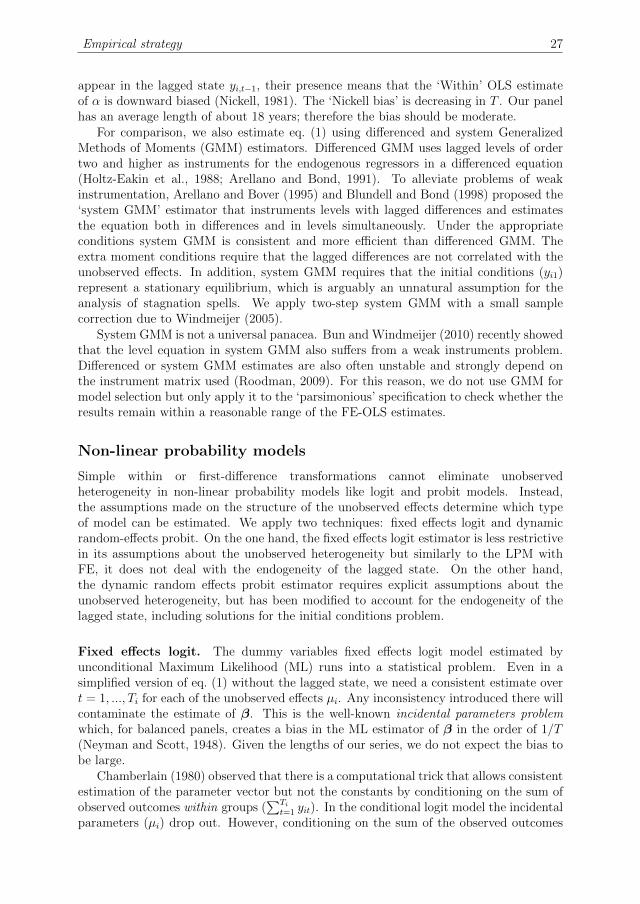
Empirical strategy 27
appear in the lagged state yi,t−1, their presence means that the ‘Within’ OLS estimateof α is downward biased (Nickell, 1981). The ‘Nickell bias’ is decreasing in T . Our panelhas an average length of about 18 years; therefore the bias should be moderate.
For comparison, we also estimate eq. (1) using differenced and system GeneralizedMethods of Moments (GMM) estimators. Differenced GMM uses lagged levels of ordertwo and higher as instruments for the endogenous regressors in a differenced equation(Holtz-Eakin et al., 1988; Arellano and Bond, 1991). To alleviate problems of weakinstrumentation, Arellano and Bover (1995) and Blundell and Bond (1998) proposed the‘system GMM’ estimator that instruments levels with lagged differences and estimatesthe equation both in differences and in levels simultaneously. Under the appropriateconditions system GMM is consistent and more efficient than differenced GMM. Theextra moment conditions require that the lagged differences are not correlated with theunobserved effects. In addition, system GMM requires that the initial conditions (yi1)represent a stationary equilibrium, which is arguably an unnatural assumption for theanalysis of stagnation spells. We apply two-step system GMM with a small samplecorrection due to Windmeijer (2005).
System GMM is not a universal panacea. Bun and Windmeijer (2010) recently showedthat the level equation in system GMM also suffers from a weak instruments problem.Differenced or system GMM estimates are also often unstable and strongly depend onthe instrument matrix used (Roodman, 2009). For this reason, we do not use GMM formodel selection but only apply it to the ‘parsimonious’ specification to check whether theresults remain within a reasonable range of the FE-OLS estimates.
Non-linear probability models
Simple within or first-difference transformations cannot eliminate unobservedheterogeneity in non-linear probability models like logit and probit models. Instead,the assumptions made on the structure of the unobserved effects determine which typeof model can be estimated. We apply two techniques: fixed effects logit and dynamicrandom-effects probit. On the one hand, the fixed effects logit estimator is less restrictivein its assumptions about the unobserved heterogeneity but similarly to the LPM withFE, it does not deal with the endogeneity of the lagged state. On the other hand,the dynamic random effects probit estimator requires explicit assumptions about theunobserved heterogeneity, but has been modified to account for the endogeneity of thelagged state, including solutions for the initial conditions problem.
Fixed effects logit. The dummy variables fixed effects logit model estimated byunconditional Maximum Likelihood (ML) runs into a statistical problem. Even in asimplified version of eq. (1) without the lagged state, we need a consistent estimate overt = 1, ..., Ti for each of the unobserved effects µi. Any inconsistency introduced there willcontaminate the estimate of β. This is the well-known incidental parameters problemwhich, for balanced panels, creates a bias in the ML estimator of β in the order of 1/T(Neyman and Scott, 1948). Given the lengths of our series, we do not expect the bias tobe large.
Chamberlain (1980) observed that there is a computational trick that allows consistentestimation of the parameter vector but not the constants by conditioning on the sum ofobserved outcomes within groups (
∑Tit=1 yit). In the conditional logit model the incidental
parameters (µi) drop out. However, conditioning on the sum of the observed outcomes

28 Chapter 2. The dynamics of stagnation
comes at a cost. Since groups in which yit does not change over Ti provide no informationfor the likelihood, they drop out of the log-likelihood. If there is strong persistence thenumber of observations used in the estimation may fall a lot. Likewise, time-invarianteffects cancel out of the estimation equation. They cannot be estimated, neither canpartial effects since these depend on the expected value of the unobserved effects.
Given the expectation that the unconditional ML estimator is not too strongly biasedand allows estimation of partial effects, we estimate both models and compare theirresults.
Dynamic random effects probit. Conditioning on the sum of the observed outcomesdoes not work for the equivalent probit model. Furthermore, the standard random effectsprobit model assumes that the unobserved heterogeneity is strictly unrelated to theexplanatory variables. The presence of the lagged state (yi,t−1) together with µi violatesthis assumption even if α is actually zero (Wooldridge, 2010, p. 626). This is the problemof true versus spurious state dependence. The estimated effect of yi,t−1 depends on threesources: (1) serial correlation in the errors, (2) correlation with the unobserved effects,and (3) true state dependence (Greene, 2011, p. 769). In such a setting, the ordinary fixedor random effects estimation techniques do not provide consistent estimates. In addition,the outcome path may be severely influenced by the initial conditions (yi1), which enterthe unconditional likelihood function and prohibit integrating out the unobserved effects(µi). We are faced with two related problems: the violation of strict exogeneity in thepresence of unobserved heterogeneity, and the treatment of the initial condition in thelog-likelihood.
A relaxation of the strict exogeneity assumption known as correlated random effectshas been developed for static models following the ideas of Mundlak (1978) andChamberlain (1984). The approach allows for correlation between xit and µi but restrictsthe unobserved effects to depend on means (or other values) of the explanatory variablesaccording to µi = η0 + x′iη2 + εi, where the εi are assumed to be i.i.d. and normallydistributed. The vector xi consists of time-averages (or other values, like initial levels) ofthe regressors xit.
9 While this approach relaxes the strict exogeneity assumption, it doesnot address the issue of dynamics and the related initial conditions problem.
Several solutions to the initial conditions problem have been proposed (see Heckman,1981; Orme, 2001; Wooldridge, 2005). Wooldridge (2005) suggests to condition thedensity (yi1, ..., yiTi) on the observed history of the covariates and the initial values byspecifying a distribution of the unobserved effects given the initial conditions. Rabe-Hesketh and Skrondal (2013) show that this simple method performs well in general andAkay (2012) provides Monte Carlo evidence that a constrained model (with time-averages)also works well in unbalanced panels as long the time series lengths are moderately large.
Concretely, Wooldridge (2005) proposes to condition on the entire time series of thestrictly exogenous variables less the initial period plus the initial condition (yi1) – anapproach that easily extends to interactions. A convenient way to specify the conditionaldistribution of the unobserved effects is µi|yi1, xi ∼ N (η0 + η1yi1 + x′iη2 + x′iyi1η3, σ
2ε),
where xi are the time-averages as in Mundlak-Chamberlain. This implies the followingparametric specification for the unobserved effects: µi = η0 + η1yi1 + x′iη2 + x′iyi1η3 + εi,where the εi are normal, i.i.d., and independent of (yi1, xi).
9Further, this model implies Corr(εi + νit, εi + νis) = σ2ε/(σ
2ε + σ2
ν) for any t 6= s.
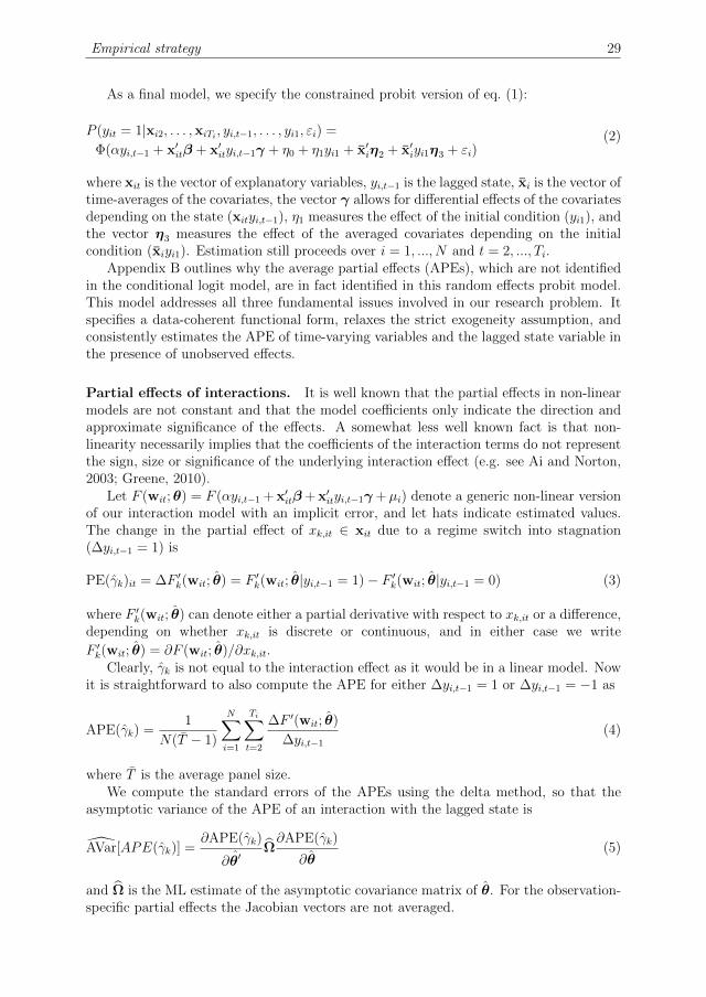
Empirical strategy 29
As a final model, we specify the constrained probit version of eq. (1):
(2)P (yit = 1|xi2, . . . ,xiTi , yi,t−1, . . . , yi1, εi) =
Φ(αyi,t−1 + x′itβ + x′ityi,t−1γ + η0 + η1yi1 + x′iη2 + x′iyi1η3 + εi)
where xit is the vector of explanatory variables, yi,t−1 is the lagged state, xi is the vector oftime-averages of the covariates, the vector γ allows for differential effects of the covariatesdepending on the state (xityi,t−1), η1 measures the effect of the initial condition (yi1), andthe vector η3 measures the effect of the averaged covariates depending on the initialcondition (xiyi1). Estimation still proceeds over i = 1, ..., N and t = 2, ..., Ti.
Appendix B outlines why the average partial effects (APEs), which are not identifiedin the conditional logit model, are in fact identified in this random effects probit model.This model addresses all three fundamental issues involved in our research problem. Itspecifies a data-coherent functional form, relaxes the strict exogeneity assumption, andconsistently estimates the APE of time-varying variables and the lagged state variable inthe presence of unobserved effects.
Partial effects of interactions. It is well known that the partial effects in non-linearmodels are not constant and that the model coefficients only indicate the direction andapproximate significance of the effects. A somewhat less well known fact is that non-linearity necessarily implies that the coefficients of the interaction terms do not representthe sign, size or significance of the underlying interaction effect (e.g. see Ai and Norton,2003; Greene, 2010).
Let F (wit;θ) = F (αyi,t−1 + x′itβ + x′ityi,t−1γ +µi) denote a generic non-linear versionof our interaction model with an implicit error, and let hats indicate estimated values.The change in the partial effect of xk,it ∈ xit due to a regime switch into stagnation(∆yi,t−1 = 1) is
PE(γk)it = ∆F ′k(wit; θ) = F ′k(wit; θ|yi,t−1 = 1)− F ′k(wit; θ|yi,t−1 = 0) (3)
where F ′k(wit; θ) can denote either a partial derivative with respect to xk,it or a difference,depending on whether xk,it is discrete or continuous, and in either case we write
F ′k(wit; θ) = ∂F (wit; θ)/∂xk,it.Clearly, γk is not equal to the interaction effect as it would be in a linear model. Now
it is straightforward to also compute the APE for either ∆yi,t−1 = 1 or ∆yi,t−1 = −1 as
APE(γk) =1
N(T − 1)
N∑
i=1
Ti∑
t=2
∆F ′(wit; θ)
∆yi,t−1
(4)
where T is the average panel size.We compute the standard errors of the APEs using the delta method, so that the
asymptotic variance of the APE of an interaction with the lagged state is
AVar[APE(γk)] =∂APE(γk)
∂θ′Ω∂APE(γk)
∂θ(5)
and Ω is the ML estimate of the asymptotic covariance matrix of θ. For the observation-specific partial effects the Jacobian vectors are not averaged.

30 Chapter 2. The dynamics of stagnation
6 Results and discussion
Linear models. Table 3 reports the results from variations of the LPM. Since weprimarily use the linear models for variable selection, we only briefly discuss the resultsand defer the economic interpretation until the description of the preferred specificationin the next subsection. Column (1) is the standard fixed effects model with standarderrors clustered at the country level. Column (2) is similar but allows for arbitraryheteroskedasticity and autocorrelation within both country and time clusters (Cameron,Gelbach, and Miller, 2011). Column (3) shows the FGLS estimator with clustering atthe country level via the weights. Column (4) is the parsimonious FGLS specificationdiscarding those interaction terms that are individually and jointly insignificant. Columns(5) and (6) re-estimate (4) using system GMM.
Two joint hypothesis tests reported in Table 3 are key to our model-building approach.First, we test if the coefficients of the interactions with the lagged state and the coefficientof the lagged state are jointly zero; taken together these variables comprise Set I. In allmodels this hypothesis is rejected, indicating the presence of dynamics. Second, we testwhether the interactions with the lagged state that are individually insignificant at the10% level (i.e., Set II) can also be jointly omitted. In columns (1) to (4), the insignificantinteractions pass this joint-exclusion test, but not in the GMM estimates.
All fully-interacted specifications provide very similar results. Inflation, financialopenness, trade openness, and negative regime changes clearly affect the probability ofentering a stagnation spell. Considering the interactions, the coefficients of inflation, tradeopenness, and negative regime changes are significant in most but not all specifications.Interestingly, the interaction terms often have the opposite sign of the non-interactedcoefficients, indicating that the respective effects are weaker within a stagnation spell.Column (4) only retains the significant interactions and represents our parsimoniousspecification which we later re-estimate with non-linear techniques. We still find evidencethat inflation, trade openness, and negative regime changes have a different impact withinthe spell than on the onset probabilities. However, the interaction effect of financialopenness is, again, insignificant.
The system GMM specifications in columns (5) and (6) assess the stability of theparameter estimates once we account for the endogeneity of the lagged state and theinteractions with the lagged state. While the significance of individual coefficientschanges between the two GMM models, the sizes and signs of the previously highlightedcoefficients remain broadly similar. In column (5) we use the second and third lag ofthe predetermined variables as instruments. Nevertheless, the J-test indicates that thenumber of instruments is too large relative to the group size. We address this concern incolumn (6) by collapsing the instrument set (see Roodman, 2009). There is no evidenceof instrument endogeneity and the estimated parameters come closer to the earlier least-squares estimates. However, applying GMM in our context is not ideal. A moderateT quickly leads to instrument proliferation and problems in identifying an instrumentset that balances efficiency gains with decreasing relevance. Accordingly, we place lessemphasis on the GMM results and rely more on verifying the results from the precedinglinear models with non-linear techniques.
The linear models point to several preliminary conclusions. First, we find thatinflation, financial openness, trade openness, and negative regime changes have astatistically significant effect on the probability of stagnation, and so do to a lesser extentexchange rate undervaluation and inequality. Second, state dependence plays a large

Results and discussion 31
Table
3–
Lin
ear
Mod
els
–P
rob
abil
ity
ofS
tagn
atio
n
(1)
(2)
(3)
(4)
(5)
(6)
Ind
epen
den
tV
ari
ab
leL
PM
S.E
.L
PM
S.E
.F
GL
SS
.E.
FG
LS
S.E
.S
YS
-GM
MS
.E.
SY
S-G
MM
S.E
.
Log
GD
PC
(t−1)
0.0
52
0.0
73
0.0
52
0.0
94
0.0
61
0.0
73
0.0
40
0.0
65
-0.0
18
0.0
35
-0.0
29
0.0
20
Infl
ati
on(t−1)
0.0
05*
0.0
03
0.0
05
0.0
04
0.0
05**
0.0
02
0.0
05**
0.0
02
0.0
03
0.0
04
0.0
13
0.0
10
∆T
oT
(t−1)
-0.0
80
0.0
81
-0.0
80
0.0
82
-0.0
92
0.1
09
-0.0
36
0.0
54
-0.0
35
0.0
43
-0.0
56
0.0
49
∆R
eal
Exp
ort
s (t−
1)
-0.1
36
0.1
69
-0.1
36
0.1
77
-0.0
80
0.1
43
-0.0
14
0.0
47
0.0
11
0.0
67
0.0
55
0.0
62
RE
RV
alu
e (t−
1)
-0.1
50*
0.0
88
-0.1
50
0.1
13
-0.0
83
0.0
75
-0.0
16
0.0
39
-0.1
46***
0.0
46
-0.1
55***
0.0
42
Fin
.O
pen
nes
s (t−
1)
-0.0
43***
0.0
16
-0.0
43**
0.0
20
-0.0
42**
0.0
17
-0.0
34**
0.0
16
-0.0
43*
0.0
23
-0.0
20
0.0
26
Tra
de
Op
enn
ess (t−
1)
-0.2
36***
0.0
81
-0.2
36***
0.0
73
-0.2
33***
0.0
62
-0.2
31***
0.0
58
-0.1
85
0.1
48
-0.2
86**
0.1
25
Ineq
uali
ty(t−1)
-0.0
07
0.0
04
-0.0
07
0.0
05
-0.0
03
0.0
04
-0.0
02
0.0
03
0.0
07**
0.0
03
0.0
05**
0.0
02
Poli
ty2(t−1)
-0.0
11
0.0
07
-0.0
11
0.0
07
-0.0
08*
0.0
05
-0.0
03
0.0
03
-0.0
03
0.0
04
-0.0
04
0.0
04
Reg
chan
ge
+(t−1)
0.0
33
0.0
68
0.0
33
0.0
77
0.0
06
0.1
03
0.0
17
0.0
32
0.0
36
0.0
36
0.0
31
0.0
43
Reg
chan
ge−
(t−1)
0.3
38*
0.1
87
0.3
38
0.2
02
0.2
77*
0.1
49
0.2
74*
0.1
43
0.4
50
1.0
50
0.3
48*
0.2
10
Lea
der
Exit(t−1)
-0.0
71
0.0
53
-0.0
71
0.0
55
-0.0
45
0.0
54
0.0
04
0.0
28
-0.0
37
0.0
43
-0.0
33
0.0
43
War/
Con
flic
t (t−
1)
0.0
83
0.0
65
0.0
83
0.0
91
0.0
97
0.0
87
-0.0
05
0.0
42
-0.0
22
0.0
68
0.0
16
0.0
80
Log
GD
PC
(t−1)×y(t−1)
0.0
02
0.0
48
0.0
02
0.0
50
-0.0
39
0.0
42
Infl
ati
on(t−1)×y(t−1)
-0.0
04*
0.0
03
-0.0
04
0.0
04
-0.0
05**
0.0
02
-0.0
05**
0.0
02
-0.0
02
0.0
04
-0.0
12
0.0
10
∆T
oT
(t−1)×y(t−1)
0.0
31
0.0
93
0.0
31
0.0
84
0.0
67
0.1
25
∆R
eal
Exp
ort
s (t−
1)×y(t−1)
0.1
17
0.1
66
0.1
17
0.1
69
0.0
73
0.1
51
RE
RV
alu
e (t−
1)×y(t−1)
0.1
46
0.1
03
0.1
46
0.1
05
0.0
81
0.0
75
Fin
.O
pen
nes
s (t−
1)×y(t−1)
0.0
21
0.0
19
0.0
21
0.0
19
0.0
34*
0.0
18
0.0
23
0.0
16
0.0
64**
0.0
29
0.0
38
0.0
39
Tra
de
Op
enn
ess (t−
1)×y(t−1)
0.1
86**
0.0
84
0.1
86**
0.0
88
0.2
07***
0.0
66
0.2
08***
0.0
59
0.1
32
0.1
69
0.2
92*
0.1
48
Ineq
uali
ty(t−1)×y(t−1)
0.0
01
0.0
03
0.0
01
0.0
04
0.0
01
0.0
03
Poli
ty2(t−1)×y(t−1)
0.0
07
0.0
07
0.0
07
0.0
07
0.0
07
0.0
05
Reg
chan
ge
+(t−1)×y(t−1)
-0.0
17
0.0
68
-0.0
17
0.0
76
0.0
11
0.1
08
Reg
chan
ge−
(t−1)×y(t−1)
-0.3
54*
0.1
84
-0.3
54*
0.1
93
-0.2
80*
0.1
66
-0.2
77*
0.1
60
-0.3
99
1.0
40
-0.3
63*
0.2
11
Lea
der
Exit(t−1)×y(t−1)
0.1
01*
0.0
60
0.1
01
0.0
68
0.0
59
0.0
60
War/
Con
flic
t (t−
1)×y(t−1)
-0.1
71**
0.0
81
-0.1
71*
0.0
90
-0.1
26
0.0
96
y(t−1)
0.1
58
0.4
73
0.1
58
0.5
05
0.4
86
0.4
23
0.2
22***
0.0
59
0.3
63**
0.1
60
0.3
17**
0.1
41
Con
stant
0.7
58
0.7
46
0.3
73
0.8
46
0.4
63
0.6
47
0.6
17
0.5
60
0.3
68
0.3
92
0.5
08*
0.2
61
Ob
serv
ati
on
s1691
1691
1691
1691
1691
1691
Cou
ntr
yF
EY
esY
esY
esY
es–
–C
lust
ers
cou
ntr
yco
untr
y+
yea
rco
untr
yco
untr
yco
untr
yco
untr
yJoin
t:C
ou
ntr
yF
E[p
-valu
es]
0.0
00
0.0
00
0.0
00
0.0
00
Join
t:5-Y
ear
FE
[p-v
alu
es]
0.1
01
0.4
51
0.4
30
0.3
64
0.0
53
0.0
24
Join
t:S
etI
[p-v
alu
es]
0.0
00
0.0
00
0.0
00
0.0
00
0.0
00
0.0
00
Join
t:S
etII
[p-v
alu
es]
0.7
96
0.2
26
0.7
08
0.1
67
0.7
59
0.0
38
Inst
rum
ents
390
35
AR
1[p
-valu
e]0.0
00
0.0
00
AR
2[p
-valu
e]0.3
04
0.1
20
Han
sen
’sJ
[p-v
alu
e]1.0
00
0.3
27
Note
s:∗∗∗ p<
0.01,∗∗p<
0.05,∗p<
0.1.

32 Chapter 2. The dynamics of stagnation
role in determining whether a country experiences a stagnation episode or not. Third,in all specifications there is considerable evidence of unobserved heterogeneity at thecountry level. Fourth, all significant interaction terms with the lagged state point intothe direction opposite of their linear counterparts.
Non-linear models. Turning to the non-linear models, we first discuss theheterogeneity of the interaction effects using a logit specification and then present theresults from the dynamic random effects probit estimator (our preferred specification).
Table 4 shows the estimation results from two types of fixed effects logit estimators.As a reference, column (1) shows the fully interacted model estimated using conditionalmaximum likelihood, where the fixed effects are not estimated but drop out. Column (2)is the conditional logit equivalent of the parsimonious linear model, and column (3a) isthe same model using dummy variables for the country fixed effects. The last column(3b) reports the APEs based on column (3a). The APEs of interaction terms are reportedsimilarly to coefficients of a linear model; that is, if yi,t−1 = 0, the APE is reported in therow of the non-interacted variable and, for yi,t−1 = 1, the total APE is the sum of theformer and the APE of the interaction term.
A complication in interpreting the results of the conditional logit models is that theAPEs are not identified, for the simple reason that the individual country effects arenot estimated. In order to approximate the APEs, we estimate the equivalent dummyvariables fixed effects logit model and compute the APEs based on its results. Columns(2) and (3a) show that the parameter estimates and the corresponding standard errorsremain very similar, justifying this approach.
We still find evidence that inflation, financial openness, trade liberalization, andnegative regime changes significantly affect the probability of stagnation. However,for all but negative regime changes, the APEs of the interaction terms are statisticallyinsignificant and, in the case of financial openness, the interaction effect no longer pointsin the opposite direction. Applying fixed effects logit also substantially reduces theestimation sample to 1314 observations in 62 countries, for lack of within-group variation.This loss of observations makes it impossible to identify the effect of the negative regimechange interaction term; as a consequence, the interaction is dropped from the earlierparsimonious model.
The APEs are close to the linear approximation in terms of size. Notable changesare that now the effects of changes in the terms of trade, real exchange rate (RER)undervaluation, and inequality are all significant at the 10% level and have increasedsubstantially in absolute size. The degree of state dependence identified by the logitmodel is also somewhat higher than in the linear approximation (a 32.1 percentage pointshigher probability of continuation if a country was stagnating the year before).
Table 4 may seem to provide little evidence that some variables have a different impacton the onset of a stagnation spell than on its continuation. However, in non-linear models,the partial effects of the interaction can be very heterogeneous at the observation leveland may be individually significant for a substantial subset of observations. By definition,APEs ‘average out’ this type of heterogeneity which can be especially troublesome if thepartial effects switch signs. In Figure 2 we examine these non-linearities more closely.The figure graphs the distributions of partial effects for the interaction terms of inflation,financial openness, and trade openness over the predicted probability of stagnation, aswell as the associated p-values of a Wald-test of the null that the interaction effect ateach particular observation is zero.

Results and discussion 33
Table 4 – Logit Models – Probability of Stagnation
(1) (2) (3a) (3b)Independent Variable Logit CML S.E. Logit CML S.E. Logit ML S.E. APEs S.E.
Log GDPC(t−1) 0.417 0.707 0.430 0.695 0.430 0.738 0.058 0.099Inflation(t−1) 0.037 0.025 0.043 0.026 0.046 0.028 0.006* 0.004∆ ToT(t−1) -0.556 0.571 -0.828* 0.479 -0.885* 0.516 -0.119* 0.070∆ Real Exports(t−1) -0.784 1.163 -0.621 0.735 -0.681 0.795 -0.091 0.107RER Value(t−1) -1.375** 0.567 -0.957* 0.503 -1.020* 0.533 -0.137* 0.071Fin. Openness(t−1) -0.453*** 0.121 -0.396*** 0.110 -0.421*** 0.118 -0.058*** 0.016Trade Openness(t−1) -1.441*** 0.486 -1.424*** 0.456 -1.527*** 0.489 -0.259*** 0.091Inequality(t−1) -0.050 0.031 -0.052* 0.029 -0.054* 0.030 -0.007* 0.004Polity2(t−1) -0.066 0.044 -0.051 0.033 -0.054 0.036 -0.007 0.005Regchange +(t−1) 0.193 0.561 0.129 0.376 0.136 0.397 0.018 0.054Regchange −(t−1) 2.102** 0.900 1.945** 0.938 2.038** 0.991 0.288** 0.135Leader Exit(t−1) -0.501 0.426 -0.060 0.317 -0.058 0.334 -0.007 0.044War/Conflict(t−1) 0.115 0.382 -0.428 0.342 -0.454 0.357 -0.059 0.045Log GDPC(t−1) × y(t−1) 0.082 0.284Inflation(t−1) × y(t−1) -0.012 0.012 -0.019 0.015 -0.021 0.016 -0.002 0.002∆ ToT(t−1) × y(t−1) -1.128 1.025∆ Real Exports(t−1) × y(t−1) 0.290 1.244RER Value(t−1) × y(t−1) 0.859 0.624Fin. Openness(t−1) × y(t−1) 0.144 0.117 0.045 0.107 0.045 0.116 -0.011 0.022Trade Openness(t−1) × y(t−1) 0.947* 0.528 0.885* 0.487 0.939* 0.521 0.153 0.094Inequality(t−1) × y(t−1) 0.003 0.019Polity2(t−1) × y(t−1) 0.013 0.042Regchange +(t−1) × y(t−1) -0.164 0.620Leader Exit(t−1) × y(t−1) 0.833* 0.506War/Conflict(t−1) × y(t−1) -1.051* 0.537y(t−1) -0.004 2.813 1.189*** 0.456 1.282*** 0.487 0.321*** 0.029
Observations 1314 1314 1314Country FE Yes Yes Yes5 Year FE Yes Yes YesClustered Errors [Country] Yes Yes YesCountries 62 62 62Log-pseudolikelihood -465.864 -469.311 -555.547
Notes: In column (1) Regchange −(t−1) × y(t−1) had been dropped due to a lack of within-groupvariance. The asymptotic standard errors of the APEs are computed via the delta method.∗∗∗p < 0.01,∗∗ p < 0.05,∗ p < 0.1.
Clearly, the partial effects of all three interaction terms are extremely non-linearand tend to include both positive and negative values. In the case of inflation, we findthat for some observations the partial effect is positive, while for most observations itis negative and insignificant. The effect is significant only at negative values for a verysmall fraction of the distribution (30 observations) and ranges from −0.95% to 0.39%,which is moderately large compared to an APE of 0.6% when yi,t−1 = 0. The predictedpartial effects group into two families of curves with an S-shape. The curves at lowerstagnation probabilities are the partial effects for observations where yi,t−1 = 0 (symbol:o) and the curves going across higher stagnation probabilities are the predicted effectsfor observations where yi,t−1 = 1 (symbol: x). The dashed line refers to the APE in theupper panel and the p-value of a Wald test that the APE is zero in the lower panel.
The interaction effect for financial openness is also S-shaped but sloping upwards andranges from −6.9% to 7.6%. The partial effect is statistically significant for 14% of thepredicted outcomes at both negative and positive values. However, similarly to inflation,the large range of insignificant negative and positive values supports the conclusion thatthe effect is not different from zero on average. In contrast, the evidence of a significantinteraction is relatively strong for trade openness. For most observations the partial effect

34 Chapter 2. The dynamics of stagnation
Figure 2 – Partial Effects of Interaction Terms in Logit Model
−.01
−.005
0
.005
Part
ial E
ffect
0 .2 .4 .6 .8 1Predicted Probability
yi,t−1=1 yi,t−1=0
Inflation
−.01
−.005
0
.005
Part
ial E
ffect
0 .2 .4 .6 .8 1p−value
yi,t−1=1 yi,t−1=0
−.1
−.05
0
.05
.1
Part
ial E
ffect
0 .2 .4 .6 .8 1Predicted Probability
yi,t−1=1 yi,t−1=0
Fin. Openness
−.1
−.05
0
.05
.1
Part
ial E
ffect
0 .2 .4 .6 .8 1p−value
yi,t−1=1 yi,t−1=0
0
.1
.2
.3
Part
ial E
ffect
0 .2 .4 .6 .8 1Predicted Probability
yi,t−1=1 yi,t−1=0
Trade Openness
0
.1
.2
.3
Part
ial E
ffect
0 .2 .4 .6 .8 1p−value
yi,t−1=1 yi,t−1=0
Notes: The dashed line refers to the APE in the upper panel and the p-value of a Wald test thatthe APE is zero in the lower panel.“Predicted Probability” is the probability of stagnationP (yit = 1).
of the interaction term is positive and very large, with an overall range from −3% to 30%.For about 32% of the observations in the sample the partial effect of the interaction termis individually significant at the 5% level.
Overall, the logit specifications confirm the findings of the linear models given a fewrefinements. Inflation, financial openness, trade openness, and negative regime changesremain significant predictors of being in stagnation. Furthermore, these estimates suggestthat exchange rate undervaluation, changes in the terms of trade, and inequality affectthe probability of stagnation. However, the evidence in favor of interaction effects withthe lagged state for any other variable than trade openness is weak; the estimates suggestthat only trade openness has a different impact on the onset of a stagnation spell thanits continuation.
We now turn to the last and final set of estimates. Table 5 presents the randomeffects probit estimates of the dynamic panel model. For comparison purposes, we firstreport the naıve pooled probit version of the fully-interacted dynamic model and then itsrandom effects counterpart estimated according to the Wooldridge approach – columns(1) and (2), respectively. Column (3a) is parsimonious version of the dynamic randomeffects model in column (2) and our preferred specification. Column (3b) reports theAPEs of the variables of interest and their associated standard errors.
We report several additional rows in Table 5 to display the regression results more

Results and discussion 35
Table 5 – Probit Models – Probability of Stagnation
(1) (2) (3a) (3b)Independent Variable Probit S.E. Woold S.E. Woold S.E. APEs S.E.
Log GDPC(t−1) 0.027 0.103 0.449 0.377 0.398 0.367 0.083 0.076Inflation(t−1) 0.017*** 0.006 0.012 0.008 0.020*** 0.008 0.005*** 0.002∆ ToT(t−1) -0.328 0.300 -0.435 0.476 -0.321 0.349 -0.067 0.072∆ Real Exports(t−1) -0.226 0.540 -0.570 0.565 -0.362 0.358 -0.075 0.074RER Value(t−1) -0.719*** 0.202 -0.786** 0.331 -0.513* 0.278 -0.106* 0.058Fin. Openness(t−1) -0.056 0.039 -0.205*** 0.074 -0.153** 0.073 -0.038** 0.018Trade Openness(t−1) -0.567*** 0.217 -0.926*** 0.240 -0.774*** 0.228 -0.218*** 0.068Inequality(t−1) 0.014** 0.007 -0.026 0.016 -0.022 0.015 -0.004 0.003Polity2(t−1) -0.014 0.013 -0.031 0.020 -0.027* 0.016 -0.006* 0.003Regchange +(t−1) 0.039 0.269 0.138 0.405 0.066 0.220 0.014 0.046Regchange −(t−1) 1.074* 0.557 1.238** 0.617 1.047* 0.584 0.214* 0.112Leader Exit(t−1) -0.196 0.188 -0.118 0.235 -0.006 0.171 -0.001 0.035War/Conflict(t−1) 0.110 0.257 0.280 0.374 -0.199 0.246 -0.041 0.051Log GDPC(t−1) × y(t−1) -0.259 0.182 -0.129 0.154Inflation(t−1) × y(t−1) -0.008 0.006 -0.004 0.008 -0.012 0.008 -0.003 0.002∆ ToT(t−1) × y(t−1) -0.091 0.393 -0.097 0.750∆ Real Exports(t−1) × y(t−1) -0.435 0.574 0.286 0.745RER Value(t−1) × y(t−1) 0.635 0.390 0.532* 0.308Fin. Openness(t−1) × y(t−1) 0.096 0.060 0.086 0.078 -0.019 0.068 -0.006 0.017Trade Openness(t−1) × y(t−1) 0.474 0.321 0.816*** 0.262 0.646*** 0.238 0.186*** 0.067Inequality(t−1) × y(t−1) 0.005 0.012 0.008 0.011Polity2(t−1) × y(t−1) 0.008 0.022 0.005 0.020Regchange +(t−1) × y(t−1) 0.166 0.284 -0.137 0.482Leader Exit(t−1) × y(t−1) 0.290 0.259 0.201 0.290War/Conflict(t−1) × y(t−1) -0.267 0.404 -0.803* 0.458y0 0.969 2.621 1.244*** 0.477y(t−1) 3.407* 1.787 1.554 1.569 1.020*** 0.229 0.389*** 0.035Constant -1.287 1.105 -0.733 2.482 -2.958 1.871
Observations 1586 1471 1596η2-estimated? NO YES YESη3-estimated? NO YES YES5-Year FE YES YES YESCountries 90 81 90Pseudo-R2 0.423 0.269 0.255Log-likelihood -632.218 -574.211 -596.272
Notes: In column (1) Regchange −(t−1) × y(t−1) had been dropped due to a lack of within-groupvariance. The asymptotic standard errors of the APEs are computed via the delta method.∗∗∗p < 0.01,∗∗ p < 0.05,∗ p < 0.1.
succinctly. The row “η2-estimated?” refers to whether the Mundlak-Chamberlain time-averages are included. As these are not interesting by themselves, we do not report theircoefficients and partial effects. Similarly, the row “η3-estimated?” reports whether theinteraction terms are included twice, once as an interaction with the lagged state andonce as an interaction with the initial condition. We also do not report the parameterestimates of the latter, as they primarily account for the non-random nature of theunobserved effects.
The random effects probit model gives different (and superior) estimates comparedto the pooled probit version.10 Several parameters exhibit sign changes and substantialchanges in significance levels. More interestingly, even though the Wooldridge estimatorof the dynamic model includes several additional terms and requires the assumptionthat the regressors are only correlated with the unobserved heterogeneity through their
10The coefficients are scaled differently. The comparison should be done in terms of relative sizes,signs, and significance levels – where appropriate.

36 Chapter 2. The dynamics of stagnation
averages, the results are remarkably similar to those of the linear models (in Table 3) andlogit specifications (in Table 4). We do not compute the partial effects at the observation-level as only the APEs across the entire distribution of the unobserved heterogeneity areidentified (see Appendix B and Wooldridge, 2005).
The APE of inflation is similar to that in the previous models. According to theWooldridge estimator, a unit increase in the inflation index in t − 1 translates into 0.5percentage points higher probability of stagnation in year t, if the country was not instagnation in t − 1. The APE of the interaction effect is −0.3% and insignificant at allconventional levels, supporting the view that inflation increases the chances of stagnation,no matter if this occurs within or outside of a stagnation spell. We find no evidence infavor of the hypothesis that (higher) inflation helps exiting a stagnation spell.
Next, the effect of financial openness is also similar to that estimated by the linearprobability model. A unit increase in the Chinn-Ito index towards more openness reducesthe probability of stagnation by 3.8 percentage points. The APE of the interaction term issmall and insignificant (−0.6%), suggesting that there is no difference between onset andcontinuation probabilities. This result is particularly interesting, since capital accountopenness is sometimes restricted during crises to avert capital flight. Yet we find noevidence that it increases the risk of stagnation when a country is already stagnating,but instead it seems to be associated with a lower probability of crisis throughout.
In the case of trade openness, a discrete change towards openness when yi,t−1 = 0has an average partial effect of −21.8%, which is similar to the previous results. Theinteraction term is highly significant and has a very large effect on the predictedprobability of stagnation (18.6%). Adding these two effects, we get the APE for theprobability of continued stagnation if yi,t−1 = 1 and the country is open to trade whichis still negative but statistically insignificant (−3.2%). Trade openness has alreadybeen shown to affect growth rates (Wacziarg and Welch, 2008), growth accelerations(Hausmann et al., 2005), and the duration of positive growth spells (Berg et al., 2012).Our results add that open economies are significantly less likely to fall into a stagnationspell – it is the single largest effect of a non-political variable in all specifications – butalso that openness does not significantly improve the chances of exiting a stagnation spell.
This finding suggests that, on top of typically being linked to higher average growthrates, trade openness is ‘good for growth’ in the sense that it protects countries fromstagnation. While trade benefits growth through specialization, technological diffusion,and higher investment levels, it can also stabilize and accelerate growth but it doesnot necessarily lead to shorter crises (especially when these are caused by internationalfactors). Arguably, the weaker within-stagnation effect could also be driven by the factthat countries often liberalize in response to an ongoing crisis which often yields noimmediate benefits and can temporarily increase volatility (Wacziarg and Welch, 2008).
Regarding the political shocks, the confidence interval of the APE of negative regimechanges widens a bit (the t-statistic is 1.90), but the absolute size of the effect remainslarge. If a country experiences a negative regime change, then the probability ofstagnation increases by 21.4 percentage points. As in the logit models, we could notinclude the interaction term due to a lack of time variation. Whereas negative regimechanges were previously linked to the onset of growth accelerations (Hausmann et al.,2005), our analysis reveals the more plausible result that they strongly predict stagnationepisodes. None of the other political variables, that is positive regime changes, irregularleader exits or the Polity score, are robustly related with the incidence of stagnationspells. This finding stands in sharp contrast to the ‘institutions trump other factors’

Results and discussion 37
perspective (e.g. Acemoglu et al., 2001, 2002; Rodrik et al., 2004) but could be drivenby our focus on annual transitions in and out of crises (which are likely to be caused bymore proximate factors). Aidt and Gassebner (2010), for example, find that the level oftrade integration is endogenous to the political regime. Autocratic countries trade lessthan democracies, but steps towards improving the accountability of leaders can lead tohigher trade integration in the medium-run.
Undervaluation of the real exchange rate has a moderate and marginally significanteffect on the probability of stagnation. A one standard deviation change in theundervaluation index reduces the probability of both the onset and continuation ofstagnation by about 4%. We cannot corroborate the results from the logit model thatchanges in the terms of trade and inequality have any meaningful effect on the probabilityof stagnation. In addition, wars, and civil conflict do not predict stagnation spells, andthere is no evidence of an effect of the level of GDP per capita.
Table 5 also reveals that the degree of state dependence is underestimated by boththe LPM and FE logit model. If a country experienced stagnation in the previous year,it is 38.9 percentage points more likely to be in stagnation in the current year. Pathdependence is thus an important feature of the stagnation process. The models also fitthe data reasonably well (Pseudo-R2 = 0.255) and the fit compares favorably to the onsetmodels used elsewhere (e.g. Hausmann et al., 2005, 2008) – although these goodness of fitcriteria are not strictly comparable. Hence, we find that dynamic models a) allow us totest refined hypotheses about the difference between onset and continuation of stagnationspells, and b) lead to better predictions of when stagnation occurs.
To summarize, the main results are robust to different specifications, assumptionsabout the unobserved effects, and correlation between the observed variables andunobserved country-effects. Most of the preferred specifications identify the lags ofinflation and negative regime changes as strong predictors of stagnation episodes. Severalmodels also identify trade openness and financial openness as relevant. The non-linearmodels add three important insights. First, there is less evidence of interaction effectswith the lagged state than the LPM suggests. The interactions are highly non-linearand vary significantly across the sample, but only in the case of trade openness wefind convincing evidence that its effect differs depending on whether the country wasin stagnation before or not. The evidence of interaction effects between the lagged stateand inflation, financial openness, or negative regime changes is weak. Second, the non-linear models show that the real exchange rate matters for stagnation. An overvalued realexchange rate raises the chances of stagnation, while undervaluation reduces it. Third,the level of state dependence is still moderate, but larger than estimated by the linearmodels with fixed effects.
We also find that lagging all included regressors by one year to assure that theyare at least contemporaneously exogenous results in identifying very different factors assignificant than if the issue of endogeneity is left unaddressed. For example Hausmannet al. (2008), who studied the onset of stagnation, found that exports, inflation, wars,and political transitions matter. We do not find significant effects for exports and wars,although we do confirm their results for inflation and negative regime changes.
Interestingly, we cannot confirm two central results of the previous literature. First,we find little evidence that, apart from negative regime changes, institutions generallyaffect the incidence of stagnation. Consistent with the institutionalist literature, we findthat poor countries are more prone to stagnation and crisis, but our analysis contradictsthe hypotheses that weak institutions increase the incidence of stagnation. On the
38 Chapter 2. The dynamics of stagnation
contrary, traditional macroeconomic variables predict the incidence of stagnation ratherwell. Second and contrary to previous research (Rodrik, 1999; Hausmann et al., 2008),our data does not support the finding that changes in real exports or terms of trade affectthe probability of stagnation.
7 Concluding remarks
This chapter provides a dynamic analysis of the incidence of stagnation and examinesif stagnation spells are determined by institutional factors, various shocks, ormacroeconomic factors. Building on a recent contribution by Hausmann et al. (2008), wedefine stagnation spells as episodes in which GDP per capita is below previously achievedlevels. We then use fixed effects linear models, GMM, fixed effects logit, and dynamicrandom effects probit to assess the role of institutions, political shocks, and economicfactors. In contrast to the previous literature, we explicitly examine the hypothesis thatthe effects of variables on the onset of stagnation and on the continuation of stagnationmay be different.
We identify several factors that explain the incidence of stagnation spells. Adverseregime changes have the single largest effect on the incidence of stagnation, while higherinflation increases the chances of being in stagnation. More surprisingly, we find that realexchange rate undervaluation, financial openness, and trade openness help reduce thechances of stagnation. Additionally, we evidence that trade openness primarily protectsagainst falling into stagnation, but does not speed up recovery. For all other variablesthere is no evidence of a differential impact on onset versus continuation.
Though traditional macroeconomic factors have the upper hand in our explanationsof stagnation compared to institutional factors, we do not yet know to what extentmacroeconomic factors are in turn influenced by underlying institutional characteristics.The use of more differentiated measures and time series for institutions as well asadditional techniques for dealing with endogeneity might add further insights. This is apromising avenue for future research.

Bibliography 39
Bibliography
Acemoglu, D., S. Johnson, and J. A. Robinson (2001). The colonial origins of comparative development:An empirical investigation. American Economic Review 91 (5), 1369–1401.
Acemoglu, D., S. Johnson, and J. A. Robinson (2002). Reversal of Fortune: Geography and Institutionsin the Making of the Modern World Income Distribution. Quarterly Journal of Economics 117 (4),1231–1294.
Acemoglu, D., S. Johnson, J. A. Robinson, and Y. Thaicharoen (2003). Institutional causes,macroeconomic symptoms: volatility, crises and growth. Journal of Monetary Economics 50 (1),49–123.
Ai, C. and E. C. Norton (2003). Interaction terms in logit and probit models. Economics Letters 80 (1),123–129.
Aidt, T. S. and M. Gassebner (2010). Do autocratic states trade less? The World Bank EconomicReview 24 (1), 38–76.
Akay, A. (2012). Finite-sample comparison of alternative methods for estimating dynamic panel datamodels. Journal of Applied Econometrics 27 (7), 1189–1204.
Arellano, M. and S. Bond (1991). Some tests of specification for panel data: Monte Carlo evidence andan application to employment equations. Review of Economic Studies 58 (2), 277–297.
Arellano, M. and O. Bover (1995). Another look at the instrumental variable estimation of error-components models. Journal of Econometrics 68 (1), 29–51.
Aron, J. (2000). Growth and institutions: A review of the evidence. World Bank ResearchObserver 15 (1), 99–135.
Barro, R. J. (2000). Inequality and Growth in a Panel of Countries. Journal of Economic Growth 5 (1),5–32.
Berg, A., J. D. Ostry, and J. Zettelmeyer (2012). What makes growth sustained? Journal of DevelopmentEconomics 98 (2), 149–166.
Bluhm, R. and A. Szirmai (2012). Institutions and long-run growth performance: An analytic literaturereview of the institutional determinants of economic growth. UNU-MERIT Working Paper Series033, United Nations University, Maastricht Economic and social Research and training centre onInnovation and Technology.
Blundell, R. and S. Bond (1998). Initial conditions and moment restrictions in dynamic panel datamodels. Journal of Econometrics 87 (1), 115–143.
Bun, M. J. G. and F. Windmeijer (2010). The weak instrument problem of the system GMM estimatorin dynamic panel data models. Econometrics Journal 13 (1), 95–126.
Bussiere, M. and M. Fratzscher (2006). Towards a new early warning system of financial crises. Journalof International Money and Finance 25 (6), 953–973.
Cameron, A. C., J. B. Gelbach, and D. L. Miller (2011). Robust inference with multiway clustering.Journal of Business & Economic Statistics 29 (2), 238–249.
Cerra, V. and S. C. Saxena (2008). Growth dynamics: The myth of economic recovery. AmericanEconomic Review 98 (1), 439–57.
Chamberlain, G. (1980). Analysis of covariance with qualitative data. Review of Economic Studies 47 (1),225–238.
Chamberlain, G. (1984). Panel data. In Z. Griliches and M. D. Intriligator (Eds.), Handbook ofEconometrics, Volume 2 of Handbook of Econometrics, pp. 1247–1318. Elsevier.
Cheibub, J. A., J. Gandhi, and J. R. Vreeland (2010). Democracy and dictatorship revisited. PublicChoice 143 (1/2), 67–101.
Chinn, M. D. and H. Ito (2006). What matters for financial development? Capital controls, institutions,and interactions. Journal of Development Economics 81 (1), 163–192.
Crombrugghe, D. d. and K. Farla (2012). Preliminary conclusions on institutions and economicperformance. UNU-MERIT Working Paper Series 035, United Nations University, MaastrichtEconomic and social Research and training centre on Innovation and Technology.
Deininger, K. and L. Squire (1998). New ways of looking at old issues: inequality and growth. Journalof Development Economics 57 (2), 259–287.
Diebold, F. X., G. Rudebusch, and D. Sichel (1993). Further evidence on business-cycle durationdependence. In J. H. Stock and M. W. Watson (Eds.), Business Cycles, Indicators, and Forecasting,Volume 28 of Studies in Business Cycles, Chapter 6, pp. 255–285. University of Chicago Press.

40 Bibliography
Engerman, S. L. and K. L. Sokoloff (1997). Factor endowments, institutions, and differential growthpaths among new world economies. In S. Haber (Ed.), How Latin America Fell Behind, pp. 260–296.Stanford, CA: Stanford University Press.
Forbes, K. J. (2000). A Reassessment of the Relationship between Inequality and Growth. AmericanEconomic Review 90 (4), 869–887.
Glaeser, E. L., R. La Porta, F. Lopez-de Silanes, and A. Shleifer (2004). Do institutions cause growth?Journal of Economic Growth 9 (3), 271–303.
Gleditsch, N. P., P. Wallensteen, M. Eriksson, M. Sollenberg, and H. Strand (2002). Armed conflict1946-2001: A new dataset. Journal of Peace Research 39 (5), 615–637.
Goemans, H. E., K. S. Gleditsch, and G. Chiozza (2009). Introducing Archigos: A dataset of politicalleaders. Journal of Peace Research 46 (2), 269–283.
Greene, W. H. (2010). Testing hypotheses about interaction terms in nonlinear models. EconomicsLetters 107 (2), 291–296.
Greene, W. H. (2011). Econometric Analysis (7th ed.). Upper Saddle River, NJ: Prentice Hall.
Greif, A. (2006). Institutions and the path to the modern economy: Lessons from medieval trade.Cambridge University Press.
Hall, R. E. and C. I. Jones (1999). Why Do Some Countries Produce So Much More Output Per WorkerThan Others? Quarterly Journal of Economics 114 (1), 83–116.
Hausmann, R., L. Pritchett, and D. Rodrik (2005). Growth accelerations. Journal of EconomicGrowth 10 (4), 303–329.
Hausmann, R., F. Rodriguez, and R. Wagner (2008). Growth collapses. In C. M. Reinhart, C. A. Vegh,and A. Velasco (Eds.), Money, Crises and Transition, pp. 376–428. Cambridge, MA: MIT Press.
Heckman, J. J. (1981). The incidental parameters problem and the problem of initial conditions inestimating a discrete time-discrete data stochastic process. In C. F. Manski and D. L. McFadden(Eds.), Structural Analysis of Discrete Data With Economic Applications, pp. 179–195. Cambridge,MA: MIT Press.
Heston, A., R. Summers, and B. Aten (2009). Penn World Table version 6.3. Center for InternationalComparisons of Production, Income and Prices at the University of Pennsylvania.
Holtz-Eakin, D., W. Newey, and H. S. Rosen (1988). Estimating vector autoregressions with panel data.Econometrica 56 (6), 1371–1395.
Jerzmanowski, M. (2006). Empirics of hills, plateaus, mountains and plains: A Markov-switchingapproach to growth. Journal of Development Economics 81 (2), 357–385.
Jones, B. F. and B. A. Olken (2008). The anatomy of start-stop growth. Review of Economics andStatistics 90 (3), 582–587.
King, G. and L. Zeng (2001). Logistic regression in rare events data. Political Analysis 9 (2), 137–163.
Knack, S. and P. Keefer (1995). Institutions and economic performance: cross-country tests usingalternative institutional measures. Economics & Politics 7 (3), 207–227.
Kuznets, S. (1955). Economic growth and income inequality. American Economic Review 45 (1), 1–28.
Marshall, M. G. and K. Jaggers (2010). Polity IV Dataset. Center for International Development andConflict Management, College Park (MD), University of Maryland.
Mundlak, Y. (1978). On the pooling of time series and cross section data. Econometrica 46 (1), 69–85.
Neyman, J. and E. L. Scott (1948). Consistent estimates based on partially consistent observations.Econometrica 16 (1), 1–32.
Nickell, S. (1981). Biases in dynamic models with fixed effects. Econometrica 49 (6), 1417–1426.
North, D. C. and R. P. Thomas (1973). The Rise of the Western World, a New Economic History.Cambridge and New York: Cambridge University Press.
North, D. C., J. J. Wallis, and B. R. Weingast (2009). Violence and Social Orders: A ConceptualFramework for Interpreting Recorded Human History. Cambridge and New York: CambridgeUniversity Press.
Orme, C. D. (2001). Two-step inference in dynamic non-linear panel data models. School of EconomicStudies, University of Manchester. mimeo.
Perotti, R. (1996). Growth, income distribution, and democracy: What the data say. Journal ofEconomic Growth 1 (2), 149–187.
Pritchett, L. (2000). Understanding patterns of economic growth: searching for hills among plateaus,mountains, and plains. World Bank Economic Review 14 (2), 221–250.
Rabe-Hesketh, S. and A. Skrondal (2013). Avoiding biased versions of wooldridges simple solution to

Bibliography 41
the initial conditions problem. Economics Letters 120 (2), 346–349.
Reddy, S. and C. Minoiu (2009). Real income stagnation of countries 1960–2001. Journal of DevelopmentStudies 45 (1), 1–23.
Rodrik, D. (1999). Where did all the growth go? External shocks, social conflict, and growth collapses.Journal of Economic Growth 4 (4), 385–412.
Rodrik, D. (2000). Institutions for high-quality growth: what they are and how to acquire them. Studiesin Comparative International Development (SCID) 35 (3), 3–31.
Rodrik, D. (2008). The real exchange rate and economic growth. Brookings Papers on EconomicActivity Fall 2008 (2), 365–412.
Rodrik, D., A. Subramanian, and F. Trebbi (2004). Institutions rule: the primacy of institutions overgeography and integration in economic development. Journal of Economic Growth 9 (2), 131–165.
Roodman, D. (2009). A note on the theme of too many instruments. Oxford Bulletin of Economics andStatistics 71 (1), 135–158.
Sachs, J. D. and A. Warner (1995). Economic reform and the process of global integration. BrookingsPapers on Economic Activity 1995 (1), 1–118.
Solt, F. (2009). Standardizing the World Income Inequality Database. Social Science Quarterly 90 (2),231–242. SWIID Version 3.0, July 2010.
Wacziarg, R. and K. H. Welch (2008). Trade liberalization and growth: New evidence. World BankEconomic Review 22 (2), 187–231.
Windmeijer, F. (2005). A finite sample correction for the variance of linear efficient two-step GMMestimators. Journal of Econometrics 126 (1), 25–51.
Wooldridge, J. M. (2005). Simple solutions to the initial conditions problem in dynamic, nonlinear paneldata models with unobserved heterogeneity. Journal of Applied Econometrics 20 (1), 39–54.
Wooldridge, J. M. (2010). Econometric analysis of cross section and panel data (2nd ed.). Cambridge,MA: MIT press.

42 Appendix
Appendix A: Variables definitions
Table A-1 – Independent Variables, Description, Construction and Sources
Name Description Construction Data Source
Log GDPC(t−1) Logarithm of GDP per capita ln(RGDPCHi,t−1) PWT 6.3Inflation(t−1) Change in consumer prices 100× ln(1 + [gCPIi,t−1]) IFS & WDIa
∆ ToT(t−1) Change in terms of trade ln(TOTi,t−1)− ln(TOTi,t−2) WDI & IFSb
∆ Real Exports(t−1) Change in exports volumes ln(EXPi,t−1)− ln(EXPi,t−2) WDI & IFSc
RER Value(t−1) Real exchange rate valuation see noted PWT 6.3Fin. Openness(t−1) Capital account openness KAOPENi,t−1 Chinn-Ito ’09Trade Openness(t−1) Trade liberalization measure 1 if open in t− 1 W-W ’08Inequality(t−1) Gini coefficient for income GINIi,t−1 Solt ’09Polity2(t−1) Revised combined polity score DEMOCi,t−1−AUTOCi,t−1 Polity IVRegchange +(t−1) Positive regime change based on REGTRANSi,t−1
e Polity IVRegchange −(t−1) Negative regime change based on REGTRANSi,t−1
e Polity IVLeader Exit(t−1) Irregular exit of leader 1 if EXITi,t−1 6= 1g Archigos 2.9War/Conflict(t−1) Conflicts (≥ 1000 deaths) see notef UCDP/PRIO
a We use the IFS series (CPI y-o-y %-change based on line 64) as a benchmark and append it with theWDI series in 59 cases where the former has missing data.
b We use the WDI series as a benchmark (which comprises of UNCTAD and IFS data) and append itwith the export volume index from the IFS for missing years/countries.
c From the WDI 2011, we use the series ‘net barter terms of trade’, and from the IFS, we derive theequivalent net barter terms of trade by dividing the unit value of exports (line 74) by the unit valueof imports (line 75) and multiplying the result by 100. We then append the WDI series of growthrates with the growth rates from the IFS series whenever the former has missing information.
d Rodrik (2008) proposes a simple way to calculate an index of “real” exchange rate (RER)overvaluation based only on the Penn World Tables. The method involves three steps. (1) compute thePPP-adjusted exchange rate: ln(RERit) = ln(XRATit/PPPit). (2) Estimate the Balassa-Samuelsoneffect: ln(RERit) = α+β ln(RGDPCHit)+γt+uit. (3) Take the difference between the actual RER
and the predicted RER from (2), hence: RER Value(i,t−1) = ln(RER(i,t−1)− ln( RERi,t−1).e We use the Polity IV variable REGTRANS to identify regime changes in either direction based on
a minimum 3-point change in a country’s democracy or autocracy score. We exclude the code 0 for“minor changes”, which denotes any change in the democracy or autocracy scores. Further, we donot code -77 for “interregna”, -66 for (foreign) “interruptions” and -88 for regime “transitions” asnegative regime changes to avoid collinearity with the leader exit and war/conflict dummies.
f This dummy is constructed based on the UCDP/PRIO Armed Conflict Dataset v.4-2011, 1946– 2010.We first converted the conflict-year database into country-year format and then coded the intensitylevels for the highest intensity conflict in any given country-year. The dummy is unity if the intensitylevel of the conflict was coded as 2 in t− 1 and the country was listed as a location of the conflict.
g The Archigos 2.9 time-series database records entries, tenure and exits of country leaders and theconditions on which they entered and exited. In some instances there are multiple observations percountry-year, in such an event we code an irregular exit if any one observation within that year isidentified as “irregular”. Irregular exit refers to leaders that died in office, committed suicide, or leftoffice due to ill health, other irregular means or the deposition by another state.

Appendix 43
Appendix B: Average partial effects
Wooldridge (2005) shows that in the dynamic random effects probit model, a consistentand
√N -asymptotically normal estimator of the APEs of time-varying variables is
available. However, the APEs of time-invariant covariates are not identified. Usingthe same assumptions as in Section 5, we can write the conditional expectation over thedistribution of µi as:
E[Φ(αyi,t−1 + x′itβ + µi)] = E[Φ(αyi,t−1 + x′itβ + η0 + η1yi1 + x′iη2 + εi)] (B-1)
where xit denotes time-varying regressors, xi their time-averages, and εi = µi − η0 −η1yi1 − x′iη2. The expectation runs over the distribution of (yi1, xi, εi).
Following Wooldridge (2005), we can get rid of the unobserved effects by applying thelaw of iterated expectations and defining the average structural function (ASF):
ASF(xit, yi,t−1) = E[E[Φ(αyi,t−1 + x′itβ + η0 + η1yi1 + x′iη2 + εi)|yi1, xi]] (B-2)
= E[Φ[(αyi,t−1 + x′itβ + η0 + η1yi1 + x′iη2)× (1 + σ2ε)−1/2]] (B-3)
= E[Φ(αεyi,t−1 + x′itβε + ηε,0 + ηε,1yi1 + x′iηε,2)] (B-4)
Assuming that εi ∼ i.i.d. N(0, σ2ε) and εi ⊥ (yi1, xi), the scaled parameters in (B-4)
are what standard random effects probit estimates. The panel-level likelihood based onthe density of (yi1, ..., yiTi) given (yi1, xi) can be written as
Li =
∫
R
[Ti∏
t=2
Φ (qit(αyi,t−1 + x′itβ + η0 + η1yi1 + x′iη2 + εi))
]σ−1ε φ(εi/σε)dεi (B-5)
where qit = (2yit − 1) and φ(·) is the standard normal pdf. The model log-likelihood islnL =
∑Ni=1 lnLi.
The scaled parameters also show up directly in the average structural function (ASF).A consistent estimator of the ASF is the simple average across all observations. Thederivative of the ASF with respect to a continuous time-varying regressor, the finitedifference for a binary regressor, or a mix thereof, is equivalent to the APE of that variable.This approach can be easily extended to include interactions with the lagged state andother non-linearities. Wooldridge’s device to get to the APEs is to always average acrossthe distribution of (yi1, xi) first and then to specify the derivatives/differences. E.g., theAPE of a continuous time-varying variable (without an interaction) in xit is:
APE(βk) = βε,k
[1
N(T − 1)
N∑
i=1
Ti∑
t=2
φ(αεyi,t−1 + x′itβε + ηε,0 + ηε,1yi1 + x′iηε,2
)]
(B-6)
where we also average over time to obtain a single scale factor. It is straightforward toapply the results of Section 5 to the APEs of the interaction terms.


Chapter 3
Do weak institutions prolong crises?
On the identification, characteristics, and duration of
declines during economic slumps∗
Abstract
This chapter characterizes economic slumps by a trend break or shiftin the growth regime with a restricted pattern. We identify 58 episodesbetween 1950 and 2008 among 138 countries, and then examine the durationof the decline phase. Some declines last very long and we put severalcontributing factors to the test. We find evidence that weak politicalinstitutions precede crises and reforms occur thereafter. Strong politicalinstitutions shorten the duration of declines, while ethnic cleavages prolongthem. Furthermore, we observe an interaction effect between institutions andethnic cleavages, suggesting that strong institutions can overcome the adverseeffects of fractionalization.
Keywords: economic slumps, crises, institutions, structural breaks, duration analysis
JEL Classification: O43, O11, C41, F43
∗This chapter is based on Bluhm, R., de Crombrugghe, D. and A. Szirmai. 2014. Do weak institutionsprolong crises? On the identification, characteristics, and duration of declines during economic slumps,CESifo Working Paper Series 4594, CESifo Group Munich.
45

46 Chapter 3. Do weak institutions prolong crises?
1 Introduction
The last sixty years of growth have been far from steady. For every “growth miracle”we can easily find a counterpart in the form of a collapse. For example, the East Asianmiracle was interrupted by the Asian financial crisis, China’s take-off in 1978 was precededby decades of adverse economic policies, Latin America was frequently rocked by politicalturmoil and economic volatility, and several African nations went from “up and coming”in the 1950s to stagnation after 1973. Moreover, during the post-war period, there isa long list of relatively short-lived advanced economy crises. What can we learn fromsuch abrupt changes in growth? Why do some countries deal better with negative growthshocks than others?
The instability of growth is of great concern in economics because it affects short-run and medium-run growth performance (e.g. Ramey and Ramey, 1995). A growingliterature on trend breaks has established that growth is often not steady but insteadcharacterized by switching among growth regimes. Growth does not follow a constanttrend but consists of qualitatively different episodes, such as crises, recoveries, periodsof stagnation, and accelerations. This perspective provides new stylized facts. Forexample, growth is relatively easy to ignite (Hausmann et al., 2005) but much harderto sustain (Berg et al., 2012). However, the negative implications of volatile growth arejust beginning to be explored. Long-lasting slumps can nullify decades of positive growthand there is no guarantee that lost potential output is ever fully recouped (Cerra andSaxena, 2008). It thus becomes important to ask, why do some declines last so muchlonger than others?
A potential explanation is that the duration of declines during slumps is driven by theprevailing structure and quality of institutions. Institutions create specific political andeconomic incentives, solve or worsen coordination failures and define the set of feasiblepolicies. Seminal contributions to the institutions and growth literature link strongerinstitutions to higher levels of GDP per capita (Acemoglu et al., 2001, 2002). Othershave shown that strong institutions, democracy and political stability bring about reducedoutput volatility (e.g. Acemoglu et al., 2003; Mobarak, 2005). However, there is still a lackof evidence convincingly linking institutions to short and medium-run growth dynamics.
Each type of growth episode has distinct characteristics. We can analyze the switchingamong growth regimes, the rate of growth within a regime, the duration of a regime, oreven the typical sequence of regime switches that makes up a growth path. Out ofthis plethora of possibilities, this chapter focuses on three points. First, how can weidentify large economic slumps empirically? Second, is there any evidence of institutionalchange when slumps occur? Third, conditionally on the occurrence of a slump, do weakinstitutions prolong the duration of the decline phase?
We specifically focus on the duration of declines, as the onset of economic crises canbe triggered by a variety of external or internal factors which are not (always) linkedto weak institutions. However, the way a country deals with a negative shock, andwhether the decline phase takes longer than in other countries, depends on the politicalsystem’s ability to react with coordinated policies and avert outright social conflict.This notion derives from a large body of political economy theory putting social tensionand the ability of resilient political institutions to manage such conflict at the center ofdevelopment theory (e.g. Acemoglu and Robinson, 2006; North et al., 2009; Besley andPersson, 2011). Some of these theories argue that weakly institutionalized societies, or‘limited access orders’, are prone to collapses, and that the declining rents associated with

Identifying slumps 47
a crisis undermine the institutional set-up and the prevailing political arrangements (e.g.North et al., 2009). Weak institutions thus bring with them an increased vulnerabilityto crises and potentially much longer declines once slumps occur. Similar mechanismsare suggested in the literature on institutions and macroeconomic volatility (Acemogluet al., 2003). Even if sound policy responses are available, a combination of coordinationfailures, rent seeking and power struggles combined with ethnic cleavages may lead tolonger declines in weakly institutionalized environments.
Ethnic heterogeneity itself has been linked to a variety of coordination failures leadingto inadequate policies, low provision of public goods and conflict.1 However, diversitymay also be beneficial. In fact, a particular level of heterogeneity may be optimal(Ashraf and Galor, 2013) and necessary to reap the advantages of skill complementariesin highly diversified economies (Alesina and Ferrara, 2005). Even if there are no benefitsto diversity, its negative effects may become muted as “richer societies have developedinstitutional features that allow them to better cope with the conflict element intrinsic indiversity” (Alesina and Ferrara, 2005, p. 763). We show that in the context of economicdeclines the (negative) effects of heterogeneity depend on political institutions.
The ‘delayed stabilizations’ literature provides another perspective on how conflictover the costs of adjustment always leads to delayed reform (Alesina and Drazen, 1991)and how political institutions affect the timing of the adjustment (Spolaore, 2004).Similarly, the model of policy non-adoption by Fernandez and Rodrik (1991) outlinesa status-quo bias due to uncertainty about the benefits of reform when the losers cannotbe compensated ex post. These ideas naturally carry over to the process of formulatingpolicy responses during slumps where more group heterogeneity can increase delay.
Our findings are consistent with these theoretical perspectives. First, there is evidenceof weak political institutions preceding slumps and signs of political reforms in thefollowing years. Second, longer decline phases are robustly linked to weak institutions andparticularly strongly to a measure of ethnic cleavages (ethno-linguistic fractionalization).Ethnic cleavages are especially important for understanding declines in Sub-SaharanAfrica. Third, we show that political institutions and ethnic fractionalization interact.In weakly institutionalized and highly fragmented societies declines last considerablylonger than in more homogeneous countries or countries with stronger constraints on theexecutive. Current political economy theory does not sufficiently capture these findings.We also provide evidence suggesting that these factors determine the depth of a slump,but exclusively through the duration of declines and not the average rate of contraction.
The chapter is structured as follows. Section 2 outlines the identification of slumps anddefines the decline phase. Section 3 briefly discusses the data and characteristics of theestimated slumps, and provides evidence of endogenous institutional change. Section 4analyzes the duration of the decline phase and discusses the results. Section 5 concludes.
2 Identifying slumps
Restricted structural breaks
Beginning with Pritchett’s (2000) classification of post-World War II growth experiencesinto “Hills, Plateaus, Mountains, and Plains”, a growing literature analyzes thecharacteristics of different types of growth episodes. These papers usually employ either
1For a review see Alesina and Ferrara (2005).

48 Chapter 3. Do weak institutions prolong crises?
simple or more complex tests of structural stability to define and identify the episode ofinterest.2 For example, Hausmann et al. (2005) use economic criteria to isolate growthaccelerations and then date their beginning with a simple breakpoint test. Other authors,such as Jones and Olken (2008) and Berg et al. (2012), use versions of the Bai and Perron(1998, 2003) test for multiple structural breaks to classify growth episodes. A third set ofpapers solely relies on economic criteria to identify and date the episode of interest (e.g.Hausmann et al., 2008).
Not every change in growth rates amounts to a regime switch. The main advantageof econometric tests for multiple structural breaks over any set of predefined economiccriteria is that they allow for an inferential approach to identifying growth regimes andmeasuring their duration. Methods based on deterministic economic criteria cannotdiscriminate among multiple plausible starting points or assess whether an episode trulyconstitutes a departure from the previous growth regime. However, since standardstructural break methods leave the particular type of structural change unspecified, thesetests may not identify the theoretically desired type of regime switch but rather any formof significant change which must then be classified ex post. Furthermore, while breakestimators work well for identifying growth spurts, they perform poorly when it comesto identifying recessions or growth collapses.3
To improve the identification of what we interchangeably refer to as deep recessions,slumps, or growth collapses, Papell and Prodan (2012) propose a two-break model withparameter restrictions. They demonstrate that this modified structural change approachconsistently identifies well-known slumps, such as the Great Depression in the UnitedStates. The key innovation is to impose features of the desired pattern directly instead ofsearching for unrestricted structural changes. Their two-break model accounts for threegrowth regimes (a pre-slump regime, a contraction/ recovery regime, and a post-slumpregime) and places sign restrictions onto the estimated coefficients to ensure the breaksoccur in the desired direction. Since this approach is a version of Bai’s (1999) sequentiallikelihood ratio test, the number of slumps – which is not known in advance – can then beestimated by recursively applying the model on ever smaller sub-samples until all breaksin the GDP per capita series have been found.
The restricted structural change approach can easily be modified in principle to allowfor other plausible structures, such as three-break models (e.g., to estimate a pre-slumpregime, a decline, a recovery and a post-slump regime). However, estimating threeor more breaks for each slump quickly becomes computationally expensive and doesnot necessarily provide better results than a simpler two-break model.4 While Papelland Prodan (2012) focus on the question whether growth in a few developed countrieseventually returns to its pre-slump trend path, we apply a variant of this method toidentify slumps in a large sample of countries over the period from 1950 to 2008.
We define slumps according to three criteria. First, a slump is a departure froma previously positive trend. Second, a slump must begin with negative growth in thefirst year. Third, all slumps should be pronounced regime switches and not just minorbusiness cycle fluctuations. The precise meaning of ‘pronounced’ will vary and depend
2With the exception of the Markov-switching models used in Jerzmanowski (2006).3As Papell and Prodan (2012) point out, this applies to the entire class of “generic” tests for single
and multiple breaks.4Let q = T − 2τT − h, where τ is the trimming fraction and h is the distance between breaks, then
the two-break model estimates (q2 + q)/2 regressions for the first iteration, while a three-break modelalready requires
∑qi=1(i2 + i)/2 = (1/12)q(q + 1)(2q + 4) − 1, with q = T − 2τT − 2h to now allow for
three breaks. Additional results are available on request.

Identifying slumps 49
on the country’s idiosyncratic growth process.We capture these criteria in the following partial structural change model:
yt = α+βt+γ01(t > tb1)+γ1(t− tb1)1(t > tb1)+γ2(t− tb2)1(t > tb2)+
p∑
i=1
δiyt−i+εt (1)
where yt is the log of GDP per capita, β is a time trend, γ0 is the coefficient on an interceptbreak occurring together with a trend change (γ1) after the first break at time tb1, γ2
is the coefficient for a second trend change occurring after the second break at time tb2,1(·) is an indicator function selecting the regime, p is the optimal lag order determinedby the Bayesian information criterion (BIC) to parametrically adjust for the presence ofserial correlation, and εt is a martingale difference sequence satisfying E[|εt|] <∞ andE[εt|εt−1, εt−2, . . . ] = 0.
Eq. (1) formalizes the notion that the evolution of GDP per capita around a slump isa simple function of time split into three different growth regimes: (1) a pre-slump regimefrom the beginning of the time series of a country until time tb1, (2) a slump/recoveryregime lasting from time tb1 +1 to time tb2, and (3) a post-slump regime from time tb2 +1onwards. The true location of the breakpoints is not assumed known but estimated withinthe model. We impose two restrictions to make sure we only select breaks meeting ourdefinition of slumps. First, we require β > 0, so that growth must be positive in theyears before a slump begins. Second, we also impose the condition that γ0 < 0, so thata slump always starts with a drop in the intercept.5 Slope shifts are left unrestricted,so that the model can catch unfinished slumps (e.g., declines from tb1 onwards, possiblylasting until the end of a country’s time series).
We implement the sequential break search algorithm as follows. First, we fit thestructural change model specified in eq. (1) for all possible combinations of tb1 and tb2.We always exclude 5% of the observations at the beginning and end of the sample toavoid registering spurious breaks. Second, we compute the sup-W test statistic, that is,the supremum of a Wald test of the null hypothesis of no structural change (H0 : γ0 =γ1 = γ2 = 0) over all pairs of break dates implying estimates satisfying both restrictions.Third, we bootstrap the empirical distribution of the sup-W statistic. If the bootstraptest rejects at the 10% significance level, we record the break pair (tb1, tb2) and splitthe sample into a series running until the first break and a series starting just after thesecond break. The process starts again on each sub-sample until the bootstrap test failsto reject the null hypothesis of no breaks or the sample gets too small. A key issue inevaluating the statistical significance of breakpoints is that the individual Wald tests overwhich the sup-W statistic is computed are not independent. Asymptotic tests have beenderived but they tend to underreject in finite samples (Prodan, 2008) and an asymptoticdistribution for our particular version of restricted structural change is not available. Weconstruct a bootstrap Monte Carlo test in order to circumvent both issues. Appendix Agives a formal description of the break search algorithm and the bootstrap.
The structural break methods applied in this chapter assume that GDP per capitais regime-wise trend stationary. This is not a trivial requirement. Ever since the issuewas first raised by Nelson and Plosser (1982), a vibrant literature has been debating thequestion whether most GDP series are unit-root processes or can be considered trendstationary. Originally, the conflicting views evolved around a clear divide. If an output
5The intercept shift implies that we assume that there is an instantaneous drop. However, by notrestricting the coinciding trend break we also allow for longer lasting declines.

50 Chapter 3. Do weak institutions prolong crises?
series is non-stationary, i.e., it has a unit root, then any stochastic shock to the economyis permanent. If the series is trend stationary, then stochastic shocks are temporary;after a while GDP is back on track as if the shock never occurred. Given the availabledata, this issue cannot be fully resolved. It is generally difficult – if not impossible – toconvincingly differentiate between non-stationary and stationary time series when T isonly moderately large.
More recently the debate has shifted. A process that is subject to structural breaksis an intermediate case. Broken-trend stationarity only implies that, within each regime,growth can be approximated by a deterministic trend, but from one regime to the nextthe trend path may change due to (semi-)permanent shocks. This allows for a flexibledescription of the growth process as several different types of trend breaks can occur. Infact, there is mounting evidence that once trend breaks are incorporated, many of theGDP series previously thought to have unit roots may in fact be broken-trend stationary(e.g. Zivot and Andrews, 1992; Ben-David and Papell, 1995). Broken trends blur theconceptual distinction. A unit root process can be thought of as a trend-stationaryprocess with a trend that changes every year.6
We do not attempt to characterize all types of breaks an economy can experience, orto formally test for unit roots. Our approach is flexible and allows for different growthregimes occurring before, during and after an unknown number of slumps. We assumethat there is some structure in the growth process, but do not assume that it is necessarilygenerated by neoclassical steady-state growth, endogenous growth or any other standardgrowth model. In fact, Aguiar and Gopinath (2007) recently highlighted that growth inemerging markets can be characterized by shocks to trend growth rather than transitoryfluctuations around a stable trend. Thus, under certain conditions, broken trends arecompatible with various models of aggregate output.
The duration of declines
Within a slump, we separate the decline from the recovery phase and focus solely on thedecline phase. This is based on the conjecture that these two processes are potentiallysubject to very different dynamics and explained by different covariates. This “to thebottom” approach stands in contrast to the earlier literature which typically focuseson the entire duration of the slump (until the pre-slump level of GDP is regained).Instead, we argue that political institutions and ethnic cleavages matter particularlyfor the duration of the decline phase where policy solutions need to be agreed upon toachieve a turnaround, as opposed to the length of the recovery process which depends onthe success of the chosen policy and, more generally, the type of crisis.
We define the end of a slump to have occurred with certainty in the first year a > tb1
where ya ≥ ytb1 . In other words, a slump is over as soon as the level of GDP percapita preceding the slump has been recovered; until then, the slump is continuing.7 It isimportant to note that the end of the slump does not in general coincide with the secondbreak and is used only as a device to identify the trough. Once the endpoint of a slumpis known, the trough is simply the year with the lowest level of GDP per capita duringthe slump. The duration of the slump is censored if GDP per capita does not reach the
6Every year, or at any other observation frequency.7This also implies that we exclude a small number of episodes found by the sequential algorithm
if these begin before the previous slump is certain to have ended. Avoiding this issue would implyestimating a third breakpoint (see footnote 4).

Identifying slumps 51
pre-slump level again by the end of the sample. In such a case, even if GDP per capitaseems to be recovering, we do not know how long the slump may last. The censoringindicator is defined as c = 1(maxj∈(tb1,T ] yj < ytb1).
Given the set of possible end years A = a | a ∈ (tb1, T ] and ya ≥ ytb1, definea0 = minA, corresponding to the (certain) end of the slump. If the set A is empty,then the slump is unfinished, and the length of the episode is censored. We estimate thetrough to occur at time:
tmin =
argminj∈(tb1,a0] yj, if c = 0
argminj∈(tb1,T ] yj, if c = 1.(2)
A provisional trough occurs when yt attains a minimum after tb1. The duration ofthe decline phase lasting from the beginning of the slump to the estimated trough willbe denoted tD = tmin − tb1.
These definitions also imply that in some cases we date the trough after the estimatedsecond break, which is purely a consequence of allowing for unfinished episodes. If theslump is still ongoing, the second break may have been placed at an arbitrary pointmaximizing the Wald statistic but not corresponding to the start of a new growth regime.8
The true trough may lie in the future, that is, beyond the end of the sample. Treating suchspells as censored implies that in the later analysis we only incorporate the informationthat (certain) exit from the slump has not yet occurred after a duration tD.
Figure 1 illustrates the diversity of slumps identified by this method. Panel (a) showsa finished slump in Mexico where the trend growth rate is nearly unchanged after thesecond break. The slump begins in 1982 and encompasses more than a decade of politicalvolatility, hyperinflation, high debt and low growth. The trough is found in 1988. Anothershort downturn occurs during the Tequila crisis in 1994 after which the Mexican economyreturns to its pre-1982 growth path. Panel (b) shows a finished slump in Switzerlandwhere the trend growth rate decelerated after the second break. In 1975, the Swisseconomy was strongly affected by the Oil crisis of the mid-1970s, leading to a 7.87% dropin GDP per capita within one year. After the second break, Switzerland enters a lowgrowth regime typical for the high income economies in Western Europe of the 1980s and1990s. Panel (c) shows a finished slump in Albania occurring at the time of the post-communist transition with an accelerated trend after the second break. The estimatedfirst break occurs in 1990, the trough is located in 1991, and the second break occurs in2002, a few years after the end of the slump. While the duration of the decline phase isonly one year, output contracted considerably. GDP per capita in 1991 was 15.32% lowerthan in 1990. Last but not least, panel (d) shows an unfinished slump with a continuingdecline in Togo. Togo grew rapidly for over a decade following independence from Francein 1960 but then experienced a dramatic collapse. The first break occurs in 1979, but thesecond break is placed at an (economically) arbitrary point to accommodate the lastingdecline. Togo’s GDP per capita did not recover to its pre-slump level for the next 29years. At the end of the observed period, the decline is ongoing and the provisionaltrough coincides with the censoring cutoff in 2008.
8A solution avoiding this problem would be to test if a restricted one-break model fits better than arestricted two-break model for those cases.

52 Chapter 3. Do weak institutions prolong crises?
Figure 1 – Four types of slumps
(a) finished & unchanged trend8
8.5
99.5
1940 1960 1980 2000 2020
Log GDP per capita Fitted values
Mexico (MEX)
(b) finished & decelerated trend
9.6
9.8
10
10.2
10.4
10.6
1940 1960 1980 2000 2020
Log GDP per capita Fitted values
Switzerland (CHE)
(c) finished & accelerated trend
7.8
88.2
8.4
8.6
8.8
1970 1980 1990 2000 2010
Log GDP per capita Fitted values
Albania (ALB)
(d) unfinished & negative trend
6.6
6.8
77.2
7.4
1960 1970 1980 1990 2000 2010
Log GDP per capita Fitted values
Togo (TGO)
Note(s): Models refitted using the estimated breaks tb1 and tb2 but without the optimal AR(p)
terms to emphasize the trend breaks. The bold vertical lines are at tb1 and tb2, respectively. Thedashed vertical line indicates tmin.
3 Data and characteristics of slumps
We apply the sequential algorithm to the entire Penn World Table (v7.0) yielding a totalof 58 slumps between 1950 and 2008.9 We deliberately stop in 2008 to avoid the globalrecession of 2009 which is too close to the end of the sample for reliable break estimation.The mean duration from the first break to the trough is about 7.7 years and the medianduration is three years. Ten out of the 58 slumps are censored. For these spells thelocation of the trough is not yet definitive. Table B-2 in the Appendix lists all episodesand provides some summary statistics.
Many covariates used in the sequel are from well-known sources and will be
9We only run the algorithm on countries with a population of at least one million (excluding verysmall countries and island economies), and at least 20 years of data. In addition, we discard some episodesthat are driven by positive breaks in the slope coefficient but fail the negative growth criterion due tothe presence of the AR(p) terms. A simple rule is applied to these cases. We define a valid episode as
an interval of two break dates tb1, tb2 ∈ [τT, (1− τ)T ] satisfying: ∃j ∈ (tb1, tb2] such that min yj < ytb1 ,where τ is the trimming fraction and T is the length of the estimation sample. This rule only requiresthat a contraction occurs within the range of the two estimated breaks, otherwise there is no slump.

Data and characteristics of slumps 53
discussed only summarily here. We include four major categories of variables: 1)a variety of measures for different aspects of institutions, politics and social conflict,2) macroeconomic indicators of prices, trade and exports, 3) a set of variables fordomestic and international finance, and 4) several other growth determinants (such aslife expectancy or years of schooling). Table C-1 in the Appendix provides an exhaustivelist of all variable names, data sources and a basic set of summary statistics for the dataused throughout the chapter. Some data may not be entirely satisfactory but are simplythe best available. For example, we use the Polity IV database as our primary proxyfor institutional development because of a lack of other time series data capturing thecharacteristics of political and economic institutions.
We observe several well-known growth collapses and deep recessions. Most slumpsbegin between the 1970s and the early 1990s. Seven downbreaks occur following the oilshock in 1973–1974, eleven declines begin between 1979 and 1981 during the debt crisisof the early 1980s, and nine slumps follow the post-communist transitions of 1989–1990.Due to trimming and the cut-off in 2008, we find no beginnings of slumps in the periodof the early 2000s and tranquil mid-2000s. Generally, the period between the 1970s andearly 1980s is marked by heightened volatility, as has been documented in a number ofstudies (Easterly et al., 1993; Rodrik, 1999; Pritchett, 2000; Jones and Olken, 2008).
Table 1 – Depth and Duration by Income Level and Geographical Region
Mean Mean Median Number Censored Number ofDepth Duration Duration of Spells Spells Countries
Income LevelHigh Income (OECD) -7.12 2.00 1 12 0 29High Income (Other) -20.84 5.38 2 8 1 12Upper Middle Income -21.20 5.39 2 16 2 30Lower Middle Income -27.40 6.00 3 11 3 34Low Income -34.17 15.75 16 11 4 33Geographical RegionEast Asia & Pacific -13.63 2.30 2 10 0 17Eastern Europe & Central Asia -19.70 3.40 2 5 0 10Europe (excl. Eastern Europe) -8.37 1.50 1 6 0 22Latin America & Caribbean -17.34 5.27 3 15 1 23Middle East & North Africa -33.24 8.66 9 7 3 17North America -2.51 1.00 1 1 0 2South Asia -5.33 1.00 1 1 0 6Sub-Saharan Africa -37.14 17.74 16 13 6 41Total -21.87 7.69 3 58 10 138
Note(s): Depth is defined as the percent decrease in GDP per capita at the trough relative to GDPper capita before the slump (not log difference). Mean and median duration are expressed in years.As a result of some spells being censored, both mean duration and depth are underestimated. Thenumber of countries refers to countries with more than one million inhabitants and more than 20observations of GDP per capita in a particular income group or region.
Table 1 summarizes the distributions of depth, duration, and number of spells acrossincome groups and geographical regions. For this purpose, we define the depth of adecline as the percent decrease of GDP per capita at the trough relative to its pre-slumplevel. We detect considerably deeper slumps in low-income and middle-income countriesthan in high-income (OECD) countries. The spread of depth and duration is very large.High-income (OECD) countries experience relatively short declines with a comparativelysoft landing. The median duration is only one year with a mean depth of about -7.1%. In

54 Chapter 3. Do weak institutions prolong crises?
the middle, there is little substantial variation between non-OECD high-income countriesand upper/lower-middle-income countries. In all of these three groups, the mean depth isin the range of -20.8% to -27.4% and the mean (median) duration varies between about5.4 to 6 (2 to 3) years. Low-income countries experience the most dramatic declines.Both mean and median duration are about 16 years, with an associated average depthof -34.2%. Interestingly, the number of spells itself is distributed relatively evenly acrossthe different income groups, suggesting that developed countries, too, experience theirfair share of (milder) volatility.
The geographical distribution reveals three interesting patterns. First, Sub-SaharanAfrica and the Middle East & North Africa are the two regions experiencing both thedeepest and longest declines. The depth in these regions is particularly striking incomparison to the other regions. The mean decline is -37.1% in Sub-Saharan Africaand -33.2% in the Middle East & North Africa, which is about double of the averagedecline in Latin America & the Caribbean. The duration is longest in Sub-SaharanAfrica, with the median spell lasting 16 years and the mean spell lasting over 17 years.Declines are shorter in the Middle East & North Africa, where the mean and median donot exceed nine years. Both regions also have the most censored/unfinished spells dueto their long duration. Second, countries in Latin America & the Caribbean experiencedslumps most frequently, but the average decline was only moderately deep and lasted forabout five years. Third, we find similar mean and median durations when comparingEastern Europe & Central Asia to East Asia & Pacific, but much deeper slumps in theformer. As expected, there are comparatively few, short and mild declines in NorthAmerica, Europe (excluding Eastern Europe), and – more surprisingly – South Asia.
Table 1 suggests a relatively strong association of both the mean duration and meandepth of the decline phase with different income levels. This is particularly interesting,since we subsequently model these observed differences in duration between high andlow income economies with more fundamental factors such as institutions and ethnicfractionalization. Furthermore, there is substantial regional heterogeneity which willhave to be taken into account in the analysis.
Is there evidence of institutional change occurring before, during or after a slump?To study this question descriptively, we employ an event methodology often used in theliterature on currency and banking crises (e.g. Eichengreen et al., 1995; Gourinchas andObstfeld, 2012). The basic idea is to use dummy variables indicating the imminence orrecentness of the start of the slump as a means of detecting changes in the relative meanof each time-varying covariate. The coefficients of the dummies measure if and how thecovariate changes around the time the slump hits, and their standard errors quantify theassociated uncertainty.
We run the following regression for each measure of institutions: xit =∑5s=−5 δt,tb1+sβs + µi + εit where δt,tb1+s is the Kronecker delta which is equal to one
if t = tb1 + s and zero otherwise, βs are coefficients, µi is an unobserved country effectand εit is an idiosyncratic error term. We set s ∈ −5, . . . , 0, . . . , 5, so that the result
is an 11-year window around the break date tb1. The first year of the slump is s = 1corresponding to t = tb1+1. The standard errors are robust to heteroskedasticity and alsoautocorrelation within both country and time clusters (Cameron, Gelbach, and Miller,2011). We plot the estimates of the coefficients (including 95% confidence bands) as theyrepresent the conditional expectation of the covariate xit at time s relative to “normal”

Data and characteristics of slumps 55
times.10
Figure 2 shows how certain institutional and political dynamics evolve around thedownbreak. The Polity score is much lower before a slump occurs, but increases towardsnormal levels thereafter. In the five years before a slump, the conditional expectationis between 2.5 and 3.1 points lower than in normal times and until the break datethese differences are significant at the 5%-level. This suggests that prior deficienciesin institutions increase vulnerability to slumps and institutions start to improve whenslumps occur. All the subcomponents of the combined Polity score, including constraintson the executive, exhibit very similar trends (not shown, available on request). Conversely,the ICRG’s 6-point corruption indicator shows a moderate, yet insignificant, decrease incorruption in the first two years of a slump. The ICRG series suffers from low coverage;it begins only in 1984 while a majority of the slumps in our sample start earlier.
Figure 2 – Institutions & Politics
−4
−2
20
−5 −4 −3 −2 −1 0 1 2 3 4 5s
Polity Score−
.5.5
10
−5 −4 −3 −2 −1 0 1 2 3 4 5s
Corruption (ICRG)
−5
51
00
−5 −4 −3 −2 −1 0 1 2 3 4 5s
Negative Regime Change
−1
01
02
00
−5 −4 −3 −2 −1 0 1 2 3 4 5s
Positive Regime Change
The association of reforms and slumps is confirmed by the time profile of theprobabilities of negative or positive regime changes, measured as a minimum three-pointdownward or upward change in the Polity score. There is little evidence that negativeregime changes precede downbreaks or systematically occur thereafter. Interestingly,there is an upward trend in the probability of positive regime changes from the eve ofthe slump onwards. In the first and second year of a slump, the probability is 10-12%higher than in normal times. While these point estimates are individually significant, thesequence of positive estimates is even more convincing.
This pattern suggests a new stylized fact: slumps are often preceded by weak
10In this case, “normal” refers to all observations other than the 11 years around the downbreak. Theworking paper version of this chapter also reports this analysis for a host of other growth determinants.

56 Chapter 3. Do weak institutions prolong crises?
institutions. However, it seems that sharply negative growth creates room for politicalreforms. A bold interpretation would be that given prior institutional deficiencies, slumpsbring about a form of creative political destruction by altering power relations andincreasing the pressure on governments to pursue institutional change (North et al., 2009).In other words, deep slumps offer a window of opportunity for institutional improvements,illustrating the endogenous nature of reforms.
4 The duration of declines
Methodology
There are two major approaches to dealing with duration data: semi-parametric Coxmodels and parametric models. The main advantage of Cox regression is that the so-calledbaseline hazard can have any shape (as long as the conditional hazard is proportional).Parametric models, on the contrary, require more explicit assumptions about the shapeof the baseline hazard but in turn also allow more detailed predictions.
We take a parametric approach. Parametric models can either be cast as proportionalhazard (PH) or as accelerated failure time (AFT) models. PH models directly beginwith a log-linear specification of the hazard function. In other words, they model theinstantaneous probability of an event occurring at a particular time conditional on theevent not having occurred before. Proportionality then implies that the hazard functionfor each subject in the sample is a multiple of the baseline; that is, the baseline hazardis scaled up and down by the different realizations of the covariates. From the hazardfunction, we can derive the survival function which expresses the cumulative probabilityof the event not having occurred until the observed time. The event of interest is usuallydefined as the ‘exit’ from an ‘initial state’. In our case, the ‘initial state’ corresponds tothe decline phase and ‘exit’ corresponds to entering the recovery phase. If a country isobserved to exit the decline phase at some time, its contribution to the likelihood is theprobability of the recovery starting at that particular time (conditional on the declinephase lasting until that time). If there is no observed exit from the decline phase, thenthe observation is censored and only the survival probability enters the likelihood. AFTmodels describe the same relationships but begin with a log-linear model of time itself.Hence, AFT models closely resemble linear regression. The hazard function and survivalfunction are then characterized indirectly (and without the restriction of proportionality)by the distribution of the error terms in the log-linear model.
All parametric models assume a certain shape of the baseline hazard. The exponentialmodel assumes that the hazard is constant over the entire duration process. Modelswith a Weibull or Gompertz distribution allow for flat, monotonically increasing ormonotonically decreasing hazard rates. Log-normal and log-logistic models provide anon-monotonic function that is first increasing and then decreasing. Alternatively, thegeneralized gamma distribution is very flexible and encompasses the exponential, Weibulland log-normal distributions but is more demanding to estimate.
We have no strong theoretical prior that the hazard function must follow a particularshape. We may expect some countries to exit rather quickly and others to take longer, butit is difficult to determine ex ante if remaining in the decline phase for very long leads toa deterioration of fundamentals and thus a decreasing hazard, or if the probability of exitis actually increasing because countries are bound to enter the recovery phase eventually.
Figure 3 shows the non-parametric Kaplan-Meier estimate of the unconditional

The duration of declines 57
Figure 3 – Unconditional Survival and Hazard Functions
(a) Kaplan-Meier Survival Function
0.2
5.5
.75
1S
urv
iva
l F
unctio
n
0 10 20 30 40analysis time
(b) Gaussian Hazard Function
.06
.08
.1.1
2H
aza
rd F
un
ctio
n
0 5 10 15 20analysis time
Note(s): The Kaplan-Meier survival curve is a non-parametric estimate of the probability ofremaining in the decline state at each unit of analysis time. 95% confidence intervals are shown ingrey. The corresponding hazard function has been smoothed using a Gaussian kernel withboundary adjustment and bandwidth 3.
survival function and the (smoothed) Gaussian hazard function. About 47% of the spellsin our sample end after only two years of decline, but the unconditional probabilityof exiting the decline phase is monotonically decreasing. Nevertheless, the shape of theconditional hazard may be very different. We take a flexible approach by first relying on alog-normal parameterization and then testing the robustness of our preferred specificationunder different distributional assumptions. It is important to note that the log-normalmodel does not imply proportionality of the conditional hazard function. Hence, it cannot be represented in PH form. We provide a more detailed description of how log-normalAFT models are estimated in Section 5.
Let analysis time be t, where t ≡ t − t0 and t0 = tb1, so that we can refer to thecalendar times t and t0 when necessary. We specify the following regression equation forcrisis durations in AFT form:
ln t ≡ ln(t− t0) = α + βINS0 + γELF + x′0ξ + z′tζ + εt (3)
where INS0 is a measure of institutions fixed at t0, ELF is a time-invariant measure ofethnic fractionalization, x0 = (x0,1, x0,2, . . . , x0,k) is a k × 1 vector of controls fixed at t0,zt = (zt,1, zt,2, . . . , zt,m) is an m × 1 vector of strictly exogenous time-varying controls,and – for the log-normal model – εt is distributed N (0, σ2
ε ). All parameters, including σ2ε ,
are estimated with Maximum Likelihood (ML). Unfinished spells are accounted for butcensoring is assumed independent of the duration. Our coefficients of interest are β andγ. We suppress the country-spell index to simplify the exposition.
The estimated coefficients are semi-elasticities of the expected duration with respect tothe covariates, or elasticities if the covariate is in logs. The term ‘accelerated failure time’derives from the interpretation of the implied effects. If the coefficient of the covariateis positive, then the expected duration until the event is prolonged by larger realizationsof the covariate. In our case, this is equivalent to delayed exit from the decline phase(later start of the recovery). If the coefficient is negative, then the expected duration is

58 Chapter 3. Do weak institutions prolong crises?
shortened and the recovery will start earlier.
A complication of using time-varying covariates is possible feedback running fromthe duration to the covariates. If such feedback occurs, the estimated coefficients arebiased and the usual test statistics are invalid (Lancaster, 1990; Kalbfleisch and Prentice,2002). In order to avoid this problem, we simply take the last pre-slump value of allpotentially endogenous covariates at t0, including our measure of political institutions,so that no feedback from slumps to the covariates is possible. Hence, we can rule outsimultaneous causality. This is particularly important given that the previous sectionhighlights that political institutions may endogenously respond to crises. On the otherhand, ethnic fractionalization is assumed to be strictly exogenous; we do not expect theethnic configuration of a country to change as a short-run response to a crisis.
The fact that countries can have several recurrent slumps is a minor concern in ourapplication; only eight of the 58 spells in our data are not the first spell for a given country.To account for this dependence, we allow the variances of the parameter estimates to becorrelated across spells in the same country. This procedure assumes that the sequenceof repeated spells does not matter. We show in the robustness section that our resultshold when this assumption is relaxed.
Dealing with at most 48 exits in 58 decline spells over the entire period of 1950to 2008 requires a careful approach to model selection, since we have to match theseepisodes with data over the almost six decades spanned by them. Including many controlvariables with different patterns of missing data then easily results in small samples, sothat including a large set of controls is not feasible. Even at more moderate sample sizes,care needs to be taken to guard against overfitting. We employ a two-step approach toarrive at a parsimonious specification. First, we fit variable-by-variable regressions andreduce the set of controls based on statistical significance (p-value < .1). We select onlythose variables clearly exhibiting a correlation with the duration of declines. Results ofthis step are relegated to Appendix E. Second, using the smaller set of controls, we thenextend our base specification in several ways and examine its robustness.
Results
We model the duration of declines as a function of executive constraints, ethno-linguisticfractionalization, initial GDP per capita, and the real US interest rate. Constraints onthe executive is our preferred proxy of institutional quality for two reasons. First, it iswidely used in the empirical literature as a measure of institutional constraints placed onpolitical actors and has already been linked to macroeconomic volatility (e.g. Acemogluet al., 2003; Acemoglu and Johnson, 2005). Second, it is conceptually rooted in theeconomic theory of institutions, more so than any of the broader measures capturingwider aspects of the political regime (e.g. democracy or autocracy). Controlling for initialGDP matters, as executive constraints are correlated with the level of development (thecorrelation coefficient is 0.43), and both potentially determine the duration of declines.
For fractionalization, we use a measure from Desmet et al. (2012), who recentlydeveloped a very detailed set of estimates of linguistic diversity. They compute theprobability that two randomly chosen individuals in a country belong to differentethno-linguistic groups at 15 levels of ‘the language tree’. These new measures offractionalization capture the historical nature of ethnic and linguistic differentiation intoincreasingly narrower groups over time. We use two variables at both extremes of thespectrum. ELF1 is the most aggregate level, measuring only crude distinctions such as

The duration of declines 59
Indo-European versus non-Indo-European languages. ELF15 is the most disaggregatelevel, differentiating among the language groups known today. Desmet et al. (2012) showthat aggregate fractionalization matters more for civil conflict and redistribution whilethe disaggregate level strongly predicts growth differentials. Hence, we use the latter asour primary measure.
The variable selection results reported in Section 5 show that the basic correlationsare mostly as expected. One notable exception is the lack of correlation between conflictand the duration of declines. Stronger institutions are associated with shorter declines,regardless of the measure. Higher initial GDP predicts shorter declines but the effect isnot significant. Conversely, higher fractionalization and a higher US interest rate predictlonger declines. Yet these findings could be driven by omitted variables.
Table 2 – Additive effects of institutions and fractionalization
(1) (2) (3) (4) (5) (6)Variables ln t ln t ln t ln t ln t ln t
Executive Constraints (INS0) -0.181*** -0.149 -0.007 -0.172*** -0.111* -0.178***(0.066) (0.102) (0.075) (0.063) (0.064) (0.058)
Fractionalization (ELF15) 0.015*** 0.016*** 0.019*** 0.016*** 0.014*** 0.016***(0.004) (0.006) (0.005) (0.004) (0.005) (0.004)
Initial ln GDP per capita 0.282** 1.014*** 0.293** 0.559*** 0.459*** 0.197*(0.125) (0.290) (0.132) (0.171) (0.164) (0.106)
Real US Interest Rate 0.063 0.065 0.098* 0.081* 0.074* 0.087*(0.044) (0.073) (0.054) (0.044) (0.042) (0.048)
Trade Openness (de jure) -0.772**(0.312)
Trade Openness (de facto) 0.010**(0.005)
Manufactures (% Exports) -0.007(0.010)
Export Diversification -0.003(0.012)
Export Sophistication -1.559**(0.777)
Financial Depth -0.007(0.013)
Private Credit -0.011(0.008)
Infant Mortality 0.003(0.009)
Life Expectancy -0.020(0.038)
Education (All) -0.026(0.074)
Constant -1.411 6.637 -1.346 -2.426 -3.346** -0.553(0.989) (4.802) (1.035) (2.633) (1.401) (0.868)
Region FE NO NO NO NO YES NOExits 42 18 25 45 47 47Spells 51 22 32 55 57 57Years of Decline 314 166 193 325 346 346Log-L -59.259 -22.668 -36.422 -65.321 -63.827 -72.090Pseudo-R2 0.248 0.277 0.218 0.211 0.263 0.168
Note(s): The standard errors are cluster-robust at the country level. *** p<0.01, ** p<0.05, *p<0.1.
Table 2 addresses the issue of omitted variables by adding groups of variablesmeasuring similar though different aspects of a certain theme, such as trade or finance.All variables, except de facto trade openness, enter with the expected sign. The broadpatterns are very interesting. Above all, the effect of fractionalization is extremely robustin all specifications and varies only within a narrow band. A one percentage point increase

60 Chapter 3. Do weak institutions prolong crises?
in fractionalization is estimated to prolong the decline phase by about 1-2%. Further, thecoefficient of executive constraints has a negative sign throughout and is often significant.Most specifications imply that a one point improvement in executive constraints leadsto 11-18% reduction in the duration of the decline phase. The coefficient becomes smallwhen we control for financial variables, but this is the result of losing roughly half thesample. The standard error blows up when controlling for export characteristics, thoughthe coefficient remains similar. We find that sustaining either a sophisticated exportmix or a complex financial system requires well-developed institutions (the correlationsare 0.56 and 0.62, respectively). These complex features of modern economies can becharacterized as outcomes of institutional development (Acemoglu et al., 2003), so we donot interpret them as a lack of robustness.
Column (1) shows that de jure trade openness is negatively associated with theexpected duration, while de facto openness has a significant positive effect. The opposingsigns may seem puzzling at first, but de facto openness could be capturing internationalcontagion or excessive import (export) reliance, especially once “institutionalized”openness is controlled for. The coefficients and standard errors for institutions andfractionalization are unaffected. Column (2) illustrates that the effects of executiveconstraints and fractionalization are robust to the inclusion of export sophistication,the share of manufactured exports, and export diversification. The standard error forexecutive constraints increases due to the diminished sample size but the coefficientremains in the usual range. Turning to the financial variables, column (3) revealsthat including private credit and financial depth reduces the coefficient of executiveconstraints but also the sample size substantially. The partial effects of these variablesare statistically very weak. Column (4) illustrates that neither life expectancy, norinfant mortality, nor schooling have clear effects on the expected duration. We takea different approach to addressing the issue of omitted variables in column (5) byincluding region dummies to account for regional heterogeneity that is otherwise notcaptured by the observed covariates. Both the coefficients and their standard errors oninstitutions and fractionalization are within the usual range, providing further supportfor the assertion that the effect of institutions is reasonably robust. Column (6) is ourpreferred specification. This model captures most of the effects we are interested in anduses nearly all available spells. Taken together, the regressions in Table 2 show thatthe effect of fractionalization is very robust and the effect of institutions is only stronglyaffected by financial depth and private credit – two measures that we consider to beobserved institutional outcomes, and that come at the cost of much data loss.
Intriguingly, the coefficient of initial GDP per capita has a positive sign, implyingthe counterintuitive result that higher initial GDP prolongs declines. Yet, as the single-variable specifications in Table E-1 of the Appendix show, the simple correlation betweeninitial GDP and the duration of declines is negative, though insignificantly so (p-value= 0.39). The coefficient of initial GDP and its standard error are very unstable. Acrossall specifications, the implied elasticities of the duration with respect to initial GDP rangefrom near zero to about one, depending on the sample size and the controls. While we keepinitial GDP in the models so as to not spuriously assign its effect to institutions, we onlytreat it as a control variable and do not attempt to give its effect a causal interpretation.The robustness section also shows that the statistical significance of initial GDP stronglydepends on the choice of baseline hazard.
Table E-3 in the Appendix assesses the effects of adding each control separately to ourpreferred specification and reveals some additional findings. Complementing the results
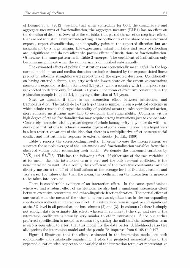
The duration of declines 61
of Desmet et al. (2012), we find that when controlling for both the disaggregate andaggregate measures of fractionalization, the aggregate measure (ELF1) has no effect onthe duration of declines. Several of the variables that passed the selection step have effectsthat are not robust in a multivariate setting. The coefficients of the share of manufacturedexports, export diversification, and inequality point in the expected direction but areinsignificant by a large margin. Life expectancy, infant mortality and years of schoolingare insignificant and do not affect the partial effects of institutions or fractionalization.Otherwise, the same pattern as in Table 2 emerges. The coefficient of institutions onlybecomes insignificant when the sample size is diminished substantially.
The estimated effects of political institutions are economically meaningful. In the log-normal model, mean and median duration are both estimated by the exponentiated linearprediction allowing straightforward predictions of the expected duration. Conditionallyon having entered a slump, a country with the lowest score on the executive constraintsmeasure is expected to decline for about 9.1 years, while a country with the highest scoreis expected to decline only for about 3.1 years. The mean of executive constraints in theestimation sample is about 2.4, implying a duration of 7.1 years.
Next we examine if there is an interaction effect between institutions andfractionalization. The rationale for this hypothesis is simple. Given a political economy inwhich ethnic tension challenges the ability of political actors to take coordinated action,more cohesive institutions may help to overcome this vulnerability. Countries with ahigh degree of ethnic fractionalization may require strong institutions just to compensate.Conversely, countries with a greater degree of ethnic homogeneity may make do with lessdeveloped institutions to achieve a similar degree of social coordination. This hypothesisis a less restrictive variant of the idea that there is a multiplicative effect between socialconflict and institutions in response to external shocks (Rodrik, 1999).
Table 3 reports the corresponding results. In order to ease the interpretation, wesubtract the sample average of the institutions and fractionalization variables from theirobserved values before estimating each model. We denote the demeaned variables by
INS0 and ELF15. This has the following effect. If either one of the two variables isat its mean, then the interaction term is zero and the only relevant coefficient is thenon-interacted variant. As a result, the coefficient of the executive constraints variabledirectly measures the effect of institutions at the average level of fractionalization, andvice versa. For values other than the mean, the coefficient on the interaction term needsto be taken into account.
There is considerable evidence of an interaction effect. In the same specificationswhere we find a robust effect of institutions, we also find a significant interaction effectbetween executive constraints and ethno-linguistic fractionalization. The partial effect ofone variable at the mean of the other is at least as significant as in the correspondingspecification without an interaction effect. The interaction term is negative and significantat the 5%-level in all perturbations but columns (2) and (3). In column (2) there is simplynot enough data to estimate this effect, whereas in column (3) the sign and size of theinteraction coefficient is actually very similar to other estimations. Since our earlierpreferred specification is nested in column (6), testing the null that the interaction termis zero is equivalent to a test that this model fits the data better. A likelihood ratio testalso prefers the interaction model and the pseudo-R2 improves from 0.168 to 0.197.
Figure 4 illustrates that the effects estimated in the interaction model are botheconomically and statistically significant. It plots the predicted semi-elasticities of theexpected duration with respect to one variable of the interaction term over representative

62 Chapter 3. Do weak institutions prolong crises?
Table 3 – Interaction effects of institutions and fractionalization
(1) (2) (3) (4) (5) (6)Variables ln t ln t ln t ln t ln t ln t
Executive Constraints (INS0) -0.366*** -0.137 -0.091 -0.280*** -0.217** -0.288***(0.098) (0.126) (0.101) (0.090) (0.087) (0.080)
Fractionalization (ELF15) 0.016*** 0.016*** 0.019*** 0.017*** 0.017*** 0.018***(0.004) (0.006) (0.004) (0.004) (0.004) (0.004)
INS0 × ELF15 -0.005*** 0.000 -0.003 -0.004** -0.003** -0.004***(0.002) (0.002) (0.002) (0.002) (0.001) (0.001)
Initial ln GDP per capita 0.275** 1.007*** 0.238* 0.533*** 0.439*** 0.198*(0.123) (0.293) (0.135) (0.175) (0.163) (0.106)
Real US Interest Rate 0.068 0.064 0.100* 0.084* 0.076* 0.098**(0.042) (0.072) (0.054) (0.043) (0.042) (0.047)
Trade Openness (de jure) -0.690**(0.298)
Trade Openness (de facto) 0.015***(0.005)
Manufactures (% Exports) -0.008(0.012)
Export Diversification -0.004(0.011)
Export Sophistication -1.503*(0.784)
Private Credit -0.008(0.009)
Financial Depth -0.008(0.011)
Infant Mortality 0.001(0.007)
Life Expectancy -0.020(0.030)
Education (All) -0.045(0.070)
Constant -1.122 6.940 0.213 -1.425 -2.552* 0.025(0.910) (4.896) (1.247) (2.066) (1.362) (0.872)
Region FE NO NO NO NO YES NOExits 42 18 25 45 47 47Spells 51 22 32 55 57 57Years of Decline 314 166 193 325 346 346Log-L -54.001 -22.648 -35.514 -62.746 -61.681 -69.540Pseudo-R2 0.315 0.278 0.238 0.243 0.288 0.197
Note(s): The standard errors are cluster-robust at the country level. *** p<0.01, ** p<0.05, *p<0.1
values of the other, including a 95% confidence interval. Three points stand out: 1) theeffect of executive constraints clearly depends on fractionalization (and vice versa), 2)both partial effects are significant over most of the distribution, and 3) both partialeffects consistently have the expected sign. In the background, Figure 4 also showshistograms of the sample data. Executive constraints scores cover the entire range from1 to 7, and ethno-linguistic fractionalization ranges from near-zero (0.07%) to near-totalheterogeneity (96%). The predictions cover a wide range of the durations. At theaverage score of executive constraints, a country with the highest (lowest) degree of ethnicheterogeneity is expected to decline for about 12.6 years (2.1 years). Hence, it would bedifficult to understand the effects of institutions without considering fractionalization.Stronger institutions also have the potential to overcome the adverse effects of high levelsof ethnic fractionalization. At the 75th percentile of ethnic heterogeneity (ELF15 = 89.7),a country with the highest (lowest) score of executive constraints is expected to declinefor about 1.8 years (18.3 years).

The duration of declines 63
Figure 4 – Partial Effects in Interaction Model
(a) Fractionalization (ELF15)
0.1
.2.3
.4P
art
ial E
ffe
ct
of
Fra
ctio
na
liza
ton (
ELF
15)
0.2
5.5
.75
1F
ractio
n o
f D
ata
1 2 3 4 5 6 7Executive Constraints (INS0)
(b) Executive Constraints (INS0)
−1
0−
8−
6−
4−
20
Pa
rtia
l E
ffe
ct
of
Exe
cu
tive
Co
nstr
ain
ts (
INS
0)
0.2
5.5
.75
1F
ractio
n o
f D
ata
0 25 50 75 100Fractionalization (ELF15)
Note(s): The partial effects are based on column (6) in Table 3 and are computed over the entirerange of the variable on the horizontal axis while keeping all other regressors at their means. Thedashed lines are upper and lower 95% confidence limits.
One way to interpret the effects of fractionalization and institutions is through the lensof the delayed stabilizations literature (Alesina and Drazen, 1991). When (ethnic) groupsengage in a ‘war of attrition’ over the burden of reform and are uncertain about how thereform benefits all other groups (hence their willingness to bear the costs), then policyreform is delayed until the weakest group concedes. The expected time until stabilizationoccurs is expected to increase with the number of groups involved in the decision-makingprocess and the veto points they possess, so that the adjustment speed depends on thepolitical system (Spolaore, 2004). However, this interpretation does not explain the stronginteraction effect between executive constraints and ethnic heterogeneity very well.
We propose a theoretical mechanism whereby groups facing a crisis have to decide ona policy response under uncertainty about post-crisis outcomes. When the executive isunconstrained, then some groups may have an incentive to delay cooperation by fear ofboosting the strength of the independent executive and its power to expropriate them inthe aftermath of the crisis. If groups can fortify their position through blocking agreementon policy, then such a mechanism could generate the observed interaction.11
Robustness
We briefly illustrate that our main conclusions are unaffected by the choice of the baselinehazard, extending the sample and adding unobserved heterogeneity, the exclusion ofinfluential regions, and different ways of accounting for recurrent spells. In addition, wealso analyze the depth of the decline and the average rate of contraction.
Table 4 tackles the issues of functional form and model selection. We reportour preferred specification in the first column and then show estimates based on fivealternative forms of the hazard function. Column (2) uses a log-logistic hazard insteadof the log-normal shape. The estimated shape parameter (ln γ) is negative, implyingthat the hazard is first increasing then decreasing as in the log-normal model. This
11In Chapter 4 we formalize this mechanism and provide a theory of delayed responses to crises.

64 Chapter 3. Do weak institutions prolong crises?
Table 4 – Robustness: functional form
(1) (2) (3) (4) (5) (6)Log-normal Log-logistic Exponential Weibull Gompertz Cox PH
Variables ln t ln t ln t ln t ln t ln tCoefficients Hazard Ratios (H0 : HR = 1)
Executive Constraints (INS0) -0.178*** -0.185*** 1.229*** 1.263*** 1.222*** 1.221***(0.058) (0.067) (0.074) (0.089) (0.071) (0.082)
Fractionalization (ELF15) 0.016*** 0.016*** 0.978*** 0.974*** 0.979*** 0.979***(0.004) (0.005) (0.005) (0.007) (0.005) (0.006)
Initial ln GDP per capita 0.197* 0.235** 0.787 0.765 0.786* 0.768(0.106) (0.112) (0.119) (0.146) (0.113) (0.137)
Real US Interest Rate 0.087* 0.084* 0.947 0.928 0.949 0.951(0.048) (0.051) (0.058) (0.061) (0.057) (0.064)
lnσ (Log-normal) -0.065(0.093)
ln γ (Log-logistic) -0.580***(0.105)
ln p (Weibull) 1.219**(0.107)
γ (Gompertz) 0.985(0.030)
Constant -0.553 -0.856 1.830 1.723 1.928(0.868) (0.901) (2.432) (2.884) (2.448)
Exits 47 47 47 47 47 47Spells 57 57 57 57 57 57Years of Decline 346 346 346 346 346 346Log-L -72.090 -73.286 -75.295 -73.940 -75.192 -143.142AIC 156.180 158.571 160.590 159.879 162.384 294.285Pseudo-R2 0.168 0.164 0.208 0.210 0.160 0.088
Note(s): The standard errors are cluster-robust at the country level. *** p<0.01, ** p<0.05, *p<0.1.
lends itself to the following interpretation. In the first few years of a decline, somecountries are able to recover quickly. However, the longer the decline lasts, the moreeconomic fundamentals deteriorate making it increasingly difficult to enter a recovery.Columns (3) to (6) have a different interpretation. We no longer report coefficientsbut instead hazard ratios, since these models are proportional hazards (PH) models bynature. They are interpreted as follows. A hazard ratio greater than one implies a higherinstantaneous probability of exiting the decline. A hazard ratio smaller than one impliesa lower instantaneous probability of exiting the decline. Column (3) is the exponential orconstant hazard model. The results remain very similar (given the altered interpretation),but the log-likelihood decreases somewhat. Column (4) uses a Weibull parameterizationwhich allows for monotonically increasing or decreasing hazard rates. This model alsohas a shape parameter (p) which allows testing for whether the rate increases, decreasesor is constant. The estimate suggests that the baseline hazard is increasing over time. Incontrast, the Gompertz model in column (5) also suggests a shape that is monotonicallydecreasing (γ < 0). Among these parametric models, the AIC is lowest for the log-normaldistribution; that is, our preferred model fits the data best. In column (6), we specify asemi-parametric Cox model which does not restrict the shape of the baseline hazard. TheCox model also suggests that the probability of exiting a spell first increases very brieflyand then decreases monotonically. However, the imposed proportional hazard restrictioncomes at a great cost in terms of fit.
The previous section has already shown that the findings are robust to the inclusionof regional fixed effects. Column (1) in Table 5 goes two steps further: it extends the
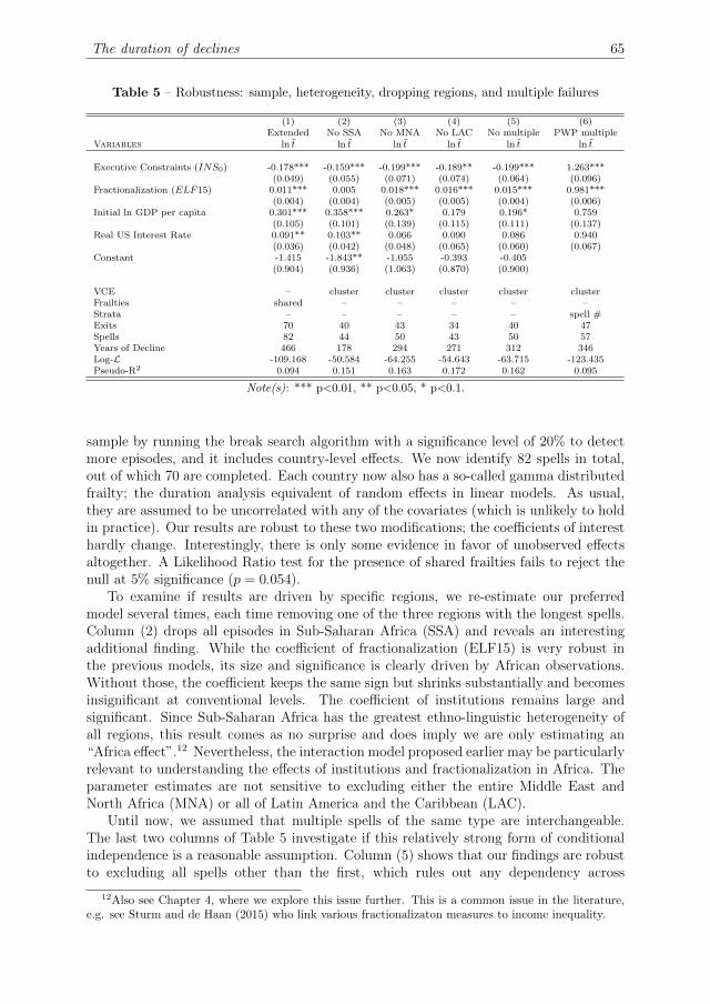
The duration of declines 65
Table 5 – Robustness: sample, heterogeneity, dropping regions, and multiple failures
(1) (2) (3) (4) (5) (6)Extended No SSA No MNA No LAC No multiple PWP multiple
Variables ln t ln t ln t ln t ln t ln t
Executive Constraints (INS0) -0.178*** -0.159*** -0.199*** -0.189** -0.199*** 1.263***(0.049) (0.055) (0.071) (0.074) (0.064) (0.096)
Fractionalization (ELF15) 0.011*** 0.005 0.018*** 0.016*** 0.015*** 0.981***(0.004) (0.004) (0.005) (0.005) (0.004) (0.006)
Initial ln GDP per capita 0.301*** 0.358*** 0.263* 0.179 0.196* 0.759(0.105) (0.101) (0.139) (0.115) (0.111) (0.137)
Real US Interest Rate 0.091** 0.103** 0.066 0.090 0.086 0.940(0.036) (0.042) (0.048) (0.065) (0.060) (0.067)
Constant -1.415 -1.843** -1.055 -0.393 -0.405(0.904) (0.936) (1.063) (0.870) (0.900)
VCE – cluster cluster cluster cluster clusterFrailties shared – – – – –Strata – – – – – spell #Exits 70 40 43 34 40 47Spells 82 44 50 43 50 57Years of Decline 466 178 294 271 312 346Log-L -109.168 -50.584 -64.255 -54.643 -63.715 -123.435Pseudo-R2 0.094 0.151 0.163 0.172 0.162 0.095
Note(s): *** p<0.01, ** p<0.05, * p<0.1.
sample by running the break search algorithm with a significance level of 20% to detectmore episodes, and it includes country-level effects. We now identify 82 spells in total,out of which 70 are completed. Each country now also has a so-called gamma distributedfrailty; the duration analysis equivalent of random effects in linear models. As usual,they are assumed to be uncorrelated with any of the covariates (which is unlikely to holdin practice). Our results are robust to these two modifications; the coefficients of interesthardly change. Interestingly, there is only some evidence in favor of unobserved effectsaltogether. A Likelihood Ratio test for the presence of shared frailties fails to reject thenull at 5% significance (p = 0.054).
To examine if results are driven by specific regions, we re-estimate our preferredmodel several times, each time removing one of the three regions with the longest spells.Column (2) drops all episodes in Sub-Saharan Africa (SSA) and reveals an interestingadditional finding. While the coefficient of fractionalization (ELF15) is very robust inthe previous models, its size and significance is clearly driven by African observations.Without those, the coefficient keeps the same sign but shrinks substantially and becomesinsignificant at conventional levels. The coefficient of institutions remains large andsignificant. Since Sub-Saharan Africa has the greatest ethno-linguistic heterogeneity ofall regions, this result comes as no surprise and does imply we are only estimating an“Africa effect”.12 Nevertheless, the interaction model proposed earlier may be particularlyrelevant to understanding the effects of institutions and fractionalization in Africa. Theparameter estimates are not sensitive to excluding either the entire Middle East andNorth Africa (MNA) or all of Latin America and the Caribbean (LAC).
Until now, we assumed that multiple spells of the same type are interchangeable.The last two columns of Table 5 investigate if this relatively strong form of conditionalindependence is a reasonable assumption. Column (5) shows that our findings are robustto excluding all spells other than the first, which rules out any dependency across
12Also see Chapter 4, where we explore this issue further. This is a common issue in the literature,e.g. see Sturm and de Haan (2015) who link various fractionalizaton measures to income inequality.

66 Chapter 3. Do weak institutions prolong crises?
recurrent spells. The coefficient of executive constraints becomes even larger and theeffect of fractionalization is virtually unchanged. Column (6) takes a different approachand specifies a conditional risk set model or stratified Cox model due to Prentice et al.(1981, PWP). The model accounts for ordering of the events but assumes that a subjectcannot experience another event until the previous event has occurred. This is a naturalassumption, as – by definition – a country cannot exit a second decline phase beforehaving left the first. The results (hazard ratios) are qualitatively similar.
Table 6 – Robustness: Average rate of decline and total depth
(1) (2) (3) (4) (5) (6)Variables gi gi tD × gi tD × gi tD × gi tD × gi
Executive Constraints (INS0) 0.003 0.001 0.034*** 0.005 0.027** 0.002(0.002) (0.002) (0.010) (0.010) (0.010) (0.012)
Fractionalization (ELF15) -0.000 -0.000* -0.003*** -0.005*** -0.003*** -0.005***(0.000) (0.000) (0.001) (0.001) (0.001) (0.001)
Interaction (INS0 × ELF15) 0.000* 0.001*** 0.001***(0.000) (0.000) (0.000)
Initial ln GDP per capita -0.001 -0.001 -0.022 -0.022 -0.052 -0.045(0.006) (0.006) (0.024) (0.024) (0.033) (0.035)
Real US Interest Rate -0.002 -0.002 -0.001 -0.006 0.001 -0.003(0.002) (0.002) (0.009) (0.008) (0.009) (0.008)
Constant -0.030 -0.022 0.007 0.098 0.308 0.352(0.049) (0.049) (0.197) (0.186) (0.310) (0.310)
Region FE NO NO NO NO YES YESSpells 57 57 57 57 57 57Log-L 106.795 107.408 12.267 14.939 15.987 18.209R2 0.009 0.011 0.289 0.340 0.295 0.333
Note(s): Standard errors are cluster-robust at the country level. *** p<0.01, ** p<0.05, * p<0.1.
Last but not least, we construct a simple test to examine whether the effects ofinstitutions and ethnic cleavages on the depth of a slump run solely through the durationprocess or if they also affect the rate of contraction. Since the depth of the decline isthe product of the estimated duration and the average rate of contraction, we can definegi ≡
(yi,tmin − yi0
)/(tmin − t0) ≡
(yi,tmin − yi0
)/tD as the average rate of decline and
tD × gi ≡ yi,tmin − yi0 as the overall depth of the decline. Here yit is still the log of GDPper capita in country i at time t, and gi is by construction negative. We have alreadyanalyzed the duration of declines. Now we run OLS regressions explaining the rate ofcontraction (gi) and depth (tD × gi) to isolate the channel through which the previouslyestimated effects run.
Column (1) in Table 6 shows that we find no evidence in favor of an effect of eitherexecutive constraints or fractionalization on the average rate of decline. Column (2)confirms the absence of robust effects for the specification with an interaction term.In fact, in both columns most coefficients are insignificant and estimated to be virtuallyzero. The variables are not mean-centered in this case. The remaining columns of Table 6examine the depth of the slump. Columns (3) and (4) illustrate that we now recover thepreviously estimated effects (even with similar significance levels and, naturally, withreversed signs since gi is negative). These results are robust to the inclusion of regionfixed effects as shown in columns (5) and (6). The interaction models explain about33–34% of the variation in depth, highlighting the relevance of the estimated effects.Together with the duration analysis and the analysis of the average rate of decline, thisleads us to conclude that a) political institutions and ethnic heterogeneity have robust

Concluding remarks 67
effects on the overall depth of slumps, and b) these effects run primarily through theduration of the decline phase and not the rate of contraction.
5 Concluding remarks
This chapter makes several contributions to a burgeoning literature on growth episodesand structural breaks in growth performances. We show that a restricted structuralchange approach, as in Papell and Prodan (2012), works well as an inferential methodfor identifying slumps, big recessions or growth collapses in a large sample of countries.We find a substantial number of slumps in developing and developed countries alike,suggesting that severe downward volatility is an ubiquitous phenomenon in the post-war period. There is systematic evidence of weak political institutions before slumpshit and positive institutional change during and in the immediate aftermath of slumps.Our interpretation of this stylized fact is that, while institutions may cause growth,volatility can also contribute to endogenous institutional change. Severe economic crisesbring about what we may call creative political destruction and raise the pressurefor institutional reform in a very broad sense. Our key finding is that the durationof declines depends on institutions and also particularly strongly on ethno-linguisticfractionalization. An important extension is that the effect of executive constraints isnon-linear and depends on the level of fractionalization, an interaction which is notfully captured by current theories of policy reform and delay. We also show that effectsof political institutions and ethnic cleavages on the depth of declines run through theduration.
As a whole, our results lend broad support to political economy theories emphasizingthe respective roles of institutions and ethnic cleavages. Effective coordination andresponses to slumps are hampered by a high degree of social tension as captured byethno-linguistic fractionalization. However, particularly strong political institutions canput in place coordination mechanisms that are able to contain or resolve these conflictswithin the institutional framework. At the same time, our findings imply that in lessethnically fragmented societies political institutions are less important as a determinantof the length of declines.
These results do not suggest that sound macroeconomic policies as such do not matter,though they provide some indication that these policies may be secondary to morefundamental factors. We need more research on which specific institutional features allowbetter policies to emerge. While the previous literature has stressed the role of positivegrowth spurts, we show that slumps matter a lot and that the decline phase can lastvery long in some cases. We think a comparison of the relative effects of slumps versusaccelerations on long-run GDP levels would be an interesting extension of our findings.

68 Bibliography
Bibliography
Acemoglu, D. and S. Johnson (2005). Unbundling institutions. Journal of Political Economy 113 (5),949–95.
Acemoglu, D., S. Johnson, and J. A. Robinson (2001). The colonial origins of comparative development:An empirical investigation. American Economic Review 91 (5), 1369–1401.
Acemoglu, D., S. Johnson, and J. A. Robinson (2002). Reversal of Fortune: Geography and Institutionsin the Making of the Modern World Income Distribution. Quarterly Journal of Economics 117 (4),1231–1294.
Acemoglu, D., S. Johnson, J. A. Robinson, and Y. Thaicharoen (2003). Institutional causes,macroeconomic symptoms: volatility, crises and growth. Journal of Monetary Economics 50 (1),49–123.
Acemoglu, D. and J. A. Robinson (2006). Economic Origins of Democracy and Dictatorship. CambridgeUniversity Press.
Aguiar, M. and G. Gopinath (2007). Emerging market business cycles: The cycle is the trend. Journalof Political Economy 115 (1), 69–102.
Alesina, A. and A. Drazen (1991). Why are stabilizations delayed? American Economic Review 81 (5),1170–1188.
Alesina, A. and E. L. Ferrara (2005). Ethnic diversity and economic performance. Journal of EconomicLiterature 43 (3), 762–800.
Ashraf, Q. and O. Galor (2013). The “Out of Africa” hypothesis, human genetic diversity, andcomparative economic development. American Economic Review 103 (1), 1–46.
Bai, J. (1997). Estimating multiple breaks one at a time. Econometric Theory 13, 315–352.
Bai, J. (1999). Likelihood ratio tests for multiple structural changes. Journal of Econometrics 91 (2),299–323.
Bai, J. and P. Perron (1998). Estimating and testing linear models with multiple structural changes.Econometrica 66, 47–78.
Bai, J. and P. Perron (2003). Computation and analysis of multiple structural change models. Journalof Applied Econometrics 18 (1), 1–22.
Barro, R. J. and J.-W. Lee (2010, April). A new data set of educational attainment in the world,1950-2010. Working Paper 15902, National Bureau of Economic Research.
Beck, T., A. Demirguc-Kunt, and R. Levine (2010). Financial institutions and markets across countriesand over time: The updated financial development and structure database. World Bank EconomicReview 24 (1), 77–92.
Ben-David, D. and D. H. Papell (1995). The great wars, the great crash, and steady state growth: Somenew evidence about an old stylized fact. Journal of Monetary Economics 36 (3), 453–475.
Berg, A., J. D. Ostry, and J. Zettelmeyer (2012). What makes growth sustained? Journal of DevelopmentEconomics 98 (2), 149–166.
Besley, T. and T. Persson (2011). The logic of political violence. Quarterly Journal of Economics 126 (3),1411–1445.
Cameron, A. C., J. B. Gelbach, and D. L. Miller (2011). Robust inference with multiway clustering.Journal of Business & Economic Statistics 29 (2), 238–249.
Cerra, V. and S. C. Saxena (2008). Growth dynamics: The myth of economic recovery. AmericanEconomic Review 98 (1), 439–57.
Chinn, M. D. and H. Ito (2006). What matters for financial development? capital controls, institutions,and interactions. Journal of Development Economics 81 (1), 163–192.
Desmet, K., I. Ortuno-Ortın, and R. Wacziarg (2012). The political economy of linguistic cleavages.Journal of Development Economics 97 (2), 322–338.
Diebold, F. X. and C. Chen (1996). Testing structural stability with endogenous breakpoint a sizecomparison of analytic and bootstrap procedures. Journal of Econometrics 70 (1), 221–241.
Easterly, W., M. Kremer, L. Pritchett, and L. Summers (1993). Good policy or good luck? Journal ofMonetary Economics 32 (3), 459–483.
Eichengreen, B., A. K. Rose, and C. Wyplosz (1995). Exchange market mayhem: the antecedents andaftermath of speculative attacks. Economic Policy 10 (21), 249–312.
Fernandez, R. and D. Rodrik (1991). Resistance to reform: Status quo bias in the presence of individual-specific uncertainty. American Economic Review 81 (5), 1146–1155.

Bibliography 69
Gleditsch, N. P., P. Wallensteen, M. Eriksson, M. Sollenberg, and H. Strand (2002). Armed conflict1946-2001: A new dataset. Journal of Peace Research 39 (5), 615–637.
Goemans, H. E., K. S. Gleditsch, and G. Chiozza (2009). Introducing Archigos: A dataset of politicalleaders. Journal of Peace Research 46 (2), 269–283.
Gourinchas, P.-O. and M. Obstfeld (2012). Stories of the twentieth century for the twenty-first. AmericanEconomic Journal: Macroeconomics 4 (1), 226–265.
Hansen, B. E. (2000). Testing for structural change in conditional models. Journal of Econometrics 97 (1),93–115.
Hausmann, R., J. Hwang, and D. Rodrik (2007). What you export matters. Journal of EconomicGrowth 12 (1), 1–25.
Hausmann, R., L. Pritchett, and D. Rodrik (2005). Growth accelerations. Journal of EconomicGrowth 10 (4), 303–329.
Hausmann, R., F. Rodriguez, and R. Wagner (2008). Growth collapses. In C. Reinhart, C. Vegh, andA. Velasco (Eds.), Money, Crises and Transition, pp. 376–428. Cambridge, Mass.: MIT Press.
Jerzmanowski, M. (2006). Empirics of hills, plateaus, mountains and plains: A markov-switchingapproach to growth. Journal of Development Economics 81 (2), 357–385.
Jones, B. F. and B. A. Olken (2008). The anatomy of start-stop growth. Review of Economics andStatistics 90 (3), 582–587.
Kalbfleisch, J. D. and R. L. Prentice (2002). The statistical analysis of failure time data (2nd ed.). NewYork: John Wiley.
Lancaster, T. (1990). The econometric analysis of transition data. Cambridge University Press.
Lane, P. R. and G. M. Milesi-Ferretti (2007). The external wealth of nations mark ii: Revisedand extended estimates of foreign assets and liabilities, 1970-2004. Journal of InternationalEconomics 73 (2), 223–250.
MacKinnon, J. (2009). Bootstrap hypothesis testing. In D. Belsley and E. Kontoghiorghes (Eds.),Handbook of Computational Econometrics, Chapter 6, pp. 183–213. John Wiley & Sons, Ltd.
Mobarak, A. (2005). Democracy, volatility, and economic development. Review of Economics andStatistics 87 (2), 348–361.
Nelson, C. R. and C. R. Plosser (1982). Trends and random walks in macroeconmic time series: someevidence and implications. Journal of Monetary Economics 10 (2), 139–162.
North, D. C., J. Wallis, and B. Weingast (2009). Violence and Social Orders A Conceptual Frameworkfor Interpreting Recorded Human History. Cambridge University Press.
Papell, D. H. and R. Prodan (2012). The Statistical Behavior of GDP after Financial Crises and SevereRecessions. The B.E. Journal of Macroeconomics 12 (3), 1–31.
Prentice, R. L., B. J. Williams, and A. V. Peterson (1981). On the regression analysis of multivariatefailure time data. Biometrika 68 (2), 373–379.
Pritchett, L. (2000). Understanding patterns of economic growth: searching for hills among plateaus,mountains, and plains. World Bank Economic Review 14 (2), 221–250.
Prodan, R. (2008). Potential pitfalls in determining multiple structural changes with an application topurchasing power parity. Journal of Business & Economic Statistics 26 (1), 50–65.
Ramey, G. and V. A. Ramey (1995). Cross-country evidence on the link between volatility and growth.American Economic Review 85 (5), 1138–1151.
Rodrik, D. (1999). Where did all the growth go? External shocks, social conflict, and growth collapses.Journal of Economic Growth 4 (4), 385–412.
Solt, F. (2009). Standardizing the World Income Inequality Database. Social Science Quarterly 90 (2),231–242. SWIID Version 3.0, July 2010.
Spolaore, E. (2004). Adjustments in different government systems. Economics & Politics 16 (2), 117–146.
Sturm, J.-E. and J. de Haan (2015). Income inequality, capitalism and ethno-linguistic fractionalization.American Economic Review: Papers and Proceedings. forthcoming.
Wacziarg, R. and K. H. Welch (2008). Trade liberalization and growth: New evidence. World BankEconomic Review 22 (2), 187–231.
Wooldridge, J. M. (2010). Econometric analysis of cross section and panel data (2nd ed.). The MITpress.
Zivot, E. and D. W. K. Andrews (1992). Further evidence on the great crash, the oil-price shock, andthe unit-root hypothesis. Journal of Business & Economic Statistics 10 (3), 251–270.

70 Appendix
Appendix A: Estimation of structural breaks
Sequential procedure for testing and dating breaks
The procedure described here is a modification of Bai’s (1997) sequential likelihood ratiotests for structural change – see also the extensions in Bai and Perron (1998) and in Bai(1999). We make an important simplifying assumption, namely, that all output seriesare regime-wise trend-stationary. Verifying this assumption is beyond the scope of thischapter, as testing for unit roots in the presence of structural breaks (with sufficientpower and size) is still contested territory and our output series have only a moderatetime dimension (T < 60 years). We implement the sequential procedure in six steps.
1. Determine the optimal AR(p) trend model using the Bayesian information criterionto adjust for serial correlation up to a maximum lag count (pmax). We set pmax = 4.
2. Specify the partial structural change model:
yt = α+βt+γ01(t > tb1)+γ1(t−tb1)1(t > tb1)+γ2(t−tb2)1(t > tb2)+
p∑
i=1
δiyt−i+εt
where yt is the log of GDP per capita in year t, tbi are the possible break dates,1(·) is an indicator function, and p is the lag order as determined by the optimalAR(p) model. We require that tb2 ≥ tb1 + h for h = 4. In other words, the periodbetween two successive breaks making up the same episode is at minimum 4 years.
3. Define trimming parameter τ , where typically τ ∈ [0.05, 0.25]. The breaks are inthe ranges tb1 ∈ [τT, (1− τ)T − h] and tb2 ∈ [τT + h, (1− τ)T ]. We set τ = 0.05.Let Λτ denote the set of all possible episodes [tb1, tb2] ⊂ [τT, (1− τ)T ].13
4. Compute the sup-W test statistic of the null of no break versus at least one break(H0 : γ0 = γ1 = γ2 = 0). The supremum is taken over all episodes in Λτ with apositive estimate of β and a non-positive estimate of γ0:
sup[tb1,tb2]∈Λτ
W (tb1, tb2) = sup[tb1,tb2]∈Λτ
(T −K
3
)SSRr − SSRu
SSRu
where K is the number of parameters, SSRr denotes the sum of squared residualsfrom a regression imposing H0, and SSRu the sum of squared residuals from aregression imposing only β > 0 and γ0 ≤ 0.
5. The critical value and empirical p-value of sup-W statistic is bootstrapped.14
6. If the sup-W statistic is significant at the desired level, the remaining sample is splitinto two new sub-samples from the beginning to the first break and from the secondbreak to the end, then the procedure restarts at (4) using the estimated AR-orderfrom before. If the bootstrapped sup-W ∗ test fails to reject in each sub-sample, orthe sub-samples are too small (T ≤ 20), then the procedure stops.
13For simplicity of exposition, we suppress an additional index running over the sub-samples (definedin Step 6). T refers to the number of observations of the currently active sample. The notation neglectsthe discontinuity of actual observation times.
14In finite samples comparable asymptotic tests often have poor size and power (see Prodan, 2008).

Appendix 71
Bootstrapping the sup-Wald statistic
There have been several suggestions on how to best bootstrap structural change testsin particular or other popular time series tests in general. For example, Hansen(2000) suggests employing a fixed-design bootstrap allowing for non-stationarity, laggeddependent variables and conditional heteroskedasticity. MacKinnon (2009), on thecontrary, shows that the recursive bootstrap of Diebold and Chen (1996) gives resultssuperior to most other bootstrap types (fixed-parameter, sieve, pairs, block, doubleblock) as well as the asymptotic test in a simple application of an AR(1) model with anendogenous break. Papell and Prodan (2012) also favor a recursive bootstrap though theydo not compare it to other methods. We use a recursive bootstrap similar to Diebold andChen (1996). Comparing methods systematically is beyond the scope of this chapter.15
In line with usual notation, we denote all bootstrap quantities with the superscript ‘∗’.The bootstrap procedure is as follows.
1. Specify the optimal break model under the H0 of no structural breaks in the specifiedsample using the BIC as before and obtain the residuals:
et = yt − α− βt−p∑
i=1
δiyt−i.
2. Draw new residuals: e∗t = ut, with ut ∼ i.i.d. N (0, σ2e).
3. Construct a bootstrap sample of equal size as the original sample:
y∗t = α + βt+
p∑
i=1
δiy∗t−i + e∗t , ∀t = 1 + p, . . . , T
where y∗t−i is the observed yt−i only in the case of a fixed-design bootstrap, otherwisey∗t must be constructed recursively (conditional on p observed initial values).
4. Rerun the break search algorithm on the bootstrap series y∗t , includingdetermination of the optimal AR(p) model, and compute bootstrapped teststatistics sup[tb∗1,tb
∗2]∈Λτ W
∗j , where j indexes the current bootstrap iteration.
5. Repeat from Step (2) until j = B, where B is the total number of bootstrapreplications. We set B = 1000.
6. The bootstrap p-value (p∗) is obtained by counting the proportion of the estimatedbootstrap test statistics that are greater than the originally calculated test statistic:
p∗ =1
B
B∑
j=1
1
(sup
[tb∗1,tb∗2]∈Λτ
W ∗j > sup
[tb1,tb2]∈Λτ
W (tb1, tb2)
).
The critical value is the (1−αs)Bth largest bootstrapped sup-W ∗ statistic, where αs
is the desired significance level (10% throughout the text, unless otherwise noted).
15We use a parametric recursive bootstrap, but informally compared the results to other techniques.Hansen’s fixed-design bootstrap generates (too) many questionable slumps and the Wild bootstrap rejects(too) often. Residual and parametric bootstraps give similar results.

72 Appendix
Appendix B: List of episodes
Table B-1 – Global Parameters
Data: PWT Max AR (pmax): 4Sample start: 1950 Bootstrap replications: 1000Sample end: 2008 Bootstrap errors: parametricTrimming (τ): 0.05 Bootstrap type: recursiveMin. tbi distance (h): 4 Bootstrap significance (αs): 0.1
Table B-2 – Estimated and Filtered Breaks with Troughs: 58 Episodes*
Code T0 tb1 tmin tb2 T Sup-W Critical W p-value Drop (%) Duration cALB 1970 1990 1991 2002 2008 18.5 13.6 0.007 -15.32 1 0ARE 1986 1990 1999 2002 2008 29.1 14.5 0.003 -10.90 9 0AUS 1950 1954 1957 1966 2008 8.3 8.7 0.064 -0.72 3 0AUS 1967 1989 1991 1998 2008 10.1 10.7 0.059 -2.29 2 0BDI 1960 1971 1972 1988 2008 9.9 11.3 0.089 -3.23 1 0BEL 1950 1957 1958 1973 2008 12.8 12.1 0.029 -2.24 1 0BGR 1970 1988 1997 1997 2008 16.3 12.8 0.010 -23.79 9 0BHR 1970 1980 1987 1986 2008 14.4 11.0 0.010 -44.12 7 1BRA 1950 1980 1983 2003 2008 12.5 12.3 0.043 -14.60 3 0CAF 1960 1978 2005 2005 2008 8.3 8.7 0.060 -46.38 27 1CHE 1950 1974 1975 1978 2008 10.7 10.6 0.047 -7.87 1 0CHL 1951 1953 1954 1972 1973 12.0 8.5 0.017 -9.06 1 0CHL 1951 1974 1975 1979 1980 13.3 10.8 0.021 -16.50 1 0CHL 1951 1981 1983 1995 2008 12.6 11.4 0.025 -21.22 2 0CHN 1952 1960 1962 1977 2008 13.9 12.9 0.029 -23.71 2 0CMR 1960 1986 1995 1990 2008 12.0 12.3 0.055 -40.46 9 1COG 1960 1974 1977 1982 2008 11.9 12.5 0.069 -21.35 3 0CRI 1950 1955 1956 1963 1979 11.4 11.3 0.048 -4.39 1 0CRI 1950 1980 1982 2002 2008 17.2 10.6 0.002 -17.47 2 0CUB 1970 1988 1993 1995 2008 11.4 12.5 0.072 -34.70 5 0CYP 1950 1973 1975 1977 2008 15.5 9.7 0.001 -31.40 2 0CYP 1978 1990 1991 1995 2008 11.6 14.6 0.098 -10.19 1 0DNK 1950 1954 1955 1965 2008 12.9 11.7 0.022 -1.56 1 0DZA 1960 1984 1994 1996 2008 10.9 8.2 0.013 -14.09 10 0ETH 1950 1972 1992 1993 2008 11.5 10.2 0.020 -30.68 20 0FIN 1950 1989 1993 2006 2008 10.6 10.8 0.057 -16.34 4 0GAB 1960 1976 1987 1997 2008 10.6 11.2 0.062 -50.56 11 1GMB 1960 1982 1998 2002 2008 16.4 11.2 0.006 -25.33 16 0GRC 1951 1973 1974 1994 2008 17.9 11.6 0.003 -6.92 1 0GTM 1950 1980 1988 1984 2008 15.1 12.3 0.015 -19.14 8 0HUN 1970 1990 1992 2004 2008 15.6 13.5 0.018 -10.56 2 0IDN 1960 1997 1999 2001 2008 13.5 10.6 0.013 -17.49 2 0IRN 1955 1976 1981 1980 2008 15.9 11.6 0.004 -56.78 5 1IRQ 1970 1990 2003 1994 2008 9.1 8.9 0.046 -66.43 13 1JPN 1950 1973 1974 1990 2008 13.5 13.4 0.050 -2.85 1 0MEX 1950 1981 1988 1995 2008 11.9 11.0 0.038 -17.03 7 0MNG 1970 1990 1993 2003 2008 46.5 11.7 0.000 -41.81 3 0MOZ 1960 1981 1986 1995 2008 12.6 12.0 0.037 -24.99 5 0MYS 1955 1984 1986 1993 2008 9.1 10.5 0.093 -7.47 2 0NPL 1960 1979 1980 2000 2008 10.6 8.9 0.025 -5.33 1 0NZL 1950 1974 1978 1992 2008 9.9 10.5 0.070 -9.03 4 0
Continued on next page

Appendix 73
Table B-2 – Continued from previous page
Code T0 tb1 tmin tb2 T Sup-W Critical W p-value Drop (%) Duration cOMN 1970 1979 1980 1985 2008 12.4 9.0 0.007 -21.61 1 0PER 1950 1958 1959 1966 1976 11.9 9.3 0.022 -6.91 1 0PER 1950 1977 1992 1992 2008 11.0 10.3 0.037 -29.30 15 0PHL 1950 1983 1985 2003 2008 12.8 10.2 0.007 -16.78 2 0POL 1970 1979 1982 1993 2008 13.8 12.1 0.027 -22.55 3 0PRY 1980 1989 2002 2002 2008 8.8 8.8 0.049 -14.24 13 1RWA 1960 1993 1994 1997 2008 18.0 7.9 0.001 -45.38 1 0SAU 1986 1992 1999 2002 2008 14.6 13.3 0.039 -18.75 7 0SLE 1961 1995 1999 2006 2008 14.2 11.1 0.011 -41.65 4 1SLV 1950 1978 1983 1987 2008 18.2 10.2 0.002 -25.82 5 0TGO 1960 1979 2008 1989 2008 9.6 10.1 0.065 -53.60 29 1THA 1950 1996 1998 2003 2008 10.7 7.8 0.003 -14.17 2 0TTO 1950 1961 1963 1969 1981 16.8 14.9 0.020 -0.78 2 0TTO 1950 1982 1993 2006 2008 12.4 12.6 0.054 -28.96 11 0UGA 1950 1977 1986 1987 2008 11.6 10.5 0.029 -30.27 9 0USA 1950 1957 1958 1966 2008 8.7 9.3 0.075 -2.51 1 0ZMB 1955 1968 2001 2000 2008 15.0 10.9 0.007 -68.99 33 1* Out of a total of 70 episodes identified by the sequential algorithm, 12 are invalid slumps. The invalid episodes are [country
code (spell number)]: AUT (1), AUT (2), CHN (1), FIN (1), HKG (1), IRN (1), MRT (1), PRY (1), TZA (1).

74 Appendix
Appendix C: Data sources and summary statistics
Table C-1 – Summary Statistics: break date to trough
Variable Mean Std. Dev. N × T SourceInstitutions, Politics & Conflict
Polity Score -1.90 6.99 346 Polity IVDemocracy 2.73 3.61 330 Polity IVAutocracy 4.69 3.74 330 Polity IVExecutive Recruitment 4.92 2.27 330 Polity IVExecutive Constraints 3.18 2.28 330 Polity IVPolitical Competition 4.11 3.38 330 Polity IVRegime Duration 18.14 22.70 347 Polity IVNegative Regime Change 0.01 0.12 347 Polity IVPositive Regime Change 0.10 0.29 347 Polity IVCorruption (ICRG) 2.63 1.10 193 ICRGFractionalization (ELF1) 18.36 18.69 348 Desmet et al. (2012)Fractionalization (ELF15) 63.68 30.71 348 Desmet et al. (2012)Inequality (Gini) 45.83 11.65 192 Solt (2009)Leader Exit 0.39 0.49 344 Goemans et al. (2009)War/Conflict (major) 0.12 0.33 348 Gleditsch et al. (2002)War/Conflict (any) 0.24 0.43 348 Gleditsch et al. (2002)
Macro I: Prices, Trade & ExportsInflation (ln(1 + δ)) 22.89 43.97 292 WDI/IFSRER Undervalue 0.07 0.54 348 PWT 7.0Current Account Balance (% of GDP) -3.98 6.70 254 WDI∆ Terms of Trade -4.11 17.72 224 WDI/IFSManufactures (% of Exports) 22.65 24.27 264 WITS/ COMTRADETrade Openness (de facto) 67.85 37.43 348 PWT 7.0Trade Openness (de jure) 0.23 0.42 306 Wacziarg and Welch (2008)Export Sophisticaton 8.43 0.42 234 Hausmann et al. (2007)∆ Export Sophistication 1.48 7.44 233 Hausmann et al. (2007)Export Diversification 65.91 24.58 264 WITS/ COMTRADE
Macro II: FinanceCapital Account Openness -0.49 1.28 304 Chinn and Ito (2006)Financial Integration 115.30 88.18 309 Lane and Milesi-Ferretti (2007)Financial Depth 32.35 18.68 245 Beck et al. (2010)Financial Development 68.40 22.18 271 Beck et al. (2010)Private Credit (% of GDP) 26.25 23.53 248 Beck et al. (2010)FDI Liabilities (% of GDP) 15.11 15.66 309 Lane and Milesi-Ferretti (2007)External Debt Liabilities (% of GDP) 65.22 59.18 309 Lane and Milesi-Ferretti (2007)External Leveragea 165.29 327.09 307 Lane and Milesi-Ferretti (2007)
Other Determinants
Initial ln GDP per capitab 8.20 1.21 348 PWT 7.0Real US Interest Ratec 1.90 2.44 348 FREDInfant Mortalityd 73.37 40.23 348 World Population ProspectsLife Expectancyd 58.63 10.55 348 World Population ProspectsTelephones (per 100 people) 5.24 9.78 312 WDIEducation (primary) 3.14 1.71 327 Barro and Lee (2010)Education (secondary) 1.12 0.83 327 Barro and Lee (2010)Education (all) 4.44 2.47 327 Barro and Lee (2010)
a Following Gourinchas and Obstfeld (2012), external leverage is li = (τ + Ai/Yi)(τ + NAi/Yi + Eij/Yi)−1,
where τ is the market value of assets to output (set to 3) and j is the rest of the world, Ai/Yi is assetsover GDP, NAi/Yi is net foreign assets over GDP and Eij/Yi equity over GDP. The ratio is always > 0 ifNAi > −300, this condition is not satisfied in very few cases; we set these missing.
b Initial refers to ln GDP per capita at t0, that is, the last year before the slump.c Deflated three months treasury bill rate.d Converted into annual data by interpolation. If the average is for the years 1950-55, we assume it is reached
in the 1952 and linearly interpolate to the middle of the next group (1957), and so on. The data is from the2010 edition of the Word Population Prospects (medium-fertility variant).

Appendix 75
Appendix D: Duration Method
Log-normal Accelerated Failure Time (AFT) models
Given the model ln(t) = β0 + x′β + ε, log-normality implies the following relationships.Setting all covariates zero, the expected survival time is E[ln t|x = 0] = β0. Hence, thebaseline survival and hazard functions are
S0(t) = 1− Φ((ln t− β0)σ−1
)and λ0(t) =
φ((ln t− β0)σ−1
)(1− Φ
((ln t− β0)σ−1
))σt
where φ(·) and Φ(·) are the standard normal pdf and cdf, respectively.Including (time-invariant) covariates is equivalent to scaling the baseline survival
functions. The conditional survival curve is defined as S(t|x) = S0(t)(exp(−x′β)t
). This
implies S(t|x) = 1 − Φ((ln t− (β0 + x′β))σ−1
); that is, the intercept can be absorbed
into β. The density and cumulative probability functions are defined implicitly.16
Time-varying covariates introduce two complications. First, the hazard rate at eachunit of analysis time t is not independent from previous realizations of the time-varyingcovariates. Second, the covariates must be strictly exogenous, as otherwise feedback mayoccur from the duration to future realizations of the covariates. Following Lancaster(1990) and Kalbfleisch and Prentice (2002) these issues can be formalized as follows. Fortime-varying covariates x(t), let xH(t) denote the covariate path up until time t, so thatxH(t) ≡ x(u), 0 ≤ u ≤ t for all t ≥ 0, then the conditional hazard function is:
λ(t|xH) = limdt→0
Pr(t ≤ T < t+ dt | T ≥ t,xH(t+ dt))
dt.
Lancaster (1990, pp. 26–30) and Kalbfleisch and Prentice (2002, p. 196) define strictexogeneity as Pr(xH(t) | xH(u), T ≥ u) = Pr(xH(t) | xH(u), T = u) for all 0 < u ≤ t.The condition states that the future path of the time-varying covariate is not affected bythe event occurring at present.
We can now derive the partial likelihood.17 Suppose we know the event occurs at ti,the likelihood contribution of an observation i at time j = ti then is Li = S(j)λ(j). Thelikelihood contribution of an observation that has not failed at time j, so that j < ti, isjust the probability of survival until j: Li = S(j). Hence, right-censoring is essentiallynothing else than an observation at analysis time j that is still in the sample but has notyet failed and thus extends easily to (exogenous) time-varying covariates.
Using the notation for grouped data from Wooldridge (2010, p. 1016), the log-likelihood of the log-normal model with time-varying covariates can be expressed as:
lnL(β, σ) =N∑
i=1
ti−1∑
j=1
lnαj(x′ijβ, σ) + (1− ci) ln
(1− αti(x′itiβ, σ)
)
where αj(·) = exp[−∫ αjαj−1
λ(s, ·)ds] measures survival over the given interval and ciindicates if observation i is censored. The inner sum (first term) is the probability ofsurvival until ti − 1 and the second term is the conditional probability of failure at ti.
16It follows that an expression for the hazard function conditional on the covariates is λ(t|x) =λ0
(t exp(−x′β)
)exp(−x′β); these hazards are not proportional.
17This does not apply to frailty models where the likelihoods are more involved.

76 Appendix
Appendix E: Variable selection and robustness
Table E-1 – Base Models
Coefficient SE p-value Exits Spells Years logLConstant Only 1.346 0.180 0.00 48 58 348 -87.86Initial ln GDP per capita -0.124 0.144 0.39 48 58 348 -87.44Real US Interest Rate 0.096 0.047 0.04 48 58 348 -86.55
Note(s): All models include a constant. The standard errors are cluster-robust at the country level.
Table E-2 – Variable Selection
Coefficient SE p-value Exits Spells Years logLInflation (ln(1 + δ)) -0.002 0.004 0.68 38 45 234 -64.62RER Underval -0.144 0.333 0.67 48 58 348 -86.13Trade Openness (de jure) -1.019 0.304 0.00 43 52 316 -74.89Trade Openness (de facto) 0.014 0.005 0.00 48 58 348 -80.82Current Account Balance -0.000 0.027 1.00 27 34 222 -47.79Manufactures (% Exports) -0.015 0.007 0.04 24 31 236 -42.26∆ Terms of Trade -0.007 0.017 0.68 24 27 164 -36.63Export Diversification -0.015 0.008 0.07 24 31 236 -42.29Export Sophistication -2.131 0.574 0.00 28 34 241 -45.86Capital Account Openness -0.016 0.125 0.90 32 41 275 -59.63Financial Integration 0.000 0.003 0.88 35 43 271 -61.67Financial Depth -0.015 0.005 0.00 26 33 195 -44.81Financial Development 0.006 0.009 0.55 31 39 266 -57.87External Debt Liabilities 0.000 0.007 0.98 35 43 271 -61.69External Leverage 0.003 0.014 0.82 35 43 271 -61.64FDI Liabilities -0.004 0.018 0.83 35 43 271 -61.67Private Credit -0.013 0.004 0.00 28 35 198 -47.09Polity IV Score -0.064 0.018 0.00 47 57 346 -80.27Democracy Score -0.118 0.032 0.00 47 57 346 -80.43Autocracy Score 0.127 0.038 0.00 47 57 346 -80.57Executive Recruitment -0.163 0.057 0.00 47 57 346 -81.90Executive Constraints (INS0) -0.218 0.065 0.00 47 57 346 -79.70Political Competition -0.122 0.038 0.00 47 57 346 -80.89Regime Durability -0.002 0.005 0.72 47 57 346 -84.96Corruption (ICRG) -0.486 0.141 0.00 14 18 98 -19.29Fractionalization (ELF1) 0.018 0.007 0.01 48 58 348 -83.82Fractionalization (ELF15) 0.018 0.004 0.00 48 58 348 -78.07Inequality (Gini) 0.045 0.023 0.05 22 27 137 -34.73Leader Exit 0.424 0.360 0.24 47 57 346 -84.18War/Conflict (major) 0.179 0.875 0.84 48 58 348 -86.19War/Conflict (any) 0.469 0.553 0.40 48 58 348 -85.73Infant Mortality 0.014 0.006 0.02 48 58 348 -83.18Life Expectancy -0.060 0.030 0.05 48 58 348 -83.03Education (Primary) -0.356 0.096 0.00 46 56 327 -76.39Education (Secondary) -0.448 0.165 0.01 46 56 327 -79.76Education (All) -0.254 0.063 0.00 46 56 327 -76.17Telephones per capita -0.021 0.014 0.13 30 38 257 -52.57
Note(s): All models also include initial GDP per capita, the real US interest rate, and a constant.The standard errors are cluster-robust at the country level.

Appendix 77
Table
E-3
–P
refe
rred
Sp
ecifi
cati
on
:V
ari
able
-by-V
aria
ble
Mod
els
(1)
(2)
(3)
(4)
(5)
(6)
(7)
(8)
(9)
(10)
(11)
(12)
Variables
lnt
lnt
lnt
lnt
lnt
lnt
lnt
lnt
lnt
lnt
lnt
lnt
Exec
uti
ve
Con
stra
ints
(INS0)
-0.1
76**
-0.1
70***
-0.1
37
-0.1
78**
-0.0
58
-0.0
24
-0.0
12
-0.1
34
-0.1
78***
-0.1
55***
-0.1
56***
-0.1
72***
(0.0
70)
(0.0
58)
(0.0
85)
(0.0
85)
(0.0
78)
(0.0
78)
(0.0
72)
(0.1
14)
(0.0
58)
(0.0
60)
(0.0
60)
(0.0
64)
Fra
ctio
nali
zati
on
(ELF
15)
0.0
19***
0.0
12***
0.0
10*
0.0
08
0.0
18***
0.0
19***
0.0
19***
0.0
14***
0.0
16***
0.0
16***
0.0
16***
0.0
15***
(0.0
04)
(0.0
04)
(0.0
06)
(0.0
06)
(0.0
04)
(0.0
05)
(0.0
05)
(0.0
05)
(0.0
06)
(0.0
04)
(0.0
04)
(0.0
04)
Init
ial
lnG
DP
per
cap
ita
0.4
02***
0.0
61
0.1
35
0.1
20
0.8
87***
0.2
86**
0.2
82**
0.5
20**
0.1
88
0.3
74**
0.3
99**
0.4
01***
(0.1
18)
(0.1
21)
(0.1
56)
(0.1
55)
(0.2
34)
(0.1
31)
(0.1
32)
(0.2
44)
(0.1
14)
(0.1
70)
(0.1
84)
(0.1
24)
Rea
lU
SIn
tere
stR
ate
0.0
66
0.0
85*
0.1
22
0.1
30
0.0
90*
0.0
86
0.1
06**
-0.0
19
0.0
88*
0.0
99**
0.0
97**
0.0
70
(0.0
46)
(0.0
47)
(0.0
83)
(0.0
82)
(0.0
49)
(0.0
54)
(0.0
51)
(0.0
77)
(0.0
48)
(0.0
46)
(0.0
46)
(0.0
45)
Tra
de
Op
enn
ess
(de
jure
)-0
.807**
(0.3
29)
Tra
de
Op
enn
ess
(de
fact
o)
0.0
09**
(0.0
05)
Manu
fact
ure
s(%
Exp
ort
s)-0
.010
(0.0
09)
Exp
ort
Div
ersi
fica
tion
-0.0
05
(0.0
10)
Exp
ort
Sop
his
tica
tion
-2.1
51***
(0.4
79)
Fin
an
cial
Dep
th-0
.018**
(0.0
07)
Pri
vate
Cre
dit
-0.0
17***
(0.0
05)
Ineq
uali
ty(G
ini)
0.0
22
(0.0
22)
Fra
ctio
nali
zati
on
(ELF
1)
0.0
02
(0.0
09)
Infa
nt
Mort
ali
ty0.0
07
(0.0
05)
Lif
eE
xp
ecta
ncy
-0.0
29
(0.0
23)
Ed
uca
tion
(All
)-0
.088
(0.0
69)
Con
stant
-2.0
80**
0.2
32
0.4
40
0.9
02
11.8
05***
-1.1
76
-1.3
24
-4.1
64**
-0.4
79
-2.5
38
-0.5
42
-1.7
86**
(0.9
66)
(0.9
44)
(1.4
44)
(1.5
95)
(2.9
48)
(1.0
30)
(1.0
39)
(2.0
04)
(0.9
30)
(1.7
24)
(0.9
36)
(0.8
84)
Exit
s42
47
24
24
28
25
27
22
47
47
47
45
Sp
ells
51
57
31
31
34
32
34
27
57
57
57
55
Yea
rsof
Dec
lin
e314
346
236
236
241
193
196
137
346
346
346
325
Log-L
-61.3
18
-70.2
00
-39.2
36
-39.6
55
-39.0
83
-36.8
57
-38.2
67
-31.3
16
-72.0
51
-71.2
52
-71.1
92
-66.1
42
Pse
ud
o-R
20.2
22
0.1
89
0.1
20
0.1
11
0.2
45
0.2
09
0.2
30
0.1
58
0.1
68
0.1
77
0.1
78
0.2
02
Note
(s):
Th
est
an
dard
erro
rsare
clu
ster
-rob
ust
atth
eco
untr
yle
vel.
***
p<
0.0
1,
**
p<
0.0
5,
*p<
0.1
.


Chapter 4
Ethnic divisions, politicalinstitutions and the duration ofdeclines
A political economy theory of delayed recovery∗
Abstract
This chapter analyzes the duration of large economic declines andprovides a theory of delayed recovery. First, we develop a formalpolitical economy model that illustrates a simple mechanism of how weakconstraints on the political executive can lead to longer declines in ethnicallyheterogeneous countries. The model shows how uncertain post-recoveryincomes and a ‘winner-take-all’ threshold effect create a commitment problemrendering a cooperative equilibrium inaccessible. Holding out can benefitgroups by reducing the threshold effects in subsequent periods, thus limitingthe remaining uncertainty. Placing strong constraints on the executive solvesthis commitment problem by reducing the uncertainty from the thresholdeffects, which brings about cooperation earlier on. Second, we then testseveral empirical predictions from the model using standard data on linguisticheterogeneity and more detailed data on ethnic power configurations. Wefind that the partial correlations are consistent with the proposed theory.The effect of executive constraints on the length of declines is very large inheterogeneous countries, but practically disappears in ethnically homogeneoussocieties. The adverse effect of heterogeneity is driven by the number ofgroups; increasing political concentration works in the opposite direction.
Keywords: economic crises, delayed recovery, political economy
JEL Classification: E6, O43, J15
∗This chapter is based on Bluhm, R. and K. Thomsson. 2015. Ethnic cleavages, institutions andthe duration of economic slumps, MERIT Working Papers 003, United Nations University - MaastrichtEconomic and Social Research Institute on Innovation and Technology (MERIT).
79

80 Chapter 4. Ethnic divisions, political institutions and the duration of declines
1 Introduction
Why do economic declines in Sub-Saharan Africa and some parts of the globe last somuch longer than in others, say, Western Europe and North America? We propose anovel answer to this question which links ethnic heterogeneity and the powers of thepolitical executive to the failure to agree on a policy response to the shock, even whenthe policy is economically effective and socially desirable.
The main contribution of this chapter is to provide a theory of how ethnic diversityand political institutions interact during economic declines and to test the implicationsof this theory. We focus on the process of policy formulation during the decline phaseof a slump and illustrate a simple mechanism of how weak constraints on the politicalexecutive can lead to longer declines in ethnically heterogeneous countries. The key issuewe highlight is a commitment problem among winners and losers of the recovery process.Uncertainty about post-recovery incomes and a ‘winner-take-all’ threshold effect causedby imperfect political institutions can lead to delayed cooperation. Next, we assess themodel empirically. We examine the central predictions of the model using both standarddata on linguistic heterogeneity and a more detailed data set on the level of access toexecutive power enjoyed by the prevailing ethno-political groups.
The main theoretical results are threefold. First, delayed cooperation can occur inequilibrium. Weak constraints on the executive act as a political friction in ethnicallydiverse countries that can lead to large social inefficiencies. Second, stronger politicalinstitutions can entirely resolve this issue and bring about cooperation early on. Third,the commitment problem is getting worse when the number of groups increases. Wealso derive an additional result which takes the relative size (strength) of the groupsinto account. We then show empirically that the partial correlations are consistent withthe theory. The effect of executive constraints on the length of declines is very large inheterogeneous countries, but muted in ethnically homogeneous societies. This findingis robust to the different data sets, as well as region and decade dummies. We alsoshow that greater political concentration shortens declines and, vice versa, that a moreeven distribution of political power across groups increases delay. An important policyimplication is that political institutions can contain the adversarial element of ethnicdiversity and thus play a critical role in heterogeneous countries.
The rest of the chapter is organized as follows. Section 2 briefly outlines the empiricalmotivation: an interaction effect of ethnic diversity and political institutions on theduration of economic declines. In Section 3, we argue that the rich literatures onethnicity and political institutions in economics and political science have not yet offered athorough explanation for this interaction. In Section 4, we outline our model of how ethnicfractionalization and weak constraints on the executive can lead to delayed cooperation.In Section 5, we discuss the data, the empirical strategy and the main empirical results.Section 6 concludes.
2 Empirical motivation
This chapter is motivated by a growing empirical literature which has established thateconomic growth is often not steady but instead characterized by different growth regimes.It is long known that the correlation of growth rates across decades is low (Easterly et al.,1993). A key finding of the newer growth episodes literature is that growth accelerationsare triggered by a variety of factors but are difficult to sustain (Hausmann et al., 2005;

Empirical motivation 81
Berg et al., 2012). Several years of positive growth can easily be followed by long anddeep slumps. Such negative shocks can wipe out previous welfare gains and are oftencharacterized by persistent output loss (Cerra and Saxena, 2008). In light of thesefindings, it becomes important to understand why some declines last so much longerthan others and what factors are associated with longer (or shorter) durations.
In Chapter 3, we discuss the econometric identification of the decline phase ofeconomic slumps and then analyze its duration. We empirically examine if the durationof the decline phase of large economic slumps is, among other factors, shaped by politicalinstitutions and ethnic cleavages. In a departure from the previous literature, wespecifically focus on the duration of declines for three reasons. First, the onset of a slumpmay be brought about by many factors which are not necessarily related to a country’spolitical institutions or level of social cohesion, but the duration of declines dependson socioeconomic groups agreeing on coordinated responses. Second, the dynamics ofrecoveries differ a lot from the dynamics of declines (both empirically and theoretically).Third, most of the variation in the overall depth of slumps is due to the duration of thedecline phase and not due the rate of contraction.
Figure 1 – Unconditional correlations with the duration of declines
(a) Executive Constraints
01
23
4L
og
of
du
ratio
n o
f de
clin
es
0 2 4 6 8Executive Contraints
(b) Ethno-linguistic Fractionalization
01
23
4L
og
of
du
ratio
n o
f de
clin
es
0 20 40 60 80 100Ethno−linguistic Fractionalization
Note(s): The durations are based on the 58 slumps estimated in Chapter 3 for the panel (b), and57 slumps for panel (a) as we lack scores on the index of executive constraints for Trinidad andTobago in 1961. No adjustment has been made for censored observations (unfinished declines).
We first show that the duration (in years) until a recovery starts increases withgreater degrees of ethnic cleavages, and that it decreases with stronger constraints onthe executive. A slump is defined by a trend break or shift in the growth regime witha restricted pattern. The duration of the decline phase is simply the time from thedownbreak until the trough. Institutional strength is measured by the constraints placedon the political executive using an index scaled 1 to 7 (least to most constrained). Ethnicheterogeneity is proxied for by an index of linguistic fractionalization (scaled 0 to 100).Figure 1 illustrates the unconditional correlation of the (log) duration of declines withexecutive constraints (−0.38) and ethno-linguistic fractionalization (0.47).
We also provide evidence of a more subtle pattern: the adverse effect of high ethnicheterogeneity is conditional on the quality of political institutions. A log-normal survivalregression of the duration of the decline phase on executive constraints, ethno-linguistic

82 Chapter 4. Ethnic divisions, political institutions and the duration of declines
fractionalization and an interaction term yields the following (the standard errors are inparentheses below the coefficients):1
ln t =1.808
(0.201)− 0.254
(0.080)XCONST0 +
0.018
(0.004)ELF − 0.004
(0.002)XCONST0 × ELF
The estimated effects are statistically significant and qualitatively meaningful. Eventhough this is a very naıve reduced form model of the duration process, the basic findingsare robust to more demanding specifications. We centered the two explanatory variableson their sample mean, so that the interaction term only needs to be considered whenboth regressors change. Ceteris paribus, a unit increase in executive constraints awayfrom the average leads to a 22.4% shortening of the duration until the trough and thuspredicts a substantially faster exit from the decline phase. Conversely, a one percentagepoint increase in ethnic heterogeneity prolongs the duration by about 1.8%. Politicalinstitutions seem to moderate the effects of ethnic heterogeneity. At perfect executiveconstraints the negative effect of diversity is virtually zero, whereas it is very large whenthe political executive has unlimited powers. We also show that the effect of these twovariables on the overall depth of slumps runs through the duration and not the averagerate of declines.
In Chapter 3 we are primarily concerned with the econometrics of identifying declinesand establishing this stylized fact. The main objective of this chapter is twofold: first,to propose a theory that can generate such an interaction effect, and, second, to thenempirically examine additional theoretical predictions using much more detailed data onethnic groups and their political power.
3 Related literature
Ethnic heterogeneity is a fundamental determinant of prosperity. It is typically associatedwith low growth (Easterly and Levine, 1997), the undersupply of public goods (Alesinaet al., 1999), and civil conflict (Fearon and Laitin, 2003; Esteban and Ray, 2011; Estebanet al., 2012). Ethnicity plays a rampant role in Sub-Saharan Africa where politicalorganization is mostly ethnic (Francois et al., 2012), but diversity has also been linkedto inadequate public good provision in US states (Alesina et al., 1999), school qualityin Kenya (Miguel and Gugerty, 2005), or excessive deforestation in Indonesia (Alesinaet al., 2014). Furthermore, high economic inequality among ethnic groups is associatedwith regional underdevelopment and political inequality (Alesina et al., 2012).
Heterogeneity is not necessarily a problem and viewed favorably in many literatures.In lower income economies, organizing along ethnic lines may resolve a contractingproblem and help to enforce social sanctions within family or kin groups (Bates, 2000).In highly developed economies, the negative effects of heterogeneity are muted, asskill complementarities matter more, or political institutions tame the conflict elementinherent in diversity (Alesina and Ferrara, 2005). Ethnic diversity and politicalinstitutions also have an impact on one another. On the one hand, the adverse effectsof ethnic heterogeneity may only be relevant in weakly institutionalized societies wherepolitical leaders often use (or abuse) ethnic and other divisions in their favor (Eifert
1The estimation is based on 57 episodes using the data from Chapter 3. A subscripted zero meansthat the variable is fixed at the last year before the slump to avoid endogenous feedback. The standarderrors are clustered on the country level to account for repeated spells.

Related literature 83
et al., 2010). On the other hand, diversity affects the (endogenous) choice of institutionsgoverning the executive power of such leaders (Aghion et al., 2004).
There is some empirical evidence consistent with the view that ethnicity and politicalinstitutions interact. Collier (2000), for example, argues that ethnicity plays no rolein democracies but is growth reducing in autocracies and provides evidence along theselines. Easterly (2001) empirically investigates an interaction effect between institutionsand ethnicity in determining growth and conflict. However, the precise mechanismsbehind how these two jointly determine the length of crises have not been investigatedand may explain substantial parts of the robust negative correlation between ethnicityand growth. While there is plenty of anecdotal evidence, we are only aware of a paper byRodrik (1999) which explicitly considers ethnicity and negative growth empirically (andmore formally in the working paper version).
The theoretical literature on delayed reform and policy non-adoption offers importantinsights. Ethnic groups may be engaged in “wars of attrition” over the burden of reform,so that groups are trying to shift the costs of, say, a debt consolidation onto competinggroups (Alesina and Drazen, 1991). In these models, agreement on a particular policy isrequired for stabilization and veto power lies either with groups represented within theexecutive or an effective parliamentary or non-parliamentary opposition. Stabilizationoccurs only once one of the groups concedes. Drazen and Grilli (1993) use this set-up toshow that crises can be welfare improving by reducing delay and Spolaore (2004) examinesthe impact of different government systems on the expected time until a stabilizationoccurs. Alternatively, a socially optimal reform may not be undertaken at all because itis ex ante not known to which (ethnic or other political) groups the benefits will accrue(Fernandez and Rodrik, 1991). Laban and Sturzenegger (1994a,b) show that such a modelcan also generate delay and an endogenous economic deterioration. Both approaches havetwo key elements in common: 1) uncertainty about the expected outcomes, and 2) anex ante commitment problem between (ex post) beneficiaries and losers of the reform.However, while instructive, this literature does not explicitly focus on ethnic diversityand constraints on the executive. As a result, it does not capture an interaction betweenthese two factors in determining the length of declines.
This chapter also relates to the veto player literature in political science. Thesecontributions generally find that policy stability is greater, the more numerous theplayers in the political system that are required to agree (Tsebelis, 1995, 2002). Vetoplayer arguments have been used to explain why governments may not reform during aneconomic shock (Cox and McCubbins, 1997; Haggard, 2000), but recently Gehlbach andMalesky (2010) turn the argument on its head by demonstrating that (more) veto playersweaken the power of special interest groups which encourages wholesale reform. Using adifferent setup based on the selectorate framework by Bueno de Mesquita et al. (2005),Hicken et al. (2005) stress an alternative mechanism which suggests that accountabilityof the executive matters in response to exchange-rate devaluations. They conclude thatgreater checks on the executive do not aid the recovery which stands in sharp contrast tothe results developed in this chapter.
The degree of ethnic diversity is endogenous in the (very) long run. Heterogeneityis related to migratory distance from Africa (Ashraf and Galor, 2013), the durationof settlements and the history of the state (Ahlerup and Olsson, 2012), and variationin terrain and land endowments (Michalopoulos, 2012). At the micro-level, peoplemay choose their group affiliation and switch groups depending on how discernible theindividual features are which identify group membership (Caselli and Coleman, 2013).

84 Chapter 4. Ethnic divisions, political institutions and the duration of declines
Ethnic markers are usually more salient than other group identifiers which may explainwhy interest groups organize among ethnic lines to limit “infiltration” by outsiders.
We do not expect ethnic compositions to change fundamentally in the short run(especially in the post-colonial period). However, ethnicity is not always the mostprominent political fault line in a society and the degree of access to political power ofa particular group varies over time (Posner, 2004). Early empirical studies of the effectsof ethnic heterogeneity (e.g. Easterly and Levine, 1997) use data Soviet ethnographerspublished in 1964, incorporate possibly irrelevant cleavages and do not account fordifferences in political power. Several later studies use up-to-date data on linguisticfragmentation (e.g. Fearon, 2003; Desmet et al., 2012), but still remain confined to thecross-section and disregard political power. Wimmer et al. (2009), as well as Cedermanet al. (2010), present a new data set which explicitly aims to remedy this situation.The Ethnic Power Relations (EPR) data codes the degree of access to executive powerby different groups, focuses on politically relevant groups, and employs a more flexiblenotion of political division capturing the main fault line in a particular country (such asethnicity, language, race or religion).2 In our empirical part, we use the latest EPR dataand contrast the results to more traditional measures of linguistic diversity.
4 Theory
We model group interactions during a slump as a cooperation game where groups decideon whether to formulate a policy response to a crisis that will initiate a recovery. We firstfocus on the symmetric two group case and then extend the model to allow for unequalsizes and multiple groups.
4.1 Basic setup
We consider a population normalized to unity and split into J equal-sized (ethnic) groups.These J groups constitute the players of the game. Time is discrete and there is an infinitenumber of periods, indexed by t = 1, 2, . . . ,∞. The per-period discount rate is δ. Withslight abuse of notation, groups are indexed by j = 1, 2, . . . , J , where J = 2 for thebaseline model considered in this subsection. Each group acts as a single agent and wedo not analyze internal coordination issues among individual members within the samegroup.
Preferences. Group j receives a net income of yj in period zero. Total initial incomein the economy is normalized to unity (
∑j yj = 1). Utility in each period is g(yj), where
g(·) is increasing in yj, concave and identical for all groups.
Slumps: decline and recovery. When a slump occurs, output declines by a fixedamount (∆) in the first period, which affects both groups proportionally, and then remainsat that level until both groups cooperate. Total income is now (1 − ∆) as long as theslumps lasts. Once a decision to cooperate has been reached, we assume that the economyrecovers within one period. Groups decide to cooperate or not based on their expectedfuture returns to cooperation.
2Rainer and Trebbi (2012) and Francois et al. (2012) extend this approach further and code an ethnicgroup’s access to power at the ministerial level for 15 African countries.

Theory 85
Slumps: uncertainty. We assume that groups are uncertain about their post-recoveryincomes, and their relative positions may change after the slump is over. In the baselinemodel where y1 = y2 = 1/2, both groups experience a uniformly distributed shock to theirincomes in the first recovery period. For the first group, the shock is ν ∼ U [−y1, 1−y1], soy1 is now a counterfactual, and w1 denotes actual income after the shock; and similarlyfor y2, w2. The other group’s income undergoes a shock opposite to that of the firstgroup. This implies that a slump hits groups unequally after the recovery, even thoughneither group assumes they will be hit harder ex ante.
Political institutions. We interpret executive constraints as limits on how much onecan group gain or lose relative to the other through expropriation, as is common practicein the literature (Besley and Persson, 2011a,b). The intuition is as follows. If a particulargroup has been sufficiently weakened by the slump, the now stronger group may bein a position to expropriate part or all of the weaker group’s income and exclude itfrom the political process. If the executive is unconstrained, there are no checks on thistype of predatory behavior. A complete constraint on how much one group can extractmeans that no expropriation can occur. A partial constraint implies that expropriationoccurs only when one group becomes too weak. The dominant ethnic group controls theexecutive and shares the spoils from expropriating the weaker group with its members.
To be more precise, we model political institutions in a simple way by includingthresholds in the random shock. Boundary outcomes (expropriation) are realized onlybeyond these thresholds. Let the parameter c ∈ [0, 1/2] represent the weakness ofexecutive constraints, and let the set A = [c, 1 − c] be the political safe zone in whichthere is no expropriation. Once a group falls below c, its income is expropriated (pushedto zero) and the other group gains the remainder. Thus, 1 − 2c can be interpreted asthe ability of one group to commit to not expropriating the other group; alternatively,c = 1/2 can be thought of as the total lack of constraint.
Figure 2 – Threshold effects as constraints on the executive
w
fW (w)
c
1−2c1−2dx
1− c0 1dx
11−2dx
1− dx
A
pt pt
To fix ideas, we interpret the ‘winner-take-all’ event as political extinction of theweaker group, though it can be understood in a variety of ways. In non-democraticpolitics, the threshold mechanism symbolizes the potential of some ethnic groups to

86 Chapter 4. Ethnic divisions, political institutions and the duration of declines
exclude other groups from the political process and capture the rents of those thathave been excessively weakened by the slump. Alternatively, it may even representphysical extinction due to ethnic conflict. In democratic politics, assuming that ethnic orother identity groups are represented by parties reflecting their interests, it captures theexistence of thresholds that allow minorities to block political change (e.g. the filibusterrule used in the U.S. Senate as well as several state legislatures, or the 5% minoritythreshold used in the German Bundestag).
Delay. We assume that groups are able to fortify their position through non-cooperation. This implies that a group can (in part) counterbalance the uncertaintyintroduced by weak institutions through not cooperating, and thus potentially avoidfalling below the threshold. Both groups would cooperate and the recovery would beimmediate if there were no gains from delay.
In terms of the model, delay limits how likely it is that a particular group will beexpropriated. We assume that delay shrinks the support of the distribution of wj, suchthat after a particular number of periods of delay, say d, the support is wj ∈ [dx, 1− dx].The associated parameter x is a measure of how much a group can reduce the risk ofexpropriation by holding out in each period. This describes a linear process for theprobability of landing on either side outside the safe zone (pt = c − (t − 1)x), at each twhen the groups can chose to cooperate or delay.3
Figure 2 shows the distribution of wj and illustrates the relevant regions.
Timing. The following timing summarizes the structure of the game. At t = 0, theeconomy is in its initial state. Output
∑j yj = 1 is produced and shared equally.
1. At t = 1, the slump occurs, and incomes decline to (1 − ∆)yj. Both groupssimultaneously choose to cooperate C or delay D.
2. For all t > 1, incomes remain at (1−∆)yj if both groups did not cooperate in theprevious period. They once again simultaneously choose whether to cooperate C ordelay D. If, instead, there was cooperation in the previous period, incomes recoverwithin one period, but are subject to a random shock and groups can land outsidethe political safe zone with twice the probability pt. After a recovery, each groupreceives the same payoff as in the first post-recovery period forever.
The present discounted value of the lifetime utility for each group is
vj =∞∑
τ=1
δτ−1Eg(·) (1)
where g(·) is g((1−∆)yj) if the recovery has not yet occurred and (1− 2c)E[g(wj)|wj ∈A] + c(g(0) + g(1)) otherwise. The discounted utility has two components: 1) if theeconomy has not recovered, groups are on a delay path, and 2) once the slump is over,they remain on a post-recovery path.
Figure 3 sketches how the economy evolves over time given different choices andpresents a stylized view of the process we envision. Note that the action pair (D, d) hasthe same implication as (C, d) and (D, c); that is, cooperation of both groups is requiredfor a recovery to occur.
3Our key results hold for a larger class of pt-processes.

Theory 87
Figure 3 – A sketch of decisions and timing
D, d D, d D, d
C, cC, cC, c
y
t
The game has a symmetric structure. At each choice node (solid nodes), thecomparison between any two adjacent periods always looks alike. The utility fromcooperating in a particular period t when the other group cooperates in period t is
vtj(C, c) =1
1− δ
(1− 2pt)E[g(wj)|wj ∈ A] + pt(g(0) + g(1))
(2)
and the utility from cooperating in the next period when the other group cooperates inperiod t is
vtj(D, c) =g((1−∆)yj) +δ
1− δ
(1− 2pt+1)E[g(wj)|wj ∈ A] + pt+1(g(0) + g(1)). (3)
It is useful to establish the social optimum before we characterize the non-cooperativeequilibrium. Our first comment summarizes two key aspects of the planner’s solution.
Comment 0. i) The utilitarian welfare-maximizing outcome involves no delay.
To see this, note that due to the concavity of the utility function the sum of the group’sutilities is maximized when their share is equal. At equal shares, the total welfare fromany non-delay path dominates any delay path.
ii) Any outcome with delay is Pareto dominated by some outcome without delay.
To see why this is the case, take any path with delay, give the groups the same sharesin every period, but let the recovery happen immediately. In this case, all groups receivemore in the period before the recovery than they did with delay, and the same in everyperiod after the recovery.
The intuition behind this comment is straightforward. Given that there are twogroups in the economy, a social planner would give both the same shares and avoid delay;only then is their combined utility maximized. Even if these two groups have unequalshares, an immediate recovery is beneficial to both. The social planner is unconstrained,in the sense that the solution involves no uncertainty towards the post-recovery utilitiesor political boundary effects. This benchmark is particularly interesting when contrastedto the non-cooperative equilibrium of the game, where groups face a trade-off betweenimmediately recovering and falling below the threshold c, or recovering later and reducingfuture uncertainty.

88 Chapter 4. Ethnic divisions, political institutions and the duration of declines
By comparing the utilities from cooperating in the first period and in the secondperiod it is relatively straightforward to show that delay can occur in equilibrium. Ourfirst result establishes this.
Proposition 1. There exist parameter values, such that all equilibria involve delay.
Proof. See Appendix.
The proof to the proposition shows that all components that make the immediatecooperation scenario less attractive are conducive to delay. The key issue rendering thecooperative equilibrium inaccessible is the ex ante commitment problem among potentialwinners and losers. Hence, worse institutions, or less ability to commit to not expropriatethe loser (larger c), larger gains from holding out (larger x) and a larger value placed onthe future (higher δ) make immediate cooperation less likely. Conversely, a larger shock(∆) makes cooperation more attractive since a (potentially sizable) one period loss isavoided. The concavity of g(·) matters in the sense that it implicitly captures how aversegroups are to negative events (falling below c) or how much they value expropriatingother groups (landing above c).
Note that the proposition is formally true only in a weak sense; it does not rule outthat equilibria with immediate recovery could exist for some parameter values.4 Rather,the result should be viewed in light of Comment 0. What Proposition 1 establishes isthat for some parameter values all equilibria are inefficient and welfare-suboptimal.
While still in the two-group case, we can already highlight an interesting comparisonto the homogeneous (one group) case.
Comment 1. Without heterogeneity, there always exists an equilibrium with immediaterecovery.
Note that if the groups were to pool their resources as one, then all the elementsinducing delay – except pure miscoordination – are absent. In other words, we needantagonistic political (ethnic) groups for the proposed mechanism to work, i.e. for themodel developed here to provide a theory of why there is delay. A more careful analysisof group asymmetries and multiple groups follows in the model extensions.
To better understand when we are likely to see delay, we now characterize the subgameperfect equilibrium with (the earliest possible) recovery, if such an equilibrium exists.Given the symmetric structure of the game an interior solution exits and the optimaltime to recovery can be derived using equations eq. (2) and eq. (3). Our second resultsummarizes a central insight of the model.
Proposition 2. Stronger constraints on the executive shorten the time to recovery.
Proof. See Appendix.
4There are many “coordination failure” equilibria where neither group cooperates simply becausethey believe the other group will not. Such equilibria always exist, including an equilibrium with infinitedelay. Our analysis, however, is focused on the more interesting scenarios (equilibria) where delay doesnot happen only as a result of this type coordination failure.

Theory 89
The proof shows that the optimal time to recovery is
t∗ =g((1−∆)yj)− E[g(wj)|wj ∈ A]
x2E[g(wj)|wj ∈ A]− (g(0) + g(1)) +c
x+
1
1− δ (4)
where the key comparative static result is ∂t∗/∂c > 0.This proposition says that if institutions are imperfect (c > 0), delay is going to be
longer than if the groups are able to perfectly commit to not expropriating the losers.5
In fact, the weaker the constraints on the executive (larger c), the longer is the expectedtime to cooperation. Intuitively, either group will find it optimal to delay until a point isreached when the benefit of holding out for an additional period is equal to the benefit ofcooperating in this period, where the former may be the period in which all uncertaintyregarding the political threshold is resolved. At this point, or the next discrete period, itis optimal to cooperate. Where exactly this point in time occurs depends on the trade offbetween recovering and potentially falling outside the political safe zone, or recoveringlater and reducing the remaining uncertainty.
For the remainder, we do not explicitly derive this equilibrium solution. Instead,we focus on the case where all uncertainty is resolved in the next period and comparedifferent scenarios (e.g. perfect and imperfect institutions). We outline such an argumentin the next comment.
Comment 2. The existence of imperfect (weak) institutions makes delay more likely.6
If institutions are perfect (c = 0), we have
E[g(wj)|wj ∈ A] ≥ g((1−∆)yj) (5)
and if institutions are imperfect (and pt = c for all t), we have
(1− 2c)E[g(wj)|wj ∈ A] + c(g(0) + g(1)) ≥ g((1−∆)yj). (6)
Inequality (6) is harder to satisfy than inequality (5) under the concavity assumptionsimposed on the utility function. Note that this is entirely due to the presence of weakinstitutions (c > 0).
Discussion of the model. The baseline model focuses on several key aspects of thepolitical economy of declines. First, we have modeled group interactions during crisesunder uncertain post-recovery incomes in a way that highlights that groups are not able tocommit to compensating the losers. There are no enforceable contracts where the winnersreturn the (additional) post-recovery gains, which is precisely the role played by strongconstraints on the executive. Second, outcomes with delay can occur in equilibrium, andthey do not coincide with the social optimum or with efficiency. Weak institutions act asa political friction creating potentially large economic inefficiencies. Third, heterogeneity
5Again, this is only holds if we rule out equilibria involving immediate cooperation or infinite delay.6Strictly speaking, a probabilistic statement (delay becomes “more likely”) should not be used in
this comment, as, for any given set of parameters, there either exists an equilibrium with immediaterecovery or not. However, we follow Acemoglu and Robinson (2006) and say that a change in the setupof the model makes a particular outcome “more likely” if it becomes an equilibrium outcome for a largerparameter set.

90 Chapter 4. Ethnic divisions, political institutions and the duration of declines
matters and political groups are assumed to be willing to cooperate once it is optimal todo so. Entrenched distrust would only increase delay.
We abstract from several other features, such as modeling slumps in a more realisticmanner (both in terms of the decline and the recovery phase) or the precise nature of thepolicy response. Clearly, some policies can prolong the decline phase and make recoverymore difficult. We also do not differentiate between democratic and autocratic regimes, orexamine the impact of particular political constitutions (presidential or parliamentary).The exact form of the boundary events is also left open and could, for example, alsorepresent the exclusion from public goods. Nor do we differentiate between political andeconomic power. Such specificities are not essential to the main argument, but clearly ourcontribution is particularly relevant for understanding declines in Africa where politicaldivisions are often ethnic and executive power is shared (Francois et al., 2012).
The mechanism we propose is different than those suggested in the policy reformliterature, which has previously focused on shifting the burden of reform (Alesina andDrazen, 1991) and status-quo bias (Fernandez and Rodrik, 1991). While both literatureshighlight the importance of ex ante uncertainty (either about the costs or benefits ofreform), their core focus is not on the role of political institutions in general or executiveconstraints in particular. The empirical content also differs substantially. For example,Drazen and Grilli (1993) stress that crises help stabilizations and Spolaore (2004) showsthat political systems with a strong government (less constrained executive) reform morequickly, whereas we propose that crises coinciding with an unconstrained executive areat the heart of the problem.
4.2 Extensions: asymmetric and multigroup settings
We now briefly sketch two extensions. To extend the model to the asymmetric and J-group cases, we make the following simplifying assumptions. First, we restrict attentionto the uncertainty associated with falling below the political threshold. Specifically, weassume that if a group falls within the political safe zone its share of total economicactivity will be equal to its pre-recovery share. Second, we use a piecewise linear utilityfunction, in particular:
g(yj) =
yj for yj > 0z otherwise
(7)
where z < 0. Furthermore, for the case when there are more than two groups, we assumethat at most one group can fall outside the political safe zone. We now work with aprobability function pt(yj), where we only assume
dpt(yj)
dyj< 0. Finally, our comparative
statics will be done for the case where all uncertainty is resolved after one period of delay.
How do changes in political concentration affect the political equilibrium? Intuitionmay suggest that smaller groups are more afraid of falling out of the political safezone, implying that greater asymmetry between groups increases the likelihood ofdelay. However, our theoretical result suggests that the effect of changes in politicalconcentration can go either way. Several things change in the two-group case if the shareof an initially weaker group moves closer to an equal allocation, so that the size of thepreviously more powerful group decreases in return. On the one hand, the emboldenedgroup finds itself further away from the political threshold (c) and hence faces a lowerprobability of being expropriated (pt(yj)). In addition, the group also has to forgo more

Theory 91
utility in the delay scenario. Both work in favor of cooperation. On the other hand, thegroup now has more to lose if it gets expropriated and is thus less likely to cooperate.Without imposing further restrictions, the overall direction of the effect is undeterminedand depends on the parameter values. We consider this an empirical issue and returnto it in the next section. The following result gives the condition that has to hold forgreater symmetry to lead to more delay.
Proposition 3. A decrease in (political) concentration makes delay more likely, if thefollowing condition holds
∆ +1
1− δ
dp1(yj)
dyj(z − yj)− p1(yj)
< 0. (8)
Proof. See Appendix.
Using this condition, we can summarize the circumstances that determine the directionof this effect.
Comment 3. A decrease in concentration is more likely to work in favor of delay, ifthe shock is smaller, the future is less heavily discounted, the negative consequence offalling outside the political safe zone is greater and the probability of that event is notvery responsive to the weaker group’s share.
Up until this point, we assumed that there are only two groups deciding on whether tocooperate or not. The final proposition relaxes this constraint and highlights another keyinsight of the model with respect to group heterogeneity (assuming symmetric groups).
Proposition 4. An increase in the number of groups makes delay more likely.
Proof. See Appendix.
Contrary to the more equivocal result in Proposition 3, a larger number of groupsdecreases the likelihood of cooperation. The proof shows that the condition for immediatecooperation (when all uncertainty is resolved in the next period) boils down to aninequality that decreases in J . The intuition behind this proposition is simple. As thenumber of groups increases, every group becomes poorer and thus more vulnerable duringa slump. Simplifying the model helped to show that this is driven by the uncertaintyarising from the lack of executive constraints (which we now no longer denote c butimplicitly define through pt(yj), since a uniform shock with a threshold does not capturethe J-group case).
So far we did not explicitly consider political power or political relevance. Instead,we assumed that all groups start from inside the political safe zone, matter equally forthe decision to cooperate, and may only fall into political irrelevance as a consequence ofthe slump. Keeping the decision mechanism fixed, we now reflect on what this impliesfor different power (group) configurations. We do so with an eye to the concepts that wecan empirically capture in the next section. With this in mind, we summarize the role ofpolitical relevance in the last comment as follows.

92 Chapter 4. Ethnic divisions, political institutions and the duration of declines
Comment 4. More politically relevant groups make delay more likely, while politicallyirrelevant groups do not matter. Conversely, this implies that if a group dominates ormonopolizes the decision making process, delay becomes less likely.
Here, political relevance refers to being a party to the negotiations and thus being includedin this model. Note that this separates the issue of political relevance (and the numberof groups) from the strength of constraints on the executive. For example, there maybe a dominant group which is unconstrained and thus poses a threat for smaller groups,or there may be a dominant group whose hands are tied so that it cannot expropriatesmaller groups. Since these cases are distinct, we should still observe an independenteffect of both the number of groups represented in the executive (or different qualitativeassessment of their access to executive power), and constraints on the executive per se.
5 Empirics and Discussion
Decline spells. Our dependent variable is the duration of the decline segment duringdeep economic slumps. The identification of the duration of these negative growth spellsis not trivial and beyond the scope of this chapter. We only briefly summarize the methodhere. The details are discussed in Chapter 3 of this dissertation.
The procedure involves several steps. First, we fit a restricted partial structural changemodel with two breakpoints to each GDP per capita series in the Penn World Table 7.0.We impose sign restrictions on the model parameters, so that we only find major economicslumps. Second, we estimate candidates for the endogenous breakpoints and conduct abootstrap Monte Carlo test of their significance. Third, we keep only breaks that aresignificant at the 10%-level and run the procedure again on the remaining data (beforethe first and after the second break) until all breaks have been found or the sample getstoo small. Fourth, for each slump, we identify the empirical trough (the lowest point inthe GDP series after the beginning of the slump) and then compute the duration of thedecline segment (denoted t).
This algorithm yields 58 slumps from 1950 to 2008. The basic correlations areas expected. Poorer countries have longer and deeper declines than richer countries;countries in Sub-Saharan Africa have the longest spells, followed by the Middle East andNorth Africa, and then Latin America. OECD countries experience only few, shallowand short spells.
Measuring institutions. Our core measure of political institutions is the variableExecutive Constraints from the Polity IV data set. The variable directly measures thedegree of institutionalized constraints placed on the political executive. It is coded unitywhen there is “unlimited executive authority” and seven when there is “executive parityor subordination”; intermediate values represent some constraints. We believe that thisvariable corresponds well with the parameter c in our model. The Polity IV project hasinformation on executive constraints annually from 1800 (or the year of independence)until 2010. We do not use this wealth of time variation, since political institutions mayendogenously respond to the slump. We only rely on the degree of executive constraintsin the last year before the slump and denote this variable XCONST0.

Empirics and Discussion 93
Measuring heterogeneity. We rely on two data sources to capture very differentaspects of ethnic heterogeneity. The first source is a set of measures computed byDesmet et al. (2012) on the basis of the Ethnologue data. This data does not measureethnicity directly but captures linguistic diversity. Fearon (2003) shows that linguistic(cultural) diversity coincides well with ethnic heterogeneity in some regions, notably Sub-Saharan Africa, but not so well in others. Together with the Atlas Narodov Mira datagathered by Soviet ethnographers in the 1960s, it is a standard source for data on ethnicheterogeneity and considerably more up-to-date than the former. Desmet et al. (2012)compute linguistic diversity at different levels of the language tree to capture the historicaldepth of ethnic divisions. We only make use of the most disaggregate level, since theyalso show that current divisions are correlated with economic growth more strongly thanhistorical cleavages. The second data source is the Ethnic Power Relations (EPR) datapresented in Wimmer et al. (2009), as well as Cederman et al. (2010). The EPR data hasseveral advantages over other measures of linguistic or ethnic diversity, particularly forour application. It provides time series information on the degree of access to executivepower of ethno-political groups from 1946 to 2010. Contrary to the Ethnologue data, itis not restricted to linguistic cleavages existing today. Instead, expert coders identifiedthe most relevant division which may be ethnic, linguistic, racial or religious dependingon the country and time period. The data contains information on the power status ofeach group, so that it allows us to focus on politically relevant groups; that is, groupswith some form of representation in the presidency, cabinet, or other senior posts in theadministration or army.
Our primary measure of heterogeneity is the commonly used index of ethno-linguisticfractionalization (e.g. Easterly and Levine, 1997). It is defined as
ELFi = 1−J∑
j=1
(nijNi
)2
(9)
where nij/Ni is the population share of group j in country i (j = 1, 2, . . . , J , nij is thenumber of people in group j, and Ni the size of the population in country i). We employtwo versions of this index: one computed by Desmet et al. (2012) and one computedusing the EPR data (denoted ELF0). We scale all heterogeneity indices by 100 to givechanges on the right hand side a percentage point interpretation.
Another important dimension of diversity is the degree of polarization of a societyinto two (opposing) groups. The literature on ethnic conflict often stresses thatfractionalization and polarization have very different effects (e.g. see Esteban and Ray,2011). We capture polarization with an index developed by Esteban and Ray (1994):
POLi = kJ∑
j=1
(nijNi
)1+α(1− nij
Ni
)(10)
where α = 1 (as they show in an auxiliary theorem) and k = 4 to scale the index betweenzero and one. Again, we use a version computed by Desmet et al. (2012) and one wecompute for the EPR data (denoted POL0).
While the polarization index captures the extent of bimodality of a distribution7, it isnot a measure of asymmetries (such as the existence of one large and many small groups).
7It attains its maximum at a symmetric bimodal distribution.

94 Chapter 4. Ethnic divisions, political institutions and the duration of declines
Table 1 – Definitions of Variables
Symbol Description Source and Notes
Dependent Variable
t Duration of decline segment From Chapter 3 computed usingstructural break model with a significancelevel of 10%. Underlying GDP per capitadata is from the Penn World Table 7.0.
Independent Variables
XCONST0 Constraints on the executive From Polity IV data. Measures de factoindependence of the executive. Scaledfrom 1 (no constraints) to 7 (fullyconstrained). Fixed at last year beforeslump.
ELF Ethno-linguisticfractionalization
From Desmet et al. (2012), the originalsource is the Ethnologue data (15th
edition). Cross-section.ELF0 Fractionalization of ethno-
political groupsFrom Ethnic Power Relations dataversion 3.01 (Wimmer et al., 2009). Fixedat last year before slump.
POL Ethno-linguistic polarization From Desmet et al. (2012) using theEsteban and Ray (1994) measure withα = 1 and k = 4. The original sourceis the Ethnologue data (15th edition).Cross-section.
POL0 Ethno-political polarization Computed using Ethnic Power Relationsdata version 3.01 (Wimmer et al., 2009)and Esteban and Ray (1994) measurewith α = 1 and k = 4. Fixed at lastyear before slump.
ELA0 Asymmetries between ethno-political groups (relative tofractionalization at equal sizes).
Computed using Ethnic Power Relationsdata version 3.01 (Wimmer et al., 2009).Fixed at last year before slump.
GROUPS0 Number of groups ———EGIPGRPS0 Number of included groups ———EXCLGRPS0 Number of excluded groups ———DOMPOP0 Dominant population (in %) ———MONPOP0 Monopoly population (in %) ———
Control Variables
GDP per capita Log of initial real GDP percapita
From the Penn World Table 7.0. Fixed atlast year before slump.
Regionaldummies
Africa, Americas, Asia, Europe,Oceania
UN classification. Oceania is base.
Decadedummies
1950s, 1960s, 1970s, 1980s,1990s, and 2000s.
Coded at beginning of slump. 2000s isbase.
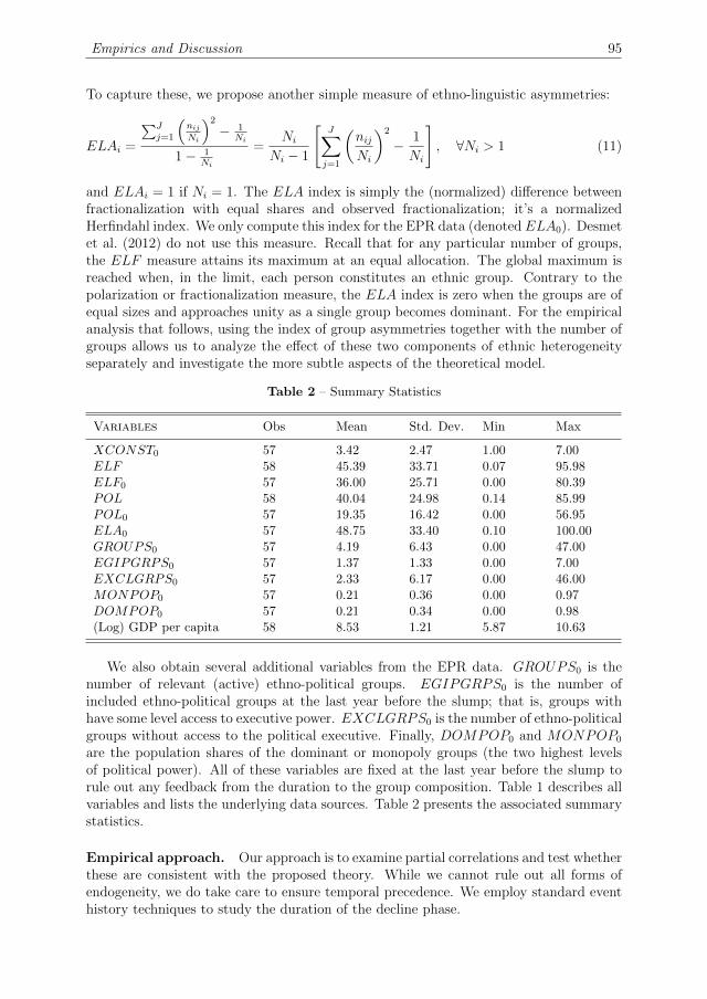
Empirics and Discussion 95
To capture these, we propose another simple measure of ethno-linguistic asymmetries:
ELAi =
∑Jj=1
(nijNi
)2
− 1Ni
1− 1Ni
=Ni
Ni − 1
[J∑
j=1
(nijNi
)2
− 1
Ni
], ∀Ni > 1 (11)
and ELAi = 1 if Ni = 1. The ELA index is simply the (normalized) difference betweenfractionalization with equal shares and observed fractionalization; it’s a normalizedHerfindahl index. We only compute this index for the EPR data (denoted ELA0). Desmetet al. (2012) do not use this measure. Recall that for any particular number of groups,the ELF measure attains its maximum at an equal allocation. The global maximum isreached when, in the limit, each person constitutes an ethnic group. Contrary to thepolarization or fractionalization measure, the ELA index is zero when the groups are ofequal sizes and approaches unity as a single group becomes dominant. For the empiricalanalysis that follows, using the index of group asymmetries together with the number ofgroups allows us to analyze the effect of these two components of ethnic heterogeneityseparately and investigate the more subtle aspects of the theoretical model.
Table 2 – Summary Statistics
Variables Obs Mean Std. Dev. Min Max
XCONST0 57 3.42 2.47 1.00 7.00ELF 58 45.39 33.71 0.07 95.98ELF0 57 36.00 25.71 0.00 80.39POL 58 40.04 24.98 0.14 85.99POL0 57 19.35 16.42 0.00 56.95ELA0 57 48.75 33.40 0.10 100.00GROUPS0 57 4.19 6.43 0.00 47.00EGIPGRPS0 57 1.37 1.33 0.00 7.00EXCLGRPS0 57 2.33 6.17 0.00 46.00MONPOP0 57 0.21 0.36 0.00 0.97DOMPOP0 57 0.21 0.34 0.00 0.98(Log) GDP per capita 58 8.53 1.21 5.87 10.63
We also obtain several additional variables from the EPR data. GROUPS0 is thenumber of relevant (active) ethno-political groups. EGIPGRPS0 is the number ofincluded ethno-political groups at the last year before the slump; that is, groups withhave some level access to executive power. EXCLGRPS0 is the number of ethno-politicalgroups without access to the political executive. Finally, DOMPOP0 and MONPOP0
are the population shares of the dominant or monopoly groups (the two highest levelsof political power). All of these variables are fixed at the last year before the slump torule out any feedback from the duration to the group composition. Table 1 describes allvariables and lists the underlying data sources. Table 2 presents the associated summarystatistics.
Empirical approach. Our approach is to examine partial correlations and test whetherthese are consistent with the proposed theory. While we cannot rule out all forms ofendogeneity, we do take care to ensure temporal precedence. We employ standard eventhistory techniques to study the duration of the decline phase.

96 Chapter 4. Ethnic divisions, political institutions and the duration of declines
To estimate the partial correlations, we run log-normal accelerated failure time (AFT)regressions of the form:
ln t ≡ ln(t− t0) =β0 + β1XCONST0 + β2H + β3(XCONST0 ×H) + x′0ξ + εt (12)
where t is analysis time, t0 is the last year before the slump, XCONST0 is executiveconstraints, H is a measure of group (ethnic) heterogeneity, x0 is a vector of controls,and εt ∼ N (0, σε). Variables which could endogenously react to a prolonged duration ofdeclines are kept fixed at t0 to rule out any such feedback; we drop the subscript if theyhave no time dimension. All parameters are estimated using Maximum Likelihood andthe standard errors are clustered on the country level to account for repeated spells.
Our main parameters of interest are β1, β2, and β3. In several regressions, we imposeβ3 = 0 to estimate first-order effects before examining a possible interaction effect. Thevector x0 may include additional heterogeneity measures, the (log of) initial GDP percapita before the slump, region effects and decade dummies.
Accelerated failure time models are so named due to their interpretation. A coefficientgreater than zero implies that time passes more slowly, so that the exit of the declinephase is prolonged. A coefficient less than zero implies that time passes more quicklyand hence that the recovery starts sooner. Alternatively, we may simply read the effectsas elasticities (or semi-elasticities) of the expected duration with respect to the variableson the right hand side. While duration models have the main benefit of accounting forunfinished spells (ongoing declines), their interpretation is otherwise identical to log-linearOLS when they are cast in the AFT form.
Results. Table 3 presents the first set of results relating mainly to the empiricalpredictions derived from the baseline model. We compute two sets of estimates. Oneusing the Ethnologue data which focuses on linguistic diversity and one based on the EPRdata which incorporates only politically-relevant groups divided along the predominantsocial cleavage (ethnic, linguistic, racial, etc.).
Columns (1) to (3) use the Ethnologue data. Column (1) establishes that strongerconstraints on the political executive shorten the expected duration of the decline phaseand that greater linguistic heterogeneity has an adverse effect on the expected duration.The effects are statistically significant at the 1%-level and economically meaningful. A onepoint improvement in executive constraints (before the slump) leads to an approximate18.7% reduction in the duration until the trough. Conversely, a one percentage pointchange towards greater linguistic heterogeneity prolongs the decline phase by about 1.7%.Column (2) allows for a conditional effect and strongly suggests that the effect of politicalinstitutions depends on the level of linguistic diversity (and vice versa). Whenever weintroduce an interaction term, we first center the two constituent variables on theiraverage. This shifts the coefficients of the two base levels into a meaningful range,but leaves the magnitude and statistical significance of the interaction term unaffected.Holding the other variable constant, the coefficient on either base variable now measuresthe effect of a one unit change away from the average. As a result, the interaction effectcan be ignored; it has to be taken into account only when both variables change. Theinteraction between executive constraints and linguistic fractionalization is significantat the 5%-level and comparatively large. The specification predicts that at perfecthomogeneity the median decline lasts about 2 years, while at perfect heterogeneity itlasts about 15 years. These estimates cover nearly all of the observed differences between

Empirics and Discussion 97
Table 3 – Baseline – Executive Constraints, Heterogeneity and Interactions
Dependent Variable: ln t
Variables (1) (2) (3) (4) (5) (6)
Ethnologue Ethnic Power Relations
XCONST0 -0.187*** -0.291*** -0.171*** -0.187*** -0.262*** -0.170**(0.063) (0.092) (0.064) (0.067) (0.085) (0.067)
ELF 0.017*** 0.019*** 0.023***(0.004) (0.004) (0.006)
ELF0 0.020*** 0.023*** 0.025***(0.007) (0.007) (0.007)
XCONST0×ELF15 -0.004**(0.002)
POL -0.011(0.007)
XCONST0 × ELF0 -0.004*(0.002)
POL0 0.012(0.009)
Control sets
GDP per capita Yes Yes Yes Yes Yes Yes
Summary stats
Exits 47 47 47 47 47 47Spells 57 57 57 57 57 57Years of Decline 346 346 346 346 346 346Log-L -73.677 -71.621 -72.679 -76.294 -74.952 -75.597Pseudo-R2 0.149 0.173 0.161 0.119 0.134 0.127
Note(s): The standard errors are clustered on the country level to account for repeated spells. Allspecifications include a constant (not shown). *** p<0.01, ** p<0.05, * p<0.1.
declines in Western Europe and Sub-Saharan Africa. The results in columns (1) and(2) are consistent with our theoretical predictions; greater constraints on the executiveshorten the expected duration unless the society is nearly homogeneous. The partialeffect of executive constraints is not statistically different from zero for low ELF values.Column (3) adds the linguistic polarization measure to the specification in column (1).The literature on civil conflict stresses that polarization matters; e.g. Esteban and Ray(2011) show theoretically that conflict over public goods is driven by polarization andconflict over private goods by fractionalization. Contrary to this literature but in linewith our model, we find no evidence in favor of the hypothesis that polarization is an issuefor (the lack of) cooperation during declines, while the coefficient on fractionalization isrobust to this perturbation. In other words, existence of two equally powerful groupsdoes not predict longer declines than, say, three equally-sized linguistic groups.
Measures of linguistic diversity tend to describe Sub-Saharan Africa as more diverse incomparison to other regions than alternative diversity measures. This begs the question

98 Chapter 4. Ethnic divisions, political institutions and the duration of declines
if we are just estimating an “Africa effect”. Columns (4) to (6) use the EPR data whichaddresses this issue by alternating the relevant cleavage by country (from racial overlinguistic to religious). This changes the relative location of Sub-Saharan Africa, whichis only the second most diverse region on this measure, after South Asia, contrary tobeing the most linguistically diverse region based on the Ethnologue data. The EPRdata also only codes politically relevant groups, so that the level of heterogeneity –no matter the measure – is generally lower. Note that we compute the heterogeneitymeasures for all politically relevant groups, not just the included groups. Strikingly,the results are virtually unchanged. Column (4) shows that the first order effects ofexecutive constraints are the same, and the effect of fractionalization is well within onestandard error of the previous estimate. Moreover, the sign and size of the interactioneffect in column (5) is nearly identical to the one in column (2). Only the statisticalsignificance of the interaction effect is a bit lower (cluster robust t-stat = -1.71). Column(5) shows that we also find no evidence in favor of ethno-political polarization affectingthe duration of declines, just as with linguistic polarization. Contrasting these resultsto the Ethnologue data, it seems safe to conclude that we are not only explaining thatdeclines in Sub-Saharan Africa last longer than elsewhere because the subcontinent is themost linguistically diverse, but that this holds try when we account for political relevanceand the prevalence of different divisions in different parts of the world.
Overall, Table 3 provides significant evidence that there is a robust partial correlationof the duration of the decline phase with executive constraints on the one hand and withethnic diversity on the other hand. In addition, the effect of weak constraints on theexecutive seems to be conditional on the degree of (ethno-political) fractionalization.
In Table 4 we “unpack” these statements further and examine what type of groupconfigurations give rise to the cooperation problem we are analyzing. These results relatemainly to the empirical content of the model extensions. We now only use the EPRdata, as it provides the necessary detail on the number of groups, their power statusand more. Column (1) presents a result that may appear puzzling at first sight. If wemeasure heterogeneity simply by the number of ethno-political groups, then we find noevidence of an effect on the duration of declines. However, this coefficient amalgamatestwo effects. The EPR data distinguishes between included groups, which have access toexecutive power, and excluded groups, which lack power at the state level or are (at worst)discriminated against. In the model presented earlier, only the former are relevant playersand thus we also expect that only the former category is empirically relevant. Column (2)confirms this expectation. The effect of included groups is statistically significant at the1%-level and economically very large: an additional group increases the duration of thedecline phase by about 53%. On the contrary, the effect of excluded groups is estimatedto be near zero and has a comparatively tight 99% confidence interval centered near zero.In line with the theory, these results suggest that only ethnic groups with some degree ofaccess to political power matter for the duration of declines.
We have not yet isolated whether this adverse effect of heterogeneity is due to severalequally powerful groups co-existing in society or due to particular asymmetries in politicalpower. Columns (3) to (6) represent different attempts towards empirically answeringthis question. In Comment 4, we translated the theoretical results regarding politicalconcentration from Proposition 3 and the number of groups from Proposition 4 intothe concepts of monopoly groups and dominant groups. Column (3) is the empiricalcounterpart. Here we relate the share of population represented by a group that eithermonopolizes or dominates the political executive to the duration of the decline phase.

Empirics and Discussion 99
Table 4 – Extensions – Number of Groups, Political Relevance, and Asymmetries
Dependent Variable: ln t
Variables (1) (2) (3) (4) (5) (6)
XCONST0 -0.225*** -0.241*** -0.215*** -0.179*** -0.210*** -0.200***(0.070) (0.063) (0.065) (0.066) (0.070) (0.073)
GROUPS0 -0.008 -0.031**(0.018) (0.014)
EGIPGRPS0 0.426*** 0.290** 0.300***(0.095) (0.124) (0.111)
EXCLGRPS0 -0.012 -0.021* -0.014(0.013) (0.012) (0.012)
DOMPOP0 -0.702*(0.361)
MONPOP0 -1.140**(0.484)
ELF0 0.022*** 0.013(0.007) (0.009)
ELA0 -0.013**(0.006)
Control sets
GDP per capita Yes Yes Yes Yes Yes Yes
Summary stats
Exits 47 47 47 47 47 43Spells 57 57 57 57 57 53Years of Decline 346 346 346 346 346 334Log-L -81.069 -75.062 -77.647 -75.457 -73.253 -66.669Pseudo-R2 0.064 0.133 0.103 0.129 0.154 0.166
Note(s): The standard errors are clustered on the country level to account for repeated spells. Allspecifications include a constant (not shown). *** p<0.01, ** p<0.05, * p<0.1.
The results are unambiguous. Both variables are associated with substantially shorterdeclines. Columns (4) and (5) try to explicitly tackle the issue of the number of groupsversus group asymmetries. In column (4), we include the number of ethno-politicallyrelevant group together with the index of ethno-political fractionalization. This leadsto an interesting ceteris paribus condition. Increasing the degree of fractionalization byone percentage point while holding constant the number of groups necessarily impliesthat political concentration is decreasing; that is, the groups are becoming more alike.Once again, recall that for any given number of groups, fractionalization is maximizedat equal shares. The estimates thus suggest that less political concentration leads tolonger declines. Column (5) again distinguishes between included and excluded groupsto illustrate that only the former are relevant. The coefficient on the ELF0 measureloses significance, suggesting that the number of included groups may drive the effectof ethnic heterogeneity and that group imbalances hardly matter. However, column(6) addresses this issue more directly by using our index of ethnic asymmetries and

100 Chapter 4. Ethnic divisions, political institutions and the duration of declines
provides the same answer as column (4). Now the effect is easy to interpret, negative andsignificant at the 5% level. A one percentage point move towards greater asymmetries(political concentration) shortens the duration by about 1.3%. Note that the effect ofexecutive constraints remains robust throughout, fluctuating around a 20% reduction inthe duration of declines for a one point improvement.
To summarize, Table 4 adds several valuable insights about the effect of ethnicdiversity on the duration of declines. Fractionalization of linguistic or ethno-politicalgroups masks two effects: 1) the expected duration is increasing in the number ofpolitically relevant groups, and 2) the expected duration is decreasing in greater groupasymmetries (political concentration). Both theory and evidence suggest that this is notan issue of polarization, but rather an issue of adding a smaller, potentially irrelevant,group to any multi-modal distribution of power as opposed to adding another powerfulgroup (an additional mode).
Table 5 – Robustness – Region and time effects
Dependent Variable: ln t
Variables (1) (2) (3) (4) (5) (6)
XCONST0 -0.245*** -0.216*** -0.211*** -0.171** -0.181*** -0.145**(0.079) (0.065) (0.077) (0.068) (0.066) (0.064)
ELF 0.020*** 0.021***(0.004) (0.003)
ELF0 0.017** 0.015**(0.007) (0.006)
XCONST0 × ELF -0.003** -0.004***(0.001) (0.001)
XCONST0 × ELF0 -0.003 -0.003*(0.002) (0.002)
EGIPGRPS0 0.298*** 0.212*(0.097) (0.119)
EXCLGRPS0 0.024* 0.009(0.013) (0.026)
Control sets
GDP per capita Yes Yes Yes Yes Yes YesRegional dummies Yes Yes Yes Yes Yes YesDecade dummies No Yes No Yes No Yes
Summary stats
Exits 47 47 47 47 47 47Spells 57 57 57 57 57 57Years of Decline 346 346 346 346 346 346Log-L -62.777 -55.812 -67.966 -64.108 -68.705 -66.701Pseudo-R2 0.275 0.355 0.215 0.260 0.207 0.230
Note(s): The standard errors are clustered on the country level to account for repeated spells. Allspecifications include a constant (not shown). *** p<0.01, ** p<0.05, * p<0.1.
Table 5 selects three key specifications, one for each data source, and then subjects

Concluding remarks 101
them to two robustness checks. First, we return to the issue of whether we are estimatingan “Africa effect” by including region dummies in each specification. Second, we controlfor temporal heterogeneity by including a dummy for the decade in which the slumpbegan in every other specification, since the 1970s, 1980s and 1990s exhibit significantlyhigher volatility than the other decades.
The Africa dummy is significant in all specifications, capturing that declines takesubstantially longer on the African continent. Nevertheless, we still find comparableeffects. Column (1) uses the Ethnologue data and shows that our two variables ofinterest are robustly correlated with within region differences in the duration of declines.Column (2) adds that this is still the case when we also control for temporal heterogeneity.Using the EPR data, columns (4) and (5) verify that the same holds for ethno-politicalfragmentation. The standard error of the interaction term becomes somewhat wider,leading to a loss of significance, but the estimated coefficient is extremely stable. The lasttwo columns show that this also hold for the effect of the number of included groups. Ingeneral, there is significant evidence of regional heterogeneity (a χ2-test always rejects thenull of no heterogeneity at the 5%-level), but there is somewhat less evidence of temporalheterogeneity (on top of duration dependence).8 Throughout Table 5 the coefficient ofpolitical institutions and the coefficients of the various measures of ethnic heterogeneityremain statistically significant at conventional levels and well within their usual range.
This last set of empirical findings reveals the following: first, ethnic heterogeneityand constraints on the political executive are robust determinants of the length of thedecline phase during major economic slumps. Second, this result is not due to regionaldifferences in ethnic heterogeneity but holds when we only use within region variation.Taken as a whole, we believe that these results operationalize the key parameters of themodel and demonstrate that there is robust evidence consistent with the theory outlinedhere.
6 Concluding remarks
This chapter presents a political economy theory of declines, highlighting a commitmentproblem between winners and losers of the recovery process after a crisis, and thenanalyzes empirical implications of this theory. We show that ethno-political heterogeneitycoupled with weak constraints on the political executive can bring about delayedcooperation during the decline phase of a slump and hence explain why we observe suchlong declines in some countries and relatively short declines in others.
Both the theory and the empirical analysis suggest that ethnic heterogeneity is indeedharmful for getting groups to agree on a response to a crisis when political institutions areweak. More subtle predictions show that this is mostly an issue of having many powerfulgroups in the society and does not apply to the same degree when there is a politicallydominant group. The overarching policy implication here is not that ethnic diversityis necessarily a problem, but that political institutions can be designed to contain theadversarial element of ethnic heterogeneity in particular and political heterogeneity ingeneral. While not restricted to understanding declines in Sub-Saharan Africa, we wouldlike to once again emphasize that we believe these insights are particularly importantfor understanding the political economy of declines on the subcontinent. Sub-Saharan
8A χ2-test rejects the null of no temporal heterogeneity at the 1%-level in column (1), at the 5%-levelbut not the 1%-level in column (4), and fails to reject the null at conventional levels in column (6).

102 Chapter 4. Ethnic divisions, political institutions and the duration of declines
Africa is home to the longest and deepest declines, politics shaped by ethnicity, and weakinstitutions governing executive power. While we still need to better understand whyethnic diversity tends to coincide with weak political institutions and how one shapes theother, we find that there is ample room for managing this heterogeneity better so thatwelfare gains are not lost in the next crisis.
This line of research is far from complete. Fruitful avenues for future research would beto extend these models further by integrating a richer description of the executive decision-making process, altering the decision rules, treating the quality of political institutions asendogenous to the decline, or modeling details of the policy response. On the empiricalside, richer data on cabinet allocations, ethnicity and executive power would help to traceout the proposed mechanism more carefully.

Bibliography 103
Bibliography
Acemoglu, D. and J. A. Robinson (2006). Economic Origins of Democracy and Dictatorship. CambridgeUniversity Press.
Aghion, P., A. Alesina, and F. Trebbi (2004). Endogenous political institutions. Quarterly Journal ofEconomics 119 (2), 565–611.
Ahlerup, P. and O. Olsson (2012). The roots of ethnic diversity. Journal of Economic Growth 17 (2),71–102.
Alesina, A., R. Baqir, and W. Easterly (1999). Public goods and ethnic divisions. Quarterly Journal ofEconomics 114 (4), 1243–1284.
Alesina, A. and A. Drazen (1991). Why are stabilizations delayed? American Economic Review 81 (5),1170–1188.
Alesina, A. and E. L. Ferrara (2005). Ethnic diversity and economic performance. Journal of EconomicLiterature 43 (3), 762–800.
Alesina, A., C. Gennaioli, and S. Lovo (2014, September). Public goods and ethnic diversity: Evidencefrom deforestation in Indonesia. Working Paper 20504, National Bureau of Economic Research.
Alesina, A. F., S. Michalopoulos, and E. Papaioannou (2012, November). Ethnic inequality. WorkingPaper 18512, National Bureau of Economic Research.
Ashraf, Q. and O. Galor (2013). The “Out of Africa” hypothesis, human genetic diversity, andcomparative economic development. American Economic Review 103 (1), 1–46.
Bates, R. H. (2000). Ethnicity and development in Africa: A reappraisal. American EconomicReview 90 (2), 131–134.
Berg, A., J. D. Ostry, and J. Zettelmeyer (2012). What makes growth sustained? Journal of DevelopmentEconomics 98 (2), 149–166.
Besley, T. and T. Persson (2011a). Fragile states and development policy. Journal of the EuropeanEconomic Association 9 (3), 371–398.
Besley, T. and T. Persson (2011b). The logic of political violence. Quarterly Journal of Economics 126 (3),1411–1445.
Bueno de Mesquita, B., A. Smith, and R. M. Siverson (2005). The logic of political survival. MIT press.
Caselli, F. and W. J. Coleman (2013). On the theory of ethnic conflict. Journal of the European EconomicAssociation 11, 161–192.
Cederman, L.-E., A. Wimmer, and B. Min (2010). Why do ethnic groups rebel? New data and analysis.World Politics 62 (1), 87–119.
Cerra, V. and S. C. Saxena (2008). Growth dynamics: The myth of economic recovery. AmericanEconomic Review 98 (1), 439–57.
Collier, P. (2000). Ethnicity, politics and economic performance. Economics & Politics 12 (3), 225–245.
Cox, G. W. and M. D. McCubbins (1997). Political structure and economic policy: The institutionaldeterminants of policy outcomes. In S. Haggard and M. D. McCubbins (Eds.), Presidents, Parliaments,and Policy, pp. 21–63. Cambridge University Press.
Desmet, K., I. Ortuno-Ortın, and R. Wacziarg (2012). The political economy of linguistic cleavages.Journal of Development Economics 97 (2), 322–338.
Drazen, A. and V. Grilli (1993). The benefit of crises for economic reforms. American EconomicReview 83 (3), 598–607.
Easterly, W. (2001). Can institutions resolve ethnic conflict? Economic Development and CulturalChange 49 (4), 687–706.
Easterly, W., M. Kremer, L. Pritchett, and L. Summers (1993). Good policy or good luck? Journal ofMonetary Economics 32 (3), 459–483.
Easterly, W. and R. Levine (1997). Africa’s growth tragedy: Policies and ethnic divisions. QuarterlyJournal of Economics 112 (4), 1203–1250.
Eifert, B., E. Miguel, and D. N. Posner (2010). Political competition and ethnic identification in Africa.American Journal of Political Science 54 (2), 494–510.
Esteban, J., L. Mayoral, and D. Ray (2012). Ethnicity and conflict: An empirical study. AmericanEconomic Review 102 (4), 1310–1342.
Esteban, J. and D. Ray (1994). On the measurement of polarization. Econometrica 62 (4), 819–851.
Esteban, J. and D. Ray (2011). Linking conflict to inequality and polarization. American EconomicReview 101 (4), 1345–1374.

104 Bibliography
Fearon, J. D. (2003). Ethnic and cultural diversity by country. Journal of Economic Growth 8 (2),195–222.
Fearon, J. D. and D. D. Laitin (2003). Ethnicity, insurgency, and civil war. American Political ScienceReview 97, 75–90.
Fernandez, R. and D. Rodrik (1991). Resistance to reform: Status quo bias in the presence of individual-specific uncertainty. American Economic Review 81 (5), 1146–1155.
Francois, P., I. Rainer, and F. Trebbi (2012, September). How is power shared in Africa? Working Paper18425, National Bureau of Economic Research.
Gehlbach, S. and E. J. Malesky (2010). The contribution of veto players to economic reform. The Journalof Politics 72 (4), 957–975.
Haggard, S. (2000). The political economy of the Asian financial crisis. Peterson Institute forInternational Economics.
Hausmann, R., L. Pritchett, and D. Rodrik (2005). Growth accelerations. Journal of EconomicGrowth 10 (4), 303–329.
Hicken, A., S. Satyanath, and E. Sergenti (2005). Political institutions and economic performance: Theeffects of accountability and obstacles to policy change. American Journal of Political Science 49 (4),897–907.
Laban, R. and F. Sturzenegger (1994a). Distributional conflict, financial adaptation and delayedstabilizations. Economics & Politics 6 (3), 257–276.
Laban, R. and F. Sturzenegger (1994b). Fiscal conservatism as a response to the debt crisis. Journal ofDevelopment Economics 45 (2), 305 – 324.
Michalopoulos, S. (2012). The origins of ethnolinguistic diversity. American Economic Review 102 (4),1508–39.
Miguel, E. and M. K. Gugerty (2005). Ethnic diversity, social sanctions, and public goods in Kenya.Journal of Public Economics 89 (11–12), 2325–2368.
Posner, D. N. (2004). Measuring ethnic fractionalization in Africa. American Journal of PoliticalScience 48 (4), 849–863.
Rainer, I. and F. Trebbi (2012, September). New tools for the analysis of political power in Africa.Working Paper 18424, National Bureau of Economic Research.
Rodrik, D. (1999). Where did all the growth go? External shocks, social conflict, and growth collapses.Journal of Economic Growth 4 (4), 385–412.
Spolaore, E. (2004). Adjustments in different government systems. Economics & Politics 16 (2), 117–146.
Tsebelis, G. (1995). Decision making in political systems: Veto players in presidentialism,parliamentarism, multicameralism and multipartyism. British Journal of Political Science 25 (03),289–325.
Tsebelis, G. (2002). Veto players: How political institutions work. Princeton University Press.
Wimmer, A., L.-E. Cederman, and B. Min (2009). Ethnic politics and armed conflict: A configurationalanalysis of a new global data set. American Sociological Review 74 (2), 316–337.

Appendix 105
Appendix: Proofs
Proof of Proposition 1. The utility from cooperation in the first period when theother group cooperates is
v1j (C, c) =
1
1− δ (1− 2c)E[g(wj)|wj ∈ A] + c(g(0) + g(1)) (A-1)
and the utility from choosing to delay cooperation one period when the other groupcooperates is
v1j (D, c) =g((1−∆)yj) +
δ
1− δ
(1− 2p2)E[g(wj)|wj ∈ A] + p2(g(0) + g(1))
(A-2)
where p2 = c − x; that is, half the probability of landing outside the safe zone in thesecond period.
The proof is by contradiction. We conjecture an equilibrium with immediate recovery,such that v1
j (C, c) ≥ v1j (D, c). Using p2 = c− x and rearranging terms, we get
g((1−∆)yj) ≤
E[g(wj)|wj ∈ A]−[c+
δ
1− δx]2E[g(wj)|wj ∈ A]− g(0)− g(1) . (A-3)
Note that concavity implies that 2E[g(wj)|wj ∈ A]− g(0)− g(1) > 0. Inequality (A-3)is contradicted whenever c, x or δ are large enough in relation to ∆, depending on theshape of the utility function g(yj) and its range, which completes the proof.
Proof of Proposition 2. First of all, it is useful to demonstrate that the differencein utility between recovery at any time period (t) and recovery at the subsequent period(t+ 1) decreases over time. For all s > t, we need to check whether
vt+1j (C, c)− vtj(C, c) > vs+1
j (C, c)− vsj (C, c). (A-4)
Note that vt+1j (C, c) = vtj(D, c).
Substituting the utilities and rearranging the inequality, we get
g((1−∆)yj)− (1− 2pt)E[g(wj)|wj ∈ A]− pt(g(0) + g(1))+
δ
1− δ
2(pt − pt+1)E[g(wj)|wj ∈ A] + (pt+1 − pt)(g(0) + g(1))>
g((1−∆)yj)− (1− 2ps)E[g(wj)|wj ∈ A]− ps(g(0) + g(1))+
δ
1− δ
2(ps − ps+1)E[g(wj)|wj ∈ A] + (ps+1 − ps)(g(0) + g(1)).
(A-5)
Recall that pt = c− (t− 1)x implies pt+1− pt = −x, so the second and third terms canceland the inequality reduces to
(1− 2pt)E[g(wj)|wj ∈ A] + pt(g(0) + g(1)) <
(1− 2ps)E[g(wj)|wj ∈ A] + ps(g(0) + g(1)).(A-6)
Substituting pt = c− (t− 1)x again, it is straightforward to show that this inequality is

106 Appendix
always satisfied when s > t.
Having established this, setting the utility of choosing to cooperate in period t equalto the utility of recovering in period t + 1 results in an equation that will deliver apotentially non-integer t, such that the smallest higher integer (dte) is the equilibriumtime to recovery:
1
1− δ
(1− 2pt)E[g(wj)|wj ∈ A] + pt(g(0) + g(1))
= g((1−∆)yj)+
δ
1− δ
(1− 2pt+1)E[g(wj)|wj ∈ A] + pt+1(g(0) + g(1)).
(A-7)
Inserting the linear process on pt = c− (t− 1)x yields
1
1− δ (1− 2(c− (t− 1)x))E[g(wj)|wj ∈ A] + (c− (t− 1)x)(g(0) + g(1)) =
g((1−∆)yj) +δ
1− δ (1− 2(c− tx))E[g(wj)|wj ∈ A] + (c− tx)(g(0) + g(1)) .(A-8)
Isolating the first term of the geometric series gives
(1− 2(c− (t− 1)x))E[g(wj)|wj ∈ A] + (c− (t− 1)x)(g(0) + g(1))+
δ
1− δ (1− 2(c− (t− 1)x))E[g(wj)|wj ∈ A] + (c− (t− 1)x)(g(0) + g(1)) =
g((1−∆)yj) +δ
1− δ (1− 2(c− tx))E[g(wj)|wj ∈ A] + (c− tx)(g(0) + g(1))
(A-9)
and after canceling the common terms, we have
(1− 2c)E[g(wj)|wj ∈ A] + c(g(0) + g(1))+
tx2E[g(wj)|wj ∈ A]− (g(0) + g(1))
= g((1−∆)yj) +1
1− δx 2E[g(wj)|wj ∈ A]− (g(0) + g(1)) .(A-10)
Solving for t∗ and simplifying gives
t∗ =g((1−∆)yj)− E[g(wj)|wj ∈ A]
x2E[g(wj)|wj ∈ A]− (g(0) + g(1)) +c
x+
1
1− δ . (A-11)
The proposition follows directly from comparative statics w.r.t. to c
∂t∗
∂c=
1
x> 0 (A-12)
that is, stronger executive constraints (smaller c) shorten the time to cooperation. Thiscompletes the proof for the interior case. Note that it can also be the case that recoveryhappens at the point when all uncertainty is resolved, i.e. the point where the probabilityof being outside the safe zone is zero and no longer changes. If this is the case it isstraightforward to see that the time to recovery is shorter with stronger constraints on theexecutive. This follows directly from the fact, that the time it takes until all uncertaintyis resolved is shorter with smaller c.

Appendix 107
Proof of Proposition 3. Recall that for the asymmetric case only one group risksfalling outside the political safe zone. Hence, for there to exist an equilibrium withrecovery in the first period, the following condition needs to be true
1
1− δ (1− p1(yj))yj + p1(yj)z ≥ (1−∆)yj +δ
1− δ yj (A-13)
which simplifies to
∆yj +1
1− δ p1(yj)(z − yj) ≥ 0. (A-14)
An decrease in concentration (asymmetry) makes delay more likely if the left hand sideof the inequality is a decreasing function of yj. This is true when the derivative of theleft hand side is negative:
∆ +1
1− δ
dp1(yj)
dyj(z − yj)− p1(yj)
< 0 (A-15)
which completes the proof.
Proof of Proposition 4. Remember that there always exists an equilibrium withrecovery in period two in the sub-game that starts in period two after delay in periodone. If all of the other groups decide to cooperate in period 1, it is optimal for theremaining group to cooperate if the following condition holds
1
1− δ
(1− Jp1(yj))
1
J+ (J − 1)p1(yj)
(1
J+
1
(J − 1)J
)+ p1(yj)z
≥
(1−∆)1
J+
δ
1− δ1
J.
(A-16)
The second term inside the curly braces simplifies to pt(yj), so that inequality (A-16)becomes
1
1− δ
(1− Jp1(yj))
1
J+ p1(yj) + p1(yj)z
≥ (1−∆)
1
J+
δ
1− δ1
J(A-17)
or
1
1− δ
1
J+ p1(yj)z
≥ (1−∆)
1
J+
δ
1− δ1
J(A-18)
and, after some algebraic manipulation, this simplifies to
∆
J+
1
1− δp1(yj)z ≥ 0. (A-19)
Note that p1(yj) is increasing in J , as symmetry implies yj = 1/J , and z < 0 by definition.As a result, the inequality becomes harder to satisfy if the number of groups increases,which completes the proof.


Part II
Growth, distribution and poverty


Chapter 5
The pace of poverty reduction
A fractional response approach∗
Abstract
The pace of poverty reduction through growth v. redistribution is atthe heart of current debates on equitable development. In this chapter, weargue that empirical poverty decompositions should build in the inherentboundedness of the poverty headcount ratio directly. As a solution, wepropose a fractional response approach to estimating poverty decompositions,and present extensions dealing with unobserved heterogeneity, measurementerror and unbalancedness. Using a large new data set, we estimate incomeand inequality (semi-)elasticities of poverty for the $2 a day and $1.25 a daypoverty lines. The models fit the data remarkably well over the entire datarange. We highlight the relevance of focusing on semi-elasticities for policypurposes and, building on the improved accuracy of the fractional responseresults, we present poverty projections from 2010 through 2030. Finally,we discuss some implications of these results for the post-2015 developmentagenda.
Keywords: poverty, inequality, fractional response models, income growth
JEL Classification: I32, C25, O10, O15
∗This chapter is based on Bluhm, R., de Crombrugghe, D., and A. Szirmai. 2013. The pace of povertyreduction - A fractional response approach,” MERIT Working Papers 051, United Nations University -Maastricht Economic and Social Research Institute on Innovation and Technology (MERIT).
111

112 Chapter 5. The pace of poverty reduction
1 Introduction
The pace of poverty reduction through economic growth is at the heart of ongoing debateson inclusive growth and equitable development. Given the salience of this issue to bothpolicy makers and academics, an increasingly large literature analyzes the impact ofchanges in incomes and inequality on poverty, as well as their respective contributionstowards poverty reduction in the past decades (Ravallion and Chen, 1997; Besley andBurgess, 2003; Bourguignon, 2003; Kraay, 2006; Kalwij and Verschoor, 2007; Bresson,2009; Chambers and Dhongde, 2011). Collectively, these studies established not only thatincome growth is crucial to achieving sustained decreases in poverty but also that thebenefits of income growth strongly depend on the initial levels of income and inequality.In fact, poverty is linked to income and distribution through a decomposition identitythat should guide empirical studies of poverty (Datt and Ravallion, 1992; Kakwani, 1993;Bourguignon, 2003). In this chapter, we revisit and extend this literature in several ways.
First, and most fundamentally, we argue that the previous literature based on linearmodels of poverty changes ignores the bounded nature of the poverty headcount ratioand either disregards or awkwardly reintroduces the information provided by incomeand inequality levels. This leads to poorly fitting approximations of the underlyingdecomposition identity and estimates of the relevant elasticities that can take onimplausible values. Instead, we propose that empirical models of poverty should capturethe boundedness of the poverty headcount ratio directly, and thus build in the inherentnon-linearity of the relationship and the non-constancy of the elasticities. To this end, wederive fractional response models of the poverty headcount ratio. We present extensions ofthese models that deal with unobserved heterogeneity, measurement error and unbalancedpanel data (see Papke and Wooldridge, 1996, 2008; Wooldridge, 2010a). A key result isthe greatly improved accuracy of the poverty decomposition. Our specifications fit thedata remarkably well and predict the observed poverty headcount ratio with less than 2.5percentage points error on average. For comparison, we also reproduce the traditionalapproach and highlight some of its empirical shortcomings.
Second, using a new data set of 809 nationally representative surveys covering 124countries from 1981 to 2010, we estimate income and inequality elasticities of the povertyheadcount ratio for different regions and time periods. Our findings generally confirmthe result of previous studies that the average income elasticity of poverty is aroundtwo. However, in order to understand the speed of poverty reduction across differentregions and time periods, we are particularly interested in reliable estimates of valuesother than the overall cross-country mean. Our method provides considerably moreprecise regional and temporal estimates of the income and inequality elasticities of povertythat often contradict earlier studies. For example, we find universally higher incomeelasticities in Latin America and Eastern Europe and Central Asia but lower incomeelasticities in both South Asia and Sub-Saharan Africa than reported earlier (Kalwijand Verschoor, 2007). Furthermore, since income or inequality elasticities of poverty areconcepts of relative change, they may give the misleading impression that richer countriesare becoming ever better at reducing poverty even though the underlying absolute changesare small. Hence, we also stress the importance of semi-elasticities which capture theabsolute change in poverty for a given rate of income growth or proportional change inthe income distribution (Klasen and Misselhorn, 2008).
Last but not least, based on the much improved accuracy of our new estimates, wepresent projections of the poverty headcount ratio for the $2 a day and $1.25 a day poverty

Modeling poverty and elasticities 113
lines until 2030. We find that absolute poverty in Sub-Saharan Africa and, as a not toodistant second, South Asia remains the primary development challenge of the twenty-firstcentury. In all other regions, poverty is projected to nearly disappear or fall to much lessthan 10% of the population by 2030. These results are based on the assumption thatper capita incomes and expenditures in each country continue to grow at the averagepace of the last 15 years. While it is clearly far from guaranteed that this will hold true,other assumptions are easily evaluated using our proposed estimation framework. Theprojected poverty trends have direct bearing on the post-2015 development agenda andcan be used to assess the viability of proposed development goals.
The remainder of this chapter is organized as follows. Section 2 reviews how theexisting literature models poverty, derives our approach, and discusses the econometricsof fractional response models. Section 3 briefly outlines the data used in this chapter.Section 4 presents the estimation results, regional elasticities, and poverty projectionsuntil 2030. Section 5 concludes.
2 Modeling poverty and elasticities
2.1 Traditional approaches: linear models of poverty changes
Using micro-data, changes in poverty can be decomposed into changes in income and theincome distribution up to some error (Datt and Ravallion, 1992; Kakwani, 1993). A keyproblem for cross-country studies of poverty is that we generally do not have access tomicro data sets of incomes and/or consumption expenditures for all countries but usuallyestimate poverty based on grouped data.1 To overcome this limitation, Bourguignon(2003) suggests approximating the entire income distribution of each country using atwo-parameter log normal distribution – an approach that is theoretically grounded2,simple and popular but not without its critics (e.g. Bresson, 2009).
Bourguignon assumes that income, yt, is a log normal random variable, such thatln yt ∼ N (µt, σ
2t ), and mean income can be written as yt = E[yt] = exp(µt + σ2
t /2). Thenthe poverty headcount ratio (henceforth, poverty headcount) at time t may be defined as
Ht = H(yt/z, σt) = Φ
(− ln(yt/z)
σt+
1
2σt
)≡ Pr[yt ≤ z] (1)
where Φ(·) denotes the standard normal cdf, inequality is measured as the standarddeviation (σt) of log income, and yt/z is the (relative) distance of mean income (yt) tothe (fixed) poverty line (z) – which we interpret as a ‘shortfall’ when yt < z and ‘affluence’when yt > z.
1There have been some attempts to either collect all the available primary data or to estimate gapsin survey coverage with the help of national accounts. Milanovic (2002) compiles a global data setof household level data to study the evolution of inequality, Sala-i-Martin (2006) estimates a “worldincome distribution” via kernel density approximations based on grouped data, and Kraay (2006) fitsthree-parameter Lorenz curves to grouped data in order to estimate the entire income distribution forthe country-poverty spells in his sample.
2Gibrat’s law, for example, illustrates how the log normal distribution can arise from a sequence ofstochastic income shocks ln yt = ln yt−1 + et, so that et is a random transitory shock in log income andas t grows the distribution of et defines the distribution of ln yt. Battistin, Blundell, and Lewbel (2009)recently argued that this process is better thought of in terms of permanent income and suggest thatconsumption is closer to a log normal distribution.

114 Chapter 5. The pace of poverty reduction
Eq. (1) can be interpreted as the probability that, at a particular time t, an individualrandomly drawn from the population is poor. This formulation gave rise to a largeliterature deriving the income and inequality elasticities of poverty analytically andestimating econometric models inspired by their analytic counterparts (e.g. Bourguignon,2003; Kalwij and Verschoor, 2007; Klasen and Misselhorn, 2008). To summarize theessence of this approach note that, based on eq. (1), we can derive the income elasticity(εHyt = ∂Ht
∂yt
ytHt
) and inequality elasticity (εHσt = ∂Ht∂σt
σtHt
) of the poverty headcount as
εHyt = − 1
σtλ
(− ln(yt/z)
σt+
1
2σt
)(2)
and
εHσt =
(ln(yt/z)
σt+
1
2σt
)λ
(− ln(yt/z)
σt+
1
2σt
)(3)
where we define the inverse Mills ratio (λ(x) ≡ φ(x)/Φ(x)) as the ratio of the standardnormal pdf to the standard normal cdf, and we require Ht > 0.
The decomposition of the poverty headcount is often written as
dHt
Ht
≈ εHytdytyt
+ εHσtdσtσt
(4)
where dHt/Ht is a small relative change in the poverty headcount, dyt/yt is a smallrelative change in mean incomes, and dσt/σt is a small relative change in the standarddeviation of log incomes. The approximation follows from a linear Taylor expansion ofHt. Appendix A derives this result.3
Given log normality, the standard deviation is a monotone transformation of the Giniinequality coefficient, denoted Gt, and can be obtained via σt =
√2Φ−1(Gt/2+1/2).4 So,
eqs. (2) and (3) can be used to predict the elasticities directly using observed values ofincome and inequality. With some additional algebra, we can also derive an expressionfor the Gini elasticity and rewrite eq. (4) accordingly – see eq. (A-6) in Appendix A.
However, the assumption of log normality is only an approximation and unlikelyto hold exactly. The key observation motivating the econometric models is that bothelasticities depend only on the initial levels of mean income and inequality (when thepoverty line is fixed). In order to allow for misspecification of the functional form, theauthors rely on a linear approximation of these intrinsically non-linear functions. Theycapture the dependence on initial levels by interacting both mean income and inequalitywith the ratio of initial mean income to the poverty line and with initial inequality. Thismodel is sometimes called the “improved standard model” (Bourguignon, 2003) and it isusually formulated in (annualized) differences:
∆ lnHit = α + β1∆ ln yit + β2∆ ln yit × ln(yi,t−1/z) + β3∆ ln yit × lnGi,t−1
+ γ1∆ lnGit + γ2∆ lnGit × ln(yi,t−1/z) + γ3∆ lnGit × lnGi,t−1 + εit(5)
where ∆ is the difference operator, α is a linear time trend and εit is an error term. Wealso added country subscripts.
3Also see Datt and Ravallion (1992), Kakwani (1993) and Bourguignon (2003).4This formulation is the inverse of Gt = 2Φ(σt/
√2)− 1 due to Aitchison and Brown (1957).

Modeling poverty and elasticities 115
Suppose eq. (5) is estimated via OLS or GMM, then it is straightforward to see thatthe implied elasticities approximate eqs. (2) and (3). The estimated income elasticity isεHyit = β1+β2 ln(yi,t−1/z)+β3 lnGi,t−1 and the estimated inequality elasticity is εHGit = γ1+γ2 ln(yi,t−1/z) + γ3 lnGi,t−1. Clearly, the elasticities depend on the initial levels of incomeand inequality. These two elasticities are sometimes referred to as the ‘distribution-neutral’ income elasticity and the ‘growth-neutral’ inequality elasticity. They identifythe partial effect of changing either income or inequality, contrary to the simple observedelasticity that confounds both effects.5 Yet, this approximation is extremely coarse anddoes not place any meaningful restrictions on the parameter space. Moreover, it is unclearwhich level equation this specification derives from.
In general, poverty elasticities can paint a distorted picture of poverty dynamics. Theincome elasticity, for example, gives the impression that richer countries become everbetter at poverty reduction because a drop in the poverty headcount from 2% to 1% istreated just the same as a drop from 50% to 25%. Recognizing this shortcoming, Klasenand Misselhorn (2008) suggest to focus on absolute poverty changes instead. Removingthe log from the headcount in eq. (5) turns it into a model of semi-elasticities and altersthe interpretation.6 The coefficients now measure the percentage point change in thepopulation that is below the poverty line for a given rate of change in income or inequality.Likewise, eqs. (2) and (3) can be written as semi-elasticities by replacing the inverse Millsratio with the standard normal pdf. Contrary to elasticities, the semi-elasticities approachzero as mean income becomes large. Klasen and Misselhorn (2008) also report that theirmodels fit the data better and suggest that the specification in absolute changes capturesmore of the inherent non-linearity. Nevertheless, given the underlying identity, the fittypically found in the literature (.55 ≤ R2 ≤ .73) is not particularly high.
There are advantages to relying on a linear framework other than mere simplicity,such as the well-known robustness properties of popular estimators. Nevertheless, aspecification like eq. (5) suffers from several problems. First, it completely disregards theinformation provided by poverty levels, most likely introduces negative serial correlation,and compounds pre-existing measurement error.7 Second, after differencing removes thetime-constant unobserved effects, the added interaction terms reintroduce the unobservedeffects present in the lagged levels. Hence, the coefficients are likely to be biased nomatter if the model is estimated using Ordinary Least Squares (OLS), InstrumentalVariables (IV) or Generalized Methods of Moments (GMM) if time invariant measurementdifferences exist.8 Third and most fundamentally, the intrinsic non-linearity of the (semi-)elasticities is due to the bounded nature of the dependent variable which is not taken intoaccount by linear specifications. The poverty headcount is a proportion and thus onlytakes on values in the unit interval (Hit ∈ [0, 1]). As a result, the linear estimates are
5For recent estimates of the simple empirical elasticity (d lnHit/d ln rgdpcit, where rgdpcit is realGDP per capita), see Ram (2013).
6The term semi-elasticity refers here to the quantity ∂y∂ ln x = ∂y
∂xx rather than the more usual ∂ ln y∂x =
∂y∂x
1y .7If the errors in the original process (say, yit = α + β(xit + νit) + εit, where νit is a mean zero
process uncorrelated with xit ) are not autocorrelated, then differencing introduces correlation: ∆εit hasa term in common with ∆εi,t−1, so E[∆εit∆εi,t−1] = E[−ε2i,t−1] = −σ2
ε . Furthermore, any attenuation
bias is magnified by the first-difference transformation: plim(βFD) = βσ2∆x/(σ
2∆x +σ2
∆ν) where typicallyσ2
∆ν = 2σ2ν but σ2
∆x < 2σ2x. Autocorrelation in the mismeasured variables further reduces the signal to
noise ratio and increases the attenuation bias.8Cf. Kalwij and Verschoor (2007), who first show a simpler linear model in differences to remove the
unobserved effects and then estimate interaction models with unobserved effects reintroduced.

116 Chapter 5. The pace of poverty reduction
unlikely to work well for values distant from the mean and can easily take on implausiblevalues (e.g. εHyit > 0) for some combinations of income and inequality. Any version of thelinear model will only poorly approximate the non-linear shape. Yet for these estimatesto be relevant for any particular country or region, we are precisely interested in temporaland/or regional elasticities and not just the overall cross-country mean elasticities.
2.2 Alternative approaches: non-linear models of poverty
We propose modeling the conditional expectation of the poverty headcount using non-linear parametric fractional response models. To the best of our knowledge, we are thefirst to use such an approach for estimating poverty elasticities.
Some weaknesses of the linear specifications have been highlighted before. Chambersand Dhongde (2011) argue that the functional form is the source of the non-linearity.They estimate non-parametric models of the conditional mean of the headcount (Hit =m(yit, Git)+εit) and then obtain average elasticities. However, non-parametric techniquesare often inefficient, cannot handle many covariates (due to the curse of dimensionality),and cannot easily deal with measurement error. It is generally difficult to test moreinvolved hypotheses in a non-parametric framework. Nevertheless, we fully agree withChambers and Dhongde (2011) that non-linear estimation of the conditional meanmatters.
We follow Papke and Wooldridge (1996), who first suggested modeling proportionsusing fractional logit or fractional probit to estimate models of the form E[yi|xi] = F (x′iβ),where yi ∈ [0, 1] and F (·) is the logistic or normal cdf. Applying this approach to ourproblem, we may approximate eq. (1) with
E[Hit|yit, Git] = Φ(α + β ln yit + γ lnGit) for i = 1, . . . , N ; t = 1, . . . , T (6)
where ln z is absorbed into the constant and we also take the logarithm of the Ginicoefficient (mostly for convenience). Naturally, we expect β < 0 and γ > 0. In motivatingthis model, we temporarily assume away all econometric complications such as unobservedheterogeneity, endogeneity and unbalancedness. These assumptions are relaxed in thenext subsection.
Since F (·) is invertible, it can be used as a ‘link function’ in the spirit of the GLMliterature (e.g. MacCullagh and Nelder, 1989). Thus, we may also write eq. (6) asΦ−1 (E[Hit|yit, Git]) = α + β ln yit + γ lnGit. In other words, the inverse normal cdflinearizes the conditional mean. Figures B-1 and B-2 in Appendix B use this propertyto plot Φ−1(Hit) against ln yit and lnGit for each region, including a regression line. Theresult is striking. This simple transformation is extremely successful in removing theintrinsic non-linearity of the poverty headcount.
It is now straightforward to define the estimated income elasticity as
εHyit =∂E[Hit|yit, Git]
∂yit
yit
E[Hit|yit, Git]= β × λ
(α + β ln yit + γ lnGit
)(7)
and the estimated Gini elasticity as
εHGit =∂E[Hit|yit, Git]
∂Git
Git
E[Hit|yit, Git]= γ × λ
(α + β ln yit + γ lnGit
). (8)

Modeling poverty and elasticities 117
Contrary to the linear model, the elasticities in eqs. 7 and 8 closely mimic theproperties and structure of the analytical elasticities in eqs. 2 and 3. The non-linearityarises simply from the bounded functional form and is not artificially captured byinteraction terms. However, it is important to note that we do not require log normalitybut implicitly assume that an unspecified two-parameter distribution sufficiently describesthe poverty headcount up to statistical error. We simply derived a more natural modelof the poverty headcount as a function of income and inequality which happens to looka lot like its theoretical counterpart.
This approach has several advantages. We directly take the information provided bypoverty levels into account, the model predictions of the poverty headcount ratio willstrictly lie in the unit interval, and the same model is able to estimate both elasticitiesand semi-elasticities. As a result of respecting the bounded nature of the headcount, theelasticities will also approach zero when the inverse Mills ratio becomes vanishingly smalland are likely to closely approximate values further away from the mean of the covariates.Hence, they share important properties of their theoretical counterparts based on the lognormal assumption. Furthermore, we can directly predict the poverty headcount forinteresting combinations of income and inequality rather than going the roundabout wayof estimating the elasticities in one model and then projecting poverty separately.
2.3 Econometrics of fractional response models
Since there is no free lunch in econometrics, the apparent gains over the linear approachmust come at a price. In non-linear models it is generally harder to deal with unobservedheterogeneity, measurement error and unbalancedness. While until a few years agothere was relatively little research on this issue, we can now draw on an increasinglywell developed framework. Papke and Wooldridge (2008) extend fractional responsemodels to balanced panels with unobserved heterogeneity and endogenous covariates,Wooldridge (2010a) develops the theory for unbalanced panels, and Wooldridge (2012)derives a general set-up for one-step estimators in non-linear models. Other contributionsto the field are Loudermilk (2007), Cook, Kieschnick, and McCullough (2008), Ramalho,Ramalho, and Murteira (2011), and Tiwari and Palm (2011).
To simplify the exposition, we stack the coefficients β = (β1, β2, . . . , βk)′ and covariates
xit = (xit,1, xit,2, . . . , xit,k)′. The ideal model we would like to estimate is
E[Hit|xi, µi] = E[Hit|xit, µi] = Φ(x′itβ + µi) for i = 1, . . . , N ; t = 1, . . . , T (9)
where xi = (xi1,xi2, . . . ,xiT ) are the covariates in all periods. We assume that thecovariates are strictly exogenous conditionally on the unobserved effects (µi), and thatthe panel is balanced. We introduced unobserved country-level effects to capture time-persistent differences in measurement or deviations from a two-parameter distribution,which may be arbitrarily correlated with the elements in xit.
The key problem with such an approach is that the unobserved effects are not identifiedwhen T is fixed and N −→ ∞, leading to biased estimates of the parameter vector.This is the incidental parameters problem of Neyman and Scott (1948).9 In addition,the partial effects needed for calculating the elasticities are not identified either. Papke
9This bias tends to become small as T gets large, but there are no benchmark simulations for thefractional probit case that we know of and in our case T is small. Papke and Wooldridge (2008) explainwhy replacing the standard normal cdf by the logistic cdf is not a good solution for this problem.

118 Chapter 5. The pace of poverty reduction
and Wooldridge (2008) suggest to solve this problem by imposing some structure on thecorrelation between the unobserved effects and the covariates using a device developed byMundlak (1978) and Chamberlain (1984). This approach is generally known as correlatedrandom effects (CRE). Concretely, we let
µi|(xi1, . . . ,xiT ) ∼ N (ϕ+ x′iθ, σ2u) (10)
where xi = T−1∑T
t=1 xit is the time average of all the included time-varying regressors,xit no longer contains a constant, and ui = µi−ϕ− x′iθ with ui|(xi1, . . . ,xiT ) ∼ N (0, σ2
u).The covariates are still strictly exogenous conditionally on the unobserved effects. Inlinear models, this specification is equivalent to the traditional ‘fixed effects’ model andthus, in terms of accounting for unobserved effects, achieves the same aim as specifyinga difference equation.
Plugging eq. (10) into eq. (9), we can rewrite our model of interest as
E[Hit|xi, ui] = Φ(ϕ+ x′itβ + x′iθ + ui) (11)
E[Hit|xi] = E[Φ(ϕ+ x′itβ + x′iθ + ui)|xi] = Φ (ϕu + x′itβu + x′iθu) (12)
where the subscript u denotes scaling of the coefficients by the factor (1 +σ2u)−1/2. Going
from eq. (11) to eq. (12) applies iterated expectations and the last equality follows frommixing (compounding) independent mean-zero normals.
If these assumptions hold, then the scaled coefficients and average partial effects(APEs) of all time-varying covariates are identified. However, survey-specific (non-classical) measurement error in income is likely to lead to overestimating the incomeelasticity in absolute value (Ravallion and Chen, 1997). In addition, classicalmeasurement error may attenuate the income coefficient and thus work in the oppositedirection. Suppose we do not observe true income but ln yit = ln y∗it + υit, whereln y∗it is the true value of log mean income/ expenditure and υit is a composite errorprocess with a classical and a non-classical component. We can view this as an omittedvariable problem. Going back to the simplest model, we have E[Hit|x1it, y
∗it, µi] 6=
E[Hit|x1it, yit, µi] = Φ(x′1itβ +ψ(ln y∗it + υit) + µi) = Φ(x′1itβ +ψ ln yit−ψυit + µi), wherex1it is xit without the mismeasured ln yit, and υit is also potentially correlated with thetime-constant unobserved effects (cov(υit, µi) 6= 0). Inference using observed income willlead to underestimating or overestimating the effect depending on which type of error isstronger.
Building on Rivers and Vuong (1988) and the general result from Blundell and Powell(2004), Papke and Wooldridge (2008) suggest a simple two-step control function estimatorfor such endogeneity problems. Provided we have an m × 1 vector of time-varyinginstruments (zit) that are relevant but not correlated with υit, we can estimate a log-linear model ln yit = ϕ1 + x′1itβ1 + z′itγ1 + x′iθ1 + νit in the first step and then obtain theresiduals νit. It is important to note here that we redefine xi = (x1i, zi); that is, xi nowcontains the time averages of all strictly exogenous variables including the instruments.In the second step, we specify the residual-augmented model of E[Hit|x1it, zit, yit, νit] =Φ (ϕk + x′1itβk + x′iθk + ψk ln yit + ρkνit). Here, too, the Chamberlain-Mundlak deviceconcerns both the strictly exogenous variables and the excluded instruments. Thesubscript k denotes a new scale factor (1 + σ2
k)−1/2. The solution is to simply condition
on an estimate of the omitted variable (νit). A test of ρk = 0 corresponds to a test ofexogeneity and does not depend on the first step under the null (see Hausman, 1978).

Modeling poverty and elasticities 119
The asymptotic standard errors must be adjusted for the uncertainty of the first step andcan be derived via the delta method or approximated with the panel bootstrap.
Accounting for unbalancedness adds another layer of complication. Contrary to linearmodels with CRE, where most estimators need little or no practical adjustments towork with unbalanced panels, estimates from non-linear CRE models are inconsistentif applied to unbalanced panel data. The main problem is that both the estimates andthe variances of the correlated random effects can differ depending on the sample size.Wooldridge (2010a) proposes to also directly model this dependence. Assuming thatselection is conditionally independent, we can extend our model by letting the unobservedeffects vary depending on the panel size: E[µi|wi] =
∑Tr=1 δTi,rϕkr +
∑Tr=1 δTi,rx
′iθkr,
where wi is a vector of functions of the conditioning variables sufficient to representthe distribution D[µi|(sit, sitx1it, sitzit, sit ln yit)] = D[µi|wi]; further, sit is a selectionindicator and δTi,r is the Kronecker delta which is equal to unity if Ti = r andzero otherwise. The coefficients are still scaled by (1 + σ2
k)−1/2. Without further
assumptions, this implies that we cannot use the observations where Ti = 1 as thesehave no separately identifiable panel dimension. Hence, they drop out of the estimatingequation. Additionally, we also let the conditional variance depend on the panel size suchthat var(µi|wi) = σ2
µ exp(∑T−1
r=2 δTi,rωr), where the omegas represent unknown varianceparameters and σ2
µ is the variance of the unobserved heterogeneity when Ti = T .10,11 The
result is a variable scale factor: (1 + σ2µ exp(
∑T−1r=2 δTi,rωr))
−1/2.A convenient reparameterization arises when we treat the overall variance as
heteroskedastic and assume that D[µi|wi] is normal (see Wooldridge, 2010a). Dividingthe conditional expectation by exp(
∑T−1r=2 δTi,rωr), where ωr denotes a new set of unknown
parameters for the overall variance, we again obtain a constant scale factor. Then, thereparametricized two-step unbalanced CRE model is
E[Hit|xi, νit,wi] = Φ
x′1itβh + ψh ln yit + ρhνit +
∑Tr=2 δTi,rϕhr +
∑Tr=2 δTi,rx
′iθhr
exp(∑T−1
r=2 δTi,rωr
)1/2
(13)
where the explanatory variables at t are (1,x′1it, ln yit, νit, δTi,2x′i, . . . , δTi,T x′i) and the
variance depends on a set of dummy variables shifting from Ti = 2 to Ti = T−1 with Ti =T as the base. The subscript h denotes the new scale factor. The specification nests thebalanced case. If the panel is balanced, the numerator has only one set of time averagesand a constant in addition to the time-varying covariates, while the denominator is unity.The first estimation step is also augmented to accommodate the varying panel sizes. Weobtain the residuals via νit = ln yit − z′itγ1 − x′1itβ1 −
∑Tr=2 δTi,rϕ1r −
∑Tr=2 δTi,rx
′iθ1r,
where x′1it includes time dummies and x′i their time averages. The heterogeneity relatedto the instruments (the zi time averages in xi) is interacted with the panel size dummiesand thus enters the first step flexibly. This, too, simplifies back to the earlier result in
10As Wooldridge (2010a) points out, it is possible to model the conditional expectation and varianceeven more flexibly by allowing for additional intercepts, trends, and variances/covariances to approximatethe non-parametric relationship from Altonji and Matzkin (2005).
11We could also let the conditional variance depend on inequality (which can be motivated by assuminglog normality of income). This relaxes an implicit assumption, namely that the marginal proportional
rate of substitution (MPRSt = −εHyt /εHGt ) is constant. The models fit marginally better but thesubstantive implications change very little. Additional results are available on request.

120 Chapter 5. The pace of poverty reduction
the balanced case if we remove the redundant variables (i.e. averages of the time effects).Obviously this is a complicated model to fit but it can be estimated by any
software that has a heteroskedastic probit implementation without any restrictions onthe dependent variable (Wooldridge, 2010a).12 Since this is a quasi-maximum likelihoodestimator (QMLE), the standard errors based on the inverse information matrix will betoo conservative and need to be adjusted for clustering at the country level (for detailssee Papke and Wooldridge, 1996; 2008; Wooldridge, 2010b). Apart from the assumptionsmade to restrict the unobserved heterogeneity and endogeneity, fractional probit onlyrequires correct specification of the conditional mean irrespective of the true distributionof the dependent variable (Gourieroux, Monfort, and Trognon, 1984). Hence, it is asrobust as non-linear least squares but potentially more efficient.
We still need to define the average partial effects (APEs) and elasticities. Both can bederived from the average structural function (ASF) computed over the selected sample(see Blundell and Powell, 2004; Wooldridge, 2010a) which makes clear that only theAPEs of time-varying covariates are in fact identified. Let the linear predictors insidethe cumulative normal be m′it1ξ1 for the main equation and m′it2ξ2 for the variance
equation. Then, ASF(xt) = N−1∑N
i=1 Φ(m′it1ξ1/exp(m′it2ξ2)1/2
), where xt refers to all
time-varying covariates including mismeasured income, and the coefficients are the scaledQMLE estimates. We always need to average over the cross-section dimension in orderto get rid of the unobserved effects, varying panel sizes, and endogeneity/ measurementerror. The APE at time t of a particular continuous variable is simply the derivative ofthe ASF with respect to that variable. We usually plug in interesting values for xt andobtain the APEs assuming the entire sample shares these characteristics.
Analogously, the elasticity with respect to any xk ∈ xt (provided that xk is in logsand does not show up in the variance equation) is
εHxkt = βk ×N−1
N∑
i=1
exp(−m′it2ξ2/2
)λ(m′it1ξ1/exp(m′it2ξ2)1/2
)(14)
and the semi-elasticity (ηHxkt ) is the derivative of the ASF with respect to xk; that is, theaverage partial effect (APE). We also average over time in order to obtain a scale factor.
The basic structure is exactly the same as in the simpler versions derived in theprevious section with the addition of a variance equation adjusting for the degree ofunbalancedness. If the panel is balanced, the non-redundant sums inside the linearpredictors simplify and we again obtain the CRE analogues of eqs. (7) and (8).
3 Data
Based on the World Bank’s PovcalNet database13, we compile a new and comprehensivedata set consisting of 809 nationally-representative surveys spanning 124 countries from1981 to 2010.14 Smaller panels of this data have been used in previous studies (e.g.Chambers and Dhongde, 2011; Kalwij and Verschoor, 2007; Adams, 2004) and the World
12However, most implementations (e.g. Stata’s hetprob) only allow binary dependent variables. Weimplement the estimator in a new module called fhetprob (see Bluhm, 2014, forthcoming).
13The data is publicly available at http://iresearch.worldbank.org/PovcalNet (last accessed May20 2013, last updated April 18 2013).
14Supporting materials and the panel data set are available at www.richard-bluhm.com/data/.

Data 121
Bank’s methodology is described in more detail in Chen and Ravallion (2010). Here weonly briefly summarize the main features.
All data originate from household surveys. Our primary measure of poverty is theheadcount index (Hit) given a poverty line (z) of $2 a day or $60.83 a month. Thepoverty headcount at the $1.25 a day or $38 a month poverty line is used as a secondarymeasure. The data also contains measures of mean monthly per capita household incomeor consumption expenditures (yit)
15, the Gini coefficient of inequality (Git) for incomeor consumption expenditures, the surveyed population (popit),
16 and a set of indicatorsdistinguishing if the survey uses income or consumption as a welfare measure and whetherunit-level or grouped-level (deciles or finer quantiles) data are used. About 63% of thedata come from expenditure surveys and about 74% are estimated from grouped data.All monetary quantities are in constant international dollars at 2005 PPP-adjusted prices.
Some countries17 do not conduct nationally representative surveys but instead reporturban and rural data separately. We simply weigh the poverty and income data usingthe relative urban/rural population shares to construct national series. Since the Giniis not subgroup decomposable, we employ a mixing of two log normal distributionsapproximation to estimate a national Gini coefficient (Young, 2011).18 If only one urbanor rural survey is available in any given year, we usually drop the survey, except inthe case of Argentina where urbanization is near or above 90% for most of the sampledperiod and we thus consider the urban series nationally representative. This results in anunbalanced panel of 124 countries, with an average time series (T ) of about 6.5 surveysfor a total of 809 observations, spanning 30 years. Table 1 provides summary statisticsfor the entire panel. In Appendix B, Table B-1 presents summary statistics by region,and List B-1 lists the countries and the corresponding numbers of surveys in the sample.
Table 1 – Summary statistics
Mean Std. Deviation Min Max NMain variablesHit – Headcount ($2) 0.303 0.286 .0002 .9845 809Hit – Headcount ($1.25) 0.182 0.219 .0002 .9255 789Git – Gini coefficient 0.424 0.102 .2096 .7433 809yit – Mean income or expenditure in $ per month 194.59 125.90 14.93 766.78 809PCEPit – Consumption (PWT) in $ per month 338.64 234.59 14.39 1231.21 795Survey type dummiesConsumption (Grouped) 0.611 0.488 0 1 809Consumption (Unit) 0.015 0.121 0 1 809Income (Grouped) 0.132 0.339 0 1 809Income (Unit) 0.242 0.429 0 1 809
For the linear models in log differences, we also construct a second data set of ‘povertyspells’ at the country level (data in changes). Manually defining poverty spells serves two
15Computed as a simple per capita average without equivalence scaling.16Several entries in the PovcalNet population data are clearly mistaken, zero or missing. We fix the
values/series using data from the World Development Indicators.17China, India and Indonesia.18PovcalNet omits weighting some recent data. To use a single consistent method, we apply Young’s
formula in all cases where separate urban and rural surveys are combined. The approximation is very
accurate. The formula is G =∑Ki=1
∑Kj=1
sisj yiY
(2K
[ln yi−ln yj+ 1
2σ2i + 1
2σ2j
(σ2i +σ2
j )1/2
]− 1)
where K is the total
number of subgroups, si is the population share of the i-th subgroup and Y is the population-weightedmean income across all subgroups.

122 Chapter 5. The pace of poverty reduction
purposes. First, we only use data from runs of the same survey type to avoid introducingartificial changes when there is a switch from income to expenditure surveys or vice versa(same for unit and grouped-level data; we assume the grouping does not change). Second,we annualize all differences to mitigate any biases arising from estimating elasticities oververy different time periods. This leads to a smaller data set of 648 observations in 104countries, as differencing requires Ti ≥ 2. Most studies using poverty differences loseadditional observations when the poverty headcount is zero at the beginning or end ofa spell (e.g. Kalwij and Verschoor, 2007), implying a relative change in the povertyheadcount of negative or positive infinity. This problem does not occur in our data, butmore importantly, our approach does not require such ad hoc adjustments.
We add per capita consumption data from national accounts to the survey-basedpanel, which we later use as instruments for mean survey income and require for thepoverty projections. Personal consumption expenditures are retrieved from both fromthe World Development Indicators (WDI) and Penn World Table 7.1 (PWT), denotedPCEW
it and PCEPit respectively.19 The PWT version is preferred in the estimations; for
the poverty projections a “merged” series (PCEit) is constructed using the WDI seriesas a benchmark but replacing it with PWT data if coverage over 1981-2010 is better.Both series are in constant 2005 prices, but the PWT adjust the original 2005 ICP dataand interpolate differently between benchmark years (Deaton and Heston, 2010). For theprojections, we also use estimates of the total population from 2010 to 2030 based on themedium fertility variant from the World Population Prospects (the 2010 revision).
4 Results
4.1 Fractional response models
Table 2 presents our main results, with each specification progressively addressingmore estimation issues (unobserved effects, unbalancedness and measurement error). Inall specifications, we include time averages to proxy for time invariant measurementdifferences across different countries (unobserved effects). We also include survey typedummies (consumption or income, grouped or unit data) as reported poverty is typicallylower in income surveys than consumption surveys and the availability of grouped versusunit-level data in PovcalNet may proxy for other systematic survey differences. Inaddition, time dummies allow for unspecified common year effects.
Column (1) includes correlated random effects but entirely ignores unbalancedness.As expected, the coefficient on average income is negative and the coefficient on inequalityis positive. Since the estimated coefficients are arbitrarily scaled, the adjacent columnreports the average partial effects (APEs) and we report the scale factor separately inthe bottom panel. The APEs in column (1) imply the following semi-elasticities. Onaverage, one percent income growth leads to a 0.284 percentage point reduction in thepopulation that is poor and a corresponding one percent increase in inequality leads toa 0.232 percentage point increase in poverty. Turning to elasticity concepts, the averageincome elasticity across the entire estimation sample is about −1.83 (SE = 0.084) andthe average Gini elasticity is about 1.5 (SE = 0.167). Hence, a one percent increase in
19Monthly PCEPit is computed as (kcit/100 × rgdplit/12), where kcit is the consumption share andrgdplit is GDP per capita (Laspeyres) in 2005 constant prices. Similarly, PCEWit is household finalconsumption expenditure in 2005 prices divided by the population and converted to monthly figures.

Results 123
income leads to about a 1.83 percent decrease in poverty. These two estimates are locatednear the lower bound of the results typically found in the literature.20
Table 2 – Fractional probit models (QMLE) – Dependent variable: Hit, $2 a day
(1) (2) (3)Regular Unbalanced Unbalanced + Two-Step
Hit APEs Hit APEs Hit APEs
ln yit -1.263 -0.284 -0.880 -0.281 -1.049 -0.339(0.054) (0.012) (0.048) (0.011) (0.198) (0.035)
lnGit 1.032 0.232 0.786 0.251 0.775 0.251(0.114) (0.026) (0.098) (0.026) (0.163) (0.032)
νit 0.133(0.113)
CRE (Corr. Rand. Effects) Yes Yes YesSurvey type dummies Yes Yes YesTime dummies Yes Yes YesPanel size dummies No Yes YesPanel size dummies × CRE No Yes YesVariance equation No Yes Yes
Scale factor 0.225 0.319 0.323N × T 789 789 775N 104 104 103pseudo R2 0.992 0.996 0.997lnL -219.3 -315.6 -313.4√MSE 0.0355 0.0238 0.0235
Notes: 20 observations with Ti = 1 not used in estimation. In models (1) and (2), the standarderrors of the coefficients are robust to clustering at the country level and the standard errors of theAPEs are computed via the delta method. We include the time averages of the survey type andtime dummies in (2) and (3), but constrain their coefficients to be equal across the panel sizes.The standard errors of the coefficients and the APEs in model (3) account for the first stageestimation step with a panel bootstrap using 999 bootstrap replications. The linear projection inthe first stage uses lnPCEPit as an instrument for ln yit. The first-stage cluster-robust F-statisticin (3) is 28.05. Model (3) also excludes West Bank and Gaza entirely (2 observations) and 12observations from ECA countries pre-1990 for lack of PCE data.
Our first specification could be biased due to the strong unbalancedness of the paneland the presence of time-varying measurement error in income and inequality. Column(2) addresses unbalancedness by including panel size dummies, interactions of the timeaverages with the panel size dummies, and a separate variance equation. We considerthis our best specification without correcting for measurement error. The substantiveconclusions change very little. The APE of income is virtually unchanged and the APEof inequality increases by about one standard error. Clearly, varying panel sizes introducelittle bias on average. Nonetheless, they may still have a non-negligible effect on the(semi-)elasticites at particular points in time.
20The typical range for the income elasticity in earlier studies is from about 2 to 5, while the rangefor the Gini elasticity is much wider. Newer studies suggest the income elasticity is closer to 2. This islargely owed to parameter instability in linear approximations and changing data coverage. However, asChambers and Dhongde (2011) report, estimates of the income elasticity using the 2005 PPPs are alsouniversally lower (in absolute value) than estimates based on the earlier 1993 PPPs.

124 Chapter 5. The pace of poverty reduction
Our preferred specification, column (3), is the empirical counterpart of the two-step estimator presented in eq. (13). We account for measurement error in incomeby instrumenting survey mean incomes or expenditures with per capita consumptionfrom the national accounts (PCEP
it ). The main identifying assumption is that anymeasurement error in per capita consumption from the national accounts is orthogonalto survey-based measurement error in income or expenditures. As both expendituremeasures are estimated very differently in practice, this is a plausible and commonidentification strategy (Ravallion, 2001). Figure B-3 in Appendix B highlights thestrength of the first stage relationship. It shows a partial regression plot of mean incomesor expenditures from the surveys against per capita consumption from the NationalAccounts, after taking out the variation in the Gini, the time averages of the Gini andPCEP
it , panel size dummies, survey dummies and time dummies.Ignoring the first-stage variability of income, we find some evidence of measurement
error in income (cluster robust t-stat ≈ 1.69).21 After accounting for the two-step naturethe evidence for measurement error is considerably weaker (panel bootstrap t-stat≈ 1.18).The APE of income, on the other hand, is larger in absolute value, hence we conclude thatthe coefficient of income in models (1) and (2) is attenuated towards zero. These resultssuggest that classical attenuation bias is more of a problem than systematic survey biasdue to under-reporting or over-reporting of incomes and expenditures. Since the biasesarising from these two types of measurement error are likely to run in opposing directions,our estimates imply that they are not fully offsetting as in Ravallion and Chen (1997).
The unbiased average-income semi-elasticity of poverty estimated in column (3) isconsiderably larger in absolute value than in the previous two specifications. A onepercent increase in incomes leads to a 0.339 percentage point reduction in the populationthat is poor. Likewise, the average elasticity increased (¯εHy ≈ 2.21, SE = 0.156) and isnow closer to the conventional estimates of about two. The inequality elasticity remainsabout the same (¯εHG ≈ 1.64, SE = 0.188). In fact, there may also be non-negligiblemeasurement error in observed inequality as measured by the Gini coefficient. However,since inequality is most often estimated from household surveys and estimates based onalternative sources such as tax records are not available on a cross-country basis, we arelacking a corresponding instrument for the Gini coefficient.
Is there evidence of additional non-linearity missing in the non-linear functional formof the poverty headcount? To examine this possibility, we add squares (m′it1ξ1)2 andcubes (m′it1ξ1)3 of the linear predictors in columns (1) and (2) for a RESET-type testas suggested by Papke and Wooldridge (1996). In the most basic column (1), this yieldsa robust χ2
2-statistic of 4.65 for a p-value of 0.098, giving no reason for concern. Forthe heteroskedastic model in column (2), the RESET test provides some evidence ofadditional non-linearity (robust χ2
2 = 9.15, p > 0.01). However, there is no theoreticalreason to expect additional powers or interactions of income and inequality to enter themodel.
At first sight, all three models may suggest an only moderately larger effect of incomegrowth when holding inequality constant relative to changes in inequality, and vice versa.This does not imply that both variables have the same scope for change or have tochange independently for that matter. We estimate the impact of each component andnot its contribution to overall poverty reduction (for estimates of the contributions seeKraay, 2006). While there is substantial variation in inequality, it shows no systematic
21As mentioned earlier, the Hausman (1978) test does not depend on the first stage under the null.

Results 125
trend over the sample period from 1981 to 2010.22 In contrast, incomes and expenditureshave increased substantially in all regions over the same time span (see Table B-5 inAppendix B). Moreover, the effect of income growth is not constant. In these models, itdepends strongly on the levels of inequality and income. Thus there is a ‘double dividend’to improvements in distribution (Bourguignon, 2003) and substantial heterogeneity in theestimated poverty (semi-)elasticities across time and space – an issue to which we returnshortly.
Perhaps the most striking fact about all three specifications is how well they fit. Formore intuitive comparisons, the last row shows the square root of the mean squaredresidual for each column – a model metric suggested by Wooldridge (2010a). Already inthe first model, we predict the observed poverty headcount for each country-year withabout three and a half percentage points accuracy and with better than two and a halfpercentage points accuracy in the preferred specification. This truly reflects an identityrelationship. A simple pseudo-R2 measure of the correlation between the observed andfitted values for models (1) to (3) suggests near perfect fit (R2 > 0.99). Figure 1illustrates this point and shows the shape of the estimated effects. Using our preferredspecification, we plot both the observed headcount and the predicted headcount overthe range of observed mean income or expenditures (left panel) and inequality (rightpanel). The quality of the non-linear approach is readily apparent as the fit is very closeat either bound (near unity or near zero) and the model does not predict nonsensicalvalues. Further, the variation in the observed values is completely covered by the modelpredictions. In linear models, neither of these two outcomes is guaranteed.
Figure 1 – Data versus fitted values, preferred specification, $2 a day
0.00
0.25
0.50
0.75
1.00
0 200 400 600 800Mean income (yit)
Pov
erty
Hea
dco
unt
(Hit
)
0.00
0.25
0.50
0.75
1.00
0.2 0.4 0.6Gini (Git)
Pov
erty
Hea
dco
unt
(Hit
)
E[H|X]
Actual
For comparison, Table B-2 in Appendix B reproduces the linear approach of the previousliterature using the data in levels and the poverty spell data in differences. The differencesin the estimated average elasticities are not large, as is typical for comparisons betweenlinear and non-linear approaches. We do not discuss these results in detail since theysuffer from the expected problems (see Section 2). First, when switching from fixed
22In a simple regression of the Gini coefficient on time, we cannot reject the null hypothesis that thetime trend is zero (cluster robust t-stat ≈ 0.07 and p > 0.94).

126 Chapter 5. The pace of poverty reduction
effects to annualized differences in the simple models with only income and inequality,measurement error increases and attenuates the income coefficient. Second, the modelswith interaction terms do not fit nearly as well as those reported earlier and manycoefficients are insignificant. Third, the two-step GMM results for the interaction modelsare unstable and not able to convincingly solve the problem of measurement error. Thelast model, which is in the spirit of the preferred specification of Kalwij and Verschoor(2007), even implies a negative Gini elasticity and all coefficients are estimated with greatimprecision. In sum, these models do not perform well in comparison to their fractionalresponse counterparts and are thus unlikely to produce reliable estimates over a widerange of circumstances.
Conversely, the strength of the fractional response approach lies in its ability to delivermuch more precise estimates of effects other than the overall mean. Table 3 and Table 4illustrate this point by estimating the income elasticities and Gini elasticities over differenttime periods for the six geographic regions in our sample. They are computed accordingto eq. (14) by plugging in the different time period and region specific means of income(ln yit) and inequality (lnGit), and then averaging over the entire sample population. Thestandard errors of the elasticities are computed via a panel bootstrap and thus account forthe uncertainty of the first stage. We present regional and temporal elasticities here butalso provide estimates for the semi-elasticities in Table B-3 and Table B-4 in Appendix Bfor comparison.
Table 3 – Predicted regional income elasticities, preferred specification, $2 a day
Time period1981–1989 1990–1994 1995–1999 2000–2004 2005–2010
East Asia and Pacific -0.991 -1.029 -1.237 -1.139 -1.578(0.030) (0.033) (0.055) (0.043) (0.101)
Eastern Europe and Central Asia -4.358 -2.892 -2.700 -2.846 -3.304(0.555) (0.309) (0.277) (0.304) (0.384)
Latin America and Caribbean -2.284 -2.374 -2.425 -2.349 -2.985(0.243) (0.257) (0.271) (0.258) (0.366)
Middle East and North Africa -2.176 -2.116 -2.024 -1.966 -2.501(0.203) (0.188) (0.168) (0.161) (0.246)
South Asia -0.548 -0.629 -0.810 -1.024 -1.192(0.053) (0.048) (0.030) (0.032) (0.046)
Sub-Saharan Africa -0.831 -0.437 -0.436 -0.592 -0.632(0.027) (0.039) (0.040) (0.035) (0.033)
Notes: Standard errors obtained via a panel bootstrap using 999 replications. The predictedelasticities are based on estimated APEs at each region/time-period mean of ln yit and lnGit.
There is considerable regional and temporal heterogeneity in the estimated incomeelasticities. However, its origins are very mechanical. As the theoretical derivationsin Section 2 show and our estimates make clear, the income elasticity is an increasingfunction of income. In other words, regional heterogeneity of the income elasticity ismainly due to income heterogeneity. More affluent regions (Eastern Europe and CentralAsia, Latin America and the Caribbean, and the Middle East and North Africa) havehigher income elasticities than poorer regions (East Asia and Pacific, South Asia and Sub-Saharan Africa). Income dynamics over time are also clearly visible. In Eastern Europeand Central Asia, for example, income is comparatively high before the post-communist

Results 127
transition, sharply collapses throughout the 1990s and then recovers during the 2000s.Compared to earlier results (e.g. Kalwij and Verschoor, 2007), we find markedly higheraverage income elasticities in more affluent regions and lower elasticities in poorer regions.Throughout Table 3, the standard errors are small compared to the point estimates andremain very accurate for regions with more extreme values (e.g. very low income andabove average inequality in Sub-Saharan Africa in the 1980s).
Table B-3 in Appendix B presents the region and time specific income semi-elasticitiesof poverty. There the picture is reversed. Comparatively more affluent regions havefewer people near the poverty line, and thus the poverty reduction potential from aone percent increase in incomes is much smaller in terms of the population lifted outof poverty. This dynamic is again best visible in Eastern Europe and Central Asia,where absolute poverty at the $2 a day poverty line is almost non-existent just beforethe post-communist transition and then rises sharply in the 1990s as incomes decline.Correspondingly, the semi-elasticity is close to zero in the 1980s but then it increases asmore people fall into poverty. Likewise, the biggest poverty reduction potential in 2005-2010 was in East Asia, South Asia and Sub-Saharan Africa. This highlights an importantpoint. For development policy, we really care more about poverty reduction in terms ofthe percent of the population lifted out of poverty rather than relative changes in thepoverty headcount. Hence, semi-elasticities are the pertinent concept (see also Klasenand Misselhorn, 2008).
Table 4 – Predicted regional Gini elasticities, preferred specification, $2 a day
Time period1981–1989 1990–1994 1995–1999 2000–2004 2005–2010
East Asia and Pacific 0.732 0.760 0.914 0.841 1.165(0.105) (0.101) (0.113) (0.108) (0.144)
Eastern Europe and Central Asia 3.219 2.136 1.994 2.102 2.440(0.510) (0.307) (0.283) (0.296) (0.353)
Latin America and Caribbean 1.687 1.753 1.791 1.735 2.205(0.186) (0.198) (0.199) (0.189) (0.269)
Middle East and North Africa 1.607 1.563 1.495 1.452 1.847(0.197) (0.198) (0.196) (0.185) (0.253)
South Asia 0.405 0.464 0.598 0.756 0.880(0.093) (0.097) (0.095) (0.107) (0.127)
Sub-Saharan Africa 0.614 0.322 0.322 0.437 0.467(0.087) (0.055) (0.060) (0.066) (0.069)
Notes: Standard errors obtained via a panel bootstrap using 999 replications. The predictedelasticities are based on estimated APEs at each region/time-period mean of ln yit and lnGit.
The region and time specific Gini elasticities in Table 4 show where the potential ofredistributive policies in terms of proportionate reductions in the poverty headcount waslargest over the last three decades. Unsurprisingly, these regions are Eastern Europe andCentral Asia, Latin America and the Caribbean, and the Middle East and North Africa– all of which have above average inequality. Sub-Saharan Africa starts out with highinequality in the 1980s23 but incomes are very low relative to the poverty line, so that theGini elasticity is small. This is the flip side of the dependency on initial levels: countries
23The population-weighted mean Gini in the 1980s is 0.4608.

128 Chapter 5. The pace of poverty reduction
can be so poor and unequal that the immediate effects of equalization and income growthon relative changes in the poverty headcount are comparatively small. However, here too,the semi-elasticities presented in Table B-4 in the Appendix help to clarify the picture.There the relative position of poorer and richer countries is reversed. The potential forreducing poverty through redistribution in terms of percent of the population that is poorwas larger in poorer regions throughout the entire period from 1981 to 2010.
The ‘double dividend’ of reductions in inequality is illustrated in Figure 2 by graphingthe estimated poverty elasticities or semi-elasticities over different combinations of incomeand inequality. Again, we compute these estimates according to eq. (14) by plugging in thedifferent values for mean income or expenditures (ln yit) and inequality (lnGit), and thenaveraging over the entire sample. As Figure 2a illustrates, on top of the direct povertyalleviating effect of income redistribution towards the poor, a lower level of inequalityalso raises the income elasticity in absolute value at every point. However, the magnitudeof both elasticities is steeply increasing in the level of income; that is, the return to eitherincome growth or equalization is bigger, the higher the income level. This may invitethe conclusion that growth matters more at lower levels of income, while redistributionis only important for high income and high inequality countries. This, precisely, is themisleading feature of relative changes.
Figure 2b shows the predicted income and Gini semi-elasticities of poverty. Thepicture is very different and in many ways more intuitive. If the shortfall is too large –the mass of the income distribution is too far to the left of the poverty line – then boththe income and the Gini semi-elasticities approach zero. However, if the country is veryaffluent – the mass of the income distribution is far to the right of the poverty line – thenboth semi-elasticities also approach zero. In between those two extremes, improvementsin the income distribution can make a very large difference in terms of percent of thepopulation lifted out of poverty, both, directly through redistribution and indirectlythrough growth. At yt/z = 1, for example, a Gini of 0.25 implies that one percentincome growth leads to a 0.584 percentage point reduction in the poverty headcountand a Gini of 0.55 implies that one percent income growth leads to a 0.378 percentagepoint reduction in the poverty headcount. Especially at very low average income levelsthe initial income distribution is decisive. It practically determines whether there is anysubstantial potential for poverty alleviation through income growth at all (in terms ofpercent of the population that is poor). Moreover, as the Gini semi-elasticity also dependson the level of inequality, further improvements in the income distribution will have alarger effect on poverty reduction at lower levels of inequality. Contrary to Figure 2a,this suggests that poverty reduction strategies should focus both on income growthand equalization, especially in least developed countries and high inequality countrieswhere the total returns to redistribution are large. Again, for policy questions, theserelationships are much more pertinent than relative changes in the poverty headcount.
Could the decomposition be improved by allowing for other “more ultimate”determinants of poverty? If the assumption of log normality is justified, mean incomeand the Gini fully describe the distribution of incomes and expenditures, and there islogically no scope for other variables to enter. Yet this assumption is restrictive and wedeliberately do not rely on log normality. In fact, we expect it to be violated at leastfor some cases (see, e.g., the host of alternative distributions analyzed by Bresson, 2009).More realistic distributions usually have more than one shape parameter in order to bettercapture skewness, long tails or the existence of multiple modes. “Ultimate factors” couldthus be proxies for systematic deviations from equiproportional shifts in the distribution

Results 129
Figure 2 – Predicted income and Gini elasticities and semi-elasticities of poverty, $2 a day
(a) elasticities (εHy and εHG)
-5
-4
-3
-2
-1
0
2-2 2-1 20 21 22 23
yt/z
εHy
0
1
2
3
4
2-2 2-1 20 21 22 23
yt/z
εHG
Gt
0.25
0.35
0.45
0.55
0.65
0.75
0.85
0.95
(b) semi-elasticities (ηHy and ηHG)
-0.6
-0.4
-0.2
0.0
2-2 2-1 20 21 22 23
yt/z
ηH
y
0.0
0.1
0.2
0.3
0.4
2-2 2-1 20 21 22 23
yt/z
ηH
G
Gt
0.25
0.35
0.45
0.55
0.65
0.75
0.85
0.95
of incomes and expenditures. Weak institutions, for example, may explain the fact thatthe rich receive more of the gains. Table B-6 in Appendix B extends the heteroskedasticfractional probit models with data on institutions, human capital, access to credit andtrade openness. The APEs of income and inequality are not affected by the inclusion ofadditional covariates and the APEs of other determinants are virtually zero. Thus weconclude that with only two variables, several dummies and correlated random effects,these specifications are essentially saturated. The fractional response approach leaveslittle room for misspecification of the decomposition.
While the literature on poverty reduction has produced mixed results so far, it islargely consistent with this view. Prominent examples are two studies by Dollar andKraay (2002, 2004), who find that trade, inflation and other factors influence the incomesof the poorest quintile, while several other variables do not. However, they emphasize

130 Chapter 5. The pace of poverty reduction
that these effects run predominantly through growth of GDP per capita. The interestinglink is between some factor X and income or inequality, not between X and a measure ofpoverty. Usually such a “first stage” relationship has a dedicated literature that explicitlyattempts to resolve causality issues and provides an appropriate theoretical background.Thus if we are interested in the effects of, say, institutions on poverty it is not onlysufficient but, in our opinion, much more relevant to investigate the effects of institutionson income (e.g. see Acemoglu et al., 2001; Acemoglu and Johnson, 2005) and inequality(e.g. see Engerman and Sokoloff, 1997; Easterly, 2007). Separating these two estimationsteps is important, as the impacts of income and distributional changes themselves dependon the initial levels of income and inequality.
4.2 Projecting poverty
Parts of the previous literature highlight that estimates of income and inequalityelasticities or semi-elasticities are particularly useful for poverty simulations (e.g. Klasenand Misselhorn, 2008) and hence model fit is very important. Fractional response modelsprovide a new, powerful and simple method of predicting poverty.
To illustrate the appeal and accuracy of this approach, we compare the predictionsof our model for 2010 to the official World Bank data and then extrapolate povertywell into the medium-term future until 2030. Clearly, this is a hypothetical exerciseand is not intended to replace any official estimates by the World Bank or nationalauthorities. Rather it allows us to make somewhat more sophisticated predictions thanback-of-the-envelope trend extrapolations and can provide a useful benchmark for settingglobal poverty reduction goals. Using fractional response models for this purpose has theadded advantage that we can predict poverty responses to any combination of shifts inmean income and inequality. Further, these models have the attractive feature that theimplied changes in the elasticities of poverty at different income and inequality levels areautomatically taken into account.
In fact, even the official World Bank regional poverty figures involve a considerableamount of interpolation and extrapolation since most household surveys are notundertaken annually (for details see Chen and Ravallion, 2004). The basic steps are asfollows. The World Bank first calculates poverty in the given survey year by fitting Lorenzcurves to either the unit-level or grouped-level data. Then, average real household incomeis lined up to a reference year by interpolating between surveys or extrapolating with thegrowth rate of personal consumption expenditures per capita (PCEit). Afterwards, thepoverty headcount is recalculated using the new income level and the same Lorenz curveas before. If two surveys are available, one before and one after the reference year, thepoverty headcount is a weighted average of the two estimates for the reference year.
Our method is similar in spirit. We proceed in four steps. First, we extrapolate thelast available survey income to 2010 using actually observed country growth rates in PCEfrom the WDI, or PWT if the former is missing. Inequality is kept constant at the latestobserved value. Second, we project mean income into the future using each country’saverage growth rate of PCE over the last 15 years. We assume that growth is distributionneutral, which is in line with the absence of any significant correlation between changesin inequality and income growth (see Figure B-4 in the Appendix). Third, we predict thepoverty headcount in 5-year intervals from 2010 to 2030 using our preferred specificationwithout adjusting for measurement error in income (Column 2 in Table 2).24 We typically
24Note that although our preferred specification is only estimated on the sub-sample where Ti ≥ 2,

Results 131
do not need estimates of the measurement errors in income or inequality for forecastingpurposes, but we implicitly assume that their contribution remains stable over time.Finally, the world total and the regional aggregates are estimated as population-weightedaverages of our country level estimates using population data from the World PopulationProspects. We do not provide standard errors for the point estimates since these aresubject to fundamental uncertainty in the assumed PCE growth rates.
Table 5 shows the results and Table B-5 in Appendix B provides regional PCEgrowth rates highlighting the assumptions behind these forecasts. The comparison ofthe official World Bank poverty figures and our estimates in 2010 illustrates that ourapproach produces meaningful results. For three regions, our estimates are within apercentage point of the official figures, for another two regions, they are within less than2.5 percentage points, and only for East Asia and Pacific, we estimate a much lowerpoverty level in 2010. Our results closely match the World Bank’s results for the worldtotal. Using the World Bank population data, our estimates imply 2,383.43 millionpeople under the $2 line worldwide in 2010 versus 2,395.21 million as reported by theWorld Bank.
Table 5 – Poverty projections (Hit × 100), preferred specification, $2 a day
2010 2010 2015 2020 2025 2030Official Estimate Estimate Estimate Estimate Estimate
East Asia & Pacific 29.73 26.70 16.80 10.53 6.92 4.86Europe & Central Asia 2.35 2.98 1.88 1.17 0.73 0.46Latin America & the Caribbean 10.37 10.62 8.96 7.59 6.46 5.52Middle East & North Africa 12.04 14.57 11.36 8.86 6.92 5.41South Asia 66.71 68.36 57.50 46.09 35.29 26.06Sub-Saharan Africa 69.87 69.02 64.74 60.73 57.20 54.02
World Total 40.67 40.47 33.64 28.01 23.55 20.09
Notes: Regional aggregates are based on the World Bank classification of low and middle incomecountries in 1990. High income countries in 1990 are assumed to have no poor. The projections arefor 123 countries. West Bank and Gaza is excluded as we lack both PCE and population data.
The anticipated regional trends from 2010 to 2030 are highlighted in Figure 3. The leftpanel shows the regional poverty rates and the right panel plots the regional distribution ofthe poor population. Given past growth trajectories, poverty in Sub-Saharan Africa andSouth Asia remains the fundamental development challenge of the twenty-first century.Estimated poverty in Sub-Saharan Africa is very high in 2010 (69.02%) and projectedto remain high through 2030 (54.02%) on the entire subcontinent in spite of sustainedincome growth (about 2.3% p.a.). In South Asia, too, poverty is equally high in 2010(68.36%) but projected to fall by more than half (to 26.06% in 2030). By 2030, abouthalf of the world’s poor will live in Sub-Saharan Africa, followed closely by South Asia.
Poverty in the East Asia and Pacific region, on the contrary, largely takes care of itselfif incomes and consumption expenditures keep growing at the impressive rates of the last15 years. We project poverty in East Asia (4.86%) to be below poverty levels in LatinAmerica (5.52%) by 2030, and second only to Eastern Europe and Central Asia whereabsolute poverty virtually disappears (down to 0.46%). Most of the progress in East Asia
we can use the model estimates to predict poverty for the entire sample (Ti ≥ 1). We only lack estimatesof the panel size effects for Ti = 1, so we assign these observations to the adjacent group (Ti = 2).

132 Chapter 5. The pace of poverty reduction
is due to rapid income and expenditure growth in China. However, this prediction maynot hold if a middle-income slow-down occurs in China as some observers suggest (see,e.g., Eichengreen, Park, and Shin, 2013).
Figure 3 – Predicted regional poverty, $2 a day, 2010 to 2030
0.0
0.2
0.4
0.6
2010 2015 2020 2025 2030
Poverty
Headcount(H
it)
EAP
ECA
LAC
MNA
SAS
SSA
2287.1
2017
1771.9
1561.9
1390.1
0
500
1000
1500
2000
2010 2015 2020 2025 2030
Poor
Pop
ulation
(Hit×
pop
it)
EAP
ECA
LAC
MNA
SAS
SSA
Notes: Regional aggregates are based on the World Bank classification of low and middle incomecountries in 1990. High income countries in 1990 are assumed to have no poor. The projections arefor 123 countries. West Bank and Gaza is excluded as we lack both PCE and population data.Population data is the medium fertility variant from the World Population Prospects.
Progress in Latin America and the Caribbean, and the Middle East and North Africais noticeably slower in spite of the assumption of robust yet moderate income growth(about 2.2% and 2.9% p.a., respectively) and comparatively large income elasticities.This suggests that the countries in these regions should reinforce their poverty alleviationefforts. However, for the Middle East and North Africa these numbers could be toooptimistic given the recent social upheavals and volatile economic growth that ensued.
Part of this pattern follows directly from the process of “bunching up above $1.25 aday and just below $2 a day” occurring in East Asia and, to a lesser extent, in South Asiaover the last two decades (Chen and Ravallion, 2010). These two regions have a relativelylarge population near the poverty line and hence most of the advances are projected tooccur there. Latin America and the Caribbean, as well as the Middle East and NorthAfrica, are richer and require stronger income growth to continuously reduce poverty.Sub-Saharan Africa, on the other hand, has a considerable proportion of the populationfar below the $2 a day line in 2010 (with 48.47% poor at $1.25 a day). It is facing a lowerincome elasticity and thus requires exceptionally strong income growth to make significantstrides against poverty. As highlighted in the previous section, this heterogeneity in theincome elasticity is mainly due to income differences.
We repeat the same exercise for the $1.25 a day poverty line. Table B-8 and Figure B-5 in Appendix B show the results based on the estimates presented in Table B-7. Theperformance of our method is similar and, when compared to the World Bank approach,is just slightly less accurate for the 2010 baseline. The broad patterns are also similar butstart from much lower poverty levels. It is worth noting that the gap between Sub-Saharan

Concluding remarks 133
Africa and South Asia is even wider for extreme poverty. All regions are predicted tohave a poverty headcount below 7% in 2030, except Sub-Saharan Africa where we projectpoverty levels to remain at about 35%. In 2030, it is likely that the great majority of theworld’s extremely poor population will live on the Sub-Saharan subcontinent.
What do these results imply for the post-2015 development agenda? We suggest thata new goal to at least halve the $2 a day poverty level within 20 years should be thebare minimum if we want to ensure steady progress. It could be combined with a moreambitious goal for extreme poverty ($1.25 a day) and significant resources targeted atSub-Saharan Africa and South Asia. Shifting the policy focus to a higher poverty linemakes a lot of sense. The $1.25 a day poverty line will become nearly irrelevant for mostparts of the developing world. In fact, as long as incomes continue to grow, any absolutepoverty measure will become less relevant over time when it is set too low and $2 a daycan hardly be described as generous. China, for example, recently updated its nationalpoverty line from less than $1 a day to about $1.80 a day. Raising the headline povertythreshold ensures the goal remains relevant as time passes.
Even the lower bound of this poverty reduction goal will not be achieved automatically.A lasting slump in the developed world coupled with the possibility of China entering amiddle-income trap could make it a challenge to preserve historical income growth ratesthroughout the medium-term future. In addition, greater equality can coincide withfaster growth and anti-poverty policies will be more successful if they are accompaniedby an improving income distribution. In any case, we now have a baseline to calculategoals against and to asses counterfactual assumptions. This can inform discussions onthe post-2015 development agenda and help to identify reasonable benchmarks.
5 Concluding remarks
In this chapter we derive a new approach to decomposing the poverty headcount andshow that this fractional response approach outperforms earlier linear approximations.Our main point is that the well-established non-linearity of the income and inequalityelasticities of poverty arises primarily from the bounded nature of the poverty headcountratio. Once this inherent non-linearity is taken into account, we can derive an empiricalapproximation of the poverty decomposition that implies income and inequality (semi-)elasticities with desirable properties.
We use this new approach to estimate income and inequality (semi-)elasticities ofpoverty based on a large new data set. Fractional response models fit the data extremelywell. We provide evidence that the average income elasticity is around two and theaverage inequality elasticity is about one and a half. However, since these two averagesare not very informative, we show that differences in income and inequality levels createstrong regional heterogeneity in the estimated elasticities and semi-elasticities. Studiesbased on linear approximations do not fully capture this heterogeneity. Compared toearlier results, our approach provides estimates that are often substantially different,very stable and considerably more accurate. This holds for a wide range of differentcombinations of income and inequality. While our approach restricts the nature ofthe unobserved heterogeneity (measurement differences), it requires no distributionalassumptions other than a correctly specified conditional mean. In addition, we show thatclassical measurement error in income attenuates the elasticity estimates and outweighssystematic survey bias pointing in the opposite direction.

134 Chapter 5. The pace of poverty reduction
Functional form matters a lot when estimating poverty decompositions. Elasticitiesand semi-elasticities of poverty estimated with fractional response models have propertiesclosely resembling those of their theoretical counterparts derived under the assumption oflog normality. Moreover, we emphasize that semi-elasticities rather than elasticities arethe policy relevant metric. This non-linearity also has direct implications for a reduced-form literature interested in the poverty effects of more ultimate determinants or morepolicy-oriented variables. The focus should be first on how a particular variable of interestleads to changes in mean incomes and changes in distribution and, only in a second step,on how these changes bring about different poverty outcomes. Only in this manner, thenon-linearity of the poverty-income-inequality relationship is properly taken into account.
To further illustrate the potential of the fractional response approach, we providepoverty projections from 2010 until 2030 based on the simple assumption that averagehistorical consumption growth continues into the medium-term future. We show that theregional landscape of poverty is likely to change dramatically over the next two decades.Two findings stand out in particular. First, poverty in Sub-Saharan Africa and SouthAsia will remain the overarching challenge in the twenty-first century. Second, in all otherregions poverty is projected to fall rapidly, so that there is a strong rationale for settingthe post-2015 development goals on the basis of the $2 a day poverty line.
It is tempting to interpret our findings as evidence of the primacy of growth. Yet, weare by no means arguing that income growth is all that matters for poverty reduction.It is important to emphasize that the causal effect of any particular policy on aggregatehousehold income and the relative distribution of income cannot be discerned from adecomposition exercise such as this. What it does is help to identify how a given changein average income or in distribution translates into poverty outcomes, and not how thatchange is brought about. Hence, the importance of institutions, trade and a host ofother factors for poverty alleviation remains undiminished. There is a potentially large‘double dividend’ to be reaped if growth can be achieved in combination with simultaneousreductions in inequality.
Other important questions remain open. More work is needed on identifying viablepaths of poverty alleviation that actually combine redistribution with growth. Suchanalyses require a more sophisticated political economy of redistribution and poverty thancurrently available. In addition, the issue of statistical discrepancies between expendituresurveys, national accounts and consumption proxies, and what these discrepancies implyfor the confidence we place into poverty estimates, is just beginning to be explored. Inour view, these are exciting areas for future research.

Bibliography 135
Bibliography
Acemoglu, D. and S. Johnson (2005). Unbundling institutions. Journal of Political Economy 113 (5),949–95.
Acemoglu, D., S. Johnson, and J. A. Robinson (2001). The colonial origins of comparative development:An empirical investigation. American Economic Review 91 (5), 1369–1401.
Adams, R. H. (2004). Economic growth, inequality and poverty: Estimating the growth elasticity ofpoverty. World Development 32 (12), 1989–2014.
Aitchison, J. and J. A. C. Brown (1957). The Lognormal Distribution: With Special References to ItsUses in Economics. Cambridge University Press.
Altonji, J. G. and R. L. Matzkin (2005). Cross section and panel data estimators for nonseparable modelswith endogenous regressors. Econometrica 73 (4), 1053–1102.
Barro, R. J. and J. W. Lee (2013). A new data set of educational attainment in the world, 1950–2010.Journal of Development Economics 104, 184 – 198.
Battistin, E., R. Blundell, and A. Lewbel (2009). Why is consumption more log normal than income?Gibrat’s law revisited. Journal of Political Economy 117 (6), 1140–1154.
Beck, T., A. Demirguc-Kunt, and R. Levine (2010). Financial institutions and markets across countriesand over time: The updated financial development and structure database. World Bank EconomicReview 24 (1), 77–92.
Besley, T. and R. Burgess (2003). Halving global poverty. Journal of Economic Perspectives 17 (3), 3–22.
Bluhm, R. (2014). fhetprob: A fast qmle stata routine for fractional probit models with multiplicativeheteroskedasticity. Forthcoming as UNU-MERIT working paper.
Blundell, R. W. and J. L. Powell (2004). Endogeneity in semiparametric binary response models. Reviewof Economic Studies 71 (3), 655–679.
Bourguignon, F. (2003). The growth elasticity of poverty reduction: Explaining heterogeneity acrosscountries and time periods. In T. S. Eicher and S. J. Turnovsky (Eds.), Inequality and Growth:Theory and Policy Implications, pp. 3–26. Cambridge, MA: MIT Press.
Bresson, F. (2009). On the estimation of growth and inequality elasticities of poverty with grouped data.Review of Income and Wealth 55 (2), 266–302.
Chamberlain, G. (1984). Panel data. In Z. Griliches and M. D. Intriligator (Eds.), Handbook ofEconometrics, Volume 2 of Handbook of Econometrics, pp. 1247–1318. Elsevier.
Chambers, D. and S. Dhongde (2011). A non-parametric measure of poverty elasticity. Review of Incomeand Wealth 57 (4), 683–703.
Chen, S. and M. Ravallion (2004). How have the world’s poorest fared since the early 1980s? The WorldBank Research Observer 19 (2), 141–169.
Chen, S. and M. Ravallion (2010). The developing world is poorer than we thought, but no less successfulin the fight against poverty. Quarterly Journal of Economics 125 (4), 1577–1625.
Cook, D. O., R. Kieschnick, and B. D. McCullough (2008). Regression analysis of proportions in financewith self selection. Journal of Empirical Finance 15 (5), 860–867.
Datt, G. and M. Ravallion (1992). Growth and redistribution components of changes in povertymeasures: A decomposition with applications to Brazil and India in the 1980s. Journal of DevelopmentEconomics 38 (2), 275–295.
Deaton, A. and A. Heston (2010). Understanding PPPs and PPP-based national accounts. AmericanEconomic Journal: Macroeconomics 2 (4), 1–35.
Dollar, D. and A. Kraay (2002). Growth is good for the poor. Journal of Economic Growth 7 (3),195–225.
Dollar, D. and A. Kraay (2004). Trade, growth, and poverty. Economic Journal 114 (493), F22–F49.
Easterly, W. (2007). Inequality does cause underdevelopment: Insights from a new instrument. Journalof Development Economics 84 (2), 755–776.
Eichengreen, B., D. Park, and K. Shin (2013, January). Growth slowdowns redux: New evidence on themiddle-income trap. Working Paper 18673, National Bureau of Economic Research.
Engerman, S. L. and K. L. Sokoloff (1997). Factor endowments, institutions, and differential growthpaths among new world economies. In S. Haber (Ed.), How Latin America Fell Behind, pp. 260–296.Stanford, CA: Stanford University Press.
Gourieroux, C., A. Monfort, and A. Trognon (1984). Pseudo maximum likelihood methods: Theory.Econometrica 52 (3), 681–700.

136 Bibliography
Hausman, J. A. (1978). Specification tests in econometrics. Econometrica 46 (6), 1251–1271.
Kakwani, N. (1993). Poverty and economic growth with application to Cote d’Ivoire. Review of Incomeand Wealth 39 (2), 121–139.
Kalwij, A. and A. Verschoor (2007). Not by growth alone: The role of the distribution of income inregional diversity in poverty reduction. European Economic Review 51 (4), 805–829.
Klasen, S. and M. Misselhorn (2008). Determinants of the growth semi-elasticity of poverty reduction.Working paper, Ibero America Institute for Economic Research.
Kraay, A. (2006). When is growth pro-poor? Evidence from a panel of countries. Journal of DevelopmentEconomics 80 (1), 198–227.
Loudermilk, M. S. (2007). Estimation of fractional dependent variables in dynamic panel data modelswith an application to firm dividend policy. Journal of Business & Economic Statistics 25 (4), 462–472.
MacCullagh, P. and J. A. Nelder (1989). Generalized linear models (2nd ed.). Chapman & Hall/ CRCPress.
Milanovic, B. (2002). True world income distribution, 1988 and 1993: First calculation based onhousehold surveys alone. Economic Journal 112 (476), 51–92.
Mundlak, Y. (1978). On the pooling of time series and cross section data. Econometrica 46 (1), 69–85.
Neyman, J. and E. L. Scott (1948). Consistent estimates based on partially consistent observations.Econometrica 16 (1), 1–32.
Papke, L. E. and J. M. Wooldridge (1996). Econometric methods for fractional response variables withan application to 401(k) plan participation rates. Journal of Applied Econometrics 11 (6), 619–632.
Papke, L. E. and J. M. Wooldridge (2008). Panel data methods for fractional response variables with anapplication to test pass rates. Journal of Econometrics 145 (1–2), 121–133.
Ram, R. (2013). Income elasticity of poverty in developing countries: updated estimates from new data.Applied Economics Letters 20 (6), 554–558.
Ramalho, E. A., J. J. Ramalho, and J. M. Murteira (2011). Alternative estimating and testing empiricalstrategies for fractional regression models. Journal of Economic Surveys 25 (1), 19–68.
Ravallion, M. (2001). Growth, inequality and poverty: Looking beyond averages. WorldDevelopment 29 (11), 1803–1815.
Ravallion, M. and S. Chen (1997). What can new survey data tell us about recent changes in distributionand poverty? World Bank Economic Review 11 (2), 357–382.
Rivers, D. and Q. H. Vuong (1988). Limited information estimators and exogeneity tests for simultaneousprobit models. Journal of Econometrics 39 (3), 347–366.
Sachs, J. D. and A. Warner (1995). Economic reform and the process of global integration. BrookingsPapers on Economic Activity 1995 (1), 1–118.
Sala-i-Martin, X. (2006). The world distribution of income: Falling poverty and . . . convergence, period.Quarterly Journal of Economics 121 (2), 351–397.
Tiwari, A. and F. Palm (2011). Nonlinear panel data models with expected a posteriori values ofcorrelated random effects. Working Paper 2011/13, CREPP HEC-Management School, University ofLiege.
Wacziarg, R. and K. H. Welch (2008). Trade liberalization and growth: New evidence. World BankEconomic Review 22 (2), 187–231.
Wooldridge, J. M. (2010a, May). Correlated random effects models with unbalanced panels. Manuscript.
Wooldridge, J. M. (2010b). Econometric Analysis of Cross Section and Panel Data (2nd ed.). The MITPress.
Wooldridge, J. M. (2012, June). Quasi-maximum likelihood estimation and testing for nonlinear modelswith endogenous explanatory variables. Manuscript.
Young, A. (2011, December). The gini coefficient for a mixture of ln-normal populations. Manuscript.The London School of Economics and Political Science, London, UK.

Appendix 137
Appendix A: Derivations
Let the poverty line (z) be fixed and assume the poverty headcount is described by atwo-parameter distribution, so that H(yt/z, σt) = H(yt, σt) = Ht. A Taylor linearizationof H(·) about (yt, σt) gives
H(yt + dyt, σt + dσt) = H(yt, σt) +∂Ht
∂ytdyt +
∂Ht
∂σtdσt + ξt (A-1)
where dx denotes a differential change in x, and ξt is a second-order remainder. This iseasily extended to allow for a vector of Lorenz curve parameters as in Kakwani (1993).
Subtracting H(yt, σt) from both sides, dropping the remainder by approximation,dividing through by Ht (provided Ht > 0), and multiplying the first (second) term byyt/yt (σt/σt), we arrive at eq. (4) from the main text:
dHt
Ht
≈(∂Ht
∂yt
ytHt
)dytyt
+
(∂Ht
∂σt
σtHt
)dσtσt
= εHytdytyt
+ εHσtdσtσt. (A-2)
If we do not divide by Ht, we get a decomposition of the (non-relative) change of povertyin terms of income and inequality semi-elasticities (as in Klasen and Misselhorn, 2008).
Similar steps starting from H(yt, Gt) lead to a decomposition in terms of mean incomeand Gini. Using the chain rule for elasticities, an expression for the Gini elasticity is
εHGt = εHσt
(dGt
dσt
σtGt
)−1
(A-3)
enabling us to write
dHt
Ht
≈ εHytdytyt
+ εHGtdGt
Gt
= εHytdytyt
+ εHσt
(dGt
dσt
σtGt
)−1dGt
Gt
(A-4)
where eqs. (2) and (3) give εHyt and εHσt under log normality, but we still need anexpression for dGt/dσt to get an explicit formula for εHGt .
Even though we restricted our attention to one inequality parameter, the results thusfar are quite general. Now if we also assume log normality, we arrive at an explicit formfor the Gini elasticity. Using σt =
√2Φ−1(Gt/2 + 1/2), we have
dGt
dσt=
d[2Φ(σt/√
2)− 1]
dσt=√
2φ
(σt√
2
). (A-5)
Inverting and substituting eq. (A-5) together with eq. (3) from the main text intoeq. (A-3) gives the Gini elasticity
εHGt =
(ln(yt/z)
σt+
1
2σt
)(σtGt
√2φ
(σt√
2
))−1
λ
(− ln(yt/z)
σt+
1
2σt
)(A-6)
where σt =√
2Φ−1(Gt/2 + 1/2). This result corrects for the missing σt/Gt in Kalwijand Verschoor (2007, p. 824). The Gini semi-elasticity (ηHGt ) is just eq. (A-6) with φ(·)replacing λ(·). Clearly, both the Gini elasticity and the Gini semi-elasticity are highlynon-linear functions, as illustrated in Figure 2.

138 Appendix
Appendix B: Additional tables and figures
Figure B-1 – Transformed headcount ($2 a day) and log mean income, by region
EAP ECA LAC
MNA SAS SSA
-4
-2
0
2
-4
-2
0
2
3 4 5 6 3 4 5 6 3 4 5 6Log mean income (ln yit)
Inve
rse
nor
mal
hea
dco
unt
(Φ−1(H
it))
Figure B-2 – Transformed headcount ($2 a day) and log Gini, by region
EAP ECA LAC
MNA SAS SSA
-2
0
2
-2
0
2
-1.6 -1.2 -0.8 -0.4 -1.6 -1.2 -0.8 -0.4 -1.6 -1.2 -0.8 -0.4Log Gini (lnGit)
Inve
rse
nor
mal
hea
dco
unt
(Φ−1(H
it))

Appendix 139
Table B-1 – Summary statistics by region (unweighted)
Variable Mean Standard Deviation Min MaxEast Asia and Pacific (N=80)
Hit – Headcount (2$) 0.502 0.267 0.023 0.978Git – Gini coefficient 0.392 0.058 0.275 0.509yit – Mean income or expenditure 107.86 78.39 25.02 399.76
Eastern Europe and Central Asia (N=254)Hit – Headcount (2$) 0.110 0.169 0.000 0.857Git – Gini coefficient 0.330 0.056 0.210 0.537yit – Mean income or expenditure 251.99 136.11 37.66 766.78
Latin America and Caribbean (N=274)Hit – Headcount (2$) 0.204 0.122 0.002 0.775Git – Gini coefficient 0.523 0.054 0.344 0.633yit – Mean income or expenditure 246.63 90.55 55.53 671.04
Middle East and North Africa (N=37)Hit – Headcount (2$) 0.166 0.111 0.003 0.466Git – Gini coefficient 0.380 0.042 0.301 0.474yit – Mean income or expenditure 165.26 56.59 84.02 306.33
South Asia (N=35)Hit – Headcount (2$) 0.672 0.226 0.122 0.936Git – Gini coefficient 0.343 0.067 0.259 0.627yit – Mean income or expenditure 67.78 39.20 30.71 204.98
Sub-Saharan Africa (N=129)Hit – Headcount (2$) 0.708 0.202 0.018 0.985Git – Gini coefficient 0.453 0.087 0.289 0.743yit – Mean income or expenditure 67.62 54.04 14.93 465.80
Notes: Mean income or expenditure in $ per month. 809 observations, 124 countries in total,unbalanced sample from 1981 to 2010.
List B-1 – Included countries (number of surveys)
Albania (5), Algeria (2), Angola (2), Argentina (21), Armenia (11), Azerbaijan (3), Bangladesh (8),Belarus (14), Belize (7), Benin (1), Bhutan (2), Bolivia, Plurinational State of (11), Bosnia andHerzegovina (3), Botswana (2), Brazil (26), Bulgaria (7), Burkina Faso (4), Burundi (3), Cambodia (5),Cameroon (3), Cape Verde (1), Central African Rep. (3), Chad (1), Chile (10), China (16), Colombia(14), Comoros (1), Congo, Dem. Rep. of (1), Congo, Rep. of (1), Costa Rica (23), Cote D’Ivoire(9), Croatia (7), Czech Rep. (2), Djibouti (1), Dominican Rep. (16), Ecuador (12), Egypt (5), ElSalvador (14), Estonia (9), Ethiopia (4), Fiji (2), Gabon (1), Gambia (2), Georgia (14), Ghana (5),Guatemala (8), Guinea (4), Guinea-Bissau (2), Guyana (2), Haiti (1), Honduras (20), Hungary (10),India (5), Indonesia (13), Iran, Islamic Rep. of (5), Iraq (1), Jamaica (7), Jordan (7), Kazakhstan(11), Kenya (4), Kyrgyzstan (10), Lao People’s Dem. Rep. (4), Latvia (11), Lesotho (4), Liberia(1), Lithuania (9), Macedonia, Rep. of (10), Madagascar (6), Malawi (3), Malaysia (9), Maldives(2), Mali (4), Mauritania (6), Mexico (11), Micronesia, Federated States of (1), Moldova, Rep. of(15), Montenegro (4), Morocco (5), Mozambique (3), Namibia (2), Nepal (4), Nicaragua (4), Niger(4), Nigeria (5), Pakistan (8), Palestinian Territory, Occupied (2), Panama (13), Papua New Guinea(1), Paraguay (14), Peru (16), Philippines (9), Poland (18), Romania (15), Russian Federation (13),Rwanda (3), Saint Lucia (1), Sao Tome and Principe (1), Senegal (4), Serbia (9), Seychelles (1),Sierra Leone (1), Slovakia (7), Slovenia (6), South Africa (5), Sri Lanka (6), Sudan (1), Suriname (1),Swaziland (3), Syrian Arab Rep. (1), Tajikistan (5), Tanzania, United Rep. of (3), Thailand (14),Timor-Leste (2), Togo (1), Trinidad and Tobago (2), Tunisia (6), Turkey (11), Turkmenistan (3), Uganda(7), Ukraine (13), Uruguay (7), Venezuela, Bolivarian Rep. of (13), Vietnam (6), Yemen (2), Zambia (7).

140 Appendix
Figure B-3 – Partial regression plot – first stage
-1.0
-0.5
0.0
0.5
1.0
-0.4 0.0 0.4Partial Log Per Capita Consumption ( ˜lnPCEP
it )
Par
tial
Log
Mea
nIn
com
e(˜ lny i
t)
Notes: The figure plots two residual series, so that the plotted slope is identical to the slope oflnPCEPit in the first stage. On the x-axis:
˜lnPCEPit = lnPCEPit − x′1itβ1 −∑Tr=1 δTi,rϕ1r −
∑Tr=1 δTi,rx
′iθ1r. On the y-axis:
ln yit = ln yit − x′1itβ1 −∑Tr=1 δTi,rϕ1r −
∑Tr=1 δTi,rx
′iθ1r. In both cases, x′1it includes only the log
of Gini but x′i contains the time averages of lnGit and lnPCEPit . Both regressions also containsurvey type and time dummies, as well as their time averages.
Figure B-4 – Inequality changes and income growth, 1981–2010
-0.1
0.0
0.1
-0.25 0.00 0.25 0.50Annualized Change in Log Mean Income (∆ ln yit)
An
nu
ali
zed
Ch
ange
inL
ogG
ini
(∆ln
Git
)

Appendix 141
Table B-2 – Linear models – Dependent variable: lnHit, $2 a day
OLS Two-Step GMM(1) (2) (3) (4) (5) (6)
Within Differences Differences Differences Differences DifferencesR+C ’97 R+C ’97 Bourg. ’03 R+C ’97 Bourg. ’03 K+V ’07
∆ ln yit -1.895 -0.268 -2.028 2.046 -0.362(0.170) (0.617) (0.271) (1.043) (3.216)
∆ ln yit × lnGi,t−1 1.108 3.445 2.097(0.671) (1.192) (2.315)
∆ ln yit × ln(yi,t−1/z) -0.552 -0.995 -0.517(0.179) (0.258) (0.785)
∆ lnGit 2.336 -0.527 1.664 1.257 -8.222(0.311) (1.449) (1.008) (4.127) (11.185)
∆ lnGit × lnGi,t−1 -1.769 -1.416 -8.164(1.586) (3.929) (8.296)
∆ lnGit×ln(yi,t−1/z) 1.261 -0.315 -1.382(0.427) (1.172) (1.996)
ln yit -2.114(0.204)
lnGit 3.024(0.409)
lnGi,t−1 -0.129(0.134)
ln(yi,t−1/z) -0.023
¯εHy -2.114 -1.895 -1.755 -2.028 -1.905 -2.684¯εHG 3.024 2.336 2.201 1.664 2.206 -2.345
N × T 648 648 648 641 641 641N 104 104 104 102 102 102Hansen’s J (p-val.) – – – 0.0418 0.579 0.639
Notes: All standard errors are robust to clustering at the country-level. The GMM results areestimated using two-step efficient GMM. Column (4) uses as instruments ∆PCEit, PCEi,t−1,ln yi,t−1 and lnGi,t−1. Column (5) uses as instruments ∆PCEit, PCEi,t−1, ∆PCEit × lnGi,t−1,∆PCEit × ln(yi,t−1/z), ln yi,t−1, ln yi,t−1 × lnGi,t−1, ln yi,t−1 × ln(yi,t−1/z), lnGi,t−1 andlnGi,t−1 × lnGi,t−1. Column (6) uses the same instruments as column (5) but ln yi,t−1 andlnGi,t−1 instrument for themselves. All models include a constant (not shown) and column (1)includes a time trend (not shown). Columns (2) and (4) are similar to Ravallion and Chen (1997)but we update their approach by also including the Gini as in Adams (2004), columns (3) and (5)are similar to the “improved standard model 2” in Bourguignon (2003), and column (6) is in thespirit of the preferred specification in Kalwij and Verschoor (2007). The latter also use theannualized log difference of the population (∆ ln popit) as an instrument and rely on real GDP percapita instead of real per capita consumption. A first-stage F -test shows that ∆ ln popit is anextremely weak instrument. Kalwij and Verschoor (2007) also use interactions of lagged inequalityand lagged income with regional dummies as instruments. However, first stage diagnostics suggesta weak IV problem (the F -stat with regional dummy interactions is always lower than without)and thus we opt for a simpler instrument set. Further, in column (5) and equation (5) we do notinclude the lagged levels of income and inequality. Column (6) includes them for comparison withKalwij and Verschoor (2007).

142 Appendix
Table B-3 – Predicted regional income semi-elasticities, preferred specification, $2 a day
Time period1981–1989 1990–1994 1995–1999 2000–2004 2005–2010
East Asia and Pacific -0.568 -0.573 -0.585 -0.583 -0.552(0.034) (0.036) (0.046) (0.042) (0.051)
Eastern Europe and Central Asia -0.031 -0.214 -0.260 -0.225 -0.134(0.008) (0.015) (0.020) (0.015) (0.010)
Latin America and Caribbean -0.374 -0.348 -0.334 -0.355 -0.194(0.028) (0.025) (0.024) (0.026) (0.013)
Middle East and North Africa -0.405 -0.422 -0.447 -0.463 -0.313(0.034) (0.037) (0.042) (0.043) (0.024)
South Asia -0.418 -0.458 -0.526 -0.572 -0.585(0.023) (0.019) (0.022) (0.036) (0.044)
Sub-Saharan Africa -0.532 -0.354 -0.353 -0.440 -0.459(0.024) (0.020) (0.020) (0.015) (0.015)
Notes: Standard errors obtained via a panel bootstrap using 999 replications. The predictedsemi-elasticities are based on estimated APEs at each region/time-period mean of ln yit and lnGit.
Table B-4 – Predicted regional Gini semi-elasticities, preferred specification, $2 a day
Time period1981–1989 1990–1994 1995–1999 2000–2004 2005–2010
East Asia and Pacific 0.419 0.423 0.432 0.431 0.408(0.053) (0.053) (0.055) (0.054) (0.053)
Eastern Europe and Central Asia 0.023 0.158 0.192 0.166 0.099(0.007) (0.015) (0.019) (0.017) (0.012)
Latin America and Caribbean 0.276 0.257 0.247 0.262 0.143(0.046) (0.043) (0.043) (0.045) (0.029)
Middle East and North Africa 0.299 0.311 0.330 0.342 0.231(0.041) (0.040) (0.041) (0.044) (0.025)
South Asia 0.309 0.338 0.389 0.423 0.432(0.056) (0.055) (0.052) (0.054) (0.055)
Sub-Saharan Africa 0.393 0.261 0.261 0.325 0.339(0.050) (0.037) (0.040) (0.042) (0.043)
Notes: Standard errors obtained via a panel bootstrap using 999 replications. The predictedsemi-elasticities are based on estimated APEs at each region/time-period mean of ln yit and lnGit.

Appendix 143
Table B-5 – Growth in personal consumption expenditures per capita (in %)
Region Last 5 years Last 10 years Last 15 years Last 20 years
East Asia and Pacific 6.843 5.962 5.647 5.967(1.041) (0.782) (0.837) (0.757)
Europe and Central Asia 4.532 6.033 4.793 2.856(1.039) (1.063) (0.496) (0.423)
Latin America and the Caribbean 3.364 2.399 2.222 2.267(0.746) (0.303) (0.172) (0.151)
Middle East and North Africa 2.705 3.778 2.911 2.499(0.634) (0.560) (0.370) (0.349)
South Asia 5.563 4.684 4.123 3.636(0.865) (0.556) (0.537) (0.438)
Sub-Saharan Africa 1.710 2.765 2.338 1.742(1.599) (0.682) (0.577) (0.414)
N × T 615 1222 1795 2332N 123 123 123 123
Notes: Cluster robust standard errors in parentheses. Regional means are population weighted.Only the third column is relevant for the projections.

144 Appendix
Table B-6 – Fractional probit models (QMLE) – Dependent variable: Hit, $2 a day
(1) (2) (3) (4)Institutions Human Capital Credit TradeHit APEs Hit APEs Hit APEs Hit APEs
ln yit -0.888 -0.285 -0.878 -0.284 -0.950 -0.289 -0.708 -0.302(0.050) (0.012) (0.060) (0.011) (0.036) (0.009) (0.032) (0.012)
lnGit 0.779 0.250 0.805 0.261 0.765 0.233 0.581 0.248(0.107) (0.028) (0.104) (0.027) (0.102) (0.027) (0.097) (0.033)
Executive Constraints 0.005 0.001(0.005) (0.001)
Year of Schooling -0.002 -0.001(0.017) (0.006)
Private Credit / GDP -0.007 -0.002(0.040) (0.012)
Trade Openness 0.005 0.002(0.017) (0.007)
Scale factor 0.321 0.324 0.304 0.426N × T 678 705 697 385N 85 87 93 81AIC 894.8 914.1 887.6 552.5lnL -276.4 -286.1 -282.8 -163.2√MSE 0.0203 0.0211 0.0201 0.0233
Notes: The estimation samples are smaller due to less data coverage and all observations withTi = 1 are not used in estimation. All models include time averages (CRE), time dummies, surveydummies, panel size dummies and interactions between the panel size dummies and the timeaverages (CRE). The time averages are recomputed for each sample size. The coefficients of thetime average of the survey dummies and time effects are constrained to be equal across the panelsizes. The variance equation depends on the panel size. The standard errors of the coefficients arerobust to clustering at the country level and the standard errors of the APEs are computed via thedelta method. Data on Executive Constraints is from the Polity IV database. Human capital ismeasured as Total Years of Schooling from Barro and Lee (2013). We linearly interpolate thequinquennial data to an annual series. Financial development measured as Private Credit / GDPis from Beck, Demirguc-Kunt, and Levine (2010). De jure Trade Openness is the binary measuredeveloped by Sachs and Warner (1995) and extended by Wacziarg and Welch (2008).
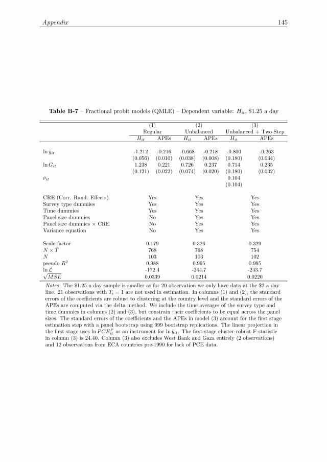
Appendix 145
Table B-7 – Fractional probit models (QMLE) – Dependent variable: Hit, $1.25 a day
(1) (2) (3)Regular Unbalanced Unbalanced + Two-Step
Hit APEs Hit APEs Hit APEs
ln yit -1.212 -0.216 -0.668 -0.218 -0.800 -0.263(0.056) (0.010) (0.038) (0.008) (0.180) (0.034)
lnGit 1.238 0.221 0.726 0.237 0.714 0.235(0.121) (0.022) (0.074) (0.020) (0.180) (0.032)
νit 0.104(0.104)
CRE (Corr. Rand. Effects) Yes Yes YesSurvey type dummies Yes Yes YesTime dummies Yes Yes YesPanel size dummies No Yes YesPanel size dummies × CRE No Yes YesVariance equation No Yes Yes
Scale factor 0.179 0.326 0.329N × T 768 768 754N 103 103 102pseudo R2 0.988 0.995 0.995lnL -172.4 -244.7 -243.7√MSE 0.0339 0.0214 0.0220
Notes: The $1.25 a day sample is smaller as for 20 observation we only have data at the $2 a dayline. 21 observations with Ti = 1 are not used in estimation. In columns (1) and (2), the standarderrors of the coefficients are robust to clustering at the country level and the standard errors of theAPEs are computed via the delta method. We include the time averages of the survey type andtime dummies in columns (2) and (3), but constrain their coefficients to be equal across the panelsizes. The standard errors of the coefficients and the APEs in model (3) account for the first stageestimation step with a panel bootstrap using 999 bootstrap replications. The linear projection inthe first stage uses lnPCEPit as an instrument for ln yit. The first-stage cluster-robust F-statisticin column (3) is 24.40. Column (3) also excludes West Bank and Gaza entirely (2 observations)and 12 observations from ECA countries pre-1990 for lack of PCE data.

146 Appendix
Table B-8 – Poverty projections (Hit × 100), preferred specification, $1.25 a day
2010 2010 2015 2020 2025 2030Official Estimate Estimate Estimate Estimate Estimate
East Asia & Pacific 12.48 9.63 5.09 2.76 1.60 1.00Europe & Central Asia 0.66 0.74 0.44 0.27 0.16 0.10Latin America & the Caribbean 5.53 5.59 4.84 4.22 3.70 3.26Middle East & North Africa 2.41 3.43 2.48 1.82 1.37 1.06South Asia 31.03 33.81 23.89 16.09 10.53 6.89Sub-Saharan Africa 48.47 46.87 42.95 39.84 37.20 34.86
World Total 20.63 20.44 15.82 12.66 10.58 9.27
Notes: Regional aggregates are based on the World Bank classification of low and middle incomecountries in 1990. High income countries in 1990 are assumed to have no poor. The projections arefor 123 countries. West Bank and Gaza is excluded as we lack both PCE and population data.
Figure B-5 – Predicted regional poverty, $1.25 a day, 2010 to 2030
0.0
0.1
0.2
0.3
0.4
2010 2015 2020 2025 2030
Poverty
Headcount(H
it)
EAP
ECA
LAC
MNA
SAS
SSA
1155.3
948.4
800.5
701.9
641.3
0
300
600
900
1200
2010 2015 2020 2025 2030
Poor
Pop
ulation
(Hit×
pop
it)
EAP
ECA
LAC
MNA
SAS
SSA

Chapter 6
Poor trends
The pace of poverty reduction after the Millennium
Development Agenda∗
Abstract
This chapter reviews the origins of the dollar-a-day poverty line, discusseshistorical poverty and inequality trends, and forecasts poverty rates until 2030using a new fractional response approach. Three findings stand out. First,global poverty reduction since 1981 has been rapid but regional trends areheterogeneous. Second, the pace of poverty reduction at $1.25 a day willslow down. Our optimistic scenarios suggest a poverty rate of 8-9% in 2030,far short of the World Bank’s new 3% target. Third, rapid progress can bemaintained at $2 a day, with an additional one billion people crossing thatline by 2030.
Keywords: poverty, inequality, consumption growth
JEL Classification: I32, O10, O15
∗This chapter is based on Bluhm, R., de Crombrugghe, D., and A. Szirmai. 2013. Poor trends- The pace of poverty reduction after the Millennium Development Agenda, MERIT Working Papers006, United Nations University - Maastricht Economic and Social Research Institute on Innovation andTechnology (MERIT).
147

148 Chapter 6. Poor trends
1 Introduction
“We are at an auspicious moment in history, when the successes of past decades and anincreasingly favorable economic outlook combine to give developing countries a chance, forthe first time ever, to end extreme poverty within a generation” (Jim Yong Kim, WorldBank President, speaking at Georgetown University, April 3, 2013)
Only 13 years after the Millennium Summit in September 2000 at which world leadersagreed on halving the 1990 global poverty rate at $1.25 a day by 2015, the end ofextreme poverty seems to be in sight. Recent estimates suggest that the first MillenniumDevelopment Goal (MDG) was already reached in 2010 and about 700 million peoplewere lifted out of poverty. In 2013, the World Bank declared a new organizational goal ofending extreme poverty by 2030, that is, reducing the $1.25 a day poverty rate to 3% by2030. The last two decades clearly ushered in unprecedented success, but is 2030 reallylikely to mark the end of extreme poverty? Our main contribution is to demonstrate thatthis is unlikely.
In this chapter, we review the origins of the ‘dollar-a-day’ poverty line, discuss progressover the last three decades, and forecast $1.25 and $2 a day poverty rates until 2030. Itis well-known that regional trends in poverty alleviation are very heterogeneous. In spiteof rising inequality, rapid growth in China was the driving force behind global progressover the last two decades and accounts for more than three quarters of the reduction inthe number of people living below $1.25 a day. However, most of the poverty reductionpotential coming from China is now exhausted. Poverty reduction in the developing worldoutside China has been considerably slower, although economic growth has acceleratedsignificantly since 2000. In 2010, three-fourths of the extremely poor lived in Sub-SaharanAfrica and South Asia, as opposed to approximately 40% in 1981. This changing regionalcomposition of world poverty has important ramifications for future trends in povertyreduction. The number of inhabitants of historically fast growing countries make up lessand less of the global poor.
Building on a new method for estimating poverty elasticities and predicting povertyheadcount ratios developed in Chapter 5, we show that the pace of poverty reduction at$1.25 a day is likely to slow down significantly after 2015. Extreme poverty barely fallsbelow 8% in the most optimistic scenario. Ravallion (2013) first suggested the 3% targetrelying on the assumption that consumption in developing countries would continue togrow at the average post-2000 trend, or 4.5% per year. We find this ‘equal-growth’assumption too optimistic. Poverty tends to be higher in countries with rapid populationgrowth and lower than average consumption growth. None of our scenarios predicts apoverty rate near 3% once country-specific trends from 2000 to 2010 are used. However,the $2 a day poverty rate may fall below 20% in 2030, while a slowdown happens onlylate during the forecast period or not at all. A distinct advantage of our approach is thatit is computationally inexpensive. Hence, it can easily be used for benchmarking progressas new data become available.
The chapter is structured as follows. Section 2 discusses some of the controversiessurrounding the setting and updating of international poverty lines. Section 3 is a data-driven review of global poverty and inequality trends with a particular focus on China,India, Brazil and Nigeria. Section 4 presents projections of global and regional povertyrates until 2030 at the $1.25 and $2 a day poverty lines using different growth andinequality scenarios. Section 5 concludes and offers some policy recommendations.

Drawing the line: international poverty lines 149
2 Drawing the line: international poverty lines
The dollar-a-day poverty line was first defined in a background paper to the 1990 WorldDevelopment Report (in 1985 PPPs), then updated to $1.08 (in 1993 PPPs) in 2000, andagain updated to $1.25 (in 2005 PPPs) in 2008. While the first update went by almostunnoticed, the most recent change has sparked a controversy. Redefining extreme povertyas living below $1.25 a day raised the global poverty headcount by about 10 percentagepoints and reclassified approximately 450 million people as extremely poor (Chen andRavallion, 2010). In this section, we briefly review the origins of the $1 a day measureand discuss shortcomings of the current updating procedure.
The problem of setting a global poverty line is far from trivial. Even if we coulduse a ‘basic needs’ or calorie-intake approach to devise a minimum consumption bundlefor the entire world, it is inherently difficult to apply any such bundle in internationalcomparisons. Subsistence needs, relative prices, and purchasing power vary acrosscountries and over time. Faced with these problems, Ravallion, Datt, and van de Walle(1991, henceforth RDV) suggested an original solution. Since many national povertylines are set using a basic needs or calorie-intake method, there should be a universallower bound among the absolute poverty lines which may be recovered from the data.Converting 33 national poverty lines and the corresponding consumption levels from the1970s and 1980s into international dollars, RDV showed that a poverty line of about $31per month ($1.02 a day, in 1985 prices) was shared by the six poorest countries in theirsample, while those of two other countries came close. They argued that a rounded-offpoverty line of $1 a day was a sensible threshold for measuring global poverty, since anyone poverty line is likely to be estimated with error and the non-food allowance includedin the subsistence basket varies across countries. RDV also estimated a lower line of $23per month (about 76 cents a day) for the poorest country in their sample. This lower linewas close to India’s poverty line at the time and became widely used as the internationalpoverty line during the 1970s and 1980s (e.g. Ahluwalia, Carter, and Chenery, 1979).
Setting the poverty line in international prices has the advantage that domesticinflation is typically taken into account when average incomes or expenditures fromsurveys are converted into (base year) international dollars, so that the line itself doesnot have to be explicitly updated annually. However, purchasing power parities (PPPs)change over time as countries grow richer (due to the Balassa-Samuelson effect). Inaddition, the quality of PPP estimates has been improving substantially with eachround of the International Comparison Program (ICP), so that updates are neededapproximately every decade. When the 1993 ICP data became available, Chen andRavallion (2001) revised the $1 a day line to $1.08 in 1993 prices. Using the same dataas in the original study, they found that $1.08 a day was the median poverty line of theten poorest countries. However, when the 2005 ICP was completed, instead of convertingthe old poverty line to 2005 prices, new data were collected and the poverty line wasredrawn. Ravallion, Chen, and Sangraula (2009, henceforth RCS) compiled a data setof 74 national poverty lines to update the original analysis. They found that nationalpoverty lines do not rise with per capita consumption until a certain turning point (about$60 per month) but increase strongly thereafter (left panel, Figure 1). RCS set the globalline as the average poverty line of the 15 countries below this threshold, or $1.25 a dayin 2005 prices.
Deaton (2010), as well as Deaton and Dupriez (2011), take issue with this approach.They argue that updating the international poverty line based on new data leads to

150 Chapter 6. Poor trends
“graduation effects” when countries move out of the reference group. They illustrate theircase using India and Guinea Bissau as examples. India was part of the initial referencegroup in RDV, and both countries appear in RCS’s more recent reference group. Indiahas a relatively low poverty line ($0.90 a day in 2005 prices) and a population of morethan a billion people, whereas Guinea Bissau has a higher poverty line ($1.51 a day in2005 prices) and is home to less than 1.5 million people. As average consumption inIndia grew considerably until 2000, it crossed the $60 threshold and is no longer partof the reference group. Even though the average Indian has become richer, both theinternational poverty line and the global poverty headcount increased as a result of Indiadropping out of the average. With Guinea Bissau the case is reversed. Its poverty lineis currently part of the average. A move out of the reference group would entail a fall inthe global poverty line and a reduction in global poverty that is many times greater thanthe population of Guinea Bissau. The left panel of Figure 1 illustrates this relationship.The bold horizontal line marks the $60 per month threshold (labeled RCS’09).
Figure 1 – Poverty lines and consumption levels around 2000
China
Guinea Bissau
India
RCS’09 DD’11
$1.25 a day
$2.00 a day
0100
200
300
Povert
y lin
e p
er
capita (
month
ly)
3 4 5 6 7Log per capita consumption (monthly)
(a) unweighted
China
Guinea Bissau
India
RCS’09 DD’11
$1.25 a day
$2.00 a day
0100
200
300
Povert
y lin
e p
er
capita (
month
ly)
3 4 5 6 7Log per capita consumption (monthly)
(b) population−weighted
Notes: Authors’ calculations using the data reported in Ravallion et al. (2009) and following theillustration of Deaton (2010). The non-linear trends are estimated using a (weighted) local linearsmoother with bandwidth 0.8.
A related issue is that the ICP data are primarily designed for comparing living standardsof entire populations, not just poor people. The typical consumption basket of the poor,and the associated price level, may be very different than the reference basket used forcomputing PPPs.
To address both the graduation issue and the PPP issue, Deaton and Dupriez (2011)propose using an alternative procedure. Linking consumption surveys to ICP data for the50 poorest countries, they simultaneously estimate the poverty line and PPPs of thosenear the poverty line (PPPs for the poor, or P4s). This yields lower poverty lines inbetween $0.92 and $1.19 a day. However, the effect of the P4s on the global povertycounts – at similar poverty lines – is relatively small. The resulting estimates of globalpoverty are lower primarily due to the lower poverty lines and not due to differences inrelative prices.

Drawing the line: international poverty lines 151
To an extent, the Deaton-Dupriez criticism can be addressed within the RCS approachby (1) weighting the national poverty lines by population sizes, and (2) extending thereference group of “poorest” countries. The Deaton-Dupriez proposal, labeled DD’11below, is to select the 50 poorest countries to constitute a fixed reference group. Clearly,the threshold of 50 countries is arbitrary. A possible alternative is to replicate the RCSapproach but estimate the consumption gradient using population weights instead ofequal weights (right panel, Figure 1). This is the approach proposed here. Examiningthe plot to find the point where the slope of consumption begins to be positive, we visuallyidentify a threshold of about 5 log dollars or $148.41 per month (C∗), which is just under$5 a day. There are 39 countries below this line, suggesting an alternative reference groupconsisting of those 39 countries. A population-weighted average of the national povertylines for this group implies a global poverty line of $1.06 a day whereas the simple averageis $1.46 a day (both in 2005 prices).
Table 1 – Estimates of the international poverty line (Z∗)
Consumption International Poverty Lines (in 2005 PPPs)
Estimation Equally-weighted Population-weighted
Sample ln(C∗) C∗ Z Z∗ Q50(Z) Z Z∗ N
RCS’09 4.09 60.00 1.25 1.25 1.27 1.17 1.17 15Alternative 5.00 148.41 1.46 1.46 1.38 1.06 1.06 39DD’11 5.53 251.59 1.76 1.26 1.51 1.12 1.00 50Full sample 6.50 668.31 2.91 1.46 2.00 1.84 1.06 74
Notes: Authors’ calculations using the data reported in Ravallion et al. (2009). Z is the(unweighted or weighted) average poverty line. Q50(Z) is the (unweighted) median poverty line.The regression based columns estimate the average level of the poverty line before theconsumption gradient turns positive. Following Ravallion et al. (2009), we obtain Z∗ fromZi = Z∗Ii + (α+ βCi)× (1− Ii), where Zi is the national poverty line expressed in 2005 PPPs, Z∗
is the mean poverty line for the reference group, Ci is average per capita consumption in 2005PPPs, and Ii is one if Ci ≤ C∗ and zero otherwise; that is, it indicates whether the country is in thereference group. This method imposes that the slope is zero until a monthly consumption level C∗.
Table 1 provides alternative estimates of the international poverty line using differentapproaches, references groups and weights. We can fully reproduce the main findings ofRCS. The average poverty of the poorest 15 countries is $1.25 a day and the full samplemedian is $2 a day. Three other results stand out. First, all estimates are above or equalto $1 a day in 2005 prices. Second, population weights lead to universally lower estimatesof the poverty line. Third, the estimated poverty line is fairly sensitive to both the choiceof C∗ and the summary measure (mean, median, weighted or not). While this lendssome support to the notion that $1.25 is a relatively high upward revision, the choice ofmethod, cutoff and weights remains subjective. Moreover, updating the old $1.08 povertyline in 1993 prices to $1.25 in 2005 prices implies a (global) inflation rate of about 1.2%per year. Precisely this point leads Chen and Ravallion (2010) to argue that “as long asit is agreed that $1 in 1993 international prices is worth more than $1 at 2005 prices,the qualitative result that the new ICP round implies a higher global poverty count isrobust” (p. 1612). In the following section, we will consider the policy consequences ofusing both $1.25 a day and the full-sample median of $2 a day as absolute poverty lines(a common practice in the literature, e.g. see Chen and Ravallion, 2010).

152 Chapter 6. Poor trends
Counting the global poor involves several difficult methodological choices on top ofchoosing an international poverty line that can have large effects on the estimated povertyrates.1 The inherent difficulty of convincingly solving these issues led some to suggestthat the current approach should be abandoned (e.g Klasen, 2009; Reddy and Pogge,2010). One alternative is to set national poverty lines in local currencies using the samemethod in each country. While this approach tries to sidestep the issue of purchasingpower parity comparisons altogether, it would certainly raise new problems. Alas, aconsiderable degree of indeterminacy regarding the level of extreme poverty in the worldseems unavoidable (but more is known about rates of change which we discuss in thenext section).
3 Taking stock: poverty reduction over the past
three decades
While the global Millennium Development Goal (MGD) of halving the $1.25 a day povertyrate in 1990 by 2015 was reached in 2010 (Chen and Ravallion, 2013), progress has beenvery uneven across regions. Most poverty reduction over the last three decades occurredin East Asia and, to a lesser extent, in South Asia. Poverty in Sub-Saharan Africa, onthe contrary, has hardly budged and the continent as a whole will – most probably – failto meet the first MDG by 2015.
Figure 2 shows population-weighted time trends estimated for each region using thenationally representative household surveys available in the World Bank’s PovcalNetdatabase (using consumption-based data where available). A pooled weighted leastsquares regression of the poverty headcount ratio on time for all developing countriesreveals that the poverty headcount at the $1.25 a day line fell by an average 1.5 percentagepoints per year (cluster t2 = -4.11). There is substantial regional heterogeneity. Onaverage, poverty fell by 2.21 percentage points annually in East Asia and Pacific (clustert = -10.08), by about 1 percentage point in South Asia (cluster t = -4.82), but onlyby 0.02 percentage points in Sub-Saharan Africa (cluster t = -0.05). In the other threedeveloping regions progress has been slow but steady. In Europe and Central Asia, LatinAmerica and Caribbean, and Middle East and North Africa the estimated slopes imply anexpected annual fall of 0.05 (cluster t = -1.91), 0.30 (cluster t = -5.76) and 0.14 (clustert = -2.40) percentage points, respectively. Using an alternative $2 a day poverty line, themagnitudes and differences in speeds across regions remain broadly similar.3
An important question is whether consumption growth or redistribution is drivingthe decline in poverty. Estimating the historical contributions of growth and changes indistribution during the 1980s and 1990s, Kraay (2006) found that most poverty reductionwas due to income or consumption growth. Our analysis broadly corroborates this finding
1For example, it is not clear that the ICP 2005 provides an adequate picture of the consumptionpatterns in the 1980s or 1990s. Another issue is the use of survey means versus national accounts means.The use of national accounts typically leads to much lower poverty estimates. See Sala-i-Martin (2006),Pinkovskiy and Sala-i-Martin (2009), and, in particular, Dhongde and Minoiu (2013) for a comparisonof different methods.
2Throughout the text, “cluster t” denotes a cluster-robust t-statistic, with clusters defined bycountries.
3East Asia and Pacific (slope = -2.31, cluster t= -7.33), Europe and Central Asia (slope=-0.26,cluster t=-2.33), Latin America and Caribbean (slope=-.55, cluster t = -5.74), South Asia (slope =-0.72, cluster t= -4.92), and Sub-Saharan Africa (slope = -0.02, cluster t= -0.07).

Taking stock: poverty reduction over the past three decades 153
Figure 2 – Population-weighted poverty trends by region, 1981 to 2010, $1.25 a day
05
01
00
05
01
00
1980 1990 2000 2010 1980 1990 2000 2010 1980 1990 2000 2010
East Asia and Pacific Europe and Central Asia Latin America and Caribbean
Middle East and North Africa South Asia Sub−Saharan Africa
Po
ve
rty H
ea
dco
un
t a
t $
1.2
5 a
da
y
Notes: Authors’ calculations based on surveys from PovcalNet.
(although we do not explicitly estimate contributions). The population-weighted growthrate of the survey means from 1981 to 2010 across all countries is a very robust 4% peryear (cluster t = 3.03). Over the same period, within-country inequality, as measure bythe Gini coefficient, actually increased slightly by about 0.7% per year (cluster t = 1.64).This implies that, on average, changes in distribution may have in fact moderately slowedthe pace of poverty reduction. Poverty reduction over the last three decades has mostlybeen due to income and consumption growth. However, both the high average growthrate in the survey means and the apparent rise in within-country inequality are drivenby China. Excluding China, the survey means grew about 1.8% per year (cluster t =2.45) and inequality barely moved (increased 0.047% per year, cluster t = 0.13). In otherwords, poverty reduction in the developing world outside China has been steady but slowand has (on average) not been helped by improvements in distribution.4
These findings are also in line with estimates of poverty at the $1.25 a day povertyline reported by the World Bank (see Appendix Table A-1). Chen and Ravallion’s (2010)estimates indicate rapid progress in China, little improvement in Sub-Saharan Africa,and moderate poverty reduction elsewhere. The poverty headcount ratio in Sub-SaharanAfrica only fell by about three percentage points over the entire period from 1981 to2010, and actually exceeded its 1981 value for most of the period. Combining thesetrends with population growth rates reveals the dire absence of a robust positive trendin terms of the number of global poor outside of East Asia. While China has lifted anastonishing 680 million people out of poverty between 1981 and 2010, the rest of theworld has only about 50 million fewer extremely poor people in 2010 than in 1981. This
4Excluding India in addition to China from the sample does not qualitatively alter this result.

154 Chapter 6. Poor trends
trend is due to persistently high poverty rates coupled with strong population growth inSub-Saharan Africa and India. This is most evident in Sub-Saharan Africa where thenumber of extremely poor has roughly doubled over three decades (in spite of the slightdecrease in the headcount ratio). The rise of China from a poor to a middle incomecountry also implies that the relative composition of world poverty is changing rapidly.In 1981 about 40% of the world’s extremely poor lived in Sub-Saharan Africa and SouthAsia, by 2010 their share has risen to 75%.
A very intuitive approach to illustrating past progress (or lack thereof) is toapproximate the shape of the income or expenditure distribution at various points intime and examine how the features of the distribution (esp. quantiles) shift over time.Figures 3 and 4 plot the lower tail (up to $400) of the monthly income or expendituredistribution for the most populous country of the four poorest regions – East Asia, SouthAsia, Latin America, and Sub-Saharan Africa – in 1985, 1990, 2000 and 2010. Thevertical lines are the $1.25 and $2 a day poverty lines in terms of monthly consumption.After lining up the survey data in time, we estimate the different density functions usinga log-normal approximation.5 While the assumption of log-normality has its weaknesses6,it usually provides a useful first estimate of the shape of the income distribution. A keyadvantage is that it only requires knowledge of the mean and Gini coefficient.
We can illustrate a few essential concepts with these graphs. The area under thecurve to the left of the poverty line gives the fraction of the population that is poor (thepoverty headcount ratio), while the spread of the distribution reflects inequality. The rawdifference between two such areas under the curve is the absolute change in the povertyheadcount ratio in percentage points and the relative difference gives the percent changein the poverty headcount ratio. The sensitivity of poverty reduction to changes in incomeor inequality is often measured in the form of elasticities or semi-elasticities. The incomeelasticity of poverty is the percent change in poverty for a one percent increase in incomes,and the income semi-elasticity of poverty is the percentage point difference in povertyfor a one percent increase in incomes. The inequality elasticity and semi-elasticity aredefined analogously. An attractive feature of the semi-elasticity is that it first increasesand then decreases again during the development process. It measures the pace of povertyreduction in terms of the percentage of the population lifted out of poverty. Hence, itis usually more informative for policy-makers and more useful than reporting relativechanges.7
Figure 3 visualizes the tremendous progress in reducing poverty rates in China overthe last three decades.8 As noted before, poverty in China at $1.25 a day fell rapidly
5We interpolate and extrapolate the data as follows. First, we project mean consumption forward andbackward using the corresponding growth rates of personal consumption expenditures from the nationalaccounts. Second, we linearly interpolate between the available Gini coefficients and extrapolate beyondthe first or last available measure by keeping inequality constant. The same data set (with all countriesfrom PovcalNet) is later used for computing the inequality indices in the developing world.
6Log-normality typically works better with consumption surveys than with income surveys (Lopezand Serven, 2006), tends to underestimate the level of poverty (Dhongde and Minoiu, 2013), andoverstates the pace of poverty reduction (Bresson, 2009).
7In relatively rich countries with low percentages of people below the poverty line, elasticities can bevery misleading. Small reductions in the poverty headcount rate can manifest themselves as very highelasticities. For a more detailed discussion of the properties of elasticities and semi-elasticities of povertysee Bourguignon (2003), Klasen and Misselhorn (2008), and Chapter 5.
8The implied poverty rates for China correspond well with the official World Bank estimates. At the$1.25 a day poverty line, our estimates imply a poverty rate of 60.56% in 1985, 56.92% in 1990, 31.97%in 2000 and 9.75% in 2010.

Taking stock: poverty reduction over the past three decades 155
Figure 3 – Estimates of the expenditure distribution: China and India, 1985–20100
.005
.01
.015
.02
Density (
Share
of P
opula
tion)
0 38 60.83 100 200 300 400Income/ Expenditure in PPP$ per month
1985
1990
2000
2010
China
0.0
05
.01
.015
Density (
Share
of P
opula
tion)
0 38 60.83 100 200 300 400Income/ Expenditure in PPP$ per month
1985
1990
2000
2010
India
Notes: Author’s calculations. China’s expenditure distribution is estimated based on a weightedmean and a rural-urban ln-mixture for the Gini coefficient. China’s surveys in PovcalNet areconsumption-based after 1987 and income-based before.
over the entire period. The biggest gains occurred early on, between 1985 and 2000,when the peak of the distribution was close to the $1.25 and $2 poverty lines. By 2010,the peak of the distribution has moved considerably to the right of both poverty linesand the overall spread has widened. A great many Chinese are now considered part ofa developing country ‘middle class’ (if defined between $2 and $13 per day).9 However,this also implies that the poverty reduction potential from China is largely exhausted.The income semi-elasticity of the poverty headcount is far beyond its peak and steadilyapproaching zero. In addition, inequality has increased remarkably over the same period.In 1985, the Gini coefficient was 0.28 and by 2010 it has risen to 0.44.
In India, on the contrary, there remains much greater potential for poverty reductionin the medium-term future. While the mode of the income distribution was near the$1.25 line around 1985 and 1990, the peak of the distribution in 2000 and 2010 is locatedbetween the two poverty lines. The process of “bunching up” in front of $2 a day observedby Chen and Ravallion (2010) implies that, in the medium-term future, the pace ofpoverty reduction in India (defined as the absolute change in the headcount) will beparticularly fast at the $2 a day line and continue at a fast but decelerating pace at the$1.25 line. Put differently, India’s income semi-elasticity around 2010 is very high anda moderate rate of growth will immediately have a large (but decreasing) effect on thepoverty headcount ratio at both thresholds.
Figure 4 illustrates two very different cases. The left panel shows that from 1985 to1990 poverty reduction in Brazil was very slow, with some progress at the $2 a day linebut a nearly unchanged poverty rate at the $1.25 line. Yet, on average, Brazilians werealready considerably better-off in the 1990s than their Chinese or Indian counterparts in
9Ravallion (2010) defines the size of the ‘middle class’ by developing country standards as theproportion of the population living on at least $2 per day but less than $13 per day, where the upperbound is the poverty line in the United States. Naturally, this is one of many possible definitions.

156 Chapter 6. Poor trends
Figure 4 – Estimates of the expenditure distribution: Brazil and Nigeria, 1985– 20100
.0005
.001
.0015
.002
Density (
Share
of P
opula
tion)
0 38 60.83 100 200 300 400Income/ Expenditure in PPP$ per month
1985
1990
2000
2010
Brazil
0.0
05
.01
.015
Density (
Share
of P
opula
tion)
0 38 60.83 100 200 300 400Income/ Expenditure in PPP$ per month
1985
1990
2000
2010
Nigeria
Notes: Authors’ calculations. Brazil’s distribution is based on incomes instead of expenditures.The 2010 data for Nigeria was revised in late 2014 (not incorporated here).
2010. After 1990, the pace of poverty reduction accelerates and by 2010 only 4.92% of thepopulation were below the $1.25 a day poverty line.10 Lifting the remaining people outof poverty will require sustained economic growth, as both the income and distributionsemi-elasticities of poverty in Latin America as a whole are rather low (see Chapter 5).With a Gini of 0.56 in 1985 income inequality was initially very high in Brazil, peaked at0.61 in 2000 and then fell again to 0.55 by 2010, thus positively contributing to povertyreduction after 2000. The right panel illustrates that poverty in Nigeria was considerablyhigher in 2000 or 2010 than in 1985. Nigeria’s plight is characteristic for most of Sub-Saharan Africa in the 1980s and 1990s, as real consumption on the subcontinent wasdeclining at a pace of about 0.82% per year. Only after 2000 did expenditures recoverand the poverty headcount ratio began to decline. Yet even by 2010, the peak of theexpenditure distribution is still noticeably to the left of the poverty line and the impliedpoverty rate at $1.25 a day is 65.96%.11 In addition, inequality in Nigeria increases overthe observed period, starting from a Gini of 0.39 in 1985 to 0.49 in 2010.
Taken together, these four distributions exemplify the changing composition of globalpoverty and broadly represent the trends in their respective regions. Over the lastthree decades, most poverty reduction occurred in East Asia where consumption growthwas fastest, some poverty reduction occurred in India where real consumption growthwas steady, and little poverty reduction occurred in Sub-Saharan Africa where realconsumption growth was slow and volatile. This suggests that without significantly fastergrowth in Sub-Saharan Africa than in the past, possibly coupled with improvements in theincome or expenditure distribution, the global pace of poverty reduction will inevitablyslow down in the near future.
Another essential aspect of poverty analysis is studying the evolution of inequality.In this part, we focus only on inequality among citizens of developing countries, as
10The World Bank estimated a poverty rate of 5.38% at $1.25 a day for Brazil in 2010.11The World Bank estimated a poverty rate of 67.98% at $1.25 a day for Nigeria in 2010.

Taking stock: poverty reduction over the past three decades 157
our interest is the changing relative position of people in the developing world ratherthan their position vis-a-vis rich countries. Interestingly, many of the global trends arealso evident even when we restrict our attention to this truncated distribution. Wecompute three measures of inequality by applying Young’s (2011) mixture of log-normaldistributions approach to the PovcalNet data. ‘Overall inequality’ is the Gini coefficientfor citizens of developing countries regardless of their country of residency. ‘Withininequality’ is a population-weighted summary measure of inequality within each country.Last, ‘between inequality’ is the population-weighted Gini coefficient of average incomesamong all developing countries. In other words, the first measure encompasses boththe within-country and between-country components that make up overall inequality inthe developing world. Naturally, global inequality – including the citizens of developedcountries – is typically estimated to be considerably higher. Recent estimates of the globalGini suggest that it is around 0.65-0.70, and may be even higher if underreporting of top-incomes is taken into account (e.g. see Pinkovskiy and Sala-i-Martin, 2009; Milanovic,2012; Chotikapanich, Griffiths, Rao, and Valencia, 2012; Lakner and Milanovic, 2013).
Table 2 – Inequality in the developing world, 1980–2010
Gini coefficient
Year Overall Within BetweenMean
ConsumptionPopulation N
1980 0.596 0.356 0.486 73.29 2907.8 831985 0.555 0.353 0.421 79.05 3223.2 861990 0.578 0.367 0.449 95.98 4049.3 1041995 0.559 0.385 0.411 98.41 4555.2 1142000 0.537 0.395 0.374 102.45 4931.4 1212005 0.535 0.399 0.372 120.34 5285.6 1232010 0.554 0.404 0.399 150.72 5625.1 123
∆ 1980-2010 (in %) -7.19 13.63 -17.82 – – –∆ 1990-2010 (in %) -4.17 10.10 -11.08 – – –∆ 2000-2010 (in %) 3.07 2.20 6.64 – – –
Notes: Authors’ calculations. The sample size varies over the years. A total of 124 countries arerecorded in PovcalNet but we lack PCE data for West Bank and Gaza. The results are verysimilar if we constrain the developing world to consist of the 104 countries from which we have(interpolated) data from 1990 onwards. Due to the lower coverage, the results for the 1980s shouldbe interpreted with caution. For details on the ln-mixture calculations refer to Young (2011).
Table 2 reveals some interesting trends. Overall inequality in the developing world hasbeen falling between 1990 and 2005, but it exhibits an increase in 2010. At the sametime, within-country inequality has been rising steadily since the mid-1980s. Between-country inequality fell over most of the period but also shows a slight increase between2005 and 2010. If we exclude China from the computations given that its weight isvery high, then these trends are considerably muted or even non-existent.12 Hence, two
12Overall inequality is estimated as 58.33 in 1990 and 58.36 in 2010, within-country inequality isestimated as 38.36 in 1990 and 39.12 in 2010, and between-country inequality is estimated as 45.04 in1990 and 45.44 in 2010. Removing India in addition to China has little effect on the trends in theinequality measures.

158 Chapter 6. Poor trends
developments drive the overall change. First, inequality of incomes within China has beenincreasing significantly and, second, its relative position among developing countries hasbeen changing rapidly. Rising mean incomes in China from the 1980s onwards initiallyimplied a reduction of between-country inequality as the average citizen in China wasmoving from the bottom towards the middle of the developing country ranks, but theynow put upward pressure on overall inequality as incomes in China continue to grow andthe distance from incomes in Sub-Saharan Africa increases.13
4 Going forward: poverty projections until 2030
As the expiration date of the MDGs is approaching quickly, new goals will have to beselected. Picking from among a wide range of possible benchmarks invariably involvesformulating expectations towards a fundamentally uncertain future. Thus, it becomesimportant to ask: what can the current data and methods tell us about the prospectsfor poverty alleviation over the next two decades? The list of policy-relevant questions islong. What level of poverty do we expect to prevail in 2030? Will it be feasible to trulyeradicate extreme poverty by 2030? Or, how quickly do we expect poverty rates underthe $2 a day poverty line to decrease? Here, we provide both a glimpse into several likelyfutures and some potential answers to these questions.
This section draws heavily on Chapter 5, where we develop a ‘fractional responseapproach’ for estimating income and inequality (semi-) elasticities of poverty. Amongother things, we that this new method can be used to easily forecast global poverty ratesusing only two variables (the survey mean and the Gini coefficient). A key advantage ofthis approach over, say, linear trend extrapolations, is that it builds in the non-linearityof the poverty-income-inequality relationship. Neither the income or inequality elasticitynor the income or inequality semi-elasticity is assumed to be constant. The methodaccounts for the fact that income growth will have an increasing effect in very poorcountries, where the mass of the distribution is to the left of the poverty line, and lessand less of an effect in rich countries, where the mass of the distribution is far to theright of the poverty line.14 Similarly, the effect of changes in distribution will indirectlydepend on the prevailing levels of both income and inequality.
We are of course not the first to present poverty projections over the next two decades.Ravallion (2013), for example, outlines an aspirational scenario where an additional billionpeople are lifted out of extreme poverty by 2025-2030. Karver, Kenny, and Sumner (2012)discuss the future of the MDGs more generally and simulate poverty rates at the $1.25and $2 a day poverty lines for 2030.15 Yet there are some important conceptual and
13This trend is corroborated by the literature on global inequality. According to Lakner and Milanovic(2013), average incomes in Sub-Saharan Africa were $742 in 1988 and only $762 in 2008 (in 2005 PPPs),while Chinese incomes increased by 228.9% and no longer make up a large part of the lower tail of theglobal income distribution. They also show that inequality within China has risen between 1988 and2008.
14The inability to account for countries that have relatively high incomes and zero poverty at somepoint in time (typically the beginning or end of a spell) is a key weakness of studies investigating povertyelasticities.
15Karver et al. (2012) allow for country-specific growth rates but use older data (their PovcalNetreference year is 2008) and disregard the difference between GDP per capita growth and growth of thesurvey mean. This leads them to overestimate the speed of poverty reduction relative to our forecasts.A recent study by Chandy, Ledlie, and Penciakova (2013) echoes some of our results. They use GDP percapita rather than consumption expenditure data for most of the period, but apply a conversion factor,

Going forward: poverty projections until 2030 159
methodological differences between our approach and these studies. First, the assumptionthat the developing world will continue growing at the accelerated 2000 to 2010 pacefor another twenty years (our optimistic scenario) is questionable. There is a well-known instability of growth rates across decades that should not be ignored (Easterlyet al., 1993), especially since the high average growth rates in the developing world weredriven by rapid growth in China. A more conservative assumption is that countrieswill grow at rates much closer to their individual long-run growth path. Second, thechanging composition of the countries contributing to global poverty matters a lot forthe expected speed of global poverty reduction. Unless there is a persistent accelerationof consumption growth in Sub-Saharan Africa on top of the post-2000 growth rates andsustained consumption growth in India, we can show that the pace of poverty reduction atthe $1.25 line is likely to experience a pronounced slowdown in all of our forecast scenarios(defined below). Third, pro-poor growth can potentially make a sizable difference in theexpected poverty rates, while a rise in within-country inequality will hasten the arrivalof the slowdown. Fourth, our method approximates the ‘official’ PovcalNet results at afraction of the computational cost, so that a variety of scenarios can be easily estimated(and frequently updated with the arrival of new data).
We define three different constant growth scenarios on the basis of the historicalpersonal consumption expenditure (PCE) growth rates from the national accounts.16 An‘optimistic’ scenario uses the average PCE growth rate of each country from 2000-2010,during which period growth rates were significantly higher than before 2000. A ‘moderate’growth scenario uses the average PCE growth rate of each country from 1980 to 2010– the long run average over the entire data set. Finally, a ‘pessimistic’ growth scenariouses the 1980 to 2000 average PCE growth rates. The latter scenario assumes that meanconsumption in Sub-Saharan Africa is shrinking at a rate of about 0.82% per year.17
Table A-2 in the Appendix reports the population-weighted average regional growth ratesover several different periods to illustrate the implied regional income dynamics.
For each growth scenario, we also simulate three different inequality patterns. ‘Pro-poor growth’ implies an annual decline in the Gini coefficient of approximately -0.5%,‘distribution-neutral growth’ keeps inequality constant at the level prevailing in 2010,and ‘pro-rich growth’ implies an increase in the Gini coefficient of approximately 0.5%per year.18 As an illustration, if a country’s Gini coefficient is 0.40 in 2010 and we applythe pro-poor pattern, then by 2030 we project a Gini coefficient of about 0.36. If weapply the pro-rich pattern, then the Gini coefficient is about 0.44 in 2030. Changes ofthis magnitude are in line with the population-weighted regional trends obtained fromthe surveys.
We forecast the poverty rates until 2030 as follows. First, we estimate the modeloutlined in Chapter 5 for the $1.25 a day poverty line using all nationally-representativesurveys recorded in PovcalNet over the period from 1981 to 2010. Next, after lining upall surveys in 2010, we apply each of the nine growth and distribution scenarios to projectthe income and inequality data forward to 2030, country by country.19 Then, we predict
and report lower poverty estimates.16The term ‘national accounts’ refers to data from the World Development Indicators or the Penn
World Table 7.1, whichever has more data over the 30 year horizon.17Owing to the post-communist transition, consumption and incomes in Europe and Central Asia
were shrinking over the same period. However, given the small number of poor in 2010, the influence ofthat region on the global poverty headcount in 2030 is minimal.
18All reported growth rates (in percent) are computed as log differences if not otherwise noted.19To line up all surveys in 2010, we use the actually observed PCE growth rates from the national

160 Chapter 6. Poor trends
the poverty headcount ratios in five-year intervals over the period 2015 to 2030, countryby country. Finally, we calculate population-weighted regional poverty rates and applythese to the projected total population in each region. For consistency with PovcalNet,the population projections are also taken from the World Bank and the ‘developing world’is defined as in 1990 – the countries targeted by the MDGs – no matter how high weforecast the average level of consumption to be in 2030. Contrary to the World Bank’srecent redefinition of the denominator, we still focus on the percent of poor populationin the developing world and not the entire world.
Figure 5 – Actual and projected poverty headcount ratios at $1.25 a day, 1981–2030
Linear trend
Observed Data
Projections
01
02
03
04
05
0H
ea
dco
un
t ra
tio
at
$1
.25
a d
ay (
in %
)
1980 1990 2000 2010 2020 2030
Notes: Authors’ calculations based on Chapter 5 and survey data from PovcalNet. The solid blackline beyond 2010 refers to the moderate (distribution-neutral) growth scenario in Table 3, whilethe solid grey lines represent the distribution-neutral variants of the optimistic and pessimisticscenarios. The pro-poor and pro-rich variants are shown as grey dotted lines and are located aboveor below a solid line.
Figure 5 plots the historical evolution of the poverty headcount from 1981 to 2010, alinear trend fitted through the observed data and then extrapolated until 2030, and ourdifferent scenarios. The linear trend serves as a reference for the non-linear projections.Several points are noteworthy. First, only the linear extrapolation predicts a povertyrate in the vicinity of zero by 2030. Regressing the global poverty rate at $1.25 a dayon time one obtains a slope of about one percentage point per year (see also Ravallion,2013).20 As the global poverty rate was about 20.6% in 2010, the linear trend predicts
accounts to extrapolate the survey means from the latest available survey. In doing so, we keep inequalityconstant at the last observed Gini coefficient. In 2010, the average year when the last survey wasconducted is 2006.7, so about 3 years prior to 2010. More than 40% of the last surveys were conductedin 2009 or 2010.
20This differs from the 1.5 percentage points estimated in the previous section as the global povertyrate is measured by lining up and weighting all surveys at reference years (three year intervals from1981 onwards), whereas in the previous section we were using an unbalanced panel of unequally-spaced,

Going forward: poverty projections until 2030 161
that extreme poverty will have vanished by 2030. Second, all our projections show adecelerating rate of poverty reduction. Even in the most optimistic scenario, the paceof poverty reduction slows down. Most forecasts show a decelerating trend early on. Inthe optimistic scenario the slowdown only becomes noticeable by about 2020. Third, allscenarios but the optimistic pro-poor growth or optimistic distribution-neutral growthscenarios imply a poverty rate higher than 10% in 2030 at the $1.25 a day line. Theoptimistic pro-poor growth and distribution-neutral scenarios suggest a poverty rate in2030 of 7.9% and 9.1%, respectively. In a nutshell, 2030 is not likely to mark the end ofextreme poverty, even under very optimistic assumptions. Our projections suggest thatthe World Bank’s goal of 3% extreme poverty in 2030 is not likely to be reached.
Table 3 provides the corresponding regional and total poverty rates in 2030 includingthe expected number of poor in the various scenarios. Our moderate growth estimatesuggests a global poverty rate of 13.2% in 2030, implying about 950 million poor versus 1.2billion poor people in 2010. The pace of poverty reduction will have slowed significantlyboth in terms of relative changes and in terms of numbers of poor people. In this scenario,about 70% of the world’s poor live in Sub-Saharan Africa and about 23% in South Asiaby 2030. In contrast, the (distribution-neutral) optimistic result suggests a poverty rateof 9.11%, with about 655 million people remaining extremely poor. About 76% percentlive in Sub-Saharan Africa and about 17% in South Asia. The pessimistic case suggestsnext to no progress at all. Given an unchanged distribution, the poverty headcount ratiois estimated at 16.82% and the world is still home to 1.2 billion extremely poor people.Even if growth rates in Sub-Saharan Africa were to double relative to the post-2000 trend,the global poverty rate in 2030 is still projected to be 6.50% with pro-poor growth, 7.67%with distribution-neutral growth, and 8.81% with pro-rich growth.
All of these estimates imply that it will take considerably longer than 2030 to liftthe remaining 1.2 billion people out of poverty. The good news is that by 2030 extremepoverty in Europe and Central Asia, East Asia, Latin America, and Middle East andNorth Africa may virtually disappear (projected to be less than 5% in most forecasts).However, we predict a strong increase in the (relative) share of global poverty located inSub-Saharan Africa, which suggests that a non-trivial fraction of extreme poverty maybe concentrated in ‘fragile states’. Whether these countries will overcome civil strife,political instability and corruption will ultimately decide whether there is a lower boundat which extreme poverty will continue to exist.
Gradual changes in inequality raise or lower the overall headcount in between 1.2and 2.1 percentage points and account for about 100 million poor people more or less.Contrary to suggesting that inequality does not matter (we only assume slow changes),this finding hints at two crucial points. First, if the developing world as a whole is to trulymaintain the impressive record in poverty reduction of the last decades, then this requiresboth sustained high growth at the level experienced since 2000 and improvements indistribution. Second, any systematic worsening of within-country inequality, particularlyin large and largely poor countries like India or Nigeria, will reinforce the slowdown andthus more strongly decelerate the global rate of poverty reduction.
Readers may wonder why these results are so different from the projections reportedin Ravallion (2013). Our results differ mainly because Ravallion (2013) uses the averagegrowth rate of the developing world to project poverty in countries with very differenttrack records, while we use country-specific average growth rates. Otherwise there areonly minor differences in the data used and our method closely approximates results
population-weighted survey data with a wide yet somewhat selective coverage.

162 Chapter 6. Poor trends
Table
3–
Pro
ject
edp
over
tyh
ead
cou
nt
rati
os
and
poor
pop
ula
tion
at$1.
25a
day
in20
30,
by
regi
on
Ave
rage
PC
EG
row
th
Opti
mis
tic
(200
0-20
10)
Moder
ate
(198
0-20
10)
Pes
sim
isti
c(1
980-
2000
)
Cha
nge
inIn
equ
alit
y(G
ini)
pro
-poor
neu
tral
pro
-ric
hpro
-poor
neu
tral
pro
-ric
hpro
-poor
neu
tral
pro
-ric
h
Pan
el(a
)–
Hea
dcou
nt
at$1
.25
ada
yin
2030
(in
perc
ent)
Eas
tA
sia
and
Pac
ific
0.65
0.93
1.31
0.76
1.07
1.48
0.94
1.29
1.74
Euro
pe
and
Cen
tral
Asi
a0.
120.
160.
211.
211.
451.
715.
175.
746.
44L
atin
Am
eric
aan
dC
arib
bea
n2.
272.
743.
283.
464.
124.
914.
595.
466.
48M
iddle
Eas
tan
dN
orth
Afr
ica
0.48
0.66
0.91
1.54
2.07
2.75
3.72
4.77
6.05
Sou
thA
sia
4.19
5.54
7.24
8.48
10.8
913
.79
12.7
615
.99
19.7
7Sub-S
ahar
anA
fric
a32
.09
35.6
939
.37
43.6
247
.17
50.7
051
.75
55.1
258
.47
Tot
al7.
889.
1110
.49
11.6
313
.20
14.9
614
.96
16.8
218
.89
Pan
el(b
)–
Poo
rpo
pula
tion
at$1
.25
ada
yin
2030
(in
mil
lion
s)
Eas
tA
sia
and
Pac
ific
14.0
520
.23
28.5
616
.59
23.2
932
.22
20.4
428
.00
37.8
7E
uro
pe
and
Cen
tral
Asi
a0.
590.
760.
975.
726.
868.
1124
.47
27.1
630
.45
Lat
inA
mer
ica
and
Car
ibb
ean
16.1
519
.44
23.3
224
.61
29.3
034
.86
32.6
138
.77
46.0
5M
iddle
Eas
tan
dN
orth
Afr
ica
2.12
2.94
4.04
6.84
9.18
12.1
816
.47
21.1
526
.83
Sou
thA
sia
83.4
711
0.38
144.
3516
9.13
217.
0827
5.00
254.
4031
8.89
394.
16Sub-S
ahar
anA
fric
a44
9.54
499.
9755
1.61
611.
1566
0.85
710.
3272
5.03
772.
2681
9.22
Tot
al56
7.20
655.
3675
4.95
836.
3494
9.49
1076
.37
1076
.35
1209
.95
1359
.23
Note
s:A
uth
ors’
calc
ula
tion
s.P
op
ula
tion
pro
ject
ion
sare
from
the
Wor
ldB
an
k’s
Hea
lth
,N
utr
itio
nan
dP
op
ula
tion
Sta
tist
ics
data
base
.T
he
diff
eren
tsc
enar
ios
are
esti
mat
edu
sin
gth
efr
acti
on
al
resp
onse
app
roach
ou
tlin
edin
Ch
ap
ter
5an
dth
esu
rvey
data
rep
orte
din
the
Worl
dB
an
k’s
Povc
alN
etd
ata
base
.

Going forward: poverty projections until 2030 163
obtained using PovcalNet. Ravallion (2013) calculates that a PCE growth rate of 4.5%per year may bring the global poverty rate down to 3% by 2027. However, he makes the(in our view implausible) assumption that all developing countries will continue to growequally fast at this common rate of 4.5%. Likewise, the linear projection of the globalpoverty rate on time ignores all issues of aggregation and provides an overly optimisticpicture of the medium-term future.21 Yet composition matters, even if we incorporatethe optimistic assumption that the post-2000 trend will continue. The average hidesthat rapid growth is less likely in some countries than in others. As we have shown,this has direct consequences for when a slowdown will be observed and how strong thedeceleration will be. However, even if we assume a uniform growth rate for all developingcountries, a deceleration appears sooner or later within the next two decades (althoughit may actually be preceded by a brief acceleration if we assume growth rates in excessof 5% p.a.). It is comforting that, in line with Ravallion (2013), our method implies thatif consumption in the entire developing world grew at a distributional-neutral pace of7.6% per year, then extreme poverty would indeed virtually disappear by 2030 (fall to1.1%). The 3% target can be reached with a uniform distribution-neutral growth rate ofapproximately 5.5% per year.22
We repeat this exercise at the $2 a day poverty line. The results are reported inTable 4 and Figure A-1 in the Appendix. Interestingly, the linear projection is a muchbetter approximation of progress at the $2 poverty line than at the $1.25 poverty line.This is not due to a slower historical poverty reduction record: a regression of the globalpoverty rate at $2 a day on time also yields a slope of approximately one percentage pointper year. However, the composition of countries (or people) near the $2 a day povertyline in 2010 is more reminiscent of its $1.25 counterpart in the early 2000s. At the startof the decade in 2010, the total $2 poverty rate is 40.67% – roughly double the $1.25poverty rate. Fast growing East Asia and moderately fast growing South Asia still makeup more than half of global poverty, implying that progress in these two regions will havea large effect on the overall poverty headcount.
Our moderate growth scenario predicts that about 1.87 billion people (26%) liveon less than $2 a day in 2030 versus about 2.4 billion people in 2010. Considerablygreater gains are possible. Global poverty at the $2 line falls below 20% in the optimisticdistribution-neutral and pro-poor scenarios. If this occurs in 2030, then more than onebillion people will have left poverty at the $2 a day line – undeniably a remarkableachievement. In most scenarios we also observe a slowdown at the $2 a day line but thisslowdown tends to occur later and is less pronounced than at the lower threshold. In themost optimistic scenario, the rate of poverty reduction actually accelerates somewhat toabout 1.16 percentage points per year, while the moderate growth scenario gives a trendof 0.73 percentage points per year over the projection period.
Examining the regional distribution, we find that poverty in East Asia is likely tofall to around 5% by 2030, down from 29.7% in 2010. Nearly everyone in East Asiawill have entered the middle class (by developing country standards), but this forecastpartially hinges on fast growth in China. In fact, some observers suggest that there is
21We do not mean to imply that Ravallion (2013) is not aware of the aggregation issues. In fact, he usesPovcalNet precisely to confirm that his ‘optimistic scenario’ is possible once the intrinsic non-linearity ofthe poverty-income-inequality relationship is accounted for. Our point is rather that he envisions “thebest possible world” to be used as a benchmark for future progress while we also focus on other, morelikely, scenarios.
22Interestingly, a recent working paper by Yoshida et al. (2014), independently and using differentmethods, comes to very similar conclusions.
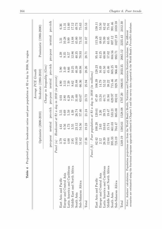
164 Chapter 6. Poor trends
Table
4–
Pro
ject
edp
over
tyh
ead
cou
nt
rati
osan
dp
oor
pop
ula
tion
at$2
ad
ayin
2030,
by
regi
on
Ave
rage
PC
EG
row
th
Opti
mis
tic
(200
0-20
10)
Moder
ate
(198
0-20
10)
Pes
sim
isti
c(1
980-
2000
)
Cha
nge
inIn
equ
alit
y(G
ini)
pro
-poor
neu
tral
pro
-ric
hpro
-poor
neu
tral
pro
-ric
hpro
-poor
neu
tral
pro
-ric
h
Pan
el(a
)–
Hea
dcou
nt
at$2
ada
yin
2030
(in
perc
ent)
Eas
tA
sia
and
Pac
ific
3.79
4.61
5.55
4.03
4.90
5.90
4.39
5.31
6.36
Euro
pe
and
Cen
tral
Asi
a0.
450.
560.
692.
803.
133.
499.
3510
.28
11.3
1L
atin
Am
eric
aan
dC
arib
bea
n4.
004.
735.
596.
297.
398.
668.
579.
9911
.60
Mid
dle
Eas
tan
dN
orth
Afr
ica
2.85
3.55
4.39
7.20
8.62
10.2
512
.86
14.8
817
.12
Sou
thA
sia
19.8
323
.12
26.7
431
.60
35.8
840
.39
40.3
545
.00
49.7
3Sub-S
ahar
anA
fric
a51
.62
54.5
657
.46
63.6
766
.36
68.9
870
.93
73.3
275
.63
Tot
al17
.36
19.2
321
.24
23.7
325
.94
28.2
628
.71
31.0
733
.53
Pan
el(b
)–
Poo
rpo
pula
tion
at$2
ada
yin
2030
(in
mil
lion
s)
Eas
tA
sia
and
Pac
ific
82.4
210
0.20
120.
6187
.49
106.
3912
8.23
95.4
411
5.26
138.
11E
uro
pe
and
Cen
tral
Asi
a2.
122.
633.
2613
.24
14.7
916
.49
44.2
548
.63
53.5
0L
atin
Am
eric
aan
dC
arib
bea
n28
.39
33.6
339
.73
44.7
152
.52
61.5
060
.90
70.9
982
.42
Mid
dle
Eas
tan
dN
orth
Afr
ica
12.6
415
.74
19.4
731
.94
38.2
245
.46
57.0
265
.95
75.9
1Sou
thA
sia
395.
3346
1.03
533.
2162
9.97
715.
4680
5.25
804.
5689
7.12
991.
46Sub-S
ahar
anA
fric
a72
3.19
764.
4780
5.00
892.
0192
9.76
966.
4899
3.71
1027
.19
1059
.59
Tot
al12
49.1
913
83.6
115
28.0
817
07.2
018
66.0
120
33.3
520
65.1
222
35.4
324
12.3
0
Note
s:A
uth
ors’
calc
ula
tion
s.P
op
ula
tion
pro
ject
ion
sare
from
the
Wor
ldB
an
k’s
Hea
lth
,N
utr
itio
nan
dP
op
ula
tion
Sta
tist
ics
data
base
.T
he
diff
eren
tsc
enar
ios
are
esti
mat
edu
sin
gth
efr
acti
on
al
resp
onse
app
roach
ou
tlin
edin
Ch
ap
ter
5an
dth
esu
rvey
data
rep
orte
din
the
Worl
dB
an
k’s
Povc
alN
etd
ata
base
.

Concluding remarks and policy recommendations 165
reason to believe that China runs a non-negligible risk of falling into a ‘middle-incometrap’ (Eichengreen, Park, and Shin, 2013) which might make it harder to achieve lessthan 10% poverty at $2 a day by 2030.23 Progress in South Asia is also likely to berapid. According to our moderate growth estimate the expected poverty rate is 35.9%in 2030, implying about 716 million poor, down from 66.7% and about 1.1 billion poorin 2010. In the optimistic pro-poor growth case, the headcount ratio falls by about onethird to less than 20% and the number of poor decreases to less than 400 million. As astark contrast, the $2 a day poverty rate in Sub-Saharan Africa is expected to remainvery high. Our moderate growth scenario predicts a poverty rate of about 66%, downfrom 69.9% in 2010, which at current population projections implies almost one billionpoor in Sub-Saharan Africa alone. Even in the optimistic distribution-neutral growthscenario, we project a poverty rate of about 55% and more than 750 million poor. Thisis underlined by the analysis in the preceding section where we suggest that the mass ofthe consumption distribution is far to the left of the $2 a day poverty line in 2010 formost of the subcontinent. Poverty alleviation in Sub-Saharan Africa remains the primarydevelopment challenge of the first half of the 21st century.
5 Concluding remarks and policy recommendations
The main contribution of this chapter is to forecast global poverty rates until 2030. To setthe stage, we first highlighted that there is a fundamental uncertainty about the preciselevels of extreme poverty. For the sake of comparison, we selected the standard povertylines of $1.25 and $2 a day (in 2005 PPPs). We then discussed a robust set of globalpoverty and inequality trends. The global MDG of halving the 1990 extreme poverty levelwas reached in 2010 but this apparent progress hides substantial regional heterogeneity.Most of the global success was driven by rapid growth in China. Inequality among thecitizens of developing countries and between developing countries was declining until2005, while average within-country inequality was rising steadily until 2010.
The changing composition of global poverty has profound implications for the medium-term future. After 2010, fast growing East Asia will contribute less and less to globalpoverty reduction, while the share of the global poor residing in Sub-Saharan Africa andSouth Asia will continue to rise. All of our projections show that the global rate ofpoverty reduction at $1.25 a day will slow down markedly between 2020 and 2025. Noneof our nine scenarios predicts a poverty rate near zero by 2030. This stands in starkcontrast to earlier studies and the ‘3% by 2030’ target recently announced by the WorldBank. The Bank’s target can only be reached if we make the unrealistic assumptionof equally rapid growth in all developing countries. Once country-specific growth ratesare used, even our most optimistic scenarios suggest a poverty rate of between 7.9% and10.5%, depending on the evolution of inequality. At $2 a day, the slowdown will occurmuch later and remarkable gains are possible if the post-2000 growth trends continue.An optimistic estimate suggests that the $2 a day poverty rate may fall below 20% by2030, implying one billion fewer poor people than in 2010.
We propose two new ‘twin targets’ on the basis of these findings. An aspirationalbut realistic benchmark for progress would be to “reduce the proportion of the populationliving below $1.25 to 8% by 2030 and reduce the proportion of the population living below
23However, our estimates suggest that this would require an exceptionally large slowdown. For povertyin East Asia to remain above 10% at $2 a day, growth needs to be less than half of the 2000-2010 trend.

166 Chapter 6. Poor trends
$2 a day to 18% by 2030.” Both of these targets are firmly anchored in our optimisticpro-poor growth scenarios. The $2 a day poverty line should receive more attention inthe future to better track continued progress in East Asia and, later on, South Asia.Partly for the same reason, China has recently raised its own national poverty line toabout $1.80 a day.
These targets can be reached in a variety of ways but not only through a continuationof the current path. They will require either an additional acceleration of growth in poorercountries, or improvements in distribution. Reversing the trend of rising within-countryinequalities would speed up the pace of poverty reduction and still ensure progress atmore moderate growth rates. The returns to redistribution are increasingly high in Eastand South Asia, and remain relatively large in Latin America. However, in some regionsgrowth takes precedent. Rapid poverty alleviation in Sub-Saharan Africa still requires asignificant and sustained acceleration in consumption growth.

Bibliography 167
Bibliography
Ahluwalia, M. S., N. G. Carter, and H. B. Chenery (1979). Growth and poverty in developing countries.Journal of Development Economics 6 (3), 299–341.
Bourguignon, F. (2003). The growth elasticity of poverty reduction: Explaining heterogeneity acrosscountries and time periods. In T. S. Eicher and S. J. Turnovsky (Eds.), Inequality and Growth:Theory and Policy Implications, pp. 3–26. Cambridge, MA: MIT Press.
Bresson, F. (2009). On the estimation of growth and inequality elasticities of poverty with grouped data.Review of Income and Wealth 55 (2), 266–302.
Chandy, L., N. Ledlie, and V. Penciakova (2013). The final countdown: Prospects for ending extremepoverty by 2030. Global Views Policy Paper 2013-04, Brookings Institution.
Chen, S. and M. Ravallion (2001). How did the world’s poorest fare in the 1990s? Review of Incomeand Wealth 47 (3), 283–300.
Chen, S. and M. Ravallion (2010). The developing world is poorer than we thought, but no less successfulin the fight against poverty. Quarterly Journal of Economics 125 (4), 1577–1625.
Chen, S. and M. Ravallion (2013). More relatively-poor people in a less absolutely-poor world. Reviewof Income and Wealth 59 (1), 1–28.
Chotikapanich, D., W. E. Griffiths, D. S. P. Rao, and V. Valencia (2012). Global income distributionsand inequality, 1993 and 2000: Incorporating country-level inequality modeled with beta distributions.Review of Economics and Statistics 94 (1), 52–73.
Deaton, A. (2010). Price indexes, inequality, and the measurement of world poverty. American EconomicReview 100 (1), 1–34.
Deaton, A. and O. Dupriez (2011). Purchasing power parity exchange rates for the global poor. AmericanEconomic Journal: Applied Economics 3 (2), 137–166.
Dhongde, S. and C. Minoiu (2013). Global poverty estimates: A sensitivity analysis. WorldDevelopment 44 (C), 1–13.
Easterly, W., M. Kremer, L. Pritchett, and L. H. Summers (1993). Good policy or good luck? Journalof Monetary Economics 32 (3), 459–483.
Eichengreen, B., D. Park, and K. Shin (2013, January). Growth slowdowns redux: New evidence on themiddle-income trap. Working Paper 18673, National Bureau of Economic Research.
Karver, J., C. Kenny, and A. Sumner (2012). MDGS 2.0: What goals, targets, and timeframe? IDSWorking Papers 2012 (398), 1–57.
Klasen, S. (2009). Levels and trends in absolute poverty in the world: What we know and what wedon’t. In E. Mack, M. Schramm, S. Klasen, and T. Pogge (Eds.), Absolute poverty and global justice,Chapter 1, pp. 21–36. London, UK: Ashgate.
Klasen, S. and M. Misselhorn (2008). Determinants of the growth semi-elasticity of poverty reduction.Working paper, Ibero America Institute for Economic Research.
Kraay, A. (2006). When is growth pro-poor? Evidence from a panel of countries. Journal of DevelopmentEconomics 80 (1), 198–227.
Lakner, C. and B. Milanovic (2013, December). Global income distribution: From the fall of the BerlinWall to the great recession. Policy Research Working Paper Series 6719, The World Bank.
Lopez, H. and L. Serven (2006, January). A normal relationship? Poverty, growth, and inequality. PolicyResearch Working Paper Series 3814, The World Bank.
Milanovic, B. (2012). Global inequality recalculated and updated: The effect of new PPP estimates onglobal inequality and 2005 estimates. Journal of Economic Inequality 10 (1), 1–18.
Pinkovskiy, M. and X. Sala-i-Martin (2009, October). Parametric estimations of the world distributionof income. NBER Working Papers 15433, National Bureau of Economic Research.
Ravallion, M. (2010). The developing world’s bulging (but vulnerable) middle class. WorldDevelopment 38 (4), 445–454.
Ravallion, M. (2013). How long will it take to lift one billion people out of poverty? World Bank ResearchObserver 28 (2), 139–158.
Ravallion, M., S. Chen, and P. Sangraula (2009). Dollar a day revisited. World Bank EconomicReview 23 (2), 163–184.
Ravallion, M., G. Datt, and D. van de Walle (1991). Quantifying absolute poverty in the developingworld. Review of Income and Wealth 37 (4), 345–361.
Reddy, S. G. and T. Pogge (2010). How to not count the poor. In S. Anand, P. Segal, and J. E. Stiglitz

168 Bibliography
(Eds.), Debates on the measurement of global poverty, Chapter 2, pp. 42–85. New York, NY: OxfordUniversity Press.
Sala-i-Martin, X. (2006). The world distribution of income: Falling poverty and . . . convergence, period.Quarterly Journal of Economics 121 (2), 351–397.
Yoshida, N., H. Uematsu, and C. E. Sobrado (2014, January). Is extreme poverty going to end ? Ananalytical framework to evaluate progress in ending extreme poverty. Policy Research Working PaperSeries 6740, The World Bank.
Young, A. (2011, December). The gini coefficient for a mixture of ln-normal populations. Manuscript.The London School of Economics and Political Science, London, UK.

Appendix 169
Appendix A: Additional tables and figures
Table A-1 – World Bank poverty estimates by region, 1981 to 2010 (selected years)
Year
1981 1990 1999 2005 2010
Panel (a) – Headcount ratio at $1.25 a day (in percent)
East Asia and Pacific 77.18 56.24 35.58 17.11 12.48China 84.02 60.18 35.63 16.25 11.62Europe and Central Asia 1.91 1.91 3.79 1.33 0.66Latin America and Caribbean 11.89 12.24 11.86 8.66 5.53Middle East and North Africa 9.56 5.75 5.01 3.45 2.41South Asia 61.14 53.81 45.11 39.43 31.03India 59.83 51.31 45.62 40.82 32.67Sub-Saharan Africa 51.45 56.53 57.89 52.31 48.47
Total 52.16 43.05 34.07 25.09 20.63
Panel (b) – Poor population at $1.25 a day (in millions)
East Asia and Pacific 1096.5 926.42 655.59 332.08 250.90China 835.07 683.15 446.35 211.85 155.51Europe and Central Asia 8.21 8.87 17.83 6.26 3.15Latin America and Caribbean 43.33 53.43 60.10 47.60 32.29Middle East and North Africa 16.48 12.96 13.64 10.47 7.98South Asia 568.38 617.26 619.46 598.26 506.77India 428.68 448.34 472.74 466.30 400.08Sub-Saharan Africa 204.93 289.68 375.97 394.78 413.73
Total 1937.83 1908.45 1742.53 1389.2 1214.98
Total excl. China 1102.76 1225.30 1296.18 1177.35 1059.31
Notes: Based on PovcalNet and Chen and Ravallion (2010, 2013).

170 Appendix
Table A-2 – Population-weighted regional PCE growth rates over various periods
Period
2000 −2010
1990 −2010
1980 −2010
1980 −2000
1990 −2000
East Asia and Pacific 5.906 5.772 5.598 5.377 5.608(0.813) (0.653) (0.725) (0.677) (0.508)
Europe and Central Asia 6.085 2.755 2.558 -0.769 -1.225(0.989) (0.412) (0.411) (0.916) (1.027)
Latin America and Caribbean 2.444 2.219 1.445 0.677 1.931(0.239) (0.140) (0.098) (0.171) (0.337)
Middle East and North Africa 3.495 2.532 1.851 0.495 1.253(0.443) (0.440) (0.293) (0.545) (0.648)
South Asia 4.448 3.612 3.179 2.173 2.511(0.489) (0.388) (0.351) (0.284) (0.294)
Sub-Saharan Africa 2.382 1.419 0.698 -0.818 0.016(0.689) (0.470) (0.472) (0.540) (0.688)
Overall average 4.544 3.809 3.437 2.565 2.862(0.152) (0.132) (0.114) (0.161) (0.225)
N 123 123 123 122 122T 10.99 20.64 27.16 16.30 9.730N × T 1352 2539 3341 1989 1187
Notes: Authors’ calculations. We use growth in per capita consumption from World DevelopmentIndicators or Penn World Table 7.1, depending on which series is longer. Cluster-robust standarderrors are reported in parentheses.

Appendix 171
Figure A-1 – Actual and projected poverty headcount ratios at $2 a day, 1981–2030
Linear trend
Observed Data
Projections
20
30
40
50
60
70
He
ad
co
un
t ra
tio
at
$2
.00
a d
ay (
in %
)
1980 1990 2000 2010 2020 2030
Notes: Authors’ calculations based on Chapter 5 and survey data from PovcalNet. The solid blackline beyond 2010 refers to the moderate (distribution-neutral) growth scenario in Table 4, whilethe solid grey lines represent the distribution-neutral variants of the optimistic and pessimisticscenarios. The pro-poor and pro-rich variants are shown as grey dotted lines and are located aboveor below a solid line.


Chapter 7
Concluding remarks
The research presented in this dissertation asked two overarching questions:
• How do political institutions affect economic crises?
• How much does poverty react to changes in average income and distribution?
In the following, I briefly summarize the main findings from each chapter and outlinehow they together form an answer to these questions that (hopefully) exceeds the sum ofits constituent parts.
The first part of this dissertation is devoted to the political economics of crises. Anobvious question which arises right away is: why only study periods of negative growthand not levels or growth rates of GDP per capita directly? The starting point is anempirical observation. The previous literature has robustly linked institutional qualityto levels of GDP per capita, but struggles to identify a role for political institutions indetermining post-WWII growth rates. Similarly, studies of growth accelerations hardlyfind any evidence linking political factors to the start of an acceleration. In fact, oftenthe converse is found. Democratization, for example, is often followed by periods of lowergrowth. This dissertation suggests that we have been looking in the wrong places. Growthaccelerations occur relatively frequently and are caused by idiosyncratic macroeconomicfactors that have little to do with the institutional environment. In contrast, crises areubiquitous, often long and deep in the developing world, but comparatively rare, shortand shallow in the developed world. This dissertation shows that it is not only the lack ofrapid growth which creates the dividing line between catching up and falling behind, butalso the failure to achieve sustained growth and to preserve earlier welfare gains. Weakinstitutions and social conflict play a significant role in how countries deal with negativegrowth shocks.
Chapter 2 is a first attempt to study research question one. It looks at stagnationepisodes, defined as periods where GDP per capita is at a peak, then declines and thenrecovers to its previous level, so that there was no development. In studying the switchingin and out of these episodes, it pays attention to two sub-questions: i) can we predictthe onset of stagnation episodes with institutional and macroeconomic factors, and ii)do the variables which determine the onset of stagnation also affect the probability ofcontinuation of a stagnation spell? The answers are mixed. On the one hand, we findno evidence that the quality of political institutions (measured by the Polity IV score)affects the onset or continuation of stagnation; that is, it does not seem to be linked tothe incidence of stagnation. On the other hand, negative regime changes have the single
173

174 Chapter 7. Concluding remarks
largest adverse effect on the probability of stagnation. This suggests that institutionalshocks are indeed a problem for maintaining positive growth. Several macroeconomicfactors are associated with the incidence of stagnation. Open economies, in termsof trade and finance, with an undervalued exchange rate seem to run a lower risk ofexperiencing a stagnation spell. Not so surprisingly, high inflation signals macroeconomicmismanagement and is associated with a higher probability of stagnation. Only tradeopenness has a differential impact. It reduces the chances of falling into stagnation butdoes not speed up the recovery. Chapter 2 also offers insights into what cannot belearned from panel studies of annual transitions in and out of an episode. Variables likeinstitutional quality are slow moving, but the between-country variation will be wipedout by fixed effects or correlated random effects, leaving little within-country variationto work with.
Chapter 3 digs deeper. It relaxes several assumptions that were implicit in our studyof stagnation spells. We no longer treat the decline and recovery phases as one, but onlyfocus on the former. The underlying idea is that policy responses to declines depend onpolitical institutions as well as the level of heterogeneity among ethno-political groupsthat have to agree on coordinated responses to an economic decline. In addition, wenow focus only on large economic slumps to exclude business cycle fluctuations which areunlikely to be determined by political institutions. Much of the chapter is concerned withthe econometric identification of economic slumps. We show that a restricted structuralchange approach coupled with a parametric bootstrap works well for finding and datingslumps. It turns out that severe downward volatility occurs often and has substantialwelfare implications for low income countries. We then establish that stronger constraintson the executive shorten the duration of declines, while greater ethnic divisions prolongthe duration. In fact, the positive impact of constraints on the executive on the durationof declines appears to depend on the level of ethno-linguistic heterogeneity; it is largest invery diverse societies. We also show that these two variables similarly affect the overalldepth of declines and that their effects on depth run through the duration of the declinephase, as opposed to the average rate of decline. Macroeconomic factors still play a role,as in the previous chapter, but the effects of executive constraints and ethnic cleavagesseem to operate independently of macroeconomic variables. Moreover, many structuralfeatures of modern economies are only likely to emerge together with strong institutionsguaranteeing the security of transactions, among other things. An interesting stylizedfact is that we observe broad-based institutional reforms following the onset of a slump.We interpret this finding both as evidence of the endogeneity of political institutions andas a sign that deep recessions offer windows of opportunity for institutional reforms.
Chapter 4 offers a theory of why we observe such long declines in heterogeneouscountries with weak executive constraints. It models this situation as an infinite horizoncooperation game where political groups decide on whether to formulate a response toan exogenous shock. We show that group heterogeneity in a divided society and weakconstraints on the political executive potentially lead to delayed cooperation during thedecline phase of a slump. This is due to a commitment problem between winners andlosers of the recovery process after a crisis. Uncertain post-recovery incomes and weakconstraints on the executive create a ‘winner-take-all’ effect. Groups anticipate thisuncertainty and may find it beneficial to hold out. We derive four theoretical resultsbased on this setup. First, delay can occur in equilibrium. Second, stronger constraintson the executive shorten the time to recovery. Third, decreasing political concentrationcan make delay more likely under certain conditions. Fourth, an increase in the number

175
of groups makes delay more likely. The empirics are consistent with the proposed theory.Using detailed data on ethnic power configurations and the data set of slumps fromChapter 3, we show that heterogeneity is indeed a problem when the political executive isrelatively unconstrained. Our empirics also suggest that this problem primarily arises as aconsequence of an increase in the number of equally powerful groups, rather than politicalconstellations where one or few groups wield all power. In fact, greater group asymmetrieswork in the opposite direction. This chapter has an important policy implication: ethnicdiversity is not necessarily a problem. Political institutions can be designed to containthe adversarial element of ethnic heterogeneity and may help to ensure that recent welfaregains are not lost in the next crisis.
Taken together, the three essays offer an answer to the first research question.Chapter 2 shows that negative regime transitions raise the probability of a crisis occurringbut otherwise political institutions do not seem to be linked to the incidence of stagnationspells. Chapter 3 then demonstrates a robust association of political institutions andethnic diversity with the duration of economic slumps. Their effects on the expectedtime until the recovery starts are economically very large. Chapter 4 suggests that theselong declines may occur due to a commitment problem among winners and losers of thecrisis; there are no enforceable contracts where groups return what they expropriated froma weaker group after the recovery. Guaranteeing that this does not happen is preciselyone of the roles played by strong political institutions. Given this body of empirical andtheoretical evidence it seems safe to conclude that political institutions do indeed play asignificant role during economic crises. Many important issues have not been addressedin this part of the dissertation. An integrated empirical comparison of the relative welfareeffects of accelerations and growth collapses would be an interesting extension of this lineof research. In addition, considerably more work is needed to arrive at a unified theoryof the institutional causes of uneven growth.
The second part of this dissertation shifts the focus away from economic growthtowards the poverty of people. It seeks to understand how different growth experiencestranslate into poverty reduction and how inequality moderates this relationship. Thispart of the dissertation first examines how changes in average income (consumption)and changes in inequality have historically translated into poverty reduction. At themicro-level, there is little mystery in this question. All we need to do is to estimatethe Lorenz curve, take point derivatives with respect to mean income or a measure ofinequality and we learn how much of a change in either of these two variables translatesinto poverty reduction. At the cross-country level, we typically only have average incomesand the Gini coefficient. Chapter 5 shows that with just these two data points, we canvery closely approximate the underlying elasticities and semi-elasticities. Nevertheless,finding a particular average value for the income elasticity of poverty in the past doesnot imply that poverty will respond the same in the future. In Chapter 6, we turn to thequestion of how this process is likely to continue if we look forward to 2030.
Chapter 5 outlines a new econometric method for estimating the impacts of changesin average incomes and changes in inequality. We propose a fractional response approachwhich explicitly takes the bounded nature of the poverty headcount ratio into account;that is, the fact that it cannot exceed the unit interval. This approach allows us toderive estimates of the income (and inequality) elasticities and semi-elasticities that havedesirable properties, such as being bounded at zero when incomes are so small that no oneis lifted out of poverty due to one percent income growth. We then extend this approachto deal with unobserved differences in the underlying household surveys, measurement

176 Chapter 7. Concluding remarks
error in income (consumption) and uneven spacing of surveys. We first show that theincome elasticity of poverty from 1981 to 2010 was about two and the inequality elasticitywas about one and a half. The chapter offers two additional findings: i) elasticitiesare not very informative and underrepresent the contribution of inequality, and ii) welearn very little from these historical averages as they apply to no country in particular.Instead, we argue that both the academic literature and policy makers should focus onsemi-elasticities. Semi-elasticities measure how much of a one percent change in averageincome (inequality) translates into a change in the fraction of the total population that ispoor (a percentage point change in the poverty rate). We illustrate that our method cantrace out the entire distribution of these quantities. Semi-elasticities vary a lot over thedevelopment process. They express that the poverty reduction potential of a country isincreasing until the mass of the distribution is right in front of the poverty line and thendecreases to zero as fewer and fewer poor people are left. We also briefly explore howother variables, such as political institutions, can influence poverty reduction and showthat they only do so indirectly through average incomes and inequality. In theory andpractice, elasticities and semi-elasticities are only non-linear functions of initial levels andchanges in both average incomes and inequality.
Chapter 6 turns to the future. It illustrates a fundamental insight from Chapter 5 withan important policy question. If the income and inequality semi-elasticities of poverty arefalling after some point as countries grow richer, then the income level of poor countriesnear the global poverty line matters for the speed of poverty reduction. We use preciselythis fact to show that the pace of poverty reduction at the $1.25 a day poverty line islikely to slow down. Fast growing East Asia will contribute less and less to global povertyreduction in the future, while more and more of the world’s poor will be concentrated inSub-Saharan Africa and South Asia. While several countries on these two subcontinentshave experienced substantially faster GDP per capita growth rates since the early 2000s,achieving the World Bank’s new global goal of 3% poverty by 2030 at the $1.25 a daypoverty line requires unrealistic assumptions regarding income and consumption growth.All of our projections show that the pace of poverty reduction at $1.25 a day will slowdown. The global poverty rate only reaches about 8-9% in 2030 under very optimisticassumptions. In contrast, the situation at the $2 a day poverty line is more reminiscentof the recent past. East Asia still has plenty of people living on incomes between $1.25and $2 a day, so that the historical speed of poverty reduction of one percentage point perannum can be maintained. Our optimistic scenarios suggest that the $2 a day povertyrate may fall below 20% by 2030 down from about 40% in 2010, implying at least onebillion fewer poor people than in 2010. On this basis, we suggest two global targets:1) reducing the proportion of the population living below $1.25 to 8% by 2030, and 2)reducing the proportion of the population living below $2 a day to 18% by 2030.
In a nutshell, the answer to research question two is: it depends. Chapter 5 shows thatestimates of the average response of poverty to changes in incomes and distribution arenot very informative. Both elasticities and semi-elasticities change systematically over thedevelopment process. Elasticities continually increase in absolute value, whereas semi-elasticities are first increasing and then decreasing in average income. Our frameworkcan be used to predict the point (semi-)elasticity using only a country’s average incomelevel and Gini coefficient. Chapter 6 adds that this functional form also implies that aslowdown in the pace of poverty reduction is very likely. Although poverty reduction inthe past has mostly been driven by income growth, there is nothing about this relationshipthat suggests redistribution could not play a larger role in the future. We also established

177
that institutions only affect poverty indirectly, through the levels of (and changes in)average incomes and inequality. Yet, our knowledge of the transmission channels is stillvery incomplete. The links between political institutions and inequality in particular areinteresting avenues for future research.


Addendum on valorization
In accordance with article 23.5 of the “Regulation governing the attainment ofdoctoral degrees at Maastricht University” decreed by resolution of the Boardof Deans, dated 3 July 2013, an addendum must be added about valorization.
Testament to the social relevance of this research is the fact that this doctoraldissertation has been funded by the Agence Francaise de Developpement (AFD, theFrench development agency), within a larger multi-year research project on ‘Institutionsand Long-term Growth’. The project originated as an attempt to understand, boththeoretically and empirically, the conceptual and econometric relationships betweeninstitutions and long-term growth. The French development agency was particularlyinterested in better understanding the institutional determinants of long-term economic,social, and political trajectories.
The five studies presented in this doctoral dissertation contribute to advance ourunderstanding of each of these three themes. Their social and economic implications areof considerable importance for the welfare of nations and the welfare of people. However,not all of these implications can be easily translated into policy prescriptions.
The first part of the thesis, on the political economics of crises, is concerned with thefundamental question of how political institutions affect economic crises. The relevanceof such a question can hardly be understated at a time when much of the developed worldis still dealing with the consequences of the Great Depression and parts of the developingworld are experiencing economic uncertainty due to political upheaval, such as the Arabspring or other political crises. Development aid today, too, has shifted away from purelyeconomic investments towards supporting institutions, improved governance, capabilitybuilding and civil society. Aid investments in the productive sector (agriculture, industry,tourism, banking, etc.), for example, have decreased from 36.6% of total bilateral aid in1967 to 13.4% 2012, while the relative share of aid supporting the social infrastructure(education, health, government, etc.) has increased by 23.3 percentage points over thesame period (from 8.3% to 31.6%).1
The overarching insight from the first part of the dissertation is that well-developedchecks and balances (constraints) on the executive help to avert long and deep crises,even in the face of ethnic and political heterogeneity. Apart from this general finding,this part contains several insights for policy makers that are worth highlighting:
• Negative regime changes have the single largest effect on the probability of fallinginto a stagnation spell. Contrary to the widespread notion of the benefits of a“strong ruler”, institutional shocks involving an increase in executive power andreduction of political competition are not necessarily beneficial to growth, even inthe short run.
1Table 14.6 from Adam Szirmai, www.dynamicsofdevelopment.com, 2015.
179

180 Valorization
• Open economies with an undervalued exchange rate seem to run a lower risk ofexperiencing a stagnation episode. This finding has direct implications for policymakers in central banks and those in the government engaged in trade policy.
• Severe downward volatility occurs often and has significant welfare implications forlow income countries. Stronger constraints on the executive shorten the duration ofdeclines, while greater ethnic divisions prolong the duration. It is important for thegovernments of developing countries to recognize where they are on this continuum,so as to appropriately manage economic crises.
• Ethnic diversity is not necessarily a problem. Political institutions can be designedto contain the adversarial element of ethnic heterogeneity, namely institutionsthat constrain the power of ruling elites to expropriate others. While the precisenature of these institutions requires further research, this finding is important forcountries undergoing, or considering, constitutional reforms and complements alarger literature on the economic effects of political constitutions.
The second part of the thesis, on the speed of poverty reduction, is concerned withhow poverty rates react to changes in average income and changes in income inequality.Even though past progress in the quest to reduce global poverty has been substantial –the proportion of the global population living on less than $1.25 a day declined fromabout 52% in 1981 to about 20% in 2010 – there are substantial challenges ahead.Research in this field is of obvious social importance, as entire agencies such as the WorldBank have been designed around the sole mandate of promoting long-term economicdevelopment and poverty reduction. Recently, the World Bank even ambitiously redefinedits own mission as “ending extreme poverty within a generation and promoting sharedprosperity”.
A principal result from the second part of the dissertation is that the past will notbe a good guide for the future, at least when it comes to the pace of poverty reduction.This occurs for three reasons which are detailed below. Each of these three points hassignificant implications for policy makers and the larger development community.
• The geography of world poverty is changing rapidly. While China and India havecontributed significantly to poverty reduction at the $1.25 a day poverty line inthe past, their contribution will rapidly decrease in the coming decades. Therelative share of the global poor residing in Sub-Saharan Africa and South Asiawill rise. Even though per capita consumption growth has accelerated in Sub-Saharan Africa since about 2000, it has lagged far behind that of other developingcountries, trailing the growth rate of the rest by about 2.5 percentage points perannum. This highlights the importance of developing sustained sources of economicgrowth on the subcontinent, such as further improving agricultural productivity, soas to free up workers for the industrial or service sector.
• Within-country inequality (as measured by the Gini coefficient) has been more orless constant in the developing world. The research presented here shows thatreductions in inequality can have potentially large effects on the poverty headcountratio, especially when viewed in terms of percentage point changes in poverty rates.Nevertheless, we have seen few examples of countries that have reduced povertyand inequality simultaneously, while there are about as many examples of countries,where the distribution was becoming more unequal over time. This finding stands

Valorization 181
in sharp contrast to the development community’s rhetoric of ‘pro-poor growth’,or, more recently, ‘shared prosperity’. The evidence presented here suggests thatboth have been the exception rather than the rule.
• Extreme poverty is not likely to end by 2030. The World Bank’s target can onlybe reached if we make the unrealistic assumption of equally rapid growth in alldeveloping countries. Instead, the projections show that the global rate of povertyreduction at $1.25 a day will slow down markedly. Moreover, in absolute terms, thenumber of poor people in Sub-Saharan Africa is even likely to rise due to unabatedpopulation growth. On the other hand, at $2 a day, remarkable gains are possibleif the post-2000 growth trends continue. An optimistic estimate suggests that the$2 a day poverty rate may fall below 20% by 2030 (down from about 40% in 2010),implying one billion fewer poor people than in 2010. Improvements in distributionare much needed to counteract unfavorable trends and ensure continued progress.
Chapter 6 of this dissertation then distilled these findings into a recommendation tothe UN’s high-level panel on the Sustainable Development Goals (SDGs). The chapterproposes two new goals, namely to “reduce the proportion of the population living below$1.25 to 8% by 2030 and reduce the proportion of the population living below $2 a dayto 18% by 2030.”
Last but not least, the work on this dissertation resulted in several ancillary outputs,in particular software components for estimating econometric models that have previouslynot been implemented. Some programs are add-ons to the commercial software Statar,but the source code is publicly available at the author’s website and subject to open sourcelicensing. Other programs have been written for the open source software R. Additionalprograms and data sets will be made available once the results are published (either onthe author’s website or as part of the open data initiatives of academic journals). Makingthe code and data public serves to spread the use of these techniques and uphold thestandards of reproducible research.
A core target group of this research consists of policy makers in international agencies(UN, World Bank, IMF, European Commission, regional investment banks, etc.). Othertarget groups of this research are national aid agencies (e.g. DFID, GIZ), central banks,national governments and statistical offices.
The French development agency played a key role in disseminating the work donewithin this project to other policy institutions. Several works have been reprinted asAFD working papers and/or have been summarized in policy briefs. Following a politicaleconomy workshop in Dresden, Chapter 3 has been released as CESifo working paper(one of the largest economic research networks in the world with a wide readership).All research outputs were presented at annual workshops at the AFD, several academicconferences, and policy institutions, such as the World Bank and the Center for GlobalDevelopment.
The policy-oriented results from Chapter 6 are part of a joint research projectfunded by the Agence Francaise de Developpement (AFD), the Institute for DevelopmentStudies (IDS) and the Japanese Development Cooperation (JICA). The chapter has beenpublished in a book called “Growth is dead, long live growth: The quality of economicgrowth and why it matters” edited by Lawrence Haddad (IDS), Hiroshi Kato (JICA) andNicolas Meisel (AFD). The results of this research project have been publicly presentedto policy makers on January 26th 2015 in a high-level panel together with the respective

182 Valorization
directors of these institutions. The project was subsequently covered in the internationalmedia, such as the website of the Guardian.
Furthermore, an extended version of the literature review that informed the discussionin the introduction was commissioned by the UNICEF Innocenti Research Centre inFlorence (Italy) and presented there in 2011. A follow-up project to the second part ofthis dissertation on “Inequality in Sub-Saharan Africa” is being funded by DG EuropeAidof the European Commission.
The research also targets the wider academic community as well as the readershipof journals and blogs (such as the UNU-MERIT blog). The output of two papers wasdiscussed in a short interview, available on YouTube, as part of the dissemination efforts.
All research in this dissertation is to be published in peer-reviewed and internationallyacclaimed journals. As a first step in this direction, Chapter 2 is forthcoming inMacroeconomic Dynamics and the remaining chapters are currently under review.
Given the nature of this dissertation, it contains no proposals for commercial productsor commercially exploitable activities, such as patents or services, and no innovationregarding existing products, services, processes, activities and commercial activities.Therefore, the dissertation contains no proposals for exploiting market opportunities inthe future.

Samenvatting
Het voorliggende proefschrift bestudeert verschillende aspecten van deontwikkelingspuzzel, in het bijzonder de empirie en de politieke economie van groei enongelijkheid. Het laat zich in twee delen opsplitsen. Deel I bevat drie essays over detheorie en empirie van economische crisissen en politieke instellingen. Deel II bestaat uittwee empirische analyses van groei, verdeling en armoede. In deze samenvatting wordende aanpak en bevindingen van elk hoofdstuk in het kort geschetst.
De overkoepelende onderzoeksvraag voor de hoofdstukken in deel I is: Welke invloedhebben politieke instellingen op het ontstaan en de duur van economische crisissen? Eeneerste antwoord vindt men in Hoofdstuk 2, vertrekkende van de eenvoudigste definitie vaneconomische stagnatie. Een episode van stagnatie begint met een krimping van het BBPper hoofd van de bevolking in een tijd waarin het hoger was dan ooit tevoren, en eindigtwanneer het weer het initiele niveau bereikt of overtreft. Wij zoeken dergelijke episodesvan economische stagnatie op en analyseren ze in een wereldwijd panel van landen. Webehandelen in het bijzonder twee vragen die betrekking hebben op de instabiliteit van degroei. Ten eerste, we onderzoeken of institutionele kenmerken en politieke schokkenmerkbare effecten hebben op de frequentie van stagnatie, en hoe dergelijke effectenzich verhouden tot standaard macro-economische verklaringen. Wat betreft politiekevariabelen gaat het om regimewijzigingen, het plotse aftreden van leiders, oorlogen enburgeroorlogen. Wat betreft macro-economische variabelen gaat het voornamelijk ominflatie en de openheid van de grenzen voor financiele en handelsstromen. Ten tweede,we gaan na of de opgenomen variabelen dezelfde invloed hebben op de frequentie en opde duur van stagnatie. Met andere woorden, we onderzoeken of de variabelen die de kansop stagnatie verhogen of verlagen dezelfde zijn als de variabelen die de kans om te blijvenstagneren verhogen of verlagen.
De antwoorden zijn meervoudig. Enerzijds vinden we geen aanwijzing dat de kwaliteitvan politieke instellingen, zoals gemeten door de “Polity IV”-score, van invloed is op hetontstaan of de voortzetting van stagnatie. Anderzijds is het wel duidelijk dat negatieveregimewijzigingen de kans op stagnatie verhogen. Institutionele schokken kunnen dus weldegelijk in de weg staan van positieve groei. Verder zijn verschillende macrofactoren vanbelang. Economieen die heel open zijn voor financiele en handelsstromen of waarvan demunt ondergewaardeerd is lijken minder risico op stagnatie te lopen. Hoge inflatie is (nietverrassend) een signaal van macro-economisch wanbeleid en een voorbode van stagnatie.Openheid voor handel is de enige verklarende factor met duidelijk verschillende effectenop het optreden en de continuering van stagnatie: open grenzen verminderen de frequentievan stagnatie, maar versnellen het herstel niet.
Hoofdstuk 3 probeert een andere benadering. Daar worden economische crisissengekarakteriseerd door een specifiek type trendbreuk of verschuiving in het groeiregime.De motivering is tweeledig. We willen cyclische periodes van laagconjunctuur uitsluitenen in plaats daarvan focussen op grote, onverwachte en negatieve afwijkingen van een
183

184 Samenvatting
eerder positieve trend in het BBP per hoofd van de bevolking; alleen de bedoeldeepisodes noemen we “crisissen”. Bovendien willen we de aandacht nu ook beperkentot de neergaande fase van de crisis, laat ons zeggen de “inzinking”. Theoretisch zowelals empirisch kan de dynamiek van achteruitgang erg verschillen van de dynamiek vanherstel, vandaar de noodzaak om de neergaande fase af te zonderen. We gaan naderin op drie specifieke onderzoeksvragen. Ten eerste, hoe kunnen we economische crisissenempirisch identificeren? Ten tweede, zijn er aanwijzingen van institutionele veranderingenin of rond de crisistijd? Ten derde, als het eenmaal crisis is, zal de duur van de inzinkingdan afhangen van het type en de kwaliteit van de instellingen?
Een groot deel van het hoofdstuk wordt gewijd aan de econometrische identificatie vaneconomische crisissen. We inventariseren de structurele trendbreuken die aan specifiekevereisten voldoen en laten zien dat deze aanpak in combinatie met een parametrischebootstrap effectief in staat is om crisissen te vinden en te dateren. We stellen vastdat neerwaartse volatiliteit vaak voorkomt en aanzienlijke gevolgen heeft voor hetwelzijn van lage-inkomenslanden. Vervolgens blijkt dat beperkingen opgelegd aan deuitvoerende macht de duur van inzinkingen verkort, terwijl etnische verdeeldheid hunduur verlengt. Daarenboven lijkt het gunstige effect van beperkingen opgelegd aan deuitvoerende macht sterk af te hangen van het niveau van de etnische verdeeldheid; deweerslag is het grootst in de meest heterogene samenlevingen. We tonen vervolgensaan dat machtsbeperking en etnische verdeeldheid een soortgelijke invloed hebben op deuiteindelijke diepte van inzinkingen, een invloed die uitgeoefend wordt via de duur en niethet tempo van de daling. Macro-economische factoren spelen eveneens een rol, net zoalsin het vorige hoofdstuk, maar de effecten van beperkingen van de uitvoerende machten etnische scheidingslijnen blijken onafhankelijk van macro-economische variabelente werken. Bovendien vinden we dat bepaalde structurele kenmerken van moderneeconomieen enkel en alleen ontstaan in de aanwezigheid van sterke instellingen die (onderandere) de veiligheid van transacties kunnen garanderen. Een interessante vaststellinghierbij is dat we vaak brede institutionele hervormingen waarnemen kort na het beginvan een inzinking. We interpreteren deze bevinding niet alleen als een mogelijk teken vande endogeniteit van politieke instellingen, maar ook als een aanwijzing dat zware crisissenkansen bieden voor diepgaande institutionele hervormingen.
Hoofdstuk 4 begint met een politiek-economische theorie van uitgesteld herstel datbedoeld is om de empirische bevindingen van hoofdstuk 3 te verklaren, en vervolgtmet een empirische toetsing van die theorie. De focus ligt nu op de machtsstrijdtussen politieke groepen omtrent het te voeren beleid tijdens een inzinking of crisis.We modelleren de situatie als een cooperatief spel met oneindige horizon, waarbijpartijen onderhandelen over de mogelijke beleidsreactie op een exogene schok. We latenzien dat verdeeldheid in de samenleving en een uitvoerende macht zonder beperkingenwellicht leiden tot uitstel van samenwerking tijdens een economische neergangsfase. Deverklaring is het gebrek aan een afdwingbare verbintenis tussen de uiteindelijke winnaarsen verliezers van het verwachte herstel. Onzekerheid over de inkomensverdeling na hetherstel en onbeperktheid van de uitvoerende macht leiden tot een ‘winner-take-all’ effect.Afzonderlijke groepen anticiperen op deze onzekerheid en kunnen er voordeel uit halenom samenwerking lange tijd uit te stellen.
Uit deze analyse volgen vier theoretische resultaten. Ten eerste, uitstel vansamenwerking komt vaak voor in een evenwicht. Ten tweede, betrouwbare beperkingenvan de uitvoerende macht kunnen het herstel versnellen. Ten derde, hoe dunner depolitieke macht gespreid is, hoe hoger de kans op uitstel van samenwerking. Ten vierde,

Samenvatting 185
hoe groter het aantal politieke groepen waarin de maatschappij verdeeld is, hoe hogerde kans op uitstel. De empirische bevindingen zijn consistent met de voorgesteldetheorie. We beschikken over gedetailleerde gegevens omtrent de etnische-linguıstischesamenstelling van de bevolking en de machtsconfiguraties in de meeste landen van dewereld. Door deze te combineren met de crisisdata uit hoofdstuk 3 vinden we datheterogeniteit inderdaad een probleem vormt in landen waar de uitvoerende macht weinigbeperkingen kent. Het probleem lijkt voornamelijk voor te komen bij een relatief hoogaantal concurrerende machtsgroepen, eerder dan in politieke constellaties waar een of tweegroepen dominant zijn, of waar er een sterke asymmetrie heerst tussen machtsgroepen.Hieruit volgt een belangrijke beleidsimplicatie: etnische diversiteit hoeft niet noodzakelijkproblematisch te zijn. Politieke instellingen kunnen zodanig worden ontworpen datspanningen tussen etnische groepen beheerst blijven en dat welzijnsaanwinsten nietmeteen verloren gaan in een volgende crisis.
Samen genomen bieden de drie eerste essays een antwoord op de eersteonderzoeksvraag. Hoofdstuk 2 laat zien dat negatieve regimewijzigingen de kans opeen crisis verhogen, maar voor het overige lijken politieke instellingen weinig invloedte hebben op de frequentie van crisissen. Hoofdstuk 3 laat echter zien dat de duur vaneconomische crisissen wel afhangt van politieke instellingen, etnische heterogeniteit enmachtsstructuren. In landen met zwakke instellingen en een grote verdeeldheid laathet herstel veel langer op zich wachten, met erg ingrijpende economische gevolgen.Hoofdstuk 4 suggereert dat langdurige inzinkingen het gevolg kunnen zijn van een gebrekaan verbintenis tussen toekomstige winnaars en verliezers; er zijn geen afdwingbarecontracten waarbij machtsgroepen na het herstel moeten herverdelen wat afgenomen isvan zwakkere groepen tijdens de crisis. Dat soort verbintenissen garanderen is precies eenvan de positieve rollen die degelijke politieke instellingen kunnen spelen. In het licht vanonze theoretische en empirische resultaten kunnen wij besluiten dat politieke instellingeninderdaad een belangrijke rol te spelen hebben tijdens en rond economische crisissen.
Het tweede deel van dit proefschrift verschuift de aandacht van economische groeinaar armoede. De centrale onderzoeksvraag in dit deel is: Hoeveel verandert hetpercentage mensen dat onder de armoedegrens leeft wanneer het gemiddelde inkomenof de inkomensverdeling wijzigen? We onderzoeken deze kwestie op twee complementairemanieren: i) welke invloed hebben inkomens- of consumptiegroei en herverdeling opde armoedecijfers gehad in het recente verleden (tussen 1981 en 2010); en ii) welkeontwikkelingen kan men verwachten of hopen in de nabije toekomst? In het bijzonder,wat zijn zinvolle armoededoelstellingen voor de komende decennia?
Hoofdstuk 5 heropent het debat over de doelmatigheid van armoedebestrijding doorgroei versus herverdeling. Eerdere bijdragen in de ontwikkelingseconomie hebben reedsbelangrijke inzichten opgeleverd. Zo weten we bijvoorbeeld goed dat armoede gebondenis aan inkomensniveau en inkomensverdeling door een mathematische relatie, en datde initiele niveaus van inkomens en van ongelijkheid parameters zijn in deze relatie.We stellen echter vast dat de literatuur tot nog toe de theoretische eigenschappenvan armoederatio’s onvolledig heeft uitgebaat. Het percentage mensen dat onder dearmoedegrens leeft is een fractie met een beperkt bereik tussen 0 en 1, wat in de Engelseterminologie een “fractionele respons” heet. Het is goed mogelijk hoewel ongebruikelijkom deze inherente begrensdheid in een analytisch model in te bouwen, en daaruitelasticiteiten en semi-elasticiteiten van de armoede ten opzichte van het inkomensniveauen de inkomensongelijkheid af te leiden. Dit stelt ons dan weer in staat om de verdelingvan inkomens of consumptie in de nabijheid van de armoedegrens zeer nauwkeurig te

186 Samenvatting
benaderen, zonder dat specifieke aannames over de vorm van de inkomensverdeling nodigzijn. Wij verkrijgen dan ook schattingen van de elasticiteiten en semi-elasticiteiten metde wenselijke eigenschappen. Zo zijn semi-elasticiteiten laag bij initiele inkomens veronder (dan wel boven) de armoedegrens, aangezien plausibele wijzigingen in het niveauof de verdeling van de inkomens niemand boven de armoedegrens zullen tillen (danwel eronder zullen brengen). We breiden dit model uit om rekening te houden metverschillende storende omstandigheden, zoals onbenoemde verschillen in de onderliggendegezinsenquetes, meetfouten in inkomens- of consumptiegegevens, en de onregelmatigetiming van de enquetes.
Het uitgebreide model leidt tot de volgende vaststellingen. De inkomenselasticiteitvan armoede was van 1981 tot 2010 door de band genomen ongeveer twee, en deongelijkheidselasticiteit ongeveer anderhalf. Hierbij horen twee kanttekeningen te wordengemaakt: i) elasticiteiten (hoewel veelvuldig gebruikt) zijn in dit verband niet erginformatief en onderschatten de bijdrage van ongelijkheid; en ii) historische gemiddeldenleren ons erg weinig over de historische ontwikkeling en lokale omstandigheden. Inplaats daarvan zouden zowel onderzoekers als beleidsmakers zich moeten baseren opgeactualiseerde semi-elasticiteiten. Semi-elasticiteiten meten hoe een stijging van eenprocent in het gemiddeld inkomen of in de ongelijkheid zich vertaalt in procentpuntenmeer of minder van het armoedepercentage. We illustreren hoe onze methode devolledige evolutie van deze kwantiteiten kan traceren. Semi-elasticiteiten varierenaanzienlijk tijdens het ontwikkelingsproces. Men kan eraan zien dat het potentieel voorarmoedebestrijding in een land toeneemt zolang de piek van de inkomensverdeling zichonder de armoedegrens bevindt. Eenmaal de piek de armoedegrens voorbij is neemt hetpotentieel voor armoedebestrijding geleidelijk af, omdat het aandeel armen steeds kleinerwordt.
Hoofdstuk 6 gebruikt hetzelfde empirische kader als hoofdstuk 5 maar is meerbeleidsgericht. We gaan er de haalbaarheid na van de recent door de Wereldbankaangekondigde doelstelling om het armoedepercentage in de wereld terug te dringen,in termen van de armoedegrens van $1,25 per dag, van ongeveer 20% in 2010 tot 3%in 2030. We herinneren eerst de oorsprong van de “een-dollar-per-dag” armoedegrens(tegenwoordig opgehoogd tot 1,25 dollar in verband met prijsinflatie). We voeren daneen gevoeligheidsanalyse van deze grens uit, en beschrijven de historische trends vanarmoede en ongelijkheid in de wereld. Dit dient twee doelen. Ten eerste willen weduidelijk maken dat de extreme armoedegrens van $1,25 per dag niet absoluut vast staat,maar behept is met een aanzienlijke mate van onzekerheid. Veel andere grenzen zoudenminstens even zinvol zijn. Ten tweede willen we benadrukken dat de landen die historischgezien het meest hebben bijgedragen tot de vermindering van de wereldarmoedecijfersniet dezelfde zijn als de landen die dit in de toekomst zullen doen; zij zijn immers inde laatste twee decennia aan een buitengewoon snel tempo gegroeid, en hebben hunvoorraad extreem armen grotendeels “uitgeput”. De geografie van de extreme armoedein de wereld is ingrijpend veranderd en dit zal zijn weerslag hebben op het tempo van dearmoedebestrijding in de toekomst.
De lessen uit Hoofdstuk 5 laten een nieuw licht schijnen op de belangrijke beleidsvraagvan Hoofdstuk 6. We hebben gezien dat de semi-elasticiteiten van armoede ten opzichtevan inkomensniveau en ongelijkheid gaan dalen naarmate landen rijk(er) worden. Hetinkomensniveau van arme landen in de buurt van de armoedegrens is het meest bepalendvoor de snelheid waarmee de armoede verder teruggedrongen kan worden. Dit feit leidtertoe dat het tempo waarmee de extreme armoede in de wereld daalt in de nabije

Samenvatting 187
toekomst onvermijdelijk zal vertragen. De snel groeiende economieen van Oost-Aziezullen geleidelijk minder bijdragen tot de daling van de traditionele armoedemetingen, eneen stijgend aandeel van de armen in de wereld zal geconcentreerd zijn in Zwart Afrikaen Zuid-Azie. Het is waar dat verschillende landen op deze twee subcontinenten eenaanzienlijk versnelde groei van het BBP per hoofd van de bevolking hebben gekend sindsde vroege jaren 2000. Toch stelt de nieuwe doelstelling van de Wereldbank, om tegen 2030het aantal arme mensen onder de $1,25-per-dag grens te drukken tot 3%, onrealistischevereisten aan de inkomens- en consumptiegroei. Uit alle scenario’s voor de toekomst diewij onderzocht hebben blijkt dat het tempo van de armoededaling bij de gebruikelijke$1,25 grens zal vertragen. Het wereldwijde aandeel van extreem armen zal onder de meestoptimistische veronderstellingen nog steeds 8 a 9% bereiken in 2030. Echter, indien wede armoedegrens op $2 per dag zouden plaatsen, dan krijgen we een ander beeld datveel nauwer aansluit met het recente verleden. In Oost-Azie leven nog steeds heel veelmensen van inkomens tussen $1,25 en $2 per dag, zodat een daling met een procentpuntper jaar van het aantal mensen die van $2 moeten leven nog decennialang binnen bereikligt. Onze optimistische scenario’s suggereren dat de armoede onder $2 per dag terug zoukunnen vallen van ongeveer 40% in 2010 tot 20% tegen 2030. Dit betekent minstens eenmiljard minder “arme” mensen in 2030 dan in 2010. Op basis hiervan stellen we tweezinvolle globale doelstellingen voorop: 1) de vermindering van het aantal armen die levenvan hoogstens $1,25 per dag tot 8% tegen 2030; en 2) de vermindering van het aantalarmen die leven van hoogstens $2 per dag tot 18% tegen 2030.
Het antwoord op onderzoeksvraag 2 luidt dus: het hangt ervan af. Uit Hoofdstuk5 blijkt dat schattingen van de gemiddelde respons van de armoedecijfers op stijgendeinkomens en inkomensherverdelingen niet erg informatief zijn. Elasticiteiten en semi-elasticiteiten volgen een systematische evolutie gedurende het ontwikkelingsproces. Alsfuncties van het gemiddelde inkomen stijgen elasticiteiten monotoon in absolute waarde,terwijl semi-elasticiteiten eerst stijgen en dan dalen. Ons model houdt rekening met deingebouwde functionele beperkingen en laat toe beide evoluties precies te voorspellenvoor ieder land, gegeven het niveau van het gemiddelde inkomen en de Gini-coefficient.Uit Hoofdstuk 6 blijkt dat deze voorspellingen een vertraging in het tempo van dearmoededaling impliceren in de nabije toekomst. Wellicht is het tijd om de traditionelearmoedegrens en andere uitgangspunten van de armoedebestrijding te herzien. Hoewelarmoedebestrijding in het verleden voornamelijk gedreven werd door inkomensgroei, iser niets in de relatie dat herverdeling belet een grotere rol te gaan spelen in de toekomst.We hebben tevens kunnen vaststellen dat de invloed van de instellingen op de armoedenoodzakelijkerwijs loopt via gemiddelde inkomensniveaus en de ongelijkheid. Onze kennisvan de betreffende transmissiekanalen blijft echter erg onvolledig. De verhouding tussenpolitieke instellingen en ongelijkheid in het bijzonder is een interessant thema voortoekomstig onderzoek.


About the author
Richard holds an MSc in Public Policy and Human Development (MPP) from MaastrichtUniversity, where he graduated cum laude (highest distinction) and received theuniversity’s ‘top 3% award’. He has a bachelor’s degree in International Business fromHTW Berlin, Germany, and spent part of his undergraduate studies at the Universityof Technology in Sydney, Australia, and at the California State University Long Beach,USA (with a Fulbright scholarship). He has been consulting for the Agence Francaisede Developpement (AFD), the European Commission, and UNICEF, as well as workedat the Limburg Institute of Business and Economic Research (LIBER), the InternationalLabour Organization (ILO) and the Embassy of Canada in Berlin. At the graduate school,Richard lectured in the MPP program and taught several courses in econometrics. Most ofthe research in this dissertation was funded by the AFD as part of a multi-year researchproject on ‘Institutions and Long-term Growth’. Richard joined the PhD program atMaastricht University in 2010 and is now an Assistant Professor (Akademischer Rat) atthe Chair of Macroeconomics of Leibniz University Hannover.
189


MGSoG Dissertation Series
Nevena P. ZhelyazkovaWork-Family Reconciliation and Use of Parental Leave in Luxembourg: EmpiricalAnalysis of Administrative RecordsMGSoG Dissertation Series, nr. 53 (2015)
Sachin Kumar BadkasMetachoice and Metadata: Innovating with Environmental Policy Analysis in EuropeMGSoG Dissertation Series, nr. 52 (2014)
Irina S. BurlacuAn Evaluation of Tax-Benefit Systems Impact on the Welfare of Frontier Workers: TheCase of Luxembourg and BelgiumMGSoG Dissertation Series, nr. 51 (2014)
Ozge BilgiliSimultaneity in Transnational Migration Research: Links Between Migrants’ Host andHome Country OrientationMGSoG Dissertation Series, nr. 50 (2014)
Yulia Privalova KriegerReshaping the Big Agenda: Transnational Politics and Domestic Resistance – Financialcrisis and social protection reform in Bosnia and HerzegovinaMGSoG Dissertation Series, nr. 49 (2014)
Marieke van HouteMoving Back or Moving Forward? Return migration after conflictMGSoG Dissertation Series, nr. 48 (2014)
Oxana SlobozhanGlobal Governance in the Management of Natural Resources: The Case of the ExtractiveIndustries Transparency Initiative (EITI)MGSoG Dissertation Series, nr. 47 (2014)
Luis Bernardo Mejia GuinandThe Changing Role of the Central Planning Offices in Latin America: A ComparativeHistorical Analysis Perspective (1950-2013)MGSoG Dissertation Series, nr. 46 (2014)

Cheng Boon OngEthnic Segregation in Housing, Schools and Neighbourhoods in the NetherlandsMGSoG Dissertation Series, nr. 45 (2014)
Luciana V. CingolaniBureaucracies for Development: Oxymoron or Reality? Studies on State Capacity inChallenging Governance ContextsMGSoG Dissertation Series, nr. 44 (2014)
Carlos Cadena GaitanGreen Politics in Latin American Cities: Sustainable Transport AgendasMGSoG Dissertation Series, nr. 43 (2014)
Katie KuschminderFemale Return Migration and Reintegration Strategies in EthiopiaMGSoG Dissertation Series, nr. 42 (2014)
Metka HercogHighly-Skilled Migration and New Destination CountriesMGSoG Dissertation Series, nr. 41 (2014)
Margaret Agaba RugadyaCan Remittances Influence the Tenure and Quality of Housing in Uganda?MGSoG Dissertation Series, nr. 40 (2014)
Ilire AgimiNew Governance Under Limited StatehoodThe Case of Local Government Reform in KosovoMGSoG Dissertation Series, nr. 39 (2014)
Kristine FarlaEmpirical Studies on Institutions, Policies and Economic DevelopmentMGSoG Dissertation Series, nr. 38 (2013)
Marina PetrovicSocial Assistance and Activation in the Pursuit of Happiness: Shedding New Light onOld Policy Solutions to Social ExclusionMGSoG Dissertation Series, nr. 37 (2013)
Laura TorvinenAssessing Governance Assessments: The Case of Mozambique – Governance Assessmentsin the Context of Aid Effectiveness DiscourseMGSoG Dissertation Series, nr. 36 (2013)
Biniam Egu BedassoInstitutional Change in the Long Shadow of Elite: Essays on Institutions, Human Capitaland Ethnicity in Developing CountriesMGSoG Dissertation Series, nr. 35 (2013)

Sepideh Yousefzadeh Faal DeghatiChildhoods Embargoed: Constructing and Reconstructing Multidimensional Child Povertyin Iran 1984-2009MGSoG Dissertation Series, nr. 34 (2013)
Robert BauchmullerInvesting in Early Childhood Care and Education: The Impact of Quality on InequalityMGSoG Dissertation Series, nr. 33 (2013)
Martin RehmUnified Yet Separated: Empirical Study on the Impact of Hierarchical Positions withinCommunities of LearningMGSoG Dissertation Series, nr. 32 (2013)
Dorcas MbuviUtility Reforms and Performance of the Urban Water Sector in AfricaMGSoG Dissertation Series, nr. 31 (2012)
Lina SalanauskaiteDistributional Impacts of Public Policies: Essays in Ex-Ante and Ex-Post EvaluationMGSoG Dissertation Series, nr. 30 (2012)
Esther SchuringTo Condition or not - is that the Question? An Analysis of the Effectiveness of Ex-Anteand Ex-Post Conditionality in Social Cash Transfer ProgramsMGSoG Dissertation Series, nr. 29 (2012)
Joe AbahStrong Organisations in Weak States: Atypical Public Sector Performance inDysfunctional EnvironmentsMGSoG Dissertation Series, nr. 28 (2012)
Zina Samih NimehSocial Citizenship Rights: Inequality and ExclusionMGSoG Dissertation Series, nr. 27 (2012)
Lenka EisenhamerovaLegitimacy of ‘Humanitarian Military Intervention’MGSoG Dissertation Series, nr. 26 (2011)
Sonila TominiInformal Payments for Health Care Services in AlbaniaMGSoG Dissertation Series, nr. 25 (2011)
Jinjing LiDynamic Microsimulation in Public Policy EvaluationMGSoG Dissertation Series, nr. 24 (2011)

Aziz AtamanovRural Nonfarm Employment and International Migration as Alternatives to AgriculturalEmployment: The Case of KyrgyzstanMGSoG Dissertation Series, nr. 23 (2011)
Frieda VandenindenPoverty Alleviation: Aid and Social PensionsMGSoG Dissertation Series, nr. 22 (2011)
Juliana Nyasha TirivayiThe Welfare Effects of Integrating AIDS Treatment with Food Transfers: Evidence fromZambiaMGSoG Dissertation Series, nr. 21 (2011)
Agnieska Ewa SowaWho’s Left Behind? Social Dimensions of Health Transition and Utilization of MedicalCare in PolandMGSoG Dissertation Series, nr. 20 (2011)
Emmanaouil SfakianakisThe Role of Private Actors in the Provision of Public Goods with Applications toInfrastructure and Financial StabilityMGSoG Dissertation Series, nr. 19 (2011)
Siu Hing LoWhite Collars Green Sleeves: An Interonganizational Comparison of Determinants ofEnergy-Related Behaviors among Office WorkersMGSoG Dissertation Series, nr. 18 (2011)
Treena WuConstraints to Human Capital Investment in Developing Countries: Using the AsianFinancial Crisis in Indonesia as a Natural ExperimentMGSoG Dissertation Series, nr. 17 (2011)
Henry Espinoza PenaImpact Evaluation of a Job-Training Programme for Disadvantaged Youths: The Caseof ProjovenMGSoG Dissertation Series, nr. 16 (2011)
Florian TominiBetween Family and Friends: Understanding the Interdependency of Private TransfersMGSoG Dissertation Series, nr. 15 (2010)
Micha l PolalowskiThe Institutional Transformation of Social Policy in East Central Europe: Poland andHungary in comparative and historical perspectiveMGSoG Dissertation Series, nr. 14 (2010)

Maha AhmedDefining, Measuring and Addressing Vulnerability: The Case of Post ConflictEnvironmentsMGSoG Dissertation Series, nr. 13 (2010)
Pascal BeckersLocal Space and Economic Success: The role of spatial segregation of migrants in theNetherlandsMGSoG Dissertation Series, nr. 12 (2010)
Victor CebotariConflicting Demands in Ethnically Diverse Societies: Ethnopolitical Contention andIdentity Values in EuropeMGSoG Dissertation Series, nr. 11 (2010)
Dennis GyllensporreCompeting and Complementary Perspectives on the EU as a Crisis Management Actor:An Examination of the Common Security and Defence Policy through the Lenses ofIdealism and RealismMGSoG Dissertation Series, nr. 10 (2010)
Judit Vall CastelloBusiness Cycle and Policy Effects on Labour Market Transitions of Older and DisabledWorkers in SpainMGSoG Dissertation Series, nr. 9 (2010)
Keetie RoelenFalse Positives or Hidden Dimensions: The definition and measurement of child povertyMGSoG Dissertation Series, nr. 8 (2010)
Denisa Maria SologonEarning Dynamics in EuropeMGSoG Dissertation Series, nr. 7 (2010)
Melissa SiegelMoney and Mobility: Migration and RemittancesMGSoG Dissertation Series, nr. 6 (2010)
Jessica S. Hagen-ZankerModest Expectations: Causes and effects of migration on migrant households in sourcecountriesMGSoG Dissertation Series, nr. 5 (2010)
Mirtha R. Muniz CastilloHuman Development and Autonomy in Project Aid: Experiences from four bilateralprojects in Nicaragua and El SalvadorMGSoG Dissertation Series, nr. 4 (2009)

Christiane ArndtGovernance IndicatorsMGSoG Dissertation Series, nr. 3 (2009)
Britta AugsburgMicrofinance: Greater Good or Lesser Evil?MGSoG Dissertation Series, nr. 2 (2009)
Geranda NottenMeasuring and Managing Poverty RisksMGSoG Dissertation Series, nr. 1 (2008)
![[Christian Bluhm, Ludger Overbeck,] Structured Cre(BookZZ.org)](https://static.fdocuments.net/doc/165x107/55cf8f5b550346703b9b7cbc/christian-bluhm-ludger-overbeck-structured-crebookzzorg.jpg)