BLOW-MOLDING PROCESS AUTOMATION

USING DATA-DRIVEN TOOLS

by

Prabhjot Kaur Luthra

A thesis submitted to Johns Hopkins University in conformity with the

requirements for the degree of Master of Science in Engineering

Baltimore, Maryland

May 2021

© 2021 Prabhjot Kaur Luthra

All rights reserved

Abstract

With the increasing demand for goods in today’s world with its ever-increasing population,

industries are driven to boost their production rate. This makes issues of process opti-

mization, maintenance, and quality control difficult to be carry out manually. Furthermore,

most industrial sectors have a plethora of data acquired everyday with very little knowledge

and ideas to handle it most effectively. Motivated by these considerations, we carry out a

study in process automation using data-driven tools for a manufacturing process intended

to produce high-quality containers. The first task involved studying the process, building

and proving a hypothesis through data collection from experiments and the production

line. Our hypothesis was the linear correlations between various sensor variables from our

physical understanding of the process. We developed an automated process flow, i.e., a

so-called Digital Twin (a numerical replication of entire process) for this process to enhance

the analytical and predictive capabilities of the process. This showed similar predictions

when compared to static models. An automated in-line quality control algorithm was also

built to remove the manual component from this task, using state of the art computer vision

techniques to utilize the power of data in the form of images. Lastly, to further provide

the process engineers with predictive power for maintenance we carried out a few proof of

concept projects to show the competence of such tools in minimizing costs and improving

efficiency on the shop floor. All studies carried out showed great results and have immense

potential to methodically use data to solve some of the pressing problems in the manufac-

turing sector.

Primary Reader: Dr. David Gracias

Secondary Reader: Dr. Paulette Clancy

ii

Acknowledgements

I would like to thank Mo Eydani for giving me the opportunity to be a part of such

a great mission towards digital transformation in manufacturing industries, and encourag-

ing me to make the most of my time during the CO-OP. The team at Graham Packaging

was very supportive and helped me to carry out several projects as part of my thesis. I

would also like to thank Dr. David Gracias for being such a supportive mentor and advisor

throughout the project, his continuous guidance helped me align my goals and achieve them

in the course of 10 months . I would also like to thank David Bush, Jason Rebuck, Griffin

and Hunter (part of Graham Packaging) for there help in carrying out the experiments as

designed at the production plant, helping me complete my internship remotely. As this

CO-OP was carried out during the Covid-19 pandemic, I am grateful to all of them who

helped me carry out my entire thesis safely from my home.

I also sincerely thank Dr. David Gracias, Dr. Paulette Clancy and Mo Eydani for agreeing

to be the readers for this thesis. I would like to thank the staff at the Chemical & Biomolec-

ular Engineering as well as Institute of Nano-Biotechnology (Luke Thorstenson and Camille

Mathis), as they provided me the opportunity to carry out my thesis as a CO-OP as well as

for always being around to keep me more informed about the daily workings of the depart-

ment and acquiring all the necessary permissions. A sincere thank you to all my mentors

and friends at Johns Hopkins University, I am grateful to have had the chance to interact

with them. Lastly, I would like to thank my parents, family and friends who helped me

stay positive and motivated even in these dynamic times for the year 2020-21.

iii

Contents

Abstract ii

Acknowledgements iii

List of Figures vi

1 Introduction 1

1.1 Introduction . . . . . . . . . . . . . . . . . . . . . . . . . . . . . . . . . . . . 1

1.2 Hidden Industrial Treasure: Data Explosion . . . . . . . . . . . . . . . . . . 2

1.3 Industry 4.0: Next Step in the Industrial Revolution . . . . . . . . . . . . . 2

1.4 Digital Twins is not just a concept: Industrial Case Studies . . . . . . . . . 3

1.5 Quality 4.0: Intelligent Total Quality Management . . . . . . . . . . . . . . 6

1.6 Future of Operations and Maintenance . . . . . . . . . . . . . . . . . . . . . 6

1.7 Overview of Chapters . . . . . . . . . . . . . . . . . . . . . . . . . . . . . . 7

2 Predictive Modeling using Gaussian Bayesian Networks 9

2.1 Introduction . . . . . . . . . . . . . . . . . . . . . . . . . . . . . . . . . . . . 9

2.2 Manufacturing Process for High Performance Containers and Problem Intro-

duction . . . . . . . . . . . . . . . . . . . . . . . . . . . . . . . . . . . . . . 10

2.3 Data Collection and Hypothesis Development . . . . . . . . . . . . . . . . . 11

2.4 Gaussian Bayesian Networks . . . . . . . . . . . . . . . . . . . . . . . . . . 16

2.5 Model-Building . . . . . . . . . . . . . . . . . . . . . . . . . . . . . . . . . . 19

2.6 Extension to Root Cause Analysis . . . . . . . . . . . . . . . . . . . . . . . 23

iv

3 Inline Quality Control using Computer Vision Tools 24

3.1 Introduction . . . . . . . . . . . . . . . . . . . . . . . . . . . . . . . . . . . . 24

3.2 Photo-Elasticity Measurements . . . . . . . . . . . . . . . . . . . . . . . . . 25

3.3 Experimental Setup . . . . . . . . . . . . . . . . . . . . . . . . . . . . . . . 26

3.4 Convolution Neural Networks . . . . . . . . . . . . . . . . . . . . . . . . . . 26

3.5 Model Building . . . . . . . . . . . . . . . . . . . . . . . . . . . . . . . . . . 28

3.6 Results . . . . . . . . . . . . . . . . . . . . . . . . . . . . . . . . . . . . . . . 31

4 Predictive Maintenance using Machine Learning 33

4.1 Introduction . . . . . . . . . . . . . . . . . . . . . . . . . . . . . . . . . . . . 33

4.2 Predictive Maintenance using Sensor Data . . . . . . . . . . . . . . . . . . . 35

4.2.1 Approach 1: Fault Diagnostics . . . . . . . . . . . . . . . . . . . . . 36

4.2.2 Approach 2: Remaining Useful Life Prediction . . . . . . . . . . . . 36

4.3 Predictive Maintenance using Human Recorded Data . . . . . . . . . . . . . 39

5 Summary and Future Work 42

5.1 Summary . . . . . . . . . . . . . . . . . . . . . . . . . . . . . . . . . . . . . 42

5.2 Future Work . . . . . . . . . . . . . . . . . . . . . . . . . . . . . . . . . . . 43

Bibliography 45

v

List of Figures

Figure 2.1 Mean and Standard Deviation trend of the collected thickness data . 12

Figure 2.2 Correlation Analysis between Preform Temperature and Thickness . 13

Figure 2.3 Location Mapping Analysis using Ansys Simulation . . . . . . . . . 14

Figure 2.4 Correlation Analysis using Ansys Simulation . . . . . . . . . . . . . 14

Figure 2.5 Location Mapping Analysis through Pilot Plant studies . . . . . . . 16

Figure 2.6 Correlation Analysis through Large Scale studies . . . . . . . . . . . 16

Figure 2.7 Bayesian Network: Directed Acyclic Graph of 10 nodes . . . . . . . 18

Figure 2.8 Model Build Process Flow for Gaussian Bayesian Networks . . . . . 20

Figure 2.9 Moisture Content Estimation Procedure . . . . . . . . . . . . . . . . 21

Figure 2.10 Outlier Detection Model Results . . . . . . . . . . . . . . . . . . . . 22

Figure 2.11 Comparison of Experimental and Data Driven Model . . . . . . . . . 23

Figure 3.1 Experimental Setup for Photo-elasticity measurement for visualizing

residual stress patterns . . . . . . . . . . . . . . . . . . . . . . . . . . . . . . 27

Figure 3.2 A Simple 2 Layer Neural Network Explanation . . . . . . . . . . . . 28

Figure 3.3 Convolution Neural Network Model for Binary Classification . . . . 29

Figure 3.4 Training and Validation Loss and Accuracy curves . . . . . . . . . . 30

Figure 3.5 CNN model performance on Test Data-set . . . . . . . . . . . . . . . 31

Figure 4.1 Fast Fourier Transform for Normal and Faulty signals from Motor . 37

Figure 4.2 Correlation Matrix Heat-Map between sensor variable for the Turbojet

Engine . . . . . . . . . . . . . . . . . . . . . . . . . . . . . . . . . . . . . . . 38

Figure 4.3 Curve Fitting between the Principle Component and RUL . . . . . . 39

vi

Figure 4.4 TFIDF Score calculation on Human Recorded Data for PdM . . . . 40

vii

Chapter 1

Introduction

1.1 Introduction

When J. Presper Eckert and John Mauchly began the construction of ENIAC, or what

would be known as the first-ever ”computer” in 1943, no one could foresee the potential of

such a machine which is essential for any business in the 21st century. Starting from a few

hundreds of computations per second on the ENIAC in the 1950’s, today Fugaku, one of the

most powerful supercomputers can perform 442 quadrillion calculations per second. Such

a huge boost in processing technology in less than half of the century opens up so many

possible paths in each sector of daily life. Information Technology industries has been at

the top of the list for the last decade using big data analytics for better decision making.

Today as part of ”Industry 4.0” (more on this in the later sections) even process indus-

tries from pharmaceuticals to product manufacturing are taking a step towards the digital

transformation to make better and efficient decisions from processes to operational tasks.

Chemical processes are not easy to model or control, physical modeling requires a number

of assumptions and data-driven models could be the answer to some of these limitations.

Chapter 1 sets the stage for the importance of the work done till now in process automation

while the projects carried out for blow-molding process automation are explained in detail

from Chapter 2 - 5.

1

1.2 Hidden Industrial Treasure: Data Explosion

In the last decade, we have seen a data explosion in industries. By the year 2020, stored

data was estimated to be 44 zeta-bytes which is almost triple the amount accumulated since

2010. The worldwide cache of data shows a compound annual growth rate of 61% when

compared to less than 1% for world population growth by 2025. Presently, more than 80%

of the data is unstructured and most industries are building ”big data” analytical platforms

to gain deeper insights and find hidden trends in this huge pool of data (Milenkovic (2019)).

Manufacturing Industries produce gigabytes of data every week from corporate business level

(sales, production units, HR, logistics, etc.) to unit level (process variables, maintenance

records etc.). Recent reports highlighted that ”the hidden treasure” of most industries is

now data which used to be patents owned by the firm. The Internet of Things (IoT)

and Digital Twins are the upcoming tools that can revolutionize industry by providing

a huge boost in process, logistics and sustainability efficiency resulting in an increase in

economic profits. The IoT is an emerging technology that is already a part of our lives

from smart phones to smart homes. This ensures the connection of electronic devices and

sensors through the internet, and ease of interaction with the user to make their lives easier.

Kumar, Tiwari, and Zymbler (2019) describes a multitude of application areas from traffic

management to smart waste collection systems. Along with great potential, it brings along

with itself a number of challenges from its application areas to environmental and social

impact. Howsoever well-constructed and efficient are the models in making sense from the

data explosion, it is hard for a number of people to accept such changes and go on the

path of data-driven decision-making. Security and privacy are other major concerns if we

go down this path. But on the bright side, many firms have adopted this methodology and

have had great results which are described in the next few sections.

1.3 Industry 4.0: Next Step in the Industrial Revolution

Th industrial revolution took birth with the invention of steam engine, and rapidly

standardized in its second phase. The third Industrial Revolution aimed at increasing

2

the efficiency of the manufacturing processes through the invention of machinery. In the

past few years, automated machines and robots have revolutionized production processes

achieving minimal human contact. But real-time decisions on safety, process control, and

maintenance still require human intervention. With increasing amounts of data stored every

day in such industries, as part of the fourth Industrial Revolution, firms are shifting to utilize

the power of data as knowledge through data-driven tools that are no longer restricted to

the IT sector. The concept of Industry 4.0 took birth in Germany in 2011, where the

government was created huge initiatives to computerize the manufacturing process. The

work was carried further by the ”Working Group” and, in the 2013 ”Hannover Fair” this

firm presented it’s final strategy to go down this path. Today, this concept is applied by

various industries all around the world each coming up with their own strategies to adapt to

this changing trend. From the past few years, ”capital-intensive” manufacturing plants have

focused on engineering knowledge and conventional statistical tools for ”Advanced Process

Control” (Qin, Liu, and Grosvenor (2016)). These tools require a lot of effort in terms of

both labor and time, and often work well for simple processes. But, with high demand, the

processes are becoming more complex with data coming from various sources that urges

these industries to adopt more advanced tools. The deep insights that analytical platforms

provide not only to reduce the costs and improve the processes by a huge margin, but the

adaptability of these tools makes them a viable option to extend to various products, lines

and plants worldwide.

1.4 Digital Twins is not just a concept: Industrial Case Stud-

ies

”Industry 4.0” works on the motto of computerizing the manufacturing process through

automated tools and utilizing the power of ”big data”, so that process engineers have the

capability to run and observe the plant from anywhere in the worlds, especially useful in

situations in which the plant capacity is decreased, as happened this year during the pan-

demic (2020). One of the tasks employed in this regard is to develop a ”Digital Twin”

3

which is defined as ”a digital representation of the production systems and processes using

collected data and information to enable analysis, decision-making, and control for a de-

fined objective and scope” Shao and Helu (2020). It is estimated that, by the year 2025,

most of the manufacturing industries will have at least one Digital Twin deployed. The

use of these Digital Twins needs to be specified before one goes down this route either

to decrease the downtime, optimize the production and maintenance schedule using shop

floor data, or monitor and control process equipment. Haag and Anderl (2018) provides

a compelling proof of concept example for the calculation of force exerted on a beam due

to the displacement of linear actuators, both from a physical and digital twin, wherein the

latter was a CAD simulation and both were connected by data flow to each sides through

prediction dashboards. This is a very simple idea by which simulations are an estimated

representation of the experiments, where they can either be driven-by physical equations,

like the CAD models, or are more data-driven using AI and ML. A number of companies

have adopted these products, some of which are listed below as examples of successful case

studies that have deployed ”Digital Twins”:

• In 2017, Lamborghini collaborated with KPMG to build tools for production automa-

tion. As a new model was getting launched, KPMG developed complex IT platforms

to monitor processes from assembly to finished products on the floor. An automotive

line has many moving parts, controlled by numerous sensors, and through these tools

it was easy to monitor even the most intricate processes from remote locations and

take appropriate actions. With the advent of computer vision tools, automated guided

vehicles (AGVs) now do not require any human interference for moving parts around

the plant. Today, what started as a strategy for this business, now provides immense

economical profit and high yield processes overall different products. (KPMG (2020)).

• In 2016, General Electric launched Predix APM (Asset Performance Management

System) which is a software platform for maintenance and operations management

on the shop floor. This characterizes the associated risks, operating scenarios, and

system configuration to come up with a schedule and a good estimate of the downtime,

4

operating and maintenance costs, etc. These simulations are used to create a strategy

for asset and process optimization. There are three cores of APM: SmartSignal, APM

Health and APM Reliability which monitors the health of the systems and equipment

and sends out a signal to the operators and plant managers depending on the nature of

these faults and risks. With advent of the Covid-19 crisis, many oil-and-gas industries

have deployed similar platforms to reduce the operating and maintenance costs due

to line shutdown issues (G. Digital (n.d.)).

• Siemens also has launched and deployed its Digital Twin software for various appli-

cations. Recently, Siemens not only launched an alternative way of transportation as

an electric car called ’Solo’ from ”Electra Meccanica”, a Canadian start-up company,

but the entire design and manufacturing of this product was performed through Dig-

ital Twin software along with testing and maintenance in the production of various

components. More recently, a Californian company called ”Hackrod” also utilized this

software for the production of a futuristic lightweight form of a chassis for a prototype

of a race car. Most of these projects were done to replicate their products through

physics-based modeling and simulation, and more recently have incorporated the use

of ”big data” for Siemens to be an Industry 4.0 pioneer (S. Digital (n.d.)).

• IBM has launched its own Digital Twin Technology called Watson IOT Technology,

which has been used by various industries, one of which is the Port of Rotterdam

which aims at using these tools to build a ”Digital Port” by the year of 2030. This

port has been progressive and expansive in its approach since the beginning of the

project to accommodate all types and sizes of sailing vessels. Under the Port Vision

2030 plan, it plans to use a plethora of data coming from various sensors including air,

humidity, geospatial locations, etc., analyze it in order to optimize the supply chain

routes for various large organizations, manage its operations by planning the loading

and unloading quantity in a cost-effective manner, etc. Such a novel approach to track

real-time data from any corner of the world provides various companies optimized and

safer routes for payloads and cargo (“How the Port of Rotterdam is using IBM digital

5

twin technology to transform itself from the biggest to the smartest.” (2019)). This

is just one of the examples, more broadly, the Watson IOT has shown compelling

advantages as a ”Digital Twin” in multiple sectors (Watson (n.d.)).

1.5 Quality 4.0: Intelligent Total Quality Management

For small and mid-size companies, it is often difficult to employ multiple personnel on the

line for activities like process control. Quality Control is one such potential area where the

manual intervention to take out random samples from the line and perform quality checks

beyond visible features, like dimensions, like crystallinity, weight, opaqueness, strength, etc.,

could be replaced . This manual interference is both time- and labor-consuming, as well its

tendency to lead to discrepancies as some of the qualities are subjective, hence the output

would vary from person to person. To tackle this issue, Industry 4.0 involves the process

of replacing these labor-intensive processes with automated tools which, more recently, are

utilizing the power of data to do these quality checks. Albers, Gladysz, Pinner, Butenko,

and Sturmlinger (2016) came up with a strategy to make the quality control a consistent

process by developing a set of questions which are asked to the operator regularly. The

data so-collected is analyzed and presented as insights to stakeholders for a broad overview.

But this is just a very small step. A more advanced technique was presented by Bahlmann,

Heidemann, and Ritter (1999) where they used Artificial Neural Networks for quality checks

on the line based on a number of parameters collected by sensors and images. They showed

how the implementation of such a system could potentially reduce the costs of manufacturing

to a great extent as well as making quality control a consistent process.

1.6 Future of Operations and Maintenance

Most maintenance procedures on the line are carried out in two ways either through

preventive maintenance where a maintenance schedule in place for the equipment, or react

to failure strategy where the maintenance is done when the equipment fails, which isn’t

followed extensively today but in certain instances performed on the line. Industry 4.0

6

brings with itself predictive maintenance. The underlying assumption of this strategy is

that all the equipment are connected to the internet and hence can communicate with each

other. Through the massive amounts of data collected, we can detect patterns related to

this propagation of errors between equipment and alert the necessary personnel before an

apocalyptic situation presents itself. Melo (2020) lists down various key components to

carry out PdM like big data, IOT, artificial intelligence, cyber physical systems etc. Some

of the case-studies in this area are listed below. More on PdM will be discussed in Chapter

4.

• C3 AI is one of the biggest AI firms in the US. Their product C3 AI CRM for Manufac-

turing provides AI-enabled capabilities to manufacturing industries to automate their

operations as well utilize comprehensive sales, marketing, and customer experience

data for better operations and supply chain logistics decision making. A cloud-based

approach such as this on, say, Microsoft Azure and Adobe Cloud platforms helps

stakeholders, allows plant managers and operators to monitor operations on the line

from any corner of the world (AI (n.d.)).

• Falkonry is a more recent platform for predictive operations excellence. The products

produced by this firm help multiple industries in various sectors from pharmaceutical,

mining, semiconductors to manufacturing plants for multiple applications like process

optimization, yield improvement, safety and compliance, etc. One of the use-cases

so listed helped the oil and gas industries to predict compressor failure for fuel gas

operations six weeks before it occurred solely with respect to the sensor data collected,

thus reducing downtime from 36 hours to a few hours (Falkonry (n.d.)).

1.7 Overview of Chapters

Our work here aims at taking a step towards Industry 4.0. The objective was to uti-

lize gigabytes of data generated monthly from the manufacturing process for blow-molded

containers, to get deeper insights about the quality of the process data, attain a deeper

physical understanding of the process by monitoring the casual relation between variables,

7

optimize and control the process, identify and analyze the fault conditions, work towards

predicting faults for optimizing maintenance schedules, etc. The work was carried out as

multiple projects over the past few months, some of them are covered in detail in the fol-

lowing chapters.

Chapter 2 gives a brief overview of the blow-molding process that we were trying to au-

tomate, the complexities are mentioned but intricate details are proprietary to the firm.

Here we also describe the approach we took to build a ”Digital Twin” of our process using

”Gaussian Bayesian Networks”. The mathematical proofs and the development of the mod-

els are also explained through experimental and statistical results. Furthermore we used

this network structure for the process as the foundation to develop a fault detection and

root cause analysis algorithm.

Chapter 3 gives a brief overview of a patent we published recently for another applica-

tion of data driven tools for inline quality control using computer vision techniques. The

chapter begins with laying out the problem statement and the experiments which were con-

ducted to obtain an image data-set. This data-set was then used to build a Convolution

Neural Network model which was used to automate the classification of products as good

or bad, thus a faster and more efficient alternative to manual quality check.

Chapter 4 gives a brief overview of the Predictive Maintenance proof of concept projects

we carried out to enhance the predictive capabilities on the line to diagnose faulty equip-

ment. This is another application of the data-driven tools as part of Industry 4.0. Here we

describe various ways to utilize sensor data or human recorded data as maintenance records

to correctly predict the faulty equipment and time when they will fail.

8

Chapter 2

Predictive Modeling using

Gaussian Bayesian Networks

2.1 Introduction

With the coming of Industry 4.0, one of the biggest objectives has been to develop

replicated digital models of the entire process. In order to gain a deeper understanding of

processes both for optimization and control of the process, one either needs to spends hours

on the process or develop an estimated physical model. Each has its own disadvantages, the

former is very time-consuming while the latter needs an in-depth physical understanding

and great expertise in this area. In addition, such models make a number of assumptions

to simplify the process which may or might not hold true. Another hybrid approach is

to develop such a predictive capability of the process using data-driven models. With the

data explosion in this sector, and the pressing need to utilize ”mountains” of data, most

data-driven approaches are preferred today (Munirathinam and Ramadoss (2016)). Our

objective in this project was to develop such a data-driven model to correctly characterize

the process to gain a deeper understanding of the process, relations between variables as

well as use such models as the foundation to design recommendation and fault diagnostics

systems.

9

2.2 Manufacturing Process for High Performance Containers

and Problem Introduction

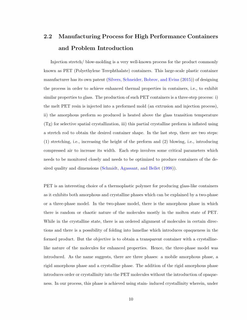
Injection stretch/ blow-molding is a very well-known process for the product commonly

known as PET (Polyethylene Terephthalate) containers. This large-scale plastic container

manufacturer has its own patent (Silvers, Schneider, Bobrov, and Evins (2015)) of designing

the process in order to achieve enhanced thermal properties in containers, i.e., to exhibit

similar properties to glass. The production of such PET containers is a three-step process: i)

the melt PET resin is injected into a preformed mold (an extrusion and injection process),

ii) the amorphous preform so produced is heated above the glass transition temperature

(Tg) for selective spatial crystallization, iii) this partial crystalline preform is inflated using

a stretch rod to obtain the desired container shape. In the last step, there are two steps:

(1) stretching, i.e., increasing the height of the preform and (2) blowing, i.e., introducing

compressed air to increase its width. Each step involves some critical parameters which

needs to be monitored closely and needs to be optimized to produce containers of the de-

sired quality and dimensions (Schmidt, Agassant, and Bellet (1998)).

PET is an interesting choice of a thermoplastic polymer for producing glass-like containers

as it exhibits both amorphous and crystalline phases which can be explained by a two-phase

or a three-phase model. In the two-phase model, there is the amorphous phase in which

there is random or chaotic nature of the molecules mostly in the molten state of PET.

While in the crystalline state, there is an ordered alignment of molecules in certain direc-

tions and there is a possibility of folding into lamellae which introduces opaqueness in the

formed product. But the objective is to obtain a transparent container with a crystalline-

like nature of the molecules for enhanced properties. Hence, the three-phase model was

introduced. As the name suggests, there are three phases: a mobile amorphous phase, a

rigid amorphous phase and a crystalline phase. The addition of the rigid amorphous phase

introduces order or crystallinity into the PET molecules without the introduction of opaque-

ness. In our process, this phase is achieved using stain- induced crystallinity wherein, under

10

suitable heating and stretching ratios, the molecules are oriented in the desired direction.

The innovation in the process comes from the introduction of a preferential heating process

at preferred locations which is performed to optimize the material distribution and rigid

amorphous phase once stretched and blown. The process parameters, in this case play a

crucial role as there are several metastable states possible (during thermal annealing it can

even reside in a completely crystalline phase or the mobile rigid phase or a combination

of all three) and the process variables have to be optimized to achieve the desired state

wherein the transition to the completely crystalline phase is a very slow process and does

not introduce anomalies like shrinkage once removed from the molds (Silvers et al. (2015)).

PET blow-molding is such a complex and precise process that a deeper understanding,

requiring predictive capability and control, is needed to make sure the produced containers

have the desired shapes and specifications. To accomplish this goal, we started the process

by exploring the data set consisting of sensor signals from various sources, including the

temperatures at the heated zones in the preform, the stretching rod position and speed,

the mold both for preform and container parameters, etc. Then, in order to understand

and quantify the hypothesized correlation between variables, we designed various experi-

ments starting from Aspen Fluent simulations to narrow down the range of the parameters,

single mold experiments with location- mapping to understand the stretch/blow process ,

and lastly experiments in the real-life scenario, i.e., on the production line to characterize

the process noise. After gaining deeper insights and to move from an analytical to a more

predictive approach, we developed Gaussian Bayesian Networks. The following sections

explain the work in more detail.

2.3 Data Collection and Hypothesis Development

The objective of data collection and hypothesis development is to develop analytical ca-

pabilities from the plethora of data collected from multiple sensors on the production line.

The data is stored on a server where the data are aligned in a relational tabular database

11

Figure 2.1: Mean and Standard Deviation trend of the collected thickness data

format, and can be easily extracted through queries written in Python or MySQL. One of

the major output or dependent variables are the produced container specifications in terms

of thickness collected at the end of the process. To start with data exploration, the first task

was to look into the statistical measures of the thickness and process data to observe the

trend and patterns especially at the sensors used as kickout criteria. The objective of this

activity was to make sure the data being collected for multiple containers shows a mean

value close to the desired values with low standard deviation (problems especially came

as each of the 16 container data collected comes from a different cavity in the blow-mold

process). The root cause identification for high standard deviation was the next step either

as measurement noise or process noise. Figure 2.1 shows an example trend in the thickness

mean and standard deviation measurement values at various locations. As we can clearly

see from the plot, those measurements at certain locations like 4 and 6 are too thin, while

those at locations 8 and 12 are too thick. The variation at certain locations like 6, 7, 8

were identified as measurement noise due to the placement of those sensors on the mea-

suring equipment, while those at 1, 2, 10, 11 (critical for kick-out) were due to process noise.

As mentioned before, the aim is to identify process variables which are correlated to thick-

ness measurements (both from a data and physical understanding point of view) in order

12

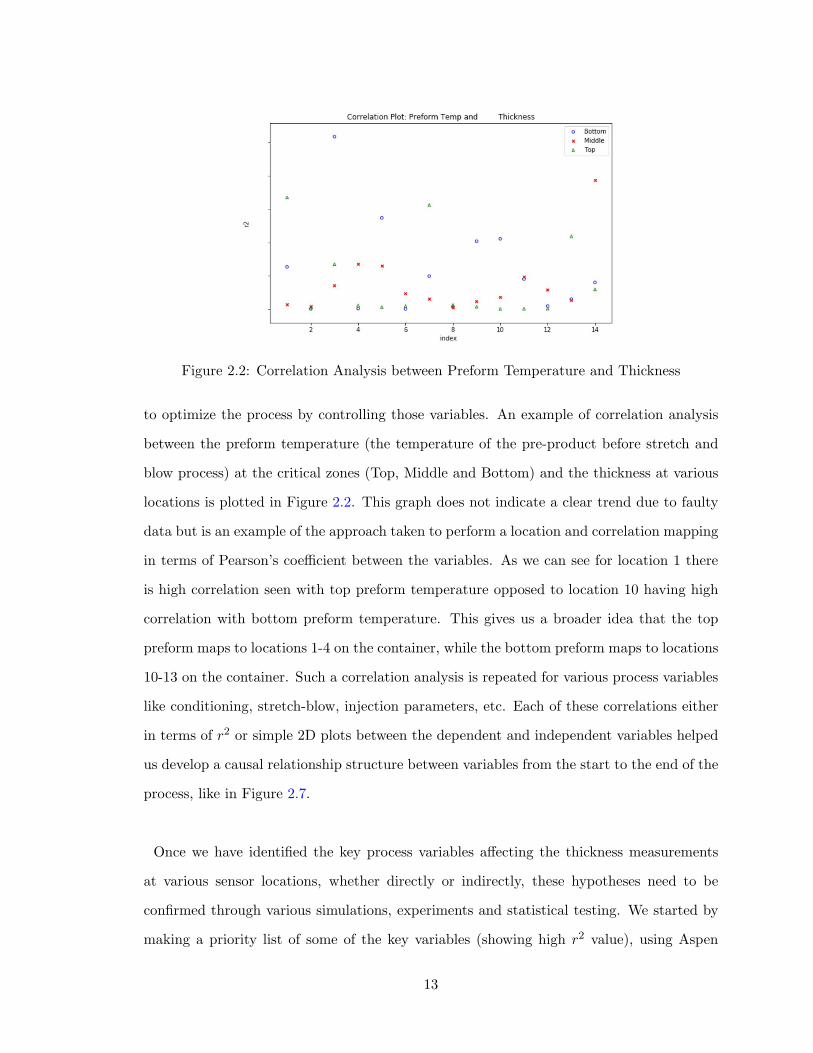
Figure 2.2: Correlation Analysis between Preform Temperature and Thickness

to optimize the process by controlling those variables. An example of correlation analysis

between the preform temperature (the temperature of the pre-product before stretch and

blow process) at the critical zones (Top, Middle and Bottom) and the thickness at various

locations is plotted in Figure 2.2. This graph does not indicate a clear trend due to faulty

data but is an example of the approach taken to perform a location and correlation mapping

in terms of Pearson’s coefficient between the variables. As we can see for location 1 there

is high correlation seen with top preform temperature opposed to location 10 having high

correlation with bottom preform temperature. This gives us a broader idea that the top

preform maps to locations 1-4 on the container, while the bottom preform maps to locations

10-13 on the container. Such a correlation analysis is repeated for various process variables

like conditioning, stretch-blow, injection parameters, etc. Each of these correlations either

in terms of r2 or simple 2D plots between the dependent and independent variables helped

us develop a causal relationship structure between variables from the start to the end of the

process, like in Figure 2.7.

Once we have identified the key process variables affecting the thickness measurements

at various sensor locations, whether directly or indirectly, these hypotheses need to be

confirmed through various simulations, experiments and statistical testing. We started by

making a priority list of some of the key variables (showing high r2 value), using Aspen

13

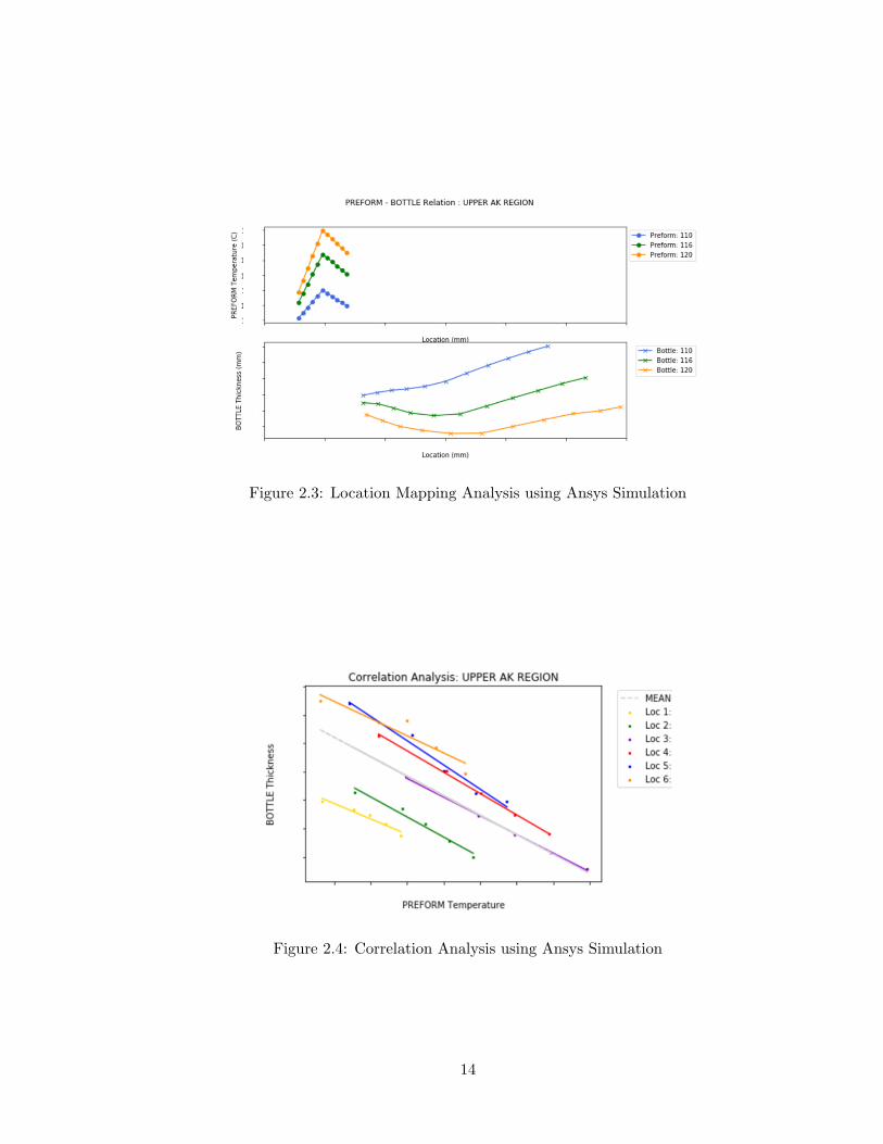
Figure 2.3: Location Mapping Analysis using Ansys Simulation

Figure 2.4: Correlation Analysis using Ansys Simulation

14

simulations to observe the effect of these variables. We also identified a range and step size

for each of the variables where they significantly affect the material distribution, which is

then used for the next few steps of performing experiments and quantifying this relation-

ship through linear/non-linear equations. Through these simulations, we also performed a

theoretical location-mapping to understand where each zone of the preform corresponds to

on the formed container. Figure 2.3 indicates the location-mapping from the preform (top

plot) to the formed bottle (bottom plot), the trend shift on increasing preform temperature

at certain locations shows the material distribution/ expansion once the preform is stretch-

blown. Figure 2.4 shows the correlation analysis between preform temperature and bottle

thickness measurements at various locations together with the mean fitted line to form a

static linear regression model. The results were used for pilot plant studies, where on a

single cavity machine each of the process variables was altered between the range identified

in simulations. The data were collected for the thickness at various locations. In order to

perform location-mapping on a pilot scale, we carried out a UV light ink-jet marking on the

preform (physical marking was not possible as this is a continuous process), the location

and extension of ’I’ or ’T’ marked shape indicates the mapping and extent of the expansion

or contraction on varying the process variables. The data so-collected was cleaned, analyzed

and showed results in accordance with the simulation results (confirmed through a T test, a

statistical technique to accept a null hypothesis in this case as the sample size 30). Figure

2.5 shows an example of the results we obtained. This clearly shows the movement in the

I shape on increasing the preform temperature, thus enhancing the material distribution.

The next step was to confirm these pilot plant studies with the production line where there

is an added complexity of process noise (as this is a continuous process). Similar experi-

ments were repeated on a large scale, where the process variables were varied between the

range identified and the data so-collected were analyzed to develop correlations and static

regression equations which provided an analytical and capability of the process both for

optimization and control. Figure 2.6 shows some of the results of these correlation analysis

through linear plots and sensitivity analysis as a heat map, it clearly indicated a strong re-

lation between the temperatures and a higher sensitivity of the latter to thickness readings

15

Figure 2.5: Location Mapping Analysis through Pilot Plant studies

Figure 2.6: Correlation Analysis through Large Scale studies

from the bottom sensors. But the major disadvantage of these static model equations is

that they fail miserably even if set points are changed for any process variable, or working

with a new product entirely. In such cases, the experiments need to be repeated, which is

both time-consuming and expensive. Hence we need a data-driven model which can retrain

itself every few weeks, thus automating the process modeling. This is discussed in the next

few sections.

2.4 Gaussian Bayesian Networks

As mentioned and derived in the previous sections, the causal relationships between vari-

ables can be verified using statistical testing and modeled using first order linear equations.

But the caveat in this process is that, for any slight change to the process, such experiments

16

have to be repeated. In order to automate this process, and reduce the labor-intensive pro-

cess of conducting experiments, collecting data, performing statistical tests and developing

linear models which are to be utilized by process engineers to optimize and control the pro-

cess, we propose a better strategy to utilize the gigabytes of data being collected everyday

from the processes. Data-driven approaches for the computational modeling of processes

have entered every sector from a simple linear regression between process variables to the

use of neural networks for drug development and many more. Most of these algorithms have

two approaches, either a deterministic route to develop model equations to get the point

estimates, or a probabilistic route to obtain these relationships as probability distributions

which provide point estimates along with a confidence interval. A number of these algo-

rithms take the probabilistic route, like Bayesian Networks (BN). Bayesian Networks are

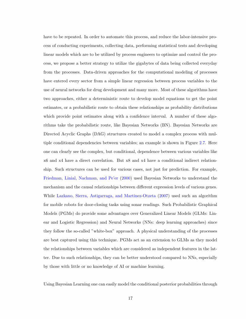
Directed Acyclic Graphs (DAG) structures created to model a complex process with mul-

tiple conditional dependencies between variables; an example is shown in Figure 2.7. Here

one can clearly see the complex, but conditional, dependence between various variables like

x6 and x4 have a direct correlation. But x8 and x4 have a conditional indirect relation-

ship. Such structures can be used for various cases, not just for prediction. For example,

Friedman, Linial, Nachman, and Pe’er (2000) used Bayesian Networks to understand the

mechanism and the causal relationships between different expression levels of various genes.

While Lazkano, Sierra, Astigarraga, and Martinez-Otzeta (2007) used such an algorithm

for mobile robots for door-closing tasks using sonar readings. Such Probabilistic Graphical

Models (PGMs) do provide some advantages over Generalized Linear Models (GLMs: Lin-

ear and Logistic Regression) and Neural Networks (NNs: deep learning approaches) since

they follow the so-called ”white-box” approach. A physical understanding of the processes

are best captured using this technique. PGMs act as an extension to GLMs as they model

the relationships between variables which are considered as independent features in the lat-

ter. Due to such relationships, they can be better understood compared to NNs, especially

by those with little or no knowledge of AI or machine learning.

Using Bayesian Learning one can easily model the conditional posterior probabilities through

17

Figure 2.7: Bayesian Network: Directed Acyclic Graph of 10 nodes

the well-known Bayes Theorem, as listed in Equation 1. Some of the advantages of going

this route are, first, the parametric model is estimated as a likelihood function for a given

variable and data and second it gets updated with more evidence i.e more data being col-

lected. Based on a physical understanding of the process we can make an assumption of

the prior like in this case the Gaussian distribution (most process variables are normally

distributed) or start with no assumption like a Uniform distribution. Each of the edges in

the Bayesian network structure are formed as parent-child relationships and can be drawn

from the various hypothesis and results carried out in Section 2.3, and are modeled as condi-

tional or joint probability distribution for each parent-child edge, while the entire network

is modeled as a joint probability distribution expressed as the product of all conditional

probability distributions as shown in Equation 2.

P (A|B) =P (B|A)P (A)

P (B)(1)

P (X1, X2...Xn) =

n∏i=1

P (i|Par(i)) (2)

Here, the relationships between process variables are modeled as a Bayesian Network struc-

ture connected through conditional probability distributions. Different variables like source

and product temperatures were related through a conditional probability distribution. And

from the results of the analysis of various hypothesis experiments conducted in Section

2.3, we can conclude that each of these probability distributions is a Linear Gaussian

18

Distribution. The expansion of probabilities in Equation 1 are listed in Equations 3 to

4. Additionally, the multivariate joint probability distribution in Equation 2 can be ex-

pressed in terms of mean and co-variance matrix using a simple Gaussian expansion listed

in Equation 5, where p is the number of samples in the data-set. We can clearly observe

from these equations that the point estimates/expected values of the Gaussian distribution

represent a simple linear regression model quite similar to the static model derived in the

previous sections. But the added advantage of this technique is it uses the plethora of data

to fit probability distributions according to the parent-child relationships as described in the

Bayesian Network structure, and uses the fitted model to provide both the expected values

and the 90-95% confidence interval based on the variation requirements. The parametric

model parameters can be easily derived through various mathematical techniques like linear

algebra, discussed more in the next section.

Par(Y ) = X = [X1, X2, X3, ..., Xm] (3)

P (Y |X) = N(β1X + β0, σ2) (4)

P (X1, X2.., Xn) =1

(2π)p/2(Σ)pexp(−

XdiffΣ−1XTdiff

2) (5)

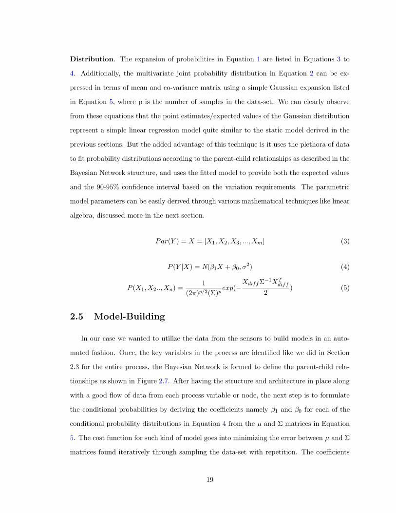
2.5 Model-Building

In our case we wanted to utilize the data from the sensors to build models in an auto-

mated fashion. Once, the key variables in the process are identified like we did in Section

2.3 for the entire process, the Bayesian Network is formed to define the parent-child rela-

tionships as shown in Figure 2.7. After having the structure and architecture in place along

with a good flow of data from each process variable or node, the next step is to formulate

the conditional probabilities by deriving the coefficients namely β1 and β0 for each of the

conditional probability distributions in Equation 4 from the µ and Σ matrices in Equation

5. The cost function for such kind of model goes into minimizing the error between µ and Σ

matrices found iteratively through sampling the data-set with repetition. The coefficients

19

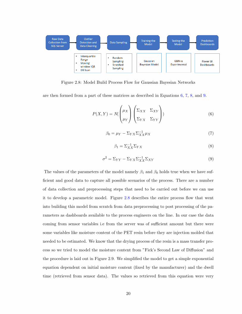
Figure 2.8: Model Build Process Flow for Gaussian Bayesian Networks

are then formed from a part of these matrices as described in Equations 6, 7, 8, and 9.

P (X,Y ) = N(

µXµY

ΣXX ΣXY

ΣY X ΣY Y

) (6)

β0 = µY − ΣY XΣ−1XXµX (7)

β1 = Σ−1XXΣY X (8)

σ2 = ΣY Y − ΣY XΣ−1XXΣXY (9)

The values of the parameters of the model namely β1 and β0 holds true when we have suf-

ficient and good data to capture all possible scenarios of the process. There are a number

of data collection and preprocessing steps that need to be carried out before we can use

it to develop a parametric model. Figure 2.8 describes the entire process flow that went

into building this model from scratch from data preprocessing to post processing of the pa-

rameters as dashboards available to the process engineers on the line. In our case the data

coming from sensor variables i.e from the server was of sufficient amount but there were

some variables like moisture content of the PET resin before they are injection molded that

needed to be estimated. We know that the drying process of the resin is a mass transfer pro-

cess so we tried to model the moisture content from ”Fick’s Second Law of Diffusion” and

the procedure is laid out in Figure 2.9. We simplified the model to get a simple exponential

equation dependent on initial moisture content (fixed by the manufacturer) and the dwell

time (retrieved from sensor data). The values so retrieved from this equation were very

20

Figure 2.9: Moisture Content Estimation Procedure

close to experimentally determined values of moisture content, it was then preprocessed

and fed to the model to develop the Gaussian Bayesian Network.

After data for all the variables in Bayesian Network Structure is retrieved, the next

step is to clean the data of any outliers but to make sure we have enough range in the data

to make high confidence estimates. We tried various outlier detection algorithms to clean

the data-set, they varied in their technique and the variable they were applied to. One of

the novel approaches we used was a ”Rolling Window Inter Quartile Range Filter”. As the

distribution of the data is assumed to be Normal/Gaussian, a outlier is defined as point

which is outside the 1.5 ∗ IQR window. This is a standard IQR approach for outliers, but

here we make IQR as a moving window filter as the set-points of variables are continu-

ously varying thus having a fixed value can result in a number of false positives/negatives.

Figure 2.10 shows this approach using an example data set and the predicted outliers are

indicated as false positives/negatives in the second sub-plot. As we can observe that us-

ing this approach the number of FP/FN are kept to a minimum even with the change in

the set-point of the variable which might not be fully captured by a standard IQR approach.

21

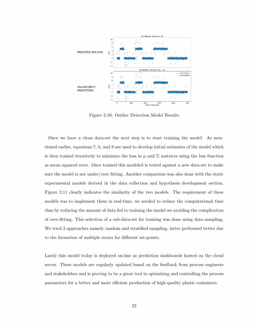
Figure 2.10: Outlier Detection Model Results

Once we have a clean data-set the next step is to start training the model. As men-

tioned earlier, equations 7, 8, and 9 are used to develop initial estimates of the model which

is then trained iteratively to minimize the loss in µ and Σ matrices using the loss function

as mean squared error. Once trained this modeled is tested against a new data-set to make

sure the model is not under/over fitting. Another comparison was also done with the static

experimental models derived in the data collection and hypothesis development section.

Figure 2.11 clearly indicates the similarity of the two models. The requirement of these

models was to implement them in real-time, we needed to reduce the computational time

thus by reducing the amount of data fed to training the model we avoiding the complication

of over-fitting. This selection of a sub-data-set for training was done using data sampling.

We tried 2 approaches namely random and stratified sampling, latter performed better due

to the formation of multiple strata for different set-points.

Lastly this model today is deployed on-line as prediction dashboards hosted on the cloud

server. These models are regularly updated based on the feedback from process engineers

and stakeholders and is proving to be a great tool in optimizing and controlling the process

parameters for a better and more efficient production of high-quality plastic containers.

22

Figure 2.11: Comparison of Experimental and Data Driven Model

2.6 Extension to Root Cause Analysis

Our next aim to enhance the predictive capabilities of the process, not only for process

optimization and control, is to build fault detection and root cause analysis algorithm.

Imagine if a fault occurs in the process. First, we need to detect it from the data using the

joint probability distribution we estimated in the previous section. We also need to identify

the root cause and the pathway using the Bayesian network structure and the “parent-child”

relationships, as shown in Figure 2.7. The work for this algorithm is in process and has not

been finalized yet.

23

Chapter 3

Inline Quality Control using

Computer Vision Tools

3.1 Introduction

In order to meet the increasing demand, most manufacturing sectors have developed

processes with high yields using state of the art technology, as described in the previous

chapter. But product consistency also has to be maintained; this requires a more efficient

process and faster quality control (QC). QC is one of the vital parts of the process, especially

for a multi-stage production system. Often, QC is done manually on the line by picking

up random samples and performing certain listed tests on the products. More traditional

techniques include the use of Statistical Quality Control Charts on the line, as shown in

Godina, Matias, Azevedo, et al. (2016). Decisions regarding the quality of the manufactured

products are made using various plots of the statistical measures, like x-bar and standard

deviation. In the age of digitization to reduce human effort, several new techniques have

been proposed. For example, Rocha, Peres, Barata, Barbosa, and Leitao (2018) propose

an automated ML model to construct decision-rules regarding the quality of the product

with minimum human intervention. This chapter describes another interesting approach

towards this goal: Inline quality control of the product specifically to identify a good vs. bad

product, based on residual stress profiles using a state of the art computer vision technique

24

named “convolution neural networks.” Each section in here describes the theory and the

methodology followed for this project.

3.2 Photo-Elasticity Measurements

PET containers are polymer-based products exhibiting residual stresses due to the in-

jection molding process by which they are formed. These residual stress patterns can be

used to identify the strength of the product, especially to estimate the probability of the

resultant blow-molded bottle being defective. A common technique is to observe residual

stress patterns, i.e., the stress remaining in the material after external forces are applied.

In this case, the injection molding represents the external force. To maintain mechanical

equilibrium in the product such residual stresses can be generated; these can be used to

classify the product as good or defective. But these residual stress patterns are not visible

with the naked eye, and require an optical technique to view these trends. A well-known

technique, ”birefringence” or ”photo-elasticity,” can quantify the optical quality of the sub-

stance in the form of an image (Aben, Ainola, and Anton (2000)).In this method, the stress

fields are visible when a monochromatic light is passed through a material (photosensitive

containing the residual stresses). This resolves the light into two components with different

refractive indices (hence the name double/bi-refraction). The difference in the refractive

indices creates a phase difference between the two components, which then creates a fringe

pattern which can be correctly captured through a camera/sensor. The equations listed

below are an optics law (Equation 10) and fringe equations (Equation 11) that correctly

quantify such phenomena in terms of phase retardation and the number of fringes in the

pattern (Noyan and Cohen (2013)). It can be observed from these equations that N and ∆

are dependent on t, the thickness of the photosensitive material. It is observed in our case

that a good pre-product within the desired specification range produces a uniform residual

stress birefringence pattern. In contracts, a defective one produces different kinds of random

patterns, dependent on how much the thickness varies from the desired specifications.

25

∆ =2πt

λC(σ1 − σ2) (10)

N =∆

2π(11)

3.3 Experimental Setup

The objective of the photo-elasticity experiments was to create a data-set for all residual

stress profile images of the products, which will be further input fed to a computer vision

algorithm for classification. In this data-set there are changes in the residual stress profile

pattern as we shift from good (uniform) to a defective product (disoriented). In order to get

the data-set for such residual pattern images, 350 good and defective products were collected

from the production line. Each of the collected products was placed on a customized holder

and photo-elastic measurement technique, as described in the above section was used to

visualize the residual stress pattern. The holder with the product was placed between the

light source and camera with the polarizer film to generate a monochromatic light from the

white light source, as shown in Figure 3.1. The received image were the residual patterns

and the process was repeated for all the collected products, good or bad. The obtained

image data set was then pre-processed and fed to the classification algorithm for in-line

quality control.

3.4 Convolution Neural Networks

As for the classification task to identify the product good or defective from residual

stress patterns, we use a state of the art computer vision technique in deep learning known

as ”Convolution Neural Networks” (CNN). CNNs are advanced neural networks to handle

2D/3D, more specifically image data. The concept of neural networks was inspired from

biology, specifically the nervous system (connection of neurons) in our body, in which each

of the neurons perform a simple task of passing the messages, but the network overall can

26

Figure 3.1: Experimental Setup for Photo-elasticity measurement for visualizing residualstress patterns

perform complex and multiple tasks like running, reflex actions, etc. Similarly, a ”Per-

ceptron” or a single-layered neural network, utilizes the combinatory power of individual

neurons performing simple functions, like the evaluation of a non-linear function over a lin-

ear combination of input features (Figure 3.2 ). CNNs are an extension to neural networks

where, in instead of multiple neurons for an initial few layers in the network, there is a

kernel of a certain size which performs the convolutional operation over the input image (a

2D/3D matrix of pixel intensity values). This convolutional operation can be compared to

a “moving dot product” operation between matrices. This is a repetitive operation between

the kernel matrix and a part of the image matrix of the same size as the kernel, which

results in another matrix of a different size. CNNs are preferred over Neural Networks as

they involve fewer parameters to learn/fit the model. This is especially helpful when the

input feature size is huge (each pixel can be considered as a feature). This approach makes

the model training process faster, especially for large images. A simple convolution neural

network for a binary classification task is depicted in Figure 3.3. O’Shea and Nash (2015)

tdiscuss how the number of parameters that have to be learnt increases exponentially for

a NN when training over image data, especially with RGB (red/green/blue) images. Thus,

a CNN approach has a great advantage over a NN since, irrespective of the image size,

the kernel size for the convolution operation over the image data set remains constant with

increase in the image size, thus limiting the number of weights that need to be learnt.

27

Figure 3.2: A Simple 2 Layer Neural Network Explanation

As CNNs are inspired by NNs, their training, i.e., the forward and backward propagation,

is very similar to that of a neural network. The weights and biases in a neural network are

the parameters of the model which have to be learnt through the data used for training such

a model. The learning aspects of these networks happen during the backward propagation

where the objective is to find the optimal choice of weights and bias for each neuron in each

layer which minimizes the cost function (the sum of errors between the actual and predicted

values). Every image/ data point fed to such network structures moves the weights and bias

towards the optimal value one step at a time using an iterative approach commonly known

as “gradient descent”. While building the model for a specific application, the architecture,

the loss function, optimizer algorithm, and non-linearity component have to be tuned in

order to minimize the error. The next section describes the model build, data preprocessing,

hyperparameter tuning and evaluation techniques we used for our CNN model to perform

the classification task on the image data set collected from the photo-elasticity experiments.

3.5 Model Building

The initial CNN Model Architecture was inspired by a simple “dog-cat” image classifier,

well-known in the deep learning sector. But before getting into the model architecture and

28

Figure 3.3: Convolution Neural Network Model for Binary Classification

training, the image data-set needed to be preprocessed to avoid under- or ove-r fitting of

the model (one of the most common problems in machine learning). The requirement from

the model is that it should perform well on the data fed to it (to avoid under-fitting), but

be generalized enough to still perform well on new input data (to avoid over-fitting). There

were 700 images collected (good and bad) through the experiments conducted in Section

3.3. We use this data for three tasks: training the model to learn the weights and biases,

validate the model for hyper-parameter tuning (like architecture, loss, optimizer, etc.), and,

lastly, test the model on a new data-set. As the image data-set was limited, the validation

data-set for hyper-parameter tuning and test data-set for testing the model was restricted

to 200 images combined. In the training data-set, there were 225 good and 225 bad images.

Each of these images was binary-labeled (0 for good and 1 for bad), resized to a shape of

120*120 (height x width) (found as the optimum size, neither under- nor over- fitted) and

gray-scaled to reduce the complexity of multiple color channels.

The CNN model architecture was finalized to have Convolution and Max-Pool (size re-

duction) Layers with a kernel size of 3*3, in order to create a feature map. This is a grid

map of the input image containing all the characteristic features, which can very well clas-

sify the product, for the photo-elastic images. These stacked-up layers were followed by

a flattening layer to convert from 2D to 1D input vectors. Further followed by the fully

connected layer before final output layer to extract essential components as a single vector

from this feature map in order classify the images. In the output layer, using a sigmoid

29

Figure 3.4: Training and Validation Loss and Accuracy curves

as the activation function (the non linear function the neuron applied on the linear com-

bination of the input features), we obtain a single value indicating the probability for the

product to be defective. As probability values lie in the range of 0 and 1, we chose 0.5

as the threshold. Values above this would be classified as defective or labeled as 1. The

model was trained using the preprocessed training data-set and, as mentioned in the pre-

vious section, the weights were learnt using backward propagation., Here the loss function

was set as the binary cross entropy loss described in Equation 12, commonly used for such

binary classification tasks. The hyper-parameters included the kernel size, number of nodes

in the fully connected layer, the optimizer algorithm, number of iterations for the gradient

descent algorithm, etc. These hyper-parameters were tuned by observing the validation and

training losses, as shown in Figure 3.5. Finally, the model was tested using the test data-set

and the results are described in the next section.

L =

n∑i=1

(yilog(h(xi)) + (1− yi)log(1− h(xi))) (12)

30

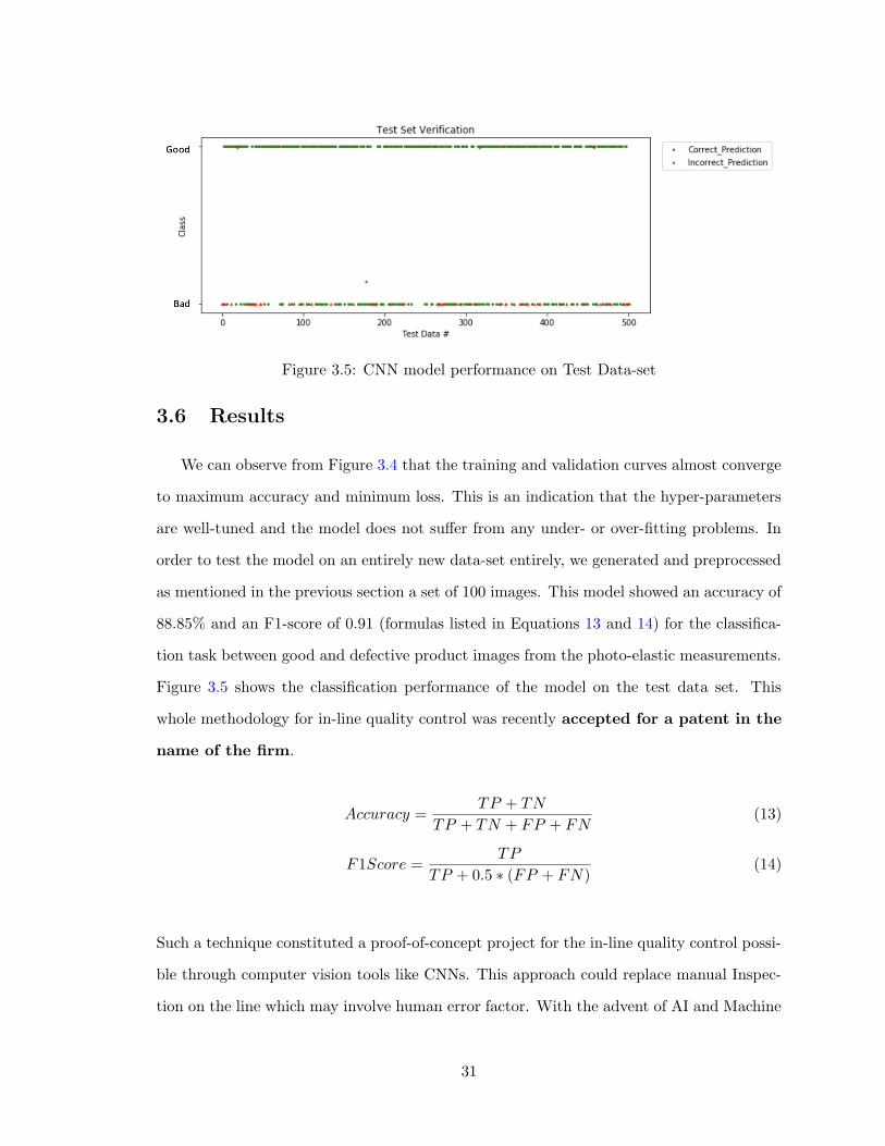
Figure 3.5: CNN model performance on Test Data-set

3.6 Results

We can observe from Figure 3.4 that the training and validation curves almost converge

to maximum accuracy and minimum loss. This is an indication that the hyper-parameters

are well-tuned and the model does not suffer from any under- or over-fitting problems. In

order to test the model on an entirely new data-set entirely, we generated and preprocessed

as mentioned in the previous section a set of 100 images. This model showed an accuracy of

88.85% and an F1-score of 0.91 (formulas listed in Equations 13 and 14) for the classifica-

tion task between good and defective product images from the photo-elastic measurements.

Figure 3.5 shows the classification performance of the model on the test data set. This

whole methodology for in-line quality control was recently accepted for a patent in the

name of the firm.

Accuracy =TP + TN

TP + TN + FP + FN(13)

F1Score =TP

TP + 0.5 ∗ (FP + FN)(14)

Such a technique constituted a proof-of-concept project for the in-line quality control possi-

ble through computer vision tools like CNNs. This approach could replace manual Inspec-

tion on the line which may involve human error factor. With the advent of AI and Machine

31

Learning, a number of firms are moving towards automating the process of visual inspection

and making the process more robust by decreasing the number of false positives/negatives

using such techniques. With the increase in demand of the products, manufacturing firms

are trying their best to fasten the production as well as quality control process, there is

an urgent need for such tools as manual inspection is physically impossible if the line runs

at a high speeds and produces a large quantity of products. Industries like automotive

and semiconductor have already adapted such tools as part of Industry 4.0, and increasing

number of firms are realizing the importance to use such data driven tools to automate and

improve their processes.

32

Chapter 4

Predictive Maintenance using

Machine Learning

4.1 Introduction

In most industries, maintenance is one of the biggest reasons to shut down a production

line. This plays a considerable role in lost production. Randomly occurring failures are

hard to locate and time-consuming to resolve, this is the Run to Failure (R2F) strategy.

To avoid this, often plants follow a Preventive Maintenance (PvM) strategy where a main-

tenance procedure for all equipments is scheduled every other week or fortnight based on

the equipment. This has an added advantage over R2F as this ensures that each equipment

is performing as desired. Often this leads to additional maintenance, even when not re-

quired, as the time interval between procedures is hard to estimate. In some cases, it incurs

additional costs over R2F. especially for expensive and complex machines which have a

time-consuming and costly maintenance procedure.

AAnother approach is Predictive Maintenance (Pdm) in which the strategy is to use sen-

sor data to predict failure occurrence and schedule maintenance procedures accordingly.

This is based on Remaining Useful Life (RUL) predictions, i.e., the time left before the

equipment fails. Such a strategy minimizes maintenance costs and production losses, as

well as maximizing equipment life. There are multiple ways to pursue PdM as a part of

33

Industry 4.0 and one of the methods which is being adopted rapidly by various industries

(as mentioned in Chapter 1) is a data-driven strategy. There are many possible algorithms;

the choice and parameter-tuning of such tools are problem/ situation-specific. With such

a data-integrative approach, machine downtime can be reduced, making it easier to find

the root cause, with cost-savings and reduced as well as increasing the efficiency of the

equipment (Carvalho et al. (2019)).

There are two approaches to an ML-driven PdM that include supervised and unsupervised

learning. The former requires a large historical labeled data-set, with different cases of

failures on the machines. This is similar to the approach seen in Chapter 3, trends/patterns

in sensor data can be identified to predict the remaining useful life, helping to determine

when failure is likely to occur. The latter approach tries to find trends in the data without

historical knowledge of the failures. Either of the two approaches can be chosen based on a

number of factors, like the availability of historical data, a trade-off between efficiency and

accuracy, etc. There are a number of algorithms to tackle this, each with its own pros and

cons (Paolanti et al. (2018)).

The problem statement provided to us was to develop a PdM strategy for the process

modeled in Chapter 2. We started by analyzing the downtime and maintenance cost per

equipment (manually) in the process for the production of high efficiency plastic containers.

We also met with operators and process engineers to understand their view point based

on years of experience supervising the machine. The two major bottlenecks we uncovered

involved mechanical and thermal equipment; both of which had long down-times and high

occurrence. The PdM approach for such equipment included analyzing the vibrational sig-

nals from the equipment (mechanical) or temperature and pressure sensor data (thermal

equipment). This was followed by developing models to predict failures in each case, hence

developing a predictive capability for scheduling maintenance procedures. Section 4.2 de-

scribes supervised approach in detail with proof of concept examples. Section 4.3 describes

an unsupervised approach often used in natural language processing problems. Using the

34

human-recorded maintenance dispatch history data on the line, our goal was to identify

the root cause component, which had the highest occurrence, and large downtime during

the preceding 6-12 months. . This chapter describes several approaches to utilize machine

learning in predictive maintenance and root cause identification as a PdM strategy for a

given process.

4.2 Predictive Maintenance using Sensor Data

In this section, predictive maintenance is carried out through condition-based mainte-

nance. Hashemian (2010) explains different state-of the art approaches to develop a PdM

strategy for sensor data from mechanical components, like vibrational amplitude signals,

or thermal components, like thermocouple and pressure data. The three projects used a

correlation analysis between variables as well as feature identification for a complete condi-

tion monitoring of the equipment. Kaiser and Gebraeel (2009) depict the latter approach

in a different way by utilizing the sensor variable degradation patterns to provide a better

estimate of remaining useful life of the equipment in a more real-time fashion by a feedback

loop technique. Depending on this estimate, the proposed algorithm also provides a better

suggestion for scheduled maintenance compared to conventional techniques. Inspired by

these strategies, we propose similar PdM strategies for our problem statement.

As mentioned in the previous section, the two bottlenecks identified involved mechani-

cal and thermal equipment. Predictive maintenance for these two cases was carried out as

separate tasks, first fault diagnosis using the vibrational signals on mechanical equipment

and using sensor data for predictions of Remaining Useful Life. Both these examples were

carried out as proof of concept projects using small data-sets which are then implemented

for larger-scale scenarios in the plant.

35

4.2.1 Approach 1: Fault Diagnostics

For mechanical equipment, one of the major tasks is to identify if a fault has occurred

at an early enough stage, before it undergoes permanent damage. Here, we have a time-

dependent vibrational signal from the equipment. Our proposed strategy for fault diag-

nostics is to identify these faults by analyzing data in a different domain than time. So

the first step is to convert the data from a time to a frequency domain using Fast Fourier

Transform. Figure 4.1 shows the transformation both for normal and faulty signals. Fast

Fourier Transform (FFT) of this data makes the identification of faults easier through peak

identification. FFT algorithms are quite well known especially in computational simulations

or signal processing to perform discrete Fourier transforms or inverse discrete Fourier trans-

forms at a faster rate by reducing the complexity of algorithms from O(N2) to O(Nlog(N))

(Cochran et al. (1967)). Our approach includes converting signals from a time domain to

a frequency domain and then performing peak identification using a classification machine

learning algorithm. As indicated before, this is a “supervised” approach, which requires

significant historically labeled data. This algorithm, once trained, is fed frequency domain

data continuously, or in real-time, and can detect whether the machine state is ‘normal’

or ‘abnormal.’ It used fault identification/labeling to determine specific concerns, e.g., a

bearing issue, or mechanical loosening, etc. we could not model this scenario due to lack

of an historically labeled data-set. But such an approach for vibrational signal analysis is

simple and has immense potential to show good accuracy in real-time classification/ fault

diagnostics.

4.2.2 Approach 2: Remaining Useful Life Prediction

For thermal equipment, we have sensor-based data arising from variables such as tem-

perature, pressure, speed, etc. The objective is not only to correctly estimate the fault by

looking at sensor degradation patterns, but also to provide a good estimate of remaining

useful life. Here, we start with labeled data-sets with different failure scenarios and hence

different cases of remaining useful life for the equipment. The objective is achieved by

36

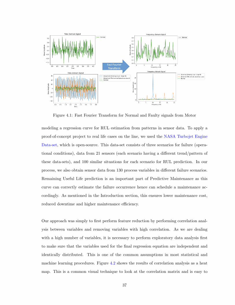
Figure 4.1: Fast Fourier Transform for Normal and Faulty signals from Motor

modeling a regression curve for RUL estimation from patterns in sensor data. To apply a

proof-of-concept project to real life cases on the line, we used the NASA Turbojet Engine

Data-set, which is open-source. This data-set consists of three scenarios for failure (opera-

tional conditions), data from 21 sensors (each scenario having a different trend/pattern of

these data-sets), and 100 similar situations for each scenario for RUL prediction. In our

process, we also obtain sensor data from 130 process variables in different failure scenarios.

Remaining Useful Life prediction is an important part of Predictive Maintenance as this

curve can correctly estimate the failure occurrence hence can schedule a maintenance ac-

cordingly. As mentioned in the Introduction section, this ensures lower maintenance cost,

reduced downtime and higher maintenance efficiency.

Our approach was simply to first perform feature reduction by performing correlation anal-

ysis between variables and removing variables with high correlation. As we are dealing

with a high number of variables, it is necessary to perform exploratory data analysis first

to make sure that the variables used for the final regression equation are independent and

identically distributed. This is one of the common assumptions in most statistical and

machine learning procedures. Figure 4.2 shows the results of correlation analysis as a heat

map. This is a common visual technique to look at the correlation matrix and is easy to

37

Figure 4.2: Correlation Matrix Heat-Map between sensor variable for the Turbojet Engine

interpret. There are some variables which are highly negatively correlated (the second last

two rows/columns), thus a linear combination or one of them can be used in the list of final

model features. Even after this initial analysis, the number of variables remains large (20+

features) for a simple polynomial regression curve. Thus, we use Principal Component Anal-

ysis to reduce the number of variables to its principal components (namely PC1 showing

75% variance) representing linear combinations of variables. This is a common dimension-

ality reduction technique in statistics and machine learning. It works on the principle of

deriving the principal components as eigenvectors and eigenvalues, common linear algebraic

methods. The variance percentage of each principal component indicates how well that PC

can explain or quantify the variance in the data as a linear combination of features. There

are other techniques for dimensionality reduction but this is often a better starting point

one that is well understood and established. The derived principal components (chosen

just the first to show the concept) are then related to the RUL from the labeled data-set

by curve fitting. In this case, we use an exponential curve fit, as seen in Figure 4.3). The

found equation can then be used to predict RUL based on the value of PC1 from the sensor

data received Other PC components may provide a better estimation. Figure 4.3shows the

PCA/curve fitting studies performed with this data-set. This clearly indicates how utilizing

data from sensors interpreted as principal components can fit the noise data for RUL well,

hence enhancing the predictive maintenance power on the line.

38

Figure 4.3: Curve Fitting between the Principle Component and RUL

4.3 Predictive Maintenance using Human Recorded Data

This work was carried out as an exploratory project to utilize human recorded data ,in

this case maintenance records (maintenance dispatch histories) on the line. The objective of

the activity was to find which component fails frequently. The data-set came from software

used on the line to record the maintenance history as “dispatches.” This data-set consists

of several columns ranging from the ID, the person responsible or tackling the maintenance

requirement/fault, comments about the fault, downtime, actions taken to resolve the issue,

etc. The fault can be easily identified if a person goes through the excel sheet and reads the

comments about the fault. But to automate such a process, we require a more aggressive

approach. Such kind of textual analysis techniques are quite common in natural language

processing (NLP) problems and often used in web-scrapping projects. Our approach was to

use the downtime and the comments about the fault along with this technique to develop

a meaningful insight about a component which fails frequently and results in a significant

downtime.

There is a technique in NLP for textual data vectorization called ”TFIDF”: Term Fre-

quency Inverse Document Frequency. All machine learning models accept data in a nu-

meric format, hence it is critical to convert text data into float or integer format. Often

the frequency of words in a sentence is a good approach for this task. One of the simplest

techniques is a ”Count Vectorizer” which is a Boolean conversion. It is ’1’ if a word is

39

Figure 4.4: TFIDF Score calculation on Human Recorded Data for PdM

present in the sentence, else ’0’. This limits the range of the data and takes a lot of memory

space to store such frequencies. TFIDF approach vectorizes the textual data by calculating

the TFIDF score using Equation 15 and 16, where t, d, n are the term, document, and

number of documents, respectively. Such a TFIDF score was calculated for various “words”

in the document (meaning comments from the maintenance records). This follows cleaning

the data-set from “stop words” in English like “a, an , the, and, between”, etc. Figure 4.4

clearly shows an example of the scores and the major component identified for predictive

maintenance. The component identified by a simple frequency count identified the faulty

component under a general category called ”component” which was better analyzed through

comments and the TFIDF scores. This approach identified the molds as the troublesome

component. This was also confirmed by process engineers on the line which have years of

experience with the machine. A plan was proposed to apply the Pdm strategy proposed in

Section 4.2.2 to utilize all the sensor variable data coming from ”molds” to provide a good

estimate of the remaining useful life as well as develop a scheduled maintenance accordingly.

PdM on this component was not carried out due to a lack of data, resources and time.

But the results in this chapter shows the considerable potential in this sector for its appli-

cation, a plan to follow to approach the required goal as well as proof that such techniques

work and can lead to minimized maintenance costs and reduced downtime on the line.

TFIDF = TF (t, d) ∗ IDF (t, d, n) (15)

40

IDF (t, d, n) = log(1 + n

1 +DF (d, t)) + 1 (16)

41

Chapter 5

Summary and Future Work

5.1 Summary

Time consuming manual tasks like approving orders, optimizing a manufacturing pro-

cess for better production, updating documents, etc. are getting more difficult. In recent

years, the world is moving towards automated processes like a database for organizing data

as a structured collection, scheduling procedures and meetings, or just running a simple

program to add 2 numbers. As mentioned in Chapter 1, we are observing a data explosion

which has motivated process industries, like manufacturing plants, to use these data to

reduce the human load. This leads to increasing efficiency and productivity, and eventually

minimizing manufacturing costs leading to higher profits. Chapter 1 also laid out various

case studies where different industries are utilizing the power of data analytical platforms

(IIOT), taking a step towards digital transformation. There were three main things sum-

marized in this chapter as part of the Internet of Things, namely Digital Twin, Automated

Quality Control, and Predictive Maintenance. In the next three chapters, we explained the

theory behind each of these concepts and our work towards this.

Chapter 2 described our work towards developing analytical and predictive capabilities

for a manufacturing process for the production of high performance containers. The ob-

jective was to gain a deeper understanding of the complex process with data coming from

42

multiple sensors, to develop a hypothesis for causal relationships between variables, and to

prove the hypothesis through a series of experiments and statistical testing. We also devel-

oped static model equations to provide analytical and predictive capabilities to the process.

We deployed an automatic technique called Gaussian Bayesian Networks, a probabilistic

method to quantify the relationships between variables for process modeling, optimization

and control. Predictions from this model closely resembled the results from experiments

carried out on the production line, thus developing a ”Digital Twin” of the process.

Chapter 3 provided a proof-of-concept project for automated quality control using com-

puter vision techniques. It described the theory behind the photo-elasticity experiments

carried out for data collection as well as the Convolutional Neural Network model used for

a binary classification task as good/bad products. We achieved an 88.9% accuracy using

this approach. Recently this project was accepted for a patent application by the company.

Continuing the path of digital transformation, Chapter 4 describes the advantage of Predic-

tive Maintenance over React to Failure or Preventive Maintenance both for minimizing the

costs for maintenance and downtime as well as providing the process engineers on the line

the capability to predict failures. Here we described a few proof-of-concept projects to em-

phasize the power of this technique by utilizing the data from sensors or vibrational signals

on mechanical equipment, as well as using data recorded by personnel, e.g., maintenance

records, to predict the trend of failed components.

5.2 Future Work

Our work here is just a small step towards achieving “Industry 4.0” in the manufacturing

sector. There is still a lot of scope for the improvement of these models like increasing

the accuracy of these models, expanding its application to other sectors, exploring new

problems which can be resolved through data driven tools and trying out new state-of the

art techniques for a faster and better prediction. As mentioned in Chapter 2, we have a

Bayesian Network structure in place with causal relationships between variables, this can

43

act as a foundation over which multiple other algorithms like fault detection and root cause

algorithm can be built. We have tried one simple approach towards this task by utilizing

the co-variance matrix but has its own limitations which can be resolved with utilizing

more advanced techniques like Neural Networks. We are in the process of developing such

an approach. Furthermore, the convolutional neural network used in Chapter 3 is a simple

architecture consisting of a few layers. We can further increase the accuracy by building a

deeper network or hyper-tuning the parameters further with a larger image data-set. This

was not possible due to data limitations. But once this is deployed on-line we can generate

sufficient images to continuously improve the model, even with new changes to the faulty

residual patterns. Lastly, predictive maintenance is a time-consuming task with multiple

potential areas for improvement. We proposed a few strategies with very simple examples

which are implemented in real-time. If enough funding and data are available, these tools

can be implemented as a product capable of handling multiple tasks from data collection

to dashboards providing process engineers and operators various insightful results, similar

to the work carried out in Chapter 2. Moreover, research in this area is still nascent, with

new machine and deep learning techniques, like the use of Reinforcement Learning, Auto-

Encoders, etc. These algorithms are being developed and modified every few months. They

will provide us with new ways to tackle the problem of PdM, as well as equipping us with

a continuous strategy for improving model accuracy. We have barely scratched the surface

of Industry 4.0, with considerable possibilities of using new technology in an increasingly

data-driven world. There is a lot of ground left to explore!

44

References

Aben, H., Ainola, L., & Anton, J. (2000). Integrated photoelasticity for nondestructive

residual stress measurement in glass. Optics and lasers in engineering , 33 (1), 49–64.

AI, C. (n.d.). C3ai crm manufacturing platform. , https://c3.ai/products/c3-ai-crm/mfg/.

Albers, A., Gladysz, B., Pinner, T., Butenko, V., & Sturmlinger, T. (2016). Procedure

for defining the system of objectives in the initial phase of an industry 4.0 project

focusing on intelligent quality control systems. Procedia Cirp, 52 , 262–267.

Bahlmann, C., Heidemann, G., & Ritter, H. (1999). Artificial neural networks for automated

quality control of textile seams. Pattern recognition, 32 (6), 1049–1060.

Carvalho, T. P., Soares, F. A., Vita, R., Francisco, R. d. P., Basto, J. P., & Alcala, S. G.

(2019). A systematic literature review of machine learning methods applied to pre-

dictive maintenance. Computers & Industrial Engineering , 137 , 106024.

Cochran, W. T., Cooley, J. W., Favin, D. L., Helms, H. D., Kaenel, R. A., Lang, W. W., . . .

Welch, P. D. (1967). What is the fast fourier transform? Proceedings of the IEEE ,

55 (10), 1664-1674.

Digital, G. (n.d.). Ge predix: Asset performance management system. ,

https://www.ge.com/digital/applications/asset-performance-management.

Digital, S. (n.d.). Digital twin. , https://new.siemens.com/global/en/company/stories/research-

technologies/digitaltwin/digital-twin.html.

Falkonry. (n.d.). Ai based platform for plant operations by falkonry. ,

https://falkonry.com/.

Friedman, N., Linial, M., Nachman, I., & Pe’er, D. (2000). Using bayesian networks to

45

analyze expression data. Journal of computational biology , 7 (3-4), 601–620.

Godina, R., Matias, J. C., Azevedo, S. G., et al. (2016). Quality improvement with statis-

tical process control in the automotive industry. International Journal of Industrial

Engineering and Management (IJIEM), 7 (1), 1–8.

Haag, S., & Anderl, R. (2018). Digital twin–proof of concept. Manufacturing Letters , 15 ,

64–66.

Hashemian, H. M. (2010). State-of-the-art predictive maintenance techniques. IEEE Trans-

actions on Instrumentation and measurement , 60 (1), 226–236.

How the port of rotterdam is using ibm digital twin technology to transform itself from the

biggest to the smartest. (2019). IBM Watson, https://www.ibm.com/blogs/internet-

of-things/iot-digital-twin-rotterdam/.

Kaiser, K. A., & Gebraeel, N. Z. (2009). Predictive maintenance management using sensor-

based degradation models. IEEE Transactions on Systems, Man, and Cybernetics-

Part A: Systems and Humans , 39 (4), 840–849.

KPMG. (2020). Lamborghini’s new suv production line digitalized by kpmg. ,

https://home.kpmg/fi/fi/home/Pinnalla/2020/03/lamborghini-new-suv-production-

line-digitized-by-kpmg.html.

Kumar, S., Tiwari, P., & Zymbler, M. (2019). Internet of things is a revolutionary approach

for future technology enhancement: a review. Journal of Big Data, 6 (1), 1–21.

Lazkano, E., Sierra, B., Astigarraga, A., & Martinez-Otzeta, J. M. (2007). On the use of

bayesian networks to develop behaviours for mobile robots. Robotics and Autonomous

Systems , 55 (3), 253–265.

Melo, S. (2020). The future of maintenance: A guide to industry 4.0. My-

DataScope, https://mydatascope.com/blog/en/the-future-of-maintenance-a-guide-to-

industry-4-0/.

Milenkovic, J. (2019). Mind-twisting iot statistics for 2020 – your home is now online.

KommandoTech, https://kommandotech.com/statistics/iot-statistics/.

Munirathinam, S., & Ramadoss, B. (2016). Predictive models for equipment fault detec-

tion in the semiconductor manufacturing process. IACSIT International Journal of

46

Engineering and Technology , 8 (4), 273–285.

Noyan, I. C., & Cohen, J. B. (2013). Residual stress: measurement by diffraction and

interpretation. Springer.

O’Shea, K., & Nash, R. (2015). An introduction to convolutional neural networks. arXiv

preprint arXiv:1511.08458 .

Paolanti, M., Romeo, L., Felicetti, A., Mancini, A., Frontoni, E., & Loncarski, J. (2018).

Machine learning approach for predictive maintenance in industry 4.0. In 2018 14th

ieee/asme international conference on mechatronic and embedded systems and appli-

cations (mesa) (p. 1-6).

Qin, J., Liu, Y., & Grosvenor, R. (2016). A categorical framework of manufacturing for

industry 4.0 and beyond. Procedia cirp, 52 , 173–178.

Rocha, A. D., Peres, R. S., Barata, J., Barbosa, J., & Leitao, P. (2018). Improvement

of multistage quality control through the integration of decision modeling and cyber-

physical production systems. In 2018 international conference on intelligent systems

(is) (pp. 479–484).

Schmidt, F., Agassant, J.-F., & Bellet, M. (1998). Experimental study and numerical

simulation of the injection stretch/blow molding process. Polymer Engineering &

Science, 38 (9), 1399–1412.

Shao, G., & Helu, M. (2020). Framework for a digital twin in manufacturing: Scope and

requirements. Manufacturing Letters , 24 , 105–107.

Silvers, K. W., Schneider, M. D., Bobrov, S. B., & Evins, S. E. (2015, May 5). Pet containers

with enhanced thermal properties and process for making same. Google Patents. (US

Patent 9,023,446)

Watson, I. (n.d.). Internet of things. , https://www.ibm.com/cloud/internet-of-things.

47