BIS Working Papers No 191

Explaining the Level of Credit Spreads: Option-Implied Jump Risk Premia in a Firm Value Model Martijn Cremers, Joost Driessen, Pascal Maenhout, David Weinbaum

November 2005

JEL Classification Numbers: G12, G13 Keywords: Credit spreads, Firm value model, Jump-diffusion model, Option pricing

BIS Working Papers are written by members of the Monetary and Economic Department of the Bank for International Settlements, and from time to time by other economists, and are published by the Bank. The views expressed in them are those of their authors and not necessarily the views of the BIS.

Copies of publications are available from:

Bank for International Settlements Press & Communications CH-4002 Basel, Switzerland E-mail: publications@bis.org

Fax: +41 61 280 9100 and +41 61 280 8100

This publication is available on the BIS website (www.bis.org).

© Bank for International Settlements 2005. All rights reserved. Brief excerpts may be reproduced or translated provided the source is cited.

ISSN 1020-0959 (print)

ISSN 1682-7678 (online)

iii

Foreword

On 9-10 September 2004, the BIS held a workshop on “The pricing of credit risk”. This event brought together central bankers, academics and market practitioners to exchange views on this issue (see the conference programme in this document). This paper was presented at the workshop. The views expressed are those of the author(s) and not those of the BIS.

v

BIS workshop on “The pricing of credit risk”

9-10 September 2004, Basel, Switzerland

Conference programme

Opening remarks

William White, Bank for International Settlements

Paper 1: The credit risk component in corporate spreads and swap spreads

Authors: David Lando, Copenhagen Business School (joint with Peter Feldhütter)

Discussants: Tony Rodrigues, Federal Reserve Bank of New York Etienne Varloot, Citigroup

Paper 2: Default and recovery implicit in the term structure of sovereign CDS spreads

Authors: Ken Singleton, Stanford University (joint with Jun Pan)

Discussants: Naohiko Baba, Bank of Japan Richard Cantor, Moody’s

Paper 3: Valuation of a CDO and a n-th to default CDS without Monte Carlo simulation

Authors: John Hull, University of Toronto (joint with Alan White)

Discussants: Michael Gibson, Federal Reserve Board Dominic O’Kane, Lehman Brothers

Paper 4: The pricing of unexpected credit losses

Authors: Jeffery Amato and Eli Remolona, Bank for International Settlements

Discussants: Jean Helwege, University of Arizona Ken Singleton, Stanford University

Paper 5: Measuring default risk premia from default swap rates and EDFs

Authors: Darrell Duffie, Stanford University (joint with Antje Berndt, Rohan Douglas, Mark Ferguson and David Schranz)

Discussants: Peter Hordahl, European Central Bank Frank Packer, Bank for International Settlements

Paper 6: On the relation between credit spread puzzles and the equity premium puzzle

Authors: Pierre Collin-Dufresne, UC Berkeley (joint with Long Chen and Bob Goldstein)

Discussants: Monika Piazzesi, University of Chicago Jun Yang, Bank of Canada

Paper 7: Explaining the level of credit spreads: option-implied jump risk premia in a firm value model

Authors: Joost Driessen, University of Amsterdam (joint with Martijn Cremers, Pascal Maenhout and David Weinbaum)

Discussants: Varqa Khadem, Lehman Brothers Garry Young, Bank of England

Explaining the Level of Credit Spreads:

Option-Implied Jump Risk Premia in a Firm Value Model∗

Martijn Cremers† Joost Driessen‡ Pascal Maenhout§ David Weinbaum¶

This version: February 2005

First version: August 2004

Abstract

Prices of equity index put options contain information on the price of systematic

downward jump risk. We use a structural jump-diffusion firm value model to assess

the level of credit spreads that is generated by option-implied jump risk premia. In our

compound option pricing model, an equity index option is an option on a portfolio of call

options on the underlying firm values. We calibrate the model parameters to historical

information on default risk, the equity premium and equity return distribution, and

S&P 500 index option prices. Our results show that a model without jumps fails to

fit the equity return distribution and option prices, and generates a low out-of-sample

prediction for credit spreads. Adding jumps and jump risk premia improves the fit of the

model in terms of equity and option characteristics considerably and brings predicted

credit spread levels much closer to observed levels.

∗We thank participants of the BIS workshop on the ‘Pricing of Credit Risk’, September 2004, for helpfulcomments, in particular the discussants Varqa Khadem and Garry Young.

†Yale School of Management, International Center for Finance, Box 20820, 135 Prospect Street, NewHaven, CT 06520. Email: martijn.cremers@yale.edu.

‡University of Amsterdam, Finance Group, Faculty of Economics and Econometrics, Roetersstraat 11,1018 WB Amsterdam, the Netherlands. Email: J.J.A.G.Driessen@uva.nl.

§INSEAD, Finance Department, Boulevard de Constance, 77305 Fontainebleau Cedex, France. Email:pascal.maenhout@insead.edu.

¶Cornell University, Johnson Graduate School of Management, 375 Sage Hall, Ithaca NY 14853-6201.Email: dw85@cornell.edu.

1

Explaining the Level of Credit Spreads:

Option-Implied Jump Risk Premia in a Firm Value Model

Abstract: Prices of equity index put options contain information on the price of sys-

tematic downward jump risk. We use a structural jump-diffusion firm value model to assess

the level of credit spreads that is generated by option-implied jump risk premia. In our

compound option pricing model, an equity index option is an option on a portfolio of call

options on the underlying firm values. We calibrate the model parameters to historical

information on default risk, the equity premium and equity return distribution, and S&P

500 index option prices. Our results show that a model without jumps fails to fit the eq-

uity return distribution and option prices, and generates a low out-of-sample prediction for

credit spreads. Adding jumps and jump risk premia improves the fit of the model in terms

of equity and option characteristics considerably and brings predicted credit spread levels

much closer to observed levels.

1

1 Introduction

Corporate bonds are defaultable and thus trade at higher yields than default-free govern-

ment bonds of corresponding maturity. The observed difference in yields, the credit spread

level, is challenging to explain given the historically observed expected loss on corporate

bonds, especially for investment-grade firms (Elton et al. (2001)). In particular, Huang and

Huang (2003, henceforth HH) analyze a wide range of structural firm value models that

build on the seminal contingent-claims analysis of Black and Scholes (1973) and Merton

(1973, 1974). HH show that these models typically explain only 20% to 30% of observed

credit spreads for these firms. In response to what has emerged as the credit spread ‘puzzle’

(Amato and Remolona (2003)), a number of authors have most recently incorporated jump

risk into the analysis. As discussed below, the existing evidence on the relevance of jump

risk premia is inconclusive.

The contribution of this paper is to use information on the market price of crash or

downward jump risk that is embedded in index put options to estimate a structural firm

value model where the asset value of each firm follows a jump-diffusion process. We then

investigate out of sample what the predictions of the estimated model are for credit spreads.

In other words, the main contribution of our work is to study whether the price of default

risk in corporate bonds is in line in a relative sense with the price of jump risk in index

options. This is a natural question to ask since index put options constitute the prime liquid

market for insurance against systematic jumps, i.e., precisely the type of jumps that holders

of corporate bond portfolios may be exposed to. Clearly, a short index put option is an

asset that tends to pay off particularly badly in the most expensive states of the world (i.e.,

where the stochastic discount factor is extremely high) and that therefore commands a large

risk premium. We study whether this basic intuition is an empirically relevant explanation

for the level of credit spreads and in particular whether the market price of crash risk is

equalized across the two markets.

Recent empirical work has revealed a number of intriguing stylized facts about the

prices of equity index options (see e.g. Bates (2002a) for a survey). It is now well accepted

2

that the underlying index is subject to jumps to returns and volatility1, generating market

incompleteness. Moreover, the incompleteness seems to be priced (Buraschi and Jackwerth

(2001)). Evidence of priced jump risk in index options is presented in Ait-Sahalia, Wang

and Yared (2001), Bakshi, Cao and Chen (1997), Bates (2002b), Pan (2002) and Rosenberg

and Engle (2002), among others. Although it is fair to say that the source and nature of

these risk premia, which seem substantial, is not easily explained, our paper can be viewed

conceptually as a study of the absence of relative mispricing.

Our model has the following structure. The asset value of each firm in the S&P 500

follows a mixed jump-diffusion process. The size of the common jump is drawn from a

double-exponential distribution. Because the jump risk is systematic, it should be priced in

equilibrium. Given assumptions about the debt structure, default boundary and recovery

rule, the corporate bond and equity can be priced under the risk-neutral measure. Pricing

the equity of all firms in the index in this way and aggregating constructs the S&P 500

index, so that in a final step put options on the index can be priced. S&P 500 index options

are thus viewed as options on a value-weighted portfolio of 500 call options (each on the

unobserved firm value process), i.e., as compound options.

The parameters of the model (e.g. governing the recovery rule, the default bound-

ary, the asset risk premium and diffusion loading, the cross-firm diffusion correlation, the

jump process, etc.) are estimated by calibrating to a number of moment conditions. Most

importantly, we calibrate to the default probability (per rating category), to the average

par recovery rate, to the equity risk premium, to the leverage ratio and to the prices and

expected payoffs of index options. Similar to HH, we thus ensure that we match estimates

for the expected loss and the equity premium in the model. We use a relatively long sample

of S&P 500 option data, which runs from January 1987 until June 2001. Once the model

is estimated, the model-implied credit spread is calculated and compared with empirical

estimates of credit spreads, both for corporate bonds and for credit default swaps.

We show first of all that a model without jumps very substantially misprices index

options as well as corporate bonds. The pure diffusion model is not able to generate the

1See Ait-Sahalia (2002), Andersen, Benzoni and Lund (2002) and Eraker, Johannes and Polson (2003)for recent contributions to this literature.

3

negative skewness in the index return distribution that is needed to match average returns on

index options, and also misses the empirically pronounced implied-volatility skew in option

prices. For A-rated firms, the model predicts a credit spread of just 27 basis points for a 10-

year bond. This is much lower than empirically observed credit spreads, which are typically

above 100 basis points for A-rated firms. Adding jumps and jump risk premia enables

the model to price index options much better and to obtain a closer fit for their expected

payoffs, which means we move much closer to matching the distribution of index returns.

This is possible because the model has jumps in index returns, as well as endogenous jumps

in index return volatility (which Eraker, Johannes and Polson (2003) have shown are needed

empirically). Consistent with the option pricing literature, we find large jump risk premia.

Importantly, these estimates yield a 67.5 basis point credit spread for an A-rated firm.

Allowing for heterogeneity across ratings in this model, we obtain credit spreads ranging

from 46 basis points for AAA to 119 basis points for BBB. Our paper therefore explains a

reasonably large fraction of the corporate bond credit spreads and comes close to estimates of

pure default risk based on credit default swaps (CDS). We also present results for the entire

term structure of spreads and show that allowing for jumps generates short-maturity credit

spreads that are much higher than the spreads generated by the diffusion-only model. In

another extension, we study the implications of our model for credit spreads on speculative-

grade bonds. Finally, we analyze the amount of default correlation that is generated by the

models, and compare the results with empirical estimates of default correlations.

In sum, our analysis leads to two novel findings. First of all, the results indicate that

structural models are useful for the analysis and pricing of credit risk, in contrast to the

conclusions of previous work. Second, we relate the credit spread puzzle to the puzzling

level of index option prices, and provide evidence that these two puzzles represent two sides

of the same coin.

This paper is related to the work of HH, but it differs from HH in several important

ways. First, an essential part of our analysis is to estimate both the jump process and

the jump risk premium from data on equity returns and option prices. In contrast, HH

mostly focus on pure diffusion models. They do consider a jump-diffusion model, but do

4

not estimate or calibrate the parameters associated with the jump process. Second, HH

only focus on credit spread implications and do not assess the model implications for equity

and option returns. Our results show that allowing for jumps improves the fit of both

equity and option returns and credit spread levels. Third, we provide results for the entire

term structure of credit spreads. Finally, we perform a comparison of empirical versus

model-implied default correlations.

Our paper is also related to recent work that studies the role of jump risk premia in

explaining credit spread levels. Collin-Dufresne, Goldstein and Helwege (2003) argue that

jump risk premia are unlikely to explain the level of credit spreads. However, in their

paper the jump risk premium is not estimated, so that the empirical relevance of jump risk

remains unclear. Berndt et al. (2004) and Driessen (2005) estimate a jump risk premium

from corporate spreads and CDS spreads, respectively. Their results show that large jump

risk premia are needed to explain the level of credit spreads. However, their jump risk

premia are essentially fitted to the spread level. Instead, we provide an out-of-sample test

of the importance of the jump risk premium. This has the advantage that we do not need

to correct for tax effects that impact corporate credit spreads, and liquidity premia that

may be relevant for both corporate and CDS spreads. Also, in contrast to Driessen and

Berndt et al., our firm value model does not necessarily have jumps to default. Both the

jump intensity and the jump size are estimated from equity and option data.

Eom, Helwege, and Huang (2004) and Ericsson, Reneby, and Wang (2005) perform an

analysis of structural firm value models using data at the firm level. However, they do not

incorporate jump risk and jump risk premia. In addition, their estimation methodology

does not impose that the expected loss is matched (as is done in HH and in this paper).

Another strand in the literature estimates jump-diffusion models using option price data

(for example, Bakshi, Cao, and Chen (1997) and Pan (2002)). We extend this literature

by studying a model for the firm value and assessing the implications of jump risk for

credit spreads. Finally, several authors have empirically analyzed the determinants of credit

spread variation, including, amongst other variables, implied volatilities of equity options

as explanatory variables (for example, Collin-Dufresne, Goldstein and Martin (2001), Hull,

5

Nelken and White (2003), and Cremers et al. (2005)). In general, these articles document

a significant relationship between equity option prices and credit spreads. However, these

articles focus on explaining the empirically observed variation in credit spreads, and do

not study the pricing of default risk through structural models or the impact of jump risk

premia on the level of credit spreads.

The rest of the paper is structured as follows. Section 2 presents the theoretical model

used for the calibration and estimation. The calibration methodology we follow is ex-

plained in Section 3. Section 4 describes in detail the data on index options that we use

in the calibration, as well as the data on credit spreads that we use subsequently. The

calibration results are then discussed in Section 5, first for the homogeneous pure diffu-

sion model, then for the heterogeneous diffusion model, and finally for the heterogeneous

jump-diffusion model. Section 6 extends the analysis to speculative-grade bonds and studies

default correlations. The conclusion follows in Section 7.

2 The Model

We model the dynamics of all N firms in the stock market index. In the parsimonious

homogeneous model that we start with, all firms are ex-ante identical. The calibration,

described in detail in the next section, will take this firm to be the representative (or

average) firm in the index. The subsequent heterogeneous extension of this model will not

only allow for ex-post heterogeneity, but will also accommodate some ex-ante heterogeneity

in order to enrich the predictions of the model, especially concerning the differences in credit

spreads across credit ratings.

The dynamics of the asset value Vj,t of a typical firm j, where j ∈ {1, ..., N}, under thephysical measure are given by the following jump-diffusion with constant coefficients:

dVj,tVj,t−

= (πj + r − δj) dt+ σjdWj,t + dJt − λξdt (1)

where πj is the firm value risk premium, r is the riskfree rate of interest and δj is the

payout rate (resulting from both coupon payments and dividends). The diffusion coefficient

6

or loading on the standard Brownian motionWj,t is σj . This specification is also used by HH.

Equation (1) shows that the return on the firm value is determined by three components:

an expected return, a diffusion shock, and a shock generated by a jump process. The

Brownian motions affecting different firms j and k are assumed to be correlated according

to a common correlation parameter ρ:

E [dWj,tdWk,t] = ρdt, ρ ∈ [−1, 1] for j 6= k. (2)

The final two terms in (1) represent the jump component, which is only present in the

jump-diffusion model. In the case of a pure diffusion, the model is essentially equivalent

to the one introduced by Longstaff and Schwartz (1995), with constant interest rates. The

pure jump process Jt has the following structure:

Jt =NtPi=1(Zi − 1) (3)

where Nt is a standard Poisson process with a jump intensity λ and ln(Zi) has a double-

exponential distribution with density given by

puηue−ηu ln(zi)1[ln(zi)≥0] + (1− pu)ηde

ηd ln(zi)1[ln(zi)<0] (4)

where ηu, ηd > 0 and 0 ≤ pu ≤ 1. Thus, if a jump occurs, it will be a downward jump withprobability (1−pu), and the associated jump size distribution is exponential with parameterηd. The mean jump size is ξ ≡ E [Zi − 1] = puηu

ηu−1 +(1−pu)ηdηd+1

− 1. The processes Wj,t and Nt

as well as the random variables {Zi} are independent.The term λξdt de-means the jump term in (1) in the usual fashion so as to leave the

drift of Vj,t unaffected by the introduction of the jump process. Zhou (2001) proposes a

similar jump-diffusion model for the value of the firm, using a lognormal distribution for

the jump size.

Note the absence of a firm-specific subscript on the jump process Jt: the model assumes

that all firms are subject to a common jump. This assumption first of all makes the model

parsimonious and limits the number of free parameters. Furthermore, only common jumps

7

are expected to be priced and relevant in generating a credit risk premium. While non-

priced idiosyncratic jumps may be important in explaining the behavior of the equity return

and would indeed constitute an interesting extension of the benchmark model, the primary

objective of our study is to explain the level of credit spreads. Importantly, we ensure

that we do not overstate the jump risk in the model by following the discipline of HH of

imposing in the calibration that the historical default probability is matched by the model.

In addition, we calibrate to the historical equity return distribution. This will pin down the

frequency and average size of the common jumps to reasonable levels. Moreover, we also

calibrate to the observed equity correlation which further limits the strength of the common

jump component, since the equity correlation implied by the model depends on both the

cross-firm diffusion correlation ρ as well as on the parameters of the jump process.

It is useful to mention at this point that all parameters will be assumed to be iden-

tical across firms in the benchmark model. The only heterogeneity that will be allowed

for concerns the initial firm value Vj,0, which will depend on the rating category in the

heterogeneous models.

Under a risk-neutral measure Q, the asset value process is assumed to follow:

dVj,tVj,t−

= (r − δj) dt+ σjdWQj,t + dJQt − λQξQdt (5)

where JQt =NQtP

i=1

³ZQi − 1

´with NQ

t having jump intensity λQ and ln(ZQi ) has a double-

exponential distribution with parameters pQu , ηQu , and ηQd . The mean jump size is now

ξQ ≡ EhZQi − 1

i=

pQu ηQu

ηQu − 1+(1− pQu )η

Qd

ηQd + 1− 1 (6)

The jump risk premium, an important economic parameter in our model, is therefore

given by λξ − λQξQ. HH invoke the equilibrium analysis of Kou (2002) to motivate the

following transformation from the physical to the risk-neutral measure: λQ = λEhZ−γi

iwhere the risk premium parameter or transformation parameter γ can be interpreted as

the coefficient of relative risk aversion of the representative agent in an equilibrium model.

8

The same risk premium parameter dictates the mapping of the jump size parameters pu,

ηu and ηd from the double-exponential distribution under the physical measure to the

double-exponential distribution under the risk-neutral measure: pQu =puηu/η

Qu

puηu/ηQu+(1−pu)ηd/ηQd

,

ηQu = ηu + γ, and ηQd = ηd − γ.

Each firm j has a single long-maturity coupon bond outstanding maturing at T , with

face value F . The coupon rate is chosen so that the associated default-free bond trades

at par. This assumption is made for simplicity. As is standard in structural firm value

models, default occurs when the asset value Vt drops to, or below, the default boundary V ∗t ,

that is default is triggered at τ = min {t : Vt ≤ V ∗t }. In our model, the default boundaryprocess is exogenous. At maturity, for the default event to be well defined, we impose that

V ∗T = F. Given that we only model a single bond, the default boundary should be 0% before

maturity (since the coupon is automatically paid through the payout rate δ). However, to

mimick a richer setting with multiple bond issues maturing at different points in time (so

that default can occur at these different points in time), we allow for a non-zero default

boundary before maturity. We set the default boundary for times t < T at V ∗t = F. This

enables us to study the term structure of credit spreads up to the final maturity date T.

Another important ingredient of the model is the recovery rule. At each point in time, we

assume fixed fractional recovery of par, as in for instance Longstaff and Schwarz (1995) and

HH, according to a fractional recovery parameter R. That is, bondholders recover R × F

upon default.

Given the asset value process, default boundary process and recovery rule, the model can

be used in the standard fashion to price the corporate bond under the risk-neutral measure

and to obtain the credit spread on the corporate bond. As emphasized by HH, an important

additional implication of the model concerns the default probability. Our calibration will

fit historical default probabilities exactly. An important novelty of our paper is that we

go further and also price the equity of each firm, which is effectively a call option on the

asset value. The equity values are then added up to obtain the value-weighted stock market

index. This is then used to price options on the stock market index. We do this taking

the structural firm value model seriously: the index option is priced under the risk-neutral

9

measure as a compound option, namely an option on a portfolio of N call options. It is

precisely from the prices of different index options that the crucial parameters concerning

the jump process and the jump risk premium are estimated, as is explained in detail in the

next section.

3 Calibration Methodology

3.1 Pure diffusion models

This section describes how the parameters of the models are calibrated. Generally speaking,

the calibration methodology is designed to fit historical information in equity and option

prices, as well as historical default and recovery rates. In all cases, we strive to obtain long-

term averages for the relevant calibration inputs, as our goal is to analyze the unconditional

implications of a jump risk premium for credit spread levels. Importantly, the historically

observed level of credit spreads is not included as one of the calibration targets.

The calibration methodology consists of two steps for each model. In the first step,

some parameters that are common to all models are fixed at reasonable levels. Here we

follow HH and fix the risk-free rate r and the payout rate δ at 8% and 6% respectively.

HH choose the risk-free rate level using historical data for Treasury yields and choose the

payout rate as a weighted average of bond coupons and equity dividend rates. We focus on

corporate bond issues that have 10 years to maturity and a par coupon rate at issuance.

The face value F of the debt is normalized to 1.

In a second step the remaining model parameters are calibrated using model implica-

tions for default risk, equity prices and option prices. We start with discussing the calibra-

tion of the homogeneous diffusion model. As mentioned in the previous section, we assume

in this case that all firms in the S&P 500 index have the same rating. Standard and Poor’s

(2004) reports the value-weighted rating distribution of firms in the S&P Composite 1500

index. The S&P 500 firms represent more than 90% of the total market value of the S&P

Composite 1500 index, so that we can reasonably apply the S&P 1500 rating distribution to

the S&P 500. The 2003 data show that the median and mode of the value-weighted rating

10

distribution are the A rating, which is therefore the rating we use for the homogeneous

diffusion model.

For this model, the five parameters that remain to be calibrated are the initial firm

value V0, the firm value risk premium π, the firm value volatility σ, the cross-firm diffusion

correlation ρ, and the fractional recovery rate R. Four of the five calibration restrictions are

the same as in HH. First of all, we calibrate to a historical estimate of 1.55% for the 10-year

default probability of an A-rated firm, based on Moody’s data for 1970-1998. Second, we

calibrate to a historical estimate for the par recovery rate of 51.31% (Keenan, Shtogrin,

and Sobehart (1999)). The third calibration restriction involves an equity premium for

A-rated firms of 5.99% per year (derived from results of Bhandari (1988)). Finally, we

calibrate to the firm leverage ratio, defined as the market price of the corporate bond

divided by the firm value at time zero. Standard and Poor’s (1999) report a leverage ratio

of 31.98% for A-rated firms. The choice of these calibration restrictions is intuitively clear.

For example, the leverage ratio should be informative about the initial firm value, the firm

value premium is clearly related to the equity premium, and the observed par recovery

rate can be used directly to calibrate the fractional recovery rate. The default probability

depends in particular on the initial firm value and the firm value volatility.

Since HH do not model the interaction between firms, they do not need to estimate the

cross-firm diffusion correlation ρ. In order to estimate ρ, we calibrate to the equity return

correlation of S&P 500 firms. We obtain an estimate for this correlation by calculating

the full correlation matrix for S&P 500 stocks over the 1987-2001 period, using Datastream

data on monthly equity returns, and subsequently taking the average across all correlations.

This average correlation equals 22.31%.

To summarize, the five model parameters are calibrated to historical default and recov-

ery rates, the equity premium, the leverage ratio, and the average equity return correlation.

Given that the number of parameters equals the numbers of restrictions, a perfect fit can

be obtained.2 Importantly, the calibration approach ensures that both the expected loss on

2 In the homogeneous diffusion model the firm value correlation is equal to the equity return correlation incontinuous-time. To speed up the calculations, we thus directly use a value for ρ of 22.31%. This procedureneglects a discretization error which is expected to be small.

11

a corporate bond and the equity premium are fixed. This way, the model is restricted in

generating high credit spread levels.

We next discuss the calibration approach for the heterogeneous diffusion model, where

we include firms with ratings from AAA to BBB. We again use the S&P 1500 rating distri-

bution data from Standard and Poor’s (2004) to specify the distribution for our constructed

index. We exclude non-rated firms and speculative-grade firms, which are likely to be out-

side the S&P 500 index and represent respectively 12.14% and 6.11% of the total S&P

1500 market value. For the remaining firms, the value-weighted rating distribution used to

construct our index is as follows: 14.2% (AAA), 19.3% (AA), 43.0% (A), and 23.5% (BBB).

As discussed in the previous section, we restrict the parameters of the firm value process

to be the same across firms with different ratings, except for the initial firm value, which

we allow to depend on the rating of the firm. This introduces three additional parameters,

namely the initial firm values for firms with a AAA, AA, or BBB rating. To identify

these three parameters, we include historically estimated 10-year default probabilities for

the AAA, AA, and BBB rating categories. Estimates are again obtained from Moody’s

data (Keenan, Shtogrin, and Sobehart (1999)) and are equal to 0.77%, 0.99%, and 4.39%,

respectively.3 We choose to match the default probability since it depends strongly on the

rating category and because it is a crucial determinant of the credit spread level. In the

empirical section we will check whether the implications for the leverage ratio and equity

premium are reasonable and in line with empirical observations for these rating categories.

3.2 Jump-diffusion model

We next turn to the calibration methodology for the jump-diffusion model. For the sake of

brevity, we directly focus on the heterogeneous case. Compared to the diffusion-only model,

this model has five additional parameters: the jump intensity λ, the probability pu that the

jump is upward, the jump size parameters ηu and ηd, and the jump risk premium parameter

γ. In addition to all calibration restrictions that are used for the diffusion-only model, we

include six additional restrictions. First of all, we calibrate to information contained in

3Throughout the paper we assume that Moody’s and S&P ratings are the same.

12

the historical return distribution of the S&P 500 index. An obvious choice would be to

match the historical equity return volatility (and higher moments). However, below we

will see that this choice would make the comparison with information from option prices

somewhat cumbersome. We therefore calibrate to slightly different moment restrictions

that also involve the equity return distribution. Let S0 be the initial value of the S&P 500

index and consider a put option on this index with strike price K and maturity τ . We then

calibrate to the discounted expected option payoff O0(K, τ), defined as

O0(K, τ) = e−rτEP [max(K − Sτ , 0)]

S0(7)

where EP denotes the expectation under the actual probability measure P . Notice that

we scale the option payoff by the initial stock price S0. To interpret this expected option

payoff, it is useful to compare it with the option price. Let P0(K, τ) be the price of a put

option with strike K and maturity τ . The option price, per unit of stock price, satisfies

P0(K, τ) = e−rτEQ [max(K − Sτ , 0)]

S0(8)

where EQ denotes the expectation under the risk-neutral probability measure Q. It is then

easy to show that the expected excess return on this put option can be written as

erτ (O0(K, τ)

P0(K, τ)− 1) (9)

This shows that the ratio of the expected option payoff to the option price determines

the expected excess return of the put option. For the jump-diffusion model, we use three

strike levels and calibrate to the expected out-of-the-money, at-the-money, and in-the-money

(OTM/ATM/ITM) option payoffs by setting K = 0.96S0, K = S0, and K = 1.04S0. In

the next section, we describe how this expected payoff is estimated from historical data on

S&P 500 index returns.

Second, we calibrate to the ratio of expected payoffs to option prices (the expected

option returns in equation (9)), again for the OTM, ATM, and ITM options. In the next

section we describe the option price data that are used to obtain the appropriate option

13

prices and returns. By including both option returns and expected payoffs, we calibrate to

information related to both the actual and risk-neutral behavior of equity prices. Clearly,

the firm value volatility and the jump parameters under the actual measure are related

to the expected option payoffs. In particular, the difference between the OTM and ATM

expected payoffs captures the left tail of the actual distribution of stock prices, and is

therefore informative about the jump intensity and jump size of the firm value process.

Our procedure also ensures that the model fits the expected return on the options. By

calibrating to both the equity premium and the expected option returns, we can disentangle

the diffusion risk premium from the jump risk premium. This is because options generally

have loadings on diffusion and jump risk that are very different from those of equity.

For the heterogeneous jump-diffusion model, the number of parameters is lower than the

number of restrictions. In order to provide a fair comparison with the diffusion model, we

impose that the jump-diffusion model perfectly fit the moments that are used for the diffu-

sion model: the default probability (for each rating category), the recovery rate, the leverage

ratio, the equity premium, and the equity correlation.4 The remaining restrictions (the ex-

pected payoffs and option returns) are fitted by minimizing the sum of squared percentage

differences between the observed and model-implied restrictions. Table 1 summarizes the

calibration setup and contains all target values.

4 Data Description

4.1 Option data

The option data consist of S&P 500 futures options, which are traded on the Chicago

Mercantile Exchange. The dataset contains daily settlement prices for call and put options

with various strike prices and maturities, as well as the associated futures price and other

variables such as volume and open interest. The sample runs from January 1987, thus

including the 1987 crash, until June 2001. We apply the following data filters to eliminate

4Note that for the jump-diffusion model the calibration restriction for the equity correlation must beexplicitly included in the optimization. This is because, in the case of jumps, the equity return correlationis determined both by the diffusion correlation and by the common jumps.

14

possible data errors. First, we exclude all option prices that are lower than the direct

early exercise value. Second, we check the put-call parity relation, which consists of two

inequalities for American futures options. Using a bid-ask spread of 1% of the option price

and the riskfree rate data, we eliminate all options that do not satisfy this relation. In total,

this eliminates less than 1% of the observations.

Since these options are American with the futures as underlying, we apply the following

procedure to correct the prices for the early exercise premium (see Driessen and Maenhout

(2003)). We use a standard binomial tree with 200 time steps to approximate a geometric

Brownian motion with constant volatility. Next, we use this tree to calculate the implied

volatility of each call and put option in the dataset. Given this implied volatility, the same

binomial tree can then be used to compute the early exercise premium for each option and

to deduct this premium from the option price. By using a separate volatility parameter

for each option at each trading day, we automatically incorporate the volatility skew and

changes in volatility over time. Based on this procedure, the early exercise premia turn

out to be small, ranging from about 0.2% of the option price for short-maturity options to

1.5% for options with around 1 year to maturity. Compared to options that have the index

itself as underlying, these early exercise premia are small because the underlying futures

price does not necessarily change at a dividend date. Therefore, even if the model used to

calculate the early exercise premia is misspecified, we do not expect that this will lead to

important errors in the option returns that are constructed below. Finally, we apply the

same binomial tree and the calculated implied volatilities to convert the European index

futures option prices to European index option prices, using the dividend rate implied by

the futures price.

We focus on short-maturity put options that have on average one month to maturity.

These options typically have the largest trading volume and we exclude in this way auto-

matically options with very short maturities, which may suffer from illiquidity (Bondarenko

(2003)). For each day in the sample period, we collect the price of a put option whose

remaining maturity is closest to one month and strike price is closest to the ATM level.

Similarly, we collect the prices of put options whose strike price is closest to the 4% OTM

15

and ITM levels, respectively. We divide each option price by the price of the underlying

index and take the average over the full sample period. This gives us average ITM, ATM

and OTM option prices P0(K, τ) as a percentage of the underlying index value.

Next we construct estimates for the expected option payoff. Using daily data for the

S&P index from January 1987 to June 2001, we construct a time series of overlapping

monthly index returns in order to estimate the expected option payoff O0(K, τ) for one-

month ITM, ATM and OTM put options.

The resulting estimates can be found in the ‘target’ column in Table 1. The ITM,

ATM and OTM option prices are equal to 4.18%, 1.81% and 0.61% of the underlying

index value. The expected option payoff is estimated at 3.40% for the ITM option, 1.11%

for the ATM option and 0.29% for the OTM option. Using equation (9) this translates

into a monthly expected excess return of about —19% for the ITM option, -39% for the

ATM option and about -51% for the OTM option. These numbers are in line with direct

estimates of average option returns in Bondarenko (2003) and Driessen and Maenhout

(2003). Bondarenko constructs monthly S&P 500 option returns, holding the one-month

options until expiration. Using a similar sample period, he reports an average monthly

return of -58% for OTM options and -39% for ATM options. Driessen and Maenhout analyze

returns on options that are not held until expiration, and report an average monthly return

on OTM put options of about -41%.

4.2 Credit spread data

Because we do not use credit spread data to calibrate our models, the main out-of-sample

test metric of the performance of our model is the comparison of our model-implied credit

spreads with observed credit spread levels. In Table 2 we first of all report the average

credit spread levels for 10-year bonds as used by HH. These numbers are based on Lehman

data for 1973-1993. For comparison, we also consider a longer sample of Datastream data

on Lehman corporate bond indices, which runs from January 1973 until January 2002.

Datastream reports (average) yields for both intermediate and long-maturity government

and corporate bond indices, as well as the average maturity for each index. We first subtract

16

the appropriate Treasury yield from the yield of each corporate index to obtain credit

spreads. Subsequently we interpolate between the intermediate and long-maturity credit

spreads to obtain 10-year maturity credit spreads. The second column of Table 2 contains

the time series averages for these credit spreads, which are slightly lower than the levels

reported by HH.5

Recently, several articles have analyzed spreads on credit default swaps (see, for exam-

ple, Longstaff, Mithal, and Neis (LMN, 2003)). These CDS spreads may provide a better

measure of default risk than spreads on corporate bonds, since CDS spreads are not influ-

enced by tax effects and because these instruments have become more liquid than corporate

bonds. Unfortunately, only recent data for CDS spreads are available. LMN use CDS and

corporate bond data for the period March 2001 until October 2002. The third and fourth

column of Table 2 contain the average CDS and credit spread levels as reported in Table 2 of

LMN.6 These CDS and credit spread data are based on contracts with 5 years to maturity.

The CDS spreads are clearly much lower than corporate bond credit spreads, and LMN

attribute the difference to tax and liquidity effects. The table also shows that credit spreads

on corporate bonds were historically high during the 2001-2002 sample period. We attempt

to correct for this by assuming that the ratio of CDS to corporate spreads is constant. We

then scale the CDS spreads by the ratio of the corporate bond spreads reported by HH, to

the corporate bond spreads reported by LMN, and the results are given in Table 2. In the

next section we compare these spread levels with the model-implied credit spreads.

5 Results

This section contains the main results of the paper. We first discuss the parameter estimates

and the model fit for the diffusion-only model, and assess the implications of the model in

terms of the credit spread level and the term structure of credit spreads. Subsequently, we

extend the model to allow for jump risk and jump risk premia. For this model, we also

5HH add about 10 basis points to their credit spreads in order to correct for call options that are embeddedin some corporate bonds in the Lehman indices. If we added 10 basis points to our 1973-2002 credit spreadsample, the average credit spreads would be very close to the levels used by HH.

6LMN report results for different default-free term structures. We use the results that are based on theTreasury yield curve.

17

discuss the parameter estimates, the model fit and the implications for credit spreads. In

particular, we compare the model-implied credit spreads with empirically observed credit

spreads.

5.1 Pure diffusion models

5.1.1 Estimation results and fit of option prices

We start with the homogeneous model without jumps, which is effectively a Longstaff-

Schwartz model with constant interest rates.7 By construction, this model achieves a perfect

fit for all 5 target values: the 10-year default probability (for A-rated debt), the equity risk

premium, the leverage ratio, the average par recovery rate and the stock return correlation.

The perfect fit is possible because the number of parameters to be estimated equals the

number of restrictions in the form of target values.

Turning to the estimated parameters in Table 3, the estimates seem very reasonable.

Given the 5.99%matched target value for the equity risk premium, combined with a leverage

ratio of roughly 1/3, the firm or asset value risk premium π of 4.14% can easily be understood

as follows. As a first-order approximation, the drift of the equity value process in a pure

diffusion model can be written as the firm value drift (π + r − δ) multiplied by the firm-

value-to-equity ratio (roughly 3/2) and the delta of equity (close to 1). Doing this results

in a equity value drift of roughly 9%. Given a riskfree rate r of 8%, this is consistent with

an equity risk premium of 6% if the dividend rate is around 5%. A dividend rate of 5% is

reasonable for our model since the coupon rate is 8% and the total payout rate of the firm

(weighted sum of coupons and dividends) equals 6%. In fact, using weights of 1/3 and 2/3

for debt and equity, respectively, produces exactly a 5% dividend rate. The firm (or asset)

value volatility σ of 20.01% can be interpreted as being consistent with an individual equity

return volatility of around 30%, due to the effect of leverage. Note that the individual firm

value volatility σ is closely related to the default probability. The initial firm value VA,0

of 3.073 is clearly driven by the leverage ratio of roughly 1/3, since the face value of the

7To speed up the numerical calculations, we approximate the S&P 500 with an equally-weighted indexwhich has 50 firms. For appropriate equity-diversification using 50 stocks is typically sufficient.

18

debt is normalized to 1 and the debt is not very risky. The fractional recovery parameter

R equals 51.31%. Finally, as discussed before, the firm value diffusion correlation ρ equals

the stock return correlation in this model, since jumps are absent.

While these parameters all seem quite reasonable and can be intuitively understood,

the key question we now turn to is whether the homogeneous pure diffusion model with

these estimated parameter values is also able to produce empirically plausible index return

distributions (or expected index option payoffs), index option prices and credit spread levels.

This is a direct out-of-sample test of the model, since the model parameters are not cali-

brated to credit spreads, expected payoffs and option returns. Starting with the expected

index option payoffs, Table 4 shows that the model does not describe the actual equity

return distribution in an appropriate way. The model generates out-of-sample predictions

for the expected ATM and ITM payoffs that are too large, while the prediction for the

OTM expected payoff is much lower than the empirically observed average payoff. Because

we consider put options, this means that the homogeneous pure diffusion model implies an

index return distribution that lacks the very considerable degree of negative skewness we

observe empirically. This can be seen by comparing the ratio of the OTM and ATM ex-

pected payoffs. Empirically, this ratio equals 0.295/1.111 = 0.266, while the model predicts

a ratio of 0.193/1.201 = 0.161. Furthermore, the model generates expected option returns

that are clearly less negative than the observed average option returns. For example, the

ATM expected option return predicted by the model equals −15.8%, while the empiricalaverage is −38.5%. The model therefore does not capture the risk premia embedded inoption returns, which is evidence that additional risk factors are priced.

Another way to evaluate the model performance is to use equation (9) and compare

observed and model-implied option prices. Table 4 shows that the model substantially

underprices all three index options. It is worth pointing out that this apparent mispricing

of index options occurs even though the pure diffusion model endogenously delivers (some)

stochastic volatility for the S&P index return distribution and therefore moves beyond

Black-Scholes pricing. Indeed, the well-known leverage effect (Black (1976) and Geske

(1979)) renders equity volatilities stochastic since equity is a call option on the firm value,

19

so that index puts become compound options. As an intuitive illustration of the option

prices in Table 4, we calculate the Black-Scholes implied volatilities, both from observed

put prices and from the put prices generated by the model. For the latter, the implied

volatilities are 13.27% (ATM) and 13.70% (OTM), thus exhibiting a very slight implied-

volatility skew or smirk (indeed unlike in the Black-Scholes model). Note that this finding

of a very slight skew is quantitatively consistent with the work of Toft and Prucyk (1997),

who only found some skew for individual options when firms have high leverage. However,

the implied volatilities for observed ATM and OTM option prices are 16.73% and 18.68%,

respectively.8 The observed option prices thus exhibit the well-known implied-volatility

skew. This nicely illustrates that the model misses both the overall level of option prices,

as well as the well-known skew across strike-to-spot ratios.

5.1.2 Implications for credit spread levels

Since the analysis of option prices and returns has emphasized the model’s inability to

produce negatively skewed return distributions and to furthermore assign high prices to

negative skewness, it is perhaps not surprising that the credit spread it generates is equally

inadequate. Our homogeneous pure diffusion model gives a 10-year credit spread of 27.1

basis points for A-rated debt. This number is similar to what HH report, across different

structural firm value models and across a variety of different parameterizations. Empirically

though, the credit spread for 10-year debt of this rating seems at least 4 times as large

(depending on the sample period).

Before we add jumps to the model in the next subsection, we first extend the model

and incorporate ex-ante heterogeneity in addition to the ex-post heterogeneity analyzed so

far. In particular, we now consider the 4 rating categories that are present in the S&P500

index and impose in the calibration that the historical default probability of each rating

category (AAA, AA, A and BBB) is matched. These 3 additional restrictions allow us to

identify 3 additional parameters, namely the initial firm value levels of the newly introduced

firms (VAAA,0, VA,0 and VBBB,0). This allows us to calculate credit spreads for other rating

8These implied volatilities are calculated by inverting the average observed option prices, assuming anannual interest rate of 3.5% and dividend rate of 2.5%.

20

categories.

Extending our diffusion model to the case of heterogeneity has little impact on the

parameter estimates in Table 3. The same goes for the option payoffs and prices in Table 4.

This is not surprising since, broadly speaking, the firms we add are still investment grade

and not that different from the average A-rated firm. The 10-year credit spreads predicted

by the model with these parameter estimates range from 11.7 basis points for AAA to 68.4

basis points for BBB. Comparing these credit spreads with the observed spreads (Table 2),

we see that the model consistently underestimates credit spreads across ratings, in line with

the findings of HH. Even for BBB-rated firms, the lowest estimate for the 10-year credit

spread in Table 2 is still much larger than the model-implied spread (172 bp vs 68.4 bp).

Finally, we turn to the term structure of credit spreads. So far, we have focused on

explaining the 10-year credit spread level. However, previous work has shown that short-

maturity credit spreads are even harder to explain using structural firm value models.

Given that we have incorporated a default boundary that equals the face value of the debt

during the 10-year maturity period, we can directly value (hypothetical) bonds with shorter

maturities. For each maturity, we choose a coupon rate such that the associated default-free

bond trades at par, and calculate the credit spread relative to a default-free bond with the

same maturity and coupon. Figures 1 and 2 depict the resulting term structures of credit

spreads for the heterogeneous diffusion model. The graphs show that the diffusion model

has great difficulty in generating substantial credit spreads for short maturities. Even for A

rated bonds, the 3-year credit spread is essentially equal to zero. This is in sharp contrast to

the observed short-maturity credit spreads. For example, Sarig and Warga (1989) provide

empirical estimates of the term structure of credit spreads. They report term structures

that are essentially flat for high ratings, with short-maturity credit spreads that range

from 41 basis points for AAA-rated firms to 133 basis points for BBB-rated firms. More

recent evidence by Bohn (1999) and Elton, Gruber, Agrawal, and Mann (2001) gives very

similar empirical estimates of short-maturity credit spreads. Intuitively, it is clear that

the diffusion model cannot generate significant credit spreads for high-rated firms, since

the diffusion shocks are too small to generate an early default of a high-rated company.

21

The term structure results can also be used to perform a comparison with the 5-year CDS

and spread data of LMN. Even when looking at CDS data, the observed 5-year spreads

range from 45 basis points (AA) to 132 basis points (BBB), while the model generates

5-year spreads between 4 basis points (AA) and 37 basis points (BBB) (see Table 2 and the

discussion in the previous section).

As we will show in the remainder of the paper, the severe mispricing of both index

options and corporate bonds can be remedied by introducing priced jump risk into our

(conceptually) simple model. Intuitively, having jumps allows the model to match the

historical skewness in return distributions and generate higher short-maturity credit spreads.

Having jump risk premia furthermore enables the model to correctly prices index options

and generate higher credit spread levels.

5.2 Incorporating jumps and jump risk premia

5.2.1 Estimation results and fit of option prices

Introducing priced jump risk in the heterogeneous model of the previous subsection adds

five new parameters: the jump intensity λ, the probability pu that the jump is upward, the

jump size parameters ηu and ηd, and the jump risk premium parameter γ. To estimate these

five new parameters we include six additional moments. Since expected payoffs and returns

on index options directly encode the market assessment of jump risk, we now calibrate to

the expected payoffs of OTM, ATM, and ITM options and to the expected returns on these

options (see section 3). Because the number of parameters to be estimated is lower than the

number of moments, a perfect fit is not guaranteed. As described in section 3, we restrict

the estimates so that a subset of moment restrictions is fitted perfectly. Most importantly,

we constrain the estimation to perfectly fit the expected loss target (i.e., both the historical

default probability and the recovery rate), so that we ensure that the amount of credit risk

in the estimated model is not inflated, but matches exactly the empirical evidence.

The parameter estimates, reported in Table 3, reveal an important role for jumps and

jump risk premia. Relative to the pure diffusion model, a first remarkable change in the

parameter estimates concerns the firm value diffusion correlation ρ, which is now much

22

smaller. It is intuitive that common jumps affecting the asset values of all firms make their

equity values comove. The estimates show that roughly one fourth of the 22.31% cross-firm

correlation in equity returns stems from the presence of common jumps. A second finding

is that there is no role for upward jumps in explaining the actual and risk-neutral equity

return distribution. The estimate of the probability that a jump is upward equals 0, so

that the model only generates downward jumps. This can be understood from the fact that

the most important mismatch in the diffusion model is in the left tail of the equity return

distribution, both under the risk-neutral and actual probability measure. It thus turns out

to be optimal to only incorporate downward jumps in the model, in order to maximize the

amount of negative skewness in the equity return distribution. Note that the amount of

negative skewness that can be incorporated is limited due to the restriction on the actual

default probability.

The middle panel of Table 3 lists one of the main contributions of this paper, namely

direct estimates of jump risk parameters from index option prices and payoffs, as implied

by a structural firm value model. The jump intensity of 0.308 translates to a common jump

hitting the economy every 3.25 years. The estimate for the downward jump size parameter

ηd of 9.71 is best interpreted by calculating the corresponding mean jump size ξ, which is

−9.34%. This jump size reflects the need for substantial negative skewness in the equityindex return distribution as was evident from the analysis of expected payoffs on OTM index

options. Based on the equilibrium analysis of Kou (2002), the risk premium parameter γ

is interpreted by HH as the relative risk aversion parameter of a representative agent. A

coefficient of relative risk aversion of 4.199 seems entirely plausible. Judging however from

the jump intensity and mean jump size under the risk-neutral measure implied by γ, it is

clear that γ = 4.199 is nontrivial. Under the risk-neutral measure, common jumps with

mean size -15.36% hit the economy at least every other year (λQ = 0.551). The effect of

the jump risk parameter is summarized by the jump risk premium λξ − λQξQ of 5.29%.

Given that the total firm value risk premium equals 4.35%, the estimate for the jump risk

premium implies that the estimated diffusion risk premium is slightly negative at -0.94%.

These estimates simply reflect the well-documented and very considerable degree of crash

23

risk aversion embedded in the prices of traded index options.

It is useful to compare these jump parameter estimates with results from previous work.

This comparison is not straightforward, since we model jumps in the firm value, whereas

existing work has focused on jumps in equity prices. However, in section 5.1 we argued that

given the leverage ratio and delta of equity, we can multiply firm value shocks with a ratio

of roughly 1.5 to obtain shocks in the equity price of A-rated firms. This would generate a

mean equity jump size of about −14% under the actual measure, and about −23% under therisk-neutral measure. This can be compared with recent work of Pan (2002), who estimates

a jump-diffusion model with stochastic volatility from equity index returns and prices of

equity index options. Pan restricts the jump intensity to be the same under the actual

and the risk-neutral measures, and reports an average jump intensity of about 0.36,9 which

compares well to our estimates. Pan reports mean jump sizes of −0.3% and −18% under

the actual and the risk-neutral measures, respectively. These values are somewhat smaller

than our estimates. One reason for this difference may be that Pan also includes stochastic

volatility, which is negatively correlated with equity returns. This captures some of the

negative skewness in the return distribution.

Compared to the diffusion model, the model with jumps does better in explaining ex-

pected index option payoffs (Table 4). In particular, the model generates a better fit of

the left tail of the equity distribution, as summarized by the ratio of the expected OTM

and ATM payoffs. As discussed above, empirically, this ratio equals 0.266, while the model

predicts a ratio of 0.190/1.075 = 0.177. However, even the jump-diffusion model underes-

timates the amount of negative skewness in the equity return distribution. This is due to

the fact that the model is restricted to match the (low) historical default probabilities. The

most important improvement of the jump-diffusion model over the diffusion model is in the

fit of the expected option returns. Due to the jump risk premium, the model predicts an

expected return on OTM puts of -55.98%, which is close to the empirical counterpart of

-51.26%. For ATM and ITM options, there is also a large improvement in the fit of option

returns.9This value is obtained by multiplying the λ parameter with v in Pan (2002).

24

Expressing option prices in terms of implied volatilities as we did for the homogeneous

pure diffusion model, we obtain 13.97% (ATM) and 16.35% (OTM). The overall level of

prices is therefore still too low, but less so compared to the diffusion model. Importantly,

the model does generate an implied skew that is very large, indeed even slightly larger than

in the data.

5.2.2 Implications for credit spread levels

Next we turn to the credit spread levels predicted by the heterogeneous jump-diffusion

model. The jump risk premium encoded in traded index options brings the 10-year credit

spread level from 27 basis points to 68.9 basis points for A-rated firms. Since this is obtained

for an A-rated firm with a 1.55% 10-year default probability, the result is rather encouraging.

Similarly, for other rating categories a large increase in the credit spread is obtained. Credit

risk in our model does not fully explain observed credit spreads on corporate bonds (Table

2), but it probably should not since many authors have demonstrated the presence of non-

default related factors in credit spreads, like taxes and liquidity (see for instance Elton et

al. (2001), Delianedis and Geske (2001) and Driessen (2005)).

Incorporating a jump risk premium also helps to generate larger short-maturity credit

spreads, as shown in Figures 1 and 2. Whereas the model without jumps generates short-

maturity credit spreads that are in most cases essentially zero, the jump-diffusion model

generates significant credit spreads that are closer to the empirically observed short-maturity

credit spreads. Finally, we compare the model-implied 5-year spreads with the observed 5-

year credit default swap spreads, which may provide cleaner measures of pure credit risk

than bond spreads (Longstaff, Mithal and Neis (2004)). The model generates 5-year spreads

between 25 basis points (AA) and 91 basis points (BBB). Comparing this with the last

column of Table 2, we see that our model still underestimates CDS spreads, but much less

so than the pure diffusion model. Of course, CDS spreads may contain a liquidity premium,

so that it is not clear that the firm value model should fully match the observed CDS levels.

In addition, the CDS spread averages are estimated using a short sample period.

A subtle issue regarding the analysis of credit spread term structures is that we only

25

calibrate the models to the 10-year cumulative default probability. It is therefore useful

to compare the empirical term structure of default probabilities with the model-implied

counterparts. Figures 3-6 show first of all that both models (with and without jumps) un-

derestimate default probabilities for 1-year to 9-year horizons. This implies that the models

generate conservative estimates of the credit spread levels for these maturities. Second,

allowing for jumps leads to default probabilities that are somewhat closer to the empirically

observed levels. Intuitively, allowing for jumps impacts especially the default rates at short

and intermediate horizons, and the graphs confirm this. This provides additional evidence

that allowing for jumps leads to a better description of default behavior. This also implies

that part of the increase in short-maturity and intermediate-maturity credit spreads, as

obtained when allowing for jumps (Figures 1 and 2), is due to an increase in expected loss

and not due to the jump risk premium. Quantitatively, this effect is small however: across

all investment-grade ratings and all maturities, the part of the credit spread increase that

is due to the increase in default probabilities is always smaller than 2 basis points.10

Another way to validate the model is to study the implications of the model regarding

cross-firm heterogeneity, given that the ex-ante heterogeneity in firms in our setup is purely

based on differences in initial firm value calibrated to match historical default rates. Table

5 reports the model-implied leverage ratios for the added rating categories (AAA, AA and

BBB) as well as their model-implied equity risk premia. The model-implied leverage ratios

seem reasonable and monotonically increase from 26.4% for AAA to 41.6% for BBB. These

numbers are roughly in line with the empirical leverage ratios reported by HH, except

for AAA and AA, where empirical leverage ratios are smaller. The same monotonically

increasing pattern across ratings obtains for the model-implied equity risk premia: from

5.76% for AAA to 6.95% for BBB. This is close to what HH report.

10The effect of expected loss on credit spread levels is assessed by calculating credit spreads in the hypo-thetical situation that all risk premia are equal to zero.

26

6 Extensions

In this section we perform two additional analyses to examine the implications of the dif-

fusion and jump-diffusion models. First, we study the term structure of credit spreads

for speculative-grade firms. Second, we calculate the amount of default correlation that

is generated by the models, and compare the results with empirical estimates of default

correlations.

6.1 Speculative grade credit spreads

Even though our model is calibrated to data on S&P 500 stocks, which are mostly rated

investment-grade, the model can still be extrapolated to assess the implications for credit

spreads of speculative-grade bonds. We focus on BB-rated and B-rated firms. As before,

we assume that the parameters in the firm value process are the same across firms, so that

firms only differ through the current level of the firm value. Given the parameter estimates

obtained above, we therefore only need to specify the initial firm value of BB-rated and

B-rated firms (VBB,0, and VB,0). In line with the calibration methodology used so far, we

calibrate these firm values to the historical default probabilities for these rating categories.

Using again Moody’s data, the historical 10-year default rate equals 20.63% for BB-rated

firms and 43.91% for B-rated firms.

Table 6 reports the resulting firm values and the 10-year credit spread levels. In absolute

terms, the jump risk premium leads to an increase in credit spreads of more than 50 basis

points. However, for these lower ratings, the relative effect of the jump risk premium on

credit spreads is smaller compared to investment-grade ratings. Given that these firms are

quite likely to default, the relative impact of jumps on the default risk is smaller. Comparing

the model-implied credit spreads with observed spreads, both the diffusion model and the

jump-diffusion model describe the level of spreads reasonably well, especially when keeping

in mind that the observed level of speculative-grade credit spreads is estimated with some

error. This error arises because speculative-grade spreads are typically more volatile than

investment-grade spreads, and because the speculative-grade spreads are estimated on the

basis of samples with fewer bonds.

27

Figure 7 contains the term structures of credit spreads. For BB-rated firms, a hump-

shaped pattern obtains for both the diffusion and jump-diffusion model, while B-rated firms

exhibit a downward sloping term structure. Confronting these shapes with empirically ob-

served shapes is not obvious, since the existing literature reports conflicting results: Sarig

and Warga (1989) find a hump-shaped term structure for BB-rated firms and a downward

sloping term structure for B/C-rated firms, in line with the implications of our model. How-

ever, Helwege and Turner (1999) report upward sloping term structures of credit spreads,

after correcting for differences in credit quality. He, Hu, and Lang (2000) also correct for

differences in credit quality and report hump-shaped curves for BB and B ratings.

In unreported results, we study the effect of jumps on the term structure of default

probabilities for BB and B ratings. These results show first of all that the default proba-

bilities generated by the diffusion and jump-diffusion models are slightly higher than the

empirical default probabilities. In addition, there is hardly any difference between the dif-

fusion and jump-diffusion models in terms of default probability term structures. This can

again be explained by the fact that the impact of jump risk is smaller for firms that are

quite likely to default. These results also imply that the difference in spreads depicted in

Figure 7 is entirely caused by the jump risk premium.

6.2 Default correlations

Although the focus of this paper is on the joint pricing of corporate bonds and equity

options, we perform an exploratory analysis of default correlations in this subsection. This

is interesting since the inclusion of common jumps is expected to have a significant effect

on default correlations. In fact, HH argue that such common jumps may cause defaults

to be extremely highly clustered. To analyze this issue, we compare empirical estimates

of default correlations, obtained by Lucas (1995), with the default correlations that are

implied by the diffusion and jump-diffusion models analyzed in this paper. Lucas uses

Moody’s default data on more than 4000 issues for the 1970-1993 period. To obtain the

model-implied correlations, we use simulations and calculate default correlations under the

actual probability measure.

28

Before we present the results, it is important to stress that this is an exploratory

analysis. Our model setup has explicitly focused on the correlation structure of S&P 500

firms, while the empirical estimates of Lucas are based on a much larger sample of firms.

It is likely that the cross-firm correlations of S&P 500 firms are higher compared to the

correlations of other, typically smaller, firms. In addition, even though Lucas uses more

than 4000 issuers in his analysis, there is obviously estimation error present in his estimates

of default correlations. As noted by Lucas, default rates are close to zero especially for

short horizons, so that few default observations are available. For this reason, we focus on

a 10-year horizon for our analysis of default correlations.

Table 7 reports the 10-year default correlations implied by the diffusion and jump-

diffusion models, as well as the estimates reported by Lucas. Default correlations are

presented for pairs of firms in different rating categories. Focusing on the diffusion-only

model first, we see that the model overestimates default correlations for high-rated firms.

For example, the AAA-AAA default correlation is estimated at 1% by Lucas, while the

diffusion model generates a default correlation of 2.1%. For low-rated firms, the diffusion

model actually generates default correlations that are too low. The most extreme case is the

B-B default correlation, for which the model generates a value of 13%, while the empirical

estimate equals 38%.

Turning to the jump-diffusion model, it is clear that incorporating common downward

jumps increases default correlations relative to the diffusion-only model. Quantitatively

however, the effect is moderate. For example, the AAA-AAA correlation increases from

2.1% to 4.9% when jumps are added, while the B-B correlation increases from 13.0% to

14.3%. Comparing the results with the empirical estimates, we see that the model overesti-

mates default correlations for high ratings (and more so compared to the diffusion model),

and underestimates default correlations for low ratings (but less so compared to the diffusion

model). In sum, we conclude that, although the models do not generate a perfect fit, the

default correlations implied by both the diffusion and jump-diffusion models do not seem

excessively high, especially given the limited empirical evidence and the caveats discussed

above.

29

7 Conclusion

We have provided evidence that prices of jump risk embedded in prices of corporate bonds

and credit default swaps, on the one hand, and equity and equity options on the other hand,

are in line with each other. That is, there is no evidence of relative mispricing between these

assets. These results have been obtained by calibrating a structural firm value model with

priced jump risk to information in equity and option prices. The estimated model with

priced jump risk turns out to explain a significant part of observed credit spread levels, and

much of the remaining error may be attributed to tax and liquidity effects. In contrast,

a model without jumps generates much lower credit spreads, and at the same time has a

worse fit of equity and option prices.

Obviously, explaining the absolute pricing level of these assets is an interesting avenue

for further research. This is challenging since recent work has shown that rational pricing

models have difficulties explaining the option-implied jump risk premia (Bondarenko (2003),

Driessen and Maenhout (2003)).

30

References

[1] Ait-Sahalia, Y., 2002, “Telling From Discrete Data Whether the Underlying

Continuous-Time Model is a Diffusion,” Journal of Finance 57, 2075-2112.

[2] Ait-Sahalia, Y., Y. Wang and F. Yared, 2001, “Do Options Markets Correctly Price the

Probabilities of Movement of the Underlying Asset?,” Journal of Econometrics 102,

67-110.

[3] Amato, J., and E. Remolona, 2003, “The Credit Spread Puzzle,” BIS Quarterly Review,

51-63.

[4] Andersen, T., L. Benzoni and J. Lund, 2002, “An Empirical Investigation of

Continuous-Time Models for Equity Returns,” Journal of Finance 57, 1239-1284.

[5] Bakshi, G., C. Cao and Z. Chen, 1997, “Empirical Performance of Alternative Option

Pricing Models,” Journal of Finance 52, 2003-2049.

[6] Bates, D., 2002a, “Empirical Option Pricing: A Retrospection,” forthcoming in Journal

of Econometrics.

[7] Bates, D., 2002b, “The Market for Crash Risk,” working paper, University of Iowa.

[8] Berndt, A., R. Douglas, D. Duffie, M. Ferguson and D. Schranz, 2004, “Measuring

Default Risk Premia from Default Swap Rates and EDFs,” working paper, Stanford

University.

[9] Bhandari, C., 1988, “Debt/Equity Ratio and Expected Common Stock Returns: Em-

pirical Evidence,” Journal of Finance 43, 507-528.

[10] Black, F. and M. Scholes, 1973, “The Pricing of Options and Corporate Liabilities,”

Journal of Political Economy 81, 637-654.

[11] Black, F., 1976, “Studies of Stock Price Volatility Changes,” Proceedings of the 1976

Meetings of the American Statistical Association, Business and Economics Statistics

Section, 177-181.

31

[12] Bohn, J., 1999, “Characterizing Credit Spreads,” working paper, University of Califor-

nia.

[13] Bondarenko, O., 2003, “Why are Puts So Expensive?,” working paper, University of

Illinois, Chicago.

[14] Buraschi, A., and J. Jackwerth, 2001, “The Price of a Smile: Hedging and Spanning

in Option Markets,” Review of Financial Studies 14, 495-527.

[15] Cremers, M., J. Driessen, P. Maenhout and D. Weinbaum, 2005, “Individual Stock-

Option Prices and Credit Spreads,” working paper, Yale University.

[16] Collin-Dufresne, P., R. Goldstein and J. Helwege, 2003, “Is Credit Event Risk Priced?

Modeling Contagion via the Updating of Beliefs,” working paper, University of Cali-

fornia, Berkeley.

[17] Collin-Dufresne, P., R. Goldstein and S. Martin, 2001, “The Determinants of Credit

Spread Changes,” Journal of Finance 56, 2177-2207.

[18] Delianedis, G. and R. Geske, 2001, “The Components of Corporate Credit Spreads:

Default, Recovery, Tax, Jumps, Liquidity, and Market Factors,” working paper, Uni-

versity of California Los Angeles.

[19] Driessen, J., 2005, “Is Default Event Risk Priced in Corporate Bonds?,” Review of

Financial Studies 18, 165-195.

[20] Driessen, J. and P. Maenhout, 2003, “A Portfolio Perspective on Option Pricing

Anomalies,” working paper, University of Amsterdam.

[21] Elton, E., M. Gruber, D. Agrawal and C. Mann, 2001, “Explaining the Rate Spread

on Corporate Bonds,” Journal of Finance 56, 247–277.

[22] Eraker, B., M. Johannes and N. Polson, 2003, “The Impact of Jumps in Volatility and

Returns,” Journal of Finance 58, 1269-1300.

32

[23] Eom, Y., J. Helwege and J. Huang, 2004, “Structural Model of Corporate Bond Pricing:

An Empirical Analysis,” Review of Financial Studies, 17, 499-544.

[24] Ericsson, J., J. Reneby and H. Wang, 2005, “Can Structural Models Price Default Risk?

New Evidence from Bond and Credit Derivative Markets,” working paper, McGill

University.

[25] Geske, R., 1979, “The Valuation of Compound Options,” Journal of Financial Eco-

nomics 7, 63-81.

[26] He, J., W. Hu, and L. Lang, 2000, “Credit Spread Curves and Credit Ratings,” working

paper, Chinese University of Hong Kong.

[27] Helwege, J., and C. Turner, 1999, “The Slope of the Credit Yield Curve for Speculative-

Grade Issuers,” Journal of Finance, 54, 1869-1884.

[28] Huang, J. and M. Huang, 2003, “How Much of the Corporate-Treasury Yield Spread

is Due to Credit Risk?,” working paper, Stanford University.

[29] Hull, J., I. Nelken and A. White, 2004, “Merton’s Model, Credit Risk, and Volatility

Skews,” working paper, University of Toronto.

[30] Keenan, S., I. Shtogrin, and J. Sobehart, 1999, “Historical Default Rates of Corporate

Bond Issuers, 1920-1998,” Moody’s Investor’s Service, January.

[31] Kou, S., 2002, “A Jump Diffusion Model for Option Pricing,” Management Science 48,

1086-1101.

[32] Longstaff, F., S. Mithal and E. Neis, 2004, “Corporate Yield Spreads: Default Risk

or Liquidity? New Evidence from the Credit-Default Swap Market?,” forthcoming in

Journal of Finance.

[33] Longstaff, F. and E. Schwartz, 1995, “A Simple Approach to Valuing Risky and Float-

ing Rate Debt,” Journal of Finance 50, 789-819.

33

[34] Lucas, D., 1995, “Default Correlation and Credit Analysis,” Journal of Fixed Income,

March, 76-87.

[35] Merton, R., 1973, “Theory of Rational Option Pricing,” Bell Journal of Economics 4,

141-183.

[36] Merton, R., 1974, “On the Pricing of Corporate Debt: The Risk Structure of Interest

Rates,” Journal of Finance 29, 449-470.

[37] Pan, J., 2002, “The Jump-Risk Premia Implicit in Options: Evidence from an Inte-

grated Time-Series Study,” Journal of Financial Economics 63, 3-50.

[38] Rosenberg, J. and R. Engle, 2002, “Empirical Pricing Kernels,” Journal of Financial

Economics 64, 341-372.

[39] Sarig, O., and A. Warga, 1989, “Some Empirical Estimates of the Risk Structure of

Interest Rates”, Journal of Finance, 44, 1351-1360.

[40] Standard & Poor’s, 1999, “Corporate Ratings Criteria.”

[41] Toft, K. and B. Prucyk, 1997, “Options on Leveraged Equity: Theory and Empirical

Tests,” Journal of Finance 52, 1151-1180.

[42] Zhou, C., 2001, “The Term Structure of Credit Spread with Jump Risk,” Journal of

Banking and Finance, 25, 2015—2040.

34

Table 1: Target Values in Calibration

The table contains target values used for the calibration of the homogeneous and heterogeneousdiffusion models, and the heterogeneous jump-diffusion model (see section 3). The table also sum-marizes the calibration strategy for each model. ’Perfect fit’ means that the calibration procedure isdesigned to perfectly fit this calibration target. ’Imperfect fit’ indicates that the calibration targetis fitted by a nonlinear least-squares procedure. ’Out of sample’ means that the calibration targetis not included in the calibration procedure.

Target Model

No jumps No jumps Priced jumps

Homogeneity Heterogeneity Heterogeneity

10-year default prob. (A) 1.55% Perfect fit Perfect fit Perfect fit

Equity risk premium (A) 5.99% Perfect fit Perfect fit Perfect fit

Leverage ratio (A) 31.98% Perfect fit Perfect fit Perfect fit

Average recovery rate 51.31% Perfect fit Perfect fit Perfect fit

Stock return correlation 22.31% Perfect fit Perfect fit Perfect fit

10-year default prob (AAA) 0.77% - Perfect fit Perfect fit

10-year default prob (AA) 0.99% - Perfect fit Perfect fit

10-year default prob (BBB) 4.39% - Perfect fit Perfect fit

OTM expected payoff (×100) 0.295 Out of sample Imperfect fit Imperfect fit

ATM expected payoff (×100) 1.111 Out of sample Imperfect fit Imperfect fit

ITM expected payoff (×100) 3.400 Out of sample Imperfect fit Imperfect fit

OTM expected option return -51.26% Out of sample Imperfect fit Imperfect fit

ATM expected option return -38.54% Out of sample Imperfect fit Imperfect fit

ITM expected option return -18.60% Out of sample Imperfect fit Imperfect fit

35

Table 2: Corporate Bond and Credit Default Swap Spreads

The table contains average credit spread levels across rating categories, (i) as reported by Huang and

Huang (2003), (ii) estimated using a 1973-2002 sample of credit spread data, and (iii) as reported

by Longstaff, Mithal, and Neis (LMN, 2004). In addition, the table reports average credit default

swap spreads, as reported by LMN, and an extrapolation of these spreads to the 1973-1993 sample

period of HH (see section 4.1).

Corporate Bond Spreads (bp) Credit Default Swap Spreads (bp)

Article HH this paper LMN LMN LMN

Period 1973-1993 1973-2002 2001-2002 2001-2002 extrapolated

Maturity 10-year 10-year 5-year 5-year 5-year

AAA 63 52 - - -

AA 91 78 104 51 45

A 123 107 151 80 65

BBB 194 172 229 156 132

BB 320 328 428 358 268

B 470 548 - - -

36

Table 3: Parameter Estimates

For all three models, the table reports estimates of the model parameters, which are obtained using

the calibration procedure described in section 3.

Model No jumps No jumps Priced jumps

and homogeneity and heterogeneity and heterogeneity

Firm value risk premium π 4.14% 4.11% 4.35%

Firm value volatility σ 20.01% 19.95% 19.62%

Initial firm value (A) VA,0 3.073 3.072 3.082

Fractional recovery par. R 51.31% 51.31% 51.31%

Diffusion correlation ρ 22.31% 22.31% 16.90%

Jump intensity λ - - 0.308

Probability of upward jump pu - - 0.00%

Upward jump size par. ηu - - -

Downward jump size par. ηd - - 9.710

Risk premium par. γ - - 4.199

RN jump intensity λQ - - 0.551

Mean jump size ξ - - -9.34%

RN mean jump size ξQ - - -15.36%

Jump risk premium λξ − λQξQ - - 5.29%

Initial firm value (AAA) VAAA,0 - 3.719 3.723

Initial firm value (AA) VAA,0 - 3.332 3.336

Initial firm value (BBB) VBBB,0 - 2.397 2.401

37

Table 4: Option Pricing and Credit Spread Implications

This table reports model implications for expected option payoffs and prices. In addition, it reports

the expected excess option return (equation (9)) and the model-implied credit spread on the 10-year

par coupon bond.

Observed Model

No jumps, No jumps, Priced jumps,

homogeneity heterogeneity heterogeneity

OTM Exp. payoff (×100) 0.295 0.193 0.191 0.190

ATM Exp. payoff (×100) 1.111 1.201 1.196 1.075

ITM Exp. payoff (×100) 3.400 3.664 3.660 3.594

OTM Exp option return -51.26% -24.64% -24.68% -55.98%

ATM Exp option return -38.54% -15.79% -15.81% -28.45%

ITM Exp option return -18.60% -10.33% -10.32% -14.80%

OTM Option price (×100) 0.605 0.257 0.254 0.431

ATM Option price (×100) 1.808 1.426 1.421 1.503

ITM Option price (×100) 4.177 4.086 4.082 4.219

10-yr credit spread (bp), A 27.09 bp 27.10 bp 67.49 bp

10-yr credit spread (bp), AAA 11.67 bp 38.45 bp

10-yr credit spread (bp), AA 19.42 bp 46.17 bp

10-yr credit spread (bp), BBB 68.40 bp 118.82 bp

38

Table 5: Implications of Jump-Diffusion Model for Leverage Ratios and Expected Returns

For the heterogeneous jump-diffusion model, the table reports the model-implied leverage ratio and

equity premium for the AAA, AA, and BBB rating categories. For the A category, the leverage

ratio and equity premium are matched in the calibration (Table 2).

Priced jumps

and heterogeneity

Implied lev. ratio (AAA) 26.41%

Implied lev. ratio (AA) 28.39%

Implied lev. ratio (BBB) 41.55%

Implied eq. premium (AAA) 5.76%

Implied eq. premium (AA) 5.90%

Implied eq. premium (BBB) 6.95%

Table 6: Speculative-Grade Credit Spreads

This table reports model implications for speculative-grade 10-year credit spreads, for the hetero-

geneous diffusion and jump-diffusion models (section 6.1). The table also reports initial firm values

for BB-rated and B-rated firms. These firm values are calibrated to historical 10-year default rates.

No jumps Priced jumps

and heterogeneity and heterogeneity

Initial firm value (BB) VBB,0 1.585 1.589

10-yr credit spread (bp), BB 247.91 bp 310.63 bp

Initial firm value (BB) VB,0 1.266 1.268

10-yr credit spread (bp), B 478.68 bp 531.97 bp

39

Table 7: Default Correlations

This table reports 10-year default correlations of firm-pairs in different rating categories, as implied

by the diffusion-only model and the jump-diffusion model. For comparison, the table also includes

empirical estimates of default correlations, obtained by Lucas (1995).

Empirical estimates Lucas (1995)

AAA AA A BBB BB B

AAA 1%

AA 2% 1%

A 2% 2% 2%

BBB 2% 1% 1% 0%

BB 4% 3% 4% 2% 8%

B 9% 8% 9% 6% 17% 38%

Diffusion-only model

AAA AA A BBB BB B

AAA 2.1%

AA 2.2% 2.1%

A 2.2% 2.9% 3.5%

BBB 2.7% 2.8% 3.8% 5.3%

BB 3.4% 3.4% 5.0% 7.3% 10.0%

B 3.3% 3.3% 4.7% 6.6% 11.0% 13.0%

Jump-diffusion model

AAA AA A BBB BB B

AAA 4.9%

AA 5.4% 5.0%

A 5.5% 6.3% 8.0%

BBB 6.2% 6.0% 8.0% 8.9%

BB 5.4% 5.8% 7.2% 10.0% 13.5%

B 4.5% 4.9% 6.4% 8.3% 13.0% 14.4%

40

Figure 1: AAA and AA credit spreads

Credit spreads: AAA and AA

0

10

20

30

40

50

60

1 2 3 4 5 6 7 8 9 10

Maturity (Years)

Bas

is p

oint

s

AAA jump-diffusion model

AA jump-diffusion model

AAA diffusion model

AA diffusion model

Figure 2: A and BBB credit spreads

Credit spreads: A and BBB

0

20

40

60

80

100

120

140

1 2 3 4 5 6 7 8 9 10

Maturity (Years)

Bas

is p

oint

s

A jump-diffusion model

BBB jump-diffusion model

A diffusion model

BBB diffusion model

41

Figure 3: AAA cumulative default probabilities

1 2 3 4 5 6 7 8 9 100

0.1

0.2

0.3

0.4

0.5

0.6

0.7

0.8

Horizon in years

Cum

ulat

ive

defa

ult p

roba

bilit

y

Cumulative default probabilities Solid: Moodys data. Dashed: Diffusion model. Dotted: Jump-diffusion model.

Data

No jumps

Jumps

Figure 4: AA cumulative default probabilities

1 2 3 4 5 6 7 8 9 100

0.1

0.2

0.3

0.4

0.5

0.6

0.7

0.8

0.9

1

Horizon in years

Cum

ulat

ive

defa

ult p

roba

bilit

y

Cumulative default probabilities Solid: Moodys data. Dashed: Diffusion model. Dotted: Jump-diffusion model.

Data

Jumps

No jumps

42

Figure 5: A cumulative default probabilities

1 2 3 4 5 6 7 8 9 100

0.2

0.4

0.6

0.8

1

1.2

1.4

1.6

Horizon in years

Cum

ulat

ive

defa

ult p

roba

bilit

y

Cumulative default probabilities Solid: Moodys data. Dashed: Diffusion model. Dotted: Jump-diffusion model.

Data

No jumps

Jumps

Figure 6: BBB cumulative default probabilities

1 2 3 4 5 6 7 8 9 100

0.5

1

1.5

2

2.5

3

3.5

4

4.5

Horizon in years

Cum

ulat

ive

defa

ult p

roba

bilit

y

Cumulative default probabilities Solid: Moodys data. Dashed: Diffusion model. Dotted: Jump-diffusion model.

Data

No jumps

Jumps

43

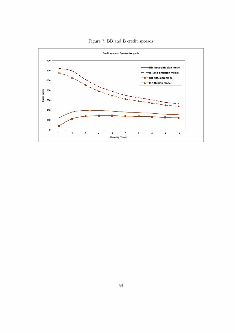
Figure 7: BB and B credit spreads

Credit spreads: Speculative grade

0

200

400

600

800

1000

1200

1400

1 2 3 4 5 6 7 8 9 10

Maturity (Years)

Bas

is p

oint

s

BB jump-diffusion model

B jump-diffusion model

BB diffusion model

B diffusion model

44