
BIS Quarterly Review · Special features in the BIS Quarterly Review ... GBP pound sterling SEK...
116
BIS Quarterly Review December 2017 International banking and financial market developments
Transcript of BIS Quarterly Review · Special features in the BIS Quarterly Review ... GBP pound sterling SEK...

BIS Quarterly ReviewDecember 2017
International bankingand financial market developments

BIS Quarterly Review Monetary and Economic Department
Editorial Committee:
Claudio Borio Stijn Claessens Benjamin Cohen Dietrich Domanski Hyun Song Shin
General queries concerning this commentary should be addressed to Benjamin Cohen (tel +41 61 280 8421, e-mail: [email protected]), queries concerning specific parts to the authors, whose details appear at the head of each section, and queries concerning the statistics to Philip Wooldridge (tel +41 61 280 8006, e-mail: [email protected]).
This publication is available on the BIS website (www.bis.org/publ/qtrpdf/r_qt1712.htm).
© Bank for International Settlements 2017. All rights reserved. Brief excerpts may be reproduced or translated provided the source is stated.
ISSN 1683-0121 (print) ISSN 1683-013X (online)

BIS Quarterly Review, December 2017 iii
BIS Quarterly Review
December 2017
International banking and financial market developments
A paradoxical tightening? .............................................................................................................. 1
Markets in a sweet spot ......................................................................................................... 2
An elusive tightening .............................................................................................................. 6
High valuations: market complacency? ........................................................................ 10
Box : Can CCPs reduce repo market inefficiencies? ................................................ 13
Highlights feature : Risk transfers in international banking .......................................... 15
Box : Interpreting risk transfers in the BIS consolidated banking statistics ...................................................................... 16
The global reallocation of banks’ credit risks ............................................................. 17
The evolution of international risk transfers ............................................................... 20
Special Features
Is there a debt service channel of monetary transmission? .......................................... 23 Boris Hofmann and Gert Peersman
Monetary policy and the debt service ratio ............................................................... 25
Empirical analysis ................................................................................................................... 26
The role of debt ..................................................................................................................... 29
Conclusions ............................................................................................................................. 32
Household debt: recent developments and challenges ................................................. 39 Anna Zabai
How has household debt developed since the GFC? ............................................. 40
Household debt and the economy ................................................................................ 43
Box : Accounting for the increase in the stock of debt: credit demand vs credit supply .................................................................. 44
Conclusions ............................................................................................................................. 51

iv BIS Quarterly Review, December 2017
BIS statistics: Charts ............................................................................................................... A1
Special features in the BIS Quarterly Review ...................................................... B1
List of recent BIS publications ....................................................................................... C1
Notations used in this Review
billion thousand million e estimated lhs, rhs left-hand scale, right-hand scale $ US dollar unless specified otherwise … not available . not applicable – nil or negligible Differences in totals are due to rounding. The term “country” as used in this publication also covers territorial entities that are not states as understood by international law and practice but for which data are separately and independently maintained.

BIS Quarterly Review, December 2017 v
Abbreviations
Currencies
ARS Argentine peso LTL Lithuanian litas
AUD Australian dollar LVL Latvian lats
BGN Bulgarian lev MAD Moroccan dirham
BHD Bahraini dinar MXN Mexican peso
BRL Brazilian real MYR Malaysian ringgit
CAD Canadian dollar NOK Norwegian krone
CHF Swiss franc NZD New Zealand dollar
CLP Chilean peso OTH all other currencies
CNY (RMB) Chinese yuan (renminbi) PEN Peruvian new sol
COP Colombian peso PHP Philippine peso
CZK Czech koruna PLN Polish zloty
DKK Danish krone RON Romanian leu
EEK Estonian kroon RUB Russian rouble
EUR euro SAR Saudi riyal
GBP pound sterling SEK Swedish krona
HKD Hong Kong dollar SGD Singapore dollar
HUF Hungarian forint SKK Slovak koruna
IDR Indonesian rupiah THB Thai baht
ILS Israeli new shekel TRY Turkish lira
INR Indian rupee TWD New Taiwan dollar
JPY Japanese yen USD US dollar
KRW Korean won ZAR South African rand

vi BIS Quarterly Review, December 2017
Countries
AE United Arab Emirates KY Cayman Islands
AR Argentina LB Lebanon
AT Austria LT Lithuania
AU Australia LU Luxembourg
BE Belgium LV Latvia
BG Bulgaria MO Macao SAR
BH Bahrain MT Malta
BM Bermuda MU Mauritius
BR Brazil MX Mexico
CA Canada MY Malaysia
CH Switzerland NG Nigeria
CL Chile NL Netherlands
CN China NO Norway
CO Colombia NZ New Zealand
CR Costa Rica PE Peru
CZ Czech Republic PH Philippines
DE Germany PL Poland
DK Denmark PT Portugal
EA Euro Area RO Romania
EE Estonia RS Serbia
ES Spain RU Russia
FI Finland SA Saudi Arabia
FR France SE Sweden
GB United Kingdom SG Singapore
GR Greece SK Slovakia
HK Hong Kong SAR SL Slovenia
HR Croatia TH Thailand
HU Hungary TR Turkey
ID Indonesia TW Chinese Taipei
IE Ireland UA Ukraine
IL Israel US United States
IN India UY Uruguay
IR Iran VG British Virgin Islands
IS Iceland VN Vietnam
JP Japan ZA South Africa
KR Korea AEs Advanced economies
KW Kuwait EMEs Emerging market economies

BIS Quarterly Review, December 2017 1
A paradoxical tightening?
Markets and the real economy continued their year-long honeymoon during the period under review, which started in early September. Amid further synchronised strength in advanced economies (AEs), mostly solid growth in emerging market economies (EMEs) and, last but not least, a general lack of inflationary pressures, global asset markets added to their year-to-date stellar performance while volatility stayed low. This “Goldilocks” environment easily saw off the impact of two devastating hurricanes in the United States, a number of geopolitical threats, and further steps taken by some of the major central banks towards a gradual removal of monetary accommodation.
Central banks’ actions, on balance, reassured markets. Their varied moves reflected their different positions in the policy cycle. Following its September meeting, the Federal Open Market Committee (FOMC) announced that it would initiate its balance sheet normalisation programme in October, after careful and prolonged communication with markets about strategies and approaches. After 10 years on the sidelines, the Bank of England at its November meeting raised its policy rate by 25 basis points to 0.50%, while keeping the bond purchasing programmes unchanged – which market participants described as a “dovish hike”. In October, the ECB extended the Asset Purchase Programme (APP) at least until September 2018 while halving the monthly purchases, starting in January 2018. The central bank also confirmed that it would stand ready to expand the APP again if macroeconomic conditions deteriorated. The Bank of Japan kept its policy stance unchanged.
Even as the Federal Reserve implemented its gradual removal of monetary accommodation, financial conditions paradoxically eased further in the United States and globally. Only exchange rates visibly priced in the Fed’s relatively tighter stance and outlook, which helped stop and partially reverse the dollar’s year-long slide.
As long-term yields remained extremely low, valuations across asset classes and jurisdictions stayed stretched, though to different degrees. Near-term implied volatility continued to probe new historical lows, while investors and commentators wondered when and how this calm would come to an end. Ultimately, the fate of nearly all asset classes appeared to hinge on the evolution of government bond yields.
2 BIS Quarterly Review, December 2017
Markets in a sweet spot
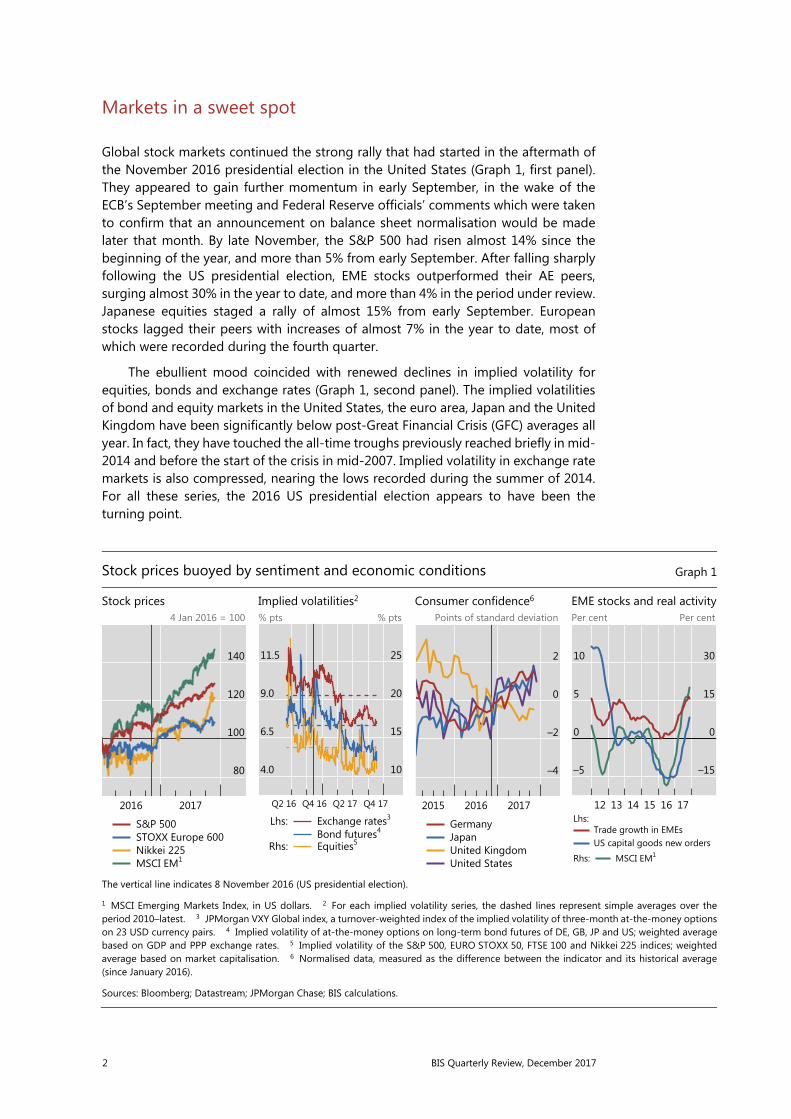
Global stock markets continued the strong rally that had started in the aftermath of the November 2016 presidential election in the United States (Graph 1, first panel). They appeared to gain further momentum in early September, in the wake of the ECB’s September meeting and Federal Reserve officials’ comments which were taken to confirm that an announcement on balance sheet normalisation would be made later that month. By late November, the S&P 500 had risen almost 14% since the beginning of the year, and more than 5% from early September. After falling sharply following the US presidential election, EME stocks outperformed their AE peers, surging almost 30% in the year to date, and more than 4% in the period under review. Japanese equities staged a rally of almost 15% from early September. European stocks lagged their peers with increases of almost 7% in the year to date, most of which were recorded during the fourth quarter.
The ebullient mood coincided with renewed declines in implied volatility for equities, bonds and exchange rates (Graph 1, second panel). The implied volatilities of bond and equity markets in the United States, the euro area, Japan and the United Kingdom have been significantly below post-Great Financial Crisis (GFC) averages all year. In fact, they have touched the all-time troughs previously reached briefly in mid-2014 and before the start of the crisis in mid-2007. Implied volatility in exchange rate markets is also compressed, nearing the lows recorded during the summer of 2014. For all these series, the 2016 US presidential election appears to have been the turning point.
Stock prices buoyed by sentiment and economic conditions Graph 1
Stock prices Implied volatilities2 Consumer confidence6 EME stocks and real activity4 Jan 2016 = 100 % pts % pts Points of standard deviation Per cent Per cent
The vertical line indicates 8 November 2016 (US presidential election).
1 MSCI Emerging Markets Index, in US dollars. 2 For each implied volatility series, the dashed lines represent simple averages over theperiod 2010–latest. 3 JPMorgan VXY Global index, a turnover-weighted index of the implied volatility of three-month at-the-money options on 23 USD currency pairs. 4 Implied volatility of at-the-money options on long-term bond futures of DE, GB, JP and US; weighted average based on GDP and PPP exchange rates. 5 Implied volatility of the S&P 500, EURO STOXX 50, FTSE 100 and Nikkei 225 indices; weighted average based on market capitalisation. 6 Normalised data, measured as the difference between the indicator and its historical average(since January 2016).
Sources: Bloomberg; Datastream; JPMorgan Chase; BIS calculations.
140
120
100
80
20172016
S&P 500STOXX Europe 600Nikkei 225MSCI EM1
11.5
9.0
6.5
4.0
25
20
15
10
Q4 17Q2 17Q4 16Q2 16
Exchange rates3
Bond futures4Lhs:
Equities5Rhs:
2
0
–2
–4
201720162015
GermanyJapanUnited KingdomUnited States
10
5
0
–5
30
15
0
–15
171615141312
Trade growth in EMEsUS capital goods new orders
Lhs:
MSCI EM1 Rhs:

BIS Quarterly Review, December 2017 3
This remarkable performance was once again underpinned by strong economic data. Consumer confidence reached new highs in Germany, Japan and the United States, and stabilised in the United Kingdom (Graph 1, third panel). Growth continued to match or surpass expectations in both AEs and EMEs, and was broad-based. Consumption was strong, and capital expenditure picked up. A revival in trade contributed to the rebound in EME stock markets that had been under way since mid-2016 (Graph 1, fourth panel). Labour markets strengthened further in AEs, helped by the sustained expansion in both manufacturing and services (Graph 2, left-hand panel). Manufacturing activity was also solid, if not as buoyant, in EMEs.
Despite stronger activity, inflationary pressures remained remarkably subdued in most AEs. Inflation rose further above target in the United Kingdom, in the wake of last year’s large currency depreciation, and edged up slightly in Japan while still remaining below target (Graph 2, centre panel). Core inflation continued to be weak in the euro area, even though headline inflation moved closer to target. The change in headline personal consumption expenditure stayed close to 2% in the United States, although the core measure softened as the year went by.
Against this backdrop, the Federal Reserve decided at its September meeting to start implementing in October the balance sheet normalisation plan it had announced in June. As a result, futures markets pointed with near certainty to an additional policy rate hike in December. At the same time, investors appeared to remain sceptical about the Federal Reserve’s resolve to pursue the pace of policy rate increases implied by the median of FOMC members’ “dot plot” forecasts. That said, the gap between those forecasts and market expectations narrowed (Graph 2, right-hand panel).
Solid growth and moderate inflation herald further tightening in the US Graph 2
Manufacturing and services PMIs1 Headline and core inflation4 Dot plot and market expectations5
Diffusion index Per cent Per cent
1 Purchasing managers’ indices. A value of 50 indicates that the number of firms reporting business expansion and contraction is equal; avalue above 50 indicates expansion of economic activity. Weighted average based on GDP and PPP exchange rates of the economies listed. 2 EA, GB, JP and US. 3 AR, BR, CL, CN, CZ, HK, HU, ID, IN, KR, MX, MY, PE, PL, RU, SG, TH, TR and ZA. 4 Based on CPI indices; for US, based on personal consumption expenditure. 5 For market expectations, fed funds 30-day futures implied rate; for 2017, December 2017 contract; for 2018, December 2018 contract; for 2019, December 2019 contract; for 2020, August 2020 contract. 6 Economic projections of US Federal Reserve Board members and US Federal Reserve Bank presidents.
Sources: Bloomberg; Datastream; national data; BIS calculations.
54
52
50
48201720162015
Manufacturing Services
AEs:2
EMEs:3
2
1
0
–120172016
United States Japan Euro area United Kingdom
Headline:
Core:
2.5
2.0
1.5
1.02020201920182017
Median of the Fed dot plot (20 Sep 17)6
1 Sep 201714 Nov 2017
Fed funds futures:
4 BIS Quarterly Review, December 2017
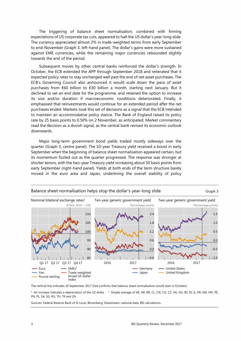
The triggering of balance sheet normalisation, combined with firming expectations of US corporate tax cuts, appeared to halt the US dollar’s year-long slide. The currency appreciated almost 2% in trade-weighted terms from early September to end-November (Graph 3, left-hand panel). The dollar’s gains were more sustained against EME currencies, while the remaining major currencies rebounded slightly towards the end of the period.
Subsequent moves by other central banks reinforced the dollar’s strength. In October, the ECB extended the APP through September 2018 and reiterated that it expected policy rates to stay unchanged well past the end of net asset purchases. The ECB’s Governing Council also announced it would scale down the pace of asset purchases from €60 billion to €30 billion a month, starting next January. But it declined to set an end date for the programme, and retained the option to increase its size and/or duration if macroeconomic conditions deteriorated. Finally, it emphasised that reinvestments would continue for an extended period after the net purchases ended. Markets took this set of decisions as a signal that the ECB intended to maintain an accommodative policy stance. The Bank of England raised its policy rate by 25 basis points to 0.50% on 2 November, as anticipated. Market commentary read the decision as a dovish signal, as the central bank revised its economic outlook downwards.
Major long-term government bond yields traded mostly sideways over the quarter (Graph 3, centre panel). The 10-year Treasury yield received a boost in early September when the beginning of balance sheet normalisation appeared certain, but its momentum fizzled out as the quarter progressed. The response was stronger at shorter tenors, with the two-year Treasury yield increasing about 50 basis points from early September (right-hand panel). Yields at both ends of the term structure barely moved in the euro area and Japan, underlining the overall stability of policy
Balance sheet normalisation helps stop the dollar’s year-long slide Graph 3
Nominal bilateral exchange rates1 Ten-year generic government yield Two-year generic government yield 8 Nov 2016 = 100 Percentage points Percentage points
The vertical line indicates 20 September 2017 (Fed confirms that balance sheet normalisation would start in October).
1 An increase indicates a depreciation of the US dollar. 2 Simple average of AE, AR, BR, CL, CN, CO, CZ, HK, HU, IN, ID, IL, KR, MX, MY, PE,PH, PL, SA, SG, RU, TH, TR and ZA.
Sources: Federal Reserve Bank of St Louis; Bloomberg; Datastream; national data; BIS calculations.
110
105
100
95
90
85Q4 17Q3 17Q2 17Q1 17
EuroYenPound sterling
EMEs2
indexbroad US dollar Trade-weighted
2.4
1.8
1.2
0.6
0.0
–0.620172016
GermanyJapan
1.5
1.0
0.5
0.0
–0.5
–1.020172016
United StatesUnited Kingdom

BIS Quarterly Review, December 2017 5
expectations. Only UK gilt yields shifted significantly upwards in late September, with term spreads staying roughly unchanged as short and long yields moved in lockstep.
Corporate credit spreads continued to narrow, reinforcing the bullish message of equity markets. European high-yield corporate spreads widened the discount over comparable US spreads, helped by mid-November jitters in US high-yield. Before that, the US high-yield market had been plumbing spreads in the low 300s, a level breached only in the run-up to the 1998 Long-Term Capital Management crisis and again almost 10 years later just before the outbreak of the GFC. On the other side of the Atlantic, European high-yield spreads had been lower only occasionally during the period prior to 2007 (Graph 4, left-hand panel). The compression in investment grade spreads was less sharp but equally steady.
Sovereign spreads in EMEs (Graph 4, centre panel) had also been narrowing further until they were buffeted by the same anxieties that affected the US high-yield sector late in the period. Nevertheless, sovereign credit default swap (CDS) spreads were the lowest since the end of the GFC. The resilience in sovereign spreads and strength in equity markets have been buttressed throughout 2017 by sustained capital inflows (Graph 4, right-hand panel).
Overall, global financial conditions paradoxically eased despite the persistent, if cautious, Fed tightening. Term spreads flattened in the US Treasury market, while other asset markets in the United States and elsewhere were buoyant. We explore the potential reasons for this pattern in the next section.
Spreads continue to decline in high-yield credit markets and EME sovereigns Graph 4
Corporate credit1 EME sovereign credit spreads Flows into EME portfolio funds5 Basis points Basis points USD bn
The dashed lines represent simple averages over the period June 2005–June 2007.
1 Option-adjusted spreads over government bonds. For Europe, euro-denominated corporate debt issued in euro domestic and eurobond markets. 2 JPMorgan EMBI Global index, stripped spread. 3 Emerging market CDX.EM index, five-year on-the-run CDS mid-spread. 4 JPMorgan GBI EM indices; spread over seven-year US Treasury securities 5 Monthly sums of weekly data across major EMEs up to 30 October 2017. Data cover net portfolio flows (adjusted for exchange rate changes) to dedicated funds for individual EMEs and to EMEfunds with country/regional decomposition.
Sources: Bank of America Merrill Lynch; EPFR; JPMorgan Chase; BIS calculations.
1,000
800
600
400
200
01716151413121110
United States Europe
High-yield:
Investment grade:
600
500
400
300
200
1001716151413121110
EMBI Global2
EME CDS3Local currencysovereign spread4
20
10
0
–10
–20
–30201720162015
Bond Equity

6 BIS Quarterly Review, December 2017
An elusive tightening
Financial conditions have conspicuously eased in US markets over the last 12 months, despite the Federal Reserve’s gradual removal of monetary accommodation. After raising the federal funds rate target range for the first time in almost 10 years in December 2015, the FOMC has taken several further steps in that direction. Since last December, it has raised the target range another three times, amounting to 75 basis points. Finally in October, it started the process of trimming its $4.5 trillion balance sheet, in a move for which it had been preparing financial markets at least since its March meeting.
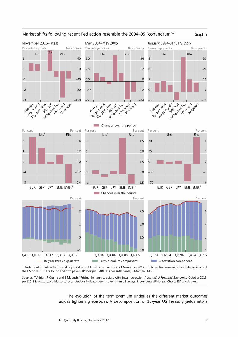
Yet investors essentially shrugged off these moves. Two-year US Treasury yields have indeed risen by more than 60 basis points since December 2016, but the yield on the 10-year Treasury note has traded sideways (Graph 5, first panel).1 Moreover, the S&P 500 has surged over 18% since last December, and corporate credit spreads have actually narrowed, in some cases significantly. Overall, the Chicago Fed’s National Financial Conditions Index (NFCI) trended down to a 24-year trough, in line with several other gauges of financial conditions.
In many respects, the current tightening cycle has so far been reminiscent of its mid-2000s counterpart. During the first year of that cycle, stock markets rose, while long-term Treasury yields and credit spreads dropped in the face of slightly more forceful Fed action (Graph 5, second panel). That said, the broad NFCI did see at least a small tightening then. At the time, Federal Reserve Chair Alan Greenspan had characterised the fall in long-term yields as a “conundrum”.
The experience of these two episodes contrasts markedly with previous tightening cycles. In 1994, for example, the Fed’s actions triggered sharply higher long-term yields, moderate stock market losses, wider credit spreads and a corresponding surge in the NFCI, pointing to a significant tightening of financial conditions (Graph 5, third panel).
The current market response in EMEs has also been more similar to the mid-2000s episode than to that of 1994. As the Fed removed accommodation this time round, financial conditions remained calm in EMEs. From December 2016, sovereign EME spreads (as measured here by the EMBI index) narrowed and EME currencies, on balance, appreciated moderately vis-à-vis the US dollar (Graph 5, fourth panel). Similar patterns had appeared in the first year of the mid-2000s tightening (fifth panel). In contrast, in 1994 the EMBI spread had widened by almost 800 basis points on the back of massive EME currency depreciation (sixth panel).
In all three cases, the dollar depreciated against major AE currencies, reflecting developments in the United States relative to those in other AEs. In the most recent episode, the dollar weakened for much of 2017 as economic prospects brightened in other regions (especially the euro area), recouping a portion of its previous losses in the past few weeks.
1 In fact, after the Fed’s December hike and during most of 2017, the 10-year Treasury yield had been
slowly drawing away from the level reached after the post-US election jump, reflecting in part the fading expectations of fiscal stimulus. The response to the anticipated start of the balance sheet run-off somewhat reversed that fall.
BIS Quarterly Review, December 2017 7
The evolution of the term premium underlies the different market outcomes across tightening episodes. A decomposition of 10-year US Treasury yields into a
Market shifts following recent Fed action resemble the 2004–05 “conundrum”1 Graph 5
November 2016–latest May 2004–May 2005 January 1994–January 1995 Percentage points Basis points Percentage points Basis points Percentage points Basis points
Per cent Per cent Per cent Per cent Per cent Per cent
Per cent Per cent Per cent
1 Each monthly date refers to end of period except latest, which refers to 21 November 2017. 2 A positive value indicates a depreciation of the US dollar. 3 For fourth and fifth panels, JP Morgan EMBI Plus; for sixth panel, JPMorgan EMBI.
Sources: T Adrian, R Crump and E Moench, “Pricing the term structure with linear regressions”, Journal of Financial Economics, October 2013, pp 110–38; www.newyorkfed.org/research/data_indicators/term_premia.html; Barclays; Bloomberg; JPMorgan Chase; BIS calculations.
1
0
–1
–2
–3
40
0
–40
–80
–120
Fed ra
te
2y govt
yield
10y g
ovt yie
ldS&
P 500
Chicag
o Fed FC
IHY s
pread
IG sp
read
18.2Lhs Rhs5.0
2.5
0.0
–2.5
–5.0
24
12
0
–12
–24
Fed ra
te
2y govt
yield
10y g
ovt yie
ldS&
P 500
Chicag
o Fed FC
IHY s
pread
IG sp
read
Lhs Rhs
Changes over the period
9
6
3
0
–3
30
20
10
0
–10
Fed ra
te2y
govt yie
ld
10y g
ovt yie
ldS&
P 500
Chicag
o Fed FC
IHY s
pread
IG sp
read
Lhs Rhs
8
4
0
–4
–8
0.4
0.2
0.0
–0.2
–0.4EUR GBP JPY EME EMBI3
Lhs2 Rhs
9
6
3
0
–3
4.5
3.0
1.5
0.0
–1.5EUR GBP JPY EME EMBI3
Lhs2 Rhs
Changes over the period
70
35
0
–35
–70
6
3
0
–3
–6EUR GBP JPY EME EMBI3
Lhs2 Rhs
2
1
0
–1Q4 17Q3 17Q2 17Q1 17Q4 16
10-year zero coupon rate
4.5
3.0
1.5
0.0Q2 05Q1 05Q4 04Q3 04
Term premium component
6
4
2
0Q1 95Q4 94Q3 94Q2 94Q1 94
Expectation component

8 BIS Quarterly Review, December 2017
future rate expectations component and a term premium suggests that declining term premia drove long-term rates lower both now and during the mid-2000s “conundrum” episode. In both cases, the drop in estimated term premia more than offset the upward revision in expectations about the future path of short-term interest rates (Graph 5, seventh and eighth panels). In contrast, in 1994 the term premium initially increased very swiftly before stabilising and gradually declining later in the year. Nevertheless, the rising rate expectations component predominated (ninth panel). The recent decline in term premia is even more puzzling than in 2005, as the current balance sheet run-off process is specifically aimed at decompressing term premia that were squeezed by the large-scale asset purchases (LSAPs).
The difference between the last two episodes and that of 1994 reflects shifts towards greater gradualism and predictability in the Fed’s tightening strategies. The Fed’s moves in 1994 were steep and less thoroughly communicated to markets. By contrast, gradualism and predictability have characterised the current tightening cycle, with respect to both the policy rate and balance sheet adjustment.
Since December 2016, on average, market participants have been expecting policy rates to rise 40 basis points over the subsequent 12 months (Graph 6, yellow bars in the left-hand panel). While the mid-2000s hiking cycle also featured gradual expectations for rate increases, the 1994 tightening was rather aggressive. On average, the market expected the Fed to raise interest rates at a pace of 100 basis points a year starting in 2004 and 160 basis points in 1994.
Gradualism also defined the programme announced in June for the balance sheet run-off. The planned reduction in Treasury securities holdings is less than $18 billion a month on average till the end of 2018. The pace at which holdings will
Market reaction shaped by gradualism, predictability and policy divergence Graph 6
Shift in expectations1 Central bank total assets Foreign holdings of US long-term securities
Local currency trn Local currency bn % of total outstanding
1 Periods are November 2016–latest, May 2004–May 2005 and January 1994–January 1995, respectively. 2 November 2017; for Margin debt per share, September 2017. 3 Based on eurodollar futures. 4 Average absolute value of the change in the overnight index swap (OIS) rate on meeting dates; based on one-month OIS rate. For 1994–95, one-month Libor rate with adjustment when the OIS rate is not available.
Sources: Federal Reserve Bank of Philadelphia; US Department of the Treasury; Bloomberg; Datastream; SIFMA; national data; BIS calculations.
6
3
0
–3
–62016–latest2 2004–05 1994–95
Average expected pace of tightening (%)3
Average monetary policy shock (bp)4
Change in MOVE Index (scaled by 10)Change in margin debt per share
500
400
300
200
100
4,000
3,000
2,000
1,000
0
171513110907
JapanLhs:
United StatesEuro areaUnited Kingdom
Rhs:
50
45
40
35
30
1717Q2Q1161514131211
TreasuryCorporate debtFederal agency securities

BIS Quarterly Review, December 2017 9
fall is thus likely to be substantially slower than the pace of net Treasury purchases during the LSAP programmes, which ranged from $45 billion to $75 billion a month (Graph 7, left-hand panel). Investors also expected that the resulting increase in duration supplied to the private sector would be modest, at least initially. Some market participants have estimated that the instruments issued by the Treasury to offset the Fed’s reduced reinvestments would have shorter maturities than those that the LSAPs had originally taken out of the market (centre panel).2 In addition, there is a growing consensus among market participants that the Fed’s ultimate balance sheet target size will be much larger than before the GFC. For instance, primary dealers surveyed in June by the Federal Reserve Bank of New York forecasted a balance sheet size of around 15% of GDP as of 2025, compared with the 6% prevailing pre-crisis (right-hand panel).3
In addition to being perceived as gradual, policy decisions in the current cycle were well anticipated. Little or no additional market information was transmitted by the actual policy rate decisions. Measured by the absolute value of daily change in short-term interest rates on policy rate decision days, the surprise was less than 1 basis point on average (Graph 6, red bars in the left-hand panel). Consistent with this, uncertainty about future interest rates, as measured by the MOVE index, was well contained and actually decreased during the course of tightening (blue bars in the left-hand panel). The balance sheet policy was also carefully and extensively communicated. For example, before the Fed announced the effective beginning of the normalisation process at the September 2017 FOMC meeting, 87% of primary
2 The Treasury’s recent announcement that it would keep the size of its auctions of notes and bonds
unchanged up to the end of the first quarter of 2018 appeared to validate such expectations. To compensate for the lost funding from the Fed’s diminished rollover, the Treasury would change the auction sizes of bills and/or cash management bills, which have maturities of up to one year.
3 The forecasted size is conditional on not hitting the zero lower bound (ZLB) again at any point between now and the end of 2025. Given the non-negligible chance of moving back to the ZLB, as perceived by the primary dealers, the unconditional forecasted size is likely to be even larger.
Fed’s balance sheet reduction expected to be gradual Graph 7
Pace of Treasuries purchased during QEs1
Average maturity of Treasuries purchased during QEs3
Fed’s balance sheet
USD bn/month Years Total assets, % of GDP
1 The horizontal line indicates USD 18 billion/month, the average cap of reduction in Treasury holdings between October 2017 and December 2018. The actual reduction is likely to be smaller. 2 Before tapering. 3 The horizontal line indicates five years, the average maturity of additional Treasury issuance estimated by some market participants. 4 Projection based on responses to the Federal Reserve Bank of New York’s Survey of Primary Dealers in June 2017.
Sources: Bloomberg; Datastream; national data; BIS calculations.
80
60
40
20
0QE1 QE2 QE32
12
9
6
3
0QE1 QE2 QE32
16
12
8
4
02000–07 2008–latest 20254

10 BIS Quarterly Review, December 2017
dealers surveyed in September by the New York Fed had already anticipated the announcement.
While rate hikes in 2004 featured similar predictability, the Fed took market participants by surprise in 1994. In the 2004 episode, short-term interest rates moved only around 1 basis point on average on days when the Fed raised the interest rate. The MOVE index declined accordingly. In comparison, short-term interest rates moved by more than 8 basis points on decision days; and the MOVE index rose further as the Fed proceeded with tightening in 1994.
Gradualism and predictability may have contributed to the easing of financial conditions. In the absence of imminent inflationary pressures, such as those prevailing in 1994, in the two more recent episodes the Fed’s gradual approach may have supported investors’ beliefs that the central bank would not risk impairing growth and damaging valuations. That may have compressed risk premia by reducing perceived downside risks. Moreover, research has investigated the various ways in which predictable central bank actions, by removing uncertainty about the future, can encourage leverage and risk-taking.4 Indeed, while investors cut back on the margin debt supporting their equity positions in 1994, and stayed put in 2004, margin debt increased significantly over the last year (Graph 6, purple bars in the left-hand panel).
The relatively accommodative stance of other major central banks may also have supported easier financial conditions in the current cycle. Central bank balance sheets have continued to expand while yields and term premia have remained low in most of the major AEs (Graph 6, centre panel). As a result, despite the Fed’s move towards tightening, the global search for yield has supported buoyant asset prices in the United States. For instance, the growth in the share of US long-term securities held by foreigners, notably corporate debt and federal agency securities, increased in the second quarter of 2017, after a respite earlier in the year (right-hand panel).
High valuations: market complacency?
Tentative moves towards monetary policy normalisation have revived long-standing concerns about asset valuations. Market commentary has increasingly focused on the degree of asset price inflation that unconventional monetary policies may have instilled in different asset classes. Stock market valuations have come under particularly close scrutiny. As the mid-November sell-off illustrated, the spreads on corporate high-yield and sovereign EME bonds have also become more vulnerable to sudden swings in market sentiment. At the root of these uncertainties are questions about how the compression of term premia in core sovereign bond markets may affect other asset valuations. There is also significant uncertainty about the levels those yields will reach once monetary policies are normalised in the core jurisdictions.
According to traditional valuation gauges that take a long-term view, some stock markets did look frothy. At its recent levels in excess of 30, the cyclically adjusted price/earnings ratio (CAPE) of the US stock market exceeded its post-1982 average by almost 25%, comfortably sitting in the highest quartile of the distribution (Graph 8,
4 See C Borio and H Zhu, “Capital regulation, risk-taking and monetary policy: a missing link in the
transmission mechanism”, Journal of Financial Stability, vol 8, issue 4, December 2012, pp 236–51; and V Bruno and H S Shin, “Cross-border banking and global liquidity”, Review of Economic Studies, vol 82, April 2015, pp 535–64.

BIS Quarterly Review, December 2017 11
top left-hand panel). Admittedly, this is still short of the extraordinary peak of 45 reached during the dotcom bubble of the late 1990s. But it is almost twice the long-term average computed over the period 1881–2017. While the available series do not stretch as far back for European and UK equities, their CAPEs were at their post-1982 averages. Meanwhile, the CAPE for Japanese equities was less than 50% its available long-term average. Price/dividend ratios conveyed a similar message.
At the same time, dividends per share of US equities have been growing at a much faster rate since the GFC, giving rise to questions about long-term sustainability (Graph 8, red line in the top right-hand panel). This is because the faster growth was supported in part by a significant shift in corporates’ dividend policy. The share of net income paid out in dividends has increased by more than half over the last five years (blue line in the top right-hand panel). The dividend payout ratio is back to the relatively high levels observed in the 1970s, and thus may be approaching an upper
Stretched multiples in stock markets Graph 8
Equity valuation ratios1 S&P 500 multiples Ratio Ratio USD/share Ratio
S&P 500 share buybacks Listed corporate profits4 USD bn Net income/GDP
1 For cyclically adjusted price/earnings (CAPE) ratio, 1982–2017. For price/dividend: for US, December 1970–latest; for DE, May 1997–latest; for JP, May 1993–latest; for GB, May 1993–latest. 2 For each country/region, the CAPE ratio is calculated as the inflation-adjusted MSCI equity price index (in local currency) divided by the 10-year moving average of inflation-adjusted reported earnings. 3 European advanced economies included in the MSCI Europe index. 4 Net income of listed companies; based on Datastream US equity index.
Sources: Barclays; Bloomberg; Datastream; national data; BIS calculations.
80
60
40
20
0
160
120
80
40
0US EU3 JP GB US DE JP GB
Maximum75th percentile50th percentile25th percentileMinimum
Cyclically adjusted P/E (lhs)2 Price/dividend (rhs)
LatestAverage1881–2017 average
44
33
22
11
0
68
56
44
32
2017120702979287827772
Dividend per share (lhs)Dividend/earnings ratio (rhs)
150
100
50
0
171411080502
6
4
2
0
1712070297928782

12 BIS Quarterly Review, December 2017
bound. High dividends per share were also supported by stock repurchases. Except for a short interlude in 2008–09, share repurchases have been very large since the early 2000s (bottom left-hand panel). When and if interest rates begin to rise, corporates may have the incentive to tilt their capital structure back to equity, or at least to reduce stock repurchases, which could raise further questions about stock market valuations.
Moreover, the upward potential for dividend growth may be limited. Listed corporates’ net income has grown rapidly, in fact much more rapidly than US GDP, since the mid-1990s: the ratio of corporate net income to GDP rose from an average of 1.5% in the 1980s to 5.5% by the mid-2000s, and has fluctuated around that level ever since (Graph 8, bottom right-hand panel). If net income continued growing at this more modest pace, in lockstep with nominal GDP, corporations would not be able to continue growing dividends at current rates while keeping payout ratios constant.
Stock market valuations looked far less frothy when compared with bond yields. Over the last 50 years, the real one- and 10-year Treasury yields have fluctuated around the dividend yield (Graph 9, left-hand panel). Having fallen close to 1% prior to the dotcom bust, the dividend yield has been steadily increasing since then, currently fluctuating around 2%. Meanwhile, since the GFC, real Treasury yields have fallen to levels much lower than the dividend yield, and indeed have usually been negative. This comparison would suggest that US stock prices were not particularly expensive when compared with Treasuries.
Investors are sanguine despite compression in fixed income markets Graph 9
Dividend yield and US Treasury real yields
Credit and sovereign spreads1 MOVE and swaption skew
Per cent Basis points Basis points Percentage points
1 1998–latest; for EME local and EME USD, 2002–latest. 2 Corporate spread gap, US minus EA. 3 JPMorgan GBI-EM Index, seven- to 10-year maturity, yield to maturity. 4 JPMorgan EMBI Global, seven- to 10-year maturity, yield to maturity.
Sources: Bank of America Merrill Lynch; Bloomberg; JPMorgan Chase; national data; BIS calculations.
7.5
5.0
2.5
0.0
–2.5
–5.0
–7.517120702979287827772
S&P 500 index dividend yieldOne-yearReal govt yield: Ten-year
550
440
330
220
110
0
2,000
1,600
1,200
800
400
0
US IG
EU IG
Asset s
pread
2US H
YEU
HYEM
E loca
l3EM
E USD
4
Maximum75th percentile50th percentile25th percentileMinimum
Lhs Rhs
Latest
Average
100
80
60
40
20
0
–20171615141312
indexMOVE
+/– 25 bpUSD 3-month/10-year skew:
+/– 100 bp

BIS Quarterly Review, December 2017 13
Can central counterparties (CCPs) reduce repo market inefficiencies? Iñaki Aldasoro, Torsten Ehlers and Egemen Eren
Repo markets have taken on an increasingly important role in global money markets since the Great Financial Crisis as unsecured borrowing has dwindled. But repo markets remain segmented. In the United States, there has been a persistent spread between general collateral financing (GCF) and triparty repo rates. Ultimate borrowers that cannot access the triparty market face higher costs. Money market funds (MMFs) that cannot access the delivery-versus-payment (DvP) or GCF markets to lend cash increase their take-up of the Federal Reserve’s overnight reverse repurchase (ON RRP) facility, which pays a lower rate. Moreover, the retreat of dealers from repo markets at quarter-ends generates spikes in both prices and volumes: both GCF rates and the take-up of repos by MMFs under the ON RRP increase at quarter-ends (Graph A, left-hand panel).
Against this background, an important recent development is a rule change by The Depository Trust & Clearing Corporation (DTCC), approved by the Securities and Exchange Commission in May. This change allows DTCC’s subsidiary, the Fixed Income Clearing Corporation (FICC), to expand the availability of clearing in the repo market to a broader set of institutional investors. Through this rule change, MMFs can provide cash or securities in the DvP markets through a dealer sponsor.
Some MMFs have already started clearing repos through the FICC. The total amount of centrally cleared repos stood at $13 billion at end-October 2017 (Graph A, centre panel). The volumes are still small compared with the total volumes in the triparty market or even compared with other funds belonging to the same fund family. But they have been growing rapidly. Centrally cleared repos made up close to 6% of the total repo volumes of the three fund families that cleared repos through the FICC in October 2017.
Cleared repos replace reverse repos with the Fed Graph A
Recent evolution of repo pricing Centrally cleared repos by MMFs rise4
Reverse repos with the Fed
USD bn Per cent Per cent USD bn USD bn
1 Reverse repo. 2 Bank of New York Mellon Treasury Tri-Party Repo Index (Treasury “TRIP”). 3 DTCC GCF Repo Index (Treasury Weighted Average). 4 For the three major fund families. Other cleared repo volumes are small. 5 Share of FICC repos cleared through a CCP. 6 Includes the funds “Financial Square Government Fund” and “Financial Square Treasury Obligations”. 7 Includes the funds “Federated Government Reserves Fund” and ”Federated Capital Reserves Fund”. 8 Includes the funds “Government & Agency Portfolio”, “Treasury Portfolio”, “Premier U.S. Government Money Portfolio”, “INVESCO Money Market Fund” and “INVESCO V.I. Money MarketFund”. 9 Reverse repos with the Federal Reserve by funds that invest with the FICC (footnotes 5–7). 10 Reverse repos with the Federal Reserve by funds belonging to the same fund families but which do not clear repos with the FICC. 11 Counterfactual reverse repos with the Federal Reserve by funds that trade with the FICC, had they grown their trades with the Fed in the same way as non-CCP funds of the same fund families. Sources: Federal Reserve Bank of St Louis FRED; DTCC; Bank of New York Mellon; Office of Financial Research; BIS calculations.
375
250
125
0
1.05
0.70
0.35
0.00
201720162015
RRP1 total (lhs) Triparty2
GCF3
RRP
Rhs:
6
4
2
0
15
10
5
0
OctSepAugJulJunMayApr2017
CCP share5Lhs: GS6Rhs: Federated7 Invesco8
35
30
25
20
Q3 2017Q1 2017
CCP funds9
Non CCP funds10
CCP funds counterfactual11

14 BIS Quarterly Review, December 2017
Some froth was also present in corporate credit markets even in relation to core sovereign bonds. Credit spreads appeared to be rather compressed, especially in the high-yield space. Looking at the last 20 years of data, both US and European investment grade corporate spreads were below their long-term averages (Graph 9, centre panel). In the high-yield segment, European spreads almost touched their all-time lows, whereas US spreads were only at the door of the lowest quartile of the distribution. The US dollar-euro spread differential, which is itself near its maxima outside stress situations, has contributed to the recent expansion in issuance of euro-denominated paper by US corporates.5
In contrast, EME sovereign bond markets looked to be within their historical average ranges. Spreads in both local currency and the US dollar were relatively closer to their historical averages, going back to the early 2000s (Graph 9, centre panel). Spreads on local currency-denominated government debt are actually above the 15-year average. Compression is more visible in US dollar-denominated issues, with EMBI Global spreads sitting about 65 basis points below the long-term mean, in the second lowest quartile of the distribution. In the past, very low spreads in US high-yield and EME dollar sovereign bond spreads were a harbinger of stress.
In spite of these considerations, bond investors remained sanguine. The MOVE index suggested that US Treasury volatility was expected to be very low, while the flat swaption skew for the 10-year Treasury note denoted a low demand to hedge higher interest rate risks, even on the eve of the inception of the Fed’s balance sheet normalisation (Graph 9, right-hand panel). That may leave investors ill-positioned to face unexpected increases in bond yields.
5 This is one of the factors that appear to underlie the persistent breakdown of covered interest rate
parity. See C Borio, R McCauley, P McGuire and V Sushko, “Covered interest parity lost: understanding the cross-currency basis”, BIS Quarterly Review, September 2016, pp 45–64.
The initial response by the MMFs that clear repos through the FICC suggests that central clearing could
potentially reduce market segmentation. There are already signs of convergence of prices, as centrally cleared repo trades earned up to 12 basis points more than the triparty rate index. Furthermore, funds that cleared trades through the FICC reduced their end-of-quarter take-up of the ON RRP compared with their peer funds (Graph A, right-hand panel). If these funds had instead increased their reverse repos with the Fed at the same rate as their peers, Fed RRPs at end-September 2017 would have been around $35 billion instead of the actual and much lower volume of $21 billion. Source: SEC N-MFP filings.

BIS Quarterly Review, December 2017 15
Risk transfers in international banking1
Credit risk transfers shift a bank’s country exposures from one counterparty country to another. Risk transfer patterns can shed light on how creditor banking systems assess and manage credit risks across counterparty countries. These patterns are closely linked to the business models and international footprint of global banks and corporates. Global banks have taken on more credit risks vis-à-vis some major emerging market economies – in particular in Asia. This points both to the enlarged international footprint of corporates and banks from these countries, and to the willingness of global banks to retain these country exposures on their balance sheets instead of seeking guarantees or hedging them.
International risk transfers shift a bank’s exposure from one counterparty country to another. They include parent and third-party guarantees, credit derivatives (protection purchased) and collateral.2 Risk transfers are therefore conditional claims, which materialise when an immediate borrower cannot service its debts.3
Risk transfers reallocate banks’ exposures from the immediate counterparty country to the country where the ultimate obligor is located. They can be either outward risk transfers, which result in a reduction in banks’ risk exposures to a given counterparty country, or inward risk transfers, which increase them. However, the underlying risk does not disappear, but is merely reallocated, since an outward risk transfer vis-à-vis one country is an inward risk transfer vis-à-vis the country that becomes the ultimate obligor. Claims in the BIS consolidated banking statistics (CBS) are reported on both an immediate counterparty (IC) and an ultimate risk (UR) basis.
1 Starting with this issue of the BIS Quarterly Review the regular chapter on “Highlights of global
financial flows” will be replaced with a short essay on structural or cyclical trends in the global financial system, drawing on the BIS international banking, derivatives and securities statistics. Commentary on quarter-to-quarter changes in the statistics can be found in the statistical releases posted on the BIS website at www.bis.org/statistics/index.htm. Statistical support was provided by Zuzana Filkova. The views expressed in this article are those of the authors and do not necessarily reflect those of the BIS.
2 For examples of how different risk transfers are recorded in the BIS consolidated banking statistics, see the box and “Highlights of the BIS international statistics”, BIS Quarterly Review, March 2011, pp 16–17.
3 See BIS, Potential enhancements to the BIS international banking statistics: report submitted by a Study Group established by the BIS, March 2017. The eligibility criteria for risk transfers within the BIS consolidated banking statistics are similar to those in the Basel Committee on Banking Supervision’s risk mitigants for calculating risk-weighted exposures. The main difference concerns the treatment of collateral, which under Basel Committee standards is deducted from claims.
Iñaki Aldasoro
Torsten Ehlers

16 BIS Quarterly Review, December 2017
Net risk transfers (NRTs), defined as the difference between inward risk transfers and outward risk transfers, introduce a wedge between a reporting country’s banking system claims on an IC and a UR basis (box).
This feature assesses the size, scope and evolution of international risk transfers. The use of risk transfers by BIS reporting banks is mainly determined by the riskiness of counterparty countries. Therefore, risk transfers can shed light on how creditor banking systems assess and manage credit risks across counterparty countries. This is closely linked to the business models and international footprint of global banks and corporates.
There have been a number of important structural shifts in risk transfers in the past decade. To be sure, some patterns have remained unchanged. Banks have continued to transfer credit risks out of international financial centres and riskier countries, and into advanced economies.4 Even so, there has been a significant change in patterns vis-à-vis emerging market economies (EMEs), as banks have increased credit exposures to emerging Asia. This has been driven in part by the
4 See Committee on the Global Financial System, Improving the BIS international banking statistics,
CGFS Papers, no 47, November 2012; and S Avdjiev, P McGuire and P Wooldridge, “Enhanced data to analyse international banking”, BIS Quarterly Review, September 2015, pp 53–68.
Interpreting risk transfers in the BIS consolidated banking statistics
The BIS consolidated banking statistics (CBS) record net risk transfers, as well as gross inward and outward risk transfers. Inward risk transfers increase the credit risk exposures vis-à-vis a given counterparty country, whereas outward risk transfers reduce them, by passing them on to another counterparty country. Net risk transfers (NRTs) are defined as inward risk transfers minus outward risk transfers.
There are three types of eligible risk transfers for a creditor bank: parent and third-party guarantees, credit derivatives (protection purchased) and collateral transfers (see examples A–D in Graph A). A major share of risk transfers occurs either between internationally active banks or between a bank and a non-bank financial institution. For instance, in a collateralised borrowing transaction between banks, such as a repurchase agreement (example B), a creditor bank transacts with another bank to transfer the credit risk exposure vis-à-vis the counterparty country to the country of the collateral issuer (eg the United States in the case of US Treasury collateral).
Internationally active banks and other financial institutions also commonly buy and issue credit derivatives, such as credit default swaps (CDS, example A). If a creditor bank purchases a CDS from an entity located in country A to hedge an exposure to country B, the bank records an inward risk transfer vis-à-vis country A and an outward risk transfer vis-à-vis country B, both equal to the notional amount of protection purchased. Analogously, explicit guarantees transfer risk to the guarantor (example C). A special case in the CBS are credit exposures vis-à-vis foreign branches of banks. Consistent with standards set out by the Basel Committee on Banking Supervision, claims on bank branches are assumed to be guaranteed by the headquarters, even if no explicit guarantees are in place. In all other cases, guarantees need to be explicit.
In all of the above examples, credit exposures vis-à-vis a foreign counterparty may also be transferred to another institution in the home country (home country risk transfer). Home country risk transfers are typically driven by globally active firms in the home country (example D). Another example would be export or foreign direct investment credit guarantees provided by the government of the home country. Risk transfers vis-à-vis the home country therefore provide a measure of the share of foreign credit exposures that are ultimately against counterparties in the home country of the creditor bank. As risk transfers merely reallocate risks, but do not reduce or increase overall credit risk from the point of view of the creditor country, net risk transfers across all counterparty countries sum to zero. Risk transfers vis-à-vis foreign countries and home country risk transfers therefore mirror each other.

BIS Quarterly Review, December 2017 17
expanding international footprint of EME corporates and banks. It may also reflect creditor banks’ growing willingness to retain risk exposures to these countries as their economic strength and creditworthiness have improved.
The global reallocation of banks’ credit risks
The spectrum of banks’ credit risk transfers across a wide range of counterparty countries illustrates how differences in global banks’ business models, the international footprint of corporates and the riskiness of counterparty countries drive global reallocations of banks’ credit risks.
Types of eligible risk transfers Graph A
Example Reporting country
Counterparty country
IC claims (1)
Inward risk transfers (2)
Outward risk transfers (3)
UR claims = (1) + (2) – (3)
A, B and C France Japan $1bn 0 $1bn 0
France US 0 $1bn 0 $1bn
D France Japan $1bn 0 $1bn 0
France France 0 $1bn 0 $1bn
The treatment of collateral, however, varies across reporting countries. Risk transfers are likely to be underreported, as some countries do not report risk transfers related to repos or exchanges of collateral. On the other hand, inward and outward risk transfers may overstate cross-border transfers because some reporting countries include risk transfers between counterparties within the same country. The sum of risk transfers vis-à-vis foreign countries and the home country can deviate from zero due to reporting errors and omissions.
Bank in Japan French bank Cash $1bn
US Treasuries collateral
worth $1bn
Example B: Collateral transfer
Bank in Japan French bank Loan $1bn
Bank in the US
CDS on bank in Japan with notional $1bn
$10m payment
Example A: Purchase of credit protection
French firm’s subsidiary in
Japan French bank
French firm’s headquarters
in France
Loan $1bn
Guarantee for the loan of $1bn
Example D: Guarantee - home country risk transfer
US firm in Japan French bank Loan $1bn
US government
Guarantee for the loan of $1bn
Example C: Guarantee

18 BIS Quarterly Review, December 2017
Banks transfer a large amount of credit risk out of financial centres, such as the United Kingdom or the Cayman Islands. This is reflected in large negative NRTs vis-à-vis these jurisdictions (Graph 1, grey bars). Large banks from advanced economies as well as EMEs maintain branches in European and offshore financial centres. Guarantees from the parent bank5 transfer the risk out of the financial centre where the branch is located and into the home country of the parent bank. Analogously, risk is transferred out of an offshore financial centre if a corporate issues bonds through a financial holding company domiciled there, and the parent company guarantees the bonds.6
Risk transfers out of financial centres are the largest negative NRTs globally. For instance, at end-June 2017 credit risks with a notional value of close to $200 billion (16% of foreign claims on an IC basis) were transferred out of the Cayman Islands on a net basis. For European financial centres (including Belgium, Luxembourg, the Netherlands, Switzerland and the United Kingdom) NRTs amounted to around –$220 billion.
At the other end of the spectrum are those advanced and emerging market economies where international banking business primarily reflects the activity of locally headquartered banks, such as China, Germany, Japan, Korea or the United States. To some extent, this is a mirror image of risk transfers out of financial centres: one driver of the large positive NRTs are advanced economy parent banks’
5 Claims on branches are assumed to be guaranteed by the parents, generating outward (negative)
risk transfers vis-à-vis the country where the branch is located. See also the box.
6 For example, consider a corporate from an EME that issues bonds in an offshore financial centre. If the bonds are held by an advanced economy reporting bank, this will be reflected in an IC claim of the advanced economy’s banking system on the offshore centre. However, provided there is a parent guarantee, the ultimate obligor is the EME in which the corporate is headquartered: on a UR basis the claim is vis-à-vis the EME and not the offshore centre.
Risk transfers vis-à-vis selected foreign counterparty countries1
At end-June 2017 Graph 1
Per cent USD bn
1 Inward and outward risk transfers do not necessarily sum up to net risk transfers as not all reporting countries provide data for inward and outward risk transfers. 2 FC = European financial centres: BE, CH, GB, LU and NL. 3 OF = offshore financial centres excluding HK, KY, SG. The amount of net risk transfers for all offshore financial centres equals –$507 billion. 4 ME = emerging Africa and Middle East. 5 CE = emerging Europe. 6 LA = emerging Latin America and Caribbean. 7 AS = emerging Asia and Pacific. 8 AE = advanced economies excluding European financial centres.
Sources: BIS consolidated banking statistics; authors’ calculations.
10
0
–10
–20
–30
100
0
–100
–200
–300FC2 OF3 LU ME4 CE5 LA6 SA PL HU ZA RU MY BR KR DE CN
KY HK GB NL SG MX TR TH AR CL CH IN JP US AS7 AE8
Inward risk transfersShare in foreign claims (lhs): Outward risk transfers Net risk transfers Rhs:

BIS Quarterly Review, December 2017 19
guarantees to their branches located in financial centres. Further, these economies are home to large globally active non-financial firms. If bank claims on the foreign operations of these firms are guaranteed by the parent or third parties in the home country (eg through government export or investment guarantees), banks’ credit risks are transferred back into those countries. Indeed, home country risk transfers are also significant for the large economies mentioned above (Table 1). For some major economies, such as the US or Germany, a relevant share of positive (inward) risk transfers results from the use of their government securities as collateral in secured borrowing transactions (Graph A, example B).
The other key determinant of banks’ international risk transfers is the perceived riskiness of counterparty countries. For instance, NRTs vis-à-vis countries in the Middle East and Africa, as well as most countries in Latin America, are negative (Graph 1). At the same time, risks are transferred into advanced economies on a global level. The ratio of outward risk transfers to foreign claims on an IC basis (a kind of “hedge ratio”) best captures the degree to which global banks hedge risks vis-à-vis certain counterparty countries (Graph 1, blue triangles). Whether these hedges are effective, however, depends on the probability of double default of the borrower and the ultimate obligor.
Risk transfers into and out of BIS reporting banking systemsAt end-June 2017, in billions of US dollars
Table 1Banking system Vis-à-vis all countries Vis-à-vis foreign countries Vis-à-vis home country
Claims1 NRTs2 Claims1 NRTs2 Claims1 NRTs2
Austria 703 0 341 –4 362 4
Belgium 530 0 215 –1 314 1
Canada 3,440 1 1,494 1 1,946 0
Chile 180 0 12 0 169 0
Chinese Taipei 1,446 0 305 –23 1,141 23
France 6,955 1 2,832 –9 4,123 10
Germany 7,406 0 2,256 –305 5,151 305
Greece 334 0 84 0 250 0
Japan 18,864 0 3,992 –158 14,872 158
Korea 1,865 0 168 –7 1,697 7
Singapore 824 0 466 12 359 –12
Spain 3,323 0 1,602 –12 1,721 12
Sweden 1,570 0 847 –9 723 9
Switzerland 2,837 0 1,425 –54 1,411 54
United Kingdom 5,709 0 3,172 25 2,537 –25
United States 13,962 0 3,165 –30 10,797 30 1 Claims on an immediate counterparty basis. 2 Net risk transfers: inward minus outward risk transfers.
Sources: BIS consolidated banking statistics; authors’ calculations.

20 BIS Quarterly Review, December 2017
The evolution of international risk transfers
While NRTs vis-à-vis advanced economies and financial centres have been largely stable since the Great Financial Crisis (Graph 2, left-hand panel),7 banks’ risk transfers vis-à-vis EMEs – in particular emerging Asia – have changed substantially (right-hand panel). In early 2007, reporting banks transferred around 5.7% of their net exposures out of emerging Asia; by mid-2017, they reported net transfers into the region equalling 6.5% of their foreign IC claims on the region. Underlying the shift in NRTs vis-à-vis emerging Asia is a change in the composition of creditor banking systems. As European banks retreated, banks from Chinese Taipei, Hong Kong SAR, Japan and Singapore increased their exposures to emerging Asia. In Latin America and other emerging market regions, outward risk transfers have continued to exceed inward risk transfers, as reporting banks, in aggregate, choose to offload their exposures vis-à-vis countries in these regions.
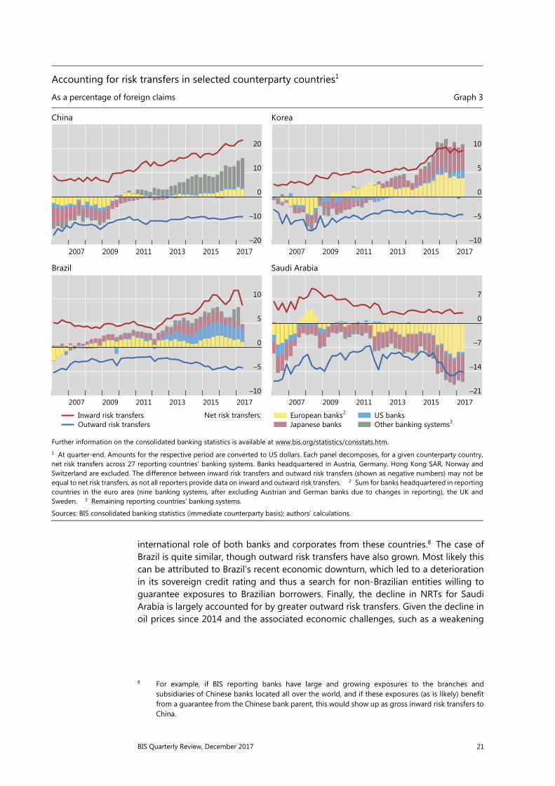
To better understand the drivers of NRTs, Graph 3 decomposes net risk transfers vis-à-vis selected EMEs into the different contributions of BIS reporting banking systems, and plots both outward and inward risk transfers as a percentage of foreign claims on an IC basis.
Different forces have driven these developments in NRTs vis-à-vis EMEs. For countries such as China and Korea, they can be largely explained by the strong rise in inward risk transfers. This probably reflects the increased global footprint and
7 Banks did shift risk out of euro area countries around the time of the European sovereign debt crisis,
but this abated towards the end of 2013.
Evolution of net risk transfers, by counterparty region
As a percentage of foreign claims1 Graph 2
Advanced economies and financial centres Emerging market economies
Further information on the consolidated banking statistics is available at www.bis.org/statistics/consstats.htm. 1 At quarter-end. Amounts for the respective period are reported already converted to US dollars. There are 27 banking systems reportingrisk transfers. German, Norwegian, Swiss and US banks are excluded due to changes in reporting or for confidentiality reasons.
Sources: BIS consolidated banking statistics (immediate counterparty basis); authors’ calculations.
14.0
0.5
–13.0
–26.5
–40.0
5
0
–5
–10
–15201720152013201120092007
Offshore centresLhs: Euro areaUnited KingdomUnited StatesOther AEs
Rhs:
3.4
0.0
–3.4
–6.8
–10.2201720152013201120092007
Emerging Latin America and CaribbeanEmerging Asia and PacificOther EMEs
BIS Quarterly Review, December 2017 21
international role of both banks and corporates from these countries.8 The case of Brazil is quite similar, though outward risk transfers have also grown. Most likely this can be attributed to Brazil’s recent economic downturn, which led to a deterioration in its sovereign credit rating and thus a search for non-Brazilian entities willing to guarantee exposures to Brazilian borrowers. Finally, the decline in NRTs for Saudi Arabia is largely accounted for by greater outward risk transfers. Given the decline in oil prices since 2014 and the associated economic challenges, such as a weakening
8 For example, if BIS reporting banks have large and growing exposures to the branches and
subsidiaries of Chinese banks located all over the world, and if these exposures (as is likely) benefit from a guarantee from the Chinese bank parent, this would show up as gross inward risk transfers to China.
Accounting for risk transfers in selected counterparty countries1
As a percentage of foreign claims Graph 3
China Korea
Brazil Saudi Arabia
Further information on the consolidated banking statistics is available at www.bis.org/statistics/consstats.htm. 1 At quarter-end. Amounts for the respective period are converted to US dollars. Each panel decomposes, for a given counterparty country,net risk transfers across 27 reporting countries’ banking systems. Banks headquartered in Austria, Germany, Hong Kong SAR, Norway and Switzerland are excluded. The difference between inward risk transfers and outward risk transfers (shown as negative numbers) may not be equal to net risk transfers, as not all reporters provide data on inward and outward risk transfers. 2 Sum for banks headquartered in reporting countries in the euro area (nine banking systems, after excluding Austrian and German banks due to changes in reporting), the UK and Sweden. 3 Remaining reporting countries’ banking systems.
Sources: BIS consolidated banking statistics (immediate counterparty basis); authors’ calculations.
20
10
0
–10
–20201720152013201120092007
10
5
0
–5
–10201720152013201120092007
10
5
0
–5
–10201720152013201120092007
Net risk transfers:Inward risk transfersOutward risk transfers
7
0
–7
–14
–21201720152013201120092007
European banks2
Japanese banksUS banksOther banking systems3

22 BIS Quarterly Review, December 2017
of external positions, creditors may have been seeking to lower their risk exposures vis-à-vis oil-exporting countries in the Middle East.9
Graph 4 examines in more detail the relationship between banks’ risk transfers to EMEs and the creditworthiness of the counterparty country. Changes to the riskiness of the counterparty are proxied by changes in the country’s sovereign credit rating. From 2006 to 2016, NRTs as a share of foreign claims on an IC basis tended to increase for major EMEs with improved ratings (Graph 4, left-hand panel). Likewise, outward risk transfers (also as a share of foreign IC claims) decreased vis-à-vis those countries with improved ratings, ie transfers fell as the perceived strength of the country improved (Graph 4, centre panel). The same relationship is apparent when we compare total NRTs vis-à-vis major EMEs with the riskiness of a broad EME portfolio, as measured by a claims-weighted average rating across 22 large EMEs (Graph 4, right-hand panel).
9 See “Highlights of the BIS international statistics”, BIS Quarterly Review, June 2017, pp 5–7. Graph 3
presents data for only Saudi Arabia for illustrative purposes. However, a similar pattern emerges in terms of NRTs for other oil-exporting countries such as Egypt, Oman and the United Arab Emirates.
Risk transfers and rating changes in emerging market economies1 Graph 4
NRTs rise when ratings improve2 ORTs fall when ratings improve3 More NRTs when EMEs are less risky4
1 EMEs = AR, BR, CL, CN, CO, CZ, HU, ID, IN, KR, MX, MY, PH, PL, QA, RU, SA, TH, TR, TW, UA and ZA. There are 27 banking systems reporting risk transfers. Austrian banks are excluded due to reporting changes. Rating is an average of the ratings of Moody’s, Standard & Poor’s and Fitch taken from Bloomberg, transformed to a numerical scale; higher numbers indicate a better rating. Ratings were available from two agencies (Standard & Poor’s and Fitch) for India, and one (Standard & Poor’s) for Chinese Taipei. 2 For each EME: change in the ratio of net risk transfers (NRT) to foreign claims on an immediate counterparty (IC) basis between Q4 2006 and Q4 2016 versus change in country ratingover the same period. 3 For each EME: change in the ratio of outward risk transfers (ORT) to foreign IC claims between Q4 2006 and Q4 2016 versus change in country rating over the same period. 4 For each quarter in the period Q4 2006 to Q4 2016 for the entire group of EMEs:total dollar value of all NRTs versus weighted average rating of EME portfolio. 5 IC foreign claims-weighted average rating of the group ofEMEs.
Sources: Bloomberg; BIS consolidated banking statistics (IC basis); authors’ calculations.
2
0
–2
–43020100–10
Δ ra
ting
Δ NRT/IC
y = – 0.19 + 0.12xR2 = 0.30
2
0
–2
–41050–5–10
Δ ra
ting
Δ ORT/IC
y = 0.06 – 0.26xR2 = 0.34
14.2
13.8
13.4
13.0100500–50–100
Wei
ghte
d ra
ting
EME
port
folio
5
Total NRT (USD bn)
y = 14 + 0.01xR2 = 0.65

BIS Quarterly Review, December 2017 23
Is there a debt service channel of monetary transmission?1
Previous research has explored the impact of private sector debt service ratios (DSRs), ie debt payments relative to income, on medium-term macroeconomic outcomes. This special feature, based on a study of 18 economies, finds that monetary policy shocks, in turn, have a significant impact on DSRs. We show that a monetary tightening leads to a significant and persistent increase in DSRs, with higher effective lending rates on the stock of debt outweighing a decline in the debt-to-income ratio. Moreover, the impact of monetary policy shocks on DSRs, as well as on economic activity, the price level, house prices and credit, turns out to be significantly larger in high-debt economies. These findings point to the existence of a debt service channel of monetary transmission.
JEL classification: E52.
There is growing evidence that high and rising debt is associated with sub-par medium-term growth (Jordà et al (2013), Mian et al (2017), Lombardi et al (2017)). Drehmann et al (2017) find that this effect is mainly attributable to changes in the debt service ratio (DSR), defined as the ratio of total debt payments (principal and interest) to the income of the private non-financial sector.2
Changes in the DSR can have aggregate macroeconomic effects, not only redistributive effects, if debtors and creditors differ in terms of their marginal propensities to consume and invest. Since debtors are typically credit- or liquidity-constrained, they are likely to have greater propensities to consume or invest out of changes in disposable income than creditors (Tobin (1982), Eggertsson and Krugman (2012), Kaplan and Violante (2014), Auclert (2017)). This notion is supported by empirical evidence (eg Mian and Sufi (2014), La Cava et al (2016) and Cloyne et al (2016)). Accordingly, an increase in the aggregate DSR, by transferring income from debtors to creditors, could reduce aggregate output because the decline in spending by debtors is only partially compensated by a rise in spending by creditors.
1 The authors would like to thank Bruno Albuquerque, Claudio Borio, Stijn Claessens, Benjamin Cohen,
Selien De Schryder, Mathias Drehmann, Mikael Juselius and Hyun Song Shin for helpful comments and Matthias Lörch for assistance with the graphs. The views expressed are those of the authors and do not necessarily reflect those of the BIS.
2 Previously, Juselius and Drehmann (2015) have documented a key role for DSRs in driving expenditures. DSRs have also been shown to be a useful short-term early warning indicator for financial distress (Drehmann and Juselius (2012, 2014)).
Boris Hofmann
Gert Peersman

24 BIS Quarterly Review, December 2017
Conversely, a lower DSR could boost economic activity because of the income transfer from creditors to debtors.
These observations suggest that the DSR might also be an important channel in the transmission of monetary policy. Indeed, the extraordinary monetary accommodation provided by the leading central banks in the wake of the Great Financial Crisis (GFC) was in part motivated by a desire to reduce the debt service burdens of households and firms through lower interest rates. And an oft-heard argument in the current debate about the appropriate pace of monetary policy normalisation is that high debt makes the economy more interest rate-sensitive, so that normalisation in highly indebted countries should proceed very cautiously.
Conceptually, however, the impact of monetary policy on the DSR is not clear a priori. In particular, the DSR depends on the debt-to-income ratio of the private sector, as well as on the effective lending rate that has to be paid on the debt. While there is a positive link between changes in the stance of monetary policy and the effective lending rate that is likely to dominate in the short term, the impact on the debt-to-income ratio that kicks in over medium-term horizons typically goes in the opposite direction. Put differently, a policy easing lowers the interest rate that debtors have to pay, but also raises the stock of debt relative to income, and vice versa for a policy tightening. Moreover, the evolution of the policy rate itself, ie the persistence of the policy tightening or easing, also matters for the dynamic response of the DSR to the monetary policy impulse. How monetary policy affects debt service burdens over different horizons is hence ultimately an empirical question.
In this special feature, we explore the transmission of monetary policy through the DSR in the context of an otherwise standard vector autoregression (VAR) for monetary policy analysis. Specifically, extending the approach in Hofmann and Peersman (2017), we analyse the impact of a monetary policy shock (ie a conventional interest rate shock) on the private non-financial sector DSR and its components in a panel of 18 economies over a sample period from the mid-1980s to the onset of the GFC.
There are two main findings. First, a monetary policy tightening triggers a significant and persistent increase in the DSR. Higher policy rates increase effective lending rates, and this effect dominates a fall in debt-to-income ratios, a finding that is consistent with the results of Juselius et al (2017). Second, monetary policy has a stronger impact on DSRs, as well as on economic activity, the price level, house prices and credit, in economies where private sector debt is higher. Although there might be alternative explanations, the stronger effects of monetary policy in high-debt countries may reflect the presence of a debt service channel of monetary transmission. Specifically, a higher debt-to-income ratio mechanically boosts the impact of a change in interest rates on DSRs, and through this channel possibly also on the wider economy.3
3 Recent studies have focused on a possible weakening of monetary transmission when there is a debt
overhang in the private sector as a consequence of the attenuating effects of deleveraging motives. In such situations, borrowers decide to lower expenditures in order to cut their debt burdens and restore their wealth through higher saving (Mian and Sufi (2014)). Giving priority to balance sheet repair over intertemporal expenditure smoothing could then dampen the impact of lower rates on economic activity (eg Koo (2009) and Di Maggio et al (2017)). For example, Alpanda and Zubairy (2017) find for the United States that monetary transmission is weaker in periods of debt overhang, measured as the deviation of debt from its long-term trend. Note that our results suggest that a higher level of debt can strengthen monetary transmission across economies and over time through the DSR, which is not necessarily incompatible with a possibly weaker transmission in periods of large

BIS Quarterly Review, December 2017 25
The remainder of the article is organised as follows. Section 1 discusses the impact of monetary policy on DSRs in general terms. Section 2 presents the empirical analysis, while Section 3 analyses the role of the level of debt in the transmission of monetary policy.
Monetary policy and the debt service ratio
The DSR is defined as the ratio of interest and principal payments to income. Unfortunately, few countries collect consistent data on total debt service. Figures are often available on interest payments, but data on amortisation are less common. However, by using the standard formula for the per-period cost of an instalment loan and dividing it by income, the aggregate DSR at time t can be approximated as follows: = 1 − 1 +
where D is total stock of debt, Y quarterly income, i the average interest rate on the existing stock of debt per quarter and s the average remaining maturity in quarters (see Drehmann et al (2015) for a derivation).4
Monetary policy could affect the DSR in several ways. The most direct effect works through the interest payable on the stock of debt (hereafter referred to as the effective lending rate). This effect is unambiguously positive: higher policy rates raise lending rates. Its magnitude depends on the strength and speed of interest rate pass-through, which in turn depends on interest rate adjustability and the average debt maturity. In addition, a change in monetary policy rates could affect the debt-to-income ratio, but the direction of this impact is unclear. Specifically, a policy tightening typically reduces both credit volumes and income. The ratio of debt to income may therefore fall or rise, with the empirical evidence pointing to a fall over medium-term horizons (Bauer and Granziera (2016), Hofmann and Peersman (2017)).
Overall, the impact of monetary policy on the DSR is thus not clear a priori. The effect will depend on the structural features of credit markets, such as the adjustability of lending rates, on other aspects of monetary policy transmission, which are likely to vary across economies, and on the time horizon. Furthermore, the impact at longer horizons will depend on the persistence of the monetary policy impulse. In particular, the policy rate itself will typically respond to the macro-financial dynamics triggered by the initial shock, which will in turn affect the evolution of the DSR. How monetary policy affects DSRs over different horizons is therefore ultimately an empirical question.
debt overhang. On the other hand, our results are at odds with Albuquerque (2017), who finds that the long-run effects of monetary policy on real GDP and household debt are weaker in US states with higher household debt ratios.
4 The BIS publishes estimated DSRs for the household sector, the non-financial corporate sector and the total private non-financial sector using standardised data inputs for 17 countries beginning in 1999. Total DSRs are also available for 15 additional countries, using alternative income and interest rate measures, reflecting differences in data availability at the national level. The data and more detailed information are available on the BIS website at http://www.bis.org/statistics/dsr.htm. The historical data used in the analysis here are from Drehmann and Juselius (2014).

26 BIS Quarterly Review, December 2017
Empirical analysis
In order to assess monetary transmission through the DSR, we estimate a panel VAR for 18 economies over the period Q1 1985–Q4 2008.5 The sample starts in the mid-1980s because the monetary policy regimes and financial systems of most economies underwent substantial changes in the late 1970s and early 1980s. It ends in 2008 in order to exclude the post-2008 period, when interest rates hit the zero lower bound in a number of economies.6 That said, running our panel VAR including data for the period 2009–16 yields very similar results.
The specification of the VAR follows that of Hofmann and Peersman (2017), but it includes the DSR as an endogenous variable, and excludes commodity prices, as that variable is not needed to avoid a significant “price puzzle” over our sample period.7 The benchmark VAR therefore includes the following variables: (log) real GDP, (log) GDP deflator, (log) real house prices, the monetary policy rate, (log) real private non-financial credit, and the DSR of the private non-financial sector.8
We identify monetary policy shocks using a standard Cholesky decomposition with the ordering of variables as listed in the previous paragraph. In particular, monetary policy shocks are assumed to have no contemporaneous impact on output, the price level and real house prices, but are allowed to affect real credit flows and the DSR in the same quarter. The policy interest rate, in turn, is assumed to respond to contemporaneous changes in all variables except for credit and the DSR. This ordering is consistent with previous benchmark studies (eg Christiano et al (1996, 1999)). It reflects the notion that real output, goods prices and house prices are rather sluggish and do not respond within a quarter to monetary impulses, while financial flows as well as lending rates, and hence the DSR, are more flexible, so that an immediate response cannot be ruled out. That said, changing the ordering of credit and house prices has little or no effect on the results.9 We normalise monetary policy shocks so that the results reflect an increase in the policy rate of 1 percentage point.
Panel impulse responses are derived using a mean group procedure, by calculating the averages of the impulse responses of the individual economies. This approach allows for country-specific patterns in monetary transmission. The following
5 The economies are Australia, Belgium, Canada, Denmark, Finland, France, Germany, Hong Kong SAR,
Italy, Japan, the Netherlands, Norway, South Africa, Spain, Sweden, Switzerland, the United Kingdom and the United States.
6 Over this period, many central banks provided additional monetary policy stimulus through other policy tools, in particular large-scale asset purchases, rendering the policy rate an inaccurate summary indicator of the monetary policy stance.
7 The “price puzzle” refers to a counterintuitive initial increase in the price level following a contractionary monetary policy shock. Sims (1992) first uncovered this anomaly and showed that it tends to disappear when commodity prices are included in a VAR. He suggested that the anomaly arises because central banks respond to commodity prices as an indicator of future inflation, so that omitting this variable from the model would produce an apparent price “reaction” that in fact reflects the response of monetary policy to perceived future inflation. Note that extending the VAR with commodity prices does not alter our conclusions.
8 We estimate the VAR in (log) levels with four lags, which allows for possible cointegrating relationships in the data (Sims et al (1990)).
9 Results from robustness checks with different orderings of house prices and credit are available upon request.
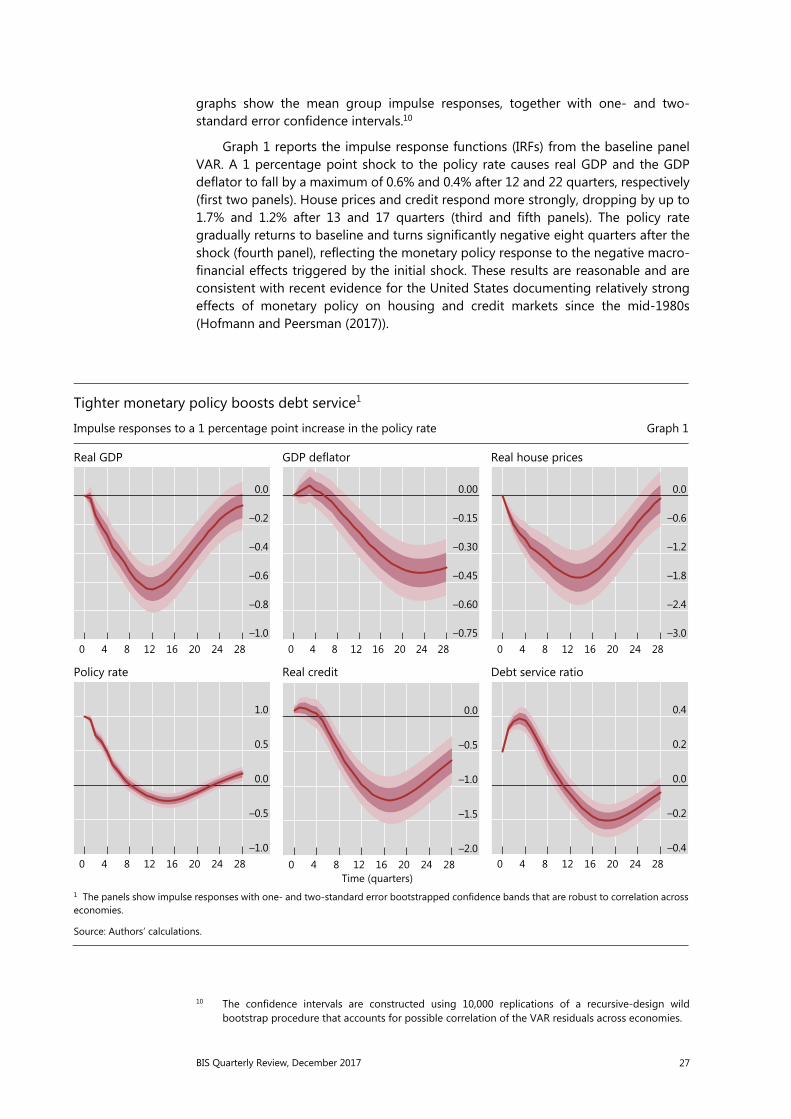
BIS Quarterly Review, December 2017 27
graphs show the mean group impulse responses, together with one- and two-standard error confidence intervals.10
Graph 1 reports the impulse response functions (IRFs) from the baseline panel VAR. A 1 percentage point shock to the policy rate causes real GDP and the GDP deflator to fall by a maximum of 0.6% and 0.4% after 12 and 22 quarters, respectively (first two panels). House prices and credit respond more strongly, dropping by up to 1.7% and 1.2% after 13 and 17 quarters (third and fifth panels). The policy rate gradually returns to baseline and turns significantly negative eight quarters after the shock (fourth panel), reflecting the monetary policy response to the negative macro-financial effects triggered by the initial shock. These results are reasonable and are consistent with recent evidence for the United States documenting relatively strong effects of monetary policy on housing and credit markets since the mid-1980s (Hofmann and Peersman (2017)).
10 The confidence intervals are constructed using 10,000 replications of a recursive-design wild
bootstrap procedure that accounts for possible correlation of the VAR residuals across economies.
Tighter monetary policy boosts debt service1
Impulse responses to a 1 percentage point increase in the policy rate Graph 1
Real GDP GDP deflator Real house prices
Policy rate Real credit Debt service ratio
1 The panels show impulse responses with one- and two-standard error bootstrapped confidence bands that are robust to correlation acrosseconomies.
Source: Authors’ calculations.
0.0
–0.2
–0.4
–0.6
–0.8
–1.02824201612840
0.00
–0.15
–0.30
–0.45
–0.60
–0.752824201612840
0.0
–0.6
–1.2
–1.8
–2.4
–3.02824201612840
1.0
0.5
0.0
–0.5
–1.02824201612840
0.0
–0.5
–1.0
–1.5
–2.02824201612840
Time (quarters)
0.4
0.2
0.0
–0.2
–0.42824201612840

28 BIS Quarterly Review, December 2017
The impact of a monetary policy shock on the DSR is sizeable and significantly positive. A 1 percentage point shock to the policy rate raises the DSR on impact by 0.2 percentage points and by a maximum of 0.4 percentage points after three quarters (Graph 1, sixth panel). Subsequently, the impact starts to decline and becomes significantly negative after about 12 quarters. Qualitatively, the DSR response tracks that of the policy rate, with a lag of about three quarters. Quantitatively, the pass-through of the policy rate shock to the DSR is incomplete, ie the DSR rises at the peak by less than half of the initial shift in the policy rate.
In order to shed more light on how monetary policy affects the DSR, we re-estimate the benchmark model replacing the DSR with its components, namely the effective lending rate on the stock of debt and the debt-to-income ratio. The IRFs of these two variables are shown in Graph 2.
These results suggest that the DSR response is mainly shaped by that of the effective lending rate. In particular, the positive impact of the monetary policy shock on the effective lending rate dominates its negative impact on the debt-to-income ratio in the short term. In the wake of a 1 percentage point tightening shock to the policy rate, the effective lending rate increases by a maximum of 0.4 percentage points after three quarters and then gradually returns to baseline (Graph 2, centre panel), turning moderately negative after about 16 quarters. Thus, the response of the lending rate, like that of the DSR, closely tracks that of the policy rate, with a lag of about three quarters, and the pass-through is incomplete at up to 40% of the initial shift of the policy rate.
Meanwhile, the debt-to-income ratio gradually falls after a tightening, by as much as 1.3 percentage points after 18 quarters (Graph 2, right-hand panel). To some extent, the decline counteracts the impact of the increase in the lending rate on the DSR. The medium-term decline in the debt-to-income ratio ultimately translates into a decline in the DSR beyond the three-year horizon.
Monetary policy affects DSRs primarily through lending rates1
Impulse responses to a 1 percentage point increase in the policy rate Graph 2
Debt service ratio Effective lending rate Debt-to-income ratio
1 The panels show impulse responses with one- and two-standard error bootstrapped confidence bands that are robust to correlation acrosseconomies.
Source: Authors’ calculations.
0.4
0.2
0.0
–0.2
–0.42824201612840
0.4
0.2
0.0
–0.2
–0.42824201612840
Time (quarters)
0.0
–0.5
–1.0
–1.5
–2.02824201612840

BIS Quarterly Review, December 2017 29
The role of debt
The results of the previous section are based on combined data for 18 economies. They reveal that a higher monetary policy rate tends to increase the DSR over a horizon of two years, because of its impact on the lending rate. Similar results hold at the individual economy level (Appendix Graph A1). However, the size of this effect differs across economies. Similarly, while tighter monetary policy almost always slows real GDP growth, this effect is stronger for some economies than for others (Appendix Graph A2).
One potential reason for these differences is the cross-country variation in private non-financial sector indebtedness.11 By construction, the magnitude of the impact of a change in policy rates on the DSR should, for a given pass-through to lending rates, depend on the (initial) debt-to-income ratio. In other words, when the private sector is more leveraged, a given change in the lending rate should have a larger effect on the DSR. If there is a debt service channel of monetary transmission, this could also strengthen the consequent effects on the macroeconomy.
To analyse this hypothesis in more detail, we divide our sample into two groups of nine economies, according to their average private non-financial sector debt-to-GDP ratios over the sample period.12 We then estimate panel VARs for the high- and low-debt groups and compare the IRFs. 13 Graph 3 shows the IRFs of the two groups, while Appendix Graph A3 shows the estimated differences between these IRFs.
The data confirm our intuition. The peak impact on the DSR is around 0.2 percentage points higher for the high-debt economies, and the difference is statistically significant (Graph 3 and Appendix Graph A3, sixth panel). By contrast, the impact on the effective lending rate and the debt-to-income ratio is quite similar across both groups. The difference between the impulse responses of the DSR components is statistically also not significant (Appendix Graph A3). This implies that the stronger response of the DSR to monetary policy in the high-debt economies is driven by the higher initial debt level, rather than by the changes in the DSR components following the monetary policy shock.
11 Another possible reason is the flexibility of the effective lending rate, determined by the maturity
structure of debt contracts (short- vs long-term) and the adjustability of lending rates (fixed vs variable). We do not assess the relevance of this potential factor here because the information on lending rate flexibility is rather sketchy. For instance, information on the adjustability of lending rates is generally available only for the household sector and for specific points in time (Borio (1995), CGFS (2006)). BIS (1995) finds that the distinction between fixed and flexible lending rates was important in explaining cross-country differences in monetary transmission. More recently, Calza et al (2013) report VAR-based evidence suggesting that monetary transmission to house prices, consumption and residential investment is stronger in economies with predominantly variable rate – as opposed to fixed rate – mortgage contracts.
12 Debt-to-GDP is preferred to debt-to-income of the private non-financial sector because it also accounts for the share of the private sector in total GDP. The group of high-debt economies comprises Canada, Denmark, Hong Kong SAR, Japan, the Netherlands, Norway, Sweden, Switzerland and the United States; the low-debt economies are Australia, Belgium, Finland, France, Germany, Italy, South Africa, Spain and the United Kingdom.
13 The confidence intervals are constructed as before (see footnote 10). The joint estimation of the VARs allows us to construct confidence intervals for the differences between the high-debt and low-debt economies’ IRFs.

30 BIS Quarterly Review, December 2017
We also observe much stronger effects on economic activity and the price level in economies where private non-financial sector debt levels are higher. The peak responses of both real GDP and the GDP deflator are more than 0.4 percentage points
Monetary transmission is stronger in economies where debt is high1
Impulse responses to a 1 percentage point increase in the policy rate Graph 3
Real GDP GDP deflator Real house prices
Policy rate Real credit Debt service ratio
Effective lending rate Debt-to-income ratio
1 The panels show impulse responses with one-standard error bootstrapped confidence bands that are robust to correlation acrosseconomies.
Source: Authors’ calculations.
0.0
–0.3
–0.6
–0.9
–1.22824201612840
0.0
–0.2
–0.4
–0.6
–0.82824201612840
0
–1
–2
–3
–42824201612840
1.0
0.5
0.0
–0.5
–1.02824201612840
0.0
–0.5
–1.0
–1.5
–2.02824201612840
0.4
0.2
0.0
–0.2
–0.42824201612840
0.4
0.2
0.0
–0.22824201612840
0
–1
–2
–32824201612840
Time (quarters)
Point estimate 16th–84th percentile
High-debt countries:
Low-debt countries:

BIS Quarterly Review, December 2017 31
larger in high-debt economies. The estimated differences are economically meaningful, ie the effects on real GDP are roughly double, and statistically highly significant (Graph 3 and Appendix Graph A3, first two panels). The impacts on house prices and credit are also significantly larger. In the high-debt economies, the drop in house prices is 1.3 percentage points larger than in the low-debt group, while that of credit is 0.6 percentage points larger (Graph 3 and Appendix Graph A3, third and fifth panels).14
Graph 4 confirms that monetary policy has a stronger impact in economies where private debt is high. This graph compares the maximum impact of tighter policy on real GDP in the individual economies (on the vertical axis) with their average private non-financial sector debt-to-GDP levels during the sample period (on the horizontal axis). The correlation is negative and significant: GDP decreases more after a contractionary monetary policy shock in economies with high debt.
A possible explanation for the stronger effects of monetary policy when debt is high is the larger change in the DSR following a monetary policy shock. Specifically, a larger shift in the DSR implies a larger shift in the disposable income (that is, the income that remains after servicing debt) of debtors, who typically have a higher marginal propensity to consume than savers. Put differently, there might be a debt service channel of monetary transmission at play that enhances the effectiveness of monetary policy in countries with higher debt levels.
The analysis comes with caveats. The correlations between the strength of monetary transmission and the level of debt-to-GDP are obviously based on relatively few observations (economies). Moreover, these correlations do not control for the role of other factors that may be relevant for monetary transmission, such as differences in financial structure or the degree of economic and financial openness. That said, it is a first cross-country analysis of the role of debt in monetary transmission that could be developed further in future research.
14 These results also hold when we exclude individual countries from the analysis, and when we change
the groupings, eg comparing the six highest and six lowest debt-to-GDP economies.
Higher debt coincides with a larger impact of monetary policy on GDP1 Graph 4
1 Maximum impulse responses of real GDP, in per cent, to a 1 percentage point increase in the policy rate for 18 economies. The regression equation shows standard errors in parentheses. 2 Total private non-financial debt-to-GDP ratio on the horizontal axis.
Source: Authors’ calculations.
–0.5
–1.0
–1.5
–2.0
–2.520017515012510075
Max
imum
impa
ct o
n re
al G
DP
Debt-to-GDP (%)2
y = 0.0186 – 0.0062x (0.3763) (0.0032)where R2= 0.166

32 BIS Quarterly Review, December 2017
Conclusions
Our results confirm that a potentially important, and underappreciated, channel through which monetary policy may affect the economy is its impact on private sector debt service ratios, as previously suggested by Juselius et al (2017). A change in the monetary policy stance, measured here as a monetary policy shock identified in a standard vector autoregression, triggers a significant and persistent change in the DSR in the same direction. A monetary tightening increases the DSR; an easing lowers it. This effect is the result of the positive impact of monetary policy on effective lending rates, which dominates a negative effect on debt-to-income ratios.
We also find that the effects of monetary policy on DSRs, as well as on economic activity, the price level, credit and housing markets, are significantly larger in countries with high private non-financial sector debt. The level of debt and the corresponding response of the DSR might therefore be important for the transmission of monetary policy. Potentially fruitful areas for future research include the precise nature of these effects as well as how they differ across countries, states of the economy, or tightening and easing episodes.
These findings suggest that the extraordinary monetary accommodation engineered by leading central banks in the wake of the Great Financial Crisis may have alleviated debt service burdens in highly indebted countries. This might have played an important role in dampening the after-effects of the crisis and in supporting the recovery. At the same time, our results also suggest that persistent high debt levels may represent a complicating factor in the ongoing or prospective normalisation of monetary policy in many economies. We find that economies with high debt are more interest rate-sensitive, so that a policy tightening could have stronger adverse macroeconomic effects than otherwise. Some observers argue that this could induce central banks to pursue the normalisation in a more cautious way, which could in turn raise the risk of a “debt trap” (eg Borio and Disyatat (2014) and Juselius et al (2017)): high debt makes it harder to raise rates, but keeping rates low induces further debt accumulation. A deeper analysis of these normative considerations is, however, beyond the scope of this special feature and is left for future research.
BIS Quarterly Review, December 2017 33
References
Albuquerque, B (2017): “One size fits all? Monetary policy and asymmetric household debt cycles in US states”, Ghent University Working Papers, no 2017/937, May.
Alpanda, S and S Zubairy (2017): “Household debt overhang and transmission of monetary policy”, Texas A&M University, mimeo.
Auclert, A (2017): “Monetary policy and the redistribution channel”, NBER Working Papers, no 23451.
Bank for International Settlements (1995): “Financial structure and the monetary policy transmission mechanism”, BIS Papers, no 0, March.
Bauer, G and E Granziera (2017): “Monetary policy, private debt and financial stability risks”, International Journal of Central Banking, vol 13, pp 337–73.
Borio, C (1995): “The structure of credit to the non-government sector and the transmission mechanism of monetary policy: a cross-country comparison”, BIS Working Papers, no 24, April.
Borio, C and P Disyatat (2014): “Low interest rates and secular stagnation: is debt a missing link?”, VOX, June.
Calza, A, T Monacelli and L Stracca (2013): “Housing finance and monetary policy”, Journal of the European Economic Association, vol 11, pp 101–22.
Christiano, L, M Eichenbaum and C Evans (1996): “The effects of monetary policy shocks: evidence from the flow of funds”, The Review of Economics and Statistics, vol 78, no 1, pp 16–34.
——— (1999): “Monetary policy shocks: what have we learned and to what end?”, in J Taylor and M Woodford (eds), Handbook of Macroeconomics, vol (1)A, Amsterdam: Elsevier Science, pp 65–148.
Cloyne, J, C Ferreira and P Surico (2016): “Monetary policy when households have debt: new evidence on the transmission mechanism”, Bank of England, Working Papers, no 589, April.
Committee on the Global Financial System (2006): “Housing finance in the global financial market”, CGFS Papers, no 26, January.
Di Maggio, M, A Kermani, B Keys, T Piskorski, R Ramcharan, A Seru and V Yao (2017): ”Interest rate pass-through: mortgage rates, household consumption, and voluntary deleveraging”, American Economic Review, vol 107, no 11, pp 3550–88.
Di Maggio, M, A Kermani and R Ramcharan (2015): “Monetary policy pass-through: household consumption and voluntary deleveraging”, Society for Economic Dynamics 2015 Meeting Papers, no 256.
Drehmann, M, A Illes, M Juselius and M Santos (2015): “How much income is used for debt payments? A new database for debt service ratios”, BIS Quarterly Review, September 2015, Box 2, p 98.
Drehmann, M and M Juselius (2012): “Do debt service costs affect macroeconomic and financial stability?”, BIS Quarterly Review, September, pp 21–35.
——— (2014): "Evaluating early warning indicators of banking crises: satisfying policy requirements", International Journal of Forecasting, vol 30, no 3, pp 759–80 (also published as BIS Working Paper no 421).

34 BIS Quarterly Review, December 2017
Drehmann, M, M Juselius and A Korinek (2017): “Accounting for debt service: the painful legacy of credit booms”, BIS Working Papers, no 645, June.
Eggertsson, G and P Krugman (2012): “Debt, deleveraging, and the liquidity trap: a Fisher-Minsky-Koo approach”, Quarterly Journal of Economics, vol 127, no 3, pp 1469–1513.
Hofmann, B and G Peersman (2017): “Monetary policy transmission and trade-offs in the United States: old and new”, BIS Working Papers, no 649, July.
Jordà, Ò, M Schularick and A Taylor (2013): “When credit bites back”, Journal of Money, Credit and Banking, vol 45, issue s2, pp 3–28.
Juselius, M, C Borio, P Disyatat and M Drehmann (2017): “Monetary policy, the financial cycle, and ultra-low interest rates”, International Journal of Central Banking, vol 13, no 3, pp 55–90.
Juselius, M and M Drehmann (2015): “Leverage dynamics and the real burden of debt”, BIS Working Papers, no 501, May.
Kaplan, G and G Violante (2014): “A model of the consumption response to fiscal stimulus payments”, Econometrica, vol 82, no 4, pp 1199–1239.
Koo, R (2009): The holy grail of macroeconomics – lessons from Japan’s Great Recession, John Wiley & Sons.
La Cava, G, H Hughson and G Kaplan (2016): “The household cash flow channel of monetary policy”, Reserve Bank of Australia, Research Discussion Papers, no 2016–12, December.
Lombardi, M, M Mohanty and I Shim (2017): “The real effects of household debt in the short and long run”, BIS Working Papers, no 607, January.
Mian, A and A Sufi (2014): House of debt: how they (and you) caused the Great Recession, and how we can prevent it from happening again, University of Chicago Press.
Mian, A, A Sufi and E Verner (2017): “Household debt and business cycles worldwide”, Quarterly Journal of Economics, forthcoming.
Sims, C (1992): “Interpreting the macroeconomic time series facts: the effects of monetary policy”, European Economic Review, vol 36, no 5, pp 975–1000.
Sims, C, J Stock and M Watson (1990): “Inference in linear time series models with some unit roots”, Econometrica, vol 58, no 1, pp 113–44.
Tobin, J (1982): Asset accumulation and economic activity: reflections on contemporary macroeconomic theory, University of Chicago Press.

BIS Quarterly Review, December 2017 35
Monetary policy impact on debt service ratios in individual economies1
Impulse responses to a 1 percentage point increase in the policy rate Graph A1
Australia Belgium Canada Switzerland
Germany Denmark Spain Finland
France United Kingdom Hong Kong SAR Italy
Japan Netherlands Norway Sweden
United States South Africa
1 The panels show impulse responses with one- and two-standard error bootstrapped confidence bands.
Source: Authors’ calculations.
0.50
0.25
0.00
–0.25
–0.50
–0.752820124
0.30
0.15
0.00
–0.15
–0.30
–0.452820124
0.4
0.2
0.0
–0.2
–0.4
–0.62820124
0.4
0.2
0.0
–0.2
–0.4
–0.62820124
0.6
0.3
0.0
–0.3
–0.62820124
0.8
0.4
0.0
–0.4
–0.82820124
0.8
0.4
0.0
–0.4
–0.82820124
0.4
0.2
0.0
–0.2
–0.42820124
0.2
0.1
0.0
–0.1
–0.2
–0.32820124
0.50
0.25
0.00
–0.25
–0.50
–0.752820124
0.8
0.4
0.0
–0.4
–0.8
–1.22820124
0.4
0.2
0.0
–0.2
–0.4
–0.62820124
0.5
0.0
–0.5
–1.0
–1.5
–2.02820124
1.0
0.5
0.0
–0.5
–1.0
–1.52820124
1.5
1.0
0.5
0.0
–0.5
–1.02820124
0.8
0.4
0.0
–0.4
–0.8
–1.22820124
0.5
0.0
–0.5
–1.0
–1.52820124
Time
0.4
0.2
0.0
–0.2
–0.42820124
(quarters)
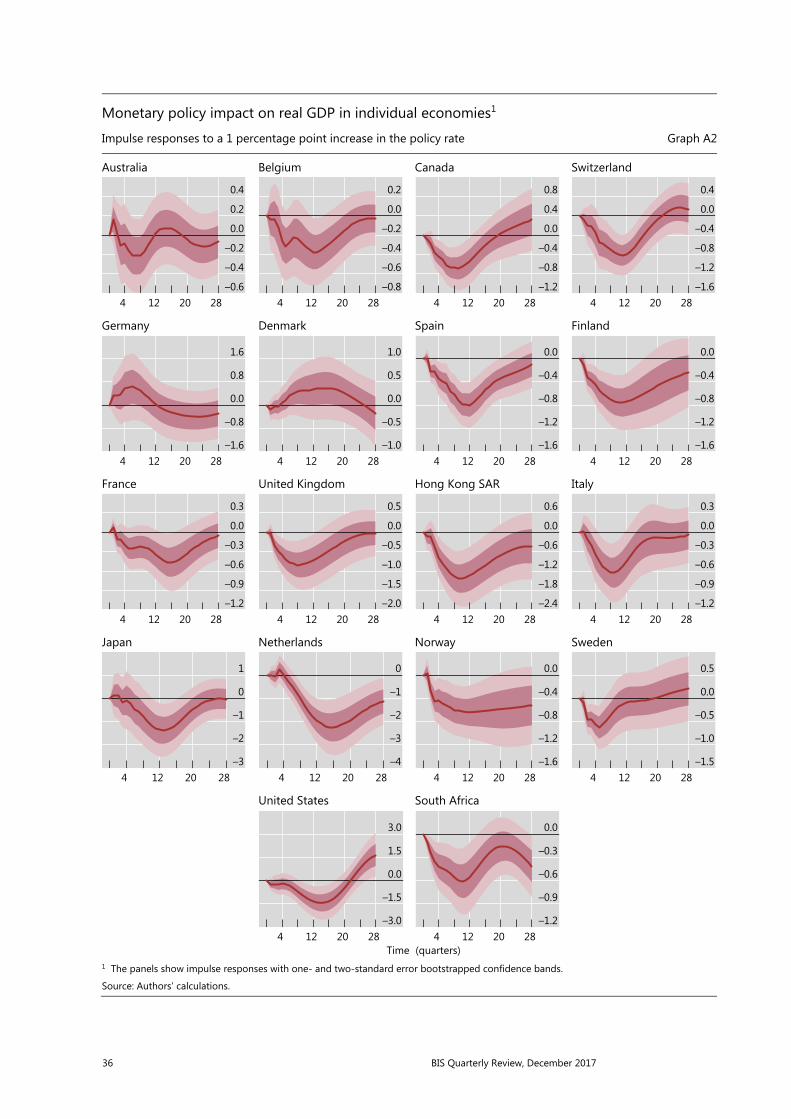
36 BIS Quarterly Review, December 2017
Monetary policy impact on real GDP in individual economies1
Impulse responses to a 1 percentage point increase in the policy rate Graph A2
Australia Belgium Canada Switzerland
Germany Denmark Spain Finland
France United Kingdom Hong Kong SAR Italy
Japan Netherlands Norway Sweden
United States South Africa
1 The panels show impulse responses with one- and two-standard error bootstrapped confidence bands.
Source: Authors’ calculations.
0.4
0.2
0.0
–0.2
–0.4
–0.62820124
0.2
0.0
–0.2
–0.4
–0.6
–0.82820124
0.8
0.4
0.0
–0.4
–0.8
–1.22820124
0.4
0.0
–0.4
–0.8
–1.2
–1.62820124
1.6
0.8
0.0
–0.8
–1.62820124
1.0
0.5
0.0
–0.5
–1.02820124
0.0
–0.4
–0.8
–1.2
–1.62820124
0.0
–0.4
–0.8
–1.2
–1.62820124
0.3
0.0
–0.3
–0.6
–0.9
–1.22820124
0.5
0.0
–0.5
–1.0
–1.5
–2.02820124
0.6
0.0
–0.6
–1.2
–1.8
–2.42820124
0.3
0.0
–0.3
–0.6
–0.9
–1.22820124
1
0
–1
–2
–32820124
0
–1
–2
–3
–42820124
0.0
–0.4
–0.8
–1.2
–1.62820124
0.5
0.0
–0.5
–1.0
–1.52820124
3.0
1.5
0.0
–1.5
–3.02820124
Time
0.0
–0.3
–0.6
–0.9
–1.22820124
(quarters)

BIS Quarterly Review, December 2017 37
Differences in monetary transmission between high- and low-debt economies1
Differences in impulse responses to a 1 percentage point increase in the policy rate Graph A3
Real GDP GDP deflator Real house prices
Policy rate Real credit Debt service ratio
Effective lending rate Debt-to-income ratio
1 The panels show differences between the impulse responses of high- and low-debt economies with one- and two-standard error bootstrapped confidence bands that are robust to correlation across countries.
Source: Authors’ calculations.
0.25
0.00
–0.25
–0.50
–0.75
–1.002824201612840
0.2
0.0
–0.2
–0.4
–0.6
–0.82824201612840
1.8
0.9
0.0
–0.9
–1.8
–2.72824201612840
0.2
0.1
0.0
–0.1
–0.2
–0.32824201612840
0.4
0.0
–0.4
–0.8
–1.2
–1.62824201612840
0.4
0.2
0.0
–0.2
–0.4
–0.62824201612840
0.2
0.1
0.0
–0.1
–0.2
–0.32824201612840
0.5
0.0
–0.5
–1.0
–1.5
–2.02824201612840
Time (quarters)


BIS Quarterly Review, December 2017 39
Household debt: recent developments and challenges1
The responsiveness of aggregate expenditure to shocks depends on the level and interest rate sensitivity (duration) of household debt, as well as on the liquidity of the assets it finances. Household-level spending adjustments are more likely to be amplified if debt is concentrated among households with limited access to credit or with less scope for self-insurance. The way in which household indebtedness affects the sensitivity of aggregate expenditure matters for both macroeconomic and financial stability. Financial institutions can suffer balance sheet distress from both direct and indirect exposure to the household sector. From a macroeconomic stability viewpoint, monetary transmission is the key issue. In a high-debt economy, interest rate hikes could be more contractionary than cuts are expansionary. These considerations point to a complementarity between current macroprudential and future monetary policy.
JEL classification: E21, E24, E52, E58, D15, G01.
Ten years after breakdowns in housing finance markets plunged the financial system into crisis, household debt levels are again rising, with debt-to-GDP ratios reaching historical highs in several countries (Graph 1). Central banks are increasingly concerned that this may pose a threat to macroeconomic and financial stability (eg Reserve Bank of Australia (2017), Bank of Canada (2017), Bank of England (2017)).
After discussing key developments in household debt since the Great Financial Crisis (GFC), this special feature seeks to highlight some of the mechanisms through which household debt may threaten both macroeconomic and financial stability.
Debt lets households smooth shocks and invest in high-return assets such as housing or education, raising average consumption over their lifetimes. However, high household debt can make the economy more vulnerable to disruptions, potentially harming growth. As aggregate consumption and output shrink, the
1 This special feature draws on material prepared for the Committee on the Global Financial System.
Bernadette Donovan (Reserve Bank of Australia), Alexander Ueberfeldt (Bank of Canada), Peter van Santen (Sveriges Riksbank), Gavin Wallis (Bank of England) and Seung Sik Byun (Bank of Korea) provided a wealth of useful material about their respective jurisdictions, as well as insightful comments on earlier drafts. Special thanks to Marco Lombardi for sharing code. Thanks also to Claudio Borio, Stijn Claessens, Benjamin Cohen, Dietrich Domanski, Mathias Drehmann, Gianni Lombardo, Hyun Song Shin, Kostas Tsatsaronis and Grant Turner for comments and helpful discussions. Anamaria Illes provided outstanding research assistance. Any errors and omissions are solely the author’s responsibility. The views expressed here are those of the author and do not necessarily reflect those of the BIS.
Anna Zabai

40 BIS Quarterly Review, December 2017
likelihood of systemic banking distress could increase, since banks hold both direct and indirect credit risk exposures to the household sector.
This special feature starts by discussing recent developments in household debt, focusing on trends, levels, and composition but also considering buffers and debt burdens. The following two sections discuss the implications for macroeconomic and financial stability, as sketched out above. They also provide evidence that high household debt can indeed slow economic growth in the medium term, possibly increasing the likelihood of systemic distress. A concluding section highlights some of the issues relevant for monetary and macroprudential policies.
How has household debt developed since the GFC?
Countries can be broadly classified into four groups, based on the level and trend of household debt as a ratio to GDP (debt ratio). An especially significant group comprises those countries with debt ratios that are both high (eg over 60% of GDP on average since the GFC) and trending higher (Graph 1, first panel).2 Among these, the debt ratio now exceeds 120% in both Australia and Switzerland. Countries in the second group also have high household debt relative to GDP, but the debt ratio trend seems to have either levelled off or declined in recent years (Graph 1, second panel).
2 Studies of financial development have found the existence of a tipping point in financial deepening.
When aggregate credit exceeds a certain threshold (between 80 and 100% of GDP), the relationship between credit and long-term GDP growth turns from positive to negative (eg Cecchetti and Kharroubi (2012), Arcand et al (2015)). A recent analysis (IMF (2017)) suggests that a tipping point may exist also in the relationship between household credit and long-term GDP growth. The exercise finds that the maximum positive impact is when household debt is between 36 and 70% of GDP. The threshold chosen for the grouping of countries in this special feature – 60% of GDP – is roughly in the middle of this interval.
Household debt since the Great Financial Crisis
As a percentage of GDP Graph 1
High and rising High and flat/falling Low and rising Low and flat/falling
Source: BIS.
120
100
80
60
40
20
01715131109
AustraliaCanadaSwitzerland
SwedenKoreaNorway
120
100
80
60
40
20
01715131109
SpainUnited KingdomUnited StatesNetherlands
120
100
80
60
40
20
01715131109
BelgiumBrazilFrance
ChinaSingapore
120
100
80
60
40
20
01715131109
Euro areaGermanyItaly
JapanIndiaMexico

BIS Quarterly Review, December 2017 41
The two right-hand panels in Graph 1 relate to countries with average household debt ratios below 60% in the period since 2007. Among these, the third panel shows countries where debt ratios have been trending up during the past 10 years, while the fourth displays some where debt has fallen.
The composition of household debt is heavily skewed towards housing-related debt (Table 1, columns 1 and 2). Mortgages make up the lion’s share of debt (between 62 and 97% in the group of countries considered here), a share that has remained broadly stable since the GFC. Households may take out mortgages to buy not only a primary residence but also properties that are rented out.3
In order to assess the implications of elevated household debt levels, it is crucial to have a sense of whether households can bear the resulting debt burdens without resorting to large adjustments in consumption should circumstances worsen.
To that end, it is important to establish whether households have been accumulating buffers that can help smooth unexpected adverse changes. The left-hand panel of Graph 2 reports household “leverage”, defined here as the ratio of household debt to financial assets. Leverage is flat for countries in the first and third groups from Graph 1, suggesting that households in countries with rising debt have also seen the value and amount of their assets rise. Households in the second group, where debt is high but falling, seem to have made the most significant progress in repairing balance sheets, with leverage dropping more than 10 percentage points in the 10 years since the GFC.
3 This investment option is particularly popular in Korea, where almost 80% of rented property is
owned by households. In Australia, the share of lending to investors has been rising in recent years.
Household debt buffers and burdens Graph 2
Household leverage1 Household debt service ratio2 Per cent Percentage points
High and rising = Australia, Canada, Korea, Norway, Sweden and Switzerland; high and flat/falling = the Netherlands, Spain, the United Kingdom and the United States; low and rising = Belgium, Brazil, China, France and Singapore; low and flat/falling = the euro area, Germany,India, Italy, Japan and Mexico.
1 Household sector financial assets as a share of household debt. Simple average across groups. Data for Korea start Q1 2008 and end Q4 2016, data for Switzerland end Q4 2015; no data available for BR, CN, IN, MX and SG. 2 Difference of DSRs for the household sector from country-specific long-run averages since 1999. No data available for BR, CH, CN, EA, IN, MX and SG.
Sources: Datastream; national data; BIS; BIS calculations.
40
30
20
10
017161514131211100908
High and risingHigh and flat/falling
2
1
0
–1
–217161514131211100908
Low and risingLow and flat/falling

42 BIS Quarterly Review, December 2017
The size of household debt burdens matters too. This is best measured by the ratio of interest payments and amortisation to income – the debt service ratio (DSR; Drehmann et al (2015)). In countries where household debt has been on the rise (groups 1 and 3), DSRs have consistently exceeded their long-term averages in the 10 years since the GFC (Graph 2, right-hand panel). The DSR dynamics, however, differ across the two groups. While the DSR has been on an upward trend in group 3, its level has been more volatile in group 1. As shown in Table 1, countries in group 1 are mostly “adjustable rate” countries, while countries in group 3 are mostly “fixed rate” (column 3). This observation suggests that, while DSRs in the latter group have been pushed up by credit growth, falling interest rates have played a bigger role in the
Household mortgage debt: key features Table 1
Country Mortgage share (in per cent)
Main interest rate type
Equity release products
Full recourse Max LTV1 Retail funding2
2007 2017
Group 1: High and rising
Australia 86 92 Variable Used Yes 100 Other
Canada 76 75 Mixed Used Yes 95 Retail deposit
Korea … 76 Variable … No 70 Retail deposit
Norway 97 97 Variable Used Yes 85 Retail deposit
Sweden 83 87 Variable Used Yes 95 Other
Switzerland ... ... Fixed Not used Yes 80 Other
Group 2: High and flat/falling
Netherlands 94 97 Fixed Used Yes 125 Retail deposit
Spain 95 96 Variable Limited use Yes 100 Retail deposit
United Kingdom
80 78 Variable Used Yes 110 Retail deposit
United States 80 72 Mixed Used Varies by state3 100 Other
Group 3: Low and rising
Belgium 78 83 Fixed Not used Yes 100 Retail deposit
Brazil … … Fixed … No 90 Retail deposit
China … … Variable … No 80 Retail deposit
France 82 86 Fixed Not used Yes 100 Retail deposit
Singapore … … Variable … Yes 80 Other
Group 4: Low and flat/falling
Germany 95 97 Fixed Not used Yes 80 Retail deposit
India … … Mixed … No 110 Retail deposit
Italy 91 92 Variable Not used Yes 80 Retail deposit
Japan 62 67 Mixed Not used Yes 80 Retail deposit
Mexico … … Variable … No 100 Other 1 Maximum observed LTV, often coincident with legal limit. 2 Main funding model (ie retail deposit, securitisation, covered bonds, wholesalemarkets). 3 See Ghent and Kudlyak (2011).
Sources: Calza et al (2013); Cerutti et al (2015); Ghent and Kudlyak (2011); national data.
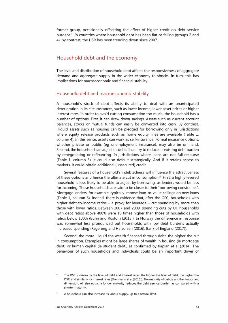
BIS Quarterly Review, December 2017 43
former group, occasionally offsetting the effect of higher credit on debt service burdens.4 In countries where household debt has been flat or falling (groups 2 and 4), by contrast, the DSR has been trending down since 2007.
Household debt and the economy
The level and distribution of household debt affects the responsiveness of aggregate demand and aggregate supply in the wider economy to shocks. In turn, this has implications for macroeconomic and financial stability.
Household debt and macroeconomic stability
A household’s stock of debt affects its ability to deal with an unanticipated deterioration in its circumstances, such as lower income, lower asset prices or higher interest rates. In order to avoid cutting consumption too much, the household has a number of options. First, it can draw down savings. Assets such as current account balances, stocks or mutual funds can easily be converted into cash. By contrast, illiquid assets such as housing can be pledged for borrowing only in jurisdictions where equity release products such as home equity lines are available (Table 1, column 4). In this sense, assets can work as self-insurance. Formal insurance options, whether private or public (eg unemployment insurance), may also be on hand. Second, the household can adjust its debt. It can try to reduce its existing debt burden by renegotiating or refinancing. In jurisdictions where loans are not full-recourse (Table 1, column 5), it could also default strategically. And if it retains access to markets, it could obtain additional (unsecured) credit.
Several features of a household’s indebtedness will influence the attractiveness of these options and hence the ultimate cut in consumption.5 First, a highly levered household is less likely to be able to adjust by borrowing, as lenders would be less forthcoming. These households are said to be closer to their “borrowing constraints”. Mortgage lenders, for example, typically impose loan-to-value ceilings on new loans (Table 1, column 6). Indeed, there is evidence that, after the GFC, households with higher debt-to-income ratios – a proxy for leverage – cut spending by more than those with lower ratios. Between 2007 and 2009, spending cuts by UK households with debt ratios above 400% were 10 times higher than those of households with ratios below 100% (Bunn and Rostom (2015)). In Norway the difference in response was somewhat less pronounced but households with low debt burdens actually increased spending (Fagereng and Halvorsen (2016), Bank of England (2017)).
Second, the more illiquid the wealth financed through debt, the higher the cut in consumption. Examples might be large shares of wealth in housing (ie mortgage debt) or human capital (ie student debt), as confirmed by Kaplan et al (2014). The behaviour of such households and individuals could be an important driver of
4 The DSR is driven by the level of debt and interest rates: the higher the level of debt, the higher the
DSR, and similarly for interest rates (Drehmann et al (2015)). The maturity of debt is another important dimension. All else equal, a longer maturity reduces the debt service burden as compared with a shorter maturity.
5 A household can also increase its labour supply, up to a natural limit.

44 BIS Quarterly Review, December 2017
aggregate expenditure where high debt levels coincide with a large share of wealth locked up in residential property, as in Sweden. Similarly, in Australia, the liquid pre-payment buffers on mortgage-offset accounts are heavily concentrated on older
Accounting for the increase in the stock of debt: credit demand vs credit supply
Rising household debt can reflect either stronger credit demand or an increased supply of credit from lenders, or some combination of the two.
Unconstrained households can borrow in order to smooth consumption before an anticipated increase in income or after an unexpected temporary drop in income (eg illness, accidents, short-term unemployment). In addition, households borrow to finance investment in illiquid assets with high long-term returns such as housing (Kaplan et al (2014)). Credit demand might rise because households are optimistic about income prospects, or because costs (interest rates) are low. The post-Great Financial Crisis period has seen extraordinary monetary accommodation, very low borrowing rates and low returns on safe assets. This combination has lifted debt-financed demand for housing, either for own use or as an investment (eg in Germany, property has recently been referred to as “concrete gold”).
Structural factors such as demographic shifts could also be playing a supporting role. Population growth could have contributed to the rise in credit in Australia and Canada. Structural factors combine with demand factors in Korea: returns on real estate investments have been especially high, encouraging households close to retirement to borrow to invest in buy-to-let properties with the aim of generating income for old age.
Favourable supply conditions can also boost credit to households. In Australia, for instance, heightened competition among lenders seems to have resulted in a relaxation of lending standards. There is some evidence that this may also matter for UK consumer credit (Bank of England (2017)). In Korea, solvency (loan-to-value ratios) and affordability (debt-to-income ratios) requirements on new loans have been relaxed as part of a broader easing of real estate regulation. In the United States, the government has supported the secondary mortgage market through its long-standing implicit guarantee of debt issued by government-sponsored enterprises. In addition, the post-crisis world has been marked by greater emphasis on a more traditional, retail-oriented approach to banking.
Table A presents evidence that supply factors may have been more important than demand in driving household credit in some jurisdictions. The coefficients are computed following Mian et al (2017), who estimate a proxy vector autoregression (VAR) in two steps. A negative (positive) coefficient implies that increases in credit to households that are not explained by the dynamics of GDP growth, credit to households itself and credit to non-financial firms are associated with narrow (wide) mortgage spreads, which are in turn more likely to be correlated with outward shifts in credit supply than in credit demand. The results shown in column 1 use the sample of countries listed in Table 1. These results are qualitatively consistent with the findings of Mian et al (2017), who consider a broader range of countries (column 2), although the estimates are not as precise because of the smaller sample size.
Supply vs demand factors in driving credit Table A
Dependent variable: Household debt
(1) (2)
Mortgage-sovereign spread –0.217 –0.341** (0.153) (0.101)
Observations 358 580
Notes: this table presents results from the second step of the following procedure. First, OLS is used to estimate the reduced-form VAR residuals of a three-equation VAR in GDP, credit to households and credit to non-financial firms. Then the residuals of the household debt equation are regressed on the mortgage/sovereign spread (treated as instrument). See Mian et al (2017), Table VI. The sample in column (1) is an (unbalanced) panel of the following countries: Australia, Belgium, Brazil, Canada, Germany, France, Hong Kong SAR, Italy, Japan, Korea, Mexico, the Netherlands, Singapore, Spain, Sweden, Switzerland, the United Kingdom, the United States and the euro area. The VAR is estimated on the full sample (annual data ranging from 1966 to 2012), but the credit supply shock is identified on the subsample where the instrument (the mortgage spread) is not missing. Column (2) is repeated from Mian et al (2017).
Between 2012 and 2016, the number of households in the 60+ age group owning buy-to-let properties has grown by about 50%, and accounts for most of the growth in such investments. The investments are largely debt-financed.

BIS Quarterly Review, December 2017 45
mortgages with less time to maturity.6 For one third of mortgages, available repayment buffers cover no more than one month’s worth of loan payments (Reserve Bank of Australia (2017)).7
Third, the interest rate sensitivity of a household’s debt service burden is likely to matter. The greater the interest rate sensitivity – or duration – of a household’s liabilities relative to that of its assets, and the shorter the maturity of these liabilities, the larger the impact on consumption (Auclert (2017)). This effect would be bigger in countries with more debt at variable rates.
Finally, high debt (relative to assets) can make a household less mobile, and hence less able to adjust by finding a new or better job in another town or region. Homeowners may be tied down by mortgages on properties that have depreciated in value, especially those that are underwater (ie worth less than the loan balance). The trend of homeownership tenure in the United States is consistent with this possibility. The median homeownership tenure there was about four years over the period 2000–07, but it has been rising steadily since and has now approximately doubled.8
These household-level observations have implications for aggregate demand and aggregate supply. From an aggregate demand perspective, the distribution of debt across households can amplify any drop in consumption. Notable examples include high debt concentration among households with limited access to credit (ie close to borrowing constraints) or less scope for self-insurance (ie low liquid balances).
Since poorer households are more likely to face these credit and liquidity constraints, an economy’s vulnerability to amplification can be assessed by looking at the distribution of debt by income and wealth. In many countries, most debt is held by households in the top quintiles of the income and wealth distribution. In Canada, for example, the two top quintiles hold approximately 50% of total and mortgage debt (Graph 3, left-hand panel). In Australia, households in the top income brackets tend to have substantially higher debt ratios than those at the bottom of the distribution (eg in 2014, the top two quintiles had debt ratios of about 200%, while the bottom two had ratios of about 50%, centre panel). This is not necessarily the case everywhere, however. In Sweden, the debt ratio is more equally distributed across the income distribution (right-hand panel).
Moreover, all else equal, one would expect the impact of indebtedness on monetary transmission to be larger in economies where household debt is high and adjustable-rate debt is more prevalent (see also Hofmann and Peersman (2017, this issue) and BIS (1995)). Monetary policy is likely to have asymmetrical effects in a high-debt economy, meaning that interest rate hikes cause aggregate expenditure to contract more than cuts would cause it to expand (Sufi (2015)). This is because credit-constrained borrowers cut consumption a lot in response to interest rate hikes, as their debt service burdens increase. However, they do not expand it as much in
6 Funds deposited on an offset account are netted against the borrower’s outstanding mortgage
balance for the purposes of calculating interest on the loan. A mortgage offset account works like a demand deposit account, so that accumulated funds are available for withdrawal or for purchasing goods and services.
7 See Chapter 2, Graph 2.8.
8 See www.attomdata.com/news/heat-maps/q2-2017-home-sales-report/.

46 BIS Quarterly Review, December 2017
response to cuts of equal magnitude. They prefer to save an important fraction of their gains so as to avoid being credit-constrained again in the future (Di Maggio et al (2017)). The asymmetry is likely to increase as the duration of household liabilities shortens, as this boosts the impact of interest rate hikes on their debt service burdens.
BIS simulation analysis (BIS (2017)) provides evidence consistent with the observation that DSRs are more sensitive to rate hikes in economies where the duration of household debt is shorter (Graph 4).9 In countries where household debt has risen rapidly since the crisis, and where the majority of mortgages are adjustable-rate, DSRs are already above their historical average, and would be pushed yet further away by higher interest rates (eg in group 1, Australia and Norway; see Table 1, column 3, and Graph 4, top row). By contrast, countries where households have been actively repairing their balance sheets post-crisis (eg in group 2, Spain and the United States, see Table 1, column 3, and Graph 4, bottom row) appear less vulnerable to an increase in rates, despite the large share of adjustable-rate mortgages.
From an aggregate supply perspective, an economy’s ability to adjust via labour reallocation across different regions can weaken if household leverage grows over time. In such an economy, a fall in house prices – as may be associated with interest rate hikes – would saddle a number of households with mortgages worth more than the underlying property. A share of these “underwater” homeowners might also lose their jobs in the ensuing contraction. In turn, their unwillingness to realise losses by selling their property at depressed prices may prolong their spell of unemployment
9 Cross-country evidence on monetary transmission presented by Calza et al (2013) is also consistent
with the argument.
Distribution of debt Graph 3
Share of total household and mortgage debt by quintile of the wealth distribution (Canada)
Household debt-to-income ratios by quintile of the income distribution (Australia)
Household debt-to-income (DTI) ratios by decile of the income distribution (Sweden)
Percentage of total Percentage of income % of disposable income SEK mn
The data in the centre panel are obtained from the Household, Income and Labour Dynamics in Australia (HILDA) Survey. The HILDA Survey was initiated and is funded by the Australian Government Department of Social Services (DSS), and is managed by the Melbourne Institute of Applied Economic and Social Research (Melbourne Institute). The findings and views based on these data should not be attributed to either DSS or the Melbourne Institute.
Sources: Reserve Bank of Australia; Bank of Canada; Sveriges Riksbank.
100
80
60
40
20
0201220051999
Lowest Highest
Total household debt:
Mortgage debt:
200
160
120
80
40
02014201020062002
FirstSecond
ThirdFourth
Fifth
500
400
300
200
100
0
3.0
2.5
2.0
1.5
1.0
0.51008060402
Disposable income decileDTI (lhs) Debt (rhs)

BIS Quarterly Review, December 2017 47
by preventing them from taking jobs in locations that would require a house move. As a result, the economy could experience a higher rate of structural unemployment. However, empirical evidence for this lock-in effect is mixed (eg Valletta (2013)).
Household debt and aggregate demand: some evidence
A growing body of evidence points to the existence of a “boom and bust” pattern in the relationship between household debt and GDP growth (Mian et al (2017), Lombardi et al (2017), IMF (2017)). An increase in credit predicts higher growth in the near term but lower growth in the medium term.
Household debt servicing burdens under different interest rate scenarios1
In percentage points, deviations from long-run average Graph 4
Australia Canada Norway
Spain United Kingdom United States
1 Projections for debt service ratios for the household sector given four interest rate scenarios: market-implied (three-month money market rates evolve in line with market-implied rates); constant rates (three-month money market rates remain constant); 2004 tightening (absolute changes in three-month money market rates follow the 2004 tightening episode); rapid tightening (three-month money market rates rise to end-2007 levels within eight quarters and remain fixed thereafter). Projections are based on a country-specific VAR containing as endogenous variables the credit-to-income ratio for the household sector, interest rates on the stock of household debt, real residential property prices and real GDP. The three-month money market rate is included as an exogenous variable. The VAR is estimated on quarterly data for theperiod 1990–2016; projections start in Q4 2016 for Australia and the United States, and in Q1 2017 otherwise.
Sources: National data; BIS calculations.
6
3
0
–3
–620171411080502
6
3
0
–3
–620171411080502
6
3
0
–3
–620171411080502
4
2
0
–2
–420171411080502
Actual debt service ratio2004 tightening
4
2
0
–2
–420171411080502
Constant ratesMarket–implied
4
2
0
–2
–420171411080502
Rapid tightening

48 BIS Quarterly Review, December 2017
This boom-bust pattern appears to be robust across different samples. Table 2, following Mian et al (2017), takes a first stab at exploring the relationship between household debt and GDP growth by looking at correlations. The first row presents estimates of the impact of past changes in household debt on GDP growth, both contemporaneously and in subsequent periods. The first column reports the estimate of the impact of the change in household debt between year − 4 and − 1 (ie the three-year change in the debt level) on GDP growth in year − 1, the second column the impact on growth in year (ie one year ahead) and so on, until the last column, which shows the impact in + 5(ie five years ahead).10
The first row confirms the existence of a boom-bust pattern. Higher debt boosts growth in the near term but reduces it over a longer horizon. This impact is both economically and statistically more meaningful further into the future. The estimates reported in the first row are consistent with those of the original study, although the precision is lower due to a smaller sample size (second row, in parentheses).
The boom-bust pattern is also robust to changes in the empirical approach. For example, Lombardi et al (2017) use a co-integrating model that can distinguish between short- and long-term effects.11 The short-term coefficients are all positive, albeit not statistically significant, while the long-term coefficients are negative and significant (Table 3).
Household debt and financial stability
Elevated levels of household debt could pose a threat to financial stability, defined here as distress among financial institutions. In most jurisdictions, this is chiefly
10 A test of equality between the correlation of changes in household debt with GDP growth and the
correlation of changes in firm debt with GDP growth (not reported) confirms that a rise in household debt has an effect that is statistically distinct from a rise in firm debt, which is negatively correlated with GDP growth both contemporaneously and into the future (estimates not reported).
11 Incidentally, this model – a cross-sectional augmented autoregressive distributed lag model – can also overcome endogeneity issues (ie the fact that household debt and GDP are jointly determined).
Credit expansion and GDP growth Table 2
Dependent variable: three-year GDP growth, ∆ , = −1,0,… ,5
One year ago This year
One year ahead
Two years ahead
Three years ahead
Four years ahead
Five years ahead = −1 = 0 = 1 = 2 = 3 = 4 = 5
3-year change in credit to 0.124 0.128 0.066 –0.065 –0.208** –0.287** –0.259*
households, ∆ (–0.096) (–0.091) (–0.073) (–0.056) (–0.069) (–0.088) (–0.098)
R2 0.018 0.051 0.057 0.048 0.076 0.108 0.089
Observations 504 504 485 466 447 428 409
Notes: this table presents results from estimating the following specification: ∆3 + = + ℎℎ∆3 −1ℎℎ + ∆3 −1 + , for = −1,0,… ,5, where ∆ denotes the three-year change in credit to non-financial firms. Each column gradually leads the left-hand-side variable by one year. Reported R2 values are from within-country variation. Standard errors in parentheses are dually clustered on country and year. ***/**/* indicates significance at the 1/5/10% level, respectively. The sample is an (unbalanced) panel of the following countries: Australia, Belgium, Brazil, Canada, Germany, France, Hong Kong SAR, Italy, Japan, Korea, Mexico, the Netherlands, Singapore, Spain, Sweden, Switzerland, the United Kingdom, the United States and the euro area. The data are yearly, covering the period from 1985 to 2016.

BIS Quarterly Review, December 2017 49
because of sizeable bank exposures.12 These exposures relate not only to direct and indirect credit risks, but also to funding risks.
The direct exposure to credit risk associated with household debt reflects the likelihood that borrowers will default. Defaults occur when debt service costs become hard to bear because interest rates increase or incomes fall (eg in a recession). There is some evidence that this may be occurring in Australia, where high-DSR households are more likely to miss mortgage payments (Read et al (2014)).
Moreover, if higher interest rates reduce collateral values, such as house prices, (eg Aladangady (2014)), recovery values will also take a hit. In other words, banks will face a higher loss-given-default. In jurisdictions where strategic default is a possibility – because loans are less than full recourse (eg China, Brazil, India, Korea, Mexico, see column 5 in Table 1) – fire sales could depress collateral values further.
The indirect exposure to household debt arises from any increase in credit risk linked to households’ expenditure cuts. These are bound to have a broader impact on output and hence on credit risk more generally. Deleveraging by highly indebted households could induce a recession so that banks’ non-household loan assets are
12 There are countries where a significant share of housing finance is provided by non-banks. For
example, mortgage (and consumer) credit finance in the United States is heavily dependent on securitisation. In other countries (such the Netherlands and Switzerland), pension funds and insurance companies are also mortgage lenders.
Credit expansion and GDP growth: controlling for endogeneity Table 3
Dependent variable: GDP growth, ∆ ,
CS-ARDL model with 1 lag CS-ARDL model with 2 lags CS-ARDL model with 3 lags
Short-run effects ∆ household debt, ∆ , (1st lag) 0.011 0.020 0.016
(0.011) (0.014) (0.013) ∆ household debt, ∆ , (2nd lag) 0.012 0.010
(0.010) (0.014) ∆ household debt, ∆ , (3rd lag) –0.17
(0.015)
Observations 1487 1485 1483
Long-run effects
Household debt, , –0.0122** –0.108** –0.096**
(0.023) (0.024) (0.025)
Observations 1489 1487 1485
Notes: this table presents results from estimating the co-integrating relationship ∆1 , = ,ℎℎ + ∆1 ,ℎℎ + , , where ∆ , is GDP growth and , is household debt as a share of GDP (see equation (8) in Lombardi et al (2017)), pooling across countries. The first three rows above the line report estimates of the short-run coefficients, , estimated as in Table 4 in Lombardi et al. The first row below the line reports estimates of the long-run coefficient, , estimated as in Table 2 in Lombardi et al, that is, correcting for cross-sectional serial correlation using cross-sectional averages in an autoregressive distributed lag model (CS-ARDL approach). Standard error in parentheses. The sample is an (unbalanced) panel including the following countries: Australia, Belgium, Brazil, Canada, Germany, France, Hong Kong SAR, Italy, Japan, Korea,Mexico, the Netherlands, Singapore, Spain, Sweden, Switzerland, the United Kingdom, the United States and the euro area. The data are quarterly, beginning in Q1 1995.

50 BIS Quarterly Review, December 2017
likely to suffer.13 This indirect channel is arguably more difficult to quantify, but it is probably more important in jurisdictions where households have relatively more limited access to credit markets and a capacity for self-insurance.
Arguments made in the previous section imply that direct and indirect risk exposures to households are positively correlated, so that mortgages are likely to perform badly just when households are cutting consumption. An important issue, then, is whether banks are equipped to deal with these risks. Bank profitability in several countries has been sluggish in the 10 years since the GFC (Graph 5, left-hand panel), limiting banks’ ability to use retained earnings to cushion unexpected losses. In addition, the concurrent expansion in mortgage credit is in large part driving a decline in average risk weights – mortgages are not seen to be as risky as, eg, corporate loans – especially in Australia and Sweden (Graph 5, centre panel). Any corresponding concentration of mortgages in banks’ portfolios implies that direct credit risk exposures to the household sector could deplete a large chunk of their capital buffers if mortgage performance deteriorates significantly. Moreover, this would happen at the same time as indirect credit risk exposures deteriorate, putting further strain on bank balance sheets. That said, bank capital positions are generally strong; Swedish and Swiss banks, in particular, appear to have ample capital cushions (Graph 5, right-hand panel).
Financial stability may also be threatened by funding risks (Table 1, column 7). In Sweden (as in much of the euro area), banks fund mortgages by issuing covered bonds, which are held primarily by Swedish insurance companies and other banks.14 This network of counterparty relationships could become a channel for the transmission of stress, as any decline in the value of one bank’s cover pool could rapidly affect that of all the others. That said, covered bonds are dual recourse, so
13 In addition, banks (and MBS holders) are exposed to the household sector through (mortgage)
prepayment risk, which tends to increase when interest rates decline. Prepayment risk is more likely to be an issue in jurisdictions where early loan repayment penalties are low (eg Italy, the United States) and where the banking sector is competitive (eg the United Kingdom).
14 Foreign investors hold around 35% of the outstanding volume of covered bonds.
Bank profitability and balance sheet indicators Graph 5
Return on average assets Risk-weighted assets ratio Common Equity Tier 1 ratio Percentage of average assets Percentage of total assets Percentage of total risk-weighted assets
Sources: Reserve Bank of Australia; Bank of Korea; Sveriges Riksbank; Swiss National Bank.
1.05
0.70
0.35
0.00
–0.35
–0.701614121008
Australia
72
60
48
36
24
121614121008
Korea Sweden
20.0
17.5
15.0
12.5
10.0
7.52016201520142013
Switzerland

BIS Quarterly Review, December 2017 51
buyers have a claim both on the collateral pool and on the issuer. This might mitigate the risk of default and contagion. Korea has recently introduced policies to develop loan securitisation as an alternative funding source.15 Plain vanilla securitisation removes credit risk from the balance sheet of banks and transfers it to investors. To the extent that the latter are less leveraged, such a transfer may mitigate financial stability risks. However, as the GFC illustrated, securitisation poses its own risks that need to be understood and managed by investors and other counterparties.
This discussion suggests that household-based credit measures could be good predictors of systemic banking distress, much like broader credit measures (eg Borio and Lowe (2002), Drehmann and Juselius (2014), Jordà et al (2016)). Among these, the credit gap – defined as the difference between total credit to GDP and its long-term backward-looking trend – and the total DSR are of special interest. While the credit gap is typically found to be the best leading indicator of distress at long horizons (eg Borio and Drehmann (2009), Detken et al (2014)), the total DSR provides a more accurate early warning signal closer to the occurrence of a crisis (Drehmann and Juselius (2014)). Going forward, establishing the predictive performance of an appropriately defined “household credit gap” and of the household DSR seems especially relevant.
Conclusions
Central banks and other authorities need to monitor developments in household debt. Several features of household indebtedness help to shape the behaviour of aggregate expenditure, especially after economic shocks. The level of debt and its duration – as well as whether debt has financed the acquisition of illiquid assets such as housing – all play a role in determining how far an individual household will cut back its consumption. Aggregating up, the distribution of debt across households can amplify these adjustments. In turn, such amplification is more likely if debt is concentrated among households with limited access to credit or less scope for self-insurance. Since these households are also likely to be poorer households, keeping track of the distribution of debt by income and wealth can help indicate an economy’s vulnerability to amplification.
Understanding the impact of household indebtedness on the sensitivity of aggregate expenditure to shocks is relevant not only for macroeconomic stability, but also for financial stability. Distress among financial institutions with exposures to the household sector arises because of both direct and indirect exposures, and these are arguably positively correlated. If aggregate demand contracts because households adjust expenditure, the performance of both household and non-household loans could deteriorate.
15 In March 2012, the Korea Housing Finance Corporation, a government-sponsored enterprise
supporting home ownership for low- and middle-income households, introduced the Conforming Loan. This is a long-term and fixed-rate amortised loan designed for the securitisation of mortgage loans for the general public. The product is thought to have made a significant contribution to the restructuring of Korean household debt: it has encouraged commercial banks to shift from short-term, floating-rate loans subject to lump-sum repayments at maturity to long-term, fixed-rate amortised loans.

52 BIS Quarterly Review, December 2017
From a macroeconomic stability perspective, one of the main issues for central banks is that of monetary transmission. Monetary policy could have asymmetrical effects in an economy with high levels of household debt, meaning that an interest rate hike would be more contractionary than an equally sized rate cut would be expansionary. Importantly, the asymmetry increases as the maturity of debt shortens, so that central banks in high-debt countries with a large share of adjustable rate mortgages could expect large contractions following small rate hikes, complicating post-GFC interest rate normalisation.
These considerations suggest that there could be a complementarity between current macroprudential measures seeking to dampen household credit growth and future expansionary monetary policy. Macroprudential instruments such as loan-to-value caps (on the borrower side) or credit growth caps (on the lender side) are designed to force borrowers and lenders to internalise the impact of large credit expansions on the probability of a systemic crisis, thereby aligning private and social incentives. If these measures do succeed in stemming household credit growth, thus containing debt levels, they would also afford central banks greater future room for manoeuvre in setting monetary policy.

BIS Quarterly Review, December 2017 53
References
Aladangady, A (2014): “Homeowner balance sheets and monetary policy“, Board of Governors of the Federal Reserve System, Finance and Economics Discussion Series, no 2014–98.
Arcand, J, E Berkes and U Panizza (2015): “Too much finance?“, Journal of Economic Growth, vol 20, no 2, pp 105–48, June.
Auclert, A (2017): “Monetary policy and the redistribution channel“, NBER Working Papers, no 23451.
Bank for International Settlements (2017): 87th Annual Report, June.
——— (1995): “Financial structure and the monetary policy transmission mechanism”, BIS Papers, no 0.
Bank of Canada (2017): Financial Stability Review, June.
Bank of England (2017): Financial Stability Report, June.
Borio, C and P Lowe (2002): “Asset prices, financial and monetary stability: exploring the nexus”, BIS Working Papers, no 114, July.
Borio, C and M Drehmann (2009): “Assessing the risk of banking crises – revisited”, BIS Quarterly Review, March, pp 29–46.
Bunn, P and M Rostom (2015): “Household debt and spending in the United Kingdom”, Bank of England Staff Working Paper, no 554.
Calza, A, L Stracca and T Monacelli (2013): “Housing finance and monetary policy”, Journal of the European Economic Association, vol 11, pp 101–22.
Cecchetti, S and E Kharroubi (2012): "Reassessing the impact of finance on growth”, BIS Working Papers, no 381, July.
Cerutti, E, J Dagher and G Dell’Ariccia (2015): “Housing finance and real-estate booms: A cross-country perspective”, IMF Staff Discussion Notes, no 15/12.
Detken, C, O Weeken, L Alessi, D Bonfim, M Boucinha, C Castro and P Welz (2014): “Operationalising the countercyclical capital buffer: Indicator selection, threshold identification and calibration options”, European Systemic Risk Board, Occasional Papers, no 5.
Di Maggio, M, A Kermani, B Keys, T Piskorski, R Ramcharan, A Seru and V Yao (2017): ”Interest rate pass-through: Mortgage rates, household consumption, and voluntary deleveraging”, American Economic Review, vol 107, no 11, pp 3550–88.
Doepke, M and M Schneider (2006): “Inflation and the redistribution of nominal wealth”, Journal of Political Economy, December 2006, vol 114, no 6, pp 1069–97.
Drehmann, M and M Juselius (2014): “Evaluating early warning indicators of banking crises: Satisfying policy requirements”, International Journal of Forecasting, vol 30, no 3, pp 759–80.
Drehmann, M and K Tsatsaronis (2014): “The credit-to-GDP gap and countercyclical capital buffers: questions and answers”, BIS Quarterly Review, March, pp 55–73.
Drehmann, M, A Illes, M Juselius and M Santos (2015): “How much income is used for debt payments? A new database for debt service ratios”, BIS Quarterly Review, September, pp 89–103.

54 BIS Quarterly Review, December 2017
Fagereng, A and E Halvorsen (2016): “Debt and household consumption responses”, Norges Bank Staff Memo, 1/2016.
Ghent, A and M Kudlyak (2010): “Recourse and residential mortgage default: Evidence from US states”, The Review of Financial Studies, vol 24, no 9.
Hofmann, B and G Peersman (2017): “Is there a debt service channel of monetary transmission?”, BIS Quarterly Review, December, pp 23–37.
International Monetary Fund (2017): Global Financial Stability Report, October.
James, J (2012): “The college wage premium”, Federal Reserve Bank of Cleveland, Economic Commentary, no 2012–10.
Jordà, Ò, M Schularick and A Taylor (2016): “The great mortgaging: housing finance, crises and business cycles”, Economic Policy, vol 31, no 85, pp 107–52.
Kaplan, G, G Violante and J Wiedner (2014): “The wealthy hand-to-mouth”, Brookings Papers on Economic Activity, Spring.
Lombardi, M, M Mohanty and I Shim (2017): “The real effects of household debt in the short and long run”, BIS Working Paper, no 607, January.
Mian, A, A Sufi and E Verner (2017): “Household debt and business cycles worldwide”, Quarterly Journal of Economics, forthcoming.
Read, M, C Stewart and G La Cava (2014): “Mortgage-related financial difficulties: Evidence from Australian micro-level data”, Reserve Bank of Australia, Discussion Paper, no 2014–13.
Reserve Bank of Australia (2017): Financial Stability Review, April.
Sufi, A (2015): “Out of many, one? Household debt, redistribution and monetary policy during the economic slump”, Andrew Crockett Memorial Lecture, Basel, 28 June.
Valletta, R (2013): “House lock and structural unemployment”, Labour Economics, vol 25, pp 86–97.

BIS Quarterly Review,December 2017 A1
Annexes
BIS Statistics: Charts
The statistics published by the BIS are a unique source of information about the structure of and activity in the global financial system. BIS statistics are presented in graphical form in this annex and in tabular form in the BIS Statistical Bulletin, which is published concurrently with the BIS Quarterly Review. For introductions to the BIS statistics and a glossary of terms used in this annex, see the BIS Statistical Bulletin.
The data shown in the charts in this annex can be downloaded from the BIS Quarterly Review page on the BIS website (www.bis.org/publ/quarterly.htm). Data may have been revised or updated subsequent to the publication of this annex. For the latest data and to download additional data, see the statistics pages on the BIS website (www.bis.org/statistics/index.htm). A release calendar provides advance notice of publication dates (www.bis.org/statistics/relcal.htm).
A Locational banking statistics
A.1 Cross-border claims, by sector, currency and instrument ........................................ A4
A.2 Cross-border claims, by borrowing region ..................................................................... A5
A.3 Cross-border claims, by borrowing country .................................................................. A6
A.4 Cross-border claims, by nationality of reporting bank and currency of denomination ............................................................................................................................. A7
A.5 Cross-border liabilities of reporting banks ..................................................................... A8
B Consolidated banking statistics
B.1 Consolidated claims of reporting banks on advanced economies ....................... A9
B.2 Consolidated claims of reporting banks on emerging market economies ..... A10
C Debt securities statistics
C.1 Global debt securities markets .......................................................................................... A11
C.2 Total debt securities, by sector of issuer ....................................................................... A11
C.3 International debt securities, by currency and sector .............................................. A12
C.4 International debt securities issued by borrowers from emerging market economies ................................................................................................................................. A12
D Derivatives statistics
D.1 Exchange-traded derivatives .............................................................................................. A13

A2 BIS Quarterly Review, December 2017
D.2 Global OTC derivatives markets ....................................................................................... A14
D.3 OTC foreign exchange derivatives ................................................................................... A14
D.4 OTC interest rate derivatives .............................................................................................. A15
D.5 OTC equity-linked derivatives ........................................................................................... A15
D.6 OTC commodity derivatives ............................................................................................... A16
D.7 Credit default swaps .............................................................................................................. A16
D.8 Concentration in global OTC derivatives markets ..................................................... A17
E Global liquidity indicators
E.1 Growth of international bank credit ................................................................................ A18
E.2 Global bank credit to the private non-financial sector, by residence of borrower .................................................................................................................................... A19
E.3 Global credit to the non-financial sector, by currency ............................................ A20
E.4 US dollar-denominated credit to non-banks outside the United States ......... A21
F Statistics on total credit to the non-financial sector
F.1 Total credit to the non-financial sector (core debt) ................................................. A22
F.2 Total credit to the private non-financial sector (core debt) ................................. A23
F.3 Bank credit to the private non-financial sector (core debt) .................................. A24
F.4 Total credit to households (core debt) .......................................................................... A25
F.5 Total credit to non-financial corporations (core debt) ............................................ A26
F.6 Total credit to the government sector at market value (core debt)................... A27
F.7 Total credit to the government sector at nominal value (core debt) ................ A28
G Debt service ratios for the private non-financial sector
G.1 Debt service ratios of the private non-financial sector ........................................... A29
G.2 Debt service ratios of households ................................................................................... A30
G.3 Debt service ratios of non-financial corporations ..................................................... A31
H Property price statistics
H.1 Real residential property prices ........................................................................................ A32

BIS Quarterly Review,December 2017 A3
I Effective and US dollar exchange rate statistics
I.1 Real effective exchange rates ............................................................................................ A33
I.2 US dollar exchange rates ..................................................................................................... A34
J Credit-to-GDP gaps
J.1 Credit-to-GDP gaps ............................................................................................................... A35
K Consumer price indices
K.1 Consumer prices ..................................................................................................................... A36
L Central bank policy rates
L.1 Central bank policy or representative rates ................................................................. A37

A4 BIS Quarterly Review, December 2017
A Locational banking statistics
Cross-border claims, by sector, currency and instrument Graph A.1
Amounts outstanding, in USD trn1 Adjusted changes, in USD bn2 Annual change, in per cent3
By sector of counterparty
By currency
By instrument
Further information on the BIS locational banking statistics is available at www.bis.org/statistics/bankstats.htm. 1 At quarter-end. Amounts denominated in currencies other than the US dollar are converted to US dollars at the exchange rate prevailing on the reference date. 2 Quarterly changes in amounts outstanding, adjusted for the impact of exchange rate movements between quarter-ends and methodological breaks in the data. 3 Geometric mean of quarterly percentage adjusted changes. 4 Includes central banks and banks unallocated by subsector between intragroup and unrelated banks. 5 Other reported currencies, calculated as all currencies minus US dollar, euro, yen and unallocated currencies. The currency is known but reporting is incomplete.
Source: BIS locational banking statistics.
30
20
10
0171615141312
Non-bank Related offices
500
0
–500
–1,000171615141312
Unrelated banks4 Unallocated
10
0
–10
–20171615141312
30
20
10
0171615141312
US dollar Euro Yen
500
0
–500
–1,000171615141312
Other currencies5 Unallocated
10
0
–10
–20171615141312
30
20
10
0171615141312
Loans and deposits Debt securities
500
0
–500
–1,000171615141312
Other instruments Unallocated
15
0
–15
–30171615141312

BIS Quarterly Review,December 2017 A5
Cross-border claims, by borrowing region Graph A.2
Amounts outstanding, in USD trn1 Adjusted changes, in USD bn2 Annual change, in per cent3
On all countries
On Europe
On emerging market economies
Further information on the BIS locational banking statistics is available at www.bis.org/statistics/bankstats.htm. 1 At quarter-end. Amounts denominated in currencies other than the US dollar are converted to US dollars at the exchange rate prevailing on the reference date. 2 Quarterly changes in amounts outstanding, adjusted for the impact of exchange rate movements between quarter-ends and methodological breaks in the data. 3 Geometric mean of quarterly percentage adjusted changes.
Source: BIS locational banking statistics.
30
20
10
0171615141312
Advanced economies
500
0
–500
–1,000171615141312
Offshore centres EMEs
15
0
–15
–30171615141312
15
10
5
0171615141312
Euro area
500
0
–500
–1,000171615141312
Other European advanced
10
0
–10
–20171615141312
3
2
1
0171615141312
Emerging Asia and PacificEmerging Europe
400
200
0
–200171615141312
Emerging Latin America and CaribbeanEmerging Africa and Middle East
40
20
0
–20171615141312

A6 BIS Quarterly Review, December 2017
Cross-border claims, by borrowing country Graph A.3
Amounts outstanding, in USD trn1 Adjusted changes, in USD bn2 Annual change, in per cent3
On selected advanced economies
On selected offshore centres
On selected emerging market economies
Further information on the BIS locational banking statistics is available at www.bis.org/statistics/bankstats.htm. 1 At quarter-end. Amounts denominated in currencies other than the US dollar are converted to US dollars at the exchange rate prevailing on the reference date. 2 Quarterly changes in amounts outstanding, adjusted for the impact of exchange rate movements between quarter-ends and methodological breaks in the data. 3 Geometric mean of quarterly percentage adjusted changes.
Source: BIS locational banking statistics.
15
10
5
0171615141312
United States United Kingdom
450
0
–450
–900171615141312
France Germany Japan
15
0
–15
–30171615141312
3
2
1
0171615141312
Cayman Islands Hong Kong SAR
200
0
–200
–400171615141312
Singapore Jersey Bahamas
30
0
–30
–60171615141312
1.5
1.0
0.5
0.0171615141312
China Brazil India
300
150
0
–150171615141312
Russia South Africa
100
50
0
–50171615141312

BIS Quarterly Review,December 2017 A7
Cross-border claims, by nationality of reporting bank and currency of denomination Graph A.4
Amounts outstanding, in USD trn1 Adjusted changes, in USD bn2 Annual change, in per cent3
All currencies
US dollar
Euro
Further information on the BIS locational banking statistics is available at www.bis.org/statistics/bankstats.htm. 1 At quarter-end. Amounts denominated in currencies other than the US dollar are converted to US dollars at the exchange rate prevailing on the reference date. 2 Quarterly changes in amounts outstanding, adjusted for the impact of exchange rate movements between quarter-ends and methodological breaks in the data. 3 Geometric mean of quarterly percentage adjusted changes.
Source: BIS locational banking statistics.
30
20
10
0171615141312
JapanUnited States
500
0
–500
–1,000171615141312
FranceGermany
Other
10
0
–10
–20171615141312
15
10
5
0171615141312
JapanUnited States
500
0
–500
–1,000171615141312
United KingdomSwitzerland
Other
15
0
–15
–30171615141312
12
8
4
0171615141312
GermanyFrance
300
0
–300
–600171615141312
NetherlandsUnited Kingdom
Other
20
0
–20
–40171615141312

A8 BIS Quarterly Review, December 2017
Cross-border liabilities of reporting banks Graph A.5
Amounts outstanding, in USD trn1 Adjusted changes, in USD bn2 Annual change, in per cent3
To emerging market economies
To central banks
By currency type and location
Further information on the BIS locational banking statistics is available at www.bis.org/statistics/bankstats.htm. 1 At quarter-end. Amounts denominated in currencies other than the US dollar are converted to US dollars at the exchange rate prevailing on the reference date. 2 Quarterly changes in amounts outstanding, adjusted for the impact of exchange rate movements between quarter-ends and methodological breaks in the data. 3 Geometric mean of quarterly percentage adjusted changes.
Source: BIS locational banking statistics.
3
2
1
0171615141312
Emerging Asia and PacificEmerging Europe
100
0
–100
–200171615141312
Emerging Latin America and CaribbeanEmerging Africa and Middle East
15
0
–15
–30171615141312
1.2
0.8
0.4
0.0171615141312
US dollar Euro Yen
50
0
–50
–100171615141312
Other currencies Unallocated
50
0
–50
–100171615141312
30
20
10
0171615141312
Cross-border in all currenciesResident in foreign currencies
600
0
–600
–1,200171615141312
Unallocated
10
0
–10
–20171615141312

BIS Quarterly Review,December 2017 A9
B Consolidated banking statistics
Consolidated claims of reporting banks on advanced economies Graph B.1
Foreign claims and local positions, in USD bn1, 2
Foreign claims of selected creditors,in USD bn1, 3
International claims, by sector and maturity, in per cent4
On the euro area
On the United States
On Japan
AU = Australia; CH = Switzerland; DE = Germany; FR = France; GB = United Kingdom; JP = Japan; NL = Netherlands; US = United States.
Further information on the BIS consolidated banking statistics is available at www.bis.org/statistics/bankstats.htm. 1 Amounts outstanding at quarter-end. Amounts denominated in currencies other than the US dollar are converted to US dollars at the exchange rate prevailingon the reference date. 2 Excludes domestic claims, ie claims on residents of a bank’s home country. 3 Foreign claims on an ultimate risk basis, by nationality of reporting bank. The banking systems shown are not necessarily the largest foreign bank creditors on each reference date. 4 As a percentage of international claims outstanding. 5 On an immediate counterparty basis. Includes the unconsolidated claims of banks headquartered outside but located inside CBS-reporting countries. 6 On an ultimate risk basis.
Source: BIS consolidated banking statistics (CBS).
7,500
5,000
2,500
0171615141312
1,200
800
400
0171615141312
FRUS
GBJP
ES
45
30
15
0171615141312
6,000
4,000
2,000
0171615141312
1,500
1,000
500
0171615141312
JPGB
CHFR
DE
60
40
20
0171615141312
750
500
250
0
1716151413
Foreign claims (immediate)5
Foreign claims (ultimate)6
Local claims in local currencyLocal liabilities in local currency
300
200
100
0
171615141312
USFR
GBTW
AU
75
50
25
0
171615141312
BanksOfficial sectorNon-bank private sector≤ 1 year

A10 BIS Quarterly Review, December 2017
Consolidated claims of reporting banks on emerging market economies Graph B.2
Foreign claims and local positions, in USD bn1, 2
Foreign claims of selected creditors,in USD bn1, 3
International claims, by sector and maturity, in per cent4
On China
On Turkey
On Brazil
AU = Australia; DE = Germany; ES = Spain; GB = United Kingdom; GR = Greece; JP = Japan; NL = Netherlands; TW = Chinese Taipei; US = United States.
Further information on the BIS consolidated banking statistics is available at www.bis.org/statistics/bankstats.htm. 1 Amounts outstanding at quarter-end. Amounts denominated in currencies other than the US dollar are converted to US dollars at the exchange rate prevailing on the reference date. 2 Excludes domestic claims, ie claims on residents of a bank’s home country. 3 Foreign claims on an ultimate risk basis, by nationality of reporting bank. The banking systems shown are not necessarily the largest foreign bank creditors on each reference date. 4 As a percentage of international claims. 5 On an immediate counterparty basis. Includes the unconsolidated claims of banks headquartered outside but located inside CBS-reporting countries. 6 On an ultimate risk basis.
Source: BIS consolidated banking statistics (CBS).
1,200
800
400
0171615141312
180
120
60
0171615141312
United KingdomUntied StatesJapan
Chinese TaipeiFrance
75
50
25
0171615141312
300
200
100
0171615141312
75
50
25
0171615141312
ESFR
GBUS
DE
60
40
20
0171615141312
450
300
150
0171615141312
Foreign claims (immediate)5
Foreign claims (ultimate)6
Local claims in local currencyLocal liabilities in local currency
180
120
60
0171615141312
ESUS
GBJP
FR
60
40
20
0
171615141312
BanksOfficial sectorNon-bank private sector≤ 1 year

BIS Quarterly Review,December 2017 A11
C Debt securities statistics
Global debt securities markets1
Amounts outstanding, in trillions of US dollars2 Graph C.1
By market of issue By sector of issuer By currency of denomination3
DDS = domestic debt securities; IDS = international debt securities; TDS = total debt securities.
FC = financial corporations; GG = general government; HH = households and non-profit institutions serving households; IO = international organisations; NFC = non-financial corporations.
EUR = euro; JPY = yen; OTH = other currencies; USD = US dollar.
Further information on the BIS debt securities statistics is available at www.bis.org/statistics/secstats.htm. 1 Sample of countries varies across breakdowns shown. For countries that do not report TDS, data are estimated by the BIS as DDS plus IDS. For countries that do not report either TDS or DDS, data are estimated by the BIS as IDS. 2 At quarter-end. Amounts denominated in currencies other than the US dollar are converted to US dollars at the exchange rate prevailing on the reference date. 3 Where a currency breakdown is not available, DDS are assumed to be denominated in thelocal currency.
Sources: IMF; Dealogic; Euroclear; Thomson Reuters; Xtrakter Ltd; national data; BIS debt securities statistics; BIS calculations.
Total debt securities, by residence and sector of issuer1
Amounts outstanding at end-March 2017, in trillions of US dollars2 Graph C.2
AU = Australia; CA = Canada, CN = China; DE = Germany; ES = Spain, FR= France; GB = United Kingdom; IE = Ireland, IT = Italy; JP = Japan; KR = Korea; KY = Cayman Islands; NL = Netherlands; US = United States.
Further information on the BIS debt securities statistics is available at www.bis.org/statistics/secstats.htm. 1 For countries that do not report TDS, data are estimated by the BIS as DDS plus IDS. 2 Amounts denominated in currencies other than the US dollar are converted to US dollars at the exchange rate prevailing on the reference date.
Sources: National data; BIS debt securities statistics.
90
60
30
0
171615141312
TDS DDS IDS
45
30
15
0
171615141312
GGFC
NFCHH
IO
45
30
15
0
171615141312
USD EUR JPY OTH
40
30
20
10
0
4
3
2
1
0IEKYKRESAUNLCAITDEFRGBCNJPUS
Lhs Rhs
General governmentFinancial corporations
Non-financial corporationsHouseholds and non-profit institutions serving households

A12 BIS Quarterly Review, December 2017
International debt securities, by currency and sector
In trillions of US dollars Graph C.3
Gross and net issuance Net issuance by currency Net issuance by sector of issuer
EUR = euro; JPY = yen; OTH = other currencies; USD = US dollar.
FC= financial corporations; GG = general government; IO = international organisations; NFC = non-financial corporations.
Further information on the BIS debt securities statistics is available at www.bis.org/statistics/secstats.htm.
Sources: IMF; Dealogic; Euroclear; Thomson Reuters; Xtrakter Ltd; BIS debt securities statistics.
International debt securities issued by borrowers from emerging market economies1
Net issuance, in billions of US dollars Graph C.4
By residence of issuer2 By nationality of issuer3 By sector of issuer’s parent4
BR = Brazil; CN = China; IN = India; KR = Korea; RU = Russia.
FI = financial corporations; GG = general government; NFI = non-financial corporations.
Further information on the BIS debt securities statistics is available at www.bis.org/statistics/secstats.htm. 1 For the sample of countries comprising emerging market economies, see the glossary to the BIS Statistical Bulletin. 2 Country where issuer resides. 3 Country where issuer’s controlling parent is located. Includes issuance by financing vehicles incorporated in offshore financial centres with parents based in an emerging market economy. 4 By nationality, ie issuers with parents based in an emerging market economy. Issuers are grouped by sector of their parent.
Sources: IMF; Dealogic; Euroclear; Thomson Reuters; Xtrakter Ltd; BIS debt securities statistics.
1.2
0.0
–1.2
–2.41716151413
Gross Net Redemptions
0.4
0.2
0.0
–0.2171615141312
EUR USD JPY OTH
0.4
0.2
0.0
–0.2171615141312
GG FC NFC IO
75
50
25
0
–25171615141312
BRCNIN
120
80
40
0
–40171615141312
KRRUOther
120
80
40
0
–40171615141312
GGGovernment:
FINFI
Financials:FINFI
Non-financials:

BIS Quarterly Review,December 2017 A13
D Derivatives statistics
Exchange-traded derivatives Graph D.1
Open interest, by currency1 Daily average turnover, by currency2
Daily average turnover, by location of exchange2
Foreign exchange derivatives, USD bn3
Interest rate derivatives, USD trn3
Further information on the BIS derivatives statistics is available at www.bis.org/statistics/extderiv.htm. 1 At quarter-end. Amounts denominated in currencies other than the US dollar are converted to US dollars at the exchange rate prevailing on the referencedate. 2 Quarterly averages of daily turnover. 3 Futures and options.
Sources: Euromoney TRADEDATA; Futures Industry Association; The Options Clearing Corporation; BIS derivatives statistics.
375
250
125
01715131109
150
100
50
01715131109
150
100
50
0
1715131109
60
40
20
01715131109
US dollarEuro
6
4
2
01715131109
Pound sterlingYen
7.5
5.0
2.5
0.0
1715131109
North AmericaEurope
Asia and PacificOther markets

A14 BIS Quarterly Review, December 2017
Global OTC derivatives markets1 Graph D.2
Notional principal Gross market value Gross credit exposure USD trn USD trn Per cent USD trn
Further information on the BIS derivatives statistics is available at www.bis.org/statistics/derstats.htm. 1 At half-year end (end-June and end-December). Amounts denominated in currencies other than the US dollar are converted to US dollars at the exchange rateprevailing on the reference date.
Source: BIS derivatives statistics.
OTC foreign exchange derivatives
Notional principal1 Graph D.3
By currency By maturity By sector of counterparty USD trn Per cent Per cent USD trn
Further information on the BIS derivatives statistics is available at www.bis.org/statistics/derstats.htm. 1 At half-year end (end-June and end-December). Amounts denominated in currencies other than the US dollar are converted to US dollars at the exchange rate prevailing on the reference date.
Source: BIS derivatives statistics.
600
400
200
01715131109
Interest rateFXEquity
30
20
10
01715131109
CommoditiesCDSUnallocated
30
20
10
0
4.5
3.0
1.5
0.01715131109
Share of gross market value (lhs)Amounts (rhs)
80
60
40
20
017151311
US dollarEuro
Pound sterlingYen
100
75
50
25
01715131109
≤ 1 year> 1 year & ≤ 5 years> 5 years
100
75
50
25
0
80
60
40
20
01715131109
Rhs:Share of other financial institutions (lhs)
Reporting dealersOther financial institutionsNon-financial institutions

BIS Quarterly Review,December 2017 A15
OTC interest rate derivatives
Notional principal1 Graph D.4
By currency By maturity By sector of counterparty USD trn Per cent Per cent USD trn
Further information on the BIS derivatives statistics is available at www.bis.org/statistics/derstats.htm. 1 At half-year end (end-June and end-December). Amounts denominated in currencies other than the US dollar are converted to US dollars at the exchange rate prevailing on the reference date.
Source: BIS derivatives statistics.
OTC equity-linked derivatives
Notional principal1 Graph D.5
By equity market By maturity By sector of counterparty USD trn Per cent Per cent USD trn
Further information on the BIS derivatives statistics is available at www.bis.org/statistics/derstats.htm. 1 At half-year end (end-June and end-December). Amounts denominated in currencies other than the US dollar are converted to US dollars at the exchange rate prevailing on the reference date.
Source: BIS derivatives statistics.
240
180
120
60
017151311
US dollarEuro
Pound sterlingYen
100
75
50
25
01715131109
≤ 1 year> 1 year & ≤ 5 years> 5 years
100
75
50
25
0
600
450
300
150
01715131109
Rhs:Share of other financial institutions (lhs)
Reporting dealersOther financial institutionsNon-financial institutions
7.5
6.0
4.5
3.0
1.5
0.017151311
United StatesEuropean countries
JapanOther
100
80
60
40
20
01715131109
≤ 1 year> 1 year & ≤ 5 years> 5 years
100
80
60
40
20
0
10
8
6
4
2
01715131109
Rhs:Share of other financial institutions (lhs)
Reporting dealersOther financial institutionsNon-financial institutions

A16 BIS Quarterly Review, December 2017
OTC commodity derivatives1 Graph D.6
Notional principal, by instrument Notional principal, by commodity Gross market value, by commodity Per cent USD trn USD trn
Further information on the BIS derivatives statistics is available at www.bis.org/statistics/derstats.htm. 1 At half-year end (end-June and end-December). Amounts denominated in currencies other than the US dollar are converted to US dollars at the exchange rate prevailing on the reference date.
Source: BIS derivatives statistics.
Credit default swaps1 Graph D.7
Notional principal Notional principal with central counterparties (CCPs)
Impact of netting
Per cent USD trn Per cent USD trn Per cent USD trn
Further information on the BIS derivatives statistics is available at www.bis.org/statistics/derstats.htm. 1 At half-year end (end-June and end-December). Amounts denominated in currencies other than the US dollar are converted to US dollars at the exchange rateprevailing on the reference date.
Source: BIS derivatives statistics.
100
75
50
25
01715131109
Forwards and swaps Options
12
9
6
3
01715131109
Other commodities Gold
2.0
1.5
1.0
0.5
0.01715131109
Other precious metals
20
15
10
5
0
60
45
30
15
01715131109
Rhs:Gross market value/notional (lhs)
Single-name notionalMulti-name notional
60
45
30
15
0
6.0
4.5
3.0
1.5
0.0171615141312
Rhs:CCPs/total (lhs)
Single-name notionalMulti-name notional
30
25
20
15
10
1.6
1.2
0.8
0.4
0.0171615141312
Rhs:Net/gross market values (lhs)
Gross market valuesNet market values

BIS Quarterly Review,December 2017 A17
Concentration in global OTC derivatives markets
Herfindahl index1 Graph D.8
Foreign exchange derivatives2 Interest rate swaps Equity-linked options
CAD = Canadian dollar; CHF = Swiss franc; EUR = euro; GBP = pound sterling; JPY = yen; SEK = Swedish krona; USD = US dollar.
Further information on the BIS derivatives statistics is available at www.bis.org/statistics/derstats.htm. 1 The index ranges from 0 to 10,000, where a lower number indicates that there are many dealers with similar market shares (as measured by notional principal)and a higher number indicates that the market is dominated by a few reporting dealers. 2 Foreign exchange forwards, foreign exchange swaps and currency swaps.
Source: BIS derivatives statistics.
1,000
800
600
40017151311
USDEUR
GBPJPY
1,600
1,200
800
40017151311
CHFCAD
SEK
6,400
4,400
2,400
40017151311
United StatesJapanEurope
Latin AmericaOther Asia

A18 BIS Quarterly Review, December 2017
E Global liquidity indicators
Growth of international bank credit1 Graph E.1
Volatility, percentage points Annual change, per cent
Further information on the BIS global liquidity indicators is available at www.bis.org/statistics/gli.htm. 1 LBS-reporting banks’ cross-border claims plus local claims in foreign currencies. 2 Chicago Board Options Exchange S&P 500 implied volatility index; standard deviation, in percentage points per annum. 3 Including intragroup transactions.
Sources: Bloomberg; BIS locational banking statistics.
60
45
30
15
0
20
10
0
–10
–2020172014201120082005200219991996
VIX (lhs)2 AllCredit to (rhs): Non-banks Banks3

BIS Quarterly Review,December 2017 A19
Global bank credit to the private non-financial sector, by residence of borrower
Banks’ cross-border credit plus local credit in all currencies1 Graph E.2
All countries2 United States Euro area3
% of GDP Annual change, % % of GDP Annual change, % % of GDP Annual change, %
Emerging Asia4 Latin America5 Central Europe6
% of GDP Annual change, % % of GDP Annual change, % % of GDP Annual change, %
Further information on the BIS global liquidity indicators is available at www.bis.org/statistics/gli.htm. 1 Cross-border claims of LBS reporting banks to the non-bank sector plus local claims of all banks to the private non-financial sector. Weighted averages of the economies listed, based on four-quarter moving sums of GDP. 2 Australia, Canada, Denmark, Japan, New Zealand, Norway, Russia, Saudi Arabia, South Africa,Sweden, Switzerland, Turkey and the United Kingdom, plus the countries in the other panels. 3 Austria, Belgium, Finland, France, Germany, Greece, Ireland, Italy, the Netherlands, Portugal and Spain. 4 China, Hong Kong SAR, India, Indonesia, Korea, Malaysia, Singapore and Thailand. 5 Argentina, Brazil, Chile and Mexico. 6 The Czech Republic, Hungary and Poland.
Sources: BIS credit to the non-financial sector; BIS locational banking statistics; BIS calculations.
120
90
60
30
0
24
12
0
–12
–24171411080502
120
90
60
30
0
24
12
0
–12
–24171411080502
120
90
60
30
0
24
12
0
–12
–24171411080502
120
90
60
30
0
50
25
0
–25
–50171411080502
120
90
60
30
0
50
25
0
–25
–50171411080502
(rhs):Annual changes
(lhs):Amounts outstanding
Cross-border creditLocal credit
120
90
60
30
0
50
25
0
–25
–50171411080502

A20 BIS Quarterly Review, December 2017
Global credit to the non-financial sector, by currency Graph E.3
Amounts outstanding, in trillions of currency units1 Annual change, in per cent2
Credit denominated in US dollars (USD)
Credit denominated in euros (EUR)
Credit denominated in yen (JPY)
Further information on the BIS global liquidity indicators is available at www.bis.org/statistics/gli.htm. 1 Amounts outstanding at quarter-end. 2 Based on quarterly break- and exchange rate-adjusted changes. 3 Credit to non-financial borrowers residing in the United States/euro area/Japan. National financial accounts are adjusted using BIS banking and securities statistics to exclude credit denominated in non-local currencies. 4 Excluding debt securities issued by special purpose vehicles and other financial entities controlled by non-financial parents. EUR-denominated debt securities exclude those issued by institutions of the European Union. 5 Loans by LBS-reporting banks to non-bank borrowers, including non-bank financial entities, comprise cross-border plus local loans.
Sources: Bloomberg; Datastream; Dealogic; Euroclear; Thomson Reuters; Xtrakter Ltd; national data; BIS locational banking statistics (LBS); BIS calculations.
48
36
24
12
0171513110907050301
30
15
0
–15
–3013110907050301
30
15
0
–15
–30171615
28
21
14
7
0171513110907050301
30
15
0
–15
–3013110907050301
30
15
0
–15
–30171615
2,000
1,500
1,000
500
0171513110907050301
Of which:Credit to residents3
Debt securities4
Loans5
Credit to non-residents:
Credit to government
40
20
0
–20
–4013110907050301
Credit toresidents3 Debt securities4
Loans5
Credit to non-residents:
40
20
0
–20
–40171615

BIS Quarterly Review,December 2017 A21
US dollar-denominated credit to non-banks outside the United States1
Amounts outstanding, in trillions of US dollars Graph E.4
World EMEs
Further information on the BIS global liquidity indicators is available at www.bis.org/statistics/gli.htm. 1 Non-banks comprise non-bank financial entities, non-financial corporations, governments, households and international organisations. 2 Loans by LBS-reporting banks to non-bank borrowers, including non-bank financial entities, comprise cross-border plus local loans.
Sources: Bloomberg; Datastream; Dealogic; Euroclear; Thomson Reuters; Xtrakter Ltd; national data; BIS locational banking statistics (LBS); BIS calculations.
9
6
3
0171513110907050301
Bonds issued by non-banks
3
2
1
0171513110907050301
Bank loans to non-banks2
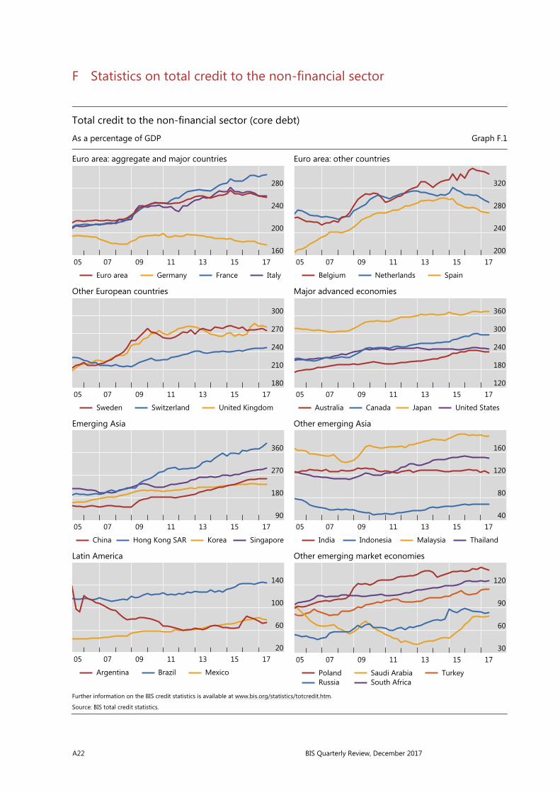
A22 BIS Quarterly Review, December 2017
F Statistics on total credit to the non-financial sector
Total credit to the non-financial sector (core debt)
As a percentage of GDP Graph F.1
Euro area: aggregate and major countries Euro area: other countries
Other European countries Major advanced economies
Emerging Asia Other emerging Asia
Latin America Other emerging market economies
Further information on the BIS credit statistics is available at www.bis.org/statistics/totcredit.htm.
Source: BIS total credit statistics.
280
240
200
16017151311090705
Euro area Germany France Italy
320
280
240
20017151311090705
Belgium Netherlands Spain
300
270
240
210
18017151311090705
Sweden Switzerland United Kingdom
360
300
240
180
12017151311090705
Australia Canada Japan United States
360
270
180
9017151311090705
China Hong Kong SAR Korea Singapore
160
120
80
4017151311090705
India Indonesia Malaysia Thailand
140
100
60
2017151311090705
Argentina Brazil Mexico
120
90
60
3017151311090705
PolandRussia
Saudi ArabiaSouth Africa
Turkey

BIS Quarterly Review,December 2017 A23
Total credit to the private non-financial sector (core debt)
As a percentage of GDP Graph F.2
Euro area: aggregate and major countries Euro area: other countries
Other European countries Major advanced economies
Emerging Asia Other emerging Asia
Latin America Other emerging market economies
Further information on the BIS credit statistics is available at www.bis.org/statistics/totcredit.htm.
Source: BIS total credit statistics.
180
150
120
9017151311090705
Euro area Germany France Italy
225
200
175
15017151311090705
Belgium Netherlands Spain
225
200
175
15017151311090705
Sweden Switzerland United Kingdom
210
180
150
12017151311090705
Australia Canada Japan United States
280
210
140
7017151311090705
China Hong Kong SAR Korea Singapore
120
80
40
017151311090705
India Indonesia Malaysia Thailand
60
40
20
017151311090705
Argentina Brazil Mexico
80
60
40
2017151311090705
PolandRussia
Saudi ArabiaSouth Africa
Turkey

A24 BIS Quarterly Review, December 2017
Bank credit to the private non-financial sector (core debt)
As a percentage of GDP Graph F.3
Euro area: aggregate and major countries Euro area: other countries
Other European countries Major advanced economies
Emerging Asia Other emerging Asia
Latin America Other emerging market economies
Further information on the BIS credit statistics is available at www.bis.org/statistics/totcredit.htm.
Source: BIS total credit statistics.
100
90
80
70
6017151311090705
Euro area Germany France Italy
150
120
90
60
3017151311090705
Belgium Netherlands Spain
160
140
120
100
8017151311090705
Sweden Switzerland United Kingdom
120
90
60
30
017151311090705
Australia Canada Japan United States
200
150
100
5017151311090705
China Hong Kong SAR Korea Singapore
120
90
60
30
017151311090705
India Indonesia Malaysia Thailand
60
45
30
15
017151311090705
Argentina Brazil Mexico
75
60
45
30
1517151311090705
PolandRussia
Saudi ArabiaSouth Africa
Turkey

BIS Quarterly Review,December 2017 A25
Total credit to households (core debt)
As a percentage of GDP Graph F.4
Euro area: aggregate and major countries Euro area: other countries
Other European countries Major advanced economies
Emerging Asia Other emerging Asia
Latin America Other emerging market economies
Further information on the BIS credit statistics is available at www.bis.org/statistics/totcredit.htm.
Source: BIS total credit statistics.
70
60
50
40
3017151311090705
Euro area Germany France Italy
120
100
80
60
4017151311090705
Belgium Netherlands Spain
120
100
80
60
4017151311090705
Sweden Switzerland United Kingdom
120
100
80
60
4017151311090705
Australia Canada Japan United States
80
60
40
20
017151311090705
China Hong Kong SAR Korea Singapore
80
60
40
20
017151311090705
India Indonesia Malaysia Thailand
28
21
14
7
017151311090705
Argentina Brazil Mexico
40
30
20
10
017151311090705
PolandRussia
Saudi ArabiaSouth Africa
Turkey

A26 BIS Quarterly Review, December 2017
Total credit to non-financial corporations (core debt)
As a percentage of GDP Graph F.5
Euro area: aggregate and major countries Euro area: other countries
Other European countries Major advanced economies
Emerging Asia Other emerging Asia
Latin America Other emerging market economies
Further information on the BIS credit statistics is available at www.bis.org/statistics/totcredit.htm.
Source: BIS total credit statistics.
120
100
80
60
4017151311090705
Euro area Germany France Italy
160
140
120
100
8017151311090705
Belgium Netherlands Spain
150
125
100
75
5017151311090705
Sweden Switzerland United Kingdom
120
105
90
75
6017151311090705
Australia Canada Japan United States
240
180
120
60
017151311090705
China Hong Kong SAR Korea Singapore
100
75
50
25
017151311090705
India Indonesia Malaysia Thailand
45
30
15
017151311090705
Argentina Brazil Mexico
60
45
30
1517151311090705
PolandRussia
Saudi ArabiaSouth Africa
Turkey

BIS Quarterly Review,December 2017 A27
Total credit to the government sector at market value (core debt)1
As a percentage of GDP Graph F.6
Euro area: aggregate and major countries Euro area: other countries
Other European countries Major advanced economies
Emerging Asia Other emerging market economies
Further information on the BIS credit statistics is available at www.bis.org/statistics/totcredit.htm. 1 Consolidated data for the general government sector.
Source: BIS total credit statistics.
150
125
100
75
5017151311090705
Euro area Germany France Italy
125
100
75
50
2517151311090705
Belgium Netherlands Spain
150
120
90
60
30
17151311090705
Sweden Switzerland United Kingdom
200
150
100
50
0
17151311090705
Australia Canada Japan United States
55
45
35
25
1517151311090705
Korea
55
45
35
25
1517151311090705
Poland Turkey

A28 BIS Quarterly Review, December 2017
Total credit to the government sector at nominal value (core debt)1
As a percentage of GDP Graph F.7
Euro area: aggregate and major countries Euro area: other countries
Other European countries Major advanced economies
Emerging Asia Other emerging Asia
Latin America Other emerging market economies
Further information on the BIS credit statistics is available at www.bis.org/statistics/totcredit.htm. 1 Consolidated data for the general government sector; central government for Argentina, Indonesia, Malaysia, Mexico, Saudi Arabia and Thailand.
Source: BIS total credit statistics.
125
100
75
5017151311090705
Euro area Germany France Italy
100
75
50
2517151311090705
Belgium Netherlands Spain
90
75
60
45
30
17151311090705
Sweden Switzerland United Kingdom
200
150
100
50
0
17151311090705
Australia Canada Japan United States
100
75
50
25
0
17151311090705
China Hong Kong SAR Singapore
75
60
45
30
15
17151311090705
India Indonesia Malaysia Thailand
100
75
50
25
0
17151311090705
Argentina Brazil Mexico
80
60
40
20
0
17151311090705
PolandRussia
Saudi ArabiaSouth Africa
Turkey
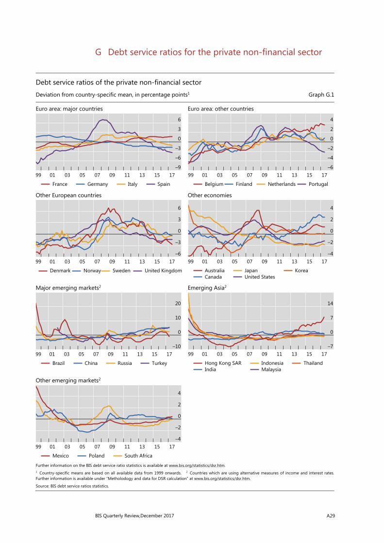
BIS Quarterly Review,December 2017 A29
G Debt service ratios for the private non-financial sector
Debt service ratios of the private non-financial sector
Deviation from country-specific mean, in percentage points1 Graph G.1
Euro area: major countries Euro area: other countries
Other European countries Other economies
Major emerging markets2 Emerging Asia2
Other emerging markets2
Further information on the BIS debt service ratio statistics is available at www.bis.org/statistics/dsr.htm. 1 Country-specific means are based on all available data from 1999 onwards. 2 Countries which are using alternative measures of income and interest rates. Further information is available under “Metholodogy and data for DSR calculation” at www.bis.org/statistics/dsr.htm.
Source: BIS debt service ratios statistics.
6
3
0
–3
–6
–917151311090705030199
France Germany Italy Spain
4
2
0
–2
–4
–617151311090705030199
Belgium Finland Netherlands Portugal
6
3
0
–3
–617151311090705030199
Denmark Norway Sweden United Kingdom
4
2
0
–2
–417151311090705030199
AustraliaCanada
JapanUnited States
Korea
20
10
0
–1017151311090705030199
Brazil China Russia Turkey
14
7
0
–717151311090705030199
Hong Kong SARIndia
IndonesiaMalaysia
Thailand
4
2
0
–2
–417151311090705030199
Mexico Poland South Africa

A30 BIS Quarterly Review, December 2017
Debt service ratios of households
Deviation from country-specific mean, in percentage points1 Graph G.2
Euro area: major countries Euro area: other countries
Other European countries Other economies
Further information on the BIS debt service ratio statistics is available at www.bis.org/statistics/dsr.htm. 1 Country-specific means are based on all available data from 1999 onwards.
Source: BIS debt service ratios statistics.
4
2
0
–2
–417151311090705030199
France Germany Italy Spain
2
0
–2
–4
–617151311090705030199
Belgium Finland Netherlands Portugal
4
2
0
–2
–417151311090705030199
Denmark Norway Sweden United Kingdom
2
0
–2
–4
–617151311090705030199
AustraliaCanada
JapanUnited States
Korea
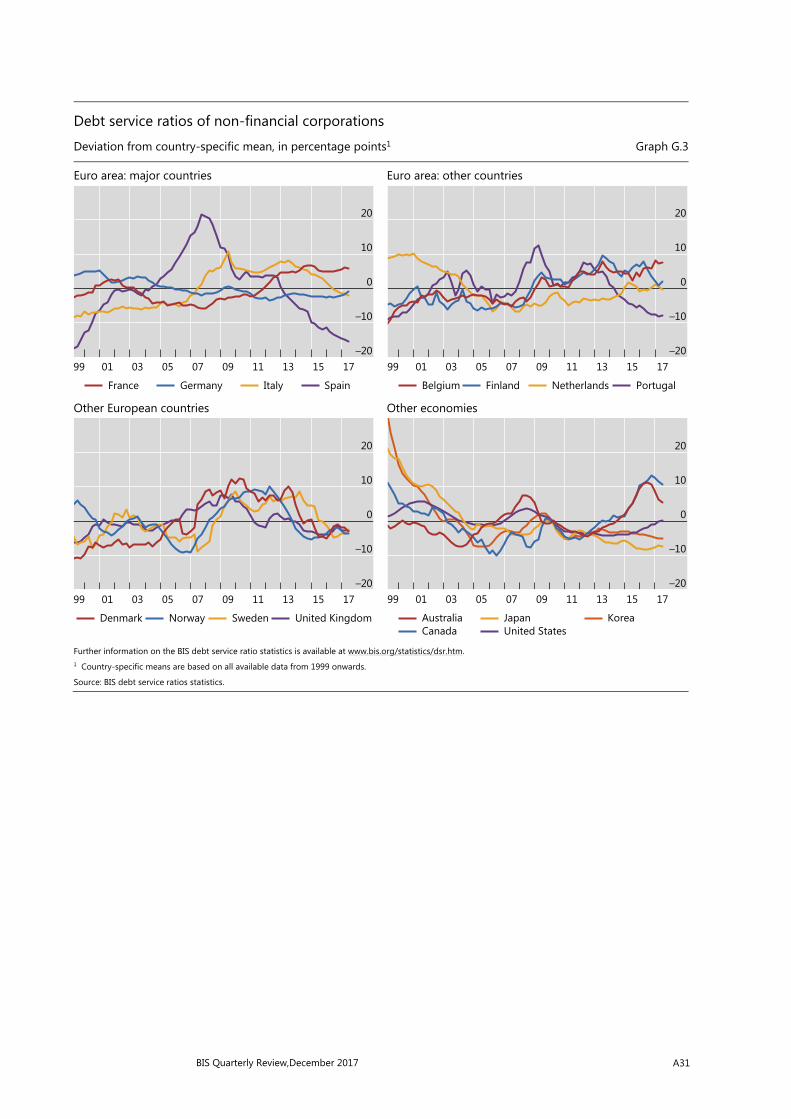
BIS Quarterly Review,December 2017 A31
Debt service ratios of non-financial corporations
Deviation from country-specific mean, in percentage points1 Graph G.3
Euro area: major countries Euro area: other countries
Other European countries Other economies
Further information on the BIS debt service ratio statistics is available at www.bis.org/statistics/dsr.htm. 1 Country-specific means are based on all available data from 1999 onwards.
Source: BIS debt service ratios statistics.
20
10
0
–10
–2017151311090705030199
France Germany Italy Spain
20
10
0
–10
–2017151311090705030199
Belgium Finland Netherlands Portugal
20
10
0
–10
–2017151311090705030199
Denmark Norway Sweden United Kingdom
20
10
0
–10
–2017151311090705030199
AustraliaCanada
JapanUnited States
Korea
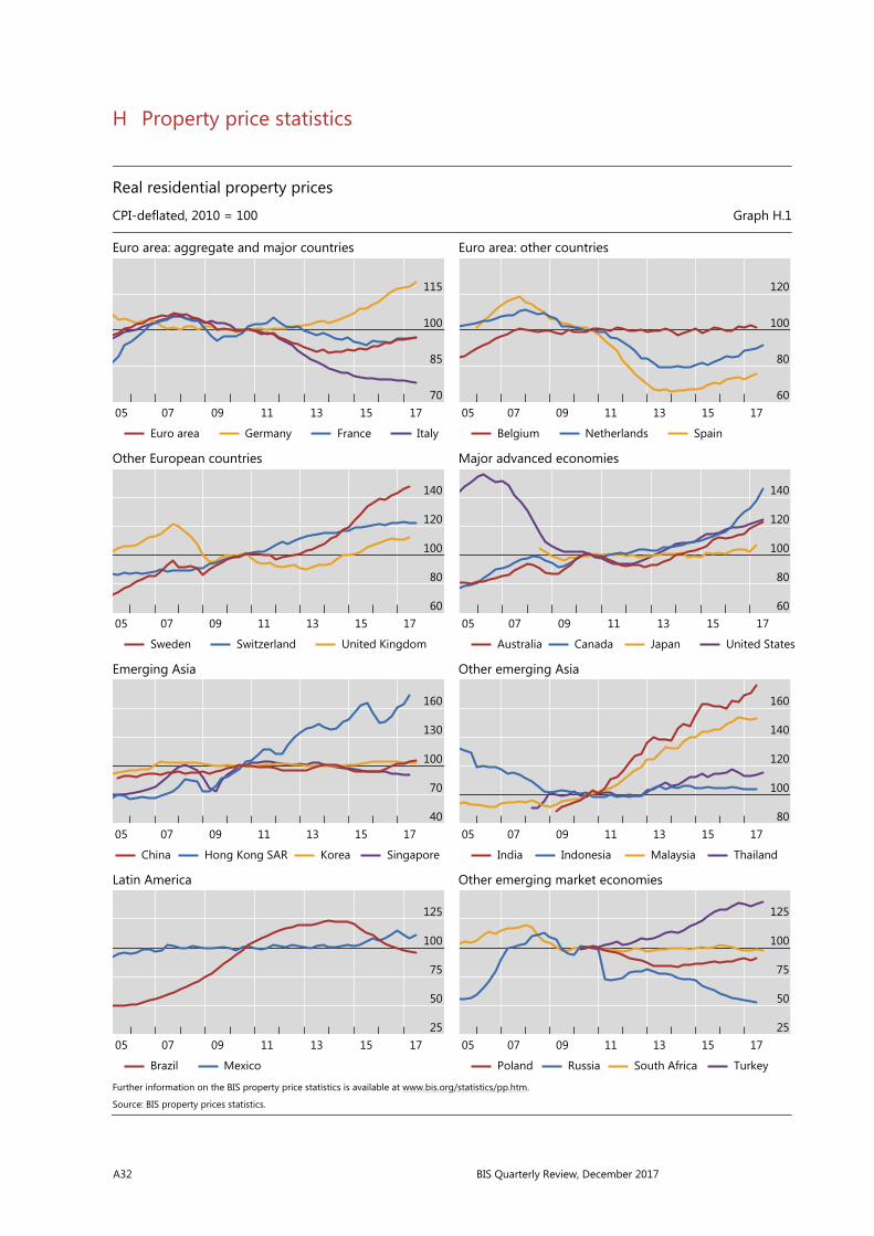
A32 BIS Quarterly Review, December 2017
H Property price statistics
Real residential property prices
CPI-deflated, 2010 = 100 Graph H.1
Euro area: aggregate and major countries Euro area: other countries
Other European countries Major advanced economies
Emerging Asia Other emerging Asia
Latin America Other emerging market economies
Further information on the BIS property price statistics is available at www.bis.org/statistics/pp.htm.
Source: BIS property prices statistics.
115
100
85
7017151311090705
Euro area Germany France Italy
120
100
80
6017151311090705
Belgium Netherlands Spain
140
120
100
80
6017151311090705
Sweden Switzerland United Kingdom
140
120
100
80
6017151311090705
Australia Canada Japan United States
160
130
100
70
4017151311090705
China Hong Kong SAR Korea Singapore
160
140
120
100
8017151311090705
India Indonesia Malaysia Thailand
125
100
75
50
2517151311090705
Brazil Mexico
125
100
75
50
2517151311090705
Poland Russia South Africa Turkey

BIS Quarterly Review,December 2017 A33
I Effective and US dollar exchange rate statistics
Real effective exchange rates CPI-based, 1995–2005 = 1001 Graph I.1
Euro area: aggregate and major countries Euro area: other countries
Other European countries Major advanced economies
Emerging Asia Other emerging Asia
Latin America Other emerging market economies
Further information on the BIS effective exchange rate statistics is available at www.bis.org/statistics/eer.htm. 1 An increase indicates a real-term appreciation of the local currency against a broad basket of currencies.
Source: BIS effective exchange rates statistics.
120
110
100
90
8017151311090705
Euro area Germany France Italy
120
110
100
90
8017151311090705
Belgium Netherlands Spain
120
100
80
6017151311090705
Sweden United Kingdom Switzerland
125
100
75
5017151311090705
Australia Canada Japan United States
125
100
75
5017151311090705
China Hong Kong SAR Korea Singapore
120
100
80
6017151311090705
India Indonesia Malaysia Thailand
125
100
75
50
2517151311090705
Argentina Brazil Mexico
150
125
100
75
5017151311090705
PolandRussia
Saudi ArabiaSouth Africa
Turkey
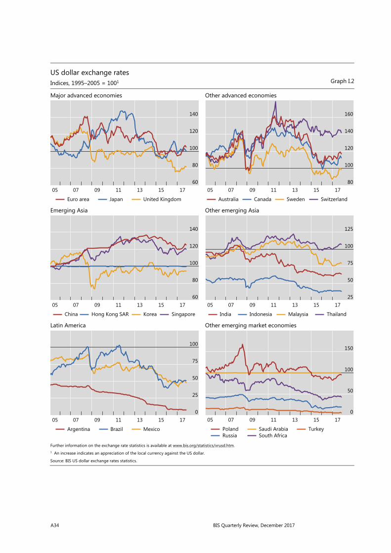
A34 BIS Quarterly Review, December 2017
US dollar exchange rates Indices, 1995–2005 = 1001 Graph I.2
Major advanced economies Other advanced economies
Emerging Asia Other emerging Asia
Latin America Other emerging market economies
Further information on the exchange rate statistics is available at www.bis.org/statistics/xrusd.htm. 1 An increase indicates an appreciation of the local currency against the US dollar.
Source: BIS US dollar exchange rates statistics.
140
120
100
80
6017151311090705
Euro area Japan United Kingdom
160
140
120
100
8017151311090705
Australia Canada Sweden Switzerland
140
120
100
80
6017151311090705
China Hong Kong SAR Korea Singapore
125
100
75
50
2517151311090705
India Indonesia Malaysia Thailand
100
75
50
25
017151311090705
Argentina Brazil Mexico
150
100
50
017151311090705
PolandRussia
Saudi ArabiaSouth Africa
Turkey
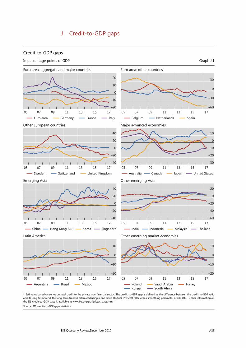
BIS Quarterly Review,December 2017 A35
J Credit-to-GDP gaps
Credit-to-GDP gaps
In percentage points of GDP Graph J.1
Euro area: aggregate and major countries Euro area: other countries
Other European countries Major advanced economies
Emerging Asia Other emerging Asia
Latin America Other emerging market economies
1 Estimates based on series on total credit to the private non-financial sector. The credit-to-GDP gap is defined as the difference between the credit-to-GDP ratio and its long-term trend; the long-term trend is calculated using a one-sided Hodrick-Prescott filter with a smoothing parameter of 400,000. Further information on the BIS credit-to-GDP gaps is available at www.bis.org/statistics/c_gaps.htm.
Source: BIS credit-to-GDP gaps statistics.
20
10
0
–10
–2017151311090705
Euro area Germany France Italy
30
0
–30
–6017151311090705
Belgium Netherlands Spain
40
20
0
–20
–4017151311090705
Sweden Switzerland United Kingdom
10
0
–10
–20
–3017151311090705
Australia Canada Japan United States
40
20
0
–20
–4017151311090705
China Hong Kong SAR Korea Singapore
20
0
–20
–40
–6017151311090705
India Indonesia Malaysia Thailand
10
0
–10
–2017151311090705
Argentina Brazil Mexico
10
0
–10
–2017151311090705
PolandRussia
Saudi ArabiaSouth Africa
Turkey

A36 BIS Quarterly Review, December 2017
K Consumer prices
Consumer prices Year-on-year percentage changes Graph K.1
Euro area: aggregate and major countries Euro area: other countries
Other European countries Major advanced economies
Emerging Asia Other emerging Asia
Latin America Other emerging market economies
Further information on the BIS consumer prices is available at www.bis.org/statistics/cp.htm.
Source: BIS consumer price statistics.
4
2
0
–217151311090705
Euro area Germany France Italy
4
2
0
–217151311090705
Belgium Netherlands Spain
4
2
0
–2
–417151311090705
Sweden United Kingdom Switzerland
4
2
0
–2
–417151311090705
Australia Canada Japan United States
9
6
3
0
–317151311090705
China Hong Kong SAR Korea Singapore
15
10
5
0
–517151311090705
India Indonesia Malaysia Thailand
30
20
10
0
17151311090705
Argentina Brazil Mexico
15
10
5
0
17151311090705
PolandRussia
Saudi ArabiaSouth Africa
Turkey

BIS Quarterly Review,December 2017 A37
L Central bank policy rates
Central bank policy or representative rates Month-end; in per cent Graph L.1
Major advanced economies Other advanced economies
Emerging Asia Other emerging Asia
Latin America Other emerging market economies
Further information on the policy rates is available at www.bis.org/statistics/cbpol.htm.
Source: BIS policy rates statistics.
6
4
2
0
–217151311090705
Euro areaJapan
United KingdomUnited States
6
4
2
0
–217151311090705
Australia Canada Sweden Switzerland
6
4
2
0
–217151311090705
China Hong Kong SAR Korea
12
9
6
3
017151311090705
India Indonesia Malaysia Thailand
30
20
10
017151311090705
Argentina Brazil Mexico
15
10
5
017151311090705
PolandRussia
Saudi ArabiaSouth Africa
Turkey


BIS Quarterly Review, December 2017 B1
Special features in the BIS Quarterly Review
September 2017 FX swaps and forwards: missing global debt? Claudio Borio, Robert McCauley & Patrick McGuire
September 2017 Central bank cryptocurrencies Morten Bech & Rodney Garratt
September 2017 What are the effects of macroprudential policies on macroeconomic performance?
Codruta Boar, Leonardo Gambacorta, Giovanni Lombardo & Luiz Pereira da Silva
September 2017 Green bond finance and certification Torsten Ehlers & Frank Packer
March 2017 Consumption-led expansions Enisse Kharroubi & Emanuel Kohlscheen
March 2017 The new era of expected credit loss provisioning Benjamin Cohen & Gerald Edwards Jr
March 2017 The quest for speed in payments Morten Bech, Yuuki Shimizu and Paul Wong
March 2017 The bond benchmark continues to tip to swaps Lawrence Kreicher, Robert McCauley & Philip Wooldridge
December 2016 Downsized FX markets: causes and implications Michael Moore, Andreas Schrimpf and Vladyslav Sushko
December 2016 The changing shape of interest rate derivatives markets Torsten Ehlers & Egemen Eren
December 2016 Emerging derivatives markets? Christian Upper & Marcos Valli
December 2016 Non-deliverable forwards: impact of currency internationalisation and derivatives reform
Robert McCauley & Chang Shu
December 2016 Does the financial channel of exchange rates offset the trade channel?
Jonathan Kerns & Nikhil Patel


BIS Quarterly Review, December 2017 C1
Recent BIS publications1
BIS Working Papers
CoCo issuance and bank fragility Stefan Avdjiev, Bilyana Bogdanova, Patrick Bolton, Wei Jiang and Anastasia Kartasheva November 2017, No 678
The promise of contingent convertible capital securities (CoCos) as a 'bail-in' solution has been the subject of considerable theoretical analysis and debate, but little is known about their effects in practice. In this paper, we undertake the first comprehensive empirical analysis of bank CoCo issues, a market segment that comprises over 730 instruments totaling $521 billion. Four main findings emerge: 1) The propensity to issue a CoCo is higher for larger and better-capitalized banks; 2) CoCo issues result in statistically significant declines in issuers' CDS spreads, indicating that they generate risk-reduction benefits and lower costs of debt. This is especially true for CoCos that: i) convert into equity, ii) have mechanical triggers, iii) are classified as Additional Tier 1 instruments; 3) CoCos with only discretionary triggers do not have a significant impact on CDS spreads; 4) CoCo issues have no statistically significant impact on stock prices, except for principal write-down CoCos with a high trigger level, which have a positive effect.
Macroeconomic implications of financial imperfections: a survey Stijn Claessens and M Ayhan Kose November 2017, No 677
This paper surveys the theoretical and empirical literature on the macroeconomic implications of financial imperfections. It focuses on two major channels through which financial imperfections can affect macroeconomic outcomes. The first channel, which operates through the demand side of finance and is captured by financial accelerator-type mechanisms, describes how changes in borrowers' balance sheets can affect their access to finance and thereby amplify and propagate economic and financial shocks. The second channel, which is associated with the supply side of finance, emphasises the implications of changes in financial intermediaries' balance sheets for the supply of credit, liquidity and asset prices, and, consequently, for macroeconomic outcomes. These channels have been shown to be important in explaining the linkages between the real economy and the financial sector. That said, many questions remain.
Asset prices and macroeconomic outcomes: a survey Stijn Claessens and M Ayhan Kose November 2017, No 676
This paper surveys the literature on the linkages between asset prices and macroeconomic outcomes. It focuses on three major questions. First, what are the basic theoretical linkages between asset prices and macroeconomic outcomes? Second, what is the empirical evidence supporting these linkages? And third, what are the main challenges to the theoretical and empirical findings? The survey addresses these questions in the context of four major asset price categories: equity prices, house prices, exchange rates and interest rates, with a particular focus on their international dimensions. It also puts into perspective the evolution of the literature on the determinants of asset prices and their linkages with macroeconomic outcomes, and discusses possible future research directions.
1 Requests for publications should be addressed to Bank for International Settlements, Press &
Communications, Centralbahnplatz 2, CH-4002 Basel. These publications are also available on the BIS website (http://www.bis.org/).

C2 BIS Quarterly Review, December 2017
Macroprudential Policies in Peru: The effects of Dynamic Provisioning and Conditional Reserve Requirements Elias Minaya, José Lupú and Miguel Cabello November 2017, No 675
Over the past decade, credit has grown significantly in Peru, a small and partially dollarised economy, and the mounting credit risk attached to foreign currency credit created severe challenges for financial regulators. This paper assesses the effectiveness of two macroprudential measures implemented by regulators: dynamic provisioning, to reduce the procyclicality of credit and conditional reserve requirements, to diminish the degree of dollarisation of the economy. Using credit register data that covers the period of 2004-2014, we find evidence that dynamic provisioning has decelerated the rapid growth of commercial bank lending. Moreover, mortgage dollarisation declined significantly after the implementation of the conditional reserve requirement scheme.
Credit supply responses to reserve requirement: loan-level evidence from macroprudential policy João Barata R B Barroso, Rodrigo Barbone Gonzalez and Bernardus F Nazar Van Doornik November 2017, No 674
This paper estimates the impact of reserve requirements (RR) on credit supply in Brazil, exploring a large loan-level dataset. We use a difference-in-difference strategy, first in a long panel, then in a cross-section. In the first case, we estimate the average effect on credit supply of several changes in RR from 2008 to 2015 using a macroprudential policy index. In the second, we use the bank-specific regulatory change to estimate credit supply responses from (1) a countercyclical easing policy implemented to alleviate a credit crunch in the aftermath of the 2008 global crisis; and (2) from its related tightening. We find evidence of a lending channel where more liquid banks mitigate RR policy. Exploring the two phases of countercyclical policy, we find that the easing impacted the lending channel on average two times more than the tightening. Foreign and small banks mitigate these effects. Finally, banks are prone to lend less to riskier firms.
Loan-to-value policy and housing finance: effects on constrained borrowers Douglas Kiarelly Godoy de Araujo, João Barata R B Barroso and Rodrigo Barbone Gonzalez November 2017, No 673
This paper explores the effects on constrained borrowers of an LTV limit implemented on September 2013 on two major segments of housing finance in Brazil. LTV (hard) limits and related policies entail identification challenges, since constrained individuals are no longer directly observed after policy implementation. In this paper, partially observed treatment status is overcome by the use of an adjusted difference-in-difference method, focusing on the average treatment effect on the treated borrowers (i.e. those that would violate the LTV limit if allowed to do so). We use comprehensive loan-level data on mortgages augmented with a detailed and granular employment register. In the most affected segment, constrained individuals must meet the new LTV limit. These treated borrowers purchase more affordable homes and are less likely to be in arrears 12 months in the future. In the least affected segment, constrained borrowers also end-up meeting the new LTV limit, but the impacts are smaller and we find no significant effects on borrower's housing choice or morose debt.
Capital and currency-based macroprudential policies: an evaluation using credit registry data Horacio A Aguirre and Gastón Repetto November 2017, No 672
We aim to assess the impact of capital- and currency-based macroprudential policy measures on credit growth at the bank-firm level, using credit registry data from Argentina. We examine the impact of the introduction and tightening of a capital buffer and a limit on the foreign currency position of financial institutions on credit growth of firms, estimating fixed effects and difference-in-difference models for the period 2009-2014; we control for macroeconomic, financial institutions and firms' variables, both observable and unobservable. We find that: the capital buffer and the limits on foreign currency positions generally contribute to moderating the credit cycle, both when introduced and when tightened; the

BIS Quarterly Review, December 2017 C3
currency-based measure appears to have a quantitatively more important impact; both measures operate on the extensive and the intensive margins, and have an impact on credit supply. Macroprudential policies also have an effect on ex post credit quality: growth of non-performing loans is reduced after their implementation. In general, credit granted by banks with more capital and assets evidences a higher impact of the introduction of the capital buffer, while this measure also acts more strongly during economic activity expansions.
Capital misallocation and financial development: A sector-level analysis Daniela Marconi and Christian Upper November 2017, No 671
This study investigates how financial development affects capital allocation across industries in a panel of countries at different stages of development (China, India, Mexico, Korea, Japan and the US) over the period 1980-2014. Following the approach proposed by Chari et al (2007) and Aoki (2012), we compute wedges for capital and labour inputs for 26 industrial sectors in the six countries and add them up to economy-wide measures of capital and labour misallocation. We find that more developed financial systems allocate capital investment more efficiently than less developed ones. If financial development is low, faster capital accumulation is associated with a worsening of allocative efficiency. This effect reverses for higher levels of financial development. Sectors with high R&D expenditures or high capital investment benefit most from financial development. These effects are not only statistically significant, they are also large in economic terms.
Policy Rules for Capital Controls Gurnain Kaur Pasricha November 2017, No 670
This paper attempts to borrow the tradition of estimating policy reaction functions in monetary policy literature and apply it to capital controls policy literature. Using a novel weekly dataset on capital controls policy actions in 21 emerging economies over the period 1 January 2001 to 31 December 2015, I examine the competitiveness and macroprudential motivations for capital control policies. I introduce a new proxy for competitiveness motivations: the weighted appreciation of an emerging-market currency against its top five trade competitors. The analysis shows that past emerging-market policy systematically responds to both competitiveness and macroprudential motivations. The choice of instruments is also systematic: policy-makers respond to competitiveness concerns by using both instruments - inflow tightening and outflow easing. They use only inflow tightening in response to macroprudential concerns. I also find evidence that that policy is acyclical to foreign debt but is countercyclical to domestic bank credit to the private non-financial sector. The adoption of explicit financial stability mandates by central banks or the creation of inter-agency financial stability councils increased the weight of macroprudential factors in the use of capital controls policies. Countries with higher exchange rate pass-through to export prices are more responsive to competitiveness concerns.
Credit misallocation during the European financial crisis Fabiano Schivardi, Enrico Sette and Guido Tabellini November 2017, No 669
Do banks with low capital extend excessive credit to weak firms, and does this matter for aggregate efficiency? Using a unique dataset that covers almost all bank-firm relationships in Italy in the period 2004-2013, we find that during the Eurozone financial crisis (i) undercapitalized banks were less likely to cut credit to non-viable firms; (ii) credit misallocation increased the failure rate of healthy firms and reduced the failure rate of non-viable firms and (iii) nevertheless, the adverse effects of credit misallocation on the growth rate of healthier firms were negligible, as were the effects on TFP dispersion. This goes against previous influential findings, which, we argue, face serious identification problems. Thus, while banks with low capital can be an important source of aggregate inefficiency in the long run, their contribution to the severity of the great recession via capital misallocation was modest.

C4 BIS Quarterly Review, December 2017
Financial and real shocks and the effectiveness of monetary and macroprudential policies in Latin American countries Javier Garcia-Cicco, Markus Kirchner, Julio Carrillo, Diego Rodríguez, Fernando Perez, Rocío Gondo, Carlos Montoro and Roberto Chang October 2017, No 668
This work compares the impact of monetary and macroprudential policies on financial and real sectors in four Latin American countries: Chile, Colombia, Mexico and Peru, and explores the commonalities and differences in the reaction to shocks to both the financial and real sector. In order to do that, we estimate a New Keynesian small open economy model with frictions in the domestic financial intermediation sector and a commodity sector for each country. Results suggest that financial shocks are important drivers of output and investment fluctuations in the short run for most countries, but in the long run their contribution is small. Furthermore, we evaluate the ability of macroprudential policies to limit the impact on credit growth and its effect on real variables. In a scenario of tighter financial conditions, monetary policy becomes expansionary due to both lower inflation (given the exchange rate appreciation) and weaker output growth, and macroprudential policies further contribute to restoring credit and output growth. However, in the case of a negative commodity price shock, macroprudential policies are less effective but useful as a complement for the tightening of monetary policy. Higher inflation (due to the exchange rate depreciation) and higher policy rates lead to a contraction in output growth, but macroprudential policies could alleviate this by improving credit conditions.
Modeling Time-Varying Uncertainty of Multiple-Horizon Forecast Errors Todd E Clark, Michael W McCracken and Elmar Mertens October 2017, No 667
We develop uncertainty measures for point forecasts from surveys such as the Survey of Professional Forecasters, Blue Chip, or the Federal Open Market Committee's Summary of Economic Projections. At a given point of time, these surveys provide forecasts for macroeconomic variables at multiple horizons. To track time-varying uncertainty in the associated forecast errors, we derive a multiple-horizon speci cation of stochastic volatility. Compared to constant-variance approaches, our stochastic-volatility model improves the accuracy of uncertainty measures for survey forecasts.
Bank capital allocation under multiple constraints Tirupam Goel, Ulf Lewrick and Nikola Tarashev October 2017, No 666
Banks allocate capital across business units while facing multiple constraints that may bind contemporaneously or only in future states. When risks rise or risk management strengthens, a bank reallocates capital to the more efficient unit. This unit would have generated higher constraint- and risk-adjusted returns while satisfying a tightened constraint at the old capital allocation. Calibrated to US data, our model reveals that, when credit or market risk increases, market-making attracts capital and lending shrinks. Leverage constraints affect banks only when measured risks are low. At low credit risk, tighter leverage constraints may reduce market-making but support lending.
Interest rates and house prices in the United States and around the world Gregory Sutton, Dubravko Mihaljek and Agnė Subelytė October 2017, No 665
This paper estimates the response of house prices to changes in short- and long-term interest rates in 47 advanced and emerging market economies. We use data that statistical authorities selected as their best house price series, covering almost half a century of quarterly observations for the United States and over 1,000 annual observations for the rest of the sample. We find a surprisingly important role for short-term interest rates as a driver of house prices, especially outside the United States. Our interpretation is that this reflects the importance of the bank lending channel of monetary policy in house price fluctuations, especially in countries where securitisation of home mortgages is less prevalent. In addition, we document substantial inertia in house prices and find that changes in interest rates and other determinants affect house

BIS Quarterly Review, December 2017 C5
prices gradually rather than on impact. This suggests that modest cuts in policy rates are not likely to rapidly fuel house price increases. Finally, we find that US interest rates seem to affect house prices outside the United States.
Is the price right? Swing pricing and investor redemptions Ulf Lewrick and Jochen Schanz October 2017, No 664
How effective are available policy tools in managing liquidity risks in the mutual fund industry? We assess one such tool - swing pricing - which allows funds to adjust their settlement price in response to large net flows. Our empirical analysis exploits the fact that swing pricing is available to Luxembourg funds, but not yet to U.S. funds. We show that swing pricing dampens outflows in reaction to weak fund performance, but has a limited effect during stress episodes. Furthermore, swing pricing supports fund returns, while raising accounting volatility, and may lead to lower cash buffers.
Liquidity risk in markets with trading frictions: What can swing pricing achieve? Ulf Lewrick and Jochen Schanz October 2017, No 663
Open-end mutual funds expose themselves to liquidity risk by granting their investors the right to daily redemptions at the fund's net asset value. We assess how swing pricing can dampen such risks by allowing the fund to settle investor orders at a price below the fund's net asset value. This reduces investors' incentive to redeem shares and mitigates the risk of large destabilising outflows.Optimal swing pricing balances this risk with the benefit of providing liquidity to cash-constrained investors. We derive bounds, depending on trading costs and the share of liquidity-constrained investors, within which a fund chooses to swing the settlement price. We also show how the optimal settlement price responds to unanticipated shocks. Finally, we discuss whether swing pricing can help mitigate the risk of self-fulfilling runs on funds.
The real effects of relationship lending Ryan Niladri Banerjee, Leonardo Gambacorta and Enrico Sette September 2017, No 662
This paper studies the real consequences of relationship lending on firm activity in Italy following Lehman Brothers' default shock and Europe's sovereign debt crisis. We use a large data set that merges the comprehensive Italian Credit and Firm Registers. We find that following Lehman's default, banks offered more favourable continuation lending terms to firms with which they had stronger relationships. Such favourable conditions enabled firms to maintain higher levels of investment and employment. The insulation effects of tighter bank-firm relationships was still present during the European sovereign debt crisis, especially for firms tied to well capitalised banks.
Basel Committee on Banking Supervision
Identification and management of step-in risk October 2017
As part of the G20's initiative to strengthen the oversight and regulation of the shadow banking system, the Basel Committee on Banking Supervision's Guidelines on identification and management of step-in risk aim to mitigate the systemic risks stemming from potential financial distress in shadow banking entities spilling over to banks.
The guidelines build upon two public consultations carried out by the Committee in December 2015 and March 2017. They introduce a flexible and tailored approach, where measures to mitigate significant step-in risk rely on a supervisory process that is supported by proportionate reporting. In particular:
Banks define the scope of entities to be evaluated for potential step-in risk, based on the relationship of these entities with the bank

C6 BIS Quarterly Review, December 2017
Banks identify entities that are immaterial or subject to collective rebuttals and exclude them from the initial set of entities to be evaluated
Banks assess all remaining entities against the step-in risk indicators provided in the guidelines, including potential mitigants
For entities where step-in risk is identified, banks estimate the potential impact on liquidity and capital positions and determine the appropriate internal risk management action
Banks report their self-assessment of step-in risk to their supervisor
After reviewing the bank's self-assessment analysis, where necessary supported by an analysis of the bank's policies and procedures, the supervisor should decide whether there is a need for an additional supervisory response. To that extent, the guidelines do not prescribe any automatic Pillar 1 liquidity or capital charge, but rather rely on the application of existing prudential measures available to mitigate significant step-in risk.
The guidelines are expected to be implemented in member jurisdictions by 2020.
Thirteenth progress report on adoption of the Basel regulatory framework October 2017
This updated Progress report on adoption of the Basel regulatory framework provides a high-level view of Basel Committee members' progress in adopting Basel III standards as of end-September 2017.
The report focuses on the status of adoption of all the Basel III standards (which will become effective by 2019) to ensure that the Basel standards are transformed into national law or regulation according to the internationally agreed timeframes. The report is based on information provided by individual members as part of the Committee's Regulatory Consistency Assessment Programme (RCAP). The report includes the status of adoption of the Basel III risk-based capital standards, the liquidity coverage ratio (LCR), the net stable funding ratio (NSFR), the standards for global and domestic systemically important banks (SIBs), the leverage ratio, the large exposure framework, the interest rate risk in the banking book (IRRBB), and the disclosure requirements.
In addition to periodically reporting on the status of adoption, all Committee members undergo an assessment of the consistency of their domestic rules with the Basel standards.
Regulatory Consistency Assessment Programme (RCAP) - Assessment of Basel III LCR regulations - Switzerland October 2017
This report presents the findings of an RCAP Assessment Team on the adoption of the Basel Liquidity Coverage Ratio (LCR) in Switzerland and its consistency with the minimum requirements of the Basel III framework. The assessment is based on the Swiss LCR rules of the Liquidity Ordinance, supplemented by circulars issued by Swiss Financial Market Supervisory Authority (FINMA).
The assessment focuses on the consistency and completeness of the Swiss LCR rules with the Basel minimum requirements. Issues relating to prudential outcomes, the liquidity position of individual banks or the effectiveness of the FINMA’s supervisory effectiveness were not in the scope of this RCAP. The assessment relied upon the Swiss regulations and other information and explanations provided by the Swiss authorities and ultimately reflects the expert view of the Assessment Team on the documents and data reviewed. Where deviations from the Basel framework were identified, they were evaluated for their current and potential impact on the reported LCR for a sample of internationally active banks in Switzerland. The materiality assessment relied upon the data, information and computations provided by FINMA. Some findings were evaluated on a qualitative basis in instances where appropriate quantitative data were not available. The overall assessment outcome was then based on the materiality of findings (in both quantitative and qualitative terms) and expert judgment. The Assessment Team followed the methodology and guidance provided in the RCAP Handbook for Jurisdictional Assessments.

BIS Quarterly Review, December 2017 C7
Regulatory Consistency Assessment Programme (RCAP) - Assessment of Basel III LCR regulations - Canada October 2017
This report presents the findings of an RCAP assessment on the domestic adoption of the Basel Liquidity Coverage Ratio (LCR) standard in Canada and its consistency with the minimum requirements of the Basel III framework. The assessment focuses on the rules applied to Canadian banks that are internationally active and of significance to domestic financial stability, in particular the consistency and completeness of the Canadian regulations with the Basel minimum requirements. It is based on the Canadian regulations in force on 30 June 2017. Issues relating to prudential outcomes, the liquidity position of individual banks or the supervisory effectiveness of the Canadian authorities were not in the scope of this RCAP assessment.
The Where domestic regulations and provisions were found to be non-compliant with the Basel framework, those deviations were evaluated for their current and potential impact (or non-impact) on the reported LCRs of a sample of Canadian banks. The assessment outcome was based on the materiality of findings and expert judgment.
The report has three sections and a set of annexes: (i) an executive summary with a statement from the Canadian authorities on the assessment outcome; (ii) the context, scope and methodology, together with the main assessment findings; and (iii) details of the deviations and their materiality along with other assessment-related observations.
Regulatory Consistency Assessment Programme (RCAP) - Assessment of Basel III LCR regulations - Brazil October 2017
This report presents the findings of an RCAP Assessment Team on the domestic adoption of the Basel Liquidity Coverage Ratio (LCR) standard in Brazil and its consistency with the minimum requirements of the Basel III framework. The assessment focuses on the Brazilian banks that are internationally active and of significance to domestic financial stability.
The focus of the assessment was on the consistency and completeness of the Brazilian regulations with the Basel minimum requirements, based on the regulations in force on 31 July 2017. Issues relating to prudential outcomes, the liquidity position of individual banks, or the Brazilian authorities’ supervisory effectiveness were not in the scope of this RCAP assessment. The assessment reflects the expert view of the Assessment Team on the documents, data and explanations provided by the Brazilian authorities.
Regulatory Consistency Assessment Programme (RCAP) - Assessment of Basel III LCR regulations - Australia October 2017
This report presents the findings of an RCAP Assessment Team on the domestic adoption of the Basel Liquidity Coverage Ratio (LCR) in Australia and its consistency with the minimum requirements of the Basel III framework. The assessment is based on the Australian LCR rules of the Authorised Deposit-taking Institutions (ADI) Prudential Standards (APS), supplemented by the ADI Reporting Standards (ARS) and ADI Prudential Practice Guide (APG).
The focus of the assessment was on the consistency and completeness of the Australian LCR rules with the Basel minimum requirements. Issues relating to prudential outcomes, the liquidity position of individual banks or the effectiveness of APRA’s supervisory effectiveness were not in the scope of this RCAP assessment. The assessment relied upon data, information and materiality computations provided by APRA and was based on Australian regulations in force as of 30 June 2017. Where deviations from the Basel III framework were identified, they were evaluated for their current and potential impact on the reported LCR for a sample of internationally active banks in Australia. Some findings were evaluated on a qualitative basis in instances where appropriate quantitative data were not available. The overall assessment outcome was then based on the materiality of findings (in both quantitative and qualitative terms) and ultimately reflects the expert view of the Assessment Team. The Assessment Team

C8 BIS Quarterly Review, December 2017
followed the methodology and guidance provided in the RCAP Handbook for Jurisdictional Assessments.2
Risk weight for Asian Infrastructure Investment Bank October 2017
The Basel Committee on Banking Supervision has agreed that supervisors may allow banks to apply a 0% risk weight to claims on the Asian Infrastructure Investment Bank (AIIB) in accordance with paragraph 59 of the document International Convergence of Capital Measurement and Capital Standards: A revised Framework - Comprehensive Version, June 2006. AIIB will be included in the list of multilateral development banks as set out in footnote 24 of the document.
Basel III definition of capital - Frequently asked questions October 2017
The Basel Committee periodically reviews frequently asked questions (FAQs) on its standards and publishes answers to these together with technical elaboration of the rules text and interpretative guidance where necessary. These aim to promote consistent global implementation of Basel III.
The FAQs published in this document correspond to the definition of capital sections of the Basel III standards and the 13 January 2011 press release on the loss absorbency of capital at the point of non-viability. These FAQs are in addition to those previously published in July 2011, October 2011 and December 2011. They are grouped according to the relevant paragraphs of the rules text. FAQs that have been added since the publication of the third version of this document are listed at the start of the document and marked in italics.
Basel III Monitoring Report September 2017
This report presents the results of the Basel Committee's latest Basel III monitoring exercise based on data as of 31 December 2016. The Committee established a rigorous reporting process to regularly review the implications of the Basel III standards for banks, and it has published the results of previous exercises since 2012. For the first time, the report provides not only global averages but also a regional breakdown for many key metrics.
Data have been provided for a total of 200 banks, comprising 105 large internationally active banks. These "Group 1 banks" are defined as internationally active banks that have Tier 1 capital of more than €3 billion, and include all 30 banks that have been designated as global systemically important banks (G-SIBs). The Basel Committee's sample also includes 95 "Group 2 banks" (ie banks that have Tier 1 capital of less than €3 billion or are not internationally active).
The Basel III minimum capital requirements are expected to be fully phased-in by 1 January 2019 (while certain capital instruments could still be recognised for regulatory capital purposes until end-2021). On a fully phased-in basis, data as of 31 December 2016 show that all banks in the sample meet both the Basel III risk-based capital minimum Common Equity Tier 1 (CET1) requirement of 4.5% and the target level CET1 requirement of 7.0% (plus any surcharges for G-SIBs, as applicable). Between 30 June and 31 December 2016, Group 1 banks continued to reduce their capital shortfalls relative to the higher Tier 1 and total capital target levels; in particular, the Tier 2 capital shortfall has decreased from €3.4 billion to €0.3 billion. As a point of reference, the sum of after-tax profits prior to distributions across the same sample of Group 1 banks for the six-month period ending 31 December 2016 was €239.5 billion. In addition, applying the 2022 minimum requirements for Total Loss-Absorbing Capacity (TLAC), 12 of the G-SIBs in the sample have a combined incremental TLAC shortfall of €116.4 billion as at the end of December 2016, compared with €318.2 billion at the end of June 2016.
2 See www.bis.org/bcbs/publ/d361.pdf.

BIS Quarterly Review, December 2017 C9
The monitoring reports also collect bank data on Basel III's liquidity requirements. Basel III's Liquidity Coverage Ratio (LCR) was set at 60% in 2015, increased to 70% in 2016 and will continue to rise in equal annual steps to reach 100% in 2019. The weighted average LCR for the Group 1 bank sample was 131% on 31 December 2016, up from 126% six months earlier. For Group 2 banks, the weighted average LCR was 159%, slightly up from 158% six months earlier. Of the banks in the LCR sample, 91% of the Group 1 banks (including all G-SIBs) and 96% of the Group 2 banks reported an LCR that met or exceeded 100%, while all Group 1 and Group 2 banks reported an LCR at or above the 70% minimum requirement that was in place for 2016.
Basel III also includes a longer-term structural liquidity standard - the Net Stable Funding Ratio (NSFR). The weighted average NSFR for the Group 1 bank sample was 116%, while for Group 2 banks the average NSFR was 114%. As of December 2016, 94% of the Group 1 banks (including all G-SIBs) and 88% of the Group 2 banks in the NSFR sample reported a ratio that met or exceeded 100%, while 100% of the Group 1 banks and 96% of the Group 2 banks reported an NSFR at or above 90%.
Committee on Payments and Market Infrastructures
Statistics on payment, clearing and settlement systems in the CPMI countries - Figures for 2016 (preliminary version) October 2017 No 171
This is an annual publication that provides data on payments and payment, clearing and settlement systems in the CPMI countries.
This version of the statistical update contains data for 2016 and earlier years. There are detailed tables for each individual country as well as a number of comparative tables.
A final version will be published in December 2017.
Discussion note - Reducing the risk of wholesale payments fraud related to endpoint security - consultative document September 2017 No 170 The Committee on Payments and Market Infrastructures (CPMI) has published a consultative document, Discussion note - Reducing the risk of wholesale payments fraud related to endpoint security.
This strategy aims to help focus industry efforts to tackle the increasing threat of wholesale payments fraud related to endpoint security. The strategy sets out seven elements designed to address all areas relevant to preventing, detecting, responding to and communicating about wholesale payments fraud. It stresses the importance of understanding the full range of risks and calls upon all relevant public and private sector stakeholders to take a holistic and coordinated approach.
The CPMI is now seeking input from relevant stakeholders. After the consultation, it plans to develop guidance on each of the seven elements to help operators and participants of payment systems and messaging networks as well as their respective supervisors, regulators and overseers improve endpoint security. Proposed guidance will be developed by early 2018.
Harmonisation of the Unique Product Identifier - Technical Guidance September 2017 No 169
G20 Leaders agreed in 2009 that all over-the-counter (OTC) derivatives contracts should be reported to trade repositories (TRs) as part of their commitment to reform OTC derivatives markets in order to improve transparency, mitigate systemic risk and protect against market abuse. Aggregation of the data reported across TRs is necessary to help ensure that authorities are able to obtain a comprehensive view of the OTC derivatives market and activity.

C10 BIS Quarterly Review, December 2017
Following the 2014 FSB Feasibility study on approaches to aggregate OTC derivatives data, the FSB asked the CPMI and IOSCO to develop global guidance on the harmonisation of data elements reported to TRs and important for the aggregation of data by authorities, including Unique Transaction Identifiers (UTIs) and Unique Product Identifiers (UPIs).
This report is one part of the CPMI-IOSCO Harmonisation Group's response to its mandate. It focuses on the harmonised global UPI, whose purpose is to uniquely identify each OTC derivative product involved in a transaction that an authority requires, or may require in the future, to be reported to a TR. The guidance is global in scale, takes account of relevant international technical standards where available and is jurisdiction-agnostic, thus enabling the consistent global aggregation of OTC derivatives transaction data.
The CPMI and IOSCO issued a Technical Guidance on Harmonisation of the Unique Transaction Identifier in February 2017.
Speeches
Can central banks talk too much?
Speech by Mr Hyun Song Shin, Economic Adviser and Head of Research of the BIS, at the ECB conference on "Communications challenges for policy effectiveness, accountability and reputation", Frankfurt, 14 November 2017.
Is it possible for central banks to talk too much? Central banks learn from market prices, and influence market prices to steer the economy. However, the signal value of market prices can become impaired when market participants place too much weight on central bank pronouncements and actions. One concrete example of the confounding of market signals is the behaviour of market-implied inflation expectations based on the inflation swaps market, where swap rates have begun to move in lockstep with nominal yields. Such instances remind us that communication is a two-way street that involves listening as well as talking. Listening with greater self-awareness of the central bank's outsized role in financial markets would give central banks space to take a more detached position and make better decisions.
Recent regulatory developments and remaining challenges
Presentation by Mr Fernando Restoy, Chairman, Financial Stability Institute, Bank for International Settlements, at the CIV Meeting of Central Bank Governors of the Center for Latin American Monetary Studies (CEMLA), Washington DC, 12 October 2017.
The presentation provides an overview of the achievements to date of the post-crisis regulatory reforms and the ongoing work of the different standard-setting bodies. It highlights some specific challenges for financial sector authorities, including the ex post impact assessment of regulatory reforms; the problem of non-performing loans in several jurisdictions; the application of proportionality in regulation; the emergence of fintech; the implementation of resolution reforms; and other priority areas such as cyber-risk, shadow banking and correspondent banking.
Leverage in the small and in the large
Panel remarks by Mr Hyun Song Shin, Economic Adviser and Head of Research of the BIS, at the IMF conference on "Systemic Risk and Macroprudential Stress Testing", Washington DC, 10 October 2017.
Leverage in the small refers to the leverage of individual institutions, while leverage in the large refers to the leverage of the financial system as a whole. These two notions correspond to two directions in gauging systemic risk. One is to drill down to detailed micro evidence of how financial institutions are intertwined and delve into the complex web of interconnections. The other direction is to "drill up", to the macro, and indeed global, aggregates. Of the two, drilling up is often more informative, as it delivers the all-important time dimension of systemic risk - how it builds up over time and how it unwinds. I argue for

BIS Quarterly Review, December 2017 C11
two propositions. First, mitigating complexity is mostly about taming leverage in the small. The motto is: if you take care of leverage in the small, complexity will take care of itself. Second, lest we fall into complacency, taming complexity is not enough to ward off systemic risk. Systemic risk is mostly about leverage in the large. Addressing systemic risk entails taking a macro and global perspective. Here, the motto is: take a global approach to macroprudential frameworks
Avoiding "regulatory wars" using international coordination of macroprudential policies
Article by Mr Luiz Awazu Pereira da Silva, Deputy General Manager of the BIS, and Mr Michael Chui, Senior Economist, based on panel remarks at the Seminar on Financial Volatility and Foreign Exchange Intervention: Challenges for Central Banks, jointly organised by the Inter-American Development Bank and the Central Reserve Bank of Peru, Cusco, 25-26 July 2017.
Financial spillovers and spillbacks have increased significantly in magnitude since the Global Financial Crisis posing a threat to financial stability. Using macroprudential policies following systematic countercyclical rules reduces volatility and contributes to financial stability, growth and investment. However, a multiplication of non-systematic, local macroprudential policies, and capital flow management measures including more aggressive capital controls, might result in a "regulatory war" and reduce global welfare. Instead, other avenues could be explored, as demonstrated by the adaptability of the policy frameworks used by emerging market economies. They have constantly evolved as a result of lessons learned from crises and that should include the Global Financial Crisis. This evolution is part of a learning curve that uses past crisis experiences, policymaking and research to prevent vulnerabilities from developing into full-blown future crises. These remarks are meant to show how this process occurs, its importance for global stability and a last but much needed "new lesson". Global financial stability needs international coordination on macroprudential policies between major emerging market economies (those that represent a large combined share of the global economy) and the major advanced economies.
Is there a risk of snapback in long-dated yields?
Panel remarks by Mr Hyun Song Shin, Economic Adviser and Head of Research of the BIS, at the Second ECB Annual Research Conference, Frankfurt, 25 September 2017.
Long-term interest rates have stayed low in the face of monetary policy normalisation, but experience has taught us that the bond market can change course quite abruptly. Long rates overreact relative to the benchmark where long rates are the average of expected future short rates. As prices are the outcomes of the interaction of many actors, the exact mechanism behind the overreaction varies over time and across markets, but we can sometimes shed light on what is going on without being able to predict when big market moves will happen. I provide a glimpse of the ultra-long segment of the euro area sovereign bond market through the lens of the insurance sector. The holding of ultra-long bonds by German insurance firms has quadrupled since 2008. In turn, yield-chasing may affect market dynamics to lower long-term rates, sparking even greater demand for long-dated bonds. To an outside observer, it would appear as if market participants' preferences were changing with market prices themselves. Low rates beget low rates through higher value placed on long-dated bonds, and high rates beget high rates due to lower value placed on long-dated bonds.
Through the looking glass
Lecture by Mr Claudio Borio, Head of the Monetary and Economic Department of the BIS, at the OMFIF City Lecture, London, 22 September 2017.
Why has inflation been so stubbornly subdued despite so little excess capacity? And why have real (inflation-adjusted) interest rates declined so much for so long? The lecture argues that these two seemingly independent developments are, in fact, intimately linked. Prevailing paradigms may underestimate how long-lasting the impact of real factors, such as globalisation and, increasingly, technology, may be on inflation; and, conversely, they may underestimate how long-lasting the impact of monetary policy may be on real interest rates.

C12 BIS Quarterly Review, December 2017
If these hypotheses are correct, they could have first-order implications for the future of monetary policy.
Challenges for regulators and supervisors after the post-crisis reforms
Opening address by Mr Jaime Caruana, General Manager of the BIS, at the FSI Conference on "Supervisory policy implementation in the current macro-financial environment - 'a cross-sectoral journey'", Basel, 18 September 2017.
The emphasis on enhancing resilience for the whole system - not just individual institutions - is critical. It also implies a very broad-based endeavour. During the past nine years, major financial reforms have taken place in multiple areas.
In the crisis prevention domain, a number of new standards were developed to increase the resilience of financial institutions and market infrastructures, to make financial transactions safer and to reduce the scope for key entities to generate systemic risks. In the crisis management domain, authorities have developed ways to make the resolution of unviable institutions more orderly in future, ideally without involving government finances - in contrast to what happened in many countries during the crisis.
On this occasion, I will refrain from listing the whole catalogue of reforms and their implementation status. Should there be any need to assess the breadth and depth of these reforms, I believe you are familiar with the multiple and detailed progress reports produced by the individual standard setters and the Financial Stability Board (FSB).1 For an overview, I recommend the latest FSB annual report on implementation and effects of the G20 financial regulatory reforms.2
Although there are still a few important pending issues, it is fair to recognise that a huge amount of work has taken place over the past nine years. These efforts have contributed to making the financial system more resilient and better equipped to facilitate sustainable economic growth. Also worth highlighting is that this progress is largely the consequence of an impressive, possibly unprecedented, international cooperation effort, involving authorities from jurisdictions around the world.
Designing the reforms is only the first step. After developing a comprehensive reform package that affects almost all aspects of the financial system, there is still the need to complete what is pending and concentrate efforts on proper implementation and monitoring effects.
Completing the elements that are pending is, of course, essential. Basel III comes to mind - and I expect that it will soon be finalised. Stabilising the regulatory framework will help the financial sector adjust and adapt to these changes.
At this point in the regulatory cycle, one of the best contributions that the international regulatory community could make in support of financial stability is to promote the comprehensive, consistent and timely implementation of the reforms.
Before turning to implementation, my main topic today, let me add a couple of thoughts that we at the BIS believe to be important to bear in mind.
First, it would be a mistake to declare victory too soon. The world economy is still subject to risks and vulnerabilities, most notably those relating to the generalised increase in indebtedness and the rich valuations of assets. As we know from experience, debt is an extremely powerful mechanism that can amplify the destabilising impact of adverse shocks.
Second, financial stability is a very elusive, multifaceted objective. Its pursuit requires the contribution of other policies. Monetary, fiscal and structural reform policies also need to contribute to limiting financial stability risks both at the national level and globally. I don't think that prudential policies, not even together with macroprudential ones, can do the job alone.
Against this background, let me turn to my main topic.
We all agree that proper implementation is essential to reaping the full benefits of the global regulatory reforms. It is crucial to ensure consistency among the different segments of

BIS Quarterly Review, December 2017 C13
the regulated financial sector. It is also vital to promote a level playing field both within and across jurisdictions.
Policy implementation: three dimensions
In talking about implementation, I would like to adopt a relatively wide definition, under which good policy implementation covers three different but related dimensions.
The first relates to adopting the new standards into national regulation in a proper, consistent and timely way. The second is about assessing whether these standards, once implemented, are achieving their objectives. The third is about putting in place supervisory frameworks that help maximise the benefits of the new standards.
Adopting new standards in a proper, consistent and timely way
First and foremost, implementation requires the proper adoption of the new regulatory standards. As documented in the progress reports of the various standard setters and the FSB, significant progress has been made in implementing the new standards in all domains. This general progress, however, is uneven.
The various standard setters have identified some areas where more expeditious implementation is desirable in some jurisdictions. This is the case, for example, for the standards relating to counterparty credit risk in the banking sphere. This is also the case for the standards relating to margin requirements for non-centrally cleared derivatives, even though implementation has taken place in the major financial centres.
The FSB, for its part, has identified in its latest review of post-crisis reforms that substantial work remains to be done before an adequate implementation of resolution regimes can take place in a number of jurisdictions. This is particularly the case regarding resolution powers. The key missing powers are those that enable bail-in and those that allow for a temporary stay on the exercise of early termination rights.3
In other words, the adoption of new rules is still very much a work in progress.
In talking about implementation, we often emphasise the need for consistency. However, consistency does not necessarily require uniform application of standards to all entities and in all jurisdictions. For instance, as you know, the Basel Committee standards are minimum standards. There is scope for supervisors to ask for more than the minimum if necessary. And these standards are in principle meant to apply to large international banks. We need to be sensitive to the compliance costs.
Following the principle of proportionality, it may be appropriate to apply simpler standards to banks with simpler business models - as long as this does not result in less stringent requirements for these institutions. Indeed, ever since its Market Risk Amendment in 1996, the Basel Committee has envisaged the use of both standardised and advanced methods for determining capital charges, with the former applying to less complex businesses. In fact, this simpler, standardised approach is associated with higher capital requirements. And a number of jurisdictions currently apply specific rules to purely domestic banks.
Yet, when applying the principle of proportionality, we should give due consideration to the potential consequences that may result from heterogeneous regulatory requirements. For example, we should consider what impact such heterogeneity might have on the resilience of individual institutions, or on the domestic competitive environment.
Assessing whether standards, once implemented, achieve their objectives
The second dimension of implementation relates to assessing the reforms' impact once we gain some experience with operating under the new rules. Given the wide scope of the reforms, spanning virtually all segments of financial activity, it is necessary to assess their combined impact on the financial system and on the real economy.
Since the early stages of designing the current reforms, there have been significant efforts to assess their potential impacts. As these reforms are being implemented, more valuable information is becoming available to assess whether the new rules are working as

C14 BIS Quarterly Review, December 2017
intended and whether they generate adverse unintended effects. These can include the excessive shift of risks towards less regulated areas,4 the reduced liquidity in some securities markets or the retrenched provision of correspondent banking services to some countries. Such assessments no doubt require a comprehensive and inter-sectoral approach to grasp the whole range of effects that the new standards could generate.
This comprehensive analysis should build on the extensive impact assessments conducted by each standard setter. For instance, the Basel Committee began conducting impact assessments more than a decade ago, when finalising Basel II. Ever since, it has developed and refined its methodologies, conducting increasingly elaborate assessments of its standards.5
The next logical step is to systematically conduct and generalise these types of assessments. Indeed, the FSB, in cooperation with the relevant standard setters, has recently launched a methodological framework6 for the evaluation of the post-crisis reforms so as to analyse their overall effects and to compare these with their objectives.
In this context, two elements seem to be critical to me:
The first is about the need for fact-driven analysis as well as data availability and quality. To assess the impact of reforms, we will need sufficient practical experience with the reforms and long enough series of robust data. The usefulness of these assessments for policy recommendations will depend on the extent to which they can identify and measure the effects of regulation. Gaining experience and gathering good data will take time. Good collaboration with the private sector will thus be crucial. It may also require an additional effort by private sector stakeholders to ensure the quality of their IT systems and the information they can provide.
The second critical point about assessment methodology - and perhaps the biggest challenge in this regard - is the need to establish some kind of reference point, some kind of measurable benchmark that helps to capture the social benefits and costs of the reforms. This will help determine whether the actual outcomes are satisfactory and sufficient to meet the reforms' intended objectives.
In any case, this collaborative effort at the FSB, when combined with all of the ongoing impact assessments conducted by the individual standard setters, will no doubt help address concerns about potential imperfections in the different standards.
At the same time, we should be careful to avoid the impression that there will be frequent adjustments to the regulatory standards. Otherwise, we would be contradicting our objective to achieve soon a sufficiently stable and predictable regulatory environment. This stability is also critical for an evidence-based assessment of the impact of the reforms over time.
Putting in place supervisory frameworks that maximise the benefits of new standards
The third dimension of policy implementation is to have supervisory frameworks that help support and maximise the positive effects of the regulatory reforms on the proper functioning of the financial system. This is a broad topic that includes resources, powers, methodologies, cooperation, etc. Let me focus on a few specific observations.
First, the crisis has confirmed the need for supervisors to take a more comprehensive approach to address the build-up of vulnerabilities at financial institutions. Accordingly, they are now increasing their efforts to directly assess asset quality, proper classifications, valuations and provisions. At the same time, supervisors are combining this traditional focus with greater attention to corporate culture and governance, including the framework for risk appetite and the compensation system. All these elements must be part of their comprehensive efforts to identify vulnerabilities. Importantly, authorities are now complementing the traditional microprudential focus of their supervisory programmes with a macro perspective. This allows them to better assess system-wide risk concentrations, the build-up of financial imbalances and procyclical effects.

BIS Quarterly Review, December 2017 C15
Supervisory priorities and practices are also becoming more forward-looking. Over the last few years, national supervisors have increasingly combined the analysis of financial statements, supervisory reporting and on-site inspections with stress testing exercises to assess banks' resilience under different risk scenarios. Supervisors are also assessing and challenging the sustainability of banks' business models in order to anticipate difficulties.
More cooperation across authorities when conducting stress tests could enhance the analysis. This would help, for instance, to improve the assessment of cross-border spillover effects. It would also help to take these effects into consideration in a more consistent manner across jurisdictions.
Another key lesson reconfirmed by the crisis is the need for supervisory intervention to be more proactive. This generally means earlier and perhaps more forceful interventions that address problems well before the situation deteriorates to the point of non-viability. Proactive supervisory interventions have long been a known challenge because they involve delicate trade-offs. In particular, they rely not only on early identification of problems, but also on the exercise of just enough supervisory discretion and supervisory powers to solve the problems at stake. Doing too much would risk arbitrary intervention. Doing too little would risk complacency.
Last but not least, technological innovations are facilitating the emergence of new players in the market for financial services. That in turn is forcing supervised institutions to change and to adapt their business models. These changes can increase the efficiency of the industry. In some jurisdictions, they may also encourage financial inclusion. But at the same time, innovations and new players also mean that the nature of the risks affecting the financial system is evolving. All these developments require specific policy attention by both conduct of business supervisors and prudential supervisors. The Basel Committee's current public consultation on the implications of fintech for the financial sector is one recent case in point.7
Concluding remarks
Let me conclude. I started my intervention by highlighting the magnitude of the post-crisis regulatory reforms and their progress. These reforms will help the orderly functioning of the financial sector. They will promote systemic stability and, therefore, sustainable growth. That being said, there is no room for complacency. We certainly need to work more, especially - but not exclusively - on policy implementation. Avoiding watering down what we have achieved so far, completing Basel III and implementing the reforms in a consistent and timely manner are top priorities.
I want to reiterate, however, that the task of maintaining financial stability goes beyond ensuring effective regulation and supervision. The vulnerabilities in the financial system often have multiple causes. It is therefore important to recognise the interactions across policy domains in order to deliver an adequate combination of policy actions - a combination that helps to meet all objectives effectively.
This can only be achieved through the work of the international regulatory community. Without the dedicated spirit of cooperation across national authorities, the substantial strengthening of regulations governing the functioning of the financial system would not have been possible. We should certainly maintain this attitude and level of commitment in order to deal effectively with the challenges that lie ahead of us.
One key aspect of this cooperation is the exchanges of practices and experiences among regulators and supervisors to help ensure that sound policy approaches are adopted worldwide. I believe that the Financial Stability Institute can support the standard setters in this regard and should continue to play a key role in promoting the adoption of good policy practices across jurisdictions. This work goes well beyond the dissemination of standards. It also includes, as the FSI is now doing, facilitating information-sharing and providing analysis that helps financial sector authorities identify the appropriate policy approaches. I believe that this conference organised by the FSI fits very well with the objective to promote reflection and cooperation, across countries and sectors, in the field of policy implementation.

C16 BIS Quarterly Review, December 2017
International arrangements for a resilient global economy
Keynote speech by Mr Jaime Caruana, General Manager of the BIS, at the conference on "The uncertain future of global economic integration", jointly organised by the Central Bank of Iceland and the Reinventing Bretton Woods Committee, Reykjavik, 14 September 2017.
The existing international monetary and financial system leaves much room for improvement. In financial regulation, extensive international cooperation coexists with domestic mandates. Yet, when it comes to monetary policy, domestic mandates are broadly considered to rule out cooperation. This is so even though these policies' international spillovers through global financial markets are widely recognised to be powerful.
It is true that, if policymakers could better manage their own domestic financial cycles, they would already constrain excesses and reduce spillovers. But keeping one's own house in order is not enough. Policymakers should also give more weight to how domestic policies interact at a global level. A necessary step is to reach a common understanding of how various spillovers and spillbacks work. Developing analytical frameworks that better capture these effects is a start. Going one step further, more international cooperation on monetary policy could also provide backing for financial stability. Monetary policymakers should take further practical steps to complement their domestic analysis with a more global perspective.emphasis on enhancing resilience for the whole system - not just individual institutions - is critical. It also implies a very broad-based endeavour.
Early intervention regimes: the balance between rules vs discretion
Speech by Mr Fernando Restoy, Chairman, Financial Stability Institute, Bank for International Settlements, at the FSI-IADI Meeting on early supervisory intervention, resolution and deposit insurance, Basel, Switzerland, 12 September 2017.
This meeting takes place at an interesting juncture - almost exactly 10 years after the financial crisis, which is widely acknowledged to have started when BNP Paribas stopped redemptions on three of its money market funds due to its inability to value their subprime mortgage exposures. This was followed shortly thereafter by an old-fashioned bank run at the UK mortgage lender Northern Rock. The failure of Northern Rock turned out to be the first of many high-profile bank failures in a number of countries, with additional collapses averted only by extraordinary government bailouts.
Fortunately, the post-crisis regulatory reforms have led to a more resilient financial system where financial crises are, we hope, less frequent and less costly. Yet, the world economy still faces a number of risks - including the protracted low interest rate environment, excessive indebtedness, potential for regulatory arbitrage and the overcapacity of the banking sector in some jurisdictions - which, collectively, may contribute to new episodes of financial instability. In this context, I cannot emphasise enough the critical role that all the safety net authorities that are gathered around this table can play in fostering a stable financial system.
I will touch upon the evolution, nature and use of early intervention frameworks including their role during the financial crisis. I will also provide a few thoughts about the age-old debate on the appropriate balance between rules and discretion as it relates to early intervention frameworks.