BIS Quarterly Review - Bank for International … Quarterly Review, December 2012 iii BIS Quarterly...

BIS Quarterly ReviewDecember 2012

International banking and financial market developments

This publication is available on the BIS website (www.bis.org).

© Bank for International Settlements 2012. All rights reserved. Brief excerpts may be reproduced or translated provided the source is stated.

ISSN 1683-0121 (print)

ISSN 1683-013X (online)

BIS Quarterly Review Monetary and Economic Department Editorial Committee:

Claudio Borio Dietrich Domanski Christian Upper Stephen Cecchetti Philip Turner General queries concerning this commentary should be addressed to Christian Upper(tel +41 61 280 8416, e-mail: [email protected]), queries concerning specific parts to the authors,whose details appear at the head of each section, and queries concerning the statistics toPhilip Wooldridge (tel +41 61 280 8006, e-mail: [email protected]).

BIS Quarterly Review, December 2012 iii

BIS Quarterly Review

December 2012

International banking and financial market developments

Policy measures and reduced short-term risks buoyed markets ............................................. 1 Asset prices rose despite a weakening economic outlook ........................................... 1 Looser monetary policies supported asset prices ........................................................... 2 Policy easing by major central banks did not lead to emerging market currency appreciation ............................................................................................................. 5 Asset prices were also supported by a reduction in some major downside risks ........................................................................................................................... 6 Conclusion .................................................................................................................................. 10

Highlights of the BIS international statistics .................................................................................... 11 The international banking market in the second quarter of 2012 ........................... 12 Box 1: Shifting credit patterns in emerging Asia ............................................................ 17 Box 2: A reallocation of external positions in the BIS locational banking statistics ...................................................................................................................... 19 The OTC derivatives market in the first half of 2012 ................................................... 19 Box 3: The importance of reference rates ......................................................................... 21

Special features

Natural catastrophes and global reinsurance – exploring the linkages .............................. 23 Sebastian von Dahlen and Goetz von Peter

Physical damage and financial losses ............................................................................... 24 Risk transfer ............................................................................................................................... 26 Peak risks and the reinsurance market ............................................................................. 28 Linkages with financial markets .......................................................................................... 31 Conclusion .................................................................................................................................. 34

The euro area crisis and cross-border bank lending to emerging markets ......................... 37 Stefan Avdjiev, Zsolt Kuti and Előd Takáts

Data .............................................................................................................................................. 38 Regression analysis .................................................................................................................. 39 Decomposition analysis ......................................................................................................... 41 Discussion ................................................................................................................................... 44 Conclusion .................................................................................................................................. 46

On the liquidity coverage ratio and monetary policy implementation ................................... 49 Morten Bech and Todd Keister

A primer on the liquidity coverage ratio .......................................................................... 50 Box 1: Computing the LCR .................................................................................................... 51 Interbank loans, central bank borrowing and the LCR ................................................ 52 Monetary policy implementation and the LCR ............................................................... 53 Box 2: Unconventional monetary policies and the LCR ............................................... 59 Conclusions ................................................................................................................................ 60

Enhancements to the BIS debt securities statistics ........................................................................ 63 Branimir Gruić and Philip Wooldridge

Conceptual challenges ........................................................................................................... 63

iv BIS Quarterly Review, December 2012t

Distinguishing international from domestic issues ....................................................... 66 Box 1: Governing law and the Greek debt restructuring ............................................. 67 Revisions implemented in December 2012 ..................................................................... 68 Box 2: Identifying the market of issue ............................................................................... 70 Future enhancements ............................................................................................................. 74

Statistical Annex .............................................................................................................................. A1

Special features in the BIS Quarterly Review ...................................................... B1

List of recent BIS publications ............................................................................................ B2

Notations used in this Review e estimated

lhs, rhs left-hand scale, right-hand scale

billion thousand million

… not available

. not applicable

– nil or negligible

$ US dollar unless specified otherwise

Differences in totals are due to rounding.

The term “country” as used in this publication also covers territorial entities that are

not states as understood by international law and practice but for which data are

separately and independently maintained.

BIS Quarterly Review, December 2012 1

Policy measures and reduced short-term risks buoyed markets1

In the three months to early December, forecasters cut their projections for global economic growth, yet the prices of most growth-sensitive assets rose. These assets benefited from further loosening of monetary policies and perceptions that some major near-term downside risks to the world economy had diminished. In particular, asset valuations reacted positively to new policy measures aimed at tackling the euro area crisis. They were also supported by news suggesting that a sharp and prolonged fall in Chinese economic growth was less likely. However, downside risks remained. Uncertainty about fiscal policy in the United States, which was on course to tighten substantially in the near term, encouraged cash hoarding and weighed on the prices of assets most vulnerable to budget cuts.

Asset prices rose despite a weakening economic outlook

The prices of most risky assets increased between early September and early December. In the advanced economies, yields on both investment grade and sub-investment grade corporate bonds fell to their lowest levels since before the 2008 financial crisis. The same was true of yields on emerging market bonds, whether issued by sovereigns or corporates, or denominated in local or international currencies. And yields on bonds backed by mortgages and other collateral fell to their lowest levels ever. Meanwhile, equity prices mostly rose during the early part of the period, although they fell back somewhat later on.

Unusually, equity and fixed income gains coincided with a weakening of the global economic outlook. Forecasters cut their projections for 2012 and 2013 global economic growth. Without any significant offsetting upward revisions, they substantially reduced their forecasts for Greece, Italy and Spain in Europe, as well as for Brazil, China and India in the emerging world. In the past, falling growth forecasts have usually been associated with rising expected default rates and higher bond yields. But this time, bond yields fell (Graph 1). Similarly, most equity prices ended the period a little above their starting levels, despite weakening corporate

1 This article was prepared by the BIS Monetary and Economic Department. Questions about the

article can be addressed to Masazumi Hattori ([email protected]) and Nicholas Vause ([email protected]). Questions about data and graphs should be addressed to Magdalena Erdem ([email protected]) and Agne Subelyte ([email protected]).

2 BIS Quarterly Review, December 2012

earnings expectations (Graph 2). Earnings expectations for US companies in the S&P 500 Index dropped particularly sharply following a decline in reported earnings – the first in 11 quarters – and as an unusually high proportion of firms warned that future profits could fall short of analysts’ forecasts.

Looser monetary policies supported asset prices

Market participants attributed a significant part of the rally in asset prices to further loosening by central banks, notably the Federal Reserve. On 13 September, the Fed announced that it would immediately begin expanding its balance sheet through monthly purchases of $40 billion worth of mortgage-backed securities. In contrast to previous rounds of asset buying, US policymakers left the size of the programme open-ended, stating that it would continue until the labour market outlook had substantially improved. At the same time, the Fed pushed its forward guidance several months further into the future, saying that it expected to maintain its policy rate at exceptionally low levels until at least mid-2015, even if the US economic recovery had strengthened by then. The Bank of Japan also extended its asset purchasing programme, both in September and October, raising purchases of Japanese government securities and other assets planned before the end of 2013 by ¥21 trillion. Meanwhile, policy rates were cut in Australia, Brazil, Colombia, the Czech Republic, Hungary, Israel, Korea, the Philippines, Sweden and Thailand.

Bond yields and economic growth forecasts

In per cent Graph 1

Investment grade corporate bonds Emerging market corporate bonds Collateralised bonds

Bond yields are yields on Bank of America Merrill Lynch global bond indices. The collateralised index comprises bonds backed by residential mortgages, commercial mortgages, credit card receivables and other assets. Growth forecasts are approximate annualised three-year-ahead forecasts constructed from projections for the current and three subsequent calendar years.

1 For advanced economies. 2 For emerging markets.

Sources: IMF, World Economic Outlook; Datastream; BIS calculations.

2

3

4

5

6

7

3.0

2.5

2.0

1.5

1.0

0.5

2009 2010 2011 2012

Bond yields (lhs)Growth forecast (rhs)1

3

6

9

12

15

18

7.0

6.5

6.0

5.5

5.0

4.5

2009 2010 2011 2012


1

2

3

4

5

6

3.0

2.5

2.0

1.5

1.0

0.5

2009 2010 2011 2012



The Fed’s measures had significant, if short-lived, effects on US financial markets. Most directly, they compressed yields on mortgage-backed securities, which led to reductions in mortgage rates (Graph 3, left-hand panel). As the gap between these two metrics widened, US bank equity prices increased relative to the equity market as a whole. In addition, the Federal Reserve’s new commitment to potentially unlimited balance sheet expansion boosted both market-based indicators of expected inflation and the prices of precious metals used as inflation

Reaction to news of third round of Federal Reserve asset purchases Graph 3

US MBS yields and mortgage rates Per cent

US inflation expectations1

Per cent

Precious metal prices Dollars per troy ounce

The vertical lines indicate 12 September 2012, the date of last closing prices before the news about Federal Reserve asset purchases.

1 Over a five-year horizon. 2 Average rate on new 30-year fixed rate mortgages according to Bankrate.com. 3 Yield on Barclays Capital index of 30-year mortgage-backed securities (MBS) issued by the Federal National Mortgage Association. 4 Difference between yields on conventional and inflation-linked US Treasury bonds.

Sources: Bloomberg; Datastream.

Equity prices and earnings1

Per share, as percentages of December 2010 prices Graph 2

United States Euro area Emerging markets

1 Prices of equities in the respective Morgan Stanley Capital International indices and average 12-month-ahead forecasts of their earnings.

Source: Datastream.

1.5

2.0

2.5

3.0

3.5

4.0

2012

Mortgage rate2

MBS yield3

1.5

1.7

1.9

2.1

2.3

2.5

2012

Break-even rate4

Inflation swap rate

1,300

1,400

1,500

1,600

1,700

1,800

2012

GoldPlatinum

85

95

105

115

7

8

9

10

2011 2012

Price (lhs) Earnings (rhs)

70

82

94

106

8

9

10

11

2011 2012


75

85

95

105

8

9

10

11

2011 2012



hedges (Graph 3, centre and right-hand panels). With this rise in expected inflation, the US dollar depreciated slightly. Within a few weeks, however, both expected inflation and the value of the dollar returned to the levels seen before the 13 September announcement, possibly because incoming economic data suggested less monetary easing than originally expected.

More broadly, further quantitative stimulus by the major central banks appeared to nudge investors into taking on more risk. In particular, developed market corporate bond funds and emerging market government and corporate bond funds each attracted net inflows (Graph 4).

With investors’ demand for risky assets increasing, bond issuers were able to place more debt than in previous months. This included the sale of some relatively risky types of bond. For example, non-financial corporate bond issuance rose to and remained near its year-to-date peak in September, October and November, with disproportionate increases in sub-investment grade issuance. Also during these three months, emerging market bond issuance outpaced that of the previous year, with placements of corporate bonds rising by more than those of government bonds. And, over the same period, European subordinated bond issuance was distinctly stronger than earlier in the year, not only for financial borrowers, who brought forward some planned 2013 issuance owing to forthcoming regulatory changes, but also for non-financial borrowers.

Bond inflows and major central bank policies

In trillions of US dollars Graph 4

Developed market corporate bonds Emerging market bonds

1 Change over three months in the sum of asset holdings purchased via reserve creation by the Bank of England, the Bank of Japan and the Federal Reserve, and via the ECB’s outstanding longer-term refinancing operations. 2 Net flows over three months into managed bond funds.

Sources: ECB; Bank of Japan; Datastream; EPFR; BIS calculations.

–0.6

–0.3

0.0

0.3

0.6

0.9

1.2

–30

–15

0

15

30

45

60

2009 2010 2011 2012

Change in policy support1Lhs:

Portfolio inflows2Rhs:

–0.6

–0.3

0.0

0.3

0.6

0.9

1.2

–8

–4

0

4

8

12

16

2009 2010 2011 2012

Change in policy support1Lhs:

Portfolio inflows2Rhs:


Policy easing by major central banks did not lead to emerging market currency appreciation

Easier monetary policies in advanced economies raised expectations that capital would flow into emerging market economies, causing their currencies to appreciate. When this happened in November 2010 and June 2011, the US dollar fell by more than 5%. Yet this time the US dollar appreciated in the three months from the beginning of September, both against a number of individual emerging market currencies and on a trade-weighted basis (Graph 5, left-hand panel).

Softer growth prospects in emerging markets partly explain why their currencies and capital flows reacted differently to monetary easing in advanced economies. They also put downward pressure on commodity prices (Graph 5, centre panel).

Several emerging market economies used policy measures in an attempt to stop their currencies from appreciating during the period. The Brazilian central bank intervened in foreign exchange markets, and currency traders gained the impression that other central banks in Latin America and East Asia were also in action. In addition, the Czech central bank said that it might consider intervention, depending on how its currency moved. In Korea, the authorities launched an investigation into compliance with restrictions on banks’ foreign exchange positions that would gain from an appreciation of the local currency. Moreover, they tightened limits on banks’ exposure to currency derivatives. All these measures were generally associated with more stable currency values, as evidenced by option implied volatilities (Graph 5, right-hand panel).

Exchange rates and commodity prices Graph 5

US dollar effective exchange rate1, 2 1 January 2010 = 100

Commodity price indices3 1 January 2010 = 100

Emerging markets FX volatility 4 Per cent

1 Geometric weighted average of 60 bilateral nominal exchange rates, with weights based on trade in 2008–10. 2 The vertical lines indicate the start of the Federal Reserve’s second (3 November 2010) and third (13 September 2012) rounds of asset purchases. 3 S&P Goldman Sachs commodity indices. 4 Index of three-month at-the-money option implied volatilities, weighted by market turnover.

Sources: Bloomberg; Datastream; JP Morgan Chase.

90

95

100

105

2010 2011 201275

100

125

150

2010 2011 2012

AgricultureEnergy

Industrial metals

4

8

12

16

2010 2011 2012


Asset prices were also supported by a reduction in some major downside risks

Asset prices also received support during the period from a perceived reduction in some major downside risks to the world economy. In particular, the prospect of a near-term worsening of the euro area crisis appeared to decline following new policy announcements. Also, the risk of a sharp and prolonged fall in Chinese growth seemed to recede after better than expected October economic data were released. However, the risk of an abrupt tightening of US fiscal policy from the beginning of 2013 lingered and even increased, according to some commentators, after federal elections again delivered a balance of political power vulnerable to stalemates.

Changes in the prices of options insuring against sharp declines in equity prices supported the perceived evolution of these risks (Graph 6). The cost of insuring against falls of 20% or more in the EURO STOXX 50 Index, a proxy for a sharp economic crisis in the euro area, fell in the three months from the beginning of September, although the price of protection against smaller price declines dropped by a similar amount. The cost of insurance against large falls in the Hang Seng Index, which might occur if Chinese economic growth were to slow sharply, also declined. The price of protection against smaller price drops fell by a lesser amount. By contrast, there was some increase in the cost of insuring against a fall of 20% or more in the S&P 500 Index, which might accompany an abrupt tightening of US fiscal policy. This rise slightly outpaced the cost of insuring against smaller price declines.

In the euro area, the ECB’s plans to buy government bonds substantially boosted debt markets and underpinned financial markets more broadly. After ECB President Mario Draghi had alluded to these moves in a speech in London on

Cost of insurance against falls in equity price indices1

Implied volatilities, in per cent Graph 6

EURO STOXX 50 Index Hang Seng Index S&P 500 Index

1 Premiums for insurance against falls in equity price indices over three months relative to three-month forward prices, quoted as the implied volatilities that map to these premiums via the Black-Scholes option pricing formula. Higher implied volatilities correspond to higher premiums.

Source: Bloomberg.

10

20

30

40

2012

Fall>0% Fall>10% Fall>20%

10

20

30

40

2012


10

20

30

40

2012



26 July, the Governing Council provided details on 6 September. The ECB would buy bonds issued by euro area governments with residual maturities of one to three years, with the intention of accepting equal status to other creditors, conditional on those governments first agreeing to follow an economic adjustment programme. Yields on bonds of financially strained governments in the region subsequently fell, having already declined significantly since Mr Draghi’s speech, especially at purchase-eligible maturities (Graph 7).

However, Spanish bond yields soon rebounded. This coincided with upward revisions to 2011 and anticipated 2012 budget deficits, clarification that European funds would not be available to finance legacy bank support programmes and a push for independence by the president of Catalonia. In contrast, Italian bond yields remained at much lower levels and in October the government issued a record amount of debt for a single European offering.

Asset prices rose particularly strongly in Greece, where the government eventually received further loan disbursements from its IMF/EU programme. These were due in September, but Greece had slipped behind some of the programme’s economic targets. The government subsequently negotiated an adjusted programme, which included lower and later payments on Greece’s official debt, transfer to Athens of profits on the Eurosystem’s holdings of Greek government bonds and plans for a private sector debt buyback. According to press reports, many hedge funds bought Greek bonds in anticipation of such an outcome. This helped to drive yields lower in the three months to early December (Graph 7, right-hand panel). The Athens Stock Exchange equity price index rose by almost one third over the same period.

Capital flows also seemed to reflect the view that the euro crisis was less likely to intensify. With investors perceiving a reduced risk of currency

Euro area government bond yields

In per cent Graph 7

Spain Italy Greece

The vertical lines indicate 25 July and 5 September, which respectively provided the last closing yields before ECB President Draghi said that his institution "stands ready to do whatever it takes to save the euro" and the ECB detailed its plans for Outright Monetary Transactions.

Source: Bloomberg.

1

2

3

4

5

6

7

2012

Two-year Ten-year

1

2

3

4

5

6

7

2012

Two-year Ten-year

15

18

21

24

27

30

33

2012

Ten-year


redenomination,2 portfolio investments flowed into Spain and Italy on a net basis in September. At the same time, outflows of deposits and other funding from banks in these countries slowed or levelled off (Graph 8, left-hand and centre panels). Separate data show that deposits at these banks also held up in October. Some of the net capital inflows to Spain and Italy probably came from Germany, as the Bundesbank saw a reduction in its claims on the ECB that were generated by net payments from other euro area countries. Conversely, the Spanish and Italian central banks’ liabilities to the ECB generated by net payments to other euro area countries registered a decrease. These changes ran counter to the trend of the previous year or so (Graph 8, right-hand panel).

Despite this renewed support for the financially strained countries in the euro area, yields on bonds issued by the financially more robust governments were essentially unchanged. Yields on two-year bonds issued by France, Germany and the Netherlands remained close to zero, while yields on their 10-year debt also hovered at historically very low levels. Moody’s downgrading of France from AAA had little effect on these yields.

Financial markets also drew support from news suggesting that a sharp and prolonged slowdown in Chinese economic growth seemed less likely. Fears of a “hard landing” in China were allayed, in particular, by rebounds in industrial production and export growth during October as well as a survey of purchasing managers. This reduced perceived default risk for assets vulnerable to a severe

2 This was suggested, for example, by reductions in spreads between yields on several euro-

denominated bonds issued under international law by Italian government-owned companies and bonds with similar maturities issued by the Italian government under domestic law (see the box on page 70). It was also implied by the prices of intrade.com betting contracts that would pay off if any euro area country announced its intention to exit the euro by a specific date.

Cross-border capital flows and TARGET2 balances of selected euro area countries1

In billions of euros Graph 8

Spain Italy TARGET2 balances1

1 Cumulative net inflows since the start of EMU, and net claims of the national central banks on the ECB that reflect cumulative net purchases of goods and assets from domestic residents settled via the TARGET2 real-time gross settlement system. 2 All capital flows in the financial account of the balance of payments other than direct, portfolio and derivatives investments, excluding those of the central bank. These are largely deposits, loans and repos.

Sources: Deutsche Bundesbank; Bank of Italy; Bank of Spain; Datastream; BIS calculations.

0

120

240

360

480

2009 2010 2011 2012

Portfolio investmentBanking flows2

0

60

120

180

240

2009 2010 2011 2012

Portfolio investmentBanking flows2

–600

–300

0

300

600

2009 2010 2011 2012

GermanyItalySpain


economic slowdown, such as bank loans. Reflecting this, Chinese bank equity prices outperformed non-bank equity prices in the three months to early December.

Although perceptions of major downside risks may have diminished, the effects of weakening economic growth in China nevertheless spread to other emerging markets, notably in Asia. Here, exchange rate movements in 2012 had already highlighted the importance of China to investors in several economies in the region. In particular, the exchange rates of economies highly dependent on exporting to China have moved almost in step, suggesting that they are driven largely by news from China, while those of less dependent economies have moved more idiosyncratically (Graph 9, left-hand and centre panels). Moreover, in the three months from the beginning of September, equity price indices in the more China-dependent Asian emerging market economies underperformed those of the less China-dependent ones. Meanwhile, non-Asian equity price indices appeared to be less driven by China news (Graph 9, right-hand panel).

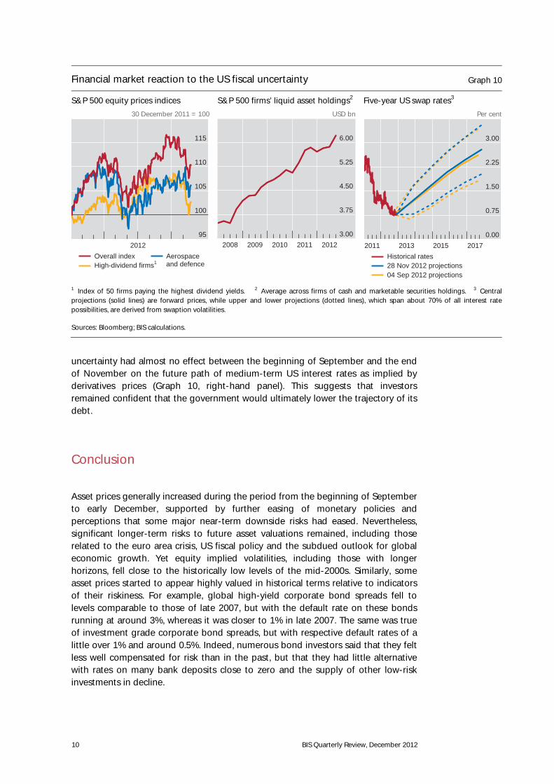
However, not all near-term economic risks diminished, notably in the United States. Here, the government remained on course to cut its budget deficit by around 4% of GDP from the beginning of 2013, which most economists agreed would push the economy into recession. Uncertainty about whether and how this fiscal drag would be mitigated weighed on the prices of certain equities. In particular, prices of stocks with high dividend yields and from the defence sector fell relative to the broader US market. Such stocks are particularly vulnerable to higher dividend taxes and spending cuts, respectively (Graph 10, left-hand panel). Fiscal uncertainty also prompted US companies to keep more liquidity on hand in assets such as bank deposits and marketable securities (Graph 10, centre panel). This put further downward pressure on the yields of those assets. However, this near-term

Asian emerging market exchange rates and equity price indices Graph 9

High China dependence FX rates1, 2 2 January 2012=100

Low China dependence FX rates1, 3 2 January 2012=100

Returns on equity price indices Per cent

AR = Argentina, BR = Brazil, CL = Chile, CO = Colombia, CZ = Czech Republic, HU = Hungary, ID = Indonesia, IN = India, KR = Korea, MX = Mexico, MY = Malaysia, PE = Peru, PH = Philippines, PL = Poland, RU = Russia, SG = Singapore, TH = Thailand, TW = Chinese Taipei, TR = Turkey, ZA = South Africa.

1 US dollars per unit of local currency; an increase indicates an appreciation against the US dollar. 2 Countries with ratios of exports to China to GDP in 2011 above 10%. 3 Countries with ratios of exports to China to GDP in 2011 below 10%. 4 In US dollar terms between end-August and early December 2012.

Sources: IMF, Direction of Trade Statistics, World Economic Outlook; Bloomberg; Datastream.

90

95

100

105

Q1 12 Q2 12 Q3 12 Q4 12

Chinese TaipeiKorea

MalaysiaSingapore

90

95

100

105

Q1 12 Q2 12 Q3 12 Q4 12

IndiaIndonesia

PhilippinesThailand

AR

BRCL

COMX PE

CZ

HU

PL

RUZA

TR

TW

IN

IDKR

MY

PH

SG

TH

–10

–5

0

5

10

0 5 10 15 20

Ret

urns

on

equi

ty p

rice

indi

ces4

Ratio of exports to China to GDP in 2011

Asian emerging marketsOther emerging markets


uncertainty had almost no effect between the beginning of September and the end of November on the future path of medium-term US interest rates as implied by derivatives prices (Graph 10, right-hand panel). This suggests that investors remained confident that the government would ultimately lower the trajectory of its debt.

Conclusion

Asset prices generally increased during the period from the beginning of September to early December, supported by further easing of monetary policies and perceptions that some major near-term downside risks had eased. Nevertheless, significant longer-term risks to future asset valuations remained, including those related to the euro area crisis, US fiscal policy and the subdued outlook for global economic growth. Yet equity implied volatilities, including those with longer horizons, fell close to the historically low levels of the mid-2000s. Similarly, some asset prices started to appear highly valued in historical terms relative to indicators of their riskiness. For example, global high-yield corporate bond spreads fell to levels comparable to those of late 2007, but with the default rate on these bonds running at around 3%, whereas it was closer to 1% in late 2007. The same was true of investment grade corporate bond spreads, but with respective default rates of a little over 1% and around 0.5%. Indeed, numerous bond investors said that they felt less well compensated for risk than in the past, but that they had little alternative with rates on many bank deposits close to zero and the supply of other low-risk investments in decline.

Financial market reaction to the US fiscal uncertainty Graph 10

S&P 500 equity prices indices 30 December 2011 = 100

S&P 500 firms’ liquid asset holdings2

USD bn

Five-year US swap rates3 Per cent

1 Index of 50 firms paying the highest dividend yields. 2 Average across firms of cash and marketable securities holdings. 3 Centralprojections (solid lines) are forward prices, while upper and lower projections (dotted lines), which span about 70% of all interest rate possibilities, are derived from swaption volatilities.

Sources: Bloomberg; BIS calculations.

95

100

105

110

115

2012

Overall indexHigh-dividend firms1

Aerospaceand defence

3.00

3.75

4.50

5.25

6.00

2008 2009 2010 2011 20120.00

0.75

1.50

2.25

3.00

2011 2013 2015 2017

Historical rates28 Nov 2012 projections04 Sep 2012 projections


Highlights of the BIS international statistics1

The BIS, in cooperation with central banks and monetary authorities worldwide, compiles and disseminates several data sets on activity in international financial markets. This chapter summarises the latest data for the international banking and OTC derivatives markets, available up to end-June 2012. One box discusses shifting credit patterns in emerging Asia; a second reports on a change in the treatment of unallocated positions in the BIS locational banking statistics; and a third analyses the use of reference rates in securities and syndicated loan markets.

During the second quarter of 2012, the cross-border claims of BIS reporting banks contracted sharply, after a modest increase in the previous quarter. The decline was the second largest since early 2009, underscoring the continuing subdued activity in international banking markets since the global financial crisis of 2007–09. With reporting banks’ cross-border claims on non-banks relatively stable, the large contraction reflected a drop in credit to banks in advanced economies and offshore financial centres, driven by reductions in inter-office positions. The outstanding stock of cross-border claims on borrowers in emerging markets changed little.

The composition of international credit to emerging market economies in Asia-Pacific has shifted significantly in recent years (see Box 1). While banks from the euro area and Switzerland have pulled back, banks in the region have largely filled the gap. These include banks headquartered in Asian offshore centres and Asia-Pacific countries that report in the BIS international banking statistics and also non-reporting banks, which most likely are predominantly Chinese. The estimated intraregional lending accounted for 36% of total international claims on emerging Asia-Pacific in the most recent quarter available, up from an estimated 22% a few years ago.

Notional amounts outstanding of OTC derivatives declined for the second half-year in a row, to $639 trillion. This was mainly driven by lower volumes of interest rate derivatives and credit default swaps (CDS), which more than offset an increase in positions in foreign exchange, equity-linked and commodity contracts.

Reference rates such as Libor and Euribor play a key role in financial markets (see Box 3). At least 14% of outstanding debt securities are linked to an identifiable

1 This article was prepared by Adrian van Rixtel ([email protected]) for banking statistics and

Christian Upper ([email protected]) for OTC derivatives statistics. Statistical support was provided by Stephan Binder, Koon Goh, Serge Grouchko, Branimir Gruić and Denis Pêtre.


reference rate, mostly Libor (for US dollar- and sterling-denominated securities) and Euribor (for euro-denominated debt). The role of these reference rates is even larger in the syndicated loan market, where well over half of the loans originated in the 12 months to October 2012 are linked to these rates.

The international banking market in the second quarter of 2012

The cross-border claims of BIS reporting banks fell sharply between end-March and end-June 2012, by $575 billion (1.9%) to $29 trillion (Graph 1, top left-hand panel).2 The decline was driven by a $581 billion (3.1%) contraction in cross-border interbank claims. Lending to banks in Caribbean offshore centres was particularly affected. The $249 billion (18%) fall was the largest absolute decline since the start of the BIS international banking statistics. By contrast, lending to non-banks was relatively stable, increasing by $5.6 billion (0.1%).

The fall in cross-border claims was concentrated in those denominated in US dollars, down by $763 billion or 5.6% (Graph 1, top right-hand panel). This was the largest contraction since the fourth quarter of 2008. Claims in most other main currencies increased, especially those in Japanese yen ($86 billion or 5.7%).

Credit to advanced economies

The BIS locational banking statistics indicate that cross-border claims on advanced economies contracted in the second quarter of 2012, by $318 billion (1.4%). This compared with a slight decrease of $16 billion in the previous quarter and was the second largest decline since the fourth quarter of 2010.

Cross-border claims on non-bank borrowers increased modestly ($26 billion or 0.3%), as increases vis-à-vis the euro area and the United Kingdom were partially offset by reduced claims on non-banks in the United States and Japan (Graph 1, bottom left-hand panel).

By contrast, interbank claims (including inter-office positions) fell sharply, by $344 billion (2.3%), following a decline of $64 billion (0.4%) in the previous quarter. Cross-border claims on banks in the United Kingdom and the United States contracted the most, by $187 billion (4.8%) and $124 billion (4.5%), respectively (Graph 1, bottom right-hand panel). In both cases, this represented the third consecutive quarterly decline. Interbank claims on banks in the euro area fell by $75 billion (1.3%). This was mostly driven by lower interbank lending to banks in Germany, Spain and the Netherlands.

The sharp decline in cross-border claims on banks in advanced economies was mainly the result of reduced inter-office positions, which contracted by the largest amount on record ($467 billion or 4.3%). Inter-office positions vis-à-vis banks

2 The analysis in this section is based on the BIS locational banking statistics by residence, in which

creditors and debtors are classified according to their residence (as in the balance of payments statistics), not according to their nationality. All reported flows in cross-border claims have been adjusted for exchange rate fluctuations and breaks in series.


headquartered in the United States and the euro area accounted for the major part of this fall, registering declines of $304 billion (16%) and $241 billion (7%), respectively, from the previous quarter. In the first case, the decline was driven by reduced inter-office claims of US banks located in the United Kingdom and the United States on their related foreign offices, while in the second it was concentrated on reduced inter-office positions within the euro area.

The BIS consolidated banking statistics on an ultimate risk basis,3 which contain a more detailed counterparty sector breakdown than the locational banking 3 The BIS consolidated international banking statistics on an ultimate risk basis break down

exposures according to where the ultimate debtor is headquartered. These exposures are classified according to the nationality of banks (ie according to the location of banks’ headquarters), not according to the location of the office in which they are booked. In addition, the classification of counterparties takes into account risk transfers between countries and sectors (for a more detailed discussion and examples of risk transfers, see the box on pp 16–17 of the March 2011 BIS Quarterly Review). By contrast, the BIS locational statistics only distinguish between exposures vis-à-vis banks and vis-à-vis non-banks.

Changes in gross cross-border claims 1

In trillions of US dollars Graph 1

By counterparty sector By currency

By residence of counterparty, non-banks By residence of counterparty, banks

1 BIS reporting banks’ cross-border claims include inter-office claims.

Source: BIS locational banking statistics by residence.

–3

–2

–1

0

1

2

2006 2007 2008 2009 2010 2011 2012

BanksNon-banks

Total change

–3

–2

–1

0

1

2

2006 2007 2008 2009 2010 2011 2012

US dollarEuroYen

Pound sterlingSwiss francOther currencies

Total change

–1.0

–0.5

0.0

0.5

2006 2007 2008 2009 2010 2011 2012

Total change United StatesEuro area

JapanUnited Kingdom

–2

–1

0

1

2006 2007 2008 2009 2010 2011 2012

Emerging marketsOther countries


statistics, indicate a growing bifurcation in reporting banks’ exposures to euro area sovereigns (Graph 2). Banks headquartered in the euro area continued to trim their exposures to Greek, Irish, Italian, Portuguese and Spanish public sector borrowers (GIIPS countries), this time by a combined (estimated) $16 billion or 7%, to $201 billion.4 At the same time, both euro area banks and especially non-euro area banks increased their exposures to the public sector in other euro area countries, with exposures to the public sector in Germany and France growing the most (based on estimated exchange rate adjustments). This development is part of a longer-term trend that became more pronounced with the worsening of the euro area financial crisis in the course of 2011. Around half of the strong expansion in exposures of non-euro area banks to non-GIIPS euro area countries has been driven by UK banks, with mostly US, Norwegian, Swedish and Swiss banks accounting for the rest. This pushed BIS reporting banks’ total foreign exposures to euro area sovereigns to $1.7 trillion in the second quarter of 2012. Unfortunately, we are not able to say to what extent these changes in stocks are driven by valuation effects, since reporters tend to price (and thus report) securities that are held to maturity (banking book) at book value, whereas debt securities held for trading purposes (trading book) are valued at market price.

Credit to emerging market economies

The BIS locational banking statistics show that reporting banks’ cross-border claims on borrowers in emerging market economies expanded slightly ($6 billion or 0.2%)

4 This calculation corrects for the depreciation of the euro against the US dollar by assuming that all

claims on the euro area public sector are denominated in euros.

BIS reporting banks’ consolidated exposures to euro area sovereigns1

In billions of US dollars Graph 2

EA = euro area; GIIPS = Greece, Ireland, Italy, Portugal and Spain.

1 Positions expressed at constant end-Q2 2012 exchange rates based on the assumption that all claims on the public sector in euro areacountries are denominated in euros.

Source: BIS consolidated banking statistics (ultimate risk basis).

0

250

500

750

0

500

1,000

1,500

2005 2006 2007 2008 2009 2010 2011 2012

Euro area banks to GIIPSEuro area banks to EA excl GIIPS

Lhs:Non-euro area banks to GIIPSNon-euro area banks to EA excl GIIPS

Lhs:All banks to euro area borrowers

Rhs:


in the second quarter of 2012.5 The increase affected mostly claims on banks located in these economies ($5 billion or 0.3%). Cross-border liabilities of BIS reporting banks to counterparties in emerging economies increased, especially to banks ($72 billion or 4.6%), indicating that the latter were net providers of funding to banks in other economies.

Cross-border claims on borrowers in Asia-Pacific increased the most ($25 billion or 1.9%), although by considerably less than in the previous quarter (Graph 3, top left-hand panel). Claims on both banks and non-banks in the region increased, by $17 billion (2%) and $8 billion (1.7%), respectively. However, this was outstripped by the increase in the liabilities of BIS reporting banks to counterparties in Asia-Pacific, resulting in a modest net outflow of funds from the region ($2 billion).

Cross-border credit to borrowers in Latin America and the Caribbean grew ($7 billion or 1.1%), while claims on emerging Europe contracted ($11 billion or 1.5%) for the fourth consecutive quarter (Graph 3, top right-hand and bottom left-hand panels, respectively). The expansion in lending to Latin America and the

5 The BIS locational banking statistics by residence are described in footnote 2.

Changes in cross-border positions on emerging economies


Asia-Pacific Latin America and Caribbean

Emerging Europe Africa and Middle East

1 Claims minus liabilities.


–200

–100

0

100

2007 2008 2009 2010 2011 2012

–80

–60

–40

–20

0

20

40

2007 2008 2009 2010 2011 2012

–300

–200

–100

0

100

2007 2008 2009 2010 2011 2012

Net positions1

–100

–50

0

50

100

150

2007 2008 2009 2010 2011 2012

Claims Liabilities


Caribbean was driven by higher claims on banks ($12 billion or 5.1%), while those on non-banks declined ($6 billion or 1.5%). By contrast, interbank claims on emerging Europe fell by the largest amount in three consecutive quarters ($15 billion or 3.8%).

The BIS consolidated statistics on an immediate borrower basis reveal that some banking systems have reduced their foreign claims on emerging market economies, while others continue to expand their positions.6 These exposures vis-à-vis emerging market economies in the Asia-Pacific region are discussed in more detail in Box 1. Foreign claims include reporting banks’ consolidated cross-border claims on the region as well as their local claims booked by their affiliates in borrower countries.

Euro area banks reported a significant $128 billion (5.8%) drop in foreign claims on emerging market economies in the second quarter of 2012 (Graph 4, left-hand panel). This reduction in consolidated exposures was vis-à-vis all regions, with emerging Europe accounting for 57% of the decline.

By contrast, consolidated foreign claims of non-euro area banks on emerging market economies remained relatively stable. Those reported by Japanese banks continued to increase, this time by $7 billion or 2.1% (Graph 4, centre panel). Other banking systems reporting further expansions in consolidated foreign claims on emerging market economies were, for example, Asian offshore centres (Hong Kong SAR and Singapore) and Australian banks. Consolidated foreign claims of US banks on emerging markets fell by $18 billion (2.5%) in the second quarter of 2012, mostly vis-à-vis Asia-Pacific (Graph 4, right-hand panel).

6 The BIS consolidated international banking statistics on an immediate borrower basis break down

exposures according to where the immediate exposure or risk lies. Hence, exposures are allocated to the country of residence of the immediate counterparty. The data cover financial claims and risk transfers reported by domestically owned banks headquartered in the reporting country as well as selected affiliates of other foreign banks.

Consolidated claims on emerging economies1


On all borrowers, by bank nationality Japanese banks, by borrower region US banks, by borrower region

1 Positions are valued at contemporaneous exchange rates, and thus changes in stocks include exchange rate valuation effects.

Source: BIS consolidated banking statistics (immediate borrower basis).

0

1,500

3,000

4,500

05 06 07 08 09 10 11 12

Euro area banks Non-euro area banks All banks

0

100

200

300

05 06 07 08 09 10 11 12

All emerging economies Asia-Pacific Africa and Middle East

0

250

500

750

05 06 07 08 09 10 11 12

Latin America and Caribbean Emerging Europe


Box 1: Shifting credit patterns in emerging Asia

Patrick McGuire and Adrian van Rixtel

Unlike in other emerging market regions, international credit to borrowers in Asia-Pacific held up relatively well in the aftermath of the crisis. This occurred despite the pullback by some European banks, mostly from theeuro area and Switzerland, which have adjusted their balance sheets in response to the global financial crisisand the more recent stresses in the euro area sovereign debt market (see the special feature by Avdjiev et al in this issue). Total foreign claims on the Asia-Pacific region grew by $613 billion, or 41%, between mid-2008, just before the collapse of Lehman Brothers, and the second quarter of 2012 to stand at $2.1 trillion (Graph A, top left-hand panel). The growth in claims there stands in sharp contrast to developments in other emerging regions. Claims on Latin America rose by a more modest $254 billion (24%) during the same period, while claims on emerging Europe fell by $230 billion (14%).

The expansion in international credit to Asia-Pacific has gone hand in hand with significant changes in the composition of creditor banks in the region. US and UK banks’ claims started to grow again from early 2009onwards, but have levelled off since mid-2011 (Graph A, top left-hand panel, purple and blue lines). For their part, euro area banks on aggregate shrank their positions by around $120 billion (or an estimated 30%) between mid-2008 and mid-2012 (red line). In contrast, Japanese banks (yellow line) expanded their foreign claims on the region by an estimated $100 billion. And, even more significantly, other banks (brown line) expanded strongly vis-à-vis the region: their claims grew from $369 billion in mid-2008 to $770 billion by mid-2012. Overall, UK, US and Japanese banks’ shares of total foreign claims on the region have remained relatively stable since the start of the global financial crisis in 2008 (around 23%, 16% and 11%, respectively), while the share of euro area banks declined sharply, from 27% in mid-2008 to 13% in mid-2012. This reduction was mirrored by a rise in the share of banks from other countries (27% to 37%).

Incomplete data make it difficult to identify the nationality of these other banks (Graph A, top right-hand panel). The BIS consolidated statistics show that banks headquartered in Asian offshore centres (Hong Kong SAR and Singapore) expanded their foreign claims on Asia-Pacific, from $119 billion in mid-2008 to $225 billion in mid-2012 (purple line). And banks headquartered in those emerging Asian countries that report in thesestatistics (Chinese Taipei, India and Malaysia) doubled their intraregional foreign claims during the same period, to $111 billion (red line). For their part, Australian banks’ claims on the region have risen almost threefold since mid-2008, to $54 billion (yellow line).

But the consolidated statistics also indicate rapid growth in cross-border credit provided by banks that are not headquartered in one of the BIS reporting countries (brown line). While the nationality of these “outside area” banks is not known, it is likely that banks headquartered in the region account for the bulk of these otherclaims, as explained below. In total, outside area banks’ international claims on emerging Asia-Pacific rose to $265 billion by mid-2012 (Graph A, top right-hand panel), primarily to borrowers in China (bottom left-hand panel). Moreover, the data also indicate that these creditor outside area banks were primarily located in Asia; the offices of outside area banks not located in Asia (excluding Japan) accounted for a mere $85 billion (32%)compared to a relatively large $180 billion booked by such banks located in Asian offshore centres.

Evidence marshalled from other sources sheds more light on the identity of these outside area banks. Data from Bankscope, for example, show that the (unconsolidated) total assets of Chinese banks’ foreign offices in Asia (excluding Singapore) grew by $135 billion (74%) from 2007 to 2011, consistent with the rapid growth in outside area banks’ international claims on emerging Asia-Pacific during the same period (Graph A, bottom left-hand panel). In addition, Asian banks (including Hong Kong and Singapore banks, but excluding Japanesebanks) accounted for a growing share of total syndicated lending to emerging Asia-Pacific. New signings, as reported by Dealogic, show a marked uptick in participation by Asian banks: their new syndicated loans topped $223 billion in 2011, up by 80% from 2007. As a result, Asian banks’ share of total signings to Asia-Pacific increased from 53% to 64%.

Combined, the rise of intraregional lending and the growth in positions from smaller banking systems have filled the gap left by euro area and Swiss banks (Graph A, bottom right-hand panel). Euro area and Swiss banks’ claims fell from 38% of total international claims on Asia-Pacific in mid-2008 to 19% in mid-2012. In contrast, estimated intraregional lending, which includes the claims of reporting Asian banks (ie banks headquartered in Chinese Taipei, Hong Kong SAR, Malaysia, Singapore and India) on borrowers in the region, plus


Credit to emerging Asia-Pacific Graph A

Large banking systems’ foreign claims USD bn USD bn

Other banking systems’ foreign claims USD bn USD bn

Outside-area banks claims, by borrower country6 USD bn USD bn

International claims Per cent USD bn

1 Including outside area banks (or banks located in the BIS reporting area but headquartered outside). 2 Banks headquartered in those emerging economies that report in the BIS banking statistics (Chinese Taipei, India and Malaysia). 3 Banks headquartered in Hong Kong SAR and Singapore. 4 Banks located in the BIS reporting area but headquartered outside (eg a Peruvian bank in Australia). 5 All banks excluding those in the top left-hand panel. 6 International claims (all cross-border claims and locally extended claims in foreign currency). 7 The intra-regional share is the sum of regional banks and Asian offshore banks plus outside area banks (assuming these are banks headquartered in Asia) all divided by total international claims on the region.

Source: BIS consolidated banking statistics (immediate borrower basis).

the claims of outside area foreign banks (under the assumption that they are Asian banks) on these same borrowers,accounted for a combined 36% of total international claims on the region in mid-2012, up from 22% a few years earlier (brown line). If the positions of Japanese banks are added to intraregional credit, the share of international credit provided by these banks to Asia-Pacific grew from 33% to 48% (blue line). Following the classification of the BIS international banking statistics, the emerging Asia-Pacific region does not include Hong Kong SAR, Macao SAR and Singapore, which are classified as Asian offshore financial centres. When estimated exchange rate adjustments are taken into account, the fall of euro area banks’ foreign claims on emerging Asia-Pacific countries is around the same (27%). In the BIS consolidated banking statistics (immediate borrower basis), reporting central banks provide data to the BIS on the worldwide consolidated positions of banks headquartered in the respective country, and information on the cross-border positions of the offices of banks located in the country which have a parent institution from a non-BIS reporting country. An example of the latter would be the cross-border positions of the offices of a Peruvian bank in Australia: Peru is a non-reporter, and thus Peruvian banks’ global consolidated positions are not pickedup, but Australia provides the cross-border positions of the offices of Peruvian banks in Australia. This information helps the BIS to bettertrack global lending and the extent to which banks from non-reporting countries account for cross-border credit. Unfortunately, no information about the nationality of these so-called “outside area” foreign offices is available. Figures for foreign claims of outside area foreign banks in the top right-hand panel of Graph A are actually those for international claims, as data on local currency claims of thesebanks on residents in the region are not available. This includes Chinese banks in Hong Kong SAR, India, Macao SAR, Malaysia and Thailand, although their operations are highly concentrated in Hong Kong. According to Bankscope, Chinese banks’ unconsolidated total assets booked by their subsidiaries in Hong Kong increased by around $120 billion from 2007 to 2011, to $295 billion.

0

250

500

750

1,000

0

500

1,000

1,500

2,000

05 06 07 08 09 10 11 12

Euro area banksUK banksJapanese banks

Lhs:US banks Other banks1

Lhs:All banks1

Rhs:

0

60

120

180

240

0

200

400

600

800

05 06 07 08 09 10 11 12

Regional banks2

Swiss banksAustralian banks

Lhs:Asian offshore banks3

Outside area banks4

Lhs:All other banks5

Rhs:

0

5

10

15

20

25

0

50

100

150

200

250

05 06 07 08 09 10 11 12

India Indonesia Malaysia Korea

Lhs:ChinaAsia-Pacific

Rhs:

0

10

20

30

40

50

0

250

500

750

1,000

1,250

05 06 07 08 09 10 11 12

Intraregional share7

Intraregional and Japanese banks’ share7

Lhs:Regional banks2 and Asian offshore banks3

Outside area banks4

Other reporting banks

Rhs:


Box 2: A reallocation of external positions in the BIS locational banking statistics

A change in the treatment of external positions has been implemented in the BIS locational banking statistics byresidence. It takes effect with the publication of this issue of the BIS Quarterly Review, and has been applied retroactively; it therefore affects the historical time series for some aggregate figures.

This change was introduced in preparation for the Stage 1 and Stage 2 statistical enhancements that were approved by the Committee on the Global Financial System (CGFS) in January 2012. As part of these enhancements, banks will begin reporting in the locational banking statistics all financial claims and liabilities,including local currency positions vis-à-vis residents of the reporting country. Thus positions that banks could previously not allocate, especially own issues of debt securities, will be reported more comprehensively.

The change involves a reallocation of BIS reporting banks’ positions (assets and liabilities) that had previouslybeen treated as “external” (ie cross-border) to a new category called “unallocated by counterparty country”. Thiscategory captures positions for which the reporting bank does not know the residence of the counterparty. In the past, these unallocated positions had been treated as external positions (that is, it was assumed that thecounterparty was not in the same country as the reporting bank), and thus were included in aggregates of total external claims and liabilities. The change thus affects figures for reporting banks’ total external positions vis-à-vis allcountries. However, the change does not affect the data for reporting banks’ external positions vis-à-vis individualcountries.

The effect of the change can be understood more clearly with reference to Table 6A in the Statistical Annex,which contains BIS reporting banks’ external claims on individual counterparty countries. The change enters in twoways. First, positions unallocated by counterparty country have been singled out in a separate memo item for bothtotal assets and liabilities (last line in Table 6A). Second, since these unallocated positions are no longer treated asexternal positions, they are excluded from total external positions (first line in Table 6A). On the assets side,reporting banks’ unallocated positions amounted to $488 billion (1.5% of total assets) at end-Q2 2012. On the liabilities side, these positions were a much larger $3 trillion (9.3% of total liabilities), reflecting the fact that banks generally cannot identify the holders of their debt securities liabilities, which trade on secondary markets, and thuscannot allocate these positions to a particular counterparty country or sector. See “Improving the BIS international banking statistics”, CGFS Papers, no 47, November 2012, available atwww.bis.org/publ/cgfs47.htm. Such aggregates appear in one form or another in Tables 1, 2A–D, 3A–B, 5A–B, 6A–B and 7A–B, available at www.bis.org/statistics/bankstats.htm. In calculating these shares, total assets (liabilities) are taken to be the sum of external (cross-border) claims (liabilities) in all currencies, claims (liabilities) on residents in foreign currencies (Table 4) and claims (liabilities) unallocated by counterparty country.

The OTC derivatives market in the first half of 2012

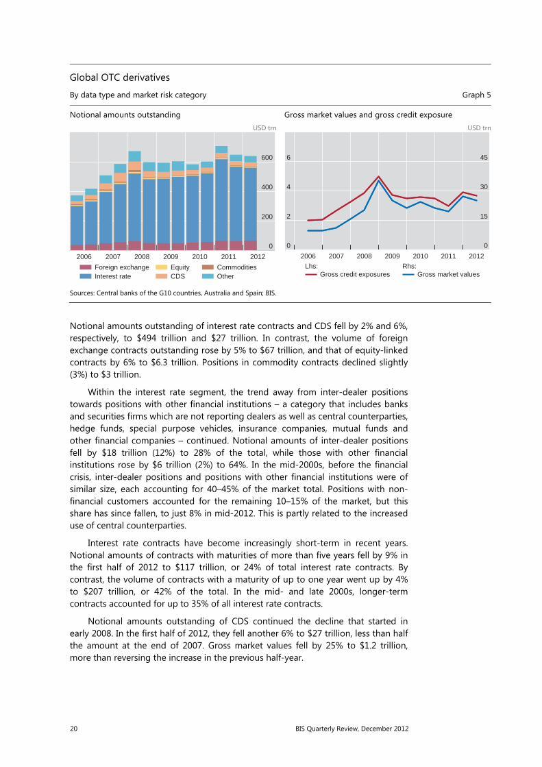
Positions in the OTC derivatives market continued to decline in the first half of 2012. Notional amounts outstanding – or the face value – of all contracts fell to $639 trillion at the end of June 2012 (Graph 5), 10% lower than the high recorded 12 months previously and 1% lower than at end-2011.7 Gross market values, which measure the cost of replacing existing contracts, dropped by 7% to $25 trillion. Gross credit exposures, which measure reporting dealers’ exposure after taking account of legally enforceable netting agreements and thus provide a measure of counterparty risk in the OTC derivatives market, declined to $3.7 trillion.

Smaller positions in the interest rate and credit default swap (CDS) segments more than offset slight increases in foreign exchange and equity-linked contracts.

7 The decline relative to June 2011 is even larger if one corrects for the expansion in the reporting

population. Australia and Spain joined the previous reporters Belgium, Canada, France, Germany, Italy, Japan, the Netherlands, Sweden, Switzerland, the United Kingdom and the United States in December 2011, adding approximately $13 trillion to notional amounts outstanding.


Notional amounts outstanding of interest rate contracts and CDS fell by 2% and 6%, respectively, to $494 trillion and $27 trillion. In contrast, the volume of foreign exchange contracts outstanding rose by 5% to $67 trillion, and that of equity-linked contracts by 6% to $6.3 trillion. Positions in commodity contracts declined slightly (3%) to $3 trillion.

Within the interest rate segment, the trend away from inter-dealer positions towards positions with other financial institutions – a category that includes banks and securities firms which are not reporting dealers as well as central counterparties, hedge funds, special purpose vehicles, insurance companies, mutual funds and other financial companies – continued. Notional amounts of inter-dealer positions fell by $18 trillion (12%) to 28% of the total, while those with other financial institutions rose by $6 trillion (2%) to 64%. In the mid-2000s, before the financial crisis, inter-dealer positions and positions with other financial institutions were of similar size, each accounting for 40–45% of the market total. Positions with non-financial customers accounted for the remaining 10–15% of the market, but this share has since fallen, to just 8% in mid-2012. This is partly related to the increased use of central counterparties.

Interest rate contracts have become increasingly short-term in recent years. Notional amounts of contracts with maturities of more than five years fell by 9% in the first half of 2012 to $117 trillion, or 24% of total interest rate contracts. By contrast, the volume of contracts with a maturity of up to one year went up by 4% to $207 trillion, or 42% of the total. In the mid- and late 2000s, longer-term contracts accounted for up to 35% of all interest rate contracts.

Notional amounts outstanding of CDS continued the decline that started in early 2008. In the first half of 2012, they fell another 6% to $27 trillion, less than half the amount at the end of 2007. Gross market values fell by 25% to $1.2 trillion, more than reversing the increase in the previous half-year.

Global OTC derivatives

By data type and market risk category Graph 5

Notional amounts outstanding USD trn

Gross market values and gross credit exposure USD trn

Sources: Central banks of the G10 countries, Australia and Spain; BIS.

0

200

400

600

2006 2007 2008 2009 2010 2011 2012

Foreign exchangeInterest rate

EquityCDS

CommoditiesOther

0

2

4

6

0

15

30

45

2006 2007 2008 2009 2010 2011 2012

Gross credit exposuresLhs:

Gross market valuesRhs:


Box 3: The importance of reference rates

Christian Upper

Libor, Euribor and similar rates have become the key reference or benchmark rates used in contracts such as interest rate derivatives, floating rate loans and mortgages, with hundreds of trillions of dollars outstanding. Libor wasintroduced in 1986 as an alternative to Treasury bill (T-bill) and bilaterally negotiated interest rates in floating rate loans and interest rate swaps. This private sector initiative filled an important gap: T-bill rates had become poor proxies for marginal funding costs for the larger globally active banks owing to the flight to quality following theLatin American debt crisis. Furthermore, bilaterally negotiated benchmarks were cumbersome to use. Thanks to the great convenience of having a single benchmark for trading interest rate risk, the use of Libor and similarbenchmarks grew rapidly. However, since 2008 the reliability and integrity of Libor and other reference rates havebeen called into question by evidence that some contributors misstated their borrowing costs.

This box provides evidence on how widely reference rates such as Libor and Euribor are used. We estimate that 14% of all outstanding bonds pay interest that is linked to an identifiable reference rate, and 79% pay a fixed rate;the rate on the remaining 7% cannot be identified with the available data (Graph B). The proportion of variable rate bonds linked to an identifiable reference rate varies across currencies, ranging from 1% for the Japanese yen to 19%for sterling. In the syndicated loan market, the proportion of debt whose interest payments are linked to identifiable reference rates is much higher. At least 54% of the loans originated between October 2011 and September 2012 arelinked to Libor, Euribor or a similar reference rate. For the remaining loans, we do not have any information on whether they are linked to a particular reference rate.

Although several benchmark rates are available for most currencies, the vast majority of bonds and syndicatedloan contracts are linked to a single benchmark. For instance, 98% of all euro-denominated floating rate bonds and 91% of the syndicated loans with identified benchmarks in that currency are linked to Euribor (Graph C). Euro Liborexists, but seems to be little used in debt markets. By contrast, the US dollar market is dominated by Libor, with 99%of floating rate bonds and syndicated loans with identifiable benchmarks linked to this particular rate. It isinteresting to go beyond the top currencies and look at smaller markets. Some, such as the Swiss franc market, aredominated by Libor, which even serves as policy rate for the Swiss National Bank. By contrast, both the Australianand Canadian dollar markets are dominated by local benchmark rates.

Benchmark rates for bonds and syndicated loans

In trillions of US dollars Graph B

Bonds1 Syndicated loans2

1 Securities outstanding at end-September 2012 for which the base rate is specified (ie linked or fixed) or unspecified (not known) by Dealogic. 2 Syndicated credit facilities signed between 1 October 2011 and 30 September 2012 for which the reference rate is specified (ie linked) or unspecified (not known) by Dealogic.

Sources: Dealogic; BIS calculations.

0.0

7.5

15.0

22.5

30.0

AUD CAD CHF EUR GBP JPY USD

Fixed Not known Linked

0.0

0.5

1.0

1.5

2.0


Not known Linked


Benchmark rates for bonds and syndicated loans

In per cent Graph C

Bonds1 Syndicated loans2

1 Securities outstanding at end-September 2012 for which the reference rate is linked to Euribor, Libor or some other rate. 2 Syndicatedcredit facilities signed between 1 October 2011 and 30 September 2012 for which the reference rate is linked to Euribor, Libor or someother rate.

Sources: Dealogic; BIS calculations.

See R McCauley, “Benchmark tipping in the money and bond markets”, BIS Quarterly Review, March 2001, pp 39–45. See UnitedKingdom Financial Services Authority, Final Notice to Barclays Bank Plc, 27 June 2012, for a particularly well documented case. Similarallegations have been made in other jurisdictions and have led to prosecution. See The Wheatley Review of Libor: final report, September2012, available at www.hm-treasury.gov.uk/wheatley_review.htm, for the UK authorities’ response.

The decline in open positions in the CDS market mainly affected contracts referencing non-financial firms. Notional amounts of such contracts fell by 10% to $10 billion. CDS referencing sovereign debt or debt issued by financial institutions remained relatively stable at $3 trillion and $7 trillion, respectively.

0

25

50

75

100


Euribor Libor Other

0

25

50

75

100


Euribor Libor Other


Sebastian von Dahlen

[email protected]

Goetz von Peter

[email protected]

Natural catastrophes and global reinsurance – exploring the linkages1

Natural disasters resulting in significant losses have become more frequent in recent decades, with 2011 being the costliest year in history. This feature explores how risk is transferred within and beyond the global insurance sector and assesses the financial linkages that arise in the process. In particular, retrocession and securitisation allow for risk-sharing with other financial institutions and the broader financial market. While the fact that most risk is retained within the global insurance market makes these linkages appear small, they warrant attention due to their potential ramifications and the dependencies they introduce.

JEL classification: G22, L22, Q54.

The physical destruction caused by severe natural catastrophes triggers a series of adverse effects. Damaged production facilities, shattered transportation infrastructure and business interruption produce both direct losses and indirect macroeconomic costs in the form of foregone output (von Peter et al (2012)). Beyond these economic costs are enormous human suffering and a host of longer-term socioeconomic consequences, documented by the World Bank and United Nations (2010).

By examining catastrophe-related losses over the past three decades, this special feature explores the linkages that arise in the transfer of risk from policyholders all the way to the ultimate bearer of risk. It describes the contracts and premiums exchanged for protection, and the way reinsurers diversify and retain risks on their balance sheets. In so doing, the feature traces how losses cascade through the system when large natural disasters occur. Losses from insured property and infrastructure first affect primary insurers, who in turn rely on reinsurers to absorb peak risks – low-probability, high-impact events. Reinsurers, in turn, use their balance sheets and, to a lesser extent, retrocession and securitisation arrangements, to manage peak risks across time and space.2

1 The views expressed in this article are those of the authors and do not necessarily reflect those of

the BIS, the IAIS or any affiliated institution. We would like to thank Anamaria Illes for excellent research assistance, and Claudio Borio, Stephen Cecchetti, Emma Claggett, Daniel Hofmann, Anastasia Kartasheva, Andrew Stolfi and Christian Upper for helpful comments.

2 Retrocession takes place when a reinsurer buys insurance protection from another entity. Securitisation refers to the transfer of insurance-related risks (liabilities) to financial markets.


This global risk transfer creates linkages within the insurance industry and between insurers and financial markets. While securitisation to financial markets remains relatively small, linkages between financial institutions produced through retrocession have not been fully assessed as detailed data are lacking. Further linkages can arise when reinsurers go beyond their traditional insurance business to engage in financial market activities such as investment banking or CDS writing; the implications of those activities are beyond the scope of this feature.3 Comprehensive information is needed to monitor the entire risk transfer cascade and assess its wider repercussions in financial markets.

Physical damage and financial losses

Natural catastrophes resulting in significant financial losses have become more frequent over the past three decades (Kunreuther and Michel-Kerjan (2009), Cummins and Mahul (2009)). The year 2011 witnessed the greatest natural catastrophe-related losses in history, reaching $386 billion (Graph 1, top panel). The trend in loss developments can be attributed in large measure to weather-related events (Graph 1, bottom right-hand panel). And losses have been compounded by rising wealth and increased population concentration in exposed areas such as coastal regions and earthquake-prone cities.

These factors translate into greater insured losses where insurance penetration is high. At $110 billion, insured losses in 2011 came close to the 2005 record of $116 billion (in constant 2011 dollars). The reinsurance sector absorbed more than half of insured catastrophe losses in 2011. This considerable burden on reinsurers reflected the materialisation of various peak risks, notably in Japan, New Zealand, Thailand and the United States.

The level of insured losses also depends on catastrophes’ geography and physical type. The bottom panels of Graph 1 show that losses due to earthquakes (geophysical events) have been less insured on average than those from storms (meteorological events). The highest economic losses caused by geophysical events occurred in 2011 in the wake of the Great East Japan earthquake and tsunami ($210 billion), for which private insurance coverage was relatively low at 17% (left-hand panel).4 Droughts can be even more difficult to quantify and insure. By contrast, the right-hand panel of Graph 1 shows that meteorological events produced record losses in 2005, when Hurricanes Katrina, Rita and Wilma devastated a region of the US Gulf Coast having 50% or more in insurance coverage.

The volume of insured losses differs substantially across continents, depending on the availability of and demand for insurance. While overall a slight upward trend can be discerned over the past 10 years, the wide dispersion in insurance density indicates that the stage of a region’s economic development plays an important role (Graph 2, left-hand panel). Residents of North America, Oceania and Europe spend significant amounts on non-life (property and casualty) insurance, whereas

3 The interested reader is referred to IAIS (2012). 4 Mandatory insurance, however, can push the effective insurance coverage to near 80%, as in Chile’s

and New Zealand’s earthquakes of 2010 and 2011.


many populous countries in Latin America, Asia and Africa host underdeveloped insurance markets. Poor countries typically lack the financial and technical capacity to provide affordable insurance coverage. For example, less than 1% of the staggering economic losses due to Haiti’s 2010 earthquake were insured. The pattern of insured losses thus only partly reflects the geography of natural catastrophes.

North America accounts for the largest insured losses associated with natural disasters (Graph 2, right-hand panel). In 23 of the 32 years since 1980, more than half of global insured losses originated in the region, though part of this volume was redistributed through global reinsurance companies. Asia, Oceania and, to a lesser extent, Latin America saw increases in catastrophe-related losses on the back

Natural catastrophes: frequencies and losses1 Graph 1

All natural catastrophes Frequency USD bn

Earthquakes and other geophysical events2 Frequency USD bn

Storms and other meteorological events3 Frequency USD bn

1 Includes all natural catastrophes reported to have caused property damage since 1980. “Major catastrophes” are events causing morethan 100 fatalities or more than $250 million in losses. Losses are expressed in terms of constant 2011 US dollars using the US CPI, and derive primarily from damage to property and infrastructure. 2 Earthquakes, volcanic eruptions and dry mass movement (landslides) and their direct consequences (eg the tsunami following Japan’s earthquake in 2011). 3 Storms and their direct consequences (eg the flooding following Hurricanes Katrina, Rita and Wilma in 2005).

Sources: Centre for Research on the Epidemiology of Disasters EM-DAT database; MunichRe NatCatSERVICE; authors’ calculations.

0

250

500

750

1,000

0

100

200

300

400

1980 1985 1990 1995 2000 2005 2010

All catastrophesMajor catastrophes

Lhs:Insured lossesUninsured losses

Rhs:

0

20

40

60

80

100

0

50

100

150

200

250

80 85 90 95 00 05 10

All geophysical catastrophesMajor geophysical catastrophes


Rhs:

0

100

200

300

400

500

0

50

100

150

200

250

80 85 90 95 00 05 10

All meteorological catastrophesMajor meteorological catastrophes


Rhs:


of rising insurance density over the past 10 years. Correspondingly, these three regions account for a rising share of insured losses.

Insurance density and catastrophe losses Graph 2

Insurance density by continent1 USD/capita

Insured losses associated with natural catastrophes USD bn

1 Insurance density is measured as the premium per capita that insurance companies receive for domestically insuring non-life (property and casualty) risks. 2 Australia, New Zealand and Pacific islands.

Sources: MunichRe NatCatSERVICE; SwissRe Sigma database; authors’ calculations.

Risk transfer

Natural catastrophe-related losses are large and unpredictable. The insured losses shown in Graphs 1 and 2 reflect recent experience. This section describes the sequence of payments based on contractual obligations that is triggered when an insured event materialises.

One can think of the insurance market as organising risk transfer in a hierarchical way. Losses cascade down from insured policyholders to the ultimate bearers of risk (Graph 3). When catastrophe strikes, the extent of physical damage determines total economic losses, a large share of which is typically uninsured. The insured losses, however, must be shouldered by the global insurance market (Graph 3, light grey area). The public sector, when it insures infrastructure, often does so directly with reinsurers through public-private partnerships, although more data would be necessary to pin down the exact scope worldwide.5 The majority of the losses relate to private entities contracting with primary insurers, the firms that locally insure policyholders against risks.

Claims for reimbursement thus first affect primary insurers. But they absorb only some of the losses, having ceded (transferred) a share of their exposure to reinsurance companies. Reinsurers usually bear 55–65% of insured losses when a

5 For example, in the late 1990s the Mexican government established a mechanism to support the

rapid rehabilitation of federal and state infrastructure affected by natural disasters (Fonden), in which reinsurers play a key role in transferring risks outside Mexico.

0

500

1,000

1,500

2,000

02 03 04 05 06 07 08 09 10

North AmericaAsiaEuropeOceania2

Latin America and CaribbeanAfricaWorld (average)

0

25

50

75

100

00 01 02 03 04 05 06 07 08 09 10 11

North AmericaAsiaEuropeOceania2

Latin America and CaribbeanAfrica


large natural disaster occurs. They diversify concentrated risks among themselves and pass a fraction of losses on to the broader financial market, while ultimately retaining most catastrophe-related risk (see section below).

Before disaster strikes, however, there is a corresponding premium flow in exchange for protection. Based on worldwide aggregate premium payments in 2011, policyholders and insured entities, both private and public sector, spent $4,596 billion to receive insurance protection. Some 43% of this global premium volume ($1,969 billion) relates to non-life insurance and the remainder to life insurance products (IAIS (2012)). Primary insurers, in turn, paid close to $215 billion to buy coverage from reinsurers. The lion’s share, nearly $165 billion, came from primary insurers active in the non-life business. About one third of this amount, $65 billion, was geared towards protection against peak risks, with $18 billion for specific natural catastrophe contracts. By way of comparison, life insurance

Catastrophe risk transfer in 2011 Graph 3

The size of the arrows is proportional to the volume of losses caused by natural catastrophes in 2011. Reinsured losses are estimated from the average reinsurance share of insured peak losses for major natural catastrophes (0.6 * $106 billion = $64 billion). In line with this estimate, seven of the 10 largest reinsurance companies, accounting for about 40% of the market, declared a combined $26.4 billion in catastrophe-related losses in their 2011 annual reports. Losses transferred via retrocession are estimated by apportioning insured losses in proportion to the premium payments the ultimate bearers received in 2011. The loss-sharing with financial markets comes from a triggered catastrophe bond.

Sources: Company reports; authors’ calculations and estimates.

Losses fromphysical damage

$386bn

Primary insurers

Reinsurers

Retrocession$7.9bn

Natural catastrophes

Insured entities

Private Public

Globalinsurancemarket

Insuredlosses

$110bn

Reinsuredlosses$64bn

Other financial institutionsFinancial markets

Retrocession $1.6bnSecuritisation $0.3bn


companies spent 2% of their premium income, $40 billion, on reinsurance protection. This comparatively low degree of reinsurance protection is due to the fact that results are typically less volatile in life insurance than in non-life insurance. Following any risk transfer, insurers remain fully liable vis-à-vis the policyholder based on the initial contractual obligations, regardless of whether or not the next instance pays up on the ceded risk.

Reinsurance companies, in turn, buy protection against peak risks from other reinsurers and financial institutions. In this process of retrocession, reinsurers spent $25 billion in 2011 to mitigate their own downside risk. The bulk of this amount represents retroceded risks transferred to other reinsurance companies ($20 billion in premiums), while a relatively small share is ceded to other market participants such as hedge funds and banks ($4 billion) and financial markets ($1 billion).

An important aspect of this structure is the prefunding of insured risks. Premiums are paid ex ante for protection against an event that may or may not materialise over the course of the contract. These payments by policyholders and insurers generate a steady premium flow to insurers and reinsurers, respectively. Only if and when an event with the specified characteristics occurs are the claims payments shown in Graph 3 triggered. At all other times, premium flows are accumulated in the form of assets held against technical reserves (see next section).

Reinsurance contracts come in two basic forms which differ in the way primary insurers and reinsurers determine premiums and losses. Proportional reinsurance contracts share premiums and losses in a predefined ratio. Since the 1970s, non-proportional contracts have increasingly been used as a substitute. Instead of sharing losses and premiums in fixed proportions, both parties agree on the insured risks and calculate a specific premium on that basis. The typical non-proportional contract specifies the amount beyond which the reinsurer assumes losses, up to an agreed upon ceiling (first limit). Depending on the underlying exposure, a primary insurer may decide to buy additional layers of reinsurance cover, for example with other reinsurers, on top of the first limit.

“Excess of loss” agreements are the most common form of non-proportional reinsurance cover. For natural catastrophes, these contracts are known as CatXL (catastrophe excess of loss) and cover the loss exceeding the primary insurer’s retention for a single event. A major earthquake, for example, is likely to affect the entire portfolio of a primary insurer, leading to thousands of claims in different lines of business, such as motor, business interruption and private property insurance. As a result, primary insurers often purchase CatXL coverage to protect themselves against peak risks.

Peak risks and the reinsurance market

A reinsurer’s balance sheet reflects its current and past acceptance of risks through its underwriting activity. Dealing with exposure to peak risks, which relate to natural catastrophes, is the core business of the reinsurance industry. Natural catastrophes are rooted in idiosyncratic physical events such as earthquakes. When underwriting natural catastrophe risks, reinsurers can rely to a large extent on the fact that physical events do not correlate endogenously in the way financial risk does. To


achieve geographical diversification, reinsurers offer peak risk protection not just for one country but ideally on a worldwide basis.6

Another form of diversification takes place over time. Premiums are accumulated over years, and claims payments are usually paid out over the course of months or sometimes years. Graph 4 (left-hand panel) shows the average payout profile for CatXL contracts. Statistics on reinsurance payments show that claims are typically settled over an extended period. On average, 63% of the ultimate obligations are paid within a year and 82% within two years, and it takes more than five years after a natural disaster strikes for the cumulative payout to reach 100%.

The premium inflows not immediately used for paying out claims are invested in various assets held for meeting expected future claims. In this way, reinsurers build specific reserves called technical provisions.7 These constitute the largest block of reinsurers’ on-balance sheet liabilities (Graph 4, right-hand panel). Insured losses are met by running down assets in line with these technical reserves. Losses in any one year typically lead to loss ratios (incurred losses as a share of earned premium) of between 70 and 90%. To determine whether a reinsurer can withstand severe and unprecedented (yet plausible) reinsured events, regulators look for sufficient technical provisions and capital on the reinsurer’s balance sheet.

The occurrence of a major natural catastrophe dents reinsurers’ underwriting profitability, as reflected in the combined ratio. This indicator sets costs against premium income.8 A combined ratio above 100% is not sustainable for an extended

6 For instance, the exposure to certain types of natural catastrophes is higher in the United States

than in Europe. To diversify, US insurers cede (transfer) nearly twice as much in premium volume to European reinsurers than European insurers cede to US reinsurers.

7 In addition, the catastrophe reserve is accumulated as a buffer for large unexpected losses. 8 The combined ratio is computed as 100 * (losses + expenses) / (premium income).

Catastrophe payouts and reinsurers’ balance sheets Graph 4

Reinsurance payout profile1 Per cent

Generic balance sheet of reinsurance companies2 Per cent

1 Cumulative percentage of ultimate payout on catastrophe excess of loss contracts, based on worldwide observations with respect to thehistorical paid loss development until 2011. 2 Combined balance sheet of the five largest reinsurance companies outside Gen Re andLloyd’s, normalised to express percentage breakdown.

Sources: Reinsurance Association of America; ISIS database on insurance companies worldwide; company information; authors’ calculations.

0

20

40

60

80

100

0 2 4 6 8 10 12 14 16 18 20Quarters after natural castastrophe

0

20

40

60

80

100

Assets Liabilities

81% Investments

7% Retrocession recoverable

12% Other

71% Technical provisions

11% Shareholder equity

18% Other


period.9 By contrast, temporary spikes in the combined ratio are indicative of one-off extreme events which can be absorbed by an intertemporal transfer of risk. The combined ratio spiked in the years featuring the most costly natural catastrophes to date (Graph 5, blue line): 2005, the year of major hurricanes in the US, and 2011, following earthquakes and flooding in Asia and Oceania. Both occasions also reduced the stock of assets reserved for meeting claims. Yet these temporary spikes in the combined ratio did not cut through to shareholder equity to any significant extent. Catastrophes affect equity only if losses exceed the catastrophe reserve.

Recent market developments caused shareholder equity to decrease more than insurers’ core underwriting business ever has. During the global financial crisis of 2008–09, shareholder equity (book value) declined by 15% (Graph 5, red line), and insurance companies’ share prices dropped by 59% (yellow line), more than after any natural catastrophe to date. In contrast, shareholder equity remained resilient in 2005 and 2011, when reinsurers weathered record high catastrophe losses.

In dealing with the consequences of peak catastrophe risks, the industry has gravitated towards a distinctive market structure. One important element is the size of reinsurance companies. Assessing and pricing a large number of different potential physical events involves risk management capabilities and transaction costs on a large scale. Balance sheet size is therefore an important tool for a reinsurer to attain meaningful physical diversification on a global scale. Partly as a result, the 10 largest reinsurance companies account for more than 40% of the global non-life reinsurance market (Graph 6, right-hand panel).

9 That said, when financial market conditions were favourable, some insurance companies pursued a

business model of loose underwriting standards and low risk premiums, believing that their investment returns would compensate for their elevated combined ratio. These companies were particularly exposed when markets deteriorated.

Reinsurance financial indicators1 Graph 5

End-Dec 2007 = 100

1 The vertical lines indicate the dates of Hurricanes Katrina (29 August 2005), Rita (24 September 2005) and Wilma (22 October 2005) and the Great East Japan earthquake and tsunami (11 March 2011). The shaded area represents the period between the Lehman Brothers bankruptcy (15 September 2008) and the equity market trough (9 March 2009). 2 The MSCI insurance sub-index and shareholder equityare rebased: 31 December 2007 = 100. The combined ratio weighted is in per cent. 3 Ten largest companies, excluding Berkshire Hathaway and Reinsurance Group of America, weighted by their yearly respective market share in gross premium income. The combined ratio expresses losses plus expenses as a share of premium income.

Sources: Bloomberg; Standard & Poor’s, Global Reinsurance Highlights; authors’ calculations.

25

40

55

70

85

100

65

75

85

95

105

115

2004 2005 2006 2007 2008 2009 2010 2011

MSCI World insurance sub-index2Lhs:

Weighted shareholder equity2, 3

Weighted combined ratio3

Rhs:


In spite of the reinsurance market’s size and concentration, failures of reinsurance companies have remained limited in scope. The largest failures to date, comprising two bankruptcies in 2003, led to an essentially inconsequential reduction in available reinsurance capacity of 0.4% (Graph 6, left-hand panel). That said, any failure of a reinsurer leads to a loss of reinsurance recoverables by primary insurers, and could cause broader market tensions in the event of a disorderly liquidation of large portfolios.

In this respect, the degree of connectedness within the global insurance market plays an important role. Based on their business model, reinsurers enter into contracts with a large number of primary insurance companies, giving rise to numerous vertical links (Graph 3). In addition, risk transfer between reinsurers leads to horizontal linkages.10 We estimate that 12% of natural catastrophe-related risk accepted by reinsurers is transferred within the reinsurance industry, which implies that the industry as a whole retains most of the risks it contracts. In 2011, reinsurers paid 3% of earned premiums to cede catastrophe risk to entities outside the insurance sector. Judging by premium volume, the global insurance market transfers a similarly small share of accepted risk to other financial institutions and the wider financial markets.

Linkages with financial markets

Arrangements designed to transfer risk out of the insurance sector create linkages with other financial market participants. Retrocession to other financial institutions uses contractual arrangements similar to those between reinsurers, and commits 10 For example, a reinsurer might exchange some of its exposure to earthquake risk in Japan for US

flood risk with another reinsurer.

Reinsurance market developments Graph 6

Reinsurance market concentration Per cent

Failures of reinsurance companies Per cent of premiums Number of companies

1 Market share of the 10 largest reinsurance companies, measured as a share of gross premiums written by reinsurance companiesworldwide in the non-life (property and casualty) business. 2 In relation to total market size as measured by gross premiums written (premiums ceded by insurers to reinsurance companies). 3 Number of failures of reinsurance companies worldwide, per calendar year.

Sources: IAIS, based on industry data; authors’ calculations.

30

40

50

60

00 01 02 03 04 05 06 07 08 09 10 11

Top 10 market share1

0.0

0.1

0.2

0.3

0.4

0

1

2

3

4

80 83 86 89 92 95 98 01 04 07 10

Market share of failed companies2Lhs:

Number of failures3Rhs:


banks and other financial institutions to pay out if the retroceded risk materialises. Securitisation, on the other hand, involves the issuance of insurance liabilities to the wider financial market.11 The counterparties are typically other financial institutions, such as hedge funds, banks, pension funds and mutual funds.

Among insurance-linked securities, catastrophe bonds are the main instrument for transferring reinsured disaster risks to financial markets. The exogenous nature of the underlying risks supports the view that catastrophe bonds provide effective diversification unrelated to financial market risk. For these reasons, industry experts had high expectations for the expansion of the catastrophe bond market (eg Jaffee and Russell (1997), Froot (2001)).

The issuance of catastrophe bonds involves financial transactions with a number of parties (Graph 7). At the centre is a special purpose vehicle (SPV) which funds itself by issuing notes to financial market participants. The SPV invests the proceeds in securities, mostly government bonds which are held in a collateral trust. The sponsoring reinsurer receives these assets in case a natural disaster materialises as specified in the contract. Verifiable physical events, such as storm intensity measured on the Beaufort scale, serve as parametric triggers for catastrophe bonds.12 Investors recoup the full principal only if no catastrophe occurs. In contrast

11 This form of securitisation differs from the practice in credit markets in two ways: the securitised

item is an insurance liability, and the sponsoring insurer retains ultimate liability should the counterparty fail to pay.

12 Such parametric solutions prevail because they are triggered by a predefined physical event and hence provide immediate clarity for all parties involved. Less common are, for example, indemnity solutions, where the trigger is based on actual losses, because it often takes a significant amount of time to determine the full loss amount.

Securitisation of natural catastrophe risk Graph 7

The solid black lines show payments made ex ante with certainty. The green arrow depicts repayment that takes place if the specified catastrophe does not materialise. If the catastrophe occurs, the investments are liquidated and proceeds are transferred to the sponsoring reinsurance company for meeting claims.

1 Special purpose vehicle that issues natural catastrophe bonds and places assets in a trust fund.

Sources: National Association of Insurance Commissions and Center for Insurance Policy and Research; authors’ adaptation.

Reinsurancecompany

Financialmarket

investors

Swap counterparty

SPV 1

Scheduledinterest

Investmentearnings

Transfer

Premiumpayments

Investments

A L

Catastrophebonds

Repayment ofprincipal

Interestpayments

Cash for bonds

If no catastropheIf catastrophe


to other bonds, the possibility of total loss is part of the arrangement from inception, and is compensated ex ante by a higher coupon.

Despite experts’ high expectations, the catastrophe bond market has remained relatively small. Bond issuance has never exceeded $7 billion per year, limiting the outstanding capital at risk to $14 billion (Graph 8). Very few catastrophe bonds have been triggered to date. The 2005 Gulf Coast hurricanes activated payouts from only one of nine catastrophe bonds outstanding at the time (IAIS (2009)). Likewise, the 2011 Japan earthquake and tsunami triggered one known catastrophe bond, resulting in a payout of less than $300 million. Payouts to reinsurers from these bonds are small when compared to the sum of insured losses ($116 billion in 2005 and $110 billion in 2011).

The global financial crisis has also dealt a blow to this market. The year 2008 saw a rapid decline in catastrophe bond issuance, reflecting generalised funding pressure and investor concern over the vulnerability of insurance entities. The crisis also demonstrated that securitisation structures introduce additional risk through linkages between financial entities. A case in point was the Lehman Brothers bankruptcy in September 2008. Four catastrophe bonds were impaired – not due to natural catastrophes, but because they included a total return swap with Lehman Brothers acting as a counterparty. Following Lehman’s failure, these securitisation arrangements were no longer fully funded, and their market value plunged. Investors thus learned that catastrophe bonds are not immune to “unnatural” disasters such as major institutional failures.13

A further set of financial linkages arises with other financial institutions through cross-holdings of debt and equity. Insurance companies hold large positions in fixed income instruments, including bank bonds. At the same time, other financial entities own bonds and stocks in insurance companies. For instance, the two largest reinsurance companies stated in their latest (2011) annual reports that Warren

13 Following this episode, sponsors of catastrophe bonds employed other types of collateral

arrangements in lieu of total return swaps. There has recently been a shift towards the use of government bonds as collateral.

Catastrophe bond issuance by type of risk1 Graph 8

USD bn

1 Data before 2003 are not broken down by type. 2 Includes mortality, peril, life and worldwide risks. 3 Values are year-to-date, thus the value for 2012 is not final.

Sources: Artemis; Guy Carpenter.

0

3

6

9

12

96 97 98 99 00 01 02 03 04 05 06 07 08 09 10 11 12

EarthquakeWeather

Weather/earthquakeWeather/mortality

Life and other2 Risk capital outstanding at year-end3


Buffett and his companies (Berkshire Hathaway Inc, OBH LLC, National Indemnity Company) own voting rights in excess of the disclosure threshold (10% in one case and 3.10% in another). Additional shareholders with direct linkages to the financial sector have been disclosed by a number of reinsurance companies. The ramifications of such linkages in this part of the market are difficult to assess.

Conclusion

The upward trend in overall economic losses in recent decades highlights the global economy’s increasing exposure to natural catastrophes. This development has led to unprecedented losses for the global insurance market, where they cascade from the policyholders via primary insurers to reinsurance companies. Reinsurers cope with these peak risks through diversification, prefunding and risk-sharing with other financial institutions.

This global risk transfer creates linkages within the insurance industry and between insurers and financial markets. While securitisation to financial markets remains relatively small, linkages between financial institutions arising from retrocession have not been fully assessed. It is important for regulators to have access to the data needed for monitoring the relevant linkages in the entire risk transfer cascade, as no comprehensive international statistics exist in this area.


References

Cummins, D and O Mahul (2009): “Catastrophe risk financing in developing countries – principles for public intervention”, World Bank.

Froot, K (2001): “The intermediation of financial risk: evolution of the catastrophe reinsurance market”, Journal of Financial Economics, no 60, pp 529–71.

IAIS (2009): “Developments in (re)insurance securitisation”, Global Reinsurance Market Report, mid-year edition, Basel, August.

——— (2012): “Reinsurance and financial stability”, Policy Paper, Basel, July.

Jaffee, D and T Russell (1997): “Catastrophe insurance, capital markets, and uninsurable risk”, Journal of Risk and Insurance, vol 64, no 2, pp 205–30.

Kunreuther, H and E Michel-Kerjan (2009): “At war with the weather: managing large-scale risks in a new era of catastrophes”, MIT Press.

von Peter, G, S von Dahlen and S Saxena (2012): “Unmitigated disasters? New evidence on the macroeconomic cost of natural catastrophes“, BIS Working Papers, no 394.

World Bank and United Nations (2010): “Natural hazards, unnatural disasters – the economics of effective prevention”, World Bank.


Stefan Avdjiev

[email protected]

Zsolt Kuti

[email protected]

Előd Takáts

[email protected]

The euro area crisis and cross-border bank lending to emerging markets1

Cross-border bank lending to emerging markets dropped sharply in the second half of 2011 as the euro area crisis intensified. We use the BIS international banking statistics to identify the key drivers of this decline. Our results indicate that the latest contraction in cross-border bank lending was largely linked to the deteriorating health of euro area banks.

JEL classification: F34, G15, G21.

As the euro area crisis intensified in the second half of 2011, cross-border bank lending to emerging market economies (EMEs) dropped sharply (Graph 1). The decline marked the end of the continuous nine-quarter recovery that followed the post-Lehman contraction in 2008–09. Furthermore, the recovery in the first quarter of 2012 came to an abrupt halt in the second. This raises questions for policymakers: what caused this lending decline? Was it that demand for credit fell in EMEs? Did country risk rise? Or were the key drivers linked to the health of the advanced economy banks that supply EMEs with cross-border credit? And, if yes, which banking systems contributed the most to the decline?

We answer these questions by using the BIS international banking statistics (IBS) in a panel regression framework. The analysis covers quarterly cross-border bank lending data for 40 EMEs between the third quarter of 2005 and the second quarter of 2012. We develop a new methodology which combines information from the two main BIS IBS data sets. This novel approach is the first to simultaneously use actual exchange rate-adjusted cross-border lending flows to EMEs and trace these flows to individual home country banking systems.

We use the panel regression results to decompose the quarterly fluctuations in cross-border lending to EMEs into components attributable to EME credit demand, EME country risk and the health of the banking systems that supply the cross-border credit.

Our results indicate that home country factors related to the health of advanced economy banks played a crucial role during the late 2011 lending 1 The authors thank Claudio Borio, Stephen Cecchetti, Dietrich Domanski, Patrick McGuire, Nikola

Tarashev, Christian Upper and Adrian van Rixtel for useful comments and discussions. Bat-el Berger provided excellent research assistance. The views expressed are those of the authors and do not necessarily reflect those of the BIS.


downturn. Furthermore, by allocating the contributions of home country factors to national banking systems, we find that euro area banks accounted for most of the explained contraction in cross-border credit during the second half of 2011. The negative impact of euro area banks was especially pronounced in emerging Europe.

This special feature is organised as follows. The first section introduces the data. The second details the regression analysis used to identify home and host country factors, and the third decomposes cross-border lending flows according to these factors. The fourth discusses the methodology and the main results. The final section concludes with some policy implications.

Data

We use both main data sets from the BIS international banking statistics. The first data set, the BIS locational banking statistics by residence (“locational data set” hereafter), defines creditors and debtors according to their residence, consistently with national accounts and balance of payments principles. The second data set, the BIS consolidated banking statistics (“consolidated data set” hereafter), groups cross-border claims according to the nationality of banks (ie according to the location of banks’ headquarters), netting out inter-office positions. For instance, if an Italian bank’s Austrian subsidiary lends to a firm in Hungary, then the locational data set would register the loan as an Austrian claim on Hungary; by contrast, the consolidated data set would record it as an Italian bank’s claim on Hungary.

Each of the two data sets has distinct advantages. On the one hand, in the locational data set, the quarterly changes in banks’ cross-border claims are adjusted for exchange rate fluctuations. This is not the case in the consolidated data set, where the currency composition of cross-border claims is unknown. From this perspective, therefore, the locational data set is a better choice, since periods of large contractions in cross-border lending to EMEs tend to coincide with significant exchange rate movements.

Adjusted flows to emerging economies Graph 1

USD bn


–300

–200

–100

0

100

200

2005 2006 2007 2008 2009 2010 2011 2012

Emerging EuropeEmerging Latin America and Caribbean

Emerging Africa and Middle EastEmerging Asia and Pacific

Emerging economies total


On the other hand, the locational data set does not provide information on the nationality of lending banks. As a result, it cannot be used to identify the impact of potential home country constraints associated with individual banking systems. From this perspective, therefore, the consolidated data set is superior, as it can help to estimate banking system-specific home country factors.

Existing studies on the determinants of foreign bank lending to EMEs reflect these relative advantages. For instance, McGuire and Tarashev (2008) use the consolidated data set to construct the dependent variable in their model. As a consequence, they are able to study how the health of individual national banking systems affects foreign lending to EMEs, but at the expense of working with data that have not been adjusted for exchange rate fluctuations. By contrast, Takáts (2010) uses the locational data set in order to construct his dependent variable. As a result, he is able to work with exchange rate-adjusted cross-border lending flows, but cannot decompose the estimated global home country factor into banking system-specific factors.

Our approach is novel because it combines information from the locational and the consolidated data sets in a way that allows us to identify banking system-specific home country factors, while still working with exchange rate-adjusted flows. We acquire exchange rate-adjusted flows from the locational data set and employ the consolidated data set to assign weights to individual national banking systems in the construction of two financial sector stress indices, which allow us to link changes in currency-adjusted flows to individual national banking systems. While several previous studies have also used information from both of the above data sets to analyse cross-border bank lending to EMEs (McGuire and Tarashev (2008), McCauley et al (2010), Cetorelli and Goldberg (2011) and Avdjiev et al (2012)), ours is the first to relate exchange rate-adjusted cross-border bank lending flows to national banking systems.

Regression analysis

We estimate the impact of credit demand, host country risk and home country bank health on cross-border bank lending to 40 EMEs2 in a panel regression. We focus on the period between the third quarter of 2005 and the second quarter of 2012. Our dependent variable is the quarter-on-quarter growth rate in BIS reporting banks’ exchange rate-adjusted cross-border claims, obtained from the locational data set.

We construct three groups of explanatory variables. First, we use real GDP growth in the recipient country in order to identify credit demand. Second, we use EME sovereign credit default swap (CDS) spreads in order to assess the impact of perceived country risk. Finally, in order to identify home country factors, we construct two indices which measure the health of the banking systems which lend to a given EME. In both indices, we assign weights to banking systems based on

2 Argentina, Brazil, Bulgaria, Chile, China, Chinese Taipei, Colombia, Costa Rica, Croatia, the Czech

Republic, Ecuador, Egypt, Estonia, Hong Kong SAR, Hungary, India, Indonesia, Israel, Jordan, Korea, Latvia, Lithuania, Macedonia (FYR), Malaysia, Mexico, Morocco, Peru, the Philippines, Poland, Romania, Russia, Singapore, South Africa, Thailand, Tunisia, Turkey, Ukraine, Uruguay, Venezuela and Vietnam.


their share of foreign claims on that EME. We obtain these foreign claims from the consolidated data set on an immediate borrower basis.

The first index (FIcds) represents a weighted average of lending banking systems’ CDS spreads. Formally, for borrower country i at time t, the index is defined as:

(1)

where FCi,,j,t-1 stands for the outstanding stock of foreign claims of banks headquartered in country j on the residents of country i at the end of period t-1 (obtained from the consolidated data set), and CDSj,t stands for the average bank CDS spread in country j during period t.

The second index (FIvol) represents a weighted average of home country financial sector equity price volatilities. Formally, for borrower country i at time t, it is given by:

(2)

where FCi,j,t-1 is defined as above, and VOLj,t stands for the volatility of the financial sector equity sub-index in country j during period t.

The index weight assigned to each banking system is equal to its share in foreign lending to the respective EME. As a result, the indices are most sensitive to changes in the stress indicators for the banking systems that account for the largest share of foreign credit. For example, the values of the two indices for Mexico are most sensitive to changes in the stress indicators for Spanish banks, which account for the largest share of foreign lending to Mexican residents. Those same indices are much less sensitive to fluctuations in the stress levels of, say, Austrian banks, which account for a relatively minor fraction of the foreign credit in Mexico. The opposite is true for the relative weights assigned to those two banking systems in the indices for Hungary, where Austrian banks provide much more foreign credit than Spanish banks.

Equation (3) formalises the regression setup:

(3)

where XBCi,t is the outstanding stock of exchange rate-adjusted cross-border claims on country i at the end of period t (obtained from the locational data set), GDPi,t is the four-quarter moving average of real GDP of country i at period t, CDSi,t is the average sovereign CDS spread of country i during period t, FIcds

it and FIvolit are the

values of the financial sector stress indices for country i during period t, defined in equations (1) and (2), vi are country-specific fixed effects, and it is the error term.

The coefficient estimates from the regression are summarised in Table 1. The regression model is able to explain a substantial part of the total variation in the quarterly growth rate of cross-border bank lending to EMEs. All coefficients have the expected sign. Stronger GDP growth in a given EME implies higher cross-border

, , , , , ,log log cds voli t i t i t i t i t i i td XBC d GDP CDS FI FI

, , 1, ,

, , 1

i j tcdsi t j t

j i j tj

FCFI CDS

FC

, , 1, ,

, , 1

VOLi j tvoli t j t

j i j tj

FCFI

FC


bank lending to its residents, while higher EME sovereign CDS spreads imply lower lending. Increased home country banking systems’ stress levels, in terms of both CDS spreads and equity volatility, reduce cross-border bank lending.

All coefficients are statistically and economically significant. GDP growth and the two financial stress indices (FIcds and FIvol) are significant at the 1% level and the EME sovereign CDS spread at the 2% level. The estimated impact of individual independent variables is also substantial. For instance, a one percentage point increase in the real GDP growth rate in the host EME is associated with a 1.6 percentage point higher growth rate of cross-border lending to that country. A 100 basis point increase in the host EME sovereign CDS spread implies a 25 basis point decline in the growth rate of cross-border claims on that EME. Furthermore, a 100 basis point increase in the weighted average CDS spread of foreign creditor banks lowers the growth rate of cross-border credit to an EME by approximately 1.6 percentage points. Similarly, a one percentage point increase in the weighted average volatility of the financial sector equity sub-indices in the home economies reduces the growth rate of cross-border credit by roughly 30 basis points.

Decomposition analysis

We use the estimates from our regression model to decompose the fluctuations of cross-border claims on EMEs into contributions from credit demand factors, country risk factors and banking system-specific home country factors.3 We sum the contributions of FIcds and FIvol, the two banking system-specific stress indices, in order to calculate their joint impact. We allocate this joint home country factor to three nationality-based groups of banks – euro area banks, US banks and other banks.

3 In our decomposition analysis, we focus on deviations from trend. More precisely, we remove host

country-specific trends in our dependent variable by subtracting from it the constant and the country-specific fixed effects. In order to obtain the contributions of the independent variables we multiply their de-meaned realisations by the respective estimated coefficients. Importantly, this transformation is used only to ease graphical exposition and has no impact on the results: by design, all coefficients, standard errors, t-statistics and p-values in Table 1 remain unchanged in the de-meaned regression.

Regression results1

Sample period: Q3 2005 – Q2 2012 Table 1

Variables Coefficient Standard error T-statistic Probability

GDP growth (host) 1.6560 0.2587 6.40 0.0000

CDS (host) –0.0025 0.0010 –2.54 0.0112

FI CDS (home) –0.0151 0.0026 –5.69 0.0000

FI volatility (home) –0.2873 0.1010 –2.84 0.0045

R squared 0.18

Number of observations 1020 1 Regression results based on equation (3) in the main text.

Sources: BIS consolidated and locational banking statistics; Datastream; Markit; national data.


Graph 2 displays the decomposition of the de-meaned cross-border bank lending flows to EMEs. The orange line shows the average deviation of cross-border lending flows from their trend growth. The bars show the contributions of the various factors based on our estimates. Factors linked to home countries are shown in earth colours, while factors linked to host countries are represented by water colours. The gap between the bars and the line corresponds to the part of lending variation that our model does not explain, ie the role of the error term in the regression.

In line with the findings of McGuire and Tarashev (2008) and Takáts (2010), our estimates suggest that home country factors (red, brown and yellow bars combined) played a major role in driving cross-border bank lending to EMEs throughout the sample period. On average, they account for roughly half of the explained variation. The contributions of host country credit demand (light blue bars) and country risk (dark blue bars) were also significant, jointly accounting for the other half of the explained variation.

According to our estimates, the importance of home country factors increased sharply during the downturn in cross-border bank lending that took place in the second half of 2011. During this period, home country factors contributed to more than 90% of the explained contraction. By contrast, these factors accounted for only around one half of the explained contraction during the post-Lehman period.

Decomposing the estimated home country factors into impacts of national banking systems suggests that euro area banks (red bars) played a dominant role in the late 2011 contraction in cross-border bank lending to EMEs. Euro area banks were responsible for roughly 70% of the shrinkage attributed to home country factors. By contrast, the corresponding share during the post-Lehman period was approximately 40%. The results suggest that banking sector stress in the late 2011 downturn was disproportionately more concentrated on euro area banks than on their counterparts from the rest of the world. This finding confirms policy concerns, discussed for instance in BIS (2012a) and BIS (2012b), that deleveraging by euro area banks could substantially lower lending to EMEs.

Decomposition of cross-border bank flows to emerging markets

Based on the regression results in Table 1; average demeaned quarter-on-quarter changes Graph 2

Per cent

Sources: BIS consolidated and locational banking statistics; Datastream; Markit; national data; authors’ calculations.

–15

–10

–5

0

5

2006 2007 2008 2009 2010 2011 2012

Euro area banksUS banksOther banks

Home country factors:Country riskDemand

Host country factors: Cross-border flows


Reflecting the heterogeneity of EMEs, there are significant differences among the patterns observed in the four major EME regions (Graph 3). In emerging Europe, the post-Lehman decline in cross-border bank lending was somewhat milder than average (upper left-hand panel). This could reflect European banks’ commitment to the region and possibly the success of the Vienna initiative.4 However, cross-border bank lending (orange line) remained well below its pre-Lehman trend during the subsequent recovery. And, in the second half of 2011, this weak growth turned into the largest plunge among EME regions. In fact, the late 2011 lending decline was comparable to the post-Lehman contraction in emerging Europe. Furthermore, lending growth also remained well below trend in the first half of 2012. Our decomposition suggests that euro area banks were mainly responsible for this

4 The Vienna initiative, launched in January 2009, was a coordination effort that brought together

international financial institutions, European institutions, regulatory and fiscal authorities and the largest banking groups operating in emerging Europe. Its main goal was to prevent a large-scale withdrawal of cross-border banking groups from the region.

Decomposition of cross-border bank flows to emerging markets, by region

Based on the regression results in Table 1; average demeaned quarter-on-quarter changes, in per cent Graph 3

Emerging Europe1 Emerging Asia2

Emerging Latin America3 Emerging Middle East and Africa4

1 Bulgaria, Croatia, the Czech Republic, Estonia, Hungary, Latvia, Lithuania, Macedonia (FYR), Poland, Romania, Russia, Turkey and Ukraine. 2 China, Chinese Taipei, Hong Kong SAR, India, Indonesia, Korea, Malaysia, the Philippines, Singapore, Thailand andVietnam. 3 Argentina, Brazil, Chile, Colombia, Costa Rica, Ecuador, Mexico, Peru, Uruguay and Venezuela. 4 Egypt, Israel, Jordan, Morocco, Tunisia and South Africa.

Sources: BIS consolidated and locational banking statistics; Datastream; Markit; national data; authors’ calculations.

–20

–10

0

10

2006 2007 2008 2009 2010 2011 2012

–20

–10

0

10

2006 2007 2008 2009 2010 2011 2012

–20

–10

0

10

2006 2007 2008 2009 2010 2011 2012

Euro area banksUS banksOther banks

Home country factors:Country riskDemand

Host country factors:

–20

–10

0

10

2006 2007 2008 2009 2010 2011 2012

Cross-border flows


decline, accounting for more than 85% of the explained contraction (red bars). Their elevated financial stress levels constrained lending to emerging Europe during this period even more than in the aftermath of the Lehman bankruptcy.

While emerging Asia experienced a very sharp decline in the post-Lehman period, cross-border bank lending recovered fast and remained strong compared to its trend until late 2011 (upper right-hand panel). Our estimates suggest that home country factors caused most of the explained contraction in cross-border lending to the region during the second half of 2011.

In contrast to emerging Asia and Europe, Latin America experienced only a modest slowdown in cross-border lending growth in the second half of 2011 (lower left-hand panel). Though our estimates suggest that home country factors associated with euro area banks had a negative impact on lending to the region, other factors offset this effect. In the Middle East and Africa (lower right-hand panel), home country constraints linked to euro area banks also seem to have lowered lending in late 2011, though substantially less than in emerging Europe.

In sum, our results show that home country factors related to advanced economy banks, especially to those in the euro area, led to substantial cross-border bank lending declines in the second half of 2011. The euro area crisis affected cross-border bank lending to emerging Europe particularly negatively.

Discussion

In this section we discuss several aspects of our methodology and results in order to place them in a proper context.

An important limitation of our methodology is that it provides indirect, rather than direct, evidence on the home country factors driving cross-border bank lending. More specifically, we do not use actual currency-adjusted data on bilateral cross-border flows since such data are not available. Instead, our results are based on an estimated econometric relationship which assigns an identical reaction to the same level of stress in all national banking systems. As a consequence, the strength of our results depends on the robustness of the estimates.

A potential concern, which applies to all similar empirical studies, is endogeneity. This does not seem to be a major concern for our home country variables. Over the past seven years, EME lending changes were unlikely to have significantly stressed any major banking systems, as EME lending represents a relatively minor fraction of those banking systems’ international portfolios. Similarly, it is hard to believe that changes in international bank lending drove sovereign CDS spreads in EMEs. However, it is conceivable that a sharp decline in cross-border bank lending in a given quarter could have constrained investment or consumption, and thereby GDP growth, in some EMEs. In order to dispel this concern, we reran our regression model after lagging the host GDP variable by one quarter. All coefficients remained robust, suggesting that endogeneity, if present, does not substantially affect our results.

The precise regression setup and our choice of explanatory variables are also worth discussing. We use foreign claims, as opposed to cross-border claims, to determine the weights in our financial stress indices because consolidated cross-border claims would be misleading. The reason is that many internationally active


banks make cross-border loans to their EME subsidiaries, which then use the funds to lend locally. Such positions are reflected both in cross-border claims in the locational data and in foreign claims in the consolidated data. However, they are not included in the cross-border claims of the consolidated data, where intrabank positions are netted out.5

Furthermore, the simultaneous inclusion of the two financial stress indices may appear redundant since both of them are designed to capture banking system stress. Nevertheless, they capture two distinct aspects of bank stress. The bank equity volatility index captures fluctuations in risk aversion and uncertainty about banks’ future earnings and dividends. The bank CDS spread index gauges the ability of banks to fund their cross-border asset holdings by issuing debt. These can be quite different, as indicated by the lack of empirical correlation between the two indices in our sample. This further suggests that multicollinearity is not an issue. In addition, all benchmark coefficient estimates remain robust to excluding either of the two indices.

As with any econometric model, one could think of expanding the regression framework to include additional drivers of cross-border bank lending to assess the robustness of the framework. One such additional variable could be EME equity price volatility, which might be seen as mirroring the financial sector equity volatility stress index. The inclusion of EME equity volatility does not substantially affect our other coefficients. By contrast, its own coefficient – though it has the right sign – is not statistically significant. In short, our regression model is robust to the inclusion of EME equity price volatility, but such inclusion is not warranted.

Another possibility would be to extend the model with a variable that captures global financial shocks. In fact, Takáts (2010) has shown that the VIX, as a global home country shock indicator, can explain a substantial part of the variation of cross-border bank lending, especially during the post-Lehman episode. This remains true in our sample: the VIX is a significant driver of cross-border bank lending. We could, in principle, extend the model to include the VIX, but only at the price of excluding our financial equity volatility stress index due to strong multicollinearity. Reassuringly, replacing the equity volatility stress index with the VIX leaves the estimated coefficients and main decomposition results virtually unchanged. However, we choose not to perform such a replacement in our benchmark model since it would eliminate a major advantage of our framework: its ability to attribute equity-related lending fluctuations to individual banking systems.

Finally, it is worth noting that the economic impact of cross-border bank lending on a given economy depends on its share in overall bank lending to that economy. In turn, this share depends both on the importance of foreign banks in financing the economy and on the importance of cross-border bank lending in the activity of foreign banks. For example, in Latin America foreign banks play a substantial role, but cross-border lending is a relatively less important part of their operations, because foreign banks tend to fund most of their lending to the region locally (McCauley et al (2010)). By contrast, in emerging Asia, cross-border lending represents a much larger part of the operations of foreign banks, but the overall role of foreign banks tends to be small (BIS (2011)). As a result, the economic

5 Our results are robust to replacing our benchmark weight variable (ie foreign claims from the

consolidated data set on an immediate borrower basis) with any of the following variables: (i) foreign claims from the consolidated data set on an ultimate risk basis; (ii) cross-border claims from the consolidated data set on an ultimate risk basis; and (iii) foreign claims less local liabilities in local currencies from the consolidated data set on an immediate borrower basis.


impact of fluctuations in cross-border lending to that region also tends to be moderate. Finally, cross-border bank lending is most important for emerging Europe. In that region, foreign banks play a dominant role in financing the economy and cross-border bank lending is also substantial. Thus, emerging Europe is the EME region in which a given percentage change in cross-border bank lending has the largest economic impact.

Conclusion

In this feature, we seek to identify the key drivers of cross-border bank lending to EMEs over the past seven years, with a special focus on the latest contraction in the second half of 2011. To do so, we introduce a novel methodology, which relies on combining data from the locational and the consolidated data sets of the BIS international banking statistics. This allows us to estimate the contributions of home country factors associated with individual national banking systems while working with cross-border lending flows that are properly adjusted for exchange-rate movements.

Our results indicate that home country constraints linked to advanced economy banks drove virtually the entire late 2011 plunge in cross-border bank lending to EMEs. Moreover, our estimates suggest that euro area banks were responsible for around 70% of the decline attributed to home country factors. The impact of euro area banks was particularly large in emerging Europe, where they accounted for over 85% of the explained lending decline in the second half of 2011.

Our findings confirm policy concerns that international banks might transmit financial shocks from advanced to emerging economies. While financial links to advanced economy savings, markets and technology are likely to benefit EMEs, the very same links could also serve as propagation channels for advanced economy shocks. Furthermore, a large concentration of cross-border lending from a small group of advanced economy banking systems exposes EMEs to country- or region-specific shocks. In this regard, our results suggest that the latest pullback in cross-border lending activity was the most severe in those EMEs, such as the countries of emerging Europe, that were the most dependent on euro area banks.


References

Avdjiev, S, R McCauley and P McGuire (2012): “Rapid credit growth and international credit: challenges for Asia”, BIS Working Papers, no 377, April.

Bank for International Settlements (2011): “Highlights of the BIS international statistics”, BIS Quarterly Review, December, pp 15–27.

––––– (2012a): “European bank funding and deleveraging”, BIS Quarterly Review, March, pp 1–12.

––––– (2012b): “Post-crisis evolution of the banking sector”, Chapter VI, 82nd Annual Report, June, pp 64–83.

Cetorelli, N and L Goldberg (2011): "Global banks and international shock transmission: evidence from the crisis", IMF Economic Review, vol 59(1), April, pp 41–76.

McCauley, R, P McGuire and G von Peter (2010): “The architecture of global banking: from international to multinational?”, BIS Quarterly Review, March, pp 25–37.

McGuire, P and N Tarashev (2008): “Bank health and lending to emerging markets”, BIS Quarterly Review, December, pp 67–80.

Takáts, E (2010): “Was it credit supply? Cross-border bank lending to emerging market economies during the financial crisis”, BIS Quarterly Review, June, pp 49–56.


Morten Bech

[email protected]

Todd Keister

[email protected]

On the liquidity coverage ratio and monetary policy implementation1

Basel III introduces the first global framework for bank liquidity regulation. As monetary policy typically involves targeting the interest rate on interbank loans of the most liquid asset – central bank reserves – it is important to understand how this new requirement will impact the efficacy of current operational frameworks. We extend a standard model of monetary policy implementation in a corridor system to include the new liquidity regulation. Based on this model, we find that the regulation does not impair central banks’ ability to implement monetary policy, but operational frameworks may need to adjust.

JEL classification: E43, E52, E58, G28.

In response to the recent global financial crisis, the Basel Committee on Bank Supervision (BCBS) published a new international regulatory framework, known as Basel III, in December 2010 (BCBS (2010)). In addition to strengthening the existing bank capital rules, Basel III introduces – for the first time – a global framework for liquidity regulation. A key part of the framework is the liquidity coverage ratio (LCR), which requires banks to hold a sufficient stock of highly liquid assets to survive a 30-day period of market stress. The LCR is scheduled to be implemented in January 2015.

The new liquidity regulation is likely to impact the process through which central banks implement monetary policy. In many jurisdictions, this process involves setting a target for the interest rate at which banks lend central bank reserves to one another, typically overnight and on an unsecured basis. Because these reserves are part of banks’ portfolio of highly liquid assets, the regulations will potentially alter banks’ demand for reserves, changing the relationship between market conditions and the resulting interest rate. Central banks will need to take these changes into account when deciding on monetary policy operations.

In this special feature, we study the interactions that may arise between liquidity regulation and monetary policy implementation. Our discussion is based on a standard economic model for analysing the process of implementing monetary

1 We are grateful to Stephen Cecchetti and the New York Fed’s Jamie McAndrews for stimulating

discussions. We thank Claudio Borio, Wayne Byres, Christian Upper and Jingchun Zhang for useful comments and Jhuvesh Sobrun for excellent research assistance. The views expressed are those of the authors and do not necessarily reflect those of the BIS.


policy, which we extend to incorporate a liquidity requirement in the form of an LCR.

The key takeaway from our analysis is that, while the LCR will not impair central banks’ ability to implement monetary policy, the process whereby this is done may need to adjust. Once the LCR is in place, central banks will need to consider not only how the size of an open market operation affects interest rates, but also how the structure of the operation affects bank balance sheets. In certain circumstances, central banks may choose to adjust their operational frameworks to better fit the new environment. At a minimum, they will need to monitor developments that materially affect the LCR of the banking system – just as they have traditionally monitored other factors that affect reserve markets.

We begin with a short primer on the LCR – including its definition and a brief discussion of how far the banking system currently is from meeting the regulatory threshold. We also touch on how both interbank and lending facility borrowings affect a bank’s LCR. We then present a simple version of the textbook model of monetary policy implementation, followed by an extended version that includes an LCR requirement. Finally, we discuss how different types of open market operations affect bank balance sheets and the LCR calculations before offering some concluding remarks.

A primer on the liquidity coverage ratio2

As stated by the Group of Central Bank Governors and Heads of Supervision, “[t]he aim of the Liquidity Coverage Ratio is to ensure that banks, in normal times, have a sound funding structure and hold sufficient liquid assets such that central banks are asked to perform as lenders of last resort and not as lenders of first resort.” 3

The LCR builds on traditional liquidity “coverage” methodologies used internally by banks to assess exposure to stress events. The LCR requires that a bank’s stock of unencumbered high-quality liquid assets (HQLA) be larger than the projected net cash outflows (NCOF) over a 30-day horizon under a stress scenario specified by supervisors:

Stock of unencumbered high-quality liquid assets

Total net cash outflows over a 30-day stress scenario100%HQLALCR

NCOF (1)

High-quality liquid assets include central bank reserves, debt securities issued (or guaranteed) by public authorities, and highly rated non-financial corporate bonds and covered bonds. Total expected cash outflows are calculated by multiplying the size of various types of liabilities and off-balance sheet commitments by the rates at which they are expected to run off or be drawn down in the stress scenario. For example, unsecured interbank loans are assumed to run off completely if they come

2 The description of the LCR is based on BCBS (2010). 3 The Group of Central Bank Governors and Heads of Supervision oversees the work of the Basel

Committee on Banking Supervision. Quoted from the press release of 8 January 2012, available at www.bis.org/press/p120108.htm.


Box 1: Computing the LCR Two types (or “levels”) of assets can be applied towards the HQLA pool in the numerator of a bank’s liquidity coverage ratio. Level 1 assets include cash, central bank reserves and debt securities issued or guaranteed by public authorities with a 0% capital risk weight under Basel III. Level 2 assets include debt securities issued by public authorities with a 20% risk weight plus highly rated non-financial corporate bonds and covered bonds. Moreover, Level 2 assets may comprise no more than 40% of a bank’s total stock of HQLA. In other words, the quantity of Level 2 assets included in the HQLA calculation can be at most two thirds of the quantity of Level 1 assets. In addition, Level 2 assets are subject to a 15% haircut when added to HQLA. All assets included in the calculation must be unencumbered (eg not pledged as collateral) and operational (eg not used as a hedge on trading positions). A bank’s stock of high-quality liquid assets can then be written as:

23

min(85% 2, )HQLA Level Level Level 1 1

The stress scenario used for computation of net cash outflows envisions a partial loss of retail deposits, significant loss of unsecured and secured wholesale funding, contractual outflows from derivative positions associated with a three-notch rating downgrade, and substantial calls on off-balance sheet exposures. The calibration of scenario run-off rates reflects a combination of the experience during the recent financial crisis, internal stress scenarios of banks, and existing regulatory and supervisory standards. From these outflows, banks are permitted to subtract projected inflows for 30 calendar days into the future. However, the fraction of outflows that can be offset this way is capped at 75%. The expected net cash outflows are, therefore, given by:

min( , 75% )NCOF outflows inflows outflows

To better understand these formulas, it is helpful to compute the LCR for a very simple bank. Consider a bank that holds four types of assets: reserves, treasury securities, corporate bonds and commercial loans. Reserves and treasuries are Level 1 assets, and suppose the corporate bonds are Level 2 assets. The bank funds itself using a combination of deposits, overnight interbank borrowing, borrowings from the central bank and equity. Table A lists the values of the relevant balance sheet items. The stock of high-quality liquid assets for LCR purposes is:

23

min(85% , ( )) 75 min(85,50) 125HQLA R T B R T

The outflow of funds associated with the stress scenario depends on the run-off rates specified in the LCR rules for the different types of liabilities. Using to denote the run-off rate for liabilities of type and letting O = 10 denote contractual outflows, we have:

10% 460 100% 80 25% 0 10 136D XOutflows D X O

where the run-off rate for deposits is taken to be 10%, the run-off rate on overnight interbank borrowing is 100%, and the run-off for secured transactions with the central bank against non-HQLA is 25%. Assuming contractual inflows of 6, the expected net cash outflow is:

136 min(6, 75% 136) 136 min(6, 102) 130NCOF

Hence, the LCR of the bank is given by:

125 /130 96% 100%LCR

As the LCR is below 100%, this bank would need to make changes to its balance sheet in order to comply with the new liquidity standards.

Table A

Assets Liabilities

Reserves (R) 25 Deposits (D) 460

Treasuries (T) 50 Interbank borrowing (∆) 80

Corporate bonds (B) 100 Central bank borrowings (X) 0

Commercial loans (L) 42 Equity (E) 60

Total 600 Total 600


due during the stress scenario, whereas deposits are assumed to run off by 5 or 10%, depending on the characteristics of the deposit. The denominator of the LCR is on a “net” basis, as contractual inflows can be deducted from outflows, subject to a cap. Further details on how the LCR is computed are given in Box 1.

The impact of the new regulation will depend in part on how close banks are to the LCR threshold once the regulation is implemented.4 If most banks satisfy the LCR requirement by a comfortable margin, the regulation’s effect on their behaviour – and hence on the process of monetary policy implementation – will be fairly minor. If, however, many banks fall short of the new standards, the impact is more likely to be significant.

Insofar as meeting the LCR requirement is costly for banks, it is conceivable that some banks may not exceed the regulatory threshold by a considerable margin, which could allow the LCR to impact the implementation of monetary policy. However, before we can address this issue, we need to understand how interbank loans and borrowing from the central bank affect the calculation of the LCR.

Interbank loans, central bank borrowing and the LCR

Central bank reserves are included in the calculation of HQLA and, hence, acquiring reserves can potentially help alleviate an LCR shortfall.5 However, it matters how a bank acquires the reserves, that is, what new liabilities are created in the process.6 Suppose, for example, that a bank with an LCR below the threshold borrows funds in the overnight interbank market. Such borrowing raises both the numerator and the denominator of a bank’s LCR by the same amount:

0

0

100%newHQLA overnight interbank loan

overnight inteL

rCR

NCO bank loaF n

(2)

In other words, overnight interbank borrowing cannot help a bank reach the regulatory threshold. It can only bring it asymptotically close to 100%, as shown by the red line in the left-hand panel of Graph 1.

In contrast, interbank loans of more than 30 days, eg three months, are not included in NCOF, as the repayment falls outside the stress scenario:

0

0

-new

HQLA 3 month interbank loanLCR

NCOF

(3)

4 The LCR establishes minimum levels of liquidity for internationally active banks. Consistent with the

BCBS’s capital adequacy standards, national authorities are free to require higher minimum levels of liquidity (BCBS (2010, paragraph 6)).

5 Central bank reserves held to meet reserve requirements may be included in HQLA, to the extent that these reserves can be drawn down in times of stress. The LCR rules text states that “[l]ocal supervisors should discuss and agree with the relevant central bank the extent to which central bank reserves should count towards the stock of liquid assets, ie the extent to which reserves are able to be drawn down in times of stress”.

6 For simplicity, we assume that neither the caps on Level 2 assets nor inflows, discussed in Box 1, are binding.


Borrowing longer-term increases the numerator of a bank’s LCR without changing the denominator and thus can be used to make up a deficiency (blue line in the left-hand panel of Graph 1). For a bank facing a possible deficiency, therefore, loans with terms longer than 30 days are more valuable than loans with terms of 30 days or less. For this reason, the introduction of an LCR may increase the term premium at the very short end of the yield curve.

A bank facing a potential LCR deficiency can also borrow reserves from the central bank. For example, if the central bank’s standing lending facility (or discount window) accepts non-HQLA assets as collateral, then the LCR rules specify a run-off rate of 25% (that is, a 75% rollover rate) for borrowing from this facility.

0

0 25%newHQLA discount window loa

LCRNCOF discount window an

nlo

(4)

In other words, borrowing from the central bank raises a bank’s NCOF, but by less than the amount of the loan. A bank can, therefore, in principle make up an LCR deficiency by borrowing – at the penalty rate – a sufficient amount of funds from the central bank (yellow line in the left-hand panel of Graph 1).

Monetary policy implementation and the LCR7

Many central banks around the world have adopted a framework for monetary policy that involves targeting a value for the overnight interest rate on interbank loans of reserves. Changes in this overnight rate translate into changes in other interest rates in the economy and thereby influence the level of economic activity.

The exact manner in which central banks steer the market interest rate to their target level varies quite a bit in practice.8 However, most central banks operate 7 This section is based on Bech and Keister (2012).

LCR impact of interbank and central bank loans Graph 1

Initial LCR = 90% < 100% Initial LCR = 110% > 100%

Source: Authors’ calculations.

60

70

80

90

100

110

–15 –10 –5 0 5 10 15 20Amount

Lending Borrowing

LCR

Overnight interbank loans>30-day interbank loans

Central bank loans against non-HQLA assets

80

90

100

110

120

130

–15 –10 –5 0 5 10 15 20Amount

Lending Borrowing

LCR

Overnight interbank loans>30-day interbank loans

Central bank loansagainst non-HQLA assets


some form of a “corridor” system. In such a system, the central bank offers a deposit facility that allows banks to deposit excess reserves and earn an interest rate rD, which is typically lower than the target rate rT. The central bank also offers a lending facility at which banks can borrow reserves, typically against collateral and at a “penalty” interest rate rP > rT. Together, the interest rates at these two facilities form a “corridor” within which the market rate will remain. Within this corridor, central banks aim to adjust the quantity of reserves in circulation in such a way that interbank lending takes place at or near the target rate

A standard model

In the canonical model of monetary policy implementation, which builds on Poole (1968), banks hold reserves primarily to satisfy regulatory reserve requirements.9 A bank can alter the quantity of reserves it holds by borrowing or lending funds in the interbank market. However, each bank faces some uncertainty about the payment flows into and out of its account that will occur late in the day and, hence, about its end-of-day reserve position. This uncertainty implies that the bank cannot be sure of exactly satisfying its reserve requirement.10

In deciding how much to borrow or lend in the interbank market, a bank must balance two concerns. If it experiences a large enough net payment outflow, it will find itself short of reserves at the end of the day and will have to borrow from the central bank to meet its requirement. Such borrowing is costly because the central bank typically charges a premium above market rates at its lending facility and, in addition, there may be stigma associated with using this facility. If the net payment outflow is smaller, on the other hand, the bank will end up holding reserves in excess of its requirement. In this case, it suffers an opportunity cost because those reserves could have been lent out at the market interest rate, which is typically higher than what banks earn on deposits held at the central bank.

Graph 2 shows the relationship between the quantity of reserves and the equilibrium interest rate in the overnight market that comes out of this model. The horizontal axis measures the total quantity of reserves, denoted by R, and the point K represents total required reserves for all banks. The vertical axis measures the market interest rate on overnight loans between banks. To understand the shape of this curve, we ask the following question. Suppose there was a representative bank that held R units of reserves and faced a reserve requirement of K. How much would this bank be willing to pay to borrow an additional unit of reserves in the overnight market?

8 See eg Borio (1997) and Markets Committee (2009) for overviews of central bank operational

frameworks. 9 See Bindseil (2004) for a detailed discussion of this framework. Ennis and Keister (2008) provide a

short introduction and overview. 10 Many central banks allow banks to meet their reserve requirement on average over a reserve

maintenance period, rather than applying the requirement each day. In addition, banks may be allowed to carry forward part of any shortfall to the next maintenance period. These approaches provide banks with more flexibility in managing their reserve holdings, but do not alter the basic conclusions of the model. For simplicity, we do not consider reserve averaging or carry-over provisions here.


If R is much smaller than K, the bank is certain to need to borrow from the lending facility to meet its requirement. In this situation, the bank would be willing to pay up to the cost of borrowing from the lending facility, rP, for the additional unit of funds. If R is much larger than K, on the other hand, the bank is certain to meet its reserve requirement regardless of its late-day payment flows. In this case, the only value the bank receives from an additional unit of reserves is the interest it earns by depositing the funds with the central bank, rD. Therefore, the bank would only be willing to pay rD to borrow an additional unit of funds.

For intermediate values of R, whether the bank needs to borrow from the central bank or ends up holding excess reserves depends on its late-day payment flows. The rate a bank would be willing to pay to borrow an additional unit of reserves thus falls somewhere between rP and rD. Within this region, a larger value of R implies that the bank will be less likely to fall short of its requirement and, hence, would be willing to pay less for an additional unit of funds. In other words, the relationship between the quantity of reserves and the interest rate is downward-sloping: a larger supply of reserves lowers banks’ marginal value of overnight funding. Note that, as shown in the graph, the interest rate in this simple model always remains in the corridor created by the rates rD and rP.

The total supply of reserves depends on the actions of the central bank as well as changes in factors outside its control, such as shifts in currency demand or flows into and out of the government account at the central bank. Given a target value for the interest rate in the overnight market rT, the central bank uses open market operations to steer the supply of reserves to the appropriate level. The target interest rate is often the midpoint of the corridor, as depicted in Graph 2. In this simple model, the appropriate supply of reserves is then equal to total required reserves. In reality, central banks tend to supply small amounts of excess reserves in order to achieve the target interest rate.

Standard model of monetary policy implementation in corridor system Graph 2

Source: Bech and Keister (2012)

Supply of reserves

rP

rT

rD

K R


A model with the LCR

This simple framework can help us think about how the introduction of the LCR may affect the process of implementing monetary policy. Bech and Keister (2012) study an extended model in which banks can borrow and lend in both overnight and term markets. To keep the analysis simple, the term market is assumed to have a maturity greater than 31 days. Moreover, all items on banks’ balance sheets are taken as given, with the exception of reserves and interbank lending.11 The paper examines how the equilibrium interest rates in the two interbank markets – overnight and term – are affected by the introduction of an LCR requirement.

A key insight is that reserves borrowed from the central bank lending facility can perform a double duty: they serve as HQLA for LCR purposes, and at the same time can be applied towards the bank’s reserve requirement. This fact creates a direct linkage between the LCR and monetary policy implementation in the model.12 A bank that anticipates borrowing from the central bank lending facility for LCR purposes will tend to have a lower demand for funds in the overnight interbank market. In this way, the introduction of an LCR could change the relationship between the quantity of reserves and the overnight interest rate depicted in Graph 2.

When bank balance sheets are such that the LCR requirement is met comfortably even when reserves are excluded from the calculation of HQLA, the process of monetary policy implementation is unaffected. In this case, banks’ demand for reserves is once again based primarily on the need to meet their reserve requirements, and the overnight interest rate is determined by the supply of reserves exactly as in Graph 2. In this simple setting, there is no term premium; the term rate is equal to the overnight rate.

Suppose, however, that banks rely, in part, on their reserve holdings to satisfy the LCR. Then, a late-day payment outflow may leave the bank with a deficiency in its LCR requirement, its reserve requirement, or both. The behaviour of equilibrium interest rates in this case can be quite different, as illustrated in the two panels in Graph 3. To understand the shapes of these curves, it is useful to again imagine a representative bank that holds R units of reserves and faces a reserve requirement of K. How much would this bank be willing to pay to borrow an additional unit of reserves in each of the two interbank markets?

In both of the cases shown in Graph 3, the bank is nearly certain of meeting its LCR requirement when R is large enough. In this situation, the bank’s willingness to pay for funds is determined by concerns related to the reserve requirement and is the same as in the standard model with no LCR. In particular, the interest rates on overnight loans (red) and term loans (green) are equal in this case because both types of borrowing are equally effective in meeting the reserve requirement.

For lower values of R, however, the bank begins to take into account the possibility that it will need to borrow from the central bank to correct an LCR deficiency. In this region, a sizeable term premium emerges: term loans are more 11 This assumption is also implicitly made in the standard model. To the extent that banks are able to

make other balance sheet adjustments within the day, these actions could potentially mitigate some of the effects we highlight here.

12 As with reserve requirements, we assume that banks are obliged to meet the LCR every day and that the explicit or implicit cost of breaching the requirement is higher than the cost of borrowing from the central bank lending facility.


valuable because they help correct an LCR deficiency while overnight loans do not. Moreover, the overnight interest rate actually falls as the supply of reserves R decreases past a certain point. As the bank becomes increasingly likely to borrow from the central bank to correct an LCR deficiency, it recognises that the reserves it borrows will perform a double duty. That is, the reserves obtained from the central bank lending facility at the end of the day can be applied towards the reserve requirement as well. As a result, it becomes increasingly likely that the bank will end up holding reserves in excess of the reserve requirement, and its marginal value of overnight funding decreases as shown in the graph.

In the situation depicted in the left-hand panel of Graph 3, the central bank can follow the standard procedure for implementing monetary policy. If it supplies a quantity of reserves approximately equal to total required reserves, the overnight interest rate will fall in the middle of the corridor and the term premium will be negligible. In the situation depicted in the right-hand panel, however, the results will be different, as banks find themselves in the region where a term premium emerges and the presence of the LCR lowers the value of an overnight loan. In fact, in this case, there is no level of reserve supply that will yield an overnight rate equal to the target rate at the midpoint of the corridor.

This analysis suggests that, in some situations, central banks may need to adjust their operational frameworks once the LCR is in place. Several types of adjustments could be considered, such as making the corridor asymmetric or targeting a term interest rate.13 Moreover, the operations desks of central banks should keep a watchful eye on developments affecting the LCR of the banking system, in much the same way that they have traditionally focused on other factors affecting the demand for and supply of reserves. In fact, the open market operations that central banks conduct will themselves affect the LCR of the banking system. That is, the act of adjusting the supply of reserves may shift the demand curve for the reserves. We turn to this issue next.

13 The “floor system” of monetary policy implementation, as discussed in Goodfriend (2002) and

Keister et al (2008), for example, can be viewed as a type of asymmetric corridor. The Swiss National Bank currently targets a three-month interest rate rather than an overnight rate.

Model of monetary policy implementation in corridor system with LCR Graph 3

LCR shortfall ex reserves small LCR shortfall ex reserves large

Source: Bech and Keister (2012).

Supply of reserves

rP

rT

rD

K R

>30-day loans

Overnight loans

rP

rT

rD

Supply of reserves

K

>30-day loans

Overnight loans

R


The LCR and open market operations

Open market operations (OMOs) are monetary policy operations in which the central bank exchanges reserves for assets with the private sector.14 These operations can be structured in a variety of different ways: as outright purchases (or sales) of assets or as reverse operations, with differing categories of assets eligible for purchase or for use as collateral, and with different types of counterparties. 15 In the standard model of monetary policy implementation, only the size of an operation matters for determining its effect on the overnight interest rate; the other details do not. In other words, adding or subtracting a unit of reserves has the same effect on market interest rates regardless of how the operation is structured.

Once the LCR is introduced, this property no longer holds. The structure of an OMO determines how it affects elements of bank balance sheets other than reserves and, therefore, can directly affect banks’ liquidity ratios. A couple of simple examples are helpful to illustrate this point. First, if the central bank buys government bonds from a bank, the bank’s LCR is unchanged, as one type of high-quality liquid (Level 1) asset replaces an equal quantity of another:

0 0

00 0

newHQLA reserves - goverment bonds HQL

LCR LCRNCOF NCOF

A (5)

In contrast, if the central bank buys non-HQLA assets from the bank, then the LCR of the bank increases, as non-HQLA is swapped for HQLA assets:

00

0new

HQLA resLCR LCR

NCOFerves

(6)

The LCR also increases if the central bank buys assets from a customer of the bank. The proceeds are credited to the bank as reserves, and the non-bank customer receives a claim on the bank in the form of deposits. The increase in deposits raises the bank’s NCOF, but by much less than the size of the purchase because the run-off rate for deposits is only 5 or 10%:

0

00 10%newLCR LCR

NCOF depositHQLA re v

sser es

(7)

Many of the unconventional monetary policies employed by central banks in the aftermath of the financial crisis are forms of open market operations. Box 2 looks at the hypothetical impact of the Federal Reserve’s Large-Scale Asset Purchases had the new liquidity regulation already been in place.

14 Originally, the expression referred to operations in the open market (ie secondary or interbank

market) where the central bank acted as a normal, possibly anonymous, participant – for instance, by buying or selling treasury securities (Bindseil (2004)). Later, the expression began to also cover so-called reverse operations, where the central bank undoes the initial operation at a later stage.

15 For example, the Federal Reserve distinguishes between temporary and permanent OMOs. Temporary OMOs involve repurchase and reverse repurchase agreements that are designed to temporarily add to or subtract from the total supply of reserves in the banking system. Permanent OMOs involve the buying and selling of securities outright to permanently add or subtract reserves. The ECB, in contrast, relies to a large extent on revolving reserve operations of various maturities.


Box 2: Unconventional monetary policies and the LCR

In the aftermath of the financial crisis, several central banks have engaged in substantial open market operations,eg Large-Scale Asset Purchases (LSAP) or quantitative easing (QE), with a view to providing additional monetary stimulus to support the economic recovery.

An interesting thought experiment is to determine how such operations may have impacted the LCR had it already been in place. Unfortunately, while historical data are available on bank assets and liabilities, this is not the case for other data such as contractual in- and outflows and asset encumbrance. Hence, we focus instead on the narrower question of the impact on the stock of HQLA under the assumption that all assets are unencumbered and operational (see Box 1).

Using historical balance sheet data for all private depository institutions in the United States, Graph A shows the stock of “potential” HQLA since 1960. The red area refers to the individual contributions from reserves; the blue area to other Level 1 assets; and the yellow area to Level 2 assets included, that is, the amount of these assets belowthe 40% cap. The purple area shows the amount of Level 2 assets excluded due to the cap. Everything is measured as a percentage of total assets.

The graph shows that the amount of Level 1 and Level 2 assets held by US depository institutions fell from over 25% of assets in 1960 to just over 10% in the runup to the financial crisis. Part of the downward trend in the stock of potential HQLA (the sum of the red, blue and yellow areas) is explained by a move towards holding more Level 2 assets, primarily in the form of agency debentures and mortgage-backed securities. The graph also shows that the interventions by the Federal Reserve have reversed much of the fall in potential HQLA over the previous four decades, with potential HQLA growing to just under 20% of total assets in mid-2012. The rise is driven in part by the increase in reserves, which had the effect of raising both Level 1 assets and the cap on Level 2 assets that can countas HQLA. In addition, banks are likely to have decided to hold a larger stock of liquid assets.

Information from the Federal Financial Institutions Examination Council (Call Reports) suggests that roughly one third of securities currently held by US depository institutions are in fact encumbered. Unfortunately, granular and historical information was not readily available for this analysis.

Hypothetical HQLA for private depository institutions in the United States1

As a percentage of total assets Graph A

Q1 1960–Q2 2012 Q1 2004–Q2 2012

1 All assets are assumed to be operational and unencumbered.

Source: Federal Reserve Statistical Release, Z.1 (flow of funds, Table L.109).

0

5

10

15

20

25

65 70 75 80 85 90 95 00 05 10

ReservesOther Level 1

Level 2 includedLevel 2 excluded

0

5

10

15

20

2004 2005 2006 2007 2008 2009 2010 2011 2012

ReservesOther Level 1

Level 2 includedLevel 2 excluded


Conclusions

The introduction of the liquidity coverage ratio will influence banks’ liquidity management procedures and, hence, their demand for funds in the interbank market. Central banks that conduct monetary policy by setting a target for the interest rate in this market will, therefore, need to take this change into account. In this feature, we analyse how the introduction of an LCR affects the process of monetary policy implementation in the context of a simple, well known model of banks’ reserve management.

This analysis points to three basic conclusions. First, the LCR will not impair the ability of central banks to implement monetary policy, but the process by which they do so may change. Second, correctly anticipating an open market operation’s effect on interest rates will require central banks to consider not only the size of the operation, but also the way the operation is structured and how it impacts on bank balance sheets. Finally, the LCR may increase the steepness of the very short end of the yield curve by introducing an additional premium for interbank loans that extend beyond 30 days.


References

Basel Committee on Banking Supervision (2010): “Basel III: International framework for liquidity risk measurement, standards and monitoring”, December, available at www.bis.org/publ/bcbs188.pdf.

––––– (2012): “Results of the Basel III monitoring exercise as of 31 December 2011”, December, available at www.bis.org/publ/ bcbs231.pdf.

Bech, M and T Keister (2012): “The liquidity coverage ratio and monetary policy implementation”, BIS Working Papers, forthcoming.

Bindseil, U (2004): Monetary policy implementation, Oxford University Press, ISBN 0-19-927454-1.

Borio, C (1997): “The implementation of monetary policy in industrial countries: a survey”, BIS Economic Papers, no 47, July, available at www.bis.org/publ/econ47.pdf.

Ennis, H and T Keister (2008): “Understanding monetary policy implementation“, Economic Quarterly, vol 94, no 3, Federal Reserve Bank of Richmond, pp 235–63.

Goodfriend, M (2002): “Interest on reserves and monetary policy”, Economic Policy Review, vol 8, no 1, Federal Reserve Bank of New York, May, pp 13–29.

Keister, T, A Martin and J McAndrews (2008): “Divorcing money from monetary policy”, Economic Policy Review, vol 14, no 2, Federal Reserve Bank of New York, September, pp 41–56.

Markets Committee (2009): “Monetary policy frameworks and central bank market operations”, May, available at www.bis.org/publ/mktc04.htm.

Poole, W (1968): “Commercial bank reserve management in a stochastic model: implications for monetary policy”, Journal of Finance, no 23, pp 769–91.


Branimir Gruić

[email protected]

Philip Wooldridge

[email protected]

Enhancements to the BIS debt securities statistics1

The BIS has revised its debt securities statistics to enhance their comparability across different markets. International issues have been redefined as debt securities issued outside the market where the borrower resides, and statistics combining international and domestic issues are being released for the first time. The revised statistics highlight the growing size and internationalisation of bond markets.

JEL classification: F34, G15.

The internationalisation of bond markets has made it increasingly difficult to distinguish between international and domestic debt securities. The BIS has thus revised its methodology for classifying international issues, focusing now on the market of issue instead of the targeted investor base. In addition, the BIS has harmonised classifications with those in the Handbook on Securities Statistics and released for the first time data on total debt securities. This special feature outlines the reasons for these changes and discusses their impact on the statistics.

Conceptual challenges

The BIS has since the mid-1980s published statistics on borrowing activity in debt capital markets. Coverage has improved steadily over the years, expanding from the initial focus on international markets to cover more than 50 domestic markets as well. At the same time, changes in financial markets have challenged the usefulness of the statistics for financial stability analysis.2 In particular, the growing size and diversity of debt securities markets have heightened the importance of comparable data across markets. Furthermore, the growing openness of local markets to foreign investors and issuers has blurred the distinction between international and domestic debt securities.

1 Thanks are due to Claudio Borio, Stephen Cecchetti, Piet Clement, Christian Dembiermont, Liam

Flynn, Patrick McGuire, Denis Pêtre, Christian Upper and Paul van den Bergh for useful comments. The views expressed are those of the authors and do not necessarily reflect those of the BIS.

2 For a discussion of the impact of structural changes in financial markets on statistical needs, see eg Financial Stability Forum (2000) and CGFS (2007).


The comparability challenges stemmed in part from differences in data sources. The statistics on international debt securities (IDS) are compiled from a security-by-security database built by the BIS using information from commercial data providers. Security-level data enable the BIS to apply sector, maturity and other classifications consistently across data for different countries. By contrast, the statistics on domestic debt securities (DDS) are aggregated data previously retrieved by the BIS from publicly available sources, mainly central banks, national statistical offices and stock exchanges. Coverage and classifications frequently differ depending on the source.

The BIS’s definition of an international debt security compounded the comparability challenges. The BIS had historically defined an international issue as a security placed with international investors, including debt securities issued in the local market by local residents but targeted at international investors (Pêtre (2009)). By extension, domestic issues were those in local currency placed with local investors.3 Other compilers of securities data typically applied a different definition, which did not refer to the targeted investor base. The BIS adjusted the DDS statistics for possible double-counting of domestic issues targeted at international investors; nevertheless, the IDS and DDS statistics tended to overlap. Thus, the BIS did not publish totals combining the two data sets.

This historical definition reflected the origins of the IDS statistics as an alternative estimate for the external indebtedness of a country.4 In the 1980s, data on issues placed with international investors were a reasonable and readily available proxy for foreign portfolio investment. At the time, few international investors would buy the debt of less creditworthy sovereigns unless it was issued abroad in a major currency. The sum of international debt securities and liabilities to BIS reporting banks was a key variable monitored by policymakers and creditors in the 1980s and 1990s, as these data frequently revealed greater external indebtedness – especially short-term indebtedness – than estimated by the national statistical offices of many developing countries at the time.5

Over the past two decades, the link between cross-border issuance and investment has weakened. Local financial systems have become increasingly integrated into the international financial system.6 Not least, investors and issuers have taken advantage of the removal of capital controls. Consequently, today many international investors are active buyers of debt issued locally. Similarly, borrowers who previously faced difficulties raising funds in their local currency are now able to issue such debt abroad.

3 Debt securities issued in the local market by local residents were regarded by the BIS as being

targeted at international investors if they were either denominated in a foreign currency or underwritten by a syndicate that included at least one foreign bank.

4 In response to the international debt crisis of the early 1980s, the Committee on the Global Financial System, then called the Euro-currency Standing Committee (ECSC), initiated improvements in statistics related to banks’ foreign risk exposures. In addition to enhancing the BIS international banking statistics, the CGFS asked the BIS to supplement the banking statistics by collecting data on bonds and short-term debt securities, using where possible data available from private sector sources (ECSC (1986)).

5 Together with the BIS international banking statistics, the IDS statistics are a core part of the Joint External Debt Hub developed by the BIS, IMF, OECD and World Bank to bring together data from creditor, market and national sources (www.jedh.org). For a discussion of conceptual differences between creditor and debtor data, see BIS (2002).

6 The progress of financial integration is reviewed in eg BIS (2008a,b).


Furthermore, data on non-resident holdings are now more readily available. Many countries have improved their external debt statistics, and comprehensive creditor statistics are collected through the Coordinated Portfolio Investment Survey (CPIS) organised each year by the IMF.

Graph 1 illustrates the divergence between international bond issues and cross-border bond holdings based, respectively, on the BIS’s historical IDS statistics and the IMF’s CPIS. At the aggregate level, outstanding stocks were similar until the early 2000s and have since decoupled (Graph 1, left-hand panel). To be sure, the use of market values for holdings, in contrast to face value for the IDS statistics, contributed to this decoupling. That said, cross-border purchases of debt securities traded mainly in local bond markets and denominated in the currency of that market were also a factor. This is evident at the level of individual countries: for example, at end-2010 foreign holdings of debt securities issued by residents of Brazil, China, India and Indonesia were, according to the CPIS, at least 50% larger than in the BIS’s historical IDS statistics (Graph 1, right-hand panel). Holdings of government bills and bonds are likely to account for much of the difference, as any such issues denominated in the local currency are not captured by the IDS statistics.

Interestingly, in some countries CPIS data are lower than the historical IDS statistics. This might be because bonds targeted at international investors are in fact purchased by investors residing in the same country as the issuer: for example, Russian banks might buy international bonds issued by the Russian government.

International debt securities as a proxy for cross-border portfolio liabilities

IDS statistics vs liabilities derived from the Coordinated Portfolio Investment Survey (CPIS)1 Graph 1

Amounts outstanding2 USD trn

Difference between CPIS and IDS3 Per cent

AR = Argentina; AU = Australia; BR = Brazil; CA = Canada; CN = China; ID = Indonesia; IN = India; KR = Korea; MX = Mexico; RU = Russia; SA = Saudi Arabia; TR = Turkey; ZA = South Africa.

1 IDS statistics based on the BIS’s historical definition vs liabilities derived from cross-border holdings of debt securities reported by countries participating in the IMF’s CPIS. 2 Sum of countries for which CPIS and IDS are available, excluding the euro area, Japan, the United Kingdom and the United States. For CPIS, extrapolated data over the 1998–2000 period; latest data refer to end-2010. 3 CPIS minus IDS, as a percentage of IDS; amounts outstanding at end-2010.

Sources: IMF; Dealogic; Euroclear; Thomson Reuters; Xtrakter Ltd; BIS calculations.

0

1

2

3

4

5

98 99 00 01 02 03 04 05 06 07 08 09 10 11 12Q2

CPIS Historical IDS

–100

–50

0

50

100

150

CN IN ID BR TR ZA KR AU MX CA SA AR RU


Alternatively, the CPIS might not capture some purchases, such as those by investment funds in financial centres.7

Distinguishing international from domestic issues

Although the growing integration of formerly segmented markets has weakened the link between the targeted investor base and foreign portfolio investment, it is still useful to distinguish between international and domestic debt securities for other purposes. Markets are not fully integrated across borders, and international and domestic issues differ in ways that can have implications for financial stability. Potential differences include: currency of issue; location of the primary or secondary market; and governing law. Deciding which among these differences is the most appropriate way to distinguish international from domestic issues depends on the question of interest.

The currency of denomination is one possible way. Debt securities denominated in a foreign currency may be considered international, and those in the local currency of the borrower as domestic. Monitoring the currency composition of debt is critical to understanding a borrower’s vulnerability to currency mismatches: when assets and liabilities are denominated in different currencies, net worth becomes sensitive to changes in the exchange rate. The financial crises of the late 1990s highlighted the contribution that local currency bond markets can make to reducing currency mismatches and lengthening the duration of debt.

The locations of the primary and secondary markets are other possible ways to distinguish between international and domestic debt securities. Location of the market is useful for analysing the development of local capital markets, including the impact of currency and capital controls. Bonds registered or traded outside the country where the borrower resides may be considered international, and those registered or traded locally as domestic. To identify the primary market, the International Securities Identification Number (ISIN) is a reliable indicator of where an issue is registered. To identify the secondary market, the exchange where an issue is listed could be referenced, although bonds are often traded in over-the-counter markets, which are not necessarily in the same country as the listing place.

A fourth possible way to distinguish international from domestic issues is by the governing law. Bonds issued under a foreign law may be considered international, and those under the laws of the country where the issuer resides as domestic. Governing law is relevant to analyses of the risks associated with policy measures that have a territorial impact, such as capital controls and payments moratoriums. Governments might use their legislative power to modify the terms of bonds issued under domestic law, thus legalising actions that might otherwise constitute a breach of contract for bonds issued under a foreign law. This distinction

7 The holdings of investment funds domiciled in financial centres may not be fully captured or

allocated. For example, in 2010 countries participating in the CPIS reported portfolio investments in Cayman Islands entities totalling $1.6 trillion. Most of this amount was probably invested in investment funds, which then reinvested outside the Cayman Islands. Yet the Cayman Islands reported portfolio investment in the rest of the world of only $57 billion.


proved relevant once again, for instance, in the recent restructuring of the Greek government’s debt (see Box 1).

Historically, there was a close relationship between these four possible ways of identifying an international bond. Bonds registered and traded outside the country where the issuer resided tended to be governed by a foreign law and denominated in a foreign currency. As late as 1998, about 70% of bonds issued in international markets were denominated in foreign currencies, ie in a currency different from that of the country where the borrower resides (Graph 2, left-hand panel). The majority of these were US dollar bonds, typically issued and traded in London and governed by English law.

This relationship has weakened over the past decade. In particular, borrowers from many countries are now able to borrow offshore in their own currency. Bonds denominated in the domestic currency of the borrower have since the mid-2000s accounted for about 50% of outstanding IDS (Graph 2, left-hand panel). The introduction of the euro was clearly important, as it enabled borrowers in the euro area to switch from foreign currency to domestic currency funding. Such a switch was evident outside the euro area too. Among the countries where residents now issue abroad in their own currency are Brazil, China and Russia (Graph 2, right-hand panel). Moreover, bonds denominated in emerging market currencies are increasingly being issued by non-residents as well.

That said, there remains a close relationship between the primary market and other ways of distinguishing an international bond. The primary market is usually a

Box 1: Governing law and the Greek debt restructuring

The importance of governing law as a way to distinguish international from domestic bonds was illustrated by theGreek government’s restructuring in March 2012 of its outstanding bonds. Whereas private sector holders of bonds governed by Greek law agreed to a substantial reduction in the value of their claims, holders of a bond governed byEnglish law were repaid in full upon maturity in May 2012.

A key component of Greece’s economic reform programme is a reduction in the country’s debt-to-GDP ratio. In February 2012, the Greek government launched an offer to exchange €206 billion of bonds held by private sector investors for new bonds with a face value of about €100 billion. When the offer closed, bondholders had tenderedalmost 97% of the amount eligible to be exchanged.

While the terms of the exchange offer were substantially identical for all bondholders, the participation rate was higher among holders of Greek-law bonds than among holders of foreign-law bonds. Indeed, for holders of Greek-law bonds, one of the attractions of the exchange was that the new bonds would be governed by English law. TheGreek government facilitated the restructuring of the outstanding Greek-law bonds by passing new legislation in February 2012 that introduced collective action clauses (CACs) into Greek-law bonds that did not originally include such clauses. The clauses allowed the government to change the bonds’ terms if two thirds of the bondholders participating in the exchange agreed. In the event, bondholders representing about 85% of the outstanding amountaccepted the exchange, and their decision to participate in the exchange offer then permitted its terms to become binding on all holders of Greek-law bonds.

The English-law bonds issued or guaranteed by the Greek government included CACs on initial issuance. However, whereas the threshold to activate the CACs introduced into the Greek-law bonds was based on an aggregate overall acceptance rate, that in the English-law bonds was for an individual bond. Consequently, creditorswho opted not to participate in the exchange offer could more easily block a restructuring of an individual English-law bond than of the Greek-law bonds as a whole (Zettelmeyer and Gulati (2012)). Foreign-law bonds with a face value of €6 billion did not participate in the exchange, and in May 2012 the Greek government opted to repay in full€435 million of maturing English-law bonds. The next foreign-law bond to mature is a CHF 650 million issue governed by Swiss law due in July 2013.


reliable indicator of the currency of denomination and governing law, even though the currency is no longer a good indicator of the market. This asymmetry is explained by the concentrated nature of international financial activity. In most countries, bonds issued in the local market are typically issued in the local currency under the local law. The exceptions are international financial centres, as well as dollarised or euroised economies.

Revisions implemented in December 2012

To address the conceptual challenges to its debt securities statistics, the BIS has made three changes to their compilation: international debt securities have been redefined, classifications have been harmonised, and greater use has been made of statistics reported by central banks. These changes are based on the recommendations in the Handbook on Securities Statistics (HSS), which sets out an internationally agreed framework for classifying securities.8 Table 1 summarises the differences between the old and new statistics.

8 Development of the HSS was sponsored by the BIS, ECB and IMF to promote harmonisation. Part 1

focuses on debt securities issues, Part 2 on debt securities holdings, and Part 3 on equity securities. Implementation of the HSS’s recommendations was endorsed in the report to the G20 Ministers and Governors on data gaps highlighted by the 2007–09 global financial crisis (FSB and IMF (2009)). The HSS is available at www.imf.org/external/np/sta/wgsd/hbook.htm.

Currency composition of international debt securities

Based on whether the security is denominated in the domestic currency of the borrower1 Graph 2

Share of outstanding international debt securities Per cent

Amounts outstanding in selected currencies2 USD bn

BRL = Brazilian real; CNY = Chinese yuan; CZK = Czech koruna; HUF = Hungarian forint; IDR = Indonesian rupiah; INR = Indian rupee; KRW = Korean won; MXN = Mexican peso; PLN = Polish zloty; RUB = Russian rouble; SAR = Saudi riyal; TRY = Turkish lira; ZAR = South African rand.

1 Domestic currency refers to the local currency of the country where the borrower resides. Foreign currencies refer to currencies other thanthe local currency of the country where the borrower resides. International debt securities refer to issues outside the market where the borrower resides, ie according to the new BIS definition of IDS. 2 At end-September 2012.

Sources: Dealogic; Euroclear; Thomson Reuters; Xtrakter Ltd; BIS.

0

25

50

75

75 80 85 90 95 00 05 10

Domestic currency Foreign currencies

0

15

30

45

CNY BRL ZAR RUB TRY MXN CZK IDR PLN SAR INR HUF KRW

Domestic currency Foreign currency


Definition of an international debt security

The first change is to the definition of an international debt security. The BIS no longer refers to the targeted investor base and instead focuses on the primary market, ie the market where securities are issued for the first time. This way of distinguishing international from domestic issues has three advantages. First, as previously mentioned, it helps to answer questions about the functioning of local capital markets. Second, in the absence of complementary information on the currency of denomination or governing law, the market of issue can provide insights

BIS debt securities statistics

Old (before December 2012) definitions in parentheses1 Table 1

International debt securities

Domestic debt securities

Total debt securities

Definition Issued by non-residents in all markets

(old: targeted at international investors)

Issued by residents in their local market

(old: targeted at local investors)

Issued by residents in all markets

Data source Security-by-security database populated from commercial

sources

Central banks2 (old: public sources)

Central banks

First year of data availability

1966 Varies by country (old: 1989)

Varies by country

Frequency Quarterly Quarterly (old: annual prior to 1994)

Quarterly

Valuation Face value Face or nominal value3 Face or nominal value3

Classifications HSS (old: BIS)

HSS (old: national)

HSS

Sector Financial corporations, including central banks;

non-financial corporations; general government

(old: financial institutions, excluding central banks;

corporate issuers; governments,

including central banks)

Financial corporations, including central banks;


(old: financial institutions, excluding central banks;

corporate issuers; governments,

including central banks)

Financial corporations, including central banks;


Subsector Banks (old: .)

. .

Currency >90 Partial4 (old: n/a5)

.

Maturity Short-term by original and remaining maturity

Short-term by original maturity (old: by remaining maturity6)

.

Type of instrument (interest rate)

Fixed rate, floating rate, equity-linked

Partial4 .

1 Changes implemented in December 2012 were applied retroactively and, therefore, impact the full history of the statistics. 2 Where central bank data are not available, public sources. Details of countries’ reporting practices are available on the BIS website at www.bis.org/statistics/secstats.htm. 3 Nominal value equals face value plus accrued interest; where neither nominal nor face value isavailable, market value. 4 Incomplete information is published. 5 Previously assumed to be denominated in local currency. 6 Previously original maturity where remaining maturity was not available.


into other financial stability questions as well. Indeed, owing to incomplete information on the characteristics of many individual securities, the BIS applies loose criteria to identify the market of issue, incorporating proxy information as well as the registration domain (see Box 2).

The third advantage of focusing on the primary market is that it complements the statistics compiled by many national agencies, which typically are also based on the market of issue regardless of currency. Finally, the market of issue is encapsulated within the BIS’s historical definition of an international debt security, thus providing a degree of continuity.

The BIS continues to distinguish between different primary markets based on the residence of the issuer. The domestic market is where residents issue, and the international market is where non-residents issue.9 International debt securities are thus those issued in a market other than the local market of the country where the borrower resides. They encompass what market participants have traditionally referred to as foreign bonds and eurobonds. Foreign bonds are issued by non-residents under the registration rules of a local market: for example, US dollar bonds issued in the US market by borrowers residing outside the United States. Eurobonds, also known as offshore bonds, are issued outside the registration rules of any local market, usually in a foreign currency.

Application of this revised definition reduced the BIS’s estimate of the outstanding stock of international debt securities by 16% at end-2000 and 27% at end-September 2012 (Graph 3, left-hand panel). Almost all of this reduction is explained by the reclassification as domestic bonds of local currency bonds issued by residents in the local market but underwritten by a syndicate that included at least one foreign bank. A small amount is also explained by the reclassification as domestic of debt securities issued by residents in the local market but denominated in foreign currencies: for example, euro-denominated bonds issued in Croatia by the Croatian government.

9 In addition to the residence of issuer approach, the HSS outlines a location of issue approach for

distinguishing the market of issue. Under this alternative approach, the domestic market is synonymous with the local market; all debt securities issued in a particular country would be defined as domestic regardless of the residence of the issuer. Eurobonds, or offshore bonds, are not issued in any particular local market and thus are not easily captured by the location of issue approach.

Box 2: Identifying the market of issue

To identify the market of issue, the BIS considers three characteristics of each security: the registration domain (ISIN),listing place and governing law. The country information associated with each of these characteristics is compared with the country of residence of the issuer. If at least one characteristic is different from the residence, then the BIS classifies the issue as an international debt security. At end-September 2012, all available characteristics were different from the residence for 51% ($11.1 trillion) of debt securities classified by the BIS as international, althoughfor some of these only one characteristic was available. For another 34% ($7.3 trillion), at least one characteristic identified the security as international (usually ISIN), while other available characteristics were the same as theresidence.

Where available information is inconclusive, the BIS classifies the issue as international. This includes securitiesfor which governing laws or listing places differ depending on the data source, as well as ones that the data provider has flagged as international. At end-September 2012, such issues accounted for 15% ($3.2 trillion) of debt securities classified by the BIS as international.


In absolute terms, the revised definition mainly impacted debt securities issued by residents of advanced economies. From the $8.2 trillion reclassified as domestic bonds at end-September 2012, $5 trillion was issued by US residents (Graph 3, right-hand panel). Another $2.5 trillion was issued by euro area residents.

Harmonisation of classifications

The second change is to align the classifications, or breakdowns, with those in the HSS. The key classifications include: sector of the borrower; and currency, interest rate type and maturity of the security. While these are the same as the classifications previously published by the BIS, some labels and definitions have been adjusted in the interests of harmonisation.

The most important adjustments are to the sector classification. The BIS previously included central banks with governments but now groups them with financial corporations, specifically with financial corporations other than banks.10 Corporate issuers have been renamed non-financial corporations to clarify that financial institutions are excluded. The reclassification of central banks as financial corporations had a noticeable impact on the DDS statistics of some countries but was not important in the IDS statistics.

The BIS has historically published the IDS statistics broken down by both the nationality and residence of the issuer and will continue to do so even though the HSS provides no guidance for such a classification. Nationality refers to the ultimate obligor, as opposed to the immediate borrower on a residence basis, and is linked to the consolidation of assets and liabilities for related entities. Information on a

10 For ease of interpretation, the BIS continues to use the label “banks” to refer to issuers that are

classified in the HSS as “deposit-taking corporations except the central bank”.

Revised definition of an international debt security Graph 3

Old and new IDS statistics1 USD trn

Reclassified as domestic2 USD bn USD bn

BE = Belgium; CA = Canada; DE = Germany; ES = Spain; FI= Finland; FR = France; GB =United Kingdom; HK = Hong Kong SAR; IE = Ireland; IT = Italy; NL = Netherlands; PT = Portugal; US = United States.

1 Amounts outstanding. 2 Old IDS outstanding at end-June 2012.

Sources: Dealogic; Euroclear; Thomson Reuters; Xtrakter Ltd; national data; BIS.

0

6

12

18

24

91 94 97 00 03 06 09 12Q2

New Reclassified as domestic

0

250

500

750

0

50

100

150

200

US DE ES FR GB BE IT FI CA NL HK PT IE

4,948

lhs rhs


nationality basis is useful to analyse potential support that might be available from the parent company and to understand links between borrowers in different countries and sectors. For example, the debts of a Cayman Islands subsidiary of a Brazilian bank may be guaranteed by the parent bank. Consistent with the approach taken in the international banking statistics, the BIS bases the nationality of an issuer on the residency of its controlling parent, regardless of any intermediate owners.

The classification of international issues by nationality instead of residence results in a reallocation of issuance from financial centres to major economies. Outstanding IDS for the Cayman Islands, Ireland, the Netherlands and the United Kingdom are substantially lower on a nationality basis than on a residence basis (Graph 4, left-hand panel). By contrast, outstanding IDS for Brazil, China, India and Russia are more than twice as high on a nationality basis (Graph 4, right-hand panel).

Greater use of central banks’ data

The final change is to make greater use of debt securities statistics reported by central banks. Since 2009, the BIS has been working with central banks to collect statistics according to the classifications in the HSS. Most of the 56 countries contacted by the BIS now provide some or all of the requested data. These data are more comparable than the DDS statistics that the BIS previously compiled from various sources, and the differences are better documented.

The BIS has started to publish total debt securities (TDS) for those countries where the central bank reports data combining international and domestic issues by

International debt securities by residence and nationality of issuer

Amounts outstanding for financial and non-financial corporations, at end-September 2012 Graph 4

Advanced economies and financial centres USD trn

Emerging economies USD bn

AR = Argentina; AU = Australia; BR = Brazil; CA = Canada; CN = China; DE = Germany; ES = Spain; FR = France; GB = United Kingdom; HU = Hungary; ID = Indonesia; IE = Ireland; IN = India; IT = Italy; JP = Japan; KR = Korea; KY = Cayman Islands; LU = Luxembourg; MX = Mexico; NL = Netherlands; PL = Poland; RU = Russia; SA = Saudi Arabia; TR = Turkey; US = United States; ZA = South Africa.

1 Amounts outstanding by nationality equal the cumulative total of the amounts shown for residence and nationality, for example for negative amounts shown for nationality, amounts outstanding by nationality are less than amounts outstanding by residence.

Sources: Dealogic; Euroclear; Thomson Reuters; Xtrakter Ltd; BIS.

-2

-1

0

1

2

3

GB US NL FR DE KY IE IT ES AU CA LU JP

Residence Nationality1

-50

0

50

100

150

KR BR MX RU CN ZA IN ID TR HU SA AR PL


their residents. As before, the BIS does not add together its own IDS statistics and the DDS statistics from other sources; total debt securities are only published when reported by central banks, which are better able to ensure that issues are not double-counted. Some central banks do not report domestic and international debt securities separately, instead providing only a combined total, because they have difficulty identifying the market of issue. This is the case especially for countries with internationally integrated bond markets, such as euro area countries and the United States. Where only TDS statistics are available, the BIS has discontinued the publication of DDS statistics for that country. Only if the central bank has reported neither TDS nor DDS statistics according to the classifications in the HSS does the BIS continue to compile domestic debt securities based on whatever information is available.

Many central banks report only outstanding stocks; the BIS thus estimates changes in stocks to provide a rough approximation of net new borrowing. Changes in stocks are adjusted for exchange rate movements by assuming that amounts outstanding are denominated in the currency of the local market. This is a poor assumption for total debt securities and thus changes in stocks are estimated for domestic debt securities only.

The new DDS statistics tend to be larger than the previously published data, for some countries substantially so (Graph 5, left-hand panel). The difference is explained by the more comprehensive coverage of central bank-reported data as well as the unwinding of adjustments made by the BIS to the old DDS statistics for possible double-counting of local issues targeted at international investors.

The growing importance of bond markets is clearly illustrated by the TDS statistics. For the sample of (mainly advanced) countries for which a long time series is available, the outstanding stock of debt securities increased from 135% of GDP in 2000 to 188% in 2012. The increase was driven mainly by financial corporations in

Revisions to BIS debt securities statistics Graph 5

Difference between new and old DDS statistics1 Per cent

Difference between BIS and national data on IDS2 Per cent

AR = Argentina; AU = Australia; BR = Brazil; CA = Canada; CH = Switzerland; CL = Chile; CN = China; DK = Denmark; HR = Croatia;HU = Hungary; IN = India; JP = Japan; MX = Mexico; MY = Malaysia; NO = Norway; PE = Peru; RU = Russia; SE = Sweden; SG = Singapore; TH = Thailand; TR = Turkey.

1 New minus old DDS statistics, as a percentage of old DDS statistics; amounts outstanding at end-March 2012. Countries shown are those where the difference exceeded 5%. 2 The BIS’s new IDS statistics minus national data, where national data refer to IDS derived from TDS and DDS reported by central banks; amounts outstanding at end-June 2012, except AU, CA and MX (end-March 2012) and CN (end-2011).


–100

–50

0

50

100

RU CL BR TH AU PE HU HR MY IN SG CH AR

–100

–50

0

50

100

CN CA SE TH HU NO TR MX AU HR JP DK RU

193


the years prior to the onset of the global financial crisis in 2007 and subsequently by governments (Graph 6, left-hand panel). For much of this period, international issuance increased more rapidly than domestic issuance: the share of outstanding international bonds in the total for all issuers rose from 14% to 25% between 2000 and 2009 (Graph 6, right-hand panel). Since 2009, however, international issuance has been outpaced by domestic issuance owing to the low share of government borrowing in international markets.

Even though the IDS statistics compiled from the BIS’s security-by-security database and the DDS and TDS statistics reported by central banks are in principle harmonised with the HSS, in practice small differences remain. These differences are largely idiosyncratic, in contrast to the systematic issues that affected comparability in the previously published data. In the sample of 13 countries that report both TDS and DDS statistics, the BIS’s estimate of outstanding IDS is usually larger than the IDS derived from national data (Graph 5, right-hand panel). The difference is explained in part by incomplete information on the characteristics used by the BIS to distinguish international from domestic issues (see Box 2).

Future enhancements

The implementation in December 2012 of revisions to its debt securities statistics is the latest step towards the BIS’s long-term goal of publishing comprehensive, comparable data on financial intermediation through debt capital markets. Further enhancements are planned, building on the HSS’s conceptual framework. These include the publication of additional breakdowns for debt securities issues and better data on securities holdings.

For the IDS statistics, the BIS will continue to refine the identification of the market of issue by searching for missing details on the characteristics of individual

Growth of debt securities market1 Graph 6

Total debt securities % of GDP

International debt securities2

% of TDS

1 Sum for a fixed sample of 17 countries for which reporting begins in 1989. 2 For international debt securities, new BIS statistics.


0

50

100

150

91 94 97 00 03 06 09 12 Q2

Financial corporationsNon-financial corporations

General governmentAll issuers

0

10

20

30

40

1991 1994 1997 2000 2003 2006 2009 2012

Financial corporationsNon-financial corporations

General governmentAll issuers


securities. In future, data by market of issue will be decomposed by foreign bonds and eurobonds. Foreign bonds could then be combined with domestic debt securities to estimate the size of the local bond market and analyse the role of foreign issuers in its development.

As more central banks report the necessary data according to the classifications in the HSS, additional details will be published for the DDS and TDS statistics. Details that would be useful for financial stability analysis include: subsectors, especially a more granular breakdown of financial corporations; maturity on both an original and a remaining basis; interest rate of issue (eg fixed, interest rate-linked, inflation-linked); and currency. In addition to facilitating the monitoring of currency mismatches, the availability of a currency breakdown would permit the calculation of exchange rate-adjusted changes in amounts outstanding, in lieu of data on flows.

Further improvements in comparability are also planned. Valuation methodologies are not yet fully harmonised across countries, with some DDS and TDS statistics being reported at market values and others at face or nominal values. Face values are provided wherever available, considering the focus of the BIS’s statistics on borrowing activity.

Finally, the BIS will continue to work with international groups to improve the availability of data on holdings of debt securities by different types of investors. The IMF in 2012 introduced a more rigorous dissemination standard that requires countries to publish debt securities on a from-whom-to-whom basis, as outlined in Part 2 of the HSS (IMF (2012)). Additional details about banks’ holdings of securities will also become available as part of the enhancements to the international banking statistics agreed by the CGFS (CGFS (2012)).


References

Bank for International Settlements (2002): “Comparison of creditor and debtor data on short-term external debt”, BIS Papers, no 13, December, available at www.bis.org/publ/bppdf/bispap13.pdf.

––––– (2008a): “Regional financial integration in Asia: present and future”, BIS Papers, no 42, October, available at www.bis.org/publ/bppdf/bispap42.pdf.

––––– (2008b): “Financial globalisation and emerging market capital flows”, BIS Papers, no 44, December, available at www.bis.org/publ/bppdf/bispap44.pdf.

Euro-currency Standing Committee (1986): “Recent innovations in international banking”, CGFS Publications, no 1, April, available at www.bis.org/publ/ecsc01.htm.

Committee on the Global Financial System (2007): “Financial stability and local currency bond markets”, CGFS Publications, no 28, June, available at www.bis.org/publ/cgfs28.pdf.

––––– (2012): “Improving the BIS international banking statistics”, CGFS Publications, no 47, November, available at www.bis.org/publ/cgfs47.htm.

Financial Stability Board and International Monetary Fund (2009): The financial crisis and information gaps, report to the G20 Finance Ministers and central bank Governors, 29 October.

Financial Stability Forum (2000): “Report of the Working Group on Capital Flows”, March, available at www.financialstabilityboard.org/publications/r_0004.pdf.

International Monetary Fund (2012): “The Special Data Dissemination Standard Plus”, Policy Paper, 4 October, available at www.imf.org/external/np/pp/eng/ 2012/090712a.pdf.

Pêtre, D (2009): “Mining individual securities databases for analytical purposes: the example of the BIS international debt securities statistics”, IFC Bulletin, no 29, January, pp 177–81, available at www.bis.org/ifc/publ/ifcb29.htm.

Zettelmeyer, J and M Gulati (2012): “In the slipstream of the Greek debt exchange”, VOX, 5 March.

BIS Quarterly Review - Bank for International … Quarterly Review, December 2012 iii BIS Quarterly...

Documents

Transcript of BIS Quarterly Review - Bank for International … Quarterly Review, December 2012 iii BIS Quarterly...