Bipedal Locomotion: quasi static gaitLecture 11

Lecture 11 2

Bipedal Walking

In recent years the interest to study the bipedal walking has been growing.

Also the demand for build bipedal robots has been increasing.

The design for the bipedal robot is rather different from conventional robots: there are limits in the amount on actuator size and weight.

To understand the mechanical bipedal robots mechanics design, is necessary first to understand the bipedal walking process or bipedal locomotion.

Lecture 11 3

Static Walking

● If the static walking is used then the control architecture has to make sure that the projection of the center of gravity on the ground is always inside the foot support area.

Within this approach only slow walking speeds can be achieved, and only on flat surfaces.

Lecture 11 4

Dynamic Walking

● Within dynamics walking the center of mass can be outside of the support area, but the zero momentum point (ZMP), which is the point where the total angular momentum is zero, cannot.

● Dynamic walkers can achieve

faster walking speeds, running ,stair climbing,execution of successive flips,and even walking with no actuators.

Lecture 11 5

Statically Stable

● Static walking assumes that the robot is statically stable.

● This mean that, at any time, if all motion is stopped the robot will stay indefinitely in a stable position.

● It is necessary that the projection of the center of mass of the robot on the ground must be contained within the foot support area.

Lecture 11 6

Support Phases

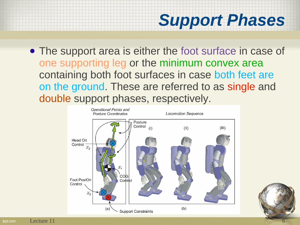
● The support area is either the foot surface in case of one supporting leg or the minimum convex area containing both foot surfaces in case both feet are on the ground. These are referred to as single and double support phases, respectively.

Lecture 11 7

Walking Speed

● Also, walking speed must be low so that inertial forces are negligible. This type of walking requires

large feet,

strong ankle joints● and can achieve only slow walking speeds.

Lecture 11 8

Simple Model of Walking

● Inverted Pendulum Model

● Influence of the Dynamics

● Center of Mass

● Center of Pressure

Lecture 11 9

Center of Mass I

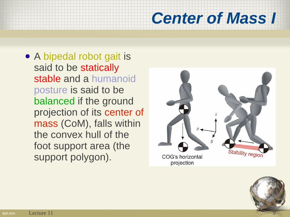
● A bipedal robot gait is said to be statically stable and a humanoid posture is said to be balanced if the ground projection of its center of mass (CoM), falls within the convex hull of the foot support area (the support polygon).

Lecture 11 10

Center of Mass II

● The center of mass is calculated according to its distance-weighted average location of the individual mass particles in the robot

● where Rmi

is the location of the mass particle ii, and MMii

is the mass of particle ii

CoM=∑ Rmi⋅M i

∑ M i

Lecture 11 11

Center of Pressure I

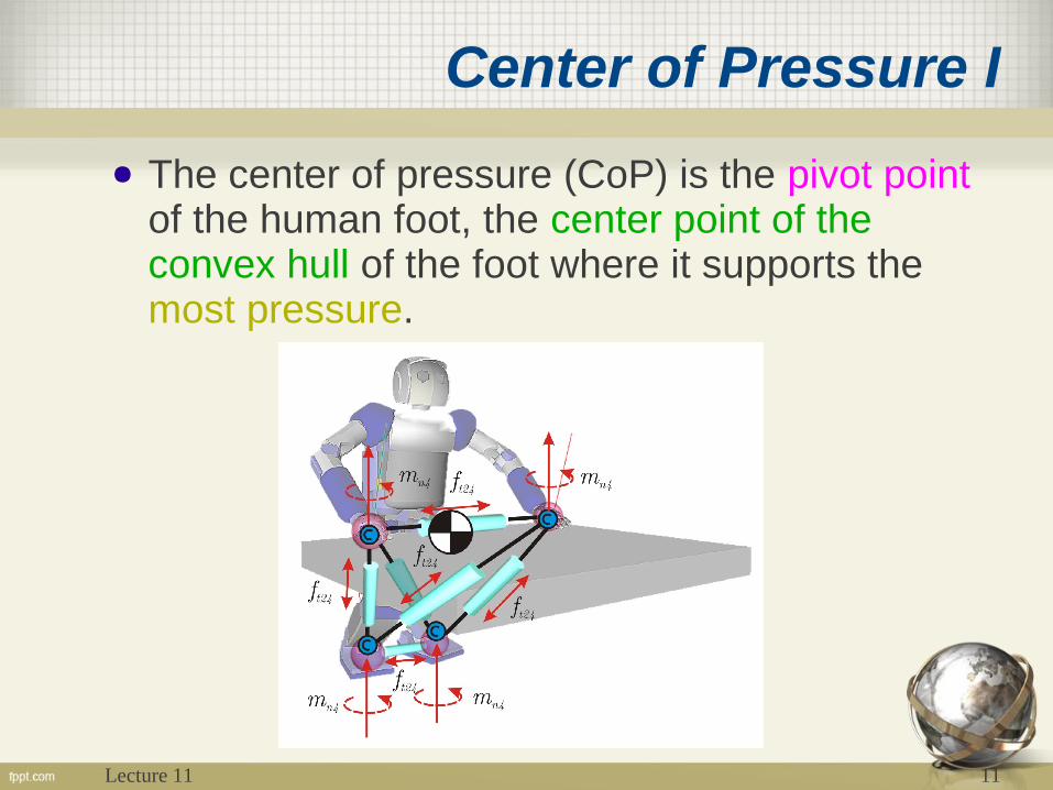
● The center of pressure (CoP) is the pivot point of the human foot, the center point of the convex hull of the foot where it supports the most pressure.

Lecture 11 12

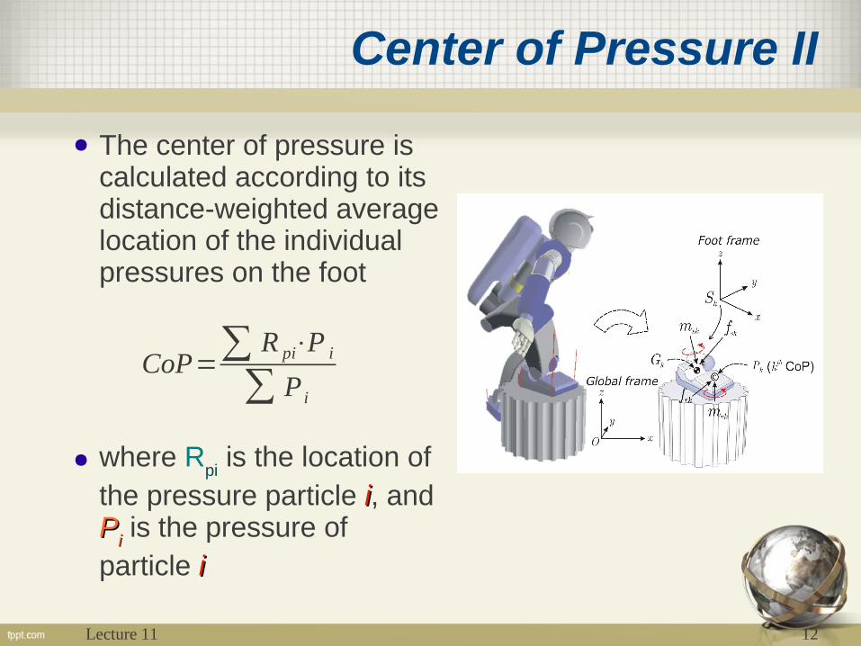
Center of Pressure II

● The center of pressure is calculated according to its distance-weighted average location of the individual pressures on the foot

● where Rpi is the location of

the pressure particle ii, and PPii

is the pressure of particle ii

CoP=∑ R pi⋅P i

∑ P i

Lecture 11 13

Inverted Pendulum Model

● The human walking motion shows some similarities with the inverted pendulum mechanics.

● The pendulum pivot point is placed approximately at the center of pressure on the foot. The pendulum mass is placed approximately at the center of mass.

Lecture 11 14

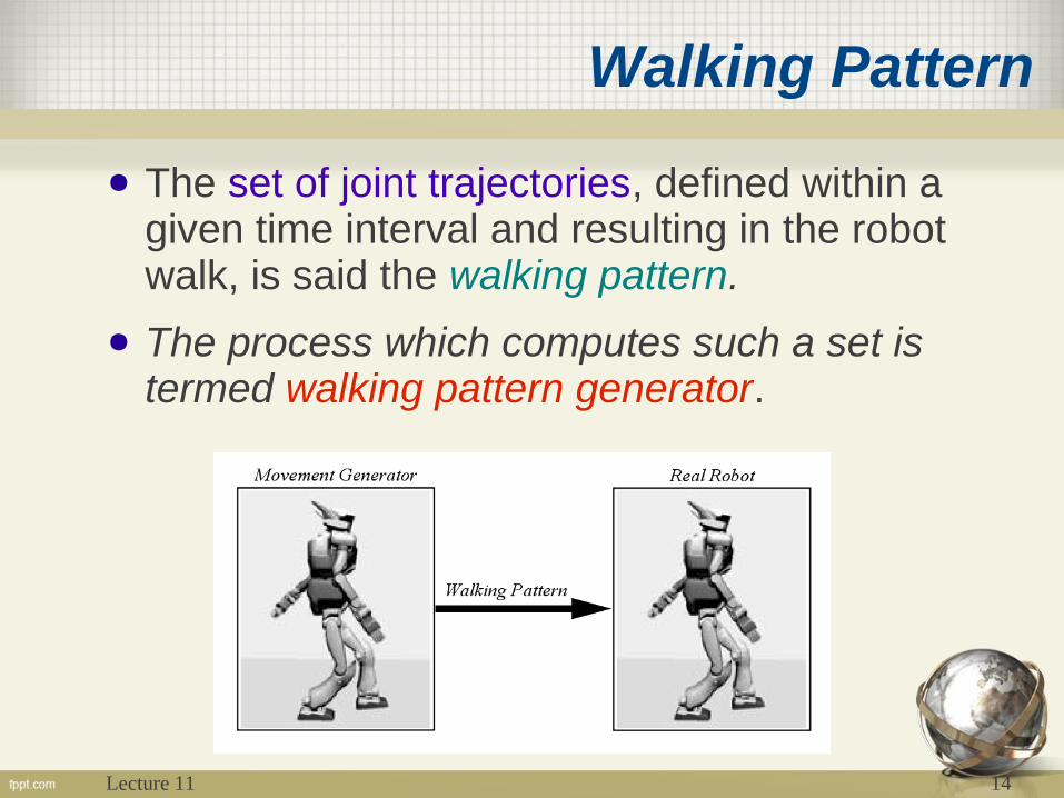
Walking Pattern

● The set of joint trajectories, defined within a given time interval and resulting in the robot walk, is said the walking pattern.

● The process which computes such a set is termed walking pattern generator.

Lecture 11 15

Model Hypothesis

● The dynamical behavior of a walking bipedal robot assumes

it is a point-reduced device concentrated on its centre of mass,

its legs have no mass and its feet are connected to the plain surface with spherical links,

its movement is only referred to either a front/rear displacement or up/down, namely, any lateral movement is neglected.

● In other words we consider the robot movement constrained on the so called sagittal plane

Lecture 11 16

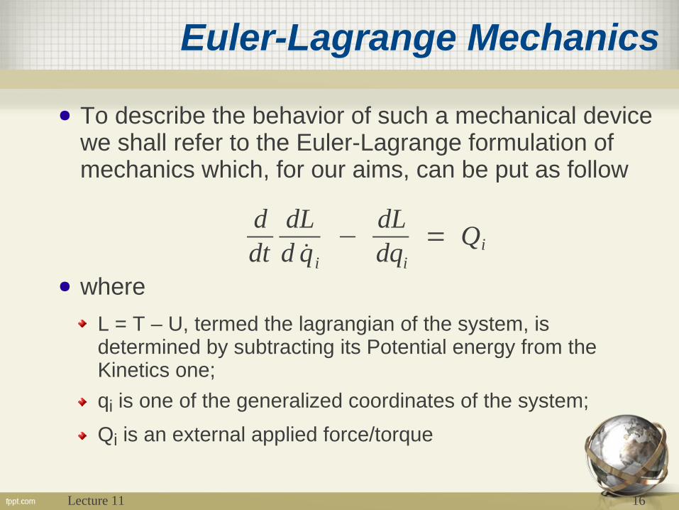
Euler-Lagrange Mechanics

● To describe the behavior of such a mechanical device we shall refer to the Euler-Lagrange formulation of mechanics which, for our aims, can be put as follow

● where

L = T – U, termed the lagrangian of the system, is determined by subtracting its Potential energy from the Kinetics one;

qi is one of the generalized coordinates of the system;

Qi is an external applied force/torque

ddt

dLd q i

−dLdqi

= Qi

Lecture 11 17

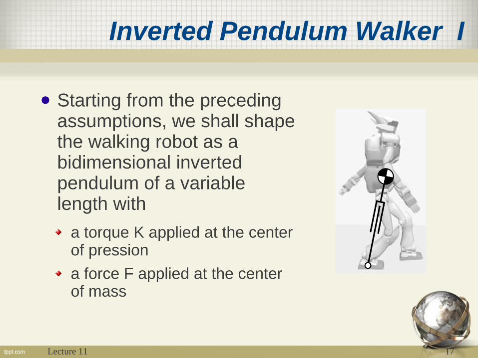
Inverted Pendulum Walker I

● Starting from the preceding assumptions, we shall shape the walking robot as a bidimensional inverted pendulum of a variable length with

a torque K applied at the center of pression

a force F applied at the center of mass

Lecture 11 18

Inverted Pendulum Walker II

● The lagrangian L of the simplified bipedal robot requires to determine both the Kinetics Energy

● and the Potential Energy

● so that we have

T=m2

r2r2

2

U=mg r cos

L=m2

r2r

2

2 − mg r cos

Lecture 11 19

Dynamic of the Pendulum

● The dynamics of the pendulum can be easily derived using the Euler-Lagrangian method:

for the coordinate r we have

whereas the coordinate yields to

ddt

r2 −grsin=

Km

r−r 2gcos=

Fm

Lecture 11 20

Force-driven Behaviors

● Since the leg structure prevents the application of an high torque at the ankle, we shall assume K = 0 so that only the force F at the hip remains active. Let us discuss the following ones:

free fall, if we assume no active force F;

fixed length leg, when the leg maintains a constant length

gravitational, when all the gravitational force acts on the hip;

fixed height, if the center of mass is kept at the same height during the motion.

Lecture 11 21

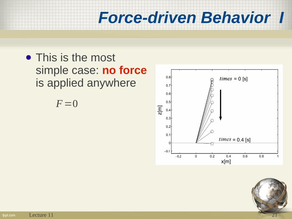
Force-driven Behavior I

● This is the most simple case: no force is applied anywhere

F=0

Lecture 11 22

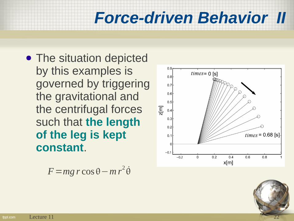
Force-driven Behavior II

● The situation depicted by this examples is governed by triggering the gravitational and the centrifugal forces such that the length of the leg is kept constant.

F=mg r cos−mr2

Lecture 11 23

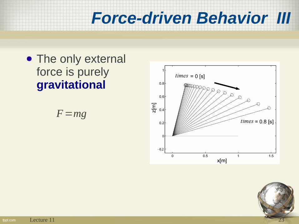
Force-driven Behavior III

● The only external force is purely gravitational

F=mg

Lecture 11 24

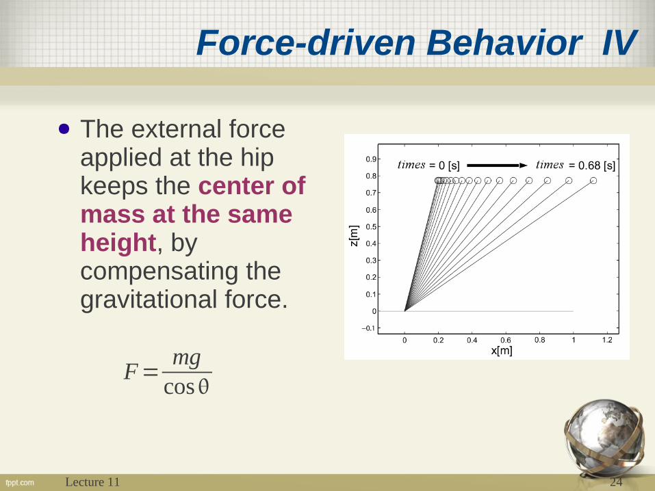
Force-driven Behavior IV

● The external force applied at the hip keeps the center of mass at the same height, by compensating the gravitational force.

F=mg

cos

Lecture 11 25

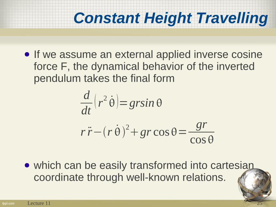
Constant Height Travelling

● If we assume an external applied inverse cosine force F, the dynamical behavior of the inverted pendulum takes the final form

● which can be easily transformed into cartesian coordinate through well-known relations.

ddt

r2 =grsin

r r−r 2gr cos=

grcos

Lecture 11 26

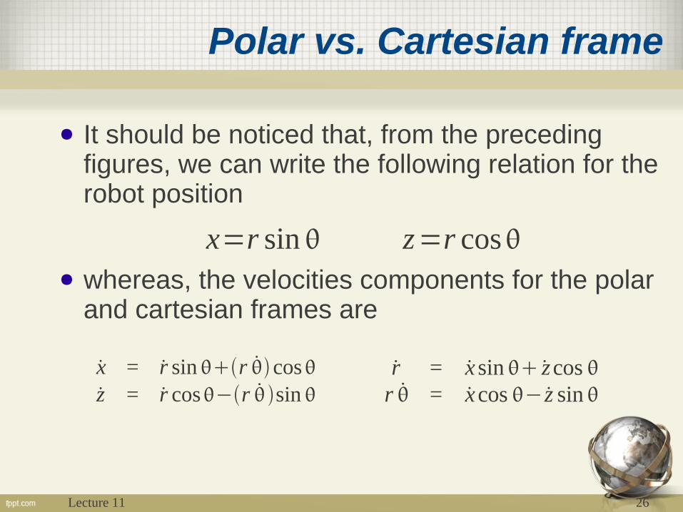
Polar vs. Cartesian frame

● It should be noticed that, from the preceding figures, we can write the following relation for the robot position

● whereas, the velocities components for the polar and cartesian frames are

x=r sin z=r cos

x = r sinr cosz = r cos−r sin

r = x sin zcos r = xcos − z sin

Lecture 11 27

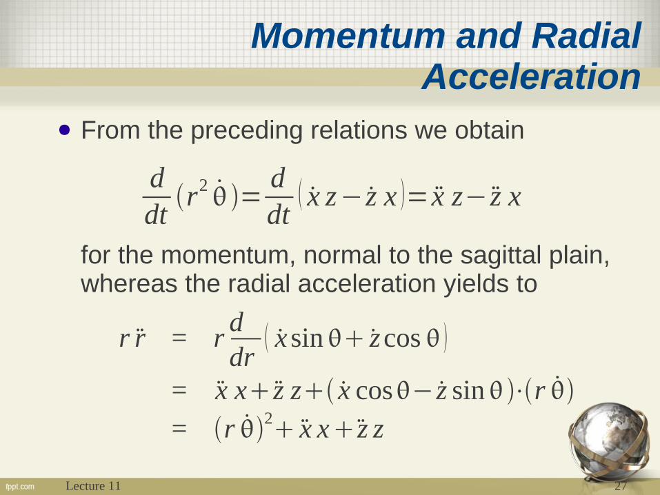
Momentum and Radial Acceleration

● From the preceding relations we obtain

for the momentum, normal to the sagittal plain, whereas the radial acceleration yields to

ddt

r2 =

ddt

x z− z x = x z− z x

r r = rddr

x sin zcos

= x x z z x cos− z sin⋅r

= r 2 x x z z

Lecture 11 28

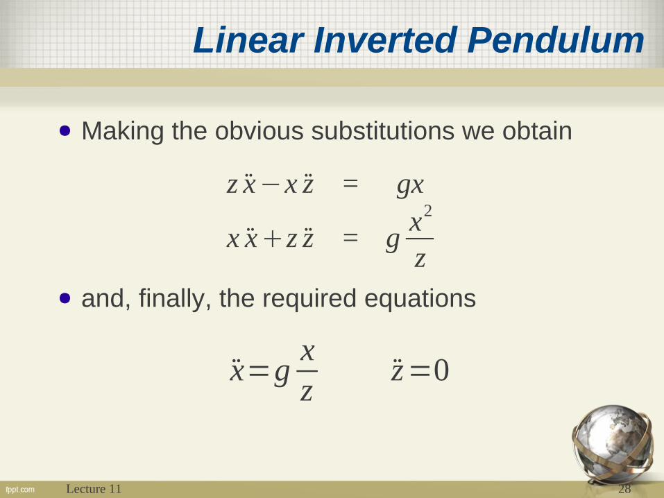
Linear Inverted Pendulum

● Making the obvious substitutions we obtain

● and, finally, the required equations

z x−x z = gx

x xz z = gx2

z

x=gxz

z=0

Lecture 11 29

LIP Behavior

● The situation is depicted in the figure. The explicit behavior can be easily written as follow

● where x0, u0 and l are given initial conditions and

c is defined as follow

x t = x0 cosh t c

cu0 sinht c

z t = l

c= lg

Lecture 11 30

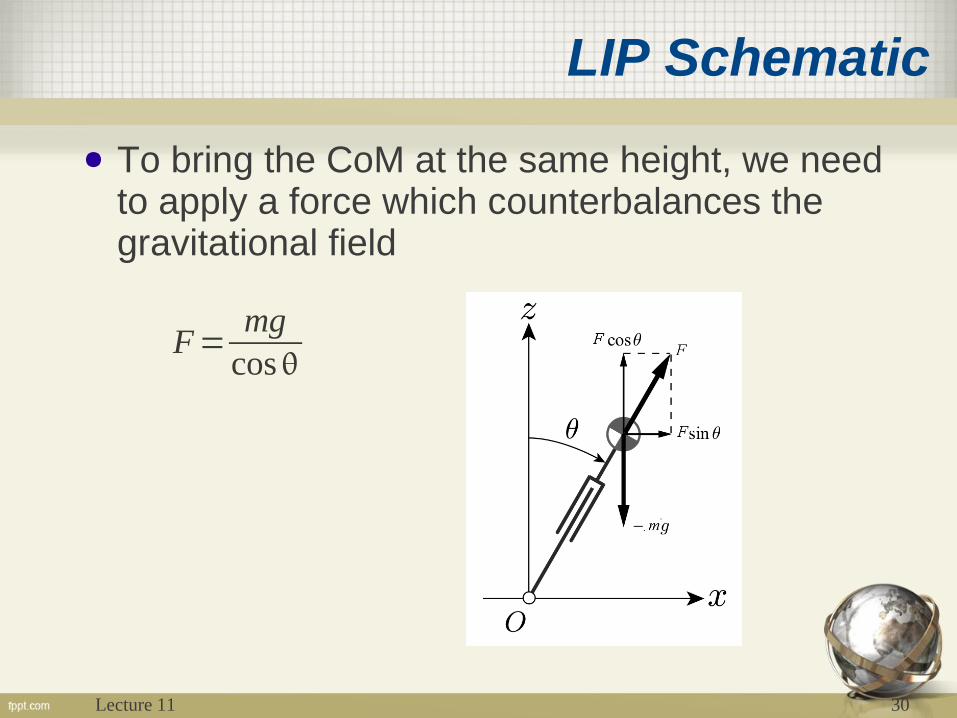
LIP Schematic

● To bring the CoM at the same height, we need to apply a force which counterbalances the gravitational field

F=mg

cos

Lecture 11 31

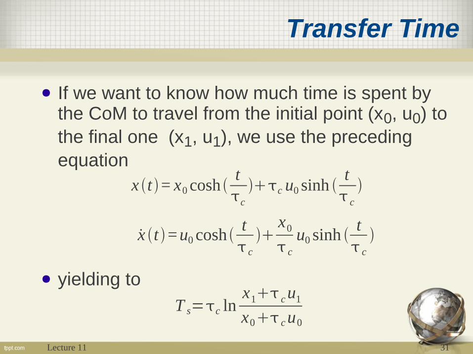
Transfer Time

● If we want to know how much time is spent by the CoM to travel from the initial point (x0, u0) to the final one (x1, u1), we use the preceding equation

● yielding to

x t = x0 cosh tc

c u0 sinh t c

x t =u0 cosh t c

x0

c

u0 sinh t c

T s=c lnx1 cu1

x0 cu0

Lecture 11 32

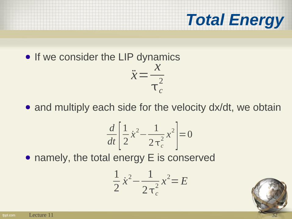
Total Energy

● If we consider the LIP dynamics

● and multiply each side for the velocity dx/dt, we obtain

● namely, the total energy E is conserved

x=x

c2

ddt [ 1

2x2

−1

2c2 x2]=0

12

x2−

1

2c2 x2

=E

Lecture 11 33

Equilibrium Point I

● The pendulum has an equilibrium point in the straight up position and will accelerate in the direction of whichever side it is on.

● The further the mass is from the vertical, the faster it will accelerate.

● Remember that there is no torque at the pivot point.

Lecture 11 34

Equilibrium Point II

● Suppose the mass is travelling from left to right.

● If the mass is on the left-hand side, it will slow down towards the vertical.

● If the mass has passed the vertical, it will accelerate to its right.

● At this point the system is converting kinetic energy into gravitational energy when it travels from left to vertical and convert it back into kinetic energy from the vertical to the right.

Lecture 11 35

Support Leg Exchange

● The LIP movement is determined by the given initial conditions. Thus, to modify this behavior we need to change the initial conditions, namely, the time interval through which the support foot is changed.

Lecture 11 36

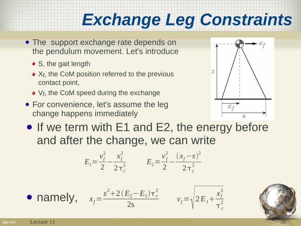
Exchange Leg Constraints● The support exchange rate depends on

the pendulum movement. Let's introduce

S, the gait length

Xf, the CoM position referred to the previous contact point,

Vf, the CoM speed during the exchange

● For convenience, let's assume the leg change happens immediately

● If we term with E1 and E2, the energy before and after the change, we can write

● namely,

E1=v f

2

2−

x f2

2c2 E2=

v f2

2−

x f −s 2

2 c2

x f=s2

2 E2−E1 c2

2sv f =2E1

x f2

c2

Lecture 11 37

Gait Pattern: phases

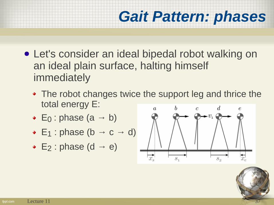
● Let's consider an ideal bipedal robot walking on an ideal plain surface, halting himself immediately

The robot changes twice the support leg and thrice the total energy E:

E0 : phase (a → b)

E1 : phase (b → c → d)

E2 : phase (d → e)

Lecture 11 38

Gait Pattern: energy

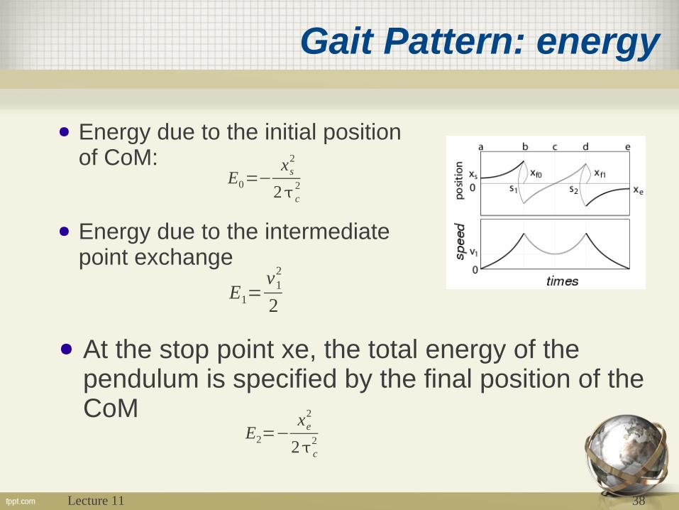
● Energy due to the initial position of CoM:

● Energy due to the intermediate point exchange

● At the stop point xe, the total energy of the pendulum is specified by the final position of the CoM

E0=−xs

2

2 c2

E1=v1

2

2

E2=−xe

2

2 c2

Lecture 11 39

Linear Actuator Pendulum Model

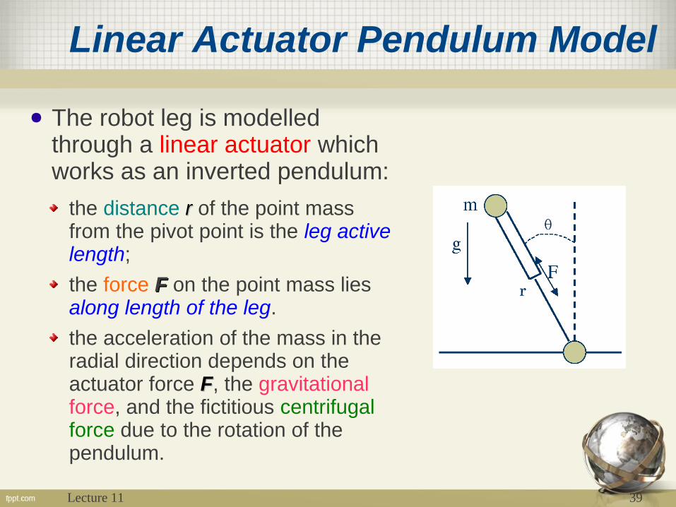
● The robot leg is modelled through a linear actuator which works as an inverted pendulum:

the distance rr of the point mass from the pivot point is the leg active length;

the force FF on the point mass lies along length of the leg.

the acceleration of the mass in the radial direction depends on the actuator force FF, the gravitational force, and the fictitious centrifugal force due to the rotation of the pendulum.

Lecture 11 40

Linear Actuator Dynamics

● If we want to understand qualitatively how the linear actuator works, let's ssume the mass of the pendulum is travelling from left to right:

With the actuator pulling the mass, the rotation motion will accelerate.

Extending the mass will decelerate the speed.

● This is the same as sitting on a spinning chair where the pivot point is underneath the chair, when opening the arms during spinning, the rotation will slow down, while closing up the arms will increase the rotational speed.

Lecture 11 41

Multi Joint Similarities

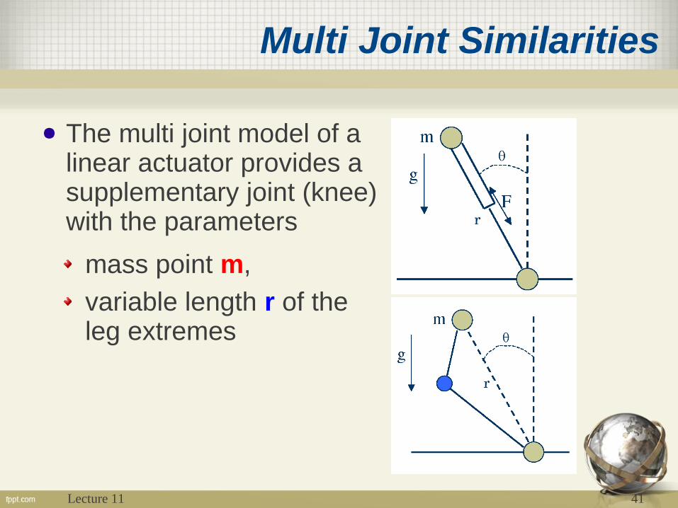
● The multi joint model of a linear actuator provides a supplementary joint (knee) with the parameters

mass point m,

variable length r of the leg extremes

Lecture 11 42

Multi Joint Model I

● This model shares some characteristics with the linear actuator model, but it is implemented with a different mechanism.

● In orderto transform a linear actuator model into a multi joint pendulum model, we have to show that both dynamics are identical.

● We illustrate the similarities, by using a two degrees of freedom (DOF) multi joint model with the parameters mass point m, length l of the leg.

Lecture 11 43

Multi Joint Model II

● With a different mechanical design, to obtain the same parameters we have to use inverse kinematics to calculate the angles for each individual joint.

● The only difference between the two models is the force gain from the actuator, for linear actuator model it is a linear force.

● This model has a torque generated by the knee servo but it has a minor influence.

Lecture 11 44

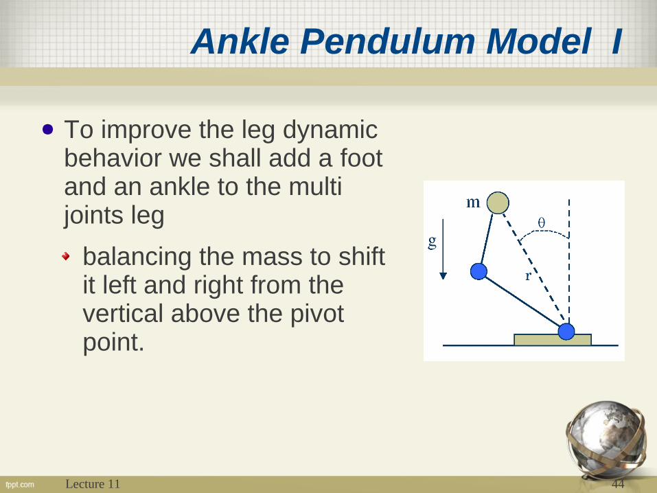
Ankle Pendulum Model I

● To improve the leg dynamic behavior we shall add a foot and an ankle to the multi joints leg

balancing the mass to shift it left and right from the vertical above the pivot point.

Lecture 11 45

Ankle Pendulum Model II

● Controlling the speed of the rotation motionspeed of the rotation motion of the inverted pendulum by adjusting the length adjusting the length of the legof the leg is not a well-balanced system.

● Adding a foot and an ankle brings many benefits:

it yields to a larger supporting area (convex hull of the feet) for the center of mass to stay below when traveling.it also helps to control the speed of the pendulum and leads to a more stable system.

Lecture 11 46

Controlling the Joints Torque

● Balancing the mass is made by shifting it left and right from the vertical above the pivot point.

● The pivot point of a human is the center of pressure (CoP), thus

if the CoP is left of the CoM then the mass point will accelerate to the right;if the CoP is right of the CoM then the mass point will accelerate to the left.

● By controlling the joints torque, we can arbitrarily control the location of the center of pressure.