BioOne sees sustainable scholarly publishing as an inherently collaborative enterprise connecting authors, nonprofitpublishers, academic institutions, research libraries, and research funders in the common goal of maximizing access tocritical research.

Northern Goshawk Monitoring In the Western Great LakesBioregionAuthor(s) :Jason E. Bruggeman, David E. Andersen, and James E. WoodfordSource: Journal of Raptor Research, 45(4):290-303. 2011.Published By: The Raptor Research FoundationDOI:URL: http://www.bioone.org/doi/full/10.3356/JRR-10-52.1

BioOne (www.bioone.org) is a a nonprofit, online aggregation of core research in thebiological, ecological, and environmental sciences. BioOne provides a sustainableonline platform for over 170 journals and books published by nonprofit societies,associations, museums, institutions, and presses.

Your use of this PDF, the BioOne Web site, and all posted and associated contentindicates your acceptance of BioOne’s Terms of Use, available at www.bioone.org/page/terms_of_use.

Usage of BioOne content is strictly limited to personal, educational, and non-commercial use. Commercial inquiries or rights and permissions requests should bedirected to the individual publisher as copyright holder.

NORTHERN GOSHAWK MONITORING IN THE WESTERNGREAT LAKES BIOREGION

JASON E. BRUGGEMAN1

Minnesota Cooperative Fish and Wildlife Research Unit, Department of Fisheries, Wildlife, and ConservationBiology, University of Minnesota, St. Paul, MN 55108 U.S.A.

DAVID E. ANDERSENU.S. Geological Survey, Minnesota Cooperative Fish and Wildlife Research Unit, University of Minnesota,

St. Paul, MN 55108 U.S.A.

JAMES E. WOODFORDWisconsin Department of Natural Resources, Endangered Resources Program, Rhinelander, WI 54501 U.S.A.

ABSTRACT.—Uncertainties about factors affecting Northern Goshawk (Accipiter gentilis) ecology and thestatus of populations have added to the challenge of managing this species. To address data needs fordetermining the status of goshawk populations, Hargis and Woodbridge (2006) developed a bioregionalmonitoring protocol based on estimating occupancy. The goal of our study was to implement this protocoland collect data to determine goshawk population status in the western Great Lakes (WGL) bioregion,which encompasses portions of Minnesota, Wisconsin, and Michigan, and is a mixture of private and publicproperty. We used 366 goshawk nest locations obtained between 1979 and 2006 throughout the WGLbioregion to develop a model of landscape use consisting of forest canopy cover and land-cover covariates.We then used the model to develop a stratified sampling design for selecting 600-ha Primary SamplingUnits (PSUs) to survey for goshawks. Project collaborators surveyed 86 PSUs for goshawk presence usingbroadcasted calls twice between mid-May and mid-August 2008, and recorded 30 goshawk detections in 21different PSUs. Seventy-four percent of detections occurred at call stations with canopy closure .75%.Goshawk detection probabilities were 0.549 6 0.118 (standard error) for the first visit to PSUs and 0.750 6

0.126 for the second visit. We estimated the proportion of PSUs occupied by goshawks as 0.266 6 0.047,which corresponded to 5184 6 914 PSUs occupied by goshawks in our study area and suggested thatgoshawks are widely, but sparsely, distributed throughout the WGL bioregion.

KEY WORDS: Northern Goshawk; Accipiter gentilis; occupancy; population monitoring; raptors; stratified sampling;surveys; western Great Lakes bioregion.

MONITOREO DE ACCIPITER GENTILIS EN LA BIOREGION DEL OESTE DE LOS GRANDES LAGOS

RESUMEN.—La incertidumbre acerca de los factores que afectan la ecologıa de Accipiter gentilis y el estado desus poblaciones se han anadido al reto del manejo de esta especie. Para hacer frente a las necesidades dedatos para determinar el estado de las poblaciones de A. gentilis, Hargis y Woodbridge (2006) desarrollaronun protocolo de monitoreo bioregional basado en estimados de ocupacion. El objetivo de nuestro estudiofue la implementacion de este protocolo y colectar datos para determinar el estado de la poblacion de A.gentilis en la bioregion del oeste de los Grandes Lagos (OGL), que abarca partes de Minnesota, Wisconsin yMichigan, y es una mezcla de propiedades publicas y privadas. Utilizamos 366 sitios de nidos de A. gentilisobtenidos entre 1979 y 2006 en toda la bioregion del OGL para desarrollar un modelo de uso del paisajeque consistio en covariables de la cobertura de dosel de bosque y cobertura de suelo. A continuacion,utilizamos el modelo para desarrollar un diseno de muestreo estratificado para seleccionar 600 ha deUnidades Primarias de Muestreo (UPM) para muestrear individuos de A. gentilis. Los colaboradores delproyecto muestrearon 86 UPM’s para determinar la presencia de estos halcones utilizando emision dellamadas grabadas entre mediados de mayo y mediados de agosto de 2008, y registraron 30 detecciones de

1 Present address: Beartooth Wildlife Research, LLC, Farmington, MN 55024, U.S.A.; email address: jbruggeman@frontiernet.net

J. Raptor Res. 45(4):290–303

E 2011 The Raptor Research Foundation, Inc.

290

A. gentilis en 21 UPM’s diferentes. Setenta y cuatro por ciento de las detecciones se produjeron en lasestaciones de llamada con cobertura de dosel de .75%. La probabilidad de deteccion de los halcones fuede 0.549 6 0.118 (error estandar) para la primera visita a una UPM y de 0.750 6 0.126 para la segundavisita. Estimamos la proporcion de PCU’s ocupadas por A. gentilis en 0.266 6 0.047, que correspondio a5.184 6 914 PSU ocupadas por A. gentilis en nuestra area de estudio, y sugirio que los individuos de A.gentilis se distribuyen ampliamente pero de forma dispersa por toda la bioregion del OGL.

[Traduccion del equipo editorial]

The challenge of managing forest resources forNorthern Goshawk (Accipiter gentilis; hereafter, ‘‘gos-hawk’’) populations in North America has involvedmaintaining suitable nesting and foraging habitatwhile simultaneously allowing for timber harvestand other activities (Squires and Kennedy 2006).Goshawks have been associated with mature forestsbecause of their observed use of stands with relative-ly large trees and high canopy closure (Squires andReynolds 1997, Boal et al. 2005). However, muchregional variation exists in tree species and sizesused for nests (Siders and Kennedy 1994, Squiresand Ruggiero 1996, Boal et al. 2006). Goshawk dietsare diverse across their breeding range (Doyle andSmith 2001, Salafsky et al. 2005, Smithers et al.2005), and suitable foraging habitat for goshawksmay encompass a broader range of forest typesand structure than that for nests (Boal et al. 2005,Reynolds et al. 2008). Much of the literature ongoshawk nesting, foraging, movements, and demog-raphy has come from research in the southwesternand western United States (e.g., Andersen et al.2005, Fairhurst and Bechard 2005, Reynolds et al.2005, Wiens et al. 2006b), and greater uncertaintyabout their ecology remains elsewhere in NorthAmerica.

Knowledge of large-scale, regional trends in gos-hawk populations is needed to evaluate whetherpopulations are decreasing, stationary, or increasing(Andersen et al. 2005). To achieve this, Woodbridgeand Hargis (2006) developed a goshawk monitoringprotocol for use in designing monitoring plans for 10‘‘bioregions’’ throughout the country. The objec-tives of bioregional monitoring were to: (1) estimatethe frequency of occurrence of goshawks within eachbioregion; (2) assess changes in the frequency ofoccurrence over time, and (3) determine whetherany changes in the frequency of occurrence wererelated to habitat change (Hargis and Woodbridge2006). A regional scale for goshawk monitoring wassuggested because surveying smaller land units suchas individual national forest lands is problematic ow-ing to ecological and sampling reasons (Hargis andWoodbridge 2006). Goshawks are highly mobile and

the interbreeding population spans a regional scale.Obtaining an adequate sample size within one forestto determine a change in population abundancewith sufficient power is costly (Hargis and Wood-bridge 2006). The goshawk monitoring protocol(Hargis and Woodbridge 2006) addresses study de-sign recommendations of Pollock et al. (2002) byaffording inference to the entire sampled portionof the bioregion and estimating detection probabili-ties using double sampling.

Information on goshawk ecology is limited and thepopulation status of the species is unknown withinthe western Great Lakes (WGL) bioregion that en-compasses portions of Minnesota, Wisconsin, andMichigan (Boal et al. 2006). The goals of our studyincluded addressing data needs for determining gos-hawk population status in the WGL bioregion usingthe goshawk monitoring protocol of Hargis andWoodbridge (2006) and concurrently collecting hab-itat-use information. We first used existing goshawknest location data from the WGL bioregion to devel-op a model of goshawk landscape use consisting ofhabitat attribute covariates derived from GeographicInformation System (GIS) layers. We then used themodel to assist in developing a stratified randomsampling design for selecting sampling units forthe bioregional survey. Finally, we completed thebioregional survey in 2008 and estimated goshawkoccupancy and detection probabilities for the por-tion of the bioregion that we surveyed. This workprovides the first estimate of goshawk occupancyfor the WGL population and offers insights intothe potential for monitoring goshawks and other rap-tors in other regions of North America.

METHODS

Study Area. The WGL bioregion consists of landsin northeastern and north-central Minnesota,northern Wisconsin, and northern Michigan(Woodbridge and Hargis 2006) and encompassesthe approximate goshawk breeding range basedon historical locations of nests (Fig. 1). Becausefunding limitations precluded surveying the entirebreeding range, we delineated our study area based

DECEMBER 2011 NORTHERN GOSHAWK MONITORING 291

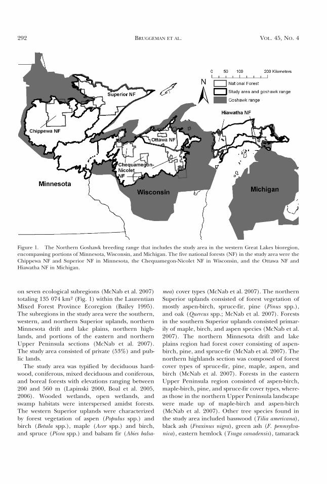
on seven ecological subregions (McNab et al. 2007)totaling 135 074 km2 (Fig. 1) within the LaurentianMixed Forest Province Ecoregion (Bailey 1995).The subregions in the study area were the southern,western, and northern Superior uplands, northernMinnesota drift and lake plains, northern high-lands, and portions of the eastern and northernUpper Peninsula sections (McNab et al. 2007).The study area consisted of private (53%) and pub-lic lands.

The study area was typified by deciduous hard-wood, coniferous, mixed deciduous and coniferous,and boreal forests with elevations ranging between200 and 560 m (Lapinski 2000, Boal et al. 2005,2006). Wooded wetlands, open wetlands, andswamp habitats were interspersed amidst forests.The western Superior uplands were characterizedby forest vegetation of aspen (Populus spp.) andbirch (Betula spp.), maple (Acer spp.) and birch,and spruce (Picea spp.) and balsam fir (Abies balsa-

mea) cover types (McNab et al. 2007). The northernSuperior uplands consisted of forest vegetation ofmostly aspen-birch, spruce-fir, pine (Pinus spp.),and oak (Quercus spp.; McNab et al. 2007). Forestsin the southern Superior uplands consisted primar-ily of maple, birch, and aspen species (McNab et al.2007). The northern Minnesota drift and lakeplains region had forest cover consisting of aspen-birch, pine, and spruce-fir (McNab et al. 2007). Thenorthern highlands section was composed of forestcover types of spruce-fir, pine, maple, aspen, andbirch (McNab et al. 2007). Forests in the easternUpper Peninsula region consisted of aspen-birch,maple-birch, pine, and spruce-fir cover types, where-as those in the northern Upper Peninsula landscapewere made up of maple-birch and aspen-birch(McNab et al. 2007). Other tree species found inthe study area included basswood (Tilia americana),black ash (Fraxinus nigra), green ash (F. pennsylva-nica), eastern hemlock (Tsuga canadensis), tamarack

Figure 1. The Northern Goshawk breeding range that includes the study area in the western Great Lakes bioregion,encompassing portions of Minnesota, Wisconsin, and Michigan. The five national forests (NF) in the study area were theChippewa NF and Superior NF in Minnesota, the Chequamegon-Nicolet NF in Wisconsin, and the Ottawa NF andHiawatha NF in Michigan.

292 BRUGGEMAN ET AL. VOL. 45, NO. 4

(Larix laricina), and northern white-cedar (Thujaoccidentalis).

Development of a Goshawk Landscape-useModel and Stratified Random Sampling Design.We placed a grid of 600-ha squares called PrimarySampling Units (PSUs; Hargis and Woodbridge2006) over the goshawk breeding range in theWGL bioregion, resulting in a total of 49 146 PSUs.The size of the PSU was defined in the monitoringprotocol (Woodbridge and Hargis 2006), and ap-proximated the size of one goshawk territory basedon data primarily from western North America. Weused location data from 366 goshawk nests obtainedfrom 1979 to 2006 in the WGL and GIS layers todevelop a model of goshawk landscape use to assistwith designing a stratified random sampling proto-col. Using GIS techniques, we centered each nestwithin a 600-ha square, which corresponded to thePSU size that would later be used for surveying forgoshawk presence. Within each square, we random-ly placed 120 points that corresponded to the 120call stations to be visited during surveys (Wood-bridge and Hargis 2006). For each of the 366 nestlocations, we randomly distributed 20 600-hasquares (i.e., 7320 squares in total), each containing120 randomly located points, throughout the entiregoshawk range to assess habitat that was available,but not known to be used for nesting. We used twodifferent GIS data layers to determine habitat attri-bute covariates for each 600-ha square. We used theNational Land Cover Database (NLCD) land-coverlayer with 30-m 3 30-m resolution (Homer et al.2004) to classify the land-cover type of each randompoint and calculated seven covariates with each de-fined as the percent of each 600-ha square consist-ing of different land covers (Appendix, Table A1;Bruggeman et al. 2009). The land-cover layer pro-vided a categorical cover classification for each 30-m3 30-m pixel. We used a U.S. Geological Survey(USGS) forest canopy-cover layer (Huang et al.2003), which has been assessed and used in otherstudies (Walton et al. 2008, Sander et al. 2010), todetermine the percent canopy cover at each ran-dom point and calculated 13 different canopy covercovariates (Appendix, Table A2; Bruggeman et al.2009). The forest canopy-cover layer provided a val-ue of canopy cover in increments of one percent foreach 30-m 3 30-m pixel. The forest canopy-coverlayer was developed at a spatial resolution of 30 mbased on empirical relationships between tree can-opy density and Landsat 7 Enhanced ThematicMapper Plus data, with 1-m digital orthophoto

quadrangles used to derive reference tree canopydensity data to calibrate relationships between can-opy density and Landsat data (Huang et al. 2001,2003).

We used these data to develop a model predictinggoshawk landscape use. We assigned squares con-sisting of goshawk locations a ‘‘1’’ (366 squares)and randomly placed squares a ‘‘0’’ (7320 squares)as a binary response variable. We systematically de-veloped 172 logistic regression use/availability mod-els (Hosmer and Lemeshow 2000, Manly et al. 2002)consisting of combinations of the 13 canopy-coverand seven land-cover covariates (Bruggeman et al.2009). We used PROC LOGISTIC in SAS v9.1 (Alli-son 1999) to fit models and estimate covariate coef-ficients. For each model we calculated an Akaike’sInformation Criterion (AIC) value and an Akaikeweight (w), and then ranked and selected top mod-els using DAIC values (Burnham and Anderson2002).

We used the best-supported model to estimatethe probability of goshawk landscape use at eachof the 366 nest locations and examined a distribu-tion of the probability values to help define rangesfor primary, secondary, and non-habitat classifica-tions (Bruggeman et al. 2009). Probability of gos-hawk landscape use ranged between 0.001 and0.567 [mean 5 0.111; standard deviation (SD) 5

0.082; standard error (SE) 5 0.004]. We definedprimary goshawk habitat to have a probability ofuse $0.111, secondary habitat to have a probabilitybetween 0.028 and 0.111 (i.e., between the mean – 1SD and the mean), and non-habitat to have proba-bility ,0.028. Within each of the 49 146 PSUs (i.e.,the WGL bioregion), we randomly placed 120 pointsand calculated the 20 covariates used in the model-ing. We used the best-supported model to predictthe probability of goshawk landscape use in eachPSU and classified 6860 PSUs as primary habitat,25 750 as secondary habitat, and 16 536 as non-hab-itat.

We used GIS layers of federal and state land own-ership, and major roads for Michigan, Minnesota,and Wisconsin to determine PSU accessibility. Wecalculated the nearest Euclidean distance from thecentroid of each PSU to a road (paved or ForestService) and the proportion of each PSU that con-sisted of project collaborators’ lands (e.g., nationalforests and parks; state forests and parks; tribal or-ganizations). The proportion of each PSU that wascomposed of project collaborators’ lands ranged be-tween 0.0 and 1.0 (mean 5 0.533; SE 5 0.002), and

DECEMBER 2011 NORTHERN GOSHAWK MONITORING 293

the distance of each PSU to the nearest road rangedbetween 0 km and 48 km (mean 5 5.00; SE 5 0.02).We classified any PSU that had either a proportionof collaborator land ownership ,0.533 or a distanceto road .10 km (i.e., mean + 1 SD) as difficultaccess. We classified easy access PSUs as only thosethat had both a proportion of collaborator landownership $0.533 and a distance to road #10 km.Within our study area consisting of the seven subre-gions there were 19 506 PSUs distributed amongfour strata as follows: (1) 1293 in primary habitat/difficult access; (2) 3564 in primary habitat/easyaccess; (3) 7047 in secondary habitat/difficult ac-cess, and (4) 7602 in secondary habitat/easy access(Fig. 2a). There were an additional 4483 PSUs clas-sified as non-habitat that were removed from thesampling universe. We used an optimal sample-sizeallocation algorithm to determine the number ofPSUs per stratum that could be surveyed given proj-ect funding (Hargis and Woodbridge 2006). Oursample of 86 PSUs consisted of seven in the primaryhabitat/difficult access stratum, 27 in primary hab-itat/easy access, 22 in secondary habitat/difficultaccess, and 30 in secondary habitat/easy access(Fig. 2b).

Northern Goshawk Surveys and HabitatData Collection. Goshawk surveys were conductedunder the University of Minnesota Institutional An-imal Care and Use Committee, approved protocolnumber 0806A35181. Between mid-May and mid-August 2008, surveyors systematically surveyed the86 PSUs in our sample (Fig. 2b) for goshawk pres-ence or absence in accordance with the NorthernGoshawk Inventory and Monitoring TechnicalGuide (Woodbridge and Hargis 2006). Each PSUwas surveyed by a field crew of two surveyors apiecewith crews consisting of biologists from the U.S.Forest Service, Minnesota Department of NaturalResources, Wisconsin Department of Natural Re-sources, Michigan Natural Features Inventory, andUniversity of Minnesota. Each 600-ha PSU con-tained 120 call stations located on 10 transectsspaced 250 m apart (Woodbridge and Hargis2006). Along each transect were 12 call stations sep-arated by 200 m, with adjacent transect call stationsoffset by 100 m from north to south to maximizecoverage (Woodbridge and Hargis 2006). Trainedsurveyors used vocal and/or visual responses by gos-hawks to call broadcasts (Kennedy and Stahlecker1993) and sightings of recent goshawk activity (e.g.,occupied nests, freshly molted feathers, pluckingposts and excreta) to determine goshawk presence

at and between call stations (Woodbridge and Har-gis 2006). Call stations were surveyed until either agoshawk was detected or all 120 stations in the PSUwere surveyed (Woodbridge and Hargis 2006). Ifsurveyors detected a goshawk, then the survey forthe PSU was complete (Woodbridge and Hargis2006). Two visits per PSU were scheduled with thefirst survey conducted between mid-May throughlate June (i.e., the nestling period) and the secondbetween July and mid-August (i.e., the fledglingperiod). Using either a Western Rivers Predation(Western Rivers, Lexington, Tennessee, U.S.A.) orFOX PRO FX3 (FOX PRO, Inc., Lewistown, Penn-sylvania, U.S.A.) digital caller, surveyors broadcast agoshawk alarm call (Woodbridge and Hargis 2006)at a minimum of 95 dB at each station during thenestling period and alternated between the alarmcall and a juvenile food-begging call (Woodbridgeand Hargis 2006) at stations during the fledglingperiod. At each station, surveyors broadcast the callfor 10 sec, listened for a response for 30 sec, rotated120u, and repeated the call/listening sequence. Atotal of six calling sequences encompassing twocomplete 360u turns were made at each station. Ifa detection did not occur during the first visit, thena second visit was required. However, if a detectionoccurred during the first visit, then a second visitwas required only for a subsample of PSUs for thepurpose of calculating detection probabilities(Woodbridge and Hargis 2006).

Surveyors recorded habitat data at each call sta-tion surveyed for goshawks including the predomi-nant primary and secondary/conifer forest types,and principal structural stage within a 25-m radiusaround the station. The primary forest type was thedominant species, or multiple species, and was clas-sified as either deciduous or coniferous. A second-ary/conifer type was recorded only when a conifer-ous species, or multiple coniferous species, waspresent, but was not the dominant type. Deciduousforest types were categorized as: (1) aspen; (2) whitebirch (Betula papyrifera); (3) oak; (4) northern hard-wood (combinations of maple, oak, basswood, andash); (5) northern hardwood with yellow birch (Bet-ula alleghaniensis), or (6) swamp hardwood (mapleand black ash). Coniferous types were classified as:(1) white pine (Pinus strobus); (2) red pine (Pinusresinosa); (3) jack pine (Pinus banksiana); (4) hem-lock; (5) spruce and balsam fir, or (6) swamp coni-fer [combinations of black spruce (Picea mariana),tamarack, or northern white-cedar]. Surveyors alsorecorded if any of the pine species were part of a pine

294 BRUGGEMAN ET AL. VOL. 45, NO. 4

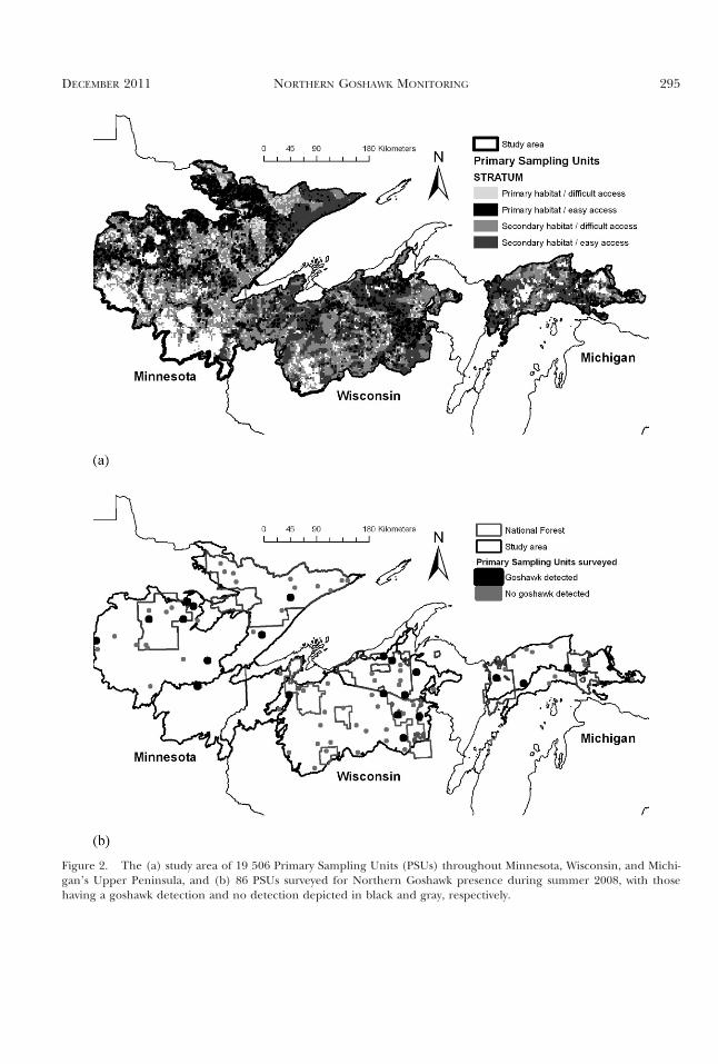
Figure 2. The (a) study area of 19 506 Primary Sampling Units (PSUs) throughout Minnesota, Wisconsin, and Michi-gan’s Upper Peninsula, and (b) 86 PSUs surveyed for Northern Goshawk presence during summer 2008, with thosehaving a goshawk detection and no detection depicted in black and gray, respectively.

DECEMBER 2011 NORTHERN GOSHAWK MONITORING 295

plantation. Surveyors classified stations that were sur-rounded by meadows, water, or developed land as‘‘non-forested.’’ At each station surveyors classifiedthe predominant structural stage into one of five cat-egories: (1) grass, forbs, shrubs, or seedlings; (2) sap-ling-pole with canopy closure ,75% (trees rangingbetween 2.5 cm and 23 cm diameter at breast height[dbh] size for softwoods; 2.5 cm and 28 cm for hard-woods); (3) sapling-pole with canopy closure .75%(trees ranging between 2.5 cm and 23 cm dbh size forsoftwoods; 2.5 cm and 28 cm for hardwoods); (4)late-successional with canopy closure ,75% (trees.23 cm dbh for softwoods; .28 cm dbh for hard-woods), and (5) late-successional with canopy closure.75% (trees .23 cm dbh for softwoods; .28 cm dbhfor hardwoods).

Estimation of Northern Goshawk Occupancy andDetection Probabilities. We used the 2008 surveyresults to estimate the number of PSUs occupiedby goshawks in our study area within the WGL bio-region. We used maximum likelihood techniques toestimate the proportion of PSUs occupied by gos-hawks (Pi) for each stratum (1 # i # 4), and theprobabilities of missing presence for visit numberone (q1) and visit number two (q2; Hargis andWoodbridge 2006). We calculated detection proba-bilities based on presence/absence data recordedfor the two visits to each PSU that resulted in oneof the following sequences: 00, 01, 10, 1*, or 11,where a ‘‘1’’ denotes presence and ‘‘0’’ an absence(Hargis and Woodbridge 2006). The 1* sequenceapplied to PSUs surveyed in visit number one andwhere a goshawk was detected, but not surveyedagain (Hargis and Woodbridge 2006). We estimatedstandard errors for each Pi using bootstrap methods(Efron and Tibshirani 1993). The sample size foreach stratum was the number of PSUs surveyed ineach stratum (ni) and we selected 1000 bootstrapsamples of size ni for each stratum using randomsampling with replacement. We calculated themean proportion of PSUs occupied by goshawksfrom the sample and the associated standard errorfrom the bootstrap sample (SEi). We then deter-mined the sample variance of the mean proportionof PSUs occupied by goshawks for each stratum assi

2 5 SEi2*ni. We used Pi, determined from maxi-

mum likelihood estimates, and si2, determined

from bootstrapping, in stratified random samplingequations (Thompson 2002) to estimate the totalnumber and proportion of PSUs in our study areaoccupied by goshawks and the associated variancefor each. Likewise, we estimated standard errors for

q1 and q2 using bootstrap methods (Efron and Tib-shirani 1993). The sample size for q1 was 17 because17 PSUs had detection sequences of 01 or 11 where-as the sample size for q2 was 12 because 12 PSUs hadsequences of 10 or 11. We selected 1000 bootstrapsamples of size 17 for q1 and 12 for q2 using randomsampling with replacement. We calculated the meandetection probabilities from each sample and theassociated standard error.

Power Analyses. We conducted power analyses(Cohen 1992) in R (R Development Core Team2008) to examine the ability to detect a change(i.e., increase or decrease) or decline in goshawkoccupancy in our study area with the next survey.Using the coefficient of variation (CV) of occupancydetermined from maximum likelihood and boot-strap standard error estimates, we examined howvarying the percent change in occupancy influ-enced the power to detect a change or decline inoccupancy at a significance level, a, of 0.05.

Using the CV of occupancy determined frommaximum likelihood and bootstrap standard errorestimates, we also conducted prospective poweranalyses using TRENDS software (Gerrodette1993) to determine the number of surveys requiredto determine a significant population trend (Ger-rodette 1987) at varying rates of change (r) at apower of 0.8, a 5 0.05, and assuming an exponen-tial population model. Woodbridge and Hargis(2006) suggested repeating bioregional surveys an-nually and analyzing for trends every five years andthus, we evaluated r for 5-yr intervals. We evaluatedthe number of surveys required to determine a sig-nificant trend at 5-yr rates of change of 20.1, 20.2,20.3, 20.4, 20.5, 0.1, 0.2, 0.3, 0.4, and 0.5.

RESULTS

Modeling Goshawk Landscape Use. There werefive models with DAIC , 2 with the best-supportedmodel having w 5 0.191 and relative likelihoods of1.1 and 1.8 compared to the second- and third-bestmodels, respectively (Bruggeman et al. 2009). Thetop-approximating model contained the followingsignificant land-cover type covariates each having95% confidence intervals not spanning zero: per-centage of deciduous forest (estimate 5 0.023, SE5 0.010), percentage of coniferous forest (estimate5 0.369, SE 5 0.065), and percentage of mixeddeciduous/coniferous forest (estimate 5 0.039, SE5 0.012). The top model contained the followingsignificant forest canopy cover covariates with 95%confidence intervals that did not overlap zero: forest

296 BRUGGEMAN ET AL. VOL. 45, NO. 4

canopy cover of 50–59% (estimate 5 0.091, SE 5

0.035), forest canopy cover of 70–79% (estimate 5

0.081, SE 5 0.024), forest canopy cover of 80–89%(estimate 5 0.089, SE 5 0.029), and forest canopycover of 90–100% (estimate 5 0.076, SE 5 0.037).The top model also contained an interaction be-tween the percentage of coniferous forest land cov-er and the maximum percentage of canopy cover(estimate 5 20.004; SE 5 0.001).

2008 Survey Results and Estimation of GoshawkOccupancy. During first survey visits lasting frommid-May through June 2008, surveyors detected gos-hawk presence in 13 of 86 PSUs (15.1%) with detec-tions classified as: four occupied nests, one vocalresponse, four sightings, three combined vocal re-sponses and sightings, and one sign of goshawkpresence consisting of a plucking post. During sec-ond surveys, conducted between July and mid-Au-gust 2008, surveyors detected goshawk presence in17 of 85 PSUs (20%) with detections categorized as:four occupied nests, two vocal responses, threesightings, seven combined vocal responses andsightings, and one sign of goshawk presence consist-ing of a plucking post, excreta, and prey remains.One PSU surveyed in the first visit and determinedto have goshawk presence was not surveyed againowing to time constraints. We detected goshawkson 30 occasions between the two visits to PSUs in21 different PSUs (Fig. 2b). Nine PSUs had goshawkpresence during both visits (Fig. 2b). Goshawk re-sponse rates varied between habitat strata withgoshawk presence detected in six of 34 (17.6%)and seven of 52 (13.5%) of primary and secondaryhabitat PSUs, respectively, during first survey visits.In the second survey visits, there were 10 of 34(29.4%) and seven of 51 (13.7%) of primary andsecondary habitat PSUs, respectively, with goshawkpresence.

We estimated the proportion of PSUs occupied bygoshawks as 0.266 6 0.047 (SE), which correspond-ed to a total of 5184 6 914 PSUs (95% confidenceinterval [CI]: 3365, 7004) occupied by goshawks inour study area in 2008. The study area contained19 506 PSUs classified as potential goshawk habitatand, therefore, we estimated goshawks occupied27% of the area. We estimated the proportion ofPSUs occupied by goshawks for each stratum (Pi)as 0.483 6 0.190, 0.292 6 0.083, 0.256 6 0.088,and 0.225 6 0.072 for the primary habitat/difficultaccess, primary habitat/easy access, secondary habi-tat/difficult access, secondary habitat/easy accessstrata, respectively. Goshawk detection probabilities

were q1 5 0.549 6 0.118 for the first visit to PSUsand q2 5 0.750 6 0.126 for the second visit.

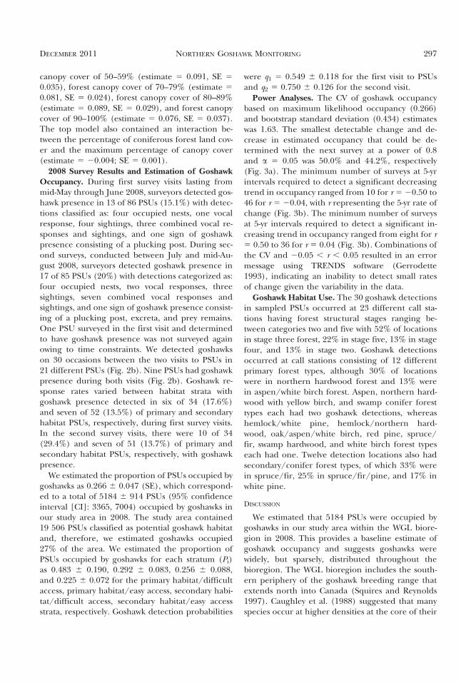
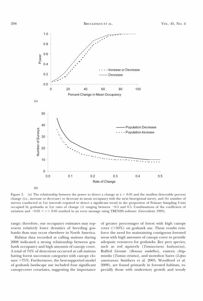
Power Analyses. The CV of goshawk occupancybased on maximum likelihood occupancy (0.266)and bootstrap standard deviation (0.434) estimateswas 1.63. The smallest detectable change and de-crease in estimated occupancy that could be de-termined with the next survey at a power of 0.8and a 5 0.05 was 50.0% and 44.2%, respectively(Fig. 3a). The minimum number of surveys at 5-yrintervals required to detect a significant decreasingtrend in occupancy ranged from 10 for r 5 20.50 to46 for r 5 20.04, with r representing the 5-yr rate ofchange (Fig. 3b). The minimum number of surveysat 5-yr intervals required to detect a significant in-creasing trend in occupancy ranged from eight for r5 0.50 to 36 for r 5 0.04 (Fig. 3b). Combinations ofthe CV and 20.05 , r , 0.05 resulted in an errormessage using TRENDS software (Gerrodette1993), indicating an inability to detect small ratesof change given the variability in the data.

Goshawk Habitat Use. The 30 goshawk detectionsin sampled PSUs occurred at 23 different call sta-tions having forest structural stages ranging be-tween categories two and five with 52% of locationsin stage three forest, 22% in stage five, 13% in stagefour, and 13% in stage two. Goshawk detectionsoccurred at call stations consisting of 12 differentprimary forest types, although 30% of locationswere in northern hardwood forest and 13% werein aspen/white birch forest. Aspen, northern hard-wood with yellow birch, and swamp conifer foresttypes each had two goshawk detections, whereashemlock/white pine, hemlock/northern hard-wood, oak/aspen/white birch, red pine, spruce/fir, swamp hardwood, and white birch forest typeseach had one. Twelve detection locations also hadsecondary/conifer forest types, of which 33% werein spruce/fir, 25% in spruce/fir/pine, and 17% inwhite pine.

DISCUSSION

We estimated that 5184 PSUs were occupied bygoshawks in our study area within the WGL biore-gion in 2008. This provides a baseline estimate ofgoshawk occupancy and suggests goshawks werewidely, but sparsely, distributed throughout thebioregion. The WGL bioregion includes the south-ern periphery of the goshawk breeding range thatextends north into Canada (Squires and Reynolds1997). Caughley et al. (1988) suggested that manyspecies occur at higher densities at the core of their

DECEMBER 2011 NORTHERN GOSHAWK MONITORING 297

range; therefore, our occupancy estimates may rep-resent relatively lower densities of breeding gos-hawks than may occur elsewhere in North America.

Habitat data recorded at calling stations during2008 indicated a strong relationship between gos-hawk occupancy and high amounts of canopy cover.A total of 74% of detections occurred at call stationshaving forest succession categories with canopy clo-sure .75%. Furthermore, the best-supported modelof goshawk landscape use included four significantcanopy-cover covariates, suggesting the importance

of greater percentages of forest with high canopycover (.50%) on goshawk use. These results rein-force the need for maintaining contiguous forestedareas with high amounts of canopy cover to provideadequate resources for goshawks. Key prey species,such as red squirrels (Tamiasciurus hudsonicus),Ruffed Grouse (Bonasa umbellus), eastern chip-munks (Tamias striatus), and snowshoe hares (Lepusamericanus: Smithers et al. 2005, Woodford et al.2008), are found primarily in forested habitats, es-pecially those with understory growth and woody

Figure 3. (a) The relationship between the power to detect a change at a 5 0.05 and the smallest detectable percentchange (i.e., increase or decrease) or decrease in mean occupancy with the next bioregional survey, and (b) number ofsurveys conducted at 5-yr intervals required to detect a significant trend in the proportion of Primary Sampling Unitsoccupied by goshawks at 5-yr rates of change (r) ranging between 20.5 and 0.5. Combinations of the coefficient ofvariation and 20.05 , r , 0.05 resulted in an error message using TRENDS software (Gerrodette 1993).

298 BRUGGEMAN ET AL. VOL. 45, NO. 4

debris (Litvaitis et al. 1985, Bayne and Hobson2000). Wiens et al. (2006a) documented the impor-tance of prey availability on survival of juvenile gos-hawks in northern Arizona and suggested forests bemanaged to support abundant prey populationswhile simultaneously providing forest structure suit-able for goshawk foraging (Beier and Drennan1997). Previous studies of goshawk nesting and for-aging habitats in the WGL bioregion also have indi-cated the importance of mature forest stands withhigh amounts of canopy cover (Rosenfield et al.1998, Boal et al. 2005).

Our 2008 surveys documented use of a variety offorest types by goshawks with most detections at callstations surrounded by northern hardwood and as-pen/white birch forests. Goshawk detection loca-tions in coniferous habitat types were primarily inspruce, fir, and pine forests. Additionally, the topmodel of goshawk landscape use included signifi-cant forest-type covariates with the percentages ofdeciduous, coniferous, and mixed deciduous/conif-erous forest all having coefficients with 95% confi-dence intervals not spanning zero. The use of avariety of forest types by goshawks in our studyagrees with previous work in the WGL bioregionand western North America (Boal et al. 2006). InMinnesota, foraging male goshawks used both ma-ture and old upland deciduous and coniferous for-est stands more frequently than expected based onavailability (Boal et al. 2005). Goshawk nests in Wis-consin have been found in a wide variety of treespecies with most occurring in northern hardwoodforest types (Woodford et al. 2008). Also, goshawksselected hardwood and mixed hardwood/coniferforests more than other cover types in Michigan(Lapinski 2000). Our results, along with the existingliterature on goshawk habitat use, suggest tree spe-cies has little influence on use of forests by goshawksand that canopy cover is a more influential factor.However, our results cannot be used to determinewhether goshawks selected for certain types becausewe did not have complete data on availability offorest types.

Our estimates of detection probabilities were low-er for the first survey visit (0.549; 95% CI: 0.292,0.807) than for the second (0.750; 95% CI: 0.485,1.000), but confidence intervals overlapped. Survey-ors detected goshawk presence in 17.6% of PSUsduring the first survey visit and 29.4% of PSUs forthe second survey visit in primary habitat strata. Fac-tors that may contribute to lower detectability ofgoshawks during the nestling period, specifically

during May, include variability in spring weatherthat may affect the timing of nesting and incuba-tion, and differences among individual goshawkswith respect to parental care (Dewey and Kennedy2001). Roberson et al. (2005) documented detec-tion probabilities of only 28% during the nestlingphase compared to 68% in the fledgling phase forgoshawk surveys in Minnesota. Nesting raptors ingeneral are often easier to locate later in the nestingseason because of adult defenses of the young andnest, and vocalizations from young (Steenhof andNewton 2007).

The proportion of PSUs with goshawk occupancyin primary habitat PSUs with difficult and easy ac-cess was 0.483 (95% CI: 0.033, 0.933) and 0.292(95% CI: 0.121, 0.463), respectively, and this differ-ence may be the result of multiple factors. First, thesample size for primary habitat/difficult access wasonly seven PSUs compared to 27 for the primaryhabitat/easy access stratum because the number ofPSUs in the sampling universe was lower for theprimary habitat/difficult access stratum. Resultsfrom the small sample may not represent the truepopulation, and the difference between probabili-ties may be a statistical artifact. Second, in contrastto private lands having access classified as difficult,public lands with easy access in the study area, suchas national and state forests and state parks, arelikely to be managed for multiple uses, includingrecreation and resource management that may de-crease the probability of goshawk use. Third, areasfarther from roads are less likely to receive humanuse, and if goshawks have low tolerance for humanactivity near nests or in breeding areas, more re-mote areas may exhibit a higher likelihood of gos-hawk use. We were unable to assess what factorsinfluenced differences in goshawk occupancy be-tween PSUs with difficult and easy access, but thiswarrants further examination in conjunction withfuture monitoring efforts. Occupancy modelinghas advanced since the Hargis and Woodbridge(2006) protocol and it may be worthwhile to esti-mate detection probabilities for each of the fourstrata to provide additional insights.

Our results illustrated the value of a well-definedsampling design for conducting surveys. Of 21 gos-hawk detections from different PSUs, 11 were in asecondary habitat strata with at least several of thesedetections in what would have been considered tobe low-quality habitat prior to our 2008 surveys. Incontrast, the 366 goshawk nest locations used todevelop the model of landscape use were obtained

DECEMBER 2011 NORTHERN GOSHAWK MONITORING 299

by assorted methods, including sightings near roadsor searching perceived high-quality habitat. Previ-ous work by Daw et al. (1998) found no differencesin forest structural properties between nest sitesfound opportunistically compared to those foundduring systematic surveys. However, they cautionedthat reliable density estimates, repeatability of meth-ods, and comparisons among years and studiescould only be attained through systematic methods(Daw et al. 1998). Whether potential bias existed inthe historical locations used to develop our predic-tive model is difficult to determine.

Power analyses indicated that a 50% change ingoshawk occupancy could be detected at a powerof 0.8 with a second bioregional survey. The esti-mate of occupancy for 2008 was 0.266 6 0.047and, therefore, an increase or decrease as small as0.133 may be determined at a power of 0.8. Poweranalyses indicated at least 10 surveys for a 5-yr rate ofchange of 20.5 must be conducted if surveys aredone every five years to detect a significant decreas-ing trend in the proportion of PSUs occupied bygoshawks. At least eight surveys for a 5-yr rate ofchange of 0.5 must be conducted to detect a signif-icant increasing trend in occupancy with time. Ofcourse, trade-offs exist between conducting surveysannually compared to every five years. Annual sur-veys are resource-intensive and require continuousfunding and partnership commitments, but they al-so provide the means of detecting smaller changesin occupancy over comparable timeframes becauseof the increased sample size of surveys. Annual sur-veys also provide a better opportunity to examineeffects of interannual climate variability on goshawkpopulation trends and to understand how muchvariation in occupancy occurs among years. Surveysconducted every five years are less resource-inten-sive and allow project collaborators to commit fundsto other priority projects during years without sur-veys.

Our results provide the first estimate of goshawkoccupancy for our study area in the WGL bioregionbased on the Hargis and Woodbridge (2006) mon-itoring protocol. Given its potential for providinginsights into both management and ecological is-sues, the monitoring is likely to be implementedin other bioregions throughout the country overthe next several years. However, based on our find-ings and the amount of resources committed to theproject, we recommend the surveys best be used todetermine one-time population status and offer in-sights into locations of goshawks for future intensive

research by federal and state agencies as opposed todetermining population trend with multiple surveysover time. Based on surveying 86 PSUs in the WGLbioregion, our power analyses indicated that only a50% change in the occupancy of PSUs could bedetected with the next bioregional survey. Projectpartners provided .$200 000 plus additional in-kind effort to complete the 2008 surveys; attemptingto determine a trend with that kind of commitmentevery five years is not likely to be worthwhile nomatter the economic climate.

We offer the following additional suggestions forinstituting bioregional surveys and monitoringbased on our experience and findings. First, surveysshould encompass all land ownership types and notjust U.S. Forest Service lands or other public lands.Inference about a regional population can only beobtained using a sampling design that includes sur-veying both public and private lands if they includepotential goshawk habitat. Although this approachrequires cooperation among project collaboratorsand private landowners, it offers valuable insightsinto goshawk-habitat associations not possible withmonitoring only public lands. Second, we recom-mend using a stratified sampling design, as opposedto random sampling of PSUs, to increase the preci-sion of the occupancy estimate while operating witha fixed budget to ensure surveying both primaryand secondary habitats (Woodbridge and Hargis2006). Development of a stratified sampling designrequires some knowledge of goshawk landscape use,which can be obtained using a combination of ex-isting location data and GIS layers spanning theentire bioregion. GIS layers of habitat attributesfor national and state forests may provide detailand high resolution, but these layers may not beavailable across the entire bioregion. We were con-strained to use land and forest canopy cover datawith 30-m resolution that provided coverage acrossall types of land ownership because the WGL bio-region consists of a combination of public and pri-vate lands. Although some misclassification of pri-mary and secondary habitat PSUs undoubtedlyoccurred, use of a random sampling design withno knowledge of prior goshawk landscape usewould have been less efficient and resulted in anoccupancy estimate with higher variance.

ACKNOWLEDGMENTS

This project was completed with funding and supportfrom the U.S. Forest Service, U.S. Geological Survey’s Min-nesota Cooperative Fish and Wildlife Research Unit, Uni-versity of Minnesota, Chequamegon-Nicolet National For-

300 BRUGGEMAN ET AL. VOL. 45, NO. 4

est, Chippewa National Forest, Hiawatha National Forest,Ottawa National Forest, Superior National Forest, Minne-sota Department of Natural Resources, Wisconsin Depart-ment of Natural Resources, Michigan Natural Features In-ventory, Plum Creek Timber Company, and PotlachCorporation. We would like to acknowledge the numeroussurveyors who participated in data collection efforts andthe private landowners who provided access to their landduring surveys. We would also like to acknowledge J. Bald-win, D. Johnson, C. Voijta, and one anonymous reviewerwho provided suggestions and comments that improvedprevious drafts of this manuscript. Use of trade names doesnot imply endorsement by either the U.S. Geological Sur-vey or the University of Minnesota.

LITERATURE CITED

ALLISON, P.D. 1999. Logistic regression using the SAS sys-tem: theory and application. SAS Institute, Inc., Cary,NC U.S.A.

ANDERSEN, D.E., S. DESTEFANO, M.I. GOLDSTEIN, K. TITUS, C.CROCKER-BEDFORD, J.J. KEANE, R.G. ANTHONY, AND R.N.ROSENFIELD. 2005. Technical review of the status ofNorthern Goshawks in the western United States. Jour-nal of Raptor Research 39:192–209.

BAILEY, R.G. 1995. Description of the ecoregions of theUnited States. Miscellaneous Publication No. 1391, Sec-ond Ed. revised. USDA, Washington, DC U.S.A.

BAYNE, E. AND K. HOBSON. 2000. Relative use of contiguousand fragmented forest by red squirrels (Tamiasciurushudsonicus). Canadian Journal of Zoology 78:359–365.

BEIER, P. AND J.E. DRENNAN. 1997. Forest structure and preyabundance in foraging areas of Northern Goshawks.Ecological Applications 7:564–571.

BOAL, C.W., D.E. ANDERSEN, AND P.L. KENNEDY. 2005. For-aging and nesting habitat of breeding male NorthernGoshawks in the Laurentian Mixed Forest Province,Minnesota. Journal of Wildlife Management 69:1516–1527.

———, ———, ———, AND A.M. ROBERSON. 2006. North-ern Goshawk ecology in the western Great Lakes re-gion. Studies in Avian Biology 31:126–134.

BRUGGEMAN, J.E., D.E. ANDERSEN, AND J.E. WOODFORD.2009. Bioregional monitoring for Northern Goshawksin the western Great Lakes. Final Report. http://wiatri.net/inventory/Raptors/goshawks/reports.htm (last ac-cessed 1 February 2011).

BURNHAM, K.P. AND D.R. ANDERSON. 2002. Model selectionand multimodel inference: a practical information-theoretic approach, Second Ed. Springer-Verlag, NewYork, NY U.S.A.

CAUGHLEY, G., D. GRICE, R. BARKER, AND B. BROWN. 1988.The edge of the range. Journal of Animal Ecology57:771–785.

COHEN, J. 1992. A power primer. Psychology Bulletin112:155–159.

DAW, S.K., S. DESTEFANO, AND R.J. STEIDL. 1998. Does surveymethod bias the description of Northern Goshawknest-site structure? Journal of Wildlife Management62:1379–1384.

DEWEY, S.R. AND P.L. KENNEDY. 2001. Effects of supplemen-tal food on parental-care strategies and juvenile survivalof Northern Goshawks. Auk 118:352–365.

DOYLE, F.I. AND J.M.N. SMITH. 2001. Raptors and scaven-gers. Pages 378–404 in C.J. Krebs, S. Boutin, and R.Boonstra [EDS.], Ecosystem dynamics of the boreal for-est. Oxford University Press, New York, NY U.S.A.

EFRON, B. AND R.J. TIBSHIRANI. 1993. An introduction to thebootstrap. Chapman and Hall, New York, NY U.S.A.

FAIRHURST, G.D. AND M.J. BECHARD. 2005. Relationshipsbetween winter and spring weather and Northern Gos-hawk (Accipiter gentilis) reproduction in northern Ne-vada. Journal of Raptor Research 39:229–236.

GERRODETTE, T. 1987. A power analysis for detectingtrends. Ecology 68:1364–1372.

———. 1993. TRENDS: software for a power analysis oflinear regression. Wildlife Society Bulletin 21:515–516.

HARGIS, C.D. AND B. WOODBRIDGE. 2006. A design for mon-itoring Northern Goshawks (Accipiter gentilis) at thebioregional scale. Studies in Avian Biology 31:274–287.

HOMER, C., C. HUANG, L. YANG, B. WYLIE, AND M. COAN.2004. Development of a 2001 National Land Cover Da-tabase for the United States. Photogrammetric Engineeringand Remote Sensing 70:829–840.

HOSMER, D.W. AND S. LEMESHOW. 2000. Applied logistic re-gression. John Wiley and Sons, Inc., New York, NY U.S.A.

HUANG, C., C. HOMER, AND L. YANG. 2003. Regional forest landcover characterization using Landsat type data. Pages389–410 in M. Wulder and S. Franklin [EDS.], Remotesensing of forest environments: concepts and case studies.Kluwer Academic Publishers, Norwell, MA U.S.A.

———, L. YANG, B. WYLIE, AND C. HOMER. 2001. A strategy forestimating tree canopy density using Landsat 7 ETM+ andhigh resolution images over large areas. Proceedings ofthe Third International Conference on Geospatial Infor-mation in Agriculture and Forestry, Denver, CO U.S.A.

KENNEDY, P.L. AND D.W. STAHLECKER. 1993. Responsivenessof nesting Northern Goshawks to taped broadcasts of 3conspecific calls. Journal of Wildlife Management 57:249–257.

LAPINSKI, N.W. 2000. Habitat use and productivity of theNorthern Goshawk in the Upper Peninsula of Michi-gan. M.S. thesis, Northern Michigan Univ., Marquette,MI U.S.A.

LITVAITIS, J.A., J.A. SHERBURNE, AND J.A. BISSONETTE. 1985.Influence of understory characteristics on snowshoehare habitat use and density. Journal of Wildlife Manage-ment 49:866–873.

MANLY, B.F., L.L. MCDONALD, D.L. THOMAS, T.L. MCDON-

ALD, AND W.P. ERICKSON. 2002. Resource selection byanimals: statistical design and analysis for field studies.Chapman and Hall, New York, NY U.S.A.

MCNAB, W.H., D.T. CLELAND, J.A. FREEOUF, J.E. KEYS, JR.,G.J. NOWACKI, AND C.A. CARPENTER [COMPILERS]. 2007.Description of ecological subregions: sections of theconterminous United States. U.S. Forest Service Gen.Tech. Rep. WO-76B, Washington, DC U.S.A.

DECEMBER 2011 NORTHERN GOSHAWK MONITORING 301

POLLOCK, K.H., J.D. NICHOLS, T.R. SIMONS, G.L. FARNS-

WORTH, L.L. BAILEY, AND J.R. SAUER. 2002. Large scalewildlife monitoring studies: statistical methods for de-sign and analysis. Environmetrics 13:105–119.

R DEVELOPMENT CORE TEAM. 2008. R: a language and envi-ronment for statistical computing. R Foundation forStatistical Computing, Vienna, Austria. http://www.R-project.org (last accessed 18 July 2010).

REYNOLDS, R.T., R.T. GRAHAM, AND D.A. BOYCE, JR. 2008.Northern Goshawk habitat: an intersection of science,management, and conservation. Journal of Wildlife Man-agement 72:1047–1055.

———, J.D. WIENS, S.M. JOY, AND S.R. SALAFSKY. 2005. Sam-pling considerations for demographic and habitat stud-ies of Northern Goshawks. Journal of Raptor Research39:274–285.

ROBERSON, A.M., D.E. ANDERSEN, AND P.L. KENNEDY. 2005.Do breeding phase and detection distance influencethe effective area surveyed for Northern Goshawks?Journal of Wildlife Management 69:1240–1250.

ROSENFIELD, R.N., T.C.L. DOOLITTLE, D.R. TREXEL, AND J.BIELEFELDT. 1998. Breeding distribution and nest-sitehabitat of Northern Goshawks in Wisconsin. Journal ofRaptor Research 32:189–194.

SALAFSKY, S.R., R.T. REYNOLDS, AND B.R. NOON. 2005. Pat-terns of temporal variation in goshawk reproductionand prey resources. Journal of Raptor Research 39:237–246.

SANDER, H., S. POLASKY, AND R.G. HAIGHT. 2010. The valueof urban tree cover: a hedonic property price model inRamsey and Dakota counties, Minnesota, USA. Ecologi-cal Economics 69:1646–1656.

SIDERS, M.S. AND P.L. KENNEDY. 1994. Nesting habitat ofaccipiter hawks: is body size a consistent predictor ofnest habitat characteristics? Studies in Avian Biology16:92–96.

SMITHERS, B.L., C.W. BOAL, AND D.E. ANDERSEN. 2005.Northern Goshawk diet in Minnesota: an analysis usingvideo recording systems. Journal of Raptor Research39:264–273.

SQUIRES, J.R. AND P.L. KENNEDY. 2006. Northern Goshawkecology: an assessment of current knowledge and infor-mation needs for conservation and management. Stud-ies in Avian Biology 31:8–62.

——— AND R.T. REYNOLDS. 1997. Northern Goshawk (Ac-cipiter gentilis). In A. Poole and F. Gill [EDS.], The birdsof North America, No. 298. The Academy of NaturalSciences, Philadelphia, PA U.S.A. and The AmericanOrnithologists’ Union, Washington, DC U.S.A.

——— AND L.F. RUGGIERO. 1996. Nest-site preference ofNorthern Goshawks in southcentral Wyoming. Journalof Wildlife Management 60:170–177.

STEENHOF, K. AND I. NEWTON. 2007. Assessing nesting suc-cess and productivity. Pages 181–192 in D.M. Bird andK.L. Bildstein [EDS.], Raptor research and manage-ment techniques, Hancock House Publishers, Blaine,WA U.S.A.

THOMPSON, S.K. 2002. Sampling. John Wiley and Sons, Inc.,New York, NY U.S.A.

WALTON, J.T., D.J. NOWACK, AND E.J. GREENFIELD. 2008. As-sessing urban forest canopy cover using airborne orsatellite imagery. Arboriculture and Urban Forestry34:334–340.

WIENS, J.D., B.R. NOON, AND R.T. REYNOLDS. 2006a. Post-fledgling survival of Northern Goshawks: the impor-tance of prey abundance, weather, and dispersal. Eco-logical Applications 16:406–418.

———, R.T. REYNOLDS, AND B.R. NOON. 2006b. Juvenilemovement and natal dispersal of Northern Goshawksin Arizona. Condor 108:253–269.

WOODBRIDGE, B. AND C.D. HARGIS. 2006. Northern Gos-hawk inventory and monitoring technical guide. U.S.Forest Service Gen. Tech. Rep. WO-71, Washington,DC U.S.A.

WOODFORD, J.E., C.A. ELORANTA, AND K.D. CRAIG. 2008.Nest monitoring and prey of Northern Goshawks inWisconsin. Passenger Pigeon 70:171–179.

Received 26 May 2010; accepted 11 July 2011Associate Editor: Karen Steenhof

APPENDIX

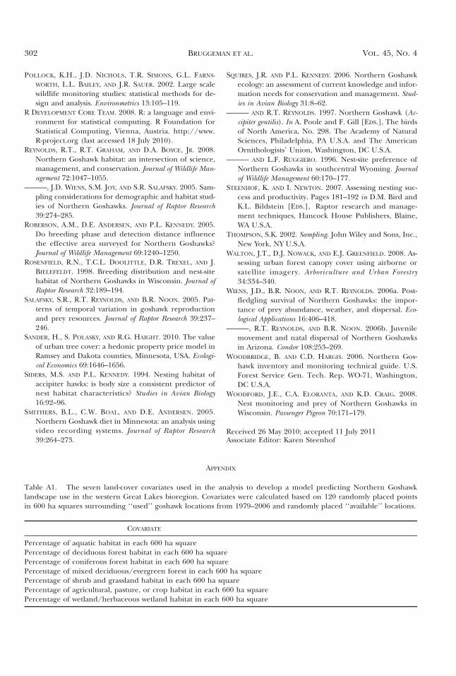
Table A1. The seven land-cover covariates used in the analysis to develop a model predicting Northern Goshawklandscape use in the western Great Lakes bioregion. Covariates were calculated based on 120 randomly placed pointsin 600 ha squares surrounding ‘‘used’’ goshawk locations from 1979–2006 and randomly placed ‘‘available’’ locations.

COVARIATE

Percentage of aquatic habitat in each 600 ha squarePercentage of deciduous forest habitat in each 600 ha squarePercentage of coniferous forest habitat in each 600 ha squarePercentage of mixed deciduous/evergreen forest in each 600 ha squarePercentage of shrub and grassland habitat in each 600 ha squarePercentage of agricultural, pasture, or crop habitat in each 600 ha squarePercentage of wetland/herbaceous wetland habitat in each 600 ha square

302 BRUGGEMAN ET AL. VOL. 45, NO. 4

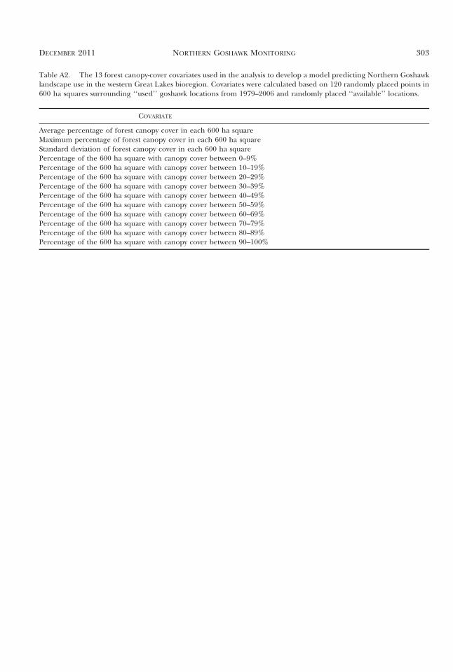
Table A2. The 13 forest canopy-cover covariates used in the analysis to develop a model predicting Northern Goshawklandscape use in the western Great Lakes bioregion. Covariates were calculated based on 120 randomly placed points in600 ha squares surrounding ‘‘used’’ goshawk locations from 1979–2006 and randomly placed ‘‘available’’ locations.

COVARIATE

Average percentage of forest canopy cover in each 600 ha squareMaximum percentage of forest canopy cover in each 600 ha squareStandard deviation of forest canopy cover in each 600 ha squarePercentage of the 600 ha square with canopy cover between 0–9%Percentage of the 600 ha square with canopy cover between 10–19%Percentage of the 600 ha square with canopy cover between 20–29%Percentage of the 600 ha square with canopy cover between 30–39%Percentage of the 600 ha square with canopy cover between 40–49%Percentage of the 600 ha square with canopy cover between 50–59%Percentage of the 600 ha square with canopy cover between 60–69%Percentage of the 600 ha square with canopy cover between 70–79%Percentage of the 600 ha square with canopy cover between 80–89%Percentage of the 600 ha square with canopy cover between 90–100%

DECEMBER 2011 NORTHERN GOSHAWK MONITORING 303