Biomechanics of Acute Total Hip Arthroplasty after

Acetabular Fracture: Plate vs Cable Fixation

by

Mina S. R. Aziz

A thesis submitted in conformity with the requirements

for the degree of Master of Science

Institute of Medical Science

University of Toronto

© Copyright by Mina S. R. Aziz 2014

ii

Biomechanics of Acute Total Hip Arthroplasty after

Acetabular Fracture: Plate vs Cable Fixation

Mina S. R. Aziz

Master of Science

Institute of Medical Science

University of Toronto

2014

Abstract

The incidence of complex acetabular fractures is increasing worldwide, especially in the elderly.

Fixation methods currently used surgically have no biomechanical justification. Therefore, this

study compared the standard plate versus three cable techniques for anterior column plus

posterior hemitransverse acetabular fractures in synthetic hemipelves. Phase I employed FEA

validated by non-destructive mechanical testing. Phase II entailed destructive comparison of the

superior cabling method from Phase I versus the standard plating procedure. Phase I identified

the Mouhsine cable method as providing the best mechanical stability (i.e. based on lowest peak

bone stress) among the cable techniques. Phase II demonstrated the Plate group’s superiority

over the Mouhsine group for 2 outcomes (i.e. stiffness and failure force at clinical failure), its

inferiority for 2 outcomes (i.e. failure displacement and gapping for posterior markers at

mechanical failure), and statistical equivalence for the remaining outcomes. This investigation

has implications for surgical repair of this injury.

iii

Acknowledgements

I am extremely grateful to my supervisor, Dr. Emil Schemitsch, for giving me this opportunity of

pursuing a Master’s program at the University of Toronto, Institute of Medical Science under his

continuous guidance, mentorship and support. You were always there by my side to offer help,

whenever needed. You made me feel deeply rooted into the big team of clinicians and

researchers. Thank you very much for the great level of trust and responsibility you gave me, and

for your obvious generosity over the past and most amazing two years of my life. I believe I will

never find such a lovely, respectful and outstanding supervisor.

I regard forming excellent work and personal relationship with Dr. Radovan Zdero to be the

greatest life-time gain I have achieved from this research. I am very happy to get to know such a

wonderful, helpful and supportive character. Thank you very much for your tireless

encouragement throughout my Master’s program, and for the countless hours you spent teaching

me many technical and academic aspects of my research.

I owe much gratitude to all the exceptional members of my thesis committee, who provided

much insight, encouragement and guidance throughout my studies, namely Drs. Albert Yee and

Hans Kreder. I also thank Dr. Joanna Sale for officially supervising me at the Collaborative

Musculoskeletal Program. I would also like to thank Dr. Omar Dessouki and Saeid Samiezadeh

for their valuable assistance with my research project. I wish to acknowledge all the initiative

offered by every staff member at the Institute of Medical Science, and also the grant provided by

the Ontario Graduate Scholarship in Science and Technology – David E. Hastings at UofT,

which made a big difference in accomplishing my research.

Most importantly, I owe my greatest appreciation to my 3 brothers and sisters-in-law from oldest

to youngest: Mike and Janet, Beshoy and Maria, Ibram and Angie, and particularly my mom,

Nadia, who held my hand all the way through my hard times and difficulties. All of them were,

are and, I am sure, will continue to be a tireless source of love, comfort and encouragement.

Above all, words cannot express my deepest gratitude to my lovely and loving Lord and Savior

Jesus Christ, who is my ceaseless strength, victory, joy, and love. As the Bible says “I can do all

things through Christ, who strengthens me” Philippians 4:13.

iv

Contributions

Mina Aziz (author) was responsible for execution of the experiments, data analyses,

computational analyses, and preparation of this thesis. The latter included the preparation of each

section with all the integrated tables and figures, except for most of the figures in Chapter 2

(Literature Review), where every one of the figures is cited in its caption. The contributions

made by others are officially and comprehensively listed below:

Dr. Emil H. Schemitsch (Supervisor and Program Advisory Committee (PAC) Member):

Mentorship, laboratory resources, support, and guidance in planning and execution of this body

of work.

Dr. Radovan Zdero (Research Director of the Martin Orthopaedic Biomechanics Laboratory):

Laboratory facilities, guidance in planning, execution and analysis of the experimental and

computational parts of this study.

Dr. Omar Dessouki: Assistance in preparing all the specimens for the experimental portion of the

project.

Saeid Samiezadeh: Assistance in the preparation and analysis of the computational portion of the

project.

Dr. Albert Yee (PAC Member): Guidance with the planning, execution, and analysis of the

project.

Dr. Hans Kreder (PAC Member): Guidance with the planning, execution, and analysis of the

project.

Dr. Joanna Sale (Supervisor for the Collaborative Program in Musculoskeletal Sciences):

Mentorship and guidance with the various aspects of this specific program.

Dr. Habiba Bougherara: Assistance with some questions about the preparation and analysis of

the computational part of the study.

v

Table of Contents

ACKNOWLEDGEMENTS ……………………………………………………. iii

CONTRIBUTIONS ………………………………………………………..…… iv

TABLE OF CONTENTS ………………………………………………...…...… v

LIST OF TABLES ……………………………………………………………… ix

LIST OF FIGURES …………………………………………………………...… x

LIST OF ABBREVIATIONS ……………………………………………........ xvi

CHAPTER 1 INTRODUCTION ………………………………………….. 1

1.1 Overview ………………………………………………………………..… 1

1.2 Thesis Outline …….………………………………………………………. 2

CHAPTER 2 LITERATURE REVIEW (BACKGROUND) ……………. 4

2.1 Anatomy of the Hip ………………………………………………………. 4

2.1.1 Descriptive Anatomy of the Hip ……………………………………. 4

2.1.1.1 Hip Bone …………………………………………….… 4

2.1.1.2 Acetabulum ……………………………………………. 7

2.1.1.3 Hip Joint ………………………………………………. 8

2.1.1.4 Hip Muscles and Movements …………………………. 9

2.1.2 Surgical Anatomy of the Hip ……………………………………….. 9

2.2 Biomechanics of the Hip ………………………………………………... 12

2.2.1 Overview …………………………………………………………... 12

2.2.2 Force Applied to the Greater Trochanter ………………………..… 13

2.2.3 Force Applied to the Flexed Knee ………………………………… 14

2.3 Acetabular Fractures ………………………………………………...…. 16

2.3.1 Epidemiology ……………………………………………………… 16

vi

2.3.1.1 Incidence and Prevalence ……………………………. 16

2.3.1.2 Mechanism of Injury ……………………………….... 20

2.3.2 Classification ……………………………………………………… 21

2.3.2.1 History of Acetabular Fracture Classification ……….. 21

2.3.2.2 Current Acetabular Fracture Classification ………….. 22

2.4 Associated Anterior and Posterior Hemitransverse Fractures ………. 22

2.4.1 Nomenclature …..………………………………………………..… 22

2.4.2 Incidence ………………………………………………………...… 23

2.4.3 Morphology ………………………………………………………... 24

2.4.3.1 Anterior Component …………………………………. 24

2.4.3.2 Posterior Component ………………………………… 25

2.5 Management of Acetabular Fractures ………………………………… 26

2.5.1 Overview ………………………………………………………...… 26

2.5.2 Conservative Treatment …………………………………………… 29

2.5.2.1 Indications …………………………………………… 29

2.5.2.2 Methods ……………………………………………… 29

2.5.2.3 Complications ……………………………………...… 30

2.5.3 Surgical Treatment ………………………………………...………. 30

2.5.3.1 Surgical Access ………………………………...……. 30

2.5.3.2 Open Reduction and Internal Fixation (ORIF) ………. 31

2.5.3.3 Combined Hip Procedure (ORIF + Acute THA) ….… 32

2.6 Biomechanical Studies for Acetabular Fracture Fixation ……………. 33

CHAPTER 3 RESEARCH AIMS AND HYPOTHESES ………………. 36

3.1 Research Aims ………………………………………………………...… 36

3.2 Speculated Hypotheses ………………………………………………….. 37

CHAPTER 4 METHODS ……………………………………………….... 38

4.1 Overview ……………………………………………………………….... 38

4.2 Phase I – Non-Destructive Mechanical Analysis …………………….... 39

4.2.1 Experimental Methodology ………………………………………... 39

4.2.1.1 Hemipelvis Properties ……………………………..… 39

4.2.1.2 Specimen Preparation ………………………………... 40

vii

4.2.1.3 Mechanical Test Jig ………………………………….. 50

4.2.1.4 Strain Gauges ………………………………………… 52

4.2.1.5 Mechanical Tests …………………………………….. 56

4.2.2 Finite Element Analysis (FEA) ……………………………………. 58

4.2.2.1 CAD Models …………………………………………. 58

4.2.2.2 Component Assembly ……………………………..… 59

4.2.2.3 Assembly Processing ………………………………… 60

4.2.2.4 Boundary Conditions ……………………………….... 60

4.2.2.5 Material Properties ………………………………...… 64

4.2.2.6 Meshing ……………………………………………… 64

4.2.2.7 FE Analysis ………………………………………….. 65

4.3 Phase II – Destructive Mechanical Testing ……………………………. 66

4.3.1 Selection of the Two Best Repair Methods ……………………….. 66

4.3.2 Marker Placement …………………………………………………. 67

4.3.3 Mechanical Testing ………………………………………………... 68

4.3.4 Data Analysis …………………………………………………….... 69

4.3.5 Statistical Analysis ………………………………………………… 70

CHAPTER 5 RESULTS ………………………………………………….. 71

5.1 Phase I: Non-Destructive Analysis of Hemipelvises …………………... 71

5.1.1 Experimental Validation of FEA ………………………………….. 71

5.1.2 FEA Stress Maps at 3 x Body Weight ……………….................... 73

5.1.2.1 Bone Stress Maps ……………………………………. 73

5.1.2.2 Stress Maps for Acetabular Cups and Implants …...… 75

5.1.3 FEA Stiffnesses at 3 x Body Weight …………………………….... 76

5.2 Phase II: Destructive Analysis of Hemipelvises ……………………….. 77

5.2.1 Raw Data …………………………………………………………... 77

5.2.2 Stiffness ……………………………………………………………. 79

5.2.3 Failure Displacement …………………………………………….... 79

5.2.4 Failure Force ………………………………………………………. 80

5.2.5 Failure Energy ……………………………………………………... 81

5.2.6 Sliding …………………………………………………………...… 82

5.2.7 Gapping ………………………………………………………….… 83

5.2.8 Failure Modes ……………………………………………………... 84

viii

5.2.9 Power Analysis ……………………………………………………. 86

CHAPTER 6 DISCUSSION ……………………………………………… 87

6.1 General Findings ………………………………………………………... 87

6.2 Comparison to Prior Biomechanical Studies ………………………….. 87

6.3 Biomechanical Implications ……………………………………………. 92

6.4 Surgical Implications …...…………………………………………….… 96

6.5 Possible Limitations …………………………………………………….. 99

CHAPTER 7 CONCLUSIONS ………………………………………..... 103

CHAPTER 8 FUTURE DIRECTIONS ………………………………… 104

8.1 Biomechanical Optimization of Complex Acetabular Fracture Fixation

using Computational Modeling and Human Cadaveric Testing …… 104

8.1.1 Definition of the Research Question ……………………………... 104

8.1.2 Importance of the Research Question ……………………………. 106

8.1.3 Research Design ………………………………………………….. 107

8.1.3.1 General Strategy …………………………………..... 107

8.1.3.2 Phase 1 – Computational Modeling ………………... 107

8.1.3.3 Phase 2 – Human Cadaveric Testing ……………….. 108

REFERENCES ……………………………………………………………..… 110

ix

List of Tables

Table 2.1 Pelvic fracture characteristics, obtained from Royal Infirmary of Edinburgh,

Scotland in years 2000 vs 2007/8 …………………………..………………… 17

Table 2.2 Pelvic vs acetabular fracture characteristics, Royal Infirmary of Edinburgh,

Scotland in years 2000 vs 2007/8 …………………………………………..… 18

Table 2.3 Pelvic vs acetabular fractures, obtained from the R. Adams Cowley Shock

Trauma Center in Baltimore, Maryland, USA in 2007 …………………..… 19

Table 4.1 Mechanical properties of the materials assigned in the six FE models ….… 64

Table 4.2 Number of nodes and elements for each mesh of the six FE models .……… 65

Table 5.1 Experimental Von Mises Stress Values in MPa. SG = strain gauge ………. 71

Table 5.2 FEA Von Mises Stress Values in MPa at each Strain Gauge Location. SG =

strain gage ……………………………………………………………………... 71

Table 5.3 FEA Displacement, Stiffness, and Percentage Increase in Stiffness in Respect

to the Intact Group at a Force of 2207N i.e. 3 x body weight ……………… 76

Table 5.4 Averages of the One- and Two-tailed Post-Hoc Power Analysis for all Phase

II Outcomes ………………………………………………………………….... 86

Table 6.1 A general comparison of the outcomes of some biomechanical studies

performed on acetabular fractures presenting the conventional methods

used……………………………………………………………………………... 90

Table 8.1 Surgical repair methods to be biomechanically tested [4,16,17]. AC =

anterior column, AIIS = anterior inferior iliac spine, IC = iliac crest, IIF =

internal iliac fossa, PC = posterior column, PW = posterior wall ………... 108

x

List of Figures

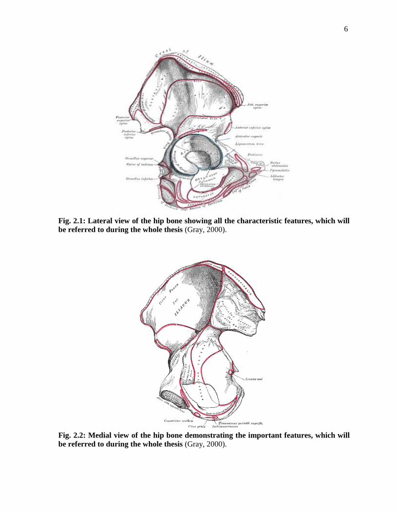
Fig. 2.1 Lateral view of the hip bone showing all the characteristic features, which

will be referred to during the whole thesis …………………………………… 6

Fig. 2.2 Medial view of the hip bone demonstrating the important features, which will

be referred to during the whole thesis ………………………………………… 6

Fig. 2.3 Anterior view of the pelvis in the anatomical orientation, where the

acetabulum is facing anteriorly, laterally, and downwards …………………. 8

Fig. 2.4 Surgical anatomy of the hip bone. Red: Posterior column, White: Anterior

column, Blue: Ischio-pubic ramus. A. Lateral view, B. Obturator-Oblique

view, C. Iliac-Oblique view …………………………………………………... 11

Fig. 2.5 Free body diagram of force (F) acting on the greater trochanter at point (A)

transmitting a net force (F’) through the centre of the femoral head (C),

yielding an impact on the acetabulum at point (I), with an ellipse of influence

(shaded area) ………………………………………………………………..… 13

Fig. 2.6 A. Transverse section through the hip joint showing the effect of different

degrees of internal/external rotation of the femur on locations of force

transmission. B. Coronal section of the hip joint at 20° of internal rotation

illustrating the effect of different abduction/adduction on the lines of force

transmission ………………………………………………………………….... 14

Fig. 2.7 Transverse section through the hip joint, hip is flexed at 90°, showing the

effect of wide range of abduction/adduction on sites of force transmission.

Force is applied through the knee ………………………………………….... 15

Fig. 2.8 Distribution curves for pelvic fractures (type E) vs acetabular fractures (type

G) at the Royal Infirmary of Edinburgh, Scotland ………………………… 18

xi

Fig. 2.9 The distribution curve for both pelvic and acetabular fractures (type C) from

the R. Adams Cowley Shock Trauma Center in Baltimore, Maryland, USA in

2007 …………………………………………………………………………..… 20

Fig. 2.10 Schemes of associated anterior with posterior hemitransverse acetabular

fracture. A. High anterior column acetabular fracture with posterior

hemitransverse, lateral view, B. medial view, C. Middle anterior column

fracture with posterior hemitransverse, lateral view, D. Medial view, E.

Anterior wall fracture with posterior hemitransverse, lateral view, F. Medial

view …………………………………………………………………………….. 25

Fig. 2.11 Algorithm for the management of acetabular fractures in the elderly,

developed by the specialized team of Helfet and co-workers ………………. 28

Fig. 4.1 Synthetic hemipelvis (Model #3405-1, Sawbones, Vashon, WA, USA)

demonstrating its dimensions; a) 235mm, b) Diameter of the acetabulum=

55mm, c) 140mm, and d) 175mm ……………………………………………. 40

Fig. 4.2 Reaming of the acetabulum, creating the AHT fracture, and reducing it … 43

Fig. 4.3 Left: acetabular shell insertion. Right: acetabular liner insertion ………… 44

Fig. 4.4 The “Plate” fixation method. A posterior column plate with an anterior

column lag screw. Left: lateral view. Right: medial view. An acetabular cup

was inserted …………………………………………………………………… 48

Fig. 4.5 The “Mears” fixation method. A 2.0 mm braided cable with clamp was

employed. Left: lateral view. Right: medial view. An acetabular cup was

inserted ………………………………………………………………………… 48

Fig. 4.6 The “Kang” fixation method. Two 2.0 mm braided cables were utilized. Left:

lateral view. Right: medial view. An acetabular cup was inserted ………… 49

xii

Fig. 4.7 The “Mouhsine” fixation method. One 2.0 mm braided cable was used. Left:

lateral view. Right: medial view. An acetabular cup was installed ………... 49

Fig. 4.8 Mechanical test setup consisting of 2 metal cubes bolted to each other, a side

plate, and a spacer on the side. The front face of the upper cube was used for

mounting the SI region and the top surface of the side block was used for

mounting the SP region ………………………………………………………. 51

Fig. 4.9 The setup with an intact with cup specimen mounted on it. Left: Lateral view

of the setup showing the SP mounting screw. Right: Anterior view of the

setup showing the three SI mounting screws ………………………………... 51

Fig. 4.10 A) A DSub showing its internal electric circuit and connections, B) The eight-

channel amplifier of the Cronos-PL system, C) A rectangular rosette strain

gauge demonstrating its three grids numbered 1, 2, and 3 by the

manufacturer ………………………………………………………………….. 54

Fig. 4.11 A) Lateral view of the hemipelvis showing SG1 and 2, B) Meidal view of the

hemipelvis illustrating SG3, 4, and 5, C) The Cronos connected to the DSubs,

which in turn are connected to alligator clips. These clips were connected to

the wires coming out of the SG. SG= Strain Gauge ………………………… 55

Fig. 4.12 A Plate specimen mounted on the Instron. Left: Anterior view, right: lateral

view …………………………………………………………………………….. 57

Fig. 4.13 A 3D CAD Model of the hemipelvis. Left: lateral view, right: medial view . 62

Fig. 4.14 Assembly of component parts in the same orientation as experiments. Left:

Intact group, right: Cup group ………………………………………………. 62

Fig. 4.15 Assembly of component parts oriented exactly as experiments. Left: Plate

group, right: Mears group …………………………………………………… 63

xiii

Fig. 4.16 Assembly of component parts mounted on the setup and oriented as in

experiments. Left: Kang group, right: Mouhsine group …………………... 63

Fig. 4.17 Meshing of the FE models. A Plate model was presented here as an example.

Left: showing the whole mesh, right: a magnified view of the acetabular cup,

acetabulum, plate and screws, as well as setup device ……………………… 66

Fig. 4.18 Three pictures extracted from video records of the Plate group showing the

position of the markers along the posterior hemitransverse fracture at the

starting position without any displacement (left), at clinical failure point

(middle), and at mechanical failure point (right) …………………………… 68

Fig. 4.19 Three pictures of the Mouhsine group extracted from video records,

illustrating the position of the markers along the transverse fracture at the

starting position without any displacement (left), at clinical failure point

(middle), and at mechanical failure point (right) …………………………… 68

Fig. 5.1 FEA Von Mises Stress Validation Graph. All data points, except one, from

all six experimental and FEA groups were plotted together since strain gauge

positions were exactly the same. Ideal correlation would result in Slope=1

and R=1 ………………………………………………………………………... 72

Fig. 5.2 FEA Peak Bone Von Mises Stress in MPa for all Six FE Groups …………. 73

Fig. 5.3 FEA Von Mises Stress Maps at three times body weight of an average 75Kg

person i.e. Force= 2207N. Peak bone stress values and locations are

demonstrated in the pictures. Left = Intact Model, Right = Cup Model ….. 74

Fig. 5.4 FEA Von Mises Stress Maps at three times body weight of an average 75Kg

person i.e. Force= 2207N. Peak bone stress values and locations are

demonstrated in the pictures. Left = Plate Model, Right = Mears Model … 74

xiv

Fig. 5.5 FEA Von Mises Stress Maps at three times body weight of an average 75Kg

person i.e. Force= 2207N. Peak bone stress values and locations are

demonstrated in the pictures. Left = Kang Model, Right = Mouhsine

Model…………………………………………………………………………… 75

Fig. 5.6 FEA Stiffness for all Six Models at a Load of 3 Times Body Weight ……… 77

Fig. 5.7 A raw data graph for one specimen representative of the Plate group

showing the points of MF and CF as well as elastic and plastic regions of the

force-versus-displacement curve. CF= Clinical Failure, defined as absolute

5mm of axial displcament by the testing machine. MF= Mechanical Failure,

defined as the point of maximum force peak generated in the same curve,

after which a major deflection occurred …………………………………….. 78

Fig. 5.8 A raw data graph for one specimen representative of the Mouhsine group

showing the points of MF and CF as well as elastic and plastic regions of the

force-vs-displacement curve. CF= Clinical Failure, defined as absolute 5mm

of axial displcament by the testing machine. MF= Mechanical Failure,

defined as the point of maximum force peak generated in the same curve,

after which a major deflection occurred …………………………………….. 78

Fig. 5.9 Experimental Stiffness of Both the Plate and Mouhsine Groups, Estimated

from the Linear Portion of the Force-vs-Displacement Graph (between 0-

2207N). Error bars are one standard deviation …………………………..… 79

Fig. 5.10 Failure Displacement Graph for the Plate vs Mouhsine groups. Error bars

are one standard deviation …………………………………………………… 80

Fig. 5.11 A Comparison of Phase II Strength between Both Plate and Mouhsine

Groups at MF and CF. Symbols (#, *, ¤) indicate statistical differences (P<

0.05) between both the Plate and Mouhsine groups. No other statistical

xv

differences were detected (P=0.798). Error bars are one standard

deviation……………………………………………………………………...… 81

Fig. 5.12 A Phase II – Failure Energy Graph, Illustrating the Four Different Groups

of both the Plate and Mouhsine Groups at Both Clinical and Mechanical

Failures. Symbols (#, *) indicate statistical differences (P< 0.05) between both

the Plate and Mouhsine groups. No other statistical differences were detected

(0.055 ≤ P ≤ 0.798). Error bars are one standard deviation ……………...… 82

Fig. 5.13 A Graph Demonstrating a Comparison of all Phase II- Sliding Displacement

Groups. AM: Anterior Markers, PM: Posterior Markers, CF: Clinical

Failure, MF: Mechanical Failure, P: Plate Group, M: Mouhsine Group, e.g.

AMCFP means Anterior Markers at Clinical Failure for the Plate group. No

statistical differences between groups were identified (0.072 ≤ P ≤ 1). Error

bars represent one standard deviation ………………………………………. 83

Fig. 5.14 A Graph Illustrating Gapping Displacement between all Eight Comparison

Groups, at Both Anterior Markers (AM) and Posterior Markers (PM) at

Both Clinical Failure (CF) and Mechanical Failure (MF) for Both the Plate

(P) and Mouhsine (M) Groups. Symbols (#, *) show statistical differences (P<

0.05) between groups. Other comparisons were not statistically significant

(0.271 ≤ P ≤ 1). Error bars are one standard deviation …………………….. 84

Fig. 5.15 Failure Modes for both the Plate and Mouhsine groups showing broken

anterior column starting at the anterior cup screws, and broken sacro-iliac

region starting at the mounting screws ……………………………………… 85

Fig. 8.1 Complex acetabular fractures to be examined. (a) transverse plus posterior

wall (TPW), and (b) both-column (BC). Fixation methods are not shown . 105

Fig. 8.2 Experimental setup for Phase 1 and 2. Fixation methods are not shown.

Dotted lines ( · · · ) are fractures. Dashed lines ( - - - ) are hidden

structures........................................................................................................... 108

xvi

List of Abbreviations

ACP Anterior Column Plate

ACPLS Anterior Column Plate with a Posterior Column Lag Screw

AHT Anterior with Posterior Hemi-Transverse

AIIS Anterior Inferior Iliac Spine

AM Anterior Markers

ANOVA Analysis Of Variance

ASIS Anterior Superior Iliac Spine

BC Both-Column Acetabular Fracture

BMD Bone Mineral Density

CAD Computer-Assisted Design

CF Clinical Failure

CHP Combined Hip Procedure

E Young’s Elastic Modulus

ε Strain

F Force

FEA Finite Element Analysis

g/cc Grams per Cubic Centimeter

GF Gauge factor

GPa GigaPascals

GSN Greater Sciatic Notch

I Impact

J Joules

LED Light Emitting Diode

LSN Lesser Sciatic Notch

M The Mouhsine Group

MF Mechanical Failure

mm Millimeter

MPa Megapascals

MVA Motor Vehicle Accident

N Newtons

υ Poisson’s Ratio

ORIF Open Reduction and Internal Fixation

OTA Orthopaedic Trauma Association

P The Plate Group

PC Posterior Column

PCP Posterior Column Plate

PCPLS Posterior Column Plate with an Anterior Column Lag Screw

PIIS Posterior Inferior Iliac Spine

xvii

PM Posterior Markers

PSIS Posterior Superior Iliac Spine

R Pearson’s Correlation Coefficient

SD Standard Deviation

σ Stress

SEM Standard Error of the Mean

SG Strain Gauge

SI Sacro-iliac

SP Symphysis Pubis

THA Total Hip Arthroplasty

THR Total Hip Replacement

Ti-6Al-4V Titanium Alloy

TPW Transverse with Posterior Wall

Tukey’s HSD Tukey’s Honestly Significant Difference

UHMWPE Ultra-High Molecular Weight Polyethylene

1

Chapter 1

Introduction

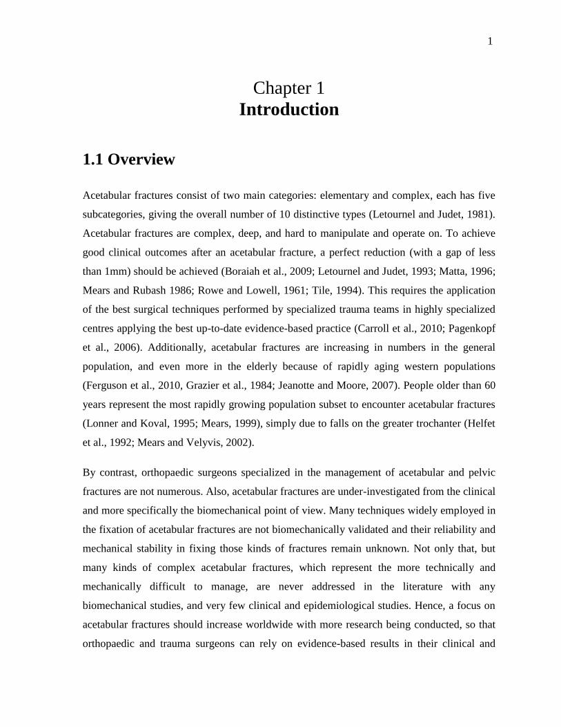
1.1 Overview

Acetabular fractures consist of two main categories: elementary and complex, each has five

subcategories, giving the overall number of 10 distinctive types (Letournel and Judet, 1981).

Acetabular fractures are complex, deep, and hard to manipulate and operate on. To achieve

good clinical outcomes after an acetabular fracture, a perfect reduction (with a gap of less

than 1mm) should be achieved (Boraiah et al., 2009; Letournel and Judet, 1993; Matta, 1996;

Mears and Rubash 1986; Rowe and Lowell, 1961; Tile, 1994). This requires the application

of the best surgical techniques performed by specialized trauma teams in highly specialized

centres applying the best up-to-date evidence-based practice (Carroll et al., 2010; Pagenkopf

et al., 2006). Additionally, acetabular fractures are increasing in numbers in the general

population, and even more in the elderly because of rapidly aging western populations

(Ferguson et al., 2010, Grazier et al., 1984; Jeanotte and Moore, 2007). People older than 60

years represent the most rapidly growing population subset to encounter acetabular fractures

(Lonner and Koval, 1995; Mears, 1999), simply due to falls on the greater trochanter (Helfet

et al., 1992; Mears and Velyvis, 2002).

By contrast, orthopaedic surgeons specialized in the management of acetabular and pelvic

fractures are not numerous. Also, acetabular fractures are under-investigated from the clinical

and more specifically the biomechanical point of view. Many techniques widely employed in

the fixation of acetabular fractures are not biomechanically validated and their reliability and

mechanical stability in fixing those kinds of fractures remain unknown. Not only that, but

many kinds of complex acetabular fractures, which represent the more technically and

mechanically difficult to manage, are never addressed in the literature with any

biomechanical studies, and very few clinical and epidemiological studies. Hence, a focus on

acetabular fractures should increase worldwide with more research being conducted, so that

orthopaedic and trauma surgeons can rely on evidence-based results in their clinical and

2

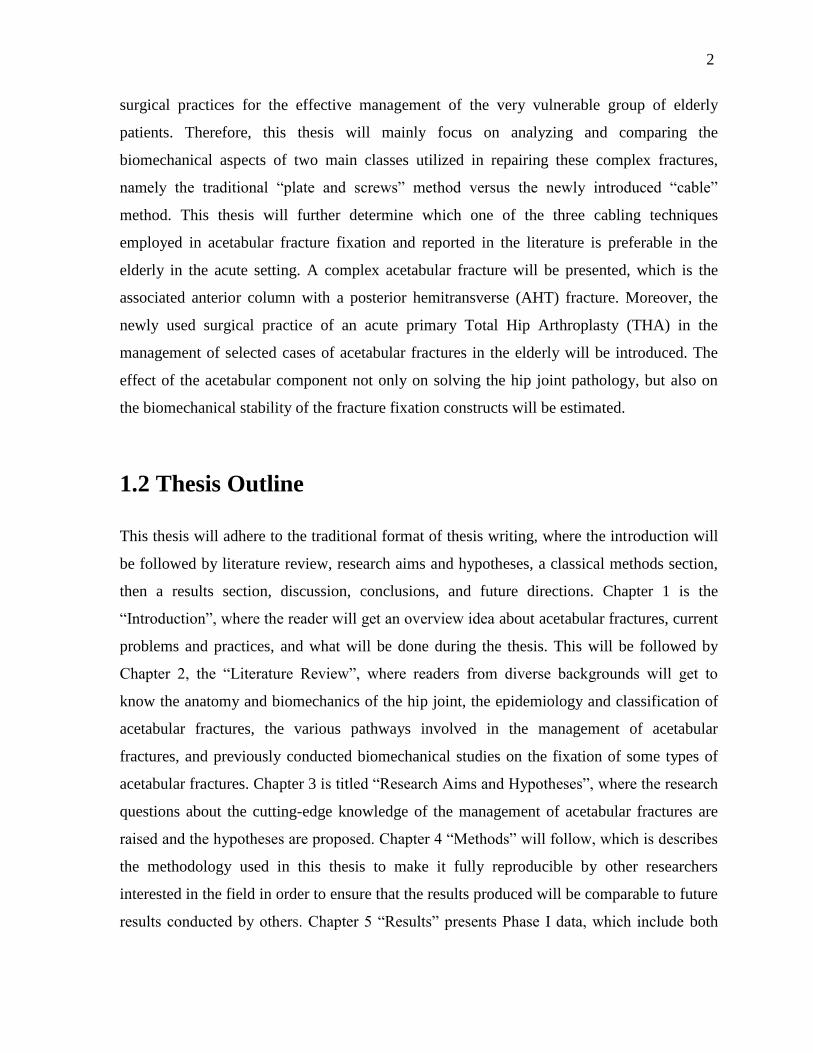
surgical practices for the effective management of the very vulnerable group of elderly

patients. Therefore, this thesis will mainly focus on analyzing and comparing the

biomechanical aspects of two main classes utilized in repairing these complex fractures,

namely the traditional “plate and screws” method versus the newly introduced “cable”

method. This thesis will further determine which one of the three cabling techniques

employed in acetabular fracture fixation and reported in the literature is preferable in the

elderly in the acute setting. A complex acetabular fracture will be presented, which is the

associated anterior column with a posterior hemitransverse (AHT) fracture. Moreover, the

newly used surgical practice of an acute primary Total Hip Arthroplasty (THA) in the

management of selected cases of acetabular fractures in the elderly will be introduced. The

effect of the acetabular component not only on solving the hip joint pathology, but also on

the biomechanical stability of the fracture fixation constructs will be estimated.

1.2 Thesis Outline

This thesis will adhere to the traditional format of thesis writing, where the introduction will

be followed by literature review, research aims and hypotheses, a classical methods section,

then a results section, discussion, conclusions, and future directions. Chapter 1 is the

“Introduction”, where the reader will get an overview idea about acetabular fractures, current

problems and practices, and what will be done during the thesis. This will be followed by

Chapter 2, the “Literature Review”, where readers from diverse backgrounds will get to

know the anatomy and biomechanics of the hip joint, the epidemiology and classification of

acetabular fractures, the various pathways involved in the management of acetabular

fractures, and previously conducted biomechanical studies on the fixation of some types of

acetabular fractures. Chapter 3 is titled “Research Aims and Hypotheses”, where the research

questions about the cutting-edge knowledge of the management of acetabular fractures are

raised and the hypotheses are proposed. Chapter 4 “Methods” will follow, which is describes

the methodology used in this thesis to make it fully reproducible by other researchers

interested in the field in order to ensure that the results produced will be comparable to future

results conducted by others. Chapter 5 “Results” presents Phase I data, which include both

3

experimental testing and FEA, and Phase II data, which compare the standard fixation

method using plate/screw versus the best cable method until mechanical failure. Chapter 6

“Discussion” is the main section interpreting the results and discussing important findings on

the fixation of complex acetabular fractures in the elderly. Chapter 7 “Conclusions” shortly

explains the main outcomes of the current study in brief “take-home” messages. Chapter 8

“Future Directions” shows how the current study can be related to and followed by coming

significant studies about the fixation of other complex acetabular fractures in the elderly

employing currently applied surgical techniques and procedures.

4

Chapter 2

Literature Review (Background)

2.1 Anatomy of the Hip

2.1.1 Descriptive Anatomy of the Hip

2.1.1.1 Hip Bone

The hip bone, also called Innominate bone, Pelvic bone, or Coxal bone (Gray, 2000) is

formed of three separate bones, namely the Ilium, Ischium, and Pubis, that unite together

over time until it is completely united in adulthood (Fig. 2.1 and 2.2). This union of the bones

forms the Acetabulum in the middle of the hip bone. The two hip bones, specifically the

Pubic bones, meet anteriorly in the midline of the body at the Symphysis Pubis and both

bones, namely Iliac bones, unite posteriorly with the sacrum forming the pelvis region.

The Ilium is the biggest of the three bones and is the flat extended large superior bone. It

consists of two parts; the body and the ala, which are distinguished from each other by the

arcuate line on the inner surface and the margin of the acetabulum on the outer surface. The

body forms the roof i.e. the superior portion of the acetabulum, and is partly articular being

part of the Lunate surface of the acetabulum i.e. the horseshoe-shaped smooth region, and

partly non-articular consisting part of the Cotyloid Fossa i.e. the central inverted U-shaped

depressed region of the acetabulum. On the other hand, the ala consists of external and

internal surfaces, anterior and posterior borders, the iliac crest on top, and the acetabular

margin below. The characteristic features on the external surface are the three (anterior,

posterior, and inferior) gluteal lines, while on the internal surface, the iliac fossa and arcuate

line are the most important features. The iliac crest’s surface is broad and has outer and inner

lips with an intermediate line. The crest starts anteriorly with the Anterior Superior Iliac

Spine (ASIS) and ends posteriorly with the Posterior Superior Iliac Spine (PSIS), also it has

the gluteus medius tubercle about 5 cm posterior to the ASIS, on top of the anterior pillar.

5

The Ischium is the hardest, lowermost, backmost bone of the three. It consists of a body, a

superior ramus, and an inferior ramus. The body unties with the other two bones to form the

acetabulum and participated into just more than 40% of the acetabulum; forming partly the

lunate surface and partly the posterior portion of the Cotyloid fossa. From the body protrudes

a thin elongated triangular projection, the Ischial spine, to which some muscles are attached.

Above the ischial spine, a large notch is found, the Greater Sciatic Notch (GSN), which is

converted into foramen by the attachment of the Sacrospinous ligament. The GSN transmits

many important structures, such as the superior and inferior gluteal vessels and nerves, the

Sciatic and posterior femoral cutaneous nerves, and the pyriformis. Below the spine, there is

a smaller notch called the Lesser Sciatic Notch (LSN), which is transformed into a foramen

by the Sacrotuberous and Sacrospinous ligaments. Through the LSN pass the internal

pudendal vessels and nerve as well as the obturator internus tendon and nerve. The superior

ramus originates from the body and is directed downwards and posteriorly until it ends as the

inferior ischial ramus. The posterior surface of the superior ramus forms a large protrusion

called the Ischial Tuberosity, which is divided into upper and lower parts by a transverse

ridge. The lower part gives origin to the Adductor Magnus muscle and Sacrotuberous

ligament, while the upper part gives origin to the Semimembranosus, long head of the Biceps

Femoris, and Semitendinosus. The inferior ramus is thin and flat, extending from the superior

ischial ramus to the inferior pubic ramus, where it joins with the latter forming a raised ridge.

The Pubis is the smallest and anteriormost bone of the three bones forming the hip. It

consists of a body, a superior ramus, and an inferior ramus. The body, as in the previous two

bones, attributes to the formation of the acetabulum representing 20% of it. The body is

involved in both the lunate surface and the Cotyloid Fossa. The superior ramus extends

anteriorly and medially from the body and is divided into two smaller parts, namely a medial

flat portion, and a lateral prismoid portion. The medial portion has a large tubercle protruding

anteriorly; the Pubic Tubercle, to which the inguinal ligament is medially attached. The

superior surface of the lateral portion has a rough ridge, the Iliopectineal eminence, which

represents the place of junction between the ilium and pubis.

6

Fig. 2.1: Lateral view of the hip bone showing all the characteristic features, which will

be referred to during the whole thesis (Gray, 2000).

Fig. 2.2: Medial view of the hip bone demonstrating the important features, which will

be referred to during the whole thesis (Gray, 2000).

7

2.1.1.2 Acetabulum

The acetabulum is a central hemispherical depression in the middle of the hip bone; formed

by the union of the bodies of the three bones forming the hip bone, namely the ilium,

ischium, and pubis (Fig. 2.3) (Gray, 2000). The body of the ilium forms just less than 40% of

the acetabulum; the body of the ischium forms a little more than 40% of the acetabulum,

while the pubic body constitutes the remaining 20% of the acetabulum. The acetabular

surface has two important parts; the lunate surface and the acetabular (Cotyloid) fossa. The

lunate surface is the articular region and it has a horseshoe-like shape, while the cotyloid

fossa is a central inverted U-shaped depression, connected below to the acetabular notch. The

acetabulum, being a hemisphere, has a rim all around except inferiorly, where the rim is

missing and the acetabular notch is present. The rim is most prominent and strongest

superiorly in the load-bearing region of the acetabulum and called the roof of the acetabulum.

The roof is the area of articular surface that forms the arch of a 45-60° angle, extending from

the Anterior Inferior Iliac Spine (AIIS) anteriorly to the ilio-iscial notch of the acetabular

margin posteriorly. To the rim is attached the glenoidal labrum, which is a circular ligament,

further deepening and narrowing the articular surface between the femoral head and

acetabulum. The acetabular notch is converted into a foramen by the transverse ligament,

through which nutrient vessels and nerves penetrate the joint.

8

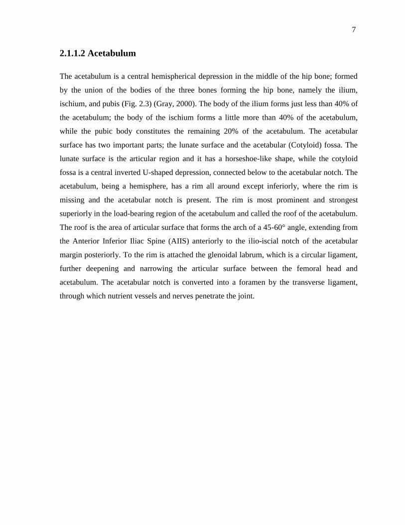
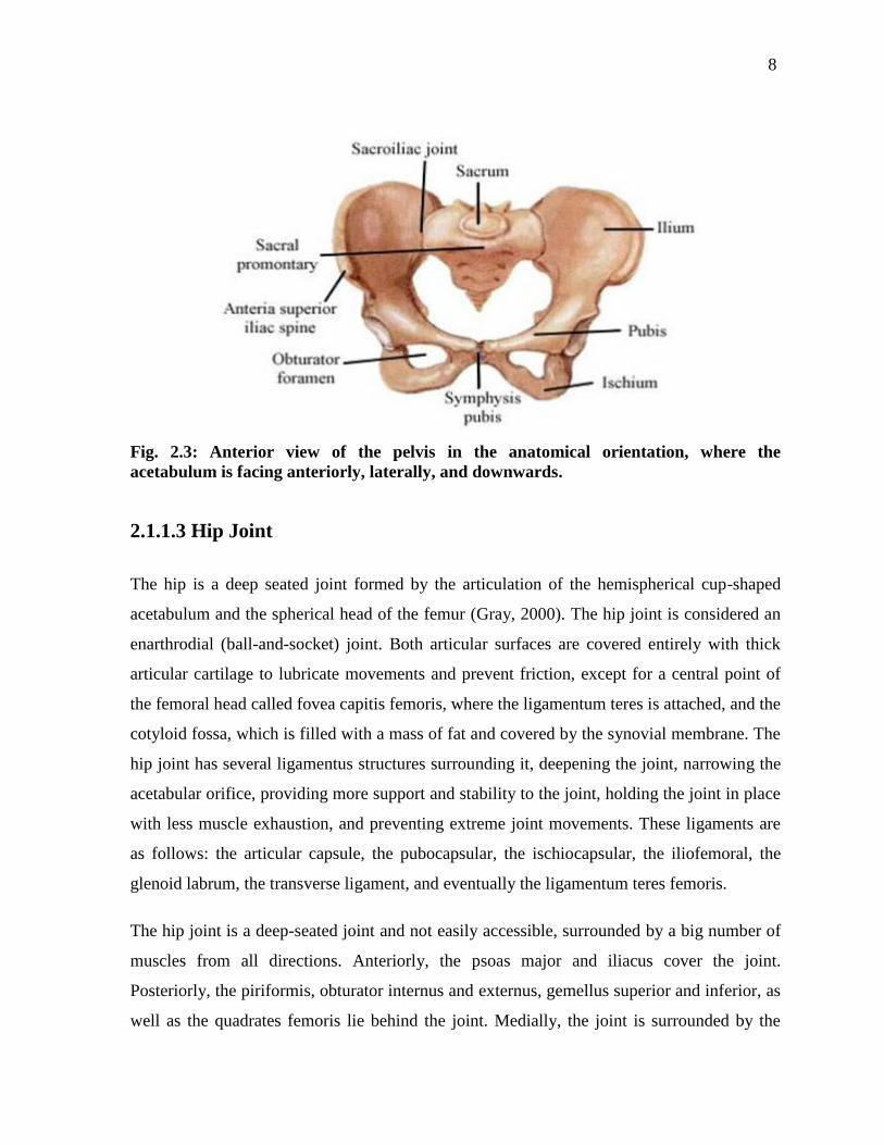
Fig. 2.3: Anterior view of the pelvis in the anatomical orientation, where the

acetabulum is facing anteriorly, laterally, and downwards.

2.1.1.3 Hip Joint

The hip is a deep seated joint formed by the articulation of the hemispherical cup-shaped

acetabulum and the spherical head of the femur (Gray, 2000). The hip joint is considered an

enarthrodial (ball-and-socket) joint. Both articular surfaces are covered entirely with thick

articular cartilage to lubricate movements and prevent friction, except for a central point of

the femoral head called fovea capitis femoris, where the ligamentum teres is attached, and the

cotyloid fossa, which is filled with a mass of fat and covered by the synovial membrane. The

hip joint has several ligamentus structures surrounding it, deepening the joint, narrowing the

acetabular orifice, providing more support and stability to the joint, holding the joint in place

with less muscle exhaustion, and preventing extreme joint movements. These ligaments are

as follows: the articular capsule, the pubocapsular, the ischiocapsular, the iliofemoral, the

glenoid labrum, the transverse ligament, and eventually the ligamentum teres femoris.

The hip joint is a deep-seated joint and not easily accessible, surrounded by a big number of

muscles from all directions. Anteriorly, the psoas major and iliacus cover the joint.

Posteriorly, the piriformis, obturator internus and externus, gemellus superior and inferior, as

well as the quadrates femoris lie behind the joint. Medially, the joint is surrounded by the

9

obturator extenus and pectineus. Above and laterally, there are the long head of the rectus

femoris and the gluteus minimus. The joint has vascular supply from the peri-acetabular

circle formed by multiple nutrient vessels along the acetabular margin, namely the obturator

artery, inferior gluteal artery, artery of the roof which is a branch of the superior gluteal

artery, plus other local nutrient branches. The joint receive sensory nerve supply from the

sacral plexus, sciatic, obturator, and accessory obturator nerves.

2.1.1.4 Hip Muscles and Movements

The hip joint is a multi-axial ball-and-socket joint, and therefore, movements along

perpendicular planes occur over a wide arch of motion, namely flexion and extension,

adduction and abduction, medial and lateral rotation, and circumduction (Gray, 2000).

Muscles surrounding the hip are divided into groups; each is mainly, but not only,

responsible for a certain movement of the hip. The main hip flexor is the psoas muscle,

helped by the iliacus, but also other muscles assist in hip flexion. Extension is mainly

performed by the gluteus maximus. Adduction is mainly carried out by the adductor group of

muscles, such as the adductor brevis, longus, and magnus. Hip abduction is mainly exerted

by the gluteus medius and minimus. Medial rotation usually occurs by the action of glutei

medius and minimus, tensor fasciae latae and the adductors, while lateral rotation is primarily

performed by the lateral rotator group, such as the obturators internus and externus, gemelli

superior and inferior, and the quadratus femoris. Hip muscles coordinate together to achieve

successful hip movement, and hold the position of the pelvic girdle during standing. Also,

they integrate in action with neck, shoulder, trunk, and leg muscles to maintain position of

the body and maximize stability.

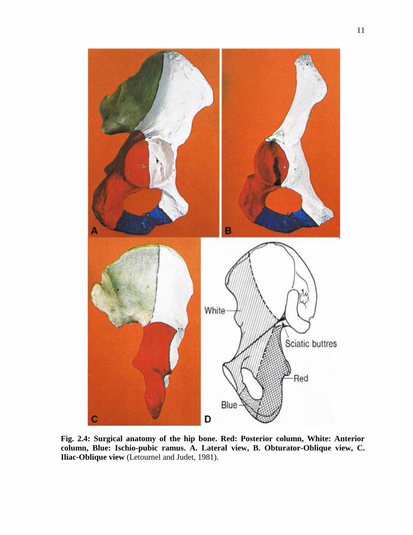
2.1.2 Surgical Anatomy of the Hip

According to Letournel and Judet (1981), the acetabulum is looked at as being seated within

the open arms of an inverted Y-structure (Fig. 2.4). This structure represents both the anterior

and posterior columns of the acetabulum. The anterior column is much longer than the

10

posterior one and extends from the anterior portion of the iliac crest superiorly all the way

down to the Symphysis Pubis (SP), while the posterior column travels from the lowermost

end of the ischium to meet with the posterior aspect of the anterior column just above its

mid-point, almost at the level of the upper corner of the GSN, creating a 60° angle. The

acetabulum is enclosed within this angle and the apex is filled with condense cortical bone

forming the roof for the acetabulum.

The posterior column, also called ilio-ischial column, is triangular in the cross section and is

formed of an internal, posterior and antero-lateral surfaces. The internal surface forms the

posterior portion of the quadrilateral plate. The posterior surface forms part of the posterior

wall of the acetabulum and the subcotyloid groove for the tendon of the obturator externus

above and the ischial tuberosity below. The antero-lateral surface represents the posterior

portion of the articular surface of the acetabulum above, and the body of the ischium below.

The posterior border of the posterior column consists of the ilium above, the GSN in the

middle, and then the LSN below.

The Anterior column contains the iliac, acetabular, and pubic segments. The iliac segment

extends from the iliac crest superiorly to just above the acetabular margin. Its main features

are the anterior pillar, ASIS and Anterior Inferior Iliac Spine (AIIS), which is very close to

the superior margin of the acetabulum. The acetabular segment forms the anterior articular

surface of the acetabulum, part of the anterior wall of the acetabulum, and the anterior

portion of the quadrilateral plate of the acetabulum. The pubic segment constitutes the

anteriormost, and slimmest portion of the anterior column, and consists of the superior pubic

ramus forming the roof to the obturator foramen. The iliopectineal line is a fundamental

structure of the anterior column providing support to the anterio-superior aspect of the

acetabulum and is the main guide for evaluating the continuity of the anterior column.

Fractures of this line usually indicate fractures of the anterior column. Both columns are

connected to the auricular surface of the Sacro-iliac (SI) joint by the sciatic buttress.

11

Fig. 2.4: Surgical anatomy of the hip bone. Red: Posterior column, White: Anterior

column, Blue: Ischio-pubic ramus. A. Lateral view, B. Obturator-Oblique view, C.

Iliac-Oblique view (Letournel and Judet, 1981).

12

2.2 Biomechanics of the Hip

2.2.1 Overview

Force can be transmitted from the head of the femur to the acetabulum causing acetabular

fractures and/or dislocation of the femoral head, when the force is high enough to cause this

and applied in any of four locations, namely the greater trochanter of the femur, the flexed

knee, the foot (when the knee is extended), and posteriorly on the pelvis (Letournel and

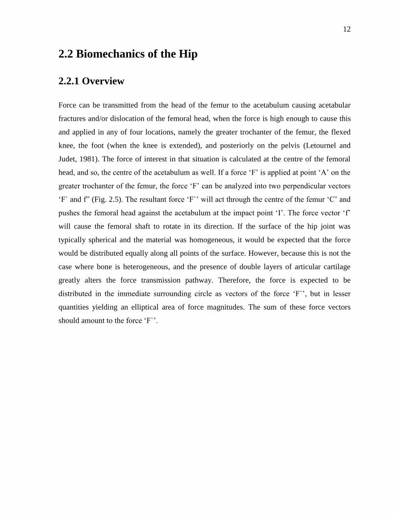
Judet, 1981). The force of interest in that situation is calculated at the centre of the femoral

head, and so, the centre of the acetabulum as well. If a force ‘F’ is applied at point ‘A’ on the

greater trochanter of the femur, the force ‘F’ can be analyzed into two perpendicular vectors

‘F` and f” (Fig. 2.5). The resultant force ‘F`’ will act through the centre of the femur ‘C’ and

pushes the femoral head against the acetabulum at the impact point ‘I’. The force vector ‘f’

will cause the femoral shaft to rotate in its direction. If the surface of the hip joint was

typically spherical and the material was homogeneous, it would be expected that the force

would be distributed equally along all points of the surface. However, because this is not the

case where bone is heterogeneous, and the presence of double layers of articular cartilage

greatly alters the force transmission pathway. Therefore, the force is expected to be

distributed in the immediate surrounding circle as vectors of the force ‘F`’, but in lesser

quantities yielding an elliptical area of force magnitudes. The sum of these force vectors

should amount to the force ‘F`’.

13

Fig. 2.5: Free body diagram of force (F) acting on the greater trochanter at point (A)

transmitting a net force (F’) through the centre of the femoral head (C), yielding an

impact on the acetabulum at point (I), with an ellipse of influence (shaded area)

(Letournel and Judet, 1981).

2.2.2 Force Applied to the Greater Trochanter

In this condition, only the rotational (internal vs. external) and abductory/adductory

movements of the hip have a big impact on the location of force impact on the acetabulum,

and hence, on the fracture pattern. However, flexion/extension plays only a minimal role.

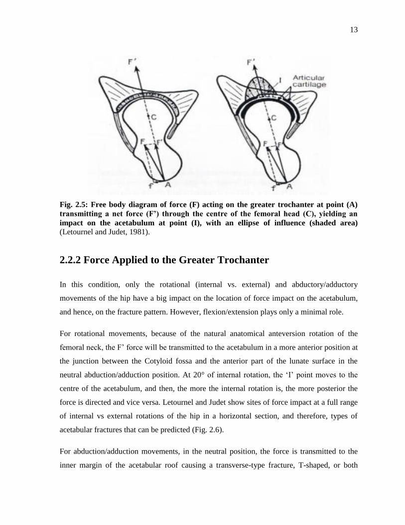
For rotational movements, because of the natural anatomical anteversion rotation of the

femoral neck, the F’ force will be transmitted to the acetabulum in a more anterior position at

the junction between the Cotyloid fossa and the anterior part of the lunate surface in the

neutral abduction/adduction position. At 20° of internal rotation, the ‘I’ point moves to the

centre of the acetabulum, and then, the more the internal rotation is, the more posterior the

force is directed and vice versa. Letournel and Judet show sites of force impact at a full range

of internal vs external rotations of the hip in a horizontal section, and therefore, types of

acetabular fractures that can be predicted (Fig. 2.6).

For abduction/adduction movements, in the neutral position, the force is transmitted to the

inner margin of the acetabular roof causing a transverse-type fracture, T-shaped, or both

14

column fractures. The more the adduction is, the more superior the force travels causing

transverse fractures at the acetabular roof, and vice versa, the more the abduction is, the

higher the possibility to encounter a fracture below the articular surface of the acetabular roof

and is transversely placed.

Fig. 2.6: A. Transverse section through the hip joint showing the effect of different

degrees of internal/external rotation of the femur on locations of force transmission. B.

Coronal section of the hip joint at 20° of internal rotation illustrating the effect of

different abduction/adduction on the lines of force transmission (Letournel and Judet,

1981).

2.2.3 Force Applied to the Flexed Knee

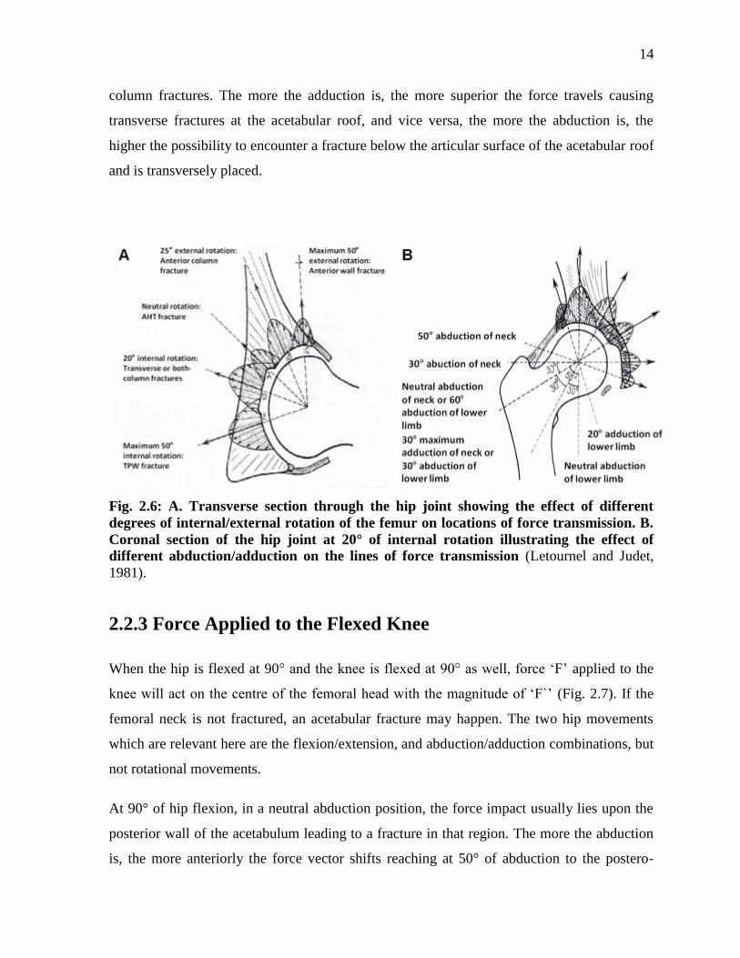
When the hip is flexed at 90° and the knee is flexed at 90° as well, force ‘F’ applied to the

knee will act on the centre of the femoral head with the magnitude of ‘F`’ (Fig. 2.7). If the

femoral neck is not fractured, an acetabular fracture may happen. The two hip movements

which are relevant here are the flexion/extension, and abduction/adduction combinations, but

not rotational movements.

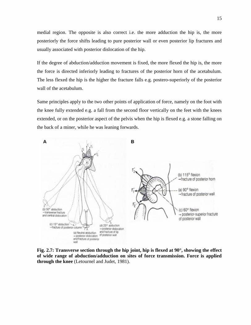
At 90° of hip flexion, in a neutral abduction position, the force impact usually lies upon the

posterior wall of the acetabulum leading to a fracture in that region. The more the abduction

is, the more anteriorly the force vector shifts reaching at 50° of abduction to the postero-

15

medial region. The opposite is also correct i.e. the more adduction the hip is, the more

posteriorly the force shifts leading to pure posterior wall or even posterior lip fractures and

usually associated with posterior dislocation of the hip.

If the degree of abduction/adduction movement is fixed, the more flexed the hip is, the more

the force is directed inferiorly leading to fractures of the posterior horn of the acetabulum.

The less flexed the hip is the higher the fracture falls e.g. postero-superiorly of the posterior

wall of the acetabulum.

Same principles apply to the two other points of application of force, namely on the foot with

the knee fully extended e.g. a fall from the second floor vertically on the feet with the knees

extended, or on the posterior aspect of the pelvis when the hip is flexed e.g. a stone falling on

the back of a miner, while he was leaning forwards.

Fig. 2.7: Transverse section through the hip joint, hip is flexed at 90°, showing the effect

of wide range of abduction/adduction on sites of force transmission. Force is applied

through the knee (Letournel and Judet, 1981).

16

2.3 Acetabular Fractures

2.3.1 Epidemiology

2.3.1.1 Incidence and Prevalence

According to the “Fracture and Dislocation Classification Compendium 2007” executed by

the “Orthopaedic Trauma Association – Classification, Database and Outcomes Committee”

(Marsh et al., 2007), pelvic fractures (#6) are divided into pelvic ring (#61) and acetabular

(#62) fractures. First, there are not much data on the exact epidemiology (incidence and

prevalence) of pelvic fractures in general, and specifically pelvic ring and acetabular

fractures. Furthermore, the literature is severely lacking enough information about the

incidence and prevalence of specific types of acetabular fractures in different parts of the

world. Second, the records and studies provided for pelvic fractures in Europe, especially the

UK, are totally different from those provided for North America (Court-Brown et al., 2006,

2010), leading to the conclusion that the incidence and prevalence of pelvic fractures vary

from one region and country to the other region and country, specifically between the UK

and USA, where pelvic fractures take two totally different trends, distribution curves,

incidences and prevalences.

According to Court-Brown et al. (2006, 2010), the authors chose the fracture population to be

the Royal Infirmary of Edinburgh, Scotland because it is the only hospital that deals with

orthopaedic trauma in a confined population. The overall prevalence of pelvic fractures

represented about 2% of all types of fractures occurring in humans. In a comparison of their

databases provided in the years 2000 vs 2007/8, the prevalence of pelvic fractures increased

from 1.5% to 1.8% and the incidence increased by 46%. Also, acetabular fractures, unlike

pelvic ring fractures, occur in a relatively younger age, with an average of 58 years, are more

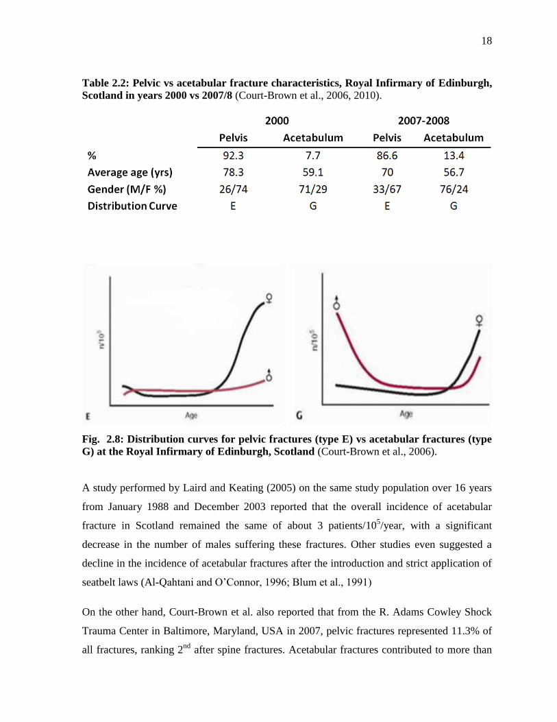
predominant in males than females 74/26, and follow a type G distribution curve (Fig. 2.8).

Type G curve demonstrates a unimodal increase in older females and a bimodal increase in

younger and older males with a flat low plateau in the middle age. A complete comparison

between the two studies is shown (Tables 2.1, 2.2). The Scotland database shows that

acetabular fractures constituted 7.7% in 2000 and almost doubled i.e. 13.4% in 2007/8 of all

17

pelvic fractures, with an obvious male predominance of 71% in 2000 and 76% in 2007/8 and

with an average age of 59.1 in 2000 to 56.7 in 2007/8. This shows a two-fold tendency of

acetabular fractures to increase: first, because of the overall increase in prevalence and

incidence of pelvic fractures, and second, because of the big increase in their percentage with

respect to pelvic fractures. The German Pelvic Study Group 2 (German Trauma Association

– Association for Osteosynthesis) reported that acetabular fractures represented 14% of all

pelvic fractures in the elderly population over 65 years (Culemann et al., 2010).

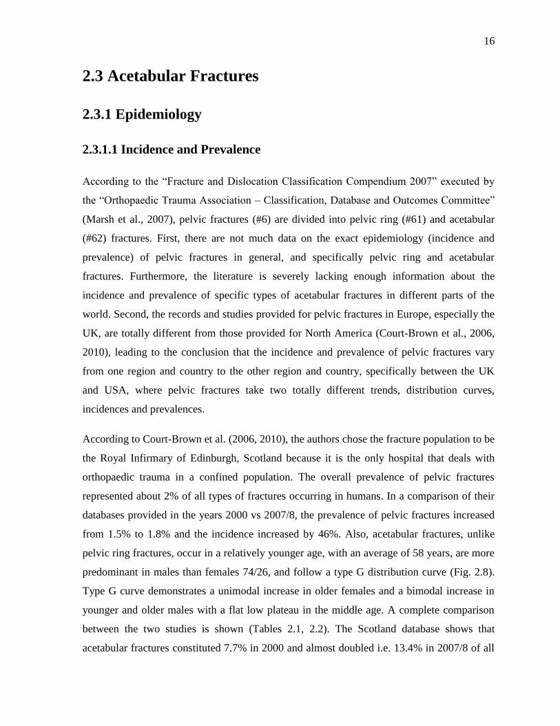
Table 2.1: Pelvic fracture characteristics, obtained from Royal Infirmary of Edinburgh,

Scotland in years 2000 vs 2007/8 (Court-Brown et al., 2006, 2010).

18

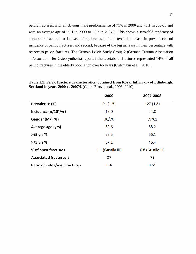
Table 2.2: Pelvic vs acetabular fracture characteristics, Royal Infirmary of Edinburgh,

Scotland in years 2000 vs 2007/8 (Court-Brown et al., 2006, 2010).

Fig. 2.8: Distribution curves for pelvic fractures (type E) vs acetabular fractures (type

G) at the Royal Infirmary of Edinburgh, Scotland (Court-Brown et al., 2006).

A study performed by Laird and Keating (2005) on the same study population over 16 years

from January 1988 and December 2003 reported that the overall incidence of acetabular

fracture in Scotland remained the same of about 3 patients/105/year, with a significant

decrease in the number of males suffering these fractures. Other studies even suggested a

decline in the incidence of acetabular fractures after the introduction and strict application of

seatbelt laws (Al-Qahtani and O’Connor, 1996; Blum et al., 1991)

On the other hand, Court-Brown et al. also reported that from the R. Adams Cowley Shock

Trauma Center in Baltimore, Maryland, USA in 2007, pelvic fractures represented 11.3% of

all fractures, ranking 2nd

after spine fractures. Acetabular fractures contributed to more than

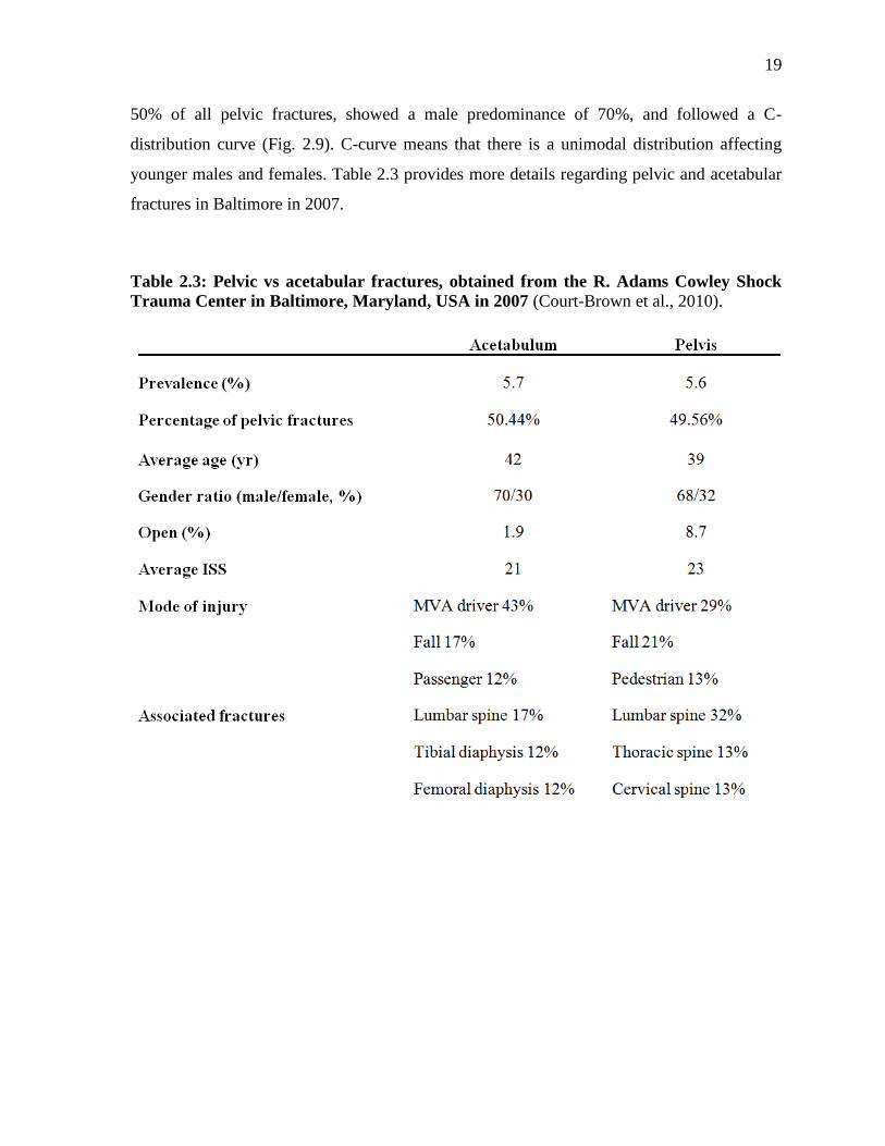
19

50% of all pelvic fractures, showed a male predominance of 70%, and followed a C-

distribution curve (Fig. 2.9). C-curve means that there is a unimodal distribution affecting

younger males and females. Table 2.3 provides more details regarding pelvic and acetabular

fractures in Baltimore in 2007.

Table 2.3: Pelvic vs acetabular fractures, obtained from the R. Adams Cowley Shock

Trauma Center in Baltimore, Maryland, USA in 2007 (Court-Brown et al., 2010).

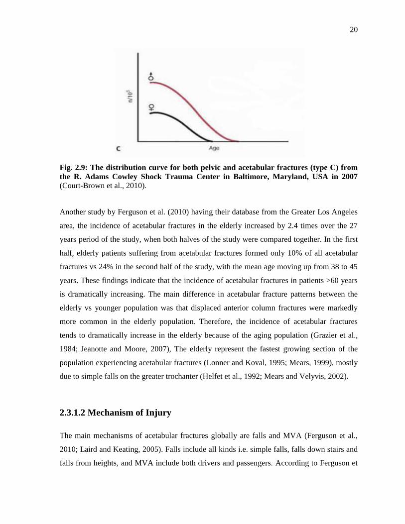
20

Fig. 2.9: The distribution curve for both pelvic and acetabular fractures (type C) from

the R. Adams Cowley Shock Trauma Center in Baltimore, Maryland, USA in 2007

(Court-Brown et al., 2010).

Another study by Ferguson et al. (2010) having their database from the Greater Los Angeles

area, the incidence of acetabular fractures in the elderly increased by 2.4 times over the 27

years period of the study, when both halves of the study were compared together. In the first

half, elderly patients suffering from acetabular fractures formed only 10% of all acetabular

fractures vs 24% in the second half of the study, with the mean age moving up from 38 to 45

years. These findings indicate that the incidence of acetabular fractures in patients >60 years

is dramatically increasing. The main difference in acetabular fracture patterns between the

elderly vs younger population was that displaced anterior column fractures were markedly

more common in the elderly population. Therefore, the incidence of acetabular fractures

tends to dramatically increase in the elderly because of the aging population (Grazier et al.,

1984; Jeanotte and Moore, 2007), The elderly represent the fastest growing section of the

population experiencing acetabular fractures (Lonner and Koval, 1995; Mears, 1999), mostly

due to simple falls on the greater trochanter (Helfet et al., 1992; Mears and Velyvis, 2002).

2.3.1.2 Mechanism of Injury

The main mechanisms of acetabular fractures globally are falls and MVA (Ferguson et al.,

2010; Laird and Keating, 2005). Falls include all kinds i.e. simple falls, falls down stairs and

falls from heights, and MVA include both drivers and passengers. According to Ferguson et

21

al., a fall is the most important mechanism of injury in the elderly representing 49.8% of all

causes, followed by MVA signifying 37.4%. While in the younger population, the number

one cause of injury was MVA causing 66% of all fractures, followed by fall, which

represented 17.7%. Laird and Keating also reported similar results showing that fall and

MVA are the two most significant causes of acetabular injuries, where falls caused 40.2%

and MVA contributed to 38.2% of fractures at all ages. Other causes of injury included bikes,

pedestrian versus auto, gun-shot wound, crush injuries, and sports.

2.3.2 Classification

2.3.2.1 History of Acetabular Fracture Classification

Before 1951 and for a long time thereafter, the traditional classification of acetabular

fractures was of two broad categories: either central dislocation, or posterior hip dislocation

with an acetabular fracture (Letournel and Judet, 1981). Cauchoix and Truchet in 1951 used

the above classification, but were not satisfied with it and added two more categories, namely

posterior wall acetabular fractures associated with a central dislocation, and trans-acetabular

fractures of the pelvis with posterior hip dislocation. This classification was insufficient to

explain the mechanisms causing acetabular fractures because any force between the femoral

ball and the acetabulum may cause posterior or central dislocation of the femoral head with

countless number of different possibilities for acetabular fractures that cannot be accounted

for. In 1961, Creyssel and Schnepp used the above-mentioned classification and tried to

distinguish principal and accessory fracture lines, and they used the term “trans-acetabular”

to describe transverse acetabular fractures. This classification system was rejected because

any fracture passing through the acetabulum is of the same importance and cannot be

considered “principal” or “accessory”. Also, the term “trans-acetabular” was not an accurate

description of transverse fractures because any fracture crossing the acetabulum can literally

be named “trans-acetabular”. Since 1960, Letournel and Judet created the current widely

used classification of acetabular fractures. The authors kept modifying their classification

since then to include all types of acetabular fractures, referring mainly to the essential

22

structure of the anterior and posterior columns holding the acetabulum in place, and ignoring

the femoral head displacement in their classification of fractures.

2.3.2.2 Current Acetabular Fracture Classification

Elementary Acetabular Fractures

Elementary acetabular fractures include these kinds of fractures which affect in part or in

total any of the two columns that support the acetabulum, namely fractures of the posterior

wall of the acetabulum, fractures of the posterior column, fractures of the anterior wall of the

acetabulum, and fractures of the anterior column (Letournel and Judet, 1981). The authors

added to them the transverse fracture, being a single fracture passing transversely through

both columns of the acetabulum, but not associated with any other fractures.

Associated Acetabular Fractures

The associated fractures mean that they have at least two of the above mentioned elementary

fractures. There are five types of associated acetabular fractures: T-shaped fractures,

fractures of the posterior column and posterior wall, transverse and posterior fractures,

fractures of the anterior column or anterior wall with posterior hemitransverse fracture, and

both-column fractures (Letournel and Judet, 1981).

2.4 Associated Anterior and Posterior Hemitransverse

Fractures

2.4.1 Nomenclature

This associated fracture type was named so because it involves two components: an anterior

component, which mainly includes the anterior column. But it may also affect only the

23

anterior wall, and a posterior component, which typically resembles the posterior half of a

transverse fracture. This is the reason for the term “posterior hemitransverse fracture”.

2.4.2 Incidence

Not much data exist in the literature to determine the exact contribution of the anterior with

posterior hemitransverse (AHT) to the overall incidence of acetabular fractures. However,

only two detailed epidemiological studies about acetabular fractures including the detailed

characterization into each of the 10 elementary and associated types, are available in the

literature. One was performed by Laird and Keating in the UK, and the other one was done

by Ferguson et al. in North America. The latter showed that the fracture type of interest was a

common fragility fracture occurring in the elderly and represented 15% of all types of

acetabular fractures and about 25% of associated acetabular fractures (Ferguson et al., 2010).

However, Laird and Keating reported in their study that this fracture type caused only 6.7%

of all acetabular fractures, and 15% of associated acetabular fractures (Laird and Keating,

2005). However, the two populations are totally different as noticed from other parameters

mentioned before, and also Ferguson et al.’s study is much larger for two reasons; first, it

was run over a period of 27 years vs only 16 years, and second, total number of patients

involved was 1309 (all classified into the 10 different types except 14 cases (1.3%) were

unknown) vs 351 (of them, only 163 were classified and 188 (53.6%) not classified). Another

study stated that the anterior column combined with posterior hemitransverse fracture was

particularly common in the elderly (Hessmann et al., 2002), and therefore, this kind of

acetabular fractures is usually considered the typical acetabular fracture in the elderly

(Culemann et al., 2010).

24

2.4.3 Morphology

2.4.3.1 Anterior Component

The anterior component of the AHT associated fracture can be either an anterior wall fracture

(less common) or an anterior column fracture (more common) (Fig. 2.10) (Letournel and

Judet, 1981). If it is an anterior wall fracture, it will have the typical features of anterior wall

fractures, where the broken segment can be fully separated or remain in contact with the

superior pubic ramus. Infrequently, there may be an associated fracture at the ischio-pubic

ramus, or an elevation of the cortex from the quadrilateral plate displaced medially by the

femoral head.

If it is an anterior column fracture, which is usually the case, it can be considered as an

elementary anterior column fracture, and divided into four categories:

1) Low anterior column fracture, where the fracture line ruptures from the psoas groove

just inferior to the AIIS.

2) Intermediate anterior column fracture, where the fracture line exits from the anterior

border of the iliac wing somewhere in between the ASIS and AIIF.

3) High complete anterior column fracture, where the fracture ruptures through the iliac

crest.

4) High incomplete anterior column fracture, where the fracture line does not go all the

way up to the iliac crest, but is directed in that direction.

In either case, the displacement of the anterior component is always severe and associated

with anterior dislocation of the femoral head. Also, the anterior component can be looked at

as being a pure anterior fracture and considered to be independent of the posterior

component.

25

2.4.3.2 Posterior Component

The posterior component can be regarded as a posterior half of the elementary transverse

fracture (Fig. 2.10) (Letournel and Judet, 1981). The fracture line may cross the posterior

column of the pelvis at any level. The posterior border of the acetabulum can be traversed by

the acetabulum in its inferior quarter or below (most likely), in the middle, or through the

upper part. Then, the fracture line crosses the anterior border of the GSN at any level from

the superior border, to even splitting the ischial spine. The displacement of the posterior

column is much less remarkable than that of the anterior counterpart. This component usually

cuts the retro-acetabular portion of the posterior column obliquely from medial to lateral,

then crosses perfectly transverse through the posterior column until it cuts the anterior

component at a right angle. Occasionally, the posterior fracture may not split the posterior

column completely and stop before the dense anterior border of the GSN. This kind of

fracture is then regarded as an intermediary stage between pure anterior column fracture and

the associated AHT.

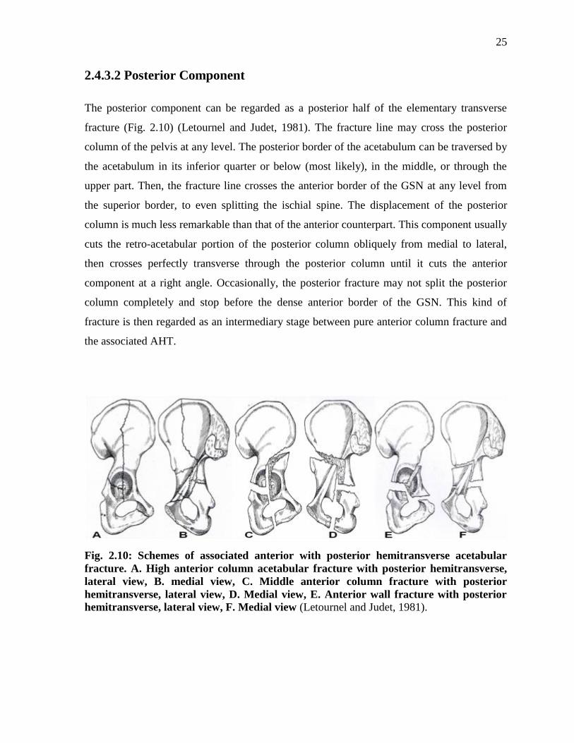
Fig. 2.10: Schemes of associated anterior with posterior hemitransverse acetabular

fracture. A. High anterior column acetabular fracture with posterior hemitransverse,

lateral view, B. medial view, C. Middle anterior column fracture with posterior

hemitransverse, lateral view, D. Medial view, E. Anterior wall fracture with posterior

hemitransverse, lateral view, F. Medial view (Letournel and Judet, 1981).

26

2.5 Management of Acetabular Fractures

2.5.1 Overview

Early in the 20th

century, almost all treatments offered to acetabular fractures were only

conservative for the risk of operating on such difficult fracture types and also due to the risks

related to anaesthesia and other pre-operative medical comorbidities (Letournel and Judet,

1981). It was not until Letournel and Judet started to realize that there was tendency to over-

evaluate the outcomes of the conservative management and they decided to operatively

manage any acutely displaced acetabular fracture with an ORIF, which if achieved anatomic

reduction of the acetabular fracture, would lead to a big jump in the successful outcomes

after acetabular fractures. The goal of operative treatment of any acetabular fractures is to

achieve perfect anatomical reduction of the hip bone and the articular surface of the

acetabulum (Boraiah et al., 2009; Matta, 1996). The anatomical reduction is considered the

single most important factor for clinical success over the long-term follow-up (Letournel and

Judet, 1993; Mears and Rubash 1986; Rowe and Lowell, 1961; Tile, 1994). Lately in the last

20 to a maximum of 30 years, teams of orthopaedic surgeons specialized in the fixation of

acetabular fractures started performing the Combined Hip Procedure (CHP) which basically

means the simultaneous fixation of the fracture with an ORIF to provide a good bone-stock

and support to the acute primary THA performed at the same setting (Boraiah et al., 2009;

Herscovici et al., 2010; Mears and Velyvis, 2000; Mears and Velyvis, 2002; Mears et al.,

2003; Pagenkopf et al., 2006). Other options for the repair of acetabular fractures especially

in the elderly include minimally invasive percutaneous fixation of the fracture,

salvage/delayed primary THA after the conservative management failed yielding post-

traumatic osteoarthritis, bone deformity, mal-union or non-union, or even after ORIF due to

the development of post-traumatic osteoarthritis (Pagenkopf et al., 2003; Tidermark et al.,

2003; Vanderschot, 2007). The main goal of all methods of acetabular fracture fixation is to

provide a functional hip joint with or close to symptom-free with good to excellent clinical

outcomes. Currently, most orthopaedic teams specialized in acetabular fractures are more or

less in an agreement regarding the treatment of acetabular fractures in adults. However, in the

elderly, there are no clear directions or guidelines to guide orthopaedic surgeons make the

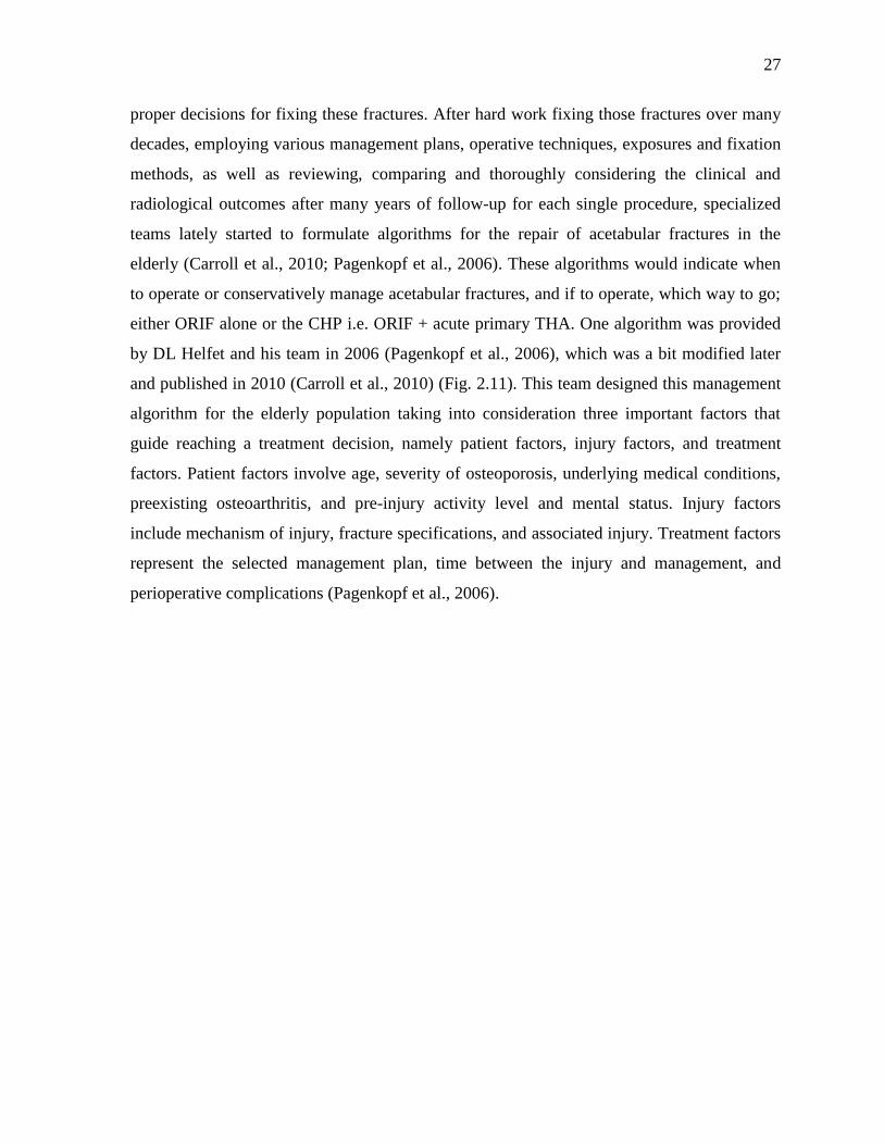
27

proper decisions for fixing these fractures. After hard work fixing those fractures over many

decades, employing various management plans, operative techniques, exposures and fixation

methods, as well as reviewing, comparing and thoroughly considering the clinical and

radiological outcomes after many years of follow-up for each single procedure, specialized

teams lately started to formulate algorithms for the repair of acetabular fractures in the

elderly (Carroll et al., 2010; Pagenkopf et al., 2006). These algorithms would indicate when

to operate or conservatively manage acetabular fractures, and if to operate, which way to go;

either ORIF alone or the CHP i.e. ORIF + acute primary THA. One algorithm was provided

by DL Helfet and his team in 2006 (Pagenkopf et al., 2006), which was a bit modified later

and published in 2010 (Carroll et al., 2010) (Fig. 2.11). This team designed this management

algorithm for the elderly population taking into consideration three important factors that

guide reaching a treatment decision, namely patient factors, injury factors, and treatment

factors. Patient factors involve age, severity of osteoporosis, underlying medical conditions,

preexisting osteoarthritis, and pre-injury activity level and mental status. Injury factors

include mechanism of injury, fracture specifications, and associated injury. Treatment factors

represent the selected management plan, time between the injury and management, and

perioperative complications (Pagenkopf et al., 2006).

28

Fig. 2.11: Algorithm for the management of acetabular fractures in the elderly,

developed by the specialized team of Helfet and co-workers (Carroll et al., 2010).

29

2.5.2 Conservative Treatment

2.5.2.1 Indications

Conservative management of acetabular fractures is mainly adopted in the following

conditions (Fig. 2.11) (Boraiah et al., 2009; Carroll et al., 2010; Gross et al., 1993;

Herscovici et al., 2010; Letournel and Judet, 1981; Mears and Rubash, 1986; Mears and

Velyvis, 2000; Pagenkopf et al., 2006):

1) Medical co-morbidities that make the risks to operate much higher than the benefits

the patient may achieve.

2) Immobility: because if the patient is immobile, even if the surgeon achieves perfect

reduction and fixation of the acetabulum, there will be no much gain for the patient.

3) Undisplaced, minimally-displaced, or stable fractures.

4) Pre-existing osteoarthritis or severe osteoporosis in a rather non-operable patient

rendering a successful reduction of the fracture hard to accomplish.

5) In some cases of both-column fractures with osteopenia, comminution, and

displacement if secondary congruency can be achieved by traction.

2.5.2.2 Methods

Usually bed rest with passive movements is encouraged in the beginning that increases with

time until walking with crutches can be accomplished at 6 weeks, followed by full weight-

bearing by 10 weeks (Letournel and Judet, 1981). Traction either skeletal or skin traction is

not really recommended in conservative management because it does not correct any

displacement, which is usually rotational and not translational (Matt et al., 1986;

Vanderschot, 2007). Also, using pins in the greater trochanter to apply traction usually fails

because of slippage out of the bone and also predisposes to local infections. Longitudinal

traction does not work as well. Manipulative reduction of a displaced femoral head is

mandatory to prevent avascular necrosis (Letournel and Judet, 1981; Vanderschot, 2007).

30

2.5.2.3 Complications

The conservative treatment may cause residual pelvic deformities because it does not reduce

the fracture. Therefore, occult or frank non-union or mal-union of the fracture may be the

ultimate result. Also, this way of management may lead to loss of the bone-stock of the

acetabulum, or the femoral head, resulting later in loosening of the implants installed in

salvage (delayed) THA. The radiological loosening rates reached 30% for femoral

components and 40-53% of acetabular components (Gross et al., 1993; Helfet et al., 1992;

Herscovici et al., 2010; Mears and Rubash, 1986; Mears and Velyvis, 2000; Romness and

Lewallen, 1990).

2.5.3 Surgical Treatment

2.5.3.1 Surgical Access

There are mainly four approaches for fixing acetabular fractures, depending on the nature and

location of the fracture, namely the Kocher-Langenbeck, ilioinguinal, extended iliofemoral,

and combined approaches. The first two are the two mainly used approaches. The Kocher-

Langenbeck is a posterior technique, and therefore, mainly used for posterior wall, posterior

column, and associated posterior column and posterior wall fractures. It is also selected for

most pure transverse, or transverse with posterior wall fractures, and also for some T-shaped

fractures (Matta, 1996). The ilioinguinal approach allows an anterior access of the hip bone,

and therefore, is employed in anterior wall, anterior column, and anterior with posterior

hemitransverse fractures. It is also used in most cases of both-column fractures and in

selected cases of pure transverse fractures. The extended iliofemoral approach gives access to

a larger area of the hip bone, and hence, utilized in more complex acetabular fractures,

namely transverse with posterior wall, T-shaped, both-column fractures if difficulties with

reduction through the traditional approach are anticipated (Matta, 1996). Finally, combined

anterior and posterior approaches may be employed if a satisfactory reduction of the fracture

cannot be achieved using only anterior or posterior approach, and therefore, joined by

31

another incision from the opposite side in order to achieve anatomical reduction which is the

main goal of the whole surgical procedure.

2.5.3.2 Open Reduction and Internal Fixation (ORIF)

Indications

Currently, ORIF is the mainstay for all displaced acetabular fractures (Helfet et al., 1992;

Kreder et al., 2006; Matta, 1996; Mayo, 1994; Murphy et al., 2003; Routt and Swiontkowski,

1990; Ruesch et al., 1994; Wright et al., 1994) because it usually allows the achievement of

perfect anatomical reduction of the fracture, and therefore, reducing the risk of post-traumatic

osteoarthritis (Matta, 1996; Matta et al., 1986). Even if the latter happens (De Ridder et al.,

1994; Kreder et al., 2006; Matta, 1996; Mayo, 1994; Ruesch et al., 1994; Wright et al.,

1994), having an anatomical reduction will help accomplishing better clinical and

radiological outcomes of a belated THA, with much lesser rates of radiographic and

symptomatic loosening (Helfet et al., 1992). ORIF may use any of the four surgical accesses

discussed above depending on the type of fracture, and then, buttress or reconstruction plates

alone, lag screws alone (not preferable), both, or lately cables can be applied to produce

anatomical reduction (Kang and Min, 2002; Mears and Shirahama, 1993; Mouhsine et al.,

2002; Mouhsine et al., 2004).

To sum up, if the patient is fit for surgery, any displaced acetabular fracture should be treated

with ORIF. If the fracture was undisplaced or minimally displaced, a conservative

management could be a valid option. In select cases with displaced fractures in the elderly,

an acute THA with the ORIF might be tried, discussed in details below.

Complications

ORIF is considered the “gold standard” for fixing displaced acetabular fractures; however, it

has some complications related to it (De Ridder et al., 1994; Jimenez et al., 1997; Kreder et

al., 2006; Matta, 1996; Mayo, 1994; Ruesch et al., 1994; Wright et al., 1994), as follows:

32

1) Osteoarthritis

2) Avascular necrosis of the head of the femur

3) Heterotopic ossification

4) If a delayed THA is needed for any reason (either any of the complications, or any

other reason), it will be very difficult procedure to perform due to the dense scar

tissues, heterotopic ossification, deformed anatomy, obstructive hardware, and

avascularity of the acetabulum and hip muscles.

2.5.3.3 Combined Hip Procedure (CHP)

Overview

There is an agreement that displaced acetabular fractures are best treated with ORIF

providing good to excellent results (Matta et al., 1986; Matta and Mernt, 1988; Mayo, 1994;

Helfet et al., 1992). However, many studies reported that there are inherent factors that

oppose successful outcomes for this technique in the elderly (Kreder et al., 2006; Matta and

Mernt, 1988; Moed et al., 2002; Murphy et al., 2003; Wolinsky et al., 1996), such as pre-

existing osteoarthritis, osteoporosis, femoral head or neck fractures, or marginal impaction.

Therefore, performing an acute THA simultaneously for these select elderly patients may

greatly improve the outcomes through a single operation, provide high quality activity level

to those patients, and avoid the “wait-and-see” attitude for a belated THA due to avascular

necrosis of the femoral head or post-traumatic arthritis (Herscovici et al., 2010; Mears and

Velyvis, 2002). The delayed THA would be also difficult as surgeons have to deal with much

dense scare tissues, heterotopic ossification, distorted acetabular anatomy with mal- or non-

unions, and atrophy or avascularity of the hip muscles (Harris, 1969; Mears and Shirahama,

1998; Mears and Velyvis, 2000). All these factors would lead to longer surgical times with

much blood loss (Bellabarba et al., 2001; Mears and Velyvis, 2000; Mears and Ward, 1996;

Weber et al., 1998).

33

Indications

The CHP is indicated in the following conditions (Fig. 2.11) (Herscovici et al., 2010; Joly

and Mears, 1993; Mears and Velyvis, 2000; Mears and Velyvis, 2002):

1) Intra-articular comminution

2) Full thickness abrasion of the articular cartilage

3) Impaction of the femoral head

4) Impaction of the acetabulum (occupying >40% of the joint surface and weight-

bearing region)

5) Pre-existing arthritis

6) Hip dislocation

7) Difficult non-reconstructable fractures

8) Osteopenia

Complications

Some complications may still happen with CHP and are mainly due to its lengthy procedure

leading to longer anaesthetic times, more blood loss occurs with higher transfusion rates.

Also, this procedure may become very technically demanding especially it is mainly

performed in elderly patients. Also, extensive pre-operative lab workups are needed, which

may cause a delay in the time from injury to surgery (Herscovici et al., 2010).

2.6 Biomechanical Studies For Acetabular Fracture

Fixation

Biomechanical studies done on acetabular fractures so far are scarce and do cover neither all

types of acetabular fractures nor all aspects of fixation methods currently used by specialized

orthopaedic teams in big trauma centres worldwide. Few biomechanical studies in the

literature are available to address the biomechanical stability of few different methods

34

applied for the fixation of some elementary acetabular fractures, namely pure transverse

fracture (Chang et al., 2001; Gililland et al., 2013; Khajavi et al., 2010; Sawaguchi et al.,

1984; Shazar et al., 1998) and posterior wall fracture (Goulet et al., 1994; Liu et al., 2010;

Olson et al., 1995; Yuntong et al., 2013). Otherwise, there are just sporadic studies that

hardly tackle any other fractures of the acetabulum, particularly the associated types. Only

one biomechanical study was conducted to address some fixation methods for each of T-

shaped (Simonian et al., 1995), anterior with posterior hemitransverse (Culemann et al.,

2010), and both-column (Wu et al., 2013) fractures.

Relatively few previous biomechanical studies using both cadaveric and synthetic

hemipelvises addressing various fixation techniques for mainly transverse and posterior wall

acetabular fractures are currently available in the literature (Chang et al., 2001; Culemann et

al., 2010; Gilliland et al., 2013; Khajavi et al., 2010; Mehin et al., 2009; Sawaguchi et al.,

1984; Shazar et al., 1998; Simonian et al., 1995; Wu et al., 2013). Due to different variables

in the experimental preparations and setups, these studies showed a wide range of outcomes

and values, with an overall stiffness (129.9 to 3130 N/mm), failure strength (848 to 1012N),

failure displacement (0.036 mm to 5.8 mm), etc. However, no biomechanical studies in the

literature have ever assessed cable fixation of acetabular fractures.

Acetabular fractures, as discussed before, represent more than 14% of all pelvic fractures

(Court-Brown et al., 2010; Culemann et al., 2010). In the elderly, fractures involving the

anterior wall/column are particularly prevalent (Ferguson et al., 2010; Hessmann et al.,

2002). Of those, the AHT fracture is considered to be the typical fragility fracture in the

elderly (Culemann et al., 2010; Hessmann et al., 2002). However, only Culemann et al.

studied four different fixation methods for the AHT fracture. The authors, using synthetic

and cadaver bones, compared the 3.5mm, 12-hole reconstruction plate mounted on the pelvic

brim fixed with 1 or 3 periarticular long screws, the same plate with an H-plate underneath to

support the quadrilateral plate, a locking 3.5mm, 12-hole reconstruction plate, and a locking

titanium fixator with multidirectional interlocking screws mounted on the inner side of the

pelvis i.e. the quadrilateral plate. The authors applied three preload cycles, followed by one

load cycle for both types of bones. A measuring ultrasonic device with two pairs of sensors

were installed on fixed pre-chosen locations on the specimens in reference to a fixed point on

35

the quadrilateral plate in order to measure the amount of rotational and translational

displacement occurring at the quadrilateral plate, which was regarded as the medial

displacement of the femoral head. Based on the results, the authors concluded that the

standard reconstruction plate on the pelvic brim is the superior method of fixation as it

yielded the shortest displacement of the quadrilateral plate. They also recommended the

locking titanium fixator to be a good alternative as it produced a close result to the standard

plate and can be inserted through the Stoppa approach, which is a less invasive incision than

the ilioinguinal approach used for the standard plate. However, Culmann’s study has many

limitations, which will be fully mentioned in the “Discussions” section with the main

drawback being the employment of only one specimen for each fixation method. The latter

may not be accurate because wrong steps may have been done during specimen preparation

giving totally off results for this method, rendering it ineffective.

36

Chapter 3

Research Aims and Hypotheses

3.1 Research Aims

This study was conducted to compare the biomechanical stability of four different widely-

used surgical methods employed in the fixation of an anterior column with a posterior

hemitransverse (AHT) associated acetabular fracture in the elderly as part of the combined

hip procedure, which involves the open reduction and internal fixation (ORIF) of the

acetabular fracture, followed by a total hip arthroplasty (THA) at the same surgical setting.

The four surgical methods are: 1) a plate mounted to the posterior column accompanied with

a lag screw inserted into the anterior column, which is considered the “standard” technique,

2) The Kang and Min (2002) cable fixation technique, 3) The Mears and Shirahama (1998)

cable fixation technique, 4) The Mouhsine et al. (2002) cable fixation technique.

After a preliminary comparison of the four methods, the mechanical superiority of either the

conventional plate/screw construct or any of the cable techniques can be established. Also,

the best one of the three cable configurations can be decided. Finally, the most stable method

out of the four for the optimal surgical fixation of this type of fracture will be identified,

shedding light on the various indications for the application of the different repair techniques

in the elderly.

A secondary goal of this thesis is to determine the biomechanical effect of the prevalent

practice of inserting the acetabular component of a THA on the overall stiffness and stress

distribution of the hip bone, as well as its contribution to the success of the fixation

techniques employed in complex acetabular fractures experienced by the elderly population.

37

3.2 Speculated Hypotheses

The hypotheses proposed in this thesis are:

1) Cable fixation of complex acetabular fractures, particularly the AHT, in elderly

patients is equivalent or even superior to the traditional plate / screw fixation of these

fractures.

2) Cable fixation procedures employing two cables are not necessarily more

mechanically stable than those applying just one cable.

3) The acetabular cup has a big impact on the overall stability and success of the fixation

of complex acetabular fractures.

38

Chapter 4

Methods

4.1 Overview

In Phase I, non-destructive experimental and computational analyses were done on a series of

six synthetic hemipelvis groups, which were created to simulate various repair methods for

an acetabular column plus posterior hemitransverse (AHT) acetabular fracture. One group

was the intact control group, while the other five groups were as follows: intact hemipelvis

with an acetabular cup component of a total hip replacement (THR); fractured hemipelvis

with an acetabular cup repaired using a posterior column plate and anterior column lag

screw; fractured hemipelvis with an acetabular cup repaired using the Mears and Shirahama

(1998) cable method ; fractured hemipelvis with an acetabular cup repaired using the Kang

and Min (2002) cable method; and fractured hemipelvis with an acetabular cup repaired

using the Mouhsine et al. (2002) cable method. The six groups were experimentally and

computationally mounted to fixed supports at both the sacro-iliac and symphysis pubis

regions and exposed to an acetabular non-destructive compressive force of 200 N. For

validation purposes, computational model stress maps were then directly compared to

experimental results. Once validated, the computational model was then reanalyzed using a

clinical-level force of 2207 N, i.e. 3 x body weight for 75 kg person, to simulate forces

during regular daily activities such as walking, ascending/descending stairs, rising from a

chair, etc. Stress maps were then analyzed using “highest stiffness” and “lowest peak bone

stress” criteria to predict the most biomechanically stable cable repair method. In Phase II,

the plate/screw method (which is a traditional “gold standard” approach) was then directly

compared to the best cable method from Phase I using destructive experimental

measurements of stiffness, failure displacement, failure force, failure energy, fracture

“sliding”, and fracture “gapping”.

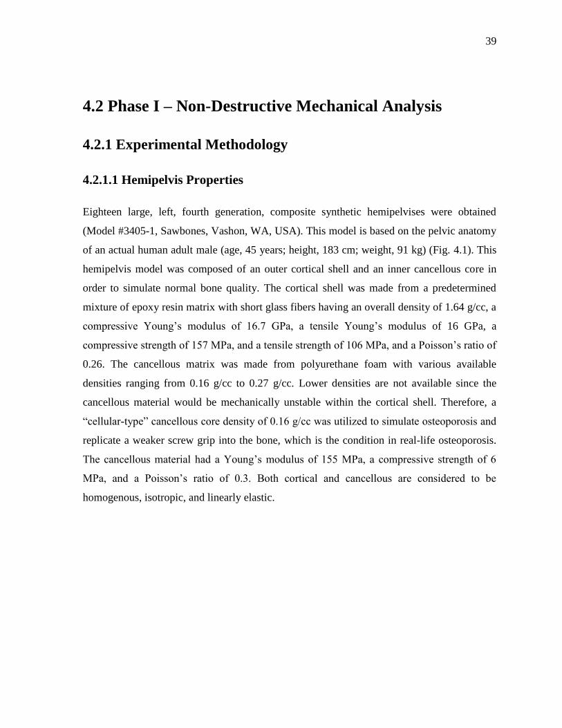
39

4.2 Phase I – Non-Destructive Mechanical Analysis

4.2.1 Experimental Methodology

4.2.1.1 Hemipelvis Properties

Eighteen large, left, fourth generation, composite synthetic hemipelvises were obtained

(Model #3405-1, Sawbones, Vashon, WA, USA). This model is based on the pelvic anatomy

of an actual human adult male (age, 45 years; height, 183 cm; weight, 91 kg) (Fig. 4.1). This

hemipelvis model was composed of an outer cortical shell and an inner cancellous core in

order to simulate normal bone quality. The cortical shell was made from a predetermined

mixture of epoxy resin matrix with short glass fibers having an overall density of 1.64 g/cc, a

compressive Young’s modulus of 16.7 GPa, a tensile Young’s modulus of 16 GPa, a

compressive strength of 157 MPa, and a tensile strength of 106 MPa, and a Poisson’s ratio of

0.26. The cancellous matrix was made from polyurethane foam with various available

densities ranging from 0.16 g/cc to 0.27 g/cc. Lower densities are not available since the

cancellous material would be mechanically unstable within the cortical shell. Therefore, a

“cellular-type” cancellous core density of 0.16 g/cc was utilized to simulate osteoporosis and

replicate a weaker screw grip into the bone, which is the condition in real-life osteoporosis.

The cancellous material had a Young’s modulus of 155 MPa, a compressive strength of 6

MPa, and a Poisson’s ratio of 0.3. Both cortical and cancellous are considered to be

homogenous, isotropic, and linearly elastic.

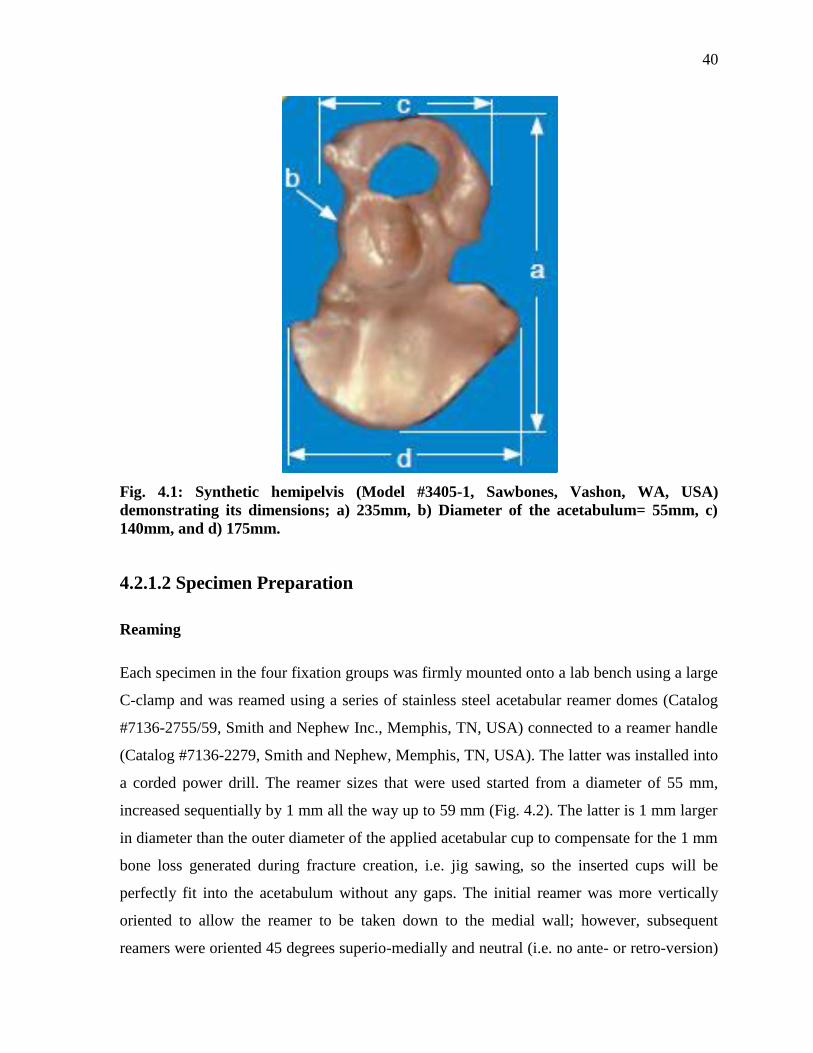
40

Fig. 4.1: Synthetic hemipelvis (Model #3405-1, Sawbones, Vashon, WA, USA)

demonstrating its dimensions; a) 235mm, b) Diameter of the acetabulum= 55mm, c)

140mm, and d) 175mm.

4.2.1.2 Specimen Preparation

Reaming

Each specimen in the four fixation groups was firmly mounted onto a lab bench using a large

C-clamp and was reamed using a series of stainless steel acetabular reamer domes (Catalog

#7136-2755/59, Smith and Nephew Inc., Memphis, TN, USA) connected to a reamer handle

(Catalog #7136-2279, Smith and Nephew, Memphis, TN, USA). The latter was installed into

a corded power drill. The reamer sizes that were used started from a diameter of 55 mm,

increased sequentially by 1 mm all the way up to 59 mm (Fig. 4.2). The latter is 1 mm larger

in diameter than the outer diameter of the applied acetabular cup to compensate for the 1 mm

bone loss generated during fracture creation, i.e. jig sawing, so the inserted cups will be

perfectly fit into the acetabulum without any gaps. The initial reamer was more vertically

oriented to allow the reamer to be taken down to the medial wall; however, subsequent

reamers were oriented 45 degrees superio-medially and neutral (i.e. no ante- or retro-version)

41

in the sagittal plane, which is the standard surgical practice for reaming and final acetabular

cup alignment. Excess medialization of the cup was avoided to preserve the thin medial wall,

and hence, provide good support to the acetabular shell. Reaming was the first step

performed in because it would be impossible to precisely ream the hard cortical shell and

cancellous core after creating the complex AHT fracture.

Fracture Creation

Each specimen that was firmly mounted using a C-clamp onto a lab bench was then had a

simulated fracture created using a 120V, 1-1/8” corded reciprocating jigsaw (Model #RS7,

Bosch, Home Depot, Canada). An anterior fracture was created first extending superiorly

from ½ inch (12.7 mm) anterior to the gluteal line on the iliac crest, cutting the acetabular

ring in the anterior third until reaching the Obturator Foramen, and exiting inferiorly close to

the junction between the Inferior Pubic Ramus and Inferior Ischial Ramus. The posterior

portion of the hemipelvis was then flipped so that the cut surface faced the lab bench and an

oblique hemitransverse fracture was created being high medially at the tip of the Greater

Sciatic Notch and low laterally at the dome of the acetabulum, thus making an angle of 40

degrees with the transverse plane. Anteriorly, the hemitransverse fracture met with the

anterior fracture just above the Arcuate Line of the Ilium, creating a small triangular area

with that line, which represents the typical clinical pattern of the AHT associated acetabular

fractures (Fig. 4.2).

Fracture Reduction

Each specimen was divided into 3 fragments after creating the AHT fracture: an anterior

fragment, a posterior-superior fragment, and a posterior-inferior fragment. To fix the fracture

with the different methods, these 3 pieces needed to be anatomically reduced first. A

reduction clamp and four 2.5 mm K-wires were used. To reduce the anterior fracture, the

reduction clamp was installed first and connected two holes in the cortex across the fracture.

The first hole was provided by the manufacturer at the base of the anterior inferior iliac spine

(AIIS), while another superficial hole was created in the cortex 1.5” (38 mm) above the

superior rim of the acetabulum using a 2.7 mm drill bit. These two holes allowed the

reduction clamp to firmly grip the two fragments across the fracture. In addition, two parallel

42

K-wires were inserted across the anterior fracture at two different levels above the reduction

clamp. For the reduction of the transverse fracture, other two K-wires were inserted

divergently across the fracture line at two different levels (Fig. 4.2). All the reduction tools

were kept in place until the specimen was accurately fixed and the acetabular component

with the liner was inserted. This order of events would replicate the typical surgical

technique and achieve the best possible reduction, and hence, biomechanical stability for

each of the four different fixation methods.

Cup Insertion

After creating the fracture, reducing and fixing it, an acetabular component of a THA was

inserted (Fig. 4.3) to simulate the clinical situation of the simultaneous fixation of complex

associated acetabular fractures and performing a THA at the same setting in elderly patients

with osteoporosis, osteopenia, impaction or comminution of the acetabulum or femoral head.

The fixation is performed first in a trial to provide good support for the acetabular cup and

minimize medial and superior displacement. For this purpose, a size G with an outer diameter

of 58mm, multi-hole acetabular shell (Reflection, Model# 71335158, Smith and Nephew

Inc., Memphis, TN, USA) was installed. The shell was made of titanium alloy (Ti-6Al-4V),

which would provide reasonable stiffness and at the same time is light in weight. The outer

surface of the shell was porous to stimulate bone growth and entanglement of bone fibers and

cells around these small pores at a micro-level leading to better mechanical stability. The

acetabular shell was connected to a straight acetabular shell impactor (R3 straight shell

impactor, catalog# 7136-4450, Smith and Nephew Inc., Memphis, TN, USA) and an X-Bar

(Catalog# MT-2201, Smith and Nephew Inc., Memphis, TN, USA) was mounted on top to

allow proper alignment of the cup with 45 degrees of abduction and neutral version of the

cup. A mallet (Reflection mallet, Catalog# 7136-2106, Smith and Nephew Inc., Memphis,

TN, USA) was used to tap on the impactor for proper insertion of the shell providing good

contact with the medial wall of the acetabulum. The X-Bar was removed and the impactor

was then unscrewed from the shell. Four pilot holes were drilled using a 3.5mm, 50mm long

flexible screw drill (Catalog# 7136-2950, Smith and Nephew Inc., Memphis, TN, USA). The

orientation of the pilot holes and screws exactly matched the real-life surgical practice. A

depth gauge was used to measure the depth of the holes for choosing the right length screws.

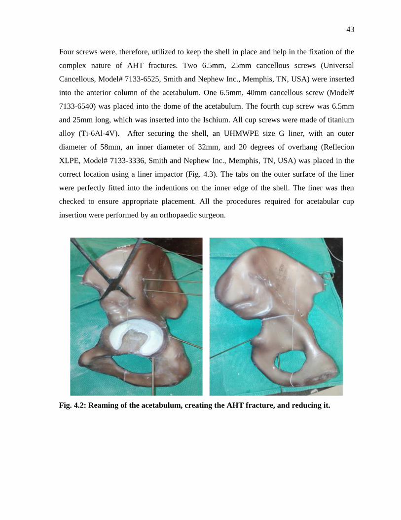
43

Four screws were, therefore, utilized to keep the shell in place and help in the fixation of the

complex nature of AHT fractures. Two 6.5mm, 25mm cancellous screws (Universal

Cancellous, Model# 7133-6525, Smith and Nephew Inc., Memphis, TN, USA) were inserted

into the anterior column of the acetabulum. One 6.5mm, 40mm cancellous screw (Model#

7133-6540) was placed into the dome of the acetabulum. The fourth cup screw was 6.5mm

and 25mm long, which was inserted into the Ischium. All cup screws were made of titanium

alloy (Ti-6Al-4V). After securing the shell, an UHMWPE size G liner, with an outer

diameter of 58mm, an inner diameter of 32mm, and 20 degrees of overhang (Reflecion

XLPE, Model# 7133-3336, Smith and Nephew Inc., Memphis, TN, USA) was placed in the

correct location using a liner impactor (Fig. 4.3). The tabs on the outer surface of the liner

were perfectly fitted into the indentions on the inner edge of the shell. The liner was then

checked to ensure appropriate placement. All the procedures required for acetabular cup

insertion were performed by an orthopaedic surgeon.

Fig. 4.2: Reaming of the acetabulum, creating the AHT fracture, and reducing it.

44

Fig. 4.3: Left: acetabular shell insertion. Right: acetabular liner insertion.

Fracture Groups

Intact: The “Intact” hemipelvis group. specimens were not fractured nor repaired and acted

as a baseline or control group.

Cup: The “Cup” group was composed of intact hemipelvises equipped with an acetabular

metal cup and polyethylene liner, in order to detect the influence of a THR’s acetabular

component on the stiffness and stress distribution.

Plate: The “Plate” group was composed of hemipelvises with an AHT acetabular fracture

repaired with a posterior column plate and anterior column lag screw (Fig. 4.4). This is

considered the “gold standard” of care applied for complex acetabular fractures and is the

most commonly used technique performed by the majority of orthopaedic surgeons

specializing in trauma and pelvic fractures (Knight and Smith, 1958; Letournel and Judet,

1993; Levine, 1943; Matta, 1996). For each specimen of the plate group, a 3.5, 6-hole, 70mm

long stainless steel reconstruction plate (Model# 71809516, Peri-Loc, Smith and Nephew

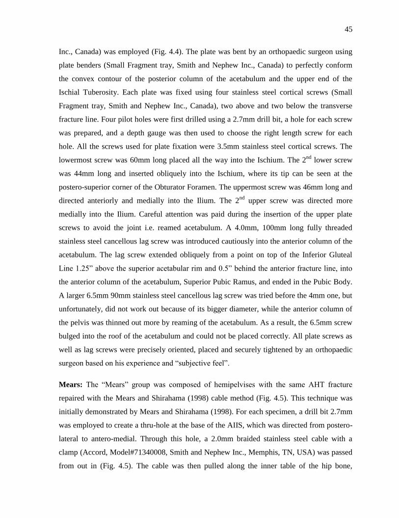
45

Inc., Canada) was employed (Fig. 4.4). The plate was bent by an orthopaedic surgeon using

plate benders (Small Fragment tray, Smith and Nephew Inc., Canada) to perfectly conform

the convex contour of the posterior column of the acetabulum and the upper end of the

Ischial Tuberosity. Each plate was fixed using four stainless steel cortical screws (Small

Fragment tray, Smith and Nephew Inc., Canada), two above and two below the transverse

fracture line. Four pilot holes were first drilled using a 2.7mm drill bit, a hole for each screw

was prepared, and a depth gauge was then used to choose the right length screw for each

hole. All the screws used for plate fixation were 3.5mm stainless steel cortical screws. The

lowermost screw was 60mm long placed all the way into the Ischium. The 2nd

lower screw

was 44mm long and inserted obliquely into the Ischium, where its tip can be seen at the

postero-superior corner of the Obturator Foramen. The uppermost screw was 46mm long and

directed anteriorly and medially into the Ilium. The 2nd

upper screw was directed more

medially into the Ilium. Careful attention was paid during the insertion of the upper plate

screws to avoid the joint i.e. reamed acetabulum. A 4.0mm, 100mm long fully threaded

stainless steel cancellous lag screw was introduced cautiously into the anterior column of the

acetabulum. The lag screw extended obliquely from a point on top of the Inferior Gluteal

Line 1.25” above the superior acetabular rim and 0.5” behind the anterior fracture line, into

the anterior column of the acetabulum, Superior Pubic Ramus, and ended in the Pubic Body.

A larger 6.5mm 90mm stainless steel cancellous lag screw was tried before the 4mm one, but

unfortunately, did not work out because of its bigger diameter, while the anterior column of

the pelvis was thinned out more by reaming of the acetabulum. As a result, the 6.5mm screw

bulged into the roof of the acetabulum and could not be placed correctly. All plate screws as

well as lag screws were precisely oriented, placed and securely tightened by an orthopaedic

surgeon based on his experience and “subjective feel”.

Mears: The “Mears” group was composed of hemipelvises with the same AHT fracture

repaired with the Mears and Shirahama (1998) cable method (Fig. 4.5). This technique was

initially demonstrated by Mears and Shirahama (1998). For each specimen, a drill bit 2.7mm

was employed to create a thru-hole at the base of the AIIS, which was directed from postero-

lateral to antero-medial. Through this hole, a 2.0mm braided stainless steel cable with a

clamp (Accord, Model#71340008, Smith and Nephew Inc., Memphis, TN, USA) was passed

from out in (Fig. 4.5). The cable was then pulled along the inner table of the hip bone,

46

crossing the point of meeting of both fractures and the Arcuate Line of the Ilium, proceeding

along the quadrilateral plate of the acetabulum to the Lesser Sciatic Notch (LSN), where it

curves around from medial to lateral. The cable then crosses the lateral surface of the Ischium

to the postero-superior end of the Obturator foramen, where it curves medially again, going

up along the quadrilateral plate, where it makes a cross sign with the previous path of the

cable on the inner side of the hip bone, till it reaches the Greater Sciatic Notch (GSN). At the

GSN, it changes path again from in out, where it continues anteriorly to meet the beginning

of the cable above the superior rim of the acetabulum. The end of the cable was then run

through the clamp at the head of the cable creating a loop. The cable was then held in place

till the free end of the cable was passed through the tip of the Accord cable tensioner

(Catalog# 7136-0020, Smith and Nephew Inc., Memphis, TN, USA). Before using the

tensioner, the “Reset Switch” was turned clockwise to reset the tensioner, while the “Locking

Handle” was open. The free end of the cable was then passed all the way in through the

tensioner until the tensioner was in direct contact with the clamp with no gaps. The “Locking

Handle” was then turned clockwise to hold the cable firmly and prevent any slippage of the

cable under tension. The “Lever” on the tensioner was then pumped until the “Tension

Gauge” reached 100Kg. The clamp was checked to ensure that the cable ran through it

properly and the clamp screw was strongly tightened until clicking sound was heard using a

fitting surgical screwdriver. The cable was then loosened from the tensioner by turning the

“Locking Handle” counterclockwise and the tensioner was removed.

Kang: The “Kang” group was composed of hemipelvises with the same AHT fracture

repaired with the Kang and Min (2002) cable method (Fig. 4.6). Two 2.0mm braided

stainless steel cables (Accord, Model#71340008, Smith and Nephew Inc., Memphis, TN,

USA) were used for this fixation method (Fig. 4.6), as originally discussed by Kang and Min

(2002). The first cable was wrapped around the hip bone from just above the AIIS, turning

around the anterior border of the bone from lateral to medial, then going posteriorly on the

inner table of the Ilium crossing the Arcuate line to the GSN, where it curves around it from

in out running on the outer surface of the Ilium, until it passed through the clamp forming a

full loop. The clamp rested on the Iliac bone about 1” above the superior rim of the

acetabulum. Then, the same tensioning technique was applied as described above in the

“Mears fixation” section. This cable mainly provided fixation across the anterior fracture

47

component of the AHT fracture pattern. The other cable was also run just above the base of

the AIIS, going around the anterior border of the hemipelvis from lateral to medial, but this

time the cable was passed posteriorly and inferiorly on the medial side of the pelvis, crossing

the Iliac Fossa, the arcuate line, and across the anterior fracture. The cable was then passed

across the quadrilateral plate providing support to this important region necessary for the

success of fixation, and turned around the LSN to meet the other end and pass through the

clamp about 0.5” above the superior acetabular rim. The same tensioning technique was

employed as discussed in “Mears fixation” section. This cable provided compression across

both components of the AHT associated acetabular fracture as well as supported the

quadrilateral plate of the acetabulum.

Mouhsine: The “Mouhsine” group was composed of hemipelvises with the same AHT

fracture repaired with the Mouhsine et al. (2002) cable method (Fig. 4.7). This method

required just one 2.0mm braided stainless steel cable (Accord, Model#71340008, Smith and

Nephew Inc., Memphis, TN, USA) as originally described by Mouhsine et al. (2002) (Fig.

4.7). In this fixation method, the cable was passed posteriorly and inferiorly above the

superior acetabular rim towards the LSN, where the cable turns around it going up through

another clamp held on the quadrilateral plate, then curved down again to pass through the

postero-superior end of the obturator foramen. The cable was then directed posteriorly and

superiorly in the Groove for the Obturator Externus tendon until it reached the GSN, where it

curved down on the quadrilateral plate again to run through the clamp held there and exit

from its anterior end, crossing the rest of the quadrilateral plate, arcuate line until it reached a

point just above the AIIS, where it turned around to run through the clamp at the beginning

of the cable forming a closed loop. The exact same tensioning procedure was used for this

cable as the one mentioned in “Mears Fixation” section. This cable provided reasonable

fixation to both components of the complex AHT acetabular fracture as well as good support

to the quadrilateral plate in a trial to prevent medialization of the acetabular cup under the

influence of force generated during daily life activities.

48

Fig. 4.4: The “Plate” fixation method. A posterior column plate with an anterior

column lag screw. Left: lateral view. Right: medial view. An acetabular cup was

inserted.

Fig. 4.5: The “Mears” fixation method. A 2.0 mm braided cable with clamp was

employed. Left: lateral view. Right: medial view. An acetabular cup was inserted.

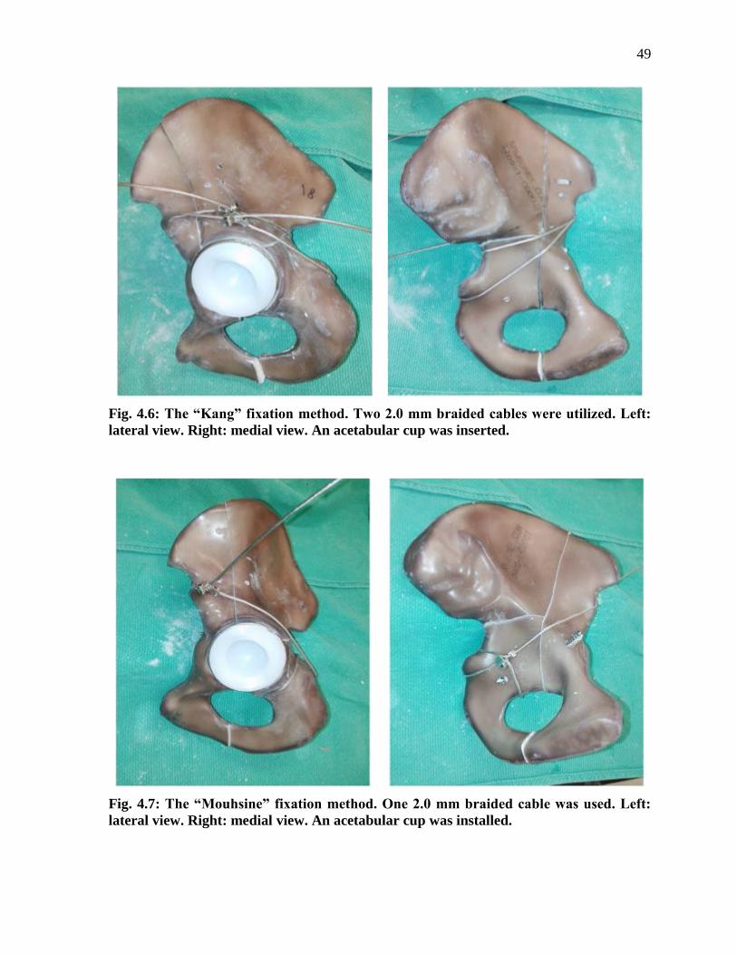
49

Fig. 4.6: The “Kang” fixation method. Two 2.0 mm braided cables were utilized. Left:

lateral view. Right: medial view. An acetabular cup was inserted.

Fig. 4.7: The “Mouhsine” fixation method. One 2.0 mm braided cable was used. Left:

lateral view. Right: medial view. An acetabular cup was installed.

50

4.2.1.3 Mechanical Test Jig

For the proper fixation and alignment of the specimens, a unique setup was designed and

manufactured. The setup provided proper anatomical orientation of the acetabulum during

femoral head force application during normal daily physiological activities. The setup also

provided anatomical fixation of the hemipelvis at the Sacro-iliac (SI) and Symphysis Pubis

(SP) regions as would occur physiologically. To this end, two hollow steel cubes (3.46" wide

X 3.46” long X 2.95” high) were employed. Two thru-holes were drilled at specific locations

to bolt the cubes together at 30 degree angle to one another. One of the surfaces of the top

cube provided a good support to the pelvis at the SI area by using three #10, 2” fully threaded

stainless steel socket head cup screws with washers and fixed in place by one nut at the end

of each screw. A steel block (1.25” long X 1” wide X 9” high) was manufactured and

connected to one side of the bottom cube by two threaded screws into threaded holes. This

side block had four threaded holes on top, where it supported the SP region by the use of 1¼”

fully threaded stainless steel socket head cup screw (Fig. 4.8 and 4.9). The setup was rigidly

mounted on a vise (4” wide X 1½” deep jaws) with an adjustable angle ranging from 0 to 90

degrees. The setup allowed anatomical orientation of the acetabulum, where both the ASIS

and the front of the top of the SP were aligned in the same coronal plane producing a force

vector of 45 degrees superomedially and 20 degrees posteriorly with the mechanical tester in

the sagittal plane, which approximates the position of the femoral head in the standing

position (Bergmann et al., 1993; Chang et al., 2001; Khajavi et al., 2010; Letournel and

Judet, 1993; Shazar et al., 1998; Witte et al., 1997). To mount each specimen, four holes

were drilled: one at the SP area using an 11/64” drill bit for a ¼” metal screw, and three at

the SI region in a supero-inferior line using a 9/64 inch drill bit for #10 metal screws. Drilling

the right holes for mounting each specimen on the setup was done after reaming, fracturing,

reducing, and repairing the hemipelvises to prevent pre-stressing the bone or the repair

constructs. To simulate the femoral component of a THR for a size G acetabular cup and

liner, an aluminum alloy ball was used which had an outer diameter of 1.26” and a short neck

(0.59” diameter X 0.39” long). The metal ball was mounted to the mechanical tester and load

cell using a stainless steel rod (1” diameter X 3” length). The lower surface of the rod had an

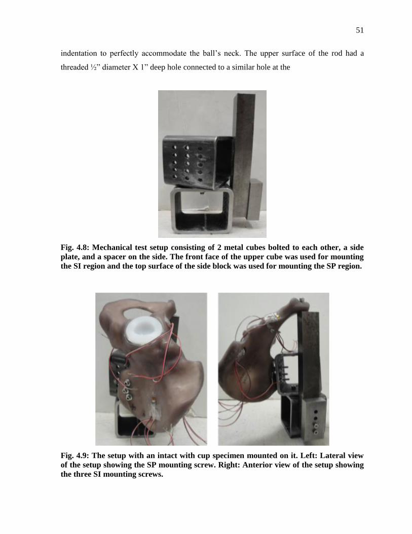
51

indentation to perfectly accommodate the ball’s neck. The upper surface of the rod had a

threaded ½” diameter X 1” deep hole connected to a similar hole at the

Fig. 4.8: Mechanical test setup consisting of 2 metal cubes bolted to each other, a side

plate, and a spacer on the side. The front face of the upper cube was used for mounting

the SI region and the top surface of the side block was used for mounting the SP region.

Fig. 4.9: The setup with an intact with cup specimen mounted on it. Left: Lateral view

of the setup showing the SP mounting screw. Right: Anterior view of the setup showing

the three SI mounting screws.

52

centre of an aluminum alloy rectangular plate (5.51” long X 3.54” wide X 0.5” thick) with a

½” diameter X 1¼” long stainless steel set screws. The plate was then attached to the load

cell of the mechanical tester using four bolts.

4.2.1.4 Strain Gauges

Gauge Specifications

To accommodate the complex 3D specimen geometry, rosette strain gauges (Model# CEA-

06-062UR-350, Vishay Measurements Group, Raleigh, NC, USA) were selected to be the

most suitable (Vishay Measurements Group, 2010). These rosettes have an overall grid

resistance of 350.0 Ω ±0.4%. Each rosette has 3 grids at 45° angles in respect to each other so

that it would detect strains on the surface of an object in 2 perpendicular directions and at 45°

in between (Fig. 4.10). Each grip has a certain gauge factor (GF) provided by the

manufacturer, which was used later for accurate calculation of strains. The GF for grid 1, 2,

and 3, respectively, were 2.085 ± 0.5%, 2.105 ± 0.5%, and 2.085 ± 0.5%, with an overall GF

for all three grids of 2.10 ± 1.5%.

Gauge Locations

Gauges were physically mounted according to the manufacturer’s instructions to ensure

consistent and accurate readings (Vishay Measurements Group, 2011). Anatomical markers

were used as references for consistent gauge placement. Locations were chosen based on

geometry and to cover all the three bone fragments, medial and lateral surfaces of the

hemipelvis, above and below the transverse fracture line, and on either side of the anterior

fracture line. For the Intact group, five rosettes were instrumented on each specimen at the

following five locations, while for the other five groups, only four rosettes were used at

locations 1-4 (Fig. 4.11).

Location 1: The lower left corner of the rosette gauge was mounted on the outer surface of

the Ilium, at a distance of 87 mm from the ASIS and 86 mm from the PIIS. For all four

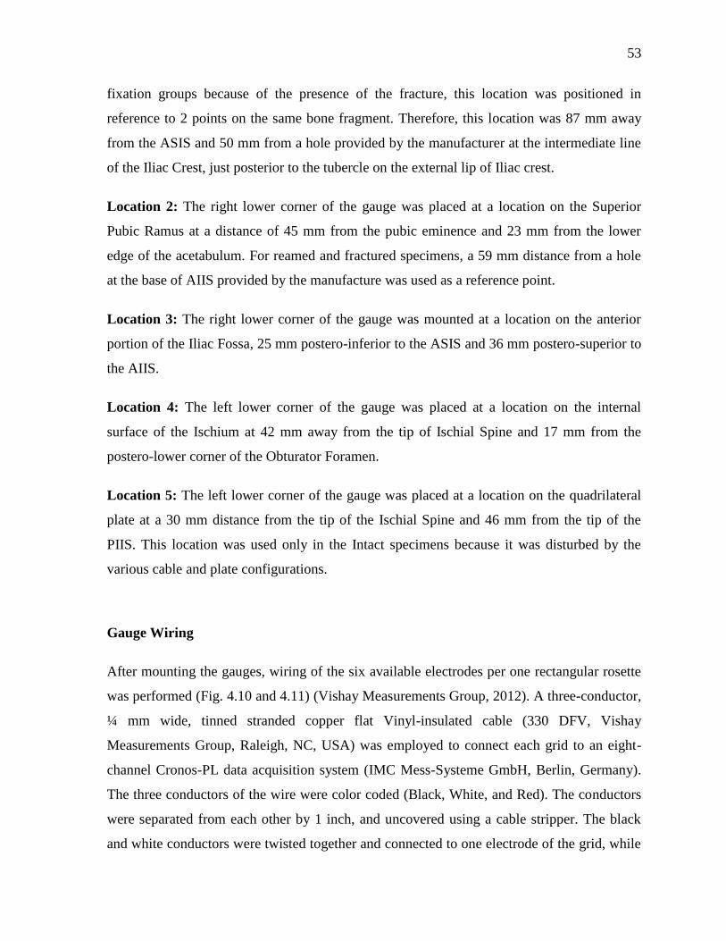
53

fixation groups because of the presence of the fracture, this location was positioned in

reference to 2 points on the same bone fragment. Therefore, this location was 87 mm away

from the ASIS and 50 mm from a hole provided by the manufacturer at the intermediate line

of the Iliac Crest, just posterior to the tubercle on the external lip of Iliac crest.

Location 2: The right lower corner of the gauge was placed at a location on the Superior

Pubic Ramus at a distance of 45 mm from the pubic eminence and 23 mm from the lower

edge of the acetabulum. For reamed and fractured specimens, a 59 mm distance from a hole

at the base of AIIS provided by the manufacture was used as a reference point.

Location 3: The right lower corner of the gauge was mounted at a location on the anterior

portion of the Iliac Fossa, 25 mm postero-inferior to the ASIS and 36 mm postero-superior to

the AIIS.

Location 4: The left lower corner of the gauge was placed at a location on the internal

surface of the Ischium at 42 mm away from the tip of Ischial Spine and 17 mm from the

postero-lower corner of the Obturator Foramen.

Location 5: The left lower corner of the gauge was placed at a location on the quadrilateral

plate at a 30 mm distance from the tip of the Ischial Spine and 46 mm from the tip of the

PIIS. This location was used only in the Intact specimens because it was disturbed by the

various cable and plate configurations.

Gauge Wiring

After mounting the gauges, wiring of the six available electrodes per one rectangular rosette

was performed (Fig. 4.10 and 4.11) (Vishay Measurements Group, 2012). A three-conductor,

¼ mm wide, tinned stranded copper flat Vinyl-insulated cable (330 DFV, Vishay

Measurements Group, Raleigh, NC, USA) was employed to connect each grid to an eight-

channel Cronos-PL data acquisition system (IMC Mess-Systeme GmbH, Berlin, Germany).

The three conductors of the wire were color coded (Black, White, and Red). The conductors

were separated from each other by 1 inch, and uncovered using a cable stripper. The black

and white conductors were twisted together and connected to one electrode of the grid, while

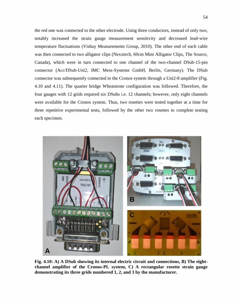
54

the red one was connected to the other electrode. Using three conductors, instead of only two,

notably increased the strain gauge measurement sensitivity and decreased lead-wire

temperature fluctuations (Vishay Measurements Group, 2010). The other end of each cable

was then connected to two alligator clips (Nexxtech, 60cm Mini Alligator Clips, The Source,

Canada), which were in turn connected to one channel of the two-channel DSub-15-pin

connector (Acc/DSub-Uni2, IMC Mess-Systeme GmbH, Berlin, Germany). The DSub

connector was subsequently connected to the Cronos system through a Uni2-8 amplifier (Fig.

4.10 and 4.11). The quarter bridge Wheatstone configuration was followed. Therefore, the

four gauges with 12 grids required six DSubs i.e. 12 channels; however, only eight channels

were available for the Cronos system. Thus, two rosettes were tested together at a time for

three repetitive experimental tests, followed by the other two rosettes to complete testing

each specimen.

Fig. 4.10: A) A DSub showing its internal electric circuit and connections, B) The eight-

channel amplifier of the Cronos-PL system, C) A rectangular rosette strain gauge

demonstrating its three grids numbered 1, 2, and 3 by the manufacturer.

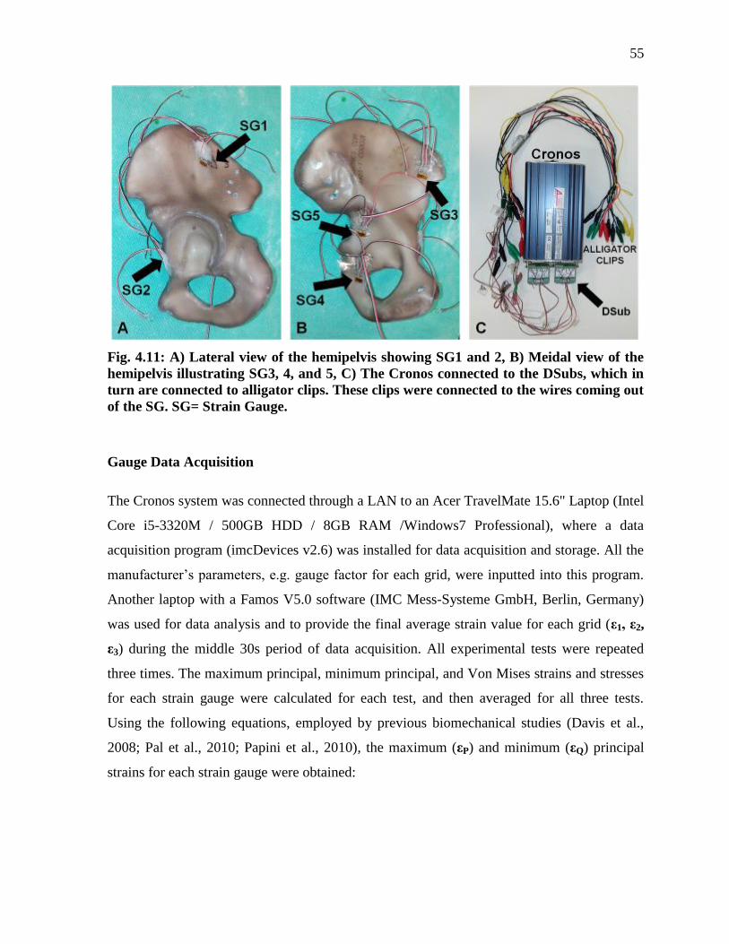
55

Fig. 4.11: A) Lateral view of the hemipelvis showing SG1 and 2, B) Meidal view of the

hemipelvis illustrating SG3, 4, and 5, C) The Cronos connected to the DSubs, which in

turn are connected to alligator clips. These clips were connected to the wires coming out

of the SG. SG= Strain Gauge.

Gauge Data Acquisition

The Cronos system was connected through a LAN to an Acer TravelMate 15.6" Laptop (Intel

Core i5-3320M / 500GB HDD / 8GB RAM /Windows7 Professional), where a data

acquisition program (imcDevices v2.6) was installed for data acquisition and storage. All the

manufacturer’s parameters, e.g. gauge factor for each grid, were inputted into this program.

Another laptop with a Famos V5.0 software (IMC Mess-Systeme GmbH, Berlin, Germany)

was used for data analysis and to provide the final average strain value for each grid (ε1, ε2,

ε3) during the middle 30s period of data acquisition. All experimental tests were repeated

three times. The maximum principal, minimum principal, and Von Mises strains and stresses

for each strain gauge were calculated for each test, and then averaged for all three tests.

Using the following equations, employed by previous biomechanical studies (Davis et al.,

2008; Pal et al., 2010; Papini et al., 2010), the maximum (εP) and minimum (εQ) principal

strains for each strain gauge were obtained:

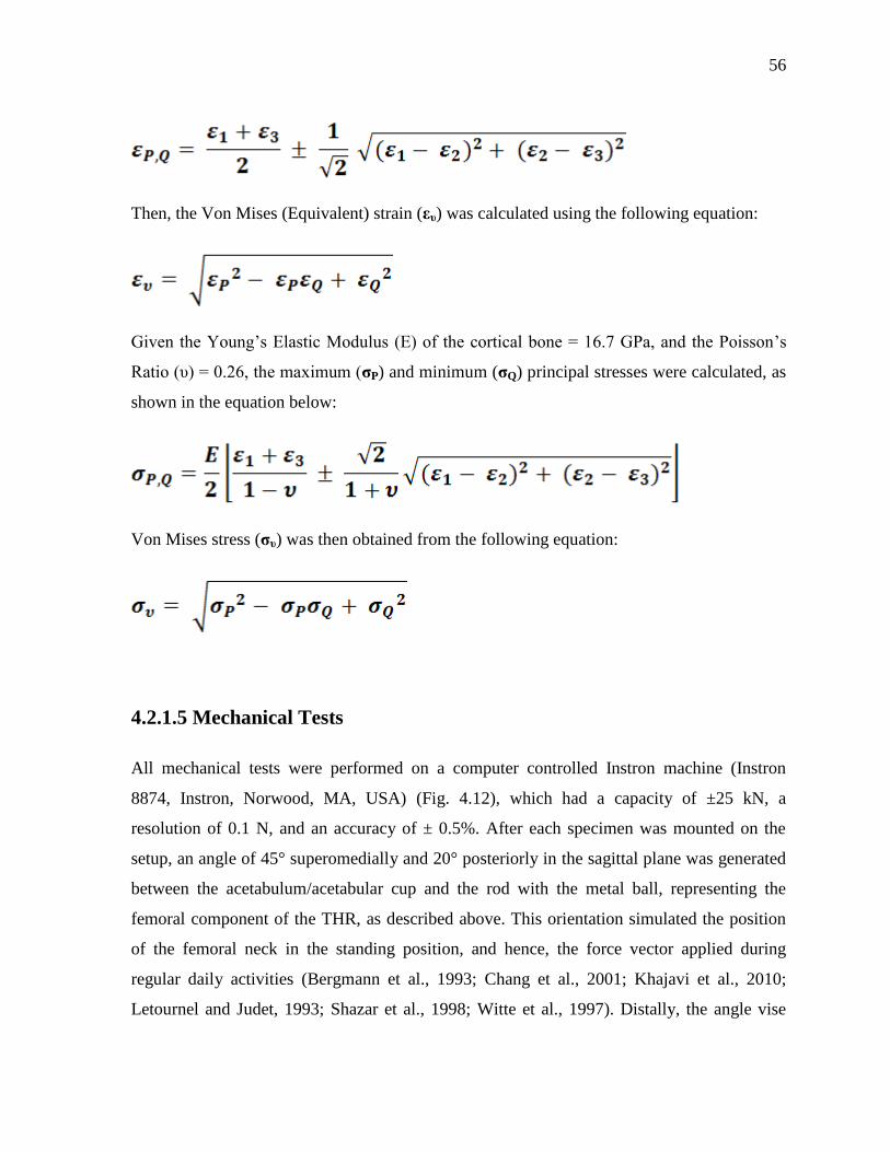
56

Then, the Von Mises (Equivalent) strain (ευ) was calculated using the following equation:

Given the Young’s Elastic Modulus (E) of the cortical bone = 16.7 GPa, and the Poisson’s

Ratio (υ) = 0.26, the maximum (σP) and minimum (σQ) principal stresses were calculated, as

shown in the equation below:

Von Mises stress (συ) was then obtained from the following equation:

4.2.1.5 Mechanical Tests

All mechanical tests were performed on a computer controlled Instron machine (Instron

8874, Instron, Norwood, MA, USA) (Fig. 4.12), which had a capacity of ±25 kN, a

resolution of 0.1 N, and an accuracy of ± 0.5%. After each specimen was mounted on the

setup, an angle of 45° superomedially and 20° posteriorly in the sagittal plane was generated

between the acetabulum/acetabular cup and the rod with the metal ball, representing the

femoral component of the THR, as described above. This orientation simulated the position

of the femoral neck in the standing position, and hence, the force vector applied during

regular daily activities (Bergmann et al., 1993; Chang et al., 2001; Khajavi et al., 2010;

Letournel and Judet, 1993; Shazar et al., 1998; Witte et al., 1997). Distally, the angle vise

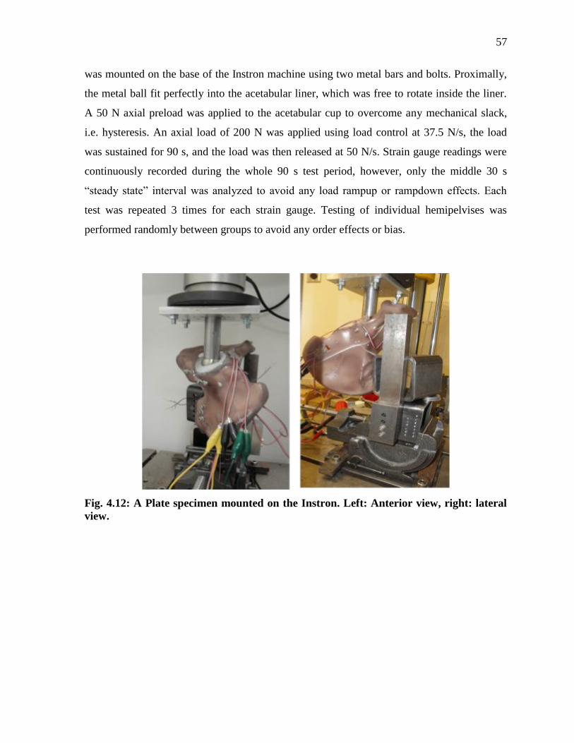
57

was mounted on the base of the Instron machine using two metal bars and bolts. Proximally,

the metal ball fit perfectly into the acetabular liner, which was free to rotate inside the liner.

A 50 N axial preload was applied to the acetabular cup to overcome any mechanical slack,

i.e. hysteresis. An axial load of 200 N was applied using load control at 37.5 N/s, the load

was sustained for 90 s, and the load was then released at 50 N/s. Strain gauge readings were

continuously recorded during the whole 90 s test period, however, only the middle 30 s

“steady state” interval was analyzed to avoid any load rampup or rampdown effects. Each

test was repeated 3 times for each strain gauge. Testing of individual hemipelvises was

performed randomly between groups to avoid any order effects or bias.

Fig. 4.12: A Plate specimen mounted on the Instron. Left: Anterior view, right: lateral

view.

58

4.2.2 Finite Element Analysis (FEA)

4.2.2.1 CAD Models

Hemipelvis

The 3D CAD files in SolidWorks format (SolidWorks Corp., Dassault Systèmes, Concord,

MA, USA) for the same left, large, fourth generation, composite hemipelvis described earlier

were supplied by the manufacturer (Model #3405, Sawbones, Vashon, WA, USA) (Fig.

4.13). The geometry consisted of two bodies, i.e. a solid cortex and a solid cancellous core,

which was oriented in the anatomical position. Each body consisted of a certain number of

faces. Before any processing, the cortex and cancellous core were originally made of 581 and

294 faces, respectively.

Implants

The femoral metal ball, side block, steel cube, and fixation screws for the setup were

designed using SolidWorks 2014 x 64 software based on measurements of the physical setup

obtained using a digital caliper with a resolution of 0.01 mm. The size G multi-hole

acetabular shell and polyethylene liner (Smith and Nephew Inc., Memphis, TN, USA) were

modeled according to the parameters provided by the manufacturer plus digital caliper

measurements. Plates were designed to conform to the complex surface of the posterior

column of the hemipelvis with dimension obtained using the digital caliper. Employing the

“Spline” and “3 point Arc” features in SolidWorks, the curved plate was sketched to simulate

the exact plate course. Then, using the “Sweep” function, the plate was generated and refined

using the “Extruded Cut”, “Fillet”, and “Curve Driven Pattern” functions. Also, all cup

screws, plate screws, and lag screws were designed according to manufacturer specifications

plus digital caliper measurements for the diameters and shapes of screw heads. All screw

threads were neglected because a previous study showed no significant difference for

threaded vs. non-threaded screws if the contact at the bone/screw interface is assigned a

“Bonded” contact, as done currently (Zdero et al., 2008a). For cables, a 3D drawing was

59

utilized to allow the precise replication of the path of the cable. Many points were added on

the cortex along the cable’s path, then the “Spline” utility was used to connect these points

together, creating a closed loop that simulated the exact orientation of the cable. The

“Sweep” utility was then employed to create the 3D cable body. The points along the path

were occasionally used to refine the orientation of the cable.

4.2.2.2 Component Assembly

For each of the six FE groups, the relevant parts were assembled using SolidWorks 2014 x

64 Edition Assembly (SolidWorks Corp., Dassault Systèmes, Concord, MA, USA).

For the Intact group (Fig. 4.14), the four fixation screws at the SI and SP regions were passed

through cortical and cancellous bodies with the same orientation used for the experimental

setup. The steel cube and side block were placed and oriented properly with respect to the

pelvis, thereby touching the cortex to support the bone in the SI and SP areas, as done

experimentally. The femoral metal ball was placed in contact with the acetabulum. A

pressure-sensitive Fujifilm was inserted between the ball and the acetabulum to determine the

exact shape and size of the contact area. The ball was oriented at 45° superomedially and 20°

posteriorly in the sagittal plane to simulate the anatomical position of the femoral neck in the

standing position, and therefore, apply physiological loads along the correct force vector

yielded in human hips during routine daily activities.

For the Cup group (Fig. 4.14), a hemi-spherical body with a diameter of 59 mm was

introduced into the acetabulum to simulate the largest size of the used reamers. Another 59

mm circular body was introduced on top of the hemispherical body to overlap with any

protruding bone along the acetabular rim. Also, the acetabular shell and liner were put in

place in relation to the acetabulum. Four cup screws were inserted: two in the anterior

column, one in the posterior column, and the last one in the Ischium, replicating the correct

surgical placement of these screws. The model was eventually shown to an orthopaedic

surgeon for approval.

60

Finally, the four fixation groups (Fig. 4.15 and 4.16) were then assembled based on the Cup

group with the addition of the corresponding fixation implants.

4.2.2.3 Assembly Processing

The six previous assemblies for the six FE models were saved as “STEP AP214” files, which

were imported and read by the latest version of ANSYS Workbech R15.0 DesignModeler

(ANSYS Inc., Canonsburg, PA, USA). The latter was used for further processing of the six

assembly models as follows:

For the Intact group (Fig. 4.14), because the rectangular sketches resembling strain gauges

were projected onto the cortex, each drawing did not form a separate entity. Therefore, the

“Merge” function was used to merge the involved faces together forming that rectangular

new face with the exact same location and size as experimental strain gauges. This task was

performed for each of the strain gauges for each of the six models. Also, necessary Boolean

operations were performed between the assembled bodies such as between the cortex and

core on one hand and the fixation screws and femoral ball on the other hand.

For the Cup groups (Fig. 4.14), the previous tasks were performed along with the “Delete –

Body” function, which was used to delete the hemispherical and circular bodies used to

simulate reaming of the acetabulum.

For the four fixation groups (Fig. 4.15 and 4.16), the above functions were used, plus planes

were created along which the “Slice” feature was utilized to create the AHT fracture. This

fracture pattern typically matched the one created in experimental specimens.

4.2.2.4 Boundary Conditions

For the Intact model, the fixation screws at both SI and SP regions were “bonded” with no

slipping at all cortical/cancellous bones, steel cube, and side block because screws were

tightly threaded through the bone and nuts were used at the SI region, while threaded into the

side block. The contact between the side block and steel cube to the cortex was assigned to

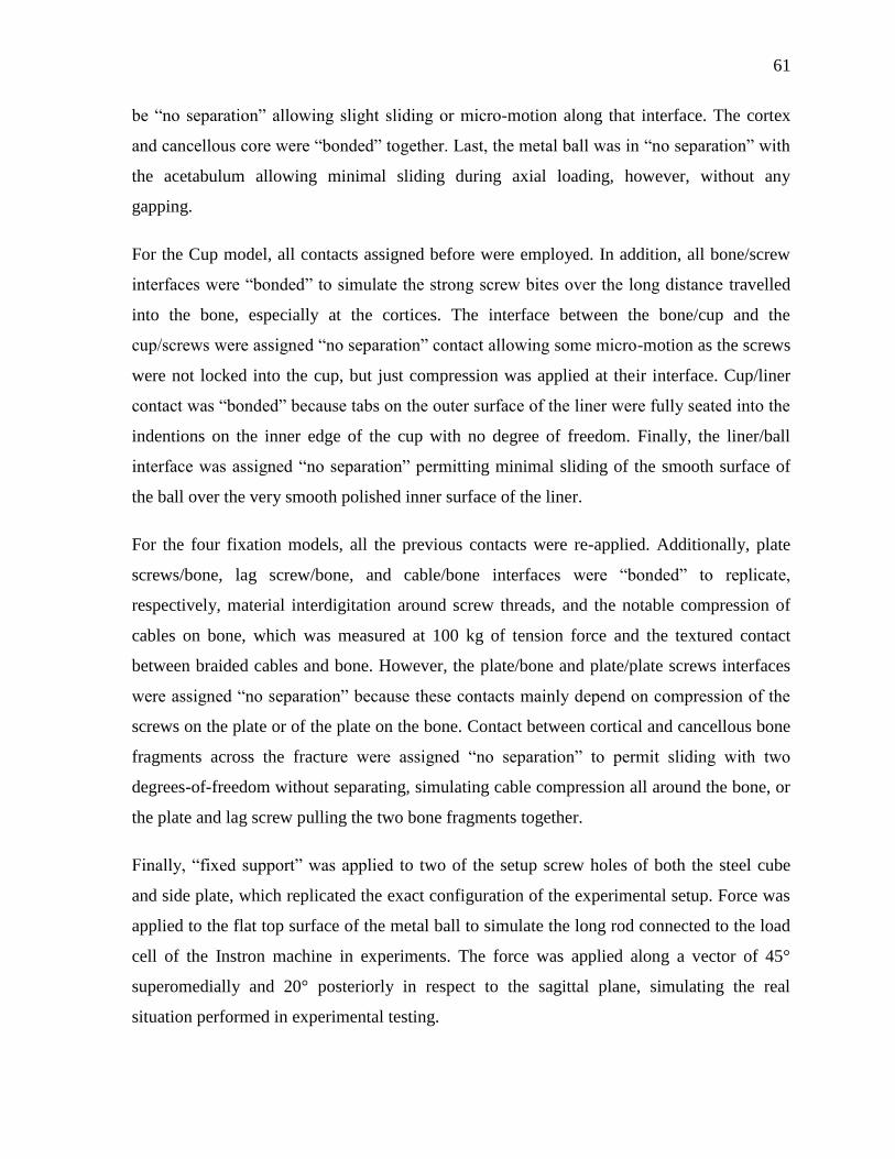
61

be “no separation” allowing slight sliding or micro-motion along that interface. The cortex

and cancellous core were “bonded” together. Last, the metal ball was in “no separation” with

the acetabulum allowing minimal sliding during axial loading, however, without any

gapping.

For the Cup model, all contacts assigned before were employed. In addition, all bone/screw

interfaces were “bonded” to simulate the strong screw bites over the long distance travelled

into the bone, especially at the cortices. The interface between the bone/cup and the

cup/screws were assigned “no separation” contact allowing some micro-motion as the screws

were not locked into the cup, but just compression was applied at their interface. Cup/liner

contact was “bonded” because tabs on the outer surface of the liner were fully seated into the

indentions on the inner edge of the cup with no degree of freedom. Finally, the liner/ball

interface was assigned “no separation” permitting minimal sliding of the smooth surface of

the ball over the very smooth polished inner surface of the liner.

For the four fixation models, all the previous contacts were re-applied. Additionally, plate

screws/bone, lag screw/bone, and cable/bone interfaces were “bonded” to replicate,

respectively, material interdigitation around screw threads, and the notable compression of

cables on bone, which was measured at 100 kg of tension force and the textured contact

between braided cables and bone. However, the plate/bone and plate/plate screws interfaces

were assigned “no separation” because these contacts mainly depend on compression of the

screws on the plate or of the plate on the bone. Contact between cortical and cancellous bone

fragments across the fracture were assigned “no separation” to permit sliding with two

degrees-of-freedom without separating, simulating cable compression all around the bone, or

the plate and lag screw pulling the two bone fragments together.

Finally, “fixed support” was applied to two of the setup screw holes of both the steel cube

and side plate, which replicated the exact configuration of the experimental setup. Force was

applied to the flat top surface of the metal ball to simulate the long rod connected to the load

cell of the Instron machine in experiments. The force was applied along a vector of 45°

superomedially and 20° posteriorly in respect to the sagittal plane, simulating the real

situation performed in experimental testing.

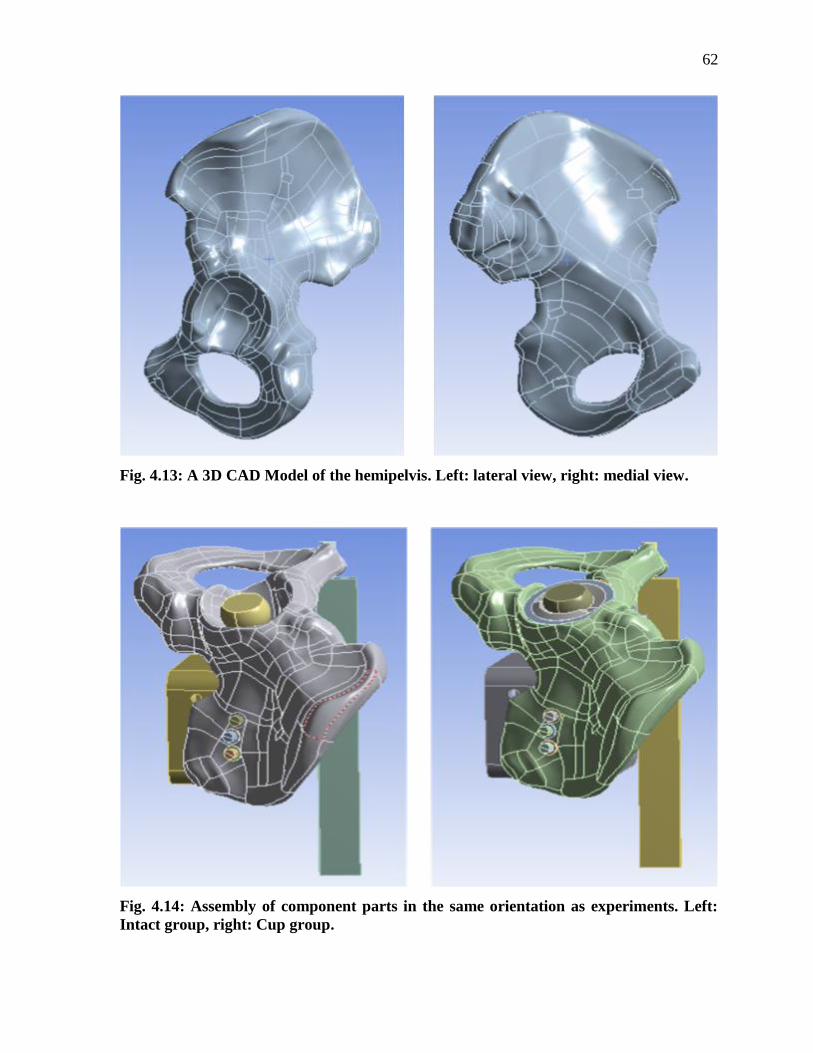
62

Fig. 4.13: A 3D CAD Model of the hemipelvis. Left: lateral view, right: medial view.

Fig. 4.14: Assembly of component parts in the same orientation as experiments. Left:

Intact group, right: Cup group.

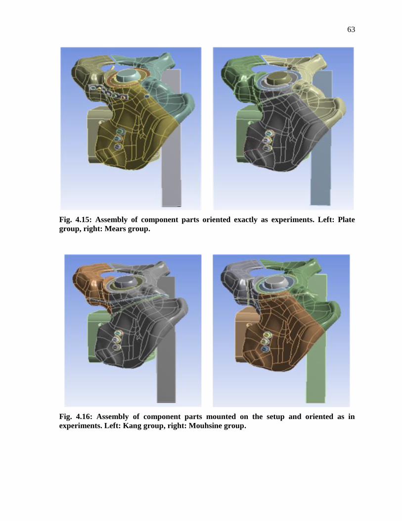
63

Fig. 4.15: Assembly of component parts oriented exactly as experiments. Left: Plate

group, right: Mears group.

Fig. 4.16: Assembly of component parts mounted on the setup and oriented as in

experiments. Left: Kang group, right: Mouhsine group.

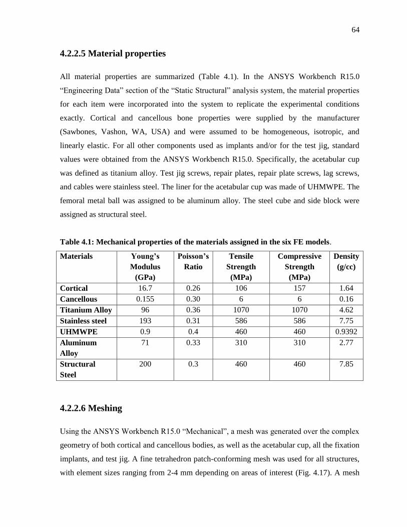
64

4.2.2.5 Material properties

All material properties are summarized (Table 4.1). In the ANSYS Workbench R15.0

“Engineering Data” section of the “Static Structural” analysis system, the material properties

for each item were incorporated into the system to replicate the experimental conditions

exactly. Cortical and cancellous bone properties were supplied by the manufacturer

(Sawbones, Vashon, WA, USA) and were assumed to be homogeneous, isotropic, and

linearly elastic. For all other components used as implants and/or for the test jig, standard

values were obtained from the ANSYS Workbench R15.0. Specifically, the acetabular cup

was defined as titanium alloy. Test jig screws, repair plates, repair plate screws, lag screws,

and cables were stainless steel. The liner for the acetabular cup was made of UHMWPE. The

femoral metal ball was assigned to be aluminum alloy. The steel cube and side block were

assigned as structural steel.

Table 4.1: Mechanical properties of the materials assigned in the six FE models.

Materials Young’s

Modulus

(GPa)

Poisson’s

Ratio

Tensile

Strength

(MPa)

Compressive

Strength

(MPa)

Density

(g/cc)

Cortical 16.7 0.26 106 157 1.64

Cancellous 0.155 0.30 6 6 0.16

Titanium Alloy 96 0.36 1070 1070 4.62

Stainless steel 193 0.31 586 586 7.75

UHMWPE 0.9 0.4 460 460 0.9392

Aluminum

Alloy

71 0.33 310 310 2.77

Structural

Steel

200 0.3 460 460 7.85

4.2.2.6 Meshing

Using the ANSYS Workbench R15.0 “Mechanical”, a mesh was generated over the complex

geometry of both cortical and cancellous bodies, as well as the acetabular cup, all the fixation

implants, and test jig. A fine tetrahedron patch-conforming mesh was used for all structures,

with element sizes ranging from 2-4 mm depending on areas of interest (Fig. 4.17). A mesh

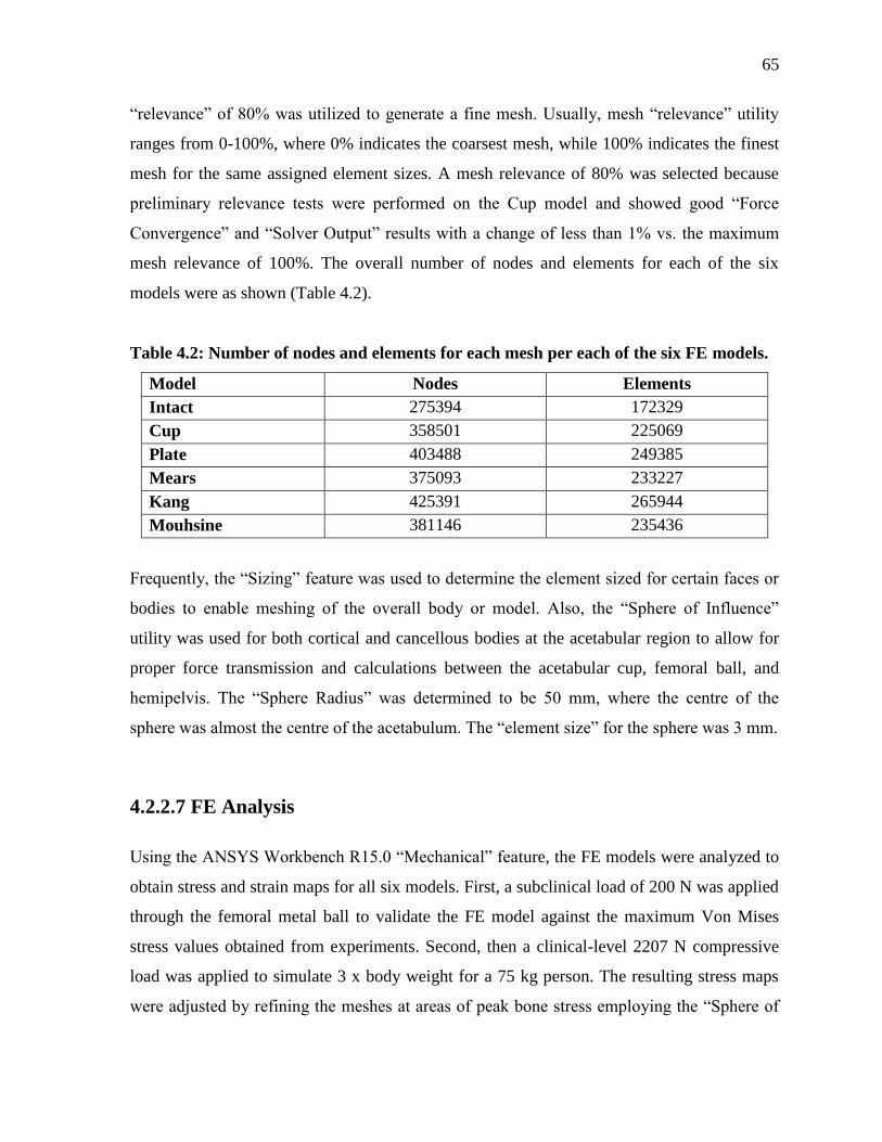
65

“relevance” of 80% was utilized to generate a fine mesh. Usually, mesh “relevance” utility

ranges from 0-100%, where 0% indicates the coarsest mesh, while 100% indicates the finest

mesh for the same assigned element sizes. A mesh relevance of 80% was selected because

preliminary relevance tests were performed on the Cup model and showed good “Force

Convergence” and “Solver Output” results with a change of less than 1% vs. the maximum

mesh relevance of 100%. The overall number of nodes and elements for each of the six

models were as shown (Table 4.2).

Table 4.2: Number of nodes and elements for each mesh per each of the six FE models.

Model Nodes Elements

Intact 275394 172329

Cup 358501 225069

Plate 403488 249385

Mears 375093 233227

Kang 425391 265944

Mouhsine 381146 235436

Frequently, the “Sizing” feature was used to determine the element sized for certain faces or

bodies to enable meshing of the overall body or model. Also, the “Sphere of Influence”

utility was used for both cortical and cancellous bodies at the acetabular region to allow for

proper force transmission and calculations between the acetabular cup, femoral ball, and

hemipelvis. The “Sphere Radius” was determined to be 50 mm, where the centre of the

sphere was almost the centre of the acetabulum. The “element size” for the sphere was 3 mm.

4.2.2.7 FE Analysis

Using the ANSYS Workbench R15.0 “Mechanical” feature, the FE models were analyzed to

obtain stress and strain maps for all six models. First, a subclinical load of 200 N was applied

through the femoral metal ball to validate the FE model against the maximum Von Mises

stress values obtained from experiments. Second, then a clinical-level 2207 N compressive

load was applied to simulate 3 x body weight for a 75 kg person. The resulting stress maps

were adjusted by refining the meshes at areas of peak bone stress employing the “Sphere of

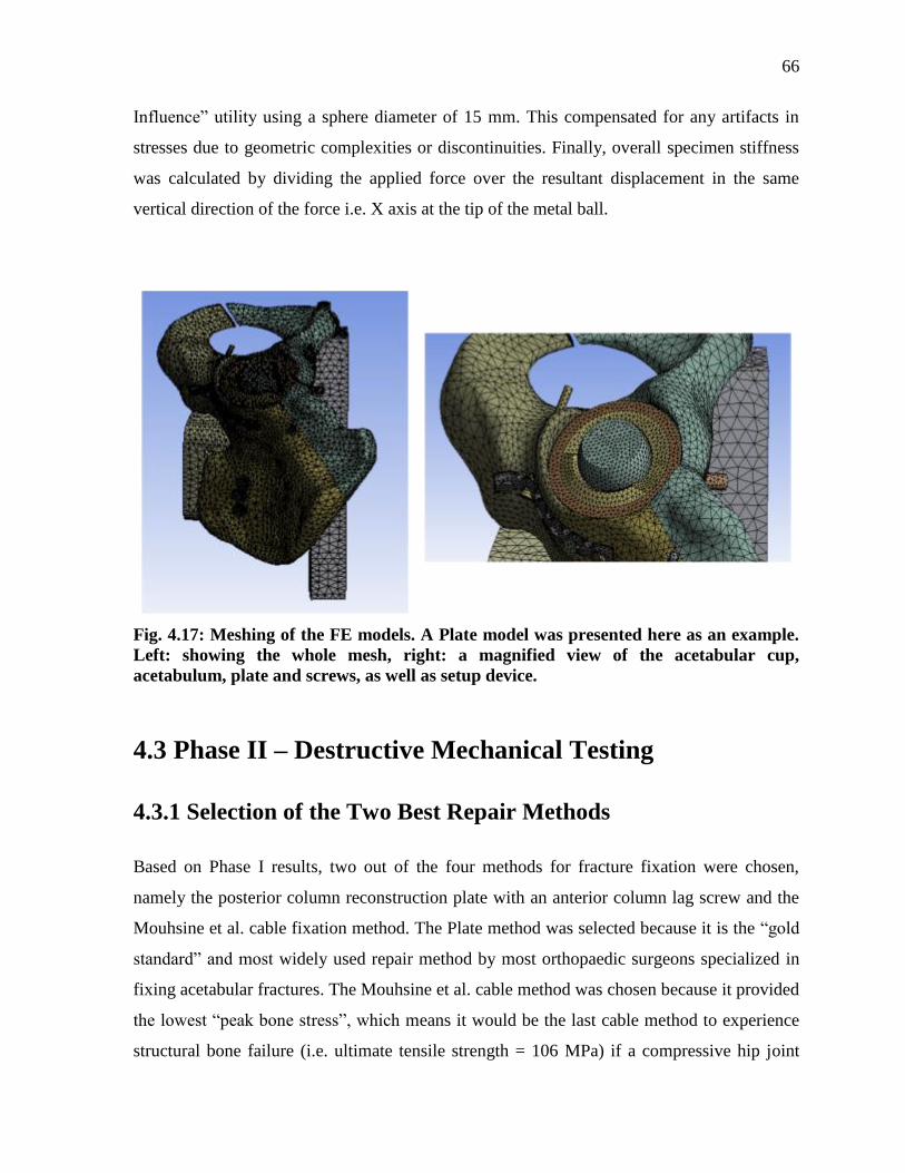
66

Influence” utility using a sphere diameter of 15 mm. This compensated for any artifacts in

stresses due to geometric complexities or discontinuities. Finally, overall specimen stiffness

was calculated by dividing the applied force over the resultant displacement in the same

vertical direction of the force i.e. X axis at the tip of the metal ball.

Fig. 4.17: Meshing of the FE models. A Plate model was presented here as an example.

Left: showing the whole mesh, right: a magnified view of the acetabular cup,

acetabulum, plate and screws, as well as setup device.

4.3 Phase II – Destructive Mechanical Testing

4.3.1 Selection of the Two Best Repair Methods

Based on Phase I results, two out of the four methods for fracture fixation were chosen,

namely the posterior column reconstruction plate with an anterior column lag screw and the

Mouhsine et al. cable fixation method. The Plate method was selected because it is the “gold

standard” and most widely used repair method by most orthopaedic surgeons specialized in

fixing acetabular fractures. The Mouhsine et al. cable method was chosen because it provided

the lowest “peak bone stress”, which means it would be the last cable method to experience

structural bone failure (i.e. ultimate tensile strength = 106 MPa) if a compressive hip joint

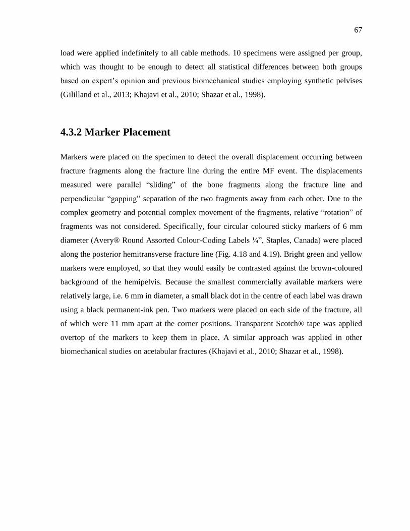
67

load were applied indefinitely to all cable methods. 10 specimens were assigned per group,

which was thought to be enough to detect all statistical differences between both groups

based on expert’s opinion and previous biomechanical studies employing synthetic pelvises

(Gililland et al., 2013; Khajavi et al., 2010; Shazar et al., 1998).

4.3.2 Marker Placement

Markers were placed on the specimen to detect the overall displacement occurring between

fracture fragments along the fracture line during the entire MF event. The displacements

measured were parallel “sliding” of the bone fragments along the fracture line and

perpendicular “gapping” separation of the two fragments away from each other. Due to the

complex geometry and potential complex movement of the fragments, relative “rotation” of

fragments was not considered. Specifically, four circular coloured sticky markers of 6 mm

diameter (Avery® Round Assorted Colour-Coding Labels ¼”, Staples, Canada) were placed

along the posterior hemitransverse fracture line (Fig. 4.18 and 4.19). Bright green and yellow

markers were employed, so that they would easily be contrasted against the brown-coloured

background of the hemipelvis. Because the smallest commercially available markers were

relatively large, i.e. 6 mm in diameter, a small black dot in the centre of each label was drawn

using a black permanent-ink pen. Two markers were placed on each side of the fracture, all

of which were 11 mm apart at the corner positions. Transparent Scotch® tape was applied

overtop of the markers to keep them in place. A similar approach was applied in other

biomechanical studies on acetabular fractures (Khajavi et al., 2010; Shazar et al., 1998).

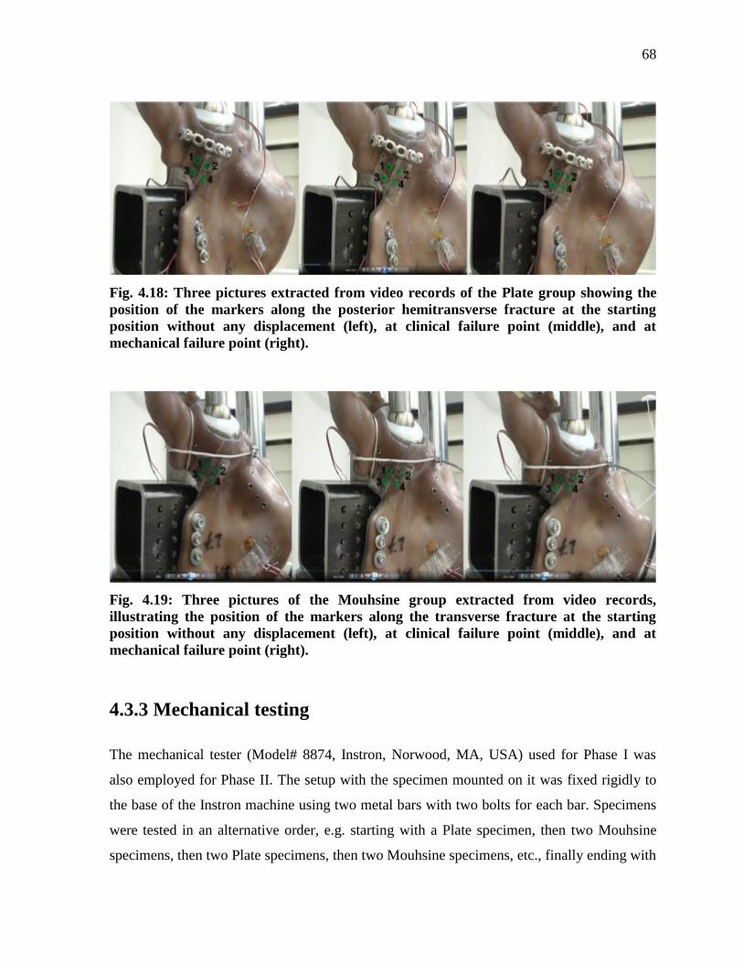
68

Fig. 4.18: Three pictures extracted from video records of the Plate group showing the

position of the markers along the posterior hemitransverse fracture at the starting

position without any displacement (left), at clinical failure point (middle), and at

mechanical failure point (right).

Fig. 4.19: Three pictures of the Mouhsine group extracted from video records,

illustrating the position of the markers along the transverse fracture at the starting

position without any displacement (left), at clinical failure point (middle), and at

mechanical failure point (right).

4.3.3 Mechanical testing

The mechanical tester (Model# 8874, Instron, Norwood, MA, USA) used for Phase I was

also employed for Phase II. The setup with the specimen mounted on it was fixed rigidly to

the base of the Instron machine using two metal bars with two bolts for each bar. Specimens

were tested in an alternative order, e.g. starting with a Plate specimen, then two Mouhsine

specimens, then two Plate specimens, then two Mouhsine specimens, etc., finally ending with

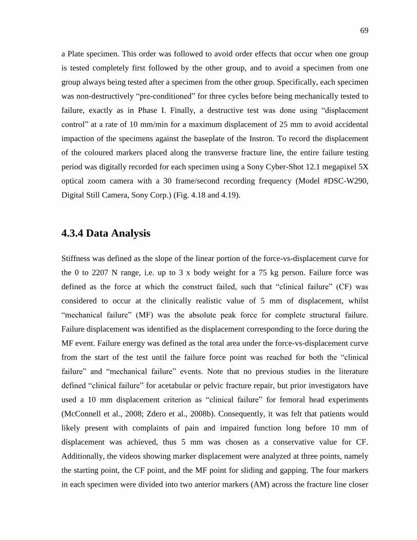
69

a Plate specimen. This order was followed to avoid order effects that occur when one group

is tested completely first followed by the other group, and to avoid a specimen from one

group always being tested after a specimen from the other group. Specifically, each specimen

was non-destructively “pre-conditioned” for three cycles before being mechanically tested to

failure, exactly as in Phase I. Finally, a destructive test was done using “displacement

control” at a rate of 10 mm/min for a maximum displacement of 25 mm to avoid accidental

impaction of the specimens against the baseplate of the Instron. To record the displacement

of the coloured markers placed along the transverse fracture line, the entire failure testing

period was digitally recorded for each specimen using a Sony Cyber-Shot 12.1 megapixel 5X

optical zoom camera with a 30 frame/second recording frequency (Model #DSC-W290,

Digital Still Camera, Sony Corp.) (Fig. 4.18 and 4.19).

4.3.4 Data Analysis

Stiffness was defined as the slope of the linear portion of the force-vs-displacement curve for

the 0 to 2207 N range, i.e. up to 3 x body weight for a 75 kg person. Failure force was

defined as the force at which the construct failed, such that “clinical failure” (CF) was

considered to occur at the clinically realistic value of 5 mm of displacement, whilst

“mechanical failure” (MF) was the absolute peak force for complete structural failure.

Failure displacement was identified as the displacement corresponding to the force during the

MF event. Failure energy was defined as the total area under the force-vs-displacement curve

from the start of the test until the failure force point was reached for both the “clinical

failure” and “mechanical failure” events. Note that no previous studies in the literature

defined “clinical failure” for acetabular or pelvic fracture repair, but prior investigators have

used a 10 mm displacement criterion as “clinical failure” for femoral head experiments

(McConnell et al., 2008; Zdero et al., 2008b). Consequently, it was felt that patients would

likely present with complaints of pain and impaired function long before 10 mm of

displacement was achieved, thus 5 mm was chosen as a conservative value for CF.

Additionally, the videos showing marker displacement were analyzed at three points, namely

the starting point, the CF point, and the MF point for sliding and gapping. The four markers

in each specimen were divided into two anterior markers (AM) across the fracture line closer

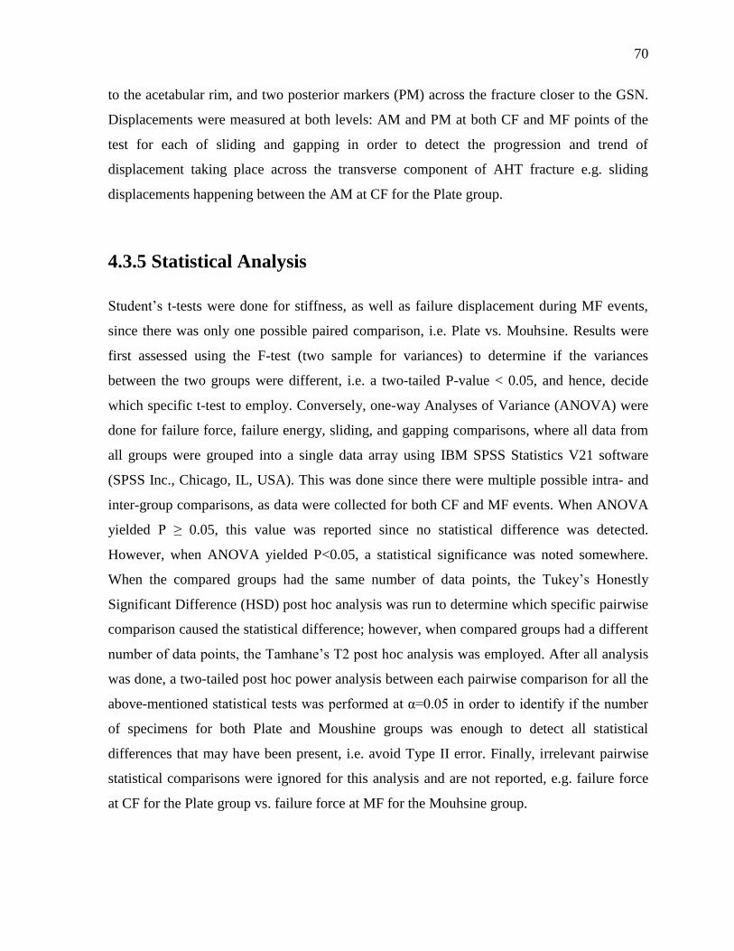
70

to the acetabular rim, and two posterior markers (PM) across the fracture closer to the GSN.

Displacements were measured at both levels: AM and PM at both CF and MF points of the

test for each of sliding and gapping in order to detect the progression and trend of

displacement taking place across the transverse component of AHT fracture e.g. sliding

displacements happening between the AM at CF for the Plate group.

4.3.5 Statistical Analysis

Student’s t-tests were done for stiffness, as well as failure displacement during MF events,

since there was only one possible paired comparison, i.e. Plate vs. Mouhsine. Results were

first assessed using the F-test (two sample for variances) to determine if the variances

between the two groups were different, i.e. a two-tailed P-value < 0.05, and hence, decide

which specific t-test to employ. Conversely, one-way Analyses of Variance (ANOVA) were

done for failure force, failure energy, sliding, and gapping comparisons, where all data from

all groups were grouped into a single data array using IBM SPSS Statistics V21 software

(SPSS Inc., Chicago, IL, USA). This was done since there were multiple possible intra- and

inter-group comparisons, as data were collected for both CF and MF events. When ANOVA

yielded P ≥ 0.05, this value was reported since no statistical difference was detected.

However, when ANOVA yielded P<0.05, a statistical significance was noted somewhere.

When the compared groups had the same number of data points, the Tukey’s Honestly

Significant Difference (HSD) post hoc analysis was run to determine which specific pairwise

comparison caused the statistical difference; however, when compared groups had a different

number of data points, the Tamhane’s T2 post hoc analysis was employed. After all analysis

was done, a two-tailed post hoc power analysis between each pairwise comparison for all the

above-mentioned statistical tests was performed at α=0.05 in order to identify if the number

of specimens for both Plate and Moushine groups was enough to detect all statistical

differences that may have been present, i.e. avoid Type II error. Finally, irrelevant pairwise

statistical comparisons were ignored for this analysis and are not reported, e.g. failure force

at CF for the Plate group vs. failure force at MF for the Mouhsine group.

71

Chapter 5

Results

5.1 Phase I: Non-Destructive Analysis of Hemipelvises

5.1.1 Experimental Validation of FEA

For the non-destructive experiments at 200 N, results of the overall average experimental

results for each strain gauge per each group are summarized (Table 5.1). The corresponding

FEA results for Von Mises stress values are also provided (Table 5.2).

Table 5.1: Experimental Von Mises Stress Values in MPa. SG = strain gauge.

Strain Gauge Intact Cup Plate Mears Kang Mouhsine

SG1 0.279 0.250 0.333 0.179 0.243 0.374

SG2 1.738 0.826 2.942 0.857 1.503 0.931

SG3 0.291 0.441 0.197 0.385 0.415 0.361

SG4 0.451 0.284 0.129 0.205 0.159 0.411

SG5 0.953

Table 5.2: FEA Von Mises Stress Values in MPa at each Strain Gauge Location. SG =

strain gage.

Strain Gauge

Location

Intact Cup Plate Mears Kang Mouhsine

SG1 0.151 0.211 0.296 0.308 0.231 0.306

SG2 1.154 1.321 1.306 1.527 1.437 1.439

SG3 0.110 0.109 0.032 0.079 0.059 0.078

SG4 0.519 0.288 0.069 0.081 0.066 0.054

SG5 0.437

All data points for Von Mises stress obtained from experiments and FEA were plotted

against each other to detect the correlation, since they FE models are essentially variations of

one and the same model (Fig. 5.1). This approach was adopted by many biomechanical

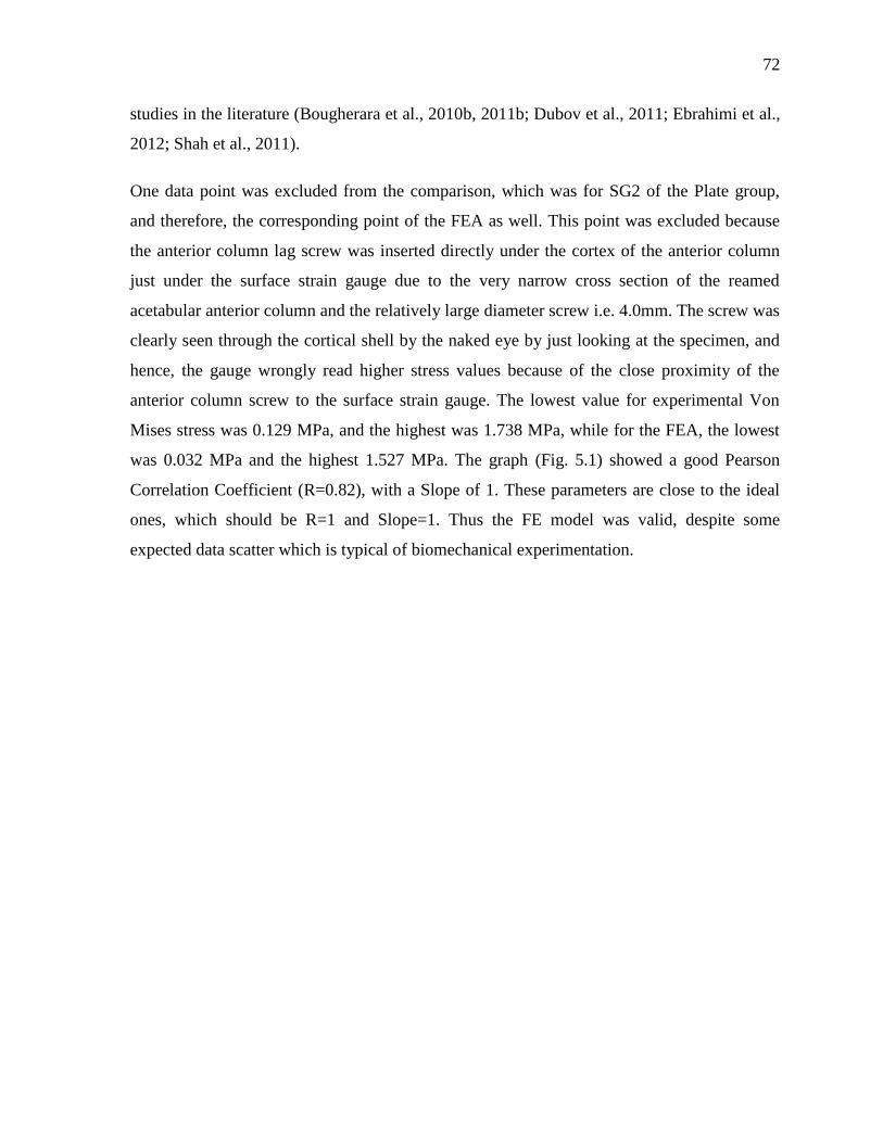
72

studies in the literature (Bougherara et al., 2010b, 2011b; Dubov et al., 2011; Ebrahimi et al.,

2012; Shah et al., 2011).

One data point was excluded from the comparison, which was for SG2 of the Plate group,

and therefore, the corresponding point of the FEA as well. This point was excluded because

the anterior column lag screw was inserted directly under the cortex of the anterior column

just under the surface strain gauge due to the very narrow cross section of the reamed

acetabular anterior column and the relatively large diameter screw i.e. 4.0mm. The screw was

clearly seen through the cortical shell by the naked eye by just looking at the specimen, and

hence, the gauge wrongly read higher stress values because of the close proximity of the

anterior column screw to the surface strain gauge. The lowest value for experimental Von

Mises stress was 0.129 MPa, and the highest was 1.738 MPa, while for the FEA, the lowest

was 0.032 MPa and the highest 1.527 MPa. The graph (Fig. 5.1) showed a good Pearson

Correlation Coefficient (R=0.82), with a Slope of 1. These parameters are close to the ideal

ones, which should be R=1 and Slope=1. Thus the FE model was valid, despite some

expected data scatter which is typical of biomechanical experimentation.

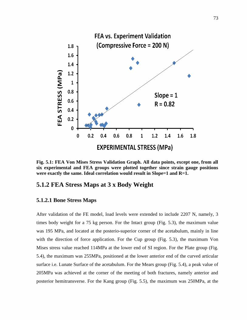
73

Fig. 5.1: FEA Von Mises Stress Validation Graph. All data points, except one, from all

six experimental and FEA groups were plotted together since strain gauge positions

were exactly the same. Ideal correlation would result in Slope=1 and R=1.

5.1.2 FEA Stress Maps at 3 x Body Weight

5.1.2.1 Bone Stress Maps

After validation of the FE model, load levels were extended to include 2207 N, namely, 3

times body weight for a 75 kg person. For the Intact group (Fig. 5.3), the maximum value

was 195 MPa, and located at the posterio-superior corner of the acetabulum, mainly in line

with the direction of force application. For the Cup group (Fig. 5.3), the maximum Von

Mises stress value reached 114MPa at the lower end of SI region. For the Plate group (Fig.

5.4), the maximum was 255MPa, positioned at the lower anterior end of the curved articular

surface i.e. Lunate Surface of the acetabulum. For the Mears group (Fig. 5.4), a peak value of

205MPa was achieved at the corner of the meeting of both fractures, namely anterior and

posterior hemitransverse. For the Kang group (Fig. 5.5), the maximum was 250MPa, at the

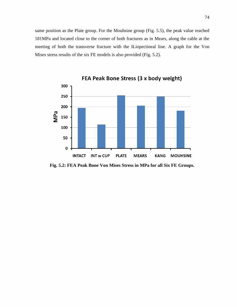
74

same position as the Plate group. For the Mouhsine group (Fig. 5.5), the peak value reached

181MPa and located close to the corner of both fractures as in Mears, along the cable at the

meeting of both the transverse fracture with the ILiopectineal line. A graph for the Von

Mises stress results of the six FE models is also provided (Fig. 5.2).

Fig. 5.2: FEA Peak Bone Von Mises Stress in MPa for all Six FE Groups.

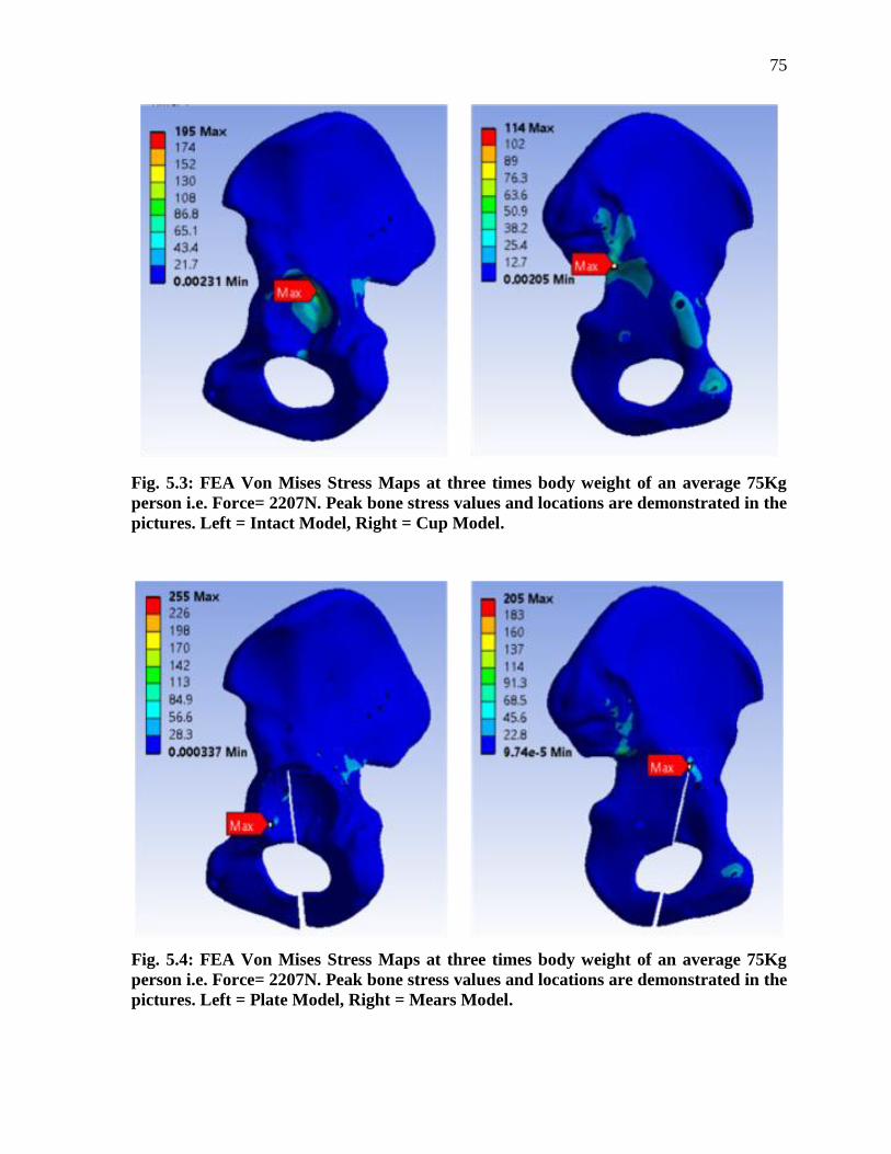
75

Fig. 5.3: FEA Von Mises Stress Maps at three times body weight of an average 75Kg

person i.e. Force= 2207N. Peak bone stress values and locations are demonstrated in the

pictures. Left = Intact Model, Right = Cup Model.

Fig. 5.4: FEA Von Mises Stress Maps at three times body weight of an average 75Kg

person i.e. Force= 2207N. Peak bone stress values and locations are demonstrated in the

pictures. Left = Plate Model, Right = Mears Model.

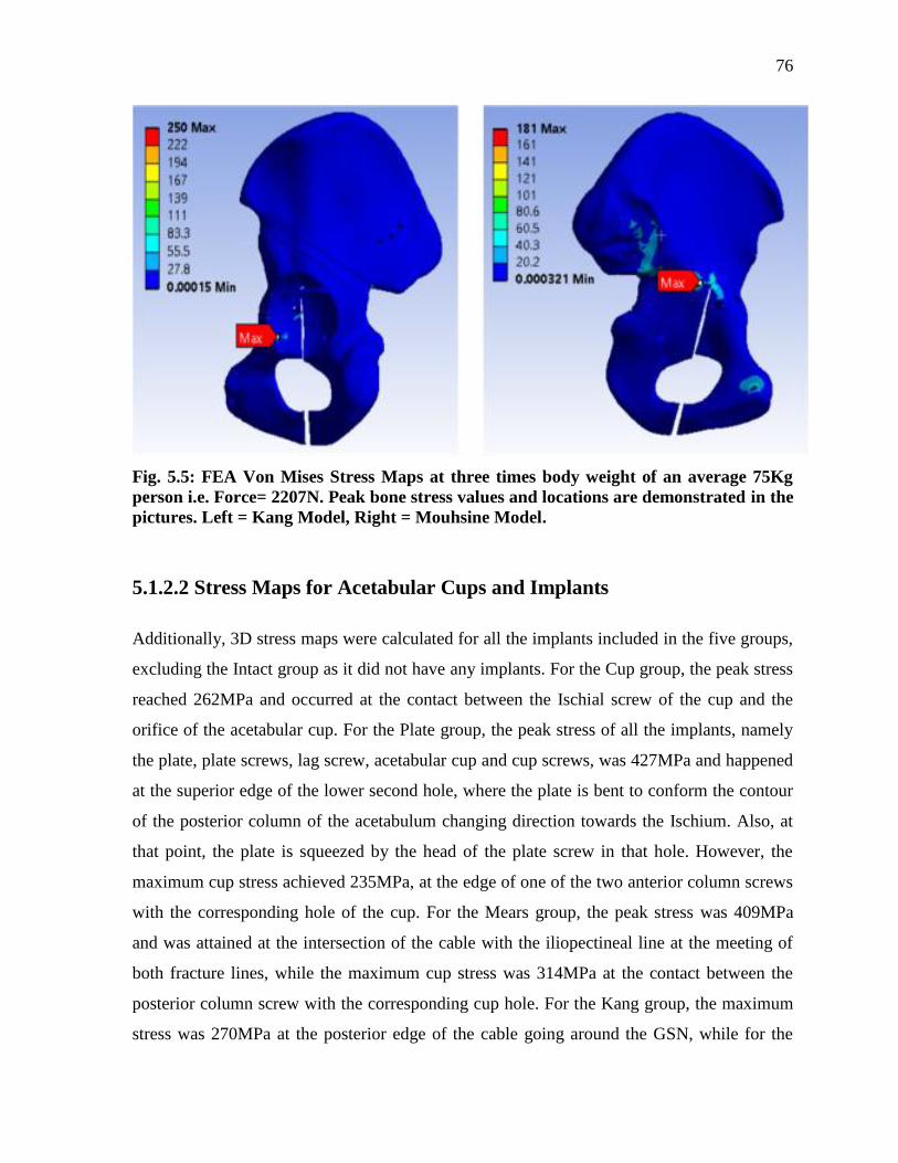
76

Fig. 5.5: FEA Von Mises Stress Maps at three times body weight of an average 75Kg

person i.e. Force= 2207N. Peak bone stress values and locations are demonstrated in the

pictures. Left = Kang Model, Right = Mouhsine Model.

5.1.2.2 Stress Maps for Acetabular Cups and Implants

Additionally, 3D stress maps were calculated for all the implants included in the five groups,

excluding the Intact group as it did not have any implants. For the Cup group, the peak stress

reached 262MPa and occurred at the contact between the Ischial screw of the cup and the

orifice of the acetabular cup. For the Plate group, the peak stress of all the implants, namely

the plate, plate screws, lag screw, acetabular cup and cup screws, was 427MPa and happened

at the superior edge of the lower second hole, where the plate is bent to conform the contour

of the posterior column of the acetabulum changing direction towards the Ischium. Also, at

that point, the plate is squeezed by the head of the plate screw in that hole. However, the

maximum cup stress achieved 235MPa, at the edge of one of the two anterior column screws

with the corresponding hole of the cup. For the Mears group, the peak stress was 409MPa

and was attained at the intersection of the cable with the iliopectineal line at the meeting of

both fracture lines, while the maximum cup stress was 314MPa at the contact between the

posterior column screw with the corresponding cup hole. For the Kang group, the maximum

stress was 270MPa at the posterior edge of the cable going around the GSN, while for the

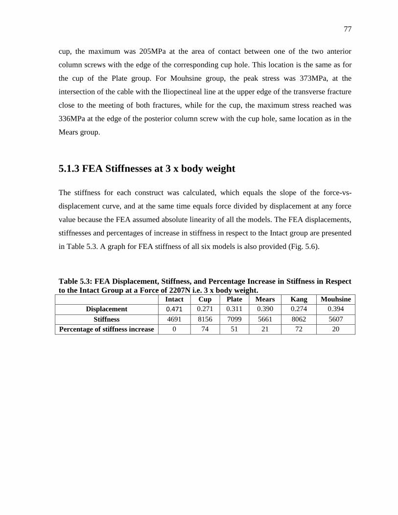
77

cup, the maximum was 205MPa at the area of contact between one of the two anterior

column screws with the edge of the corresponding cup hole. This location is the same as for

the cup of the Plate group. For Mouhsine group, the peak stress was 373MPa, at the

intersection of the cable with the Iliopectineal line at the upper edge of the transverse fracture

close to the meeting of both fractures, while for the cup, the maximum stress reached was

336MPa at the edge of the posterior column screw with the cup hole, same location as in the

Mears group.

5.1.3 FEA Stiffnesses at 3 x body weight

The stiffness for each construct was calculated, which equals the slope of the force-vs-

displacement curve, and at the same time equals force divided by displacement at any force

value because the FEA assumed absolute linearity of all the models. The FEA displacements,

stiffnesses and percentages of increase in stiffness in respect to the Intact group are presented

in Table 5.3. A graph for FEA stiffness of all six models is also provided (Fig. 5.6).

Table 5.3: FEA Displacement, Stiffness, and Percentage Increase in Stiffness in Respect

to the Intact Group at a Force of 2207N i.e. 3 x body weight. Intact Cup Plate Mears Kang Mouhsine

Displacement 0.471 0.271 0.311 0.390 0.274 0.394

Stiffness 4691 8156 7099 5661 8062 5607

Percentage of stiffness increase 0 74 51 21 72 20

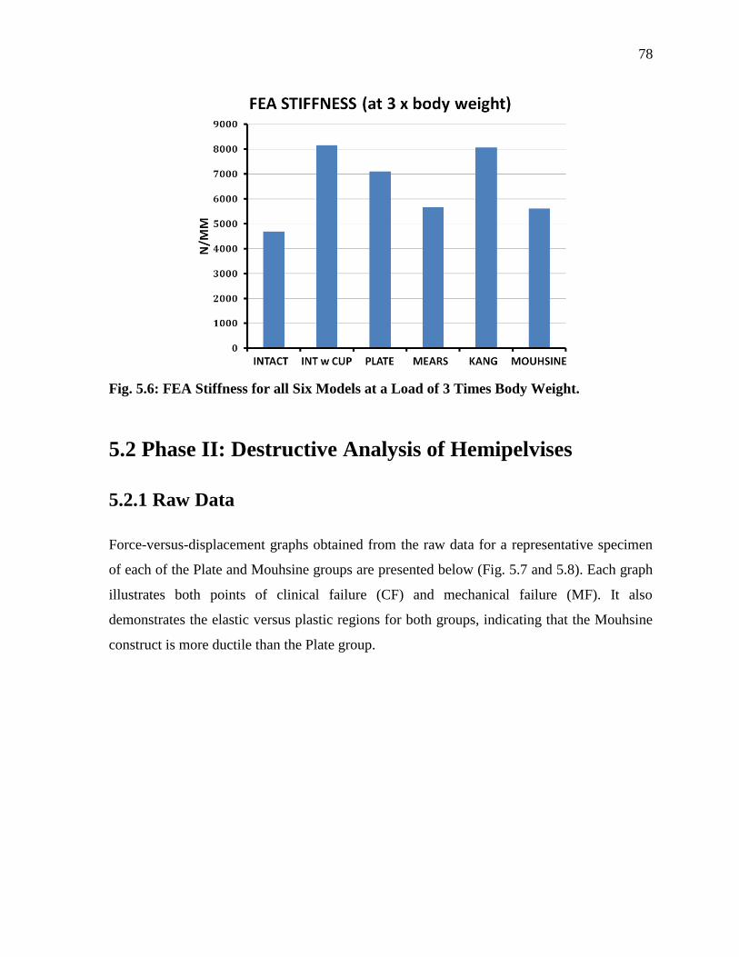
78

Fig. 5.6: FEA Stiffness for all Six Models at a Load of 3 Times Body Weight.

5.2 Phase II: Destructive Analysis of Hemipelvises

5.2.1 Raw Data

Force-versus-displacement graphs obtained from the raw data for a representative specimen

of each of the Plate and Mouhsine groups are presented below (Fig. 5.7 and 5.8). Each graph

illustrates both points of clinical failure (CF) and mechanical failure (MF). It also

demonstrates the elastic versus plastic regions for both groups, indicating that the Mouhsine

construct is more ductile than the Plate group.

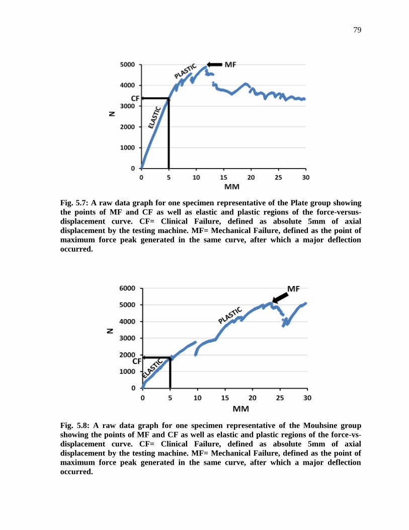
79

Fig. 5.7: A raw data graph for one specimen representative of the Plate group showing

the points of MF and CF as well as elastic and plastic regions of the force-versus-

displacement curve. CF= Clinical Failure, defined as absolute 5mm of axial

displacement by the testing machine. MF= Mechanical Failure, defined as the point of

maximum force peak generated in the same curve, after which a major deflection

occurred.

Fig. 5.8: A raw data graph for one specimen representative of the Mouhsine group

showing the points of MF and CF as well as elastic and plastic regions of the force-vs-

displacement curve. CF= Clinical Failure, defined as absolute 5mm of axial

displacement by the testing machine. MF= Mechanical Failure, defined as the point of

maximum force peak generated in the same curve, after which a major deflection

occurred.

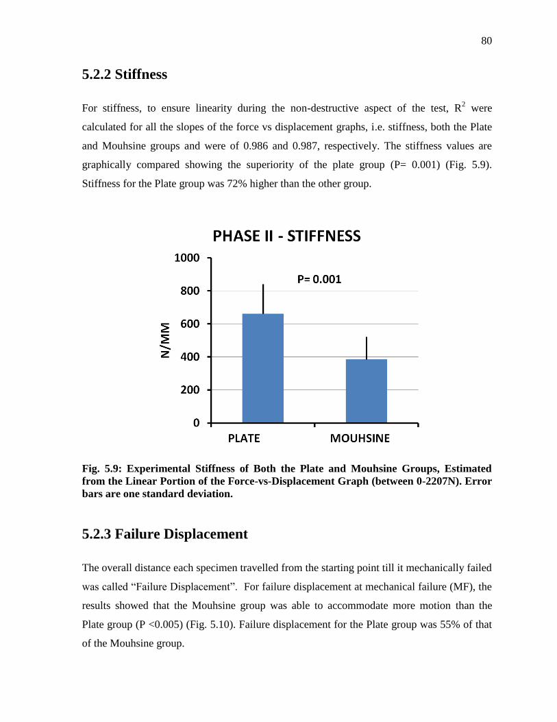
80

5.2.2 Stiffness

For stiffness, to ensure linearity during the non-destructive aspect of the test, R2 were

calculated for all the slopes of the force vs displacement graphs, i.e. stiffness, both the Plate

and Mouhsine groups and were of 0.986 and 0.987, respectively. The stiffness values are

graphically compared showing the superiority of the plate group (P= 0.001) (Fig. 5.9).

Stiffness for the Plate group was 72% higher than the other group.

Fig. 5.9: Experimental Stiffness of Both the Plate and Mouhsine Groups, Estimated

from the Linear Portion of the Force-vs-Displacement Graph (between 0-2207N). Error

bars are one standard deviation.

5.2.3 Failure Displacement

The overall distance each specimen travelled from the starting point till it mechanically failed

was called “Failure Displacement”. For failure displacement at mechanical failure (MF), the

results showed that the Mouhsine group was able to accommodate more motion than the

Plate group (P <0.005) (Fig. 5.10). Failure displacement for the Plate group was 55% of that

of the Mouhsine group.

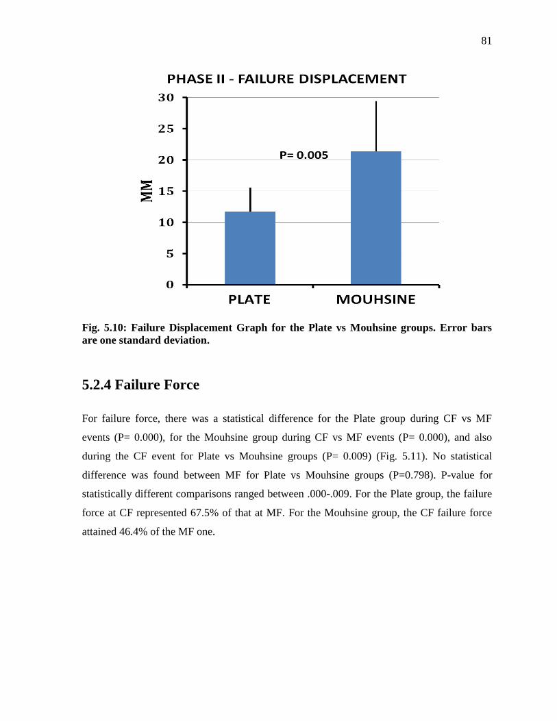
81

Fig. 5.10: Failure Displacement Graph for the Plate vs Mouhsine groups. Error bars

are one standard deviation.

5.2.4 Failure Force

For failure force, there was a statistical difference for the Plate group during CF vs MF

events (P= 0.000), for the Mouhsine group during CF vs MF events (P= 0.000), and also

during the CF event for Plate vs Mouhsine groups (P= 0.009) (Fig. 5.11). No statistical

difference was found between MF for Plate vs Mouhsine groups (P=0.798). P-value for

statistically different comparisons ranged between .000-.009. For the Plate group, the failure

force at CF represented 67.5% of that at MF. For the Mouhsine group, the CF failure force

attained 46.4% of the MF one.

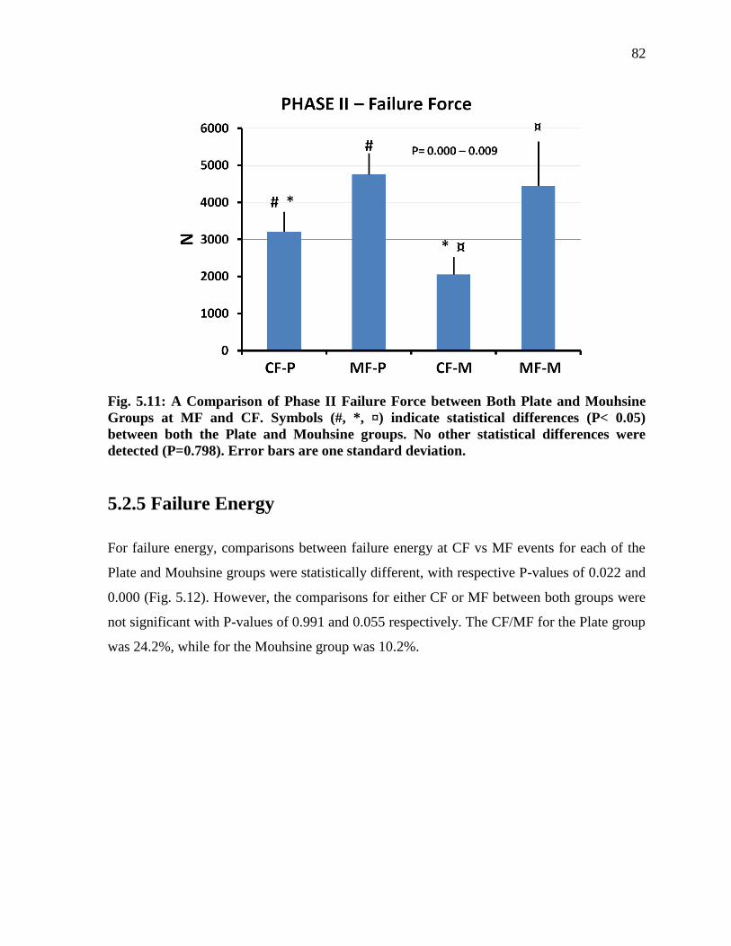
82

Fig. 5.11: A Comparison of Phase II Failure Force between Both Plate and Mouhsine

Groups at MF and CF. Symbols (#, *, ¤) indicate statistical differences (P< 0.05)

between both the Plate and Mouhsine groups. No other statistical differences were

detected (P=0.798). Error bars are one standard deviation.

5.2.5 Failure Energy

For failure energy, comparisons between failure energy at CF vs MF events for each of the

Plate and Mouhsine groups were statistically different, with respective P-values of 0.022 and

0.000 (Fig. 5.12). However, the comparisons for either CF or MF between both groups were

not significant with P-values of 0.991 and 0.055 respectively. The CF/MF for the Plate group

was 24.2%, while for the Mouhsine group was 10.2%.

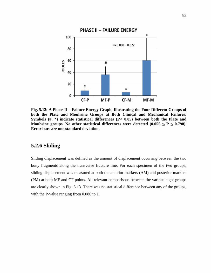
83

Fig. 5.12: A Phase II – Failure Energy Graph, Illustrating the Four Different Groups of

both the Plate and Mouhsine Groups at Both Clinical and Mechanical Failures.

Symbols (#, *) indicate statistical differences (P< 0.05) between both the Plate and

Mouhsine groups. No other statistical differences were detected (0.055 ≤ P ≤ 0.798).

Error bars are one standard deviation.

5.2.6 Sliding

Sliding displacement was defined as the amount of displacement occurring between the two

bony fragments along the transverse fracture line. For each specimen of the two groups,

sliding displacement was measured at both the anterior markers (AM) and posterior markers

(PM) at both MF and CF points. All relevant comparisons between the various eight groups

are clearly shown in Fig. 5.13. There was no statistical difference between any of the groups,

with the P-value ranging from 0.086 to 1.

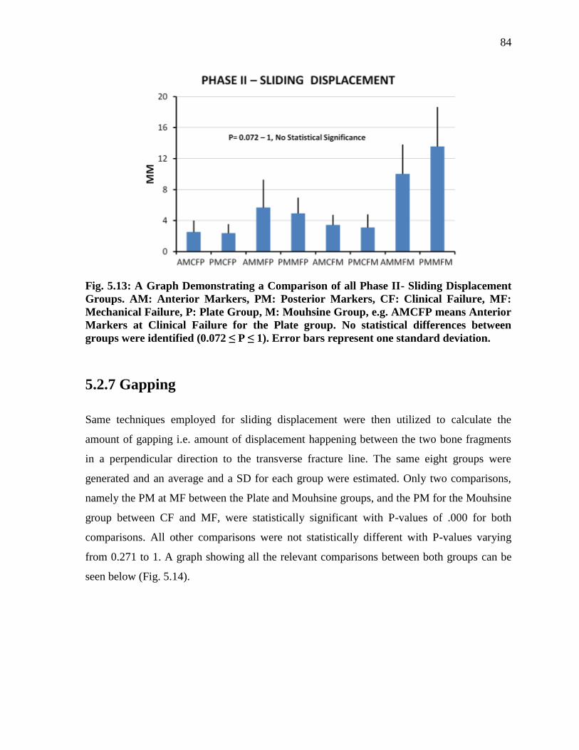
84

Fig. 5.13: A Graph Demonstrating a Comparison of all Phase II- Sliding Displacement

Groups. AM: Anterior Markers, PM: Posterior Markers, CF: Clinical Failure, MF:

Mechanical Failure, P: Plate Group, M: Mouhsine Group, e.g. AMCFP means Anterior

Markers at Clinical Failure for the Plate group. No statistical differences between

groups were identified (0.072 ≤ P ≤ 1). Error bars represent one standard deviation.

5.2.7 Gapping

Same techniques employed for sliding displacement were then utilized to calculate the

amount of gapping i.e. amount of displacement happening between the two bone fragments

in a perpendicular direction to the transverse fracture line. The same eight groups were

generated and an average and a SD for each group were estimated. Only two comparisons,

namely the PM at MF between the Plate and Mouhsine groups, and the PM for the Mouhsine

group between CF and MF, were statistically significant with P-values of .000 for both

comparisons. All other comparisons were not statistically different with P-values varying

from 0.271 to 1. A graph showing all the relevant comparisons between both groups can be

seen below (Fig. 5.14).

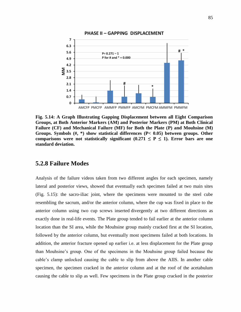
85

Fig. 5.14: A Graph Illustrating Gapping Displacement between all Eight Comparison

Groups, at Both Anterior Markers (AM) and Posterior Markers (PM) at Both Clinical

Failure (CF) and Mechanical Failure (MF) for Both the Plate (P) and Mouhsine (M)

Groups. Symbols (#, *) show statistical differences (P< 0.05) between groups. Other

comparisons were not statistically significant (0.271 ≤ P ≤ 1). Error bars are one

standard deviation.

5.2.8 Failure Modes

Analysis of the failure videos taken from two different angles for each specimen, namely

lateral and posterior views, showed that eventually each specimen failed at two main sites

(Fig. 5.15): the sacro-iliac joint, where the specimens were mounted to the steel cube

resembling the sacrum, and/or the anterior column, where the cup was fixed in place to the

anterior column using two cup screws inserted divergently at two different directions as

exactly done in real-life events. The Plate group tended to fail earlier at the anterior column

location than the SI area, while the Mouhsine group mainly cracked first at the SI location,

followed by the anterior column, but eventually most specimens failed at both locations. In

addition, the anterior fracture opened up earlier i.e. at less displacement for the Plate group

than Mouhsine’s group. One of the specimens in the Mouhsine group failed because the

cable’s clamp unlocked causing the cable to slip from above the AIIS. In another cable

specimen, the specimen cracked in the anterior column and at the roof of the acetabulum

causing the cable to slip as well. Few specimens in the Plate group cracked in the posterior

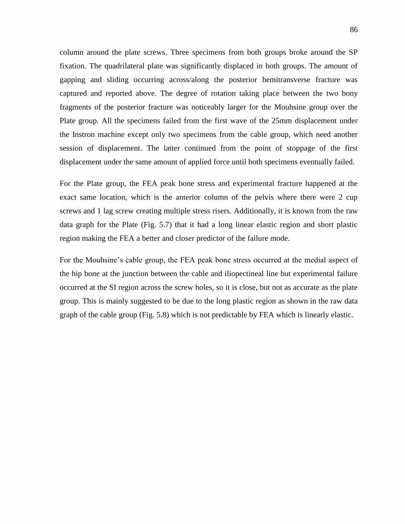
86

column around the plate screws. Three specimens from both groups broke around the SP

fixation. The quadrilateral plate was significantly displaced in both groups. The amount of

gapping and sliding occurring across/along the posterior hemitransverse fracture was

captured and reported above. The degree of rotation taking place between the two bony

fragments of the posterior fracture was noticeably larger for the Mouhsine group over the

Plate group. All the specimens failed from the first wave of the 25mm displacement under

the Instron machine except only two specimens from the cable group, which need another

session of displacement. The latter continued from the point of stoppage of the first

displacement under the same amount of applied force until both specimens eventually failed.

For the Plate group, the FEA peak bone stress and experimental fracture happened at the

exact same location, which is the anterior column of the pelvis where there were 2 cup

screws and 1 lag screw creating multiple stress risers. Additionally, it is known from the raw

data graph for the Plate (Fig. 5.7) that it had a long linear elastic region and short plastic

region making the FEA a better and closer predictor of the failure mode.

For the Mouhsine’s cable group, the FEA peak bone stress occurred at the medial aspect of

the hip bone at the junction between the cable and iliopectineal line but experimental failure

occurred at the SI region across the screw holes, so it is close, but not as accurate as the plate

group. This is mainly suggested to be due to the long plastic region as shown in the raw data

graph of the cable group (Fig. 5.8) which is not predictable by FEA which is linearly elastic.

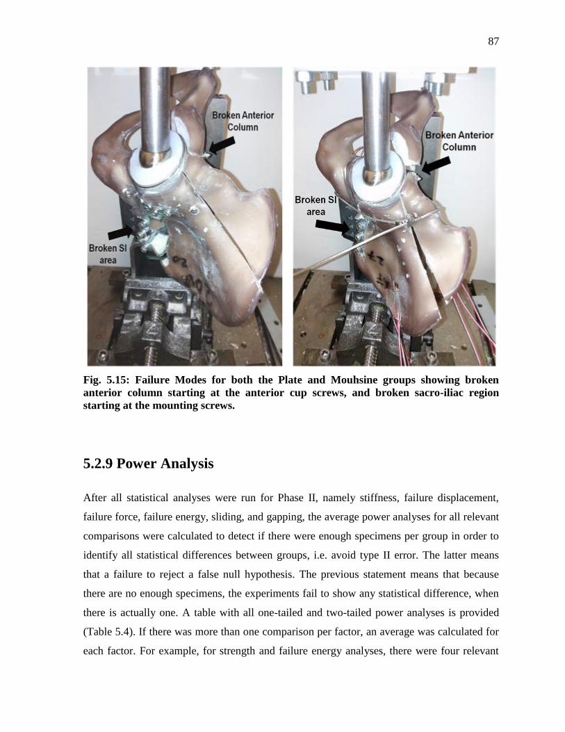
87

Fig. 5.15: Failure Modes for both the Plate and Mouhsine groups showing broken

anterior column starting at the anterior cup screws, and broken sacro-iliac region

starting at the mounting screws.

5.2.9 Power Analysis

After all statistical analyses were run for Phase II, namely stiffness, failure displacement,

failure force, failure energy, sliding, and gapping, the average power analyses for all relevant

comparisons were calculated to detect if there were enough specimens per group in order to

identify all statistical differences between groups, i.e. avoid type II error. The latter means

that a failure to reject a false null hypothesis. The previous statement means that because

there are no enough specimens, the experiments fail to show any statistical difference, when

there is actually one. A table with all one-tailed and two-tailed power analyses is provided

(Table 5.4). If there was more than one comparison per factor, an average was calculated for

each factor. For example, for strength and failure energy analyses, there were four relevant

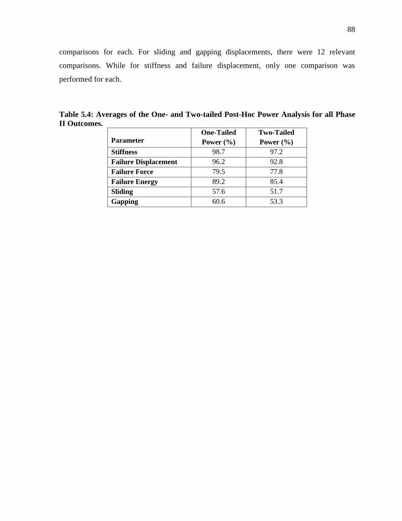
88

comparisons for each. For sliding and gapping displacements, there were 12 relevant

comparisons. While for stiffness and failure displacement, only one comparison was

performed for each.

Table 5.4: Averages of the One- and Two-tailed Post-Hoc Power Analysis for all Phase

II Outcomes.

Parameter One-Tailed

Power (%)

Two-Tailed

Power (%)

Stiffness 98.7 97.2

Failure Displacement 96.2 92.8

Failure Force 79.5 77.8

Failure Energy 89.2 85.4

Sliding 57.6 51.7

Gapping 60.6 53.3

89

Chapter 6

Discussion

6.1 General Findings

This study is the first to assess the biomechanical effectiveness of different surgical fixation

methods for the AHT associated acetabular fracture, which is considered the typical fragility

acetabular fracture pattern seen in the elderly based on experts’ opinion and other

epidemiological studies (Culemann et al., 2010; Ferguson et al., 2010; Hessmann et al.,

2002).

This analysis provided valuable data about the biomechanical stability of employing three

widely used cabling techniques described by Mears and Shirahama (1998), Kang and Min

(2002), and Mouhsine et al. (2002) in fixing complex acetabular fractures. No previous

biomechanical studies ever assessed the usage of cables in fixing any type of acetabular

fractures, making this study a good foundational investigation.

At present, Phase I non-destructive evaluations identified the Mouhsine method as providing

the best mechanical stability (i.e. based on lowest peak bone stress) among the cable

techniques. Phase II destructive assessments demonstrated the Plate group’s superiority over

the Mouhsine group for 2 outcome measurements (i.e. stiffness and failure force at clinical

failure), failed earlier for 2 outcomes (i.e. failure displacement and gapping for posterior

markers at mechanical failure), and had statistical equivalence for the remaining outcomes.

6.2 Comparison to Prior Biomechanical Studies

It is important to place present results into a broader context by comparison to other studies,

where possible (Table 6.1). However, it is difficult to do so because of the large divergence

among biomechanical studies on fractured pelvises. First, different types of specimens were

used for each study, e.g. various cadavers with a wide range of ages and BMDs (Chang et al.,

2001; Culemann et al., 2010; Mehin et al., 2009; Sawaguchi et al., 1984; Simonian et al.,

90

1995; Wu et al., 2013), and also variable synthetic bones (Culemann et al., 2010; Gililland et

al., 2013; Khajavi et al., 2010; Shazar et al., 1998). Second, various force application

techniques were used; some used direct force application on the acetabulum simulating the

femoral head (Chang et al., 2001; Gililland et al., 2013; Khajavi et al, 2010; Mehin et al.,

2009; Shazar et al., 1998), while others applied force indirectly through the fourth or fifth

vertebral body transmitted through the sacrum to the pelvis, resembling reactionary joint

forces (Culemann et al., 2010; Sawaguchi et al., 1984; Simonian et al., 1995; Wu et al.,

2013). Third, specimen preparation differed from one study to another, especially when

cadavers were employed, e.g. some studies used a full pelvis with both sides attached with

anatomical ligaments, including proximal 1/4th

or 1/3th

of the femurs, meanwhile others just

used hemipelvises covering the full range of different possibilities in between. Fourth,

specimen orientations, experimental setups, and testing machines utilized were variable. For

some studies, the specimens were oriented 45° superomedially and 15° posteriorly in the

sagittal section simulating the position of the femoral neck in the standing position (Chang et

al., 2001; Shazar et al., 1998), others used 25° of posterior orientation instead (Khajavi et al.,

2010), some applied force directly perpendicular to the acetabulum (Mehin et al., 2009), and

others simulated normal walking (6.5° flexion, 7.2° abduction) and descending stairs (9.2°

extension, 9.5° abduction) modes (Gililland et al., 2013). Fifth, a huge spectrum of loads was

applied on the specimens to detect stiffnesses or displacements ranging from 150 N to 2000

N. Also, some authors used quasi-static loading, while others used cyclical loading with

different frequencies ranging from 0.25 Hz to 1 Hz. Sixth, various outcomes were sought

from each study varying from axial stiffnesses, yield strengths, maximum strengths, overall

displacements, directional displacements, e.g. gapping, sliding, and rotational displacements.

Seventh, different definitions were used for the same parameter, e.g. strength was considered

by some to be the ultimate failure force (Chang et al., 2001; Gilliland et al., 2013; Shazar et

al., 1998), while others considered CF to occur at 2mm gap of the fracture line and MF to be

the end of the linear portion of the force-vs-displacement curve (Mehin et al., 2009). The

latter was considered yield strength by others (Chang et al., 2001). Eighth, different fracture

types and fixation methods, even for the same fracture type, were examined. Most were done

on elementary types of acetabular fractures, either a pure transverse or a posterior wall

fracture. Finally, no prior studies used the conventional posterior column plate with an

91

anterior column lag screw to fix AHT fractures, and no biomechanical studies assessed the

biomechanical stability of cable fixation for any type of acetabular fractures, a surgical

method that is well known and practiced worldwide.

The only available biomechanical study on the fixation of the AHT fracture pattern was done

by Culemann et al. (2010), which may be the most comparable to the present study. It

provided a comparison of four different fixation methods; two non-locking implants and two

locking-implants utilizing both synthetic and cadaveric specimens. The authors measured the

main displacement occurring at a point located at the inner wall of the posterior column i.e.

on the quadrilateral plate anterior to the anterior border of GSN, as their primary outcome

comparing all non-locking implants together and also locking-implants. However, Culemann

et al.’s study had several substantial limitations, which have been addressed by the present

investigation. First and most importantly, they used only one specimen for each fixation

method, thereby not allowing for proper statistical comparison between groups and

potentially biasing the final results due to accidental superior surgical performance of one of

the specimens. Second, they did not calculate or report any stiffness results for the four

constructs, they only presented displacement as their ultimate result. Third, they wanted to

see the effect of an extra posterior column long periarticular screw on the stability of the

standard plate, so instead of starting with one screw and increasing the number to three

screws (two in the anterior column and one in the posterior column), they inserted three

screws and tested the specimen, then removed two screws (one from the anterior column and

one from the posterior column) and then tested with only one screw. This means they had

two wide and deep periarticular holes that were empty, which might introduce stress risers

and significantly affect the results. Fourth, they did not report the results for some of their

tests, e.g. when they tested the standard plate with only two periarticular screws, and also

displacement at the posterior hemitransverse fracture. Fifth, the fracture they created is not a

typical high anterior column with a posterior hemitransverse fracture pattern, as fully

described by Letournel and Judet (1981). Sixth, the authors did not demonstrate how they

mounted the specimen on the testing machine and how exactly they applied the load.

Seventh, they did not provide pictures of the lateral view of the acetabulum for the reader to

examine how accurate the fixation screws for the locking plates were inserted and if any of

them penetrated the joint area. This omission is noteworthy since, for locking plates, screw

92

direction cannot be really controlled as it is predetermined by the orientation of the plate

itself. Finally, only one loading cycle of subclinical loads was used, i.e. 750 N for synthetic

and 375 N for cadaveric specimens.

Table 6.1: A general comparison of the outcomes of some biomechanical studies

performed on acetabular fractures presenting the conventional methods used.

Study Strength (N) Stiffness (N/mm) Macro-Motion (mm)

Current study

(Plate method) CF= 3210±543

¶

MF= 4753±574

662±180 Sliding at CF:

AM= 2.55±1.49

PM= 2.40±1.16

Sliding at MF:

AM= 5.70±3.59

PM= 4.95±2.03

Gapping at CF:

AM= 0.42±0.52

PM= 0.07±0.65

Gapping at MF:

AM= 1.38±1.15

PM= 0.72±1.23

Current Study

(Mouhsine

method)

CF= 2060±475

MF= 4443±1202

386±137 Sliding at CF:

AM= 3.45±1.31

PM= 3.12±1.69

Sliding at MF:

AM= 10.02±3.82

PM= 13.58±5.09

Gapping at CF:

AM= 1.09±0.93

PM= 0.70±0.90

Gapping at MF:

AM= 4.44±2.18

PM= 4.72±0.82

Chang et al.,

2001 0.95±0.36MPa

║,

Yield strength=

0.84±0.25MPa

2.94±1.23 MPa

(until-failure loading)

----------

Shazar et al.,

1998

--------- ACP=600±242,

ACPLS=960±83,

PCPLS=3130±841*

(until-failure loading)

using markers, values not

reported

Mehin et al.,

2009 CF=848±805

#

MF=1012±557#

456±468

(cyclic loading 50-250N)

Max gap= 0.4±0.5mm

Rotation at CF=1.8°±0.6, at

MF=3.4±1.8

using Infrared LED

Khajavi et al.,

2010

------------ 510±59

(cyclic loading from 0-

2000N)

Combination of sliding and

gapping (mostly sliding)

AM= 2.1±0.6

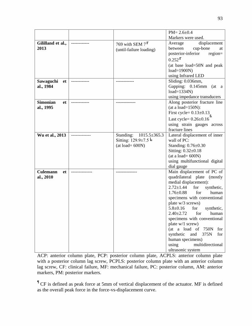
93

PM= 2.6±0.4

Markers were used.

Gililland et al.,

2013

------------ 769 with SEM 7╓

(until-failure loading)

Average displacement

between cup-bone at

posterior-inferior region=

0.252╓

(at base load=50N and peak

load=1900N)

using Infrared LED

Sawaguchi et

al., 1984

------------ ------------ Sliding: 0.036mm,

Gapping: 0.145mm (at a

load=1334N)

using impedance transducers

Simonian et

al., 1995

------------ ------------- Along posterior fracture line

(at a load=150N):

First cycle= 0.13±0.13

Last cycle= 0.26±0.16╚

using strain gauges across

fracture lines

Wu et al., 2013 ------------- Standing: 1015.5±365.3

Sitting: 129.9±7.5╘

(at load= 600N)

Lateral displacement of inner

wall of PC:

Standing: 0.76±0.30

Sitting: 0.32±0.18

(at a load= 600N)

using multifunctional digital

dial gauge

Culemann et

al., 2010

-------------- -------------- Main displacement of PC of

quadrilateral plate (mostly

medial displacement):

2.72±1.44 for synthetic,

1.76±0.88 for human

specimens with conventional

plate w/3 screws)

5.8±0.16 for synthetic,

2.40±2.72 for human

specimens with conventional

plate w/1 screw)

(at a load of 750N for

synthetic and 375N for

human specimens)

using multidirectional

ultrasonic system

ACP: anterior column plate, PCP: posterior column plate, ACPLS: anterior column plate

with a posterior column lag screw, PCPLS: posterior column plate with an anterior column

lag screw, CF: clinical failure, MF: mechanical failure, PC: posterior column, AM: anterior

markers, PM: posterior markers.

¶ CF is defined as peak force at 5mm of vertical displacement of the actuator. MF is defined

as the overall peak force in the force-vs-displacement curve.

94

║ All measures for strength and stiffness were in MPa (incorrect). Failure occurred most of

the times around the two lower screws of the plate.

* Calculated stiffness for PCPLS from anterior displacement (giving higher values). # Authors defined CF as failure happening at 2mm gap and MF as failure occurring at the end

of the linear portion of force-vs-displacement curve. ╓

Only two specimens were used. All specimens failed at the sacro-iliac mounting holes. ╚

Type of displacement was not identified whether it was gapping, sliding, or rotation.

╘ Mostly due to errors in the anterior displacements happening in the sitting position, which

were not presented in the study. Displacements were not specified (gapping, sliding, or

rotation).

6.3 Biomechanical Implications

Phase I results have several salient implications on the initial biomechanical stability of AHT

fracture fixation prior to any significant weight bearing.

FEA showed that the acetabular cup increased the overall stiffness by 74% and decreased the

peak bone stress by 42% in respect to the “Intact” control. This finding assists in

understanding one of the many reasons for the great long-term success achieved by currently

available acetabular cups. The latter has also an outer porous surface at the micro-level to

stimulate the migration and activation of osteoblasts to its surface encouraging “contact

osteogenesis” i.e. bone growth and interdigitation with the implant surface with no micro-

gaps between the prosthesis and the newly-formed bone leading to better biomechanical

stability (Davies, 2003)

FEA demonstrated that all fixation methods provided stiffnesses higher than the Intact group,

with the Mouhsine group being the lowest offering 20% increase in stiffness than the Intact

specimens, which means they are potentially acceptable ways for fixing acetabular fractures.

It is also noticeable that the Plate and Kang groups achieved very similar values and

locations of stiffness and peak bone stress results, meanwhile the stiffness and stress maps

for the Mears and Mouhsine groups were alike, employing that each of these two methods

can be theoretically applied interchangeably with accomplishing almost the same successful

results. Additionally, it was shown that all the four methods provided good biomechanical

stability for the immediate post-operative state handling stress applied on the bone from a

95

range of 1 ¼ body weights for the Plate group being the lowest to 1 ¾ times body weight for

the Mouhsine group, when the peak bone stress attains 106MPa i.e. the maximum tolerable

value for tensile strength before the cortical shell starts cracking. These values are by far

higher than the actual amount of force needed to be applied in the first few weeks after

surgery, which usually reaches only 10% of the body weight (Simonian et al., 1995) allowing

for good fixation of bone fragments and giving them the chance to fully and properly heal

together. Graded increase of load-bearing then follows till it reaches full weight bearing 12

weeks post-operatively.

“Stress Shielding” theory affirms that the stiffer the implant is, the higher the load the

implant carries. This would lead to lesser load being transferred from the implant to the bone,

producing less stress on the bone causing eventual bone resorption, implant loosening, and

failure. The Plate technique, which is mainly dependent on bone/screw interaction for both

the fixation of the plate and the lag screw, may be more affected by the stress shielding

theory than the cabling technique, which mainly relies on the outer compression of bony

fragments together rather than bone/implant interface. Consequently, even if bone loosening

happens on the micro-scale, it would minimally affect the biomechanical stability offered by

cables. Furthermore, as clearly seen from the FEA, the Mouhsine cabling technique

generated better stress distribution of the bone, being wrapped all around the hip bone, as

illustrated by a 30% decrease in the peak bone stress, yielding 181MPa vs 255MPa for the

Plate group at a force of three times body weight i.e. 2207N. Even at lower force values, the

ratio between peak bone stresses for both groups remains constant because the FEA assumes

absolute linearity.

Phase II results also have several important implications on the biomechanical stability of

AHT fracture fixation after significant weight bearing is introduced, which could lead to

failure.

The Mouhsine cable method currently demonstrated statistical equivalence to the

conventional Plate technique for a number of biomechanical outcomes, suggesting it is a

feasible surgical approach. This is in agreement with Mouhsine et al.’s report on the clinical

outcomes of this procedure in the presence of an acute THA in 18 older patients (average age

96

of 76 years) for a mean follow-up of three years. The report showed that the functional

outcome of the patients was excellent in 65% of the cases and good for 35%. The mean hip

motion was 108° of flexion and 12° of extension, 32° of internal rotation and 35° of external

rotation, and 30° of abduction and 26° of adduction. Radiologically, 88% of the patients

showed no radiolucency, while 12% had a less than 1mm central radiolucency. All fractures

healed with 87% of the patients having an average of 2.3mm superior and 2mm medial

migration of the acetabular cup, which happened in the first three month post-operatively and

stabilized afterwards. Heterotopic ossification of Brooker grade I was noted in 35% of the

patients. These results are comparable to the results reported in the literature for various

fixation techniques in elderly patients with displaced acetabular fractures (Mears and

Velyvis, 2002; Sarker et al., 2004; Tidermark et al., 2003).

The Plate group was much stiffer than the Mouhsine group presenting 72% increase in the

overall construct stiffness, which would lead to better immediate post-operative stability.

Accordingly, with the same force applied on both groups e.g. bedside activities or

rehabilitation, more movement between the bone fragments will occur in the case of the

Mouhsine group than the Plate group, which may endanger bone healing. Previous clinical

and biomechanical studies reported that the higher the stiffness of the applied implant would

lead to higher overall stiffness of the construct, which would lead to better fracture stability

in the recent post-operative period i.e. before bone healing occurred (Dennis et al., 2001;

Fulkerson et al., 2006; Lever et al., 2010; Peters et al., 2003; Schmotzer et al., 1996; Talbot

et al., 2008; Wilson et al., 2005; Zdero et al., 2008b).

Regarding failure force results of both groups at the CF event, where the Plate group was

1.56 times stronger than the Mouhsine group, implies that more load needs to be applied on

the Plate specimens in order to achieve the same amount of displacement taking place in the

Mouhsine group. The same trend was also confirmed by investigating the MF results for both

groups, where the Plate group achieved higher failure strength, though not statistically

significant, with much lower failure displacement only constituting almost a half i.e. 55% of

its counterpart at the Mouhsine group (P=0.005). This might give the impression that the

Plate method is superior. However, this is not necessarily the case for elderly (osteoporotic)

patients, who have fixation of an acetabular fracture accompanied with a THA and are not

97

altogether permitted to put any weight-bearing on their legs for at least the first six weeks

post-operatively to allow for proper bone healing. The reason is that, in the immediate post-

operative interval, all the loads applied are mainly passive movements performed by

physiotherapists, occupational therapists, or nurses, plus any additional bedside movements,

activities, or exercises the patients are asked to do. All these movements would only present

10% of the patient’s body weight (Simonian et al., 1995). As such, it can be observed that for

the Mouhsine group, which is weaker, a load of 2060 N i.e. 2.8 times body weight of an

average 75 kg person, was achieved. This means that a load with the magnitude of 28 times

the force normally generated from the regular post-operative movements is required to

clinically fail the Mouhsine fixation technique. Moreover, considering that there was no

statistical significance in sliding and gapping at CF for either the AM or PM between both

repair groups, it could be recommended that the Mouhsine fixation be applied. This is

because at the very low load applied in the immediate post-surgical condition, a little bit

more micromotion may occur between the bony fragments of the fracture, which might

mechanically stimulate bone osteoblasts to start osteosynthesis earlier and cause better bone

healing and union. The effect of slight micromotion between bone fragments on increasing

the rate of bone healing was proved by some previous clinical in-vivo and in-vitro studies

(Hak et al., 2010).

The Mouhsine group provided almost the same amount of failure force and higher failure

energy (66% increase) at MF vs. the Plate group, even if statistically insignificant. This trend

demonstrates the ductile nature of the cable/bone construct versus the more brittle nature of

the plate/bone implant. Ductility by definition is “a solid material’s ability to deform under

tensile stress”, which demonstrates the material’s capacity to stretch into a wire. Brittleness is

defined as “a material, when subjected to stress, it breaks without significant deformation”.

To clarify, a material may be very strong, but brittle, as it does not absorb much energy

before breaking e.g. ceramics and glass. To apply that on the two constructs, the Mouhsine

group is less stiff, but it deforms substantially, i.e. displacement and absorbs much energy

(long plastic region) before mechanically breaking down, even if it failed clinically much

earlier, resulting in much higher failure energy than the other group. On the other hand, the

Plate group is much stiffer, but not as ductile i.e. brittle, so it is stronger, but does not deform

much (shorter plastic region), and therefore, does not absorb as much energy before failure.

98

Therefore, the amount of displacement at MF with the cable group is much larger, which

consequently lead to more sliding, gapping and rotation. Also, because the plate is always in

contact with the bone in a plane rather than just a line, it was able to restrict rotation along

the posterior component of the fracture, which was not the case with cables because it holds

the bone in just a slender line allowing the potential for rotation, especially under much

displacement because of its ductile properties.

6.4 Surgical Implications

Several technical improvements can be suggested in the use of cables and screws for surgical

practice and future studies based on the current author’s experience during specimen

preparation.

First, two out of 10 cables employed in the Mouhsine fixation method slipped from above the

AIIS at very high loads i.e. above 3500N. This happened in one case mainly because the

clamp screw unlocked allowing lengthening and slippage of the cable. However in the

second case, it was mainly because of breakage of the iliac fragment at the SI region and at

the rim of the acetabulum at the roof causing slippage of the cable from around the AIIS.

Despite that, it would be recommended to drill a small 2.5 or 2.7mm hole at the base of the

AIIS directed from postero-lateral to antero-medial to pass the cable through it, as routinely

done in Mears and Shirahama (1998), in order to secure the cable firmly and prevent any

chances of slippage e.g. in case of a patient stumbling post-operatively and generating a high

and sudden force magnitude at the hip joint.

Second, the Accord cabling system [Smith and Nephew Inc., Memphis, TN, USA] was

employed. However, for both the Mears and Mouhsine techniques a longer course of the

cable around the specimen is required vs. the Kang method, thus the remaining free end of

the cable after passing through the clamp was too short to properly fit in the cable tensioner.

The cable tensioner could not provide gripping of the cable when the “Locking Handle” was

turned clockwise all the way. Therefore, the anterior nozzle (end) of the tensioner was

unscrewed to save some length, and so, the free end of the cable can be inserted deeper into

99

the tensioner allowing a good grip of the tensioner on the cable. A wide washer was used at

the front end of the tensioner to push against the clamp so that the latter does not sink inside

the tensioner, and therefore, the clamp’s screw can be tightened using a surgical screwdriver.

Therefore, it is proposed that either at least 10 cm longer cables (current cable length was

61.2 cm), or cable tensioners that act effectively with much less length (at least 10 cm)

provided by the free end of the cable, should be designed for achieving effectiveness and

comfort to operating surgeons. Furthermore, an Accord clamp taken from another new cable

was used as a supplementary second clamp applied on the quadrilateral plate for the

Mouhsine’s technique. However, this clamp was complex, difficult to pass the end of the

cable twice across, and not meant to be used in the quadrilateral area for that purpose.

Therefore, a simpler two-channel straight second clamp applied on the quadrilateral plate, as

originally described by Mouhsine et al. (2002), needs to be designed for the easier passage of

the cable.

Third, it was noted that for both the Plate and Mouhsine groups, all specimens failed first at

either the sacro-iliac region, or the anterior column around the acetabular component fixation

screws. For the SI region, it was noticed that cracks started at or propagated to the holes of

the mounting screws causing eventually a complete fracture of that area along the line of

fixation, as shown in Fig. 5.15 in the results section. This finding was also reported in

another recent study performed on fixing pure transverse acetabular fractures applying three

different constructs, where all specimens failed at the same region around the mounting holes

as well (Gililland et al., 2013). For failing at the anterior column region, it was clear that the

anterior column of those synthetic hemipelvises, and most likely also applies on human

cadaveric specimens based on experts opinion, was really narrow and was further narrowed

after reaming of the acetabulum to insert an acetabular shell as part of a THA. The diameter

of the anterior column could not handle the passage of a 6.5mm lag screw in the standard

orientation from the outer table of the ilium supra-acetabularly close to the AIIS through the

acetabular component of the ilio-pubis to settle down in the superior pubic ramus close to the

pubic body. Therefore, when this finding was detected in the pilot studies before the start of

the current study, lag screws were changed into 4.0 mm ones instead. Thus, in osteoporotic

patients with displaced acetabular fractures that need primary acute THA, it is advisable not

to use two anterior column screws. One screw in the anterior column may be enough because

100

the anterior column is already weak, narrow, and osteoporotic, and the final lag screw to be

inserted may create added stress risers and predispose the column to fail earlier. It may be

intuitively argued that inserting more screws in the anterior column will make it stronger;

however, because of the narrow area and poor bone quality, installing two large 6.5mm

screws for stabilizing the acetabular cup is replacing a large amount of bone, which is already

scarce, further weakening it. If surgeons are looking for better acetabular component

stability, other large screws can be inserted in the dome of the cup, posteriorly towards the

sciatic buttress, or even inferiorly in the ischium, which all were proven from this study to be

extremely tight and strong and remained in place even after mechanical failure. Based on the

current results, it is recommended that redistribution of the cup screws with just one anterior

column screw and more dome, posterior column, or ischial screws. Otherwise, four 6.5mm

cup screws were enough providing a 74% increase in the overall stiffness and 42% lower

peak bone stress in comparison to the Intact group.

Fourth, the Mouhsine cable method is preferred among the various cable methods examined

from a biomechanical point of view. However, the final decision is left to the operating

surgeon because, from the surgical point of view, cables generally are technically much

difficult to apply than the Plate method. Cabling requires much more stripping, splitting, and

dissection of soft tissues and muscles in the vicinity of many vital structures, such as arteries,

veins, and nerves. Moreover, the Mouhsine method in particular is even more technically

demanding than the other two cable methods. Therefore, successful Mouhsine-type cabling

would require substantial surgical training and practice by a specialized trauma surgical team

to avoid vascular or neural injuries, minimize surrounding soft tissue trauma, and maintain

good circulation in the area, i.e. periosteum, surrounding muscles, and soft tissues, for proper

bone healing.

Fifth, the Mouhsine cabling method provides a great benefit over the Plate group, which is

mechanically supporting the quadrilateral plate, having an extra clamp resting on the

quadrilateral, with four cable ends going all the way across it. This advantage is considered

very important for the success of any acute THA performed as a primary management for

displaced acetabular fractures especially in the elderly, even if using procedures other than

cables for fixing the fracture itself (Sarker et al., 2004). From the stability point of view, the

101

Mouhsine cable method is specifically superior because of the addition of an extra clamp i.e.

sleeve on the quadrilateral plate, which serves as an extra origin for the cable that the more

the tension is applied on the cable e.g. femoral head pushing against the acetabular

component of a THA, the more the compression on the bone is applied. That is because when

the clamp is pushed out by bone under the influence of the applied force, the clamp itself

pulls all the four ends of the cable going through it generating more compression all the way

around the bone compressing the bone fragments together and providing more support to the

quadrilateral plate to keep its integrity and resist displacement i.e. sliding or gapping. That is

referred to as “Tension band” theory.

Finally, From a clinical perspective, stiffness, CF force, and gapping are clinically relevant,

where patient’s pain, discomfort, or functional impairment may start to occur. For stiffness,

the higher the stiffness of the construct, the better the immediate post-operative stability.

Also, a higher CF force means that more force was required to achieve the same amount of

displacement i.e. 5mm. The latter indicates the strength of the construct, and therefore, the

success of the fixation technique. For gapping, it has been previously shown that the better

the fracture reduction with less gaps, the better the healing and clinical outcomes (Matta et

al., 1986; Matta and Merritt, 1988; Matta, 1996).

6.5 Possible Limitations

The limitations of the current study are typical for in-vitro biomechanical studies, which may

have influenced the absolute values of the reported outcomes but not the relative trends.

Synthetic, instead of cadaveric, hemipelvises, were used. Based on their manufacturing

technique (i.e. glass fibers in epoxy resin are mixed thoroughly) and measured mechanical

properties which fall within a relatively small range (i.e. longitudinal vs. transverse vs.

compressive), the synthetic bones supplied by Sawbones are more isotropic and

homogeneous than human bones whose microstructure follows lines of applied stress.

Therefore, the outcomes of the present study need to be validated in future studies versus

fresh frozen human cadaveric hemipelvises to achieve the absolute numbers of the

102

parameters addressed by this study and also confirm the same comparative trend between the

various fixation groups. This limitation may affect the absolute values for the study’s

outcomes causing more variation between the specimens and maybe decreased stiffness and

strength, and increased failure displacement. However, the main reason for the use of

synthetic hemipelvises was that inter-specimen variation of synthetic bones is much lower

than that of cadavers (Cristofolini et al., 1996). Synthetic bones from Sawbones [Vashon,

WA, USA] are also commonly used in many biomechanical studies on long bones such as

femurs, tibias, and humeri (Aziz et al., 2014a,b,c; Bougherara et al., 2009; Ebrahimi et al.,

2012; Shah et al., 2011; Tuncer et al., 2014) and compare reasonably well to human cadavers

for a variety of mechanical properties (Aziz et al., 2014a,b,c; Dennis et al., 2000; Papini et

al., 2007; Zdero et al., 2009) Moreover, the high financial cost, storage requirements,

biotoxicity, and limited access to matched pairs of human hemipelvises made synthetic bones

an attractive option for this study.

Osteoporotic-like synthetic hemipelvises designed based on data obtained from a 45 year old

male were initially planned for the study. There may be no differences in the human anatomy

of the pelvis between younger and older populations, except for thinner cortices, lower BMD,

and increased porosity, where bones of the elderly may become more osteopenic and

sometimes, even osteoporotic.; however, there is very limited data addressing this issue

(Brockstedt et al., 1993; Foldes et al., 1991; Vedi et al., 2011). In light of the current results,

the author expect that using osteoporotic bone would be in favor of the cabling technique,

which mainly depends on compressing the bony fragments together vs. the plating technique,

which primarily employs the bone/screw interactions. However on the other hand, the cables

may also cut through the osteoporotic specimens leading to an early failure. Therefore, the

final conclusions would be based upon completion of a similar study on true osteoporotic

fresh frozen human cadavers. To date, “fully osteoporotic” synthetic hemipelvises are not

commercially available from any medical product manufacturer. Although Sawbones only

produces one standard density and geometry for the cortical shell which simulates normal

bone, the lowest possible density of 0.16 g/cc was chosen for the cancellous matrix to

represent osteoporosis.

103

A quasi-static axial load, instead of cyclic load, was applied for mechanical testing. Cyclic

loading is more physiological as it resembles daily-life activities, e.g. walking, running,

climbing stairs, and playing sports. However, a quasi-static loading minimized visco-elastic

effects, thus producing a more “conservative” result. Also, the long-term fatigue failure of

the different constructs was not assessed, which usually often requires 1 million cycles.

Under repetitive cyclical loading, the fixation implants develop more “mechanical slack”.

The latter would affect the present mechanical results in the form of decreased stiffness and

strength and increased gapping, sliding and rotational displacements. However, the relative

trends between the groups would likely be maintained. For instance, the latter was done by

Simonian et al. (1995), where the displacement across the posterior fracture line of a T-

shaped fracture was 0.13±0.13 in the first cycle and 0.26±0.16mm at the last cycle.

Bone healing was not considered in the scope of this study as the author meant to look at the

biomechanical stability in the immediate post-operative period before any substantial bone

healing and partial weight bearing can take place. To simulate bone healing using FE models,

the fracture gaps could be abolished replicating full bone union as previously done in other

biomechanical studies (Bougherara et al., 2009; Ebrahimi et al., 2012). However, it is very

difficult to simulate progressive degrees of bone healing in in-vitro biomechanical

experimental studies (other than full union) such as those for this study. If bone healing is to

occur, it will affect all the relevant biomechanical outcomes in the sense that it would

probably increase the overall stiffness, load and energy to CF, and decrease the failure

displacement i.e. sliding and gapping.

There are different groups of muscles that act on the hip joint in order to achieve all the wide

spectrum of movements happening across that joint, namely flexion, extension, abduction,

adduction, medial rotation, lateral rotation and circumduction. The main hip flexor is the

psoas muscle, helped by the iliacus. Extension is mainly performed by the gluteus maximus.

Adduction is mainly carried out by the adductor group of muscles. Hip abduction is mainly

exerted by the gluteus medius and minimus. In the current study, the effect of muscles and

surrounding soft tissues on the bone stiffness and stress distribution was not determined.

Bitsakos et al. (2005) showed that the more muscle attachments included in the FE models,

the more bone conserving effect around the THA would eventually result. Stolk et al. (2001)

104

showed that an FE model involving only the abductor muscle force vector can adequately

imitate the mechanics of cemented THA during in vivo loading. Several other studies have

further simplified the process by not simulating any of the muscle groups around the hip joint

(Bougherara et al., 2010a,b, 2011a,b; Davis et al., 2008; Dennis et al., 2000, 2001; Dubov et

al., 2011; Ebrahimi et al., 2012; Fulkerson et al., 2006; Lever et al., 2010; Peters et al., 2003;

Schmotzer et al., 1996; Shah et al., 2011; Stevens et al., 1995; Talbot et al., 2008a,b; Wilson

et al., 2005; Zdero et al., 2008b). Additionally, the FEA in the current thesis was designed to

simulate the exact experimental setup (and not the real life clinical situation) in order for the

experimental results to be adequate for validation of the FEA outcomes. If the abductor force

was modeled in the current study, it would have neutralized some of the stresses applied on

the hip bone decreasing the overall absolute values of Von Mises peak bone stresses;

however, this would not affect the comparative relations between the various fixation

methods. However, this is a typical simplification for in-vitro biomechanical studies, even for

those which use human cadaveric specimens, because soft tissues and muscles are frequently

stripped off the bone.

Almost all the specimens failed during the “mechanical failure” event at or around the

mounting holes of the sacro-iliac region. Although this finding was also reported by another

recent biomechanical study done on transverse acetabular fracture fixation (Gilliland et al.,

2013), it cannot be firmly concluded whether this occurred mainly because the screw holes in

the bone at that region were close to each other or it is a normal finding given the nature of

the test setup.

The AHT fracture was created for the current study by drawing the fracture lines on the exact

location every time and using a jigsaw, the fractures were consistently created in all the

specimens. However, this way of making fractures does not replicate the real-life situations

causing bone fractures. On the other hand, a small drill bit e.g. 1.5mm can be used to drill

some partial-thickness holes along the desired fracture line 2mm apart. By using an

osteotome and applying a force along that line, the fracture can be created in a more realistic

and anatomic manner, but it may be less consistent way because of the increased number of

steps (Simonian et al. 1995).

105

For Phase I a low axial load of 200 N was applied, which is much lower than physiological

loading. A previous biomechanical study on a simple transverse acetabular fracture, dividing

the bone in only two fragments instead of 3, applied a maximum load of 250 N (Mehin et al.,

2009), and another study on a T-shaped acetabular fracture applied an even lower load of 150

N (Simonian et al., 1995). Therefore, low load was intentionally selected to prevent

damaging the specimens during strain gauge measurements, which are meant to remain

within the linear elastic range.

FEA assumes absolute elastic linearity regardless of the amount of load applied. Thus, when

different fixation groups are compared together for relative performance between them,

rather than absolute values reflective of “real life”, the exact same trend between groups is

achieved whether FEA is run far below (i.e. technically correct) or far above (i.e. technically

incorrect) the yield point. Consequently for the present goal of Phase 1, FEA analysis at low

(or high) loads was appropriate and predictive of which repair method would fail earlier and

which would fail later. However, the author did not use the FEA for modeling bone failure,

but to achieve a preliminary idea of how the different fixation groups would behave in

relation to each other until the yield point i.e. the elastic region of the stress-strain curve.

Experimental stiffnesses were lower than FEA stiffnesses since absolute relationships

between parts are assumed for FEA, e.g. for the fixed support regions at SI and SP locations,

FEA assumed no micro-motion in that area, “bonded” contact between SI screws with bone

and steel block by definition have no movement, etc, that do not replicate the mechanical

slack that possibly existed in the experimental setup.

For the validation graph, the correlation coefficient was only R=0.82 and not higher as

previously reported by other biomechanical studies performed on long bones (Bougherara et

al., 2010b; Bougherara et al., 2011b; Dubov et al., 2011; Ebrahimi et al., 2012; Shah et al.,

2011). However, this data scatter was likely caused by a combination of the complex

geometry of the pelvises in comparison to long bones and human error involved in

orientating and mounting specimens. Even so, the slope of the validation graph reached a

value of 1, which represented the accuracy of the FE model vs. experiments.

106

The test setup’s mechanical stiffness was not accounted for in the measured stiffnesses. This

is because the Instron’s mechanical stiffness was 260 kN/mm, which is two orders of

magnitude larger than the measured stiffnesses for all groups in Phase I and II, thereby

eliminating this factor as a confounder.

Rosette strain gauges were chosen, instead of linear gauges, since rosettes are known to be

more suitable for curved surfaces. Unfortunately, some variation in the rosette readings was

noticed, possibly due to the highly complex 3D geometry of the specimens and the presence

of plates, screws, and cables, which can introduce stress risers in the vicinity of the rosettes.

Specimens were over-reamed by 1 mm relative to the diameter of the cup, which would not

be practiced in real-life surgery. However, this was performed because the thickness of the

jigsaw used for cutting the specimens and creating the fracture is almost 1 mm with angled

teeth, which eventually lead to a total loss of bone material of 1 mm. This over-reaming

enabled perfect reduction of fractures even after the insertion of the acetabular shells.

In the Plate group, the lag screw inserted into the anterior column was oriented in the

standard fashion, i.e. textbook version, and not the practical fashion, i.e. daily surgical

practice. This also allowed for practical advantages during specimen preparation for

mechanical testing.

One of the most important factors for the success of the CHP is to provide enough

mechanical stability to allow for bone ingrowth around the acetabular shell, and therefore,

micromotion at the cup bone interface is a very important biomechanical parameter to assess

as done in a prior biomechanical study (Gililland et al., 2013). However, the current study

did not evaluate this outcome for practical issues and absence of the proper equipment

needed for the accurate measurement of the micromotion at the bone/implant interface.

However, the overall stiffness, which represents the total displacement for a given force, as

well as the failure energy at CF, which incorporates both the applied force and the concurrent

displacement, can provide a rough idea about the overall mechanical stability of the fixation

technique around the cup. Also, gapping and sliding along the posterior fracture component

of the AHT can estimate the success of the fixation techniques as discussed before in some

107

clinical studies about displaced acetabular fractures (Matta et al., 1986; Matta and Merritt,

1988; Matta, 1996).

The orientation of the specimen in the setup under the mechanical testing machine did not

allow much access to assess the exact amount of medial displacement of the quadrilateral

plate, i.e. femoral head, which is regarded as the mainstay for the repair of acetabular

fractures using acute primary THA, and is also looked at as a very important category in the

long-term follow-up evaluation of the success of the fixation method performed. Also, this

rigid support might have decreased the medial displacement of the acetabulum. However,

similar rigid support was employed by almost all other biomechanical studies performed on

fixation of pelvic fractures. Additionally, because the same setup and orientation was used

for all the specimens, the relative performance between various groups was not affected.

A more basic measure was taken to assess the displacement occurring along the posterior

fracture line using markers and videotaping the whole displacement process. This procedure

enabled a calculation of sliding and gapping; however, rotation was seen but not measured.

Rotation is deemed to be essential in acetabular fractures because most fractures are mainly

rotated more than translated (Vanderschot, 2007). Other studies employed more sophisticated

techniques in identifying all 3D displacements occurring along one or more areas of the

acetabulum such as infrared LED (Gililland et al., 2013; Mehin et al., 2009), multidirectional

digital dial gauge (Wu et al., 2013), and multidirectional ultrasonic system (Culemann et al.,

2010), which were not readily available in the current study.

Post-hoc power analysis showed that sliding and gapping was below 80%, indicating that the

study was under-powered for these parameters. Thus, not surprisingly, no statistical

difference was noted for these outcomes. However, stiffness, failure displacement, failure

force, and failure energy approached or achieved 80%.

Finally, the current study did not include other methods applied for fixing AHT fractures,

such as the conventional pelvic brim 12-hole long reconstruction plate, locking plates, or

other buttress plates used for supporting the quadrilateral plate, for instance as done by

Culemann et al.(2010). Also, fixation of other complex acetabular fractures was not currently

addressed. However, as acetabular fractures are becoming more common and rapidly

108

increasing especially in the elderly population, further clinical and biomechanical studies

should expand upon the current methods and findings.

109

Chapter 7

Conclusions

To date, this is the first biomechanical study on the stability of the standard Plate method, as

well as 3 different cable methods, commonly used for fixing complex acetabular fractures in

the elderly as part of the combined total hip arthroplasty (THA) procedure, which includes

both ORIF of the acetabular fracture with the simultaneous replacement of the hip joint.

Methods for Phase I involved non-destructive FEA and mechanical testing for an initial

comparison of the repair methods (i.e. stiffness and peak bone stress), whilst methods for

Phase II employed measurement of destructive mechanical testing parameters (i.e. stiffness,

failure force, failure displacement, failure energy, sliding motion, and gapping motion).

Additionally, an intact group acted as a “control” and another intact group had only an

inserted acetabular component of a THA. The clinical situation of osteoporosis was

simulated employing “osteoporotic-like” hemipelvises and an anterior column with a

posterior hemitransverse (AHT) acetabular fracture.

Results for Phase I concluded that, among cable groups, the Mouhsine group provided the

best biomechanical stability, yielding the lowest peak bone stress of 181 MPa at 3 x body

weight for a 75 kg person. Results for Phase II showed the Plate group’s superiority over the

Mouhsine group for 2 outcome measurements (i.e. stiffness and failure force at clinical

failure), its inferiority for 2 outcomes (i.e. failure displacement and gapping for posterior

markers at mechanical failure), and statistical equivalence for the remaining parameters.

The biomechanical and surgical implication is that the standard Plate technique was superior

for the 2 critical outcomes of stiffness and failure force during clinical failure event.

However, the Mouhsine cable technique can be a reasonably effective alternative to the

standard Plate group for repairing complex acetabular fractures in the elderly, as clinically

reported by others in the literature (Mouhsine et al., 2002, 2004). Moreover, there are

technical aspects of surgical repair which this study highlighted, that may be considered by

surgeons regardless of which of these two methods they choose.

110

Chapter 8

Future Directions

The following is a grant submitted to the Orthopaedic Trauma Association (OTA), which is a

potential future study related to the current thesis.

8.1 Biomechanical Optimization of Complex Acetabular

Fracture Fixation using Computational Modeling and

Human Cadaveric Testing

8.1.1 Definition of the Research Question

The incidence of acetabular fractures is expected to keep increasing worldwide, especially

among the elderly population (Grazier et al., 1984; Jeanotte and Moore, 2007). A study of

1309 patients which covered the years 1980 to 2007 revealed a difference between the first

and second half of this time period, namely, a 30% increase in the frequency of acetabular

fractures and a 2.4-fold rise in the number of elderly patients over 60 years of age with this

injury (Ferguson et al., 2010). As many as 80% of these fractures are complex (i.e.

associated), having multiple fragments and/or fracture lines (Wheeless, 2014) and about 83%

of these injuries are caused by motor vehicle accidents or falls (Ferguson et al., 2010; Laird

and Keating, 2005). Combining data from the only prior epidemiological studies shows that

the two most common acetabular injuries comprise 43% of all acetabular fractures and are of

the complex type, namely, transverse plus posterior wall (TPW) and both column (BC)

(Fig.8.1) (Ferguson et al., 2010; Laird and Keating, 2005).

However, there are no previous biomechanical studies on surgical fixation of TPW fractures

and only one biomechanical investigation on BC fractures (Wu et al., 2013). Specifically,

Wu et al. (2013) fixed a simulated BC acetabular fracture using an anterior construct plate

plus a 1/3 tubular buttress plate which provides quadrilateral area fixation, as well as a plate

for the iliac crest. Yet, this study has some limitations because the authors used only a small

number of human cadavers (n=6), they tested only one method of surgical repair, they

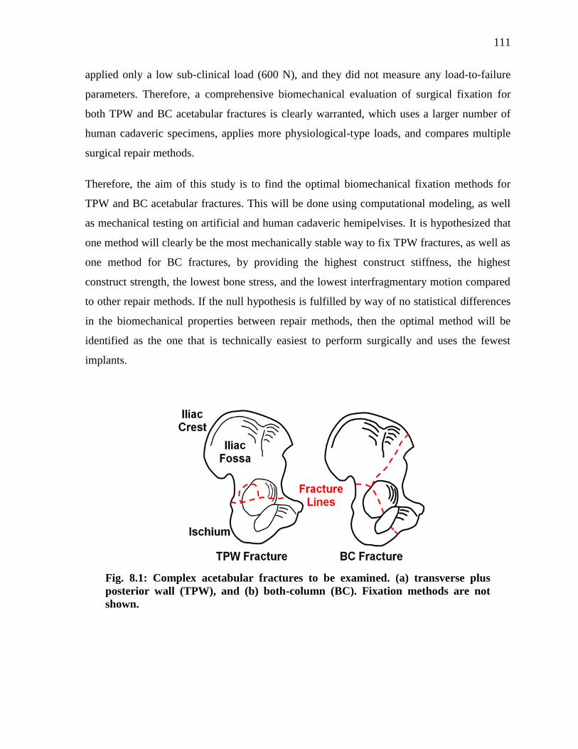
111

applied only a low sub-clinical load (600 N), and they did not measure any load-to-failure

parameters. Therefore, a comprehensive biomechanical evaluation of surgical fixation for

both TPW and BC acetabular fractures is clearly warranted, which uses a larger number of

human cadaveric specimens, applies more physiological-type loads, and compares multiple

surgical repair methods.

Therefore, the aim of this study is to find the optimal biomechanical fixation methods for

TPW and BC acetabular fractures. This will be done using computational modeling, as well

as mechanical testing on artificial and human cadaveric hemipelvises. It is hypothesized that

one method will clearly be the most mechanically stable way to fix TPW fractures, as well as

one method for BC fractures, by providing the highest construct stiffness, the highest

construct strength, the lowest bone stress, and the lowest interfragmentary motion compared

to other repair methods. If the null hypothesis is fulfilled by way of no statistical differences

in the biomechanical properties between repair methods, then the optimal method will be

identified as the one that is technically easiest to perform surgically and uses the fewest

implants.

Fig. 8.1: Complex acetabular fractures to be examined. (a) transverse plus

posterior wall (TPW), and (b) both-column (BC). Fixation methods are not

shown.

112

8.1.2 Importance of the Research Question

The goal of this study is to investigate the biomechanical stability of a series of surgical

methods for repairing TPW and BC acetabular fractures in order to determine an optimal

repair technique for each injury type. This will have several important consequences:

First, this study will be the only one in the literature to comprehensively address the

biomechanics of fixing TPW and BC acetabular fractures, which are the two most common

types of acetabular injuries.

Second, as a consequence of such evidence, orthopaedic surgeons will more easily identify

the best way to repair these fractures and adopt these methods into their practice based on

objective scientific evidence, rather than simply personal preference or subjective experience.

Third, choosing the best surgical repair method will also allow quicker and better fracture

union at the injury site, thus promoting healing, minimizing complications, and decreasing

the risk for re-operation.

Fourth, this will then allow patients to have earlier mobility and weight bearing shortly after

surgery, thereby facilitating a quicker recovery time, a regaining of their pre-injury functional

status, a return to their usual daily routines, and an increased quality of life.

Fifth, quicker recovery times result in shorter hospital stays, thus reducing overall healthcare

system financial costs.

Finally, this study will be the first step in validating the widely-used artificial hemipelvises

from Sawbones (Vashon, WA, USA) against human fresh-frozen cadaveric hemipelvises,

which are considered the “gold standard” for biomechanical testing. This will aid biomedical

engineers to improve the characteristics of these artificial hemipelvises and upgrade the

quality of future biomechanical investigations using these surrogate bones.

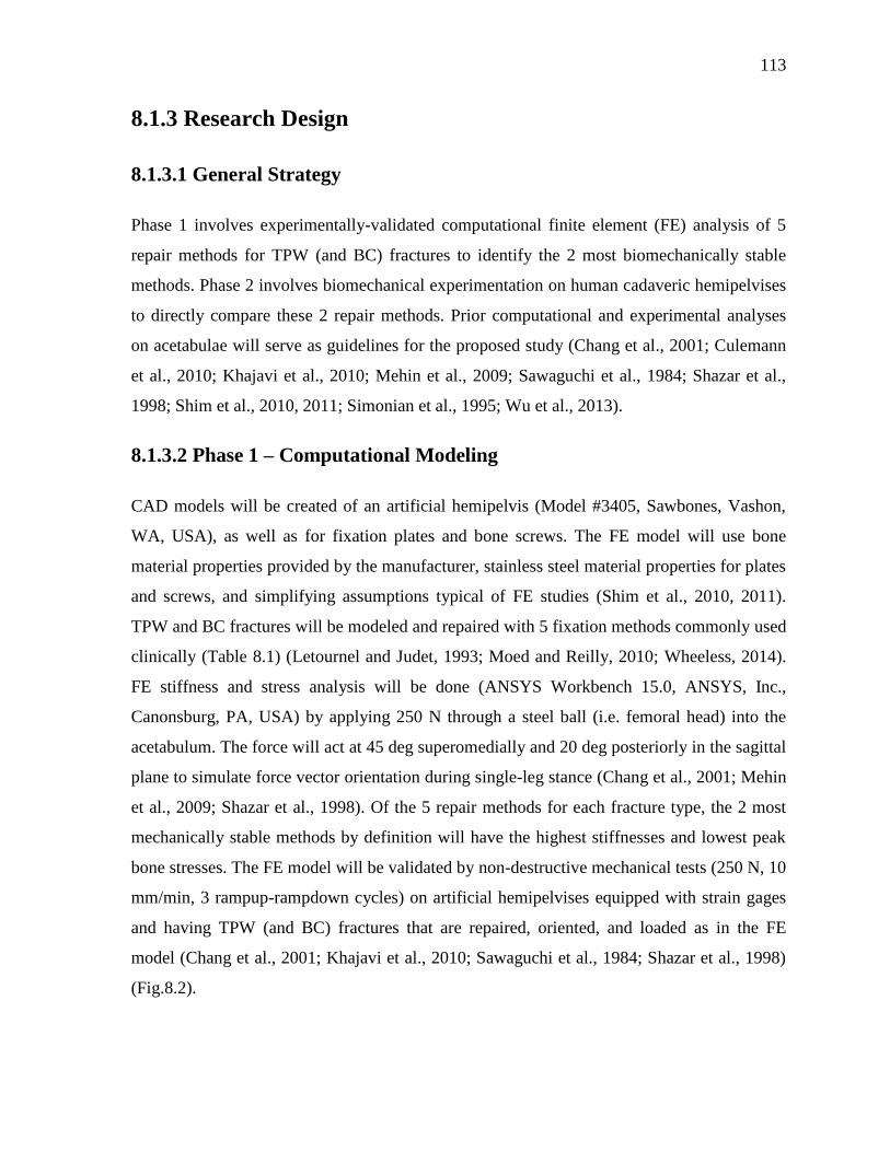
113

8.1.3 Research Design

8.1.3.1 General Strategy

Phase 1 involves experimentally-validated computational finite element (FE) analysis of 5

repair methods for TPW (and BC) fractures to identify the 2 most biomechanically stable

methods. Phase 2 involves biomechanical experimentation on human cadaveric hemipelvises

to directly compare these 2 repair methods. Prior computational and experimental analyses

on acetabulae will serve as guidelines for the proposed study (Chang et al., 2001; Culemann

et al., 2010; Khajavi et al., 2010; Mehin et al., 2009; Sawaguchi et al., 1984; Shazar et al.,

1998; Shim et al., 2010, 2011; Simonian et al., 1995; Wu et al., 2013).

8.1.3.2 Phase 1 – Computational Modeling

CAD models will be created of an artificial hemipelvis (Model #3405, Sawbones, Vashon,

WA, USA), as well as for fixation plates and bone screws. The FE model will use bone

material properties provided by the manufacturer, stainless steel material properties for plates

and screws, and simplifying assumptions typical of FE studies (Shim et al., 2010, 2011).

TPW and BC fractures will be modeled and repaired with 5 fixation methods commonly used

clinically (Table 8.1) (Letournel and Judet, 1993; Moed and Reilly, 2010; Wheeless, 2014).

FE stiffness and stress analysis will be done (ANSYS Workbench 15.0, ANSYS, Inc.,

Canonsburg, PA, USA) by applying 250 N through a steel ball (i.e. femoral head) into the

acetabulum. The force will act at 45 deg superomedially and 20 deg posteriorly in the sagittal

plane to simulate force vector orientation during single-leg stance (Chang et al., 2001; Mehin

et al., 2009; Shazar et al., 1998). Of the 5 repair methods for each fracture type, the 2 most

mechanically stable methods by definition will have the highest stiffnesses and lowest peak

bone stresses. The FE model will be validated by non-destructive mechanical tests (250 N, 10

mm/min, 3 rampup-rampdown cycles) on artificial hemipelvises equipped with strain gages

and having TPW (and BC) fractures that are repaired, oriented, and loaded as in the FE

model (Chang et al., 2001; Khajavi et al., 2010; Sawaguchi et al., 1984; Shazar et al., 1998)

(Fig.8.2).

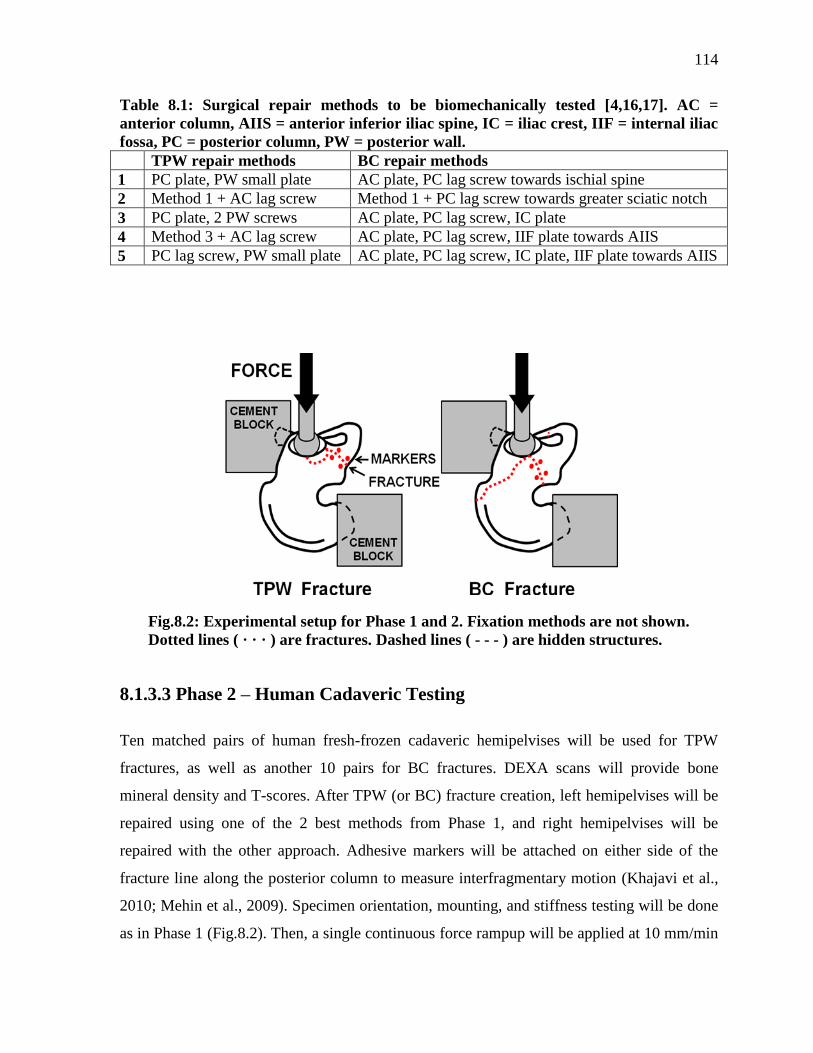
114

Table 8.1: Surgical repair methods to be biomechanically tested [4,16,17]. AC =

anterior column, AIIS = anterior inferior iliac spine, IC = iliac crest, IIF = internal iliac

fossa, PC = posterior column, PW = posterior wall.

TPW repair methods BC repair methods

1 PC plate, PW small plate AC plate, PC lag screw towards ischial spine

2 Method 1 + AC lag screw Method 1 + PC lag screw towards greater sciatic notch

3 PC plate, 2 PW screws AC plate, PC lag screw, IC plate

4 Method 3 + AC lag screw AC plate, PC lag screw, IIF plate towards AIIS

5 PC lag screw, PW small plate AC plate, PC lag screw, IC plate, IIF plate towards AIIS

Fig.8.2: Experimental setup for Phase 1 and 2. Fixation methods are not shown.

Dotted lines ( · · · ) are fractures. Dashed lines ( - - - ) are hidden structures.

8.1.3.3 Phase 2 – Human Cadaveric Testing

Ten matched pairs of human fresh-frozen cadaveric hemipelvises will be used for TPW

fractures, as well as another 10 pairs for BC fractures. DEXA scans will provide bone

mineral density and T-scores. After TPW (or BC) fracture creation, left hemipelvises will be

repaired using one of the 2 best methods from Phase 1, and right hemipelvises will be

repaired with the other approach. Adhesive markers will be attached on either side of the

fracture line along the posterior column to measure interfragmentary motion (Khajavi et al.,

2010; Mehin et al., 2009). Specimen orientation, mounting, and stiffness testing will be done

as in Phase 1 (Fig.8.2). Then, a single continuous force rampup will be applied at 10 mm/min

115

until structural collapse (Chang et al., 2001; Khajavi et al., 2010; Sawaguchi et al., 1984;

Shazar et al., 1998). Data analysis will be done for stiffness (i.e. slope of linear segment of

the force-vs-displacement graph), failure force (i.e. peak force), failure displacement (i.e.

displacement at peak force), failure energy (i.e. area under the curve up to the peak force),

and relative interfragmentary motion (i.e. from image analysis at 50 N, 250 N, and failure).

Statistical analysis will compare left-vs-right repair methods using paired student t tests with

significance at p<0.05. The optimal repair method for TPW (and BC) fractures will

statistically have the highest stiffness and failure parameters, and the lowest interfragmentary

motion. If there is no statistical difference, then the surgical procedure that uses fewer

implants and is technically easier to perform will be considered the optimal method.

116

References

Al-Qahtani, S., O’Connor, G., 1996. Acetabular fractures before and after the introduction of

seatbelt legislation. Can J Surg. 39, 317-20.

Aziz, M.S.R., Nicayenzi, B., Crookshank, M.C., Bougherara, H., Schemitsch, E.H., Zdero,

R., 2014a. Biomechanical Measurements of Stiffness and Strength for Five Types of Human

and Artificial Humeri. Journal of Biomechanical Engineering, 2014, 136(5), 051006-1-10

[Epub 2014 Mar 1].

Aziz, M.S.R., Nicayenzi, B., Crookshank, M.C., Bougherara, H., Schemitsch, E.H., Zdero,

R., 2014b. Biomechanical Measurements of Cortical Screw Purchase in Five Types of

Human and Artificial Humeri. Journal of the Mechanical Behavior of Biomedical Materials

30, 159-167.

Aziz M.S.R., Tsuji M.R.S., Nicayenzi B., Crookshank M.C., Bougherara H., Schemitsch

E.H., Zdero R., Biomechanical Measurements of Stopping and Stripping Torque during

Screw Insertion in Five Types of Human and Artificial Humeri, Proceedings of the

Institution of Mechanical Engineers (Part H): Journal of Engineering in Medicine, 2014,1-10.

Bellabarba, C., Berger, R.A., Bentley, C.D., et al., 2001. Cementless acetabular

reconstruction after acetabular fracture. J Bone Joint Surg Am. 83, 868–876.

Bergmann, G., Graichen, F., Rohlmann, A., 1993. Hip joint loading during walking and

running, measured in two patients. J Biomech. 26, 969–990.

Bitsakos, C., Kerner, J., Fisher, I., Amis, A.A., 2005. The effect of muscle loading on the

simulation of bone remodeling in the proximal femur. Journal of Biomechanics 38, 133–139.

Blum, J., Beyermann, K., Ritter, G., 1991. Incidence of acetabular fractures before and after

introduction of compulsory seatbelt fastening. Unfallchirurgie 17, 274-9 (in German).

Boraiah, S., Ragsdale, M., Achor, T., Zelicof, S., Asprinio, D.E., 2009. Open Reduction

Internal Fixation and Primary Total Hip Arthroplasty of Selected Acetabular Fractures. J

Orthop Trauma 23, 243–248.

Bougherara, H., Zdero, R., Miric, M., Shah, S., Hardisty, M., Zalzal, P., Schemitsch E.H.,

2009. The biomechanics of the T2 femoral nailing system: a comparison of synthetic femurs

with finite element analysis. Proc. IMechE, Part H: J. Engineering in Medicine 223, 303-314.

Bougherara, H., Bureau, M.N., Yahia, L., 2010a. Bone remodeling in a new biomimetic

polymer-composite hip stem. Journal of Biomedial Materials Research Part A 92 (1), 164–

174.

Bougherara, H., Zdero, R., Shah, S., Miric, M., Papini, M., Zalzal, P., Schemitsch E.H.,

2010b. A biomechanical assessment of modular and monoblock revision hip implants using

117

FE analysis and strain gage measurements. Journal of Orthopaedic Surgery and Research 5,

34.

Bougherara, H., Rahim, E., Shah, S., Dubov, A., Schemitsch, E.H., Zdero, R., 2011a. A

preliminary biomechanical assessment of a polymer composite hip implant using an infrared

thermography technique validated by strain gage measurements. Journal of Biomechanical

Engineering 133 (7), 074503 1–6.

Bougherara, H., Zdero, R., Dubov, A., Shah, S., Khurshid, S., Schemitsch, E.H., 2011b. A

preliminary biomechanical study of a novel carbon-fibre hip implant versus standard metallic

hip implants. Medical Engineering and Physics 33, 121–128 [Epub 2010 Oct 15].

Brockstedt, H., Kassem, M., Eriksen, E.F., Mosekilde, L., Melsen, F., 1993. Age- and sex-

related changes in iliac cortical bone mass and remodeling. Bone, 14, 681-691.

Carroll, E.A., Huber, F.G., Goldman, A.T., Virkus, W.W., Pagenkopf, E., Lorich, D.G.,

Helfet, D.L., 2010. Treatment of Acetabular Fractures in an Older Population. J Orthop

Trauma 24, 637–644.

Chang, J.K., Gill, S.S., Zura, R.D., Krause, W.R., Wang, G.J., 2001. Comparative strength of

three methods of fixation of transverse acetabular fractures. Clinical Orthop Relat Res. 392,

433-441.

Court-Brown, C.M., Aitken, S.A., Forward, D., O’Toole, R.V., 2006. The epidemiology of

fractures, (chapter 3). In: Bucholz, R.W., Heckman, J.D., Court-Brown, C.M., Tornetta, P.

(eds.), Rockwood and Green's Fractures in Adults: Volume 1, Lippincott, pp.53-83.

Court-Brown, C.M., Aitken, S.A., Forward, D., O’Toole, R.V., 2010. The epidemiology of

fractures, (chapter 3). In: Bucholz, R.W., Heckman, J.D., Court-Brown, C.M., Tornetta, P.

(eds.), Rockwood and Green's Fractures in Adults: Volume 1, Lippincott, pp.53-83.

Cristofolini, L., Viceconti, M., Cappello, A., Toni, A., 1996. Mechanical validation of whole

bone composite femur models. J. Biomech. 29 (4), 525–535.

Culemann, U., Holstein, J.H., Köhler, D., Tzioupis, C.C., Pizanis, A., Tosounidis, G.,

Burkhardt, M., Pohlemann, T., 2010. Different stabilisation techniques for typical acetabular

fractures in the elderly--a biomechanical assessment. Injury, 41 (4), 405-410.

Davies, J.E., 2003. Understanding Peri-implant endosseous healing. Re-issued from: Journal

of Dental Education 67 (8).

Davis, E.T., Olsen, M., Zdero, R., Waddell, J.P., Schemitsch, E.H., 2008. Femoral neck

fracture following hip resurfacing: The effect of alignment of the femoral component. J Bone

Joint Surg Br. 90 (11), 1522-1527.

Dennis, M.G., Simon, J.A., Kummer, F.J., Koval, K.J., DiCesare, P.E., 2000. Fixation of

periprosthetic femoral shaft fractures occurring at the tip of the stem: a biomechanical study

of 5 techniques. J. Arthroplasty 15 (4), 523–528.

118

Dennis, M.G., Simon, J.A., Kummer, F.J., Koval, K.J., DiCesare, P.E., 2001. Fixation of

periprosthetic femoral shaft fractures: a biomechanical comparison of two techniques. J.

Orthop. Trauma 15 (3), 177–180.

Dubov, A., Kim, S.Y.R., Shah, S., Schemitsch, E.H., Zdero, R., Bougherara, H., 2011. The

biomechanics of plate repair of periprosthetic femur fractures near the tip of a total hip

implant: The effect of cable-screw position. Proc. IMechE, Part H: J. Engineering in

Medicine 225, 857-865.

Ebrahimi, H., Rabinovich, M., Vuleta, V., Zalcman, D., Shah, S., Dubov, A., Roy, K.,

Siddiqui, F.S. Schemitsch, E.H., Bougherara, H., Zdero, R., 2012. Biomechanical Properties

of an Intact, Injured, Repaired, and Healed Femur: An Experimental and Computational

Study. J Mechanical Behavior of Biomedical Materials 16, 121-35.

Ferguson, T.A., Patel, R., Bhandari, M., Matta, J.M., 2010. Fractures of the acetabulum in

patients aged 60 years and older; An epidemiological and radiological study. The Journal of

Bone and Joint Surgery, 92-B(2), 250-7.

Foldes, J., Parfitt, A.M., Shih, M.S., Rao, D.S., Kleerekoper, M., 1991. Structural and

geometric changes in iliac bone: Relationship to normal aging and osteoporosis. J Bone and

Mineral research, 6 (7),759-766.

Fulkerson, E., Koval, K., Preston, C.F., Iesaka, K., Kummer, F.J., Egol, K.A, 2006. Fixation

of periprosthetic femoral shaft fractures associated with cemented femoral stems: a

biomechanical comparison of locked plating and conventional cable plates. J. Orthop.

Trauma 20 (2), 89–93.

Gilliland, J.M., Anderson, L.A., Henninger, H.B., Kubiak, E.N., Peters, C.L., 2013.

Biomechanical analysis of acetabular revision constructs; Is pelvic discontinuity best treated

with bicolumnar or traditional unicolumnar fixation? The Journal of Arthroplasty 28 (1),

178-186.

Gray, H., 2000. Anatomy of the human body. Philadelphia: Lea & Febiger, 1918;

Bartleby.com, www.bartleby.com/107/.

Grazier, K.L., Holbrook, T.L., Kelsey, J.L., Stauffer, R.N., 1984. The frequency of

occurrence, impact, and cost of selected musculoskeletal conditions in the United States.

Chicago: American Academy of Orthopaedic Science 24-72.

Gross, A.E., Allan, D.G., Catre, M., et al., 1993. Bone grafts in hip replacement surgery. The

pelvic side. Orthop Clin North Am. 24, 679–695.

Hak, D.J., Toker, S., Yi, C., Toreson, J., 2010. The Infleuence of Fracture Fixation

Biomechanics on Fracture Healing. J. of Trauma Update 33 (10), 752-5.

Harris, W.H., 1996. Traumatic arthritis of the hip. J Bone Joint Surg Am. 51, 737–755.

Helfet, D.L., Borrelli, J. Jr., DiPasquale, T., Sanders, R., 1992. Stabilization of acetabular

119

fractures in elderly patients. J Bone Joint Surg [Am] 74-A, 753-65.

Herscovici, D., Lindvall, E., Bolhofner, B., Scaduto, J.M., 2010. The Combined Hip

Procedure: Open Reduction Internal Fixation Combined With Total Hip Arthroplasty for the

Management of Acetabular Fractures in the Elderly. J. Orthop. Trauma 24 (5), 291-6.

Hessmann, M.H., Nijs, S., Rommens, P.M., 2002. Acetabular fractures in the elderly. Results

of a sophisticated treatment concept. Unfallchirurgie 105, 893–900.

JA Goulet, J.A., Rouleau, J.P., Mason D.J., Goldstein S.A., 1994. Comminuted fractures of

the posterior wall of the acetabulum. A biomechanical evaluation of fixation methods. J Bone

Joint Surg Am. 76 (10), 1457-63.

Jeanotte, L., Moore, M.J., 2007. The State of Aging and Health in America. The Merck

Company Foundation. Whitehouse Station, NJ, 2007. http://www.cdc.gov/Aging/pdf/

saha_2007.pdf (date last accessed 29 June 2014).

Jimenez, M.L., Tile, M., Schenk, R.S., 1997. Total hip replacement after acetabular fracture.

Orthop. Clin. North America 28, 435-446.

Joly, J.M., Mears, D.C., 1993. The role of total hip arthroplasty in acetabular fracture

management. Operative Techniques Orthop. 3, 80–102.

Kang, C.S., Min, B.W., 2002. Cable fixation in displaced fractures of the acetabulum; 21

patients followed for 2-8 years. Acta Orrbop Scand 73 (6), 619-624.

Khajavi, K., Lee, A.T., Lindsey, D.P., Leucht, P., Bellino, M.J., Giori, N.J., 2010. Single

column locking plate fixation is inadequate in two column acetabular fractures. A

biomechanical analysis. Journal of Orthopaedic Surgery and Research 5, 30.

Knight, R.A., Smith, H., Central fractures of the acetabulum. J. Bone and Joint Surg. 40-A,

1-16.

Kreder, H.J., Rozen, N., Borkhoff, C.M., et al., 2006. Determinants of functional outcome

after simple and complex acetabular fractures involving the posterior wall. J Bone Joint Surg

Br. 88, 776–782.

Laird, A., Keating, J.F., 2005. Acetabular fractures, A 16-year prospective epidemiological

study. Journal of Bone and Joint Surgery (Br), 87, 969-973.

Lead wire attachment technique: http://www.vishaypg.com/docs/11084/tt604.pdf [Last

accessed: 29 June 2014].

Letournel, E., Judet, R., 1981. Fractures of the acetabulum. Springer-Verlag, Berlin

Heidelberg, New York.

Letournel, E., Judet, R., 1993. Clinical and radiological results of operation within three

weeks of injury. Fractures of the Acetabulum. Ed 2. Berlin, Springer-Verlag 565–581.

120

Letournel, E., Judet, R., 1993. Fractures of the Acetabulum, edited by R. A. Elson. New

York, Springer.

Lever, J.P., Zdero, R., Nousiainen, M.T., Waddell, J.P., Schemitsch, E.H., 2010. The

biomechanical analysis of three plating fixation systems for periprosthetic femoral fracture

near the tip of a total hip arthroplasty. J. Orthop. Surg. Res. 5:45.

Levine, M.A., 1943. A treatment of central fractures of the acetabulum. J. Bone and Joint

Surg. 25, 902-906.

Liu, X., Xu, S., Zhang, C., Fu, Q., Wang, P., 2010. Biomechanical study of posterior wall

acetabular fracture fixation using acetabular tridimensional memory alloy-fixation system.

Clinical Biomechanics 25, 312–317.

Lonner, J.H., Koval, K.J., 1995. Polytrauma in the elderly. Clin. Orthop. 318, 136-43.

Marsh, J.L., et al., 2007. Fracture and dislocation classification compendium – 2007:

Orthopaedic Trauma Association classification, database and outcomes committee. Journal

of Orthopaedic Trauma, 21 (10), S59-S67.

Matta, J.M., 1996. Fractures of the acetabulum. Accuracy of reduction and clinical results in

patients managed operatively within three weeks after the injury. J Bone Joint Surg Am. 78,

1632–1645.

Matta, J.M., Anderson, L.M., Epstein, H.C., et al., 1986. Fractures of the acetabulum. A

retrospective analysis. Clin Orthop Relat Res. 205, 230–240.

Matta, J.M., Mehne, D.K., Roffi, R., 1986. Fractures of the acetabulum. Early results of a

prospective study. Clin Orthop Relat Res 241—50.

Matta, J.M., Mernt, P., 1988. Displaced acetabular fractures. Clin Orthop Relat Res. 230, 83–

97.

De Ridder, V.A., De Lange, S., Kingma, L., et al., 1994. Results of 75 consecutive patients

with acetabular fractures. Clin Orthop Relat Res. 305, 53–57.

Mayo, K.A., 1994. Open reduction and internal fixation of fractures of the acetabulum.

Results in 163 fractures. Clin Orthop Relat Res. 305, 31–7.

McConnell, A., Zdero, R., Syed, K., Peskun, C., Schemitsch, E.H., 2008. The Biomechanics

of Ipsilateral Intertrochanteric and Femoral Shaft Fractures: A Comparison of 5 Fracture

Fixation Techniques, Journal of Orthopaedic Trauma, 22 (8), 517-524.

Mears, D.C., 1999. Surgical treatment of acetabular fractures in elderly patients with

osteoporotic bone. J. Am. Acad. Orthop. Surg.7, 128-41.

Mears, D.C., Rubash, H.E., 1986. Approaches to the Pelvic Ring and Acetabulum. Pelvic and

Acetabular Fractures. Thorofare, NJ, Slack Inc 215–249.

121

Mears, D.C., Shirahama, M., 1998. Stabilization of an acute acetabular fracture with cables

for acute total hip arthroplasty. The Journal of Arthroplasty 13 (1), 104-7.

Mears, D.C., Velyvis, J.H., 2000. Primary Total Hip Arthroplasty After Acetabular Fracture.

An Instructional Course Lecture, American Academy of Orthopaedic Surgeons 50, Journal of

Bone and Joint Surgery 82-A, 9, 1328-53.

Mears, D.C., Velyvis, J.H., 2002. Acute total hip arthroplasty for selected displaced

acetabular fractures: two to twelve-year results. J Bone Joint Surg [Am] 84-A, 1-9.

Mears, D.C., Velyvis, J.H., Chang, C.P., 2003. Displaced acetabular fractures managed

operatively: indicators of outcome. Clin Orthop 407, 173-86.

Mears, D.C., Ward, A.J., 1996. Late results of total hip arthroplasty to manage posttraumatic

arthritis of acetabular fractures. Fractures of the pelvis and the acetabulum. Presented at the

Third International Consensus; Pittsburgh, PA.

Mehin, R., Jones, B., Zhu, Q., Broekhuyse, H., 2009. A biomechanical study of conventional

acetabular internal fracture fixation versus locking plate fixation. Canadian Journal of

Surgery 52 (3), 221-228.

Moed, B.R., Reilly, M.C., 2010. Acetabulum fractures, In: Bucholz RW, Heckman JD,

Tornetta P, III, eds, Rockwood and Green's fractures in adults, 7th

edition, Philadelphia:

Wolters Kluwer Health/Lippincott Williams & Wilkins, chapter 45, 1463-1523.

Moed, B.R., Wilson-Carr, S.E,, Watson, J.T., 2002. Results of operative treatment of

fractures of the posterior wall of the acetabulum. J Bone Joint Surg Am. 84, 752–8.

Mouhsine, E., Garofalo, R., Borens, O., Blanc, C.H., Wettstein, M., Leyvraz, P.F., 2004.

Cable Fixation and Early Total Hip Arthroplasty in the Treatment of Acetabular Fractures in

Elderly Patients. The Journal of Arthroplasty 19 (3), 344-8.

Mouhsine, E., Garofalo, R., Borens, O., Fischer, J.F., Crevoisier, X., Pelet, S., Blanc, C.H.,

Leyvraz, P.F., 2002. Acute total hip arthroplasty for acetabular fractures in the elderly; 11

patients followed for 2 years. Acta Orthop Scand 73 (6), 615-8.

Murphy, D., Kaliszer, M., Rice, J., et al., 2003. Outcome after acetabular fracture: prognostic

factors and their inter-relationships. Injury 34, 512–7.

Olson, S.A., Bay, B.K., Chapman, M.W., Sharkey, N.A., 1995. Biomechanical consequences

of fracture and repair of the posterior wall of the acetabulum. J Bone Joint Surg Am. 77 (8),

1184-92.

Olson, S.A., Bay, B.K., Pollak, A.N., Sharkey, N.A., Lee, T., 1996. The Effect of Variable

Size Posterior Wall Acetabular Fractures on Contact Characteristics of the Hip Joint. Journal

of Orthopaedic Trauma 10 (6), 395-402.

122

Pagenkopf, E., Grose, A., Partal, G., Helfet, D.L., 2006. Acetabular Fractures in the Elderly:

Treatment Recommendations. HSSJ 2, 161–171.

Pal, B., Gupta, S., New, A.M.R., 2010. Influence of the change in stem length on the load

transfer and bone remodelling for a cemented resurfaced femur. J Biomech. 43 (15), 2908-

2914.

Papini, M., Zdero, R., Schemitsch, E.H., Zalzal, P., 2007. The biomechanics of human

femurs in axial and torsional loading: Comparison of finite element analysis, human

cadaveric femurs, and synthetic femurs. J Biomech Eng. 129 (1), 12-19.

Peters, C.L., Bachus, K.N., Davitt, J.S., 2003. Fixation of periprosthetic femur fractures: a

biomechanical analysis comparing cortical strut allograftvplates and conventional metal

plates. Orthopedics 26 (7), 695–699.

Romness, D.W., Lewallen, D.G., 1990. Total hip arthroplasty after fracture of the

acetabulum. Long-term results. J. Bone and Joint Surg., 72-B(S): 761-764.

Rosette strain gauge: http://www.vishaypg.com/docs/11124/062ur.pdf [Last accessed: 29

June, 2014].

Routt, M.L.C., Jr., Swiontkowski, M.F., 1990. Operative treatment of complex acetabular

fractures. Combined anterior and posterior approaches during the same procedure. J Bone

Joint Surg Am. 72, 897–904.

Rowe, C.R., Lowell, J.D., 1961. Prognosis of fractures of the acetabulum. J Bone Joint Surg

43A, 30–59.

Ruesch, P.D., Holdener, H., Ciaratmitaro, M., et al., 1994. A prospective study of surgically

treated acetabular fractures. Clin Orthop Relat Res. 305, 38–46.

Sarkar, M.R., Wachter, N., Kinzl, L., Bischoff, M., 2004. Joint Replacement for Acetabular

Fractures. Acute Total Hip Replacement for Displaced Acetabular Fractures in Older

Patients. Eur J Trau ma. 30, 296–304.

Sawaguchi, T., Brown, T.D., Rubash, H.E., Mears, D.C., 1984. Stability of acetabular

fractures after internal fixation; A cadaveric study. Acta Orthopaedica Scandinavica 55, 601-

5.

Schmotzer, H., Tchejeyan, G.H., Dall, D.M., 1996. Surgical management of intra- and

postoperative fractures of the femur about the tip of the stem in total hip arthroplasty. J.

Arthroplasty 11 (6), 709–717.

Shah, S., Kim, S.Y.R., Dubov, A., Schemitsch, E.H., Bougherara, H., Zdero, R., 2011. The

biomechanics of plate fixation of periprosthetic femoral fractures near the tip of a total hip

implant: cables, screws, or both? Proc. IMechE, Part H: J. Engineering in Medicine 225, 845-

856.

123

Shazar, N., Brumback, R.J., Novak, V.P., Belkoff, S.M., 1998. Biomechanical evaluation of

transverse acetabular fracture fixation, Clinical Orthopaedics and Related Research 352, 215-

222.

Shim, V., Böhme, J., Vaitl, P., Klima, S., Josten, C., Anderson, I., 2010. Finite element

analysis of acetabular fractures--development and validation with a synthetic pelvis. Journal

of Biomechanics 43 (8), 1635-1639.

Shim, V.B., Böshme, J., Vaitl, P., Josten, C., Anderson, I.A., 2011. An efficient and accurate

prediction of the stability of percutaneous fixation of acetabular fractures with finite element

simulation. Journal of Biomechanical Engineering 133 (9), 094501.

Simonian, P.T., Routt, M.L., Jr., Harrington, R.M., Tencer, A.F., 1995. The acetabular T-

type fracture. A biomechanical evaluation of internal fixation. Clinical Orthop Relat Res 314,

234-240.

Strain gauge surface preparation: http://www.vishaypg.com/docs/11129/11129_b1.pdf [Last

accessed: 29 June 2014].

Stevens, S.S., Irish, A.J., Vachtsevanos, J.G., Csongradi, J., Beaupre, G.S., 1995. A

biomechanical study of three wiring techniques for cerclage-plating. Journal of Orthopaedic

Trauma 9 (5), 381–387.

Stolk, J., Verdonschot, N., Huiskes, R., 2001. Hip-joint and abductor-muscle forces

adequately represent in vivo loading of a cemented total hip reconstruction. Journal of

Biomechanics 34, 917–926.

Talbot, M., Zdero, R., Schemitsch, E.H., 2008a. Cyclic loading of periprosthetic fracture

fixation constructs. J. Trauma 64 (5), 1308–1312.

Talbot, M., Zdero, R., Garneau, D., Cole, P.A., Schemitsch, E.H., 2008b. Fixation of long

bone segmental defects: a biomechanical study. Injury 39 (2), 181–186.

Three-wire quarter-bridge circuit: http://www.vishaypg.com/docs/11092/tt612.pdf [Last

accessed: 29 June 2014].

Tidermark, J., Blomfeldt, R., Ponzer, S., Söderqvist, A., Törnkvist, H., 2003. Primary Total

Hip Arthroplasty with a Burch-Schneider Antiprotrusion Cage and Autologous Bone

Grafting for Acetabular Fractures in Elderly Patients. Journal of Orthopaedic Trauma 17 (3),

193-7.

Tile, M., 1994. Introduction to Acetabular Fractures. Fractures of the Pelvis and Acetabulum.

Ed 2. Baltimore, Williams and Wilkins 249–248.

Tuncer, M., Hansen, U.N., Amis, A.A., 2014. Prediction of structural failure of tibial bone

models under physiological loads: Effect of CT density-modulus relationships. Med Eng

Phys. doi: 10.1016/j.medengphy.2014.04.006. [Epub ahead of print].

124

Vanderschot, P., 2007. Treatment options of pelvic and acetabular fractures in patients with

osteoporotic bone. Injury, Int. J. Care Injured 38, 497—508.

Vedi, S., Kaptoge, S., Compston, J.E., 2011. Age-related changes in iliac crest cortical width

and porosity: a histomorphometric study. J Anat., 218, 510-516.

Weber, M., Berry, D.J., Harmsen, W.S., 1998. Total hip arthroplasty after operative

treatment of an acetabular fracture. J Bone Joint Surg Am. 80, 1295–1305.

Wheeless, C.R., III, Wheeless’ Textbook of Orthopaedics. Last accessed on 29 June 2014,

http://www.wheelessonline.com/ortho/fractures_of_the_acetabulum

Wilson, D., Frei, H., Masri, B.A., Oxland, T.R., Duncan, C.P., 2005. A biomechanical study

comparing cortical onlay allograft struts and plates in the treatment of periprosthetic femoral

fractures. Clin. Biomech. (Bristol, Avon) 20 (1), 70–76.

Witte, H., Eckstein, F., Recknagel, S., 1997. A calculation of the forces acting on the human

acetabulum during walking, based on in vivo force measurements, kinematic analysis and

morphometry. Acta Anat. 160, 269-280.

Wolinsky, P.R., Davison, B.L., Shyr, Y., et al., 1996. Predictors of total hip arthroplasty in

patients following open reduction and internal fixation of acetabular fractures. Proceedings of

the 12th Annual Orthopaedic Trauma Association Meeting 9, 29. Abstract.

Wright, R., Barrett, K., Christie, M.J., et al., 1994. Acetabular fractures. Long-term follow-up

of open reduction and internal fixation. J Orthop Trauma 8, 397–403.

Wu, Y.D., Cai, X.H., Liu, X.M., Zhang, H.X., 2013. Biomechanical analysis of the

acetabular buttress-plate: Are complex acetabular fractures in the quadrilateral area stable

after treatment with anterior construct plate-1/3 tube buttress plate fixation? Clinics, 68 (7),

1028-1033.

Yuntong, Z., Yang, T., P, W., Xue, Z., Shuogui, X., Chuncai, Z., 2013. Biomechanical

Comparison of Different Stabilization Constructs for Unstable Posterior Wall Fractures of

Acetabulum. A Cadaveric Study. PLoS ONE 8 (12), e82993.

Zdero, R., Olsen, M., Bougherara, H., Schemitsch, E.H., 2008a. Cancellous bone screw

purchase: a comparison of synthetic femurs, human femurs, and finite element analysis. Proc

IMechE, Part H: J. Eng. Med. 222 (H8), 1175–1183.

Zdero, R., Walker, R., Waddell, J.P., Schemitsch, E.H., 2008b. Biomechanical evaluation of

periprosthetic femoral fracture fixation. J. Bone Joint Surg. Am. 90 (5), 1068–1077.

Zdero, R., Elfallah, K., Olsen, M., Schemitsch, E.H., 2009. Cortical screw purchase in

synthetic and human femurs. J. Biomech. Eng. 131 (9), 094503-1-7.