Biomechanical Modeling of Soft Tissue and Facial ... · Soft Tissue and Facial Expressions for...
145
Biomechanical Modeling of Soft Tissue and Facial Expressions for Craniofacial Surgery Planning Dissertation von Evgeny Gladilin eingereicht am Fachbereich Mathematik und Informatik der Freien Universit¨ at Berlin im Oktober 2002
Transcript of Biomechanical Modeling of Soft Tissue and Facial ... · Soft Tissue and Facial Expressions for...

Biomechanical Modeling ofSoft Tissue and Facial Expressionsfor Craniofacial Surgery Planning
Dissertation vonEvgeny Gladilin
eingereicht amFachbereich Mathematik und Informatik
der Freien Universitat Berlin
im Oktober 2002

Betreuer: Prof. Dr. Dr. h.c. Peter DeuflhardKonrad-Zuse-Zentrum fur Informationstechnik Berlin (ZIB)Takustr. 714195 Berlin
Gutachter: Prof. Dr. Dr. h.c. Peter DeuflhardProf. Dr. Markus Gross
Datum der Disputation: 11.06.2003
Acknowledgments
First, I would like to thank Peter Deuflhard for inviting me to Zuse-Institute-Berlin (ZIB) to participate on the computer assisted surgery (CAS) project thathas been originated with his vision of the realistic modeling of the human face onthe basis of consistent numerical methods. I am indebted to him for his guidanceof my work and for giving me the freedom to go my own, often only intuitivelyapproachable ways to achieve research goals.
Such multi-disciplinary work would be unimaginable without the cooperationwith many people directly or indirectly contributing and supporting it. I thankmy colleague within the CAS-project, Stefan Zachow, for providing geometri-cal models of human anatomy, which essentially helped this work to become anapplication-oriented effort. I thank Martin Seebass for discussions around the top-ics of geometrical modeling and visualization. I am grateful to Hans-ChristianHege for his personal engagement and many-sided support of this fascinatingproject from its very beginning on. My thanks go to my colleagues from Sci-entific Computing Department of ZIB and Free University of Berlin: Bodo Erd-mann, Jens Lang, Rainer Roitzsch and Rolf Krause for their assistance and manypractical advices w.r.t. the structural mechanics modeling and the finite elementprogramming, especially at the beginning of this work. I would like to expressmy great thanks to Martin Weiser for many helpful discussions across the field ofnumerical analysis. Finally, I thank my family and my friends for supporting methroughout the last three years.
Tomographic data used in this work were kindly provided by our clinicalpartners, Hans-Florian Zeilhofer and Robert Sader from the clinic for cranio-maxillofacial surgery, Technical University Munich (Klinik und Poliklinik furMKG-Chirurgie der TU Munchen, Klinikum rechts der Isar).


Contents
1 Introduction 11.1 Motivation . . . . . . . . . . . . . . . . . . . . . . . . . . . . . . 11.2 Problem Description . . . . . . . . . . . . . . . . . . . . . . . . 21.3 Contributions . . . . . . . . . . . . . . . . . . . . . . . . . . . . 51.4 Overview . . . . . . . . . . . . . . . . . . . . . . . . . . . . . . 6
2 State of the Art 72.1 Deformable Modeling . . . . . . . . . . . . . . . . . . . . . . . . 72.2 Non-physical Modeling . . . . . . . . . . . . . . . . . . . . . . . 82.3 Physical Modeling . . . . . . . . . . . . . . . . . . . . . . . . . 9
3 Background Knowledge 163.1 Facial Tissue. Structure and Properties . . . . . . . . . . . . . . . 163.2 Basics of Continuum Mechanics . . . . . . . . . . . . . . . . . . 243.3 Finite Element Method . . . . . . . . . . . . . . . . . . . . . . . 34
4 Geometrical Modeling 514.1 Image Segmentation . . . . . . . . . . . . . . . . . . . . . . . . 514.2 Mesh Generation . . . . . . . . . . . . . . . . . . . . . . . . . . 534.3 Mesh Quality Control . . . . . . . . . . . . . . . . . . . . . . . . 554.4 Derivation of Boundary Conditions . . . . . . . . . . . . . . . . . 58
5 Numerical Model 605.1 Simplified Numerical Model of Facial Tissue . . . . . . . . . . . 605.2 Sensitivity Analysis and Parameter Estimation . . . . . . . . . . . 615.3 Details of Implementation . . . . . . . . . . . . . . . . . . . . . 65
6 Static Soft Tissue Prediction 696.1 Experiments with Artificial Objects . . . . . . . . . . . . . . . . 696.2 Soft Tissue Prediction in the CAS Planning . . . . . . . . . . . . 76
i

7 Individual Facial Expressions 927.1 Facial Animation . . . . . . . . . . . . . . . . . . . . . . . . . . 937.2 Anatomy and Physiology of Muscles . . . . . . . . . . . . . . . . 957.3 Biomechanical Models of Contracting Muscles . . . . . . . . . . 987.4 Virtual Fibers . . . . . . . . . . . . . . . . . . . . . . . . . . . . 1017.5 Experimental Results . . . . . . . . . . . . . . . . . . . . . . . . 103
Conclusion 121
Appendices 124
A Notation 125
B Fundamental Solution of Linear Elasticity 128
ii

An intellect which at any given moment knew all the forces that animate Na-ture and the mutual positions of the beings that comprise it, if this intellect werevast enough to submit its data to analysis, could condense into a single formulathe movement of the greatest bodies of the universe and that of the lightest atom:for such an intellect nothing could be uncertain; and the future just like the pastwould be present before our eyes.
P. S. Laplace (1749-1827), Philosophical Essay on Probabilities [78].


Chapter 1
Introduction
1.1 Motivation
The advances in medical imaging beginning from the discovery of X-rays formore than 100 years ago, open nowadays new perspectives for the improvementof the computer assisted surgery planning (CASP). Meanwhile, modern medicalimaging techniques, such as computer tomography (CT) and magnetic resonanceimaging (MRI), are widely-used for diagnostic and visualization purposes enablethe derivation of useful 3D models of human anatomy. 3D body models providethe information on the geometrical disposition of different anatomical structuresonly. However, the main goal of computer assisted surgery (CAS) is to simulatephysical interactions with virtual bodies. In particular, the realistic simulation ofsoft tissue deformations under the impact of external forces is of crucial impor-tance. It is the task of the biomechanical modeling to assign reliable physicalproperties to virtual anatomical structures in order to make them interact accord-ing to underlying physical laws. The nearer a physical model approaches theproperties of a living tissue the more realistic the simulation results can be ob-tained. This predication is the central paradigm of the physically based soft tissuemodeling.
In cranio-, dento-maxillofacial surgery, there is a great demand for efficientcomputer assisted methods, which could enable flexible, accurate and robust sim-ulations of surgical interventions on virtual patients, including the realistic predic-tion of their postoperative appearance. The computer assisted surgical planninghas many advantages in comparison with conventional planning systems. Oncethe virtual model of a patient is generated, various case scenarios of the surgicalimpact and their outcomes can be extensively studied. Better preparation, shorteroperation time, lower costs are the immediate benefits. Since the improvement of
1

2 Chapter 1. Introduction
the patient’s aesthetics is one of the main aims in craniofacial surgery, the realisticprediction of the patient’s postoperative appearance is an important feature of theplanning system giving the surgeon unique feedback already during the planningstage.
In addition to the static soft tissue prediction, the estimation of individual fa-cial emotion expressions is another important criterion for the prediction of post-operative results as well as for patient compliance. In certain cases, as for instancefacial paralysis treatment, the estimation of single muscle actions is even of pri-mary interest for the surgical planning.
1.2 Problem Description
The topic of soft tissue modeling has been the subject of intensive investigationsof many research groups within the last three decades. Because of the complexityof soft tissue behavior and diverse types of application fields, a wide spectrumof approaches has been developed. In Table 1.1, a brief overview of the rangeof problems arising within the scope of soft tissue modeling is given. From thisoverview, it is already evident that there is no general modeling approach, whichcould cover the whole spectrum of soft tissue biomechanics and serve for all vari-ous medical applications. In fact, modeling complex living systems implies manyintrinsic controversies. For instance, the requirement of the increasing realismof the simulation is often associated with the decrease of the efficiency and/orthe robustness of a more sophisticated modeling approach. The real-time perfor-mance can hardly be realized on low-cost hardware platforms, etc. Consequently,the way of simplification of the original complex problem is usually preferred.Which particular aspect or property of a complex soft tissue model has to be con-sidered, and, which can be neglected, essentially depends on the order of priorityof the concrete characteristic of the given problem.
The goal of the present thesis is the development of a biomechanical model offacial tissue tailored to the particular needs of the craniofacial surgery planning,
• the static soft tissue prediction and
• the estimation of individual facial emotion expressions.
Such problem definition has already certain important consequences for the choiceof an adequate modeling approach, which in turn paves the way for some substan-tial simplifications. In the following, we formulate some important statements,which give a more detailed description of the problem to be studied in the presentwork and range the preliminary scope of further investigations.

1.2. Problem Description 3
Table 1.1: Soft tissue modeling. Range of problems
Tissue Type Field of Application
brain-liquor neurosurgeryparenchymal organs inner surgerycardio-vascular system cardiologyconnective tissue sport-medicinemusculoskeleton biokinematicsskin, fat, muscles craniofacial surgery
Typical Dimensions
space: from 10−1mm to 102mmtime : from 10−2s to months
General Material Properties
anisotropicnon-homogeneousnon-linear plastic-viscoelastic
Special Properties of Living Tissues
thermodynamically open systemsself-repairingself-adapting
Boundary Conditions
prescribed displacementsapplied force densitymixed boundary conditions
Required Capability Characteristics
realismefficiencyrobustnessreal-time abilitylow-cost hardware platforms
4 Chapter 1. Introduction
Quasi-static. Due to the restrictions of adaptive abilities of living tissues withrespect to mechanical rearrangements, craniofacial operations are normally per-formed
- ”at once” in the case of small deformations or
- stepwise over a longer period of time, if deformations are large.
In the second case, each step is associated with small deformations of soft tissueand is performed ”at once”. Since no information on the timing of bone rearrange-ments during the surgical impact is available in our approach, we are not interestedin real-time simulations of the soft tissue deformation, but in a general long termprediction of patient’s postoperative appearance, which remains unchanged af-ter the surgical impact, and consequently can be considered quasi-static (nearlytime-independent). Such assumption is natural, since facial tissue as every livingsystem retains its constant shape (except for periods of growing, healing or aging).
Quasi-geometric. Furthermore, input data for the numerical simulation in ourapproach are given exclusively by
- the 3D model of patient’s anatomy derived from tomographic data and
- the prescribed displacements of bone structures.
This means that the boundary conditions as well as the unknowns of the defor-mation we are seeking are both the displacements. Neither the applied forcesnor other physical terms describing the ”physics” of the surgical impact are avail-able. Thus, the physical problem we are concerned is basically given in a quasi-geometric form.
Starting point. Since surgeons basically avoid undergoing soft tissue large de-formations ”at once”, the modeling of small deformations as the first approxi-mation of facial tissue biomechanics seems to be a reasonable starting point forfurther investigations.
Adequate simplified model. Soft tissue generally shows a very complex me-chanical behavior (cf. Table 1.1). However, the relevancy of each ever observedproperty for the modeling of a particular problem has to be analyzed first. Thegoal of the present work is not the formulation of a ”most general approach”, butan adequate simplified model of deformable facial tissue tailored to the range ofproblems stated.

1.3. Contributions 5
Applicability aspects. The application in a clinical environment generally re-quires that numerical computations have to be performed on comparatively low-cost hardware platforms. Nevertheless, a numerical model should be sufficientlyfast in order to be suitable for the clinical application. Also, it should be ro-bust, i.e., not sensitive with respect to small variations of material parameters andboundary conditions. Furthermore, it is highly desirable that the model requiresas few external parameters as possible to be justified for each simulation. Finally,the resulting soft tissue deformation has to be realistic, which usually means thatat least the predicted facial surface has ”sufficiently” to match with the real post-operative outcome.
1.3 Contributions
The contributions of the present thesis consist in the theoretical and experimentalinvestigation of the stated problem. The major contributions of this work are asfollows.
Adaptive non-linear elastic FE model. The linear elastic approach known fromthe previous works and widely used in soft tissue modeling yields an insufficientapproximation of soft tissue behavior, especially in the case of large soft tissuedeformations. The investigations carried out in this work lead to the developmentof a more accurate adaptive non-linear elastic model. Based on the finite elementmethod (FEM), this approach yields more realistic results and provides a robustand flexible platform for the general modeling of deformable facial tissue.
Sensitivity analysis and model validation. The derivation of an adequate sim-plified model is an important part of this work. Various case studies as well as theanalysis of the model sensitivity with respect to the different material parametersand boundary conditions are carried out to validate and to optimize the chosenapproach.
Static soft tissue prediction. The numerical model of deformable soft tissue de-veloped in this work is primarily applied for the prediction of the patient’s postop-erative appearance within the scope of the craniofacial surgery planning. Severalclinically relevant studies with 3D models derived from individual tomographicdata are carried out.
Biomechanical muscle model. For the simulation of individual facial emotionexpressions, a correct biomechanical model of contracting muscles and their in-

6 Chapter 1. Introduction
teraction with remaining facial tissue is needed. In this work, a new modelingtechnique for the simulation of contracting facial musculature based on the natu-ral relationship between ”the form and the function” is developed.
Muscle-based modeling of individual facial emotion expressions. In addi-tion to the general model of deformable soft tissue, a consistent biomechanicalapproach for the estimation of individual facial expressions on the basis of to-mographic data is developed. Using this approach, experimental studies for theestimation of individual facial emotion expressions are carried out.
1.4 Overview
The structure of the present thesis is as follows. We start with a review of theexisting approaches for modeling of deformable objects (Chapter 2). In Chapter3, we present an overview of the essential background knowledge in soft tissuemodeling and simulation, including the basics of soft tissue anatomy and bio-physics, continuum mechanics and the FEM, which build the basis of our model-ing approach. Chapter 4 is concerned with the geometrical modeling of humananatomy from tomographic data. In Chapter 5, a detailed description of ournumerical soft tissue model and its implementation is presented. Chapter 6 is de-voted to the validation of linear and non-linear elastic models based on St. Venant-Kirchhoff hyperelasticity. Various feasibility studies with artificial objects as wellas the experimental results of craniofacial surgery planning simulations, includ-ing the static soft tissue prediction, are presented. In Chapter 7, we describeour approach for the simulation of contracting muscles and muscle-based facialexpressions. Finally, we conclude the thesis and make outlook of future research.

Chapter 2
State of the Art
In this chapter, we briefly review the existing techniques for the modeling of de-formable objects, which have been developed within the last three decades fordifferent computer graphics and medical imaging applications.
2.1 Deformable Modeling
Deformable modeling of physical objects has a long history. Since computersbecome an indispensable tool in modeling, sophisticated simulation of complexphysical scenes becomes a major everlasting trend in computer graphics and manyother applications dealing with the computer assisted modeling of physical reality.
The simulation of deformable objects is essential for many applications. His-torically, deformable models appeared in computer graphics and were used tocreate and edit complex curves, surfaces and solids. Computer aided design usesdeformable models to simulate the deformation of industrial materials and tissues.In image analysis, deformable models are used for fitting curved surfaces, bound-ary smoothing, registration and image segmentation. Later, deformable modelsare used in character animation and computer graphics for the realistic simulationof skin, clothing and human or animal characters [66, 86, 59, 47]. The model-ing of deformable soft tissue is, in particular, of great interest for a wide range ofmedical imaging applications, where the realistic interaction with virtual objectsis required. Especially, computer assisted surgery (CAS) applications demand thephysically realistic modeling of complex tissue biomechanics.
Generally, existing modeling approaches can be ranged into two major groups.Models based on solving continuum mechanics problems under consideration ofmaterial properties and other environmental constraints are called physical mod-
7

8 Chapter 2. State of the Art
els. All other modeling techniques, even if they are somehow related to mathe-matical physics, are known as non-physical models. A comprehensive review ofdeformable modeling for medical applications can be found in [87].
2.2 Non-physical Modeling
Non-physical methods for modeling of deformable objects are usually based onpure heuristic geometric techniques or use a sort of simplified physical principlesto achieve the reality-like effect. These techniques are very popular in computergraphics and sometimes used in real time applications, since they are computa-tionally efficient in comparison with expensive physical approaches.
Spline techniques. Many early approaches for modeling deformable objectswere developed in the field of computer aided geometric design (CAGD), whereflexible tools for creation of interpolating curves and surfaces as well as the intu-itive ways to modify and refine these objects were needed. From this need cameBezier-curves and subsequently many other methods of compact description ofwarped curves and surfaces by a small vector of numbers, including B-splines,non-uniform rational B-splines (NURBS) and other types of spline techniques.
The spline technique is based on the representation of both planar and 3Dcurves and surfaces by a set of control points, also called landmarks. The mainidea of spline based methods is to modify the shape of complex objects by varyingthe position of few control points. Also the number of landmarks as well as theirweights can be used for adjustment of the object deformation. Such parameter-based object representation is computationally efficient and supports interactivemodification. A comprehensive introduction in curve and surface modeling withsplines can be found in [6].
A particular group of landmark-based techniques represent methods, whichare used in the elastic image registration and based on radial basis functions de-rived from some special closed-form solutions of elasticity theory. In [9], a splinetechnique based on the radial basis function r log(r) derived from the linear elas-tic solution of the thin-plate deformation problem is proposed. Such thin-platesplines (TPS), globally defined in the image domain, are used for interpolation ofthe deformation given by the prescribed displacements of control points. ExtendedTPS-techniques are described in [102, 107]. In [26], an analogous landmark-basedapproach is proposed, where elastic body spline (EBS) derived from the specialsolution of 3D elasticity is used as an interpolating radial basis function.

2.3. Physical Modeling 9
Free-form deformation. Free-form deformation (FFD) became popular in com-puter assisted geometric design and animation in the last decade. The main ideaof FFD is to deform the shape of an object by deforming the space in which it isembedded. In early work [5], a general method based on the geometric mappingsof 3D space was proposed. This deformation technique uses a set of hierarchicaltransformations for deforming an object, including rigid motion, stretching, bend-ing, twisting and other operators. The elementary space-warpings are obtained byusing the surface normal vector of the undeformed surface and a transformationmatrix to calculate the normal vector of an arbitrarily deformed smooth surface.Complex objects can be created from simpler ones, since the deformations areeasily combined in a hierarchical structure. The position vector and normal vectorin more complex objects are calculated from the position vector and normal vectorin simpler objects. Each level in the deformation hierarchy requires an additionalmatrix multiply for the normal vector calculation.
The term free-form deformation has been introduced in a later work [110],where a more generalized approach based on the embedding an object in a gridof mesh points of some standard geometry, such as a cube or cylinder, has beenproposed.
The basic FFD method has been extended by several others [22, 17]. In [84],a modally-controlled FFD technique based on a combination of the FFD methodand the modal analysis [97] for the non-rigid registration in image-guided surgeryis presented.
2.3 Physical Modeling
In the applications, which demand the realistic simulation of deformable physicalbodies, there is no alternative to consistent physical modeling, i.e., numerical solv-ing partial differential equations (PDEs) of elasticity theory. The major problemof physical modeling is that
• the observed physical phenomena can be very complex and
• solution of underlying PDEs requires substantial computational expenses.
The answers to these two questions consist in
• finding an adequate simplified model of the given problem covering theessential observations and
• applying efficient numerical techniques for solving the PDEs.

10 Chapter 2. State of the Art
A variety of approaches for deformable modeling, which have been developed inthe past, were bound to give their particular answers to these two questions.
It is difficult to trace who first proposed a working physical model of de-formable living tissue. The list of names and research groups, which made theircontributions to this topic, is quite long. The study of biomechanical propertiesof living tissues and their numerical modeling was triggered by single researchprograms of car-, space- and military-industry beginning from the 50s and latersubstantially boosted in the early 80s with the development of computer tomog-raphy [15, 3]. Further physically motivated techniques for elastic registration andsegmentation of medical images are in [67, 4, 19]. At the same time, first funda-mental theoretical and experimental investigations of tissue biomechanics appear.In the last decade, a plethora of various approaches and applications related tobiomechanical modeling is developed. These methods can be classified by differ-ent criteria. One of such classifications is based on the type of the numerical tech-nique used in the modeling approach. There are four common numerical methodsfor physically based modeling of deformable objects. These are
• mass-spring-damper systems,
• the finite difference method,
• the boundary element method,
• the finite element method.
Mass-spring-damper systems. In the early approaches to soft tissue modeling,an approximation of mechanical continuum by a mass-spring-damper (MSD) sys-tem was used. The physical body is represented by a set of mass-points connectedby springs exerting forces on neighbor points when a mass is displaced from itsrest positions. MSD systems can be seen as a simplified model of particle inter-action, since physical bodies in fact consist of discrete sub-elements, atoms andmolecules. The spring forces Fs are usually considered to be linear (Hookean)
Fs = −k u, (2.1)
where u is the displacement of mass-point and k denotes the spring constant corre-sponding to the material stiffness. The Newton equations of motion for the entiresystem of N mass-points under the external forces Fex are given by
Md2u
dt2+ C
du
dt+K u = Fex, (2.2)

2.3. Physical Modeling 11
where M , C and K are the 3N × 3N mass, damping and stiffness matrices,respectively. The solution of (2.2) respectively the displacements u yields thelinear elastic deformation of a physical body discretized by N mass-points. Inone of the first works on the field of facial animation [101], a muscle model basedon MSD systems, which essentially solve the static system
K u = Fex, (2.3)
is presented. The face is modeled as a two-dimensional mesh of points connectedby linear springs. Muscle actions are represented by forces applied to the corre-sponding region of mesh nodes. This approach was expanded in the later works,where a more sophisticated MSD model of muscles was developed. In [115, 93],muscles directly displace nodes within zones of influence, which are parameter-ized by radius, fall-off coefficients and other parameters. In [113], dynamic mass-spring systems for facial modeling are described. In this approach, a multi-layermesh of mass points representing three anatomically distinct facial tissue layers:the dermis, the subcutaneous fat layer and the muscle layer is used. This approachhas been extended in [79], where a mesh adaptation algorithm is used that tailorsa generic mesh to the individual features by locating these features in a laser-scanned image. For improved realism, this formulation also includes constraintforces to prevent muscles and fascia nodes from penetrating the skull.
In [69], a mass spring model of facial tissue for the soft tissue prediction incraniofacial surgery simulations is proposed. Alternatively to (2.1), non-linearsprings Fs(u) ∼ un can be used to model soft tissue, which generally exhibitsnon-linear elastic behavior [114].
The major drawback of MSD systems is their insufficient approximation oftrue material properties. Being a very simplified model of mechanical continuum,particle systems do not provide the required accuracy for the realistic simulationof complex composite materials such as soft tissue. MSD systems are also weak,if complex, arbitrary shaped objects such as thin surfaces, which are resistant tobending, are to be modeled.
Finite difference method. The finite difference method (FDM) is historicallythe first true discretization technique for solving partial differential equations. Thegeneral approach of the FDM is to replace the continuous derivatives within thegiven boundary value problem with finite difference approximations on a gridof mesh points that spans the domain of interest. Consequently, the differential

12 Chapter 2. State of the Art
operator is approximated by an algebraic operator as for instance
df(x)
dx≈ f(x+ h) − f(x)
h,
d2f(x)
dx2≈ f(x+ h) − 2f(x) + f(x− h)
h2,
(2.4)
where h is the characteristic dimension of the discretization. The resulting systemof equations can then be solved by a variety of standard techniques. A general al-gorithm for the finite difference discretization of linear boundary value problemsis as follows:
1. Convert continuous variables to discrete variables.
2. Approximate the derivatives at each point using formulae derived from aTaylor series expansion using the most accurate approximation available that isconsistent with the given problem.
3. Assemble the linear system of equations respectively to the nodal values.
4. Apply boundary conditions on the boundary points separately.
5. Solve the resulting set of coupled equations using either direct or iterativeschemes as appropriate for the given problem.
The FDM achieves efficiency and accuracy when the geometry of the problemis regular. The FDM is usually applied on cubic grids, which are naturally givenby pixels or voxels of 2D or 3D digital images, respectively. However, the dis-cretization of objects with the irregular geometry becomes extremely dense, whichrequires extensive computational resources for data storage and system solving.
In [105], the FD approach for the linear elastic prediction of facial tissue incraniofacial surgery planning is applied. Massively parallel super-computers areused to compute the deformation of 120× 120× 150 voxel-grids derived directlyfrom 3D tomographic datasets.
Boundary element method. A general principle of solving the boundary valueproblem given by the partial differential equation (PDE) and the boundary con-ditions consists in bringing the differential problem into an integral form. Fora certain class of problems, the resulting integration over the whole domain ofinterest Ω can be substituted by the integration over the boundary Γ ⊂ Ω. Con-
2.3. Physical Modeling 13
sequently, only the boundary of the domain has to be discretized, which in turnmeans that
• the dimension of the resulting system of equations is significantly smallerthan in the case of total volume discretization,
• the difficult problem of volumetric mesh generation becomes redundant.
For the differential operator of elasticity theory, such boundary integral formula-tion can be obtained. In [12, 8], the boundary element method (BEM) for staticand dynamic problems of continuum mechanics is described. Unfortunately, thevolume integrals in the BEM can be completely eliminated only if
• the material is homogeneous and
• no volumetric forces are given.
This is generally not the case in soft tissue modeling. Furthermore, the systemmatrix when using BEM is fully occupied, which makes the application of effi-cient iterative solving techniques difficult or even impossible. The investigationcarried out in [48] shows that the condition of the BEM system matrix essentiallydepends on the smoothness of the domain boundary, which possibly requires ad-ditional boundary smoothing to achieve the required accuracy of the solution. Forelastic registration of medical images, the BEM is, in general, not that robust andflexible as the finite element method [49].
Examples of the application of the boundary element method for the modelingof deformable objects are given in [88, 65, 64].
Finite element method. The finite element method (FEM) becomes the ulti-mate ”state of the art” technique in physically based modeling and simulation.The FEM is superior to all previously discussed methods when accurate solutionof continuum mechanics problems with the complex geometry has to be found.It also provides the most flexible modeling platform free of all limitations withrespect to the material type and the boundary conditions.
More accurate physical models treat deformable objects as a mechanical con-tinuum: solid bodies with mass and energies distributed throughout the three-dimensional domain they occupy. Unlike the discrete MSD systems, the FEM isderived directly from the equations of continuum mechanics. In a difference tothe FDM, the differential operators are not approximated by simple algebraic ex-pressions, but applied ”as they are” on the subspaces of those admissible solution

14 Chapter 2. State of the Art
fields. The difference to the BEM consists in the volume integration, which en-ables a more general approach to the continuum modeling.
In elasticity theory (Section 3.2), the deformation of a physical body is de-scribed as the equilibrium of external forces and internal stresses. The static equi-librium for an infinitesimal volume is given by the partial differential equations,which implies the relationship between the deformation variables such as stresses,strains or displacements and the applied force density, and also contains the con-stants describing the object material properties. To compute the object deforma-tion, the PDEs of elasticity theory have to be integrated over the domain occupiedby a body. Since it is usually impossible to find a closed-form analytical solutionfor an arbitrary domain, numerical methods are used to approximate the objectdeformation for a discrete number of points (mesh nodes). MSD or FD methodsapproximate objects as a finite mesh of nodes and discretize the equilibrium equa-tion at the mesh nodes. The FEM divides the object into a set of elements andapproximate the continuous equilibrium equation over each element. The mainadvantage of the FEM over the node-based discretization techniques is the moreflexible node placement and the substantial reduction of the total number of de-grees of freedom needed to achieve the required accuracy of the solution.
The main idea of continuum based deformable modeling consists in the min-imization of the stored deformation energy, since the object reaches equilibriumwhen its potential energy is at a minimum. The basic steps of the FEM approachto compute the object deformations are the following:
1. Derive an equilibrium equation for a continuum with given material prop-erties.
2. Select the appropriate finite elements and corresponding interpolation func-tions for the problem.
3. Subdivide the object into the elements.
4. All relevant variables on each element have to be interpolated by interpola-tion functions.
5. Assemble the set of equilibrium equations for all of the elements into asingle system.
6. Implement the given boundary constrains.

2.3. Physical Modeling 15
7. Solve the system of equations for the vector of unknowns.
A detailed description of the linear and non-linear elastic finite element ap-proach is in Section 3.3.
Finite element methods enable the most realistic simulation of deformable liv-ing objects. However, even this sophisticated approach has its limitations. Thematerial properties of living tissues are highly complex and usually have to beestimated empirically. Living objects are composite materials with a very com-plex geometrical structure. Various contact and obstacle problems are associatedwith the modeling of such multi-body systems. A general problem concerns themodeling of large deformations. A widely used linear elastic approach can onlybe applied under the assumption of small deformations, which often does not holdfor soft tissue rearrangements in craniofacial surgery interventions. All these andmany other problems make the consistent FE based modeling of soft tissue a verychallenging task.
The FE analysis is widely used for modeling deformable living tissues in med-ical imaging and CAS applications [23, 14, 13, 27, 40]. The most advanced FEbased approach for modeling of facial tissue within the scope of the craniofacialsurgery planning is in [73, 103]. Throughout all these and other early works, thelinear elastic approximation of soft tissue behavior is typically usually used. In[99, 117], the application of the non-linear elastic FEM for real-time simulationsof surgical interventions is reported. Till now, no investigations of non-linear FE-based models of facial tissue are known.

Chapter 3
Background Knowledge
The biomechanical modeling of biological structures requires a comprehensiveknowledge of the following major fields of study
• anatomy,
• continuum mechanics,
• numerical mathematics, in particular, the finite element method.
This chapter is ordered in three major sections, which cover the basics of thesedisciplines and contain issues relevant to the numerical modeling of deformablefacial tissue.
3.1 Facial Tissue. Structure and Properties
In this section, we make a brief overview of anatomy and biophysics of facialtissues with emphasis on their passive mechanical properties. Biomechanics ofmuscle contraction will be discussed separately, in Chapter 7.
Anatomy. Soft tissue is a collective term for almost all anatomical structures,which can be named soft in comparison to bones. In this work, we focus onbiomechanical modeling of facial tissue only.
Soft tissues are mainly composed of different types of polymeric moleculesembedded in a hydrophilic gel called ground substance [44]. A basic structuralelement of facial and other soft tissues is collagen, which amounts up to 75%of dry weight. The remaining weight is shared between elastin, actin, reticulinand other polymeric proteins. Biopolymers are organized in hierarchical bundles
16

3.1. Facial Tissue. Structure and Properties 17
Figure 3.1: Hierarchical organization of fibrous structures in tendon (from [44]).
of fibers arranged in a more or less parallel fashion in the direction of the efforthandled [85], see Figure 3.1.
The direction of collageneous bundles (connective tissue) in the skin deter-mines lines of tension, the so-called Langer’s Lines [28], see Figure 3.2. The
Figure 3.2: Langer’s lines (from [62]).

18 Chapter 3. Background Knowledge
arrangement of fibrous structures in the skin is individual, which, in particular,reflects in the individual wrinkles of the skin. Generally, the fiber networks of dif-ferent tissues are composed of both irregular and ordered regions. In muscles andtendons, fibers are arranged in orderly patterns (cf. Figure 3.1), whereas fibers inconnective tissue are arranged more randomly.
Further, facial tissue consists of the following anatomically and microbiologi-cally distinctive layers:
• skin
– epidermis
– dermis
• subcutis (hypodermis)
• fascia
• muscles
In Figure 3.3, a typical cross-section of facial tissue (left) and the correspondingdiscrete layer model (right) are shown. The skin consists of two biaxial layers:
Figure 3.3: Left: skin cross-section (from [85]). Right: the corresponding discretelayer model.

3.1. Facial Tissue. Structure and Properties 19
a comparatively thin layer of stratified epithelium, called epidermis and a thickerdermis layer. The dermis layer contains disordered collagen and elastin fibersembedded in the gelatinous ground substance. The thickness of the skin variesbetween 1.5mm and 4mm. The dermis layer of the skin is continuously connectedby collagen fibers to a subcutaneous fatty tissue, called the hypodermis. In turn,the hypodermis is connected to the fibrous fascia layer, which surrounds the mus-cle bundles. The contact between the lower subcutaneous tissue layer and themuscle fascia is flexible, which appears as a kind of sliding between the skin andother internal soft tissues.
Biomechanics. Biomechanics combines the field of engineering mechanics withthe fields of biology and physiology and is concerned with the analysis of mechan-ical principles of the human body. While studying the living tissue biomechanics,the common practice has always been to utilize the engineering methods and mod-els known from ”classic” material science. However, the living tissues have prop-erties that make them very different from normal engineering materials. The firstimportant fact is that all living tissues are open thermodynamic systems. Livingorganisms permanently consume energy and exchange matter with their environ-ment to maintain the essential metabolic processes. For example, living tissueshave self-adapting and self-repairing abilities, which enable wound healing andstress relaxation of loaded tissue.
Numerous experimental and theoretical studies in the field of tissue biome-chanics have been carried out in recent years [44, 85, 90, 7]. Summarizing thefacts observed in different experiments with different tissue types, soft tissues gen-erally exhibit non-homogeneous, anisotropic, quasi-incompressible, non-linearplastic-viscoelastic material properties, which we briefly describe hereafter.
Non-homogeneity, anisotropy. Soft tissues are multi-composite materials con-taining cells, intracellular matrix, fibrous and other microscopical structures. Thismeans that the mechanical properties of living tissues vary from point to pointwithin the tissue. Essential for modeling are the spatial distribution of materialstiffness and the organization of fibrous structures such as collagen and elastinfibers, which have some preferential orientation in the skin. The dependence oncoordinates along the same spatial direction is called non-homogeneity. If a mate-rial property depends on the direction, such material is called anisotropic. Facialtissue is both non-homogeneous and anisotropic. However, there are practicallyno quantitative data about these properties and thus their importance for modelingof relatively thin facial tissue is uncertain.

20 Chapter 3. Background Knowledge
Figure 3.4: Non-linear stress-strain curve of soft tissue (from [44, 90]).
Non-linearity. The stress-strain relationship, the so-called constitutive equationof the skin and other soft tissues is non-linear [70]. The non-linear stress-straincurve, shown in Figure 3.4, is usually divided in four phases. At low strains (phaseI: ε < εA ), the response of soft tissue is linear; at average strains (phase II:εA ≤ ε < εB), the straightening of collagen fibers occurs and the tissue stiff-ness increases; at high strains (phase III: εB ≤ ε < εC), all fibers are straightand the stress-strain relationship becomes linear again. By larger strains (phaseIV: ε > εC), material destruction occurs. The phase II is often neglected and thestress-strain curve is considered piecewise linear. There are no quantitative dataabout the stiffness coefficientsEI−III and the critical strains εA,B,C for the bilin-ear approximation of facial tissue. However, it is observed that these parametersdepend on different factors and may vary from person to person. For instance, thecritical strain εC decreases with age [85].
Plasticity. The deformation of physical bodies is reversible in the range of smallstrains only. Large deformations lead to irreversible destruction of material, whichappears as a cyclic stress-strain curve that shows the basic difference of materialresponse in loading and unloading, i.e., the so-called hysteresis loop, see Figure3.5. Such deformations are called plastic in a difference to the reversible elasticdeformations. It is reasonable to assume that soft tissue exhibits plastic behaviorup to some critical strain as every known engineering material. However, livingtissues possess the self-reparing ability, which means that after a certain period oftime the destructive alterations are reversed by repairing mechanisms. Obviously,the ”factor time” is essential for the choice of an appropriate material model ofsoft tissue biomechanics. Within a comparatively short period of time (immedi-

3.1. Facial Tissue. Structure and Properties 21
Figure 3.5: Hysteresis loop for an elasto-plastic material (from [90]).
ately after the destructive impact), soft tissue behaves as every ”normal material”.However, even massive destructions completely disappear without any markableirreversible alterations after several days or weeks of healing. At present, too littleis known about the plastic behavior of living tissues to estimate its relevancy forthe modeling of the quasi-static deformations.
Viscoelasticity. The time-dependent material behavior is called viscoelasticity.The response of such materials depends on the history of the deformation, thatis the stress σ = σ(ε, ε′) is a function of both the strain ε and the strain rateε′ = dε/dt , where t is the time. Viscosity is originally a fluid property. Elasticityis a property of solid materials. Therefore, a viscoelastic material combines bothfluid and solid properties. Soft tissue, for example the skin, exhibits properties thatcan be interpreted as viscoelastic. Two characteristics of tissue time-dependentbehavior are creep and stress relaxation or recovery. Both creep and recovery canbe explained by observing the material response to a constant stress σ0 applied attime t0 and removed at time t1. The responses of a linear elastic solid, a viscoelas-tic solid and a viscoelastic fluid are shown in Figure 3.6. A linear elastic materialshows an immediate response and completely recovers the deformation after theloading is removed, see Figure 3.6 (b). A viscoelastic material responds with anexponentially increasing strain ε ∼ (1 − exp(−t/τ1)) between times t0 and t1.After the loading is removed, at time t1, an exponential recovery ε ∼ exp(−t/τ1)begins. A viscoelastic solid will completely recover, see Figure 3.6 (d). For aviscoelastic fluid, see Figure 3.6 (c), a residual strain will remain in the materialand complete recovery will never be achieved. The characteristic time τ of the ex-ponential recovery curve ε ∼ exp(−t/τ) of soft tissue lies between millisecondsand seconds [44, 68]. Since soft tissue does not exhibit long time memory, the vis-

22 Chapter 3. Background Knowledge
Figure 3.6: Creep and recovery (from [90]). (a): constant stress σ0 applied at timet0 and removed at time t1. (b): response of a linear elastic material. (c): responseof a viscoelastic fluid. (d): response of a viscoelastic solid.

3.1. Facial Tissue. Structure and Properties 23
coelastic phenomena can be assumed neglectable for the ”long term” prediction,i.e., t τmax = 10 s.
Quasi-incompressible material. A material is called incompressible if its vol-ume remains unchanged by the deformation. Soft tissue is a composite materialthat consists of both incompressible and compressible ingredients. Tissues withhigh proportion of water, for instance the brain or water-rich parenchymal organsare usually modeled as incompressible materials, while tissues with low waterproportion are assumed quasi-incompressible. In this works, we describe facialtissue as a quasi-incompressible material. Further discussion of the constitutivemodel of soft tissue is in Chapter 5.
In Table 3.1, the material properties of soft tissue in conjunction with their rel-evancy for the modeling of quasi-static facial tissue are summarized. Comprisingthis information, facial tissue can be approximated as a piecewise homogeneous,isotropic, quasi-incompressible non-linear elastic solid.
Table 3.1: Relevancy of general material properties for quasi-static facial tissuemodeling.
Property Relevancy remarks
non-homogeneity piecewise homogeneous approximation assumedanisotropy isotropic approximation assumednon-linear elasticity basic continuum propertyplasticity short term prediction and large deformations onlyviscosity short term prediction onlycompressibility quasi-incompressible approximation assumed

24 Chapter 3. Background Knowledge
Figure 3.7: 3D domain deformation.
3.2 Basics of Continuum Mechanics
In this section, we describe the basic mathematical definitions of elasticity theory.In elasticity theory, physical bodies are described as continua. Under the impactof external forces, physical bodies are deformed, which means that they changeboth their shape and volume. Let Ω ⊂ R
3 be a domain representing the volumeoccupied by a body before the deformation. The state of a body associated withsuch ”undeformed” domain is called the reference configuration.
Deformations. A deformation of the reference configurationΩ with Lipschitz-continuous boundary Γ is defined by a smooth orientation-preserving vector field
φ : Ω → R3 , (3.1)
which maps the reference configuration onto the deformed configuration Ω′ =φ (Ω) , see Figure 3.7. Further, we define thedeformation gradient as a matrix
∇φ =
∂1φ1 ∂2φ1 ∂3φ1
∂1φ2 ∂2φ2 ∂3φ2
∂1φ3 ∂2φ3 ∂3φ3
, (3.2)
where ∂k = ∂/∂xk. The orientation-preserving condition for the deformation isgiven by
det(∇φ) > 0. (3.3)

3.2. Basics of Continuum Mechanics 25
Displacements. For practical reasons, it is often convenient to use the displace-ment field (displacements) u : Ω → R
3 instead of the deformation fieldφ
u = φ(x) − x = x′ − x , (3.4)
where x ∈ Ω and x′ ∈ Ω′ denote the coordinates of the same point in the refer-ence and deformed configuration, respectively. Variables defined as a functionof coordinates in the reference configurationx are called Lagrange variables andthose of coordinates in the deformed configurationx′ are called Euler variables.Analogously to (3.2), the displacement gradient is defined
∇u =
∂1u1 ∂2u1 ∂3u1
∂1u2 ∂2u2 ∂3u2
∂1u3 ∂2u3 ∂3u3
(3.5)
and (3.3) can be re-written as
det(I + ∇u) > 0. (3.6)
Strain tensor. Consider an infinitesimal distance between two pointsP (x) andP ′(x + dx). The square of an Euclidian infinitesimal distance in the referenceconfiguration is given by
ds2 = dxTdx . (3.7)
The square of an infinitesimal distance in the deformed configuration can be sim-ilarly written as
ds′2 = dx′Tdx′ . (3.8)
Recalling that
dx′ = ∇φ dx (3.9)
(3.8) can be re-written in terms of the reference configuration
ds′2 = dxT∇φT
∇φ dx = dxTCdx , (3.10)
where C = ∇φT∇φ denotes the Cauchy-Green strain tensor. With φ = x + u
we can write
C = ∇φT∇φ = I + ∇uT + ∇u + ∇uT
∇u . (3.11)

26 Chapter 3. Background Knowledge
The deviation from the identity in (3.11) is the Green-St. Venant strain tensor orsimply the strain tensor ε
ε(u) =1
2(C − I) =
1
2(∇uT + ∇u + ∇uT
∇u) (3.12)
or componentwise under consideration of Einstein’s sum notation
εij =1
2(∂jui + ∂iuj + ∂iul∂jul) . (3.13)
Since the strain tensor is obviously symmetric, i.e., εij = εji , there is a coordinatesystem called principal axes of the tensor, where it only has diagonal non-zerocomponents (εI , εII , εIII) . Such principal axes transformation is local and gen-erally holds for an infinitesimal surrounding of the pointP (x) only. In principalaxes, the infinitesimal distance (3.10) can be written
ds′2 = (1 + 2εI)dx′21 + (1 + 2εII)dx′22 + (1 + 2εIII)dx′23 , (3.14)
which means that every local deformation can be represented as a superpositionof three independent strains along the orthogonal principal axes
dx′idxi
=√
1 + 2εi . (3.15)
Thus, the expressions√
1 + 2εi represent the elongation of the i-th principal axis.In the case of small deformations, the relative elongations are small in comparisonwith 1, i.e., εi 1 and are given by
dx′i − dxi
dxi
=√
1 + 2εi − 1 ≈ εi . (3.16)
We then consider an infinitesimal volume around the pointP (x) , which isgiven by dV ′ = dx′1dx
′2dx
′3 in the deformed configuration and bydV = dx1dx2dx3
in the reference configuration, respectively. Under consideration of (3.16), thedifferential quotient dV ′/dV , which indicates the variation of an infinitesimalvolume by the deformation, is given by
dV ′
dV= (1 + εI)(1 + εII)(1 + εIII) ≈ (1 + εI + εII + εIII) . (3.17)
The sum of eigenvalues εI +εII +εIII is an invariant of the strain tensor ε , whichdoes not depend on the coordinate system and is generally given by the sum of thediagonal components of ε. (3.17) can be re-written as follows
dV ′ − dV
dV= tr(ε) , (3.18)

3.2. Basics of Continuum Mechanics 27
where tr(ε) = εll . Thus, the trace of ε describes the relative volume difference bythe deformation. In the case of volume preserving deformations, for example byincompressible materials, the trace of the strain tensor vanishes, tr(ε) = 0 .
Generally, the strain can be represented as a sum of pure shearing and homo-geneous dilatation. The corresponding terms of the strain tensor are called thedeviatoric (subscript d) and volumetric or mean component (subscript m) and aregiven by
ε = εd + εm ,
εd = ε − 13tr(ε) I ,
εm = 13tr(ε) I .
(3.19)
Geometrical non-linearity. The mapping u → ε is generally non-linear, cf.(3.12). This fact is known as geometrical non-linearity. In the case of smalldeformations, the maximal eigenvalue of the strain tensor εi, which represents themaximal elongation of the principle axes, is significantly smallerthan 1
ε = max(|εi|) 1 . (3.20)
In this case, the quadratic term in (3.12) can be neglected and the strain tensor canbe linearized
ε(u) ≈ e(u) =1
2(∇uT + ∇u) . (3.21)
For the monitoring of the local linearization error, (3.20) can be used in a moreexact form
ε = max(|ei|) < εmax , (3.22)
where ei are the eigenvalues of the gradient matrix ∇u and εmax denotes a typi-cal threshold for the maximum relative linearization error of approximately threepercent, i.e., εmax = 0.03 .
Stress tensor. Consider a physical body occupying the deformed configurationΩ′. The forces that cause the deformation are called external forces. Under the im-pact of external forces F′
ex internal forces (stresses) F′in arise. Generally, external
forces can act inside the deformed domain F′ex : Ω′ → R
3 (applied body forces)or on its boundary G′
ex : Γ′ → R3 (applied surface forces). In accordance with
Euler-Cauchy stress principle, there exists the vector t′ : Ω′ → R3 (the Cauchy
28 Chapter 3. Background Knowledge
stress vector or traction) such that: for any subdomain V ′ of Ω′ and any point ofits boundary x′ ∈ S′ ∩ ∂V ′
F′in =
∫
∂V ′
t′(x′,n′) dS ′ , (3.23)
where n′ is the unit outer normal vector to ∂V ′ . Furthermore, according toCauchy’ theorem there exists the symmetric tensor of rank 2 (Cauchy stress ten-sor) T′ : Ω′ → R
3×3 such that
t′(x′,n′) = T′(x′)n′ . (3.24)
Static equilibrium state. In static equilibrium, the sum of external and internalforces vanish
F′ex + F′
in = 0 . (3.25)
By applying the Gauss theorem [42] to (3.23) and (3.24) one obtains
F′in =
∫
∂V ′
T′(x′)n′ dS ′ =
∫
Ω′
divT′(x′) dV ′ . (3.26)
If f ′(x′) denotes the density of external forces in the deformed configuration
F′ex =
∫
Ω′
f ′(x′)dV ′ (3.27)
the equation of static equilibrium (3.25) can be written as∫
Ω′
f ′(x′)dV ′ +
∫
Ω′
divT′(x′) dV ′ = 0 (3.28)
or in differential form
−divT′(x′) = f ′(x′). (3.29)
(3.29) describes the static equilibrium for an infinitesimal volume element in thedeformed configuration. With the help ofPiola transformation one can obtain ananalogous formulation in the reference configuration
−divT(x) = f(x), (3.30)

3.2. Basics of Continuum Mechanics 29
where T(x) = det(∇φ)T′(x′)∇φ−T is the first Piola-Kirchhoff stress tensorandf(x) denotes the density of external forces in the reference configuration. Insteadof the first Piola-Kirchhoff stress tensor, we will use the symmetricsecond Piola-Kirchhoff stress tensor or simply the stress tensor
σ(x) = ∇φ−1T(x) , (3.31)
which is directly related to constitutive equations. By setting (3.31) in (3.30) oneobtains the equation of the static equilibrium in the reference configuration (La-grange formulation) in respect to σ
−div (I+∇u) σ(x) = f(x). (3.32)
Constitutive equation. In continuum mechanics, material properties are de-scribed by the so-called response function, which implies the strain-stress rela-tionship (constitutive equation), or by the stored energy function. The correctmodeling of material properties is a challenging task studied within the scopeof materials science. Though, some special energy functionals for living tissueswere proposed in the past [28, 44, 61], no established and extensive investigationshave yet been reported, which would underlay the advantages of one constitutivemodel of soft tissue over the others. Taking into account that the strain-stress re-lationship for soft tissue can be approximated by a bilinear function (see Section3.1), a constitutive model of soft tissue based on the piecewise linear stress-strainrelationship seems to be a reasonable approximation. Generally, the linear rela-tionship between two tensors of rank 2 is given by the tensor of rank 4
σ(ε) = C ε . (3.33)
In respect to the strain-stress relationship (3.33), the tensor C is called the tensor ofelastic constants and the constitutive equation (3.33) is known as the generalizedHook’s law.
St. Venant-Kirchhoff material. Under consideration of the frame-indifference,i.e., the invariance under coordinate transformations, the tensor of elastic con-stants C for isotropic and homogeneous materials contains only two independentconstants and (3.33) can be written in explicit form
σ(ε) = λtr(ε)I + 2µε . (3.34)
A material described by the constitutive equation (3.34) is called a St. Venant-Kirchhoff material. Although the mapping ε → σ(ε) for a St. Venant-Kirchhoff

30 Chapter 3. Background Knowledge
material is linear, the associated mapping u → σ(ε(u)) is due to the non-linearityof the strain tensor basically non-linear
σ(ε(u)) = λ(tr∇u)I+µ(∇uT +∇u)+λ
2(tr∇uT
∇u)I+µ∇uT∇u . (3.35)
The two positive constants in (3.34)
λ > 0 and µ > 0 (3.36)
are the so-called Lame constants 1. Besides the Lame constants, another two elas-tic constants are widely used in material science. These are the Young modulus E,which describes the material stiffness, and the Poisson ratio ν, which describes thematerial compressibility. (λ, µ) and (E, ν) are related by the following equations
ν =λ
2(λ+ µ), E =
µ(3λ+ 2µ)
λ+ µ
λ =Eν
(1 + ν)(1 − 2ν), µ =
E
2(1 + ν)
(3.37)
From (3.36) and (3.37) it follows that
0 < ν < 0.5 and E > 0 . (3.38)
With E and ν (3.34) can be re-written as follows
σ(ε) =E
1 + ν(
ν
1 − 2νtr(ε)I + ε) . (3.39)
Finally, a third alternative form of the constitutive equation is sometimes useful.It represents the relationship between the volumetric and deviatoric componentsof the stress and the strain, cf. (3.19)
σd = 2Gεd ,
σm = 3Kεm ,(3.40)
where G denotes the shear modulus, which is identical with µ , and K = E3(1−2ν)
is another elastic constant called the bulk modulus.
1(3.36) follows from thermodynamic considerations, see [77].

3.2. Basics of Continuum Mechanics 31
Anisotropic materials. In the case of anisotropic materials, the 9 × 9 tensor ofelastic constants C may generally have a very dense, complex structure. However,if a material has particular planar or axial symmetry, it can be written in a reducedsymmetric form. For example, the constitutive equation of an orthotropic mate-rial, i.e., a material with three mutually perpendicular planes of elastic symmetry,is of the following form
σ =
C11 C12 C13 0 0 0C12 C22 C23 0 0 0C13 C23 C33 0 0 00 0 0 C44 0 00 0 0 0 C55 00 0 0 0 0 C66
ε, (3.41)
where
σT = σ11, σ22, σ33, σ23, σ31, σ12 ,εT = ε11, ε22, ε33, 2ε23, 2ε31, 2ε12 .
(3.42)
Thus, for modeling an orthotropic material 9 independent constants related toYoung moduli Eij and Poisson ratios νij in three corresponding space direc-tions are needed. The constitutive equation of a transversely isotropic material,i.e., unidirectional fibered material, already contains only5 independent constants[85, 76].
Physical non-linearity. The non-linear strain-stress relationship of soft tissue,which is given by the empiric curve, shown in Figure 3.4, is called the physicalnon-linearity. Reflecting the increasing stiffness of soft tissue with the increasingdeformation, this curve can be subdivided into two or more intervals (phases) eachone described by the linear strain-stress relationship (3.39). Such a piecewiselinear approximation can formally be written as
σ(ε(u)) = C(En, ν) ε(u) u ∈ [un−1, un[ , (3.43)
where u = |u| and En denotes the stiffness of n-th linear elastic interval in therange [un−1, un[ . For the stress-strain curve of soft tissue (cf. Figure 3.4), thebilinear approximation (n = 2) with an empirically estimated threshold value ofu1 can be applied.
Hyperelasticity. In elasticity theory, a material is called hyperelastic, if thereexists a stored energy function W : Ω × M
3+ → R such that
σ(ε) =∂W
∂ε. (3.44)

32 Chapter 3. Background Knowledge
It can be easily shown that a St. Venant-Kirchhoff material with the response func-tion (3.34) is hyperelastic and its store energy function is given by
W (ε) =λ
2(trε)2 + µtr(ε2) . (3.45)
Boundary conditions. The boundary conditions (BC) arising in the soft tissuemodeling are usually given by the prescribed boundary displacements or externalforces. Besides the Dirichlet boundary conditions, which in continuum mechanicsare better known as the essential boundary conditions
u(x) = u(x) x ∈ Γessential , (3.46)
the so-called natural boundary conditions are not analogous to the Neumannboundary conditions of the potential theory (∂u
∂n= 0)
t(x,n) = g(x) x ∈ Γnatural , (3.47)
where t(x,n) = σ(x)n is the Couchy stress vector or the traction, cf. (3.24),and g(x) is the density of surface forces, which is further assumed vanishing onthe free boundary g(x) = 0 , x ∈ Γnatural . With (3.35) the natural boundaryconditions (3.47) in the linear elastic approximation can be written in an explicitform respectively the displacement [8]
ν
1 − 2νn (div u) +
∂u
∂n+
1
2[n × rot u ] = 0 . (3.48)
Special contact problems. Besides the essential and natural boundary condi-tions described above, special contact problems appear in the modeling of facialtissues. The contact between the different tissue layers, in particular, between theskin and muscle layers, or the sliding phenomena between the lips and the teethcannot be reduced to the essential or natural boundary conditions. However, thelocal sliding over the surface S ⊂ Γ can formally be interpreted as a kind of ho-mogeneous essential boundary condition and treated analogously to (3.46) withrespect to the projection of the displacement on the the direction of the normalvector
u(x) ⊥ nS(x) : u(x)T nS(x) = 0 x ∈ S , (3.49)
where nS(x) is the normal vector to the surface S at point x. The handling oflinear elastic contact problems is given, for example, in [75].
3.2. Basics of Continuum Mechanics 33
Boundary value problem. Putting it all together, the boundary value prob-lem (BVP) that describes the deformation of an isotropic and homogeneous hyper-elastic material under the impact of external forces in the reference configurationis given by
A(u) = f in Ω ,
u(x) = u(x) x ∈ Γessential ⊂ Ω ,
t(x,n) = 0 x ∈ Γnatural ⊂ Ω ,
(3.50)
where u(x) is the predefined boundary displacement and
A(u) = −div (I + ∇u) σ(ε(u)) (3.51)
denotes the operator of non-linear elasticity.
Linear elasticity. Under assumption of small deformations, a completely linearformulation of the BVP (3.50) with respect to the displacement can be derived.The equation of the static equilibrium (3.32) in the linear approximation takes theform
−div σ(e(u)) = f , (3.52)
where e(u) is the linearized strain tensor (3.21). The linear elastic approximationcan be also interpreted as the first step of the iterative solution scheme (see (3.93))
A′(0)u = f , (3.53)
where A′(0) denotes the first derivative of (3.51). After neglecting all terms ofthe order higher than 1 with respect to the displacement, (3.53) can be re-writtenin the following form
− E
2(1 + ν)(∆ +
1
1 − 2νgrad div)u(x) = f(x) . (3.54)
(3.54) yields the explicit relationship between the displacement and the density ofapplied body forces and is known as the Lame-Navier partial differential equation.

34 Chapter 3. Background Knowledge
3.3 Finite Element Method
The boundary value problem (3.50) can be generally solved with the help of nu-merical techniques only. In this work, the finite element method (FEM) is usedfor modeling and simulation of the deformation of the arbitrary shaped elasticobjects. In what follows, the basics of the FEM for solving elliptic partial differ-ential equations and, in particular, the linear and non-linear elastic boundary valueproblems are described.
Weak formulation. The basic idea of an FE approach is to replace the exactsolution u(x) defined on the function space of the continuous problemV by anapproximative solution uN(x) defined on the finite-dimensional subspaceVN ⊂V as a set of linear independent functions ϕi ∈ VN (basis functions) building abasis of VN
uN(x) =N
∑
i=1
uiϕi(x) , (3.55)
where ui are the nodal values for a discrete number of mesh nodes N . Consider
L(u) = b (3.56)
the linear elliptic PDE to be solved. The approximative solution (3.55) in (3.56)produces the residual error or residuum such that
L(uN) − b = r 6= 0 . (3.57)
Since it is usually impossible to force the residuum r to be zero for each node, theerror can be distributed in the domain Ω with weighting functions ψj
N∑
j=1
∫
Ω
rψj dV = 0 . (3.58)
The technique of solving PDEs based on (3.58) is called the method of weightedresiduals. Furthermore, if the function subspace that spans the basis ψ1, ψ2, ...ψNis identical with the subspace VN , i.e., the weighting functions are identical withthe basis functions, (3.58) defines the projection of the exact solution u of theproblem (3.56) over the space VN
〈r, ϕj〉 = 0 , ∀j (3.59)
where 〈· , ·〉 notifies theL2 scalar product in the Sobolev space H1(Ω) . The for-mulation of the FEM based on (3.59) is known as the Galerkin method.

3.3. Finite Element Method 35
The method of weighted residuals applied to continuum mechanics problemscan be also interpreted as a variational problem of energy minimization. Considerthe equation of the static equilibrium in the linear approximation (3.52). Theweighted residuum (3.58) formulated with r = div σ + f and test displacementsυ : Ω → R
3 as weighting functions
〈(div σ + f), υ〉 = 〈div σ, υ〉 + 〈f , υ〉 = 0 (3.60)
is identical to the principle of virtual work that postulates ”the balance of workof all forces along the virtual displacement”. Applying the fundamental Green’sformula [42] to the first term in (3.60)
〈div σ, υ〉 = −〈σ, ∇υ〉 +
∫
∂Ω
σn dS . (3.61)
and recalling that ∇υ = e(υ) and σn = 0 we then write (3.60)
〈σ(e(u)), e(υ)〉 = 〈f , υ〉 , (3.62)
or under consideration of the strain-stress relationship σ(e(u)) = Ce(u)
〈Ce(u), e(υ)〉 = 〈f , υ〉 . (3.63)
Summarizing, we make a conclusion that finding an approximate solution ofthe BVP (3.50) (strong formulation) in the discrete functional subspace VN isformally equivalent to finding a solution of the correspondingweak formulation
a(u, υ) = l(υ) ∀υ ∈ VN , (3.64)
where
a(u, υ) = 〈Ce(u), e(υ)〉 ,l(υ) = 〈f , υ〉 .
(3.65)
Since (3.65) results from the linear elastic approximation of (3.50), the derivationof the weak form of the non-linear elastic BVP is analogous.
Existence and uniqueness of the weak solution. Now, we provide a brief out-line of the existence and the uniqueness of the weak formulation (3.64) of thelinearized BVP (3.50) as it is stated in [21]. For a detailed review of the varia-tional formulation of elliptic PDEs as well as the existence theory, we refer to thecorresponding literature, for example [20, 11].
Following theorem gives the definition of the V-ellipticity of a bilinear forma(· , ·) and that the quadratic functional J(υ) = 1
2a(u, υ) − l(υ) related to the
weak formulation (3.64) has an unique solution.

36 Chapter 3. Background Knowledge
Theorem 1 Let V be a Banach space with norm ‖ · ‖, let l : V → R be acontinuous linear form, and let a(· , ·) : V × V → R be a symmetric continuousV-elliptic bilinear form in the sense that there exists a constant β such that
β > 0 and a(υ,υ) ≥ β‖υ‖2, ∀υ ∈ V.
Then the problem: Find u ∈ V such that
a(u,υ) = l(υ) ∀υ ∈ V,
has one and only one solution, which is also the unique solution of the problem:Find u ∈ V such that
J(u) = infυ∈V
J(u), where J : υ ∈ V → J(u) =1
2a(u, υ) − l(υ)
The generalization of the theorem 1 for the case of the non-symmetric bilinearform is stated by the Lax-Milgram lemma [20].
Remark. The functional J is convex in the sense that
J ′′(υ) ≥ 0 ∀υ ∈ V
and it satisfies acoerciveness inequality:
J(u) =1
2a(u, υ) − l(υ) ≥ β
2‖υ‖2 − ‖l‖ ‖υ‖ ∀υ ∈ V .
In order to decide in which particular space V one should seek a solution ofthe weak formulation (3.64), we observe that
a(u, υ) = 〈Ce(u), e(υ)〉 =
λ〈 tr e(u), tr e(υ)〉 + 2µ〈e(u), e(υ)〉 ≥ 2µ〈e(u), e(υ)〉 ,
which follows from (3.36). Hence the V-ellipticity of a(· , ·) will follow if it canbe shown that, on the space V, the semi-norm
υ ∈ H1(Ω) → |e(υ)|0,Ω = 〈e(u), e(υ)〉 1
2
is a norm, equivalent to the norm ‖ · ‖1,Ω . This results from the following funda-mental Korn’s inequality.

3.3. Finite Element Method 37
Theorem 2 Let Ω be a domain in R3 . For each υ = (υi) ∈ H1(Ω), let
e(υ) = (1
2(∂jυi + ∂iυj)) ∈ L2(Ω) .
Then there exists a constant c > 0 such that
‖υ‖1,Ω ≤ c|υ|20,Ω + |e(υ)20,Ω|
1
2 ∀υ ∈ H1(Ω) ,
and thus, on the space H1(Ω) , the mapping
υ → |υ|20,Ω + |e(υ)|20,Ω1
2
is a norm, equivalent to the norm ‖ · ‖1,Ω .
With Korn’s inequality, it can be further shown that
c−1‖υ‖ ≤ |e(υ)|20,Ω ≤ c1‖υ‖ ∀υ ∈ V
(see Theorem 6.3-4., [21]) and that the bilinear form υ → 〈e(u), e(υ)〉 and con-sequently the bilinear form a(u, υ) are V-elliptic.
Assembling the previous results, the existence of a solution u ∈ H1(Ω) of theweak form of the linear elastic BVP (3.64), the so-called weak solution can beestablished, see Theorem 6.3-5. [21].
The proof of the existence and the uniqueness of the weak form of the non-linear elastic BVP in conjunction with the discussion of different iterative solutionschemes is in given [20, 21].
Abstract error estimate. With each functional subspace VN ⊂ V is associatedthe discrete solution uN that satisfies
a(uN , υN) = l(υN) ∀υN ∈ VN (3.66)
and should be convergent in the sense that
limN→∞
‖u − uN‖ = 0 . (3.67)
We are interested in giving sufficient conditions for convergence and the abstracterror estimate. This can be done by using the following theorem [11]

38 Chapter 3. Background Knowledge
Theorem 3 (Cea’s lemma). Let a(·, ·) be a bilinear V-elliptic form and u anduN are the exact and discrete solution of the variational problem over V andVN ⊂ V respectively. There exists a constant C independent of the subspace VN
such that
‖u − uN‖ ≤ C infυN∈VN
‖u − υN‖
C = 1 for elliptic PDE. Cea’s lemma has several important consequences for thechoice of the proper solution subspace and the whole discretization scheme.
Locking effect. In finite element computations of solid mechanics problems, itis sometimes observed that the discrete solution of the given BVP significantly di-verges from the theoretically predicted one. A collective term for such deviationsis called by engineers the locking effect, since the obtained numerical solution of-ten yields too small displacements in comparison with the theory. The lockingeffect may happen due to several reasons. From the mathematical point of view,the problem consists in the dependence of the constant C in Cea’s lemma (theo-rem 3) on a small parameter α, which causes strong increase of C by approachingto some critical value α → αC . In [11], some particular cases of the lockingeffect are described.
Poisson-locking. This type of the locking effect results from the strong depen-dence of C(ν) on the Poisson ratio ν in the case of the bilinear form (3.64)
a(u, υ) =
∫
Ω
E
1 + ν(
ν
1 − 2ν〈 tr e(u), tr e(υ)〉 + 〈e(u), e(υ)〉) dV (3.68)
with a singularity occurring by C(ν = 0.5) = ∞ . To avoid the Poisson lockingof the pure displacement formulation (3.68) for the incompressible material withν = 0.5, the so-called mixed formulation of (3.64) with an additional variable,pressure p : Ω → R resulting in a (non-elliptic) saddle point problem is proposed
〈p, tr e(υ)〉 +E
1 + ν〈e(u), e(υ)〉 = l(υ) υ ∈ H1(Ω), p ∈ L2(Ω)
〈q, tr e(u)〉 = 0 q ∈ L2(Ω)
(3.69)
Besides the Poisson-locking there are several other types of the locking effect,which for instance may result from the insufficient order of the interpolating func-tions as it is observed for shells and membranes. Thus, the occurrence of the

3.3. Finite Element Method 39
Figure 3.8: Arbitrary and reference tetrahedron.
locking effect should be taken into account and investigated in each particularcase. Finally, it is to be mentioned that one of the general measures proposed toavoid the locking is the so-called reduced integration [56, 11], which consists intaking a preferably low number of sample points for the numerical integration viaGauss-Legendre quadrature.
Finite elements. The basic idea of the finite element discretization method con-sists in finding an approximate solution of the continuous problem for a discretenumber of mesh nodes. For this purpose, the domain Ω occupied by a physicalbody has to be subdivided into a discrete number of not overlapping subdomainsΩi, the so-called finite elements, such that Ω =
⋃
Ωi and Ωi ∩ Ωj = ∅, i 6= j .In this work, domain partitioning based on the tetrahedral 3D elements is used.Allowing flexible triangulation of arbitrary 3D domains, tetrahedral elements arewidely used in the finite element analysis of solid structures [109]. In Figure 3.8,the arbitrary and reference tetrahedron are shown. Consequently, all continuousvariables of the problem have to be interpolated with basis functions in accor-dance with (3.55). From the numerical point of view it is more advantageous, ifthe resulting system of equations associated with the discrete problem has a sparsestructure. This is the case if the basis functions ϕi have local supports, i.e.,
ϕi(xj) = δij , i, j = 1...N . (3.70)
Furthermore, the basis functions have to satisfy other additional constraints suchas the requirements to have a predefined behavior and to be continuous on each

40 Chapter 3. Background Knowledge
subdomain Ωi , as well as to be of the order that is sufficient for the approximationof the highest order derivatives in the weak form of the corresponding BVP. Inthe weak form of both linear and non-linear elastic BVPs, only the first orderderivatives have to be approximated. Hence, the simplest interpolation of elasticcontinuum with linear basis functions is possible. Linear basis functions satisfyingthe above requirements and corresponding to the reference tetrahedron in Figure3.8 are
ϕ1 = 1 − ξ1 − ξ2 − ξ3,ϕ2 = ξ1,ϕ3 = ξ2,ϕ4 = ξ3.
(3.71)
Besides the linear basis functions, quadratic, cubic and higher order polynomi-als can be used as admissible basis functions. On the one hand, the non-linearbasis functions enable more smooth interpolation. On the other hand, higher or-der polynomial require additional nodes to be placed in the middle of the edgesand faces of the tetrahedron. Since the quadratic interpolation requires N = 10and the cubic interpolation already N = 20 nodes per element, the dimension ofthe system matrix O(3N × 3N) increases for non-linear elements dramatically.Furthermore, the precision of the numerical solution cannot be substantially im-proved with the increasing smoothness of the interpolating functions, but with thesufficient domain refinement ([11], see comments to Cea’s lemma).
Since the basis functions (3.71) are defined on the reference tetrahedron withthe unit edge length ξi ∈ [0, 1] , each arbitrary tetrahedron with node coordinatesxn
i has to be mapped onto the reference one, see Figure 3.8. Such mapping isdescribed by the general Jacobi transformation
x = J ξ , (3.72)
where J is the corresponding Jacobi matrix
J =∂xi
∂ξj=
(x21 − x1
1) (x31 − x1
1) (x41 − x1
1)(x2
2 − x12) (x3
2 − x12) (x4
2 − x12)
(x23 − x1
3) (x33 − x1
3) (x43 − x1
3)
. (3.73)
The inverse transformation is then
ξ = J−1 x =JT
6Vt
x , (3.74)
where Vt = |J|/6 is the volume of a tetrahedron (xni ), and thus the condition of
the inverse Jacobi matrix decisively depends on the geometry of the tetrahedralelement.

3.3. Finite Element Method 41
Linear elastic FEM. The starting point for the linear elastic FEM is the weakformulation (3.64) of the linearized BVP (3.50). Comprising the previous results,we seek for the discrete solution uN ∈ VN ⊂ V of the following BVP
∫
Ω
Ce(uN) e(υN) dV =
∫
Ω
f υN dV in Ω ,
e(uN) =1
2(∇uT
N + ∇uN) ,
uN =N
∑
i=1
uiϕi , υN =N
∑
i=1
υiϕi ,
uN(x) = uN(x) x ∈ Γ ⊂ Ω ,
(3.75)
or componentwise in a more explicit form
upk
∫
Ω
Cijkm ∂kϕp ∂jϕq dV =
∫
Ω
fiϕq dV , (3.76)
where i, j, k,m = 1, 2, 3, p, q = 1...N , uij denotes the 3 × N vector of nodal
values and
Cijkm = λ δijδkm + µ (δikδjm + δimδjk) . (3.77)
The partial derivatives of the basis functions ϕ(ξ) in (3.76) have to be calculatedas follows
∂ϕk
∂xj
=∂ϕk
∂ξi
∂ξi∂xj
=∂ϕk
∂ξiJ−1 . (3.78)
Here, it is one more time to be pointed out that because of J−1 ∼ 1Vt
the gradientfield (3.78) and consequently∇u depends on the quality of the discretization. Inparticular, degenerated tetrahedrons with Vt ≈ 0 can cause the deterioration of theresulting system condition.
Further, the volume integrals on both sides of (3.78) are usually to be com-puted numerically via Gauss-Legendre quadrature. Recalling the discussion aboutthe locking effect, integration with one Gauss point is used in this work, whichalso shortens the assembly time.
The system (3.76) can be written in a matrix form
Au = b, (3.79)
where u is the vector of nodal values, the right-hand side vector b is known asload vector and the 3N × 3N matrix A is called the stiffness matrix. The stiffness

42 Chapter 3. Background Knowledge
matrix basically contains the integrals over all volume elements of the domainof interest, which are stored in N2-th 3 × 3 nodal stiffness matrices Anm
ij , wheren,m = 0...(N − 1) are nodal indexes and i, j = 0, 1, 2.
As a consequence of the local support of basis functions and a finite numberof node neighbors for each mesh node the stiffness matrix consists of a smallnumber of non-zero elements. Thereby, the structure of i-th row of the stiffnessmatrix reflects the structure of i-th node neighborhood in a mesh: the maximumnumber of non-zero elements of i-th row is equal to 3×Ni, whereNi is the numberof i-th node neighbors. Such a sparse structure enables a very compact storage ofthe stiffness matrix, and is also of crucial importance for the application of theefficient solving algorithms.
Since the bilinear form a(· , ·) is symmetric and V-elliptic, the resulting stiff-ness matrix A is symmetric and positive definite as well. These properties areimportant for the application of the efficient numerical techniques for the solutionof (3.79).
Incorporation of boundary conditions. In order to obtain a non-trivial solu-tion, the linear system of equations (3.79) has to be modified with respect to thegiven boundary conditions. Generally, the boundary conditions are given in theform of
• prescribed boundary displacements, which is usually the case in soft tissuemodeling and medical imaging analysis, and/or
• applied forces.
In the first case, the solution has to be obtained from the modified system
Au = b, (3.80)
where A is the stiffness matrix with incorporated prescribed displacements u andb = −Au is the load vector corresponding to the prescribed boundary displace-ments u . The incorporation of the prescribed displacement of i-th node, i.e., theessential boundary condition, consists in setting i-th row and i-th column of A tozero and setting the i-th diagonal element of A to identity Aii = 1 . The homoge-neous natural boundary conditions t = σn = 0 , cf. (3.50), require in the finiteelement method no extra implementation, since they are implicitly considered bythe assembly of the stiffness matrix. The transformed stiffness matrix A still hasto be symmetric and positive definite, in order the modified system (3.80) to havea non-trivial and unique solution.

3.3. Finite Element Method 43
Iterative numerical techniques. In order to solve linear and non-linear systemsof equations, iterative numerical techniques are usually applied. Hence, we brieflydescribe the method of conjugate gradients and the Newton method, which havebeen used in this work for iterative solving linear and non-linear elliptic problems,respectively.
Method of conjugate gradients. The linear elastic finite element method leadsto the linear system of equations Au = b respectively the nodal displacementsu with the symmetric, positive definite and sparsely occupied stiffness matrixA . This properties enable the application of the efficient solving technique, themethod of conjugate gradients (CG) [57].
The common idea of the iterative methods is to approach the solution of thegiven problem u by the successive approximations uk starting from some initialguess u0. The approximate solution is searched to minimize the residual differ-ence ‖u−uk‖ w.r.t. an abstract norm ‖ · ‖. A general approach to the formulationof the CG method is based on the Ritz-Galerkin approximation of the solution inthe Krylov spaces with the scalar product
(x, y) = xTAy (3.81)
and the corresponding norm, the so-called energy norm,
‖y‖A =√
(y, y) (3.82)
defined for each symmetric, positive definite matrixA. Consequently, the mainoperation of the CG algorithm is the matrix-vector multiplication, which in thecase of a sparsely occupied matrix can be performed particularly efficient. For adetailed derivation of the CG method, we refer to [30].
The CG algorithm requires no additional parameters to achieve the given pre-cision of the solution ε
ε =‖u − uk‖A
‖u − u0‖A
(3.83)
after maximum n iterations
n ∼ 1
2
√κ ln
(
2
ε
)
+ 1 . (3.84)
κ in (3.84) denotes the condition number of the system matrix A with maximaland minimal eigenvalues λmax and λmin, respectively
κ =λmax
λmin. (3.85)

44 Chapter 3. Background Knowledge
Preconditioning. As we have seen above, the convergence of the CG algorithmessentially depends on the condition of the system determined by the conditionnumber κ (3.85). For ill-conditioned and, in particular, quasi-singular systems,i.e. the minimal eigenvalue is close to zero 0 < λmin 1 , the condition numberis large κ 1 and the convergence rate of the CG method becomes worse. In thiscase, the performance of the iteration process can be improved by decreasing thecondition number with the help of preconditioning algorithms.
The idea of preconditioning is to replace the original, ill-conditioned systemAu = b with the modified one, which has a better condition number close to1. There are several well established strategies for the acceleration of the con-vergence process in the finite element calculations, see for example [109]. Thechoice of the preconditioning method depends on the symmetry, the condition,the dimension and other characteristics of the concrete problem, since the precon-ditioning algorithms substantially differ in the performance and the complexity.In this work, the comparatively simple and fast Jacobi preconditioning is used.This method consists in scaling the original system
Aij = DiAij Dj , (3.86)
where
Di = 1/√
Aii . (3.87)
Such scaling yields the symmetric and positive definite matrixA is transformedinto the symmetric and positive definite matrixA of the following structure
A =
Aij = 1, i = j
Aij < 1, i 6= j(3.88)
For the range of problems studied in this work, such scaling already yields a suf-ficient improvement of the performance. However, in the case of the large andill-conditioned system the application of more sophisticated preconditioning tech-niques such as multigrid methods should be taken into consideration [11].
Iterative solution of non-linear problems. The major difficulty in the numer-ical computation of deformations of elastic structures is the proper handling ofvarious non-linearities occurring in the boundary value problem (3.50). A generalapproach for solving non-linear problems consists in a successive approximationof the solution by a set of corresponding linearized problems. Assuming that theboundary value problem (3.50) has an approximate solution un
A(un) = fn , (3.89)

3.3. Finite Element Method 45
we firstly define the next(n+ 1)-st approximate displacement
un+1 = un + δun , (3.90)
where δun = un+1−un denotes the (n+1)-st displacement increment. Applyingthe Taylor formula to (3.51) at the point un+1 one obtains
A(un+1) = A(un + δun) = A(un) + A′(un)δun + o(δun) , (3.91)
where A′(un) is the Frechet derivative, also known as the tangent stiffness. Re-calling that
A(un+1) − A(un) = fn+1 − fn = δfn , (3.92)
where δfn denotes an increment of body forces corresponding to δun , (3.91) canbe re-written as follows
A′(un)δun = δfn . (3.93)
Thus, the application of the iterative solution scheme results in a successive ap-proximation of the (n + 1)-st displacement by solving a set of linear equations(3.93) respectively to the displacement increment with a subsequently update(3.90). In what follows, we briefly discuss well established iterative techniquesfor solving non-linear problems of structural mechanics.
Method of incremental loads. The basic idea of the incremental method is tolet the body forces vary by a small force increment
δfn = (λn+1 − λn)f , 0 ≤ λn ≤ 1 , (3.94)
from 0 to the given force f , and to compute successive approximations un+1 tothe exact solution u(λn+1f) by solving a set of linear equations
A′(un)δun = (λn+1 − λn)f
un+1 = un + δun(3.95)
The detailed description of the incremental method, including the proof of theexistence and the uniqueness of the solution of the non-linear elastic BVP basedon it, can be found in [21].

46 Chapter 3. Background Knowledge
Newton method. The Newton method for solving a non-linear problem of thetype A(u) = f consists in successively solving a set of linearized equations
A′(un)(un+1 − un) = f − A(un) , n ≥ 0 (3.96)
starting with an initial guess u0 .In accordance with (3.96), each iteration step the tangent stiffness matrix has
to be assembled anew. Since such full update of A′(un) at each iteration step isrelatively time consuming, the simplifiedNewton method consisting in using onlythe first Frechet derivative A′(u0) can be applied
A′(u0)(un+1 − un) = f − A(un) , n ≥ 0 . (3.97)
In this case, the most expensive part of the non-linear calculation, the assembly ofthe tangent stiffness matrix has to be performed only once. An extensive descrip-tion of the Newton method in structural mechanics can be found in [24]. Variousaspects of application of the Newton method to the ”almost singular” problems,which often arise in continuum mechanics, are in [29]. A promising approach forefficient solving non-linear elliptic problems with the help of theinexact Newtonmethod is proposed in [32, 33].
Non-linear elastic FEM. A more general approach is based on the weak for-mulation of the original non-linear elastic boundary value problem (3.50). Aswe have seen above, the solution of the non-linear elastic BVP can be reducedto the iterative process consisting in recursively solving the system of equationslinearized respectively the displacement increment δu . For the rest, the finite ele-ment discretization of the non-linear elastic BVP is analogous to the linear elasticone. All relevant variables have to be represented in the finite element spaceVN
as weighted sums (3.55) and set into (3.93). The linearization of (3.93) simplyconsists in deleting all the terms that are non-linear with respect to the displace-ment increment δun . The weak form of (3.93) can be written componentwise asfollows, cf. (3.76)
δup,nk
∫
Ω
C ′ijkm(∇un) ∂kϕp ∂jϕq dV =
∫
Ω
δfni ϕq dV , (3.98)
where i, j, k,m = 1, 2, 3, p, q = 1...N , n ≥ 0 is the iteration index and
C ′ijpq(∇un) = Cijpq + Ckjpq∂ku
ni + Cijrp∂ru
nq +
Ckjpr∂runq ∂ku
ni + Cpjsrεsr(u
n)δiq (3.99)
3.3. Finite Element Method 47
denotes the tangent stiffness. With δfni = (λn+1 − λn)fi = hnfi (3.98) already
represents the discrete form of the incremental method (3.95)
δup,nk
∫
Ω
C ′ijkm(∇un) ∂kϕp ∂jϕq dV =
∫
Ω
hnfiϕq dV . (3.100)
The major drawback of the incremental method is that its convergence dependson the step width hn , which usually should be chosen ”small enough” in orderto stay ”close to path”. As a result of this, comparatively large number of itera-tions of the incremental method is required. Moreover, the incremental method isusually used in finite element analysis of solid structures as a ”predictor”, whichfirstly provides the starting solution for an iterative ”corrector” [24], for exampleNewton method. Such coupled incremental/iterative solution scheme is relativelyexpensive. Instead of this, we use the linear elastic approximation as a one-steppredictor and the Newton method as a corrector.
The weak form of the Newton method is given by
δup,nk
∫
Ω
C ′ijkm(∇un) ∂kϕp ∂jϕq dV =
∫
Ω
fiϕq dV − A(un) , (3.101)
with
A(un) =
∫
Ω
(δkl + up,nk ∂lϕp)σlj(u
n) ∂jϕq dV . (3.102)
This integral has to be computed without any linearization so that the stress tensorσij = Cijkm εkm in (3.102) is now associated with the fully non-linear strain tensorεij = 1
2(∂jui + ∂iuj + ∂iul∂jul) .
The solution of (3.101) yields the n-th increment of the displacement vectorδun
i = un+1i −un
i . Thus, the application of the iterative solution scheme results ina successive approximation of the (n+ 1)-st displacement
un+1 = un + δun. (3.103)
For each iteration, the linear system of equations (3.96) respectively the n-th incre-ment of the displacement vector is solved by using the preconditioned conjugategradients method (PCG).
For the monitoring of the convergence process of the Newton method, a cri-terion based on the norm of the residual vector ‖rn‖ = ‖f − A(un)‖ is applied.The same criterion is also used for termination of the iterative process
‖rn‖‖r0‖ ≤ 10−3 . (3.104)

48 Chapter 3. Background Knowledge
The straightforward computation of the tangent stiffness (3.99), i.e. the fullupdate of the tangent stiffness matrix at each iteration step, is time consuming. Asit has already been mentioned above, this can be substituted with a weaker formu-lation, the simplified Newton method, where the first Frechet derivative A′(u0)has to be computed only once.
An additional improvement of performance can be achieved by applying thetrue non-linear assembly of elementary stiffness matrix C ′
ijkm(∇un) on large de-formed elements only. Indeed, if higher order terms in (3.99) are small in compar-ison with the first linear oneCijkm , they simply can be neglected as it is assumedin linear elasticity. Such mixed linear/non-linear assembly of the tangent stiffnessmatrix can substantially improve the performance, in particular, if only a smallpart of the domain is deformed. To switch between linear and non-linear assem-bly of an elementary stiffness matrix a criterion based on the monitoring of thedisplacement gradient (3.22) is used
if max(|∇u|) < εmax on Ωi ⊂ Ω :
assemble C ′ijkm ≈ Cijkm on Ωi
else :
assemble C ′ijkm(∇un) on Ωi
In other words, if (3.22) indicates that the local linearization error is small, thenon-linear terms in C ′
ijkm(∇un) can be neglected.
Adaptive mesh refinement. In order to solve the given boundary value prob-lem via the finite element method, the domain of interest has to be discretized intosubdomains. In accordance with Cea’s lemma (3), the discretization error dependson the dimension of the finite element subspace, i.e. the number of nodal pointsand elements. On the other hand, the same parameters determine the dimensionof the system of equations to be solved, and thus are directly related to the compu-tational expenses. The key to the solution of this dilemma between the precisionand the efficiency is the selective placement of nodal points, i.e. adaptive meshrefinement.
There are several strategies for the adaptive meshing. Conventional adaptiveschemes are based on the estimation of the local difference of the numerical so-lution obtained on the different order approximation spaces. For example, theerror estimation for the solution approximated with linear basis function ul con-sists in monitoring the difference ‖uq − ul‖ , where uq is the solution obtainedwith quadratic basis functions. Efficient error estimators for the adaptive mesh re-

3.3. Finite Element Method 49
Figure 3.9: Von Mises and shear stress (Tresca) crack criteria (from [46, 83]).
finement based on hierarchical basis strategy are given in [31, 10]. Unfortunately,even simplified hierarchical adaption schemes are quite expensive.
In finite element analysis of continuum mechanics problems, the goal of theadaptive meshing is intuitively evident: only large deformed regions have to berefined while the quiescent ones remain coarse meshed. The criteria of the ”in-tensity” of the deformation known from fracture mechanics are based on the mea-surement of the deformation indicators such as the invariants of the stress or thestrain tensor as for instance the shear stress or Tresca criterion [46, 83]
max|σi − σj| ≤ σc, i 6= j , (3.105)
where (σ1, σ2, σ3) are the principal stresses and σc is a characteristic crack stress;or the von Mises criterion, see Figure 3.9
3
2(σ2
1 + σ22 + σ2
3) ≤ σ2c . (3.106)
Since both the stress and the strain are the functions of the displacement gra-dient, a criterion based on (3.22) can be also used for the indication of large de-formed regions. Subsequently, the solution on the refined mesh ur have to becompared with the previously obtained one on the coarse mesh uc. The breakcondition is given by
‖ur − uc‖‖uc‖
1 , (3.107)
i.e. if the last refinement is not followed by the significant improvement of thesolution. In order to be able to detect local differences corresponding to smallregions, the norm ‖ · ‖ can be computed over the nodal points of the coarse meshthat belong to refined elements of these regions.
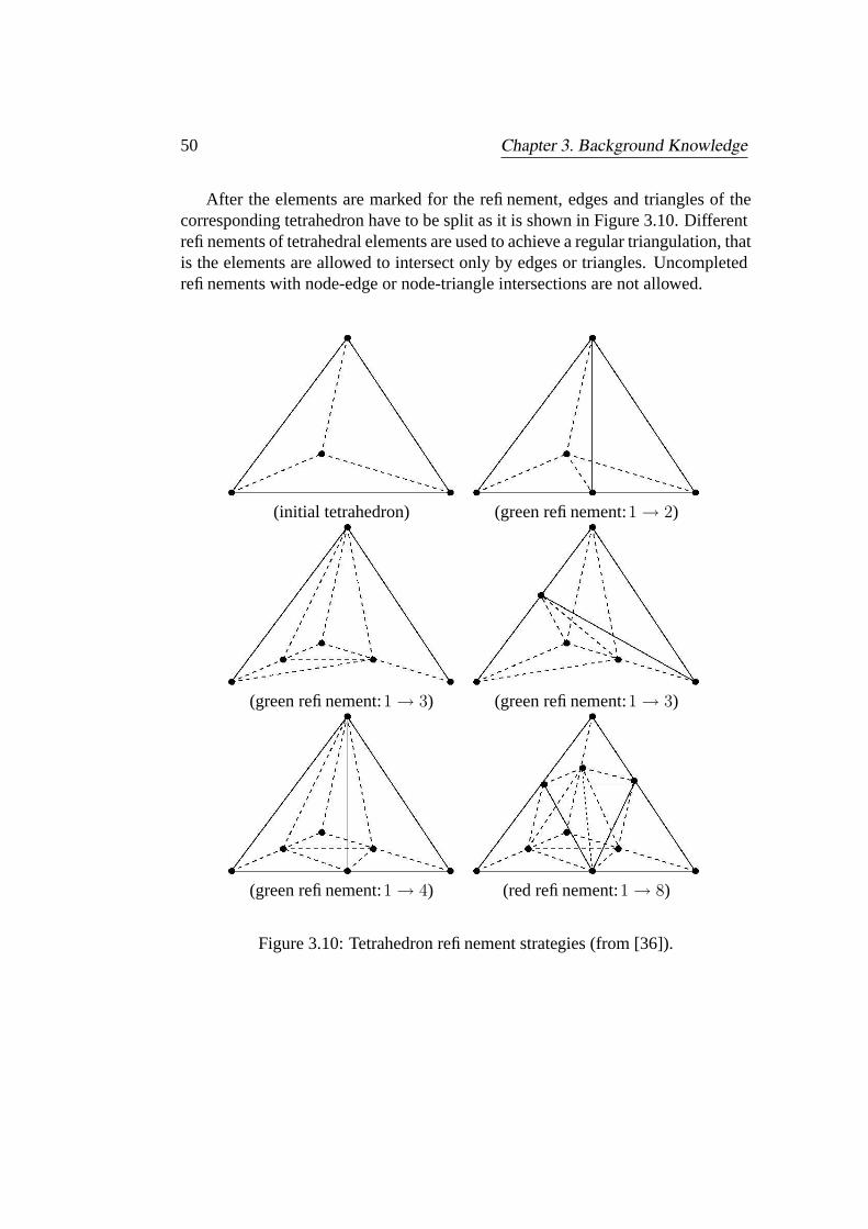
50 Chapter 3. Background Knowledge
After the elements are marked for the refinement, edges and triangles of thecorresponding tetrahedron have to be split as it is shown in Figure 3.10. Differentrefinements of tetrahedral elements are used to achieve a regular triangulation, thatis the elements are allowed to intersect only by edges or triangles. Uncompletedrefinements with node-edge or node-triangle intersections are not allowed.
(initial tetrahedron) (green refinement:1 → 2)
(green refinement:1 → 3) (green refinement:1 → 3)
(green refinement:1 → 4) (red refinement:1 → 8)
Figure 3.10: Tetrahedron refinement strategies (from [36]).

Chapter 4
Geometrical Modeling
The prerequisite for the adequate numerical simulation of soft tissue deformationsin the surgical planning is the correct reflection of individual anatomy in geomet-rical models. In this chapter, we describe the major steps needed to create a usefulvolumetric model of the patient’s anatomy from tomographic datasets. All artifi-cial objects as well as 3D human models presented in this work have been createdwith the help of the multipurpose visualization and modeling system Amira [112].
4.1 Image Segmentation
The 3D digital models of human anatomy are available as a set of 2D imagesgenerated with the help of computer tomography (CT) or magnetic resonanceimaging (MRI). The first step of the tomographic data processing is the importof medical image data. A typical CT slice is shown in Figure 4.1. The grey scalevalue of each pixel, the so-called Hounsfield unit (HU) of CT images is correlatedwith the intensity of X-ray scattering on different materials and differs from onetissue type to the other, which enables the identification of different anatomicalstructures and tissue regions, i.e. image segmentation. The task of medical im-age segmentation is the classification of different grey scale regions in accordancewith their anatomical meaning. Since different morphological structures do nothave a unique HU value, completely automatic segmentation of complex medicalimages is difficult and needs usually to be performed interactively with the helpof computer graphic tools, which enable semi-automatic detection and markingof different HU subregions. In Table 4.1, the approximate range of HU valuescorresponding to the different materials and tissue types is shown. The precisevalues depend on
51

52 Chapter 4. Geometrical Modeling
Figure 4.1: Typical CT slice.
Table 4.1: CT number range in HU.
Tissue HU values
Air -1000Lungs -1000 to -400Fat -100 to -50Water 0Brain 0 to 100Muscle 10 to 600Soft tissue -100 to 300Bone >500

4.2. Mesh Generation 53
• the operating conditions of the CT scanner in terms of kVp and filtration,
• the concrete patient,
• noise in the image with a standard deviation in the range ±3 to ±30 HU,
• any artifacts within the CT image, e.g., beam hardening,
and require an individual analysis and justification. Once the range of HU valuesfor different tissue types is defined, a preliminary automatic detection of substruc-tures and their boundaries can be applied, see Figure 4.2(top). Morphologicaloperators used for automatic segmentation are generally based on the recognitionof grey scale differences along the boundaries between the different HU regions[60, 107]. Images containing thin or small structures, artifacts or simply diffuseimages can be sometimes segmented only manually and require substantial timingexpenses.
In order to model and to simulate the biomechanic behavior of complex livingstructures, a range of properties and attributes varying from tissue to tissue andfrom element to element has to be taken into consideration. Most of these charac-teristics assigned already during the segmentation stage are further reflected in thehierarchically structured geometrical model. A final geometrical model basicallycontains lists of nodes, surface and volumetric elements, as well as the additionallists of id’s associated with these basic structures. Typically, the particular tissuetype (or material id associated with tetrahedra) and the conectivity between thedifferent tissue subregions (boundary id associated with triangles) are requiredfor modeling of the multi-composite tissue. Optionally, tetrahedron-, triangle- ornode-structures can be extended if further attributes are available such as the HUvalue on elements or nodes, for example.
4.2 Mesh Generation
With the digital tomographic data a natural discretization of continuous bodiesis given, see Figure 4.2 (bottom,left). However, the representation of 3D objectsas a set of 2D images consisting of pixels or corresponding 3D box-shaped ele-ments, voxels, requires substantial computational resources and is not optimal forthe visualization and the numerical simulation. On the one hand, natural volumet-ric voxel-based meshes can be easily parameterized and practically do not requireany additional expenses for mesh generation. On the other hand, such volumet-ric grids consisting of billions of nodes represent the huge amount of data, whichnowadays require the usage of massively parallel super-computers in order to per-form finite element calculations, and thus are not suited for interactive simulationsin an ordinary clinical environment.

54 Chapter 4. Geometrical Modeling
Figure 4.2: Top: image segmentation with Amira. Bottom: voxel-baseddiscretization (left), simplified surface model (middle), resulting tetrahedralmesh (right) (from [119]).

4.3. Mesh Quality Control 55
A state of the art approach for the geometrical modeling is the generation ofsurface models and is known as triangulation. Triangulated surfaces representthe boundaries between the different tissue regions. Surface models substantiallyreduce the original data amount and enable a compact representation of com-plex geometrical structures, see Figure 4.2 (bottom,middle). In this work, thecreation of surface models with correct topology and optimized triangular shapefrom the segmented tomographic data is carried out automatically with the helpof the marching cubes related algorithm provided with Amira [55]. Adaptive re-finement and coarsing of surface meshes is used to achieve an optimal resolutionof curved regions (for example in mouth, eye or nose areas) and at the same timeto keep the total number of elements as low as possible. For the numerical sim-ulation of continuum mechanics problems via the finite element method, a volu-metric mesh is needed. Meshes can be categorized as structured or unstructured[80]. Structured meshes exhibit uniform topological structure that unstructuredmeshes lack. In this work, an unstructured tetrahedral mesh generated on the ba-sis of the non-manifold surface triangulation is used, see Figure 4.2 (bottom,right).The generation of the tetrahedral meshes for an arbitrary 3D domain of interestis generally a difficult task. A useful mesh has to satisfy constraints that some-times seem almost contradictory. 3D mesh must conform to the object or domainbeing modeled, and ideally should meet constraints on both the size and shapeof its elements. The most popular approaches for tetrahedral mesh generationcan be divided into three groups: Delaunay triangulation [45, 111], advancingfront method [43], and methods based on grids, quadtrees or octrees. Tetrahedralmeshes used in this work are generated with the advancing front method. Thestarting point of advancing front algorithm is the triangulated surface. Trianglesof the discretized boundaries form the initial front. Tetrahedrons are generatedone-by-one, starting from the boundary edges or triangles and working towardthe center of the domain. The exposed inner faces of these elements collectivelyform an advancing front. Advancing front methods typically create good tetra-hedrons near the boundaries, but are less effective inside the domain, where thefronts collide. In Figure 4.3, stepwise advancing front triangulation of 2D domainis illustrated.
4.3 Mesh Quality Control
The accuracy of the finite element calculation depends on the quality of tetrahedralelement. One of the reasons is that the derivatives of the basis functions neededfor assembly of the elementary matrix are reciprocally proportional to the elementvolume ∇ϕ ∼ V −1
t . Degenerated tetrahedrons with small volume in conjuctionwith large displacements of the associated nodes may lead to large local errors

56 Chapter 4. Geometrical Modeling
Figure 4.3: Advancing front triangulation of 2D domain. Top row: initial bound-ary, 100 elements mesh. Bottom row: 500 elements mesh, final triangulation: 790elements mesh.
of the solution. In the worst case, the system of equations can even become un-solvable. This problem particularly concerns the linear basis functions, where thedisplacement gradient may become arbitrarily large, cf. (3.78). Even if all ele-ments are approximately of the same size, another criteria of the element qualitysuch as the maximal angle and the maximal edge length are important for theaccuracy of the FE solution. Theoretically, the FE solution should approach theexact solution of the given BVP as the size of the largest element approaches zero.However, in [2] it has been shown that if dihedral angles approach π as the elementsize decreases, convergence to the exact solution may fail. In Figure 4.4, typicaltetrahedral elements are shown, which have to be avoided in finite element calcu-lations for the above mentioned reasons. For the indication of the poor quality ofa tetrahedral element, different criteria are proposed. For the general characteri-zation of the element shape, the ratio between the circumsphere and the insphereR/r for the characterization of the element shape can be used, see Figure 4.5 (a).The tetrahedrons with the large quotient R/r should be avoided within the gridgeneration or eleminated ’a posteriori’. In particular, the elements with the largedihedral angle are critical for FE calculations, see Figure 4.5 (b). Additionally,criteria for element quality also depend on the nature of the concrete problem. Forphysical phenomena that exhibit anisotropic behavior, the most suitable elementshape may be the ”needle”. The effects of element shape on FE solutions are stillbeing investigated.

4.3. Mesh Quality Control 57
Figure 4.4: Bad tetrahedral elements (from [53]).
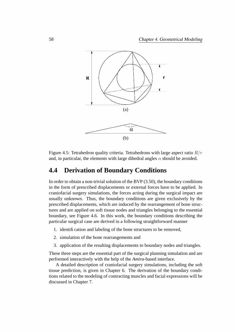
58 Chapter 4. Geometrical Modeling
(a)
(b)
Figure 4.5: Tetrahedron quality criteria. Tetrahedrons with large aspect ratio R/rand, in particular, the elements with large dihedral angles α should be avoided.
4.4 Derivation of Boundary Conditions
In order to obtain a non-trivial solution of the BVP (3.50), the boundary conditionsin the form of prescribed displacements or external forces have to be applied. Incraniofacial surgery simulations, the forces acting during the surgical impact areusually unknown. Thus, the boundary conditions are given exclusively by theprescribed displacements, which are induced by the rearrangement of bone struc-tures and are applied on soft tissue nodes and triangles belonging to the essentialboundary, see Figure 4.6. In this work, the boundary conditions describing theparticular surgical case are derived in a following straightforward manner
1. identification and labeling of the bone structures to be removed,
2. simulation of the bone rearrangements and
3. application of the resulting displacements to boundary nodes and triangles.
These three steps are the essential part of the surgical planning simulation and areperformed interactively with the help of the Amira-based interface.
A detailed description of craniofacial surgery simulations, including the softtissue prediction, is given in Chapter 6. The derivation of the boundary condi-tions related to the modeling of contracting muscles and facial expressions will bediscussed in Chapter 7.

4.4. Derivation of Boundary Conditions 59
Figure 4.6: Boundary value problem typically arising in the craniofacial surgicalplanning: find the deformation of a physical body occupying the domainΩ for theboundary conditions given by the prescribed displacements of its partial boundaryΓ′
e ⊂ Ω.

Chapter 5
Numerical Model
In this chapter, we discuss some applied aspects of the numerical model imple-mentation. First, we give a more precise statement of the problem from the com-putational point of view. Next, we investigate the sensitivity of the model withrespect to the variation of material parameters as well as their adequate scope forthe numerical simulation. Finally, the algorithmic implementation of the over-all adaptive numerical scheme of the non-linear elastic multilevel finite elementapproach is presented.
5.1 Simplified Numerical Model of Facial Tissue
In this section, we resume all previous discussions about the adequate simplifiedmodel of deformable facial tissue for the ”long term” prediction of patient’s post-operative appearance.
Simplified constitutive model. Complex material properties such as plastic andviscoelastic phenomena generally observed in soft tissue experiments may be ne-glected if the deformation is small or is performed over a period of time thatsuffices for recovery processes in living organism. For the ”long term” predictionof facial tissue, a simplified constitutive model based on a piecewise, isotropic,quasi-incompressible, non-linear hyperelastic material description is assumed.
Pure displacement problem. The original problem consists in the computationof the deformation for an object being under the impact of static loads implicitlygiven by the prescribed boundary displacements. Besides the displacement, nofurther physical terms describing the ”physics” of the surgical impact are avail-able. Thus, the most natural approach for the numerical modeling of such quasi-
60

5.2. Sensitivity Analysis and Parameter Estimation 61
geometric problem is to apply the so-called pure displacement FE discretizationof the BVP (3.50) as described in Section 3.3.
5.2 Sensitivity Analysis and Parameter Estimation
The existing literature on the mechanical properties of human tissues is abundant,but relatively scarce when one looks for converged, exact, comprehensive and rep-resentative data. There is a large scatter and uncertainty in the material propertiesof human tissue, according to sex, age, size, etc. Furthermore, there may be largedifferences found in tissue properties within an individual at different parts of thebody [54].
In our approach, each homogeneous and isotropic subdomain Ωi ⊂ Ω of acomposite elastic solid occupying the domain Ω is characterized by the stiffnessand the compressibility, which are described by two elastic constants, the Youngmodulus Ei and the Poisson ratio νi , respectively. Hence, we are concerned withthe estimation of the valid scope for (E, ν).
Quasi-incompressible material. The Poisson ratio is theoretically ranged inν ∈ [0, 0.5]. It is generally agreed that the adequate range for modeling of waterrich soft tissue is ν ∈ [0.4, 0.4(9)] [34, 44, 85, 90, 41]. However, the choice ofthe particular value for ν within this range has some far-reaching consequencesfor the type of the FE discretization approach. As we have mentioned above, thepure displacement FE discretization locks for ”almost incompressible” materialsν ≈ 0.5. The value of ν = 0.45 is considered as an admissible upper threshold forthe pure displacement FE method. Materials with ν > 0.45 have to be simulatedwith mixed finite elements, where the pressurep is treated as an independent vari-able in addition to the displacement u. Since the non-elliptic mixed formulationis much more computationally expensive in comparison with the efficient puredisplacement approach, the estimation of the quantitative difference between thequasi-incompressible ν = 0.45 and incompressible ν = 0.5 constitutive model isof a general interest.
Hence, we are going to estimate the modeling error in displacements corre-sponding to the Poisson ratio by studying the explicit dependence of some closeform solution of elasticity theory on ν. For this purpose, we use the so-called fun-damental solution of linear elasticity, see Appendix A. First, we write the normof the displacement (A.2) in the following form
u = A(f, r)B(ν, α) , (5.1)
where u = |u| and

62 Chapter 5. Numerical Model
Figure 5.1: Relative difference of the displacements for a compressible (ν < 0.5)and incompressible (ν = 0.5) medium as a function of the Poisson ratio RD|| =RD(ν, 0.5, α = 0), RD⊥ = RD(ν, 0.5, α = π
2) (see explanations in text).
A(f, r) =1
8π E
f
r,
B(ν, α) =1 + ν
1 − ν
√
(3 − 4ν)2 + cos2 α (7 − 8ν) .
(5.2)
We are interested in the estimation of the relative difference RD =∣
∣
∣
u(ν2)−u(ν1)u(ν1)
∣
∣
∣
RD =
∣
∣
∣
∣
AB(ν2) − AB(ν1)
AB(ν1)
∣
∣
∣
∣
=
∣
∣
∣
∣
B(ν2) −B(ν1)
B(ν1)
∣
∣
∣
∣
. (5.3)
(5.3) shows that the relative difference is a function of three variables RD =RD(ν1, ν2, α) and does not depend on f, r and E. Since RD weakly depends onthe angle to the vector of the acting force density RD(α) ∼ |cosα| , we observetwo extreme cases, namely RD|| = RD(α = 0) and RD⊥ = RD(α = π
2)
RD|| = RD(ν1 = 0.45, ν2 = 0.5, α = 0) = 0.034483,
RD⊥ = RD(ν1 = 0.45, ν2 = 0.5, α = π2) = 0.051724.
(5.4)
From (5.4), it follows that the relative difference of the displacements for a quasi-incompressible (ν = 0.45) and incompressible (ν = 0.5) material lie in the rangebetween 3.4% and 5.2% in every point of the domain Ω occupied by a body. InFigure 5.1, RD|| = RD(ν, 0.5, 0) and RD⊥ = RD(ν, 0.5, π
2) as functions of
ν ∈ [0, 0.5] are plotted.
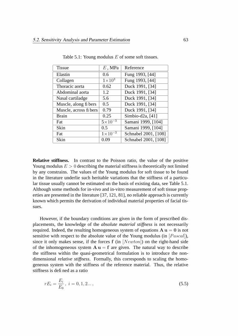
5.2. Sensitivity Analysis and Parameter Estimation 63
Table 5.1: Young modulus E of some soft tissues.
Tissue E , MPa Reference
Elastin 0.6 Fung 1993, [44]Collagen 1×10³ Fung 1993, [44]Thoracic aorta 0.62 Duck 1991, [34]Abdominal aorta 1.2 Duck 1991, [34]Nasal cartiladge 5.6 Duck 1991, [34]Muscle, along fibers 0.5 Duck 1991, [34]Muscle, across fibers 0.79 Duck 1991, [34]Brain 0.25 Simbio-d2a, [41]Fat 5×10⁻³ Samani 1999, [104]Skin 0.5 Samani 1999, [104]Fat 1×10⁻³ Schnabel 2001, [108]Skin 0.09 Schnabel 2001, [108]
Relative stiffness. In contrast to the Poisson ratio, the value of the positiveYoung modulusE > 0 describing the material stiffness is theoretically not limitedby any constrains. The values of the Young modulus for soft tissue to be foundin the literature underlie such heritable variations that the stiffness of a particu-lar tissue usually cannot be estimated on the basis of existing data, see Table 5.1.Although some methods for in-vivo and in-vitro measurement of soft tissue prop-erties are presented in the literature [37, 121, 81], no reliable approach is currentlyknown which permits the derivation of individual material properties of facial tis-sues.
However, if the boundary conditions are given in the form of prescribed dis-placements, the knowledge of the absolute material stiffness is not necessarilyrequired. Indeed, the resulting homogeneous system of equations Au = 0 is notsensitive with respect to the absolute value of the Young modulus (in [Pascal]),since it only makes sense, if the forces f (in [Newton]) on the right-hand sideof the inhomogeneous system Au = f are given. The natural way to describethe stiffness within the quasi-geometrical formulation is to introduce the non-dimensional relative stiffness. Formally, this corresponds to scaling the homo-geneous system with the stiffness of the reference material. Thus, the relativestiffness is defined as a ratio
rEi =Ei
E0
, i = 0, 1, 2... , (5.5)

64 Chapter 5. Numerical Model
Table 5.2: Absolute vs. relative stiffness.
material ID absolute stiffness, Ei relative stiffness, rEi
0 E0 11 E1 E1/E0
2 E2 E2/E0
3 E3 E3/E0
... ... ...n En En/E0
where Ei is the absolute stiffness of the i-th material and E0 is the absolute stiff-ness of the reference material. As long as no forces in [Newton] are given, theabsolute stiffness Ei can be replaced by rEi. The first trivial consequence of(5.5) is that in the case of only one material (homogeneous domain) the choiceof the Young modulus is practically irrelevant for the resulting deformation, sincerE0 = E0/E0 = 1. If the domain Ω consists ofN subdomains Ωi ⊂ Ω (piecewisehomogeneous domain) with Ei such that Ei 6= Ej , i 6= j, merelyN−1 unknownparameters rEi are needed to describe such multi-composite material, see Table5.2. If the domain of interest consists of only two tissue types, for example, mus-cle (M )and skin (S), merely one unknown parameter, namely, the ratio EM/ES
has to be estimated.
Stiffness estimation from CT scans. In computer assisted surgery, patient’sdata are represented with the tomographic images. Since the grey scale value,especially, in the case of CT images correlates with the physical properties ofscanned material, these data can be used for the estimation of the local tissuestiffness. The grey scale value (HU : Hounsfield unit) correlates to the densityHU ∼ ρ and in turn the Young modulus is a function of the density [16, 1]
E(ρ) = A+Bρp , (5.6)
where A, B and p are some real number constants. Thus, the implicit mappingHU → ρ → E should be generally possible. In [74], such mapping E(HU)in the form of a heuristic graph is proposed. However, there is no establishedderivation of the closed-form function E(HU) or more detailed investigation ofsome heuristic relationships between E and HU for soft tissue.
5.3. Details of Implementation 65
5.3 Details of Implementation
In this section, we give an overview of some aspects of the computational imple-mentation of our numerical model.
General software remarks. Finite element modeling and FE-based materialengineering, in particular, is one of the oldest, but still the most extensive domainsof computational physics and mathematics. The FEM incorporates a plethora ofnested complex mathematical and programming technical problems, which makesthe FEM software difficult to develop, to understand and to use. Indeed, modernFEM code has to provide
• flexible and efficient handling of arbitrary grids
• adaptive mesh refinement
• clear interface for physical problem definition, including
– PDE operator discretization in appropriate functional space
– constant parameter variation/control
– type of numerical integration
– type of problem solver
• efficient adaptive numerical techniques for assembling and solving the re-sulting system of equations based on error estimators
• user defined IO
• dynamic memory handling
The existing FEM packages do provide a useful user interface for FE analysis.However, most of them are extensive and expensive commercial software pack-ages still requiring a lot of time to learn by ropes.
At the very beginning of this work, first linear elastic FE analysis has beenperformed with the help of Kaskade toolkit [36]. We developed the FEM code,which was used in further investigations presented in the next chapters. In whatfollows, the basic concept of this software is described.
The C source code (400 kB) comprises more than 200 routines and functionsand is based on the following structures.

66 Chapter 5. Numerical Model
//—————————————————————————————-
struct double x[3]; // node coordinatesdouble u[3]; // node displacementdouble du[3]; // displacement incrementdouble f [3]; // nodal loadsdouble df [3]; // load incrementint nNbs; // number of node neighborsint ∗nb; // array of node neighbors nb[nNbs]double ∗A; // nodal stiffness A[3 ∗ 3 ∗ nNbs]int nNbTd; // number of neighbor tetrahedraint ∗ndTd; // array of neighbor tetrahedra ndTd[nNbTd]int nNbTr; // number of neighbor trianglesint ∗ndTr; // array of neighbor triangles ndTr[nNbTr]int nNbEd; // number of neighbor edgesint ∗ndEd; // array of neighbor edges ndEd[nNbEd]
meshNd; // mesh node
//—————————————————————————————-
struct int edNode[2]; // edge nodesint markerId; // multipurpose marker Id
meshEd; // mesh edge
//—————————————————————————————-
struct int trNode[3]; // triangle nodesdouble n[3]; // outer normalint bId; // boundary condition Idint sId; // surface type Id
meshTr; // mesh triangle
//—————————————————————————————-
struct int tdNode[4]; // tetrahedral nodesint markerId; // multipurpose marker Idint mId; // material type Id
meshTd; // mesh tetrahedron

5.3. Details of Implementation 67
//—————————————————————————————-
struct int nNds; // number of nodesmeshNd ∗nd; // array of nodes nd[nNodes]int nEds; // number of edgesmeshEd ∗ed; // array of edges ed[nEds]int nTrs; // number of trianglesmeshTr ∗tr; // array of triangles tr[nTrs]int nTds; // number of tetrahedrameshTd ∗td; // array of tetrahedra td[nTds]int nSrs; // number of surface patchesint ∗sr; // array of surface patches sr[nSrs]int nMts; // number of materialsint ∗mt; // array of materials mt[nMts]double ∗EMOD; // array of Young moduli EMOD[nMts]double ∗NU ; // array of Poisson ratios NU [nMts]
Mesh;
//—————————————————————————————-
This is only a brief overview of the very basic structures. At present, dozens ofattributes and parameters are required in our approach to describe composite facialtissue and to get a smart control on the FE computation of its deformation.
Adaptive algorithmic scheme. The overall algorithmic scheme for the adaptivecalculation of non-linear elastic deformations is shown in Figure 5.2.
From our findings, the adaptivity of the numerical scheme on different levelsof problem solving is essential for the achievement of the efficient and robustperformance. The main adaptive features of our approach include
• adaptive mesh refinement,
• adaptive linear/non-linear assembly of stiffness matrix,
• adaptive solving scheme, incl. PCG, ordinary and simplified Newton-PCG.
Hardware platforms. The numerical model for soft tissue simulations is de-veloped for the application in the clinical environment on comparatively low-costhardware platforms. The computations presented in this work are performed onan SGI Onyx II with 195MHz as well as on PC Pentium PIII with 600MHz and128MB RAM.

68 Chapter 5. Numerical Model
Figure 5.2: Overall algorithmic scheme.

Chapter 6
Static Soft Tissue Prediction
In this chapter, the results of experimental investigations carried out with artifi-cial objects as well as with the geometric models of real patients derived fromtomographic data are presented. Some general aspects of the FEM modeling ofdeformable objects can be gathered by studying simple artificial objects being un-der the impact of predefined loads. We focus on the comparison of the numericalresults with the theory, the effects of the mesh refinement as well as the com-parison between the linear and non-linear elastic approaches. Finally, we applyour approach for the prediction of the patient’s postoperative appearance in thesurgical planning of large and small bone rearrangements.
6.1 Experiments with Artificial Objects
The experiments with artificial objects are carried out (i) to compare the result ofthe finite element simulation with the theory, (ii) to quantify the difference be-tween the linear and non-linear elastic approach and (iii) to validate the advancedmodeling techniques with simple 3D objects.
Linear elastic model. In order to validate the numerical simulation of the ob-ject deformation, one ideally needs a closed-form solution of the given problem.Unfortunately, there are very few examples of closed-form solutions in three-dimensional structural mechanics. One of such closed-form solutions is the so-called fundamental solution of the Lame-Navier PDE, which describes the de-formation of an infinitely extended linear elastic medium under the impact ofthe Dirac-delta distributed force density, see Appendix A. The fundamental so-lution yields the deformation (the displacement field) for every point of infinitemechanical continuum as a function of coordinates u(x). An infinitely extendedmedium Ω∞ cannot be trivially discretized by finite elements. However, an arbi-
69

70 Chapter 6. Static Soft Tissue Prediction
Figure 6.1: Cubic subdomain of infinitely extended elastic continuum being underthe impact of the force density applied at the point O.
trary shaped subdomain Ω ⊂ Ω∞ can be understood as a separate elastic body withconstraints given on its boundary by the prescribed displacements of all surfacepoints ∀x , x ∈ Γ ⊂ Ω. Consider a cubic subdomain of Ω∞ as shown in Figure6.1. The force applied at the point O generate a displacement field in the wholedomain Ω∞. Since the fundamental solution for the Dirac-delta distributed forcedensity (A.2) is singular in the source O, we use the singularity-free solution de-rived for the Gauss distributed force density (A.5), which predicts theoretical dis-placements of both boundary and inner points of the test cube uT (x) ∀x , x ∈ Ω.Further, in accordance with the Somigliana’s identity [8]: the displacement of anarbitrary inner point P of a homogeneous linear elastic domain is uniquely de-scribed by the boundary displacements ui(Q) and tractions ti(Q)
ui(P ) =
∫
Γ
u∗i (P,Q)tj(Q)dS −∫
Γ
t∗i (P,Q)uj(Q)dS . (6.1)
Thus, we can formulate the following boundary value problem for the discretedomain ΩN :
Compute the displacements of inner nodes uN(x) ∀x , x ∈ Ω for the pre-scribed boundary displacements uN(x) ∀x , x ∈ Γ.
Consequently, the results of the FE simulation uN(x) for inner nodes of thecube ∀x , x ∈ Ω have to be compared with the theoretically predicted displace-ments uT (x) for these nodes.
This strategy is applied in conjunction with the verification of the domain re-finement. For this purpose, we consider four levels of uniform refinement of the

6.1. Experiments with Artificial Objects 71
(27 nodes) (125 nodes)
(729 nodes) (4913 nodes)
Figure 6.2: Uniform refinement of cubic domain.
Figure 6.3: Comparison between the FEM solution and the theory along the lineprobe AB (Figure 6.1) for different levels of domain discretization (Figure 6.2).

72 Chapter 6. Static Soft Tissue Prediction
cubic domain (see Figure 6.2):
0-level (initial discretization): 27 nodes (48 tetrahedra),
1-level: 125 nodes (384 tetrahedra),
2-level: 729 nodes (3072 tetrahedra),
3-level: 4913 nodes (24576 tetrahedra).
The comparison is carried out as follows:
1. First, the theoretical displacement uT for N points of the cube are calcu-lated by setting their coordinates in (A.5). The material properties are definedwith rE = 1 and ν = 0.4. The direction of the force F is set along the line probeAB, i.e. α = 0, cf. Figure 6.1.
2. Then, the displacements uN of inner nodes of the cube with the samematerial properties are computed via the linear elastic FEM for the boundary con-ditions given by the prescribed displacements of surface nodes as described above.
3. The relative difference |uT − uN |/|uN | for each node along the line probeAB (see Figure 6.1) is measured.
In Figure 6.3, the results of this comparison are shown. The effect of thedomain refinement is clearly seen in the reduction of the numerical error by factor2 as predicted by the theory. The maximum relative difference between the FEMand the theory in this example amounts up to 1.5%.
Linear vs non-linear elastic model. The comparison between the linear andnon-linear elastic approach is carried out with a simple artificial model consistingof a cylindric object with isotropic and homogeneous material properties, see Fig-ure 6.4 (a). The boundary conditions are given by the prescribed displacements atthe top of the cylinder, see Figure 6.4 (b). The associated boundary value prob-lem is solved both by applying the linear and non-linear elastic FEM, see Figure6.4 (c,d). It can be seen that the non-linear calculation yields significantly smallerdisplacements in comparison with the linear one, which is the direct result of thehigher ”geometrical stiffness” predicted by non-linear elasticity. In Figure 6.4 (e),line probes for the linear and non-linear solution measured along the main axisof the cylinder are depicted. The linearization error in this example reaches themaximum value on the boundary and amounts up to about 20 percent!

6.1. Experiments with Artificial Objects 73
(a) (b)
(c) (d)
(e)
Figure 6.4: (a): undeformed cylindric object, (b): boundary conditions on the topof the cylindric object, (c,d): comparison between the linear and non-linear elasticdeformation of a cylindric object, (e): line probes for the linear and non-lineardeformation measured along the main axis of the cylinder.

74 Chapter 6. Static Soft Tissue Prediction
Convergence behavior in dependence on ν. The Poisson ratio is the criticalparameter of the pure displacement FEM. When the Poisson ratio approaches 0.5,the condition number of the stiffness matrix rapidly increases and the convergenceof the PCG method becomes extremely bad. In Figure 6.5, the number of PCG it-erations required to achieve the predefined precision of the solution in dependenceon the Poisson ratio is shown. This diagram shows that convergence rate of thePCG method becomes extremely worse for ν > 0.45. Thus, we consider ν = 0.45as an admissible upper threshold for the approximation of a quasi-incompressiblematerial via the pure displacement FEM.
Figure 6.5: Convergence rate of the PCG method as a function of ν.
Sliding contact modeling. Besides the essential and natural boundary condi-tions (BC), special boundary constraints arise in the soft tissue modeling. Forinstance, contacts between lips and teeth, skin and muscles appear as a kind ofsliding. Sliding can be modeled as the homogeneous essential BC with respectto the local surface normal. To demonstrate the effect of sliding, following ex-periment is carried out. We consider a cylindric object under the impact of theforce density acting across the XY -plane from ”north-west” to ”south-east” , seeFigure 6.6 (top). The top of the cylinder is fixed. In Figure 6.6 (middle), the defor-mation of the cylinder with the natural BC on the remaining boundary is shown.Figure 6.6 (bottom) illustrates the deformation with the sliding contact constraintu(x)T n(x) = 0 at the cylinder bottom.

6.1. Experiments with Artificial Objects 75
Figure 6.6: Top: undeformed cylindric object. Middle: deformation without slid-ing contact constraint. Bottom: deformation with sliding contact constraint on thecylinder bottom.

76 Chapter 6. Static Soft Tissue Prediction
6.2 Soft Tissue Prediction in the CAS Planning
In this section, we present the experimental results of the soft tissue predictionwithin the craniofacial surgery planning. The experiments are carried out on thebasis of geometrical models derived from preoperative CT data. Since postop-erative tomographic data for the same patient are not available, we concentrateour efforts on the qualitative and indirect quantitative validation of the simulationoutcome. For the qualitative evaluation, the surgeons are consulted. In order toquantify the modeling error, e.g., the error produced by the linear elastic approx-imation or the particular material description, one even do not need the ”correctsolution”, since the modeling approach, as for instance the linear elastic FEM,implies the appropriate indicators for error detection itself.
Clinical case I. Large deformation. In the first example, the complete surgicalplanning of a juvenile patient with congenital mandibular hypoplasia, includingthe soft tissue prediction, is simulated, see Figure 6.7. The correcting surgi-cal impact for this patient consists in the calus (mandible) distraction, which isshown in Figure 6.8. The total maximum displacement of bone structures for thispatient amounts up to nearly 40mm, which cannot be classified as small deforma-tion anymore. Such extremely large bone rearrangement is performed by surgeonsstepwise over several months with the help of mechanical distractor device. Eachstep consists in an advancement of mandibula by approximately 1mm per day.Both the linear and non-linear elastic FEM are applied for the static prediction ofthe patient’s postoperative appearance [50, 51].
Linear elastic approach. First, the deformation of facial tissue is computed step-wise with the linear elastic approach. The results of the soft tissue prediction foreight steps, each one associated with the mandible distraction of 0.4− 0.6cm, areshown in Figure 6.9. Since the calus distraction has not yet been completed, adirect comparison with the postoperative data is not possible. Thus, we are inter-ested in the quantification of the error caused by the disregard of the geometricalnon-linearity in the linear elastic approach. In order to quantify the lineariza-tion error, a criterion based on the monitoring of the maximum component of thelinearized strain tensor ε = max|∇u | is used, cf. (3.22). The correction of non-linear elasticity, i.e. the contribution to the non-linear terms of the strain tensor,is of the order o(ε2). This means that ε indicates the relative linearization error.Further, the percentage of tetrahedrons with ε exceeding a certain threshold εi ismonitored. The results of the monitoring of the relative linearization error in de-pendence on the intensity of the deformation (cf. Figure 6.9 (a-h)) are shown inTable 6.1 as well as in Figure 6.10 (top). We give an example of how to in-terpret these data. Consider the entry in the third row (ε3 = 0.05) and the e-th
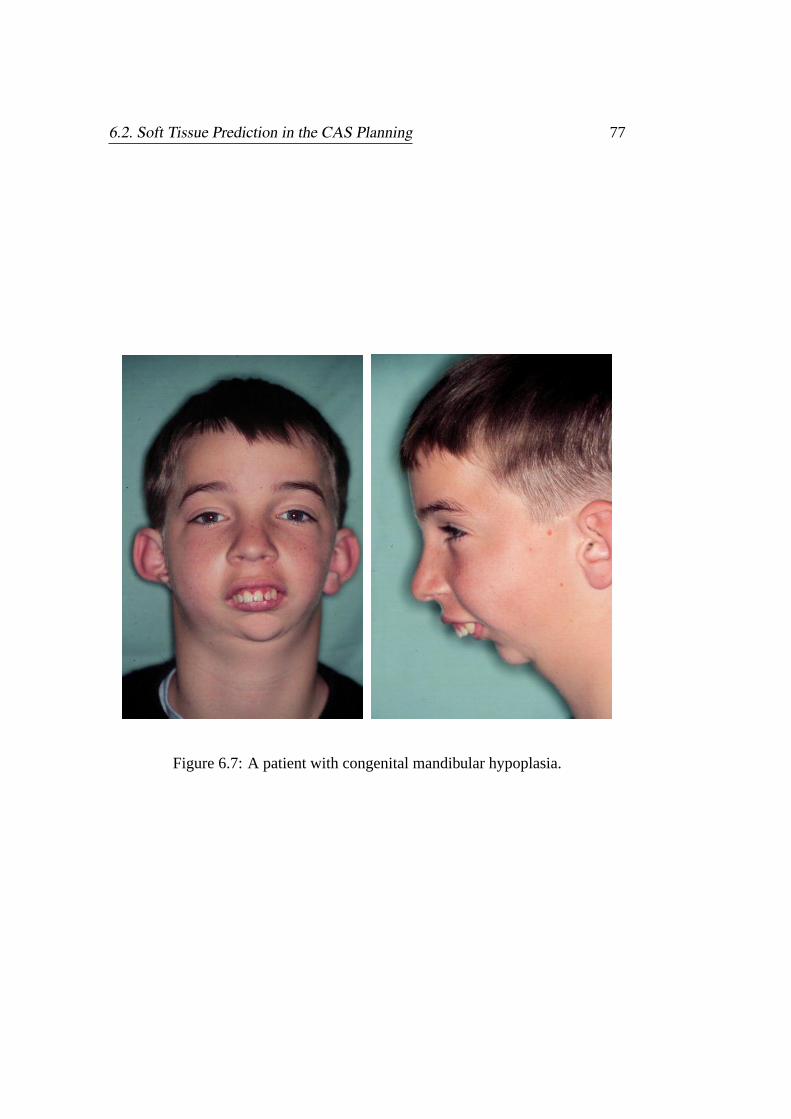
6.2. Soft Tissue Prediction in the CAS Planning 77
Figure 6.7: A patient with congenital mandibular hypoplasia.

78 Chapter 6. Static Soft Tissue Prediction
Figure 6.8: Simulation of mandible distraction.

6.2. Soft Tissue Prediction in the CAS Planning 79
(undeformed) (a) (b)
(c) (d) (e)
(f) (g) (h)
Figure 6.9: Resulting soft tissue deformation induced by the stepwise rearrange-ment of bone structures with maximal boundary displacements of: (a) 0.6cm, (b)1.2cm, (c) 1.6cm, (d) 2.0cm, (e) 2.6cm, (f) 2.8cm, (g) 3.3cm, (h) 3.8cm.

80 Chapter 6. Static Soft Tissue Prediction
Figure 6.10: Top: distribution of the linearization error in dependence on theintensity of deformation, cf. Figure 6.9 (a-h). Bottom: percentage of tetrahedronswith ε > 5% in dependence on maximum boundary displacements.

6.2. Soft Tissue Prediction in the CAS Planning 81
Figure 6.11: Top: 2D plain cut through a patient’s head, grey-scale gradient in-dicates the spatial distribution of deformation represented by the norm of the dis-placement vectors. Bottom: decrease of the displacement field measured alongthe line probe: from the ”source” B (bone) to S (skin).

82 Chapter 6. Static Soft Tissue Prediction
Table 6.1: Validation of the linearization condition ε 1 , cf. Figures 6.9 (a-h).
εi percentage [%] of tetrahedrons with ε > εia b c d e f g h
0.01 42.8 48.0 50.1 51.9 53.7 53.8 53.9 54.30.03 26.5 37.4 41.7 44.3 46.2 46.3 46.8 47.10.05 17.1 29.3 35.6 39.2 42.0 42.3 42.8 43.40.07 11.8 23.7 30.5 34.9 38.5 39.1 39.9 40.70.1 7.9 16.8 24.5 29.6 33.9 34.9 35.9 36.80.2 2.8 7.5 12.0 17.2 24.0 25.3 25.6 27.80.3 1.3 4.3 7.2 10.3 16.2 18.1 19.8 21.40.4 0.8 2.5 4.9 6.9 10.9 12.8 14.8 16.50.5 0.6 1.7 3.3 5.1 7.7 8.9 10.7 12.60.6 0.5 1.3 2.3 3.8 5.7 6.6 7.9 9.60.7 0.4 0.9 1.7 2.9 4.5 5.1 6.0 7.40.8 0.3 0.7 1.3 2.2 3.5 3.9 4.7 5.80.9 0.3 0.6 1.1 1.8 2.8 3.4 4.0 4.71.0 0.2 0.5 0.9 1.4 2.3 2.8 3.4 3.9
column (maximum boundary displacement of 2.6cm): 42.0%. This value meansthat in the case of the maximum boundary displacement of 2.6cm (cf. Figure6.9e) for 42.0% of all tetrahedrons the relative linearization error lie over 5%, i.e.ε > 0.05. In Figure 6.10 (bottom), the percentage of tetrahedrons with ε > 0.05in dependence on maximum displacement is depicted. The error curve shownin this diagram has no particular break-points, which would indicate the optimalstep width for the linear calculation. In contrast, the strongest increase of theerror-curve occurs on relative small displacements (duplication of error for maxi-mum boundary displacements in the range of [0.6, 1.6]cm), which trivially meansthat the smaller step width produces the smaller linearization error. Consequently,the optimal step width as well as the corresponding precision of the linear elasticcalculation are up to user. For the maximum deformation of 3.8cm (see Table6.1 (h)), the relative linearization error amounts more than 5% for nearly half ofall tetrahedra (43.4%). However, the analysis of spatial distribution of the lin-earization error shows that the largest error is concentrated inside of the patient’shead in the direct vicinity of relocated bone structures. In contrast, on the facialsurface, which is most important for an optical impression, one can hardly see anyartifacts. This fact can be explained through the r−1 decrease of the displacementfield with increasing distance from the source in3D, see Figure 6.11.

6.2. Soft Tissue Prediction in the CAS Planning 83
The computation of the deformation for a grid of 63.320 nodes (314.043 tetra-hedra) via the linear elastic FEM took 1.8 minute (residual norm of PCG algo-rithm: 10−10). The calculations are performed on an SGI Onyx II with 195MHzas well as on PC Pentium PIII with 600MHz.
Non-linear elastic approach. The linear elastic approximation of large defor-mations produces a substantial error caused by the disregard of the geometricalnon-linearity. Thus, the non-linear elastic approach is applied for the soft tissueprediction. For this purpose, the adaptive non-linear elastic FEM is used. Theresults of the soft tissue prediction computed with the non-linear elastic approachvs the linear elastic one are shown in Figure 6.12. The deformation computed viathe non-linear elastic approach is significantly smaller in comparison with the out-come of the linear elastic FEM, which yields too large deformations, particularlyin the chin area, see Figure 6.13.
By the computation of the non-linear elastic deformation some numericalproblems occur. After the first linear elastic step (cf. Figure 5.2) by higher or-der Newton iterations, the assembled system of equations sometimes becomesunsolvable due to the large condition number. The same problem concerning theiterative calculation of large deformations via the nonlinear elastic FEM has beenreported in [95] in application to elastic image registration. We have found thatthe reason for such fatal errors lies in the strong dependence of the non-linearelastic calculation on the displacement gradient ∇u, which cannot be computedaccurately if the initial grid contains degenerated elements and/or the inconsis-tent boundary conditions. In turn, the deeper reason for these failures lies in theviolation of the topology-preserving condition (3.6), which can be used for theindication of the failure occurrence.
This problem concerns only the non-linear elastic FEM, since the successivecomputation of the displacement gradient is not required for the linear elasticFEM. The handling of this problem is not easy and basically can be classified intotwo general groups of measures
(i) ’a priori’ measures: quality control of the initial mesh and consistencyproof of the applied boundary conditions,
(ii) ’a posteriori’ measures: monitoring of the displacement gradient w.r.t. thetopology-preserving condition.
In this work, ’a priori’ measures, i.e. extensive checking and improvement ofthe quality of the initial mesh and the applied boundary conditions, already help

84 Chapter 6. Static Soft Tissue Prediction
Figure 6.12: Simulation of large soft tissue deformation via the linear (top) andnon-linear (bottom) elastic approach.

6.2. Soft Tissue Prediction in the CAS Planning 85
Figure 6.13: Comparison between the facial outline predicted by the linear (outerline mesh) and non-linear (inner shaded mesh) elastic model.

86 Chapter 6. Static Soft Tissue Prediction
to fix the problem. However, the non-linear elastic approach appears generallymore sensitive with respect to the small abnormalities of input data and thus lessrobust as the linear elastic FEM.
The performance of the adaptive non-linear elastic FEM is quite satisfactory.The calculation of the non-linear solution on the same grid took approximately 7minutes, which corresponds to 4 iterations of the Newton method.
Clinical case II. Small deformation. In the next example, the postoperativeappearance of a patient with maxillary retrognatism and mandibular prognatismis simulated, see Figure 6.15 (top). Figure 6.14 illustrates the simulation of thecorrective surgical impact (bimaxillary osteotomy), which consists in an advance-ment of maxilla by 10mm and a set-back of mandibula by 12mm. The resultingsoft tissue deformation is simulated with the linear and non-linear elastic FEM. InFigure 6.15 shows pre- and postoperative picture of the patient. In Figure 6.16, thecomparison between the results of the linear and non-linear calculation is shown.Since the deformation in this case is relatively small, the linear solution matcheswell with the postoperative picture of the patient, see Figure 6.16 (1). However, aslight difference between postoperative and simulated profile outline in the nosearea can be seen, Figure 6.16 (2). The non-linear solution yields better result, Fig-ures 6.16 (3,4). Apparently, the reduction of this difference is due to the smallerdisplacement computed via the non-linear elastic FEM similar to the previouslyobserved examples, cf. Figure 6.4 and 6.13. The remaining difference can bereduced by a higher stiffness of the nasal cartilage, which has not been taken intoaccount by this simulation.
In this example, the linear elastic deformation for a grid of 106.166 nodes(504.112 tetrahedra) is computed in 2.9 minutes (residual norm of PCG algo-rithm: 10−10) on the same hardware platform (SGI Onyx II with 195MHz as wellas on PC Pentium PIII with 600MHz). The calculation of the non-linear elasticdeformation took 9.3 minutes, which corresponds to 3 iterations of the Newtonmethod.
Model sensitivity w.r.t. material parameters. Since soft tissue in our approachis modeled as a hyperelastic material, two elastic constants controlling the stiff-ness and the compressibility of each subdomain occupied by a different tissuelayer are required.
Facial tissue stiffness. In the examples of static soft tissue prediction, facial tis-sue is firstly approximated as a 1-component homogeneous material. The simula-

6.2. Soft Tissue Prediction in the CAS Planning 87
Figure 6.14: Simulation of bimaxillary osteotomy, including the soft tissue pre-diction.

88 Chapter 6. Static Soft Tissue Prediction
Figure 6.15: A patient with maxillary retrognatism and mandibular prognatism.Top: preoperative picture. Bottom: postoperative picture.

6.2. Soft Tissue Prediction in the CAS Planning 89
(1) (2)
(3) (4)
Figure 6.16: (1): validation of the linear elastic model, (2): nose area of (1), (3):validation of the non-linear elastic model, (4): nose area of (3).
90 Chapter 6. Static Soft Tissue Prediction
tion results in the absence of explicitly given forces are not sensitive with respectto the Young modulus E describing the material stiffness. The simulations carriedout with piecewise homogeneous approximation considering the different tissueregions have not shown any significant difference by the variation of the Youngmoduli of each particular tissue region in a ”reasonable range” of values of Ei.However, the multi-layer model with different tissue stiffnesses becomes impor-tant for the modeling of facial expressions, where the deformations are inducedby the impact of muscle forces, see Section 7.5.
Facial tissue compressibility. Quasi-incompressibility of soft tissue is modeledin this work with the Poisson ratio of up to ν = 0.45. In previous sections,we have already addressed the problems concerning the numerical modeling ofquasi-incompressible materials. Now, we validate the sensitivity of the modelingapproach with respect to the Poisson ratio by the direct comparison of the sim-ulation results for different ν ∈ [0, 0.45]. In Figure 6.17, the results of the softtissue prediction for ν = 0, 0.1, 0.2, 0.3, 0.4, 0.45 are shown. Being basicallypresent, the qualitative difference between the predicted facial surfaces can bevisually registered between a high and low compressible material behavior only,cf. Figures 6.17 (a-c) and (d-f), respectively. Taking into account that the de-formation simulated in this example is extremely large, the difference within therange of ν ∈ [0.3, 0.45] can be assumed neglectable and practically irrelevant forthe qualitative evaluation of the postoperative outcome. From our findings, thePoisson ratio of ν = 0.4 is a good compromise between the requirement of theconstitutive modeling and the computational performance.

6.2. Soft Tissue Prediction in the CAS Planning 91
(a) (b)
(c) (d)
(e) (f)
Figure 6.17: Results of soft tissue prediction for the Poisson ratio ν of (a): 0, (b):0.1, (c): 0.2, (d): 0.3, (e): 0.4, (f): 0.45.

Chapter 7
Individual Facial Expressions
Besides the static soft tissue prediction, the estimation of postoperative facialemotion expressions is another important criterion for the evaluation of the cran-iofacial surgery planning. The human face is an important and complex objectof human perception. Thus, the patients with facial deformities or paralysis areseverely limited in their abilities to the facial emotion expression and cannot con-vey the normal social signals of interpersonal communication. In such cases, thereestablishment of the aesthetical appearance and normal facial expressions is theprimary concern of the corrective surgical impact.
First, we summarize the particular goal of the estimation of facial emotionexpressions within the scope of the craniofacial surgery planning more precisely.Of course, the whole spectrum of individual facial emotion expressions is muchmore complex as it can ever be covered on the basis of abstract mechanical mod-els only. Because of a lack of information on the timing of individual muscularcontractions in our approach, the facial animation sequences, which we are ableto produce, will generally remain subjective. Nevertheless, consistent biomechan-ical modeling of facial expressions on the basis of individual anatomical modelsderived from tomographic data should yield some important insights about physi-cally possible individual facial emotion expressions. In fact, we are not pretendingto predict a typical smile of those individual, but one of his/her physically possibleexpression of happiness. This can be also formulated as follows: for example, thefacial expressions we are going to estimate are not necessarily the typical indi-vidual facial emotion expressions, but he/she should in turn be able to mime theway we figured. Besides the modeling of complex facial emotion expressions, theestimation of single muscle actions is of great interest for the non-surgical facialnerve rehabilitation [63].
The content of this chapter is as follows. After the review of the existing lit-
92

7.1. Facial Animation 93
erature related to the topic of facial animation and muscle modeling, we describeour approach for the modeling of contracting muscles and the estimation of in-dividual facial expressions. Finally, the experimental results of facial expressionsimulations are presented.
7.1 Facial Animation
The complexity of the human face makes it a challenging subject for modelers.It benefits from and can contribute to the larger field of human body modeling.Facial modeling is a multidisciplinary effort, which has links to many other fieldssuch as medicine and engineering. In the last three decades, many research groupshave made their substantial contributions to this complex and fascinating fieldof study. In view of particular goals, different techniques have been developed.Generally, the collective term of facial animation comprehends following threedisciplines [96]
• facial expression,
• facial conformation,
• lip motion (for speech synchronization).
The goal of the facial expression modeling is the modeling of the six canonical ex-pressions of happiness, anger, fear, surprise, disgust and sadness. Conformationcontrol specifies individual faces from the universe of possible face prototypesthat can be also associated with morphological or long-term facial changes, suchas growth or aging. Lip synchronization concerns the coordination of the jaw, lip,and mouth parts with real or synthetic speech samples. In this work, we focus onthe estimation of basic facial expressions only.
Four distinctive control techniques are known in the facial animation. These are
1. 3D shape interpolation,
2. ad hoc surface shape parameterization,
3. muscle-based, or abstract muscle models and
4. physically based models.
Each technique possesses particular advantages and disadvantages.

94 Chapter 7. Individual Facial Expressions
Shape interpolation is an early simple technique to control synthetic faces [91].It operates on a database of discrete facial postures, which are created from 3Ddigitizers or optical scanners. These facial datasets have the property of topolog-ical equivalence such that a complete mapping can be found for each vertex inevery facial posture. Once a complete set is derived, then in between interpolationof the coordinates can be computed. Unfortunately, this technique is limited tothe set of predefined facial postures, which prompted the development of param-eterization schemes.
The objective of facial parameterization is to describe the face with a small setof control parameters [92, 93]. These parameters are hard-wired into a particularfacial geometry and the parameters are only loosely based on the dynamics of thefacial expression. For example, the expression on the brow from surprise involvesthe manipulation of five or six vertices of the facial geometry. Alternatively, dis-tances measured between some facial landmarks (such as lip internal height orwidth) can be used to predict 3D parametric contour functions. This is partic-ularly useful in the case of the lips, which follow regular rules of deformation.Landmark-based techniques are very popular in computer graphics, since they areefficient and flexible, when animating some cartoon-based characters. An exam-ple of this approach is the motion-capturing technique [39], which is based onthe monitoring of the facial landmarks movements in the source image and theirmapping onto the target image. The main advantage of this approach is the adop-tion of the natural timing of human facial emotion expressions. Animated animalsand human characters in the recent computer animation based movies are realizedwith the help of this technique. Obviously, the motion capturing is not suited forthe estimation of individual facial expressions.
Muscle-based models or abstract-muscle models mimic at a simple level theaction of three primary muscle groups of the face: (1) the linear, such as the zy-gomaticus major, (2) the sphincter, such as the orbicularis oculi, and (3) the sheetsuch as the frontalis major [94, 82, 116]. This approach has also been extended toB-spline surfaces [115]. There are two distinct advantages for these models: theyare independent of particular facial geometry and they map directly into muscle-based coding systems.
Physically based models attempt to model the shape and dynamic changes ofthe face by modeling the underlying properties of facial tissue and muscle action[113, 100, 101]. Most of these models are based on mass-spring or FE mesheswith muscle actions approximated by a variety of force functions. These modelsare computationally expensive and difficult to control with force-based functions.As an example of this approach, in [71, 72] a framework for the estimation of

7.2. Anatomy and Physiology of Muscles 95
facial expressions based on a linear elastic FE model of soft tissue and a heuristicparametrization of the mimic muscles is presented.
Typically, the validity of facial animation sequences is done by visual inspec-tion. For example, does it look right? Such criterion might be sufficient for semi-realistic, cartoon-based faces. However, the goal of the facial expression simula-tion within the scope of craniofacial surgery planning is to estimate the individ-ual facial expressions. Simplified approaches, which do not consider individualanatomy and correct tissue biomechanics, are not adequate for that purpose. Fromthis point of view, there seems to be no alternative to consistent physical modelingof contracting muscles and muscle-tissue interaction on the basis of underlyingbiomechanical laws.
7.2 Anatomy and Physiology of Muscles
The main macroscopic property of muscle is its ability to contract. In accordancewith the sliding filament theory, this macroscopic property is effected through theshortening of muscle fibers that consist of two main contractile proteins (actin,myosin) and several other protein structures building a separate morphologicalunit, the so-called sarcomer [44]. Thereby, muscle fibers do get shorter due to asort of sliding of the myofilaments across each other. The shortening of the seri-ally arranged sarcomers develop a tension along their longitudinal axis. Sarcomersrepresent the lowest level of the complex hierarchical structure of muscles, whichis shown in Figure 7.1. The muscle fibers group themselves into bundles known asfascicles, which are in turn enveloped by a material known as fascia. Each fasciagroup represents different heads of a muscle. Within the fascia, the muscle fiberscan have an orientation characterized by the angle they make with respect to thetendons they attach to. This fiber arrangement is known as the muscle pennation.Figure 7.2 illustrates several types of pennation patterns of skeletal muscle. Thepennation patterns of facial muscles can be reduced to three main types alreadymentioned above: linear, sphincter and sheet.
The arrangements of muscle fibers determine the direction of the producedforces. Muscles can attach to tendon material either at a narrow site or over widesheets of tendon known as aponeurosis. As both muscle and tendon work closelytogether to create a functional unit of force generation and transmission, they areoften referred as a collective biomechanical structure, a musculotendon unit.
Tendon is made up of parallel-aligned collagen fibers (cf. Figure 3.1), whichare several orders of magnitude stiffer than muscle, cf. Table 5.1. Therefore, the

96 Chapter 7. Individual Facial Expressions
Figure 7.1: Hierarchical structure of muscles (from [44]).

7.2. Anatomy and Physiology of Muscles 97
Figure 7.2: Pennation patterns of skeletal muscles (from [85]).

98 Chapter 7. Individual Facial Expressions
areas where tendon is in contact with muscle have restricted movement comparedto the uncovered portions of muscle. The tendon portion of the skeletal muscu-lotendon unit attached to bone at two different sites known as the origin and theinsertion. Facial muscles differ from most other skeletal muscles in several sig-nificant ways. In particular, some mimic muscles are attached to soft tissue orother muscles. In this case, we call the tendon portion of the musculotendon unitattaches to bone the origin and those connected to soft tissue the insertion.
7.3 Biomechanical Models of Contracting Muscles
Any consistent geometrical and physical model of the musculotendon unit shouldcapture the aspects of muscle anatomy and physiology described above. Puttingit all together, muscles are represented in the geometrical model by their shapeand in the biomechanical model of deformable soft tissue by the forces actingalong the fiber tangents. Being vectorial variable, the force is characterized bythe magnitude and the direction. For an arbitrary shaped muscle occupying thedomain Ωmuscle, both the magnitude and the direction of the spatially distributedforce density f(x) are unknown functions of coordinates. For dynamical simula-tions of muscle contraction, time dependence of natural muscle activation patternsf(x, t) is additionally to be taken into account.
Hence, we firstly review existing abstract muscle models. The majority ofthese works has been done on the field of musculoskeletal biomechanics. How-ever, some general principles are still valid for any contracting muscles, includingthe facial musculature.
One of the earliest models of contracting muscle extensively used in laterworks is the so-called Hill’s model [58]. It is based on a series of controlledexperiments on muscle, namely the force-length and force-velocity dependenciesobserved in active muscle. The model has three major components: the serieselement (SE), the parallel element (PE) and the contractile element (CE). In thesimplified models, one of these elements can be removed, if they do not have asignificant effect on forces generated. The series element (SE) describes the ef-fects of several biological materials in musculotendon. This element representsmainly the elastic effects of tendon and intrinsic elasticity of structures within thesarcomer. The parallel element (PE) represents passive elastic properties of theconnective tissue sheaths (fascia) of the muscle. Due to the material properties ofthese sheaths, tension is only produced when the PE is actively strained beyondits rest length. The contractile element (CE) contains the source of active forcegeneration. The total muscle response in Hill’s models is described by the force-
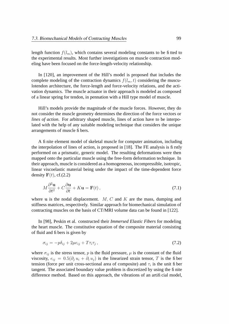
7.3. Biomechanical Models of Contracting Muscles 99
length function f(lm), which contains several modeling constants to be fitted tothe experimental results. Most further investigations on muscle contraction mod-eling have been focused on the force-length-velocity relationship.
In [120], an improvement of the Hill’s model is proposed that includes thecomplete modeling of the contraction dynamics f(lm, t) considering the muscu-lotendon architecture, the force-length and force-velocity relations, and the acti-vation dynamics. The muscle actuator in their approach is modeled as composedof a linear spring for tendon, in pennation with a Hill type model of muscle.
Hill’s models provide the magnitude of the muscle forces. However, they donot consider the muscle geometry determines the direction of the force vectors orlines of action. For arbitrary shaped muscle, lines of action have to be interpo-lated with the help of any suitable modeling technique that considers the uniquearrangements of muscle fibers.
A finite element model of skeletal muscle for computer animation, includingthe interpolation of lines of action, is proposed in [18]. The FE analysis is firstlyperformed on a prismatic, generic model. The resulting deformations were thenmapped onto the particular muscle using the free-form deformation technique. Intheir approach, muscle is considered as a homogeneous, incompressible, isotropic,linear viscoelastic material being under the impact of the time-dependent forcedensity F(t), cf.(2.2)
M∂2u
∂t2+ C
∂u
∂t+Ku = F(t) , (7.1)
where u is the nodal displacement. M, C and K are the mass, dumping andstiffness matrices, respectively. Similar approach for biomechanical simulation ofcontracting muscles on the basis of CT/MRI volume data can be found in [122].
In [98], Peskin et al. constructed their Immersed Elastic Fibers for modelingthe heart muscle. The constitutive equation of the composite material consistingof fluid and fibers is given by
σij = −pδij + 2µeij + Tτiτj , (7.2)
where σij is the stress tensor, p is the fluid pressure, µ is the constant of the fluidviscosity, eij = 0.5(∂j ui + ∂i uj) is the linearized strain tensor, T is the fibertension (force per unit cross-sectional area of composite) and τi is the unit fibertangent. The associated boundary value problem is discretized by using the finitedifference method. Based on this approach, the vibrations of an artificial model,

100 Chapter 7. Individual Facial Expressions
Figure 7.3: Fusiform, triangular and spiral muscle description (from [85]).
an immersed fiber-wound toroidal tube with two predefined layers of fibers is sim-ulated.
The major difficulty of themacroscopical modeling of muscles is the lack ofinformation on the unique, spatial arrangement of microstructures, e.g., musclefibers determining lines of acting forces. Especially in muscle-based facial ani-mation, an adequate interpolation of muscle forces is important for the realism ofthe resulting facial expression simulation. In previous works, a variety of heuristicconstructions considering the muscle anatomy has been proposed. Most of thesemodels use the mainline of muscle, i.e., the line connecting the origin and inser-tion areas, as line of action. Such mainline related model is used for the modelingof muscle-based facial expressions in [71, 72]. A model based on the fusiform in-terpolation of skeletal muscles is proposed in [106]. An interesting approach forthe interpolation of skeletal muscle forces based on B-spline technique is proposedin [89]. In [85], it has been intuitively remarked that muscle fibers are organizedresembling a flow, similar to the flow-lines considered in fluid mechanics or inelectromagnetism. Muscles may be viewed as continuous fibrous objects, whichmay be described by the means of a vector field acting along the fiber tangents.However, the author further considers only three predefined types of the penna-tion patterns: fusiform, triangular and spiral, see Figure 7.3. Any arbitrary shapedmuscle can then be represented by means of scaling of these three generic muscletypes.

7.4. Virtual Fibers 101
7.4 Virtual Fibers
Since none of the existing approaches known from the literature provides an ulti-mate solution for the biomechanical modeling of facial musculature, an alternativeapproach for modeling of individual muscle-based facial expressions is developedin this work.
In our approach, individual anatomy is represented in the geometrical modelby the triangulated surfaces, which correspond to the boundaries between essentialanatomical structures. However, the information on microscopic structures suchas fibers in muscles and skin needed for biomechanical modeling of anisotropicbehavior of these tissues is completely missing. In geometrical models, musclesare represented by the shapes of their infolding capsules. Since the information onmicroscopic structures such as muscle fibers cannot be obtained from tomographicdata, any suitable construction considering the natural relationship between mus-cle shape and its biomechanical functionality can be applied for the interpolationof spatial fiber arrangements.
Our approach for the estimation of individual facial expressions is based on theshape-based, heuristic construction of Virtual Fibers [52], which enables the inter-polation of muscle forces for an arbitrary shaped muscle embedded in the generalFE model of deformable facial tissue. In what follows, the essential statements ofthis approach are described.
Muscle forces. In the general FE model of deformable soft tissue, each muscleis represented by the 3 × N vector of nodal loads f , where N is the number ofmesh nodes, acting inside of the subdomain Ωmuscle ⊂ Ω along the direction offiber tangentsτ : |τ | = 1
f(x) =
λ(x) τ (x) x ∈ Ωmuscle ⊂ Ω
0 else(7.3)
where λ is the magnitude of the force density. Both λ(x) and τ (x) are generallyunknown functions of coordinates x.
Lines of action. The exact orientation of muscle fibers, i.e., the vector fieldof fiber tangents τ (x) in (7.3), which determines lines of acting forces, is un-known. The following construction is applied to interpolate τ (x) for the givenmuscle shape Γmuscle ⊂ Ωmuscle. Macroscopically seen, muscle fibers envelopedby the muscle capsule Γ3 connect two or more origin and insertion areas Γ1,2, seeFigure 7.4. The family of such geodesic curves reflecting the shape of the mus-

102 Chapter 7. Individual Facial Expressions
Figure 7.4: Schematic model of muscle: orientation of fibers connecting the originand insertion areas of muscle Γ1,2 reflects the muscle shape Γ3.
cle capsule seems in fact to yield a feasible interpolation of the natural fiber ar-rangement and resembles the iso-lines of a vector field observed in computationalthermodynamics, electromagnetismus, fluid or continuum mechanics. Accord-ingly, the spatial arrangement of muscle fibers can be obtained as a solution of theboundary value problem given by the partial differential equation of mathematicalphysics (PDEMF) and suitably defined boundary conditions. There is no particu-lar reason, which would make the interpolation technique based on one PDEMFmore accurate or advantageous in comparison with the others. However, we canimagine that at least one remark probably makes sense: the resulting vector fieldτ (x) should be preferably curl-free
[∇ × τ ] = 0 , (7.4)
which considers the fact that muscle fibers do not form knots. From (7.4), itfollows that τ is a gradient field
τ (x) = ∇ψ(x) , (7.5)
where ψ(x) is some scalar function of coordinates. Thus, the solution of theLaplace PDE
∇τ (x) = ∆ψ(x) = 0 x ∈ Ωmuscle ⊂ Ω (7.6)
with appropriate boundary conditions on Γmuscle ⊂ Ωmuscle will yield the curl-freevector field in the subdomainΩmuscle occupied by muscle.
However, in this work, we decided uniformly to use the PDEMF-solver al-ready available with our general FE platform based on continuum mechanics. Inthis approach, we obtain the interpolating field of fiber tangents as a kind oftestdeformation of the subdomain Ωmuscle corresponding to the muscle. Consider theschematic model of an unilateral muscle, cf. Figure 7.4. The test deformationyielding the vector field ofvirtual fiber tangents is given by the following linear
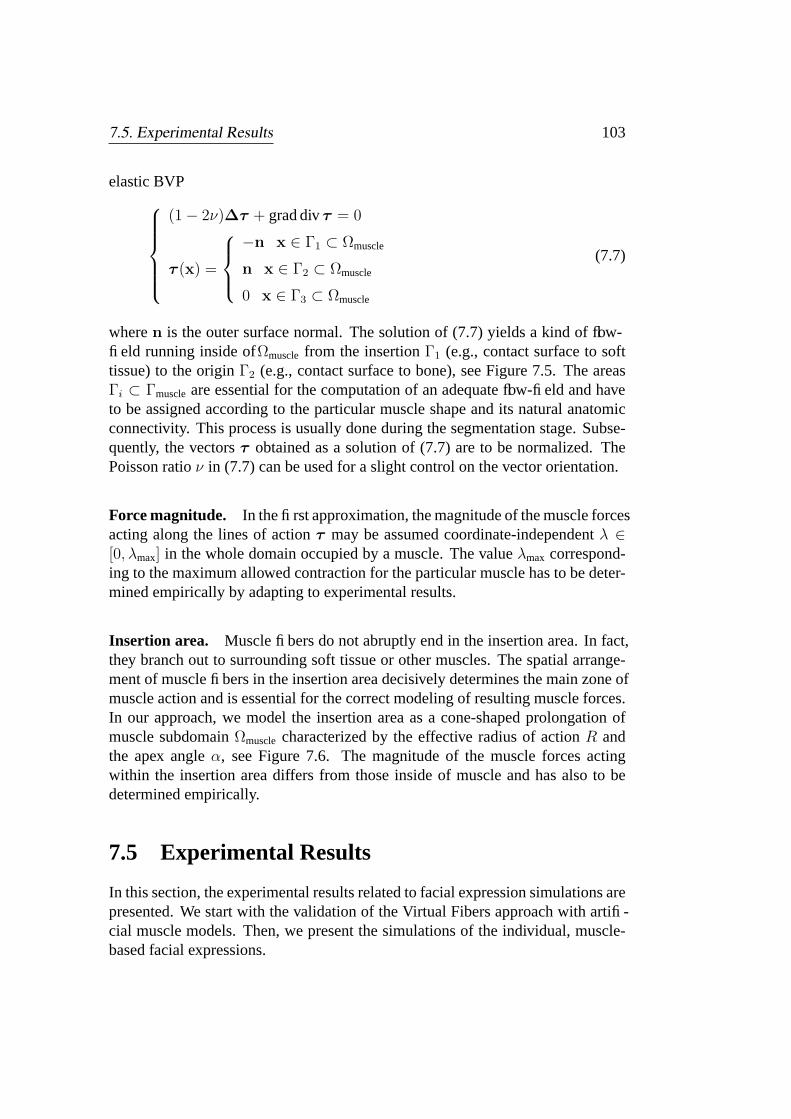
7.5. Experimental Results 103
elastic BVP
(1 − 2ν)∆τ + grad div τ = 0
τ (x) =
−n x ∈ Γ1 ⊂ Ωmuscle
n x ∈ Γ2 ⊂ Ωmuscle
0 x ∈ Γ3 ⊂ Ωmuscle
(7.7)
where n is the outer surface normal. The solution of (7.7) yields a kind of flow-field running inside ofΩmuscle from the insertion Γ1 (e.g., contact surface to softtissue) to the origin Γ2 (e.g., contact surface to bone), see Figure 7.5. The areasΓi ⊂ Γmuscle are essential for the computation of an adequate flow-field and haveto be assigned according to the particular muscle shape and its natural anatomicconnectivity. This process is usually done during the segmentation stage. Subse-quently, the vectors τ obtained as a solution of (7.7) are to be normalized. ThePoisson ratio ν in (7.7) can be used for a slight control on the vector orientation.
Force magnitude. In the first approximation, the magnitude of the muscle forcesacting along the lines of action τ may be assumed coordinate-independent λ ∈[0, λmax] in the whole domain occupied by a muscle. The value λmax correspond-ing to the maximum allowed contraction for the particular muscle has to be deter-mined empirically by adapting to experimental results.
Insertion area. Muscle fibers do not abruptly end in the insertion area. In fact,they branch out to surrounding soft tissue or other muscles. The spatial arrange-ment of muscle fibers in the insertion area decisively determines the main zone ofmuscle action and is essential for the correct modeling of resulting muscle forces.In our approach, we model the insertion area as a cone-shaped prolongation ofmuscle subdomain Ωmuscle characterized by the effective radius of action R andthe apex angle α, see Figure 7.6. The magnitude of the muscle forces actingwithin the insertion area differs from those inside of muscle and has also to bedetermined empirically.
7.5 Experimental Results
In this section, the experimental results related to facial expression simulations arepresented. We start with the validation of the Virtual Fibers approach with artifi-cial muscle models. Then, we present the simulations of the individual, muscle-based facial expressions.
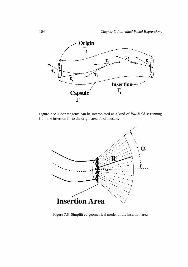
104 Chapter 7. Individual Facial Expressions
Figure 7.5: Fiber tangents can be interpolated as a kind of flow-field τ runningfrom the insertion Γ1 to the origin area Γ2 of muscle.
Figure 7.6: Simplified geometrical model of the insertion area.
7.5. Experimental Results 105
Artificial model. To validate the approach for modeling of contracting muscledescribed above, a simulation with a simple artificial model consisting of twonested cylinders is carried out, see Figure 7.7. In this artificial model, the innercylinder represents muscle and the outer cylinder corresponds to the remainingsoft tissue. The areas Γi in the BVP (7.7) required for the interpolation of fibertangents τ have been assigned as follows: Γ1 - the top, Γ2 - the bottom and Γ3 -the hull of the inner cylinder. The simulation shown in Figure 7.7 is performedwithin two following steps:
1. First, the vector field of fiber tangentsτ for the inner cylinder is calculatedby solving the BVP (7.7).
2. Then, the deformation of the surrounding material under the impact of theforce density f acting along the lines of action τ precalculated in step (1) is com-puted by solving the BVP (3.50) with the inhomogeneous right side. Thereby,the deformation of both cylinders in step (2) is computed with the homogeneousessential boundary conditions on the bottom of the outer cylinder Γessential, andnatural boundary conditions on the remaining boundary Γnatural.
Since the interpolated orientation of fibers in this example is trivial, namelyalong the main axis of the inner cylinder, the result of this simulation is as ex-pected.
Facial expressions: feasibility study. In the first feasibility study, the basicpostoperative facial expressions for the patient with congenital mandibular hy-poplasia (see Section 6.2) is estimated. The result of the static soft tissue predic-tion for this patient shown in Figure 6.12 was used as an input for further sim-ulation of muscle-based facial expressions. Figure 7.8 (a) shows the transparentgeometric model of the patient’s head with two mimic muscles, zygomaticus ma-jor left and right, which have been identified and segmented from CT data. Theseparticular mimic muscles raise the angle of mouth and are essential for normalsmile. Similar to the example with an artificial model, the surface of each muscleis subdivided into three areas Γ1,2,3 , cf. Figure 7.4: the area Γ1 corresponds to thecontact surface between muscle and bone (the origin), Γ2 is the contact surface tosoft tissue in the area of angle of the mouth (the insertion) and Γ3 is assigned tothe remaining muscle capsule. The simulation is performed as following:
1. First, the vector field of fiber tangentsτ for each muscle M is calculatedby solving the BVP (7.7) in ΩM with Γi ⊂ ΩM assigned as mentioned above.

106 Chapter 7. Individual Facial Expressions
Figure 7.7: From top to bottom, from left to right: allocation of areas Γi for theBVP (7.7), estimated orientation of virtual fibers, the original model, simulationof contraction of the inner cylinder and resulting deformation of the remainingmaterial.

7.5. Experimental Results 107
(a) (b)
(c) (d)
(e) (f)
Figure 7.8: Simulation of facial expressions induced by contraction of zygomati-cus major left and right. (a): 3D model of patient’s head, including muscles,(b): undeformed original surface model, (c-f): resulting soft tissue deformationinduced by the increasing contraction of two facial muscles.
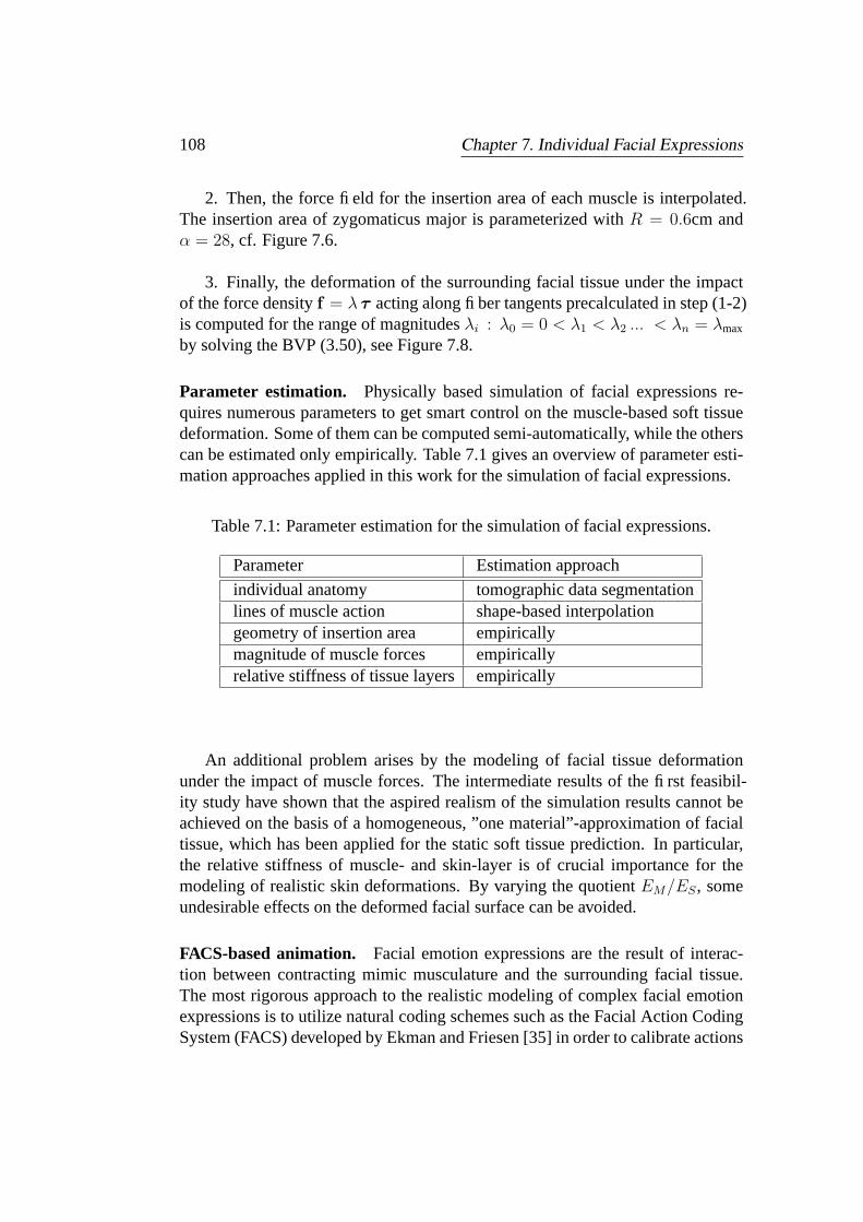
108 Chapter 7. Individual Facial Expressions
2. Then, the force field for the insertion area of each muscle is interpolated.The insertion area of zygomaticus major is parameterized with R = 0.6cm andα = 28, cf. Figure 7.6.
3. Finally, the deformation of the surrounding facial tissue under the impactof the force density f = λ τ acting along fiber tangents precalculated in step (1-2)is computed for the range of magnitudes λi : λ0 = 0 < λ1 < λ2 ... < λn = λmax
by solving the BVP (3.50), see Figure 7.8.
Parameter estimation. Physically based simulation of facial expressions re-quires numerous parameters to get smart control on the muscle-based soft tissuedeformation. Some of them can be computed semi-automatically, while the otherscan be estimated only empirically. Table 7.1 gives an overview of parameter esti-mation approaches applied in this work for the simulation of facial expressions.
Table 7.1: Parameter estimation for the simulation of facial expressions.
Parameter Estimation approach
individual anatomy tomographic data segmentationlines of muscle action shape-based interpolationgeometry of insertion area empiricallymagnitude of muscle forces empiricallyrelative stiffness of tissue layers empirically
An additional problem arises by the modeling of facial tissue deformationunder the impact of muscle forces. The intermediate results of the first feasibil-ity study have shown that the aspired realism of the simulation results cannot beachieved on the basis of a homogeneous, ”one material”-approximation of facialtissue, which has been applied for the static soft tissue prediction. In particular,the relative stiffness of muscle- and skin-layer is of crucial importance for themodeling of realistic skin deformations. By varying the quotient EM/ES , someundesirable effects on the deformed facial surface can be avoided.
FACS-based animation. Facial emotion expressions are the result of interac-tion between contracting mimic musculature and the surrounding facial tissue.The most rigorous approach to the realistic modeling of complex facial emotionexpressions is to utilize natural coding schemes such as the Facial Action CodingSystem (FACS) developed by Ekman and Friesen [35] in order to calibrate actions
7.5. Experimental Results 109
of different groups of facial muscles. The muscle-based abstraction provided byFACS maps well into a facial animation control strategy and has been used in anumber of facial animation systems [93, 72]. In Table 7.2, examples of FACS-coded facial emotion expressions are shown.
The coding of complex facial emotion expressions in accordance with FACSis formally equivalent to a superposition of single muscle actions yielding the totaldisplacement fieldu, i.e.,
u =∑
i
wiui (7.8)
where wi ∈ [0, 1] is the weighting factor of the displacement fieldui correspond-ing to i-th muscle action. However, (7.8) can strictly be used only for the linearelastic approximation of the soft tissue deformation. In the case of the non-linearapproximation, the deformation of soft tissue induced by the simultaneous con-traction ofN muscles cannot be reduced to the linear combination (7.8) and has tobe computed for every unique superposition of muscle actions anew by putting thetotal sum of all muscle forces
∑N
i f i into the right-hand side of the BVP (3.50).
Advanced simulations of facial expressions. The results of the first experi-mental study carried out with a relatively simple geometrical model have shownthat the simulation of complex facial emotion expressions on the basis of correctgeometrical models of human anatomy and consistent biomechanical approachesis feasible. To improve the realism of the simulation results, we further focus onthe following aspects:
1. Generalization of the modeling approach for the simulation of complex fa-cial emotion expressions requires more detailed geometrical models, including allgroups of mimic muscles.
2. Preliminary experimental results have shown that the parameters determin-ing the insertion area of linear muscles, i.e., its geometry and the acting forces,are decisive for the achievement of realistic results. Accordingly, the estimationof these parameters for each mimic muscle is important for the advanced simu-lations. Also, the modeling of sphincter muscles such as orbicularis oris requiresanother parameterization as in the case of linear muscles.
3. The realism of the first simulations was limited by the lack of subtle details,especially around the mouth. For instance, the contact between relatively thin lipsand teeth makes a non-trivial problem for the FEM-based modeling.

110 Chapter 7. Individual Facial Expressions
Table 7.2: FACS: Single Action Units (AU), cf. Figure 7.9.
AU No. FACS Name Muscular Basis
1 Inner Brow Raiser Frontalis, Pars Medialis
2 Outer Brow Raiser Frontalis, Pars Lateralis
4 Brow Lowerer Depressor Glabellae, Depressor Supercilli, Corrugator
5 Upper Lid Raiser Levator Palebrae Superioris
6 Cheek Raiser Orbicularis Oculi, Pars Orbitalis
7 Lid Tightener Orbicularis Oculi, Pars Palebralis
8 Lips Toward Orbicularis Oris
Each Other
9 Nose Wrinkler Levator Labii Superioris, Alaeque Nasi
10 Upper Lip Raiser Levator Labii Superioris, Caput Infraorbitalis
11 Nasolabial Furrow Zygomaticus Minor
Deepener
12 Lip Corner Puller Zygomaticus Major
13 Cheek puffer Caninus
14 Dimpler Buccinnator
15 Lip Corner Depressor Triangularis
16 Lower Lip Depressor Depressor Labii
17 Chin Raiser Mentalis
18 Lip Puckerer Incisivii Labii Superioris and Inferioris
20 Lip Stretcher Risorius
22 Lip Funneler Orbicularis Oris
23 Lip Tightner Orbicularis Oris
24 Lip Pressor Orbicularis Oris
25 Lips Part Depressor Labii or Relaxation of Mentalis or
Orbicularis Oris
26 Jaw Drop Masetter, Temporal and Internal Pterygoid
27 Mouth Stretch Ptergoids, Digastric
28 Lip suck Orbicularis Oris
38 Nostril Dilator Nasalis, Pars Alaris
39 Nostril Compressor Nasalis, Pars Transversa, Depressor Septi Nasi
41 Lid Droop Relaxation of Levator Palpebrae Superioris
42 Slit Orbicularis Oculi
43 Eyes Closed Relaxation of Levator Palpebrae Superioris
44 Squint Orbicularis Oculi, Pars Palpebralis
45 Blink Relaxation of Levator Palpebrae and
Contraction of Orbicularis oculi, Pars Palpebralis
46 Wink Orbicularis Oculi

7.5. Experimental Results 111
Figure 7.9: Top: mimic musculature, anterior view; middle: superficial muscles ofhead and mimic muscles, lateral view. Bottom: deep mimic musculature, lateralview (from [25]).

112 Chapter 7. Individual Facial Expressions
Detailed geometrical model of facial musculature. For the advanced simula-tion of facial emotion expressions, a detailed model of human head, including allgroups of mimic muscles, is generated. For this purpose, MRI volunteer data wereused, see Figure 7.11.
Parameterization of linear muscles. The parameterization of linear musclesbasically consists in the interpolation of fiber tangents for a given muscle shapeand the estimation of the insertion area parameters. Since the impact of a muscleon soft tissue is mainly concentrated in the insertion area, i.e., the magnitude ofthe effective forces acting within the insertion area is much larger than that of theforces inside the muscle, the vector field of fiber tangents (inside of muscle!)τ isnot critical for the modeling of single muscle actions and can be intrepolated withany suitable heuristic approach. Instead of the relatively circumstantial, physicallymotivated interpolation technique used in the first experimental study, we now ap-ply a B-spline based approach to estimate initial lines of muscle forces [118]. Thegeometrical parameters of the insertion area are estimated empirically. Table 7.3gives an overview of the insertion area parameters for some linear mimic muscles.
Table 7.3: Parameterization of the insertion area of some linear mimic muscles bythe effective radius R of action and the apex angle α, cf. Figure 7.6.
Muscle R, cm α
zygomaticus major 0.8 30zygomaticus minor 0.5 30risorius 0.5 25depressor angularis oris 0.7 28levator angularis oris 0.7 30depressor labii 0.4 30levator labii 0.4 30
Parameterization of sphincter muscles. Forces produced by the contractionof sphincter muscles are, in general, difficult to model on the basis of underly-ing ”sliding fibers” mechanism. For example, the impact of orbicularis oris on softtissue, i.e., the resulting mouth articulation, also depends on the reaction from theteeth. Continuum-based modeling of these phenomena is non-trivial. Instead ofthis approach, we apply a parameterization technique well known from computeranimation, which consists in a heuristic interpolation of sphincter muscles as anellipsoid contracting along its radial directions, see Figure 7.10.
7.5. Experimental Results 113
Figure 7.10: Simplified model of sphincter muscle.
Mouth area modeling. The contraction of most mimic muscles results in thedeformation of the mouth area. The movements of the lips as well as the resultingform of the mouth are essential elements of the facial emotion expressions. Thus,any incorrectness in the modeling of the mouth area immediately results in unre-alistic constraints between the lips and the teeth. In order to enable the natural lipsmovements, we now treat the contact between lips and teeth as ”unfixed”, i.e., thenatural (Neumann-like) or sliding boundary condition.
Simulation results. Since any facial emotion expression can be obtained as acombination of single muscle actions and basic mouth articulations (e.g., mandibleleft, right, up, down, forwards and backwards movements), we firstly compute allelementary sequences needed for the modeling of more complex facial emotionexpressions. Figure 7.12 illustrates the results of the simulation the basic articu-lation. The boundary conditions for these simulations are given by the prescribeddisplacements of mandible. In Figures 7.13-7.16, the simulation results of singlemuscle actions are shown. In the case of facial muscles, boundary conditions aregiven by the forces, which have been precalculated as described above. Based onthe entire set of precalculated single muscle actions, the complex facial emotionexpressions are simulated. Figure 7.17 demonstrates the simulation of a facialexpression of happiness estimated by superpositioning single muscle actions ofzygomaticus major, zygomaticus minor, risorius and orbicularis oris. Figure 7.18illustrates a facial expression of disgust simulated as a superposition of singlemuscle actions of depressor angularis oris left, depressor labii left, mentalis left,levator labii right and orbicularis oris left and right.

114 Chapter 7. Individual Facial Expressions
Figure 7.11: Detailed geometrical model of human head generated on the basisof MRI volunteer data (from [118]). Top: inner view, surface model of mimicmusculature. Bottom: outer view, skin surface.

7.5. Experimental Results 115
(a) (b)
(c) (d)
(e) (f)
Figure 7.12: Simulation of mandible articulation. (a): original model, lateral view.(b): original model, front view. Mandible movements: (c): forward, (d): right, (e):down, (f): left.

116 Chapter 7. Individual Facial Expressions
Figure 7.13: Simulation of single muscle action: zygomaticus major left.
Figure 7.14: Simulation of single muscle action: depressor angularis oris right.

7.5. Experimental Results 117
Figure 7.15: Simulation of single muscle action: levator labii right.
Figure 7.16: Simulation of single muscle action: mentalis left.

118 Chapter 7. Individual Facial Expressions
Figure 7.17: Simulation of facial expression of happiness by superpositioningsingle muscle actions of zygomaticus major, zygomaticus minor, risorius and or-bicularis oris.

7.5. Experimental Results 119
Figure 7.18: Simulation of facial expression of disgust by superpositioning singlemuscle actions of depressor angularis oris left, depressor labii left, mentalis left,levator labii right and orbicularis oris left and right.

Conclusion
We have carried out theoretical and experimental investigations leading to the de-velopment of the numerical model of facial tissue biomechanics for the predictionof the patient’s static postoperative appearance and facial emotion expressions incraniofacial surgery planning.
Since soft tissue generally shows a very complex biomechanical behavior, anadequate simplified model tailored to the particular range of problems is formu-lated. In craniofacial surgery planning, the essential input for the numerical mod-eling is usually given in the quasi-static and quasi-geometrical form, i.e., no in-formation on the timing of bone rearrangement, the acting forces or any otherphysical terms describing the ”physics” of the surgical impact is available. Thepostoperative patient’s appearance has to be predicted on the basis of 3D geomet-rical models derived from tomographic data and the prescribed displacements ofrelocated bone structures. For the estimation of facial expressions, the geometricmodel of patient’s anatomy is the only input for the further modeling.
Our approach for the general modeling of deformable facial tissue is basedon the non-linear elastic approximation of tissue biomechanics. Different tissuetypes are modeled as a homogeneous, isotropic, quasi-incompressible St. Venant-Kirchhoff material characterized by two elastic constants, the Young modulus Edescribing the material stiffness and the Poisson ratio ν describing the materialcompressibility. In our approach, we substitute the absolute material stiffness bythe non-dimensional relative stiffness rE, which can be easier estimated and re-duces the number of unknowns. Low compressibility of soft tissue is modeled bya Poisson ratio in the range ν ∈ [0.4, 0.45].
The numerical solution of the associated boundary value problem on tetrahe-dral grids is obtained via the finite element method (FEM). The linear elastic FEMwidely used in previous works is generally limited by the assumption of small de-formations and produces a substantial error by ad hoc calculations of large defor-mations, which are usual in the craniofacial surgery. Since the non-linear elastic
121

122 Chapter 7. Individual Facial Expressions
FEM is computationally very expensive, an adaptive numerical scheme is devel-oped. In order to achieve the efficient and robust performance, the adaptivity ofthe numerical scheme on different levels of problem solving is required. In ourapproach, we have implemented (i) the adaptive mesh refinement, (ii) the adap-tive linear/non-linear assembly of the stiffness matrix and (iii) the adaptive solvingscheme, whereby (i-ii) are based on efficient numerical indicators for the monitor-ing of the local deformation. For the solution of the resulting linear or non-linearelastic problem, the preconditioned conjugate gradient method (PCG) with Jacobipreconditioner, the Newton method and the simplified Newton method have beenimplemented.
The developed FE model has been validated in the experiments with the arti-ficial objects as well as by the direct comparison with the patient’s postoperativefacial outline. The outcome of the surgical impact on soft tissue induced by smalland large rearrangements of bone structures has been simulated. The resulting softtissue prediction has also been positively evaluated by collaborating surgeons.
In addition to the static soft tissue prediction, the modeling approach for theestimation of individual facial emotion expressions has been developed. We as-sume consistent biomechanical mechanism of facial expressions that is the impactof contracting muscles on remaining facial tissue. Numerous unknown parame-ters such as direction and magnitude of muscle forces, geometry of insertion areaof muscles as well as the material constants for a multi-layer model have to beestimated for the realistic simulation of facial tissue mechanics. The first stepin our modeling approach is the simulation of single muscle contraction. Sincethe information about microscopic structures, e.g., muscle fibers, cannot be ob-tained from tomographic data, any suitable construction considering the correctmuscle anatomy and biomechanics may be applied for the interpolation of mus-cle forces resulting from fiber tensions. The shape-based, heuristic technique ofvirtual fibers developed in this work enables the interpolation of muscle forcesfor an arbitrarily shaped muscle. In the general model of deformable soft tissue,muscles are represented by the force density acting along the fiber tangents. Usingthis technique, elementary facial emotion expressions resulting from single mus-cle actions have been simulated. On the basis of this ’database of single muscleactions’, complex facial emotion expressions are modeled.

7.5. Experimental Results 123
The investigations carried out in the present thesis have their origin in the clin-ical application and do provide the methodological basis for further application-oriented developments.
Outlook
The biomechanical modeling of living objects is a very challenging problem,which requires a comprehensive knowledge of different fields of study, e.g., biol-ogy, continuum mechanics, numerical mathematics. Especially, the advances inexperimental biomechanics providing more detailed constitutive models of livingtissues are the essential prerequisite for the development of more sophisticatedmodeling approaches. Quantitative, comprehensive and differentiated descrip-tion of static and time-dependent constitutive properties of different tissues is stillmissing.
Since this work is primarily devoted to the modeling, a numerical platformfor the FE simulation, which is relatively easy to implement and to control, isused. For the dimension of problems studied within the present work, i.e., gridsof ≤ 107 elements, this technique enable an acceptable performance. For signifi-cantly larger grids, the application of more sophisticated numerical methods, e.g.,multi-grid techniques, should be taken into consideration.
A general problem that remains the potential object of future research is the ac-curate and efficient computation of large deformations. The appropriate handlingof numerical problems associated with the calculation of the smooth orientation-preserving displacement gradient on large deformed FE grids should improve therobustness of the non-linear elastic FE calculation, which is essential for clinicalapplications.
Finally, the whole set of problems related to the increasing realism of facialexpression simulations still remains an interesting object of further investigations.Due to the encouraging results of experimental studies carried out in this work, wesee a high potential for more detailed simulations of muscle-based facial expres-sions on the basis of highly resolved geometrical models of human anatomy andmore sophisticated biomechanical approaches. The modeling of numerous subtledetails of human face, such as individual material properties depending on age,sex, nationality etc., wrinkles as well as various contact and obstacle phenomena,offers practically unlimited possibilities for perfectioning of simulation results.There is still a lot of work to do.

Appendix A
Notation
∅ empty set
R set of real numbers
Mn set of all real square matrices of order n
Ω bounded open subset of Rn
Γ boundary of Ω
L2(Ω) space of square integrablefunctions on Ω
Hm(Ω) Sobolev spaces of order m = 1, 2, . . .
‖ · ‖ norm in vector space
‖ · ‖2 Euclidean vector norm
‖ · ‖0,Ω norm in the space L2(Ω)
‖ · ‖m, Ω norm in a Sobolev space
albl =∑
i aibi Einstein’s sum notation
∂i = ∂/∂xi partial derivative with respect to xi
125

126 Chapter A. Notation
L differential operator
∆ Laplace-operator
∇ Nabla-operator
∇ · u = div u = ∂iui divergence of a vector field
∇φ = gradφ = (∂1φ1, . . . , ∂nφn)T gradient of a scalar function
∇u = ∂jui Jacobian of a vector field
I identity matrix
det(A) determinant of a matrix
tr(A) =∑
i aii trace of a matrix
‖x‖A =√
xTAx energy norm
λmin,max(A) min/max eigenvalue of a matrix
κ(A) = λmaxλmin
condition number of a matrix
e1, e2, . . . , en basis vectors in Rn
divT =∑
i
∑
j ∂jTijei divergence of a tensor field
a · b = aTb vector inner product
〈A,B〉 = tr(ATB) matrix inner product
u displacements
t tractions
n normal
σ second Piola-Kirchhoff stress tensor
ε strain tensor

127
λ, µ Lame constants
E Young modulus
ν Poisson ratio
C tensor of elastic constants
A(u) operator of non-linear elasticity
A′(u) Frechet derivative of A(u)

Appendix B
Fundamental Solution ofLinear Elasticity
A theoretical solution of the Lame-Navier PDE (3.54) can usually be found for avery limited number of boundary value problems with the special intrinsic sym-metry [38]. One of such important cases is the so-called fundamental solutionthat describes the deformation of an infinitely extended linear elastic medium un-der the impact of the Dirac-delta δ(x) distributed force density applied at the pointO (see Figure A.1)
E
2(1 + ν)(∆u +
1
1 − 2νgrad div u) = −fδ(x) , (A.1)
where f is a constant vector (not a function of coordinates). The fundamentalsolution of (3.54), also known as the Green’s function of linear elasticity is givenby
u =1 + ν
8πE(1 − ν)
(3 − 4ν)f + f cosα er
r, (A.2)
where f = |f | , r = |r| = |OP | is the vector from the starting point O to thespace point P , er = r/r is the unit vector in the direction of r and α is the anglebetween f and er , see Figure A.1. In elasticity theory, it can be shown that everysolution of an arbitrary linear elastic boundary value problem can be representedas a linear combination of fundamental solutions. The singularity of the funda-mental solution in the point O is the direct result of the ”unnatural” behavior ofthe Dirac-delta distribution
limr→0
u = ∞ . (A.3)
128

129
Figure A.1: Deformation of an infinite linear elastic medium under the impact ofthe Dirac-delta δ(x) distributed force density applied at the point O.
In [48], a singularity free solution of the Lame-Navier PDE for the Gauss-distributedforce density is derived
E
2(1 + ν)(∆u +
1
1 − 2νgrad div u) = − f
(√
2πσ)3exp(− r2
2σ2) , (A.4)
where σ denotes the characteristic width of the Gauss distribution. The solutionof (A.4) is given by
u =1 + ν
8πE(1 − ν)Φf (ξ)f + Φr(ξ)f cosα er , (A.5)
where
Φf (ξ) =
√2
σ (3 − 4ν) (ξ)
2 ξ+
(ξ)
4 ξ3− exp(−ξ2)
2√π ξ2
Φr(ξ) =
√2
σ (ξ)
2 ξ− 3 (ξ)
4 ξ3+
3 exp(−ξ2)
2√π ξ2
(A.6)
with ξ = r√2σ
. It can be easily shown that (A.5) converges to (A.2) for r σ andin the limit r → 0 remains regular
limr→0
u =(5 − 6ν)(1 + ν)
3(√
2π)3(1 − ν)Eσf . (A.7)

Bibliography
[1] M. Aisling et al. Anisotropic elastic properties of cancellous bone from ahuman edentulous mandible. In Proc. of ASME Bioengineering’99 Confer-ence, 1999.
[2] I. Babuska and A. K. Aziz. On the angle condition in the finite elementmethod. SIAM Journal on Numerical Analysis, 13:214–226, 1976.
[3] R. Bajcsy and C. Broit. Matching of deformed images. In Proc. 6-th Int.Conf. on Pattern Recognition, pages 351–353, Munchen, 1982.
[4] R. Bajcsy and S. Kovacic. Multiresolution elastic matching. ComputerVision, Graphics, and Image Processing, 46:1–21, 1989.
[5] A. H. Barr. Global and local deformations of solid primitives. In Proc. ofSIGGRAPH’84, 1984.
[6] R. Bartels, J. Beatty, and B. Barsky. An Introduction to Splines for usein Computer Graphics and Geometric Modeling. Morgan Kaufmann, LosAltos, 1987.
[7] P. I. Begun and J. A. Shukeilo. Biomechanics (in russian). Polytechnika.ISBN 5732503095, St.Petersburg, 2000.
[8] D. E. Beskos. Boundary Element Methods in Mechanics. North-Holland,Amsterdam, 1987.
[9] F. L. Bookstein. Principal warps: Thin-plate splines and the decomposi-tion of deformations. IEEE Transactions on Pattern Analysis and MachineIntelligence, 11(6):567–585, 1989.
[10] F. A. Bornemann, B. Erdmann, and R. Kornhuber. Adaptive multilevel-methods in three space dimensions. Int. J. for Numer. Meth. in Eng.,36:3187–3203, 1993.
131

132 Chapter A. Notation
[11] D. Braess. Finite Elemente: Theorie, schnelle Loser und Anwendungen inder Elastizitatstheorie. Springer, Berlin, 1997.
[12] C. A. Brebia. Boundary Element Techniques. Springer, Berlin, 1984.
[13] M. Bro-Nielsen. Fast finite elements for surgery simulation. In Proc. ofMedicine Meets Virtual Reality 5 (MMVR-5’97), 1997.
[14] M. Bro-Nielsen and S. Cotin. Real-time volumetric deformable modelsfor surgery simulation using finite elements and condensation. In Proc. ofEurographics’96 Conference, volume 15, pages 57–66, 1996.
[15] C. Broit. Optimal Registration of Deformed Images. PhD thesis, Universityof Pennsylvania, 1981.
[16] D. Cebon and M. F. Ashby. Materials selection for precision instruments.Meas. Sci. and Technol., 5:296–306, 1994.
[17] Y. Chang and A. P. Rockwood. A generalized de casteljau approach to 3Dfree-form deformation. In Proc. of SIGGRAPH’94 Conference, 1994.
[18] D. T. Chen and D. Zeltzer. Pump it up: Computer animation of a biome-chanically based model of muscle using the finite element method. Com-puter Graphics, 26:89–98, 1992.
[19] G. E. Christensen. Deformable Shape Models for Anatomy. PhD thesis,Washington University, August 1994.
[20] P. G. Ciarlet. The Finite Element Method for Elliptic Problems, volume 4 ofStudies in Mathematics and its Applications. North-Holland, Amsterdam,1978.
[21] P. G. Ciarlet. Mathematical Elasticity. Volume I: Three-Dimensional Elas-ticity, volume 20 of Studies in Mathematics and its Applications. North-Holland, Amsterdam, 1988.
[22] S. Coquillart. Extended free-form deformation: A sculpturing tool for 3Dgeometric modeling. In Proc. of SIGGRAPH’90 Conference, 1990.
[23] S. Cotin, H. Delingette, and N. Ayache. Real time volumetric deformablemodels for surgery simulation. In Proc. of VBC’96 Conference, 1996.
[24] M. A. Crisfield. Non-linear Finite Element Analysis of Solids and Struc-tures. John Wiley & Sons, Chichester, 1991.

133
[25] DAVID. Online atlas of human anatomy for clinical imaging diagnosis.URL: http://www.cid.ch/DAVID/Mainmenu.html.
[26] M. H. Davis. Deformable Matching of 3D Medical Images. PhD thesis,Southern Methodist University, May 1996.
[27] H. Delingette. Towards realistic soft tissue modeling in medical simulation.rapport de recherche no 3506. Technical report, INRIA, Le Chesnay Cedex,1998.
[28] X. Deng. A Finite Element Analysis of Surgery of Human Facial Tissues.PhD thesis, Columbia University, 1988.
[29] P. Deuflhard. A modified Newton method for the solution of ill-conditionedsystems of nonlinear equa tions with application to multiple shooting. Nu-mer. Math., 22:289–315, 1974.
[30] P. Deuflhard and A. Hohmann. Numerische Mathematik I. Walter deGruyter, Berlin, 2002.
[31] P. Deuflhard, P. Leinen, and H. Yserentant. Concepts of an adaptive hierar-chical finite element code. Impact of Computing in Science and Engineer-ing, 1:3–35, 1989.
[32] P. Deuflhard and M. Weiser. Local inexact Newton multilevel FEM fornonlinear elliptic problems. In M.-O. Bristeau, G. Etgen, W. Fitzigibbon,J. Lions, J.-L. a nd Periaux, and M. Wheeler, editors, Computational sci-ence for the 21st century, pages 129–138. Wiley, 1997.
[33] P. Deuflhard and M. Weiser. Global inexact Newton multilevel FEM fornonlinear elliptic problems. In W. Hackbusch and G. Wittum, editors,Multigrid Methods V, Lecture Notes in Computational Science and Engi-neering, pages 71–89. Springer, 1998.
[34] F. Duck. Physical properties of tissues: a comprehensive reference book.Academic Press, London, 1991.
[35] P. Ekman and W. Friesen. Unmasking the Face. A Guide to RecognizingEmotions From Facial Clues. Prentice-Hall, Englewood Cliffs, New Jersey,1975.
[36] B. Erdmann, J. Lang, and R. Roitzsch. KASKADE manual version 2.0:FEM for 2 and 3 space dimensions. Technical report, Zuse InstituteBerlin (ZIB), Berlin, 1993.
134 Chapter A. Notation
[37] R. Q. Erkamp, P. Wiggins, A. R. Skovoroda, S. Emelianov, andM. O’Donnell. Measuring the elastic modulus of small tissue samples.Ultrasonic Imaging, 20:17–28, 1998.
[38] H. Eschenauer and W. Schnell. Elastizitatstheorie. B.I. Wissenschaftsver-lag, Mannheim, 1993.
[39] Famous3D. Facial animation solutions. URL:http://www.famous3D.com.
[40] M. Ferrant, S. K. Warfield, C. R. G. Guttmann, R. V. Mulkern, F. A. Jolesz,and Kikinis R. 3D image matching using a finite element based elasticdeformation model. In Proc. of MICCAI’99 Conference, 1999.
[41] SimBio: A Generic Enviromet for Bio-numerical Simulation. Materialdatabase design report. URL: http://www.simbio.de.
[42] O. Forster. Analysis 3. Integralrechnung im IRn mit Anwendungen. Vieweg,Braunschweig, 1984.
[43] P. Frey and H. Borouchaki. Delaunay tetrahedralization using anadvancing-front approach. In Proc. of 5th International MeshingRoundtable, SAND’96, 1996.
[44] Y. C. Fung. Biomechanics - Mechanical Properties of Living Tissues.Springer, Berlin, 1993.
[45] P. L. George and H. Borouchaki. Delaunay Triangulation and Meshing.Hermes, Paris, 1998.
[46] P. Germain. Mecanique des Milleux Continus (russian edition). MIR,Moscow, 1965.
[47] S. F. F. Gibson and B. Mirtich. A survey of defomable modeling in com-puter graphics. TR-97-19. Technical report, Mitsubishi Electric ResearchLaboratory, Cambridge, 1997.
[48] E. Gladilin. Theoretische und experimentelle Untersuchung der lineare-lastischen Randelementemethode zur elastischen Registrierung medizinis-cher Bilder. Master’s thesis, Universitat Hamburg, Juli 1999.
[49] E. Gladilin, W. Peckar, K. Rohr, and H. S. Stiehl. A comparsion betweenBEM and FEM for elastic registration of medical images. TR FBI-HH-M-287/99. Technical report, FB Informatik, Hamburg University, Hamburg,1999.

135
[50] E. Gladilin, S. Zachow, P. Deuflhard, and H.-C. Hege. Validation of a linearelastic model for soft tissue prediction in craniofacial surgery. In Proc. ofSPIE Medical Imaging Conference, volume 4319, pages 27–35, San Diego,USA, 2001.
[51] E. Gladilin, S. Zachow, P. Deuflhard, and H. C. Hege. Adaptive nonlinearelastic FEM for realistic prediction of soft tissue in craniofacial surgerysimulations. In Proc. of SPIE Medical Imaging Conference, San Diego,USA, 2002.
[52] E. Gladilin, S. Zachow, P. Deuflhard, and H. C. Hege. Shape-based ap-proach for the estimation of individual facial mimics in craniofacial surgeryplanning. In Proc. of SPIE Medical Imaging Conference, San Diego, USA,2002.
[53] D. Guoy. Sink-insertion for mesh improvement. URL:http://www.cse.uiuc.edu/∼guoy/sink/.
[54] E. Haug. Biomechanical models in vehicle accident simulation. In Proc. ofPAM’95 Conference, 1995.
[55] H. C. Hege, M. Seebaß, D. Stalling, and M. Zockler. Generalized marchingcubes algorithm based on non-binary classifications. ZIB preprint SC-97-05. Technical report, Zuse-Institute-Berlin (ZIB), Berlin, 1997.
[56] D. Helm. Untersuchung der EAS-formulierung fr nahezu inkompressiblegummiartige materialien bei finiten deformationen. Master’s thesis, Uni-versitat Kassel, 1994.
[57] M. Hestenes and E. Stiefel. Methods of conjugate gradients for solvinglinear systems. J. Res. NBS, 49:409–436, 1952.
[58] A. V. Hill. The force-velocity relation in shortening muscle. first and lastexperiments in muscle mechanics. Cambridge at the University Press, 3,1970.
[59] N. Ng Hing and R. Grimsdale. Computer graphics techniques for modelingcloth. IEEE Computer Graphics and Applications, 16:28–41, 1996.
[60] K. H. Hohne and R. Berstein. Shading 3D-images from CT using gray levelgradients. IEEE Trans. on Medical Imaging, 5:45–47, 1986.
[61] G. A. Holzapfel. Nonlinear Solid Mechanics. John Wiley & Sons, Chich-ester, 2000.

136 Chapter A. Notation
[62] The human head. A resource for 3D modelers. URL:http://www.erc.msstate.edu/∼camen/thehumanhead/.
[63] Diels H. J. New concepts in nonsurgical facial nerve rehabilitation. Ad-vances in Otolaryngology-Head and Neck Surgery, 9:289–315, 1995.
[64] D. L. James. Multiresolution Green’s Function Methods for InteractiveSimulation of Large-scale Elastostatic Objects and other Physical Systemsin Equilibrium. PhD thesis, UBC, 2001.
[65] D. L. James and D. K. Pai. ARTDEFO: Accurate real time deformableobjects. In Proc. of SIGGRAPH’99 Conference, 1999.
[66] P. Kalra, A. Mangili, N. Magnenat Thalmann, and D. Thalmann. Simula-tion of facial muscle actions based on rational free form deformations. InProc. of Eurographics’92 Conference, 1992.
[67] M. Kass, A. Witkin, and D. Terzopoulos. Snakes: Active contour models.Int. Journal of Computer Vision, 1:321–331, 1988.
[68] M. Kauer. Inverse Finite Element Characterization of Soft Tissues withAspiration Experiments, Diss. No. 14233. PhD thesis, ETHZ, 2001.
[69] E. Keeve, S. Girod, and B. Girod. Craniofacial surgery simulation. In Proc.of VBC’96 Conferece, pages 541–546, 1996.
[70] R. M. Kenedi, T. Gibson, J. H. Evans, and J. C. Barbenel. Tissue mechanics.Phys. Med. Biol., 20:699–717, 1975.
[71] R. M. Koch, M. H. Gross, and A. A. Bosshard. Ein FEM-basierter Mimik-generator fur animierte anthropomorphe Avatare. In Proc. of AAA’97 Con-ference, volume 3, pages 31–40, 1997.
[72] R. M. Koch, M. H. Gross, and A. A. Bosshard. Emotion editing usingfinite elements. InProc. of Eurographics’98 Conference, volume 17, pages295–302, 1998.
[73] R. M. Koch, M. H. Gross, F. R. Carls, D. F. von Bren, and Y. I. H. Parish.Simulating facial surgery using finite element models. In Proc. of SIG-GRAPH’96 Conference, pages 421–428, 1996.
[74] R. M. Koch, S. H. M. Roth, M. H. Gross, A. P. Zimmermann, and H. F.Sailer. A framework for facial surgery simulation. technical report no. 326.Technical report, Computer Science Department, ETHZ, Zurich, 1999.

137
[75] R. H. Krause. Monotone Multigrid Methods for Signorini’s Problem withFriction. PhD thesis, FU Berlin, 2001.
[76] R. D. Kriz. Microstructure lestures. Technical report. Department of En-gineering Science and Mechanics, Virginia Polytechnic Institute and StateUniversity, 2000.
[77] L. D. Landau and E. M. Lifschitz. Elastizitatstheorie. Akademie-Verlag,Berlin, 1989.
[78] P. S. Laplace. Philosophical Essay on Probabilities. Springer, Berlin, 1995.
[79] Y. Lee, D. Terzopoulos, and K. Waters. Realistic modeling for facial ani-mation. In Proc. of SIGGRAPH’95 Conference, 1995.
[80] V. D. Liseikin. Grid Generation Methods. Springer, Berlin, 1999.
[81] H. Maass. Untersuchung einer Methode zur nichtinvasiven Messung vonSteifigkeitskoeffizienten an lebendem Gewebe mit multimodalen bildgeben-den Verfahren. PhD thesis, Universitat Karlsruhe, Marz 1999.
[82] N. Magnenat-Thalmann, N. E. Primeau, and D. Thalmann. Abstract muscleactions procedures for human face animation. Visual Computer, 3:290–297, 1988.
[83] G. E. Mase. Theory and Problems of Continuum Mechanics. McGraw Hill,New York, 1970.
[84] Y. Masutani et al. A new modal representation of liver deformation fornon-rigid registration in image-guided surgery. In Proc. of CARS’01 Con-ference, pages 19–24, 2001.
[85] W. Maurel, Y. Wu, N. Magnenat Thalmann, and D. Thalmann. Biomechan-ical Models for Soft Tissue Simualtion. Springer, Berlin, 1998.
[86] T. McInerny and D. Terzopoulos. Deformable models in medical imageanalysis: a survey. Medical Image Analysis, 1:91–108, 1996.
[87] D. N. Metaxas. Physics-based deformable models. Kluwer Academic Pub-lishers, Boston, 1997.
[88] C. Monserrat, V. Hernndez, M. Alcaiz, MC. Juan, and V. Grau. Evaluationand study of a new deformable model based on boundary element methods.In Proc. of CARS’99 Conference, 1999.

138 Chapter A. Notation
[89] V. Ng-Thow-Hing. Anatomically-based models for physical and geomet-ric recontruction of humans and other animals. PhD thesis, University ofToronto, 2001.
[90] N. Ozkaya and Nordin M. Fundamentals of Biomechanics. Springer,Berlin, 1999.
[91] F. I. Parke. Computer generated animation of faces. Master’s thesis, Uni-versity of Utah, UTEC-CSc-72-120, 1972.
[92] F. I. Parke. A model for human faces that allows speech synchronizedanimation. Computers and Graphics, 1:1–4, 1975.
[93] F. I. Parke and K. Waters. Computer Facial Animation. A K Peters, Welles-ley, 1996.
[94] M. Patel. Making FACES. PhD thesis, University of Bath, 1991.
[95] W. Peckar, C. Schnorr, K. Rohr, and H.S. Stiehl. Parameter-free elasticdeformation approach for 2-D and 3-D registration using prescribed dis-placements. Journal of Mathematical Imaging and Vision, 10(2):143–162,1999.
[96] K. Pelachaud, N. I. Badler, and M. L. Viaud. Final report ofthe standards for facial animation workshop, october 1994. URL:http://www.cis.upenn.edu.
[97] A. Pentland et al. Closed-form solutions for physically based shape model-ing and recognition. IEEE Transactions on Pattern Analysis and MachineIntelligence, PAMI-13(7):715–729, 1991.
[98] C. Peskin and D. McQueen. A three-dimensional computational method forblood flow in the heart.immersed elastic fibers in a viscous incompressiblefluid. Journal of Computational Physics, 81:372–405, 1989.
[99] G. Picinbono, H. Delingette, and N. Ayache. Real-time large displacementelasticity for surgery simulation: Non-linear tensor-mass model. In Proc.of MICCAI’00 Conference, pages 643–652, Pittsburgh, 2000.
[100] S. D. Pieper. CAPS: Computer-Aided Plastic Surgery. PhD thesis, M.I.T,Cambridge, 1991.
[101] S. Platt and N. Badler. Animating facial expressions. Computer Graphics,15:245–252, 1981.
139
[102] K. Rohr et al. Point-based elastic registration of medical image data usingapproximating thin-plate splines. In Proc. of VBC’96 Conference, volume1131 of Lecture Notes in Computer Science, pages 297–306, Hamburg,September 1996. Springer.
[103] S. H. M. Roth, M. H. Gross, S. Turello, and F. R. Carls. A bernstein-bzier based approach to soft tissue simulation. In Proc. of Eurographics’98Conference, volume 17, pages 285–294, 1998.
[104] A. Samani, J. Bishop, E. Ramsay, and D. Plewes. A 3D contact problmefinite element model for breast shape deformation derived from mri data.In Proc. of ASB’99 Annual Conference, 1999.
[105] A. Sarti, L. Gori, and C. Lamberti. A physically based modell to simulatemaxillo-facial surgery from 3D CT images. Future Generation ComputerSystems (FGCS), 15:217–221, 1999.
[106] F. Scheepers, R. E. Parent, W. E. Carlson, and S. F. May. Anatomy-basedmodeling of the human musculature. In Proc. of SIGGRAPH’97 Confer-ence, 1997.
[107] T. Schiemann. Interaktive Verfahren fur deformierende Eingriffe an volu-menbasierten digitalen Korpermodellen. PhD thesis, Technische Univer-sitat Hamburg-Harburg, Juli 1998.
[108] J. A. Schnabel et al. Validation of non-rigid registration using finite elementmethods. In Proc. of IPMI’01 Conference, pages 344–357, 2001.
[109] H. R. Schwarz. Methode der finiten Elemente. Teubner, Stuttgart, 1984.
[110] T. W. Sederberg and S. R. Parry. Free-form deformation of solid geometricmodels. In Proc. of SIGGRAPH’86, 1986.
[111] J. R. Shewchuck. Lecture notes on delaunay mesh generation. URL:http://citeseer.nj.nec.com/shewchuk99lecture.html.
[112] D. Stalling, M. Zockler, and H.-C. Hege. Amira - an advanced 3D visual-ization and modeling system. URL: http://amira.zib.de.
[113] D. Terzopoulos and K. Waters. Physically based facial modeling, analysisand animation. In Proc. of Visualisation and Computer Animation, vol-ume 1, pages 73–80, 1990.
[114] M. Teschner. Direct Computation of Soft-Tissue Deformation in Craniofa-cial Surgery. PhD thesis, Universitat Erlangen-Nurnberg, Oktober 2000.

140 Chapter A. Notation
[115] K. Waters. A muscle model for animating three-dimensional facial expres-sion. In Proc. of SIGGRAPH’87 Conference, pages 17–24, 1987.
[116] K. Waters. The Computer Synthesis of Expressive Three-Dimensional Fa-cial Character Animation. PhD thesis, Middlesex University, June 1988.
[117] X. Wu, M. S. Downes, T. Goktekin, and F. Tendick. Adaptive nonlinearfinite elements for deformable body simulation using dynamic progressivemeshes. In Proc. of Eurographics’01 Conference, volume 20, 2001.
[118] S. Zachow, E. Gladilin, H. C. Hege, and P. Deuflhard. Towards patientspecific, anatomy based simulation of facial mimics for surgical nerve re-habilitation. In Proc. of CARS’02 Conference, Paris, France, 2002.
[119] S. Zachow, E. Gladilin, H.-F. Zeilhofer, and R. Sader. Improved 3d os-teotomy planning in cranio-maxillofacial surgery. In Proc. of MICCAI’01Conference, Utrecht, Netherlands, 2001.
[120] F. E. Zajac. Muscle and tendon: Properties, models, scaling, and applica-tion to biomechanics and motor control. Critical Reviews in BiomedicalEngineering, 17:359–411, 1989.
[121] Y. Zheng, F. T. Arthur, and L. Bokong. Objective assessment of limb tissueelasticity: Development of a manual indentation procedure. Journal ofRehabilitation Research and Development, 36, 1999.
[122] Q. Zhu, Y. Chen, and A. Kaufman. Real-time biomechanically-based mus-cle volume deformation using FEM. In Proc. of Eurographics’98 Confer-ence, volume 17, 1998.