Sangram GangulyEarth Science Division

NASA Ames Research Center, BAERI

October 10, 2015

BiomassEstimation Using Remote SensingNASA Earth

Exchange

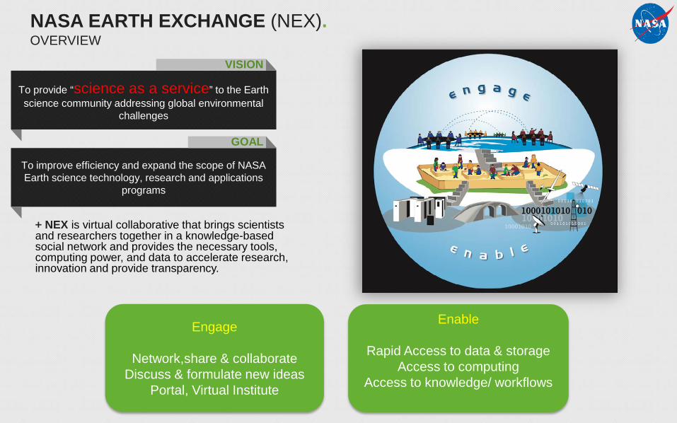
+ NEX is virtual collaborative that brings scientists and researchers together in a knowledge-based social network and provides the necessary tools, computing power, and data to accelerate research, innovation and provide transparency.

To provide “science as a service” to the Earth science community addressing global environmental

challenges

VISION

To improve efficiency and expand the scope of NASA Earth science technology, research and applications

programs

GOAL

Engage

Network,share & collaborateDiscuss & formulate new ideas

Portal, Virtual Institute

Enable

Rapid Access to data & storageAccess to computing

Access to knowledge/ workflows

NASA EARTH EXCHANGE (NEX).OVERVIEW

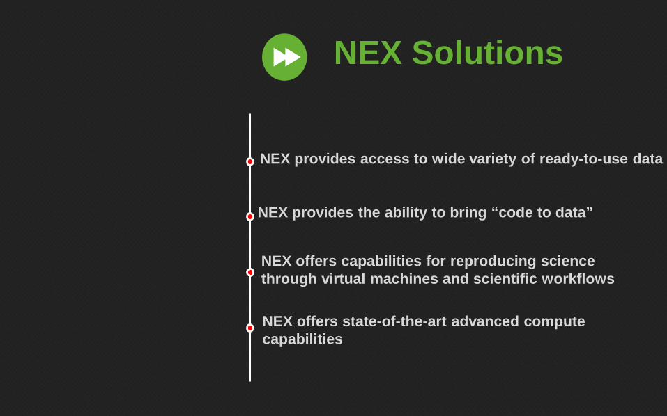
NEX Solutions

NEX provides access to wide variety of ready-to-use data

NEX provides the ability to bring “code to data”

NEX offers capabilities for reproducing science through virtual machines and scientific workflows

NEX offers state-of-the-art advanced compute capabilities

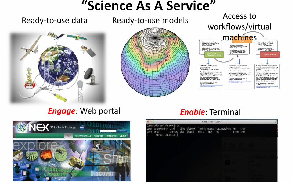
Engage: Web portal

Ready-to-use data Access to workflows/virtual

machines

Ready-to-use models

Enable: Terminal

“Science As A Service”

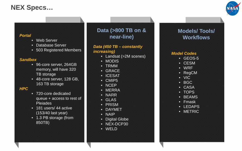
NEX Specs…

Portal• Web Server• Database Server• 503 Registered Members

Sandbox• 96-core server, 264GB

memory, will have 320 TB storage

• 48-core server, 128 GB, 163 TB storage

HPC• 720-core dedicated

queue + access to rest of Pleiades

• 181 users/ 44 active (153/40 last year)

• 1.3 PB storage (from 850TB)

Model Codes• GEOS-5• CESM• WRF• RegCM• VIC• BGC• CASA• TOPS• BEAMS• Fmask• LEDAPS• METRIC

Data (450 TB – constantly increasing)

• Landsat (>2M scenes)• MODIS• TRMM• GRACE• ICESAT• CMIP5• NCEP• MERRA• NARR• GLAS• PRISM• DAYMET• NAIP• Digital Globe• NEX-DCP30• WELD

Data (>800 TB on & near-line)

Models/ Tools/ Workflows

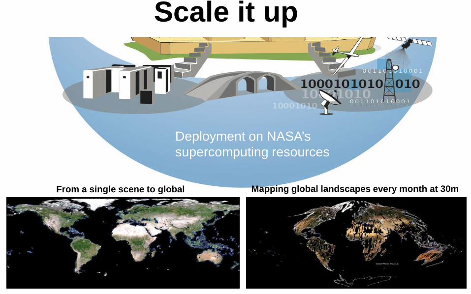
Scale it up

From a single scene to global Mapping global landscapes every month at 30m

Deployment on NASA’s supercomputing resources

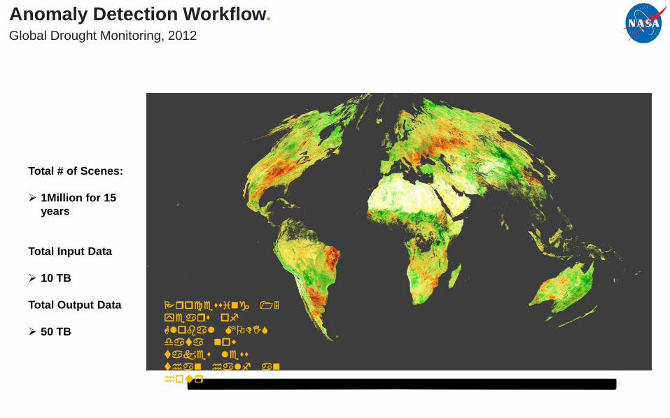
Anomaly Detection Workflow.Global Drought Monitoring, 2012

Total # of Scenes:

1Million for 15 years

Total Input Data

10 TB

Total Output Data

50 TB

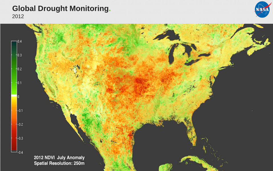
Global Drought Monitoring.2012

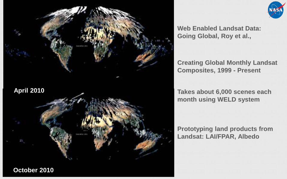
Takes about 6,000 scenes each month using WELD system

Creating Global Monthly LandsatComposites, 1999 - Present

April 2010

October 2010

Web Enabled Landsat Data: Going Global, Roy et al.,

Prototyping land products from Landsat: LAI/FPAR, Albedo

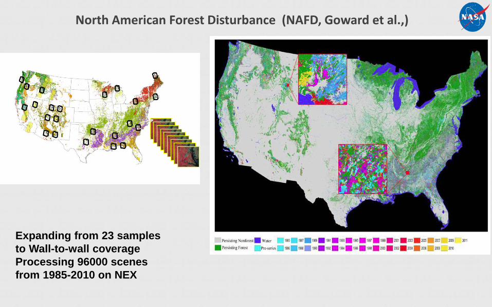
North American Forest Disturbance (NAFD, Goward et al.,)

Expanding from 23 samples to Wall-to-wall coverageProcessing 96000 scenes from 1985-2010 on NEX

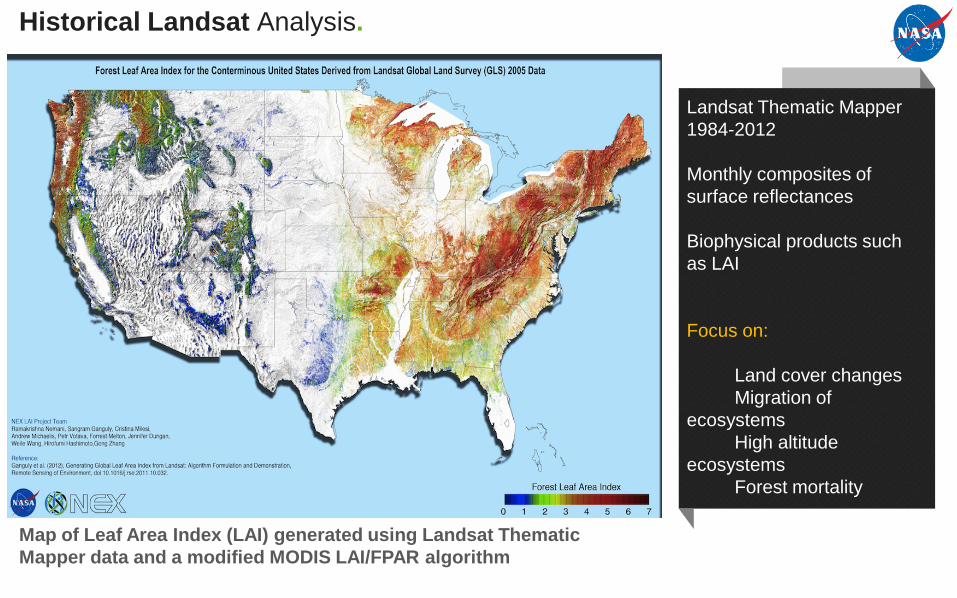
Historical Landsat Analysis.

Map of Leaf Area Index (LAI) generated using Landsat Thematic Mapper data and a modified MODIS LAI/FPAR algorithm

Landsat Thematic Mapper 1984-2012

Monthly composites of surface reflectances

Biophysical products such as LAI

Focus on:

Land cover changesMigration of

ecosystemsHigh altitude

ecosystemsForest mortality

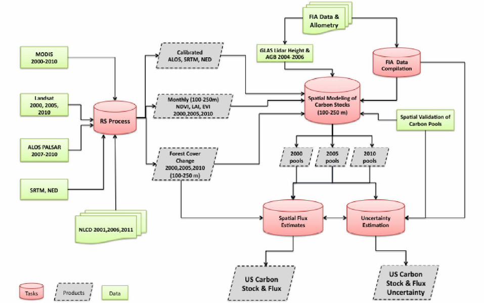
Carbon Monitoring System Phase I & II

Multi-sensor remote sensing-based estimation of Aboveground biomass

Sassan Saatchi, Sangram Ganguly, Compton Tucker, Ramakrishna Nemani, Stephen Hagen. Yifan Yu

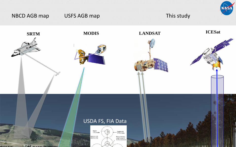
SRTM LANDSAT ICESatMODIS

USDA FS, FIA Data

NBCD AGB map USFS AGB map This study

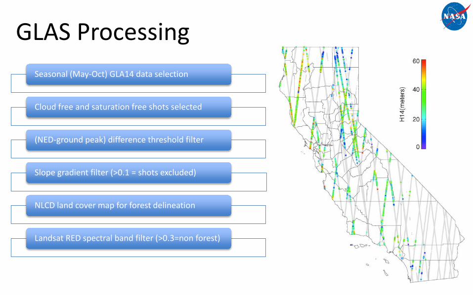
GLAS ProcessingSeasonal (May-Oct) GLA14 data selection

Cloud free and saturation free shots selected

(NED-ground peak) difference threshold filter

Slope gradient filter (>0.1 = shots excluded)

NLCD land cover map for forest delineation

Landsat RED spectral band filter (>0.3=non forest)

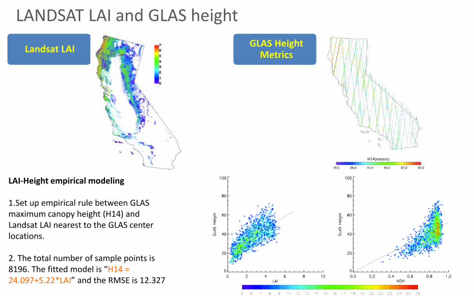
GLAS Height MetricsLandsat LAI

LAI-Height empirical modeling

1.Set up empirical rule between GLAS maximum canopy height (H14) and Landsat LAI nearest to the GLAS center locations.

2. The total number of sample points is 8196. The fitted model is “H14 = 24.097+5.22*LAI” and the RMSE is 12.327

LANDSAT LAI and GLAS height

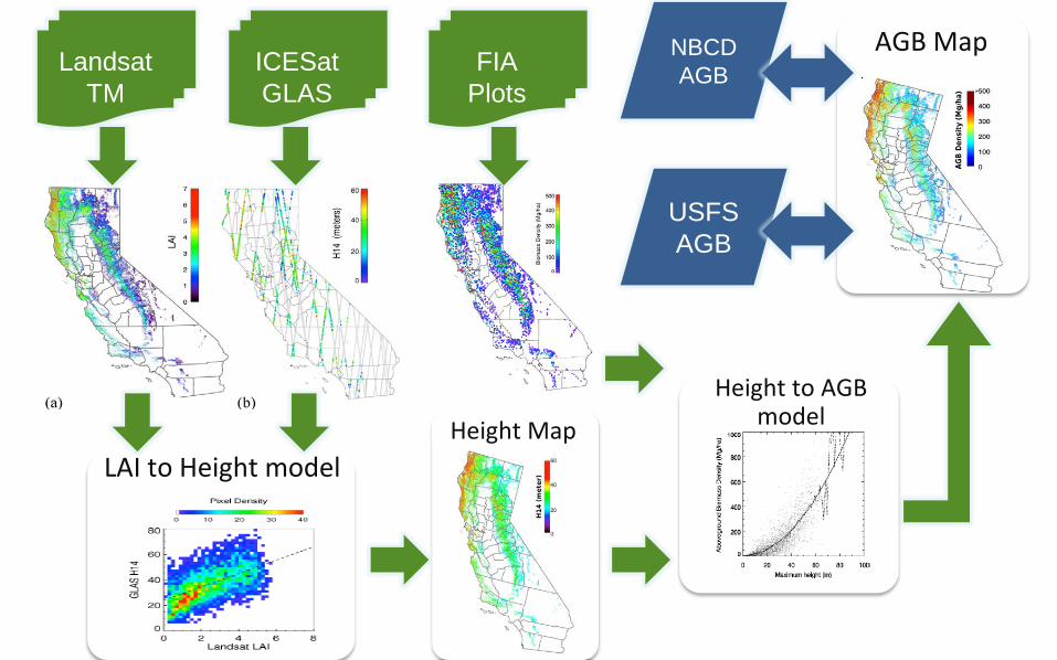
LAI to Height modelHeight Map

Height to AGB model

Landsat TM

ICESatGLAS

FIAPlots

AGB MapNBCDAGB

USFSAGB

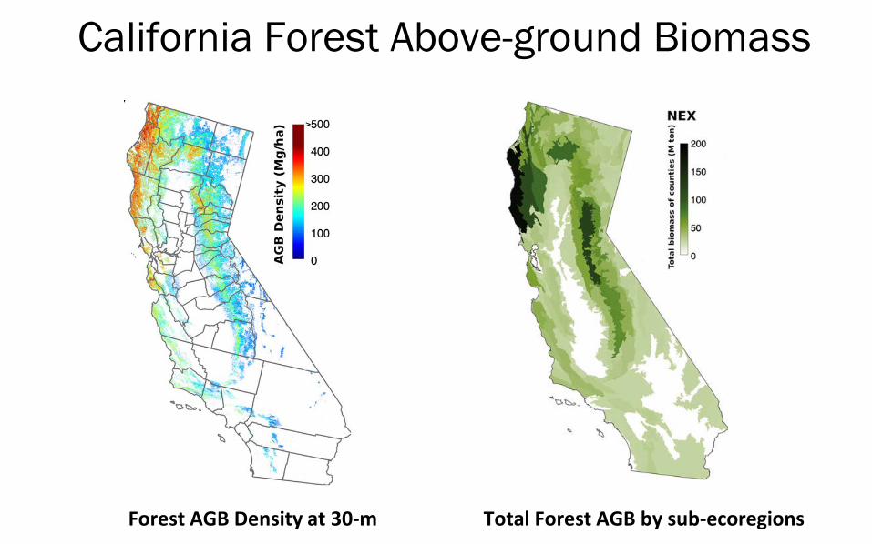
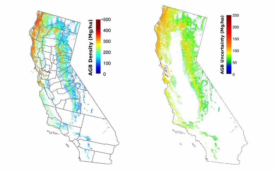
California Forest Above-ground Biomass

Forest AGB Density at 30-m Total Forest AGB by sub-ecoregions

Relative Accuracy of Total Biomass by Sub-ecoregions

Relative Accuracy of Total Biomass by Counties

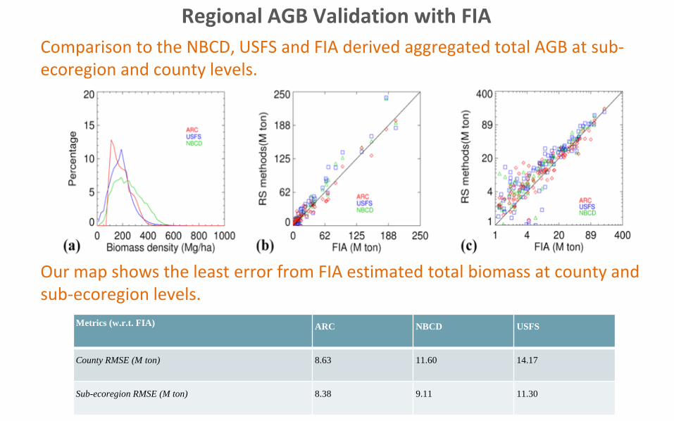
Regional AGB Validation with FIA Comparison to the NBCD, USFS and FIA derived aggregated total AGB at sub-ecoregion and county levels.

Histogram County Sub-ecoregionOur map shows the least error from FIA estimated total biomass at county and sub-ecoregion levels.

Metrics (w.r.t. FIA) ARC NBCD USFS

County RMSE (M ton) 8.63 11.60 14.17

Sub-ecoregion RMSE (M ton) 8.38 9.11 11.30

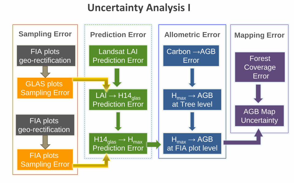
Uncertainty Analysis I

Mapping ErrorSampling Error Prediction Error Allometric Error

FIA plots Sampling Error

Landsat LAIPrediction Error

LAI → H14glasPrediction Error

Hmax → AGBat Tree level

Carbon →AGB Error

H14glas → HmaxPrediction Error

GLAS plots Sampling Error

Hmax → AGBat FIA plot level

FIA plots geo-rectification

Forest Coverage

Error

FIA plots geo-rectification

AGB MapUncertainty

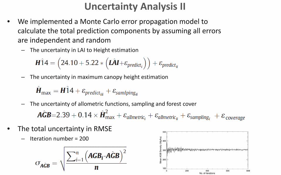
Uncertainty Analysis II• We implemented a Monte Carlo error propagation model to

calculate the total prediction components by assuming all errors are independent and random

– The uncertainty in LAI to Height estimation

– The uncertainty in maximum canopy height estimation

– The uncertainty of allometric functions, sampling and forest cover

• The total uncertainty in RMSE– Iteration number = 200

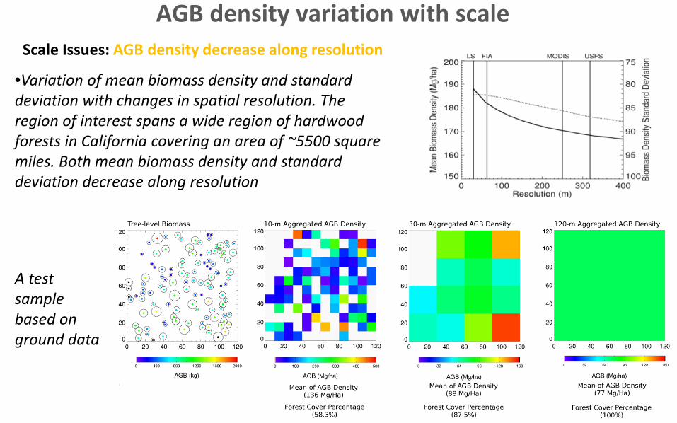
AGB density variation with scale

•Variation of mean biomass density and standard deviation with changes in spatial resolution. The region of interest spans a wide region of hardwood forests in California covering an area of ~5500 square miles. Both mean biomass density and standard deviation decrease along resolution

Scale Issues: AGB density decrease along resolution

A test sample based on ground data

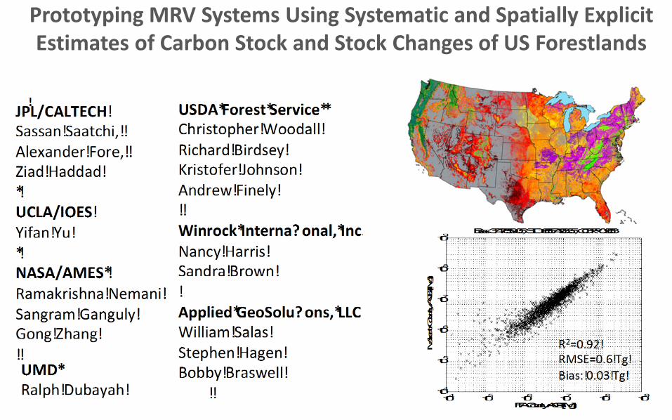
Prototyping MRV Systems Using Systematic and Spatially Explicit Estimates of Carbon Stock and Stock Changes of US Forestlands

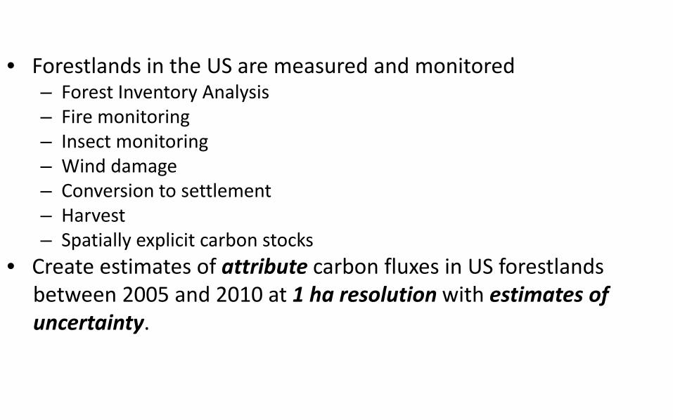
• Forestlands in the US are measured and monitored– Forest Inventory Analysis– Fire monitoring– Insect monitoring– Wind damage– Conversion to settlement – Harvest– Spatially explicit carbon stocks

• Create estimates of attribute carbon fluxes in US forestlands between 2005 and 2010 at 1 ha resolution with estimates of uncertainty.

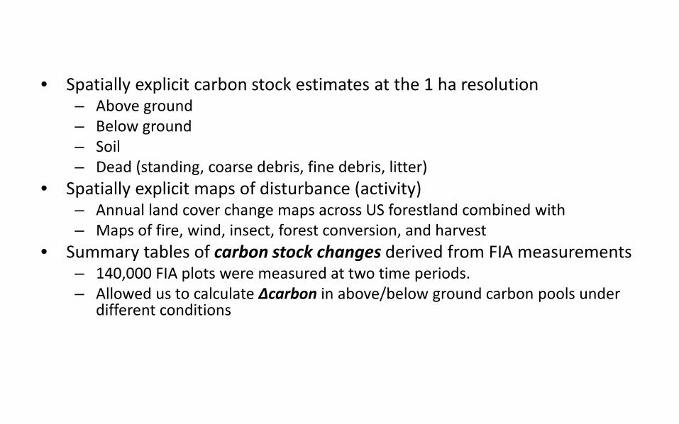
• Spatially explicit carbon stock estimates at the 1 ha resolution– Above ground– Below ground– Soil– Dead (standing, coarse debris, fine debris, litter)

• Spatially explicit maps of disturbance (activity)– Annual land cover change maps across US forestland combined with– Maps of fire, wind, insect, forest conversion, and harvest

• Summary tables of carbon stock changes derived from FIA measurements– 140,000 FIA plots were measured at two time periods.– Allowed us to calculate Δcarbon in above/below ground carbon pools under

different conditions

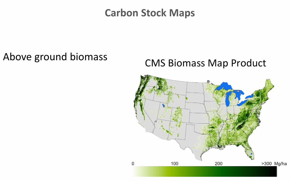
Carbon Stock Maps

Above ground biomass

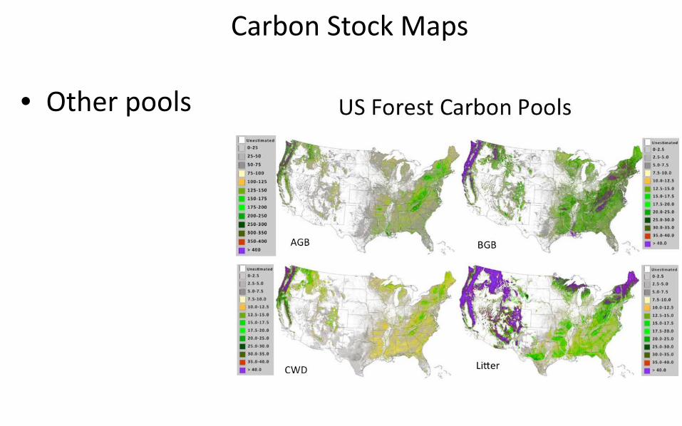
Carbon Stock Maps

• Other pools

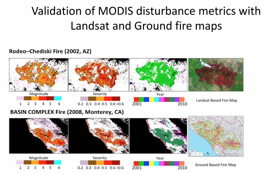
Validation of MODIS disturbance metrics with Landsat and Ground fire maps

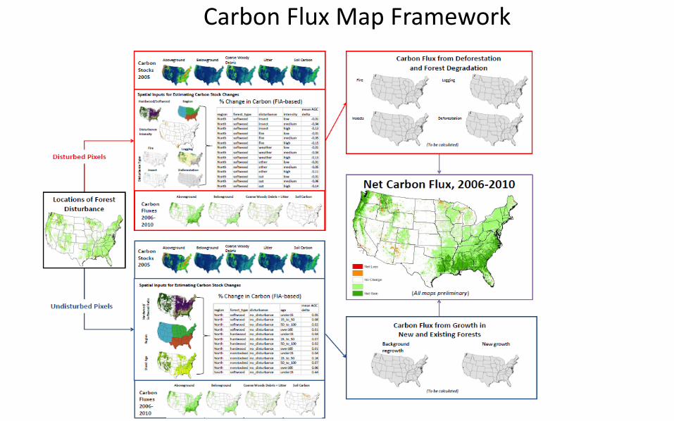
Carbon Flux Map Framework

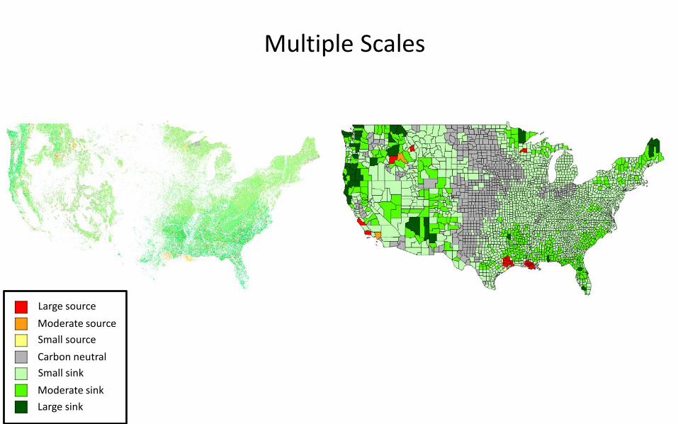
Multiple Scales

Large sourceModerate sourceSmall sourceCarbon neutral Small sinkModerate sinkLarge sink

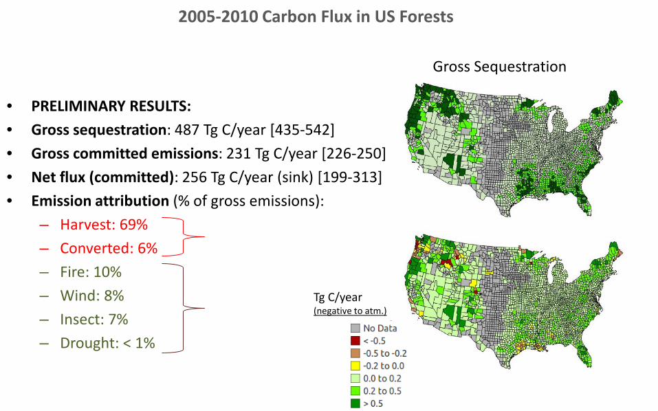
• PRELIMINARY RESULTS:• Gross sequestration: 487 Tg C/year [435-542]• Gross committed emissions: 231 Tg C/year [226-250]• Net flux (committed): 256 Tg C/year (sink) [199-313] • Emission attribution (% of gross emissions):

– Harvest: 69%– Converted: 6%– Fire: 10%– Wind: 8%– Insect: 7%– Drought: < 1%

Gross Sequestration

2005-2010 Carbon Flux in US Forests

Tg C/year(negative to atm.)

Very High Resolution Satellite Image Classification

- NASA Carbon Monitoring System (CMS) NAIP Data Application

- NASA Advanced Information Systems Technology (AIST) Program Application

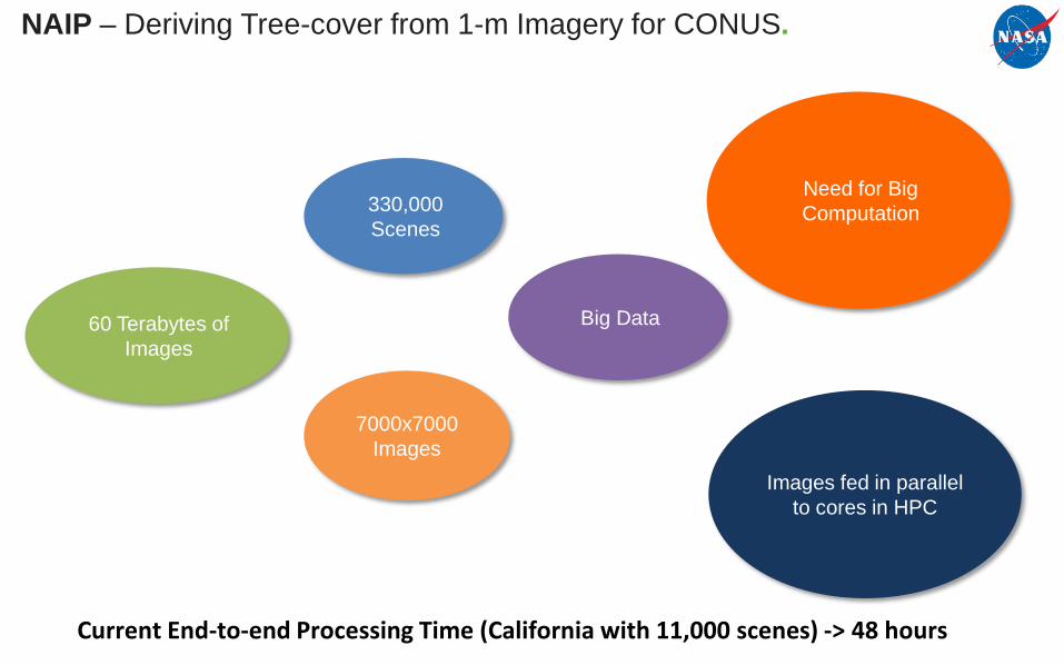
NAIP – Deriving Tree-cover from 1-m Imagery for CONUS.

330,000 Scenes

60 Terabytes of Images

7000x7000 Images

Big Data

Need for Big Computation

Images fed in parallel to cores in HPC

Current End-to-end Processing Time (California with 11,000 scenes) -> 48 hours

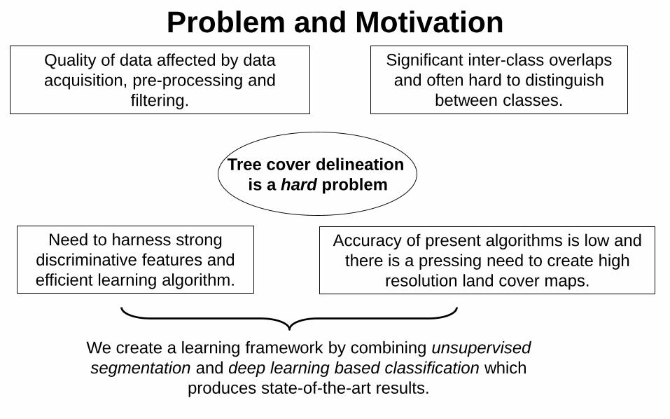
Problem and Motivation

Tree cover delineation is a hard problem

Quality of data affected by data acquisition, pre-processing and

filtering.

Significant inter-class overlaps and often hard to distinguish

between classes.

Accuracy of present algorithms is low and there is a pressing need to create high

resolution land cover maps.

Need to harness strong discriminative features and efficient learning algorithm.

We create a learning framework by combining unsupervised segmentation and deep learning based classification which

produces state-of-the-art results.

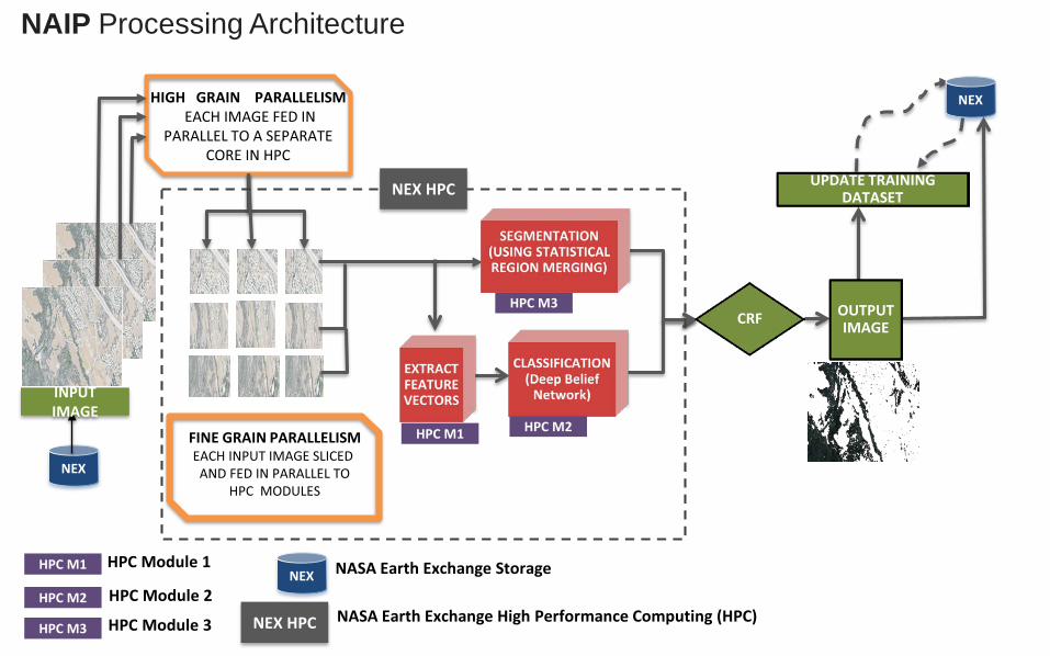
NEX

NASA Earth Exchange Storage HPC M1 HPC Module 1

HPC M2 HPC Module 2

HPC M3 HPC Module 3 NASA Earth Exchange High Performance Computing (HPC)

NEX HPC

NEX HPC

NEX

NEX

HPC M3

HPC M1 HPC M2

INPUT IMAGE

CRF

UPDATE TRAINING DATASET

OUTPUT IMAGE

NAIP Processing Architecture

nex.nasa.gov/opennex

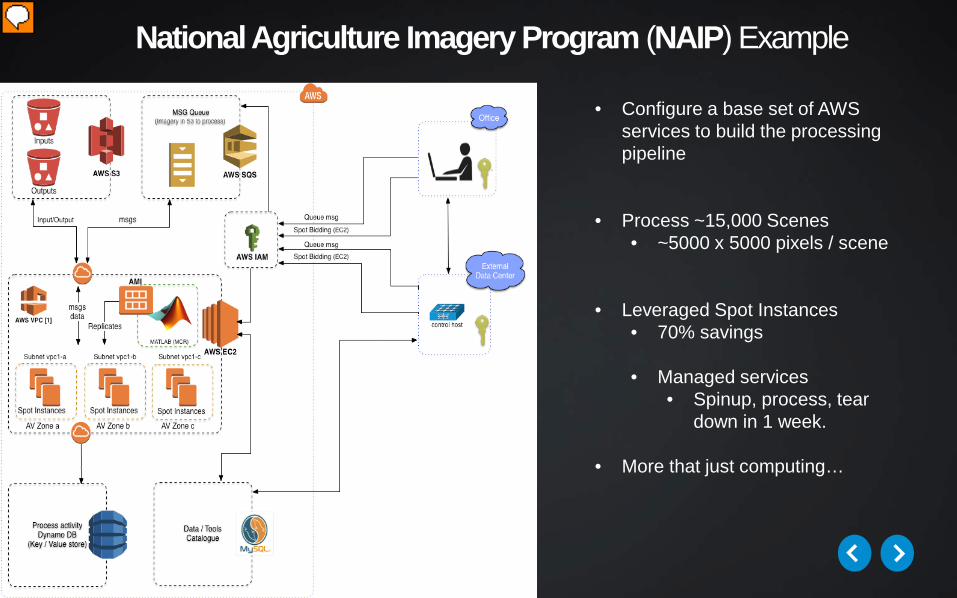
National Agriculture Imagery Program (NAIP) Example

• Configure a base set of AWS services to build the processing pipeline

• Process ~15,000 Scenes• ~5000 x 5000 pixels / scene

• Leveraged Spot Instances• 70% savings

• Managed services• Spinup, process, tear

down in 1 week.

• More that just computing…

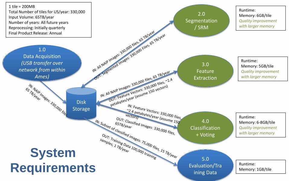
1 tile = 200MBTotal Number of tiles for US/year: 330,000Input Volume: 65TB/yearNumber of years: All future yearsReprocessing: Initially quarterlyFinal Product Release: Annual

DiskStorage

2.0Segmentation

/ SRM

3.0Feature

Extraction

4.0Classification

+ Voting

5.0Evaluation/Tra

ining Data

1.0Data Acquisition

(USB transfer over network from within

Ames)

Runtime:Memory: 6GB/tileQuality improvement with larger memory

Runtime:Memory: 5GB/tileQuality improvement with larger memory

Runtime:Memory: 6-8GB/tileQuality improvement with larger memory

Runtime:Memory: 1GB/tile

System Requirements

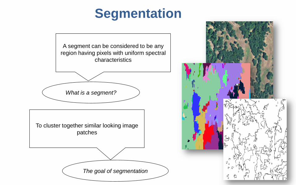
Segmentation

A segment can be considered to be any region having pixels with uniform spectral

characteristics

What is a segment?

To cluster together similar looking image patches

The goal of segmentation

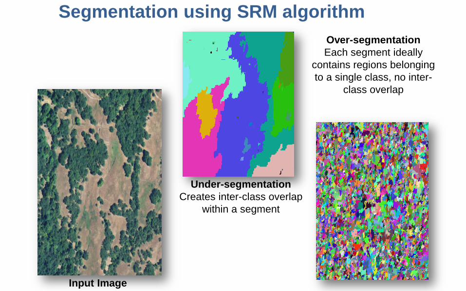
Segmentation using SRM algorithm

Under-segmentationCreates inter-class overlap

within a segment

Over-segmentationEach segment ideally

contains regions belonging to a single class, no inter-

class overlap

Input Image

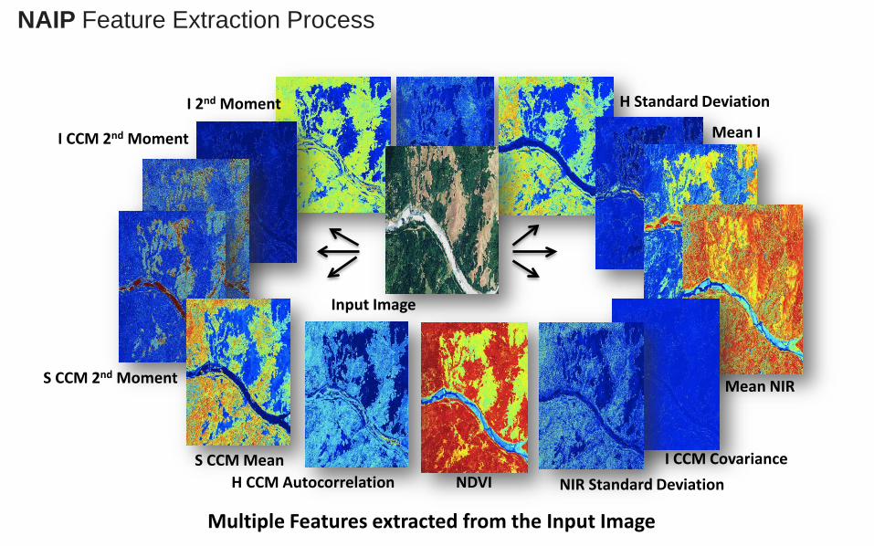
NDVI

Mean NIR

I CCM CovarianceH CCM Autocorrelation

S CCM MeanNIR Standard Deviation

S CCM 2nd Moment

I CCM 2nd Moment Mean I

I 2nd Moment H Standard Deviation

Input Image

Multiple Features extracted from the Input Image

NAIP Feature Extraction Process

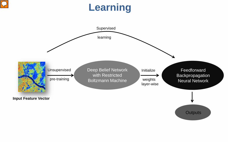
Learning

Input Feature Vector

Unsupervised

pre-training

Deep Belief Network with Restricted

Boltzmann Machine

FeedforwardBackpropagationNeural Network

Initialize

weights layer-wise

Supervised

learning

Outputs

Learning

Unsupervised Learning using Deep Belief Network: Unsupervised pre-training using a Deep Belief Network (DBN) where each

layer is trained using a Restricted Boltzmann Machine (RBM)

The weights of the DBN are used to initialize the corresponding weights of the Neural Network

A Neural Network initialized in this manner converges much faster than an otherwise uninitialized Neural Network

Unsupervised pre-training is an important step in solving a prediction problem with petabytes of data with high variability

Learning

Deep Belief Network: Each layer is conditionally independent of the other

DBN can be trained layer-wise by iteratively maximizing the conditional probability of the input vectors or visible vectors given the hidden vectors and a particular set of layer weights

A DBN trained layer-wise with RBM can help in improving the variationallower bound on the probability of the training data under the composite learning model

Learning

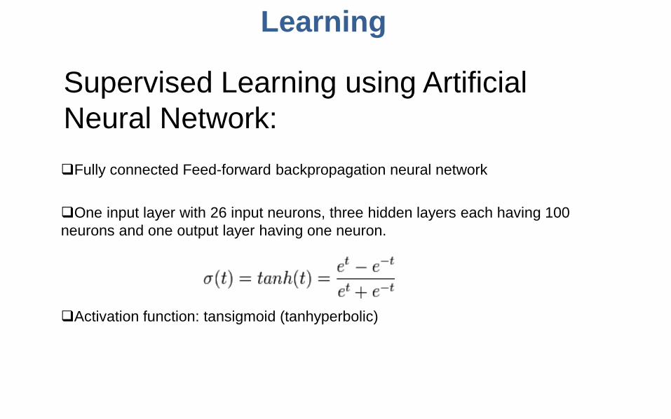
Supervised Learning using Artificial Neural Network:Fully connected Feed-forward backpropagation neural network

One input layer with 26 input neurons, three hidden layers each having 100 neurons and one output layer having one neuron.

Activation function: tansigmoid (tanhyperbolic)

Neural Network (contd.)

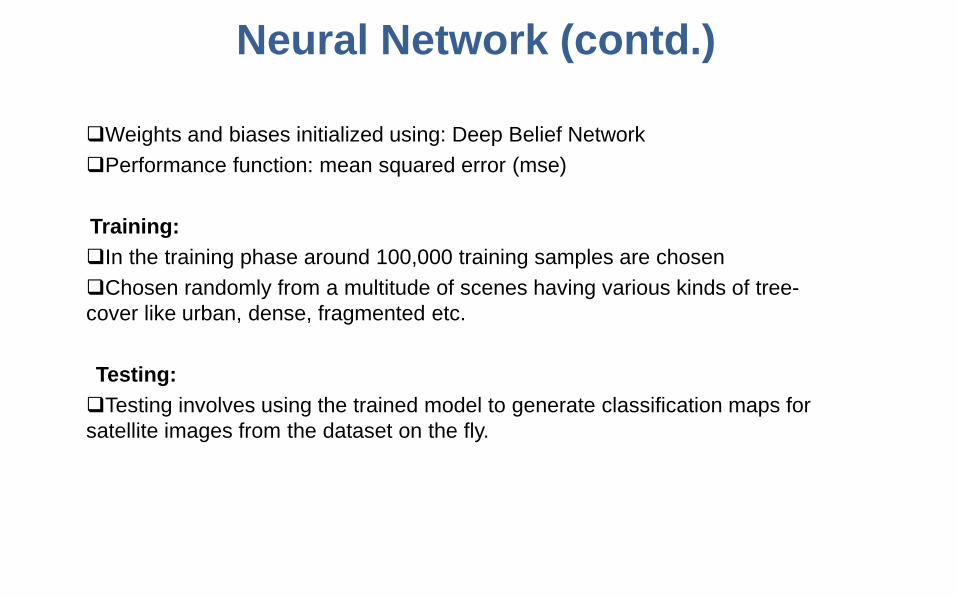
Weights and biases initialized using: Deep Belief NetworkPerformance function: mean squared error (mse)

Training:In the training phase around 100,000 training samples are chosen Chosen randomly from a multitude of scenes having various kinds of tree-cover like urban, dense, fragmented etc.

Testing:Testing involves using the trained model to generate classification maps for satellite images from the dataset on the fly.

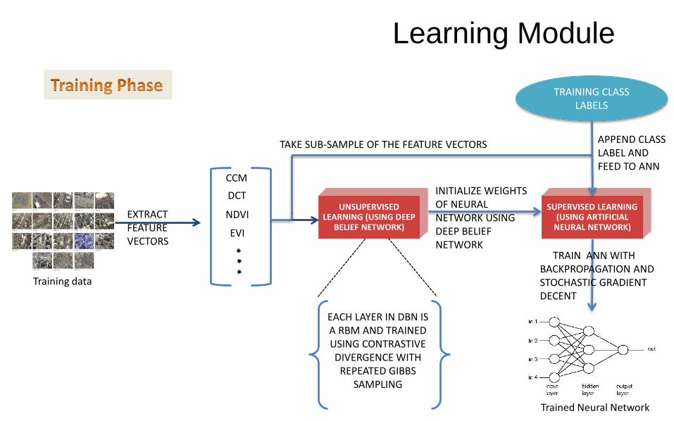
Training data

EXTRACT FEATURE VECTORS

CCMDCT

NDVI

EVI

INITIALIZE WEIGHTS OF NEURAL NETWORK USING DEEP BELIEF NETWORK

TRAINING CLASS LABELS

TAKE SUB-SAMPLE OF THE FEATURE VECTORS APPEND CLASS LABEL AND FEED TO ANN

TRAIN ANN WITHBACKPROPAGATION AND STOCHASTIC GRADIENT DECENT

Trained Neural Network

EACH LAYER IN DBN IS A RBM AND TRAINED USING CONTRASTIVE DIVERGENCE WITH

REPEATED GIBBS SAMPLING

Learning Module

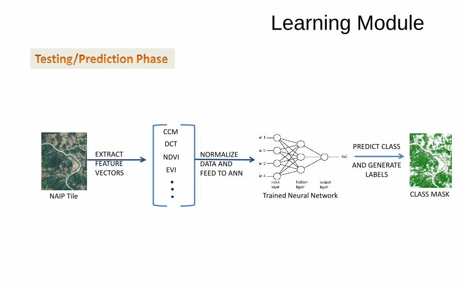
Learning Module

NAIP Tile

EXTRACT FEATURE VECTORS

CCMDCT

NDVI

EVI

Trained Neural Network CLASS MASK

PREDICT CLASS

AND GENERATELABELS

NORMALIZE DATA AND FEED TO ANN

π1

x1

π2

x2

π3

x3

π4

x4

π5

x5

π6

x6

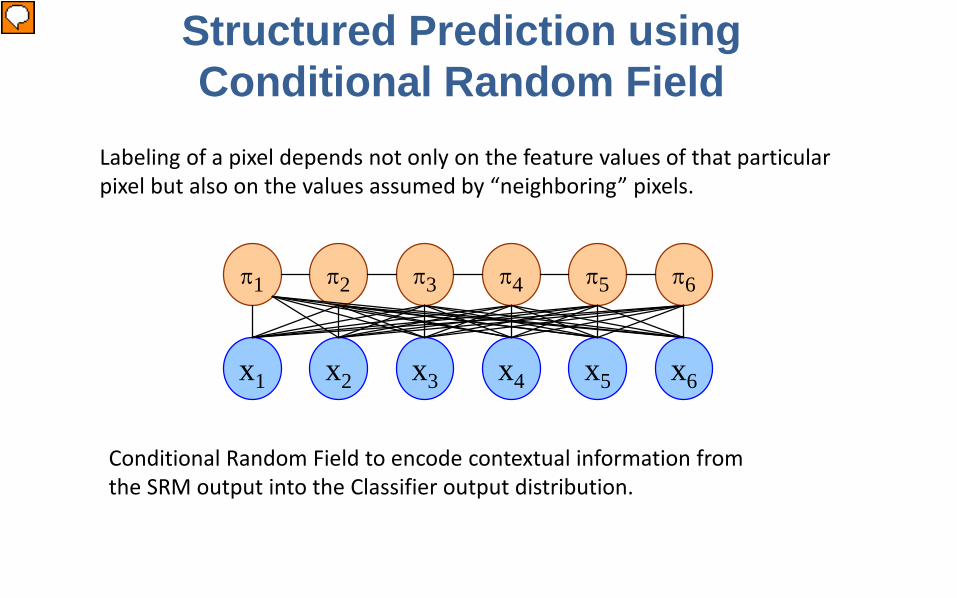
Structured Prediction using Conditional Random Field

Labeling of a pixel depends not only on the feature values of that particular pixel but also on the values assumed by “neighboring” pixels.

Conditional Random Field to encode contextual information from the SRM output into the Classifier output distribution.

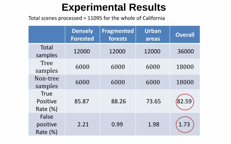
Experimental Results

DenselyForested

Fragmented forests

Urban areas Overall

Total samples 12000 12000 12000 36000

Tree samples 6000 6000 6000 18000

Non-tree samples 6000 6000 6000 18000

True Positive Rate (%)

85.87 88.26 73.65 82.59

False positiveRate (%)

2.21 0.99 1.98 1.73

Total scenes processed = 11095 for the whole of California

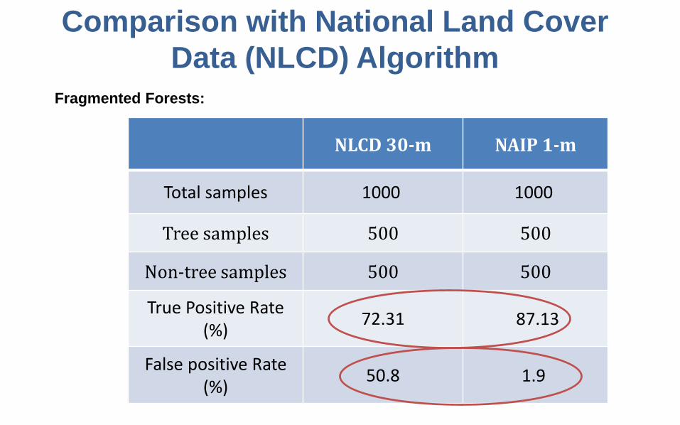
Comparison with National Land Cover Data (NLCD) Algorithm

NLCD 30-m NAIP 1-m

Total samples 1000 1000

Tree samples 500 500

Non-tree samples 500 500

True Positive Rate (%) 72.31 87.13

False positive Rate(%) 50.8 1.9

Fragmented Forests:

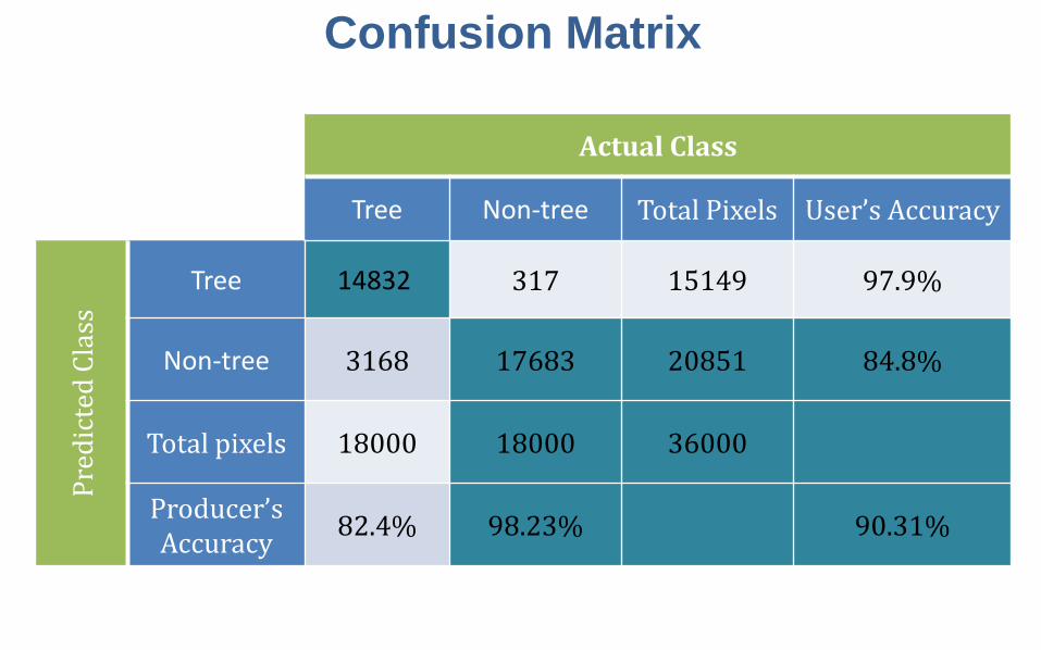
Confusion Matrix

Actual Class

Tree Non-tree Total Pixels User’s Accuracy

Pred

icte

d Cl

ass

Tree 14832 317 15149 97.9%

Non-tree 3168 17683 20851 84.8%

Total pixels 18000 18000 36000

Producer’s Accuracy 82.4% 98.23% 90.31%

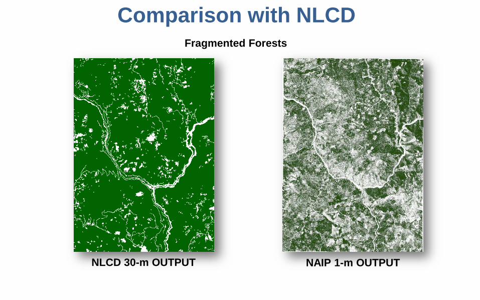
Comparison with NLCDFragmented Forests

NAIP 1-m OUTPUTNLCD 30-m OUTPUT

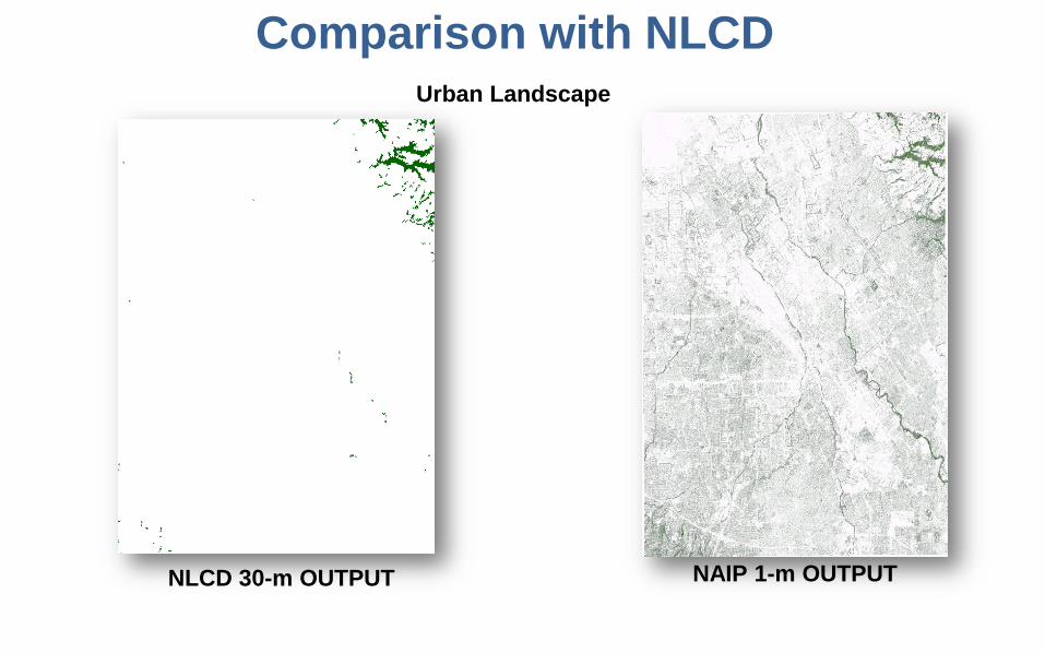
Comparison with NLCDUrban Landscape

NAIP 1-m OUTPUTNLCD 30-m OUTPUT

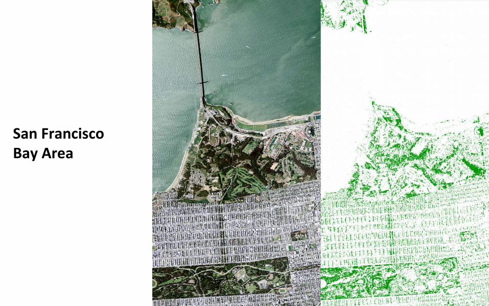
San Francisco Bay Area

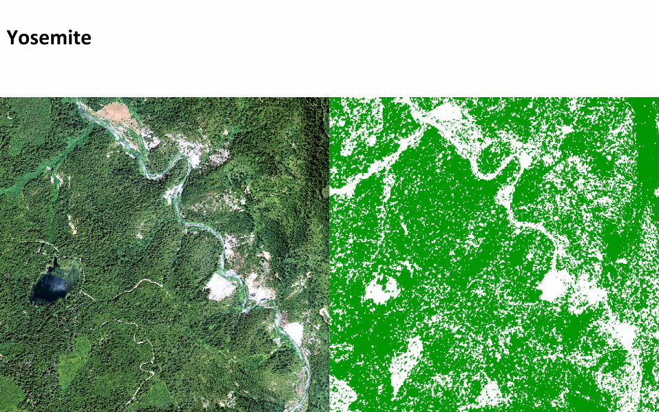
Yosemite

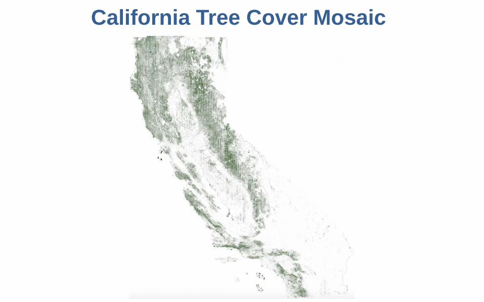
California Tree Cover Mosaic

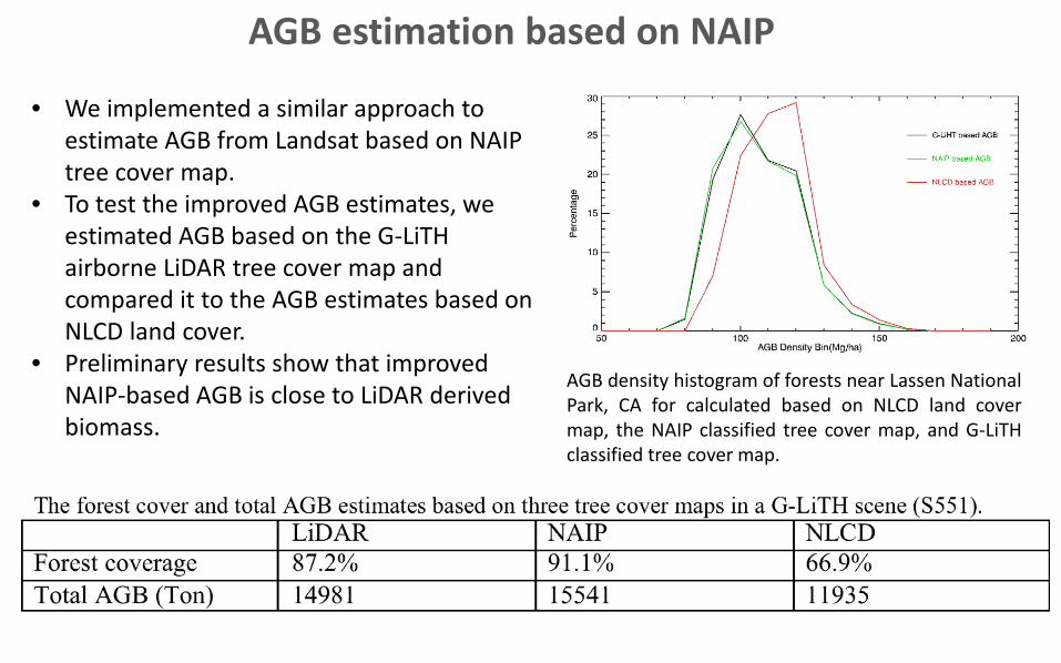
AGB estimation based on NAIP

AGB density histogram of forests near Lassen NationalPark, CA for calculated based on NLCD land covermap, the NAIP classified tree cover map, and G-LiTHclassified tree cover map.

• We implemented a similar approach to estimate AGB from Landsat based on NAIP tree cover map.

• To test the improved AGB estimates, we estimated AGB based on the G-LiTHairborne LiDAR tree cover map and compared it to the AGB estimates based on NLCD land cover.

• Preliminary results show that improved NAIP-based AGB is close to LiDAR derived biomass.

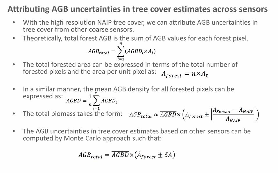
Attributing AGB uncertainties in tree cover estimates across sensors• With the high resolution NAIP tree cover, we can attribute AGB uncertainties in

tree cover from other coarse sensors. • Theoretically, total forest AGB is the sum of AGB values for each forest pixel.

• The total forested area can be expressed in terms of the total number of forested pixels and the area per unit pixel as:

• In a similar manner, the mean AGB density for all forested pixels can be expressed as:

• The total biomass takes the form:

• The AGB uncertainties in tree cover estimates based on other sensors can be computed by Monte Carlo approach such that:

Advantage of the Deep Belief Network based Learning Framework

• Since labeled training data is limited, we have to resort to UnsupervisedLearning.

• Deep Belief Networks use unlabeled data in the first phase. Since, thereare ample amounts of unlabeled data, the unsupervised learning phase isable to initialize the weights and biases of the Neural Network to a globalerror basin.

• Because the neural network is initialized to a global error basin, in thesupervised learning phase, it requires very little training data which is wellsuited for our purposes since we already have limited training data.

• DBN provides the most powerful and state-of-the-art learning frameworkto address these problems.

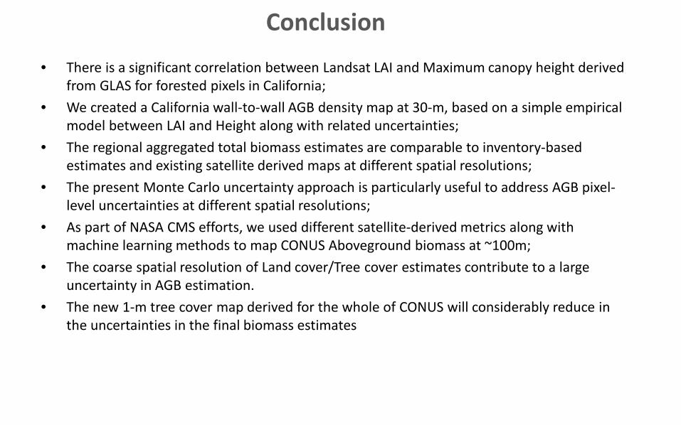
Conclusion

• There is a significant correlation between Landsat LAI and Maximum canopy height derived from GLAS for forested pixels in California;

• We created a California wall-to-wall AGB density map at 30-m, based on a simple empirical model between LAI and Height along with related uncertainties;

• The regional aggregated total biomass estimates are comparable to inventory-based estimates and existing satellite derived maps at different spatial resolutions;

• The present Monte Carlo uncertainty approach is particularly useful to address AGB pixel-level uncertainties at different spatial resolutions;

• As part of NASA CMS efforts, we used different satellite-derived metrics along with machine learning methods to map CONUS Aboveground biomass at ~100m;

• The coarse spatial resolution of Land cover/Tree cover estimates contribute to a large uncertainty in AGB estimation.

• The new 1-m tree cover map derived for the whole of CONUS will considerably reduce in the uncertainties in the final biomass estimates

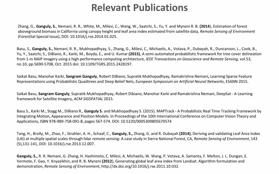
Relevant PublicationsZhang, G., Ganguly, S., Nemani, R. R., White, M., Milesi, C., Wang, W., Saatchi, S., Yu, Y. and Myneni R. B. (2014), Estimation of forest aboveground biomass in California using canopy height and leaf area index estimated from satellite data, Remote Sensing of Environment (ForestSat Special Issue), DOI: 10.1016/j.rse.2014.01.025.

Basu, S., Ganguly, S., Nemani, R. R., Mukhopadhyay, S., Zhang, G., Milesi, C., Michaelis, A., Votava, P., Dubayah, R., Duncanson, L., Cook, B., Yu, Y., Saatchi, S., DiBiano, R., Karki, M., Boyda, E., and U. Kumar (2015), A semi-automated probabilistic framework for tree cover delineation from 1-m NAIP imagery using a high performance computing architecture, IEEE Transactions on Geoscience and Remote Sensing, vol.53, no.10, pp.5690-5708, Oct. 2015 doi: 10.1109/TGRS.2015.2428197.

Saikat Basu, Manohar Karki, Sangram Ganguly, Robert DiBiano, Supratik Mukhopadhyay, Ramakrishna Nemani, Learning Sparse Feature Representations using Probabilistic Quadtrees and Deep Belief Nets, European Symposium on Artificial Neural Networks, ESANN 2015.

Saikat Basu, Sangram Ganguly, Supratik Mukhopadhyay, Robert Dibiano, Manohar Karki and Ramakrishna Nemani, DeepSat - A Learning framework for Satellite Imagery, ACM SIGSPATIAL 2015.

Basu S., Karki M., Stagg M., DiBiano R., Ganguly S. and Mukhopadhyay S. (2015). MAPTrack - A Probabilistic Real Time Tracking Framework by Integrating Motion, Appearance and Position Models. In Proceedings of the 10th International Conference on Computer Vision Theory and Applications, ISBN 978-989-758-091-8, pages 567-574. DOI: 10.5220/0005309805670574

Tang, H., Brolly, M., Zhao, F., Strahler, A. H., Schaaf, C., Ganguly, S., Zhang, G. and R. Dubayah (2014), Deriving and validating Leaf Area Index (LAI) at multiple spatial scales through lidar remote sensing: A case study in Sierra National Forest, CA, Remote Sensing of Environment, 143 (5),131-141, DOI: 10.1016/j.rse.2013.12.007.

Ganguly, S., R. R. Nemani, G. Zhang, H. Hashimoto, C. Milesi, A. Michaelis, W. Wang, P. Votava, A. Samanta, F. Melton, J. L. Dungan, E. Vermote, F. Gao, Y. Knyazikhin, and R. B. Myneni (2012), Generating global leaf area index from Landsat: Algorithm formulation and demonstration, Remote Sensing of Environment, http://dx.doi.org/10.1016/j.rse.2011.10.032.

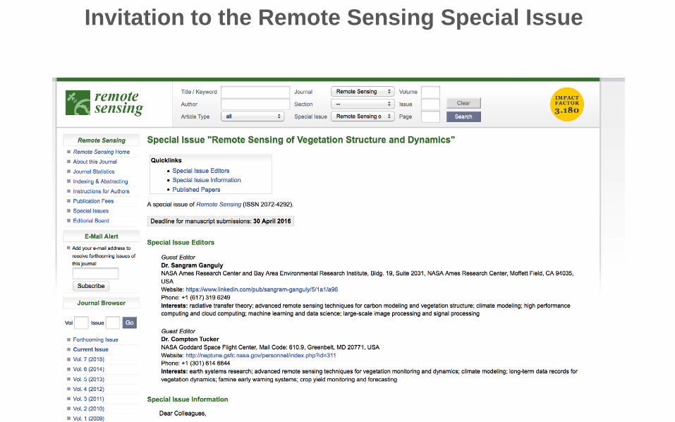
SummaryInvitation to the Remote Sensing Special Issue

FOR YOUR ATTENTION

exit

THANKYOU.