Biomass from Crop Residues: Cost and Supply Estimates.

Biomass from Crop Residues: Cost and Supply Estimates. by Paul Gallagher,Mark Dikeman, John Fritz, Eric Wailes, Wayne Gauther, and Hosein Shapouri.U.S. Department of Agriculture, Office of the Chief Economist, Office of EnergyPolicy and New Uses. Agricultural Economic Report No. 819

Abstract

The supply of harvested crop residues as a feed stock for energy products is esti-mated in this report. The estimates account for economic and environmentalfactors governing residue supply. The supply results span major agricultural cropsin four distinct cropping regions of the United States, taking into account localvariation in cost-determining factors such as residue yield, geographic density ofresidues, and competition for livestock feed use.

Keywords: Crop residues, harvested residue, residue yield, supply estimates, soilquality, cropping regions, feedstock, biomass technologies, reduced tillage, forage.

About the Authors

Paul Gallaghner is in the Economics Department at Iowa State University,Mark Dikeman was in the Animal Science Department at Iowa State University,John Fritz is in the Agronomy Department at Kansas State University, EricWailes is in the Agricultural Economics Department at the University ofArkansas, Wayne Gauther is in the Agricultural Economics Department atLouisiana State University, and Hosein Shapouri is in the Office of EnergyPolicy and New Uses, USDA.

Acknowledgments

The authors thank Thomas McDonald and Dana Rayl West for the excellenteditorial assistance, Wynnice Pointer-Napper for the final document layout,charts, and cover design.

300 7th Street, SWRoom 361 Reporters BuildingWashington, DC 20024 February 2003

ii � Biomass from Crop Residues: Cost and Supply Estimates / AER-819 Office of Energy Policy and New Uses

Contents

Summary . . . . . . . . . . . . . . . . . . . . . . . . . . . . . . . . . . . . . . . . . . . . . . . . . . . . . . . iii

Introduction . . . . . . . . . . . . . . . . . . . . . . . . . . . . . . . . . . . . . . . . . . . . . . . . . . . . . 1

Farm Supply Function for Crop Residues: General Comments . . . . . . . . . . . . 1

Estimation Procedures . . . . . . . . . . . . . . . . . . . . . . . . . . . . . . . . . . . . . . . . . . . . . 2

Supply Areas, Transport, and Input Costs for Processing Plants . . . . . . . . . . . . 3

Multiple Supplies and Input Costs . . . . . . . . . . . . . . . . . . . . . . . . . . . . . . . . . . . 4

Regions . . . . . . . . . . . . . . . . . . . . . . . . . . . . . . . . . . . . . . . . . . . . . . . . . . . . . . . . 5

Environmental Constraints . . . . . . . . . . . . . . . . . . . . . . . . . . . . . . . . . . . . . . . . . 6

A Harvest Cost Function . . . . . . . . . . . . . . . . . . . . . . . . . . . . . . . . . . . . . . . . . . . 8

Cost Estimates . . . . . . . . . . . . . . . . . . . . . . . . . . . . . . . . . . . . . . . . . . . . . . . . . . . 10

Feed Values Estimates . . . . . . . . . . . . . . . . . . . . . . . . . . . . . . . . . . . . . . . . . . . . . 10

Supply Curves . . . . . . . . . . . . . . . . . . . . . . . . . . . . . . . . . . . . . . . . . . . . . . . . . . . 11

Biomass Supply and Capacity . . . . . . . . . . . . . . . . . . . . . . . . . . . . . . . . . . . . . . 13

Summary and Conclusions . . . . . . . . . . . . . . . . . . . . . . . . . . . . . . . . . . . . . . . . . 14

References . . . . . . . . . . . . . . . . . . . . . . . . . . . . . . . . . . . . . . . . . . . . . . . . . . . . . . 15

Appendix Tables A - Costs . . . . . . . . . . . . . . . . . . . . . . . . . . . . . . . . . . . . . . . . . 17

Appendix Tables B - Quantity . . . . . . . . . . . . . . . . . . . . . . . . . . . . . . . . . . . . . . 22

Glossary . . . . . . . . . . . . . . . . . . . . . . . . . . . . . . . . . . . . . . . . . . . . . . . . . . . . . . . . 26

Office of Energy Policy and New Uses Biomass from Crop Residues: Cost and Supply Estimates / AER-819 � iii

Summary

Biomass supply from crop residues can increase producer profits while main-taining soil quality, provided that reduced tillage and partial residue harvest are used appropriately. Corn Belt, Great Plains, and West Coast participation is possible with judicious selection of crops and management practices. Also,residues are probably the lowest cost form of biomass supply, but the range ofcosts is wider in the Great Plains than in the Corn Belt. The remaining regions, theWest Coast, the Delta, and the Southeast, also have pockets with residue suppliesand a wide variation in costs.

Crop residues have the potential to displace 12.5 percent of petroleum imports or 5 percent of electricity consumption in today’s markets. Residues also havegrowth potential from improving crop productivity and declining livestockdemands for forage. When residue supplies are included with some other agricul-tural sources, biomass supply from crop agriculture could account for an impor-tant share of our energy consumption. But further development of processingtechnology is still needed.

Office of Energy Policy and New Uses Biomass from Crop Residues: Cost and Supply Estimates / AER-819 � 1

Introduction

Harvested residues from annual field crops are suit-able as a feedstock for some emerging industrial

processes, such as the production of ethanol and plas-tics (Committee on Biobased Industrial Products,2000). Some estimates suggest that crop residue quan-tities compare favorably with wood residues (Spelman,1994); however, the economic and environmentalfactors governing residue supply have not been evalu-ated. The supply estimates presented here span majoragricultural crops in four distinct cropping regions ofthe United States, taking into account local variation in cost-determining factors such as residue yield,geographic density of residues, and competition forlivestock feed use. Specifically, residues are includedin the estimation of potential industrial supply only iftheir removal by harvest would not result in excessivesoil erosion. This is a necessary restriction becausefarmers’ decisions and government policies will likelybe consistent with soil conservation.

Subsequent sections of the paper look at the residuesupply curves for major crops. First, estimation proce-dures and environmental constraints are reviewed. Thencost and supply estimates are presented for the majorcrop-producing regions of the United States. Theresults suggest that crop residues will be able toprovide a moderate amount of the U.S. fuel supply withthe advent of fully developed biomass technologies.

Farm Supply Function for Crop Residues: General Comments

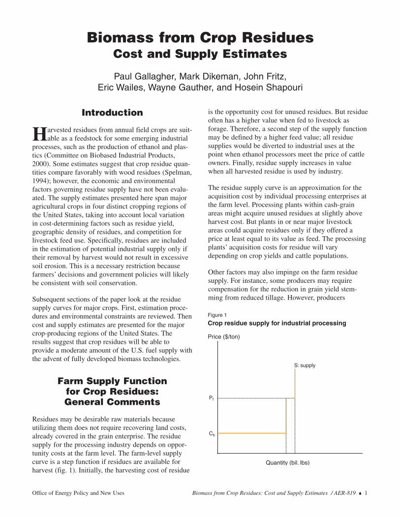
Residues may be desirable raw materials becauseutilizing them does not require recovering land costs,already covered in the grain enterprise. The residuesupply for the processing industry depends on oppor-tunity costs at the farm level. The farm-level supplycurve is a step function if residues are available forharvest (fig. 1). Initially, the harvesting cost of residue

is the opportunity cost for unused residues. But residueoften has a higher value when fed to livestock asforage. Therefore, a second step of the supply functionmay be defined by a higher feed value; all residuesupplies would be diverted to industrial uses at thepoint when ethanol processors meet the price of cattleowners. Finally, residue supply increases in valuewhen all harvested residue is used by industry.

The residue supply curve is an approximation for theacquisition cost by individual processing enterprises atthe farm level. Processing plants within cash-grainareas might acquire unused residues at slightly aboveharvest cost. But plants in or near major livestockareas could acquire residues only if they offered aprice at least equal to its value as feed. The processingplants’ acquisition costs for residue will varydepending on crop yields and cattle populations.

Other factors may also impinge on the farm residuesupply. For instance, some producers may requirecompensation for the reduction in grain yield stem-ming from reduced tillage. However, producers

Biomass from Crop ResiduesCost and Supply Estimates

Paul Gallagher, Mark Dikeman, John Fritz, Eric Wailes, Wayne Gauther, and Hosein Shapouri

Figure 1

Crop residue supply for industrial processing

Price ($/ton)

Quantity (bil. lbs)

S: supply

Ch

Pf

2 � Biomass from Crop Residues: Cost and Supply Estimates / AER-819 Office of Energy Policy and New Uses

without erosion problems will remain beyond theconservation margin with conventional tillage. Residueharvest in northern climates may require more harvestcapital and timely labor supply due to the short harvestseason. Elsewhere, harvesting capital requirements andcosts may be lower if harvesting continues through thewinter and processors provide harvesting services. Inthese situations, the harvesting capacity could matchthe monthly capacity of the processing plant.

Estimation Procedures

The usual econometric tools are not useful for esti-mating the supply of residues because substantialmarkets for these products do not yet exist. Specifically,there are no output and price data. Entry-point supplyestimates are appropriate because the level of producerparticipation in residue harvest is the main supplyadjustment. Individual firms or local supply areas aresorted with low-cost producers first and high-costproducers last. The capacity that corresponds to a partic-ular entry price is included in supply when costs arecovered. Elsewhere, entry-point supply analysis is usedto analyze transport services in international trade(Shimojo, 1979) and for producer participation deci-sions in government programs in agriculture (Hoag andHolloway, 1991; Perry et al., 1989).

Two types of economic information are developed foreach producer or local supply area. First, the height ofthe local supply function is analyzed with cost calcula-tions. Second, a residue balance sheet identifies theoutput available at the cost threshold. Firms or groupsof firms with particular types of outputs are ranked fromlow cost to high cost. All cost, output, and feed esti-mates are developed using county data, since agronomicconditions are uniform at this level. Data from 1997 areused for the baseline because the most recent Census ofAgriculture supplements the annual data from the U.S.Department of Agriculture. County data are used touncover the effects of variation in residue yield, density,and forage requirements on cost and supply.

Costs. Several costs determine the height of the farmsupply curve for crop residues. First, the cost ofharvesting residue is the opportunity cost of residue incash grain areas. Cost estimates for chopping, baling,and on-farm hauling of crop residues are included.Because unused residues may have value (in that they

reduce fertilizer needs or soil erosion), appropriateadjustments are included in cost estimates. Second, theresidue market will reflect the forage value of residueand prices for the close substitute, hay, when the unusedresidue is exhausted in a local area. Quality discountsfrom the hay price are typical, and the extent ofdiscounting depends on the type of residue. Third, thetransport rate and density of available residues influencethe costs of assembly and delivery to the plant.

Supply and Utilization Tables for Residues. Theindustrial supply of residue available at harvest cost isestimated by residue production, less forage demand.The residue used for forage is also available to indus-trial processors at prices above the forage value.

The residue production calculation is straightforwardmultiplication of area and yield. But environmentalfactors account for three types of supply restrictions:reducing yield, eliminating land from residue harvest,and using reduced tillage. The marginal land and agro-nomic practices for residue harvest are identified byevaluating erosion-residue harvest tradeoffs with repre-sentative soils and alternative production methods, asdescribed in subsequent sections. Yield reductionsassociated with government conservation requirementsor conservation tillage are also explained later.

Forage demand estimates at the local county level takeinto account cattle population, the daily forage require-ments of various types of cattle, and the local avail-ability of forage supplied by pasture. The daily foragerequirements of various types of cattle are shown intable 1. These feed requirements are taken from theCommittee on Beef Cattle Nutrition (1996) andJurgens. The length of the grazing season is estimatedat the State level (table 1b). The estimated growingseason is defined when rapid growth degree day accu-mulations begin and end. The annual cattle foragedemand is the annualized daily feed requirement,excluding the proportion of the year that cowspasture.1

Local hay and silage production is subtracted from theannual forage demand. The forage requirement not takeninto account approximates residue demand by cattle.

1 The details of pasture season length estimation and feed require-ments by type of cow are discussed in a separate report, availablefrom the author upon request.


Supply Areas, Transport, and Input Costs for Processing Plants

The main factors influencing the spread between farmcosts and delivered plant costs are the density ofresidue, the capacity of processing plants, and localtruck-hauling rates. It is important to account for localvariation in transport costs. Otherwise, an area withsparse supplies of very low-cost residues might bemistaken for a low-cost region. Or an area withmoderate yield and harvest cost but dense supplies

might be excluded, mistakenly, from potential plantlocations with low-cost biomass.

The transportation component of material costsincreases with factory capacity because greaterdistances are traveled to secure supplies. The physicalrelationship between distance from the plant (r) andavailable supplies (Q) from one crop can be approxi-mated by:

Q = (πr2)dy,

which is the product of the area of a circle of radius r,πr2, and the density of residue, dy. In turn, residuedensity is the product of residue yield (y) and thedensity of planted crops in the total area (d). Forexample, d=320 acres of residues/mi2 in a county withhalf of the land in corn and maybe y=3 tons ofresidue/acre, giving a volume density of dy=960ton/mi2.

When Q is set at the capacity of the processing plant,the maximum distance required by the plant can beobtained by rearranging

For the cost-distance relationship, notice that theproduction obtained from a ring of a given distancefrom the plant is given by the product of the circumfer-ence of the circle, the width of the ring, and the densityof residue ∆Q = (2πr)(dy)∆r. The marginal cost ofexpanding the outer circle by the increment ∆r is givenby C′(r) = P(r)(2πr)(dy)∆r. P(r) is the price gradientfunction describing the price-distance surface—in awell-chosen location, the price gradient should be thesum of residue harvest and transport costs. With a linearprice gradient, the total cost function

becomes

where t is transport cost in $/ton/mile. The averageinput cost (AIC) is

Table 1—Cattle forage requirements by type of cattle

Type Daily forage requirement

Pounds/day

Beef cows 27.6Milk cows 25.2Beef replacement heifers 13.2Milk replacement heifers 9.6Bulls over 500 lbs. 30.0Steers 5.8Heifers 5.5

~

( ).dy/Q~

*r π=

∫ π= r0 r)(dy)drP(r)(2* C(r)

,*r3

t2P)dy)(r(rdr)trP( o

2*

0o ⎥⎦

⎤⎢⎣⎡ +π=+∫π=

*r

)(dy)(2 C(r)

.3

*tr2P

*)r(Q

*)r(C0 +=

Table 1b—Length of grazing season, by State

State No. days in grazing season

Arkansas 224California 241Colorado 153Illinois 156Indiana 154Iowa 146Kansas 175Louisiana 257Michigan 142Minnesota 138Mississippi 225Missouri 185Montana 160Nebraska 157North Dakota 137Ohio 157Oklahoma 202Oregon 161South Dakota 143Texas 221Washington 161Wisconsin 136Wyoming 140


Hence, the spread between AIC and farm costs, 2tr*/3,increases with the transport rate and the maximumdistance. In turn, the supply radius increases with plantcapacity and declines with greater supply densities.

Multiple Supplies and Input Costs

When there are several different types of crop residuesin an area, the farm supply function for crop residueswould likely have several steps corresponding to theresidue supplies of a particular crop. Residue costsvary from crop- to- crop because the yield and theopportunity values for fertilizer replacement aredifferent. This section considers the determination ofefficient supply areas when there are several types ofcrop residues.

Suppose P0i is the harvest cost for crop residue i. Also,ri is the radius of the supply area for crop i. Alsoassume that crop 1 has lowest harvest costs, crop 2 issecond-lowest, and so on. A processor seeking theminimum cost input will expand the supply area sothat the cost of marginal supply is equal for each typeof residue. The conditions

identify the boundaries of supply area 2 and supplyarea 3 (r2 and r3) when the boundary of 1 (r1) is givenin the three-product case.

To determine the market areas for each type of residue,notice that capacity output must equal the sum ofproduction from each residue type

When there are three supply areas with radii r1 , r2 ,and r3, equations 1 and 2 above provide a set of threeequations that can be solved for the radii of the marketareas. The equations in 1 can be substituted into 2 toeliminate r2 and r3. Then the quadratic formula can beused to solve for the radius r1 that has efficient bound-aries and fills the plant capacity.

The case when higher cost residues are not used canbe identified without recourse to Kuhn-Tucker condi-tions. For instance, the market border condition,

P01 + r1 t = P02 + r2 t ,

also identifies the utilization threshold for the second(or third) crop. Specifically,

P01 + r1 t = P02 when r2 = 0.

Generally, the supply radius for crop i when crop j ison the entry threshold (Rij) is

R12 = ( P02 - P01 ) / t

R13 = ( P03 - P01 ) / t

R23 = ( P03 - P02 ) / t .

Next, we can check whether the plant’s capacity hasbeen filled by the time an entry threshold is reached.First, calculate the outputs associated with the two-product and three-product boundaries

All three possible cases can be defined with entrypoints and associated outputs. First, a plant’s capacityis filled with one crop before the second crop is used ifQ2 > Q. Further, a two-product supply area fillscapacity if Q2 < Q < Q3. Finally, a three-productsupply area is used if Q3 < Q.

Equipped with a list of included crops and supply areas(r1, r2, r3), the plant’s residue costs can be defined.Specifically, the total costs of residue type i are

with linear transport costs. Also, the output producedusing residues of type i are

Finally, the average input costs are defined by

So average input costs depend on the average harvestcosts and transport charges,

ii2i

iydr Q Π∑= (2).

2222311

2132

112122

ydRydRQydRQ

+Π=Π=

⎥⎦⎤

⎢⎣⎡ +Π= i01ii

2ii tr

3

2P)yd)(r( )C(r

ii2ii ydr Q Π=

.Q

)C(r AIC

i

ii

∑

∑=

Q /QS, rS

r ,PSPwhere rt3/2PAIC

iiiii

i

i0i

i00

∑=∑

=∑=+=

trPtrP

trPtrP

303101

202101

+=++=+

(1)


when several crops provide residue supplies, where Sirefers to the share of supply provided by crop residue i.

Regions

The regions of this study are areas with high-densityproduction of a major crop that share common agro-nomic practices. County-level definitions of regionsare used because only parts of most States should beincluded. County data also help to uncover the extentof variation in production costs. The four regionsdefined in figure 2 are the Corn Belt, the Great Plains,the West Coast, and the South.

The Corn Belt includes eastern Nebraska, southernMinnesota, Iowa, southern Wisconsin, Illinois, Indiana,southern Michigan, and eastern Ohio. The dominantcrop choices in the Corn Belt are corn and soybeans.Only the corn residue, referred to as stover, occurs insufficient volume for residue harvest.

The Great Plains includes North Dakota, northwesternMinnesota, parts of northern and eastern Montana,Colorado, western Nebraska, Kansas, Oklahoma, and afew areas of northern Texas. Throughout the region,wheat is the dominant crop choice. But there are threetypes of agronomic practices for wheat production anddiffering alternate crop choices in different parts ofthis region. In the south and the east side of the GreatPlains, winter wheat is grown continuously; wheat isplanted in the fall, harvested the following spring, andseeded again the next fall. Continuous wheat produc-tion occurs when there is adequate rainfall and goodsoil. In the arid western part of this region, a 2-yearplant-and-fallow cycle is required; wheat is planted inthe fall and harvested the following spring. But theland is not re-seeded until it has been left idle over awinter and growing season. The delay enhances avail-able water and soil fertility. In the Northern Plains,spring wheat is planted in the spring and harvested inthe fall. It is necessary to distinguish among theseagronomic practices because erosion potential and

Figure 2

Crop residue regions

Mineral

Wibaux

Ledwis

Great Plains

West Coast Corn Belt

Sugarcane

DeltaRegion


local crop substitution possibilities vary. In theNorthern Plains, the main substitute crops are barleyand oats. In the continuous wheat area, dryland cornand sorghum are the main alternatives. In the wheat-fallow region, the main substitute is sorghum or, whereirrigation water is available, irrigated corn.

The West Coast region includes Washington, Oregon,and parts of northern California. The crop choices andagronomic practices are the same as in the Great Plains.

The Southern region is limited to counties that areimportant in rice and sugar production. In theMississippi Delta, rice provides the potential forresidue supplies. Rice production occurs in parts offive States, but Arkansas has about half of the output.Other areas along the Mississippi River, northeasternLouisiana, northern Missouri, and Mississippi shareabout equally in the remaining rice output. SouthwestLouisiana, which lies near the Atchafalaya River isalso a major rice area. Most of the cane sugar is grownin the Southeastern United States. Bagasse, the portionof the sugarcane stalk that remains after the sugar hasbeen removed in the refinery, is a useful form ofbiomass that occurs in the course of the productionand refinery process, especially in southern Louisianaand southern Florida.

Environmental Constraints

Residue supply estimates are built on the assumptionof reasonable soil conservation policy and practice.For the Corn Belt, Great Plains, and West Coast, weevaluate soil erosion-residue harvest tradeoffs for somerepresentative soil and climate conditions. Residueharvest on land in a particular soil erosion class isincluded in supply calculations only if erosion isbelow tolerance. Using the maximum erosion criteria,we can also identify a suitable tillage system by intro-ducing more conservation-oriented systems, possiblyuntil the tolerance criteria are met. We also evaluatethe government conservation requirements for soilcover with reference to the tolerance level. For theMississippi Delta Region, a potential supply restrictionstems from the maintenance of wildlife habitat.

Long-term aspects of soil quality maintenance alsodeserve attention. For instance, concerns about carbonsequestation are sometimes mentioned in connectionwith residue harvest. Based on research that comparedcorn grain and corn silage production over a 35-yearperiod, the soil carbon does seems not to depend on the

presence of residues; rather it is closely related to thechoice of tillage system (Reicosky et al., Gale andCambardella). In this report, the UDSA conservationguidelines, equivalent to leaving the residues from a35-bu/acre corn crop, are followed in the harvest calcu-lations. Hence, a judicious combination of residueharvest and reduced tillage may jointly maintain soilcarbon and increase producer profits. The land use andresidue yield adjustments that seem consistent withsustainable production are discussed in detail below.

Erosion Management. Some residue should be left asa soil cover on land where residue is harvested. TheNatural Resource Conservation Service requires that30 percent of the field be covered in the spring. Forcorn, 1,430 lb/acre of chopped corn stover left in thefall fulfills that requirement. For wheat and other smallgrains, 715 lb/acre of fall residues satisfy the require-ment including the loss of residues during the winter(Wischmeier and Smith). For winter wheat fallow, it isassumed that the winter loss occurs twice, so theminimum fall residue would be 1,020 lb/acre. Netresidue yield estimates below leave at least the recom-mended amount of fall residue for a soil cover.

Further, residues should be harvested only from landwhere soil can be conserved. There is a tradeoffbetween residue remaining after harvest and erosion.But soil and other land characteristics influence theposition of the tradeoff line. Tradeoff calculations userepresentative soil and climate conditions. Land isincluded in residue harvest when the erosion level withthe government conservation requirement stayed belowtolerance level. The tolerance level is defined for eachsoil type; typically it is between 3 and 5 tons/acre.

We calculated soil erosion estimates for representativesoils from several land classes and alternative residue-cover schedules. Land quality was taken into accountusing the land classification devised by the NaturalResource Conservation Service of the U.S. Departmentof Agriculture. The classification includes a rankingfor erosion potential (Klingebiel and Montgomery,1961). Class I soils have no erosion (or other) use-limiting features. Class IIe soils have moderate poten-tial for erosion. Higher classes, IIIe to VIIIe, haveincreasing slope, less-durable soil structures, andincreasing soil erosion potential. Water erosion calcu-lations used the universal soil loss equation (Renard etal. 1993, and Hawkins et al. 1995). For wind erosionin the Great Plains, procedures given by Skidmore andWoodruff were employed. Additionally, several tables


from Natural Resource Conservation Service Manualswere used for erosion estimates at a given location(e.g., Natural Resource Conservation Service, Kansas(1982)). Interpolated value of C, the annual climatefactor, and I, the erodibility soil factor, were requiredfor each location.2

Finally, reduced tillage methods may be required forsoil conservation. For corn, a 9.5-percent reduction ofyields was imposed assuming everyone switches tomulch till, a reduced tillage method, in the Corn Belt.In lower moisture environments like eastern Kansas,however, the evidence suggests that there is not a yieldreduction, since the 9.5-percent reduction will lead toconservative stover yield estimates. For wheat andother small grains, no-till farming was assumedthroughout this reported tradeoff analysis, but a yielddiscount was not required.

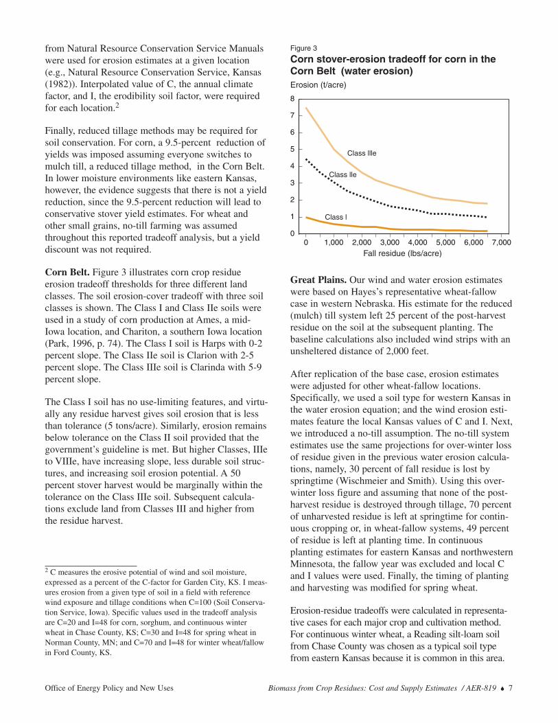
Corn Belt. Figure 3 illustrates corn crop residueerosion tradeoff thresholds for three different landclasses. The soil erosion-cover tradeoff with three soilclasses is shown. The Class I and Class IIe soils wereused in a study of corn production at Ames, a mid-Iowa location, and Chariton, a southern Iowa location(Park, 1996, p. 74). The Class I soil is Harps with 0-2percent slope. The Class IIe soil is Clarion with 2-5percent slope. The Class IIIe soil is Clarinda with 5-9percent slope.

The Class I soil has no use-limiting features, and virtu-ally any residue harvest gives soil erosion that is lessthan tolerance (5 tons/acre). Similarly, erosion remainsbelow tolerance on the Class II soil provided that thegovernment’s guideline is met. But higher Classes, IIIeto VIIIe, have increasing slope, less durable soil struc-tures, and increasing soil erosion potential. A 50percent stover harvest would be marginally within thetolerance on the Class IIIe soil. Subsequent calcula-tions exclude land from Classes III and higher fromthe residue harvest.

Great Plains. Our wind and water erosion estimateswere based on Hayes’s representative wheat-fallowcase in western Nebraska. His estimate for the reduced(mulch) till system left 25 percent of the post-harvestresidue on the soil at the subsequent planting. Thebaseline calculations also included wind strips with anunsheltered distance of 2,000 feet.

After replication of the base case, erosion estimateswere adjusted for other wheat-fallow locations.Specifically, we used a soil type for western Kansas inthe water erosion equation; and the wind erosion esti-mates feature the local Kansas values of C and I. Next,we introduced a no-till assumption. The no-till systemestimates use the same projections for over-winter lossof residue given in the previous water erosion calcula-tions, namely, 30 percent of fall residue is lost byspringtime (Wischmeier and Smith). Using this over-winter loss figure and assuming that none of the post-harvest residue is destroyed through tillage, 70 percentof unharvested residue is left at springtime for contin-uous cropping or, in wheat-fallow systems, 49 percentof residue is left at planting time. In continuousplanting estimates for eastern Kansas and northwesternMinnesota, the fallow year was excluded and local Cand I values were used. Finally, the timing of plantingand harvesting was modified for spring wheat.

Erosion-residue tradeoffs were calculated in representa-tive cases for each major crop and cultivation method.For continuous winter wheat, a Reading silt-loam soilfrom Chase County was chosen as a typical soil typefrom eastern Kansas because it is common in this area.

2 C measures the erosive potential of wind and soil moisture,expressed as a percent of the C-factor for Garden City, KS. I meas-ures erosion from a given type of soil in a field with referencewind exposure and tillage conditions when C=100 (Soil Conserva-tion Service, Iowa). Specific values used in the tradeoff analysisare C=20 and I=48 for corn, sorghum, and continuous winterwheat in Chase County, KS; C=30 and I=48 for spring wheat inNorman County, MN; and C=70 and I=48 for winter wheat/fallowin Ford County, KS.

Figure 3

Corn stover-erosion tradeoff for corn in theCorn Belt (water erosion)Erosion (t/acre)

0 1,000 2,000 3,000 4,000 5,000 6,000 7,0000

1

2

3

4

5

6

7

8

Fall residue (lbs/acre)

Class llle

Class lle

Class l


Reading Class I soil has a 0-2 percent slope and theClass II soil has a 2-4 percent slope. For the winterwheat-fallow area, Harney silt-loam soil from FordCounty in western Kansas was used. The most commonHarney soil has a 0-2 percent slope. Corn and sorghumerosion estimates are also based on Reading and Harneysoils. For spring wheat, a Kittson soil and a Barres soilfrom Norman County in northwest Minnesota approxi-mate typical situations. Class I Kittson soil has a 0-2percent slope and Class II Barres has a 3-5 percent slope.

The inclusion criterion is that the sum of wind andwater erosion rates are within tolerance after a residueharvest. The charts in fig. 4 depict the harvest margin.Generally, a substantial residue harvest is consistentwith erosion rates moderately below tolerance. Forcontinuous winter wheat on Class II land (fig. 4a), thetotal erosion rate is about 3 tons/acre with a 715 lb/acreresidue cover, which is below the 5 ton/acre tolerance.For spring wheat on Class IIIe land (fig. 4b), the totalerosion rate is about 6 ton/acre with a 750 lb residuecover, which is near the 5 ton/acre tolerance. For winterwheat/ fallow on Class II land, the erosion rate drops tothe 5 ton/acre tolerance when a fall residue of about1,500 lb/acre is left after harvest (fig. 4c).

Thus, harvest of wheat residues up to the 715 lb/acregovernment recommendation (required to comply withsoil-cover regulations) is suitable for continuouswinter wheat in land Classes I or II. Similarly,removing residue for spring wheat and leaving onlythe government’s minimum cover appears sensible forland in Classes I, II, or III. A partial harvest, whichwould leave at least 1,500 lb/acre of residue cover, isindicated for the wheat-fallow tradeoff on Class II landin western Kansas. In the last case, the 30-percent lossis a critical assumption for the marginal results.Slightly lower residue losses move the Class II wheat-fallow case into a higher harvest margin.

Erosion estimates for sorghum and corn on the Class Iland in eastern Kansas are also presented in figures 4dand 4e. First, sorghum harvest is at the 5-ton/acretolerance with the 1,430-lb/acre cover. Second, thecorn estimate falls below tolerance, unless 2,500lb/acre of residue remains. Wind erosion is the limitingfactor in both of these cases. Thus, residue harvest onClass I land planted to corn or sorghum is suitable;however, for corn, the unharvested residue shouldexceed the minimum government allowance.

Delta. Water erosion is not a problem on the flat land of the Mississippi Delta, thus the standard NaturalResource Conservation Service recommendation for soilcover is not relevant to the flat soils in the MississippiRiver Basin. But fermenting rice straw provides foodfor migrating waterfowl (Young). Residue harvest, up tothe point when the food needs of migrating waterfowlare met, does not present a conflict. Ideally, estimationof waterfowl demands would depend on the duck popu-lation that travels through the Delta, how long they stayin the Delta region, and how much they eat in a day.Until these estimates become available, a partial residueharvest may be best.

Southeast. Sugarcane bagasse is part of the raw sugar-cane stalk; so harvest and transport of bagasse to therefinery already occurs as part of the harvesting process.Thus, using bagasse has no change on soil conditions asit is already being removed.

A Harvest Cost Function

In developing general cost function, we noticed thatsome costs are constant on a per-acre basis while othersare constant on a per-unit output basis. We used the samecost parameters for all counties and crops; however, theresidue yield and fertilizer replacement rate vary acrosscrops and counties.

Direct harvest costs are approximated by machineryreplacement and operating costs for harvesting hay inlarge round bales. The cost estimates allow for threeoperations: chopping, baling, and on-farm transportation.Field operation costs for chopping and baling are basedon estimates from the Society for Agricultural Engineers.Capital replacement cost estimates were provided byCross and Perry. Lazarus adapted these cost studies for1997 conditions. First, estimates for fixed costs are usedas reported. Similarly, the reported operating expenses,$1.47/acre for chopping and $4.63/acre for baling, arealso used. Reported labor requirements and the local farmwage are important components of the operating expenseestimates.3 The chop and bale costs are all fixed on a per-acre basis. The cost of moving the bales to a convenient

3 The labor requirements for the chopper and the baler are thesame. The calculation is:

1 mach hr x 1.1 worker hr x $7.76 = $ 1.83 4.65 acre 1.0 mach hr worker hr acre

Local variation in the farm wage was investigated but had littleeffect on harvest cost.


site for on-farm storage is taken from Duffy and Judd.The farm haul costs are fixed on a per-ton basis.

Indirect fertilizer costs account for the additional needswhen residues are harvested. Unused residues providesome phosphorous, potassium, and nitrogen when leftfor the subsequent crop. Nutrient content tables for theresidues of major crops (corn, sorghum, barley, oats,wheat, rice, bagasse) are available (Bath et al.). Thesetables include direct estimates of phosphorous (P) andpotassium (K). The nitrogen (N) estimate was devel-oped using a protein conversion factor from Russell.The costs of replacing fertilizer associated with residueharvest in 1997 are: $6.466 per ton for corn, $4.988 per

Figure 4

Great Plains crop residue erosion tradeoffs

4a—Eastern Kansas, Class ll, continuous winter wheatErosion (t/acre)


Etotal

Ewater

Ewind

0 500 1,000 1,500 2,000 2,500 3,000 3,500 4,0000

1

2

3

4

5

6

7

8

4d—Corn, Class l

Erosion (t/acre)


Etotal

Ewater

Ewind

442945

1,5872,346

3,2074,152

5,1776,259

7,4088,607

9,856

11,151

12,489

13,856

0

1

2

3

4

5

6

7

8

9

4b—Minnesota, Class llle, spring wheat

Erosion (t/acre)


Etotal

Ewater

Ewind

0 500 1,000 1,500 2,000 2,500 3,000 3,500 4,0000

2

4

6

8

10

12

14

16

18

4e—Sorghum, Class l

Erosion (t/acre)


Etotal

Ewater

Ewind

264570

9651,438

1,9792,574

3,2233,918

4,6545,428

6,2367,075

7,9458,840

0

1

2

3

4

5

6

7

8

9

4c—Kansas, Class lle, winter wheat-fallow

Erosion (t/acre)


Etotal

Ewater

Ewind

0 500 1,000 1,500 2,000 2,500 3,000 3,500 4,0000

5

10

15

20

25

30

35


ton for wheat, $5.916 per ton for sorghum, $7.491 perton for barley, $7.858 per ton for oats, $5.42 per ton forrice, and $3.95/per ton for sugarcane bagasse. Thesecosts vary because fertilizer and nutrient content vary.For crops of the Midwest, fertilizer replacement costsvary about 50 percent from wheat to oats.

A harvest cost function that holds for all crops andcounties in 1997 depends on the government conserva-tion allowance (R, in dwt/acre) and the gross stoveryield (Yg, in dwt/acre). The cost estimate belowdefines the determinants of stover costs (C, in $/dwt):

The first term shows all of the costs that are constant ona per-acre basis. Specifically, chop and bale costs arerelated to trips across the field. So chop and bale costson an output basis are inversely related to yield. Thesecond term contains all costs that are constant on a per-unit output (ton) basis. On-farm hauling costs ($1.18 perton) are constant on an output basis because activityvaries with the number of bales hauled. Fertilizerreplacement costs, given above, are also proportional toresidue yield. The second term is the sum of on-farmhauling and fertilizer costs. It varies from commodity tocommodity depending on the fertilizer value.

The gross yield estimates are calculated from countyaverage yields using the biological relationships. Forinstance, corn stover constitutes 55 percent of the drymatter of the corn plant (Aldrich et al.; Park)4.Residue-yield relationships for other Midwestern cropsare taken from Plaster; Khush gives estimates of therice, straw, grain-yield relationship; and Paturauprovides bagasse yields from sugarcane.

Cost Estimates

A summary of cost estimates is given in table 2.Harvest and transport costs for typical situations aregiven. These examples indicate the range of plausibleharvest costs and processing plant sizes.

Harvest costs for dominant crops in important produc-tion regions indicate the situation under good circum-stances. Estimates are based on the harvest cost

function. Cost differences across commodities and loca-tions stem from variation in yield, conservationallowances, and opportunity values. Corn clearly has thelowest cost, especially with the exceptionally highyields from irrigated corn in the Great Plains. Harvestcosts for some other major crops of the winter wheatarea, wheat and sorghum in Riley County, KS, areslightly higher, at about $16 per ton. In the spring wheatarea, residue costs for wheat, barley, and oats are higheryet, in the $17-19 per ton range. Rice costs include asubstantial opportunity value reported by Wailes.Consequently, overall harvesting, fertilizer replacement,and opportunity costs total about $20 per ton because alarge opportunity value for forgone hunting rights isincluded. Finally, the winter wheat-fallow combinationin Ford County, KS, is the highest cost form of residuedue to the synergistic effects of low yields and highconservation requirements. Details of the harvest costcalculations are given in appendix tables A1-A10.

Transport costs depend on the density of crop residues,the size of the processing plant, and a given haulingrate. Transport cost estimates can be specified usingplausible biomass plant capacities and typical densityconditions. For instance, for Story County, IA, densityis dy = 889.4 ton/mi2, enough to support a very largeethanol plant (Q = 2.9 million tons of residue) withmoderate transport costs of about $2.15 per ton. Butthe transport-cost differential between the large plantand the small plant increases rapidly when the supplydensity falls below dy=500 per ton/mi2. Moderatetransport costs are given in table 2 with a mid-sizedethanol plant in the spring wheat and rice areas, whereresidue density is mid-range. The lowest density intable 2, Riley County, KS, gives moderate transportcosts with an electric plant much smaller than the mid-sized ethanol plant. Ultimately, a full analysis ofeconomies of scale should be conducted. Nonetheless,these estimates show that crop residues would beavailable to processing plants in the range of $14-$30per ton for all major field crops and regions.

Sugarcane bagasse is an exception to the harvest costfunction. The harvest, transport, and fertilizer replace-ment costs for bagasse are associated with the primarysugar crop. Hence, the costs of harvesting and deliv-ering bagasse to the plant are essentially zero.

Feed Value Estimates

Multiple steps in the residue supply curve can occurbecause livestock feed value varies with the type of

~

4 Lipinski et al. use a slightly lower estimate for the stover compo-nent of the corn plant’s dry matter (p. 106). But Park’s recentexperiments in Iowa confirm Aldrich’s calculations.

FRY

C ig

+−

= 93.15


residue. In turn, the livestock feed value varies with thetotal nutrient content and protein content of the residue.The hay price discount formulas of Stohhbehn andAyres were used for residue feed value estimates. Also,a recent feed composition table gives the componentspresent in various types of residues (Bath et al.). Theestimates in table 3 vary widely, ranging from about $6per ton for sugarcane bagasse to $43 per ton forsorghum stover. The variation in feed values reflectsdifferences between residues in protein content.

Supply Curves

Supply curves are constructed assuming that producersin a county will enter the market at the breakeven pointwhere the price of residue equals the harvest cost.

Variation in yields around a region will be an importantreason for supply variation. The supply curves in figure5 were developed using a two-step procedure. First, thecounty data were sorted on the computer by cost,

Table 2—A summary of residue harvest and transport costs

Commodity Location Harvest Residue Transport Totalcost density cost cost

$/ton t/mi 2 $/t $/ton

Type of plantCorn Story County, IA 12.73 889.4 2.15 14.88

Large ethanol

Winter wheat, continuous Riley County, KS 15.66 28.47 17.52Sorghum 16.6 12.36 18.46

sum 40.83 1.86

Electric

Winter wheat, continuous Ford County, KS 20.97 26.38 24.36Winter wheat, fallow 29.78 45.28 33.17Sorghum 16.73 0 20.12Corn 12.43 0 15.82

sum 71.66 3.39

Ethanol

Spring wheat, continuous Norman County, MN 19.42 246.3 21.00Barley 17.34 77.8 18.92Oats 18.56 3.96 20.14

sum 328.06 1.58

Ethanol

Rice Arkansas County, AR 20.32 283.24 1.70 21.90

Ethanol

Transport cost ($/ton/mile) 0.1

Plant input requirements (tons)100,000 electric plant581,000 ethanol plant

2,900,000 large ethanol plant

Table 3—Cattle feed value by type of residue

Type Value

Dollars/ton

Corn stover 41.90Sorghum stover 42.51Wheat straw 21.21Barley straw 32.09Oat straw 34.25Sugarcane bagasse 6.31Rice straw 25.10


tracking the associated net residue supply volume foreach county. Then the quantities were cumulated, givingthe total amount available in local residue markets at agiven price.

Figure 5a gives the Corn Belt farm supply curve forcorn stover. It suggests a highly elastic response at thefarm level. If prices vary by little more than $2 per ton,ranging from about $12 to $14.50 per ton, the supplywould go from zero to about 90 percent of the availablestover supply (180 billion pounds) in the Midwest.Large plants have greater input cost variation thansmaller plants reflecting variations in both yield and thegeographical density of corn supplies. In a $6 per tonrange from about $16.50 per ton to $22 per ton, thesupply ranges from zero to about 90 percent of avail-able stover. Finally, a 10-percent increase in the stovervolume (not shown) is available at a much higher priceof $42 per ton, the price of bidding these residues awayfrom use as livestock feed. The diagram includes trans-port costs for a small ethanol plant and a large ethanolplant, respectively. The difference between the costcurves for a large plant and a small plant starts at about$2.50 per ton. It widens rapidly above 175 millionpounds due to locations with exhausted high-densitycorn supplies.

The analysis for residue supply in the Great Plains ismore complex due to the various costs of residuesources. Prices in the residue supply curve (fig. 5b) arethe average input costs for a plant that follows theleast-cost rule for use of inputs. Corresponding quanti-ties come from the efficient market areas. Other

supplies are available at the higher cost after efficientmarket areas are depleted.

The Great Plains supply curve (fig. 5b) includes thetransport charges associated with a middle-sized ethanolplant. Crop residues would become available at about$14 per ton; at about $35 per ton, approximately 90percent of the residue supplies would become availableto the market. The increasing input costs reflectdeclining residue yields, increasing conservationrequirements, use of wheat feed residues, and decliningdensity of available residues.

The West Coast supply curve (fig. 5c) includes thetransport charges for an electric-biomass plant. Theinitial concave shape indicates that there is a pocketwhere concentrated low-cost residue is available.Otherwise, the wide range of supply prices occurs forall the same reasons given for the Great Plains. Therightward shift at $42 per ton reflects the diversion ofresidues from animal feed to industrial supply.

The Delta supply curve (fig. 5d) is flat; most of the strawwould become available within a range of about $20-25per ton. The supply curve is flat because the yield anddensity conditions are uniform in the rice area.

In the Southeast, sugarcane bagasse is burned for energyin sugar refineries. The bagasse in cane provides slightlymore energy than the modern plant requires: 100 tons of sugarcane produces 25 tons of bagasse (49 percentmoisture mill run) and 9 tons are not needed for sugarprocessing (Paturau). Some modern facilities also install

Figure 5a

Corn Belt crop residue supply

Price ($/ton)

Quantity (mil. lbs)

Large ethanol plant cost Small ethanol

plant cost

Farm cost

0

5

10

15

20

25

30

35

0 50,000 100,000 150,000 200,000 250,000

Figure 5b

Great Plains crop residue supply

Price ($/ton)

Quantity (mil. lbs)

Ethanol plant cost

0

10

20

30

40

50

60

0 20,000 40,000 60,000 80,000


generating equipment and sell electricity by burning thesurplus. Other manufacturers must pay more than theopportunity value of bagasse in sugar refining before itwill be supplied to others.

The opportunity value of heat from natural gas indi-cates the market supply price. The breakeven price forburning bagasse or natural gas with the same profit is

where P is price, Q is quantity, n is natural gas, and b isbagasse. For the 1997 baseline, the breakeven bagasse

price is $34.65 per ton. Supplies will be availableoutside the refinery if the bid exceeds this breakevenprice. The breakeven price is estimated from:

Overall, the bagasse supply price is on the high sidefor crop residues. Its price compares more closely tolivestock feed than to other biomass crops.

Biomass Supply and Capacity

Supply and utilization tables are useful for evaluatingthe supply potential of crop residues. Table 4 summa-rizes the regional supply situation. Net productionincludes conservation adjustments to yield anderosion-based restrictions required for the harvestedarea. Feed use indicates livestock demand minus haysupplies. Industry supply refers to unused residues thatwould be available to a biomass processing industry ata price near the harvest cost.5

The total biomass supply ranges from 297 to 313billion pounds, depending on the price level. Corn Beltresidues account for two-thirds of available residues.But the Great Plains account for nearly a quarter ofavailable supplies. The other regions provide pocketsof low-cost crop residues.

If the trends of the last two decades continue, growthshould occur in the crop residue resource due toincreased crop yields and declining livestock demandfor forage. First, a repeat of crop productivity growthof 56 percent over the last two decades would accountfor another 170 billion pounds of crop residues. Also,the 10-percent decline in cattle populations of the lasttwo decades could account for another 75 billionpounds of available biomass in another two decades.Hence, the biomass residue supply could grow toabout 500 billion pounds during the next two decades.

Existing residue supplies could also make a differencein U.S. energy markets. Tomorrow’s biomass ethanoltechnology could displace petroleum inputs (Gallagher

Figure 5c

West Coast crop residue supply

Price ($/ton)

Quantity (mil. lbs)

Electric plant cost

0

10

20

30

40

50

60

0 1,000 2,000 3,000 4,000 5,000 6,000 7,000

Figure 5d

Delta crop residue supply

Price ($/ton)

Quantity (mil. lbs)

Ethanol plant cost

Farm cost

0

5

10

15

20

25

30

35

40

0 2,000 4,000 6,000 8,000 10,000

, Q / QP P bnnb =

bm.ton59.2

n m.ton1Q / Q

,1m.ton

nft4310.44:conversion ,

ft10

02.2$P

bn

33

33b

=

=

5 State-level estimates of the supply and utilization tables are givenin appendix B.


and Johnson). The petroleum displacement with allcrop residue supplies is:

313 bil lb res x 1 gal ethanol x 1 ton res x.0083 ton res 2,000 lb res

1 bbl x 0.84 bbl oil = 0.377 bil bbl oil.42 gal bbl

Hence, ethanol processing from residues coulddisplace 12.5 percent of U.S. petroleum imports in the1997 baseline year. Alternatively, electricity displace-ment could occur with today’s biomass conversiontechnology. Using the crop residue/electricity yieldsfrom Larsen, the electricity equivalent of the residuecapacity is:

313 bil lb res x 1 kWh x 1.1 mt ton res x .000998 mt res ton res

1 ton res = 172.4 bil. kWh2,000 lb res

Hence, biomass electricity from residues could physi-cally account for 5 percent of U.S. electricityconsumption. However, energy displacements referonly to possibilities at present. The biomass ethanoltechnology is still under development. Biomass elec-tricity processing is in operation in Denmark but maysucceed in the United States only with high rates ofutilization and local markets for byproduct heat.

Summary and Conclusions

This study has examined biomass supply from cropresidues, taking into account cost and environmentalfactors. First, the analysis suggests that reduced tillageand partial residue harvest may maintain soil quality andincrease producer profits. Corn Belt, Great Plains, andWest Coast participation is possible with judicious selec-tion of crops and areas. Second, residues are probablythe lowest cost form of biomass supply. Throughout theCorn Belt, residue costs have a narrow price range, from$16 to $18 per ton, even after making allowances fordelivery to a large plant. The range of costs is wider inthe Great Plains due to diverse growing conditions,conservation requirements, and forage demands. Theeastern section of the spring wheat area has extensiveresidue supplies at moderate costs. Also, the easternsection of the winter Wheat Belt has a cost advantagewhen feed grain residues, wheat straw, and residuesdiverted from feed are combined. The remaining regions,the West Coast, the Delta, and the Southeast, havepockets with residue supplies.

Crop residues are a low-cost resource with the potentialto displace 12.5 percent of petroleum imports or 5percent of electricity consumption in today’s markets.The residue resource also has growth potential fromcrop productivity and declining livestock demands for forage. Taken with other potential sources, likeConservation Reserve Program (CRP) and hay land,biomass supply from crop agriculture could provide asubstantial share of U.S. energy consumption. The agri-culture sector can benefit from an increased presence inenergy and industrial product markets, given steadyproductivity growth and stagnant traditional markets.

Table 4—Biomass from crop residues: Supply and capacity for 1997 baseline

Net residue Feed IndustryRegion production use supply

Mil lbs.

Corn Belt 207,199 23,786 197,844

Great Plains 81,040 9,994 71,042

West Coast 7,377 2,573 4,805

Delta (Rice) 10,435 1,168 9,246

Southeast (Sugar bagasse) 7,114 0 7,114

Total 313,165 37,521 290,051


References

Aldrich, S.R. , W.O. Scott, and E.R. Leng, ModernCrop Production, A&L, 1978.

Committee on Beef Cattle Nutrition, Nutrient Require-ments of Beef Cattle, National Academy Press, 1996.

Committee on Biobased Industrial Products, BiobasedIndustrial Products: Priorities for Research andCommercialization, National Research CouncilReport, Washington, DC, August 1999.

Bath, D., J. Dunbar, J. King, S. Berry and S. Olbrich,“Byproducts and Unusual Feedstuffs,” Feedstuffs,70(1998): 32-38.

Cross, T. and G. Perry, “Depreciation Patterns forAgricultural Machinery,” American Journal of Agri-cultural Economics (Feb. 1995): 194-204.

Duffy, M., and D. Judd, Estimated Costs of Crop Pro-duction in Iowa 1994, FM1712, Ames, Iowa: IowaState University Extension, Ames, IA , January1994.

Gale, W. J., and C. A. Cambardella, “Carbon dynamicsof surface residue- and root-derived organic matterunder simulated no-till.” Soil Science Social Ameri-can Journal 64(1):(2000).

Gallagher, Paul, and Donald Johnson, “Some NewEthanol Technology: Cost Competition and Adop-tion Effects in the Petroleum Market. The EnergyJournal 20(2):89-120. 1999.

Hayes, William A., “Estimating Wind Erosion in theField,” Proceedings of the Soil Conservation Soci-ety of America (Aug 1975):138:143, San Antonio,Texas

Hawkins, R., et al., PLANETOR Users Manual, St.Paul: Center for Farm Financial Management, Uni-versity of Minnesota, 1995.

Hoag, D.L., and H.A. Holloway, “Farm ProductionDecisions under Cross and Conservation Compli-ance,” American Journal of Agricultural Economics,(1991):184-193.

Jurgens, M.H., Animal Feeding and Nutrition,Kendall/Hunt Co. Dubuque, 1993.

Klingebiel, A. A., and P.H. Montgomery, “Land-Capa-bility Classification,” Agriculture Handbook No.210, U.S. Department of Agriculture, Soil Conser-vation Service, 1961.

Khush, G., “Breaking the Yield Frontier in Rice,”Geojournal (1993):331-3.

Larsen, J.B., “Firing Straw for the Production of Elec-tricity with and without Producing District Heat-ing,” in R.P. Overend and E. Chornel, eds., Makinga Business From Biomass, Proceedings of a Confer-ence in Montreal, 1997, Pergamon Press.

Lazarus, W., Minnesota Farm Machinery EconomicCost Estimates for 1997, Minnesota Extension Service, St. Paul, 1997.

Lipinsky, E.S., T.A. McClure, J.L. Otis, D.A. Scant-land, and W.J. Sheppard, Systems Study of Fuelsfrom Sugarcane, Sweet Sorghum, Sugar Beets andCorn, Vol. IV “Corn Agriculture,” Columbus, OH:Battelle Columbus Laboratories Report No. BMI-1957a (Vol. 4), March 1977.

Park, Y., Costs of Producing Biomass Crops in Iowa,Ph.D. Dissertation, Ames: Iowa State University,1996.

Paturau, J.M., By-Products of the Cane SugarIndustry, Elsevier Co., Amsterdam, 1982.

Perry, G.M., B.A. McCarl, M.E. Rister, and J.W.Richardson, “Modeling Government Program Par-ticipation Decisions at the Farm Level,” AmericanJournal of Agricultural Economics(1989):1011-1020.

Plaster, E.J., Soil Science & Management, Delmar Co.,Albany, 1992.

Reicosky, D.C., S.D. Evans, C.A. Cambardella, R. R.Allmaras, A.R. Wilts, and D.R. Huggins, “Continu-ous Corn with Moldboard Tillage: Silage and Fertil-ity Effects on Soil Carbon,” Soil Science SocialAmerican Journal, 2000.

Renard, K.G., G.R. Forster, D.K. McCool, G.A.Wessies, and D.C. Yoder. RUSLE User’s Guide.Ankeny, IA: Soil and Water Conservation Society,1993.


Russell, J.R., M. Brasche, and A.M. Cowen, “Effectsof Grazing Allowance and System on the Use ofCorn Crop Residues by Gestating Beef Cows,”Journal of American Science, 71(1993):1256-5.

Shimojo, T., “Economic Analysis of ShippingFreights.” Research Institute for Economics andBusiness Administration, Kobe University, 1979.

Skidmore, E.L., and N.P. Woodruff, Wind ErosionForces in the United States and Their Use in Pre-dicting Soil Loss, Agriculture Handbook No. 346,U.S. Department of Agriculture, April 1968.

Spelman, C.A., “Nonfood Uses of Agricultural RawMaterials: Economics,” Biotechnology and Politics,CAB International, Wallingford, UK, 1994.

Stohbehn, D., and G.E. Ayres, Pricing Machine-har-vested Corn Residue, Ames, IA: Cooperative Exten-sion Service, Iowa State University, December1976.

U.S. Department of Agriculture, Soil Conservation Service, KS, T.G. Notice KS-93, Dodge City, KS,June 1982.

U.S. Department of Agriculture, Soil ConservationService, IA, The Wind Erosion Equation, TechnicalGuide, Section I-C-2, March 1987.

U.S. Department of Agriculture, Soil ConservationService, Conservation Catalog for the 1990’s, DesMoines, IA: October 1991.

U.S. Department of Agriculture Soil Survey Staff-Nat-ural Resources Conservation Service, National SoilSurvey Handbook, Title 430-VI, November 1996.

Wailes, E., “Farmer Survey of On-Farm ReservoirInvestment Study,” Department of Agricultural Eco-nomics, University of Arkansas, Fayetteville, AR,1999.

Wischmeier, W.H., and Smith, D. D., Predicting Rain-fall Erosion Losses—A Guide to Conservation Plan-ning, Agriculture Handbook No. 537, U.S. Depart-ment of Agriculture, 1978.

Young, M. “Duck Gumbo,” Ducks Unlimited February(1999):54-58.


Appendix tables A—Costs

Appendix table A-1—Story County, Iowa, corn stover harvest costs

Corn yield (bu/acre) 147Gross stover yield (dw lb/acre) 7694.153Conservation (dw lb/acre) 1430 (dwt/acre) 0.715Net stover yield (dw lb/acre) 6264.153 (dwt/acre) 3.132077

Direct harvest costs

Operation Fixed costs Variable costs Total costsReported Per ton s Reported Per ton s

Chop 2.98 ($/acre) 0.951445 ($/ton) 3.31 ($/acre) 1.056807 ($/ton s) ($/ac)Bale 3.15 ($/acre) 1.005723 ($/ton) 6.49 ($/acre) 2.072108 15.93Haul 0.51 ($/ton) 0.67 ($/ton)

2.467168 ($/ton) 3.798915 6.266083 5.086083

Fertilizer replacement costs

Fertilizer application rates Fertilizer price Fertilizergross Dilute Strength Pure expense

(t f/ dwt s) ($/ton f) ($/ton f) ($/ton s)P2o5 $0.00 257 0.45 571.1111 0.916062K2o $0.01 152 0.60 253.3333 3.097507 ($/ton)NH3 0.008093 303 1.00 303 2.452179 6.465748 7.645748

Total direct & fertilizer($/ton s) 12.73183 12.73183Note: dw = dry weight. $/ton f = dollars per ton of fertilizer. $/ton s = dollars per ton of stover or straw. tf = tons fertilizer.

Appendix table A-2—Riley County, Kansas, continuous winter wheat, straw harvest costs

Wheat yield (bu/acre) 40.7Gross straw yield (dw lb/acre) 4070Conservation (dw lb/acre) 715 (dwt/acre) 0.3575Net straw yield (dw lb/acre) 3355 (dwt/acre) 1.6775




4.16424 ($/ton) 6.512027 10.67627 9.496274






Appendix table A-3—Riley County, Kansas, sorghum stover harvest costs

Sorghum yield (bu/acre) 80.9Gross stover yield (dw lb/acre) 4854Conservation (dw lb/acre) 1500 (dwt/acre) 0.75Net stover yield (dw lb/acre) 3354 (dwt/acre) 1.677




4.165337 ($/ton) 6.513769 10.67911 9.499106





Appendix table A-4—Ford County, Kansas, wheat/fallow, straw harvest costs

Wheat yield (bu/acre) 28.491Gross straw yield (dw lb/acre) 2849.1Conservation (dw lb/acre) 1500 (dwt/acre) 0.75Net straw yield (dw lb/acre) 1349.1 (dwt/acre) 0.67455




9.59754 ($/ton) 15.1982 24.79574 23.61574






Appendix table A-5—Ford County, Kansas, sorghum stover harvest costs

Sorghum yield (bu/acre) 80.2Gross stover yield (dw lb/acre) 4812Conservation (dw lb/acre) 1500 (dwt/acre) 0.75Net stover yield (dw lb/acre) 3312 (dwt/acre) 1.656




4.211691 ($/ton) 6.587874 10.79957 9.619565





Appendix table A-6—Ford County, Kansas corn stover harvest costs

Corn yield (bu/acre) 173.1Gross stover yield (dw lb/acre) 9060.258Conservation (dw lb/acre) 2400 (dwt/acre) 1.2Net stover yield (dw lb/acre) 6660.258 (dwt/acre) 3.330129




2.35077 ($/ton) 3.612829 5.963599 4.783599



(t f/ dwt s) ($/ton f) ($/ton f) ($/ton s)O2o5 $0.00 257 0.45 571.1111 0.916062K2o $0.01 152 0.60 253.3333 3.097507 ($/ton)NH3 0.008093 303 1.00 303 2.452179 6.465748 7.645748



Appendix table A-7—Norman County, Minnesota, spring wheat, straw harvest costs

Wheat yield (bu/acre) 31.193Gross straw yield (dw lb/acre) 3119.3Conservation (dw lb/acre) 715 (dwt/acre) 0.3575Net straw yield (dw lb/acre) 2404.3 (dwt/acre) 1.20215




5.609197 ($/ton) 8.822061 14.43126 13.25126





Appendix table A-8—Norman County, Minnesota, barley straw harvest costs

Barley yield (bu/acre) 54.9Gross straw yield (dw lb/acre) 4392Conservation (dw lb/acre) 715 (dwt/acre) 0.3575Net straw yield (dw lb/acre) 3677 (dwt/acre) 1.8385




3.84424 ($/ton) 6.000432 9.844672 8.664672






Appendix table A-9—Norman County, Minnesota, oat straw harvest costs

Oat yield (bu/acre) 67.7Gross straw yield (dw lb/acre) 4062Conservation (dw lb/acre) 715 (dwt/acre) 0.3575Net straw yield (dw lb/acre) 3347 (dwt/acre) 1.6735




4.172982 ($/ton) 6.52599 10.69897 9.518972





Appendix table A-10—Arkansas County, Arkansas, rice straw harvest costs

0.845Rice yield (lb/acre) 6200Gross straw yield (dw lb/acre) 5239Conservation (dw lb/acre) 0 (dwt/acre) 0Net straw yield (dw lb/acre) 5239 (dwt/acre) 2.6195



Chop 2.98 ($/acre) 1.137622 ($/ton) 3.31 ($/acre) 1.2636 ($/ton s) ($/ac)Bale 3.15 ($/acre) 1.20252 ($/ton) 6.49 ($/acre) 2.477572 35.93Hunting lease 20 ($/acre) 7.635045Haul 0.51 ($/ton) 0.67 ($/ton)

10.48519 ($/ton) 4.411172 14.89636 13.71636



(t f/ dwt s) ($/ton f) ($/ton f) ($/ton s)P2o5 0.00128 257 0.45 571.1111 0.732736P2o 0.01113 152 0.60 253.3333 2.8196 ($/ton)NH3 0.006713 303 1.00 303 1.870419 5.422755 6.602755



Appendix tables B—QuantityA

pp

end

ix t

able

B-1

—C

orn

Bel

t,co

rn s

tove

r su

pp

ly a

nd

use

Sta

teIL

INIA

KS

KY

MN

MO

NE

OH

SD

WI

Tota

l

Cor

n yi

eld

( bu/

acre

)13

912

913

713

411

811

712

612

590

104

Cor

n st

over

yie

ld (

lb/a

cre)

5,61

35,

063

5,48

95,

323

4,54

94,

505

4,95

64,

883

3,12

43,

826

Cor

n ar

ea:

Ero

dibl

e fr

actio

n (0

/1)

0.16

70.

1705

0.32

560.

2449

0.41

740.

1534

0.43

910.

4674

0.47

390.

2926

0.27

37H

arve

sted

for

stov

er (

mil.

acre

)9.

3296

5.05

995

8.90

208

1.39

6935

0.82

7292

6.09

552

1.40

225

4.42

058

1.99

918

2.68

812

2.83

179

44.9

533

Cor

n st

over

pr

oduc

tion

( mil.

lb)

52,3

70.5

2,52

49.8

44,7

41.2

9,10

5.7

27,4

13.1

7,40

3.2

22,9

30.8

13,4

95.7

8,29

5.3

10,6

67.6

620

7,19

8.5

Net

cor

n st

over

fo

rage

dem

and

( mil.

lb)

00

2,71

1.0

4,73

6.3

05,

047.

27,

563.

00

1,12

3.9

2,60

6.8

23,7

86

Net

cor

n st

over

sup

ply

for

indu

stria

l pr

oces

sing

(m

il.lb

)52

,370

.525

,249

.842

,030

.24,

369.

427

,413

.12,

355.

915

,367

.713

,495

.77,

171.

38,

060.

819

7,88

4.4


Appendix table B-2—Great Plains: Residue supply for industrial processing

State CO KS MN MT NE ND OK SD Total

Million lbs

Total residue production 2,130 24,518 5,471 7,622 3,447 30,464 2,825 4,563 81,040

Net residue forage demand 907 5,085 0 725 1,348 121 1,651 157 9,994

Net residue supply forindustrial processing 1,223 19,433 5,470 6,896 2,098 30,343 1,174 4,405 71,042

Appendix table B-3—Production and use of Great Plains residues, by crop and State, 1997 baseline

State Crop Residue yield Erodible Non-erodible Production Livestock use Industrial use

Lbs/acre Fraction Mil. acres Mil. lbs Mil. lbs Mil. lbs

CO Barley 2,913 0.43 .003 7.9 1.2 6.7Corn 4,186 0.72 .248 1,038.1 506.6 531.6Oats 0 1.00 0 0 0 0S Wheat 0 1.00 0 0 0 0Sorghum 1,054 0.70 .043 45.5 18.4 27.1W Wheat (Cont) 2,235 0.60 .062 139.7 87.8 51.8W Wheat (Fallow) 1,553 0.74 .579 899.4 293.3 606.1

KS Barley 0 1.00 0 0 0 0Corn 6,341 0.58 1.025 6,500.1 2,402.7 4,097.4Oats 0 1.00 0 0 0 0S Wheat 0 1.00 0 0 0 0Sorghum 2,923 0.64 1.129 3,299.4 1,592.7 1,706.7W Wheat (Cont) 2,965 0.38 3.537 10,487.5 690.1 9,797.3W Wheat (Fallow) 1,996 0.57 2.120 4,231.5 399.7 3,831.8

MN Barley 4,076 0.39 .239 975.2 0 975.2Corn 2,691 0.63 .234 629.1 0 629.1Oats 2,870 0.39 .051 146.8 0 146.8S Wheat 2,740 0.37 1.354 3,708.9 0 3,709.0Sorghum 0 1.00 0 0 0 0W Wheat (Cont) 2,871 0.91 .004 10.5 0 10.5W Wheat (Fallow) 0 1.00 0 0 0 0

MT Barley 3,532 0.41 .430 1,517.8 534.5 983.3Corn 0 1.00 0 0 0 0Oats 2,557 0.38 .016 41.8 38.1 3.7S Wheat 2,670 0.37 2.206 5,890.6 152.5 5,738.1Sorghum 0 1.00 0 0 0 0W Wheat (Cont) 3,309 0.93 .007 24.1 0 24.1W Wheat (Fallow) 2,504 0.92 .058 147.3 0 147.3

NE Barley 0 1.00 0 0 0 0Corn 4,789 0.74 .408 1,953.9 843.3 1,110.6Oats 2,490 0.87 .002 4.9 0 4.9S Wheat 0 1.00 0 0 0 0Sorghum 3,566 0.66 .120 427.2 183.3 244.0W Wheat (Cont) 3,046 0.53 .110 335.4 100.6 234.9W Wheat (Fallow) 2,133 0.72 .340 725.2 221.3 503.9

ND Barley 3,804 0.14 1.941 7,386.0 47.5 7,338.5Corn 2,717 0.84 .123 333.9 14.2 319.7Oats 2,922 0.26 .306 894.8 47.9 847.0S Wheat 2,492 0.20 8.768 21,847.9 11.5 21,836.4Sorghum 0 1.00 0 0 0 0W Wheat (Cont) 2,245 0.97 0 1.6 0 1.6W Wheat (Fallow) 1,460 0.99 0 .4 0 .4

Continued--


Appendix table B-3—Production and use of Great Plains residues, by crop and State,1997 baseline--continued

State Crop Residue yield Erodible Non-erodible Production Livestock use Industrial use

Lbs/acre Fraction Mil acres Mil lbs Mil. lbs Mil. lbs

OK Barley 4,018 0.56 .000 1.7 0 1.6Corn 5,688 0.86 .018 107.5 107.5 0Oats 1,351 0.82 .005 6.6 5.6 1.1S Wheat 0 1.00 0 0 0 0Sorghum 1,795 0.78 .084 151.2 110.6 40.7W Wheat (Cont) 1,777 0.69 1.402 2,491.5 1,361.1 1,130.4W Wheat (Fallow) 1,303 0.78 .052 67.3 66.7 .6

SD Barley 3,268 0.45 .038 123.9 0 123.9Corn 1,753 0.75 .362 634.3 74.3 560.0Oats 3,007 0.29 .084 252.4 22.7 229.8S Wheat 2,579 0.39 1.012 2,610.1 59.1 2,551.0Sorghum 1,589 0.62 .004 6.4 1.9 4.5W Wheat (Cont) 3,093 0.40 .179 554.5 0 554.5W Wheat (Fallow) 2,274 0.56 .168 381.9 0 381.9

Totals 28.871 81,044.0 9,996.7 70,726.0

Appendix table B-4—West Coast: Residue supply for industrial processing

State CA OR WA Total

Million lbs

Total residue production 1,601.7 1,856.2 3,919.3 7,377.2

Net residue forage demand 1,467.8 641.2 463.7 2,572.7

Net residue supply forindustrial processing 133.9 1,215.0 3,455.7 4,804.6


Appendix table B-5—Production and use of West Coast residues, by crop and State, 1997 baseline

State Crop Residue yield Erodible Non-erodible Production Livestock Industrial

Lbs/acre Fraction Mil. acres Mil. lbs Mil. lbs Mil. lbs

CA Barley 4,686 0.43 .085 398.1 395.1 2.0Corn 2,161 0.08 .535 1,156.2 1,024.3 131.9Oats 5,910 0.91 .003 16.1 16.1 0S Wheat 0 1.00 0 0 0 0Sorghum 0 1.00 0 0 0 0W Wheat (Cont) 6,197 0.99 .005 30.0 30.0 0W Wheat (Fallow) 5,527 0.99 0 2.4 2.4 0

OR Barley 4,684 0.28 .084 391.3 161.1 230.2Corn 2,229 0.66 .016 35.6 33.2 2.4Oats 5,441 0.77 .007 39.3 24.3 15.0S Wheat 4,146 0.36 .077 319.7 73.9 245.8Sorghum 0 1.00 0 0 0 0W Wheat (Cont) 7,647 0.64 .109 835.0 296.8 538.1W Wheat (Fallow) 4,823 0.90 .049 235.4 51.9 183.6

WA Barley 4,320 0.67 .159 684.8 160.8 524.1Corn 6,12 0.69 .043 284.0 54.1 229.9Oats 3,892 0.30 .009 31.2 13.7 17.4S Wheat 4,143 0.48 .219 906.9 133.8 773.0Sorghum 0 1.00 0 0 0 0W Wheat (Cont) 5,924 0.76 .156 925.6 73.7 851.9W Wheat (Fallow) 4,557 0.84 .238 1,086.8 27.5 1,059.3

Totals: 1.794 7,378.4 2,806.1 4,804.6

Appendix table B-6—Delta: Rice straw supply and use

State AR LA MS MO TX Total

Rice yield (lb/acre) 5.700 4.837 5.774 5.385 5.465

Residue yield (lb/acre) 4.816 4.087 4.879 4.550 4.618

Harvested acres (mil. acre) 1.328 .493 .224 .112 .075 2.232

Residue production (mil. lbs) 6,472.3 1,985.8 1,102.2 505.1 369.9 10,435.3

Net residue forage demand (mil. lbs) 439 436 52 53 207 1,168.0

Industrial supply (mil. lbs) 6,033.3 1,549.8 1,050.2 452.1 162.0 9,246.3

Appendix table B-7—Southeast: Sugarcane bagasse supply and use*

State FL HA LA TX Total

Sugarcane yield (ton/acre) 35.36 81.88 26.64 30.77

Bagasse yield (tons/acre) 8.84 20.47 6.66 7.69

Harvested acres (mil. acre) .421 .032 .379 .027 0.859

Residue production (mil. ton) 3,721.9 655.0 2,527.1 210.0 7,114.0*mill run (49% moisture) basis


Glossary

Crop residue: Plant matter remaining after removingthe food or feed component.

Fallow/plant: The process of leaving land unseededduring one growing season, for purposes of wateraccumulation in semi-arid climates, and planting in asubsequent growing season.

Stover yield: The corn (or sorghum) residueproduced per acre of land planted to corn (orsorghum).

Harvest costs: For crop residues, the costs ofcollecting, chopping, baling, and moving residues toa central place on the farm. Fertilizer replacement isalso included.

Forage: Feed for livestock, often consisting ofcoarsely chopped corn residues, hay, straw and otherplanted material with high cellulose content.

Tillage: Cultivation of land.

No-till system: A crop production system that doesnot use a conventional plow to break-up the soil.Often, a drill is used to plant seeds.

Transport costs: Fuel, maintenance, and capitalcosts associated with using a truck or tractor to movebiomass from the farm to the processing plant.

Biomass: Plant matters grown to produce non-foodproducts, such as liquid fuel or electricity.

Biomass from Crop Residues: Cost and Supply Estimates.

Documents

Transcript of Biomass from Crop Residues: Cost and Supply Estimates.