Biological Acoustic Monitoring

John K. Horne

LO: Identify potential uses and limitations of acoustic technologies to

monitor biological quantities of interest

Applications & Objectives

Application Objective(s)

Ocean Observing Temporal trend ,

Environmental covariates

Hydropower Dams Fish passage routes,

abundance

Nuclear water cooling Clogging intakes

Marine Renewable Energy Device collisions, biological

impacts, abundance

Environmental Impact Pre/post disturbance

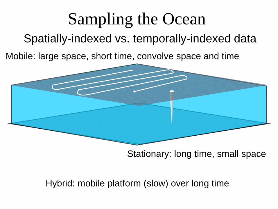
Sampling the OceanSpatially-indexed vs. temporally-indexed data

Mobile: large space, short time, convolve space and time

Stationary: long time, small space

Hybrid: mobile platform (slow) over long time

Steven Ackleson, US Consortium for Ocean Leadership

Ocean Observing Time Series

Expanding Scales in Ocean Observing

Ocean Observing, Observatories,

and Observing SystemsClassic:

Ocean observing: instruments used to observe water properties or water

contents

Observatory: central node(s) supplying power & communications to

instrument(s)

Evolving:

Observatory: stationary or mobile instruments using node infrastructure

Observing system: regional infrastructure or platform(s) supporting instrument

clusters

What’s Changed?

Infrastructure: from project based to program

- expansion from single site up to ocean basin, linking site infrastructures

- expansion and inclusion of mobile instruments, winched platforms

- expansion of infrastructure from surface or submerged node

Objectives: from explicit science and monitoring, to data acquisition for data

acquisition or modeling

Early Conceptual/Actual Observatories

LEO 15: Rutgers University, 1998 - 2001

Power

Communication

Platforms

Instruments

Network

Predictive

Coastal

Experiments

Early Conceptual/Actual ObservatoriesOcean Hub Monitoring, IMR, Norway, 2002-2008

MOOS: 38 kHz

MBARI: 1989 -

Progression of Ocean ObservingADCP: Krill DVM

Cochrane et al.

1994

Acoustic Lander: 38 kHz

MarEco 2004-2005

DEIMOS: 38 kHz

MARS-UW, 2009-2012

Progression of Ocean Observing

Memorial University, 2004-2005

Single Node Observatory Autonomous Deployment

for tidal energy baseline

University of Washington, 2011

Ocean Observing SystemsMulti-National or Global

Eurosites: 9 deep (>1000m)

GOOS: Global Ocean

Observing System

Ocean Observing SystemsNational or Bi-Lateral

IMOS: Integrated Marine

Observing System

RCOS: Regional Coastal

Observing Systems

OOI: Ocean Observatory Initiative 2015

Coastal Instrument Array

Global (3), Regional (1),

Coastal (2)

www.orionprogram.org/OOI/default.html

Acoustic Technologies Deployed

ADCP

Manufacturers: Aanderaa, Nortek, RDI, Seaguard

Frequency Range: 150 – 1200 kHz

Depths: 15 - ?

Echosounders

Manufacturers: ASL Environmental, BioSonics, Simrad

Frequency Range: 38 – 200 kHz

Depths: 20 - 1000 m

Deployment Platforms

Surface:

Stationary: buoys, moorings

Mobile: ships, waveglider, saildrone

Bottom:

dedicated cables; cabled nodes; autonomous

packages

Inbetween: stationary or winched platforms; gliders;

ROVs; AUVs

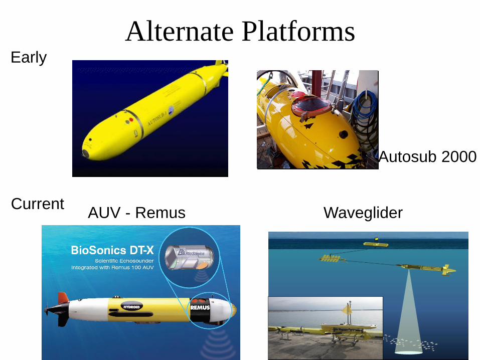
Alternate Platforms

Autosub 2000

Early

CurrentAUV - Remus Waveglider

Alternate Platform: Speed & Duration

Graphics: D. Hume

10

knt

Graphics: D. Hume

Depth

Alternate Platform: Maximum Depths

IMOS: Integrated Marine Observing System

Dedicated or Opportunistic Platforms

Rudy Kloser, Ryan Downing, Gordon Keith, Tim Ryan www.imos.org.au

Benoit et al. 2008, JGR.

250

200

150

100

50

0

Dep

th (

m)

December 18

250

200

150

100

50

0

Dep

th (

m)

February 10

250

200

150

100

50

0

Dep

th (

m)

March 31

250

200

150

100

50

0

Dep

th (

m)

June 1st

250

200

150

100

50

0

Dep

th (

m)

June 1st

-1.80000E+01

1.08333E+01

3.96667E+01

6.85000E+01

9.73333E+01

1.26167E+02

1.55000E+02

JOUR

0

10

20

30

40

50

60

70

BIO

MA

SS

EK

G

-1.80000E+01

1.08333E+01

3.96667E+01

6.85000E+01

9.73333E+01

1.26167E+02

1.55000E+02

JOUR

0

10

20

30

40

50

60

70

BIO

MA

SS

EK

GB

iom

ass

(kg

m-2

)

Dec Jan Feb Mar Apr May

Overwintering Aggregation of

Arctic Cod (Boreogadus saida)

Vessel as Observatory Platform

Laval University: L. Fortier, D. Benoit,

M. Geoffrey, Y. Simard

Observing System Data PortalsNEPTUNE Canada

IMOS Australia

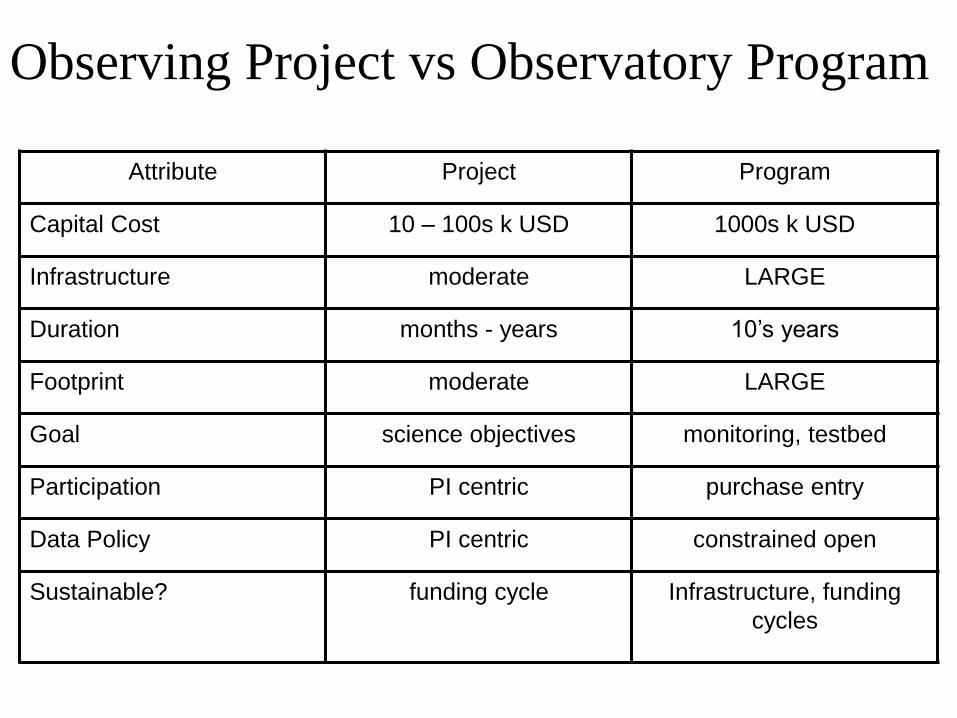
Observing Project vs Observatory Program

Attribute Project Program

Capital Cost 10 – 100s k USD 1000s k USD

Infrastructure moderate LARGE

Duration months - years 10’s years

Footprint moderate LARGE

Goal science objectives monitoring, testbed

Participation PI centric purchase entry

Data Policy PI centric constrained open

Sustainable? funding cycle Infrastructure, funding

cycles

NEPTUNE Regional ObservatoryEnvisioned circa 2001

Realized circa 2012

DEIMOS Science Objectives

63.5

cm

117 cm

61 cm

- daily vertical migrations

- predator-prey interactions (e.g. whale-krill)

- biological flux

- use of acoustics in Ocean Observatories

DEIMOS Echosounder DataFeb. 28 Mar. 1

0

875

Depth

(m

)

Time (hours)

appendicularians

(tunicates)

chaetognaths

(arrow worm)

chaetognaths

(arrow worm)

myctophids

200

250

400

300

0 m

euphausiids (krill)

Poeobius (polychaete worm)

Acanthamunnopsis

(isopod)

myctophids

Solmissus

(jellyfish)

rocketship

calycophorans

(siphophore)

Poeobius (polychaete

worm) squid

ROV dive data May 6, 2009 Bruce Robison, MBARI

Composition of Backscatter Layers

Data Volume

Monterey Data (1 frequency, 0.2 Hz sampling rate):

365 d x 24 h x 60 m x 12 pings/h x 875 m / 0.5 m resolution

How to characterize distribution patterns for data analysis

(and avoid data bottlenecks)?

= 1.104 x 1010 data points

Echometrics: Distribution

Characterization

where: sv volume backscattering coefficient, z depth, H total water column depth

Urmy et al.

2012

Quantity Metric Formula

Density Mean volume

backscattering strength10 × 𝑙𝑜𝑔10(

𝑠𝑣 𝑧 𝑑𝑧

𝐻)

Location Center of mass 𝑧 𝑠𝑣 𝑧 𝑑𝑧

𝑠𝑣 𝑧 𝑑𝑧

Dispersion Inertia 𝐶𝑀 − 𝑧 2𝑠𝑣 𝑧 𝑑𝑧

𝑠𝑣 𝑧 𝑑𝑧

Occupied Area Proportion occupied 𝑧|𝑠𝑣 𝑧 > 𝑠𝑣,𝑡ℎ𝑟𝑒𝑠ℎ𝑑𝑣

𝐻

Evenness Equivalent area ) 𝑠𝑣 𝑧 𝑑𝑧)2

𝑠𝑣 𝑧 2𝑑𝑧

Aggregation Aggregation index 𝑠𝑣(𝑧)2𝑑𝑧

) 𝑠𝑣 𝑧 𝑑𝑧 )2

Echosystem MetricsD

ep

th (

m)

De

pth

(m

)

Time (s) Time (s)

Time (s) Time (s)

De

pth

(m

)D

ep

th (

m)

Density Center of Mass

Inertia Aggregation Index

Mean volume

backscattering

strength (Sv).

Units: dB re 1 m-1

Depth mean

weighted

center.

Units: m

Variance of biomass

around center of mass

Units: m2

Patchiness,

on a scale of

0 to 1

Units: m-1

Structure

Function

Metric

Summary

March 2-4, 2009

Urmy et al. 2012

A Year in the Life of Monterey Bay

365 days x 8 metrics

= 2,920 data points

Digital Year in the Life of Monterey Bay

Data volume reduction:

7 orders of magnitude

Volume Density

Center of

Mass

Inertia

%

Occupied

Evenness

Index of

Aggregation

# Layers

Areal Density

10 min bins for daily

average

Marine Renewable Energy

Offshore Wind Surface Wave Tidal Turbine

MRE Factoids

- global consumption 15 TW (Arbic and Garrett 2010)

- current 70% of US electricity demand met by fossil fuels

- 0.3 TW global hydroelectric electricity production

- Potential: worldwide tidal dissipation 3.7 TW

- Condition: min 2 m/s tidal speed

“Environmental effects of tidal devices as one of top three

barriers to development” (Bedard 2008)

Biological Monitoring

Evolution of Perception:

Impact on devices to impact of devices

Research Needs:

who to monitor, what technologies to use, what metrics

to measure, when and where to sample, how to model

pattern, what covariates matter, how to interpret data

Evaluation:

Quantify and compare variance in density distributions

relative to baseline

Who/What to Monitor

Pilot Scale Commercial Scale

Significance: green=low, red = high

Uncertainty: 1 green =low; 2 yellow moderate; 3 red = high

Polagye et al. 2011

Site Characteristics & Sampling Decisions

Site Characteristics: high flow environments; little

previous biological sampling

Field: instrument choice & deployment, sample duty

cycle

Analytic: modeling, detecting change, identifying

causes of change, determining impacts

Applications: scaling up results from samples to site

Bottom Instrument PackagesMultibeam sonar: RESON 7128

Splitbeam echosounder:

Biosonics 120 kHz

Acoustic camera:

SoundMetrics DIDSON

Acoustic Doppler Current

Profiler: Nortek

Hydrophone,

CTD, CPOD

Survey Design: Surface

- 2 weeks May, 2 weeks June

- day, dusk (drift), night surveys

- 2 grids: north south

- midwater trawls when possible (1 knt)

- sample north or south grids on

consecutive days to cover all tidal

stages x time of day

- before, during, after bottom package deployment

- cycles: lunar, tidal, diel

- animal behavior: day, dusk, night samples

- spatial variability: representative spot, site characterization

Acoustic, midwater trawl, seabird, marine mammal surveys

Mobile Survey Stationary Survey

North GridSouth Grid

Metric Value Comparison

Scaling Up: Representative Ranges

What does a single point represent in space?

Stationary Metrics: Covariates

Metric Values Tidal Speed Time Of DayTidal Range

mean 2 std. dev.

Modeling Metric Patterns

Model Form Parametric/

Nonparametric

Variance Includes

Autocorrelation?

Error

Distribution

Linear Regression Linear Parametric Observation error only No Normal

Generalized Least Squares

(GLS)

Linear Parametric Observation error only In correlation structure Normal

Generalized Linear Model

(GLM)

Linear Parametric Observation error only No Exponential family

Generalized Linear Mixed

Model (GLMM)

Linear Parametric Observation error only In correlation structure Exponential family

Generalized Additive Model

(GAM)

Non-linear Semi-parametric Observation error only No Exponential family

Generalized Additive Mixed

Model (GAMM)

Non-linear Semi-parametric Observation error only In correlation structure Exponential family

Multivariate Auto-Regressive

State-Space (MARSS)

Linear Parametric Observation and process error Yes Normal

Auto-Regressive Integrated

Moving Average (ARIMA)

Linear Parametric Process error and observation

error

Yes Normal

ARIMA + Generalized Auto-

Regressive Conditional

Heteroskedasticity (GARCH)

Linear Parametric Process error and observation

error

Yes Generalized extensions of

normal

Random Forest N/A Non-parametric N/A Yes- lagged variables None

Support Vector Regression N/A Non-parametric N/A Yes- lagged variables None

Scenarios of Change

Stressor

Noise

Static

Device

Static

Device

Dynamic

Chemical

Spill

Change

Step

Linear

Nonlinear

Periodic

Step + Nonlinear

Effect Size

•10%

•25%

•2SD

Lag

•No lag

•1 year

Signal-to-Noise Ratio

•Initial values of error

•High error

•Low error

What Constitutes Change?

Change: deviation from a reference

Challenge: How to choose a reference/threshold?

Objective Threshold: Extreme Value Analysis

- rare but important events, high risk

- can have large impacts (e.g. 100 year flood)

Extreme Value AnalysisExtreme Value Analysis (EVA) models rare values in distribution tails.

Peaks-Over-Threshold defines extreme values above threshold. Fits

Generalized Pareto Distribution (GPD) to extreme values.

GPD

Threshold

EVA of Baseline Tidal Turbine Site

Data

Confidence Levels of Return Levels

Return Levels are average periods of extreme values + Bayesian Confidence Intervals.

Wiesebron et al. 2016a

- quantifies baseline, variability, and impacts

- site evaluation, pilot project, commercial scale

- monitoring density of instrumentation packages

- enables comparison within and among sites

- developers and regulator common language

- all marine renewable technologies

- ocean observing and environmental monitoring

Significance and Applications

Scaling

Spatial Temporal

Sensitivity Effort

Data Acquisition

Strategy

Sampling

Monitoring

Threshold

Impact

Model