BAMA01 09/03/2009 16:31 Page ii

BIOINFORMATICS AND MOLECULAR EVOLUTION

BAMA01 09/03/2009 16:31 Page i

BAMA01 09/03/2009 16:31 Page ii

Bioinformatics and Molecular Evolution

Paul G. Higgs and Teresa K. Attwood

BAMA01 09/03/2009 16:31 Page iii

© 2005 by Blackwell Science Ltda Blackwell Publishing company

BLACKWELL PUBLISHING350 Main Street, Malden, MA 02148-5020, USA108 Cowley Road, Oxford OX4 1JF, UK550 Swanston Street, Carlton, Victoria 3053, Australia

The right of Paul G. Higgs and Teresa K. Attwood to be identified as the Authors of this Work has been asserted in accordance with the UK Copyright, Designs, and Patents Act 1988.

All rights reserved. No part of this publication may be reproduced, stored in a retrieval system, or transmitted, in any form or by any means, electronic, mechanical, photocopying, recording or otherwise, except as permitted by the UK Copyright, Designs, and Patents Act 1988, without the prior permission of the publisher.

First published 2005 by Blackwell Science Ltd

Library of Congress Cataloging-in-Publication Data

Higgs, Paul G.Bioinformatics and molecular evolution / Paul G. Higgs and Teresa K. Attwood.

p. ; cm.Includes bibliographical references and index.ISBN 1–4051–0683–2 (pbk. : alk. paper)1. Molecular evolution—Mathematical models. 2. Bioinformatics.[DNLM: 1. Computational Biology. 2. Evolution, Molecular. 3. Genetics. QU 26.5 H637b 2005]

I. Attwood, Teresa K. II. Title.

QH371.3.M37H54 2005572.8—dc22

2004021066

A catalogue record for this title is available from the British Library.

Set in 91/2 /12pt Photinaby Graphicraft Limited, Hong KongPrinted and bound in the United Kingdomby TJ International, Padstow, Cornwall

The publisher’s policy is to use permanent paper from mills that operate a sustainable forestry policy, and which hasbeen manufactured from pulp processed using acid-free and elementary chlorine-free practices. Furthermore, the publisher ensures that the text paper and cover board used have met acceptable environmental accreditation standards.

For further information onBlackwell Publishing, visit our website:www.blackwellpublishing.com

BAMA01 09/03/2009 16:31 Page iv

Short Contents

Preface x

Chapter plan xiii

1 Introduction: The revolution in biological information 1

2 Nucleic acids, proteins, and amino acids 12

3 Molecular evolution and population genetics 37

4 Models of sequence evolution 58

5 Information resources for genes and proteins 81

6 Sequence alignment algorithms 119

7 Searching sequence databases 139

8 Phylogenetic methods 158

9 Patterns in protein families 195

10 Probabilistic methods and machine learning 227

11 Further topics in molecular evolution and phylogenetics 257

12 Genome evolution 283

13 DNA Microarrays and the ’omes 313

Mathematical appendix 343

List of Web addresses 355

Glossary 357

Index 363

v

BAMA01 09/03/2009 16:31 Page v

BAMA01 09/03/2009 16:31 Page vi

Full Contents

Preface x

1 INTRODUCTION: THEREVOLUTION IN BIOLOGICALINFORMATION 11.1 Data explosions 11.2 Genomics and high-throughput

techniques 51.3 What is bioinformatics? 61.4 The relationship between population

genetics, molecular evolution, andbioinformatics 7

Summary l References l Problems 10

2 NUCLEIC ACIDS, PROTEINS, AND AMINO ACIDS 122.1 Nucleic acid structure 122.2 Protein structure 142.3 The central dogma 162.4 Physico-chemical properties of the

amino acids and their importance in protein folding 222.1 Polymerase chain reaction

(PCR) 232.5 Visualization of amino acid properties

using principal component analysis 25

2.6 Clustering amino acids according to their properties 282.2 Principal component analysis

in more detail 29Summary l References l Self-testBiological background 34

3 MOLECULAR EVOLUTION ANDPOPULATION GENETICS 373.1 What is evolution? 373.2 Mutations 393.3 Sequence variation within and

between species 403.4 Genealogical trees and coalescence 443.5 The spread of new mutations 463.6 Neutral evolution and adaptation 49

3.1 The influence of selection on the fixation probability 50

3.2 A deterministic theory for the spread of mutations 51

Summary l References l Problems 54

4 MODELS OF SEQUENCEEVOLUTION 584.1 Models of nucleic acid sequence

evolution 584.1 Solution of the Jukes–Cantor

model 614.2 The PAM model of protein sequence

evolution 654.2 PAM distances 70

4.3 Log-odds scoring matrices for amino acids 71

Summary l References l Problems lSelf-test Molecular evolution 76

5 INFORMATION RESOURCES FOR GENES AND PROTEINS 815.1 Why build a database? 815.2 Database file formats 82

vii

Box

Box

Box

Box

Box

Box

BAMA01 09/03/2009 16:31 Page vii

5.3 Nucleic acid sequence databases 835.4 Protein sequence databases 895.5 Protein family databases 955.6 Composite protein pattern

databases 1085.7 Protein structure databases 1115.8 Other types of biological database 113Summary l References 115

6 SEQUENCE ALIGNMENTALGORITHMS 1196.1 What is an algorithm? 1196.2 Pairwise sequence alignment –

The problem 1216.3 Pairwise sequence alignment –

Dynamic programming methods 1236.4 The effect of scoring parameters on

the alignment 1276.5 Multiple sequence alignment 130Summary l References l Problems 136

7 SEARCHING SEQUENCEDATABASES 1397.1 Similarity search tools 1397.2 Alignment statistics (in theory) 147

7.1 Extreme value distributions 151

7.2 Derivation of the extreme value distribution in the word-matching example 152

7.3 Alignment statistics (in practice) 153Summary l References l Problems lSelf-test Alignments and database searching 155

8 PHYLOGENETIC METHODS 1588.1 Understanding phylogenetic trees 1588.2 Choosing sequences 1618.3 Distance matrices and clustering

methods 1628.1 Calculation of distances in the

neighbor-joining method 1678.4 Bootstrapping 1698.5 Tree optimization criteria and tree

search methods 171

viii

Box

Box

Box

Box

Box

Box

Box

Box

Box

8.6 The maximum-likelihood criterion 1738.2 Calculating the likelihood of

the data on a given tree 1748.7 The parsimony criterion 1778.8 Other methods related to maximum

likelihood 1798.3 Calculating posterior

probabilities 182Summary l References l Problems lSelf-test Phylogenetic methods 185

9 PATTERNS IN PROTEIN FAMILIES 1959.1 Going beyond pairwise alignment

methods for database searches 1959.2 Regular expressions 1979.3 Fingerprints 2009.4 Profiles and PSSMs 2059.5 Biological applications – G

protein-coupled receptors 208Summary l References l Problems lSelf-test Protein families and databases 216

10 PROBABILISTIC METHODS AND MACHINE LEARNING 22710.1 Using machine learning for

pattern recognition in bioinformatics 227

10.2 Probabilistic models of sequences – Basic ingredients 228

10.1 Dirichlet prior distributions 23210.3 Introducing hidden Markov models 234

10.2 The Viterbi algorithm 238

10.3 The forward and backward algorithms 239

10.4 Profile hidden Markov models 24110.5 Neural networks 244

10.4 The back-propagation algorithm 249

10.6 Neural networks and protein secondary structure prediction 250

Summary l References l Problems 253

BAMA01 09/03/2009 16:31 Page viii

13.1 Examples from the Gene Ontology 335

Summary l References l Self-test 337

MATHEMATICAL APPENDIX 343M.1 Exponentials and logarithms 343M.2 Factorials 344M.3 Summations 344M.4 Products 345M.5 Permutations and combinations 345M.6 Differentiation 346M.7 Integration 347M.8 Differential equations 347M.9 Binomial distributions 348M.10 Normal distributions 348M.11 Poisson distributions 350M.12 Chi-squared distributions 351M.13 Gamma functions and gamma

distributions 352Problems l Self-test 353

List of Web addresses 355Glossary 357Index 363

ix

Box

Box11 FURTHER TOPICS IN MOLECULAR EVOLUTION ANDPHYLOGENETICS 25711.1 RNA structure and evolution 25711.2 Fitting evolutionary models to

sequence data 26611.3 Applications of molecular

phylogenetics 272Summary l References 279

12 GENOME EVOLUTION 28312.1 Prokaryotic genomes 283

12.1 Web resources for bacterial genomes 284

12.2 Organellar genomes 298Summary l References 309

13 DNA MICROARRAYS AND THE ’OMES 31313.1 ’Omes and ’omics 31313.2 How do microarrays work? 31413.3 Normalization of microarray data 31613.4 Patterns in microarray data 31913.5 Proteomics 32513.6 Information management for

the ’omes 330

BAMA01 09/03/2009 16:31 Page ix

Preface

RATIONALE

Degree programs in bioinformatics at Masters orundergraduate level are becoming increasinglycommon and single courses in bioinformatics andcomputational biology are finding their way intomany types of degrees in biological sciences. Thisbook satisfies a need for a textbook that explains thescientific concepts and computational methods ofbioinformatics and how they relate to currentresearch in biological sciences. The content is basedon material taught by both authors on the MSc pro-gram in bioinformatics at the University of Man-chester, UK, and on an upper level undergraduatecourse in computational biology taught by P. Higgsat McMaster University, Ontario.

Many fundamental concepts in bioinformatics,such as sequence alignments, searching for homolo-gous sequences, and building phylogenetic trees, arelinked to evolution. Also, the availability of completegenome sequences provides a wealth of new data forevolutionary studies at the whole-genome level, andnew bioinformatics methods are being developedthat operate at this level. This book emphasizes theevolutionary aspects of bioinformatics, and includesa lot of material that will be of use in courses onmolecular evolution, and which up to now has notbeen found in bioinformatics textbooks.

Bioinformatics chapters of this book explain theneed for computational methods in the current eraof complete genome sequences and high-through-put experiments, introduce the principal biologicaldatabases, and discuss methods used to create and

search them. Algorithms for sequence alignment,identification of conserved motifs in protein families,and pattern-recognition methods using hiddenMarkov models and neural networks are discussedin detail. A full chapter on data analysis for micro-arrays and proteomics is included.

Evolutionary chapters of the book begin with a briefintroduction to population genetics and the study of sequence variation within and between popula-tions, and move on to the description of the evolu-tion of DNA and protein sequences. Phylogeneticmethods are covered in detail, and examples aregiven of application of these methods to biologicalquestions. Factors influencing evolution at the levelof whole genomes are also discussed, and methodsfor the comparison of gene content and gene orderbetween species are presented.

The twin themes of bioinformatics and molecularevolution are woven throughout the book – see theChapter Plan diagram below. We have consideredseveral possible orders of presenting this material,and reviewers of this book have also suggested theirown alternatives. There is no single right way to doit, and we found that no matter in which order wepresented the chapters, there was occasionally needto forward-reference material in a later chapter. Thisorder has been chosen so as to emphasize the linksbetween the two themes, and to proceed from back-ground material through standard methods to moreadvanced topics. Roughly speaking, we would con-sider everything up to the end of Chapter 9 as fun-damental material, and Chapters 10–13 as moreadvanced methods or more recent applications.

x

BAMA01 09/03/2009 16:31 Page x

Individual instructors are free to use any combina-tion of chapters in whichever order suits them best.

This book is for people who want to understandbioinformatics methods and who may want to go onto develop methods for themselves. Intelligent use ofbioinformatics software requires a proper under-standing of the mathematical and statistical meth-ods underlying the programs. We expect that manyof our readers will be biological science students whoare not confident of their mathematical ability. Wetherefore try to present mathematical material care-fully at an accessible level. However, we do not avoidthe use of equations, since we consider the theoret-ical parts of the book to be an essential aspect. Moredetailed mathematical sections are placed in boxesaside from the main text, where appropriate. Thebook contains an appendix summarizing the back-ground mathematics that we would hope bioin-formatics students should know. In our experience,students need to be encouraged to remember andpractice mathematical techniques that they havebeen taught in their early undergraduate years buthave not had occasion to use.

We discuss computational algorithms in detailbut we do not cover programming languages or pro-gramming methods, since there are many otherbooks on computing. Although we give some poin-ters to available software and useful Web sites, thisbook is not simply a list of programs and URLs. Suchmaterial becomes out of date extremely quickly,

whereas the underlying methods and principles thatwe focus on here retain their relevance.

Features

• Comprehensive coverage of bioinformatics in asingle text, including sequence analysis, biologicaldatabases, pattern recognition, and applications togenomics, microarrays, and proteomics.• Places bioinformatics in the context of evolution-ary biology, giving detailed treatments of molecularevolution and molecular phylogenetics and dis-cussing evolution at the whole-genome level.• Emphasizes the theoretical and statistical methodsused in bioinformatics programs in a way that isaccessible to biological science students.• Extended problem questions provide reinforcementof concepts and application of chapter material.• Periodic cumulative “self-tests” challenge the stu-dents to synthesize and apply their overall under-standing of the material up to that point.• Accompanied by a dedicated Web site at www.blackwellpublishing.com/higgs including thefollowing:

– all art in downloadable JPEG format (also avail-able to instructors on CD-ROM)– all answers to self-tests– downloadable sequences– links to Web resources.

xi

BAMA01 09/03/2009 16:31 Page xi

ACKNOWLEDGMENTSWe wish to thank Andy Brass for his tremendousinput to the Manchester Bioinformatics MSc pro-gram over many years, and for his “nose” for whichsubjects are the important ones to teach. We thankMagnus Rattray for his help on the theory and algo-rithms module and for coming up with several of theproblem questions in this book. Thanks are also dueto several members of our research groups whosework has helped with some of the topics coveredhere: Vivek Gowri-Shankar, Daniel Jameson, HowsunJow, Bin Tang, and Anna Gaulton.

At Blackwell publishers, we would like to thankLiz Marchant, from the UK office, who originallycommissioned this book, and Elizabeth Wald andNancy Whilton at the US office, who have givenadvice and support in the later stages.

Paul Higgs would also like to thank the enlight-ened administrative authorities at the University ofManchester for employing a physicist in the biologydepartment and the equally enlightened represent-atives of McMaster University for employing a bio-informatician in the physics department. The jumpbetween disciplines and between institutions is nottoo much of a stretch:

M--CMASTER

MANCHESTER

Paul HiggsTerri Attwood

May 2004

xii

BAMA01 09/03/2009 16:31 Page xii

xiii

Bioinformatics and Molecular EvolutionChapter Plan

1 Introduction: The Revolutionin Biological Information

2 Nucleic Acids, Proteins,and Amino Acids

3 Molecular Evolutionand Population Genetics

4 Models ofMolecular Evolution

8 Phylogenetic Methods

11 Further Topics in MolecularEvolution and Phylogenetics

12 Genome Evolution

5 Information Resourcesfor Genes and Proteins

6 Sequence AlignmentAlgorithms

7 Searching SequenceDatabases

9 Patterns inProtein Families

13 DNA Microarraysand the 'Omes

MOLECULAR EVOLUTIONTHEME

BIOINFORMATICS METHODSTHEME

10 Probablistic Methodsand Machine Learning

BAMA01 09/03/2009 16:31 Page xiii

BAMA01 09/03/2009 16:31 Page xiv

Introduction: The revolution in biologicalinformation

publicly, and freely, accessibleand that it can be retrieved and used by other researchersin the future. Most scientificjournals require submission ofnewly sequenced DNA to oneof the public databases before a publication can be made that relies on the sequence.This policy has proved tremen-dously successful for the pro-

gress of science, and has led to a rapid increase in thesize and usage of sequence databases.

As a measure of the rapid increase in the totalavailable amount of sequence data, Fig. 1.1 andTable 1.1 show the total length of all sequences inGenBank, and the total number of sequences inGenBank as a function of time. Note that the verticalscale is logarithmic and the curves appear approx-imately as straight lines. This means that the size ofGenBank is increasing exponentially with time (seeProblem 1.1). The dotted line in the figure is astraight-line fit to the data for the total sequencelength (the 1982 point seemed to be an outlier andwas excluded). From this we can estimate that theyearly multiplication factor (i.e., the factor by whichthe amount of data goes up each year) is about 1.6,and that the database doubles in size every 1.4years. All those sequencing machines are workinghard! Interestingly, the curve for the number ofsequences almost exactly parallels the curve for thetotal length. This means that the typical length ofone sequence entry in GenBank has remained at

Introduction: The revolution in biological information l 1

CHAPTER

1

1.1 DATA EXPLOSIONS

In the past decade there has been an explosion in theamount of DNA sequence data available, due to thevery rapid progress of genome sequencing projects.There are three principal comprehensive databasesof nucleic acid sequences in the world today.• The EMBL (European Molecular Biology Laborat-ory) database is maintained at the European Bioin-formatics Institute in Cambridge, UK (Stoesser et al.2003).• GenBank is maintained at the National Center for Biotechnology Information in Maryland, USA(Benson et al. 2003).• The DDBJ (DNA Databank of Japan) is maintainedat the National Institute of Genetics in Mishima,Japan (Miyazaki et al. 2003).These three databases share information and hencecontain almost identical sets of sequences. Theobjective of these databases is to ensure that DNAsequence information is stored in a way that is

CHAPTER PREVIEWHere we consider the rapid expansion in the amount of biological sequence dataavailable and compare this to the exponential growth in computer speed andmemory size that has occurred in the same period. The reader should appreciatewhy bioinformatics is now essential for understanding the information con-tained in the sequences, and for efficient storage and retrieval of the informa-tion. We also consider some of the history of bioinformatics, and show thatmany of its foundations are related to molecular evolution and populationgenetics. Thus, the reader should understand what is meant by the term “bioin-formatics” and the role of bioinformatics in relation to other disciplines.

BAMC01 09/03/2009 16:44 Page 1

close to 1000. There are, of course, enormous vari-ations in length between different sequence entries.

There is another famous exponentially increasingcurve that goes by the name of Moore’s law. Moore(1965) noticed that the number of transistors inintegrated circuits appeared to be roughly doublingevery year over the period 1959–65. Data on thesize of Intel PC chips (Table 1.2) show that this exponential increase is still continuing. Looking atthe data more carefully, however, we see that theestimate of doubling every year is rather overoptim-istic. The chip size is actually doubling every twoyears and the yearly multiplication factor is 1.4.Although extremely impressive, this is substantiallyslower than the rate of increase of GenBank (see Fig.1.1 and Table 1.3).

What about the world’s fastest supercomputers?Jack Dongarra and colleagues from the University ofTennessee introduced the LINPACK benchmark,which measures the speed of computers at solving acomplex set of linear equations. A list of the top 500supercomputers according to this benchmark ispublished twice yearly (http://www.top500.org).Figure 1.2 shows the performance benchmark rateof the top computer at each release of the list. Onceagain, this is approximately an exponential (withlarge fluctuations). The best-fit straight line has a

2 l Chapter 1

1 × 108

1 × 106

10 000

1001970 1980 1990

Year2000 2010

Total sequence length (kbp)Number of sequencesMoore's lawExponential growth

Fig. 1.1 Comparison of the rate ofgrowth of the GenBank sequence (datafrom Table 1.1) with the rate of growthof the number of transistors in personalcomputer chips (Moore’s law: datafrom Table 1.2). Dashed lines are fits to an exponential growth law.

Year Base pairs Sequences

1982 680,338 6061983 2,274,029 2,4271984 3,368,765 4,1751985 5,204,420 5,7001986 9,615,371 9,9781987 15,514,776 14,5841988 23,800,000 20,5791989 34,762,585 28,7911990 49,179,285 39,5331991 71,947,426 55,6271992 101,008,486 78,6081993 157,152,442 143,4921994 217,102,462 215,2731995 384,939,485 555,6941996 651,972,984 1,021,2111997 1,160,300,687 1,765,8471998 2,008,761,784 2,837,8971999 3,841,163,011 4,864,5702000 11,101,066,288 10,106,0232001 15,849,921,438 14,976,3102002 28,507,990,166 22,318,883

Data obtained from http://www.ncbi.nih.gov/Genbank/genbankstats.html.

Table 1.1 The growth of GenBank.

BAMC01 09/03/2009 16:44 Page 2

doubling time of 1.04 years. So supercomputersseem to be beating GenBank for the moment.However, most of us do not have access to a super-computer. The PC chip size may be a better measureof the amount of computing power available to any-one using a desktop.

Clearly, we have reached a point where com-puters are essential for the storage, retrieval, andanalysis of biological sequence data. However, wecannot simply rely on computers and stop thinking.If we stick with our same old computing methods,then we will be limited by the hardware. We still

need people, because only people can think of betterand faster algorithms for data analysis. That is whatthis book is about. We will discuss the methods andalgorithms used in bioinformatics, so that hopefullyyou will understand enough to be able to improvethose methods yourself.

Another important type of biological data that isexponentially increasing is protein structures. PDBis a database of protein structures obtained from X-ray crystallography and NMR experiments. Fromthe number of entries in PDB in successive releases,we calculated that the doubling time for the number

Introduction: The revolution in biological information l 3

Type of processor Year of introduction Transistors

4004 1971 2,2508008 1972 2,5008080 1974 5,0008086 1978 29,000286 1982 120,000386™ processor 1985 275,000486™ DX processor 1989 1,180,000Pentium® processor 1993 3,100,000Pentium II processor 1997 7,500,000Pentium III processor 1999 24,000,000Pentium 4 processor 2000 42,000,000

Data obtained from Intel(http://www.intel.com/research/silicon/mooreslaw.htm).

Table 1.2 The growth of the numberof transistors in personal computerprocessors.

10 000

1000

1001994 19981996 2000

Year2002 2004

Benchmark rate (Gflops)Exponential growth

Fujitsu Numerical Wind TunnelHitachi SR2201/1024

Hitachi/Tsukuba CP-PACS/2048

Intel ASCI Red

Intel ASCI Red

Intel ASCI Red

IBM ASCI White

IBM ASCI White

NEC Earth Simulator

Fig. 1.2 The performance of theworld’s top supercomputers using theLINPACK benchmark (Gflops). Datafrom http://www.top500.org.

BAMC01 09/03/2009 16:44 Page 3

of available protein structures is 3.31 years (Table1.3), which is considerably slower than the numberof sequences. Since the number of experimentallydetermined structures is lagging further and furtherbehind the number of sequences, computationalmethods for structure prediction are important.Many of these methods work by looking for similar-ities in sequence between a protein of unknownstructure and a protein of known structure, and usethis to make predictions about the unknown struc-ture. These techniques will become increasinglyuseful as our knowledge of real examples increases.

In 1995, the bacterium Haemophilus influenzae en-tered history as the first organism to have its genomecompletely sequenced. Sequencing technology has

advanced rapidly and has become increasingly auto-mated. The sequencing of a new prokaryotic genomehas now become almost commonplace. Table 1.4shows the progress of complete genome projects withsome historical landmarks. With the publication ofthe human genome in 2001, we can now truly saythat we are in the “post-genome age”. The numberof complete prokaryotic genomes (total of archaeaplus bacteria from Table 1.4) is going through itsown data explosion. The doubling time is about 1.3years and the yearly multiplication factor is about1.7. For the present, complete eukaryotic genomesare still rather few, so that the publication of eachindividual genome still retains its status as a land-mark event. It seems only a matter of time, however,

4 l Chapter 1

Type of data Growth rate, r Doubling time, Yearly multiplication T (years) factor, R

GenBank (total sequence length) 0.480 1.44 1.62PC chips (number of transistors) 0.332 2.09 1.39Supercomputer speed (LINPACK benchmark) 0.664 1.04 1.94Protein structures (number of PDB entries) 0.209 3.31 1.23Number of complete prokaryotic genomes 0.518 1.34 1.68Abstracts: bioinformatics 0.587 1.18 1.80Abstracts: genomics 0.569 1.22 1.77Abstracts: proteomics 0.996 0.70 2.71Abstracts: phylogenetic(s) 0.188 3.68 1.21Abstracts: total 0.071 9.80 1.07

Table 1.3 Comparison of rates of increase of several different data explosion curves.

Year Archaea Bacteria Eukaryotes Landmarks

1995 0 2 0 First bacterial genome: Haemophilus influenzae1996 1 2 0 First archaeal genome: Methanococcus jannaschii1997 2 4 1 First unicellular eukaryote: Saccharomyces cerevisiae1998 1 5 1 First multicellular eukaryote: Caenorhabditis elegans1999 1 4 1 —2000 3 13 2 First plant genome: Arabidopsis thaliana2001 2 24 3 First release of the human genome2002 6 32 9 —2003 (to July) 0 25 2 —Total 16 111 19 —

Data from the Genomes OnLine Database (http://wit.integratedgenomics.com/GOLD/).

Table 1.4 The history of genome-sequencing projects.

BAMC01 09/03/2009 16:44 Page 4

before we shall be able to draw a data explosioncurve for the number of eukaryotic genomes too.

This book emphasizes the relationship betweenbioinformatics and molecular evolution. The avail-ability of complete genomes is tremendously import-ant for evolutionary studies. For the first time we can begin to compare whole sets of genes betweenorganisms, not just single genes. For the first time we can begin to study the processes that govern theevolution of whole genomes. This is therefore anexciting time to be in the bioinformatics area.

1.2 GENOMICS AND HIGH-THROUGHPUT TECHNIQUES

The availability of complete genomes has opened upa whole research discipline known as genomics.Genomics refers to scientific studies dealing withwhole sets of genes rather than single genes. Theadvances made in sequencing technology havecome at the same time as the appearance of newhigh-throughput experimental techniques. One ofthe most important of these is microarray techno-logy, which allows measurement of the expressionlevel (i.e., mRNA concentration) of thousands ofgenes in a cell simultaneously. For example, in thecase of the yeast, Saccharomyces cerevisiae, where thecomplete genome is available, we can put probes forall the genes onto one microarray chip. We can thenstudy the way the expression levels of all the genesrespond to changes in external conditions or theway that they vary during the cell cycle. Completegenomes therefore change the way that experimen-tal science is carried out, and allow us to addressquestions that were not possible before.

Another important field where high-throughputtechniques are used is proteomics. Proteomics isthe study of the proteome, i.e., the complete set ofproteins in a cell. The experimental techniques usedare principally two-dimensional gel electrophoresisfor the separation of the many different proteins in acell extract, and mass spectrometry for identifyingproteins by their molecular masses. Once again, theavailability of complete genomes is tremendouslyimportant, because the masses of the proteins deter-

mined by mass spectrometry can be compareddirectly to the masses of proteins expected from thepredicted position of open reading frames in thegenome.

High-throughput experiments produce largeamounts of quantitative data. This poses challengesfor bioinformaticians. How do we store informationfrom a microarray experiment in such a way that itcan be compared with results from other groups?How do we best extract meaningful informationfrom the vast array of numbers generated? New statistical methods are needed to spot significanttrends and patterns in the data. This is a new area ofbiological sciences where computational methodsare essential for the progress of the experimental science, and where algorithms and experimentaltechniques are being developed side by side.

As a measure of the interest of the scientific com-munity in genomics and related areas, let us look atthe number of scientific papers published in theseareas over the past few years. The ISI ScienceCitation Index allows searches for articles publishedin specific years that use specified words in their title,keywords, or abstract. Figure 1.3 shows the num-bers of published articles (cumulative since 1981)for several important terms relevant to this book.Papers using the words “genomics” and “bioinform-atics” increase at almost exactly the same rate, both having yearly multiplication factors of 1.8 anddoubling times of 1.2 years. “Proteomics” is a veryyoung field, with no articles found prior to 1998.The doubling time is 0.7 years: the fastest growth ofany of the quantities considered in Table 1.3.References to “microarray” also increase rapidly.This curve appears significantly nonlinear becausethere are several different meanings for the term.Almost all the references prior to about 1996 refer tomicroarray electrodes, whereas in later years,almost all refer to DNA microarrays for gene expres-sion. The rate of increase of the use of DNA microar-rays is therefore steeper than it appears in the figure.

The number of papers using both “sequence” and“database” is much larger than those using any of theterms considered above (although it is increasing lessrapidly). This shows how important biological data-bases and the algorithms for searching them have

Introduction: The revolution in biological information l 5

BAMC01 09/03/2009 16:44 Page 5

become to the biological science community in thepast decade. The number of papers using the term“phylogenetic” or “phylogenetics” dwarfs those usingall the other terms considered here by at least anorder of magnitude. This curve is a remarkably goodexponential, although the doubling time is fairly long(3.7 years). Phylogenetics is a relatively old area,where morphological studies predate the availabil-ity of molecular sequences by several decades. Thehigh level of interest in the field in recent years islargely a result of the availability of sequence dataand of new methods for tree construction. Very largesequence data sets are now being used, and we arebeginning to resolve some of the controversialaspects of evolutionary trees that have been arguedover for decades.

As a comparison, for all the curves in Fig. 1.3 thatrefer to specific scientific terms, the figure also showsthe total number of articles in the Science CitationIndex (this curve is in millions of articles, whereasthe others are in individual articles). The total levelof scientific activity (or at least, scientific writing)has also been increasing exponentially, and hencewe all have to read more and more in order to keepup. This curve is an almost perfect exponential, witha doubling time of 9.8 years. Thus, all the curvesrelated to the individual subjects are increasing farmore rapidly than the total accumulation of sci-entific knowledge.

At this point you will be suitably impressed by theimportance of the subject matter of this book andwill be eager to read the rest of it!

1.3 WHAT IS BIOINFORMATICS?

Since bioinformatics is still a fairly new field, peoplehave a tendency to ask, “What is bioinformatics?”Often, people seem to worry that it is not very welldefined, and tend to have a suspicious look in theireyes when they ask. These people would never trou-ble to ask “What is biology?” or “What is genetics?”In fact, bioinformatics is no more difficult or moreeasy to define than these other fields. Here is ourshort and simple definition.

Bioinformatics is the use of computational meth-ods to study biological data.

In case this is too short and too general for you, hereis a longer one.

Bioinformatics is:(i) the development of computational methods forstudying the structure, function, and evolution ofgenes, proteins, and whole genomes;(ii) the development of methods for the manage-ment and analysis of biological information arisingfrom genomics and high-throughput experiments.

6 l Chapter 1

10 000

1000

100

10

1994 1996 1998Year

2000 2002 2004

GenomicsProteomicsMicroarrayBioinformaticsPhylogenetic(s)Sequence AND databaseTotal (in millions)

Num

ber

of a

rtic

les

Fig. 1.3 Cumulative number of scientific articles published from 1981to the date shown that use specific terms in the title, keywords, or abstract.Data from the Science Citation Index(SCI-EXPANDED) available at http://wos.mimas.ac.uk/ orhttp://isi6.isiknowledge.com.

BAMC01 09/03/2009 16:44 Page 6

If that is still too short, have another look at the con-tents list of this book to see what we think are themost important topics that make up the field ofbioinformatics.

1.4 THE RELATIONSHIP BETWEENPOPULATION GENETICS, MOLECULAREVOLUTION, AND BIOINFORMATICS

1.4.1 A little history . . .

The field of population genetics is concerned withthe variation of genes within a population. Theissues of natural selection, mutation, and ran-dom drift are fundamental to population genetics.Alternative versions of a gene are known as alleles.A large body of population genetics theory is used tointerpret experimental data on allele frequency dis-tributions and to ask questions about the behavior ofthe organisms being studied (e.g., effective popula-tion size, pattern of migration, degree of inbreeding).Population genetics is a well-established disciplinewith foundations dating back to Ronald Fisher andSewall Wright in the first half of the twentieth cen-tury. These foundations predate the era of molecularsequences. It is possible to discuss the theory of thespread of a new allele, for example, without knowinganything about its sequence.

Molecular evolution is a more recent disciplinethat has arisen since DNA and protein sequenceinformation has become available. Molecular tech-niques provide many types of data that are of greatuse to population geneticists, e.g., allozymes, micro-satellites, restriction fragment length polymorph-isms, single nucleotide polymorphisms, humanmitochondrial haplotypes. Population geneticistsare interested in what these molecular markers tellus about the organisms (see the many examples inthe book by Avise 1994). In contrast, the focus ofmolecular evolution is on the molecules themselves,and understanding the processes of mutation andselection that act on the sequences. There are manygenes that have now been sequenced in a largenumber of different species. This usually means thatwe have a representative example of a single genesequence from each species. There are only a few

species for which a significant amount of informationabout within-species sequence variation is available(e.g., humans and Drosophila). The emphasis inmolecular evolution therefore tends to be on com-parative molecular studies between species, whilepopulation genetics usually considers variationwithin a species.

The article by Zuckerkandl and Pauling (1965) is sometimes credited with inventing the field ofmolecular evolution. This was the first time that pro-tein sequences were used to construct a molecularphylogeny and it set many people thinking aboutbiological sequences in a quantitative way. 1965was the same year in which Moore invented his lawand in which computers were beginning to play asignificant role in science. Indeed, molecular biologyhas risen to prominence in the biological sciences inthe same time frame that computers have risen toprominence in society in general.

We might also argue that bioinformatics wasbeginning in 1965. The first edition of the Atlas ofProtein Sequence and Structure, compiled by MargaretDayhoff, appeared in printed form in 1965. TheAtlas later became the basis for the PIR proteinsequence database (Wu et al. 2002). However, this isstretching the point a little. The term bioinformaticswas not around in 1965, and barring a few pioneers,bioinformatics was not an active research area atthat time. As a discipline, bioinformatics is morerecent. It arose from the recognition that efficientcomputational techniques were needed to study thehuge amount of biological sequence informationthat was becoming available. If molecular biologyarose at the same time as scientific computing, thenwe may also say that bioinformatics arose at thesame time as the Internet. It is possible to imaginethe existence of biological sequence databases with-out the Internet, but they would be a whole lot lessuseful. Database use would be restricted to those whosubscribed to postal deliveries of database releases.Think of that cardboard box arriving each monthand getting exponentially bigger each time. AmosBairoch of the Swiss Institute of Bioinformatics com-ments (Bairoch 2000) that in 1988, the version oftheir PC/Gene database and software was shipped as53 floppy disks! For that matter, think how difficult it

Introduction: The revolution in biological information l 7

BAMC01 09/03/2009 16:44 Page 7

would be to submit sequences to a database if it werenot for email and the Internet.

At this point, the first author of this book starts tofeel old. Coincidentally, I also first saw the light ofday in 1965. Shortly afterwards, in 1985, I was hap-pily writing programs with DO-loops in them formainframes (students who are too young to knowwhat mainframe computers are probably do notneed to know). In 1989, someone first showed mehow to use a mouse. I remember this clearly becauseI used the mouse for the first time when I began towrite my Ph.D. thesis. It is scary to think almost allmy education is pre-mouse. Possibly even morefrightening is that I remember – it must have been in1994 – someone explaining to our academic depart-ment how the World-Wide Web worked and whatwas meant by the terms URL and Netscape. A yearor so after that, use of the Internet had become adaily affair for me. Now, of course, if the network isdown for a day, it is impossible to do anything at all!

1.4.2 Evolutionary foundations for bioinformatics

Let’s get back to the plot. Bioinformatics is a new dis-cipline. Since this is a bioinformatics book, why dowe need to know about the older subjects of mole-cular evolution and population genetics? There is a famous remark by the evolutionary biologistTheodosius Dobzhansky that, “Nothing in biologymakes sense except in the light of evolution”. Youwill find this quoted in almost every evolutionarytextbook, but we will not apologize for quoting itonce again. In fact, we would like to update it to,“Nothing in bioinformatics makes sense except inthe light of evolution”. Let’s consider some examplesto see why this is so.

The most fundamental and most frequently usedprocedure in bioinformatics is pairwise sequencealignment. When amino acid sequences are aligned,we use a scoring system, such as a PAM matrix, todetermine the score for aligning any amino acidwith any other. These scoring systems are based on evolutionary models. High scores are assigned to pairs of amino acids that frequently substitute for one another during protein sequence evolution.Low, or negative, scores are assigned to pairs of

amino acids that interchange very rarely. WhenRNA sequences are aligned, we often use the factthat the secondary structure tends to be conserved,and that pairs of compensatory substitutions occurin the base-paired regions of the structure. Thus,creating accurate sequence alignments of both pro-teins and RNAs relies on an understanding of mole-cular evolution.

If we want to know something about a particularbiological sequence, the first thing we do is searchthe database to find sequences that are similar to it.In particular, we are often interested in sequencemotifs that are well conserved and that are presentin a whole family of proteins. The logic is that im-portant parts of a sequence will tend to be conser-ved during evolution. Protein family databases likePROSITE, PRINTS, and InterPro (see Chapter 5)identify important conserved motifs in protein align-ments and use them to assign sequences to families.An important concept here is homology. Sequencesare homologous if they descend from a commonancestor, i.e., if they are related by the evolutionaryprocess of divergence. If a group of proteins all sharea conserved motif, it will often be because all theseproteins are homologous. If a motif is very short,however, there is some chance that it will haveevolved more than once independently (conver-gent evolution). It is therefore important to try todistinguish chance similarities arising from con-vergent evolution from similarities arising fromdivergent evolution. The thrust of protein familydatabases is therefore to facilitate the identificationof true homologs, by making the distinction betweenchance and real matches clearer.

Similar considerations apply in protein structuraldatabases. It is often observed that distantly relatedproteins have relatively conserved structures. Forexample, the number and relative positions of αhelices and β strands might be the same in two pro-teins that have very different sequences. Occasion-ally, the sequences are so different that it would bevery difficult to establish a relationship between themif the structure were not known. When similar (oridentical) structures are found in different proteins,it probably indicates homology, but the possibility ofsmall structural motifs arising more than once still

8 l Chapter 1

BAMC01 09/03/2009 16:44 Page 8

needs to be considered. Another important aspect ofprotein structure that is strongly linked to evolutionis domain shuffling. Many large proteins are com-posed of smaller domains that are continuous sec-tions of the sequence that fold into fairly well-definedthree-dimensional structures; these assemble toform the overall protein structure. Particularly ineukaryotes, it is found that certain domains occur inmany different proteins in different combinationsand different orders. See the ProDom database(Corpet et al. 2000), for example. Although bioin-formaticians will argue about what constitutes adomain and where the boundaries between domainslie, it is clear that the duplication and reshuffling ofdomains is a very useful way of evolving new com-plex proteins. The main message is that in order tocreate reliable information resources for proteinsequences, structures, and domains, we need tohave a good understanding of protein evolution.

In recent years, evolutionary studies have alsobecome possible at the whole genome level. If wewant to compare the genomes of two species, it isnatural to ask which genes are shared by bothspecies. This question can be surprisingly hard toanswer. For each gene in the first species, we need todecide if there is a gene in the second species that ishomologous to it. It may be difficult to detect similar-ity between sequences from different species simplybecause of the large amount of evolutionary changethat has gone on since the divergence of the species.Most genomes contain many open reading framesthat are thought to be genes, but for which no sim-ilar sequence can be found in other species. This isevidence for the limitations of our current methodsas much as for the diversity generated by molecularevolution. In cases where we are able to detect sim-ilarity, then it can still be tough to decide which genesare homologous. Many genomes contain families ofduplicated genes that often have slightly differentfunctions or different sites of expression within theorganism. Sequences from one species that are evo-lutionarily related and that diverged from oneanother due to a gene duplication event are calledparalogous sequences, in contrast to orthologoussequences, which are sequences in different organ-isms that diverged from one another due to the split

between the species. Duplications can occur in dif-ferent lineages independently, so that a single genein one species might be homologous to a whole fam-ily in the other species. Alternatively, if duplicationsoccurred in a common ancestor, then both speciesshould contain a copy of each member of the genefamily – unless, of course, some genes have beendeleted in one or other species. Another factor toconsider, particularly for bacteria, is that genomescan acquire new genes by horizontal transfer of DNAfrom unrelated species. This sequence comparisoncan show up genes that are apparently homolog-ous to sequences in organisms that are otherwisethought to be extremely distantly related. A majortask for bioinformatics is to establish sets of homolog-ous genes between groups of species, and to under-stand how those genes got to be where they are. Theflip side of this is to be able to say which genes arenot present in an organism, and how the organismmanages to get by without them.

The above examples show that many of the ques-tions addressed in bioinformatics have foundationsin questions of molecular evolution. A fair amountof this book is therefore devoted to molecular evolu-tion. What about population genetics? There aremany other books on population genetics and hencethis book does not try to be a textbook of this area.However, there are some key points that are usuallyconsidered in population genetics courses that weneed to consider if we are to properly understandmolecular evolution and bioinformatics. These ques-tions concern the way in which sequence diversity isgenerated in populations and the way in which newvariant sequences spread through populations. If werun a molecular phylogeny program, for example,we might be asking whether “the” sequence fromhumans is more similar to “the” sequence from chim-panzees or gorillas. It is important to remember that these sequences have diverged as a result of thefixation of new sequence variants in the populations.We should also not forget that the sequences wehave are just samples from the variations that existin each of the populations.

There are some bioinformatics areas that have adirect link to the genetics of human populations. Weare accumulating large amounts of information

Introduction: The revolution in biological information l 9

BAMC01 09/03/2009 16:44 Page 9

about variant gene sequences in human popula-tions, particularly where these are linked to hered-itary diseases. Some of these can be major changes,like deletions of all or part of a gene or a chromosomeregion. Some are single nucleotide polymorphisms,or SNPs, where just a single base varies at a particu-lar site in a gene. Databases of SNPs potentially con-tain information of great relevance to medicine andto the pharmaceutical industry. The area of phar-macogenomics attempts to understand the waythat different patients respond more or less well to

drug treatments according to which alleles theyhave for certain genes. The hope is that drug treat-ments can be tailored to suit the genetic profile of thepatient. However, many important diseases are notcaused by a single gene. Understanding the way thatvariations at many different loci combine to affectthe susceptibility of individuals to different medicalproblems is an important goal, and developing com-putational techniques to handle data such as SNPs,and to extract information from the data, is animportant application of bioinformatics.

10 l Chapter 1

SUMMARYThe amount of biological sequence information isincreasing very rapidly and seems to be following anexponential growth law. Computational methods areplaying an increasing role in biological sciences. Newalgorithms will be required to analyze this informationand to understand what it means. Genome sequencingprojects have been remarkably successful, and compar-ative analysis of whole genomes is now possible. Thisprovides challenges and opportunities for new types ofstudy in bioinformatics. At the same time, several types of experimental methods are being developed cur-rently that may be classed as “high-throughput”. Theseinclude microarrays, proteomics, and structural gen-omics. The philosophy behind these methods is to studylarge numbers of genes or proteins simultaneously, rather

than to specialize in individual cases. Bioinformaticstherefore has a role in developing statistical methods foranalysis of large data sets, and in developing methods of information management for the new types of databeing generated.

Evolutionary ideas underlie many of the methods usedin bioinformatics, such as sequence alignments, iden-tifying families of genes and proteins, and establishinghomology between genes in different organisms. Evolu-tionary tree construction (i.e., molecular phylogenetics)is itself a very large field within computational biology.Since we now have many complete genomes, particularlyin bacteria, we can also begin to look at evolutionaryquestions at the whole-genome level. This book willtherefore pay particular attention to the evolutionaryaspects of bioinformatics.

REFERENCESAvise, J.C. 1994. Molecular Markers, Natural History, and

Evolution. New York: Chapman and Hall.Bairoch, A. 2000. Serendipity in bioinformatics: The tri-

bulations of a Swiss bioinformatician through excitingtimes. Bioinformatics, 16: 48–64.

Benson, D.A., Karsch-Mizrachi, I., Lipman, D.J., Ostell, J.,and Wheeler, D.L. 2003. GenBank. Nucleic AcidsResearch, 31: 23–7.

Corpet, F., Sernat, F., Gouzy, J., and Kahn, D. 2000.ProDom and ProDom-CG: Tools for protein domainanalysis and whole genome comparisons. Nucleic AcidsResearch, 28: 267–9. http://prodes.toulouse.inra.fr/prodom/2002.1/html/home.php

Miyazaki, S., Sugawara, H., Gojobori, T., and Tateno, Y.2003. DNA Databank of Japan (DDBJ) in XML. NucleicAcids Research, 31: 13–16.

Moore, G.E. 1965. Cramming more components onto integ-rated circuits. Electronics, 38(8): 114–17.

Stoesser, G., Baker, W., van den Broek, A., Garcia-Pastor,M., Kanz, C., Kulikova, T., Leinonen, R., Lin, Q.,Lombard, V., Lopez, R., Mancuso, R., Nardone, R.,Stoehr, P., Tuli, M.A., Tzouvara, K., and Vaughan, R.2003. The EMBL Nucleotide Sequence Database: Majornew developments. Nucleic Acids Research, 31: 17–22.

Wu, C.H., Huang, H., Arminski, L., Castro-Alvear, J.,Chen, Y., Hu, Z.Z., Ledley, R.S., Lewis, K.C., Mewes,H.W., Orcutt, B., Suzek, B.E., Tsugita, A., Vinayaka,C.R., Yeh, L.L., Zhang, J., and Barker, W.C. 2002. TheProtein Information Resource: An integrated publicresource of functional annotation of proteins. NucleicAcids Research, 30: 35–7. http://pir.georgetown.edu/.

Zuckerkandl, E. and Pauling, L. 1965. Evolutionary divergence and convergence in proteins. In V. Bryson,and H.J. Vogel (eds.), Evolving Genes and Proteins, pp. 97–166. New York: Academic Press.

BAMC01 09/03/2009 16:44 Page 10

Introduction: The revolution in biological information l 11

PROBLEMS

1.1 The data explosion curves provide us with a goodway of revising some fundamental points in mathematicsthat will come in handy later in the book. Now wouldalso be a good time to check the Mathematical appendixand maybe have a go at the Self-test that goes with it.

For each type of data considered in this chapter, wehave a quantity N(t) that is increasing with time t, andwe are assuming that it follows the law:

N(t) = N0 exp(rt)

Here, N0 is the value at the initial time point, and r is thegrowth rate. In the cases we considered, time was meas-ured in years. We defined the yearly multiplication factoras the factor by which N increases each year, i.e.

If the data really follow an exponential law, then thisratio is the same at whichever time we measure it.Another way of writing the growth law is therefore:

N(t) = N0Rt

The other useful quantity that we measured was thedoubling time T. To calculate T we require that the num-ber after a time T is twice as large as its initial value.

= exp(rT ) = 2

Hence rT = ln(2) or T = ln(2)/r.If any of these steps is not obvious, then you should

revise your knowledge of exponentials and logarithms.There are some helpful pointers in the Mathematicalappendix of this book, Section M.1.

1.2 Use the data from Tables 1.1 and 1.2 and plot yourown graphs. The figures in this chapter plot N directlyagainst t and use a logarithmic scale on the vertical axis.This comes out to be a straight line because:

ln(N) = ln(N0) + rt

so the slope of the line is r. The other way to do it is tocalculate ln(N) at each time point with a calculator, and

N TN( )

0

R

N tN t

r ( )

( ) exp( )=

+=

1

then to plot ln(N) against t using a linear scale on bothaxes. Plot the graphs both ways and make sure they lookthe same.

My graph-plotting package will do a best fit of anexponential growth law to a set of data points. This ishow the values of r were obtained in Table 1.3. However,if your package will not do that, then you can also estim-ate r from the ln(N) versus t graph by using a straight-line fit. Try doing the fit to the data in both ways andmake sure that you get the same answer.

1.3 The exponential growth law arises from the as-sumption that the rate of increase of N is proportional toits current value. Thus the growth law is the solution ofthe differential equation

Now would be a good time to make sure you under-stand what this equation means (see Sections M.6 andM.8 for some help).

1.4 While the assumption in 1.3 might have some plaus-ibility for the increase in the size of a rabbit population (if they have a limitless food supply), there does notseem to be a theoretical reason why the size of GenBankor the size of a PC chip should increase exponentially. Itis just an empirical observation that it works that way.Presumably, sooner or later all these curves will hit alimit.

There are several other types of curve we might imag-ine to describe an increasing function of time.Linear increase: N(t) = A + BtPower law increase: N(t) = Atk (for some value of k

not equal to 1)Logarithmic increase: N(t) = A + B ln(t)In each case, A, B, and k are arbitrary constants thatcould be obtained by fitting the curve to the data. Try tofit the data in Tables 1.1 and 1.2 to these other growthlaws. Is it true that the exponential growth law fits betterthan the alternatives?

If you had some kind of measurements that youbelieved followed one of the other growth laws, howwould you plot the graph so that the points would lie ona straight line?

dNdt

rN =

BAMC01 09/03/2009 16:44 Page 11

12 l Chapter 2

Nucleic acids,proteins, and amino acids

bose, but the molecules areotherwise the same.

Each sugar is linked to amolecule known as a base. InDNA, there are four types ofbase, called adenine, thymine,guanine, and cytosine, usu-ally referred to simply as A, T,G, and C. The structures ofthese molecules are shown inFig. 2.2. In RNA, the base

uracil (U; Fig. 2.2) occurs instead of T. The structureof U is similar to that of T but lacks the CH3 grouplinked to the ring of the T molecule. In addition, avariety of bases of slightly different structures, calledmodified bases, can also be found in some types ofRNA molecule. A and G are known as purines. Theyboth have a double ring in their chemical structure.C, T, and U are known as pyrimidines. They have asingle ring in their chemical structure. The funda-mental building block of nucleic acid chains is calleda nucleotide: this is a unit of one base plus one sugarplus one phosphate. We usually think of the “length”of a nucleic acid sequence as the number of nucle-otides in the chain. Nucleotides are also found asseparate molecules in the cell, as well as being part ofnucleic acid polymers. In this case, there are usuallytwo or three phosphate groups attached to the samenucleotide. For example, ATP (adenosine triphos-phate) is an important molecule in cellular metabol-ism, and it has three phosphates attached in a chain.

DNA is usually found as a double strand. The two strands are held together by hydrogen bonding

CHAPTER

2

2.1 NUCLEIC ACID STRUCTURE

There are two types of nucleic acid that are of keyimportance in cells: deoxyribonucleic acid (DNA)and ribonucleic acid (RNA). The chemical structureof a single strand of RNA is shown in Fig. 2.1. Thebackbone of the molecule is composed of ribose units(five-carbon sugars) linked by phosphate groups in a repeating polymer chain. Two repeat units areshown in the figure. The carbons in the ribose areconventionally numbered from 1 to 5, and the phos-phate groups are linked to carbons 3 and 5. At oneend, called the 5′ (“five prime”) end, the last carbonin the chain is a number 5 carbon, whereas at theother end, called the 3′ end, the last carbon is a number 3. We often think of a strand as beginning at the 5′ end and ending at the 3′ end, because this is the direction in which genetic information is read.The backbone of DNA differs in that deoxyribosesugars are used instead of ribose. The OH group oncarbon number 2 in ribose is simply an H in deoxyri-

CHAPTER PREVIEWThis chapter begins with a basic introduction to the chemical and physical structure of nucleic acids and proteins for those who do not have a backgroundin biochemistry or biology. We also give a reminder of the processes of transcrip-tion, RNA processing, translation and protein synthesis, and DNA replication.We then give a detailed discussion of the physico-chemical properties of theamino acids and their relevance in protein folding. We use the amino acid property data as an example when introducing two statistical techniques thatare useful in bioinformatics: principal component analysis and clustering algorithms.

BAMC02 09/03/2009 16:43 Page 12

between A and T and between C and G bases (Fig. 2.2). The two strands run in opposite directionsand are exactly complementary in sequence, so thatwhere one has A, the other has T and where one hasC the other has G. For example:

5′–C–C–T–G–A–T–3′3′–G–G–A–C–T–A–5′

The two strands are coiled around one another inthe famous double helical structure elucidated byWatson and Crick 50 years ago. This is shownschematically in Fig. 2.3.

In contrast, RNA molecules are usually singlestranded, and can form a variety of structures bybase pairing between short regions of complement-ary sequences within the same strand. An exampleof this is the cloverleaf structure of transfer RNA(tRNA), which has four base-paired regions (stems)and three hairpin loops (Fig. 2.4). The base-pairingrules in RNA are more flexible than DNA. The prin-cipal pairs are GC and AU (which is equivalent to ATin DNA), but GU pairs are also relatively frequent,and a variety of unusual, so-called “non-canonical”,pairs are also found in some RNA structures (e.g., GA pairs). A two-dimensional drawing of the base-pairing pattern is called a secondary structure

Nucleic acids, proteins, and amino acids l 13

CH2

OP

OH

O

O

O

5' end

CH2

–O

–O

P

OH

O

O

O

O

3' end

21

5

34

21

5

34

Base

Base

Phosphate

Ribose sugar

Fig. 2.1 Chemical structure of the RNA backbone showingribose units linked by phosphate groups.

CH3

Adenine Thymine

Guanine Cytosine

Uracil

N H

N

H

O

O

N N

NN

N NH

H

H

H O

O

NH HSugar

Sugar

N N

NN

N N

H H

H

O

O

H

NH H

H

N H

Sugar

Sugar

Fig. 2.2 The chemical structure of the four bases of DNAshowing the formation of hydrogen-bonded AT and GC basepairs. Uracil is also shown.

C

C

C

C

T

T

T

A

A

A

A

A

G

G

G

G

Major grooveMinor groove

5' 3'

5'3'

Fig. 2.3 Schematic diagram of the DNA double helical structure.

BAMC02 09/03/2009 16:43 Page 13

diagram. In Chapter 11, we will discuss RNA sec-ondary structure in more detail.

2.2 PROTEIN STRUCTURE

The fundamental building block of proteins is theamino acid. An amino acid has the chemical struc-ture shown in Fig. 2.5(a), with an amine group onone side and a carboxylic acid group on the other. Insolution, these groups are often ionized to give NH3

+

and COO−. There are 20 types of amino acid found inproteins. These are distinguished by the nature ofthe side-chain group, labeled R in Fig. 2.5(a). Thecentral carbon to which the R group is attached isknown as the α carbon. Proteins are linear polymerscomposed of chains of amino acids. The links areformed by removal of an OH from one amino acidand an H from the next to give a water molecule. The

resultant linkage is called a peptide bond. These areshown in boxes in Fig. 2.5(b), which illustrates a tripeptide, i.e., a chain composed of three aminoacids. Proteins, or “polypeptides”, are typically com-posed of several hundred amino acids.

The chemical structures of the side chains are givenin Fig. 2.6. Each amino acid has a standard three-letter abbreviation and a standard one-letter code,as shown in the figure. A protein can be representedsimply by a sequence of these letters, which is veryconvenient for storage on a computer, for example:

MADIQLSKYHVSKDIGFLLEPLQDVLPDYFAPWNR

LAKSLPDLVASHKFRDAVKEMPLLDSSKLAGYRQK

is the first part of a real protein. The two ends of aprotein are called the N terminus and the C terminusbecause one has an unlinked NH 3

+ group and theother has an unlinked COO− group. Protein sequ-ences are traditionally written from the N to the Cterminus, which corresponds to the direction inwhich they are synthesized.

The four atoms involved in the peptide bond lie ina plane and are not free to rotate with respect to oneanother. This is due to the electrons in the chemicalbonds, which are partly delocalized. The flexibility ofthe protein backbone comes mostly from rotationabout the two bonds on either side of each α carbon.Many proteins form globular three-dimensional struc-tures due to this flexibility of the backbone. Each pro-tein has a structure that is specific to its sequence.The formation of this three-dimensional structure is called “protein folding”. The amino acids varyconsiderably in their properties. The combination ofrepulsive and attractive interactions between thedifferent amino acids, and between the amino acidsand water, determines the way in which a proteinfolds. An important role of proteins is as catalysts of

14 l Chapter 2

G C A C C AG CG U

C

G

G

G

G

G CC GU AA

A

U

CC

GGGC G

U

UU

U

C

CA

U

AA

G

G

CC G

U

UU U

C U

G A

C AA A

G

C

C C

G

G

C

A

UGU

G

C

G

C

GG

C

Site of aminoacid attachment

Anticodon

Fig. 2.4 Secondary structure of tRNA-Ala from Escherichiacoli showing the anticodon position and the site of amino acidattachment.

C C

R

HH

H

N

O

OH

R2(a)

C

CC

O

R1

H+H3N N

HH C

CO

O–

R3

HC

O

N

H(b)

Fig. 2.5 Chemical structure of anamino acid (a) and the proteinbackbone (b). The peptide bond units(boxed) are planar and inflexible.Flexibility of the backbone comes fromrotation about the bonds next to the αcarbons (indicated by arrows).

BAMC02 09/03/2009 16:43 Page 14

CH2 C–OOC

CH

O

O–H3N+

(CH2)2 C–OOC

CH

O

O–H3N+

Glutamic acid(Glu) (E)

Aspartic acid(Asp) (D)

Acidic

(CH2)4–OOC

CH

H3N+

+NH3

(CH2)4+NH3

–OOC

CH CNH

H3N+ NHArginine(Arg) (R)

CH2CH–OOC

CH C N

HC NH

H3N+

Histidine(His) (H)

CH2–OOC

CH C

HCNH

H3N+

Tryptophan(Trp) (W)

Lysine(Lys) (K)

CH2–OOC

CH

H3N+

OHTyrosine(Tyr) (Y)

Basic

Neutral, nonpolar

Neutral, polar

CH2–OOC

CH

H3N+

Phenylalanine(Phe) (F)

H–OOC

CH

H3N+

Glycine(Gly) (G)

–OOC

CH

H3N+

Alanine(Ala) (A)

CH2

CH3

–OOC

CH

H3N+

OH

OH

Serine(Ser) (S)

CH2–OOC

CH C

O

NH2

H3N+

Asparagine(Asn) (N)

CH2–OOC

CH SH

H3N+

Cysteine(Cys) (C)

(CH2)2–OOC

CH C

O

NH2

H3N+

Glutamine(Gln) (Q)

–OOC

CH CH

H3N+

Threonine(Thr) (T)CH3

CH3

CH3–OOC

CH

H3N+

Valine(Val) (V)

CH

CH2

CH3

CH3

–OOC

CH

H3N+

Isoleucine(Ile) (I)

CH

CH2

CH3

CH3

–OOC

CH

H3N+

Leucine(Leu) (L)

CH

CH3

–OOC

CH S

H3N+ Methionine(Met) (M)

CH2

COO–CH

CH2

H2C

NH2+

Proline(Pro) (P)

(CH2)2

Fig. 2.6 Chemical structures of the 20 amino acid side chains.

BAMC02 09/03/2009 16:43 Page 15

biochemical reactions – protein catalysts are calledenzymes. Proteins are able to catalyze a huge varietyof chemical reactions due to the wide range of different side groups of the amino acids and the vastnumber of sequences that can be assembled by com-bining the 20 building blocks in specific orders.

Many protein structures are known from X-raycrystallography. Plate 2.1(a) illustrates the inter-action between a glutaminyl-tRNA molecule and aprotein called glutaminyl-tRNA synthetase. We willdiscuss the functions of these molecules below whenwe describe the process of translation and proteinsynthesis. At this point, the figure is a good exampleof the three-dimensional structure of both RNAs andproteins. Rather than drawing all the atomic posi-tions, the figure is drawn at a coarse-grained level sothat the most important features of the structure arevisible. The backbone of the RNA is shown in yellow,and the bases in the RNA are shown as colored rect-angular blocks. The tRNA has the cloverleaf struc-ture with the four stems shown in Fig. 2.4. In threedimensions, the molecule is folded into an L-shapedglobule. The anticodon loop (see Section 2.3.4) atthe bottom of Fig. 2.4 is the top loop in Plate 2.1(a).The stem regions in the secondary structure dia-gram are the short sections of the double helix in thethree-dimensional structure.

The backbone of the protein structure is shown asa purple ribbon in Plate 2.1(a). Two characteristicaspects of protein structures are visible in this ex-ample. In many places, the protein backbone forms a helical structure called an α helix. The helix is stabilized by hydrogen bonds between the CO groupin the peptide link and the NH in another peptidelink further down the chain. These hydrogen bondsare roughly parallel to the axis of the helix. The sidegroups of the amino acids are pointing out perpen-dicular to the helix axis. For more details, see a text-book on protein structure, e.g., Creighton (1993).The other features visible in the purple ribbon diagram of the protein are β sheets. The strandscomposing the sheets are indicated by arrows in theribbon diagram that point along the backbone fromthe N to the C terminus. A β sheet consists of two ormore strands that are folded to run more or less sideby side with one another in either parallel or anti-

parallel orientations. The strands are held togetherby hydrogen bonds between CO groups on onestrand and NH groups on the neighboring strand.The α helices and β sheets in a protein are called elements of secondary structure (whereas the sec-ondary structure of an RNA sequence refers to thebase-paired stem regions).

Plate 2.1(b) gives a second example of a molecularstructure. This shows a dimer of the lac repressorprotein bound to DNA. The lac operon in Escherichiacoli is a set of genes whose products are responsiblefor lactose metabolism. When the repressor is boundto the DNA, the genes in the operon are turned off(i.e., not transcribed). This happens when there is nolactose in the growth medium. This is an example ofa protein that can recognize and bind to a specificsequence of DNA bases. It does this without separat-ing the two strands of the DNA double helix, as it isable to bind to the “sides” of the DNA bases that areaccessible in the grooves of the double helix. Thebinding of proteins to DNA is an important way ofcontrolling the expression of many genes, allowinggenes to be turned on in some cells and not others.

Plates 2.1(a) and (b) give an idea of the relativesizes of proteins and nucleic acids. The protein inPlate 2.1(a) has 548 amino acids, which is probablyslightly larger than the average globular protein.The tRNA has 72 nucleotides. Most RNAs are muchlonger than this. The diameter of an α helix isroughly 0.5 nm, whereas the diameter of a nucleicacid double helix is roughly 2 nm.

2.3 THE CENTRAL DOGMA

2.3.1 Transcription

There is a principle, known as the central dogma ofmolecular biology, that information passes fromDNA to RNA to proteins. The process of going fromDNA to RNA is called transcription, while the pro-cess of going from RNA to protein is called transla-tion. Synthesis of RNA involves simply rewriting (ortranscribing) the DNA sequence in the same lan-guage of nucleotides, whereas synthesis of proteinsinvolves translating from the language of nucleotidesto the language of amino acids.

16 l Chapter 2

BAMC02 09/03/2009 16:43 Page 16

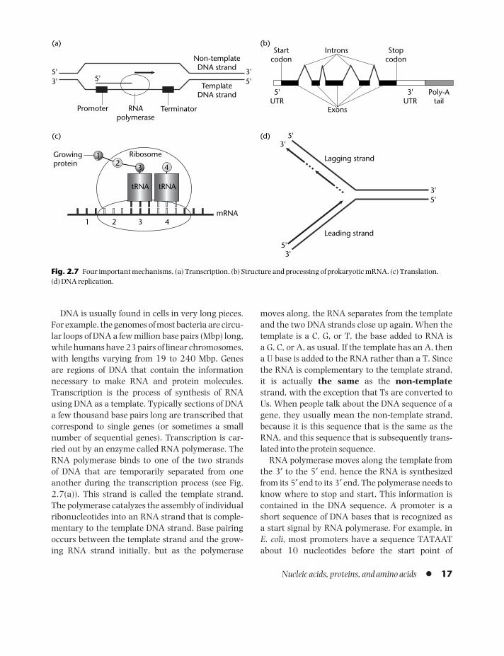
DNA is usually found in cells in very long pieces.For example, the genomes of most bacteria are circu-lar loops of DNA a few million base pairs (Mbp) long,while humans have 23 pairs of linear chromosomes,with lengths varying from 19 to 240 Mbp. Genes are regions of DNA that contain the informationnecessary to make RNA and protein molecules.Transcription is the process of synthesis of RNAusing DNA as a template. Typically sections of DNAa few thousand base pairs long are transcribed thatcorrespond to single genes (or sometimes a smallnumber of sequential genes). Transcription is car-ried out by an enzyme called RNA polymerase. TheRNA polymerase binds to one of the two strands of DNA that are temporarily separated from oneanother during the transcription process (see Fig.2.7(a)). This strand is called the template strand.The polymerase catalyzes the assembly of individualribonucleotides into an RNA strand that is comple-mentary to the template DNA strand. Base pairingoccurs between the template strand and the grow-ing RNA strand initially, but as the polymerase

moves along, the RNA separates from the templateand the two DNA strands close up again. When thetemplate is a C, G, or T, the base added to RNA is a G, C, or A, as usual. If the template has an A, then a U base is added to the RNA rather than a T. Sincethe RNA is complementary to the template strand, it is actually the same as the non-templatestrand, with the exception that Ts are converted toUs. When people talk about the DNA sequence of agene, they usually mean the non-template strand,because it is this sequence that is the same as theRNA, and this sequence that is subsequently trans-lated into the protein sequence.

RNA polymerase moves along the template fromthe 3′ to the 5′ end, hence the RNA is synthesizedfrom its 5′ end to its 3′ end. The polymerase needs toknow where to stop and start. This information iscontained in the DNA sequence. A promoter is ashort sequence of DNA bases that is recognized as a start signal by RNA polymerase. For example, in E. coli, most promoters have a sequence TATAATabout 10 nucleotides before the start point of

Nucleic acids, proteins, and amino acids l 17

Growingprotein

5'5'3'

3'5'

(a) (b)

(c) (d)

Promoter RNApolymerase

Terminator

Non-templateDNA strand

TemplateDNA strand

Startcodon

Introns

Exons

Stopcodon

5'UTR

3'UTR

Poly-Atail

5'3'

5'

5'

3'

3'

Lagging strand

Leading strand

1

1

2

2

3

3

4

4mRNA

tRNAtRNA

Ribosome

Fig. 2.7 Four important mechanisms. (a) Transcription. (b) Structure and processing of prokaryotic mRNA. (c) Translation. (d) DNA replication.

BAMC02 09/03/2009 16:43 Page 17

transcription and a sequence TTGACA about 35nucleotides before the start. However, these sequ-ences are not fixed, and there is considerable vari-ation between genes. Since promoters are relativelyshort and relatively variable in sequence, it is actually quite a hard problem to write a computerprogram to reliably locate them.

The stop signal, or terminator, for RNA poly-merase is often in the form of a specific sequence thathas the ability to form a hairpin loop structure in theRNA sequence. This structure delays the progres-sion of the polymerase along the template andcauses it to dissociate. We still have a lot more tolearn about these signals.

2.3.2 RNA processing

An RNA strand that is transcribed from a protein-coding region of DNA is called a messenger RNA(mRNA). The mRNA is used as a template for proteinsynthesis in the translation process discussed below.In prokaryotes, mRNAs consist of a central codingsequence that contains the information for makingthe protein and short untranslated regions (UTRs) at the 5′ and 3′ ends. The UTRs are parts of the sequ-ence that were transcribed but will not be translated.

In eukaryotes, the RNA transcript has a morecomplicated structure (Fig. 2.7(b)). When the RNAis newly synthesized, it is called a pre-mRNA. It mustbe processed in several ways before it becomes afunctional mRNA. At the 5′ end, a structure knownas a cap is added, which consists of a modified Gnucleotide and a protein complex called the cap-binding complex. At the 3′ end, a poly-A tail isadded, i.e., a string of roughly 200 A nucleotides.Proteins called poly-A binding proteins bind to thepoly-A tail. Many mRNAs have a rather short life-time (a few minutes) in the cell because they are bro-ken down by nuclease enzymes. These are proteinsthat break down RNA strands into individualnucleotides, either by chopping them in the middle(endonucleases), or by eating them up from the end one nucleotide at a time (exonucleases). Havingproteins associated with the mRNA, particularly atthe ends, slows down the nucleases. Variation in thetypes of binding protein on different mRNAs is an

important way of controlling mRNA lifetimes, andhence controlling the amount of protein synthesizedby limiting the number of times an mRNA can beused in translation.

Probably the most important type of RNA process-ing occurs in the middle of the pre-mRNA ratherthan at the ends. Eukaryotic gene sequences are broken up into alternating sections called exons and introns. Exons are the pieces of the sequencethat contain the information for protein coding.These pieces will be translated. Introns do not contain protein-coding information. The introns,indicated by the inverted Vs in Figure 2.7(b), are cut out of the pre-mRNA and are not present in themRNA after processing. When an intron is removed,the ends of the exons on either side of it are linkedtogether to form a continuous strand. This is knownas splicing.

Splicing is carried out by the spliceosome, a com-plex of several types of RNA and proteins boundtogether and acting as a molecular machine. Thespliceosome is able to recognize signals in the pre-mRNA sequence that tell it where the intron–exonboundaries are and hence which bits of the sequenceto remove. As with promoter sequences, the signals forthe splice sites are fairly short and somewhat variable,so that reliable identification of the intron–exon struc-ture of a gene is a difficult problem in bioinformatics.Nevertheless, the spliceosome manages to do it.

Introns that are spliced out by the spliceosome arecalled spliceosomal introns. This is the majority ofintrons in most organisms. In addition, there aresome interesting, but fairly rare, self-splicing introns,which have the ability to cut themselves out of anRNA strand without the action of the spliceosome.There are surprisingly large numbers of introns inmany eukaryotic genes – 10 or 20 in one gene is notuncommon. In contrast, most prokaryotic genes donot contain introns. It is still rather controversialwhere and when introns appeared, and what is theuse, if any, of having them.

In eukaryotes, the DNA is contained in the nucleus,and transcription and RNA processing occur in thenucleus. The mRNA is then transported out of the nucleus through pores in the nuclear membrane,and translation occurs in the cytoplasm.

18 l Chapter 2

BAMC02 09/03/2009 16:43 Page 18

2.3.3 The genetic code

We now need to consider the way information in theform of sequences of four types of base is turned intoinformation in the form of sequences of 20 types of amino acid. The mRNA sequence is read in groupsof three bases called codons. There are 43 = 64codons that can be made with four bases. Each ofthese codons codes for one type of amino acid, andsince 64 is greater than 20, most amino acids havemore than one codon that codes for them. The set of assignments of codons to amino acids is known as the genetic code, and is given in Table 2.1.

The table is divided into blocks that have the samebases in the first two positions. For example, codonsof the form UCN (where N is any of the four bases) allcode for Ser. There are many groups of four codonswhere all four code for the same amino acid and thebase at the third position does not make any differ-ence. There are several groups where there are twopairs of two amino acids in a block, e.g., CAY codes

for His and CAR codes for Gln (Y indicates a pyrimi-dine, C or U; and R indicates a purine, A or G). Thereare only two amino acids that have a single codon:UGG = Trp, and AUG = Met. Ile is unusual in havingthree codons, while Leu, Ser, and Arg all have sixcodons, consisting of a block of four and a block oftwo. There are three codons that act as stop signalsrather than coding for amino acids. These denotethe end of the coding region of a gene.

When the genetic code was first worked out in the1960s, it was thought to be universal, i.e., identicalin all species. Now we realize that it is extremelywidespread but not completely universal. The stan-dard code shown in Table 2.1 applies to almost allprokaryotic genomes (including both bacteria andarchaea) and to the nuclear genomes of almost alleukaryotes. In mitochondrial genomes, there areseveral different genetic codes, all differing from thestandard code in small respects (e.g., the reassign-ment of the stop codon UGA to Trp, or the reassign-ment of the Ile codon AUA to Met). There are also

Nucleic acids, proteins, and amino acids l 19

First position Second position Third position

U C A G

U Phe (F) Ser (S) Tyr (Y) Cys (C) UPhe (F) Ser (S) Tyr (Y) Cys (C) CLeu (L) Ser (S) STOP STOP ALeu (L) Ser (S) STOP Trp (W) G

C Leu (L) Pro (P) His (H) Arg (R) ULeu (L) Pro (P) His (H) Arg (R) CLeu (L) Pro (P) Gln (Q) Arg (R) ALeu (L) Pro (P) Gln (Q) Arg (R) G

A Ile (I) Thr (T) Asn (N) Ser (S) UIle (I) Thr (T) Asn (N) Ser (S) CIle (I) Thr (T) Lys (K) Arg (R) AMet (M) Thr (T) Lys (K) Arg (R) G

G Val (V) Ala (A) Asp (D) Gly (G) UVal (V) Ala (A) Asp (D) Gly (G) CVal (V) Ala (A) Glu (E) Gly (G) AVal (V) Ala (A) Glu (E) Gly (G) G

Table 2.1 The standard genetic code. This is used in most prokaryotic genomes and in the nuclear genomes of most eukaryotes.

BAMC02 09/03/2009 16:43 Page 19

some changes in the nuclear genome codes for specificgroups of organisms, such as the ciliates (a group ofunicellular eukaryotes including Tetrahymena andParamecium), and Mycoplasma bacteria use a slightlydifferent code from most bacteria. These changes areall quite small, and presumably they occurred at arelatively late stage in evolution. The main messageis that the code is shared between all three domainsof life (archaea, bacteria, and eukaryotes) and hencemust have evolved before the divergence of thesegroups. Thus the last universal common ancestor ofall current life must have used this genetic code.

Here we will pause to write a letter of complaint tothe BBC. When the release of the human genomesequence was announced in 2001, there were manycurrent affairs broadcasters who commented onhow exciting it is that we now know the complete“human genetic code”. We have known the geneticcode for 40 years! What is new is that we now havethe complete genome sequence. Please do not confuse the genetic code with the genome. We nowhave the complete book, whereas 40 years ago weonly knew the words in which the book is written. It will probably take us another 40 years to under-stand what the book means.

2.3.4 Translation and protein synthesis

Translation is the process of synthesis of a pro-tein sequence using mRNA as a template. A keymolecule in the process is transfer RNA (tRNA). The structure of tRNA was already shown in Fig. 2.4 and Plate 2.1(a). The three bases in the middle of the central hairpin loop in the cloverleaf are calledthe anticodon. The sequence shown in Fig. 2.4 is a tRNA-Ala, i.e., a tRNA for the amino acid alanine.The anticodon of this molecule is UGC (reading from5′ to 3′) in the tRNA. This can form complementarybase pairs with the codon sequence GCA (readingfrom 5′ to 3′ in the mRNA) like this:

| |C – G – U tRNA

–G – C – A– mRNA

Note that GCA is an alanine codon in the geneticcode. Organisms possess sets of tRNAs capable of

base pairing with all 61 codons that denote aminoacids. These tRNAs have different anticodons, andare also different from one another in many otherparts of the sequence, but they all have the samecloverleaf secondary structure.

It is not true, however, that there is one tRNA thatexactly matches every codon. Many tRNAs can pairwith more than one codon due to the flexibility of thepairing rules that occurs at the third position in thecodon – this is known as wobble. For example, mostbacteria have two types of tRNA-Ala. One type, withanticodon UGC, decodes the codons GCA and GCG,while the other type, with anticodon GGC, decodesthe codons GCU and GCC. The actual number oftRNAs varies considerably between organisms. Forexample, the E. coli K12 genome has 86 tRNA genes,of which three have UGC and two have GGC anti-codons. In contrast Rickettsia prowazeckii, anothermember of the proteobacteria group, has a muchsmaller genome with only 32 tRNAs, and only oneof each type of tRNA-Ala. These figures are all takenfrom the genomic tRNA database (Lowe and Eddy,1997). In eukaryotes, the wobble rules tend to beless flexible, so that a greater number of distincttRNA types are required. Also the total number oftRNA genes can be much larger, due to the presenceof duplicate copies. Thus, in humans, there areabout 496 tRNAs in total, and for tRNA-Ala thereare 10 with UGC anticodon, five with CGC, and 25with AGC. In contrast, in most mitochondrialgenomes, there are only 22 tRNAs capable of decod-ing the complete set of codons. In this case, when-ever there is a box of four codons, only one tRNA isrequired. Pairing at the third position is extremelyflexible (sometimes known as hyperwobble). For ex-ample the tRNA-Ala, with anticodon UGC, decodesall codons of the form GCN.

Transfer RNA acts as an adaptor molecule. Theanticodon end connects to the mRNA, and the otherend connects to the growing protein chain. EachtRNA has an associated enzyme, known as anamino acyl-tRNA synthetase, whose function is toattach an amino acid of the correct type to the 3′ endof the tRNA. The enzyme and the tRNA recognizeone another specifically, due to their particular shapeand intermolecular interactions. The interaction

20 l Chapter 2

BAMC02 09/03/2009 16:43 Page 20

between glutaminyl-tRNA synthetase and tRNA-glutamine is shown in Plate 2.1(a).

Protein synthesis is carried out by another mole-cular machine called a ribosome. The ribosome iscomposed of a large and a small subunit (repres-ented by the two large ellipses in the cartoon in Fig. 2.7(c)). In bacteria, the small subunit containsthe small subunit ribosomal RNA (SSU rRNA),which is typically 1500 nucleotides long, togetherwith about 20 ribosomal proteins. The large subunit contains large subunit ribosomal RNA (LSU rRNA),which is typically 3000 nucleotides long, togetherwith about 30 proteins and another smaller ribo-somal RNA known as 5S rRNA. The ribosomes of eukaryotes are larger – the two major rRNAmolecules are significantly longer and the number ofproteins in each subunit is greater.

Figure 2.7(c) illustrates the mechanism of proteinsynthesis. The ribosome binds to the mRNA andmoves along it one codon at a time. tRNAs, chargedwith their appropriate amino acid, are able to bind tothe mRNA at a site inside the ribosome. The aminoacid is then removed from the tRNA and attached tothe end of a growing protein chain. The old tRNA thenleaves and can be recharged with another moleculeof the same type of amino acid and used again. ThetRNA corresponding to the next codon then binds tothe mRNA and the ribosome moves along one codon.

Just as with transcription, translation also requiressignals to tell it where to start and stop. We alreadymentioned stop codons. These are codons that do nothave a matching tRNA. When the ribosome reachesa stop codon, a protein known as a release factorenters the appropriate site in the ribosome instead ofa tRNA. The release factor triggers the release of thecompleted protein from the ribosome.

There is also a specific start codon, AUG, whichcodes for methionine. The ribosome begins proteinsynthesis at the first AUG codon it finds, which willbe slightly downstream of the place where it initiallybinds to the mRNA. In bacteria, mRNAs contain a conserved sequence of about eight nucleotides,called the Shine–Dalgarno sequence, close to their5′ end. This sequence is complementary to part ofSSU rRNA in the small subunit of the ribosome. Thisinteraction triggers the binding of the ribosome to

the mRNA. The first tRNA involved is known as anfMet initiator tRNA. This is a special type of tRNA-Met, where a formyl group has been added to themethionine on the charged tRNA. The fMet is onlyused when an AUG is a start codon. Other AUGcodons occurring in the middle of a gene sequencelead to the usual form of Met being added to the protein sequence.

In the last few years, we have been able to obtainthree-dimensional crystal structures of the ribosome(e.g., Yusupov et al. 2001), and we are getting closerto understanding the mechanism by which the ribo-some actually works. The ribosome is acting as a catalyst for the process of peptide bond formation.“Ribozyme” is the term used for a catalytic RNAmolecule, by analogy with “enzyme”, which is a cata-lytic protein. It had previously been thought thatrRNA was simply a scaffold onto which the ribo-somal proteins attached themselves, and that it wasthe catalytic action of the proteins that achieved pro-tein synthesis. Recent experiments are making itclear that rRNA plays an essential role in the cata-lysis, and hence that rRNA is a type of ribozyme.

2.3.5 Closing the loop: DNA replication

As stated above, the central dogma is the principlethat information is stored in DNA, is transferredfrom DNA to RNA, and then from RNA to proteins.We have now briefly explained the mechanisms bywhich this occurs. In order to close the loop in ourexplanation of the synthesis of nucleic acids and pro-teins, we still need to explain how DNA is formed.

DNA needs to be replicated every time a celldivides. In a multicellular organism, each cell con-tains a full copy of the genome of the organism towhich it belongs (with the exception of certain cellswithout nuclei, such as red blood cells). The DNA is needed in every cell in order that transcription and translation can proceed in those cells. DNA re-plication is also essential for reproduction, becauseDNA contains the genetic information that ensuresheredity.

DNA replication is semi-conservative. This meansthat the original double strand is replicated to givetwo double strands, each of which contains one of

Nucleic acids, proteins, and amino acids l 21

BAMC02 09/03/2009 16:43 Page 21

the original strands and one newly synthesizedstrand that is complementary to it. Clearly, bothstrands of DNA contain the full information neces-sary to recreate the other strand. The key processesof DNA replication occur at a replication fork (Fig.2.7(d)). At this point, the two old strands are separ-ated from one another and the new strands are syn-thesized. The main enzyme that does this job is DNApolymerase III. This enzyme catalyzes the addition ofnucleotides to the 3′ ends of the growing strands (atthe heads of the arrows in Fig. 2.7(d)). The newstrand is therefore synthesized in the 5′ to 3′ direc-tion (as with mRNA synthesis during transcription).On one strand, called the leading strand, synthesis is possible in a continuous unbroken fashion. How-ever, on the lagging strand on the opposite side, con-tinuous synthesis is not possible and it is necessaryto initiate synthesis independently many times. Thenew strand is therefore formed in pieces, which areknown as Okazaki fragments.

DNA polymerase III is able to carry out the additionof new nucleotides to a strand but it cannot initiate anew strand. This is in contrast to RNA polymerase,which is able to perform both initiation and addition.DNA polymerase therefore needs a short sequence,called a primer, from which to begin. Primers areshort sequences of RNA (indicated by dotted lines inFig. 2.7(d)) that are synthesized by a form of RNApolymerase called primase. The processes of DNAsynthesis initiated by primers has been harnessed tobecome an important laboratory tool, the poly-merase chain reaction or PCR (see Box 2.1).

Once the fragments on the lagging strand havebeen synthesized, it is necessary to connect themtogether. This is done by two more enzymes. DNApolymerase I removes the RNA nucleotides of theprimers and replaces them with DNA nucleotides.DNA ligase makes the final connection between thefragments. Both DNA polymerase I and III have theability to excise nucleotides from the 3′ end if they donot match the template strand. This process of errorcorrection is called proof-reading. This means thatthe fidelity of replication of DNA polymerase isincreased by several orders of magnitude withrespect to RNA polymerases. Errors in DNA replica-tion cause heritable point mutations, whereas errors

in RNA replication merely lead to mistakes in a sin-gle short-lived mRNA. Hence accurate DNA replica-tion is very important.

We called this section “closing the loop” because,in the order that we presented things here, DNAreplication is the last link in the cycle of mechan-isms for synthesis of the major biological macro-molecules. There is, however, a more fundamentalsense in which this whole process is a loop. Clearlyproteins cannot be synthesized without DNA be-cause proteins do not store genetic information.DNA can store this information, but it cannot carryout the catalytic roles necessary for metabolism in a cell, and it cannot replicate itself without the aid of proteins. There is thus a chicken and egg situ-ation: “Which came first, DNA or proteins?” Manypeople now believe that RNA preceded both DNAand proteins, and that there was a period in theEarth’s history when RNA played both the geneticand catalytic roles. This is a tempting hypothesis,because several types of catalytic RNA are known(both naturally occurring and artificially synthes-ized sequences), and because many viruses use RNA as their genetic material today. As with all con-jectures related to the origin of life and very earlyevolution, however, it is difficult to prove that anRNA world once existed.

2.4 PHYSICO-CHEMICAL PROPERTIESOF THE AMINO ACIDS AND THEIRIMPORTANCE IN PROTEIN FOLDING

As we mentioned in Section 1.1, we have many pro-tein sequences for which experimentally determinedthree-dimensional structures are unavailable. Along-standing goal of bioinformatics has been to pre-dict protein structure from sequence. Some methodsfor doing this will be discussed in Chapter 10 on pat-tern recognition. In this section, we will introducesome of the physico-chemical properties that arethought to be important for determining the way aprotein folds.

One property that obviously matters for aminoacids is size. Proteins are quite compact in structure,and the different residues pack together in a way

22 l Chapter 2

BAMC02 09/03/2009 16:43 Page 22

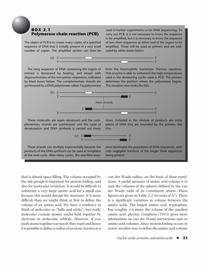
that is almost space filling. The volume occupied bythe side groups is important for protein folding, andalso for molecular evolution. It would be difficult tosubstitute a very large amino acid for a small onebecause this would disrupt the structure. It is moredifficult than we might think at first to define the volume of an amino acid. We have a tendency tothink of molecules as “balls and sticks”, but reallymolecules contain atomic nuclei held together byelectrons in molecular orbitals. However, if youpush atoms together too much, they repel and henceit is possible to define a radius of an atom, known as a

van der Waals radius, on the basis of these repul-sions. A useful measure of amino acid volume is tosum the volumes of the spheres defined by the vander Waals radii of its constituent atoms. Thesefigures are given in Table 2.2 (in units of Å3). Thereis a significant variation in volume between theamino acids. The largest amino acid, tryptophan,has roughly 3.4 times the volume of the smallestamino acid, glycine. Creighton (1993) gives moreinformation on van der Waals interactions and onamino acid volumes. Since protein folding occurs inwater, another way to define the amino acid volume

Nucleic acids, proteins, and amino acids l 23

BOX 2.1Polymerase chain reaction (PCR)

The object of PCR is to create many copies of a specifiedsequence of DNA that is initially present in a very smallnumber of copies. The amplified section can then be

used in further experiments or for DNA sequencing. Tocarry out PCR, it is not necessary to know the sequenceto be amplified, but it is necessary to know the sequenceof two short sequences at either end of the region to beamplified. These will be used as primers and are indi-cated by white boxes below.

5'3'

3'5'

5'3'

3'5'

(b)

New strands

5'3'

3'5'

(c)

5'3'

3'5'

(a)

The long sequence of DNA containing the region ofinterest is denatured by heating, and mixed witholigonucleotides of the two primer sequences, indicatedby black boxes below. The complementary strands aresynthesized by a DNA polymerase called Taq polymerase

from the thermophilic bacterium Thermus aquaticus.This enzyme is able to withstand the high temperaturesused in the denaturing cycles used in PCR. The primersdetermine the position where the polymerase begins.The situation now looks like this:

These molecules are again denatured and the com-plementary strands are synthesized, and the cycle ofdenaturation and DNA synthesis is carried out many

times. Included in the mixture of products are somepieces of DNA that are bounded by the primers, like this:

These strands can multiply exponentially because theproducts of the DNA synthesis can be used as templatesat the next cycle. After many cycles, the specified sequ-

ence dominates the population of DNA sequences, withonly negligible fractions of the longer DNA sequencesbeing present.

BAMC02 09/03/2009 16:43 Page 23

is to consider the increase in volume of a solutionwhen an amino acid is dissolved in it. This is knownas the partial volume. Partial volumes are closelycorrelated with the volumes calculated from the van der Waals radii, and we do not show them in the table.

Zimmerman, Eliezer, and Simha (1968) presenteddata on several amino acid properties that are relev-ant in the context of protein folding. Rather thansimply considering the volume, they defined the“bulkiness” of an amino acid as the ratio of the sidechain volume to its length, which provides a meas-ure of the average cross-sectional area of the side

chain. These figures are shown in Table 2.2 (in Å2).Zimmerman, Eliezer, and Simha (1968) also intro-duced a measure of the polarity of the amino acids.They calculated the electrostatic force of the aminoacid acting on its surroundings at a distance of 10 Å.This is composed of the force from the electric charge(for the amino acids that have a charged side group)plus the force from the dipole moment (due to thenon-uniformity of electronic charge across the aminoacid). The total force (in units scaled for convenience)was used as a polarity index, and this is shown inTable 2.2. The electrostatic charge term, where it ex-ists, is much larger than the dipole term. Hence, this

24 l Chapter 2

Vol. Bulk. Polarity pI Hyd.1 Hyd.2 Surface Fract. area area

Alanine Ala A 67 11.50 0.00 6.00 1.8 1.6 113 0.74Arginine Arg R 148 14.28 52.00 10.76 −4.5 −12.3 241 0.64Asparagine Asn N 96 12.28 3.38 5.41 −3.5 −4.8 158 0.63Aspartic acid Asp D 91 11.68 49.70 2.77 −3.5 −9.2 151 0.62Cysteine Cys C 86 13.46 1.48 5.05 2.5 2.0 140 0.91Glutamine Gln Q 114 14.45 3.53 5.65 −3.5 −4.1 189 0.62Glutamic acid Glu E 109 13.57 49.90 3.22 −3.5 −8.2 183 0.62Glycine Gly G 48 3.40 0.00 5.97 −0.4 1.0 85 0.72Histidine His H 118 13.69 51.60 7.59 −3.2 −3.0 194 0.78Isoleucine Ile I 124 21.40 0.13 6.02 4.5 3.1 182 0.88Leucine Leu L 124 21.40 0.13 5.98 3.8 2.8 180 0.85Lysine Lys K 135 15.71 49.50 9.74 −3.9 −8.8 211 0.52Methionine Met M 124 16.25 1.43 5.74 1.9 3.4 204 0.85Phenylalanine Phe F 135 19.80 0.35 5.48 2.8 3.7 218 0.88Proline Pro P 90 17.43 1.58 6.30 −1.6 −0.2 143 0.64Serine Ser S 73 9.47 1.67 5.68 −0.8 0.6 122 0.66Threonine Thr T 93 15.77 1.66 5.66 −0.7 1.2 146 0.70Tryptophan Trp W 163 21.67 2.10 5.89 −0.9 1.9 259 0.85Tyrosine Tyr Y 141 18.03 1.61 5.66 −1.3 −0.7 229 0.76Valine Val V 105 21.57 0.13 5.96 4.2 2.6 160 0.86Mean 109 15.35 13.59 6.03 −0.5 −1.4 175 0.74Std. dev. 28 4.53 21.36 1.72 2.9 4.8 44 0.11

Vol., volume calculated from van der Waals radii (Creighton 1993); Bulk., bulkiness index (Zimmerman, Eliezer, and Simha 1968); Polarity, polarity index (Zimmerman, Eliezer, and Simha 1968); pI, pH of the isoelectric point (Zimmerman, Eliezer, and Simha 1968); Hyd.1, hydrophobicity scale (Kyte and Doolittle 1982); Hyd.2,hydrophobicity scale (Engelman, Steitz, and Goldman 1986); Surface area, surface area accessible to water in unfolded peptide (Miller et al. 1987); Fract. area, fraction of accessible area lost when a protein folds (Rose et al. 1985).

Table 2.2 Physico-chemical properties of the amino acids.

BAMC02 09/03/2009 16:43 Page 24

measure clearly distinguishes between the chargedand uncharged amino acids.

The polarity index does not distinguish betweenthe positively and negatively charged amino acids,however, since both have high polarity. A quantitythat does this is the pI, which is defined as the pH ofthe isoelectric point of the amino acid. Acidic aminoacids (Asp and Glu) have pI in the range 2–3. Thismeans that these amino acids would be negativelycharged at neutral pH due to ionization of the COOHgroup to COO−. We need to put them in an acid solu-tion in order to shift the equilibrium and balance thischarge. The basic amino acids (Arg, Lys, and His)have pI greater than 7. All the others usually haveuncharged side chains in real proteins. They have pIin the range 5–6. Thus, pI is a useful measure ofacidity of amino acids that distinguishes clearly be-tween positive, negative, and uncharged side chains.

A key factor in protein folding is the “hydrophobiceffect”, which arises as a result of the unusual char-acteristics of water as a solvent. Liquid water hasquite a lot of structure due to the formation of chainsand networks of molecules interacting via hydrogenbonds. When other molecules are dissolved in water,the hydrogen-bonded structure is disrupted. Polaramino acid residues are also able to form hydrogenbonds with water. They therefore disrupt the struc-ture less than non-polar amino acids that are unableto form hydrogen bonds. We say that the non-polaramino acids are hydrophobic, because they do not“want” to be in contact with water, whereas thepolar amino acids are hydrophilic, because they“like” water. It is generally observed that hydro-phobic residues in a protein are in the interior of the structure and are not in contact with water,whereas hydrophilic residues are on the surface andare in contact with water. In this way the free energyof the folded molecule is minimized.

Kyte and Doolittle (1982) defined a hydrophobicity(or hydropathy) scale that is an estimate of the differ-ence in free energy (in kcal/mol) of the amino acidwhen it is buried in the hydrophobic environment ofthe interior of a protein and when it is in solution inwater. Positive values on the scale mean that theresidue is hydrophobic: it costs free energy to takethe residue out of the protein and put it in water.

Another version of the hydrophobicity scale wasdeveloped by Engelman, Steitz, and Goldman (1986),who were particularly interested in membrane pro-teins. The interior of a lipid bilayer is hydrophobic,because it mostly consists of the hydrocarbon tails ofthe lipids. They estimated the free energy cost forremoval of an amino acid from the bilayer to water.These two scales are similar but not identical; there-fore both scales are shown in the table.

Another property that is thought to be relevantfor protein folding is the surface area of the aminoacid that is exposed (accessible) to water in anunfolded peptide chain and that becomes buriedwhen the chain folds. Table 2.2 shows the accessiblesurface areas of the residues when they occur in aGly–X–Gly tripeptide (Miller et al. 1987, Creighton1993). Rose et al. (1985) calculated the averagefraction of the accessible surface area that is buriedin the interior in a set of known crystal structures.They showed that hydrophobic residues have alarger fraction of the surface area buried, which sup-ports the argument that the “hydrophobic effect” isimportant in determining protein structure.

2.5 VISUALIZATION OF AMINO ACID PROPERTIES USING PRINCIPALCOMPONENT ANALYSIS

So far, this chapter has summarized some of the fun-damental aspects of molecular biology that we thinkevery bioinformatician should know. In the rest of thechapter, we want to introduce some simple methodsfor data analysis that are useful in bioinformatics.We will use the data on amino acid properties.

Table 2.2 shows eight properties of each aminoacid (and we could easily have included severalmore columns using data from additional sources).It would be useful to plot some kind of diagram thatlets us visualize the information in this table. It isstraightforward to take any two of the propertiesand use these as the coordinates for the points in a two-dimensional graph. Figure 2.8 shows a plot of volume against pI. This clearly shows the acidicamino acids at low pI, the basic amino acids at highpI, and all the rest in the middle. It also shows the

Nucleic acids, proteins, and amino acids l 25

BAMC02 09/03/2009 16:43 Page 25

large spread of the middle group along the volumeaxis. However, the figure does not distinguishbetween the hydrophilic and hydrophobic aminoacids in the middle group: N and Q appear very closeto M and V, for example. We could separate these byusing one of the hydrophobicity scales on the axisinstead of pI, but then the acidic and basic groupswould appear close together because both arehydrophilic (negative on the hydrophobicity scale).What we need is a way of combining the informa-tion from all eight properties into a two-dimensionalgraph. This can be done with principal componentanalysis (PCA).

In general with PCA, we begin with the data in theform of an N × P matrix, like Table 2.2. The numberof rows, N, is the number of objects in our data set (inthis case N = 20 amino acids), and the number ofcolumns, P, is the number of properties of thoseobjects (in this case P = 8). Each row in the datamatrix can be thought of as the coordinates of apoint in P-dimensional space. The whole data set is acloud of these points. The PCA method transformsthis cloud of points first by scaling them and shiftingthem to the origin, and then by rotating them insuch a way that the points are spread out as much aspossible, and the structure in the data is made easierto see.

Let the original data matrix be Xij(i.e., Xij is thevalue of the jth property of object i). The mean andstandard deviation of the properties are

and

The mean and standard deviation are listed at thefoot of Table 2.2. Since the properties all have differ-ent scales and different mean values, the first step ofPCA is to define scaled data values by

zij = (Xij − µj)/σj

The zij matrix measures the deviation of the valuesfrom the mean values for each property. By defin-ition, the mean value of each column in the zij matrixis 0 and the standard deviation is 1. Scaling the datain this way means that all the input properties areplaced on an equal footing, and all the properties willcontribute equally to the data analysis.

We now choose a set of vectors vj = (vj1, vj2, vj3,. . . vjP) that define the directions of the principal

σ µj ij jiN

X ( )/

= −⎛

⎝⎜⎞

⎠⎟∑1 2

1 2

µ j ijiN

X = ∑1

26 l Chapter 2

100

120

140

160

40

60

80

180

2 4 6pI

8 10 12

Volu

me

(Å3 )

D

E

CT P

AS

G

HM

LI

Q

NV

W

FY

K

R

Fig. 2.8 Plot of amino acid volumeagainst pI – two properties thought tobe important in protein folding.

BAMC02 09/03/2009 16:43 Page 26

components. These vectors are of unit length, i.e.,

for each vector, and they are all orthogonal

to one another, i.e., when i and j are not

equal. Each vector represents a new coordinate axisthat is a linear combination of the old coordinates.The positions of the points in the new coordinate sys-tem are given by

The new y coordinate system is a rotation of the zcoordinate system – see Fig. 2.9.

There are still P coordinates, so we can only usetwo of them if we plot a two-dimensional graph.However, we can define the y coordinates so that asmuch of the variation between the points as possibleis visible in the first few coordinates. We thereforechoose the v1k values so that the variance of thepoints along the first principal component axis,

is as large as possible. (Note that the

means of the y’s are all zero because the means of thez’s were zero.) We then choose the v2k for the second

component by maximizing the variance

with the constraint that the second axis is orthogonal

to the first, i.e., If we wish, we can

define further components by maximizing the vari-

v vk kk

1 2 0∑ = .

12

2

Nyi

i

,∑

112

Nyi

i

∑

y v zij jk ikk

= ∑

v vik jkk∑ = ,0

v jkk

2 1 =∑ance with the constraint that each component isorthogonal to the previous ones. Calculation of thevjk is discussed in more detail in Box 2.2.

The results of PCA for the amino acid data in Table 2.2 are shown in Fig. 2.10. The first two principal component vectors are shown in thematrix on p. 28. For component 1, the largest contributions in the vector are the negative con-tributions from the hydrophobicity scales. Thushydrophobic amino acids appear on the left side and hydrophilic ones on the right. For component 2,the largest contributions are positive ones from volume, bulkiness, and surface area. Thus largeamino acids appear near the top of the figure andsmall ones near the bottom. However, all the pro-perties contribute to some extent to each of the com-ponents; therefore, the resulting figure is not thesame as we would have got by simply plottinghydrophobicity against volume.

Figure 2.10 illustrates several points about thedata that seem intuitive. There is a cluster ofmedium-sized hydrophobic residues, I, L, V, M, andF. The two acids, D and E, are close, and so are thetwo amides, Q and N. Two of the basic residues, Rand K, are very close, and H is fairly close to these.The two largest residues, W and Y, are quite close toone another. The PCA diagram manages to do afairly good job at illustrating all these similarities atthe same time.

The PCA calculation in this section was doneusing the program pca.c by F. Murtagh (http://astro.u-strasbg.fr/~fmurtagh/mda-sw/).

Nucleic acids, proteins, and amino acids l 27

X2

X1

X3

(a) z2

z1

z3

(b) y2

y1

y3

(c)

Fig. 2.9 Schematic illustration of principal component analysis. (a) Original data. (b) Scaled and centered on the origin. (c) Rotated onto principal components.

BAMC02 09/03/2009 16:43 Page 27

2.6 CLUSTERING AMINO ACIDSACCORDING TO THEIR PROPERTIES

2.6.1 Handmade clusters

When we look at a figure like 2.10, it is natural to tryto group the points into “clusters” of similar objects.We already remarked above that I, L, V, M, and Flook like a cluster. So, where would you put clusters?Before going any further, make a few photocopies ofFig. 2.10. Now take one of the copies and draw ringsaround the groups of points that you think should beclustered. You can decide how many clusters youthink there should be – somewhere between fourand seven is probably about right. You can alsodecide how big the clusters should be – you can putlots of points together in one cluster if you like, oryou can leave single points on their own in a clusterof size one. OK, go ahead!

When we presented the chemical structures of theamino acids in Fig. 2.6, we chose four groups:

Neutral, nonpolar W, F, G, A, V, I, L, M, PNeutral, polar Y, S, T, N, Q, CAcidic D, EBasic K, R, H

This is one possible clustering. We chose these fourclusters because this is the way the amino acids arepresented in most molecular biology textbooks. Trydrawing rings round these four clusters on anothercopy of Fig. 2.10. The acidic and basic groups workquite well. The neutral polar group forms a ratherspread-out cluster in the middle of the figure, butunfortunately it has P in the middle of it. The nonpo-lar group can hardly be called a cluster, as it takes upabout half the diagram, and contains points that arevery far from one another, like G and W. You prob-ably think that you did a better job when you madeup your own clusters a few minutes ago.

We now want to consider ways of clustering datathat are more systematic than drawing rings on paper.

28 l Chapter 2

0.8

–0.8

–1.0

0

0.2

–0.2

0.4

–0.4

0.6

–0.6

–0.2–0.4–0.6 0.2 0.40First component

0.6 0.8

Seco

nd c

omp

onen

t I LM

F

V

C

W

Y

A

T P

S

G

Q

N

H

E

D

K

R

Fig. 2.10 Plot of the amino acids onthe first two components of theprincipal component analysis.

Vol Bulk. Pol. pI Hyd.1 Hyd.2 S.A. Fr.A.Comp. 1 (0.06, −0.22, 0.44, 0.19, −0.49, −0.51, 0.10, −0.45)Comp. 2 (0.58, 0.48, 0.10, 0.25, 0.03, −0.03, 0.56, 0.17)

BAMC02 09/03/2009 16:43 Page 28

Nucleic acids, proteins, and amino acids l 29

BOX 2.2Principal component analysis in more detail

From the N × P data matrix, we can define a P × P matrix of correlation coefficients, Cjk, between the properties:

The coefficients are always in the range −1 to 1. If Cjk > 0, the two properties are positively correlated, i.e., they bothtend to be large at the same time and small at the same time. If Cjk < 0, the properties are negatively correlated, i.e.,one tends to be large when the other is small. The correlation matrix for the amino acid data looks like this.

The matrix is symmetric (Cjk = Ckj) and all the diagonal elements are 1.00 by definition. The values illustrate fea-tures of the data that are not easy to see in the original matrix. For example, volume has a strong positive correlationwith surface area and bulkiness, and a fairly weak correlation with the other properties. The two hydro-phobicity scales have strong positive correlation with each other and also with the fractional area property, but theyhave a significant negative correlation with the polarity scale.

It can be shown that the vectors vj that define the principal component axes are the eigenvectors of the correlationmatrix, i.e., they satisfy the equation:

= lnvnk

where the ln are constants called eigenvalues. The first principal component (PC) vector is the eigenvector with thelargest eigenvalue. Subsequent PCs can be listed in order of decreasing size of eigenvalue. The first two eigenvaluesin this case are l1 = 3.57 and l2 = 2.81.

The variance along the nth PC axis is equal to the corresponding eigenvalue:

We know that the variance of each of the z coordinates is 1, hence the total variance of all the coordinates is P. Whenwe change the coordinates to the principal components, we just rotate the points in space, so the total variance in the PC space is still P. The fraction of the total variance represented by the first two PCs is therefore (l1 + l2)/P, which in our case is (3.57 + 2.81)/8 = 0.797. This is why it is useful to look at the data on the PC plot (asin Fig. 2.10). Roughly 80% of the variation in the positioning of the points in the original coordinates can be seenwith just two PCs. When points appear close in the two-dimensional plot of the first two PCs, they really are close inthe eight-dimensional space, because the remaining six dimensions that we can’t see do not contribute much to thedistance between the points. This means that if we spot patterns in the data in the PC plot, such as clusters of closelyspaced points, then these are likely to give a true impression of the patterns in the full data.

1 12 2

Ny

Nv z v z v C v vin

inj ij nk ik

kjinj jk nk

kjn nk

kn∑ ∑∑∑ ∑∑ ∑= = = = l l

v Cnj jkj

∑

CN

X XN

z zjkj K

ij ji

ik k ij iki

( )( ) = − − =∑ ∑1 1s s

m m

Vol Bulk. Pol. pI Hyd.1 Hyd.2 S.A. Fr.A.Vol. 1.00 0.73 0.24 0.37 −0.08 −0.16 0.99 0.18Bulk. 0.73 1.00 −0.20 0.08 0.44 0.32 0.64 0.49Pol. 0.24 −0.20 1.00 0.27 −0.69 −0.85 0.29 −0.53pI 0.37 0.08 0.27 1.00 −0.20 −0.27 0.36 −0.18Hyd.1 −0.08 0.44 −0.67 −0.20 1.00 0.85 −0.18 0.84Hyd.2 −0.16 0.32 −0.85 −0.27 0.85 1.00 −0.23 0.79S.A. 0.99 0.64 0.29 0.36 −0.18 −0.23 1.00 0.12Fr.A. 0.18 0.49 −0.53 −0.18 0.84 0.79 0.12 1.00

BAMC02 09/03/2009 16:43 Page 29

In fact, there is a huge number of different clusteringmethods. This testifies to the fact that there are a lotof different people from a lot of different disciplineswho find clustering useful for describing the patternsin their data. Unfortunately, it also means that thereis not one single clustering method that everyoneagrees is best. Different methods will give differentanswers when applied to the same data; therefore,there has to be some degree of subjectivity in decid-ing which method to use for any particular data set.

In the context of the amino acids, clusteringaccording to physico-chemical properties is actu-ally quite helpful when we come to do proteinsequence alignments. We usually want to alignresidues with similar properties with one another,even if the residues are not identical. There are sev-eral sequence alignment editors that ascribe colorsto residues, assigning the same color to clusters of similar amino acids. In well-aligned parts of proteinsequences, we often find that all the residues in a column have the same color. The coloring schemecan thus help with constructing alignments andspotting important conserved motifs. When we lookat protein sequence evolution (Chapter 4) it turnsout that substitutions are more frequent betweenamino acids with similar properties. So, clusteringaccording to properties is also relevant for evolution.In the broader context, however, clustering algo-rithms are very general and can be used for almostany type of data. In this book, they will come upagain in two places: in Chapter 8 we discuss distancematrix methods for molecular phylogenetics, whichare a form of hierarchical clustering; and in Chapter13 we discuss applications of clustering algorithmson microarray data. It is therefore worth spendingsome time on these methods now, even if you aregetting a bit bored with amino acid properties.

2.6.2 Hierarchical clustering methods

In a hierarchical clustering method, we need tochoose a measure of similarity between the datapoints, then we need to choose a rule for measuringthe similarity of clusters.

We will use the scaled coordinates z as in the pre-vious section. There is a vector zi from the origin to

each point i in the data set (see Fig. 2.11). The lengthof the vector is:

We want to measure how similar the vectors are fortwo points i and j. A simple way to do this is to use thecosine of the angle θij between the vectors. If the twovectors are pointing in almost the same direction, θijwill be small and cos θij will be close to 1. Vectorswith no correlation will have θij close to 90° and cos θij close to 0. Vectors with negative correlationwill have θij > 90° and cos θij < 0.

From standard geometry,

Another possible similarity measure is the correla-tion coefficient between the z vectors:

where mi and si are the mean and standard deviationof the elements in the ith row (see also Box 2.2, wherewe define the correlation between the columns). Rij is in the range −1 to 1.

In what follows, we shall assume that we havecalculated an N × N matrix of similarities betweenthe data points that could be cos θij or Rij, or anyother measure of similarity that appears appropriatefor the data in question. We will call the similarity

RPs s

z m z miji j

ik i jk jk

( )( )= − −∑1

cos

| || |θij

ik jkk

i j

z z

=∑

z z

| | /

z zi ikk

=⎛

⎝⎜⎞

⎠⎟∑ 2

1 2

30 l Chapter 2

z2

i

j

z1

z3

dij

θij

Fig. 2.11 Illustration of the data points as vectors inmultidimensional space.

BAMC02 09/03/2009 16:43 Page 30

matrix Sij from now on, to emphasize that themethod is general and works the same way, which-ever measure we use for similarity.

During the process of hierarchical clustering,points are combined into clusters, and small clustersare combined to give progressively larger clusters.To decide in what order these clusters will be con-nected, we will need a definition of similarity betweenclusters. Suppose we already have two clusters Aand B. We want to define the similarity SAB of theseclusters. There are (at least) three ways of doing this:• Group average. SAB = the mean of the similaritiesSij between the individual data points, averaged overall pairs of points, where i is in cluster A and j is incluster B.• Single-link rule. SAB = maximum similarity Sij forany i in A and j in B.• Complete-link rule. SAB = minimum similarity Sijfor any i in A and j in B.The reasons for the terms “single link” and “com-plete link” will be made more clear in Section 2.6.3.

An algorithm is a computational recipe thatspecifies how to solve a problem. Algorithms comeup throughout this book, and we will discuss somegeneral points about algorithms in Chapter 6. Forthe moment, we will present a very simple algorithmfor hierarchical clustering. This works in the sameway, whatever the definitions of similarity betweendata points and between clusters. We begin witheach point in a separate cluster of its own.1 Join the two clusters with the highest similarity toform a single larger cluster.2 Recalculate similarities between all the clustersusing one of the three definitions above.3 Repeat steps 1 and 2 until all points have beenconnected to a single cluster.This procedure is called “hierarchical” because it gen-erates a set of clusters within clusters within clusters.For this reason, the results of a hierarchical clusteringprocedure can be represented as a tree. Each branch-ing point on the tree is a point where two smallerclusters were joined to form a larger one. Readingbackwards from the twigs of the tree to the root tellsus the order in which the clusters were connected.

Plate 2.2(a) shows a hierarchical clustering of the amino acid data. This was performed using the

CLUTO package (Karypis 2002). The similarity meas-ure used was cos θ and the group-average rule wasused for the similarity between clusters. The tree onthe left of Plate 2.2(a) shows the order in which theamino acids were clustered. For example, L and I arevery similar, and are clustered at the beginning. TheLI cluster is later combined with V. In the meantimeM and F are clustered, and then the MF cluster iscombined with VLI, and so on. The tree indicateswhat happens if the clustering is continued to thepoint where there is only one cluster left. In practice,we want to stop the clustering at some stage wherethere is a moderate number of clusters left. The rightside of Plate 2.2(a) shows the clusters we get if westop when there are six clusters. These can be sum-marized as follows.

Cluster 1: Basic residues K, R, HCluster 2: Acid and amide residues E, D, Q, NCluster 3: Small residues P, T, S, G, ACluster 4: Cysteine CCluster 5: Hydrophobic residues V, L, I, M, FCluster 6: Large, aromatic residues W, Y

The central part of Plate 2.2(a) is a representationof the scaled data matrix zij. Red/green squares indic-ate that the value is significantly higher/lower thanaverage; dark colors indicate values close to theaverage. This color scheme makes sense in the con-text of microarrays, as we shall see in Chapter 13.We have named the clusters above according towhat seemed to be the most important feature link-ing members of the cluster. The basic cluster con-tains all the residues that are red on both the pI andpolarity scales. The acid and amide cluster containsall the residues that are green on the hydrophobic-ity scales and also on the pI scale. Note that if we had stopped the clustering with a larger number ofclusters, the acids and the amides would have beenin separate clusters. We called cluster 3 “small”because the most noticeable thing is that theseresidues are all green on the volume and surfacearea scales. These residues are quite mixed in termsof hydrophobicities. Cluster 4 contains only cys-teine. Cysteine has an unusual role in protein struc-ture because of its potential to form disulfide bonds

Nucleic acids, proteins, and amino acids l 31

BAMC02 09/03/2009 16:43 Page 31

between pairs of cysteine residues. For this reason,cysteines tend to be important when they occur andit is difficult to interchange them for other residues.Cysteine does not appear to be particularly extremein any of the eight properties used here, and none ofthe eight properties captures the important factor ofdisulfide bonding. Nevertheless, it is interesting thatthis cluster analysis manages to spot some of itsuniqueness. Cluster 5 is clearly hydrophobic, andcluster 6 contains the two largest amino acids, whichboth happen to be aromatic. It is worth noting, how-ever, that the other aromatic residue, phenylalanine(F), is in cluster 5. Phenylalanine has a simple hydro-carbon ring as a side group and therefore is hydro-phobic. In contrast, tryptophan and tyrosine are onlymoderate on the hydrophobicity scales used here.

At the top of Plate 2.2(a), there is another treeindicating a clustering of the eight properties. This isdone so that the properties can be ordered in a waythat illustrates groups of properties that are corre-lated. The tree shows very similar information to the correlation matrix given in Box 2.2, i.e., volumeand surface area are correlated, the two hydropho-bicity scales are correlated with the fractional areascale, etc.

2.6.3 Variants on hierarchical clustering

Take another copy of Fig. 2.10 and draw ringsaround the six clusters specified by the hierarchicalmethod. These clusters seem to make sense, andthey are probably as good as we are likely to get withthese data as input. They are not the only sensible setof clusters, however, and the details of the clusterswe get depend on the details of the method.

First, the decision to stop at six clusters is subject-ive. If we use the same method (cos θ and groupaverage) and stop at seven, the difference is that theacids are separated from the amides. If we stop atfive, cysteine is joined with the hydrophobic cluster.

A second point to consider is the rule for similaritybetween clusters. In hierarchical clustering methods,we could in principle plot the similarity of the pair ofclusters that we connect at each step of the processas a function of the number of steps made. This levelbegins at one, and gradually descends and the clusters

get bigger and the similarity between the clustersgets lower. In the group-average method, the sim-ilarity of the clusters is the mean of the similarities ofthe pairs of points in the cluster. Therefore, roughlyhalf of the pairs of points will have similaritiesgreater than or equal to the similarity level at whichthe connection is made. When the single-link rule isused, the level at which the connection is made is thesimilarity of the most similar pair of points in the twoclusters connected. This means that clusters can bevery spread out. Two points in the same cluster maybe very different from one another as long as there isa chain of points between them, such that each linkin the chain corresponds to a high similarity pair. Incontrast, the complete-link rule will only connect apair of clusters when all the pairs of points in the twoclusters have similarity greater than the currentconnection level. Thus each point is completelylinked to all other points in the cluster. In our case,using cos θ, the single-link rule and stopping at sixclusters yields the same six clusters as with thegroup-average rule, except that WY is linked withVLIMF and QN is split from DE. Using cos θ with the complete-link rule gives the same as the group-average method, with the exception that C is linkedwith VLIMF and TP is split from SGA.

These are relatively minor changes. We also triedusing the correlation coefficient as the similaritymeasure instead of cos θ, and this gave a moresignificant change in the result. With the group-average rule we obtained: EDH; QNKR; YW; VLIMF;PT; SGAC. These clusters seem less intuitive thanthose obtained with the cos θ measure, and alsoappear less well defined in the PCA plot. The correla-tion coefficient therefore seems to work less well onthis particular data set. The general message is thatit is worth considering several different methods onany real data, because differences will arise.

So far we have been treating the data in terms ofsimilarities. It is also possible to measure distancesbetween data points that measure how “far apart”the points are, rather than how similar they are. Wealready have points in our P-dimensional spacedefined by the z coordinates (Fig. 2.11). Thereforewe can straightforwardly measure the Euclideandistance between these points:

32 l Chapter 2

BAMC02 09/03/2009 16:43 Page 32

We can use the matrix of distances between pointsinstead of the matrix of similarities. The only differ-ence in the hierarchical clustering procedure isalways to connect the pair of clusters with the small-est distance, rather than the pair with the highestsimilarity. Group-average, single-link, and complete-link methods can still be used with distances. Eventhough the clustering rule is basically the same,clustering based on distances and similarities willgive different results because the data are input tothe method in a different way – the distances are notsimple linear transformations of the similarities.

One of the first applications of clustering tech-niques, including the ideas of single-link, complete-link, and group-average clusters, was for constructionof phylogenetic trees using morphological charac-ters (Sokal and Sneath 1963). Distance-matrix clustering methods are still important in molecularphylogenetics. In that case, the data consist ofsequences, rather than points in Euclidean space.There are many ways of defining distances betweensequences (Chapter 4), but once a distance matrixhas been defined, the clustering procedure is thesame. In the phylogenetic context, the group-average method starting with a distance matrix is usually called UPGMA (see Section 8.3).

2.6.4 Non-hierarchical clustering methods

All the variants discussed above give rise to a nestedset of clusters within clusters that can be representedby a tree. There are other types of clustering method,sometimes called “direct” clustering methods,where we simply specify the number, K, of clustersrequired and we try to separate the objects into Kgroups without any notion of a hierarchy betweenthe groups. Direct clustering methods require us todefine a function that measures how good a set ofclusters is. One function that does this is

Here, A labels the cluster, and we are summing overall clusters A = 1,2 . . . K. The notation i,j ∈A means

I Siji j AA

2 ,

=∈

∑∑

d z zij ik jkk

( )/

= −⎛

⎝⎜⎞

⎠⎟∑ 2

1 2 that we are summing over all pairs of objects i and j that are in cluster A. We called this function I2, following the notation in the manual for the CLUTOsoftware (Karypis 2002). Given any proposed divisionof the objects into clusters, we can evaluate I2. Wecan then choose the set of clusters that maximizes I2.

There are many other optimization functions thatwe might think of to evaluate the clusters. Basically,we want to maximize some function of the similarit-ies of objects within clusters or minimize some func-tion of the similarities of objects in different clusters.I2 is the default option in CLUTO, but several otherfunctions can be specified as alternatives. Note thatif a cluster has n objects, there are n2 pairs of points in the cluster. The square root in I2 provides a way of balancing the contributions of large and small clusters to the optimization function. Using the I2optimization function on the amino acid data with K = 6 gives the clusters: KRH; EDQN; PT; CAGS;VLIMF; WY. This is another slight variant on the oneshown in Plate 2.2(a), but one that also seems tomake sense intuitively and when drawn on the prin-cipal components plot.

Another well-known form of direct clustering,known as K-means (Hartigan 1975), treats the datain the form of distances instead of similarities. In thiscase, we define an error function E and choose theset of clusters that minimizes E. Let µAj be the meanvalue of zij for all objects i assigned to cluster A. Thesquare of the distance of object i from the mean pointof the cluster to which it belongs is

and the error function is

In direct clustering methods, we have a well-defined function that is being optimized. However,we do not have a well-defined algorithm for findingthe set of clusters. It is necessary to write a computerprogram that tries out very many possible solutionsand saves the best one that it finds. Typically, wemight begin with some random partition of the datainto K clusters and then try moving one object at a

E diAi AA

=∈∑∑ 2

d ziA ij Ajj

2 2 ( )= −∑ µ

Nucleic acids, proteins, and amino acids l 33

BAMC02 09/03/2009 16:43 Page 33

time into a different cluster in such a way as to makethe best possible improvement in the optimizationfunction. If there is no movement of an object thatwould improve the optimization function, then wehave found at least a local optimum solution. If theprocess is repeated several times from different start-ing positions, we have a good chance of finding theglobal optimum solution.

For the hierarchical methods in the previous section, the algorithm tells us exactly how to formthe clusters, so there is no trial and error involved.However, there is no function that is being optimized.Exactly the same distinction will be made when wediscuss phylogenetic methods in Chapter 8: distancematrix methods have a straightforward algorithmbut no optimization criterion, whereas maximum-parsimony and maximum-likelihood methods havewell-defined optimization criteria, but require a trial-and-error search procedure to locate the optimalsolution.

There are many issues related to clustering thatwe have not covered here. Some methods do not fitinto either the hierarchical or the direct clusteringcategories. For example, we can also do top-downclustering where we make successive partitions ofthe data, rather than successive amalgamations, as in hierarchical methods. It is worth stating anobvious point about all the clustering methods dis-cussed in this chapter: clusters are defined to be non-

overlapping. An object cannot be in more than onecluster at once. When we run a clustering algo-rithm, we are forcing the data into non-overlappinggroups. Sometimes the structure of the data may notwarrant this, in which case we should be wary ofusing clustering methods or of reading too muchinto the clusters produced. Statistical tests for thesignificance of clusters are available, and thesewould be important if we were in doubt whether aclustering method was appropriate for our data.

To illustrate the limitations of non-overlappingclusters, we tried to plot a Venn diagram illustratingas many relevant properties of amino acids as pos-sible: see Plate 2.2(b). These properties do overlap.For example, several amino acids are not stronglypolar or nonpolar, and are positioned in the overlaparea. There are aromatic amino acids on both thepolar and nonpolar sides, so the aromatic ring over-laps the others. This diagram is surprisingly hard todraw (this is at least the fourth version we tried!).There were some things in earlier versions that gotleft out of this one, for example tyrosine (Y) is some-times weakly acidic (so should it be in a ring with Dand E?) and histidine is only weakly basic (so shouldwe move it into the polar neutral area?). The generalmessage is that clusters are useful, but they havelimitations, and we should keep this in mind whenclustering more complex data sets, such as themicroarray data discussed in Chapter 13.

34 l Chapter 2

SUMMARYDNA is composed of sequences of four types ofnucleotide building blocks known as A, C, G, and T. It isthe molecule that stores the genetic information of thecell. It usually exists as a double helix composed of twoexactly complementary strands. RNA is also composedof four nucleotide building blocks, but U is used insteadof T. RNA molecules are usually single stranded and foldto form complex stem-loop secondary structures bybase pairing between short sections of the same strand.Proteins are polymers composed of sequences of 20types of amino acid linked by peptide bonds.

The process of synthesis of RNA using a DNA strand asa template is called transcription. It is carried out by RNApolymerase. The process of protein synthesis using

mRNA as a template is called translation. It is carried outby the ribosome. Protein-coding DNA sequences storeinformation in the form of groups of three bases calledcodons. Each codon codes for either an amino acid or astop signal. The mapping from codons to amino acids isknown as the genetic code. During translation, the anti-codon sequences in tRNA molecules pair with the codonsequences in the mRNA. Each tRNA is charged with aspecific amino acid, and this amino acid gets transferredfrom the tRNA to the growing protein chain due to thecatalytic activity of the ribosome.

Amino acids vary greatly in size, charge, hydrophobic-ity, and other physical properties. Principal componentanalysis (PCA) is a way of visualizing the important fea-tures of multidimensional data sets, such as tables of

BAMC02 09/03/2009 16:43 Page 34

REFERENCESBell, C.E. and Lewis, M. 2001. Crystallographic analysis of

lac repressor bound to natural operator O1. Journal ofMolecular Biology, 312: 921–6.

Berman, H.M., Olson, W.K., Beveridge, D.L., Westbrook, J.,Gelbin, A., Demeny, T., Hsieh, S.H., Srinivasan, A.R.,and Schneider, B. 1992. The nucleic acid database: Acomprehensive relational database of three-dimensionalstructures of nucleic acids. Journal of Biophysics, 63:751–9. (http://ndbserver.rutgers.edu/index.html)

Creighton, T.E. 1993. Proteins: Structures and MolecularProperties. New York: W.H. Freeman.

Engelman, D.A., Steitz, T.A., and Goldman, A. 1986.Identifying non-polar transbilayer helices in amino acidsequences of membrane proteins. Annual Review of Bio-physics and Biophysical Chemistry, 15: 321–53.

Hartigan, J.A. 1975. Clustering Algorithms. New York:Wiley.

Karypis, G. 2002. CLUTO – a clustering toolkit. Universityof Minnesota technical report #02–017 (http://www-users.cs.umn.edu/~karypis/cluto/)

Kyte, J. and Doolittle, R.F. 1982. A simple method for dis-playing the hydropathic character of a protein. Journal ofMolecular Biology, 157: 105–32.

Lowe, T.M. and Eddy, S.R. 1997. tRNA-scan-SE: A pro-gram for improved detection of transfer RNA genes in

genomic sequences. Nucleic Acids Research, 25: 955–64.(http://rna.wustl.edu/tRNAdb/)

Miller, S., Janin, J., Lesk, A.M., and Chothia, C. 1987.Interior and surface of monomeric proteins. Journal ofMolecular Biology, 196: 641–57.

Parry-Smith, D.J., Payne, A.W.R., Michie, A.D., andAttwood, T.K. 1998. CINEMA: A novel colour interactiveeditor for multiple alignments. Gene, 221: GC57–GC63.

Rose, G.D., Geselowitz, A.R., Lesser, G.J., Lee, R.H., andZehfus, M.H. 1985. Hydrophobicity of amino acid res-idues in globular proteins. Science, 228: 834–8.

Sherlin, L.D., Bullock, T.L., Newberry, K.J., Lipman, R.S.A.,Hou, Y.M., Beijer, B., Sproat, B.S., and Perona, J.J. 2000.Influence of transfer RNA tertiary structure on amino-acylation efficiency by glutaminyl- and cysteinyl-tRNAsynthetases. Journal of Molecular Biology, 299: 431–46.

Sokal, R.R. and Sneath, P.H.A. 1963. Principles of Num-erical Taxonomy. San Francisco: W.H. Freeman.

Yusupov, M.M., Yusupova, G.Z., Baucom, A., Lieberman,K., Earnest, T.N., Cate, J.H.D., and Noller, H.F. 2001.Crystal structure of the ribosome at 5.5 angstrom resolu-tion. Science, 292: 883–96.

Zimmerman, J.M., Eliezer, N., and Simha, R. 1968. Thecharacterization of amino acid sequences in proteins bystatistical methods. Journal of Theoretical Biology, 21:170–201.

Nucleic acids, proteins, and amino acids l 35

amino acid properties. PCA chooses coordinates that arelinear combinations of the original variables in such away that the maximum variability between the datapoints is explained by the first few coordinates.Clustering analysis is another way of looking for patternsin complex data sets. A large variety of clustering meth-ods is possible, including hierarchical and direct cluster-ing. These methods give slightly different answers;

hence some thought is required in order to interpret theresulting clusters and to decide which method is mostappropriate for a given data set. Clustering and PCA areapplied to the amino acid data in this chapter becausethey reveal interesting properties of the amino acids andalso because the methods are general and are useful inmany areas, such as microarray data analysis, as we shalldiscuss in Chapter 13.

BAMC02 09/03/2009 16:43 Page 35

36 l Chapter 2

SELF-TESTBiological background

This is a quick test to check that you have remembered some of thefundamental biological material inthis chapter.

1 Which of the following are pyrimidines?A: Adenine and ThymineB: Cytosine and ThymineC: Cysteine and GuanineD: Cytosine and Guanine

2 Which of the following containphosphorous atoms?A: Proteins, DNA, and RNAB: DNA and RNAC: DNA onlyD: Proteins only

3 Which of the following containsulfur atoms?A: HistidineB: LysineC: MethionineD: All of the above

4 Which of the following is not avalid amino acid sequence?A: EINSTEINB: CRICKC: FARADAYD: WATSON

5 Which of the following “one-letter” amino acid sequences corresponds to the sequence Tyr-Phe-Lys-Thr-Glu-Gly ?A: YFKTEGB: WPKTEGC: WFLTGYD: YFLTDG

10 Which of the following state-ments about ribosomes is correct?A: During translation, a ribosomebinds to a messenger RNA near its 5′ end.B: Ribosomes are essential for DNAreplication.C: Ribosomes can be synthesized byin vitro selection techniques.D: Inside a ribosome there is onetRNA for each type of amino acid.

11 Which of the following state-ments about the genetic code is correct?A: Cysteine and tryptophan haveonly one codon in the standardgenetic code.B: Serine and arginine both have sixcodons in the standard geneticcode.C: The fMet tRNA is a special tRNAthat binds to the UGA stop codon.D: All of the above.

12 Which of the following state-ments about polymerases is correct?A: RNA polymerase has a muchlower error rate than DNA poly-merase due to proof-reading.B: DNA polymerases move along an existing DNA strand in the 5′ to3′ direction.C: DNA polymerase I makes a primeronto which further nucleotides areadded by DNA polymerase III.D: None of the above.

6 Which of the following peptideswould have the largest positivecharge in a solution at neutral pH?A: LYAIRTB: CTKPLHC: VEMDASD: PHRYLD

7 Consider the following DNAoligomers. Which two are com-plementary to one another? All arewritten in the 5′ to 3′ direction.(i) TTAGGC (ii) CGGATT (iii) AATCCG (iv) CCGAATA: (i) and (ii)B: (ii) and (iii)C: (i) and (iii)D: (ii) and (iv)

8 Which of the following statementsabout transcription is correct?A: Transcription is initiated at a startcodon.B: Transcription is carried out byaminoacyl-tRNA synthetases.C: RNA sequences must be splicedprior to transcription.D: Transcription involves the com-plementary pairing of a DNA strandand an RNA strand.

9 Which of the following compon-ents of a cell does not contain RNA?A: The nucleusB: The ribosomeC: The spliceosomeD: The cell membrane

BAMC02 09/03/2009 16:43 Page 36

Molecular evolutionand populationgenetics

this one is that it underlinesthe importance of evolutionin biology by including it inthe very definition of life. Ofcourse, this begs the questionof how to define evolution.

Most people have an intu-itive idea of what is meant by evolution, and are familiarwith phrases like “survival of the fittest”. Everyone alsoknows that modern ideas of

evolution can be traced back to Charles Darwin,whose famous book On the Origin of Species by Meansof Natural Selection appeared in 1859. Take a fewmoments now to think about what the word evo-lution means to you. Try to write down a definitionof evolution in one or two sentences, in a form thatwould be suitable for use in a glossary of a scientifictextbook. When you have done this, read on.

A definition that is often found in genetics text-books is that evolution is a “change in frequency ofgenes in a population”. While it is true that when anew variant of a gene spreads through a population,the population will have evolved, this definition doesnot really seem to get to the heart of the matter.Another one we came across is that evolution is“heritable changes in a population over many gen-erations”. This seems closer to the mark, but we arenot quite satisfied with it. We would like to suggestthat the following two points are the essential factorsthat define evolution: (i) error-prone self-replication;(ii) variation in success at self-replication.

Molecular evolution and population genetics l 37

CHAPTER

3

3.1 WHAT IS EVOLUTION?

We argued in the Introduction (Section 1.4.2) thatevolution is essential to understanding biology andbioinformatics. Biology is the study of life. While it isusually obvious to us whether something is alive, it is not so easy to come up with a satisfactorydefinition of what we mean by life. One definitionthat we like is that used by scientists in the NASAastrobiology program, who are interested in search-ing for signs of life on other planets. If you are goingto search for something, it is important to knowwhat you are looking for!

Life is a self-sustained chemical system capable ofundergoing Darwinian evolution.

You may know of other definitions of life, or be ableto come up with one of your own. One reason we like

CHAPTER PREVIEWThis chapter covers some basic ideas in evolution and population genetics thatprovide a foundation for work in bioinformatics. We discuss the role of mutation,natural selection, and random drift in molecular evolution. We present the basicsof the coalescence theory that describes the descent of individuals from commonancestors, and discuss the relevance of this theory to human evolution. We con-sider the theory of fixation of new mutations in a population, and describe the waythe fixation probability depends on strength of selection for or against the muta-tion. We compare the type of variation seen within a population with the differ-ences seen between species, and compare the adaptationist and neutralistexplanations for sequence variation both within and between populations.

BAMC03 09/03/2009 16:42 Page 37

By “self-replication”, we mean that whatever isevolving must have the ability to make copies ofitself. Evolution is not simply change. For example,changes that occur during the lifetime of an organ-ism, such as the development of an embryo, agingprocesses, or the occurrence of mutations in non-germline cells, do not count as evolution. Dawkins(1976) uses the term “replicator” to describe a thingthat can self-replicate. Clearly genes can self-replicate, at least in the context of the cell in whichthey occur. Asexual organisms like bacteria can self-replicate – when a bacterial cell divides, two cells areproduced having all the same essential componentsas the original cell in roughly the same quantities.Sexual organisms like people can also self-replicatein a sense – the offspring of two people is recogniz-ably another person. However, the situation is com-plicated by the mixing of genes from both parentsinto one offspring. For this reason, Dawkins (1976)makes a good case for considering genes rather thanorganisms as the fundamental replicators in biology.

By “error-prone”, we mean that the copies are notalways identical to the originals. If DNA replicationwere perfect, there would be no further evolution,because there would be no variations upon whichnatural selection could act. Also, modern-day geneshave arisen by gradual changes that occurred whenprevious versions of these genes were replicatedslightly incorrectly. Errors are thus essential for evo-lution, provided they do not occur too frequently. Ifthere are too many errors, there will be no heredity,i.e., genetic information will not be passed on to thenext generation.

Point (ii) is variation in success at self-replication.Most organisms could continue to increase expon-entially if they were not limited by something (usu-ally food or space or predators). If all organisms survived and multiplied at the same rate, then therewould be no change in frequency of the variants,and there could be no evolution. When the popula-tion size is limited, not everyone survives, and thereis the possibility of natural selection occurring. Somevariants will have a greater probability than othersof surviving and successfully replicating again. Inevolutionary biology, the fitness of an organism isthe expected number of offspring that it will have (or

some quantity proportional to this). The principle ofnatural selection is that those variants with higherfitness will increase in number relative to those withlower fitness. The properties of the population there-fore change in time, as is required by both the firsttwo definitions of evolution that we mentioned.However, there is another important aspect of evo-lution that is covered within the “variation in suc-cess” in our definition. When population sizes arelimited to finite numbers, chance effects can deter-mine which variants survive. If we have a popula-tion composed initially of equal numbers of twodifferent variants, these numbers will not stayexactly equal, even if the fitnesses of the variants areequal. Chance fluctuations in numbers will occur,known as random drift, so that sooner or later onevariant will take over the whole population. Thisvariation in success due to chance means that evo-lution can occur even without natural selection.This is referred to as neutral evolution, and it is animportant part of the way evolution occurs at themolecular level, as we shall discuss below.

The evolutionary mechanism is surprisingly sim-ple, to the extent of seeming almost inevitable,which is scientifically pleasing, as all we need issome kind of replicator and the notion of fallibility. It goes without saying that nothing is perfect, andhence that some errors are bound to occur in thereplication. It also goes without saying that re-sources are limited and the replicators will have vary-ing success, whether due to chance or to naturalselection. Hence replicators are bound to evolve.Interestingly, it is not only biological replicators thatcan evolve. Dawkins (1976) introduced the term“meme” to describe an idea or fashion that replicatesand evolves in human society. Blackmore (1999)has given a very stimulating discussion of this topic.

Given the beautiful simplicity and inevitability ofevolution, it is rather surprising that it should havetaken mankind until the middle of the nineteenthcentury to come up with the idea. It is even more sur-prising that some educated people today should stillsteadfastly refuse to accept that evolution occurs. In the context of a book on bioinformatics, there canbe no better example of evolution than looking at a sequence alignment. The fact that similar gene

38 l Chapter 3

BAMC03 09/03/2009 16:42 Page 38

sequences can be found in different organisms, evenwhen these organisms look as different from oneanother as bacteria, mushrooms, and humans, isstriking evidence that they evolved from a commonancestor. The other nice thing about comparingsequences is that it actually allows us to see themechanism of evolution in a way that comparingmorphological features does not. When we look at apicture of a chimpanzee and a human, we can sayqualitatively that they look pretty similar but withsome changes, although it is difficult to knowexactly what the changes have been. When we lookat an alignment of a chimpanzee gene and a humangene, however, we can say that they are differentprecisely because of a couple of amino acid substitu-tions at this point and that point. We will now go onto look at how gene sequences evolve.

3.2 MUTATIONS

At this point, it will be handy to introduce somegenetic terminology that we will need in this chap-ter. A locus is the genetic name for a particular posi-tion on a chromosome. Usually a locus is a gene, butit might also be a molecular marker, i.e., a sequencethat is detectable experimentally, but which is notnecessarily a coding sequence. Alternative sequencevariants that occur at the same locus are called alleles. If sequence information is available frommany different individuals in a population, then the frequencies of the alleles at a given locus can bemeasured. A polymorphic locus (or a polymor-phism) is one where there is more than one allelepresent in the population at a significant frequency.Sometimes there are rare alleles in a population,with frequencies of only a few percent or a fraction of a percent. It will be difficult to detect such rare alleles unless extremely large samples are available.For this reason, geneticists often count a locus aspolymorphic only if the most common allele has a frequency less than a cutoff (usually 99%). Thisdefinition essentially ignores the presence of ex-tremely rare alleles.

Most prokaryotic organisms are haploid, i.e.,they have a single copy of each locus in the genome.

Many eukaryotic organisms are diploid, i.e., theyhave paired chromosomes, and hence two copies ofeach locus. If the two sequences at a given locus inan individual are copies of the same allele, then theindividual is said to be homozygous at this locus,whereas if they are different alleles, the individual isheterozygous.

A mutation is any change in a gene sequencethat can be passed on to offspring. Mutations occureither as a result of damage occuring to the DNAmolecule (e.g., from radiation) or as a result of errorsin the replication process. The simplest type of muta-tion is a point mutation, where a single DNA base isreplaced by another base of a different type. As wediscussed in Chapter 2, A and G bases are calledpurines, and C and T/U bases are called pyrimidines.A mutation from one purine to another or from onepyrimidine to another is known as a transition,whereas a mutation from a purine to a pyrimidine orvice versa is known as a transversion. When amutation occurs, it will often create a new allele thatis not already present in the population. However, inprinciple, the same mutation could occur more thanonce at different times in different individuals, inwhich case the mutation would create another copyof an existing allele.

Point mutations occur all over DNA sequences.The effect of these mutations will depend on wherethe mutation occurs. In some genomes, there arelarge regions of non-coding DNA between genes. Ineukaryotic genomes, these often consist of repetitivesequence elements that are not transcribed and donot contribute to the functioning of the organism. A mutation occurring in such a region will have noeffect on any protein sequences and is quite likely tobe a neutral mutation, i.e., a mutation that does notaffect the fitness of the organism. Not all non-codingregions are non-functional, however. Non-codingregions will contain signals that control initiationand termination of transcription and translation(see Chapter 2). A mutation that affects one of theseregions could have a significant effect on fitness,because it would affect the level of expression of a gene.

When a mutation occurs within a protein-codingregion, it has the potential to change the amino acid

Molecular evolution and population genetics l 39

BAMC03 09/03/2009 16:42 Page 39

sequence of the protein that will be synthesized fromthis gene. Due to the structure of the genetic code(Table 2.1), not every DNA mutation causes achange in the protein sequence. A mutation thatdoes not lead to a change in amino acid is called asynonymous substitution, while one that does leadto an amino acid change is called a non-synony-mous substitution. Many changes at the thirdcodon position are synonymous: e.g., the CCG codoncodes for proline, but the G could change to A, C, or Twithout affecting the amino acid. There are also afew synonymous changes that can occur in otherpositions of the codon: e.g., in the leucine codonCTG, the first position C can change to a T. However,the majority of changes in first and second positionsare non-synonymous.

Non-synonymous changes are sometimes classi-fied as either missense mutations, where an aminoacid is replaced by another amino acid, or nonsensemutations, where a stop codon is introduced into the middle of the sequence (e.g., the tryptophancodon TGG could change to the stop codon TAG). A nonsense mutation will lead to termination oftranslation in the middle of the protein, i.e., half the protein will be missing. This will almost always have a strong negative effect on fitness. A missensemutation might have a positive or negative effect orno effect on fitness, depending on where the changeis in the protein and how different the new aminoacid is from the old one.

Not all mutations are simple substitutions of onebase by another. Insertions and deletions can alsooccur – these are collectively referred to as indels.Small indels of a single base or just a few bases arefrequent. One way in which this can occur is by slip-page during DNA replication. If the DNA replicaseslips back a couple of bases, it can lead to insertion ofthose bases twice into the new strand. Repeatedsequences are particularly prone to this type of indelbecause the two strands of DNA can still pair withone another if they slip slightly: e.g., a sequenceGCGCGCGCGC could have extra GC units inserted orremoved from it. Repeated sequences of short motifslike this are called microsatellites. The length ofmicrosatellite alleles (i.e., the number of copies of therepeated motif ) changes rapidly, hence microsatel-

lites are often polymorphic. They are useful in experi-mental population genetics studies because theyreveal information about the history and geograph-ical subdivisions of populations (see Schlötterer2000). Repeated sequences occurring in protein-coding sequences can have dramatic effects, andoften lead to disease (Karlin et al. 2002). For exam-ple, the protein huntingtin contains a CAG repeatregion that is prone to expansion via slippage, whichresults in Huntington’s disease, a severe hereditarydisorder in humans.

If an indel occurs in a protein sequence that is nota multiple of three nucleotides, this causes a frameshift that changes the sequence of amino acidsspecified for the whole of the region downstream ofthe deletion or insertion. This is likely to cause loss of function of the gene. Thus a single base insertionor deletion is a much more drastic mutation than asingle base substitution.

Mutations can sometimes involve much largerscale changes in DNA. For example, deletions orinsertions of tens or even thousands of bases cansometimes occur in genes. Changes can also occur atthe chromosome level. Sections of DNA involvingwhole genes or several genes can be inverted, i.e.,reversed in direction, or translocated, i.e., cut outfrom one part of a genome and inserted into another.All these types of change can be classed as muta-tions, as they are changes in DNA that can be passedon to future generations.

3.3 SEQUENCE VARIATION WITHINAND BETWEEN SPECIES

In this section, we will consider the example of onewell-studied gene that allows us to see the patternsof sequence variation that arise due to mutations.We will compare the variations we see within thehuman species with those we see between humansand other animals.

The gene BRCA1 has been shown to be associ-ated with hereditary breast and ovarian cancer inhumans (Miki et al. 1994). Women with mutationsin this gene are significantly more likely to developcancer. It is thought that the normal role of the

40 l Chapter 3

BAMC03 09/03/2009 16:42 Page 40

BRCA1 protein is in repair of oxidative DNA damage(Gowen et al. 1998). If this protein does not functioncorrectly, DNA damage can accumulate in indivi-dual somatic cells and occasionally this causes can-cer. The Human Gene Mutation Database (Stensonet al. 2003) describes mutations in human genesthat are known to be associated with diseases. ForBRCA1, the database lists 408 mutations. The positions of these mutations are distributed alongthe entire length of the sequence. The numbers ofdocumented mutations of different types are shownin Table 3.1.

Roughly a third of these mutations are singlenucleotide substitutions. Slightly over a third of the mutations are small deletions of one or a fewnucleotides from the coding region of the DNA. Afew gross deletions and insertions are also observedin this gene, as are a few inversions. Like manyhuman genes, BRCA1 has a complex intron/exonstructure – there are 24 exons in this case. The correct synthesis of the BRCA1 protein thereforerequires correct splicing of the mRNA. Nucleotidesubstitutions occurring at the splice sites can lead toincorrect splicing, and hence to large-scale errors inthe resulting protein. For example, a splice sitemight disappear due to a mutation, which might

cause the omission of a whole exon from a protein,or a sequence defining a new splice site might arisein the wrong place (this is called activation of a cryp-tic splice site). Many splice-site mutations are seen inthis protein.

This example illustrates how many different waysmutations can impair the function of a gene. Geneshave arisen through many millions of years of nat-ural selection, so we would expect them usually to be rather good at their jobs. Most mutations introduced into a functioning gene sequence will be deleterious, i.e., they will be of reduced fitness in comparison to the original sequence. Mutationscontained in disease-linked databases are those thatare sufficiently deleterious to result in an obviousdisease phenotype. These mutations are usually veryrare in the population at large because there issignificant natural selection acting against them.Other mutations may have only a very small effecton the function of the gene that would have no obvious consequences for the individual. However,small selective effects are very important on the evo-lutionary time scale. Natural selection, acting overmany generations, tends to keep the frequencies ofslightly deleterious mutations to low levels.

Of course, not all mutations are deleterious. Somewill be neutral, and there must be occasional ad-vantageous mutations that increase the fitness ofthe sequence. If there were no advantageous muta-tions, then the gene sequence could never haveevolved to be functional in the first place. Never-theless, we would expect advantageous mutationsto be much rarer than deleterious ones, so when welook at a set of mutations of a gene in a populationlike this, the majority will be deleterious.

The BRCA1 gene has been sequenced in manyother species as well as humans. Figure 3.1 showsan alignment of part of the BRCA1 DNA sequencefrom 14 different mammals. Sites shaded in blackare identical in all species, and sites shaded in grayshow a noticeable degree of conservation acrossspecies. All these sequences must have descendedfrom a common ancestor at some point in the past.They have gradually diverged from one another dueto the fixation of different mutations in differentspecies. Deleterious mutations will not often be fixed

Molecular evolution and population genetics l 41

Mutation Number

Nucleotide substitutions 126(missense/nonsense)

Small deletions 163Small insertions 55Small indels 5Gross deletions 20Gross insertions and duplications 2Complex rearrangements 3

(including inversions)Nucleotide substitutions (splicing) 34Total 408

Data taken from the Human Gene MutationDatabase (Stenson et al. 2003;http://www.hgmd.org).

Table 3.1 Numbers of documented cancer-associatedmutations in the BRCA1 gene.

BAMC03 09/03/2009 16:42 Page 41

in a population, thus the differences between specieswill usually arise due to the accumulation of eitherneutral or advantageous mutations.

Figure 3.2 shows the protein alignment for thesame part of the BRCA1 sequence as Fig. 3.1. Thefirst few amino acids in this sequence are the same inall these species. In the DNA alignment, the onlysubstitutions that have occurred in this region aresynonymous changes. These occur in columns 3, 6,9, and 12 of Fig. 3.1 (check these with the geneticcode in Table 2.1). Since almost all synonymouschanges are at the third position of codons, third-position sites tend to evolve more rapidly than first-and second-position sites. For each amino acidwhere there are just two synonymous codons in thegenetic code, the alternative bases are either twopurines or two pyrimidines. This means that manysynonymous substitutions tend to be transitions,and this is one reason why transitions tend to be seen more frequently than transversions. For example, in Fig. 3.1 we have A ↔ G transitions atcolumns 3 and 12, and C ↔ T transitions in column

9 (the C seems to have arisen more than once inunrelated species). In column 6 there is a T ↔ Gtransversion. This is still synonymous because thereare four synonymous codons for valine.

When examining protein alignments, we see thatnot all amino acid substitutions are equally likely.Those that occur between amino acids of similarchemical properties tend to be more frequent. Theseare often called conservative changes. As clearexamples in Fig. 3.2, we see that in column 8 there isa substitution from an arginine to a lysine (two basicamino acids) and in column 12 there are severalsubstitutions between isoleucine, leucine, valine,and methionine (all of which are hydrophobic, as wediscussed in Chapter 2). In Chapter 4, we willdescribe methods for quantifying the differences insubstitution rates between different amino acids.

The alignments in Figs. 3.1 and 3.2 also containseveral gap regions. There appears to have been anine-base (i.e., three-amino acid) deletion in the fourspecies dugong, hyrax, aardvark, and tenrec, frompositions 37–45. This deletion was pointed out by

42 l Chapter 3

* 20 * 40 * 60 * 80Wombat : AAAGTTAATGAGTGGTTATCCAGAAGTAGTGACATTTTAGCCTCTGATAACTCCAACGGTAGGAGCCATGAGCAGAGCGCAGA : 83Opossum : AAAGTTAATGAGTGGTTATTCAGAAGTAATGACGTTTTAGCCCCAGATTACTCAAGTGTTAGGAGCCATGAACAGAATGCAGA : 83Armadillo : AAAGTTAACGAGTGGTTTTCCAGAGGTGATGACATATTAACTTCTGATGACTCACACGATAGGGGGTCTGAATTAAATGCAGA : 83Sloth : AAAGTTAATGAGTGGTTTTCCAGAAGTGATGACATACTAACTTCTGATGACTCACACAATGGGGGGTCTGAATCAAATGCAGA : 83Dugong : AAAGTTAATGAGTGGTTTTTCAGAAGTGATGGCCTG---------GATGACTTGCATGATAAGGGGTCTGAGTCAAATGCAGA : 74Hyrax : AAAGTTAATGAGTGGTTTTCCAGAAGTGACAACCTA---------AGTGATTCACCTAGTGAGGGGTCTGAATTAAATGGAAA : 74Aardvark : AAAGTTAATGAGTGGTTTTCCAGAAGTGATGGCCTG---------GATGGCTCACATGATGAAGGGTCTGAATCAAATGCAGA : 74Tenrec : AAGGTTAACGAGTGGTTTTCCAAAAGCCACGGCCTG---------GGTGACTCTCGCGATGGGCGGCCTGAGTCAGGCGCAGA : 74Rhinoceros : AAAGTTAATGAGTGGTTTTCCAGAAGTGATGAAATATTAACTTCTGATGACTCACATGATGGGGGGCCTGAATCAAATACTGA : 83Pig : AAAGTTAATGAGTGGTTTTCTAGAAGCGATGAAATGTTAACTTCTGACGACTCACAGGACAGGAGGTCTGAATCAAATACTGG : 83Hedgehog : AAAGTGAATGAATGGCTTTCCAGAAGTGATGAACTGTTAACTTCTGATGACTCATATGATAAGGGATCTAAATCAAAAACTGA : 83Human : AAAGTTAATGAGTGGTTTTCCAGAAGTGATGAACTGTTAGGTTCTGATGACTCACATGATGGGGAGTCTGAATCAAATGCCAA : 83Rat : AAAGTGAATGAGTGGTTTTCCAGAACTGGTGAAATGTTAACTTCTGACAATGCATCTGACAGGAGGCCTGCGTCAAATGCAGA : 83Hare : AAAGTTAACGAGTGGTTCTCCAGAAGTAATGAAATGTTAACTCCTGATGACTCACTTGACCGGCGGTCTGAATCAAATGCCAA : 83 AAaGTtAAtGAgTGGtTtTccAgAagt atga T gatgactca gat g gg cTga t aaatgc ga * 100 * 120 * 140 * Wombat : GGTGCCTAGTGCCTTAGAAGATGGGCATCCAGATACCGCAGAGGGAAATTCTAGCGTTTCTGAGAAGACTGAC : 156 Opossum : GGCAACCAATGCTTTAGAATATGGGCATGTAGAGACA---GATGGAAATTCTAGCATTTCTGAAAAGACTGAT : 153 Armadillo : AGTAGCTGGTGCATTGAAAGTT------TCAAAAGAAGTAGATGAATATTCTAGTTTTTCAGAGAAGATAGAC : 150 Sloth : AGTAGTTGGTGCATTGAAAGTT------CCAAATGAAGTAGATGGATATTCTGGTTCTTCAGAGAAGATAGAC : 150 Dugong : AGTAGCTGGTGCTTTAGAAGTT------CCAGAAGAAGTACATGGATATTCTAGTTCTTCAGAGAAAATAGAC : 141 Hyrax : AGTGGCTGGTCCAGTAAAACTT------CCAGGTGAAGTACATAGATATTCTAGTTTTCCAGAGAACATAGAT : 141 Aardvark : AATAGGTGGTGCATTAGAAGTT------TCAAATGAAGTACATAGTTACTCTGGTTCTTCAGAGAAAATAGAC : 141 Tenrec : CGTAGCTGTAGCCTTCGAAGTT------CCAGACGAAGCATGTGAATCTTATAGTTCTCCAGAGAAAACAGAC : 141 Rhinoceros : AGTAGCTGGTGCAGTAGAAGTT------CAAAATGAAGTAGATGGATATTCTGGTTCTTCAGAGAAAATAGGC : 150 Pig : GGTAGCTGGTGCAGCAGAGGTT------CCAAATGAAGCAGATGGACATTTGGGTTCTTCAGAGAAAATAGAC : 150 Hedgehog : AGTAACTGTAACAACAGAAGTT------CCAAATGCAATAGATAGRTTTTTTGGTTCTTCAGAGAAAATAAAC : 150 Human : AGTAGCTGATGTATTGGACGTT------CTAAATGAGGTAGATGAATATTCTGGTTCTTCAGAGAAAATAGAC : 150 Rat : AGCTGCTGTTGTGTTAGAAGTT------TCAAATGAAGTGGATGGATGTTTCAGTTCTTCAAAGAAAATAGAC : 150 Hare : AGTGGCTGGTGCATTAGAAGTC------CCAAAGGAGGTAGATGGATATTCTGGTTCTACAGAGAAAATAGAC : 150 gt gctg tgc t gAagtt cA a gaag a atggatatT t Gtt TtCagAgAA Atagac

Fig. 3.1 Part of the alignment of the DNA sequences of the BRCA1 gene.

BAMC03 09/03/2009 16:42 Page 42

Madsen et al. (2001), who showed that the deletionwas common to a group of species known asAfrotheria, which also includes golden moles, ele-phant shrews, and elephants. The Afrotheria groupis extremely diverse morphologically, and it is onlyby using molecular evidence such as this that wehave become aware that these species are relatives.Mammalian phylogeny is discussed in more detail inChapter 11. For now, we note that there are twomore deletions in this part of the BRCA1 gene. Threebases have been deleted from positions 121–3 in theopossum, and six bases have been deleted in posi-tions 106–11 in all species except the wombat andopossum. This example is also illustrative of mam-malian phylogeny: the wombat and opossum aremarsupials, whereas the rest are eutherian mam-mals. Strictly speaking, whenever there is a gap inan alignment, we have no way of knowing whetherthere has been a deletion in one group of species oran insertion in the opposite group. For the first twoexamples given above, it seems safe to assume thatthe deletion is a derived feature, and that the shortersequences have evolved from longer ancestors.However, in the third example, the information inthe alignment does not tell us whether there was adeletion in the common ancestor of the eutherianmammals or an insertion in the common ancestor ofthe marsupials.

One thing that is clear in all three indels is thatthey have occurred in multiples of three bases, i.e.,whole codons. None causes a frame shift. An indel of

a small number of amino acids into a protein willsomtimes not affect the protein much, especially if itdoes not disrupt a region of secondary structure. So,like some amino acid substitutions, some small in-dels can be nearly neutral. We know from studyinghuman mutations (e.g., Table 3.1) that frame-shift-causing indels do occur. Presumably they occur inother species too, although data on sequence vari-ants are not usually available for non-human spe-cies. The reason we do not see these frame shifts inbetween-species comparisons is that they are verylikely to be deleterious mutations that do not becomefixed in populations.

This section has emphasized that there is animportant difference between the sequence vari-ation that we see within a species and the variationthat we see between species. Most sequence variantswithin a species will be deleterious mutations thatwill probably go on to be eliminated by selection. Thedifferences that we see between species are as aresult of fixation of mutations in the population ofone species or the other. These changes are the onesthat did not get eliminated by selection, i.e., they areusually either neutral or advantageous. The ques-tion of the relative importance of neutral versusadvantageous mutations in driving molecular evo-lution is a key issue to which we will return at theend of this chapter. For the next two sections, weneed to look at two fundamental aspects of popula-tion genetics: coalescence theory and the process offixation of mutations in populations.

Molecular evolution and population genetics l 43

* 20 * 40 * Wombat : KVNEWLSRSSDILASDNSNGRSHEQSAEVPSALEDGHPDTAEGNSSVSEKTD : 52 Opossum : KVNEWLFRSNDVLAPDYSSVRSHEQNAEATNALEYGHVET-DGNSSISEKTD : 51 Armadillo : KVNEWFSRGDDILTSDDSHDRGSELNAEVAGALKV--SKEVDEYSSFSEKID : 50 Sloth : KVNEWFSRSDDILTSDDSHNGGSESNAEVVGALKV--PNEVDGYSGSSEKID : 50 Dugong : KVNEWFFRSDGL---DDLHDKGSESNAEVAGALEV--PEEVHGYSSSSEKID : 47 Hyrax : KVNEWFSRSDNL---SDSPSEGSELNGKVAGPVKL--PGEVHRYSSFPENID : 47 Aardvark : KVNEWFSRSDGL---DGSHDEGSESNAEIGGALEV--SNEVHSYSGSSEKID : 47 Tenrec : KVNEWFSKSHGL---GDSRDGRPESGADVAVAFEV--PDEACESYSSPEKTD : 47 Rhinoceros : KVNEWFSRSDEILTSDDSHDGGPESNTEVAGAVEV--QNEVDGYSGSSEKIG : 50 Pig : KVNEWFSRSDEMLTSDDSQDRRSESNTGVAGAAEV--PNEADGHLGSSEKID : 50 Hedgehog : KVNEWLSRSDELLTSDDSYDKGSKSKTEVTVTTEV--PNAIDXFFGSSEKIN : 50 Human : KVNEWFSRSDELLGSDDSHDGESESNAKVADVLDV--LNEVDEYSGSSEKID : 50 Rat : KVNEWFSRTGEMLTSDNASDRRPASNAEAAVVLEV--SNEVDGCFSSSKKID : 50 Hare : KVNEWFSRSNEMLTPDDSLDRRSESNAKVAGALEV--PKEVDGYSGSTEKID : 50 KVNEWfs4 6 d s e n e eki

Fig. 3.2 Alignment of the BRCA1 protein sequences for the same region of the gene as Fig. 3.1.

BAMC03 09/03/2009 16:42 Page 43

3.4 GENEALOGICAL TREES ANDCOALESCENCE

3.4.1 Adam and Eve

Each gene that we have is a copy of a gene in one ofour parents, and this was itself a copy of a gene inone of our grandparents. It is possible to trace thelines of descent of a gene back through the genera-tions. It is simplest to begin with genes that areinherited through only one sex. In humans, thereare two good examples of this: mitochondrial DNA(mtDNA) is inherited through the maternal line(both boys and girls get it from their mother), and Ychromosome DNA is inherited through the paternalline (boys get it from their father). As far as we know,both types of DNA are inherited without recombina-tion. Thus, in the absence of new mutations, eachgene will be an exact copy of the parent’s gene.Figure 3.3 shows the “family tree” of such a gene.Each circle represents a copy of a gene in a popula-tion. Each row represents a generation. Each gene iscopied from one of the genes in the previous genera-tion, indicated by a line. Suppose we consider all the

individuals in the current generation (bottom of thefigure) and trace back their genes. The lines ofdescent leading to the present generation are shownin bold. All these lines of descent eventually con-verge on a single copy of the gene if we go far enoughback in time. This process is known as coalescence.The number of generations that we have to go backuntil all the lines of descent coalesce depends on thesize of the population and other details, but it isinevitable that coalescence will occur eventually.The reason for this inevitability is simply that not all individuals in any one generation pass on copiesof their genes. A woman with no daughters does not pass on her mitochondrial DNA, and a man withno sons does not pass on his Y chromosome. Theseare dead ends in the gene family tree. Equally thereare some gene copies that are passed on more thanonce (e.g., mothers with two or more daughters).These are branch points in the tree when we moveforwards in time, and coalescence points when wemove back in time.

In the case of human mtDNA, it is believed that allexisting sequence variants can be traced back to asingle woman living in Africa roughly 200,000years ago, who is usually known as mitochondrialEve (Cavalli-Sforza, Menozzi, and Piazza 1996). Thisdoes not mean that there was only one woman inAfrica at that time. There must have been a wholepopulation, but Eve was the only one whose mtDNAhappened to survive. There was probably nothingmuch to distinguish her from anyone else around at the time. We know that humans were found inmany different areas of the world well before the estimated date of mitochondrial Eve. The “out ofAfrica” hypotheses, supported by the mtDNA evid-ence, is that modern humans are all descended from an African population that successfully spreadthroughout the world relatively recently and re-placed previously existing groups.

Most studies of human mtDNA have used a highlyvariable non-coding part of the genome called the D-loop. More recently complete mitochondrial gen-ome sequences have become available from manyindividuals and these have also been used to recon-struct the history of human populations. Ingman et al. (2000) observed that the mean number of sites

44 l Chapter 3

Tim

e

Mutation 1

Mutation 2

Currentgeneration

Fig. 3.3 Illustration of the coalescence process. Each circle represents one gene copy. Bold lines show the lines ofdescent of genes in the current generation. Thin lines showlines of descent that do not lead to the current generation.Shaded circles show the inheritance of two differentmutations.

BAMC03 09/03/2009 16:42 Page 44

that differed between pairs of genomes taken from a worldwide sample was 61.1 out of a total length of 16,553 bases. When the sample was divided intoAfricans and non-Africans, the mean pairwise dif-ference was 76.7 between Africans and only 38.5between non-Africans. This suggests that therehave been different divergent populations in Africafor much longer than in the rest of the world. Thepart of the genome excluding the D-loop almostentirely codes for proteins, rRNAs, and tRNAs.Although the D-loop has a substantially higher den-sity of variable sites than the rest of the genome,Ingman et al. (2000) argue that the rest of thegenome evolves in a more predictable fashion and ismore reliable for estimating substitution rates andtimes of divergences between groups.

Plate 3.1 shows their results for complete gen-omes excluding the D-loop. This shows only sitesthat are informative for construction of phylogen-etic trees. Sites that are identical in all individuals, or where a single individual differs from all the restare not informative because they give no informa-tion about shared common ancestors. The sitesshown are polymorphic, i.e., there is more than onebase that occurs at this site with an appreciable frequency in the total human population. The sitesare shown in order of decreasing frequency of thepolymorphism, not according to their position onthe genome. Sequence variants are shared byrelated individuals because the original substitutionoccurred in a common ancestor of the individuals.For example, all individuals in the blue group inPlate 3.1 possess A at the second site, in contrast to all the other sequences, which have a G at thispoint. Thus, there must have been a substitutionfrom a G to an A in a common ancestor of the bluegroup. The “blockiness” of the data illustrates thefact that mtDNA is inherited without recombina-tion. Thus, the individuals with an A at the secondsite also have a T at the third and fourth sites, show-ing that several substitutions occurred in the sameline of descent. Recombination would tend toobscure such patterns of correlations between sites.The pattern of ancestry is also obscured when thesame substitution occurs more than once at a site.For example, at the first site, there seems to have

been more than one independent substitution fromA to G. Sites like this give conflicting phylogen-etic information from other sites, but as long as there are sufficient segregating sites in the wholesequence, it is likely that the true relationship will be apparent.

The left side of Plate 3.1 shows the deduced phylo-genetic tree. The early branching sequences (shadedpink) are all African. The group shaded green is alsoall African, and is the most closely related Africangroup to sequences from the rest of the world. Theyellow and blue groups include individuals frommany other parts of the world (e.g., Europe, China,Australia) but no Africans. The most importantbranch points on this tree are strongly supported by bootstrapping (a method of judging the reliabilityof nodes on phylogenetic trees that we will discuss in Chapter 8). Thus, the data strongly suggest that a relatively small population left Africa and spreadthrough the rest of the world, taking its mito-chondrial DNA along with it. The estimate for theage of the most recent common ancestor of all thesequences in the study (i.e., Eve) is 170,000 ± 50,000 years ago, while the estimated date of the most recent common ancestor of the non-African sequences (i.e., the date of the migration outof Africa) is 52,000 ± 27,000 years ago.

A similar story is told by human Y chromosomes.Underhill et al. (2000) studied 167 polymorphismsin the non-recombining part of the Y chromosomein a sample of over 1,000 men. These consistedmostly of single nucleotide substitutions, togetherwith a few small insertions and deletions, and oneinsertion of an Alu element. They also found that themost divergent sequences were African. Thompsonet al. (2000) estimated the date for the most recentcommon male ancestor, “Y-chromosome Adam”, tobe around 59,000 years ago, and the date for theexpansion out of Africa to be around 44,000 yearsago (with wide confidence intervals on both thesedates). There is no reason why Adam and Eve shouldhave existed in the same time and the same place,because the lines of descent of the two different typesof DNA are independent of one another. Patterns of migration of men and women over time may alsohave been different.

Molecular evolution and population genetics l 45

BAMC03 09/03/2009 16:42 Page 45

3.4.2 A model of the coalescence process

After this brief diversion into human evolution, letus consider a simple theory for the coalescence pro-cess. Suppose there are N women in the population,and the population size is constant throughout time.For simplicity, assume that all individuals areequally fit, and therefore that they all have the sameexpected number of offspring. This means that anyindividual in the present generation is equally likelyto have had any of the individuals in the previousgeneration as a mother. If we choose two randomindividuals in the present generation, the probabil-ity that they had the same mother according to thismodel is 1/N, and the probability that they had dif-ferent mothers is 1 − 1/N. The probability that theirmost recent common ancestor lived T generationsago is

(3.1)

This means that as we follow the two lines of descentbackwards, they must have had different mothers forT − 1 generations and then the same mother on theT th generation. To a good approximation (see Eq. 35in the Mathematical Appendix) this can be written as

(3.2)

i.e., the distribution of times to coalescence of thelines of descent of any two individuals is exponen-tial, with a mean time of N generations. It can also beshown that the mean time till coalescence of all Nindividuals is 2N, i.e., for a constant non-expandingpopulation, we expect that the most recent commonancestor lived roughly 2N generations ago.

We have so far spoken of genes passed down in one sex only. However, the majority of our genesare on the autosomes (i.e., non-sex chromosomes)and are passed down through both sexes. We havetwo copies of each autosomal gene, one of which is descended from each of our parents. Thus, for apopulation of size N, there are 2N copies of eachgene. However, more importantly, recombinationcan occur in the autosomes. There are typically one

P T

Ne T N( ) /= −1

P T

N N

T

( ) = −⎛⎝⎜

⎞⎠⎟

−

11 1

1

or two crossover events per generation on every pairof autosomes, i.e., there is a lot of reshuffling of genecombinations. We cannot draw a simple genealo-gical tree like Fig. 3.3 for a whole chromosomebecause different parts of the chromosome will bedescended from different ancestors. If we are inter-ested in just one gene on an autosome, then the treepicture still makes some degree of sense. What is relevant is the probability of crossover occurringwithin the gene, which is usually very small,because any one gene represents only a small pro-portion of the whole chromosome. There are somegenes for which we have sequence data from manyindividuals and we can use coalescence theory to tell us something about the probability that recom-bination events have occurred at different pointswithin the sequence. If there is more than one segre-gating site in the gene, recombination can create newsequence variants that have not been seen before. In the following section, however, we are only con-cerned with the spread of a single point mutationthrough a population. In this case, we can follow backthe tree that describes the inheritance of this singlesite in the DNA sequence. For this calculation it doesnot really matter whether there is recombination inthe gene or not.

3.5 THE SPREAD OF NEWMUTATIONS

3.5.1 Fixation of neutral mutations

Consider a point mutation that has just occurred in agene. One individual in a population now contains agene sequence that is different from all the othermembers of the population. What happens to thisnew sequence? In Fig. 3.3, the different shadings ofthe circles represent different mutations. Mutationnumber 1 (shaded gray) first arises at the secondgeneration in the figure. This mutation is transmit-ted to several individuals and survives in the popula-tion for a number of generations before extinctionoccurs. This mutation does not survive to the presentgeneration because it does not arise on the lines ofdescent of the gene copies in the present generation(the thicker black lines in the figure). In contrast,

46 l Chapter 3

BAMC03 09/03/2009 16:42 Page 46

mutation 2 (shaded black) does arise on the line ofdescent of the gene copies in the present generation.This mutation has risen to a high frequency in thepopulation. Mutation 2 stands a large chance ofspreading to take over the whole population, i.e., ofbecoming fixed.

Very few new mutations become fixed – most disappear after only a few generations. If a muta-tion is neutral, it is easy to calculate the probability,pfix, that it will become fixed by considering the tree diagram in Fig. 3.3. We know that we can traceall individuals of the present generation back tosome single individual in an ancestral population.Suppose a mutation occurred in the ancestral popu-lation. There were N copies of the gene, and each onewas equally likely to mutate. The probability that themutation occurred in the gene copy that happenedto become the ancestor of the present generation is therefore 1/N. The same argument works if wethink forwards from the present generation. If we gosufficiently far forwards in time, only one of the pre-sent generation will have surviving descendants.Only mutations that occur in this one individual willbe fixed. The fraction of neutral mutations in the pre-sent generation that will become fixed is therefore

pfix = 1/N (3.3)

Suppose that the probability of a new mutationarising at each site in a DNA sequence is u per genera-tion in each copy of the gene. The mean number ofnew mutations arising at a given site per generationin the whole population is therefore Nu. The rate offixation of new mutations is the rate at which muta-tions arise, multiplied by the probability that eachmutation is fixed:

ufix = Nu × pfix = u (3.4)

This says that the rate of fixation of neutral mutationsis equal to the underlying mutation rate and is inde-pendent of the population size. This is one of the mostfundamental results of neutral evolution theory(Kimura 1983). However, for non-neutral mutations,pfix is not equal to 1/N (see Box 3.1), and therefore itis only true that ufix = u for neutral mutations.

3.5.2 Simulation of random drift and fixation

Neutral mutations spread through a population byrandom drift. This means that the number of copiesof the mutation in the population changes only dueto chance effects. Suppose there are m copies of aneutral mutant sequence in a population at one gen-eration, and we would like to know the number n ofcopies that there will be at the next generation. Onaverage, we expect that n = m; however, random driftmeans that n could be more or less than m. We will usea population genetics model known as the Wright–Fisher model to investigate this effect. In this model,it is assumed that each copy of the gene in the newgeneration is descended from one randomly chosengene copy in the previous generation. Thus, eachgene in the new generation possesses the mutationwith probability a = m/N, and lacks the mutationwith probability 1 − a. The probability that there aren copies of the mutation in the new generation istherefore given by a binomial distribution (seeSection M.9 in the Appendix if you need a reminder):

P(n) = C nN an(1 − a)N −n (3.5)

From this distribution, the mean value of n is Na = m,as expected. However, there is fluctuation about thismean. This formula provides the basis for a com-puter simulation of the fixation process shown inFig. 3.4. The simulation considers a population of N = 200 gene copies. At time zero, one copy of a new sequence arises by mutation. We then calculate the value of n at each subsequent generation bychoosing a random value with the probability dis-tribution given by Eq. (3.5). The simulation contin-ues until either the mutation becomes extinct (n = 0)or it goes to fixation (n = N ). The simulation wasrepeated 2,000 times to follow the progress of 2,000independent mutations. Figure 3.4 shows n as afunction of time for several of these 2,000 runs. Thevast majority of runs become extinct after only a fewgenerations, and hence are hardly visible on thegraph. One run is shown where n rises to quite ahigh value but eventually disappears after about 75generations. Another is shown in which fixationoccurs after about 225 generations. Out of 2,000

Molecular evolution and population genetics l 47

BAMC03 09/03/2009 16:42 Page 47

runs, it was found that fixation occurred 11 times.According to the theory, the probability of fixation is1/N, hence the expected number of fixations is2,000 × 1/200 = 10. The observation is thereforeconsistent with this expectation (see Problem 3.2).

3.5.3 Introducing selection

We can extend the simulation to deal with the caseof an advantageous mutation that has a fitness 1 + s,with respect to the original sequence that has fitness1. The constant s is known as the selection coefficient.Remember that fitness is defined to be proportionalto the expected number of offspring: an individualwith the mutation is expected to have 1 + s times asmany offspring on average as one without.

If there are m copies of the mutation at some pointin time, then the mean fitness of the population is

(3.6)

According to the Wright–Fisher model, each genecopy is selected to be a parent of the next generationwith a probability proportional to its fitness. Theprobability that a gene in the new generation pos-sesses the advantageous mutation is

W

( ) ( )=

+ + −m s N m

N

1

(3.7)

The distribution of the number of copies in the next generation is still given by the binomial distri-bution in Eq. (3.5), but with the new value of a. Themean number of copies in the next generation isnow greater than m. Figure 3.5(a) shows the results of simulations where the selection coefficient is s = 0.05. Even with this advantage, there are stillmany runs of the simulation where the mutationbecomes extinct. One example where the mutationbecomes fixed is also shown.

The way that pfix depends on selection is dis-cussed in more detail in Box 3.1. The most importantresult in the Box is that when s is small, such that s < 1/N, the spread of the mutation is more influ-enced by random drift than it is by selection, and the probability of fixation is virtually equal to 1/N, as it is for neutral mutations. Mutations with small s in this regime are called “nearly neutral”, andbehave essentially the same as neutral mutations.This result means that the range of selective valuesthat behave as nearly neutral depends on the popu-lation size. A mutation with a given s could thusbehave as an advantageous mutation in a large

am s

N

( )=

+1W

48 l Chapter 3

100

150

0

50

200

0 50 100

Time (generations)

150 200 250

Num

ber

of g

ene

cop

ies

(n)

Extinction after a periodof high frequency

Fixation of aneutral mutation

Many runs

Fig. 3.4 Simulations of the spread of neutral mutations through apopulation under the influence ofrandom drift.

BAMC03 09/03/2009 16:42 Page 48

population and a nearly neutral mutation in asmaller population.

In Fig. 3.5(b), the selective advantage of the muta-tion is increased to s = 0.2. In this case, a greaterfraction of the runs become fixed (but by no meansall of them). In cases where a mutation goes tofixation, the time it takes to do so becomes shorter,the higher the value of the selection coefficient. Thiscan be seen by comparing the times to fixation inFigs. 3.4, 3.5(a), and 3.5(b). If the selective advant-age of the mutation is large, it spreads rapidlythrough the population in the form of a selectivesweep. In this case, the spread can be approximatedby a deterministic theory, as described in Box 3.2.

For a deleterious mutation, the fitness of themutation is defined as 1 − s instead of 1 + s but other-wise things are the same. The fixation probability fora deleterious mutation is less than that for a neutralmutation, as we might expect, but it is not altogetherzero. The way that pfix depends on selection for dele-terious mutations is also discussed in Box 3.1.

A word of caution may be necessary when inter-preting the simulations shown here. We chose arather small population size for convenience (to savecomputer time and memory). For this reason, weneeded to use rather large selection coefficients inorder for the selective effect to be apparent. The case

of s = 0.05 is behaving like a slightly advantageousmutation here when N = 200, with a lot of randomdrift evident in the curves in Fig. 3.5(a). However,5% would be considered a rather big selective effectin real life, because mutations of this degree ofadvantage are probably rare, and because most population sizes would be much larger than 200.This is an example where it is useful to have bothsimulations that show visually what is going on,and analytical calculations that give us results for parameter values where it is difficult to do simulations. Simulations also allow us to check themathematical results, and to make sure that anyapproximations that were made in the analyticalcalculations were valid.

3.6 NEUTRAL EVOLUTION ANDADAPTATION

Evolutionary biologists working at the whole-organism level are used to thinking of selection asthe primary influence shaping the creatures thatthey study. It is easy to find examples of charactersthat must have adapted to their present forms fromsimpler, or more general, forms due to the action of natural selection (e.g., horses’ hooves, human

Molecular evolution and population genetics l 49

100

150

0

50

200

0 50 100

Time (generations)

150

100

150

0

50

200

0 2010 40 5030 60

Num

ber

of g

ene

cop

ies

(n)

(b)(a)

s = 0.05 s = 0.2

Fig. 3.5 Simulations of the spread ofadvantageous mutations through apopulation. (a) For selection coefficients = 0.05 both selection and randomdrift are important. (b) For s = 0.2selection dominates random drift. Thedashed lines show the predictions of thedeterministic theory in Box 3.2.

BAMC03 09/03/2009 16:42 Page 49

hands, flounders lying on their sides, camouflagepatterns on many animals). We can think of thistype of selection as “positive” selection, because itacts to select new variants. When molecular sequ-ences first became available, it was natural to assume

that positive selection would be important in caus-ing adaptations at the sequence level too. Adapta-tionists are people who argue that positive selectionis the major driving force in molecular evolution. In contrast, neutralists are people who argue that

50 l Chapter 3

BOX 3.1The influence of selection on the fixation probability

It is possible to make an exact calculation of the prob-ability of fixation of an advantageous mutation with fit-ness 1 + s. The calculation uses what is known as diffusiontheory (see Crow and Kimura 1970). The result is:

(3.8)

The shape of this function is shown in Fig. 3.6. If themutation is extremely advantageous, i.e., s >> 1, thenboth the exponentials in Eq. (3.8) are much less than 1, and so pfix ≈ 1. However, evolution usually proceeds

p

eefix

s

Ns ( )( )

=−−

−

−11

2

2

by very small steps, and it is highly unlikely that a muta-tion with such a large advantage would arise.

It is more likely that a mutation would occur in theregime of slightly advantageous mutations, where s << 1, but Ns >> 1. In this case, the exponential in thedenominator is negligible, but the exponential in thetop line can be expanded as e−2s ≈ 1 − 2s. Thus weobtain pfix ≈ 2s for slightly advantageous mutations. Thisis the sloping dashed line in Fig. 3.6. Since we assumedthat s << 1, the fixation probability for slightly advantag-eous mutations is still very small, even though they are advantageous.

The final regime is that of nearly neutral mutations,where Ns << 1. In this case, both the exponentials canbe expanded:

(3.9)

Thus, in the limit of very small s, the fixation probabilitybecomes equal to the value that we already calculatedfor strictly neutral mutations. This now tells us more pre-cisely what is meant by a “nearly neutral” mutation: it isone such that s is sufficiently small that Ns << 1.

A similar calculation can be done for deleterious muta-tions with a fitness 1 − s. The result is:

(3.10)

This curve is also shown in Fig. 3.6. In the nearly neut-ral regime, where Ns << 1, pfix again tends to 1/N. If sincreases, the fixation probability drops steeply, so thatthe fixation probability of significantly deleterious muta-tions becomes extremely small. (Note that in this sec-tion, N is the number of gene copies, since we arethinking of haploid genes. In many places, this formula isquoted specifically for diploid genes where there are 2Ngene copies for a population of size N. This just changesthe N to 2N in the formulae, if we assume that the fitnessof a heterozygous individual is midway between thefitness of the two homozygotes.)

p

eefix

s

Ns=−−

( )( )

2

2

11

psNs Nfix =

− −− −

≈ ( . . . ) ( . . .)

1 1 21 1 2

1

Fig. 3.6 Fixation probability in a population of N = 200 asa function of selection coefficient s, for both advantageousand deleterious mutations. When Ns << 1, both types ofmutation behave as nearly neutral mutations.

1

0.01

0.001

0.0001

0.1

0.001 0.01 0.1 1Selection coefficient (s)

Fixa

tion

pro

babi

lity

(pfix

)

Advantageousmutations

Nearly neutralmutations

Deleteriousmutations

BAMC03 09/03/2009 16:42 Page 50

neutral evolution is responsible for most changes atthe molecular level. Neutralists argue that mutationis the driving force in molecular evolution and thatpositive selection has a relatively minor role. In thissection, we consider these two points of view morecarefully.

An important technique developed in the 1960sand 70s is the study of allozymes. These are altern-ative alleles of proteins that can be separated by electrophoresis due to differing charges. These stud-ies revealed that many protein loci are polymorphic.This was somewhat unexpected according to theprevailing adaptationist point of view, becauseselection should remove lower fitness alleles at apolymorphic locus relatively quickly, leaving only asingle allele. The allozyme technique only detects a fraction of the sequence variation that is present,

because synonymous substitutions do not lead tochanges in the protein, and because amino acidchanges that do not alter the net charge on the pro-tein are usually not detected either. It thereforebecame an important issue to explain why manyallozyme loci are polymorphic.

Another important technique, which was devel-oped in the 1970s and 80s, is the use of restrictionfragment length polymorphisms (RFLPs). Restric-tion enzymes are nucleases that recognize particularnucleotide sequences in DNA, and chop the DNA at these points. Restriction enzymes will cut a long section of DNA into fragments that can be separatedaccording to their lengths by electrophoresis. Thistechnique has often been used with mitochon-drial DNA. When differences in fragment lengths are observed between individuals, this reveals

Molecular evolution and population genetics l 51

BOX 3.2A deterministic theory for the spread of mutations

The spread of mutations through populations is an in-herently stochastic process, where chance plays a largerole. However, if the population size is very large, thenwe can sometimes approximate the process using adeterministic equation. In this case, we forget the numberof copies of the mutation n and instead we think of thefrequency of the mutation in the population, x = n/N. Ifthe frequency is x, at generation t, then the frequency atgeneration t + 1, is

(3.11)

This is analogous to Eq. (3.7) in the stochastic case. Nowwe use two approximations:

(3.12)

(1 + sx)−1 ≈ 1 − sx + . . . (3.13)

These are valid provided s is small and the expectedchange in frequency in a single generation is small. Inthis case, Eq. (3.11) becomes

x t x

dxdt

( ) . . .+ ≈ + +1

x t

x s x ssx

( ) ( )

( )

+ =+

=+

+1

1 119

(3.14)

This will be familiar to ecologists as the logistic equa-tion for population growth. In the ecological case, xwould be the population density and s would be the rate of multiplication of the population (usually writtenas r).

Equation (3.14) has the solution

(3.15)

This function is an S-shaped growth curve. The constantT can take any arbitrary value: in fact, T is the time atwhich the frequency rises to 1/2. In Fig. 3.5(b), thedashed lines show the logistic growth curve for the casewhere s = 0.2. The values of T have been chosen tomatch the two simulated curves as closely as possible.The deterministic result works quite well in this case, aslong as x is neither very small nor very close to 1. When xis close to one of the two extremes, stochastic effects areimportant. This is why the two runs of the simulation donot rise up at exactly the same time, even though theyhave the same parameters.

x

s t Ts t T

exp( ( ))

exp( ( ))=

−+ −1

dxdt

sx x ( )= −1

BAMC03 09/03/2009 16:42 Page 51

polymorphisms in the DNA bases at the restrictionsites. Both allozymes and RFLPs reveal only certaintypes of sequence polymorphism. In recent years, ithas become possible to do DNA sequencing on alarge scale, and hence we are beginning to get largedata sets of complete DNA sequences of genes forsamples of individuals in populations. These studiesreveal complete information about the pattern ofsingle nucleotide polymorphisms in the genes stud-ied. At both DNA and protein levels, it is important toask why sites are polymorphic and what this revealsabout the mechanism of molecular evolution.

In its simplest form, positive selection removesdeleterious alleles, and hence reduces the number ofpolymorphic loci. Adaptationists therefore proposemore complicated selective scenarios for mainten-ance of polymorphisms. One possibility is that theremay be alleles that are advantageous in certain circumstances and disadvantageous in others. Forexample, a species may inhabit two different areaswith different climates, and there may be differentalleles that are optimal in the two areas. Selectionwould then lead to the maintenance of both alleles in the population. Another possibility is that a het-erozygous individual may have a higher fitness thaneither of the homozygotes. This would lead to selec-tion towards a state with equal frequencies of thetwo alleles.

Although scenarios like this are probably true forsome genes, it seems unlikely that they are respons-ible for the majority of polymorphisms that we see.The neutralist explanation for polymorphisms issimply that there is a constant process of creation ofnew alleles by mutation and loss of old alleles whenthey disappear due to random drift. Thus, at anypoint in time, some loci will be polymorphic, withoutthe need for any particular selective scenario. Theneutralist explanation for variability within popula-tions is simply that there is a relatively large muta-tion rate. A useful measure of variability at a locus isthe heterozygosity. For a diploid population, the het-erozygosity is the fraction of heterozygous indivi-duals. A heterozygous individual obtains one allelefrom each parent. If we assume that mating is ran-dom with repect to the alleles at the locus, the twoalleles possessed by any individual will be randomly

selected alleles from the population at the parents’generation. Therefore, it is also possible to defineheterozygosity as the probability that two allelesselected randomly from the population are differentfrom one another. The average heterozygosity main-tained by mutation and random drift at a neutrallocus can be shown to be a function of Nu, where Nis the population size and u is the mutation rate. ForNu ≥ 1, the mean heterozygosity will be large andmost loci will be polymorphic. For Nu << 1, themean heterozygosity will be very low, and there willbe few polymorphic loci.

One advantage of the neutral theory is that manyquantities can be calculated exactly. This meansthat the neutral model can be used as a null hypoth-esis against which to test real data. If it can be shownthat the data differ significantly from expectationsunder the neutral model, then this demonstratesthat selection has played a role. A feature of the neut-ral theory is that there are large fluctuations inquantities of interest. We already saw that the meantime to coalescence of two lineages is N generations,but the distribution of coalescence times is exponen-tial (Eq. 3.2). The distribution of times is not sharplypeaked around its mean value. The same effect hap-pens with heterozygosity. The mean heterozygosityis easy to calculate, but the distribution of heterozy-gosities across loci has a complex shape that is not sharply peaked around the mean (see examplesin Fuerst, Chakraborty, and Nei 1977 and Higgs1995). This means that statistical tests for devia-tions from neutrality tend to be quite complex, andtend to require large data sets in order to be effective(Watterson 1978, Tajima 1989).

Just as for within-population variation, there arealso adaptationist and neutralist explanations forthe variation of sequences between species. Adapta-tionists would argue that most differences in proteinsequences between species are the result of posit-ively selected amino acid changes in one lineage orthe other. The new sequence variant might functionbetter in the context of one species and not the other.This context might include other molecules withwhich the protein interacts in the cell, as well as factors in the lifestyle and external environment ofthe species that might cause selection on the protein.

52 l Chapter 3

BAMC03 09/03/2009 16:42 Page 52

Proteins in different species would thus becomeselected for optimal function within those species,and selection would be the force driving divergencebetween species.

However, the picture that emerges when lookingat sequence alignments, such as the example ofBRCA1 in Section 3.3, is that the most obvious typeof selection going on is not positive selection of newadvantageous variants, but stabilizing selection act-ing to remove deleterious mutations and retain thecurrent version of the gene. As we saw above, wetend to see a preponderance of synonymous to non-synonymous substitutions, a preponderance of con-servative amino acid changes over changes betweenvastly different amino acids, and an avoidance offrame shifts. Another example of stabilizing selec-tion is the frequent occurrence of compensatorypairs of substitutions in RNA genes, whereby thesequence changes but the secondary structureremains conserved (see Chapter 11). One thing tocome to light from the genome projects is how manyvertebrate proteins have recognizable homologs inorganisms as apparently diverse as yeast and bac-teria. In other words, it is the similarities of sequencesbetween organisms that strikes one first, rather thanthe specializations. Thus, it seems reasonable to con-clude that sequences diverge despite the action ofstabilizing selection that is trying to keep them thesame. Neutralists therefore argue that it is mutationthat is the dominant force driving the divergencebetween sequences, and that most of the differenceswe see between sequences in different species are theresult of fixation of nearly neutral mutations bychance in one or other lineage.

King and Jukes (1969) produced an influentialpaper arguing for the importance of neutrality, andthe neutral theory has famously been developed andchampioned by Kimura (1983). There has sincebeen a lot of criticism from adaptationists, who dis-like the apparently large role of chance in neutralevolution. It is nevertheless important to under-stand exactly what the neutral hypothesis says.Neutralists do not deny that selection happens. Theyrecognize the role of stabilizing selection in re-moving deleterious mutations, and recognize thatoccasionally advantageous mutations must occur.

However, they argue that (nearly) neutral muta-tions are much more frequent than advantageousones, and hence that the majority of mutations thatmanage to become fixed in a population are neutral.Advantageous mutations are hard to spot becausethey spread rapidly through a population and it isdifficult to catch one in the act. Once the mutationhas gone to fixation, there will be no variabilityremaining in this part of the sequence. This is calleda selective sweep. When the advantageous muta-tion goes to fixation, it may cause other mutations atclosely linked points in the sequence to hitch-hike tofixation at the same time. The other mutations maybe neutral or even slightly disadvantageous. If theyare close to the original mutation, so that there is norecombination between them during the time inwhich the selective sweep is occuring, then they willbe dragged along with the advantageous mutation.

In recent years, the argument for and againstneutral evolution has died down, even if it has notbeen fully resolved. Neutral mutations are seen aspart of a spectrum of possibilities, and the neutraltheory has an established role as a null model. Evenif the neutral hypothesis is true on a statistical basis,it is nevertheless of interest to look for particularexamples in which gene sequences seem to havebeen under directional selection in particular organ-isms. One way of doing this is to look for genes inwhich there is a large ratio of non-synonymous tosynonymous substitutions (more details in Section11.2.3). Such genes are rare, although the BRCA1gene is actually an example where there seems tohave been adaptive evolution in the lineage ofhumans and chimpanzees since their divergencefrom gorillas (Huntley et al. 2000). Kreitman andComeron (1999) have also reviewed recent studieslooking for evidence of selection acting in codingsequences.

We will conclude this section with a brief mentionof the phenomenon known as codon bias. Wemight expect that synonymous substitutions wouldbe a prime case where the neutral theory was likelyto apply. However, there is considerable evidencethat weak selection can also act between synonym-ous codons. As a result, synonymous codons are not all used with equal frequency in gene sequences,

Molecular evolution and population genetics l 53

BAMC03 09/03/2009 16:42 Page 53

i.e., there is a bias in the usage of codons, such thatsome codons are apparently preferred over others.One reason for this is purely mutational. If mutationrates between the four bases are different, then theexpected frequencies of the bases at the third codonposition will be different from one another, even inthe absence of selection. However, a key observationis that codon usage sometimes differs between genesin the same genome. It is often found that genes thatare highly expressed are more biased in their codonusage (i.e., they use the preferred codons more fre-quently) than less strongly expressed genes. This isthought to be due to selection for increasing the

efficiency of the translation process. It is known thatcertain tRNAs are present in the cell at higher con-centration than others, and that the preferredcodons seem to correspond to the anticodons of thetRNAs that are most frequent. Using the preferredcodons therefore means there is less time spent dur-ing translation waiting for an appropriate tRNA tocome along. Codon bias is quite a subtle problembecause it arises as a result of weak selective effectsthat may not be the same in all situations. For inter-esting recent examples in this field, see Musto et al.(1999), Coghlan and Wolfe (2000), and Duret(2000).

54 l Chapter 3

SUMMARYEvolution requires error-prone replication. As DNA repli-cation is not perfect, errors are bound to occur, even if onlyrarely. Any change that occurs in a DNA sequence that canbe passed on to the next generation is called a mutation.Mutations may be single-base substitutions, insertions, ordeletions of one or more bases, or may involve large-scaleinsertions, deletions, and rearrangements of the sequence.

Mutations create new variant sequences in a popula-tion and increase genetic diversity. This diversity can bequantified by measuring the fraction of polymorphicloci, or by measuring the average level of heterozygosityof loci. Genetic diversity is reduced by natural selection,which tends to eliminate lower fitness alleles from a population. Random drift also reduces genetic diversitybecause some alleles can be lost by chance, even whenthere is no selection acting. The level of genetic diversityin a population is therefore determined by a balancebetween mutation, selection, and drift.

Gene sequences in a population are related to oneanother by descent from common ancestors. If the linesof descent of a gene from two individuals in a currentpopulation are traced back in time, they will coalesce,i.e., they will have a common ancestor at some point in the past. The typical time back to the coalescencepoint will be of the order N generations, where N is thepopulation size. The coalescence process is easiest tointerpret for genes that are inherited uniparentally, likemitochondrial DNA or the Y chromosome. Studies ofhuman mitochondrial DNA indicate the presence of acommon ancestor for all present-day humans who livedin Africa roughly 200,000 years ago.

When a new mutation occurs in a population, therewill initially be only one copy. The number of copies

of this mutation will increase and decrease due to theaction of selection and drift. Most new mutations will be eliminated from the population within a few genera-tions because there is a high probability of them beinglost by chance when the copy number is small, even if they are selectively advantageous. Occasionally, amutation will become fixed in the population, i.e., it will spread through the population and reach high fre-quency. The probability of fixation of a neutral mutationis 1/N. An advantageous mutation, with fitness 1 + s, has a significantly larger probability of becoming fixed if s > 1/N. Similarly, a deleterious mutation, with fitness1 − s, has a very small chance of fixation if s > 1/N.However, when s < 1/N, both advantageous and delete-rious mutations may be classed as nearly neutral. Thismeans that random drift is more important than selec-tion in determining their fate, and their probability offixation is very close to that of a neutral mutation.

Studies of human populations indicate the presence of many low-frequency mutant alleles. Information isavailable particularly for disease-linked genes. This sug-gests that most mutations are deleterious and will even-tually be eliminated by selection. When we comparesequences between species, the differences we see arethe result of fixation of mutations in one lineage or theother. The most frequent types of change are conser-vative ones, i.e., synonymous substitutions occur morerapidly than non-synonymous ones, and amino acidchanges occur more rapidly when the amino acids havesimilar properties. This suggests that the major mode ofselection acting is stabilizing, and that the changes thatwe do see are those that were nearly neutral and werethus not selected against.

BAMC03 09/03/2009 16:42 Page 54

REFERENCESBlackmore, S. 1999. The Meme Machine. Oxford, UK:

Oxford University Press.Bulmer, M.G. 1987. Coevolution of codon usage and

transfer RNA abundance. Nature, 325: 728–30.Cavalli-Sforza, L.L., Menozzi, P., and Piazza, A. 1996. The

History and Geography of Human Genes. Princeton, NJ:Princeton University Press.

Coghlan, A. and Wolfe, K.H. 2000. Relationship of codonbias to mRNA concentration and protein length inSaccharomyces cerevisiae. Yeast, 16: 1131–45.

Crow, J. and Kimura, M. 1970. An Introduction to Popu-lation Genetics Theory. New York: Harper & Row.

Dawkins, R. 1976. The Selfish Gene. Oxford, UK: OxfordUniversity Press.

Duret, L. 2000. tRNA gene number and codon usage in theC. elegans genome are co-adapted for optimal translationof highly expressed genes. Trends in Genetics, 16: 287–9.

Fuerst, P.A., Chakraborty, R., and Nei, M. 1977. Statisticalstudies on protein polymorphism in natural popula-tions. I. Distribution of single locus heterozygosity.Genetics, 86: 455–83.

Gowen, L.C., Avrutskaya, A.V., Latour, A.M., Koller, B.H.,and Leadon, S.A. 1998. BRCA1 required for transcription-coupled repair of oxidative DNA damage.Science, 281: 1009–12.

Higgs, P.G. 1995. Frequency distributions in populationgenetics parallel those in statistical physics. PhysicalReview E, 51: 95–101.

Huntley, G.A., Easteal, S., Southey, M.C., Tesoriero, A.,Giles, G.G., McCredie, M.R.E., Hopper, J.L., and Venter,D.J. 2000. Adaptive evolution of the tumour supressorBRCA1 in humans and chimpanzees. Nature Genetics,25: 410–13.

Ikemura, T. 1985. Codon usage and tRNA content in uni-cellular and multicellular organisms. Molecular Biologyand Evolution, 2: 13–34.

Ingman, M., Kaessmann, H., Pääbo, S., and Gyllensten, U.2000. Mitochondrial genome variation and the originof modern humans. Nature, 408: 708–13.

Karlin, S., Brocchieri, L., Bergman, A., Mrázek, J., andGentles, A.J. 2002. Amino acid runs in eucaryotic

proteomes and disease associations. Proceedings of theNational Academy of Sciences USA, 99: 333–8.

Kimura, M. 1983. The Neutral Theory of Molecular Evolu-tion. Cambridge, UK: Cambridge University Press.

King, J.L. and Jukes, T.H. 1969. Non-Darwinian evolu-tion. Science, 164: 788–98.

Kreitman, M. and Comeron, J.M. 1999. Coding sequenceevolution. Current Opinion in Genetics and Development,9: 637–41.

Madsen, O., Scally, M., Douady, C.J., Kao, D.J., DeBry,R.W., and Adkins, R. 2001. Parallel adaptive radiationsin two major clades of placental mammals. Nature, 409:610–14.

Miki, Y. et al. 1994. A strong candidate for the breast andovarian cancer susceptibility gene BRCA1. Science,266: 66–71.

Musto, H., Romero, H., Zavala, A., Jabbari, K., andBernardi, G. 1999. Synonymous codon choices in theextremely GC-poor genome of Plasmodium falciparum.Journal of Molecular Evolution, 49: 27–35.

Schlötterer, C. 2000. Evolutionary dynamics of micro-satellite DNA. Chromosoma, 109: 365–71.

Stenson, P.D., Ball, E.V., Mort, M., Phillips, A.D., Shiel,J.A., Thomas, N.S., Abeysinghe, S., Krawczak, M., andCooper, D.N. 2003. Human Gene Mutation Database(HGMD): 2003 update. Human Mutation, 21: 577–81.(http://www.hgmd.org)

Tajima, F. 1989. Statistical method for testing the neutralmutation hypothesis by DNA polymorphism. Genetics,123: 585–95.

Thompson, R., Pritchard, J.K., Shen, P., Oefner, P.J., andFeldman, M.W. 2000. Recent common ancestry ofhuman Y chromosomes: Evidence from DNA sequencedata. Proceedings of the National Academy of Sciences USA,97: 7360–5.

Underhill, P.A. et al. 2000. Y chromosome sequence vari-ation and the history of human populations. NatureGenetics, 26: 358–61.

Watterson, G.A. 1978. The homozygosity test of neutral-ity. Genetics, 88: 405–17.

Molecular evolution and population genetics l 55

BAMC03 09/03/2009 16:42 Page 55

PROBLEMS

3.1 A rare allele is present at a locus at 5% frequency ina population. A sample of n gene copies is studied. Whatis the probability that the rare allele will be found at leastonce in the sample? Plot a graph of the way this prob-ability depends on n. How large must the sample bebefore there is >95% probability of detecting the variant?

3.2 Simulations of the fixation process were carried outusing the method described in Section 3.5 for a range ofdifferent selection coefficients, both advantageous anddeleterious. 2000 runs were made for each case, and thenumber of observed fixations is given in Table 3.2. Thetable also gives the fixation probability pfix,calculated usingthe results of diffusion theory given in Box 3.1. Showthat the observed numbers of fixations in the simulationare consistent with the expectations from the theory.Hint: you can either use a c2 test to check that observedand expected numbers are not significantly different(Section M.12), or you can use a z-score (Section M.10)to show that the observed number is not more than acouple of standard deviations away from the mean.

3.4 This question investigates the way that biasedusage of synonymous codons is related to tRNA concen-tration. The data and theory are taken from Ikemura(1985) and Bulmer (1987).

Iso-acceptor transfer RNAs are different types of tRNAfrom the same organism that bind to the same aminoacid but recognize different codons. It is possible for onetype of tRNA to recognize more than one codon due towobble base pairing between the tRNA anticodon andthe third codon position in the mRNA. Organismsexpend a large amount of time and energy in proteinsynthesis; therefore, it is to be expected that there is aconsiderable selective pressure acting to improve theefficiency of translation. If a particular tRNA type is rarein the organism it will take longer for the correspondingamino acid to be incorporated into a protein under syn-thesis. One way in which the organism can improvetranslational efficiency is to use those codons in its genesmore frequently for which the corresponding tRNAs aremost common.

Table 3.3 shows the results of measurements made onE. coli to investigate the relationship between codon biasand tRNA concentration. For each amino acid, the typesof iso-acceptor tRNA are listed with the codons they rec-ognize. The concentration of these tRNAs is expressed inunits such that the leucine tRNA number 1 has a concen-tration of one unit. For each amino acid, the tRNA withthe highest concentration is listed first (this is referred toas the major tRNA), and the others (referred to as minortRNAs) are listed subsequently.

The number of occurrences of different codons wascounted in several E. coli gene sequences. The geneswere divided into two groups – strongly expressed(many copies of each protein per cell) and weaklyexpressed (fewer copies of each protein per cell). Thenumber of occurrences of each codon in the two groupsis shown in Table 3.3. Where a tRNA type recognizesmore than one codon, the number given is the totalnumber of occurrences of all the codons recognized.

(a) For each minor tRNA, calculate the relative concen-tration C2/C1, where C2 is the concentration of the minortRNA and C1 is the concentration of the correspondingmajor tRNA. Also calculate the degree of codon biasp2/p1 for both sets of genes, where p2 is the frequency ofusage of the minor tRNA codon (or codons) and p1 is thefrequency of usage of the major tRNA codon (or codons).Plot a graph of p2/p1 as a function of C2/C1. Use a scale of0 to 1 on both axes, and plot results for both stronglyand weakly expressed genes on the same graph.

s Ns pfix Observed number of fixations

Neutral mutations0.0 0.0 5.00 × 10−3 11

Advantageous mutations0.002 0.4 7.25 × 10−3 150.01 2.0 0.0202 400.02 4.0 0.0392 920.05 10.0 0.0952 1900.2 40.0 0.3297 639

Deleterious mutations0.002 0.4 3.27 × 10−3 70.01 2.0 3.77 × 10−4 10.02 4.0 1.37 × 10−5 0

Table 3.2 Results of computer simulations of the fixation process.

3.3 For the case of a mutation spreading determin-istically through a very large population (Box 3.2), the frequency x is given by Eq. (3.15). Prove that this solu-tion satisfies the logistic equation by substituting theresult back into Eq. (3.14).

BAMC03 09/03/2009 16:42 Page 56

(b) Do these results support the argument that codonbias is influenced by tRNA concentration? Would you saythat relative codon frequency is correlated with relativetRNA concentration?

It has been suggested that the frequencies of codonusage are maintained by a balance between mutationand selection. Mutation makes random changesbetween synonymous codons and tends to eliminatecodon bias. Selection penalizes gene sequences havingdisadvantageous codons and hence increases the codonbias. Consider two types of iso-acceptor tRNA with con-centrations C1 and C2, and let p1 and p2 be the propor-tions of codons in the genome of the two types. There isa mutation rate u from type 1 to type 2 codons, and viceversa. It is proposed that there is a selective disadvantages for use of type 2 codons, where

and k is an unknown constant. Note that s is zero if C2 = C1, and is very large if C2 << C1. The theory showsthat at mutation–selection balance

s k

CC

= −⎛

⎝⎜⎞

⎠⎟1

2

1

and p1 = 1 − p2.

(c) Use this theory to plot graphs of p2/p1 as a functionof C2/C1 for three different values of u/k:

(i) u/k = 1; (ii) u/k = 0.01; (iii) u/k = 100.(d) Comment qualitatively on the shape of the threetheoretical curves. Why must all the curves pass through(0,0) and (1,1)? What is the relative importance of muta-tion and selection in each case? Does this theory satisfac-torily explain the observed data?(e) What other factors might influence codon usage,the speed of translation, and the translational error rate (i.e., incorporation of the wrong amino acid into a growing protein)? How might these be subject to evolution? You may wish to consider some of the follow-ing: the possibility of adjusting tRNA concentrations atthe same time as codon frequencies; the rate of variousreaction steps; the accuracy of molecular recognitionprocesses; the possibility of random drift in codon fre-quencies; the G + C content in gene sequences; the wayin which codons are assigned to amino acids in thegenetic code.

pus

us2

212

12

12

= + − +⎛⎝⎜

⎞⎠⎟

⎛

⎝⎜⎜

⎞

⎠⎟⎟

Amino acid tRNA type Concentration Number of occurrences of (codons recognized) of tRNA codon in two groups of genes

Strongly Weaklyexpressed expressed

Leu 1. CUG 1.0 53 962. CUU/CUC 0.3 3 323. UUA/UUG 0.25 0 454. CUA 0.05 0 9

Gly 1. GGU/GGC 1.1 79 872. GGA/GGG 0.15 2 243. GGG 0.1 2 14

Ile 1. AUU/AUC 1.0 58 842. AUA 0.05 0 1

Gln 1. CAG 0.4 16 512. CAA 0.3 0 26

Ser 1. UCU/UCA/UCC 0.25 20 392. AGU/AGC 0.2 1 333. UCG 0.05 0 18

Arg 1. CGU/CGC/CGA 0.9 46 872. CGG 0.05 0 33. AGA/AGG 0.05 0 3

Table 3.3 Number of occurrences of codons.

BAMC03 09/03/2009 16:42 Page 57

58 l Chapter 4

Models of sequenceevolution

that has occurred in the hu-man and chimpanzee genessince the species diverged?”.To answer these questions weneed a quantitative model ofevolution.

The simplest way to mea-sure distance between sequ-ences is to align them one

below the other and just count what fraction of sitesis different in the two sequences. In Fig. 4.1(a), twosequences, 1 and 2, have descended from a commonancestor 0. The fraction of sites that differ is D = 3/10in this case. The difference will increase as a functionof time because substitutions accumulate in onesequence or the other. If the time since divergence ofthe sequences is short, then there will be few differ-ences between the sequences. It is very likely thateach of the substitutions that occurs will happen at

CHAPTER

4

4.1 MODELS OF NUCLEIC ACIDSEQUENCE EVOLUTION

4.1.1 Why do we need evolutionary models?

Whenever we have two similar-looking sequences,it is natural to ask just how different they are. Wewant to be able to ask questions like, “Is a humangene more similar to a chimpanzee gene than agorilla gene?”, or “What is the rate of substitutions

CHAPTER PREVIEWModels of the evolution of nucleic acids and proteins are used in phylogeneticmethods as the basis of defining evolutionary distances and calculating the like-lihood of a set of sequences evolving on a phylogenetic tree. In this chapter, wedescribe the details of these models. The scoring systems used in proteinsequence alignment algorithms are also related to evolutionary models. Here wedescribe the derivation of PAM and BLOSUM substitution matrices in detail.

t

Sequence 0

Sequence 2Sequence 1

(a)

1: A C C T G T A A T C2: A C G T G C G

* * *A T C

Fraction of sites that differ isD = 3/10

G

CG

(b)

One substitutionhappened –one is visible

G

AA

(d)

Two substitutionshappened –

nothing visible

G

CA

(c)

Two substitutionshappened –

only one is visible

Fig. 4.1 The accumulation of substitutions in two sequences descending from a common ancestor.

BAMC04 09/03/2009 16:42 Page 58

a different site in the sequence. Thus, each of thesubstitutions is visible by comparing the two sequ-ences. This is shown in Fig. 4.1(b), where a substitu-tion from a G to a C has happened in one species.Substitutions are assumed to occur randomly with aconstant rate. Hence, the average number of substi-tutions occurring in a given time will be propor-tional to the time, t, and D should increase linearlywith t when t is small.

If the time since divergence is slightly larger, thenit becomes possible that there has been more thanone substitution occurring at the same site. In Fig. 4.1(c), there have been two substitutions. Whenwe compare the two present-day species, we see thatthey are different, but we are only aware that onesubstitution has occurred. In Fig. 4.1(d), two substi-tutions have occurred from G to A, but there is novisible difference between the present-day species.The number of visible substitutions between twosequences is always less than or equal to the numberof substitutions that have actually occurred. For thisreason, at larger times, D increases more slowly thanlinearly with time. Now, if the time since divergenceof the sequences is extremely large, there will havebeen many substitutions at every site. The sequ-ences will therefore be completely randomized withrespect to their common ancestor. If we align tworandom sequences containing equal frequencies ofthe four bases, on average 3/4 of sites will differbetween the two sequences, i.e., D tends to 3/4 whenthe time since divergence is very large.

The problem with using D as a measure of dis-tance between sequences is that it does not increaselinearly with time: it would be better if we had a distance measure that was twice as big if the timesince the divergence was twice as large. Anotherproblem with D is that it is not additive. To under-stand this, imagine that we knew the sequence of thecommon ancestor 0 in Fig. 4.1(a). We could thenmeasure the distances D01 and D02 from the ancestorto the two present-day sequences. It would be nice if the distance from 1 to 2 were simply the sum of the two distances to 0, i.e., if D12 = D01 + D02. If this were true, these would be called additive dis-tances. However, if D is simply the fraction of sitesthat differ, then the distances will not be additive.

Usually, D12 will be smaller than the sum of the othertwo distances.

It is therefore useful to define an evolutionary dis-tance that is both additive and a linear function oftime. The usual way to do this is to define a distance dto be the average number of substitutions that haveoccurred per site between the two sequences. If sub-stitutions occur randomly at a constant rate, thenthe number of substitutions per site is directly pro-portional to time. Also the number of substitutionsbetween 1 and 2 is by definition the sum of the num-ber of substitutions from 0 to 1 and 0 to 2. Thus, d is auseful measure of evolutionary distance betweensequences; it is a quantitative way of telling us howmuch evolution has happened between two sequ-ences. However, d is not directly observable when welook at two sequences, unlike D. To calculate d, weneed an evolutionary model, as we shall see below.

The next step from comparing pairs of sequencesis to compare whole sets of related sequences. Thenatural way to represent the relationship betweensequences is on a phylogenetic tree. There are sev-eral ways to draw trees, and we will leave the full dis-cussion of this until the beginning of Chapter 8.However, it is worth noting here that we often wantto draw trees where the branch lengths are pro-portional to evolutionary distance. In that way, wecan see by looking at the tree where are the brancheson which most evolutionary change has occurred.Quantitative measures of distance are therefore akey part of tree drawing.

Evolutionary models are also essential for phylo-genetic methods based on likelihoods (which we willalso discuss in Chapter 8). If we have a quantitativemodel, we can calculate the likelihood that our set ofsequences would have evolved on any proposedphylogenetic tree. We can therefore distinguish be-tween alternative possible trees according to theirrelative likelihoods.

The phylogenetic tree tells us the evolutionaryrelationships between the gene sequences used, butoften we are making the assumption that the treealso tells us the evolutionary relationships betweenthe species from which the genes came. When we dothis, we are assuming that the differences betweenthe species are larger than the differences between

Models of sequence evolution l 59

BAMC04 09/03/2009 16:42 Page 59

sequence variants within one species. For this rea-son it does not really matter which sequence we useas a representative of the species. The models of evo-lution that we use in this chapter are defined interms of rates of substitution. These substitutionsrepresent changes that have occurred in popula-tions due to fixation of new sequence variants,rather than simply changes in individual sequencesdue to mutations. Thus the substitution rates aredetermined by mutation, selection, and randomdrift, as we discussed in Chapter 3, and not simply bymutation rates. When discussing phylogenetic treeswe often do not need to think much about popula-tion genetics. Nevertheless, it is important to realizethat the models used in phylogenetics are actuallydescribing the outcome of fixation processes goingon at the level of population genetics.

In addition to their use in molecular phylogenet-ics, another motivation for developing evolutionarymodels of protein sequences is that they can be usedto define scoring systems for sequence alignment.We want to assign high scores to pairs of aminoacids that we expect will substitute frequently forone another during evolution. In this way, the align-ment with the optimal score should reflect the align-ment that is evolutionarily most likely. The finalsection of this chapter is therefore devoted to scoringmatrices for amino acids.

The material in this chapter merits its position relatively near the beginning of the book because it follows directly on from the introduction to mole-cular evolution in Chapter 3, and because it is a foundation for the basic bioinformatics methods ofsequence alignment (Chapter 6) and phylogeneticmethods (Chapter 8). However, this is one of the mostmathematical chapters in the book. Some readers maywish to skip the more mathematical sections belowand return to them again after seeing the applicationsof the models introduced in subsequent chapters.

4.1.2 The Jukes–Cantor model

The simplest possible model of sequence evolution isthat of Jukes and Cantor (1969) – henceforward, theJC model. The model describes one single site in analignment of DNA sequences. The base at this site

can be either an A, C, G, or T. The model assumesthat all four bases have equal frequency and thatthere is a rate of substitution α from any of the fourDNA bases to any other base.

As described above, the fraction of sites that differbetween two sequences, D, is directly observable bycomparing the two sequences, but does not count allthe changes that have happened, because there mayhave been more than one substitution per site.Therefore, we wish to calculate the evolutionary distance, d, defined as the estimated number of sub-stitutions that have occurred per site. According tothe model, the rate of a substitution from any onebase to each of the other bases is α. The net rate ofchange of a base to any other base is therefore 3α,because there are three other bases. To calculate themean number of changes we simply multiply therate of change by the length of time. In Fig. 4.1(a)the length of time on the branch leading to each ofthe species is t, and hence the total amount of timeavailable for changes to occur is 2t. Thus, the meannumber of substitutions occurring per site is

d = 2t × 3α = 6αt (4.1)

However, in practice, we usually do not know t orα with any certainty. Therefore, it is not possible tocalculate d directly from Eq. (4.1). Nevertheless, wecan get round this problem in the following way. InBox 4.1 we calculate the way in which D depends ontime:

(4.2)

If t is very small we can expand the exponential tofirst order in t, and hence D ≈ 6αt. This confirms ourexpectation that D increases linearly with t initially.When t is large, the exponential term dies away, andD tends to 3/4, as we expected from the argumentabout random sequences given above. The depend-ences of D and d on time are compared to oneanother in Fig. 4.3(b).

We notice in Eqs. (4.1) and (4.2) that both d and Dare functions of αt. It is therefore possible to elim-inate αt from these two equations. By rearranging(4.2) we find

D t = − −3

434

8e α

60 l Chapter 4

BAMC04 09/03/2009 16:42 Page 60

(4.3)

and by comparing with (4.1), we obtain:

(4.4) d D ln = − −

⎛⎝⎜

⎞⎠⎟

34

143

ln 1

43

8−⎛⎝⎜

⎞⎠⎟

= −D tαThis is the most important equation in this section.We can use it to calculate the evolutionary distancethat we want, d, in terms of a quantity that we candirectly measure from the sequence, D, even thoughwe do not know the values of t or α. The value of d is known as the Jukes–Cantor distance between the sequences. Figure 4.4 shows the way d depends

Models of sequence evolution l 61

BOX 4.1Solution of the Jukes–Cantormodel

Consider a single site in a sequence. We define Pij(t) to bethe probability that the site is in state j at time t giventhat the site in the ancestral sequence was in state i attime 0. Here i and j label the base (A, C, G, or T) that ispresent at that site. Figure 4.2 shows a site that was initi-ally in state A, that is in some state k at time t, and that isin state A a short time interval dt after that. The probabil-ity of this situation is (by definition) PAA(t + dt). This canbe written as a sum over the four possible bases thatcould exist at time t. If base k is a C, then there is a prob-ability PAC(t) that an A changes to a C in time t multipliedby the probability adt that a substitution from a C to anA happens in the interval dt. The terms for the caseswhere k is G or T are similar to this. The term for the casewhere k is an A is the probability PAA(t) that the base is anA after time t, multiplied by the probability that there isno substitution in the interval dt. The total rate of changeis 3a; therefore the probability that there is no substitu-tion is 1 − 3adt. Adding these four terms, we obtain:

PAA(t + dt) = adt (PAC(t) + PAG(t) + PAT(t)) + (1 − 3adt)PAA(t)

(4.5)

For small dt we know that PAA(t + dt) = PAA(t) +

(see Section M.6). After substituting this into the aboveequation, the term PAA(t) can be subtracted from bothsides, and we can then cancel out the dt, which results inthe following differential equation for PAA:

= a(PAC + PAG+ PAT) − 3aPAA (4.6)

dPdt

AA

dtdPdt

AA

We also know that PAC + PAG + PAT = 1 − PAA: this just saysthat the sum of the probabilities that base k is a C, G, or Tis equal to the probability that base k is not an A. Puttingthis into Eq. (4.6), we obtain:

= −4aPAA + a (4.7)

This is an equation that involves only the singleunknown function PAA. It is of a standard form thatallows us to guess that the solution must be of the formPAA(t) = Ae−4at + B, where A and B are two constants to bedetermined. By substituting this trial solution back intoEq. (4.7), following the method described in SectionM.8, we find that the equation is satisfied if B = 1/4. Byusing the initial condition that PAA(0) = 1, we find that A = 3/4. Therefore the solution is:

(4.8)

Due to the symmetry of the model, PCC(t), PGG(t) andPTT(t) are all equal to PAA(t). Also, PAC(t), PAG(t), PAT(t) areall equal to one another, hence:

(4.9)

The functions PAA(t) and PAC(t) are plotted in Fig. 4.3(a).Both functions tend to 1/4 for long times. This is becauseafter a long time the site is equally likely to be any of thefour bases, irrespective of which base it was at time 0.

The probability that the base at time t is different fromthe base at time 0 is equal to PAC(t) + PAG(t) + PAT(t) =3PAC(t). When we are comparing two species with a timet since the common ancestor, the total time separatingthe species is 2t. Therefore, the probability that thesetwo species have a different base is D = 3PAC(2t), whichgives us an 8at in the exponential of Eq. (4.9). Thus weobtain the Eq. (4.2) for D in the main text.

P t P t e t

AC AA( ) ( ( )) = − = − −13

114

14

4a

P t e t

AA( ) = +−34

14

4a

dPdt

AA

BAMC04 09/03/2009 16:42 Page 61

on D. If D is small, d ≈ D, whereas if D > 1/2, d is substantially greater than D, because there is a highlikelihood of multiple substitutions per site. The dis-tance becomes infinite as D approaches 3/4. Examplesof calculations of the JC distance for real sequencesare given in Fig. 8.5 when we discuss the use of evolutionary distances for phylogenetic methods.

4.1.3 More complex models of DNA sequence evolution

The JC model is the simplest of a range of models ofsequence evolution that are often used in molecularphylogenetics. Substitution rate models are requiredto get evolutionary distances for input into distance

matrix methods (see Section 8.3), and they also formthe basis for maximum-likelihood methods (Section8.6). A substitution rate model is defined by a ratematrix, whose off-diagonal elements rij define therate of substitution from state i (row) to state j (col-umn). The matrix for the Jukes–Cantor model is:

A G C TA −3α α α αG α −3α α α (4.10)C α α −3α αT α α α −3α

The diagonal elements of the matrix, rii, are neg-ative and are equal to the total rate of substitutionaway from state i to anything else. This is given bythe sum of the elements on the same row. For anygiven rate matrix, rij, the substitution probabilitiesmust satisfy the equation:

(4.11)

This can be derived using a similar argument to thatin Eqs. (4.5) and (4.6) in Box 4.1. Solutions for thefunctions Pij(t) can be calculated for all the rate mod-els proposed below.

dP

dtP rij

ik kjk

= ∑

62 l Chapter 4

Time 0

Time t

Time t + δt

A

k

A

Fig. 4.2 Illustration of a single line of descent – used for thederivation in Box 4.1.

0.2

0.4

0.6

0.8

0

1.0

0 0.4 0.8αt

1.2 1.6 2.0

Prob

abili

ty

(a)

0.2

0.4

0.6

0.8

0

1.4

1.0

1.2

0 0.2 0.4 0.6

(b)

PAA(t)

d(t)

D(t)

PAC(t)

Fig. 4.3 The quantities PAA(t), PAC(t),D(t), and d(t) arising from the solution of the Jukes–Cantor model shown as afunction of αt.

BAMC04 09/03/2009 16:42 Page 62

The next most simple model after JC is the Kimuratwo-parameter (K2P) model (Kimura 1983). As it isoften observed in real data that transitions occurmore frequently than transversions, the K2P modelhas a parameter α for the rate of transitions and aparameter β for the rate of transversions. In generalthese parameters are not equal, and usually α > β.The rate matrix is:

A G C TA −α − 2β α β βG α −α − 2β β β (4.12)C β β −α − 2β αT β β α −α − 2β

An evolutionary distance formula can be calcu-lated for this model. For a given pair of sequences, wecan count the fraction of sites that differ by a transi-tion, S, and the fraction that differ by a transversion,V. The total fraction of sites that differ is D = S + V. Itcan be shown that the estimated number of substitu-tions per site in this model is:

(4.13)

See Problem 4.1 at the end of the chapter for thederivation of this result.

For the two sequences in Fig. 4.1(a), we have S = 0.2, V = 0.1, and D = 0.3. The distance given byEq. (4.13) is 0.402. The Jukes–Cantor distance forthe same sequences, from Eq. (4.4) is 0.383. Thusthe estimate of the number of substitutions per sitedepends on the model of evolution that we use. Oneof the main uses of evolutionary distances is for con-struction of phylogenetic trees, and tree-buildingmethods can be sensitive to small changes in inputdistances. We are therefore more likely to obtain reli-able results if we use a model of evolution that isappropriate for the sequences being studied.

An important property of real sequences that isnot accounted for by either of the above models isthat the frequencies of the four bases are often notequal to one another. The model of Hasegawa,Kishino, and Yano (1985), referred to as the HKYmodel, introduces the four base frequencies πA, πC,πG and πT into the rate matrix:

d S V V ln( ) ln( )= − − − − −

12

1 214

1 2

Models of sequence evolution l 63

A G C T

A −απG − β(πC + πT) απG βπC βπT

G απA −απA − β(πC + πT) βπC βπT

C βπA βπG −απT − β(πA + πG) απT

T βπA βπG απC −απC − β(πA + πG)

(4.14)

The substitution probability functions for theHKY model have the property that Pij(t) tends to πjfor very large times. In other words, the probabilityof being in state j after a long time is equal to theequilibrium frequency of base j, irrespective of thestarting state i. This model has parameters α and β tocontrol rates of transitions and transversions. If thefour bases all have frequency 1/4, the HKY modelbecomes equivalent to the K2P model.

The observed number of substitutions per unittime from state i to state j is given by the probabilitythat a site is in state i multiplied by the rate of substi-tution from i to j. The models in this section all havethe property of time reversibility:

πirij = πjrji (4.15)

This means that for any pair of states i and j, thenumber of substitutions per site per unit time in theforward direction is equal to the number of substitu-tions in the reverse direction. It follows that for anytime t

πi Pij(t) = πj Pji(t) (4.16)

and also that the base frequencies remain constantin time on average. This property is important for phylogenetic methods, and time reversibility isalmost always assumed. The most general ratematrix that satisfies time reversibility is the gen-eral reversible (GR) model, which has the followingrate matrix:

A G C TA * αAGπG αACπC αATπTG αAGπA * αGCπC αGTπT (4.17)C αACπA αGCπG * αCTπTT αATπA αGTπG αCTπC *

BAMC04 09/03/2009 16:42 Page 63

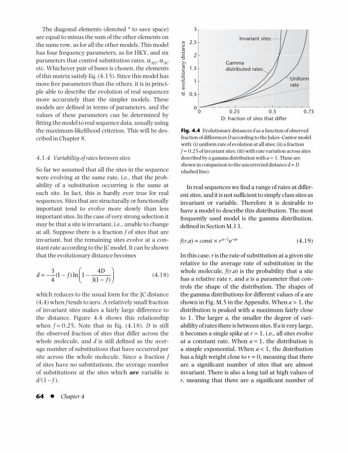
The diagonal elements (denoted * to save space)are equal to minus the sum of the other elements onthe same row, as for all the other models. This modelhas four frequency parameters, as for HKY, and sixparameters that control substitution rates, αAG, αACetc. Whichever pair of bases is chosen, the elementsof this matrix satisfy Eq. (4.15). Since this model hasmore free parameters than the others, it is in princi-ple able to describe the evolution of real sequencesmore accurately than the simpler models. Thesemodels are defined in terms of parameters, and thevalues of these parameters can be determined byfitting the model to real sequence data, usually usingthe maximum-likelihood criterion. This will be des-cribed in Chapter 8.

4.1.4 Variability of rates between sites

So far we assumed that all the sites in the sequencewere evolving at the same rate, i.e., that the prob-ability of a substitution occurring is the same at each site. In fact, this is hardly ever true for realsequences. Sites that are structurally or functionallyimportant tend to evolve more slowly than lessimportant sites. In the case of very strong selection itmay be that a site is invariant, i.e., unable to changeat all. Suppose there is a fraction f of sites that areinvariant, but the remaining sites evolve at a con-stant rate according to the JC model. It can be shownthat the evolutionary distance becomes

(4.18)

which reduces to the usual form for the JC distance(4.4) when f tends to zero. A relatively small fractionof invariant sites makes a fairly large difference tothe distance. Figure 4.4 shows this relationshipwhen f = 0.25. Note that in Eq. (4.18), D is still the observed fraction of sites that differ across thewhole molecule, and d is still defined as the aver-age number of substitutions that have occurred persite across the whole molecule. Since a fraction fof sites have no substitutions, the average number of substitutions at the sites which are variable is d/(1 − f ).

d fD

f ( ) ln

( )= − − −

−⎛⎝⎜

⎞⎠⎟

34

1 14

3 1

In real sequences we find a range of rates at differ-ent sites, and it is not sufficient to simply class sites asinvariant or variable. Therefore it is desirable tohave a model to describe this distribution. The mostfrequently used model is the gamma distribution,defined in Section M.13.

f(r,a) = const × r a−1e−ar (4.19)

In this case, r is the rate of substitution at a given siterelative to the average rate of substitution in thewhole molecule, f(r,a) is the probability that a sitehas a relative rate r, and a is a parameter that con-trols the shape of the distribution. The shapes of the gamma distributions for different values of a areshown in Fig. M.5 in the Appendix. When a > 1, thedistribution is peaked with a maximum fairly closeto 1. The larger a, the smaller the degree of vari-abililty of rates there is between sites. If a is very large,it becomes a single spike at r = 1, i.e., all sites evolve at a constant rate. When a = 1, the distribution is a simple exponential. When a < 1, the distributionhas a high weight close to r = 0, meaning that thereare a significant number of sites that are almostinvariant. There is also a long tail at high values of r, meaning that there are a significant number of

64 l Chapter 4

0 0.25 0.5 0.75D: fraction of sites that differ

0

0.5

1

1.5

2

2.5

3

d: e

volu

tiona

ry d

ista

nce

Invariant sites

Gammadistributed rates

Uniformrate

Fig. 4.4 Evolutionary distances d as a function of observedfraction of differences D according to the Jukes–Cantor modelwith: (i) uniform rate of evolution at all sites; (ii) a fraction f = 0.25 of invariant sites; (iii) with rate variation across sitesdescribed by a gamma distribution with a = 1. These areshown in comparison to the uncorrected distance d = D(dashed line).

BAMC04 09/03/2009 16:42 Page 64

sites that evolve much more rapidly than average.The evolutionary distance for the JC model when agamma distribution of rates is introduced is

(4.20)

This function is also shown in Fig. 4.4 for the casewhere a = 1. It can be seen that both the invariantsites model and the gamma distribution model givehigher estimates of the mean number of subtitutionsper site for any given observed difference D than thestandard model of constant evolutionary rates.Thus, if we ignore rate variability we get a system-atic underestimation of the evolutionary distance.The effect is small if the distance is small, but itbecomes very large for higher distances. This is ofpractical importance, if we are interested in estimat-ing dates of splits between groups on a phylogenetictree. Yang (1996) gives an instructive example ofthe way the estimated divergence times betweenhumans and various apes depend on rate variability.

The gamma function is used because by introduc-ing only one extra parameter to the model, a, we areable to describe a variety of situations from very littleto very large amounts of rate variability betweensites. There is no reason why the distribution of ratesin a real sequence should obey the gamma distribu-tion exactly, but the function is sufficiently flexiblethat it can fit real data quite well. The optimal valueof a to fit a real data set can be found by maximumlikelihood. For more details, see Yang (1996) andreferences therein.

4.2 THE PAM MODEL OF PROTEINSEQUENCE EVOLUTION

4.2.1 Counting amino acid substitutions

Whereas for a model of DNA sequence evolution weneed a 4 × 4 matrix, for a model of protein sequenceswe need a 20 × 20 matrix to account for substitutionsbetween all the amino acids. The original substi-tution rate matrices for amino acids were termedPAM matrices, where PAM stands for “point acceptedmutation”. An accepted mutation is one that spreads

d a D a (( / ) )/= − −−3

41 4 3 11

through the population and goes to fixation. Per-haps a better name for a PAM would be a singleamino acid substitution; however, the term PAM iswell established, and we stick to it here. The follow-ing derivation of the PAM model of amino acid sub-stitutions follows that given by Dayhoff, Schwartz,and Orcutt (1978). At that time, relatively few pro-tein sequences were available. Several groups havesince used much larger data sets to derive improvedPAM models, but the methods used have remainedsimilar. Dayhoff, Schwartz, and Orcutt made align-ments of 71 families of closely related proteins.Sequences in the same family were not more than15% different from one another. They constructedan evolutionary tree for each family using the par-simony method. Parsimony is described in Section8.7, but the principle is straight-forward to statehere – the selected tree is the one that minimizes thetotal number of amino acid substitutions required.

As an example, consider the short protein align-ment shown in Fig. 4.5. This is based on a real pro-tein alignment, but in order to keep the examplesimple, sites have been chosen so that only six of theamino acids occur. The evolutionary tree is alsoshown. The sequences A–G on the tips of the tree areknown, but the sequences 1–5 are chosen by a com-puter program in order to minimize the total numberof substitutions over the whole tree. The requiredsubstitutions are labeled in Fig. 4.5 on the brancheswhere they occur.

Having determined all the substitutions, weobtain a matrix whose elements, Aij, are the numberof times that amino acid i is substituted by aminoacid j. The parsimony method does not tell us inwhich direction a change occurred (because it pro-duces unrooted trees – see Section 8.1). Thereforewhen a change between i and j is observed, we addone to both Aij and Aji. In the example, there is achange between a K and a T on the branch betweennodes 2 and 3. If the root of the tree is as shown inFig. 4.5, then this change is from K to T; however, ifthe root had been drawn such that sequence G werethe outgroup then the change would be from T to K.We thus count one change in both directions. In theexample there are a total of seven substitutions andthe following Aij matrix results:

Models of sequence evolution l 65

BAMC04 09/03/2009 16:42 Page 65

I K L Q T VI – – 2 – 1 1K – – – 1 1 –L 2 – – – – – (4.21)Q – 1 – – 1 –T 1 1 – 1 – –V 1 – – – – –

The Aij matrix obtained by Dayhoff et al. (1978)involved all 20 amino acids and had 1572 substi-tutions. In some cases it is equally parsimonious for more than one different amino acid to occur onan internal node. Where the internal node sequ-ences were ambiguous, fractional substitutions were

counted for each of the possible changes. Jones,Taylor, and Thornton (1992) carried out a similarmethod using all the sequences then available inSwiss-Prot. They automatically clustered sequencesinto groups of >85% similarity and used a distancematrix method to obtain phylogenetic trees (seeSection 8.3). Their Aij matrix contains 59,190 sub-stitutions and is reproduced in Fig. 4.6 (above thediagonal). All possible interchanges between aminoacids are observed at least once in this large data set.

Another reason why each substitution is countedin both directions when calculating the Aij matrix isthat we are aiming to create a time-reversible modelof evolution, as discussed for DNA models in Section4.1.2. The frequencies of the amino acids πi areassumed to be constant through time on average.Therefore we would expect to see equal numbers ofsubstitutions in both directions between any twoamino acids, i.e., we would expect Aij = Aji on aver-age. The number of observed substitutions from i to jis proportional to the probability πi of being in state imultiplied by the rate rij of change from i to j giventhat we are in state i. If we begin with a symmetricmatrix where Aij is set equal to Aji then the evolu-tionary model derived from it will satisfy Eq. (4.15)and will be time reversible.

4.2.2 Defining an evolutionary model

As with the DNA models, Pij(t) is the probability ofbeing in state j at time t given that we were in state i at time 0. We will define the PAM1 matrix as Mij = Pij(δt), where δt is a small time value known as1 PAM unit. For small times, we can assume that thesubstitution probabilities are proportional to thesubstitution rates (i.e., the probabilites vary linearlywith time for small times). Our estimate of the substi-tution rate is proportional to the number of observedsubstitutions, Aij, divided by the total number oftimes Ni that amino acid i is seen in the data. Hence,

(for i ≠ j) (4.22)

where λ is a constant of proportionality to be deter-mined. We have adopted the convention that Mij and

MA

Nijij

i

= λ

66 l Chapter 4

A: T L K K V Q K T

1: T L K K V Q K T

B: T L K K V Q K T

C: T L K K I Q K Q

2: T L K K I Q K Q

D: I I T K L Q K Q

E: T I T K L Q K Q

4: T I T K L Q K Q

F: T L T K I Q K Q

3: T L T K I Q K Q

5: T L T K I Q K Q

G: T L T Q I Q K Q

A: T L K K V Q K TB: T L K K V Q K TC: T L K K I Q K QD: I I T K L Q K QE: T I T K L Q K QF: T L T K I Q K QG: T L T Q I Q K Q

V IT Q

L II L

K T

K Q

T I

Fig. 4.5 A short protein sequence alignment and thephylogenetic tree obtained for these sequences using theparsimony method. Internal nodes 1–5 are labeled with thededuced amino acid sequence at each point. Amino acidsubstitutions are labeled on the branch where they occur.Trees like this are the first stage of derivation of the PAMmodel.

BAMC04 09/03/2009 16:42 Page 66

rij represent substitutions from i to j in order to beconsistent with the definition of DNA models used inthe previous section, and also with the way the data ofJones et al. (1992) are presented in Fig. 4.6, and withrecent authors such as Adachi and Hasegawa (1996)and Müller and Vingron (2000). Unfortunately theopposite convention was used by Dayhoff et al. (1978);therefore some of the formulae used here have theirindices reversed with respect to the original paper.

The frequency of amino acid i in the data is πi = Ni/Ntot, where Ntot is the total number of aminoacids in the data set. To determine λ we adopt theconvention that 1 PAM unit is the time such that anaverage of 1% of amino acids have changed. Thefraction of sites that have changed is

(4.23)

π π λπ

λi

iij

j i ii

j i

ij

tot i

tot

tot

MA

N

A

N∑ ∑ ∑ ∑≠ ≠

= = = .0 01

where Atot is the total of all the elements in the Aijmatrix. Hence

λ = 0.01Ntot/Atot (4.24)

To complete the specification of the PAM1 matrixwe need to define the probability Mii that amino acidi remains unchanged in a time of 1 PAM unit. This issimply

(4.25)

The PAM1 matrix obtained by Jones et al. (1992)is shown in Fig. 4.7. Values have been multiplied by 100,000 for convenience. This means that thesum of the elements on each row is 100,000. Dia-gonal elements are all slightly less than one, and off-diagonal elements are all very small. The twohighest non-diagonal elements in each row have been

M Mii ijj i

= −≠∑1

Models of sequence evolution l 67

ARNDCQEGHILKMFPSTWYV

A2–100–1–1–11–20–1–1–1–3112–4–31

R247 5 0 –1 –1 2 0 0 2 –3 –3 4 –2 –4 –1 –1 –1 0 –2 –3

N216 116 3 2 –1 0 1 0 1 –2 –3 1 –2 –3–1 1 1 –5 –1 –2

D386 48

1433 5 –3 1 4 1 0 –3 –4 0 –3 –5 –2 0 –1 –5 –2 –2

C106 125 32 13 11 –3 –4 –1 0 –2 –3 –3 –2 0 –2 1 –1 1 2 –2

Q208 750 159 130 9 5 2 –1 2 –3 –2 2 –2 –4 0 –1 –1 –3 –2 –3

E600 119 180

2914 8

1027 5 0 0 –3 –4 1 –3 –5 –2 –1 –1 –5 –4 –2

G1183 614 291 577 98 84

610 5 –2 –3 –4 –1 –3 –5 –1 1 –1 –2 –4 –2

H46 446 466 144 40 635 41 41 6 –3 –2 1 –2 0 0 –1 –1 –3 4 –3

I173 76 130 37 19 20 43 25 26 4 2 –3 3 0 –2 –1 1 –4 –2 4

L257 205 63 34 36 314 65 56 134 1324

5 –3 3 2 0 –2 –1 –2 –1 2

K200 2348 758 102

7 858 754 142 85 75 94 5 –2 –5 –2 –1 –1 –3 –3 –3

M100 61 39 27 23 52 30 27 21 704 974 103

6 0 –2 –1 0 –3 –2 2

F51 16 15 8 66 9 13 18 50 196 1093

7 49 8 –3 –2 –2 –1 5 0

P901 217 31 39 15 395 71 93 157 31 578 77 23 36 6 1 1 –4 –3 –1

S2413 413 1738 244 353 182 156 1131 138 172 436 228 54 309 1138

2 1 –3 –1 –1

T2440 230 693 151 66 149 142 164 76 930 172 398 343 39 412 2258

2 –4 –3 0

W11 109

2 5 38 12 12 69 5 12 82 9 8 37 6 36 8 15 0 –3

Y414611489164401515514618420178502216445419–3

V1766

6955127995822627622

39381261

585591898421952627424

Fig. 4.6 Above the diagonal – numbers of observed substitutions, Aij, between each pair of amino acids in the data of Jones,Taylor, and Thornton (1992). On and below the diagonal – log-odds scoring matrix corresponding to PAM250 calculated fromthese data. This is calculated as Sij = 10 log10 Rij and rounded to the nearest integer. Cells shaded gray have positive scores,meaning that these amino acids are more likely to interchange than would be expected by chance. Values written in white on ablack box correspond to amino acid substitutions that are possible via a single nucleotide substitution at one position in the codon.

BAMC04 09/03/2009 16:42 Page 67

highlighted in black. These are the two highest sub-stitution rates for each amino acid, e.g., A is morelikely to change to S and T than to the other aminoacids. We will consider more fully why some ratesare much larger than others in the section on logodds matrices. For now we note that, unlike the Aij matrix, the Mij matrix is not symmetric. This isbecause the frequencies of the amino acids are notequal. The values of the amino acid frequencies in the data of Jones et al. are given in Fig. 4.7. As this model is time reversible we have πiM ij = πj Mji.So for amino acids A and V, for example, we have0.077 × 0.00193 = 0.066 × 0.00226 = 0.000149.

Since PAM1 corresponds to an average probab-ility of 0.01 of amino acids changing, we would

expect all the diagonal elements to be 0.99 (i.e.,99,000 on the figure) if each amino acid changed at the same rate. However, some amino acids aremore likely to undergo substitutions than others.Amino acids that change more rapidly than aver-age will have a probability lower than 0.99 of re-maining unchanged after a time of 1 PAM, whereasthose that change more slowly than average willhave a probability higher than 0.99 of remain-ing unchanged. Using Eq. (4.22), the total prob-ability of substitution from amino acid i to any otheramino acid in a time of 1 PAM unit is 1 − Mii. If wedivide this by the mean substitution probability0.01, we obtain the relative mutability mi of aminoacid i:

68 l Chapter 4

A

R

N

D

C

Q

E

G

H

I

L

K

M

F

P

S

T

W

Y

V

A

98759

41

43

63

44

43

82

135

17

28

24

28

36

11

150

297

351

7

11

226

R

27

98962

23

8

52

154

16

70

164

12

19

334

22

3

36

51

33

65

12

9

N

24

19

98707

235

13

33

25

33

171

21

6

108

14

3

5

214

100

1

30

7

D

42

8

284

98932

5

27

398

66

53

6

3

14

10

2

7

30

22

3

23

16

C

12

21

6

2

99450

2

1

11

15

3

3

1

8

14

3

44

9

23

43

13

Q

23

125

31

21

4

98955

140

10

223

3

29

122

19

2

66

22

21

7

10

7

E

66

20

36

478

3

211

99042

70

15

7

6

107

11

3

12

19

20

7

4

29

G

129

102

58

95

41

17

83

99369

15

4

5

20

10

4

16

139

24

41

4

35

H

5

74

92

24

17

130

6

5

98867

4

12

12

8

11

26

17

11

3

134

3

I

19

13

26

6

8

4

6

3

10

98722

122

11

253

41

5

21

134

7

16

504

L

28

34

12

6

15

64

9

6

49

212

99328

13

350

230

97

54

25

49

22

161

K

22

390

150

17

3

176

102

16

31

12

9

99101

37

1

13

28

57

5

5

7

M

11

10

8

4

10

11

4

3

8

113

90

15

98845

10

4

7

49

5

4

71

F

6

3

3

1

28

2

2

2

18

31

101

1

18

99357

6

38

6

22

222

24

P

99

36

6

6

6

81

10

11

58

5

53

11

8

8

99278

140

59

4

6

11

S

264

69

344

40

147

37

21

129

51

28

40

32

19

65

190

98548

325

21

43

28

T

267

38

137

25

28

31

19

19

28

149

16

57

123

8

69

278

98670

5

12

67

W

1

18

0

1

16

2

2

8

2

2

8

1

3

8

1

4

1

99684

11

3

Y

4

8

23

15

68

8

2

2

189

10

8

3

6

179

4

20

6

24

99377

5

V

193

11

11

21

41

12

31

32

8

630

117

8

201

40

14

27

76

16

11

98772

πI

mi

A

0.077

1.241

R

0.051

1.038

N

0.043

1.293

D

0.052

1.068

C

0.020

0.550

Q

0.041

1.045

E

0.062

0.958

G

0.074

0.631

H

0.023

1.133

I

0.053

1.273

L

0.091

0.672

K

0.059

0.899

M

0.024

1.155

F

0.040

0.643

P

0.051

0.722

S

0.069

1.452

T

0.059

1.330

W

0.014

0.316

Y

0.032

0.623

V

0.066

1.228

Fig. 4.7 PAM1 matrix calculated by Jones, Taylor, and Thornton (1992). Values are multiplied by 105 for convenience. Mij isthe probability that the amino acid in row i changes to the amino acid in column j in a small time corresponding to 1 PAM unit.The two highest non-diagonal elements in each row are highlighted in black. These are the two most rapid substitution rates foreach amino acid. Frequencies πi and relative mutabilities mi of each amino acid are shown at the bottom of the figure.

BAMC04 09/03/2009 16:42 Page 68

mi = (1 − Mii)/0.01 (4.26)

The relative mutabilities are given at the foot ofFig. 4.7. A relative mutability of 1 corresponds to anamino acid that changes at the average rate. Theleast mutable amino acid is tryptophan (W) withmutability mW = 0.316, which is less than a third ofthe average rate. The most mutable amino acid isserine (S) with mS = 1.452. The mutability valuesreflect important properties of the amino acids (seeSection 4.3.2 below). Note that Jones et al. (1992)and Dayhoff et al. (1978) used a different scale forrelative mutabilities where the mutability of alanineis set to 100. The scale used here seems more logicalbecause there is nothing special about alanine.

4.2.3 Extrapolating the model to higher distances

The PAM1 matrix in Fig. 4.7 is the equivalent of oneof the evolutionary models for DNA discussed inSection 4.1, except that the Mij matrix represents atransition probability in a small discrete unit of time,whereas the rate matrices rij represent rates ofchange in a continuous time model. For two aminoacids that are not equal, the probability of substitu-tion for a small time δt is

Pij(δt) = δt × rij = Mij (4.27)

while the probability of remaining unchanged is

Pii(δt) = = Mii (4.28)

Choosing the value of λ above is equivalent to choos-ing a value of δt so that there is a probability of 1% ofan amino acid changing in this time.

Now suppose we want to obtain the transitionprobabilities for time 2δt. It is not true that Pij(2δt) =2Mij. In order to calculate this probability we need toconsider all the intermediate states that could haveexisted at time δt, and sum over them:

Pij(2δt) = (4.29)

Thus if we want to get from A to V in two steps, wecan go A→A→V, or A→V→V, or A→R→V, or any

M Mik kj

k∑

1 − ×≠∑δt rijj i

of the other 17 possibilities. To calculate Pij(nδt) wehave to sum over the possible amino acids that couldoccur at the n − 1 intermediate time points. To dothis we have to multiply the M matrix by itself ntimes to obtain the matrix Mn and take the ij elementof this matrix. This is written:

(4.30)

where there are n − 1 indices to be summed over.This completes the derivation of the PAM model.

The substitution probability matrices known asPAM100, PAM250, etc. are simply the PAM1matrix M multiplied by itself 100 or 250 times. It isstraightforward to calculate these matrices by com-puter. The number of times we multiply the matrix iscalled the PAM distance. Box 4.2 gives more infor-mation about PAM distances.

The method for deriving the PAM model beganwith groups of closely related sequences. This isimportant for several reasons. When sequences aresimilar, it is easy to align them because there arealmost no gaps. In this case the alignment is veryinsensitive to the scoring matrix we use – if we havenot yet derived a good scoring matrix we do notwant the alignments used to be sensitive to thedetails of the rather poor scoring matrix we use toalign them. In addition, constructing phylogenetictrees is generally more reliable for more closelyrelated sequences. The parsimony method weightseach type of amino acid substitution equally whenchoosing the tree. Again, this avoids using an evolu-tionary model that has yet to be calculated. Whencounting the substitutions, it is assumed that nomore than one substitution has occurred per site onany branch. For example, the K↔T substitutionbetween nodes 2 and 3 in Fig. 4.5 is assumed to be adirect change and not via an intermediate routesuch as K↔Q↔T. If sequences are similar to oneanother, this is a reasonable assumption, but formore distant sequences, there is no reason thisshould be true and there would be little justificationfor using parsimony. Likelihood-based methods ofestimating substitution matrices that avoid thisproblem are discussed in Section 11.2.2.

P n t M M M Mijn

k lik

mkl mj( ) . . . . . . δ = = ∑ ∑ ∑

Models of sequence evolution l 69

BAMC04 09/03/2009 16:42 Page 69

70 l Chapter 4

BOX 4.2PAM distances

For two proteins at a PAM distance of 1, there have beenan average of 0.01 substitutions per site, and the prob-ability that two sites in the aligned pair of proteins willdiffer is D = 0.01. For two proteins at a PAM distance n,there have been an average of 0.01 × n substitutions persite. To keep parallel with DNA models, where evolution-ary distances are usually defined as d = number of substi-tutions per site, we will define d = 0.01 × n for the PAMmodel. So PAM100 corresponds to an average of d = 1substitution per site. However, it does not follow that allsites have changed exactly once, because there will havebeen more than one change in some places and nochanges in other places. In fact, the fraction of sites thatdiffer at a PAM distance n is

(4.31)

This is just the probability that the amino acid in thefirst sequence is an i multiplied by the probability thatthe amino acid in the second sequence has notremained an i after n PAM units of time. This formulagives us a relationship between the observed fraction ofsites that differ, D, and the evolutionary distance, d. It isthus the equivalent of Eq. (4.4) for the Jukes–Cantor dis-tance in the model of DNA evolution. In Fig. 4.8 we haveplotted this relationship using the data in Table 23 ofDayhoff et al. (1978). The curve has a similar shape tothe curve for the DNA models in Fig. 4.4: it is linear forsmall D, and diverges for larger D. The value of D forunrelated proteins tends to about 0.89. This figure tellsus that at d = 1 (or PAM distance 100) D = 0.57 or, inother words, there are still 43% of residues that will bethe same even though there has been an average of onesubstitution per site.

As it stands, the distance formula (4.31) is much lessuseful than the one for the JC model. If we have twoaligned proteins, we can easily calculate D, but it is notimmediately obvious how to calculate the PAM distanced using this equation. One solution is to use the graph in Fig. 4.8 as a “calibration curve”. For example, if weobserve a fraction D = 0.5, then we can deduce that d = 0.8 substitutions per site (i.e., PAM distance = 80).To avoid having to use the graph, Kimura (1983)showed that the relationshipd = −ln(1 − D − 0.2D2) (4.32)

D Mi ii

n

i

( )= −∑ π 1

is extremely close to the curve calculated from theDayhoff data over most of the range of PAM distances.Thus, the dashed line in Fig. 4.8 is almost indistinguish-able from the solid line for D less than about 0.75. Thisequation can be used directly to calculate distancesbetween proteins because it is “the right way round”.

However, both Eqs. (4.31) and (4.32) apply only tovery long sequences where the frequencies of all theamino acids are assumed to be equal to the average fre-quencies in the Dayhoff data. For two real proteins offinite length, the amino acid frequencies will not beexactly equal to the average frequencies. A more preciseway to estimate distance uses maximum likelihood. Fortwo sequences of length L, let ak and bk be the aminoacids at the kth site in sequences 1 and 2, respectively.The likelihood of sequence 1 evolving into sequence 2 inn PAM units is

(4.33)

The maximum likelihood value of the PAM distance isthe value of n that maximizes L(n), and the maximumlikelihood value of the number of substitutions per site is d = n/100. As an example, we calculated evolution-ary distances between a set of hexokinase sequencesusing the “protdist” program in the Phylip package(Felsenstein 2001). These sequences will be discussed inmore detail in Section 6.5 on multiple alignment. Fordistance estimates, an alignment of 393 sites was usedwith all gap regions eliminated. In Fig. 4.8, the datapoints show the maximum likelihood evolutionary dis-tance between one sequence (HXK1_RAT) and each ofthe other sequences in the alignment. These data pointslie approximately on the average curve but not exactly.

There are many ways of estimating distances betweenproteins, and it is necessary to read the details of themethod employed in any program that one uses.Evolutionary models calculated from different sequencesets give slightly different distances from those using theDayhoff et al. (1978) PAM model. It is also worth notingthat the distances given by the Tree-Puzzle program(Schmidt et al. 2000) are not exactly the same as thosegiven by the Phylip protdist program, even when thesame Dayhoff PAM model is used. This is because Phylipassumes the equilibrium amino acid frequencies are fixedas in the original data, whereas Tree-Puzzle re-estimatesthese frequencies from the data.

L n Ma

k

L

a bn

k k k( ) =

=∏ π

1

BAMC04 09/03/2009 16:42 Page 70

4.3 LOG-ODDS SCORING MATRICESFOR AMINO ACIDS

4.3.1 PAM scoring matrices

We will now describe the way in which the PAMmodel of evolution can be used to derive scoringmatrices for use in protein sequence alignment.Consider two very long proteins that are n PAMunits apart. The fraction of sites at which the firstsequence has amino acid i and the second has aminoacid j is πi M

nij. Now suppose we randomly reshuffle

the amino acids in each sequence. The frequency ofthe amino acids remains the same but there is nolonger any evolutionary relationship between thesequences. The fraction of sites at which the firstsequence is i and the second sequence is j is now justπi πj. We define Rij as the ratio of these two values:

(4.34)

Thus Rij is the ratio of the number of times that an i isaligned with a j in proteins evolving according to thePAM model to the number of times that an i wouldbe aligned with a j in random protein sequences with

RM M

iji ij

n

i j

ijn

j

= =ππ π π

the same amino acid frequencies. If Rij > 1, thenamino acids i and j are more likely to be aligned witheach other according to the PAM model than theywould be by chance. Because the PAM model is time reversible, the matrix of R values is symmetric(Rij = Rji). This is common sense because the prob-ability that an i and a j are aligned with each othercannot depend on which of the two sequences wecall sequence 1 and which we call sequence 2. Letthe amino acids at the kth site in the two proteins be ak and bk, as in Box 4.2. The relative likelihood ofthis pair of aligned sequences arising according tothe PAM model to the likelihood of the pair arising if the amino acids were chosen at random is

relative likelihood = (4.35)

When deciding how to align two proteins, weshould choose the alignment that maximizes thisrelative likelihood, i.e., we should choose the align-ment that is most likely to arise according to our evolutionary model. Algorithms for calculating theoptimum alignment will be discussed in Chapter 6.For these algorithms, it is convenient to have analignment score that is a sum over sites, rather than

Ra b

k

L

k k=

∏1

Models of sequence evolution l 71

1.2

1.6

2.0

2.4

0

0.4

0.8

0 0.20.1 0.40.3Fraction of sites that differ (D)

0.5 0.6 0.7 0.8 0.9

Evol

utio

nary

dis

tanc

e (d

)

Fig. 4.8 The relationshipbetween the evolutionarydistance d and the fraction ofsites that differ D according tothe PAM model of evolution.Solid line, the empiricalrelationship calculated fromDayhoff et al. (1978) data (Eq.(4.31)); dashed line, the Kimuradistance formula (Eq. (4.32)).Data points are calculated by thePhylip package for a particularset of aligned proteins using thesame evolutionary model.

BAMC04 09/03/2009 16:42 Page 71

a product over sites like Eq. (4.35). To derive thesescores, we just take logs of the Rij values. The scorefor alignment of amino acid i with amino acid j is

S(i,j) = C logB Rij (4.36)

B is the base of logarithm that we choose to take, andC is any arbitrary constant. These two constants are chosen so that the scores are on a convenientscale. We can write the score for alignment of thetwo sequences (forgetting about gaps for the mom-ent) as

alignment score = (4.37)

The alignment that maximizes the sum in Eq. (4.37)is the same as the alignment that maximizes the relative likelihood in Eq. (4.35).

Leaving the alignment problem until Chapter 6,let us now think more carefully about what thesescores mean. A matrix of scores calculated accord-ing to Eq. (4.36) is called a log-odds matrix. The log-odds matrix calculated for PAM250 using thedata of Jones et al. (1992) is shown in Fig. 4.6 (belowthe diagonal). In this case both B and C are 10, andthe values shown are rounded to the nearest integer.Positive scores indicate that the two amino acids aremore likely to be aligned with one another than theywould be by chance, and negative scores mean thatthey are less likely to be aligned with one anotherthan they would be by chance. Positive scores areshaded gray. Note that all the diagonal elements areshaded, meaning that each amino acid is more likelyto be aligned with itself than it would be by chance.The highest score is S(W,W) = 15. To see what thismeans, we can invert Eq. (4.36) to give Rij = BS(i,j)/C.In this case we have RWW = 1015/10 = 31.6, meaningthat a W is 31.6 times more likely to be aligned withanother W in proteins at PAM distance 250 than itwould be by chance. This reflects the fact that W hasa very low relative mutability – see Eq. (4.26) above.Similarly, amino acids with high mutability like Shave low scores on the diagonal, meaning that an Sis only slightly more likely to be aligned with itselfthan it would be by chance.

S a bk

k

L

k( , )=∑

1

4.3.2 Relationship to the physico-chemical propertiesof amino acids

The shaded off-diagonal elements in Fig. 4.6 are thehighest scores between non-identical amino acids.These are the pairs of amino acids that are mostlikely to be aligned with one another. They tend to bepairs that have similar physico-chemical properties.The few highest-scoring pairs are listed here.• Y↔F. Tyrosine and phenylalanine both have anaromatic side group and differ only by the presenceof an OH group on the benzene ring in tyrosine.• D↔E. Aspartate and glutamate both have anacidic COO− group and differ only by the presence ofan extra carbon in the side chain of glutamate.• K↔R. Lysine and arginine are both basic andhave relatively long side chains ending in positivelycharged NH 3

+ or NH 2+ groups.

• V↔I. Valine and isoleucine are both hydropho-bic amino acids with medium-sized hydrocarbonside chains. They differ by a single extra carbon inisoleucine.

In contrast, amino acids that have differentphysico-chemical properties tend to have negativescores. For example, most scores between hydro-philic and hydrophobic amino acids are negative. Itis also noticeable that the two most slowly evolvingamino acids, tryptophan and cysteine, have ratherunusual physico-chemical properties. Tryptophan is the largest amino acid with a very bulky sidechain. If it is substituted by another side chain it is likely that this will cause a substantial change inthe 3D structure of the protein. Hence it will mostlikely be a deleterious mutation that will be elimin-ated by selection. Cysteine residues have the abilityto form disulfide bonds, C–S–S–C, between differentparts of protein chains. The disruption of thesebonds would also be likely to cause a major effect on the protein structure. Thus, the observed rate ofsubstitutions involving both W and C is small. Theseamino acids have high scores on the diagonal butnegative scores for alignment with almost every-thing else.

We spent a long time discussing the properties ofamino acids in Chapter 2. The plot from principalcomponent analysis (Fig. 2.10) is a good way of

72 l Chapter 4

BAMC04 09/03/2009 16:42 Page 72

summarizing the differences in the amino acid prop-erties. Almost all the pairs of amino acids with highPAM scores are close to one another on the PCA plot.To see this, try making a copy of Fig. 2.10 and joining all the pairs of points corresponding to theshaded cells in Fig. 4.6. This confirms the fact thatevolution does take notice of amino acid properties.It also confirms what we said in Chapter 3 regardingthe stabilizing action of natural selection, i.e., selec-tion is acting against mutations that change theamino acid properties too drastically, and prevent-ing these changes reaching fixation. The only sig-nificantly positive scores in the PAM matrix thatappear quite far from one another on the PCA plotare CW and CY. We already said that cysteine is anunusual amino acid that cannot easily be replacedby anything else. The explanation for the high PAMscores for CW and CY is probably due to the proxim-ity of these amino acids in the genetic code, as wenow describe, rather than because of similarities inphysico-chemical properties.

Examination of Fig. 4.6 reveals that the structureof the genetic code also has a role in the rates ofamino acid substitution. As can be seen from thegenetic code diagram in Table 2.1, it is possible forsome substitutions of amino acids to occur by thesubstitution of a single nucleotide at one of the threepositions in the codon, whereas other amino acidsubstitutions require more than one nucleotide sub-stitution. We would expect the amino acid substitu-tions that require only one nucleotide substitutionto occur more rapidly. In Fig. 4.6, the scores for theamino acid pairs that can be substituted with a sin-gle nucleotide change are highlighted in a black box.It can be seen that all the pairs with positive scores(gray cells) are also highlighted in black. Therefore,there is no substitution that is frequently observedthat cannot be achieved by a single nucleotidechange. However, there are many zero or negativescores that are also shaded black. Thus, not all thesubstitutions that are possible via a single nucleotidechange are frequently observed. This shows that theeffect of the genetic code is moderated by the actionof natural selection on the amino acid proper-ties. For example, the substitution from valine (V) to glutamate (E) is possible by a single nucleotide

substitution from T to A at the second position. Thispresumably occurs frequently as a mutation in thepopulation. However, selection is likely to eliminatemost of these changes because the physico-chemicalproperties of the amino acids are too different. Theobserved rate of V↔E substitutions is therefore lowbecause most of these mutations do not go to fixa-tion, and the score S(V,E) is negative.

As an interesting aside, it appears that the struc-ture of the genetic code is far from random. It is oftenthe case that amino acids with similar properties are next to one another in the diagram (Table 2.1)and therefore that they are accessible by a singlenucleotide change. As a result the average effect ofrandom point mutations on the physico-chemicalproperties of a protein is less than one might expect.This has been shown by comparing the real codewith many possible randomly reshuffled geneticcodes (Freeland et al. 2000). It is therefore arguedthat the code has evolved by reshuffling the assign-ment of codons to amino acids in order to minimizeerrors. Although the canonical code is thought tohave arisen very early in evolution (before the splitof archaea, bacteria, and eukaryotes), and althoughthe process of codon reassignment is potentially verydisruptive to an organism, there are neverthelessmany small changes to the code that have occur-red in isolated groups of organisms or organelles since the canonical code was established (Knight,Freeland, and Landweber 2001). Thus reshuffling ofthe code due to selection for error minimization inthe early stages of life on earth is not impossible.

Returning to scoring matrices, we note that a log-odds matrix can be derived for any PAM distance.The PAM250 matrix shown in Fig. 4.6 represents arelatively large distance. This means that there is asubstantial chance that an amino acid has changedand therefore there are a fairly large number of positive scores in the off-diagonal elements. For asmaller PAM distance like 100 or less, there wouldbe a higher probability that each amino acid hadremained unchanged. Therefore the scores on thediagonal of the matrix would be larger, and most ofthe off-diagonal scores would be negative. The PAMscoring matrices are used for pairwise sequencealignments and for database searches. The matrices

Models of sequence evolution l 73

BAMC04 09/03/2009 16:42 Page 73

are most effective at spotting similarities betweensequences that are at evolutionary distances com-parable with the PAM distance of the matrix. LowPAM number matrices are used to spot matcheswith a high percentage identity between the sequ-ences. High PAM number matrices are used to spotmatches between distantly related sequences, wherethe residues may not be identical but the physico-chemical properties of the amino acids are con-served. Examples of alignments and database searchresults using different PAM matrices are discussed inChapters 6 and 7.

4.3.3 BLOSUM scoring matrices

The BLOSUM matrices (Henikoff and Henikoff1992) are another set of log-odds scoring matricesthat have much in common with PAM matrices,although they are derived in a different way. In particular, the scoring matrix is derived directlyfrom sequence alignments without the use of a phy-logenetic tree, and without deriving an evolutionarymodel.

The basics of the method can be explained usingthe sequence alignment in Fig. 4.5. First we countthe number of times each amino acid appears andhence obtain the frequencies πi of each amino acid inthe data set. Then we count the number of times Aijthat each amino acid is aligned with each otheramino acid. In Fig. 4.5 there are seven sequences.The total number of ways of picking a pair of aminoacids from one column of the alignment is 7 × 6 =42. The seventh column of the alignment is all K.This column contributes 42 to AKK. In the first col-umn of the alignment we have six Ts and one I. Thiscolumn contributes 6 × 5 = 30 to A TT, six to ATI andsix to AIT. When the totals from all the columns areadded, the following matrix Aij results:

I K L Q T VI 8 – 16 – 6 6K – 78 – 6 12 –L 16 – 22 – – 4 (4.38)Q – 6 – 62 10 –T 6 12 – 10 44 –V 6 – 4 – – 2

This differs from the Aij matrix calculated by thePAM method (Eq. (4.21)) in that we are countingpairs of aligned amino acids instead of numbers ofsubstitutions. Thus we have non-zero entries on thediagonal. There are also some entries like AVL thatare non-zero in Eq. (4.38) but are zero in Eq. (4.21).This is because V and L amino acids are aligned witheach other at site 5, whereas the parsimony methodused in Fig. 4.5 found that there were substitutionsV↔I and I↔L at site 5 but no direct substitutionV↔L. The two methods treat the same alignmentdata in different ways and thus result in differentscoring matrices.

We can now obtain the fraction of aligned pairsthat are of type ij:

(4.39)

where Atot is the total of all the elements in the Aijmatrix. From this we can directly obtain the relativefrequency of ij pairs in the aligned proteins com-pared with what we would expect for randomlyreshuffled proteins with the same base frequencies:

(4.40)

This quantity Rij is directly comparable to the Rij thatwe calculated for the PAM model in Eq. (4.34). Wecan use it to calculate a log-odds scoring systemusing Eq. (4.36) in the same way.

The mathematics of this method is much simplerthan for the PAM method because we can go directlyfrom the data to the log-odds matrix without need-ing to derive an evolutionary model (Mij) first. Thereare nevertheless some disadvantages. The resultthat we obtain is sensitive to the presence of groupsof very closely related sequences in the alignment.These sequences will be almost identical and willcontribute a large amount to the numbers on thediagonal of the Aij matrix. In contrast, groups ofalmost identical sequences do not affect the PAMmethod because these appear very close to oneanother on the phylogenetic tree and very few sub-stitutions are required on these branches of the tree.Real sequence data are usually obtained in a very

Rq

ijij

i j

=π π

qA

Aijij

tot

=

74 l Chapter 4

BAMC04 09/03/2009 16:42 Page 74

“patchy” way, with a lot of sequences available for afew well-studied groups and only a few sequencesavailable from other groups. It is therefore necessaryto develop a systematic way of accounting for thedistribution of distances between the sequences inthe alignments used for the BLOSUM method.

Henikoff and Henikoff (1992) used alignments ofprotein domains from the Blocks database (see Section5.5.5). These are reliably aligned regions of proteinswithout gaps. Within each alignment sequenceswere grouped into clusters that have a percentageidentity greater than a certain cut-off value (e.g.,80% or 62%). When counting the number of pairedamino acids for the Aij matrix, sequences in the samecluster are not counted. When counting pairsbetween clusters, sequences in the same cluster areweighted as a single sequence (i.e., if there were twoclustered sequences, each would count half theweight of a single distinct sequence). The log-oddsmatrix that results from clustering sequences at agiven percentage is known as the correspondingnumber BLOSUM matrix. Hence BLOSUM80 onlyincludes substitutions between sequences that areless than 80% similar, and BLOSUM62 only includessubstitutions between sequences that are less than62% similar. Lower BLOSUM number therefore rep-resents lower similarity, whereas lower PAM numberrepresents greater similarity.

The scaling of the scores used in BLOSUM62 isS(i,j) = 2 log2Rij. This means that the scores are in“half-bit” units. A bit is a factor of two, and a score of1 in the matrix corresponds to a factor of in re-lative likelihood. The highest score is S(W,W) = 11,which corresponds to RWW = 211/2 = 45.2. This is not too different from what we got with PAM250.Table 4.1 compares three log-odds scoring systemsderived by different methods and using different sets

2

of sequence alignments. The numerical details of thescoring systems are different, hence if we use themfor sequence alignments, we may obtain slightly dif-ferent results. However, the most important featuresof these scoring matrices are the same. The sets ofthe most conserved and least conserved amino acidsand the most significant positive scores betweennon-identical amino acids are very similar in thethree cases. This gives us confidence that the scoringsystems are really calculating something funda-mental about the process of protein sequence evolu-tion and the way in which natural selection acts onthe physico-chemical properties of the amino acids.

When we are searching for similarities betweensequences, it is easy to spot sequences that are verysimilar. The difficulty arises in spotting relationshipsin the “twilight zone” of sequence similarity wherethe resemblance between the sequences is onlyslight. It has been argued that the BLOSUM series of matrices is more effective for use in databasesearch algorithms than the PAM series because it isbased directly on comparison of distant sequences(Henikoff and Henikoff 1993). The PAM method, onthe other hand, counts substitutions in closelyrelated sequences only, and then predicts what willhappen for more distant sequences by extrapolationof the evolutionary model to longer times. It may bethat this extrapolation is not very reliable (Benner,Cohen, and Gonnet 1994). The disadvantage ofBLOSUM is that since it is not based on an evolu-tionary model it cannot be used for calculating evolutionary distances and phylogenetic trees. The reason that the PAM matrix only uses similarsequences is because it relies on parsimony to countthe substitutions. Maximum likelihood methods ofestimating evolutionary models do not have thisrestriction (see Section 11.2.2 for further details).

Models of sequence evolution l 75

BAMC04 09/03/2009 16:42 Page 75

76 l Chapter 4

Runing head l 76

Table 4.1 Important features of amino acid substitution matrices.

Matrix

Most conservedamino acids

Least conservedamino acids

Most significant non-identical matches

JTT250*

1. W2. C3. Y4. F

1. S, A, T2. N3. I, V

1. Y↔F2. V↔I, K↔R, D↔E, Y↔H3. M↔I, M↔L

BLOSUM62**

1. W2. C3. H4. Y, P

1. S, A, I, V, L

1. Y↔F, V↔I2. K↔R, D↔E, Y↔H,L↔I, M↔L, E↔Q, W↔Y

VT160***

1. W2. C3. Y4. F, H, P

1. S, A2. T, I, V, L

1. Y↔F2. V↔I, K↔R3. D↔E, Y↔H, M↔I,M↔L, H↔Q

SUMMARYThe models discussed in this chapter are used todescribe the evolution of a sequence along a branch of aphylogenetic tree. In phylogenetic studies we are notusually interested in sequence variation within a singlespecies and we are using a single sequence to representthe whole species. Therefore the rates of substitution inthe evolutionary models describe the changes in the rep-resentative sequence that arise due to fixation of newalleles. Substitution rates are hence dependent on muta-tion, selection, and drift, and are not simply the rates ofmutation in individual sequences.

DNA sequence evolution can be described by modelsbased on rate matrices having four states: A, C, G, and T.The simplest of these models is the Jukes–Cantor model,where all four bases are assumed to have equal frequ-ency and where all possible substitutions occur at equalrate. More complicated models relax these assumptions.The general reversible model has four parameters for thebase frequencies and six parameters for substitutionrates. It is the most general four-state model that satisfiesthe principle of time reversibility (i.e., that average pro-perties of sequences do not change with time along an evolutionary lineage). The numerical values of theseparameters can be determined by fitting the model to

sequence data, and may not be the same for differenttypes of sequence.

When comparing two sequences it is straightforwardto count the fraction of sites that differ between them, D.However, it is useful to have a measure of evolutionarydistance between sequences that increases linearly withtime at all times. The usual distance measure is d, theaverage number of substitutions per site. Although d isnot directly observable by comparing sequences, it ispossible to calculate d from quantities that are observ-able. This calculation depends on the model of sequenceevolution that is being used. The lengths of branches onphylogenetic trees are often measured in units of substi-tutions per site.

Protein sequence evolution can be described by ratematrices involving 20 states for the 20 amino acids. Itrequires large sets of many sequence alignments todetermine all the parameters in these large matrices. ThePAM model was the first protein evolution model of thistype. The PAM1 subsitution matrix Mij is the probabilityof substitution from amino acid i to j in a time of 1 PAMunit. This is the time in which there is an average of 1%sequence divergence. The probabilities of substitution ina time of n PAM units can be obtained by multiplying thismatrix by itself n times. The PAM distance between two

The most/least conserved amino acids are those with the highest/lowest scores in the diagonals of the log-oddsmatrices. The most significant non-identical matches are the highest off-diagonal scores in the log-odds matrices.Entries are ranked equally when the rounding scheme leads to identical values in the published matrices. * Jones,Taylor, and Thornton (1992) version of PAM250 matrix; ** Henikoff and Henikoff (1992) BLOSUM62; *** Müller andVingron (2000) Variable Time VT160 matrix.

BAMC04 09/03/2009 16:42 Page 76

REFERENCESAdachi, J. and Hasegawa, M. 1996. A model of amino acid

substitution in proteins encoded by mitochondrial DNA.Journal of Molecular Evolution, 42: 459–68.

Benner, S.A., Cohen, M.A., and Gonnet, G.H. 1994.Amino acid substitution during functionally con-strained divergent evolution of protein sequences.Protein Engineering, 7: 1323–32.

Dayhoff, M.O., Schwartz, R.M., and Orcutt, B.C. 1978. Amodel of evolutionary change in proteins. In Atlas ofProtein Sequence and Structure, 5(3): 345–52. Washing-ton DC: National Biomedical Research Foundation.

Felsenstein, J. 2001. PHYLIP Phylogeny Inference Pack-age version 3.6. Available from http://evolution.genetics.washington.edu/phylip.html.

Freeland, S.J., Knight, R.D., Landweber, L.F., and Hurst,L.D. 2000. Early fixation of an optimal genetic code.Molecular Biology and Evolution, 17: 511–18.

Hasegawa, M., Kishino, H., and Yano, T.A. 1985. Datingof the human–ape splitting by a molecular clock of mito-chondrial DNA. Journal of Molecular Evolution, 22:160–74.

Henikoff, S. and Henikoff, J.G. 1992. Amino acid substitu-tion matrices from protein blocks. Proceedings of theNational Academy of Sciences USA, 89: 10915–19.

Henikoff, S. and Henikoff, J.G. 1993. Performance evalu-ation of amino acid substitution matrices. PROTEINS:Structure, Function and Genetics, 17: 49–61.

Jones, D.T., Taylor, W.R., and Thornton, J.M. 1992. Therapid generation of mutation data matrices from proteinsequences. CABIOS, 8: 275–82.

Jukes, T.H. and Cantor, C.R. 1969. Evolution of proteinmolecules. In H.N. Munro (ed.), Mammalian ProteinMetabolism, pp. 21–123. New York: Academic Press.

Kimura, M. 1983. A simple method of estimating evolu-tionary rates of base substitutions through comparativestudies of nucleotide sequences. Journal of MolecularEvolution, 16: 111–20.

Knight, R.D., Freeland, S.J., and Landweber, L.F. 2001.Rewiring the keyboard: Evolvability of the genetic code.Nature Reviews Genetics, 2: 49–58.

Müller, T. and Vingron, M. 2000. Modeling amino acidreplacement. Journal of Computational Biology, 7: 761–76.

Schmidt, H.A., Strimmer, K., Vingron, M., and vonHaeseler, A. 2000. Tree-Puzzle version 5.0 availablefrom http://www.tree-puzzle.de/.

Yang, Z. 1996. Among-site rate variation and its impacton phylogenetic analyses. Trends in Ecology and Evolu-tion, 11: 367–72.

Models of sequence evolution l 77

proteins is an estimate of the number of substitutionsper site, as with DNA sequence distances, although it isconventionally mutiplied by 100. Thus a PAM distanceof n corresponds to n/100 substitutions per site.

The PAM substitution matrices can be used to calcu-late log-odds scoring matrices for use with protein sequ-ence alignment algorithms. The scores S(i,j) are definedas the logarithm of the ratio of the probability that aminoacids i and j are aligned in sequences evolving accordingto the model to the probability that they would be

aligned in random sequences. Positive scores indicatepairs of amino acids that substitute for one another morefrequently than would be expected by chance. Thescores are influenced by the physico-chemical propertiesof the amino acids and also by the structure of thegenetic code. The BLOSUM scoring matrices are anotherset of log-odds matrices that are calculated directly fromsets of sequence alignments without the use of an evolu-tionary model. These matrices can be used for sequencealignments but not for phylogenetics.

BAMC04 09/03/2009 16:42 Page 77

78 l Chapter 4

PROBLEMS

4.1 In Section 4.3.1 we itroduced the Kimura two-parameter model of DNA sequence evolution. The aimof this problem is to guide you through the calculationof the evolutionary distance in this model in a step-by-step way. The result was already given in the text –Eq. (4.13)

Use what you know to eliminate PAG, PAC, and PAT fromthe equation and get a differential equation involvingonly PAA.

(d) Solve this equation. You need to assume a generalsolution of the form

PAA(t) = A + Be−4bt + Ce−2(a+b)t

and calculate the constants.

(e) Now consider a pair of sequences that diverged attime t in the past. Let S be the fraction of sites that differby transitions and V be the fraction of sites that differ bytransversions. We know that S = PAG(2t) and V = PRY(2t).Why is this?

(f) Rearrange the equation for V to show that

8bt = −ln(1 − 2V )

(g) Obtain an equation for V + 2S as a function of time.Rearrange this equation to show that

4(a + b)t = −ln(1 − V − 2S)

(h) The mean number of substitutions per site occurringon the branches between the two sequences is d = 2t(a+ b). (Why?) Now find an equation for the evolution-ary distance d as a function of S and V. (This is what weset out to do! The answer should be Eq. (4.13)). Showthat this equation is the same as the result from theJukes–Cantor model (Eq. (4.4)) if a = b.

4.2 Consider a long section of DNA that is evolvingneutrally (i.e., in absence of selection). The rates of muta-tion from A, C, and G to each of the other types of baseare all equal to u, while the rates of mutation from T toeach of the other bases are equal to 2u. What would youexpect to be the frequencies of the four bases in thesequence?

A G

C T

β

β

β

α

α

(i)R

Y

2β

(ii)

The rate model is defined as in (i). The rate of transitions= a, and the rate of transversions = b.

This means that the net rate of transition from purines(R) to pyrimidies (Y) is 2b, as in (ii). Throughout thisproblem Pij(t) is the probability that a site is in state j attime t given that it was in state i at time 0.

(a) From diagram (ii) we have

We also know PRY = 1 − PRR. Write down the differentialequation for PRR(t) and find the solution that satisfies theinitial condition PRR = 1, at t = 0. You need to assume ageneral solution of the form PRR(t) = A + Be−4bt and calcu-late the constants A and B.(b) Now we know both PRR(t) and PRY(t). We also knowthat PRR = PAA + PAG, and that PRY = PAC + PAT. By symmetrywe know PAC = PAT. What is PAC(t)?(c) From diagram (i) we have

= −(a + 2b)PAA + aPAG + b(PAC + PAT)

dPdt

AA

dPdt

P PRRRR RY = − +2 2b b

BAMC04 09/03/2009 16:42 Page 78

Models of sequence evolution l 79

SELF-TESTMolecular evolution

This test covers material in Chapters 3and 4.

1 The rate of substitutions in a certain region of DNA of length1000 bases is estimated as 10−9

per base per year. If two speciesdiverged approximately 10 millionyears ago, the fraction of sites thatdiffer between them should beapproximatelyA: 1%B: 2%C: 20%D: 75%

2 For the same sequences as above,which of these statements is true?A: The probability that the twosequences will not differ at all isgreater than 50%.B: The probability that the twosequences will not differ at all is lessthan one in a million.C: If there were considerable variation in the substitution ratebetween sites, the fraction of sitesthat differ would be greater than ifall sites changed at the average rate.D: The two sequences should bealmost completely randomized with respect to each other after 100 million years.

3 It is expected that synonymoussites will change more rapidly thannon-synonymous sites becauseA: The fraction of transversions islarger at synonymous sites.B: Stabilizing selection reduces the rate of substitutions at non-synonymous sites.C: The mutation rate at synonym-ous sites is higher.

6 A new mutant allele has justarisen in a population. Which statement is true?A: If the mutant is neutral withrespect to the original allele, there is a 50% probability that the mutant allele will replace the original allele.B: It is very likely to disappear in afew generations due to randomdrift.C: It will only become fixed in thepopulation if there is a strong selective advantage.D: If the mutant allele reaches a frequency of 50%, it will almostalways go on to fixation.

7 If two sequences evolve accord-ing to the Jukes–Cantor model, andthey are observed to differ at 20%of sites, which of the following istrue?A: The Jukes–Cantor distance is0.18.B: The Jukes–Cantor distance is0.20.C: The Jukes–Cantor distance is0.23.D: The Jukes–Cantor distance cannot be calculated without further information.

8 Which of the following state-ments is correct?A: A reversible rate matrix is a symmetrical matrix.B: A reversible rate matrix is onlyused for calculations with rootedtrees.C: A reversible rate matrix can beused to describe DNA but not pro-tein evolution.D: A reversible rate matrix assumes frequencies of differentnucleotides are constant in time.

D: Natural selection favors new variants arising at synonymous sites.

4 A population of fixed size, N,is evolving according to the coalescent theory, with no selection acting. Let T be the time since thelast common ancestor of two indi-viduals that are chosen randomlyfrom the population. Which of thefollowing is true?A: The mean value of T is dependenton the product of the mutationrate, u, and the population size, N.B: T has a normal distribution, with a mean value equal to Ngenerations.C: T will always be very close to Ngenerations when N is very large.D: T depends on the particular posi-tions of the branches in the tree,and therefore fluctuates greatlyfrom one population to another.

5 It is believed that all present-daycopies of human mitochondrialDNA descended from a single person, “Eve”, living in Africaaround 200,000 years ago. Whichof the following is true?A: Differences in mitochondrialDNA sequences between differentAfrican populations are larger thandifferences between non-Africanpopulations.B: There are no fossil humanremains prior to 200,000 years ago.C: Mitochondrial sequences in present-day African populationshave changed less since the time of Eve than have the sequences innon-African populations.D: Mitochondrial sequences in present-day African populationshave changed more since the timeof Eve than have the sequences innon-African populations.

BAMC04 09/03/2009 16:42 Page 79

80 l Chapter 4

9 Which of the following state-ments is correct?A: The PAM250 log-odds matrixapplies to sequences that are moredistant from one another than thePAM100 matrix.B: The BLOSUM85 log-odds matrixapplies to sequences that are moredistant from one another than theBLOSUM62 matrix.C: The BLOSUM85 log-odds matrixapplies to sequences that are moredistant from one another than thePAM250 matrix.D: All three of the above.

11 The scores in BLOSUM62 aremeasured in half-bits. The score of Dagainst E is 2. Therefore:A: D is aligned with E twice as oftenas expected by chance.B: D is aligned with E four times asoften as expected by chance.C: D is aligned with E ln 2 times asoften as expected by chance.D: D is aligned with E e2 times asoften as expected by chance.

10 Which of the following state-ments concerning the BLOSUM62matrix above is correct?A: Alanine is aligned with argininemore often than expected bychance.B: Alanine never changes to cysteine.C: Tryptophan evolves the slowest.D: The off-diagonal elements areproportional to the rates of substitution from one amino acid to another.

A C D E F G H I K L M N P Q R S T V W YA 4 0 −2 −1 −2 0 −2 −1 −1 −1 −1 −2 −1 −1 −1 1 0 0 −3 −2

C 9 −3 −4 −2 −3 −3 −1 −3 −1 −1 −3 −3 −3 −3 −1 −1 −1 −2 −2D 6 2 −3 −1 −1 −3 −1 −4 −3 1 −1 0 −2 0 −1 −3 −4 −3

E 5 −3 −2 0 −3 1 −3 −2 0 −1 2 0 0 −1 −2 −3 −2F 6 −3 −1 0 −3 0 0 −3 −4 −3 −3 −2 −2 −1 1 3

G 6 −2 −4 −2 −4 −3 0 −2 −2 −2 0 −2 −3 −2 −3H 3 −3 −1 −3 −2 1 −2 0 0 −1 −2 −3 −2 2

I 4 −3 2 1 −3 −3 −3 −3 −2 −1 3 −3 −1K 5 −2 −1 0 −1 1 2 0 −1 −2 −3 −2

L 4 2 −3 −3 −2 −2 −2 −1 1 −2 −1M 5 −2 −2 0 −1 −1 −1 1 −1 −1

N 6 −2 0 0 1 0 −3 −4 −2P 7 −1 −2 −1 −1 −2 −4 −3

Q 5 1 0 −1 −2 −2 −1R 5 −1 −1 −3 −3 −2

S 4 1 −2 −3 −2T 5 0 −2 −2

V 4 −3 −1W 11 2

Y 7

BAMC04 09/03/2009 16:42 Page 80

family and functional rela-tionships among proteins, andto provide diagnostic tools forsequence classification. Suchresources now play key rolesin genome annotation.

With the advent of automated, high-throughputtechniques, whole-genomesequencing projects became

commonplace. Because of the need to documentinformation relating to specific organisms, and tobetter manage the data, the fruits of these activitieswere soon harvested in species-specific databases. Atthe same time, scientists saw the importance of plac-ing the genomic data in wider biological and medicalcontexts: e.g., to facilitate comparative analysis ofgenomes and to help assign gene functions moreprecisely, knowledge of molecular and cellular bio-logy was captured in metabolic pathway and mole-cular interaction databases; and, to examine aspectsof disease systematically, the structure of humangenes was cataloged in compendia of genes andgenetic disorders.

The deluge of available genomic information is setto have a major impact on biological and medicalresearch. The accumulated data are already allow-ing scientists to search for novel genes and proteins,to evaluate their roles as drug targets, and to invest-igate why individuals respond in different ways to thesame drug regimes. The scale of information gather-ing world-wide is daunting; the challenge will be tointegrate it all into a coherent picture, to use the

Informationresources for genesand proteins

Information resources for genes and proteins l 81

CHAPTER

5

5.1 WHY BUILD A DATABASE?

Historically, databases have arisen to satisfy diverseneeds, whether to address a biological question ofinterest to an individual scientist, to better serve aparticular section of the biological community, tocoordinate data from sequencing projects, or to facil-itate drug discovery in pharmaceutical companies.The workhorses of modern biology, databanks nownumber in the hundreds and house information ofall kinds. Indeed, a special issue of the journal NucleicAcids Research, with an online molecular biologydatabase catalog (Baxevanis 2003), is devoted everyyear to the documentation of ongoing and newdatabase initiatives, and there is even a database ofdatabases, DBCat (Discala et al. 2000).

So how did this avalanche of data arise? The firstdatabases that emerged concentrated on collectingand annotating nucleotide and protein sequencesgenerated by the early sequencing techniques. Oncesequence repositories were established, more ana-lytical resources were developed, both to catalog

CHAPTER PREVIEWIn this chapter, we describe some of the major sequence databases that are avail-able for nucleic acids and proteins. We begin by discussing how biologicaldatabases first arose from the need to store sequence information, and how thisled to the need for consistent file formats and data organization. We describe theprimary DNA and protein databases, and then the secondary databases thatfocus on protein family data. In each case, we focus on the nature of the informa-tion included and the structure of the database files.

BAMC05 09/03/2009 16:41 Page 81

genome sequences of humans and other species tohelp us understand the complexities of biology, andultimately to provide insights into how individualgenetic variations result in disease.

Clearly, sequencing entire genomes of diverseorganisms and acquiring a rough draft of thehuman genome represent major technical achieve-ments. But merely increasing the amount of infor-mation we collect does not in itself bestow anincrease in knowledge, or endow us with a mira-culous understanding of genomes. A lot of work isrequired to turn raw data into biological insight:e.g., genes must be located and the coding regionstranslated to yield their protein products; functionsmust be assigned; and, if the structure is known, thefunction must be rationalized in structural terms,otherwise prediction or modeling techniques mustbe used to derive feasible models. All of these tasksdepend on having computational access to biolo-gical databases in which the data are both reliableand comprehensive.

The databases in common use today each havedifferent scopes and different objectives. PrimaryDNA sequence repositories, such as EMBL, GenBank,and DDBJ (described in Section 5.3), are those thatattempt to keep a comprehensive record of allsequenced DNA as it becomes available. As primarydatabases are all-inclusive, they are inevitably fairlyshallow in terms of the information they contain. By contrast, secondary (or protein family) databasesaim to combine information from several differentprimary database entries and to provide added in-formation not present in their primary sources. Pro-tein family databases (some of which are describedin Section 5.5) are based on the recognition of conserved regions (or motifs) in multiple sequencealignments – Chapter 9 describes the methods usedto recognize these patterns of conservation. There isa list of Web addresses for the resources referred to inthis chapter at the end of this book.

5.2 DATABASE FILE FORMATS

Database entries have well-defined file formats: thisis important so that data can be read by computer

and extracted automatically. Computers need toknow what type of information to expect in an entryand where to find it. Some examples of file formatsare discussed in the rest of this chapter: all have a fewthings in common. Some sort of “accession num-ber” is always included; this is a unique identifier,assigned when the entry is originally added to thedatabase, and should not change. Accession num-bers are easily searchable and indexable by com-puters, but are meaningless to most people. Somedatabases therefore have a second identifying (ID)code that is more comprehensible (e.g., the Swiss-Prot codes discussed in Section 5.4). ID numbersdon’t stop there, though. For example, biologicalsequences may have entries in several differentdatabases, each with their own numbering system –cross-referencing the accession numbers betweenthem is therefore important; some sequences havemultiple parts and may need ID numbers for the separate sections, such as parts of a sequencedgenome containing more than one gene, or eukary-otic genes containing multiple introns and exons.Furthermore, some sequences change: e.g., if theyare resequenced by a second group, or mistakes arefound and later corrected. We need a way of keepingtrack of all this, and the result is usually a stack of IDsat the top of the file.

Another thing we need in a database is a descrip-tion of what the entry is. In a sequence database, atthe very least, we need the name of the gene, but wewould probably also like to know the organism itcame from, who sequenced it and when, perhapssome information about its structure and function,and whether there are papers describing researchrelated to it. Different databases handle this type ofinformation in different ways. There is no singleright way to do it, but it is important to be consistent.The better organized the database file format, theeasier it will be to use the information at a later stage.

In many sequence databases, it is necessary toscroll way down the file before reaching the sequ-ence itself ! Usually, there is a specified number ofcharacters per line, and sometimes lines are bro-ken into groups of 10 characters. Numbers at thebeginning and end of lines help us to know where we

82 l Chapter 5

BAMC05 09/03/2009 16:41 Page 82

ac.uk/readseq/index.html). If you are writing yourown programs, then it is a good idea not to inventany more sequence formats, unless you absolutelyhave to!

The preceding discussion about file formats refersto what are called “flatfiles” by computer scientists.This just means that the information is stored in sim-ple text files. A program that wants to use informa-tion in a file has to read through it, find the right lineand the right piece of text, and put this informationinto an internal variable that can be used by the pro-gram. This process is termed “parsing”, and is wherethe file format is essential. If you know that thesequence will begin on a line following the label SQ (as it does in Swiss-Prot and EMBL), then it is easier to find it. If you know that the organism nameis on the line beginning ORGANISM (as it is inGenBank), this helps when trying to write a programto locate sequences from a particular species. In fact,retrieval of information from databases is a non-trivial process, and specialized systems are availablefor doing it, such as the SRS Sequence Retrieval Sys-tem (Etzold, Ulyanov, and Argos 1996), and theEntrez system at the NCBI (Schuler 1996). We turnnow to details of some of the most commonly useddatabases.

5.3 NUCLEIC ACID SEQUENCEDATABASES

Nucleic acid sequences offer a starting point forunderstanding the structure, function, and develop-ment of genetically diverse organisms. A testamentto their central importance in modern biology hasbeen the simultaneous effort in different parts of the world to collect, process, and disseminate them.As mentioned in Chapter 1, biological databanksbegan to emerge in the early 1980s, to store infor-mation generated by applications of the then newsequencing techniques. The first of these collectedand annotated nucleotide sequences, namely EMBLand GenBank in 1982. These were followed in 1986 by the DNA Data Bank of Japan (DDBJ) andtheir collaborative repository, the InternationalNucleotide Sequence Database (INSD). In the

are in a sequence. Many bioinformatics softwarepackages also have their own sequence formats. Oneof the simplest is FASTA format, which simply in-cludes a line with “>” preceding the sequence acces-sion number/ID/description, and another line withthe actual sequence. The human prion protein inFASTA format looks like this:

>gi|190469|gb|M13667.1|HUMPRP0A

Human prion protein 27–30 mRNA

CGAGCAGCCAAGGTTCGCCATAATGACTGCTCTCGGTCGTGAGGAGA

GGAGAAGCTCGCGGCGCCGCGGCTGCTGGATGCTGGTTCTCTTTGT

GGCCACATGGAGTGACCTGGGCCTCTGCAAGAAGCGCCGAAGCCTG

+ lots more lines of sequence . . .

In this example, the first line contains varioussequence ID numbers, but this is not obligatory. Infact, you can put more or less anything you like afterthe > and most bioinformatics software will still readit as a FASTA sequence. In contrast, GenBank andSwiss-Prot formats are much more complicated (seeFigs. 5.1 and 5.3). As programmers soon find out, it is much easier to write a program to read a FASTAsequence than it is to extract a sequence from aGenBank file. However, simple formats have dis-advantages for long sequences – having a sequencethousands of bases long with no gaps, carriagereturns, or numbering system is not necessarily agood idea. Different formats have different object-ives. For databases, we want readability and a lot of information associated with the sequence. Forsequence analysis software, we need ease of inputand output.

There are usually certain key features that areobligatory in sequence files in order for software to read them and recognize them for what they are:e.g., the initial > is obligatory in FASTA format; and EMBL and GenBank records must have // to terminate each entry. Small errors in file formats are a prime reason why people have problems getting bioinformatics software to work. There aresurprisingly many different formats; so many, infact, that specialist software has been written just to convert sequences from one format to another –Don Gilbert’s Readseq program is available on theWeb from several places (e.g., http://www.ebi.

Information resources for genes and proteins l 83

BAMC05 09/03/2009 16:41 Page 83

following sections, we will review these resourcesand, to give a flavor of the type of information theyhouse, we will examine the format of a typicalGenBank entry. We begin with the world’s firstnucleotide sequence repository, EMBL.

5.3.1 EMBL

The EMBL database, also known as EMBL-Bank(Kulikova et al. 2004), is Europe’s primary collectionof nucleotide sequences. Its first public release was in June 1982, with 568 entries. The database ismaintained at the European Bioinformatics Insti-tute (EBI) in Hinxton, the UK outpost of the Euro-pean Molecular Biology Laboratories (EMBL), whoseheadquarters are in Heidelberg, Germany (note that future references to “EMBL” will signify thedatabase, while “the EMBL” will denote its parentorganization). To populate the database, data arecollected from genome sequencing centers, indivi-dual scientists, the European Patent Office (EPO), and via exchange from partners of the INSD (seeSection 5.3.7).

Initially, EMBL used sequences published in thescientific literature as its principal source of infor-mation. Today, however, electronic submissions viathe Web are the more usual practice. Web sub-mission is important, as the protocols for data entryhelp standardization and error minimization. Thevast majority of data are transferred directly from major sequencing centers, and the database is consequently growing at a staggering rate – inFebruary 2004, it contained 30,351,263 entries(comprising 36,042,464,651 nucleotides), repres-enting >150,000 organisms, but with model organ-isms dominating.

Owing to its enormous size and to ease its man-agement, EMBL is split into divisions, most of whichare taxonomic (e.g., prokaryotes, fungi, plants,mammals); others are based on the types of databeing held, such as expressed sequence tags (ESTs),sequence tagged sites (STSs), genome survey sequ-ences (GSSs), high-throughput genomic (HTG) data,and unfinished high-throughput cDNA (HTC) sequ-ences – see Table 5.1.

5.3.2 The structure of EMBL entries

Entries in the database are structured so as to be bothhuman and computer readable. Free-text descriptionsare held within information fields that are struc-tured systematically for ease of access by computerprograms – query software need not then search thefull file, but can be directed to those fields that arespecific to the nature of the query. Data included inan entry are stored on different lines, each beginningwith a two-character code indicating the type ofinformation contained in the line. There are morethan 20 different line types, storing for example, the entry name, taxonomic division, and sequencelength (the ID line); a unique accession number (ACline), the primary and only stable means of identify-ing sequences from release to release; a description(DE) of the sequence that includes designations ofgenes for which it codes, the region of the genomefrom which it is derived, or other information thathelps to identify the sequence; literature references(RN, RP, etc.); database cross-references (DR) thatlink to related information in other resources; free-text comments (CC); keywords (KW) that highlight

84 l Chapter 5

Division Sequence subset

PRI PrimateROD RodentMAM Other mammalianVRT Other vertebrateINV InvertebratePLN Plant, fungal, algalBCT BacterialVRL ViralPHG BacteriophageSYN SyntheticUNA UnannotatedEST EST (expressed sequence tag)PAT PatentSTS STS (sequence tagged site)GSS GSS (genome survey sequence)HTG HTG (high-throughput genomic

sequence)HTC HTC (high-throughput cDNA)

Table 5.1 The divisions of GenBank.

BAMC05 09/03/2009 16:41 Page 84

release, Homo sapiens was the most highly repres-ented species, the next most represented species, interms of the number of bases, being Mus musculus,Rattus norvegicus, Danio rerio, and Zea mays. Owingto its size, and the diversity of data sources available,GenBank files are split into sections that roughlycorrespond to taxonomic groups, but divisions forESTs, GSSs, HTGs, and so on are also included, assummarized in Table 5.1. Although perhaps some-what artificial groupings, separation of the informa-tion into discrete divisions can be useful for variousreasons: e.g., it facilitates fast, specific searches byrestricting queries to particular database subsets;and it allows searches to be directed to the higherquality annotated sequence sections, avoiding contamination of results with lower quality high-throughput data.

Information can be retrieved from GenBank usingNCBI’s Entrez retrieval system, which combines datafrom DNA and protein sequence databases with, for example, genome mapping, phylogenetic, geneexpression, and protein structure information. Italso gives access to MEDLINE, whose citations andabstracts are the primary component of the NationalLibrary of Medicine’s PubMed database. This integ-rated system, with its direct links to the literature andadditional sequence sources, adds enormously toGenBank’s richness as a biological data repository.In addition to text-based interrogation, GenBank mayalso be searched with query sequences using NCBI’sWeb interface to the BLAST suite of programs.

A GenBank release includes the sequence files,indices created on different database fields (e.g.,author, reference), and information derived fromthe database (e.g., GenPept, a repository of trans-lated CDSs in FASTA format). For convenience, thedata were once released on CD-ROM, but as therelease grew, the number of CDs required to containit became unwieldy. Thus, today, GenBank is avail-able solely via FTP.

5.3.4 The structure of GenBank entries

Of the files distributed in each release, the most com-monly used is probably the sequence file, containing

functional, structural, or other defining characteris-tics that can be used to generate cross-references;and the Feature Table (FT), which houses sequenceannotations, including signals or other characteris-tics reported in the literature, locations of proteincoding sequences (CDS), ambiguities or featuresnoted during data preparation, and so on.

Translations of protein-coding regions includedas CDS features are automatically added to TrEMBL,from which curators then create annotated Swiss-Prot entries. EMBL is thus cross-referenced to bothTrEMBL and Swiss-Prot, both of which share EMBL’sgeneral format (more detailed examples of thesedatabases are described in Section 5.4).

Information can be retrieved from EMBL usingSRS (Etzold, Ulyanov, and Argos 1996); this linksthe principal DNA and protein sequence databaseswith a variety of specialist resources (which housemotif, structure, mapping, and other information),and also provides links to the biomedical literature.The system allows searches of a number of differentfields, including sequence annotations, keywords,and author names. In addition to text-based inter-rogation, EMBL may also be searched with querysequences via the EBI’s Web interfaces to BLAST,FASTA, and other rapid search programs.

5.3.3 GenBank

GenBank (Benson et al. 2004) is the genetic sequ-ence database maintained at the National Center forBiotechnology Information (NCBI), Bethesda, USA.Its first public release was in December 1982, with606 entries. Sequence information is incorporatedfrom: direct author submissions; large-scale sequenc-ing projects; the Genome Sequence Data Base, SantaFe, USA; the United States Patent and TrademarkOffice (USTPO) and other international patent offices;and via exchange from partners of the INSD.

The database is growing at a prodigious rate,largely through inclusion of EST and other high-throughput data from sequencing centers: for example, ESTs constituted ~63% of Release 139 in February 2004, which contained 30,968,418sequence records (36,553,368,485 bases). In this

Information resources for genes and proteins l 85

BAMC05 09/03/2009 16:41 Page 85

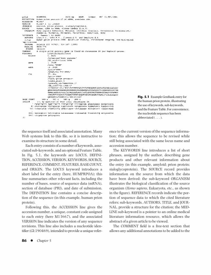
the sequence itself and associated annotation. ManyWeb systems link to this file, so it is instructive toexamine its structure in some detail.

Each entry consists of a number of keywords, asso-ciated sub-keywords, and an optional Feature Table.In Fig. 5.1, the keywords are LOCUS, DEFINI-TION, ACCESSION, VERSION, KEYWORDS, SOURCE,REFERENCE, COMMENT, FEATURES, BASE COUNT,and ORIGIN. The LOCUS keyword introduces ashort label for the entry (here, HUMPRPOA); thisline summarizes other relevant facts, including thenumber of bases, source of sequence data (mRNA),section of database (PRI), and date of submission.The DEFINITION line contains a concise descrip-tion of the sequence (in this example, human prionprotein).

Following this, the ACCESSION line gives theaccession number, a unique, constant code assignedto each entry (here M13667), and the associatedVERSION line indicates the version of any sequencerevisions. This line also includes a nucleotide iden-tifier (GI:190469), intended to provide a unique refer-

ence to the current version of the sequence informa-tion; this allows the sequence to be revised while still being associated with the same locus name andaccession number.

The KEYWORDS line introduces a list of shortphrases, assigned by the author, describing geneproducts and other relevant information about the entry (in this example, amyloid; prion protein;sialoglycoprotein). The SOURCE record providesinformation on the source from which the data have been derived; the sub-keyword ORGANISMillustrates the biological classification of the sourceorganism (Homo sapiens, Eukaryota, etc., as shownin the figure). REFERENCE records indicate the por-tion of sequence data to which the cited literaturerefers; sub-keywords, AUTHORS, TITLE, and JOUR-NAL, provide a structure for the citation; the MED-LINE sub-keyword is a pointer to an online medicalliterature information resource, which allows theabstract of a given article to be viewed.

The COMMENT field is a free-text section thatallows any additional annotations to be added to the

86 l Chapter 5

Fig. 5.1 Example GenBank entry forthe human prion protein, illustratingthe use of keywords, sub-keywords, and the Feature Table. For convenience,the nucleotide sequence has beenabbreviated ( . . . ).

BAMC05 09/03/2009 16:41 Page 86

of their contributions to dbEST in January 2004, arelisted in Table 5.2.

One of the drawbacks of the increasing levels of automation demanded by high-throughputsequencing approaches is the tendency to generateerrors. In fact, errors are a serious problem in alldatabases, not least because once they find their wayinto a resource, they tend to propagate – and themore popular the database, the more widespread thepropagation!

A notable example of the incorporation of errorsinto dbEST occurred between August 1996 andFebruary 1997, when it was discovered that up to1.5% of 892,075 ESTs submitted by WashingtonUniversity Genome Sequencing Center were mis-labeled as to species origin. More than 100 96-wellplates were found in which cDNAs from both mouseand human were present or that contained cDNAsincorrectly labeled as human or mouse. As a result,ESTs generated from these plates were tagged with a warning, and a further 657 apparently incor-rectly labeled reads from eight plates were removed

entry (here, the copy number of the gene and itschromosomal location are described). The FEA-TURES keyword marks the Feature Table, whosepurpose is to describe the properties of the sequencein detail, such as the gene name (PRNP), coordin-ates of its coding sequence (77..814), and so on.Within the Table, database cross-references aremade through the “/db_xref” qualifier (here, we seelinks to a taxonomic database (taxon:9606) and toits sequence translation in GenBank’s peptide data-base (GI:190470)). This example is not exhaustive,but indicates the type of information that can be rep-resented in the Feature Table.

The entry continues with the BASE COUNT re-cord, which details the frequency of the different basetypes in the sequence (here, 669A, 500C, 583G,668T). The ORIGIN line notes, where possible, thelocation of the first base of the sequence in the gen-ome. The nucleotide sequence itself follows, and theentry terminates with //.

5.3.5 dbEST

Expressed sequence tags (ESTs) are the product ofautomated partial DNA sequencing on randomlyselected complementary DNA (cDNA) clones. ESTsare an important research tool, as they can be usedto discover new genes, to map genes to particularchromosomes, and to identify coding regions ingenomic sequences. This fast approach to cDNAcharacterization has been particularly valuable fortagging human genes (at a fraction of the cost ofcomplete genomic sequencing) and for providingnew genetic markers.

Given their importance as a biological resourceand research tool, a significant portion of GenBankis devoted to the storage of ESTs – its EST division is termed dbEST (Boguski, Lowe, and Tolstoshev1993). In February 2004, dbEST contained morethan 20 million sequences from more than 580 different organisms; the top five organisms repres-ented in the database were H. sapiens (~5.5 mil-lion records), M. musculus (~4.0 million records), R. norvegicus (580,000 records), Triticum aestivum(500,000 records), and Ciona intestinalis (490,000records). The 20 most abundant organisms, in terms

Information resources for genes and proteins l 87

Organism No. of ESTs

Homo sapiens (human) 5,469,433Mus musculus + domesticus (mouse) 4,030,839Rattus sp. (rat) 558,402Triticum aestivum (wheat) 549,915Ciona intestinalis 492,511Gallus gallus (chicken) 451,655Danio rerio (zebrafish) 405,962Zea mays (maize) 391,145Xenopus laevis (African clawed frog) 357,038Hordeum vulgare + subsp. vulgare 348,282

(barley)Glycine max (soybean) 344,524Bos taurus (cattle) 331,139Silurana tropicalis 297,086Drosophila melanogaster (fruit fly) 267,332Oryza sativa (rice) 266,949Saccharum officinarum 246,301Sus scrofa (pig) 240,001Caenorhabditis elegans (nematode) 215,200Arabidopsis thaliana (thale cress) 196,904Medicago truncatula (barrel medic) 187,763

Table 5.2 Top 20 organisms in dbEST in January 2004.

BAMC05 09/03/2009 16:41 Page 87

completely. This was an important reminder of thepitfalls of automation, and sequence validation soft-ware was subsequently implemented to minimizethe possibility of future errors of this type.

5.3.6 DDBJ

The DNA Data Bank of Japan (Miyazaki et al. 2004)began in 1986 at the National Institute of Genetics(NIG) in Mishima. DDBJ functions as part of theINSD and receives its principal input from a varietyof sequencing centers, but especially from the inter-national human genome sequencing consortium.The database is thus growing rapidly – the numberof entries processed in 1999 alone exceeded the totalnumber processed in the preceding 10 years, and thedatabase doubled in size between July 2000 and July2001! To cope with the deluge, the curators use in-house software for mass sequence submission anddata processing, which helps both to improve con-sistency and to reduce the proliferation of errors.The Web is also used to provide standard searchtools, such as FASTA and BLAST.

In February 2004, DDBJ held 30,405,173 entries(36,079,046,032 bases). To better manage its in-creasing size, the database has been organized intospecies-oriented divisions, which facilitate moreefficient, species-specific information retrieval. Inaddition, the database includes an independent divi-sion for the patent data collected and processed bythe Japanese Patent Office, the USPTO, and the EPO.

Finally, just as translations of CDSs in EMBL are automatically added to TrEMBL, from whichcurators then create Swiss-Prot entries, so transla-tions of DDBJ are automatically added to the JapanInternational Protein Information Database ( JIPID),which in turn feeds the International PIR-PSD (seeSection 5.4).

5.3.7 The INSD

Sequence data are being generated on such a mas-sive scale that it is impossible for individual groups tocollate them. As a consequence, in February 1986,EMBL and GenBank, together with DDBJ in 1987,joined forces to streamline and standardize the pro-

cesses of data collection and annotation. Each nowcollects a portion of the total sequence data reportedworld-wide and, to achieve optimal synchronization,new and updated entries are exchanged betweenthem daily via the Internet.

The result of this tripartite collaboration is theInternational Nucleotide Sequence Database (INSD)(Fig. 5.2). This ensures that the participating data-banks share virtually the same quantity and qualityof data, and means that users need only submit toone of the resources to have their sequence reflectedin all of the others. The databases, which primarilycollect data via direct submission from individuallaboratories and large-scale sequencing projects,now incorporate DNA sequences from over 150,000different organisms, and new species are beingadded at a rate of more than 1400 per month.

As we have seen, within each of the databases, toadd value to the raw data, characteristics of thesequences are stored in Feature Tables. To improvedata consistency and reliability, and to facilitateinteroperation and data exchange, a major goal ofthe INSD was therefore to devise a common FeatureTable format and common standards for annotationpractice. The types of feature documented in thecommon format include regions that: perform par-ticular functions; affect the expression of function orthe replication of a sequence; interact with othermolecules; have secondary or tertiary structure; and so on. Regulating the content, vocabulary, andsyntax of such feature descriptions ensures that thedata are released in a form that can be exchanged

88 l Chapter 5

EMBLEBI, Europe

GenBankNCBI, USA

DDBJNIG, Japan

INSD

Fig. 5.2 The tripartite International Nucleotide SequenceDatabase (INSD), comprising EMBL (Europe), GenBank(USA), and DDBJ ( Japan).

BAMC05 09/03/2009 16:41 Page 88

In the following sections, we will briefly reviewsome of these resources and, because it is basedclosely on the structure of EMBL, we will take acloser look at the format of a typical Swiss-Protentry.

5.4.2 PIR

The Protein Sequence Database was developed at the National Biomedical Research Foundation(NBRF) in the 1960s, as mentioned above, essenti-ally as a byproduct of Dayhoff ’s studies on proteinevolution. Since 1988, the PSD has been maintainedcollaboratively by PIR-International, an associationof macromolecular sequence data collection centersthat includes PIR, JIPID, and MIPS.

More recently, PIR-PSD (Wu et al. 2003) has beenincorporated into an integrated knowledge base ofdatabases and analytical tools: this includes PIR-NREF, a comprehensive database for sequencesearching and protein identification – by Febru-ary 2004, PIR-NREF contained 1,485,025 non-redundant sequences from PIR-PSD, Swiss-Prot,TrEMBL, RefSeq, GenPept, and PDB. An interestingfeature of PIR-PSD is its emphasis on protein familyclassification, a reflection of its origins in Dayhoff’sevolutionary work. The database is thus organ-ized hierarchically around this family concept, its constituent proteins being automatically clusteredbased on sequence similarity. Within superfamilies,sequences have similar overall length and share acommon architecture (i.e., contain the same num-ber, order, and types of domain). The automatedclassification system, which places new membersinto existing superfamilies, and defines new clustersusing parameters such as sequence identity, overlaplength, and domain arrangement, is augmented bymanual annotation – this provides superfamilynames, brief descriptions, bibliographies, lists of representative and seed members, and domain andmotif architectures characteristic of the superfamily.

Linking sequences to experimentally verified datain the literature helps both to improve the qual-ity of annotation provided by the database and to avoid propagation of errors that may have re-sulted from large-scale genome-sequencing projects.

efficiently and that is readily accessible to analysissoftware.

5.4 PROTEIN SEQUENCE DATABASES

5.4.1 History

As we have seen from the above discussions, as soonas sequences began to emerge from applications ofthe earliest sequencing methods, scientists began tocollect and analyze them. In fact, the first publishedcollection of sequences was Margaret Dayhoff ’s1965 Atlas of Protein Sequence and Structure (Dayhoff1965). By 1981, the Atlas listed 1660 proteins, butthis was a “database” in paper form only, and scient-ists wishing to use the information had to type thedata into computers by hand. Burdensome thoughthis task was, two important databanks evolvedfrom this approach.

In 1984, Dayhoff ’s Atlas was released electro-nically, changing its name to the Protein Sequ-ence Database (PSD) of the Protein IdentificationResource (PIR). The first release contained 859entries; by June 2002, the collection had grownmore than 300-fold to almost 300,000 entries. Tocope with this vast expansion and ease its mainten-ance, a collaboration was formed between PIR, theMunich Information Center for Protein Sequences(MIPS), and JIPID. The resulting PIR-InternationalPSD is now one of the most comprehensive compen-dia of sequences publicly available, drawing its datafrom many sources, including sequencing centers,the literature, and directly from authors.

During this period, Amos Bairoch had begun toestablish an archive of protein sequences, initiallybased on Dayhoff ’s Atlas and later on its electronicversion. EMBL had become available in 1982, andBairoch obtained a version in 1983 containing 811sequences. His innovation was to couple the struc-tured format of EMBL entries (Section 5.3.2) withsequences from the PIR-PSD. This painstakingendeavor eventually gave rise to the first publicrelease of Swiss-Prot in 1986, which contained over 4,000 sequences; by February 2004, a 36-foldincrease in size saw that number rise to over143,790.

Information resources for genes and proteins l 89

BAMC05 09/03/2009 16:41 Page 89

Accordingly, a bibliography submission system hasbeen developed to help the scientific community tosubmit, categorize, and retrieve literature for PSDentries. This, and many other tools for databaseinterrogation, data mining and sequence analysis, isprovided via the PIR Web site.

5.4.3 MIPS

The Munich Information Center for Protein Sequ-ences (MIPS) supports national and European sequ-encing and functional analysis projects, developsand maintains genome-specific databases (e.g., forArabidopsis thaliana, Neurospora crassa, yeast), de-velops classification schemes for protein sequenceannotation, and provides tools for sequence analysis(Mewes et al. 2002). One of its central activities is tocollect and process sequence data for the tripartitePIR-International PSD.

As with PIR, a feature of the database is its auto-matic clustering of proteins into families and super-families based on sequence similarity. For familyclassification, an arbitrary cut-off of 50% identity isused – this means that resulting “families” need notnecessarily have strict biological significance. Regionsof local similarity within otherwise unrelated pro-teins are annotated as domains. Clusters (whether atfamily, superfamily, or domain level) are annotated(e.g., with protein names, EC numbers, or keywords),and are accompanied by their alignments, whichare also annotated (e.g., with domains, sequencemotifs, active sites, post-translational modifications(PTMs)). All of these resources, and a variety of ana-lysis tools, are accessible via the MIPS Web server.

5.4.4 Swiss-Prot

From its inception in 1986, Swiss-Prot was pro-duced collaboratively by the Department of MedicalBiochemistry at the University of Geneva and theEMBL. After 1994, the database transferred to theEMBL’s UK outstation, the EBI, and April 1998 sawfurther change with a move to the Swiss Institute ofBioinformatics (SIB). The database is thus nowmaintained collaboratively by the SIB and the EBI(Boeckmann et al. 2003).

Sequence information is housed in Swiss-Prot in a structured manner, adhering closely to the EMBLformat. The most important features of the resourcelie in the minimal level of redundancy it contains,the level of cross-referencing to other databases, and the quality of its annotations. In addition to the sequence itself, the annotations include biblio-graphic references and taxonomic data, and, wher-ever possible, the function of the protein, PTMs,domain structure, functional sites, associated dis-eases, similarities to other proteins, and so on. Muchof this information is gleaned from the primary lit-erature and review articles, but use is also made of a panel of experts who have particular knowledge of specific families.

A great deal of useful information about the char-acteristics of the sequence is held in the FeatureTable. This includes details of any known or pre-dicted transmembrane domains, glycosylation orphosphorylation sites, metal or ligand-binding sites,enzyme active sites, internal repeats, DNA-bindingor protein–protein interaction domains, and so on.Specially written browsers allow this information tobe viewed graphically, yielding a bird’s-eye view ofthe most important sequence features.

Swiss-Prot offers added value by providing links to over 30 different databases, including those thatstore nucleic acid or protein sequences, protein families or structures, and specialized data collec-tions. As illustrated in Fig. 5.3, it is therefore poss-ible, say, to retrieve the nucleic acid sequence(EMBL) that codes for a protein, information on associated genetic diseases (OMIM), informationspecific to the protein family to which it belongs(PROSITE, PRINTS, InterPro), and its 3D structure(PDB). Swiss-Prot thus provides a hub for data-base interconnectivity. The extent of its annotationssets Swiss-Prot apart from other protein sequenceresources and has made it the database of choice for most research purposes. By February 2004, thedatabase contained 143,790 entries.

5.4.5 The structure of Swiss-Prot entries

An example Swiss-Prot entry is shown in Fig. 5.3. As with EMBL, each line is flagged with a two-letter

90 l Chapter 5

BAMC05 09/03/2009 16:41 Page 90

Fig. 5.3 Excerpt from the Swiss-Prot entry for the human prion protein, illustrating the EMBL-like structured format, with extensive annotations and database cross-references (note: dotted lines denote points at which, for convenience, material has been excised). Compare the GenBank entry for human prion protein illustrated in Fig. 5.1. The characteristic tandem octapeptide-repeat region thought to be associated with various prion diseases has been highlighted in bold.

BAMC05 09/03/2009 16:41 Page 91

code. The first is an identification (ID) line, and thelast a // terminator. The ID codes, which attempt tobe informative and people-friendly, take the formPROTEIN_ SOURCE, where PROTEIN is an acronymthat denotes the type of protein, and SOURCEencodes the organism name. The protein in thisexample, PRIO_HUMAN, is clearly of human originand, with the eye of experience, we can deduce thatit is a prion protein.

Unfortunately, ID codes are not fixed, so an addi-tional identifier, an accession number, is also pro-vided, which should remain static between databasereleases. The accession number is provided on theAC line, here P04156, which, although meaning-less to most normal humans, is nevertheless com-puter readable (some database curators also have a disturbing capacity to be able to read accessionnumbers!). If several numbers appear on the sameAC line, the first, so-called primary accession num-ber, is the most current.

Next, the DT lines provide information about thedate of entry of the sequence to the database, anddetails of when it was last modified. The description(DE) line, or lines, then informs us of the name, ornames, by which the protein is known – here Majorprion protein precursor (PrP), PrP27-30, PrP33-35C, ASCR and CD230 antigen. The following linesgive the gene name (GN), the organism species (OS),and organism classification (OC) within the biolo-gical kingdoms.

The next part of the file provides a list of refer-ences: these can be from the literature, unpublishedinformation submitted directly from sequencing pro-jects, data from structural or mutagenesis studies,and so on. The database thus houses informationthat is difficult, or impossible, to find elsewhere. Forhuman prion protein, 30 references are provided,but for convenience, only one of these is shown inFig. 5.3.

Following the references are found comment (CC)lines. These are divided into themes describing theFUNCTION of the protein, its SUBUNIT structure,SUBCELLULAR LOCATION, DISEASE associations,and so on. Where such information is available, theCC lines also indicate any known SIMILARITY orrelationship with particular protein families. In this

example, we see that the function of the prion pro-tein is unknown, it tends to polymerize into rod-shaped fibrils, and its sequence is characterized bytandem octapeptide repeats that are believed to beassociated with various degenerative diseases.

Database cross-reference (DR) lines follow thecomment field. These provide links to other re-sources, including for example, the primary DNArepositories, protein family databases, and specialistdatabases. For human prion protein, we find links tonucleotide and protein sequence databases (EMBL,PIR), to the protein structure databank (PDB), to the online Mendelian Inheritance in Man (MIM)mutation database, and to the InterPro, PRINTS,Pfam, PROSITE, etc., family resources.

Directly after the DR lines, keywords (KW) arelisted, followed by the Feature Table (FT). The latterhighlights regions of interest in the sequence, in-cluding signal sequences, lipid attachment sites,disulfide bridges, repeats, known sequence vari-ants, and so on. Each line includes a key (e.g.,REPEAT), the location in the sequence of the feature(e.g., 51–59), and a comment, which might, forexample, indicate the level of confidence of a particu-lar annotation. For the prion example, the lipidattachment site is flagged BY SIMILARITY, indicat-ing that the assignment has been made in silicorather than in vitro and must therefore be viewed asan unverified prediction.

The final section of the file includes the sequenceitself (SQ), encoded for the sake of efficiency usingthe single-letter amino acid code. The stored sequ-ence data correspond to the precursor form of theprotein, before post-translational processing – thusinformation concerning the size or molecular weightwill not necessarily correspond to values for themature protein. The extent of mature proteins orpeptides may be deduced from the Feature Table,which indicates regions of a sequence that corres-pond to the signal (SIGNAL), transit (TRANSIT), or pro-peptide (PROPEP). The keys CHAIN and PEPTIDE are used to denote the location of themature form.

The above is not an exhaustive example, butshould provide a flavor of the richness of Swiss-Protannotations. For a more comprehensive guide to the

92 l Chapter 5

BAMC05 09/03/2009 16:41 Page 92

in Swiss-Prot – these include immunoglobulins and T-cell receptors, fragments of fewer than eightamino acids, synthetic sequences, patented se-quences, and codon translations that do not encodereal proteins.

SP-TrEMBL is partially redundant, as many of its entries are just additional reports of proteinsalready in Swiss-Prot. To reduce redundancy, andautomatically add annotation, a rule-based systemhas been designed that uses existing Swiss-Prot entries as a template. This approach can only beapplied to sequences with obvious relatives in Swiss-Prot (more sophisticated expert systems are requiredto increase the coverage by automatic annotation);nevertheless, it provides a basic level of informationthat offers a stepping-stone for further informationretrieval.

TrEMBL shares the Swiss-Prot format describedabove, and was designed to address the need for awell-structured Swiss-Prot-like resource that wouldallow rapid access to sequence data from genomeprojects, without having to compromise the qualityof Swiss-Prot itself by incorporating sequences withinsufficient analysis and annotation. A typicalTrEMBL entry is illustrated in Fig. 5.4 – comparison

type of information typically included in the data-base, and for details of the differences between theSwiss-Prot and EMBL formats, readers are referredto Appendix C of the Swiss-Prot user manual avail-able on the ExPASy Web server.

5.4.6 TrEMBL

Owing to the extent of its annotations, Swiss-Prothas become one of the most popular and widely useddatabases. However, the price paid for its manualapproach is a relatively slow rate of growth (it is lessthan half the size of PIR-PSD). Therefore, to increaseits sequence coverage, a computer-generated sup-plement was introduced in 1996, TrEMBL, based on translations of CDSs in EMBL (Boeckmann et al. 2003). In February 2004, TrEMBL contained1,075,779 entries.

TrEMBL has two main sections: (i) SP-TrEMBL(Swiss-Prot-TrEMBL), which contains entries thatwill eventually be incorporated into Swiss-Prot, but have not yet been manually annotated (theseare given Swiss-Prot accession numbers); and (ii)REM-TrEMBL (REMaining-TrEMBL), which con-tains sequences that are not destined to be included

Information resources for genes and proteins l 93

Fig. 5.4 Excerpt from the TrEMBLentry for the canine prion protein,illustrating the EMBL-like structuredformat, with automatically generatedannotations and database cross-references – there are no annotation-rich CC or FT fields (note: dotted linesdenote points at which several DR lines have been excised). Compare theSwiss-Prot entry for human prionprotein illustrated in Fig. 5.3.

BAMC05 09/03/2009 16:41 Page 93

with the (truncated) Swiss-Prot entry shown in Fig.5.3 highlights the difference in the extent of anno-tation provided by each of the resources. Note thatthere is no comment (CC) field and no Feature Table,the hallmarks of richly annotated Swiss-Prot entries.As shown, the bulk of the automatically addedannotation is largely in the form of bibliographicand database cross-references.

5.4.7 PIR-NRL3D

NRL3D (Garavelli et al. 2001) is produced by PIR-International from sequences and annotations

extracted from 3D structures deposited in the ProteinDatabank (PDB). The titles, biological sources, andkeywords of its entries have been modified from thePDB format to conform to the nomenclature stan-dards used in the other PIR databases. Bibliographicreferences and MEDLINE cross-references are in-cluded, together with secondary structure, activesite, binding site, and modified site annotations and,whenever possible, details of experimental methods,resolution, R-factor, etc.

The format of a typical PIR-NRL3D entry is illus-trated in Fig. 5.5. The example shows the sequence,together with relevant literature references and

94 l Chapter 5

Fig. 5.5 PIR-NRL3D entry for the hamster prion protein, showing the sequence, together with relevant bibliographic referencesand structural annotations. Note that the sequence is truncated by comparison with those in the GenBank, Swiss-Prot, andTrEMBL entries illustrated in Figs. 5.1, 5.3, and 5.4.

BAMC05 09/03/2009 16:41 Page 94

single record to speed searches; and the UniProtArchive (UniParc) is a comprehensive repositorythat accurately reflects the history of all proteinsequences. This unified endeavor, which bringstogether the major protein sequence data providers,is a significant achievement and should make sequ-ence analysis, for all levels of user, far easier in thefuture. UniProt is accessible via the EBI’s Web inter-face for text and similarity searches.

5.5 PROTEIN FAMILY DATABASES

5.5.1 The role of protein family databases

In addition to the numerous sequence databases,there are also many protein family databases (some-times termed pattern or secondary databases) derivedfrom the fruits of analyses of the sequences in the primary sources. Because there are several differentsources, and a variety of ways of analyzing sequ-ences, the information housed in each of the familydatabases is different – and their formats reflect thesedisparities. Although this appears to present a con-fusing picture, Swiss-Prot and TrEMBL have becomethe most popular data sources, and most familydatabases now use them as their basis. Some of themain resources are listed in Table 5.3.

From inspection of Table 5.3, it is evident that thetype of information stored in each of the familydatabases is different. Nevertheless, these resourceshave arisen from a common principle: namely, thathomologous sequences may be gathered together inmultiple alignments, within which are conserved

structural annotations from PDB entry 2PRP. Bycomparison with some of the other sequence data-bases (e.g., as shown in Figs. 5.1, 5.3, and 5.4), theextent of annotation is limited; nevertheless, it pro-vides a direct link between sequence, structure,experimental data, and the literature.

PIR-NRL3D is a valuable resource, as it makesdata in the PDB available both for keyword interro-gation and for similarity searches. Sequence infor-mation is extracted only for residues with resolved3D coordinates (as represented in PDB “ATOM”records) and not for those that are structurallyundefined. Accordingly, the sequence shown in Fig. 5.5 represents a C-terminal fragment of theprion protein, without the disordered N-terminal 90residues, which contain the characteristic octapep-tide repeat (cf. Figs. 5.1, 5.3, and 5.4).

5.4.8 UniProt

In an effort both to rationalize the currently availableprotein sequence data and to create the ultimate,comprehensive catalog of protein information, thecurators of Swiss-Prot, TrEMBL, and PIR haverecently pooled their efforts to build UniProt, theUniversal Protein Resource (Apweiler et al. 2004).UniProt comprises three components, each of whichhas been tailored for specific uses: the UniProtKnowledgebase (UniProt) is the central point ofaccess for annotated protein information (includingfunction, classification, cross-references, and so on);the UniProt Non-redundantReference (UniRef )databases combine closely related sequences into a

Information resources for genes and proteins l 95

Family database Data source Stored information

PROSITE Swiss-Prot Regular expressions (patterns)Profiles Swiss-Prot Weighted matrices (profiles)PRINTS Swiss-Prot and TrEMBL Aligned motifs (fingerprints)Pfam Swiss-Prot and TrEMBL Hidden Markov models

(HMMs)Blocks InterPro/PRINTS Aligned motifs (blocks)eMOTIF Blocks/PRINTS Permissive regular

expressions (patterns)

Table 5.3 Some of the major proteinfamily databases: in each case, the datasource is noted, together with the typeof data stored.

BAMC05 09/03/2009 16:41 Page 95

regions that show little or no variation (Fig. 5.6).Such regions, or motifs (Attwood 1997), usuallyreflect some vital biological role (i.e., are somehowcrucial to the structure or function of the protein).

Alignments have been exploited in various waysto build diagnostic signatures, or discriminators, fordifferent protein families, as illustrated in Fig. 5.6(Attwood 2000a,b, Attwood and Parry-Smith1999). An unknown query sequence may then besearched against a database of such signatures todetermine whether it contains any of the prede-fined characteristics, and hence whether it can beassigned to a particular family. As these resourcesare derived from multiple sequence information,searches of them are often better able to identify dis-tant relationships than are searches of sequencedatabases; and, if the structure and function of thefamily are known, they theoretically offer a fasttrack to the inference of biological function.However, none of these databases is complete; theyshould therefore be used to augment rather than toreplace sequence database searches. Some of themajor family databases in common use are outlinedin the following sections.

5.5.2 PROSITE

The first protein family database to have been de-veloped was PROSITE, in 1989, with 202 entries. Itis maintained collaboratively at the University ofGeneva and the Swiss Institute for ExperimentalCancer Research (ISREC) (Hulo et al. 2004). InFebruary 2004, it documented 1245 families,domains, and functional sites. The rationale behindits development was that a protein family could becharacterized by the single most conserved motifwithin a multiple alignment of its member sequ-ences, as this would likely encode a key biologicalfeature (e.g., an enzyme active site, ligand- or metal-binding site). Searching a database of such featuresshould therefore help to determine to which family a new sequence might belong, or which domain/s or functional site/s it might contain.

Within PROSITE, motifs are encoded as regularexpressions (or regexs), often referred to as patterns.Sometimes, a complete protein family cannot becharacterized by a single motif, usually because its members are too divergent. In these cases, additional regexs are designed to encode other well-

96 l Chapter 5

Single-motifmethods

Multiple-motifmethods

Fuzzy regex(eMOTIF)

Exact regex(PROSITE)

Identity matrices(PRINTS)

Weight matrices(Blocks)

Full-domainalignment methods

Profiles(Profile Library)

HMMs(Pfam)

Fig. 5.6 Illustration of the threeprincipal methods for building familydatabases, based on the use of singlemotifs, multiple motifs, and full-domainalignments.

BAMC05 09/03/2009 16:41 Page 96

example shown in Fig. 5.7, we learn that the regexwas derived from release 40.7 of Swiss-Prot, whichcontained 103,373 sequences; it matched a total of 44 sequences, all of which are true-positives – inother words, this is a good regex, with no falsematches.

The comment (CC) lines provide information onthe taxonomic range of the family (defined here aseukaryotes), and the maximum number of observedrepeats of the pattern (here just one). Following the comments are lists of the accession numbers and Swiss-Prot ID codes of all the true matches to the regex (denoted by T), and any “possible”matches (denoted by P), which are often fragments,of which there are none in this example. There areno false-positive or false-negative matches here, butwhen these do occur, they are listed after the T and P matches and are denoted by the letters F and N, respectively (the number of false and missedmatches is also documented in the NR lines).

Where structural data are available, 3D lines areused to list all relevant PDB identifiers (e.g., 1DX0,1DX1, etc.). Finally, the DO line points to the associ-ated family documentation file (here PDOC00263),and the file ends with a // terminator.

The second type of PROSITE file is the documenta-tion file, which provides details of the family (itsstructure, function, disease associations, etc.) and,

conserved parts of the alignment. When a set ofregexs is achieved that is capable of capturing all, ormost, of the characterized family from a given ver-sion of Swiss-Prot, without matching too many, orany, false positives, the results are manually anno-tated prior to deposition in PROSITE.

Entries are deposited in PROSITE in two distinctfiles. The first of these houses the regex and lists all matches in the parent version of Swiss-Prot; asshown in Fig. 5.7, the data are structured in a man-ner reminiscent of Swiss-Prot entries, where eachfield relates to a specific type of information.

Each entry contains both an identifier (ID), whichis usually some sort of acronym for the family (here,PRION_1, indicating that more than one regex hasbeen derived), and a unique accession number (AC), which takes the form PS00000. The ID linealso indicates the type of discriminator to expect in the file – the word PATTERN here tells us to expecta regular expression. A title, or description of thefamily, is contained in the DE line, and the regexitself resides on PA lines. The following NR lines provide technical details about the derivation anddiagnostic performance of the regex (for this rea-son, they are probably the most important lines toinspect when first viewing a PROSITE entry – largenumbers of false-positive and false-negative resultsare indicative of a poorly performing regex). In the

Information resources for genes and proteins l 97

Fig. 5.7 Example PROSITE entry,showing one of two data files for theprion protein family.

BAMC05 09/03/2009 16:41 Page 97

where known, a description of the biological role ofthe chosen motif/s and a supporting bibliography; asshown in Fig. 5.8, this is a free-format text file. Asevident from the figure, the structure of the docu-mentation file is much simpler than that of the datafile. Each entry is identified by its own accessionnumber (which takes the form PDOC00000), andprovides cross-references to the accession numberand identifier of its associated data file or files – in thisexample, two regexs have been derived for the fam-ily, and hence there are links to two data files

(PS00291 and PS00706). A free-format descriptionof the family and its regex(s) then follows, and the fileconcludes with relevant bibliographic references.The database is accessible for keyword and sequencesearching via the ExPASy Web server.

5.5.3 PRINTS

From inspection of sequence alignments, it is clearthat most protein families are characterized not by one, but by several conserved motifs. It therefore

98 l Chapter 5

Fig. 5.8 Example PROSITE entry, showing the documentation file for the prion protein family.

BAMC05 09/03/2009 16:41 Page 98

able. Nevertheless, overall the database is still smallrelative to the number of protein families that exist,largely because the detailed documentation ofentries is extremely time consuming. However, theextent of manually crafted annotations sets it apartfrom the growing number of automatically derivedresources, for which there is little or no biologicaldocumentation and/or result validation, and inwhich family groupings may change between data-base releases.

5.5.4 The structure of PRINTS entries

PRINTS is built as a single text file – see Fig. 5.9. Thecontents are separated into specific fields, relating togeneral information, bibliographic references, text,lists of matches, and the motifs themselves – eachline is assigned a distinct two-letter code, allowingthe database to be indexed for rapid querying(Attwood et al. 1997). Each entry begins with a 12-character identification code (an acronym thatdescribes the family – here, simply PRION), and anaccession number, which takes the form PR00000.Following this is a description of the type of entry –the term “COMPOUND” indicates that the fingerprintcontains several motifs, the number being indi-cated in parentheses (8 in this example). Details ofthe creation and latest update information are thengiven, followed by a descriptive title, and cross-refer-ences to other databases (e.g., InterPro, PROSITE,etc.), allowing users to access further informationabout the family in related resources. References arethen provided, which relate to an abstract of thefamily describing its function and structure (whereknown), its disease associations, evolutionary rela-tionships, and so on. Each abstract also contains atechnical description of how the fingerprint wasderived, including, where possible, details of thestructural and/or functional relevance of the motifs– here, the motifs encode a number of hydrophobicregions and the characteristic octapeptide repeats.

Fingerprint diagnostic performance is indicatedvia a summary that lists how many sequences madecomplete matches and how many failed to matchone or more motifs – the fewer the partial matches,the better the fingerprint (in this example, 37

makes sense to use many, or all, of these to build“fingerprints” of family membership. The techniqueof fingerprinting was first developed in 1990 – therationale behind its development was that single-motif approaches in general, and regexs in particular,are often not sufficiently powerful to characterizecertain families unambiguously. Fingerprints inher-ently offer improved diagnostic reliability overmethods of this type by virtue of the mutual contextprovided by motif neighbors: in other words, if aquery sequence fails to match all the motifs in agiven fingerprint, the pattern of matches formed bythe remaining motifs still allows the user to make areasonably confident diagnosis.

Fingerprinting was readily applicable to a diverserange of proteins, and effectively complemented theresults stored in PROSITE, especially in situationswhere particular regexs failed to provide adequatediscrimination. As a result, a prototype databasewas developed in 1990; this matured during theyears that followed, such that, in 1993, the first public release was made of a compendium of pro-tein fingerprints, containing 107 entries – this wasPRINTS (Attwood and Beck 1994). PRINTS is nowmaintained at the University of Manchester, UK,and in February 2004 contained 1850 entries(Attwood et al. 2003). The database is released inmajor and minor versions: minor releases reflectupdates, bringing the contents in line with the current version of the source database (a Swiss-Prot/TrEMBL composite); major releases denote the addition of new material to the resource. At eachmajor release, 50 new families are added to the data-base and, where necessary, old entries are updated.

Within PRINTS, motifs are encoded as ungapped,unweighted local alignments derived from an iterat-ive database-scanning procedure (the methods usedto derive fingerprints and regexs differ markedly,and are described in detail in Chapter 9). When a setof motifs is achieved that is capable of capturing all,or most, of the family from a given version of Swiss-Prot and TrEMBL, without matching too many, orany, false positives, the results are manually annot-ated prior to deposition in PRINTS.

Today, PRINTS is the most comprehensive fullymanually annotated protein family database avail-

Information resources for genes and proteins l 99

BAMC05 09/03/2009 16:41 Page 99

BAMC05 09/03/2009 16:41 Page 100

The final field relates to the motifs themselves, list-ing both the seed motifs used to generate the finger-print, followed by the final motifs (not shown) thatresult from the iterative database search procedure.Each motif is identified by its parent ID code with thenumber of that particular motif appended – for con-venience, only initial motif 1 (PRION1) is shown inFig. 5.9. After the code, the motif length is given, followed by a short description, which indicates therelevant iteration number (for the initial motifs, ofcourse, this will always be 1). The aligned motifsthemselves are then provided, together with the cor-responding source database ID code of each of theconstituent sequence fragments (here only sequ-ences from Swiss-Prot were included in the initialalignment, which contained a total of six sequ-ences). The location in the parent sequence of eachfragment is then given, together with the interval(i.e., the number of residues) between the fragmentand its preceding neighbor – for motif 1, this valueis the distance from the N terminus.

An important consequence of storing the motifs inthis “raw” form is that, unlike with regexs or other

sequences matched all eight elements of the finger-print, and one sequence matched only three motifs,indicating that this is a good fingerprint). The tablethat follows the summary breaks down this result toindicate how well individual motifs have performed,from which it is possible to deduce which motifs aremissing from any partial matches – here, we dis-cover that the reported partial hit failed to matchmotifs 2, 3, 4, 7, and 8.

After the summary are listed the ID codes of all fulland partial true- and false-positive matches, fol-lowed by their database titles. In this case, the datashow that the partial match is a chicken prion pro-tein – referring to the technical description revealsthat the reason it fails to match the fingerprint completely is that its sequence is characterized by adifferent type of tandem repeat. The scan historythen indicates which version of the source databasewas used to derive the fingerprint, and on which versions it has been updated, how many iterationswere required, what hit-list length was used, and the scanning method employed (Parry-Smith andAttwood 1992).

Information resources for genes and proteins l 101

Fig. 5.9 Example PRINTS entry, showing the fingerprint for the prion protein family. For convenience, only the first motif isdepicted. The two-letter code in the left-hand margin separates the information into specific fields (relating to text, references,motifs, etc.), which allows indexing of the data for rapid querying.

BAMC05 09/03/2009 16:41 Page 101

such abstractions, no sequence information is lost.This means that a variety of scoring methods may besuperposed onto the motifs, providing different scor-ing potentials for, and hence different perspectiveson, the same underlying data. PRINTS thus providesthe raw material for a number of automaticallyderived databases that make use of such approaches.As a consequence of being generated using moreautomated procedures, however, these resourcesprovide little or no family annotation. They there-fore further exploit PRINTS, by linking to its manually generated family documentations, whichhelp to place conserved sequence information instructural or functional contexts. This is vital for theend user, who not only wants to discover whether asequence matches a set of predefined motifs, but alsoneeds to understand their biological significance. Anumber of these, and other, automatically deriveddatabases are described in the following sections. In its original form, PRINTS is accessible for key-word and sequence searching via the University ofManchester’s Bioinformatics Web server.

5.5.5 Blocks

In 1991, the diagnostic limitations of regexs led to the creation of another multiple-motif resource, at the Fred Hutchinson Cancer Research Center(FHCRC) in Seattle – this was the Blocks database(Henikoff et al. 2000). Originally, Blocks was basedon protein families stored in PROSITE; today, how-ever, its motifs, or blocks, are created automaticallyby finding the most highly conserved regions of families held in InterPro (or by using PRINTS’ motifsdirectly – see Section 5.5.6). Different motif-detection algorithms are used and, when a con-sensus set of blocks is achieved, they are calibratedagainst Swiss-Prot to ascertain the likelihood of a chance match. Various technical details are noted,and the blocks, encoded as ungapped local align-ments, are then deposited in Blocks.

Figure 5.10 illustrates a typical block. The struc-ture of the database entry is compatible with thatused in PROSITE. An ID line provides a general codeby which the family may be identified (here Prion);this line also indicates the type of discriminator to

expect in the file – in this case, the word BLOCK tellsus to expect a block. Each block has an accessionnumber, which takes the form IPB000000X (whereIPB indicates that the block is derived from a familyin InterPro, and X is a letter that specifies which theblock is within the family’s set of blocks, e.g.,IPB000817E is the fifth prion block). The AC linealso provides an indication of the minimum andmaximum distances of the block from its precedingneighbor, or from the N terminus if it is the first in aset of blocks.

A title, or description of the family, is contained inthe DE line. This is followed by the BL line, whichprovides an indication of the diagnostic power andsome physical details of the block: these include anamino acid triplet (here CQY), which are the con-served residues used as anchors by one of the motif-detection algorithms; the width of the block and thenumber of sequences it contains; and two scores thatquantify the diagnostic power of the block – strongblocks are more effective than weak blocks (strengthless than 1100) at separating true-positives fromtrue-negatives. Following this information comesthe block itself, which indicates: the Swiss-Prot and TrEMBL IDs and accession numbers of the constituent sequences; the start position of the fragment; the sequence fragment itself; and a score,or weight, that provides a measure of the closeness ofthe relationship of that sequence to others in theblock (100 being the most distant). The file endswith a // terminator.

In February 2004, Blocks contained 4944 entriesfrom InterPro 6.0, indexed to Swiss-Prot 41.0 andTrEMBL 23.0; Blocks-format PRINTS, of course,contains the same number of entries as the versionof PRINTS from which it was derived – see Section5.5.6. Both databases are accessible for keywordand sequence searching via the Blocks Web server.

5.5.6 Blocks-format PRINTS

In addition to the Blocks database, the FHCRC Webserver provides a version of the PRINTS database inBlocks format. In this resource, the scoring methodsthat underlie the derivation of blocks have beenapplied to each of the aligned motifs in PRINTS.

102 l Chapter 5

BAMC05 09/03/2009 16:41 Page 102

Fig. 5.10 Example Blocks entry,showing the fifth block used tocharacterize the prion protein family.

BAMC05 09/03/2009 16:41 Page 103

Figure 5.11 illustrates a typical motif in Blocks format. The structure of the entry is identical to thatused in Blocks, with only minor differences occur-ring on the AC and BL lines. On the AC line, thePRINTS accession number is given, with an ap-pended letter to indicate which component of thefingerprint it is (in the example, PR00341C indic-ates that this is the third motif ). On the BL line, thetriplet information is replaced by the word “adap-ted”, indicating that the motifs have been takenfrom another resource.

Because the Blocks databases are derived auto-matically, the blocks are not annotated. Never-theless, relevant documentation may be accessedvia links to the corresponding InterPro and PRINTSentries. A further important consequence of thedirect derivation of the Blocks databases fromInterPro and PRINTS is that they offer no furtherfamily coverage. However, as different methods areused to construct the blocks in each of the databases,it is worthwhile searching both these and the parentresources.

104 l Chapter 5

Fig. 5.11 Example Blocks-formatPRINTS entry, showing the third blockused to characterize the prion proteinfamily.

BAMC05 09/03/2009 16:41 Page 104

and M fields contain position-specific profile scoresfor insert and match positions, respectively.

As in PROSITE, the pattern itself is followed by NRlines that depict the diagnostic performance of thepattern in terms of the number of true- and false-positive and false-negative results. In the example inFig. 5.12, which illustrates part of the profile entryfor WD-40 repeats, 1367 matches were made to theprofile, from a total of 352 proteins – note that thenumber of matches differs from the number of pro-teins (indicated in parentheses) because sequencesmay contain multiple copies of the WD-40 domain.Of the 1367 matches, 1362 (from 348 proteins) areknown to be true-positives; one is known to be false;25 true WD-40-containing proteins were missed;one sequence made a partial match; and for fourmatches (from three proteins) it is unknown whe-ther or not they are true family members.

Following the NR lines, a comment field (CC) pro-vides further details about the profile, such as theauthor (here K. Hofmann), the taxonomic range ofthe family, the maximum number of observedrepeats (here 15), keywords that describe the type ofmatrix (protein_domain), and so on. The familiardatabase cross-reference (DR) field then tabulatesthe database IDs and accession numbers of all true-positive (T), true-negative (N), unknown (?), andfalse-positive (F) matches to the profile in the ver-sion of Swiss-Prot indicated in the NR lines (in thiscase, 40.7).

Where structural data are available, 3D lines listall relevant PDB identifiers (e.g., 1SCG, 1A0R, etc.).Finally, the DO line points to the associated docu-mentation file (here PDOC00574), which is a textfile with identical format to that already describedfor PROSITE (Fig. 5.8). The file ends with a // terminator.

In addition to protein families and domains,profiles can be used to represent a number of othersequence features. These “special” profiles are dis-tinguished by additional information on the MAand/or CC lines. For example, MA TOPOLOGY=CIRCULAR and CC /MATRIX_TYPE=repeat_region:these lines identify a circular profile that will pro-duce one match for a repeat region consisting of several tandem repeated units. Profiles of this type

5.5.7 Profiles

An alternative philosophy to the motif-basedapproach of protein family characterization adoptsthe principle that the variable regions between con-served motifs also contain valuable information.Here, the complete sequence alignment effectivelybecomes the discriminator. The discriminator,termed a profile, is weighted to indicate where inser-tions and deletions are allowed, what types ofresidue are allowed at what positions, and where themost conserved regions are. Profiles (alternativelyknown as weight matrices) provide a sensitivemeans of detecting distant relationships, where onlyfew residues are conserved – in these circumstances,regexs cannot provide good discrimination, and willeither miss too many true-positives or will catch toomany false ones.

The limitations of regexs in identifying distanthomologs led to the creation of a compendium ofprofiles at the Swiss Institute for ExperimentalCancer Research (ISREC) in Lausanne. Each profilehas separate data and family-annotation files whoseformats are compatible with PROSITE data and documentation files. This allows results that havebeen annotated to an appropriate standard to bemade available for keyword and sequence searchingas an integral part of PROSITE via the ExPASy Webserver (Hulo et al. 2004). Those that have not yetachieved the standard of annotation necessary forinclusion in PROSITE are made available for search-ing directly via the ISREC Web server.

Figure 5.12 shows an excerpt from a profile datafile. The file structure is based on that of PROSITE,but with obvious differences. The first change is seenon the ID line, where the word MATRIX indicatesthat the type of discriminator to expect is a profile.Pattern (PA) lines are replaced by matrix (MA) lines, which list the various parameter specificationsused to derive the profile: they include details of thealphabet used (i.e., whether nucleic acid {ACGT} or amino acid {ABCDEFGHIKLMNPQRSTVWYZ});the length of the profile; cut-off scores (which aredesigned, as far as possible, to exclude randommatches); insertion and deletion penalties, insert–match–delete transition penalties; and so on. The I

Information resources for genes and proteins l 105

BAMC05 09/03/2009 16:41 Page 105

BAMC05 09/03/2009 16:41 Page 106

Information resources for genes and proteins l 107

Fig. 5.12 (opposite) Excerpt from a PROSITE profile entry, illustrating part of the profile used to characterize WD-40 repeats.

Fig. 5.13 Excerpt from a Pfam entry, illustrating some of the technical parameters stored for the prion protein family.

include: ANK_REP_REGION, for ankyrin repeats;COLLAGEN_REP, for the G–X–X collagen repeat;and PUM_REPEATS, for the pumilio RNA-bindingdomain. In addition, CC/MATRIX_TYPE=com-position denotes a profile for compositionally biasedregions, e.g., PRO_RICH, proline-rich region (suchprofiles exist for each amino acid).

5.5.8 Pfam

Just as there are different ways of using motifs tocharacterize protein families (e.g., depending on thescoring scheme used), so there are different methodsof using full sequence alignments to build family dis-criminators. An alternative to the use of profiles is toencode alignments using hidden Markov models(HMMs). These are statistically based mathematicaltreatments, consisting of linear chains of match,delete, or insert states that attempt to encode thesequence conservation within aligned families(more details in Chapter 10).

In 1994, a collection of HMMs for a range of pro-tein domains was created at the Sanger Institute – this was the Pfam database. Today, Pfam (Bateman

et al. 2004) comprises two distinct sections: (i) Pfam-A, which contains automatically generated (butoften hand-edited) seed alignments of representativefamily members, and full alignments containing all members of the family detected with an HMMconstructed from the seed alignment using theHMMER2 software; and (ii) Pfam-B, which is a fullyautomatically generated supplement derived fromthe ProDom database (Corpet et al. 2000). Full alignments in Pfam-A can be large (many containthousands of sequences) and, as with Pfam-B,because they are generated fully automatically, arenot always reliable. In February 2004, Pfam con-tained 7316 entries.

The methods that generate the best full align-ments vary for different families; the parameters aretherefore saved so that the result can be reproduced.This information, coupled with minimal annota-tions (sometimes just a descriptive family title),database and literature cross-references, etc., seedand full alignments, and the HMMs themselves,form the backbone of Pfam-A. Some of the technicaldocumentation for the prion entry is illustrated inFig. 5.13.

BAMC05 09/03/2009 16:41 Page 107

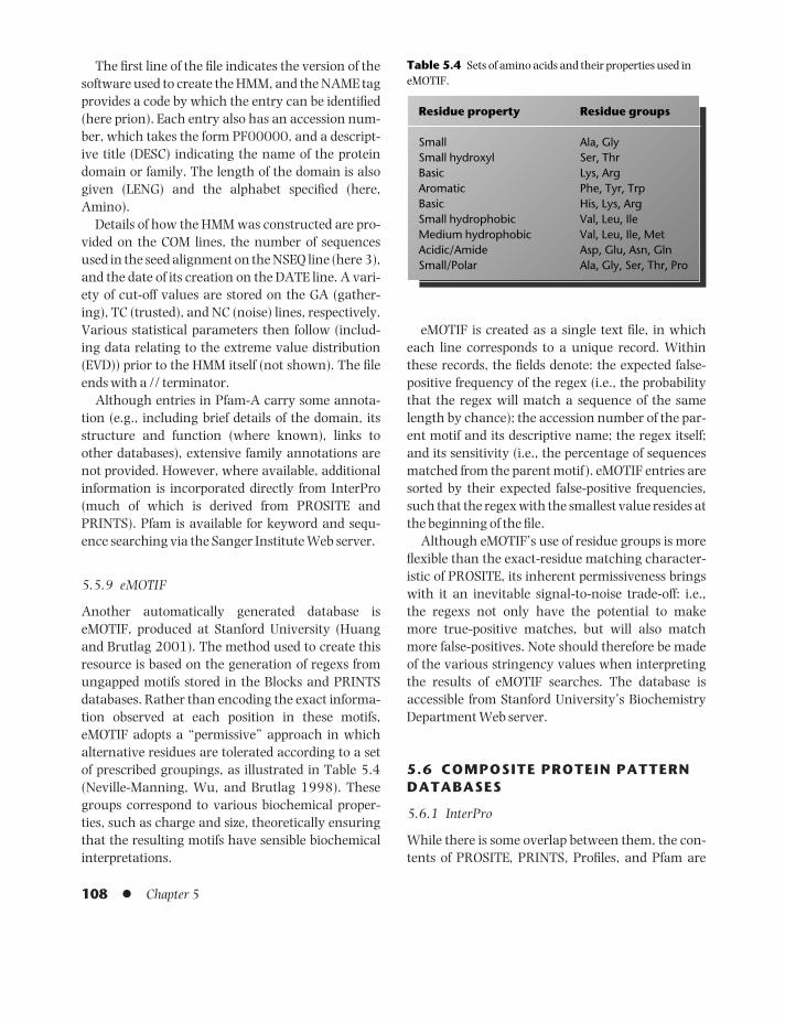
The first line of the file indicates the version of thesoftware used to create the HMM, and the NAME tagprovides a code by which the entry can be identified(here prion). Each entry also has an accession num-ber, which takes the form PF00000, and a descript-ive title (DESC) indicating the name of the proteindomain or family. The length of the domain is alsogiven (LENG) and the alphabet specified (here,Amino).

Details of how the HMM was constructed are pro-vided on the COM lines, the number of sequencesused in the seed alignment on the NSEQ line (here 3),and the date of its creation on the DATE line. A vari-ety of cut-off values are stored on the GA (gather-ing), TC (trusted), and NC (noise) lines, respectively.Various statistical parameters then follow (includ-ing data relating to the extreme value distribution(EVD)) prior to the HMM itself (not shown). The fileends with a // terminator.

Although entries in Pfam-A carry some annota-tion (e.g., including brief details of the domain, itsstructure and function (where known), links toother databases), extensive family annotations arenot provided. However, where available, additionalinformation is incorporated directly from InterPro(much of which is derived from PROSITE andPRINTS). Pfam is available for keyword and sequ-ence searching via the Sanger Institute Web server.

5.5.9 eMOTIF

Another automatically generated database iseMOTIF, produced at Stanford University (Huangand Brutlag 2001). The method used to create thisresource is based on the generation of regexs fromungapped motifs stored in the Blocks and PRINTSdatabases. Rather than encoding the exact informa-tion observed at each position in these motifs,eMOTIF adopts a “permissive” approach in whichalternative residues are tolerated according to a setof prescribed groupings, as illustrated in Table 5.4(Neville-Manning, Wu, and Brutlag 1998). Thesegroups correspond to various biochemical proper-ties, such as charge and size, theoretically ensuringthat the resulting motifs have sensible biochemicalinterpretations.

eMOTIF is created as a single text file, in whicheach line corresponds to a unique record. Withinthese records, the fields denote: the expected false-positive frequency of the regex (i.e., the probabilitythat the regex will match a sequence of the samelength by chance); the accession number of the par-ent motif and its descriptive name; the regex itself;and its sensitivity (i.e., the percentage of sequencesmatched from the parent motif ). eMOTIF entries aresorted by their expected false-positive frequencies,such that the regex with the smallest value resides atthe beginning of the file.

Although eMOTIF’s use of residue groups is moreflexible than the exact-residue matching character-istic of PROSITE, its inherent permissiveness bringswith it an inevitable signal-to-noise trade-off: i.e.,the regexs not only have the potential to make more true-positive matches, but will also matchmore false-positives. Note should therefore be madeof the various stringency values when interpretingthe results of eMOTIF searches. The database isaccessible from Stanford University’s BiochemistryDepartment Web server.

5.6 COMPOSITE PROTEIN PATTERNDATABASES

5.6.1 InterPro

While there is some overlap between them, the con-tents of PROSITE, PRINTS, Profiles, and Pfam are

108 l Chapter 5

Residue property Residue groups

Small Ala, GlySmall hydroxyl Ser, ThrBasic Lys, ArgAromatic Phe, Tyr, TrpBasic His, Lys, ArgSmall hydrophobic Val, Leu, IleMedium hydrophobic Val, Leu, Ile, MetAcidic/Amide Asp, Glu, Asn, GlnSmall/Polar Ala, Gly, Ser, Thr, Pro

Table 5.4 Sets of amino acids and their properties used ineMOTIF.

BAMC05 09/03/2009 16:41 Page 108

ated, and all method-specific annotation separatedout.

The amalgamation process is complicated by therelationships that can exist between entries in thesame database, and between entries in differentdatabases. When investigating these relationshipsmore closely, different types of parent–child rela-tionships became evident; these were subsequentlydesignated “sub-types” and “sub-strings”. A sub-string means that a motif (or motifs) is containedwithin a region of sequence encoded by a wider pat-tern (e.g., a PROSITE regex is typically containedwithin a PRINTS fingerprint, or a fingerprint mightbe contained within a Pfam domain). A sub-typemeans that one or more motifs are specific for a sub-set of sequences captured by another more generalpattern (e.g., a superfamily fingerprint may containseveral family- and subfamily-specific fingerprints;or a generic Pfam domain may include several fam-ily fingerprints). A further relationship also existsbetween InterPro entries – the “contains/found in”relationship. This arises in the case of domains thatare found in several structurally and functionallydiscrete families.

Having classified the different relationships ofcontributed entries, all recognizably distinct entitiesare assigned unique accession numbers. In doingthis, the guiding principle is that parents and chil-dren with sub-string relationships should have thesame accession numbers, while sub-type parent–child and contains/found in relationships warranttheir own accessions. In February 2004, InterProcontained 10,403 entries, including 7901 families,2239 domains, 197 repeats, 26 active sites, 20 binding sites, and 20 PTMs, built from PRINTS 37.0, PROSITE 18.1, Pfam 11.0, ProDom 2002.1,SMART 3.4, TIGRFAMs 3.0, PIR SuperFamily 2.3,and SUPERFAMILY 1.63, indexed to Swiss-Prot42.5 and TrEMBL 25.5.

5.6.2 The structure of InterPro entries

InterPro entries contain one or more signaturesfrom the individual member databases, togetherwith merged annotation and lists of matched proteins from specified versions of Swiss-Prot and

different. Furthermore, diagnostically, the resourceshave different areas of optimum application, owingto the different strengths and weaknesses of theirunderlying analysis methods: e.g., regular expres-sions are unreliable in the identification of membersof highly divergent superfamilies (where HMMs andprofiles excel); fingerprints perform relatively poorlyin the diagnosis of very short motifs (where regexs dowell); and profiles and HMMs are less likely to givespecific subfamily diagnoses (where fingerprintsexcel). Thus, while all of the resources share a common interest in protein sequence classifica-tion, some focus on divergent domains, some focuson functional sites, and others focus on families, specializing in hierarchical definitions from super-family down to subfamily levels in order to pinpointspecific functions. Therefore, in building a searchstrategy, it is sensible to include all of the availabledatabases, to ensure both that the analysis is as comprehensive as possible and that it takes advant-age of a variety of search methods.

Accessing these disparate resources, gatheringtheir different outputs, and arriving at a consensusview of the results can be quite a challenge. There-fore, in 1998, in an effort to provide a one-stop shopfor protein family diagnosis and hence make sequ-ence analysis more straightforward, the curators ofPROSITE, Profiles, PRINTS, Pfam, and ProDombegan working together to create a unified databaseof protein families. The aim was to create a singleresource, based primarily on the comprehensiveannotation in PROSITE and PRINTS, wherein eachentry would point to relevant discriminators in theparent databases – this was InterPro (Mulder et al.2003). From its first release in November 1999,InterPro proved tremendously popular, and furtherdatabases have since joined the consortium – recentadditional partners include SMART (Letunic et al.2002) and TIGRFAMs (Haft et al. 2001).

Integrating data from so many different data-bases, each of which uses different terminology andconcepts to describe families and domains, is notstraightforward. Files submitted by each of thegroups must therefore be systematically merged anddismantled before being incorporated into InterPro.Where relevant, family annotations are amalgam-

Information resources for genes and proteins l 109

BAMC05 09/03/2009 16:41 Page 109

TrEMBL. An example is shown in Fig. 5.14. Eachentry has a unique accession number (which takesthe form IPR000000), a short name, or code, bywhich the entry may be identified, and a descriptivetitle. An abstract derived from merged annotationfrom the member databases describes the family,domain, repeat or PTM, and literature referencesused to create the abstract are stored in a referencefield. Examples of representative family members arealso provided. Where relationships exist betweenentries, these are displayed in a “parent”, “child”,“contains”, or “found in” field.

Additional annotation is available for someentries in the form of mappings to Gene Ontology(GO) terms (The Gene Ontology Consortium 2001).The GO project is an effort to provide a universal sys-tem of terminology for describing gene productsacross all species. We discuss GO in Section 13.6,and consider more carefully what is meant by theword “ontology”. For the moment, we note that GOis divided into three sections describing “molecularfunction”, “biological process”, and “cellular com-ponent”. As many of these concepts are central toInterPro annotation, wherever possible its entries

110 l Chapter 5

Fig. 5.14 Excerpt from an InterPro entry, illustrating some of the annotation stored for the prion protein family.

BAMC05 09/03/2009 16:41 Page 110

keyword and sequence searching via the EBI Webserver.

5.7 PROTEIN STRUCTUREDATABASES

A discussion of the repertoire of biological databasesavailable for sequence analysis would not be completewithout some consideration of protein structure-based resources. These are limited to the relativelyfew 3D structures generated by crystallographic andspectroscopic studies, but their impact will increaseas more structures become available, notably as aresult of ongoing high-throughput structural gen-omics initiatives. In general, these resources can be divided into those that house the actual 3D coor-dinates of solved structures, and those that classifyand summarize the structures of those proteins.

5.7.1 The PDB

The PDB is the single world-wide archive of biologicalmacromolecular structures (Bourne et al. 2004). InFebruary 2004, it contained a total of 24,248 en-tries, of which 21,948 were protein, peptide, and virusstructures deduced by means of X-ray diffraction,

have been mapped to GO terms to provide an automatic means of assigning GO terms to their con-stituent proteins.

In addition to cross-referencing the member data-base signatures and GO terms, a separate field pro-vides cross-references to other databases. Includedhere are links to corresponding Blocks entries;PROSITE documentation; and the Enzyme Com-mission (EC) Database, where the EC number(s) for proteins matching the entry are shared. Whereapplicable, there may also be links to specializedresources, e.g., the CArbohydrate-Active EnZymes(CAZy) site, which describes families of related catalytic and carbohydrate-binding modules ofenzymes that act on glycosidic bonds.

A particular advantage of InterPro is that eachsequence within a family is linked to a graphical out-put that conveniently summarizes where matchesoccur to each of the signatures in the source data-bases. An example of such graphical output is illustrated in Fig. 5.15, which shows matches fromPRINTS, PROSITE, Pfam, and SMART on the humanprion sequence. This type of output also neatlyillustrates the difference between motif-based meth-ods, which match small regions of the sequence, andprofile-based methods, which more or less span the sequence completely. InterPro is available for

Information resources for genes and proteins l 111

IPR000817 PRION

IPR000817 PRION_1

IPR000817 PRION_2

IPR000817 prion

IPR000817 PRP

Fig. 5.15 Example graphical outputfrom InterPro, showing matches to thePRINTS (black), PROSITE (spotted),Pfam (striped), and SMART (checked)prion protein signatures.

Experimental Proteins, peptides, Protein/Nucleic Nucleic acids Carbohydratesmethod and viruses acid complexes

X-ray diffraction, etc. 19,014 898 719 14NMR 2,934 96 569 4Total 21,948 994 1,288 18

Table 5.5 PDB protein structure holdings in February 2004.

BAMC05 09/03/2009 16:41 Page 111

NMR, or modeling (see Table 5.5); the remainderwere nucleic acid, nucleic acid/protein complex,and carbohydrate structures.

What is not evident from these figures is that thePDB is a massively redundant resource. Owing tothe nature of research, where particular proteinsbecome the focus of repeated structure determina-tions, the contents of PDB are skewed by relativelysmall numbers of such commonly studied proteins(e.g., hemoglobin, myoglobin, lysozyme, immuno-globulins). Consequently, the number of uniquestructures within the PDB is probably little morethan 3000.

Nevertheless, the PDB is immensely valuable.Studies of protein structure archives have revealedthat many proteins share structural similarities,often reflecting common evolutionary origins, viaprocesses that involve substitutions, insertions, anddeletions in the underlying sequences. For distantlyrelated proteins, such changes can be extensive,yielding folds in which the numbers and orienta-tions of secondary structures vary considerably.However, where the functions of proteins are con-served, the structural environments of criticalactive-site residues are also generally conserved. Inan attempt to better understand sequence/structurerelationships, and the evolutionary processes thatgive rise to different fold families, a variety of struc-ture classification schemes have been established.

The nature of the information presented by struc-ture classification schemes is largely dependent onthe methods used to identify and evaluate similar-ity. Families derived, for example, using algorithms that search and cluster on the basis of commonmotifs will be different from those generated by pro-cedures based on global structure comparison; andthe results of such automatic procedures will differagain from those based on visual inspection, wheresoftware tools are used essentially to render the taskof classification more manageable. A number ofstructure-classification resources are outlined in thesections that follow.

5.7.2 SCOP

The SCOP (Structural Classification of Proteins)

database classifies proteins of known structureaccording to their evolutionary and structural rela-tionships (Andreeva et al. 2004). Domains in SCOPare grouped by species and hierarchically classifiedinto families, superfamilies, folds, and classes, a taskcomplicated by the fact that structures exhibit greatvariety, ranging from small, single domains to vastmulti-domain assemblies, so that sometimes itmakes sense to classify by individual domains, andother times at the multi-domain level. Because auto-matic structure comparison tools cannot identify allsuch relationships reliably, SCOP has been con-structed using a combination of manual inspectionand automated methods.

Proteins are classified in a hierarchical fashion toreflect their structural and evolutionary relatedness.Within the hierarchy there are many levels, butprincipally these describe the family, superfamily,and fold. The boundaries between these levels maybe subjective, but the higher levels generally reflectthe clearest structural similarities:• Families generally represent clear evolutionaryrelationships, with sequence identities greater thanor equal to 30%. This is not an absolute measure, as it is sometimes possible to infer common descentin the absence of significant sequence identity (e.g.,some members of the globin family share only 15%identity).• Superfamilies represent groups of proteins withlow sequence identity that probably share commonevolutionary origins on the basis of similar struc-tural and functional characteristics.• Folds denote major structural similarities (i.e., thesame major secondary structures in the samearrangement and with the same topology), irrespec-tive of evolutionary origin (e.g., similarities couldarise as a result of physical principles that favor par-ticular packing arrangements and fold topologies).

The seven main classes in SCOP 1.65 contain40,452 domains organized into 2327 families,1294 superfamilies, and 800 folds. These domainscorrespond to 20,619 entries in the PDB. Analyzingthe contents more closely (Table 5.6), it is clear thatthe total number of families, superfamilies, and folds(~4,400) is significantly less than the total numberof protein structures deposited in the PDB. SCOP is

112 l Chapter 5

BAMC05 09/03/2009 16:41 Page 112

homologous) – similarities are identified both bysequence- and structure-comparison algorithms.CATH is accessible for keyword interrogation via theUCL Web server.

5.7.4 PDBsum

A useful resource for accessing structural informa-tion is PDBsum (Laskowski 2001), a Web-basedcompendium of largely pictorial summaries andanalyses of all structures in the PDB. Each summarygives an at-a-glance overview of the contents of aPDB entry in terms of resolution and R factor, num-bers of protein chains, ligands, metal ions, sec-ondary structure, fold cartoons, ligand interactions,and so on. This is helpful, not only for visualizing thestructures concealed in PDB files, but also for draw-ing together information at both sequence andstructure levels. Resources of this type will becomemore and more important as visualization techni-ques improve, and new-generation software allowsmore direct interaction with their contents. InFebruary 2004, PDBsum contained 25,632 entries.The resource is accessible for keyword interrogationvia the UCL Web server.

5.8 OTHER TYPES OF BIOLOGICALDATABASE

This chapter has focused on databases of nucleic acidand protein sequences, and of protein families andprotein structures (their Web addresses are listed in

available for interrogation from the MRC Laboratoryof Molecular Biology Web server.

5.7.3 CATH

The CATH (Class, Architecture, Topology, Homology)database is a hierarchical domain classification ofprotein structures (Pearl et al. 2003). The resource islargely derived using automatic methods, but man-ual inspection is necessary where automatic meth-ods fail. Different categories within the classificationare identified by means of both unique numbers (byanalogy with the EC system for enzymes) and des-criptive names. Such a numbering scheme allowsefficient computational manipulation of the data.There are four levels within the hierarchy:• Class denotes gross secondary structure contentand packing, including domains that are: (i) mainlyα, (ii) mainly β, (iii) α − β (alternating α/β or α + βstructures), and (iv) those with low secondary struc-ture content.• Architecture describes the gross arrangement ofsecondary structures, ignoring connectivity, and isassigned manually using simple descriptions, suchas barrel, roll, sandwich, etc.• Topology assigns the overall shape and sec-ondary structure connectivity by means of structurecomparison algorithms – structures in which atleast 60% of the larger protein matches the smallerare assigned to the same level.• Homology clusters domains that share greaterthan or equal to 35% sequence identity and arethought to share a common ancestor (i.e., are

Information resources for genes and proteins l 113

Class No. of No. of No. offolds superfamilies families

All-a proteins 179 299 480All-b proteins 126 248 462a and b proteins (a/b) 121 199 542a and b proteins (a + b) 234 349 567Multi-domain proteins 38 38 53Membrane and cell surface 36 66 73

proteinsSmall proteins 66 95 150Total 800 1,294 2,327

Table 5.6 SCOP statistics for PDBrelease 1 August 2003 (excludingnucleic acids and theoretical models).

BAMC05 09/03/2009 16:41 Page 113

the Web Address Appendix at the end of this book).Beyond these is a huge variety of more specializeddatabases, with their own aims and subject coverage,and it is impossible to do justice to them all. How-ever, we will highlight two types of resource in thisnecessarily brief final section: first, species-specificdatabases, and second, databases that include infor-mation about complex biological processes andinteractions.

Many species for which genome sequencing iscomplete, or well advanced, have their own specificdatabases. Sequence information per se may not betheir primary thrust – often, the goal is to present amore integrated view of a particular biological sys-tem, in which sequence data represent just one levelof abstraction, and higher levels lead to an overallunderstanding of the genome organization. Import-ant genome databases of model organisms includeSaccharomyces cerevisiae (SGD; Dwight et al. 2002),Caenorhabditis elegans (WormBase; Stein et al. 2001),Drosophila melanogaster (FlyBase; The FlyBase Con-sortium 2002), Mus musculus (MGD; Blake et al.2003), and Arabidopsis thaliana (TAIR; Rhee et al.2003). The curators of these and other databaseshave, in recent years, worked together as the GeneOntology Consortium (see Section 13.6), whichaims to develop a consistent form of annotation forgene functions in different organisms.

There are several databases that aim to capturesome of the complexity of the processes within cells,such as metabolic pathways, and gene signaling andprotein–protein interaction networks. These types of information are fundamentally different fromsequence data and, arguably, much more complex.They thus pose challenges in terms of how to organize and store the data, and require us to think carefully about which information is import-ant to us and what we want to do with it. Importantexamples in this category are KEGG (Kanehisa et al.2002), WIT (Overbeek et al. 2000), and EcoCyc(Karp et al. 2002), UM-BBD (Ellis et al. 2001), andBIND (Bader, Betel, and Hogue 2003). Another type

of biological information results from high-through-put experimental techniques, like microarrays andproteomics. There is also an increasing awarenessthat storage and sharing of this type of experi-mental data is important, if comparisons are to be made between results from different laboratories.We discuss databases of this type specifically inSection 13.6.

Other resources of which readers should be awareinclude the Ensembl genome database (Hubbard et al. 2002), which provides a comprehensive sourceof stable automatic annotation of the humangenome sequence; UniGene (Wheeler et al. 2002),which attempts to provide a transcript map by utilizing sets of non-redundant gene-oriented clus-ters derived from GenBank sequences (the collectionrepresents genes from many organisms, includinghuman genes); TDB, which provides a substantialsuite of databases containing DNA and proteinsequence, gene expression, cellular role, and pro-tein family information, and taxonomic data formicrobes, plants, and humans (Quackenbush et al.2001); OMIM (Hamosh et al. 2002), a compendiumof genes and genetic disorders that allows systematicstudy of aspects of human disease; CDD, a com-pilation of multiple sequence alignments repres-enting protein domains conserved in molecular evolution (Marchler-Bauer et al. 2002); and hun-dreds more!

We apologize to the curators of the manydatabases we have had to leave out. As mentionedearlier, a more comprehensive overview of molecu-lar biology databases is given by Baxevanis in theannual Nucleic Acids Research (NAR) Database Issue(Baxevanis 2003) – short, searchable summariesand updates of each of the databases are availablethrough the NAR Web site. A still more compre-hensive list is available from DBcat, which enumer-ated more than 500 biological databases in 2000(Discala et al. 2000). We hope that you now feelbrave enough to go searching in today’s forest of bio-databases: happy hunting!

114 l Chapter 5

BAMC05 09/03/2009 16:41 Page 114

Attwood, T.K. 1997. Exploring the language of bioinform-atics. In H. Stanbury (ed.), Oxford Dictionary of Bio-chemistry and Molecular Biology, pp. 715–23. Oxford,UK: Oxford University Press.

Attwood, T.K. 2000a. The quest to deduce protein func-tion from sequence: The role of pattern databases. Inter-national Journal of Biochemistry Cell Biology, 32(2):139–55.

Attwood, T.K. 2000b. The role of pattern databases in sequence analysis. Briefings in Bioinformatics, 1:45–59.

REFERENCESAndreeva, A., Howorth, D., Brenner, S.E., Hubbard, T.J.P.,

Chothia, C., and Murzin, A.G. 2004. SCOP database in2004: Refinements integrate structure and sequencefamily data. Nucleic Acids Research, 32: D226–9.

Apweiler, R., Bairoch, A., Wu, C.H., Barker, W.C.,Boeckmann, B., Ferro, S., Gasteiger, E., Huang, H.,Lopez, R., Magrane, M., Martin, M.J., Natale, D.A.,O’Donovan, C., Redaschi, N., and Yeh, L.S. 2004.UniProt: the Universal Protein Knowledgebase. NucleicAcids Research, 32(1): D115–19.

Information resources for genes and proteins l 115

SUMMARY

Primary DNA sequence databases maintain complete re-cords of nucleotide sequences of all kinds, and databasedeposition of new sequences is usually a prerequisite of their publication in a scientific paper. The principalnucleotide databases are EMBL, GenBank, and DDBJ.These databases now collaborate as part of the Interna-tional Nucleotide Sequence Database (INSD), and havean agreed system of sharing information, so that sequ-ences submitted to one will automatically appear in theothers.

The most widely used primary databases of proteinsequences are PIR-PSD and Swiss-Prot. Swiss-Prot’snotoriety arises from the extent of manual annotation ofits entries. It is therefore smaller than other protein sequ-ence repositories and, for this reason, its curators devel-oped TrEMBL, an annotation-poor resource compiledautomatically from translations of coding sequences inEMBL. UniProt is an integrated resource created by theSwiss-Prot and PIR-PSD curators, providing the mostcomprehensive repository of protein sequences world-wide.

Protein family databases aim to group together pro-teins with similar sequences, structures, and functions.Proteins may be diagnosed as belonging to particularfamilies by virtue of sharing conserved sequence motifsor domains. Family databases store these diagnostic features, with annotations that relate the patterns ofconservation to known structural and functional charac-teristics. Databases of this type include PROSITE,PRINTS,and Pfam, which store regular expressions and profiles,fingerprints, and HMMs, respectively. InterPro is a col-laboration between the protein family databases that poolsthe discriminators and their annotation in an integrated

way, creating one of the most sophisticated current systems for identification and classification of proteins.

There are also databases of protein structure andstructure-based information. PDB is the principal archiveof molecular structures derived from X-ray crystallo-graphy and NMR. SCOP and CATH use these structuresto classify proteins hierarchically according to similaritiesbetween their 3D folds. Sequences and structures areprobably the most commonly used type of informa-tion in biological databases at present, but they are onlythe tip of an enormous iceberg of possibilities. A vastrange of databases now exists, capturing information onprotein–protein interactions, metabolic reaction path-ways, gene signaling networks, and information relatedto the genome projects of individual species. Integrationof these different types of biological information is now a key issue in bioinformatics.

In our discussions of databases, we emphasized theformat of their entries. A format has to be readable by both humans and computers. Although there aremany different formats, most databases have somethings in common. For example, they require a uniqueidentifier for each entry, termed an accession number,which is assigned at the time the entry is added to thedatabase and should remain static between databasereleases. Accession numbers are a quick and accurateway for computer programs to retrieve specified entries,and also provide an easy way to link entries between different databases. Most formats also contain informa-tion on the submitting authors, together with relevantscientific publications – depending on the type of infor-mation they house, some databases also include relevantannotation of sequences, their families, functions, struc-tures, and so on. This can vary from full manual annota-tion to brief automatically derived annotation.

BAMC05 09/03/2009 16:41 Page 115

Attwood, T.K., Avison, H., Beck, M.E., Bewley, M., Bleasby,A.J., Brewster, F., Cooper, P., Degtyarenko, K., Geddes,A.J., Flower, D.R., Kelly, M.P., Lott, S., Measures, K.M.,Parry-Smith, D.J., Perkins, D.N., Scordis, P., and Scott,D. 1997. The PRINTS database of protein fingerprints: Anovel information resource for computational molecu-lar biology. Journal of Chemical Information and ComputerSciences, 37: 417–24.

Attwood, T.K. and Beck, M.E. 1994. PRINTS – A proteinmotif fingerprint database. Protein Engineering, 7(7):841–8.

Attwood, T.K., Blythe, M.J., Flower, D.R., Gaulton, A.,Mabey, J.E., Maudling, N., McGregor, L., Mitchell, A.L.,Moulton, G., Paine, K., and Scordis, P. 2003. PRINTSand PRINTS-S shed light on protein ancestry. NucleicAcids Research, 30(1): 239–41.

Attwood, T.K. and Parry-Smith, D.J. 1999. Introduction toBioinformatics. Harlow, UK: Addison Wesley Longman.

Bader, G.D., Betel, D., and Hogue, C.W.V. 2003. BIND: The Biomolecular Interaction Database. Nucleic AcidsResearch, 31: 248–50.

Bateman, A., Coin, L., Durbin, R., Finn, R.D., Hollich, V.,Griffiths-Jones, S., Khanna, A., Marshall, M., Moxon, S.,Sonnhammer, E.L.L., Studholme, D.J., Yeats, C., andEddy, S.R. 2004. The Pfam protein families database.Nucleic Acids Research, 32: D138–44.

Baxevanis, A.D. 2003. The Molecular Biology DatabaseCollection: 2003 update. Nucleic Acids Research, 31:1–12.

Benson, D.A., Karsch-Mizrachi, I., Lipman, D.J., Ostell, J.,and Wheeler, D.L. 2004. GenBank: Update. NucleicAcids Research, 32: D23–6.

Boeckmann, B., Bairoch, A., Apweiler, R., Blatter, M.C.,Estreicher, A., Gasteiger, E., Martin, M.J., Michoud, K.,O’Donovan, C., Phan, I., Pilbout, S., and Schneider, M.2003. The Swiss-Prot protein knowledge base and itssupplement TrEMBL in 2003. Nucleic Acids Research,31(1): 365–70.

Boguski, M.S., Lowe, T.M., and Tolstoshev, C.M. 1993.dbEST – database for “expressed sequence tags”. NatureGenetics, 4(4): 332–3.

Blake, J.A., Richardson, J.E., Bult, C.J., Kadin, J.A., Eppig,J.T., and the Mouse Genome Database Group. 2003.MGD: The Mouse Genome Database. Nucleic AcidsResearch, 31: 193–5.

Bourne, P.E., Addess, K.J., Bluhm, W.F., Chen, L.,Deshpande, N., Feng, Z., Fleri, W., Green, R., Merino-Ott,J.C., Townsend-Merino, W., Weissig, H., Westbrook, J.,and Berman, H.M. 2004. The distribution and query

systems of the RCSB Protein Data Bank. Nucleic AcidsResearch, 32: D223–5.

Corpet, F., Servant, F., Gouzy, J., and Kahn, D. 2000.ProDom and ProDom-CG: Tools for protein domainanalysis and whole genome comparisons. Nucleic AcidsResearch, 28(1): 267–9.

Dayhoff, M.O. 1965. Atlas of Protein Sequence and Structure.Silver Spring, MD: National Biomedical ResearchFoundation.

Discala, C., Benigni, X., Barillot, E., and Vaysseix, G. 2000.DBCat: A catalog of 500 biological databases. NucleicAcids Research, 28(1): 8–9.

Dwight, S.S., Harris, M.A., Dolinski, K., Ball, C.A., Binkley,G., Christie, K.R., Fisk, D.G., Issel-Tarver, L., Schroeder,M., Sherlock, G., Sethuraman, A., Weng, S., Botstein,D., and Cherry, M.J. 2002. Saccharomyces GenomeDatabase (SGD) provides secondary gene annotationusing the Gene Ontology (GO). Nucleic Acids Research,30(1): 69–72.

Ellis, L.B.M., Hershberger, C.D., Bryan, E.M., and Wackett,L.P. 2001. The University of Minnesota Biocatalysis/Biodegradation Database: Emphasizing enzymes. NucleicAcids Research, 29(1): 340–3.

Etzold, T., Ulyanov, A., and Argos, P. 1996. SRS –Information-retrieval system for molecular-biology data-banks. Methods in Enzymology, 266: 114–28.

Garavelli, J.S., Hou, Z., Pattabiraman, N., and Stephens,R.M. 2001. The RESID Database of protein structuremodifications and the NRL-3D Sequence–StructureDatabase. Nucleic Acids Research, 29(1): 199–201.

Haft, D.H., Loftus, B.J., Richardson, D.L., Yang, F., Eisen,J.A., Paulsen, I.T., and White, O. 2001. TIGRFAMs: Aprotein family resource for the functional identificationof proteins. Nucleic Acids Research, 29(1): 41–3.

Hamosh, A., Scott, A.F., Amberger, J., Bocchini, C., Valle,D., and McKusick, V.A. 2002. Online Mendelian Inher-itance in Man (OMIM), a knowledge base of humangenes and genetic disorders. Nucleic Acids Research,30(1): 52–5.

Henikoff, J.G., Greene, E.A., Pietrokovski, S., and Henikoff,S. 2000. Increased coverage of protein families with theBlocks database servers. Nucleic Acids Research, 28(1):228–30.

Huang, J.Y. and Brutlag, D.L. 2001. The eMOTIF data-base. Nucleic Acids Research, 29(1): 202–4.

Hubbard, T., Barker, D., Birney, E., Cameron, G., Chen, Y.,Clark, L., Cox, T., Cuff, J., Curwen, V., Down, T., Durbin,R., Eyras, E., Gilbert, J., Hammond, M., Huminiecki, L.,Kasprzyk, A., Lehvaslaiho, H., Lijnzaad, P., Melsopp, C.,

116 l Chapter 5

BAMC05 09/03/2009 16:41 Page 116

Bucher, P., Copley, R.R., Courcelle, E., Das, U., Durbin,R., Falquet, L., Fleischmann, W., Griffith-Jones, S., Haft,D., Harte, N., Hermjakob, H., Hulo, N., Kahn, D.,Kanapin, A., Krestyaninova, M., Lopez, R., Letunic, I.,Lonsdale, D., Silventoinen, V., Orchard, S., Pagni, M.,Peyruc, D., Ponting, C.P., Servant, F., Sigrist, C.J.A.,Vaughan, R., and Zdobnov, E. 2003. The InterProdatabase – 2003 brings increased coverage and newfeatures. Nucleic Acids Research, 31(1): 315–18.

Neville-Manning, C.G., Wu, T.D., and Brutlag, D.L. 1998.Highly specific protein sequence motifs for genome ana-lysis. Proceedings of the National Academy of Sciences USA,95: 5865–71.

Overbeek, R., Larsen, N., Pusch, G.D., D’Souza, M., Selkov,E., Jr., Kyrpides, N., Fonstein, M., Maltsev, N., andSelkov, E. 2000. WIT: Integrated system for high-throughput genome sequence analysis and metabolicreconstruction. Nucleic Acids Research, 28(1): 123–5.

Parry-Smith, D.J. and Attwood, T.K. 1992. ADSP – A newpackage for computational sequence analysis. CABIOS,8(5): 451–9.

Pearl, F.M.G., Bennett, C.F., Bray, J.E., Harrison, A.P.,Martin, N., Shepherd, A., Sillitoe, I., Thornton, J., andOrengo, C.A. 2003. The CATH database: An extendedprotein family resource for structural and functionalgenomics. Nucleic Acids Research, 31: 452–5.

Quackenbush, J., Cho, J., Lee, D., Liang, F., Holt, I.,Karamycheva, S., Parvizi, B., Pertea, G., Sultana, R.,and White, J. 2001. The TIGR Gene Indices: Analysis ofgene transcript sequences in highly sampled eukaryoticspecies. Nucleic Acids Research, 29(1): 159–64.

Rhee, S.Y. et al. 2003. The Arabidopsis InformationResource (TAIR): A model organism database providinga centralized, curated gateway to Arabidopsis biology, re-search materials and community. Nucleic Acids Research,31: 224–8.

Stein, L., Sternberg, P., Durbin, R., Thierry-Mieg, J., andSpieth, J. 2001. WormBase: Network access to thegenome and biology of Caenorhabditis elegans. NucleicAcids Research, 29(1): 82–6.

Schuler, G.D. 1996. Entrez: Molecular biology databaseand retrieval system. Methods in Enzymology, 266: 141–62.

The FlyBase Consortium. 2002. The FlyBase database ofthe Drosophila genome projects and community liter-ature. Nucleic Acids Research, 30(1): 106–8.

The Gene Ontology Consortium. 2001. Creating the geneontology resource: Design and implementation. GenomeResearch, 11: 1425–33.

Mongin, E., Pettett, R., Pocock, M., Potter, S., Rust, A.,Schmidt, E., Searle, S., Slater, G., Smith, J., Spooner, W.,Stabenau, A., Stalker, J., Stupka, E., Ureta-Vidal, A.,Vastrik, I., and Clamp, M. 2002. The Ensembl genomedatabase project. Nucleic Acids Research, 30(1): 38–41.

Hulo, N., Sigrist, C.J., Le Saux, V., Langendijk-Genevaux,P.S., Bordoli, L., Gattiker, A., De Castro, E., Bucher, P.,and Bairoch, A. 2004. Recent improvements to thePROSITE database. Nucleic Acids Research, 32(1):D134–7.

Kanehisa, M., Goto, S., Kawashima, S., and Nakaya, A.2002. The KEGG databases at GenomeNet. Nucleic AcidsResearch, 30(1): 42–6.

Karp, P.D., Riley, M., Saier, M., Paulsen, I.T., Collado-Vides, J., Paley, S.M., Pellegrini-Toole, A., Bonavides, C.,and Gama-Castro, S. 2002. The EcoCyc Database.Nucleic Acids Research, 30(1): 56–8.

Kulikova, T., Aldebert, P., Althorpe, N., Baker, W., Bates,K., Browne, P., van den Broek, A., Cochrane, G.,Duggan, K., Eberhardt, R., Faruque, N., Garcia-Pastor,M., Harte, N., Kanz, C., Leinonen, R., Lin, Q., Lombard,V., Lopez, R., Mancuso, R., McHale, M., Nardone, F.,Silventoinen, V., Stoehr, P., Stoesser, G., Tuli, M.A.,Tzouvara, K., Vaughan, R., Wu, D., Zhu, W., andApweiler, R. 2004. The EMBL Nucleotide SequenceDatabase. Nucleic Acids Research, 32: D27–30.

Laskowski, R.A. 2001. PDBsum: Summaries and ana-lyses of PDB structures. Nucleic Acids Research, 29(1):221–2.

Letunic, I., Goodstadt, L., Dickens, N.J., Doerks, T., Schultz,J., Mott, R., Ciccarelli, F., Copley, R.J., Ponting, C.P., andBork, P. 2002. Recent improvements to the SMARTdomain-based sequence annotation resource. NucleicAcids Research, 30(1): 242–4.

Marchler-Bauer, A., Panchenko, A.R., Shoemaker, B.A.,Thiessen, P.A., Geer, L.Y., and Bryant, S.H. 2002. CDD:A database of conserved domain alignments with linksto domain three-dimensional structure. Nucleic AcidsResearch, 30(1): 281–3.

Mewes, H.W., Frishman, D., Güldener, U., Mannhaupt, G.,Mayer, K., Mokrejs, M., Morgenstern, B., Münsterkötter,M., Rudd, S., and Weil, B. 2002. MIPS: A database forgenomes and protein sequences. Nucleic Acids Research,30(1): 31–4.

Miyazaki, S., Sugawara, H., Gojobori, T., and Tateno, Y.2004. DDBJ in the stream of various biological data.Nucleic Acids Research, 32: D31–4.

Mulder, N.J., Apweiler, R., Attwood, T.K., Bairoch, A.,Bateman, A., Binns, D., Biswas, M., Bradley, P., Bork, P.,

Information resources for genes and proteins l 117

BAMC05 09/03/2009 16:41 Page 117

Wheeler, D.L., Church, D.M., Lash, A.E., Leipe, D.D.,Madden, T.L., Pontius, J.U., Schuler, G.D., Schriml,L.M., Tatusova, T.A., Wagner, L., and Rapp, B.A. 2002.Database resources of the National Center for Biotech-nology Information: 2002 update. Nucleic Acids Research,30(1): 13–16.

Wu, C.H., Yeh, L-S.L., Huang, H., Arminski, L., Castro-Alvear, J., Chen, Y., Hu, Z.Z., Ledley, R.S., Kourtesis, P.,Suzek, B.E., Vinayaka, C.R., Zhang, J., and Barker, W.C.2003. The Protein Information Resource. Nucleic AcidsResearch, 31(1): 345–7.

118 l Chapter 5

BAMC05 09/03/2009 16:41 Page 118

Sequence alignmentalgorithms

As a simple example, sup-pose we have a list of numbersin a random order and wewish to sort them into ascend-ing order (see Fig. 6.1(a)).One easy algorithm for doingthis is called Insertion Sort,which can be described in thefollowing way:

• If the second element is less than the first element,move the second element one place to the left (in thiscase, swap 22 with 71).• If the third element is less than the second, movethe third element to the left. If this element is also lessthan the first element, move it another place to theleft (in this case, 9 moves to the beginning of the list).• Consider each subsequent element and move it tothe left until the element preceding it is lower than itor until it reaches the beginning of the list (e.g., 18 ismoved to second position).• Continue until all elements are in ascending order.It would be easy to write a computer program tocarry out this algorithm. You could also do it your-self by hand (e.g., if you were sorting a pack of play-ing cards into ascending numerical value).

An important property of algorithms is how longthey take to carry out or, more specifically, how thetime taken scales with the size of the problem, N. In this example, N is the number of elements in thelist to be sorted. Since there are N elements to move,the time taken must at least be proportional to N.However, each element must be compared with several elements to its left in order to slide it into its

Sequence alignment algorithms l 119

CHAPTER

6

6.1 WHAT IS AN ALGORITHM?

The sequence alignment problem is fundamental tobioinformatics. Alignments show us which bits of asequence are variable and which bits are conserved.They indicate the positions of insertions and dele-tions. They allow us to identify important functionalmotifs. They are the starting point for evolutionarystudies using phylogenetic methods. They form thebasis of database search methods. You can’t get farin gene sequence analysis without an alignment.Before describing the computational methods usedto produce alignments, we need to explain what ismeant by the term algorithm.

An algorithm is a series of instructions that explainhow to solve a particular problem. It is a recipe thatdescribes what steps to take to obtain the desiredanswer. It consists of a series of logical or mathemat-ical statements that explain what to do in what cir-cumstances. An algorithm is not itself a computerprogram, but a good programmer should easily beable to translate any properly defined algorithm intoa program in any programming language.

CHAPTER PREVIEWWe present the dynamic programming algorithms used for pairwise sequencealignment. We consider variations in the algorithm that account for differenttypes of gap cost functions and for global and local alignments. Examples aregiven that show the sensitivity of the results to the scoring parameters used. Wethen discuss heuristic algorithms for multiple sequence alignment, focusing onthe commonly used progressive alignment technique.

BAMC06 09/03/2009 16:40 Page 119

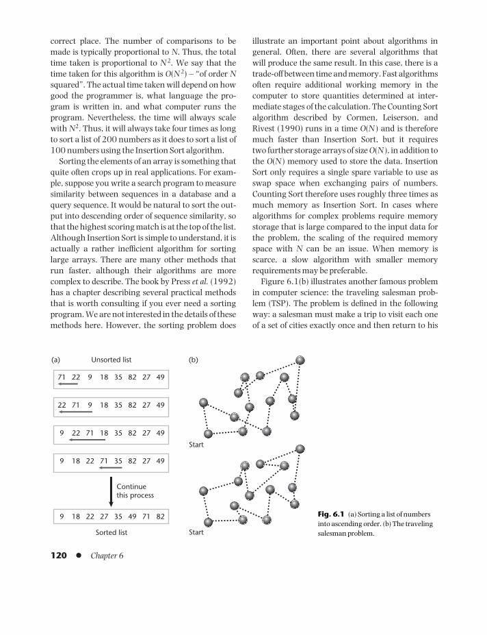
correct place. The number of comparisons to bemade is typically proportional to N. Thus, the totaltime taken is proportional to N 2. We say that thetime taken for this algorithm is O(N 2) – “of order Nsquared”. The actual time taken will depend on howgood the programmer is, what language the pro-gram is written in, and what computer runs the program. Nevertheless, the time will always scalewith N2. Thus, it will always take four times as longto sort a list of 200 numbers as it does to sort a list of100 numbers using the Insertion Sort algorithm.

Sorting the elements of an array is something thatquite often crops up in real applications. For exam-ple, suppose you write a search program to measuresimilarity between sequences in a database and aquery sequence. It would be natural to sort the out-put into descending order of sequence similarity, sothat the highest scoring match is at the top of the list.Although Insertion Sort is simple to understand, it isactually a rather inefficient algorithm for sortinglarge arrays. There are many other methods thatrun faster, although their algorithms are more complex to describe. The book by Press et al. (1992)has a chapter describing several practical methodsthat is worth consulting if you ever need a sortingprogram. We are not interested in the details of thesemethods here. However, the sorting problem does

illustrate an important point about algorithms ingeneral. Often, there are several algorithms that will produce the same result. In this case, there is atrade-off between time and memory. Fast algorithmsoften require additional working memory in thecomputer to store quantities determined at inter-mediate stages of the calculation. The Counting Sortalgorithm described by Cormen, Leiserson, andRivest (1990) runs in a time O(N ) and is thereforemuch faster than Insertion Sort, but it requires two further storage arrays of size O(N ), in addition tothe O(N ) memory used to store the data. InsertionSort only requires a single spare variable to use asswap space when exchanging pairs of numbers.Counting Sort therefore uses roughly three times asmuch memory as Insertion Sort. In cases wherealgorithms for complex problems require memorystorage that is large compared to the input data forthe problem, the scaling of the required memoryspace with N can be an issue. When memory isscarce, a slow algorithm with smaller memoryrequirements may be preferable.

Figure 6.1(b) illustrates another famous problemin computer science: the traveling salesman prob-lem (TSP). The problem is defined in the followingway: a salesman must make a trip to visit each one of a set of cities exactly once and then return to his

120 l Chapter 6

(a) (b)

Start

Start

Unsorted list

Sorted list

71 22 9 18 35 82 27 49

22 71 9 18 35 82 27 49

9 22 71 18 35 82 27 49

9 18 22 71 35 82 27 49

9 18 22 27 35 49 71 82

Continuethis process

Fig. 6.1 (a) Sorting a list of numbersinto ascending order. (b) The travelingsalesman problem.

BAMC06 09/03/2009 16:40 Page 120

starting point. The distance between each pair ofcities is specified in advance. The problem is to findthe route that minimizes the total distance traveled.The upper figure shows one rather long route thatwastes time by crossing over itself in several places.The lower figure shows a more plausible route thatprobably does not go too much farther than neces-sary; however, it may not be the best. If there are Ncities, then there are N! possible routes. One way ofsolving the TSP that is guaranteed to give the bestanswer is by exact enumeration, i.e., a computercould be asked to consider every one of the possibleorders in turn and save the best one. The timerequired would also increase as N!, which is huge(see Section M.2). So exact enumeration would onlybe possible for very small N.

There are many computational problems wherethe number of cases to be considered increases eitherfactorially (as N!) or exponentially (as αN for someconstant α). In both cases, exact enumeration of allthe cases becomes impossible for large values of N.Nevertheless, there are often algorithms that cansolve the problem in “polynomial time”, i.e., in atime that is O(N β), for some constant β. The bestalgorithms have β as small as possible. For example, in the sorting problem there are also N! possibleorderings of the N elements, but we do not need tocheck all these orderings one by one. The InsertionSort method is a polynomial time algorithm with β = 2. On the other hand, the TSP is an example of a problem for which there is no known algorithmthat can solve the problem exactly in polynomialtime. Computationally difficult problems like this are known as NP-complete (where NP stands fornondeterministic polynomial – see Cormen et al.1992). Where we cannot find exact algorithms thatare guaranteed to give the correct answer, heuristicalgorithms are used. A heuristic algorithm is onethat we believe is likely to give a fairly good solutionmost of the time, even though we cannot prove thatthe solution given is really the best one.

One possible heuristic algorithm for the TSPwould simply be always to travel to the nearest citythat you have not been to before. This is likely to pro-duce a route that is not too bad – certainly it will bemuch better than a random route. However, it may

lead to a situation where the last city visited is veryfar from the starting point, and hence there will be avery large distance to travel home. This type ofheuristic is known as a greedy algorithm. Greedyalgorithms are shortsighted, i.e., they always dowhat is best in the short term. Often, greedy algo-rithms can be proposed as first solutions to a prob-lem, and can then be improved by better heuristicalgorithms. There is a large literature on the devel-opment of heuristic algorithms for the TSP. Bothexact and heuristic algorithms will arise in our discussion of alignment methods in this chapter. Inmolecular phylogenetics, we also require heuristicalgorithms to search through very large numbers ofpossible evolutionary trees (see Section 8.5).

6.2 PAIRWISE SEQUENCEALIGNMENT – THE PROBLEM

We will begin with the basic problem of aligning twosequences. A pairwise alignment of two DNA sequ-ences looks something like this:

CAGT-AGATATTTACGGCAGTATC----

CAATCAGGATTTT--GGCAGACTGGTTG

Gaps have been inserted in both the top and the bottom sequence in order to slide the sequencesalong so that the regions of similarity between themare apparent. When we align two sequences, weusually do so because they are homologous, i.e., webelieve they have evolved from a common ancestor.The alignment above means that the first two sitesCA have remained unchanged, while there has beena mutation at the third site from a G to an A or froman A to a G (we don’t know which). The gap at thefifth site means that either there has been a deletionin the top sequence or there has been an insertion ofa C in the bottom sequence (again we don’t knowwhich). When we look for the “best” alignment oftwo sequences, we are really looking for the align-ment that we think is most likely to have occurredduring evolution.

In order to obtain the best alignment, we need ascoring system. We know that the sequences to be

Sequence alignment algorithms l 121

BAMC06 09/03/2009 16:40 Page 121

aligned are composed of letters from an alphabet ofallowed characters. For DNA, the alphabet is just A,C, G, and T. For proteins, it is the 20-letter alphabetcorresponding to the amino acids. The first part ofthe scoring system is to define a score, S(α,β), forevery pair of letters in the allowed alphabet. ForDNA, the scoring system is usually a very simpleone: we assign S(α,β) = 1 whenever α and β are thesame nucleotide, and S(α,β) = 0 whenever they aredifferent nucleotides. For proteins, we could alsoassign 1 for identical amino acids and 0 for differentamino acids if we wished; however, this is not a veryuseful scoring system for proteins in practice. A goodscoring system needs to reflect the fact that someamino acids are similar to one another and some aredifferent. We want to assign a high positive score totwo identical amino acids, a slightly positive score totwo similar amino acids (say, D and E, or I and L),and a slightly negative score for two amino acidsthat are very different from one another (say, D andI). In Chapter 4, we discussed the way scoring matrices, such as PAM and BLOSUM, are calculated.Any matrix of scores like this offers a possible scoringsystem for aligning protein sequences. The align-ment algorithm works in the same way whateverscores we use, but the optimal alignment producedby the algorithm will depend on the scoring system.

The second part of the scoring system is thepenalty for gaps. In general, let us define W(l) as thepenalty for a gap of length l characters. The simplestfunction we can choose is a linear gap penalty: W(l)= gl. This mean that each individual gap characterhas a cost g, and the cost of the full gap is just g timesthe length. However, in reality, it may not be that agap of three residues is three times as unlikely as agap of a single residue. It could be that a single eventcreated a gap of three residues. The likelihood of thisoccurring therefore depends on the underlyingmutational process, i.e., the error in DNA replicationthat created the gap in this gene. It also depends onthe selection process. We will usually be aligningsequences that are real working molecules. Manyinsertions or deletions may lead to molecules thatare nonfunctional (e.g., frame-shift mutations in thecoding regions of DNA) and those sequences will beeliminated by selection. There are certain regions of

sequences where we tend to find gaps and certainregions where we don’t. For example, unstructured“loop” regions in proteins tend to be much morevariable than regions with well-defined structures,such as helices in membrane proteins. Taking allthese effects into account, we might expect that thecost function W(l) should look something like thecurve in Fig. 6.2. It should increase steeply at first,because making a gap is an unlikely evolutionaryevent, but then it should increase less steeply as l getslarger, because if we already know that a gap is pos-sible at this position, then it may not be much moreunlikely to have a bigger gap than a smaller one.

There is no real theory to tell us what function touse for gap penalties, although some progress hasbeen made in analyzing the empirical distribution of gap sizes (Benner, Cohen, and Gonnet 1993). For practical reasons, the gap-scoring system is usually kept fairly simple. The most widely used gap-scoring system in real applications is the AffineGap Penalty function. Here, we suppose that thepenalty for opening a new gap is gopen, and thepenalty for extending the gap for each subsequentstep is gext. Hence the penalty for a gap of length l isW(l) = gopen + gext(l − 1). This is shown as the dashedline in Fig. 6.2. Usually gext < gopen for the reasons

122 l Chapter 6

0 1 2Gap length (l)

3 4 5

Gap

cos

t

W(l) = gl

W(l) = gopen + gext(l –1)General gap cost W(l)

Fig. 6.2 Gap cost functions W(l) – linear, affine, and generalgap functions are shown.

BAMC06 09/03/2009 16:40 Page 122

given above. In fact, the Affine Gap Penalty functionis not that far from the general curved shape that we might expect. An extreme case would be to setgext = 0, in which case the penalty of a gap would bejust gopen, independent of its length.

Having defined our scoring system, it is possible tocalculate a score for any pairwise alignment, such asthe one at the beginning of this section:

(6.1)

The principle of pairwise alignment algorithms isthat we consider every possible way of aligning twosequences by sliding one with respect to the otherand inserting gaps in both sequences, and we determine the alignment that has the highest score.The number of alignments is huge (it increases fac-torially with the lengths of the sequences), hence wecannot simply enumerate all possible alignments.However, polynomial time algorithms are knownfor solving this problem using a method known asdynamic programming.

6.3 PAIRWISE SEQUENCEALIGNMENT – DYNAMICPROGRAMMING METHODS

6.3.1 Algorithm 1 – Global alignment with linear gap penalty

Suppose we have two sequences with lengths N1 andN2. The letters in the first sequence will be denoted ai(where 1 ≤ i ≤ N1) and the letters in the secondsequence will be denoted bj (where 1 ≤ j ≤ N2). Wewill define H(i, j) as the score of the best alignmentthat can be made using the first i letters of the firstsequence and the first j letters of the second sequ-ence. We want to calculate the score H(N1,N2) foraligning the full sequences. To do this, we will haveto calculate H(i, j) for each value of i and j and gra-dually build up to the full length.

The first algorithm we consider is known as theNeedleman–Wunsch algorithm after its originators(Needleman and Wunsch 1970). We wish to calcu-late H(i, j), the score for the partial alignment ending

Score S W laligned

pairsgaps

( , ) ( )= −∑ ∑α β

in ai and bj. There are only three things that can hap-pen at the end of this partial alignment: (i) ai and bjare aligned with each other; (ii) ai is aligned with agap; or (iii) bj is aligned with a gap. Since we want thehighest alignment score, H(i, j) is the maximum ofthe scores corresponding to these three possibilities.Hence we may write

(6.2)

In option (i), we add the score S(ai,bj) for aligningai and bj to the score H(i − 1, j − 1) for aligning thesequences up to ai −1 and bj −1. In option (ii), we havecreated a gap; therefore, we pay a cost, g, which wesubtract from the score H(i − 1, j) for aligning thesequences up to ai−1 and bj. Similarly, in option (iii),we subtract g from the score for aligning the sequ-ences up to ai and bj−1.

The scores H(i, j) are the elements of a matrix wherei labels the rows and j labels the columns. Option (i) corresponds to making a diagonal step from the topleft of the matrix towards the bottom right. Option(ii) corresponds to making a step vertically down-wards, and option (iii) corresponds to making a stephorizontally from left to right. Equation (6.2) saysthat if we want to know the score for the cell (i, j) inthe matrix, then we need to know the score for thediagonal, vertical, and horizontal neighbors of thiscell. The key point about Eq. (6.2) is that it works forevery value of i and j. We can use the same formulato work out the scores for the three neighbors interms of their neighbors. This formula is called arecursion relation. We can use it recursively for eachcell in the matrix, starting with small values of i and jand building up to large ones.

In order to get started with this recursion, we needto know some initial conditions. In this case, weknow that H(i,0) = −gi. This means that the first iletters of sequence 1 are aligned with nothing at allfrom sequence 2. Hence there is a gap of size i at thebeginning, which costs −gi. Similarly, H(0, j) = −gj,which corresponds to the first j letters of sequence 2

H i jH i j S a b

H i j gH i j g

i j

( , ) max( , ) ( , )

( , ) ( , )

=− − +

− −− −

⎧⎨⎪

⎩⎪

1 11

1

diagonalvertical

horizontal

Sequence alignment algorithms l 123

BAMC06 09/03/2009 16:40 Page 123

being aligned with nothing in sequence 1. It is alsonecessary to define H(0,0) = 0. This means that thescore is 0 before we begin the alignment.

As an example, we will align the two proteinsequences SHAKE and SPEARE using the PAM250scoring matrix that was already shown in Fig. 4.6.From this, we may calculate a score S(ai,bj) for eachpair of amino acids that occur in this example. Forconvenience, these scores are shown in Fig. 6.3(a).We now draw out the matrix H(i, j), as in Fig. 6.3(b),including a row and column corresponding to i = 0and j = 0. Initially, all the numbers in the cells are unknown; however, we can start right away byfilling in the cells corresponding to the initial con-ditions. Let the gap cost be g = 6. All the cells aroundthe edge of the matrix will have scores that are multiples of −6. For example, H(3,0) = −18, andH(0,2) = −12. These correspond to the two partialalignments

SHA and --

--- SP

We can now proceed with the row i = 1. From Eq.(6.2), the options for cell (1,1) are

S(0+2=2) or -S(-6-6=-12) or S-(-6-6=-12)

S S- -S

Clearly, the first option is the best of these three.Therefore, we enter 2 in cell (1,1). A diagonal arrowhas been drawn from this cell in Fig. 6.3(b) to indic-ate that the best option was to move diagonally tothis cell. We are now in a position to calculate cell(1,2). The three options are:

-S(-6+1=-5) or --S(-12-6=-18) or S-(2-6=-4)

SP SP- SP

The third option is the best. Therefore, we enter −4in this cell and draw a horizontal arrow from this cellto indicate this. It is possible to continue using therecursion relation to fill up all the cells in the matrix,as shown in Fig. 6.3(b) (try doing this yourself tomake sure you understand it).

124 l Chapter 6

S

H

A

K

E

(a) S

2

–1

1

0

0

P

1

0

1

–1

–1

E

0

1

0

0

4

A

1

–1

2

–1

0

R

0

2

–2

3

–1

E

0

1

0

0

4

i = 0

1

2

3

4

5

S

H

A

K

E

(b) j = 0

0

–6

–12

–18

–24

–30

1

S

–6

2

–4

–10

–16

–22

2

P

–12

–4

2

–3

–9

–15

3

E

–18

–10

–3

0

–3

–5

4

A

–24

–16

–9

–1

–1

–3

5

R

–30

–22

–14

–7

2

–2

6

E

–36

–28

–20

–13

–4

6

i = 0

1

2

3

4

5

S

H

A

K

E

(c) j = 0

0

0

0

0

0

0

1

S

0

2

0

1

0

0

2

P

0

1

2

1

0

0

3

E

0

0

2

2

0

4

4

A

0

1

0

4

0

0

5

R

0

0

3

0

7

0

6

E

0

0

1

4

0

11

Fig. 6.3 Pairwise alignment of SHAKE andSPEARE. (a) Pairwise amino acid scores takenfrom the PAM250 matrix. (b) Alignment scores H(i, j) using algorithm 1 and g = 6. (c)Alignment scores H(i, j) using algorithm 2 and g = 6. The pathways through the matrixcorresponding to the optimal alignments in (b) and (c) are indicated by the thick arrows.

BAMC06 09/03/2009 16:40 Page 124

Having filled in the matrix, we know that the opti-mal alignment of SHAKE and SPEARE has a score ofH(5,6) = 6. More importantly, however, we need toknow what the alignment is that has the score of 6. To construct the alignment, we start in the bottom right-hand corner of the matrix and followthe arrows backwards to the top left-hand corner.Whenever the arrow is diagonal, then the corres-ponding two letters are aligned with each other.Whenever there is a vertical move, we align a letterfrom sequence 1 with a gap, and whenever there is ahorizontal move, we align a letter from sequence 2with a gap. This procedure is known as backtrack-ing. The result in our case is

S-HAKE

SPEARE

Sometimes, Shakespeare spelled his name with-out the final E, so it is interesting to know what is theoptimal alignment of SHAKE and SPEAR. We mightguess that it would be

S-HAKE

SPEAR-

but the matrix in Fig. 6.3(b) tells us this is not true. Ifwe ignore the final column and trace back thearrows from cell (5,5), we obtain

SHAKE

SPEAR

which has a score of −2. The original guess con-tains positive scores for matches, +2 for (A,A) and +3for (K,R), that are lost in the second alignment.However, the original guess has two costly gaps, andits net score is –4, which is worse than the secondalignment. When the final E was present, we gainedan extra +4 from the (E,E) pair, which helped to com-pensate for the gap opposite the P in the originaloptimal alignment. Also, the two sequences hadunequal length when the E was present, so we had toput a gap somewhere, even if it was costly.

Let us consider how much memory is required bythis algorithm. Suppose both sequences are of equal

length, N. The number of cells in the H(i, j) matrix is(N + 1)2. For scaling arguments, we are only inter-ested in the leading order of N, so this is O(N 2). Thus,we need O(N 2) memory to store the scores. We alsoneed a similar amount of memory to store the back-tracking information. On a computer, you cannotdraw arrows, so one way of storing this informationis to define a backtracking matrix, B(i, j), whose elements are set to 0 for a diagonal move, +1 for avertical move, and −1 for a horizontal move.

The scaling of the time with N is also important.There are O(N 2) cells to calculate in the matrixH(i, j). Each of these requires calculating three num-bers and taking the best. There is no N dependence inthese calculations; therefore, the time required isO(N 2). Hence, this algorithm has fairly modestrequirements in terms of both memory and time,and is a practical way of aligning long sequences.

6.3.2 Algorithm 2 – Local alignment with linear gap penalty

A global alignment algorithm (such as algorithm 1)aligns the whole of one sequence with the whole ofanother. This is appropriate if we believe that thetwo sequences in question are similar along theirwhole length. However, in some cases, it may bethat two sequences share a common domain but arenot similar outside this domain. Therefore, it wouldbe inappropriate to try to align the whole sequences.It might also happen that we have a fragment of agene from one species and we want to align this tothe matching part of a complete gene from anotherspecies. In both these cases, we would use a localalignment algorithm that looks for high-scoringmatches between any part of one sequence and anypart of the other, and neglects parts of the sequencesfor which there is not a good match.

The simplest local alignment algorithm just addsa fourth option to the recursion relation of algorithm1. If the best of the three scores for the diagonal, ver-tical, and horizontal moves is negative, then we sim-ply assign 0 to this cell. This means that we are not tobother to align these parts of the sequences and thatwe are to start another alignment after this point.The recursion is therefore:

Sequence alignment algorithms l 125

BAMC06 09/03/2009 16:40 Page 125

H(i − 1, j − 1) + S(ai,bj ) diagonal

H(i, j) = max H(i − 1, j) − g verticalH(i, j − 1) − g horizontal

0 start again

(6.3)

It is also necessary to change the initial conditionsto reflect the fact that gaps at the beginning and endof an alignment are to be ignored (e.g., if we align afragment of a gene with a whole gene). This is doneby setting the cells around the edges of the matrix,H(i,0) and H(0, j), to zero. The resulting matrix forthe alignment of SHAKE and SPEARE is shown inFig. 6.3(c). The backtracking procedure for localalignments begins at the highest-scoring point inthe matrix, and follows the arrows back until a 0 is reached. In our case, the highest-scoring cell is the bottom right-hand corner, but in examples withlonger sequences, it could be anywhere in thematrix. The optimal local alignment is

SHAKE

PEARE

which scores 11 with this scoring system. Anotherpossible local alignment with a score of 4 is

SHA

ARE

6.3.3 Algorithm 3 – General gap penalty

So far, we considered only the case of linear gappenalty W(l) = gl. We will now give an algorithmthat works for any general gap penalty function,W(l ), of the shape given in Fig. 6.2.

H(i − 1, j − 1) + S(ai,bj ) diagonal

H(i, j) = max max(H(i − 1, j) − W(l)) vertical1≤ l≤ i

max(H(i, j − l ) − W(l)) horizontal1≤ l≤ i

(6.4)

The diagonal option corresponds to aligning ai withbj, as before. The second option corresponds to align-ing ai with a gap in the second sequence, but this

time we need to know the length l of the gap. For anygiven l, the cost of the gap is W(l) and the score foraligning the previous part of the chain up to ai and bj−lis H(i, j − l). In terms of moving through the matrix,this corresponds to moving l spaces vertically. Thesize of the gap can be anywhere between 1 and i. Thus,there are i different cases to evaluate, and we need thehighest score among these. Similarly, the third optionin Eq. (6.4) corresponds to making a horizontal jumpof size l in the matrix, and l can be anywhere in therange 1 to j. The final score to be entered for H(i, j) is the maximum of the single dia-gonal move, the i vertical moves, and the j horizontal moves. Thereare thus O(N) calculations to be made in order to fillin one cell in the matrix (whereas there were onlythree calculations to be made in algorithm 1). Thenumber of cells in the matrix is still O(N2). Hence thetotal time required for this algorithm is O(N3).

Both global and local versions of the general gappenalty algorithm can be written. In the global ver-sion, the initial conditions are H(i,0) = −W(i), H(0, j)= −W( j). In the local version, the initial conditionsare H(i,0) = H(0, j) = 0, and we need to add a zero-score option into the recursion (6.4), as in Eq. (6.3).There is one further subtlety: Eq. (6.4) only makessense if

W(l1 + l2) ≤ W(l1) + W(l2) (6.5)

for all values of l1 and l2. In other words, the penaltyfor one long gap has to be less than the penalty fortwo short gaps that add up to the same length. If thisis not true, a long gap will be scored as though itwere a series of smaller gaps.

The local version of this algorithm is the one pro-posed by Smith and Waterman (1981). However, itwas pointed out by Gotoh (1982) that when theaffine gap penalty function is used, the algorithmcan be rewritten more efficiently, so that the time isonly O(N 2). The more efficient version is describedbelow as algorithm 4. In practice, it is this that isusually referred to as “Smith–Waterman” alignment.

6.3.4 Algorithm 4 – Affine gap penalty

The affine gap penalty function, W(l) = gopen +

126 l Chapter 6

14243

14243

BAMC06 09/03/2009 16:40 Page 126

gext(l − 1), was introduced in Section 6.2. In prac-tice, this is the most commonly used gap functionbecause it is more flexible and realistic than the linear gap penalty and because the time-efficientalgorithm given here can be used with this form ofgap function but not with more general functions.

Let us define M(i, j) as the score of the best align-ment up to point i on the first sequence and j on thesecond, with the constraint that ai and bj are alignedwith each other. Let I(i, j) be the score of the bestalignment up to this point, with the constraint thatai is aligned with a gap, and let J(i, j) be the score ofthe best alignment up to this point, with the con-straint that bj is aligned with a gap. The score of thebest alignment to this point, with no restrictions, isH(i, j), as before, which can be written

H(i, j) = max(M(i, j),I(i, j),J(i, j)) (6.6)

In this algorithm there are three separate mat-rices to be calculated, so the memory requirement is three times as large, but the time taken is speededup by an order of magnitude. We can now write arecursion for M(i, j):

(6.7)

Each of these three options corresponds to matchingai with bj, and, therefore, all include the score S(ai,bj);however, they cover the three different possibleconfigurations of the residues ai−1 and bj−1. For I(i, j),there are just two options:

(6.8)

The first case is where ai−1 is aligned with bj, and ai isaligned with the beginning of a new gap; therefore,there is a cost of gopen. The second case is where ai−1 isalready aligned with a gap and ai is aligned with anextension of the same gap; therefore, there is a costgext (the cost of the first gap is already included in I(i, j− 1)). Similarly, there are two options for J(i, j):

I i j

M i j g

I i j gopen

ext

( , ) max( , )

( , ) =

− −− −

⎧⎨⎩

1

1

M i j

M i j S a b

I i j S a b

J i j S a b

i j

i j

i j

( , ) max

( , ) ( , )

( , ) ( , )

( , ) ( , )

=− − +

− − +− − +

⎧

⎨⎪

⎩⎪

1 1

1 1

1 1

(6.9)

This version of the algorithm disallows configura-tions where a gap in one sequence is immediatelyfollowed by a gap in the other sequence. This sim-plifies the number of cases to consider, and usually itmakes no difference to the optimal alignment. In thefollowing example,

(i) S--HAKE (ii) S-HAKE

SPE-ARE SPEARE

alignment (ii) has a higher score than alignment (i) ifS(H,E) > −gopen − gext. It follows that if S(α,β) > −gopen− gext for any two letters, α and β then configurationslike (i) will never occur, so we do not need to includethem in the recursion relations. For configurationswhere the gaps in both sequences are of length 1, theinequality would be S(α,β) > −2gopen, but this inequal-ity is automatically satisfied if the previous one is satis-fied, and therefore only the previous one is relevant.

As with algorithm 3, it is possible to produce bothlocal and global versions of algorithm 4 by adding inthe zero-score option and changing the initial condi-tions. We will not give details here. This treatmenthas followed that given in Durbin et al. (1998) quiteclosely, which is a useful source of further information.

All the alignment algorithms described in this sec-tion fall into the category of dynamic programmingalgorithms. The essential feature of dynamic pro-gramming is that it uses recursion relations to breakdown the problem into a number of smaller prob-lems. Many slightly different alignment algorithmswill be found in the literature. Sometimes, the align-ment problem is expressed as the minimization of anediting distance between two sequences rather thanthe maximization of a score (e.g., Clote and Backofen2000, Gotoh 1982). The recursions are then similar,but they all contain the minimum of a number ofalternatives rather than the maximum.

6.4 THE EFFECT OF SCORINGPARAMETERS ON THE ALIGNMENT

All the algorithms above are exact in the sense that

J i j

M i j g

J i j gopen

ext

( , ) max( , )

( , ) =

− −− −

⎧⎨⎩

1

1

Sequence alignment algorithms l 127

BAMC06 09/03/2009 16:40 Page 127

they are guaranteed to give the highest-scoringalignment for a given scoring system. However, thisdoes not mean that they are guaranteed to give the“correct” alignment. In fact, we can never knowwhat the correct alignment is, since we cannot goback in time to follow the process by which the twosequences evolved from their common ancestor. Bychoosing scoring systems that reflect what we knowabout molecular evolution, we can hope to obtainalignments that are evolutionarily meaningful. How-ever, there are several different ways of deriving sub-stitution matrices for amino acids, and different sets ofmatrices, such as PAM and BLOSUM, are commonlyused in alignments (as we described in Section 4.3).The alignment we get with any two sequences willdepend on the details of the substitution matrix used,as well as on the details of the algorithm. The onlyway to tell which of these matrices is best is to look atthe alignments produced for real sequences, and touse some biological intuition to decide which oneseems to make the most sense.

The values of the gap penalties affect the propertiesof the alignments produced in important ways. To

illustrate this, we have chosen hexokinase, which isthe first enzyme in the glycolytic pathway, and isresponsible for converting glucose into glucose-6-phosphate. Table 6.1 shows the accession numbersof the hexokinase sequences referred to in this chap-ter. The hexokinase sequence HXK_SCHMA fromthe blood fluke parasite Schistosoma mansoni wasaligned with the sequence HXKP_HUMAN, which is one of several hexokinase genes in the humangenome. The program ClustalX was designed toalign many sequences, and is discussed more fullybelow. In this example, we used ClustalX to carryout pairwise alignment of these two sequences. Theparameters were initially left at their defaults: thesubstitution matrix was Gonnet 250, the gap-opening cost was 10, and the gap extension cost was0.1. The resulting alignment is shown in Fig. 6.4(a)– to save space, only part of the alignment is shown.There is a fairly high degree of similarity across thewhole of the sequence, as seen by the fairly largenumber of sites with identical residues (denoted withan asterisk), or residues with similar properties(denoted with a colon or a dot). Gaps arise in several

128 l Chapter 6

Organism Swiss-Prot ID GenBank accession number

Plasmodium falciparum HXK_PLAFA Q02155Saccharomyces cerevisiae HXKA_YEAST P04806

HXKB_YEAST P04807HXKG_YEAST P17709

Schistosoma mansoni HXK_SCHMA Q26609Drosophila melanogaster HXK1_DROME Q9NFT9

HXK2_DROME Q9NFT7Human HXK1_HUMAN P19367

HXK2_HUMAN P52789HXK3_HUMAN P52790HXKP_HUMAN* P35557

Rat HXK1_RAT P05708HXK2_RAT P27881HXK3_RAT P27926HXKP_RAT* P17712

* These two sequences were renamed HXK4_HUMAN and HXK4_RAT in September 2003 after preparation of thefigures for this book. This is a reminder to us that ID codes and sequence annotation in databases can be updated,whereas accession numbers are intended to remain constant.

Table 6.1 Accession numbers of hexokinase sequences.

BAMC06 09/03/2009 16:40 Page 128

places, indicating that insertions and deletions haveoccurred during evolution.

For the sake of comparison, we performed two fur-ther alignments of the same sequences, keeping all

the parameters fixed except for the gap-opening cost.In (b), the cost has been increased to 50. Regions ofalignment (b) that differ from (a) are highlighted.The short sequence RSE in the Schistosoma sequence

Sequence alignment algorithms l 129

Fig. 6.4 Global pairwise alignments of hexokinase proteins from human and Schistosoma mansoni using an affine gap penaltyfunction. The three parameters used for the three alignments differ only in the value of the gap opening parameter. Regions ofalignments (b) and (c) that differ from alignment (a) are written in bold.

BAMC06 09/03/2009 16:40 Page 129

has been shifted two places to the left in (b) withrespect to (a). This changes two short gaps into onelonger one, and thus increases the alignment score,even though the score of the exact match on RSEitself is lost. A long section at the end of the humansequence has also been shifted one place to the left in(b), which eliminates a single gap. However, by doingthis, a large number of identical pairs in alignment(a) have been lost. In (c), the gap-opening penaltyhas been decreased to 2. There are four highlightedregions in (c), all showing small differences from (a).Reducing the gap-opening cost in (c) leads to theintroduction of a number of additional short gaps.These tend to occur in regions where there are fewexactly matching residues – i.e., rapidly evolvingregions of the sequence. In such regions, the align-ment will depend on the details of the scores used fornon-identical residues (i.e., on which PAM or BLO-SUM matrix is used), as well as on the size of the gapcost. In strongly conserved regions, the alignmenttends to come out the same for almost any scoringsystem used, because all reasonable scoring systemsassign a high positive score to identical residues.

Which of these three alignments would you say isthe best? The answer seems rather subjective, butthere are clues in the results (e.g., the hallmark of laxgap penalties is the stretching out of a sequence byinclusion of large numbers of gaps between smallnumbers of aligned residues). Let us take a closerlook. The alignment of the final part of the sequencesappears better in (a) than (b). This suggests that the gap cost of 50 used in (b) is too high, and that the algorithm has been forced to remove gaps at theexpense of reducing the quality of the alignmentelsewhere. However, without additional information,it is hard to say that (b) is obviously wrong – had weonly done the alignment with the parameters used in(b), we might have been satisfied with the result. Forthe differences between (a) and (c), it is difficult todecide which is better, but the “gappiness” in (c) givesthe impression that the algorithm has been forced to introduce too many gaps in order to maximizeidentities and similarities. There is not much infor-mation in the sequences to decide conclusively; nevertheless, on balance, (a) feels better than (c). In spite of the “exact” nature of the pairwise align-

ment algorithms, there will always be an element of subjectivity involved in choosing parameters andchoosing between resulting alignments. Thus, it isalways worth trying different scoring systems whenaligning real sequences to see what alternativealignments arise. Another useful way to checkalignments is to view them using a color alignmenteditor, such as CINEMA (Parry-Smith et al. 1997).The coloring scheme can make errors appear moreobvious. On a positive note, we should not be toopessimistic about sequence alignment programs:there are large sections of unhighlighted sequencethat are the same in all three alignments. Often, it isthe conserved regions that contain the importantstructural and functional motifs that we are inter-ested in. It is these conserved regions that are mostlikely to be correctly aligned.

6.5 MULTIPLE SEQUENCEALIGNMENT

6.5.1 The progressive alignment method

In the previous sections of this chapter, we discussedpairwise sequence alignment. However, we oftenwish to align sets of many sequences. Exact dynamicprogramming algorithms have been proposed forsmall numbers of sequences that find optimal align-ments using scoring matrices and gap penalties, asfor pairwise alignments. The recursion relations areconsiderably more complicated and the algorithmstake correspondingly longer to run. The time wouldbe at least O(NS) for S sequences with the simplestlinear gap penalty. Carillo and Lipman (1988) considered efficient ways of implementing an exactmultiple alignment algorithm. Nevertheless, thismethod is still very slow and is not practical for morethan a few sequences of realistic length. In fact,aligning three or four sequences exactly is not reallyvery useful. For most applications, we are interestedeither in just two sequences or in many sequences at the same time.

The most common approach to multiple sequencealignment is known as progressive alignment. Thisuses the fact that we are usually interested in align-ing families of sequences that are evolutionarily

130 l Chapter 6

BAMC06 09/03/2009 16:40 Page 130

related. The principle is to construct an approximatephylogenetic tree for the sequences to be aligned andthen to build up the alignment by progressivelyadding sequences in the order specified by the tree.

As an example, we use the hexokinase sequencesHXKP_HUMAN and HXK_SCHMA used in Fig. 6.4,together with 13 related sequences from human,rat, yeast, Drosophila melanogaster, and Plasmodiumfalciparum (see Table 6.1 for the accession numbersof these sequences). A phylogenetic tree calculatedfrom these sequences is shown in Fig. 6.5. We notein passing that the tree tells us several interestingthings about the evolution of this gene family.Hexokinases are found in a wide range of eukary-otes. More than one hexokinase is found in themammals, in Drosophila, and in yeast. The sequencesfrom each of these three groups are more closelyrelated to each other than they are to the sequencesfrom the other groups. This suggests that there havebeen independent gene-duplication events occur-ring in mammals, insects, and fungi that occurredsince the divergence of these species. In the case ofthe mammals, the gene duplications must haveoccurred prior to the divergence of human and rat,since each of the human genes has a recognizablehomolog in the rat.

Progressive alignment routines begin by align-ment of closely related pairs of sequences, e.g., theyeast HXKA and HXKB sequences, or any of the fourhuman/rat pairs. A global version of a pairwise align-ment algorithm would be used for this (as describedin Section 6.3). Additional single sequences canthen be added to form clusters of three sequences,e.g., the yeast HXKG with the other two yeast sequ-ences. Clusters can also be aligned with each otherto form larger clusters, e.g., the human/rat HXK1pair can be aligned with the human/rat HXK2 pair.Progressively larger clusters are built up in the orderspecified by the tree until all the sequences are combined into a single alignment.

The algorithm for aligning two clusters (or for onesequence and one cluster) is basically the same asthe usual pairwise alignment algorithm. The sim-plest way of scoring the alignment of sites betweenclusters is to average the individual scores for theamino acid pairs that can be formed between the

clusters. For example, the score for aligning PA with IRwould be (S(P, I ) + S(P,R) + S(A,I) + S(A,R)/4).

Gap penalties are used in the same way as for pair-wise alignments. If a gap is inserted into a cluster,then it must be inserted into the same position inevery sequence in that cluster. The relative align-ment of sequences already in a cluster is not alteredby this process. The progressive alignment algo-rithm is not exact because it does not consider allpossible alignments. For example, suppose we havealready aligned the pair

S-HAKE

SPEARE

and the next sequence to be added is THEATRE. Wemight get the alignment

Sequence alignment algorithms l 131

HXK1 DROME

HXKB YEAST

HXKA YEAST

HXKG YEAST

HXK PLAFA

HXK2 DROME

HXK SCHMA

HXKP RAT

HXKP HUMAN

HXK3 RAT

HXK3 HUMAN

HXK1 RAT

HXK1HUMAN

HXK2 RAT

HXK2 HUMAN

0.1

Fig. 6.5 Phylogenetic tree of hexokinase sequences fromhuman, rat, Schistosoma mansoni, Drosophila melanogaster,Saccharomyces cerevisiae, and Plasmodium falciparum. This tree is produced by Clustal and used as a guide tree duringprogressive multiple alignment.

BAMC06 09/03/2009 16:40 Page 131

S-HA-KE

SPEA-RE

THEATRE

where a gap has been added at the same point inSHAKE and SPEARE. Looking in retrospect at thesethree sequences, we might have preferred to shift theH in SHAKE to align with the H in THEATRE. However,this possibility is never considered by the progressivealignment method because the first two sequencesare fixed prior to the alignment of the third sequence.It is because possibilities like this are omitted that thisis a heuristic method, not an exact one. (We notethat the mutant sequence THEATER, found in someparts of the world, would not align so well!)

In order to begin a progressive alignment, weneed to construct a guide tree. A pairwise alignmentis first done for each pair of sequences in the set, andthese alignments are used to calculate distances.The simplest way to calculate a distance is to ignorethe sites with gaps and to calculate the fraction Dof the non-gap sites where the two residues are dif-ferent. A correction could be made for multiple sub-stitutions per site if desired (e.g., using the Kimuradistance formula, Eq. (4.29)). Feng and Doolittle(1987) suggested a formula for the distance betweentwo sequences calculated directly from the align-ment score, S, for those sequences:

(6.9)

where Srand is the average score for alignment of tworandom sequences, and Sident is the average score foralignment of two identical sequences. Thus, by onemeans or another, we can obtain a matrix of dis-tances between all sequences and this can be used asinput to one of the distance matrix phylogeneticmethods that we will describe in Chapter 8. Thewidely used Clustal multiple alignment software(Thompson, Higgins, and Gibson 1994, Thompsonet al. 1997) uses the neighbor-joining method toconstruct the tree and the midpoint method to determine the root. The guide tree for the hexoki-nases shown in Fig. 6.5 was constructed in this way.

dS S

S Srand

ident rand

ln

= −

−−

⎛

⎝⎜⎞

⎠⎟100

Figure 6.6 shows part of the multiple alignmentfor the hexokinases constructed by Clustal, usingthe guide tree in Fig. 6.5. The progressive nature of the alignment is evident from comparing the gappositions with the guide tree. For example, all thehuman and rat sequences have a gap insertedbetween Q and V in the upper line and two gapsinserted between the two Ds in the middle line. Thesewere introduced at the point when the eight humanand rat sequences were aligned with the Schistosomasequence. The sequences HXKP_HUMAN andHXK_SCHMA used in the pairwise alignment exam-ple appear together in the middle of the multiplealignment. The default alignment parameters havebeen used in Fig. 6.6, so that this is directly compar-able with Fig. 6.4(a). The highlighted regions ofthese two sequences in Fig. 6.6 differ from the pair-wise alignment in Fig. 6.4(a) even though the same scoring system is being used. This is because, in themultiple alignment, the Schistosoma sequence isbeing aligned with all eight mammal sequences atthe same time, and not just with the HXKP_HUMANsequence. In principle, this means that the alignmentof the Schistosoma sequence to the cluster of mam-mal sequences should be more reliable than the pair-wise alignment to any one of these eight sequenceswould be. Evolutionarily, the Schistosoma sequenceis equally distantly related to all eight sequences andit makes sense to use the sequence information fromall eight when calculating the alignment.

The highlighted region of the two Drosophila andtwo yeast sequences in the second line of Fig. 6.6 isalso a visible relic of the guide tree. When the twoDrosophila sequences are aligned with the mammalsplus Schistosoma cluster, the algorithm decides toplace the gap in the same place as the gap that isalready present in the Schistosoma sequence. Whenthe three yeast genes are aligned, the gap in theHXKA and HXKB pair is put in a slightly differentplace. When these two clusters are combined, a staggered arrangement of gaps arises, as shown. Incontrast, if a multiple alignment is done with just theDrosophila and yeast sequences, then the final stageof the clustering is to combine the two Drosophilasequences with the three yeast sequences. In thiscase, Clustal puts the gap in the Drosophila sequences

132 l Chapter 6

BAMC06 09/03/2009 16:40 Page 132

Fig. 6.6 Multiple alignment of hexokinase sequences constructed by Clustal using the guide tree in Fig. 6.5. Bold sectionsillustrate points discussed in the text.

BAMC06 09/03/2009 16:40 Page 133

in the same place as the gap in the two shorter yeastsequences (i.e., the MNIN is directly above theRGYK). The lesson to be drawn from this is that thedetails of a multiple alignment depend on exactlywhich sequences are included in the set and on the order in which the sequences were added to thealignment. In cases where one is not prepared totrust an automatically generated guide tree to deter-mine the order, it is possible to carry out a progress-ive alignment by gradually combining sequences inan order that reflects the user’s prior beliefs aboutthe way the sequences are related. This exampleshows that it is the positioning of gaps within themost variable regions of sequences that tends to varywith the details of the alignment procedure, whilemore conserved regions tend to be quite reliablyaligned. It is sometimes possible to improve thealignment on either side of gap regions by makingsmall changes by eye. However, there can often beregions within sequences that are simply too vari-able to align reliably, and it is necessary to make afairly arbitrary choice.

6.5.2 Improving progressive alignments

The Clustal software has developed through a num-ber of incarnations. Recent versions include severalmodifications intended to improve the accuracy ofthe progressive alignment procedure (Thompson,Higgins, and Gibson 1994, Thompson et al. 1997).Alignments often contain groups of closely relatedsequences as well as more distant sequences. If thescore for aligning clusters is simply the average scorefor all sequence pairs, as in the PA and IR example above,this tends to overemphasize the influence of closelyrelated sequences. Closely related sequences arebound to be almost identical because there has beenlittle time for substitutions to occur between them.Consider the point where the two Drosophila sequ-ences are aligned with the mammals plus Schistosomacluster following the guide tree in Fig. 6.5. The eightmammal sequences are likely to be relatively sim-ilar to one another because they share a lot of theirevolutionary history, whereas the Schistosoma sequ-ence contains independent information. This infor-mation would be swamped by the eight mammal

sequences if all the sequences were weighted equallywhen calculating the score. Thompson, Higgins,and Gibson (1994) introduced a weighting schemethat reduces the weight of closely related sequencesusing a rule that depends on the amount of sharedevolutionary history of the sequences.

Another heuristic improvement is the introduc-tion of position-specific gap penalties. In proteins,gaps occur more frequently in loop regions than inelements of secondary structure. This is becauseinsertions and deletions in these regions are morereadily tolerated without destroying the function ofthe molecule. The positioning of gaps in alignmentstends to be more accurate for closely related sequ-ences than for more distant sequences. Therefore,information from gap positions in clusters of closelyrelated sequences that is determined in the earlysteps of a progressive alignment can be used to helpposition the gaps when more distant clusters arealigned in the later stages of the process. This is doneby reducing the gap penalty in sites where there isalready at least one gap, so that future gaps tend to occur in the same place. It is also known that dif-ferent scoring matrices are appropriate for aligningsequences of different distances. Progressive align-ments can therefore be improved by using a series ofdifferent PAM or BLOSUM matrices and choosingthe most appropriate matrix at each step of the align-ment according to the distance between the clustersto be aligned.

With sophisticated modifications such as these,progressive alignment is a practical tool that oftenproduces quite reliable alignments. The method isalso fairly rapid. The time scales as O(SN2) for Ssequences of length N, which means that large num-bers of long sequences can be easily dealt with.However, two words of warning are appropriatewhen using Clustal. First, the method uses globalalignment and is therefore not appropriate whensequences have very different lengths. In this case, it is better to cut out the region from the longersequences that is alignable with the shorter sequ-ences and to align only these regions. Second, theguide tree should not be taken too seriously. Theguide tree is calculated using a rather approximatedistance measure and a relatively quick-and-dirty

134 l Chapter 6

BAMC06 09/03/2009 16:40 Page 134

method of tree construction. It cannot therefore berelied on if we are really interested in the phylogenyof the sequences. The matrix of pairwise distancescan be recalculated from the sequences using therelative sequence positions specified by the completemultiple alignment. If these distances are put backinto a phylogenetic program, the resulting tree cansometimes be better than the guide tree. This pointwas emphasized by Feng and Doolittle (1987).Clustal has an option to recalculate the neighbor-joining tree from the alignment. However, there are many more sophisticated ways of calculatingmolecular phylogenies (see Chapter 8), and wewould recommend using specialized programs incases where the real interest is in the phylogeny.

Although, as just stated, the tree produced from aprogressive multiple alignment is not necessarily thesame as the guide tree used to produce the align-ment, it is usually fairly similar. It has been shownthat if alignments generated by following a guidetree are used as input to phylogenetic methods,which may well be much more sophisticated thanthe clustering algorithm used to generate the guidetree, the trees obtained tend to be strongly correlatedwith the initial guide tree (Lake 1991, Thorne andKishino 1992). To some extent, this defeats theobject of using more sophisticated phylogeny pro-grams. A pragmatic way out of this problem is simply to recognize that automated multiple sequ-ence alignments are never completely reliable andthat effort must be put into adjusting alignmentsmanually in order to get meaningful results. Wherefunctional and structural information is available, itis possible to check that active sites and secondarystructure elements are correctly aligned, and makeappropriate adjustments if not. On the other hand,the problems of multiple alignment and tree con-struction are inextricably linked, and algorithms are under development for generating the align-ment and the tree simultaneously (Vingron and vonHaeseler 1997, Holmes and Bruno 2001). A statist-ician may argue that we should not rely on any single alignment as being the “true” one, but shouldconsider all the possible pathways by which onesequence could evolve into another when we measure the evolutionary distance between them.

Algorithms of this type are currently under develop-ment and promise to give interesting results in thefuture (Hein et al. 2000), but they are beyond thescope of this book. The main reason for their com-plexity is the difficulty of constructing a probabilisticmodel of insertions and deletions. For the moment,phylogenetic studies almost always do the align-ment first and the tree construction second.

6.5.3 Recent developments in multiple sequence alignment

The divide and conquer method of multiple alignment(Stoye 1998) is an alternative heuristic method thattakes a different approach from progressive align-ment. We can define a score for a multiple alignmentas the sum of the pairwise alignment scores for allthe sequences. If we like, we can weight the sequ-ences in some way when calculating the multiplealignment score so as to reduce the influence of clus-ters of very similar sequences. We would like to finda multiple alignment that maximizes this score.Dynamic programming algorithms to exactly solvethis problem are theoretically feasible, but imprac-tical due to large time and memory requirements.However, for short sections of sequences, exactalignment is possible. The divide and conquermethod divides long sequences into short sections,does exact alignments of the short sections, and thenrecombines the short alignments into one long one.The method implements a heuristic rule to decide atwhich positions to cut the sequences. The object is tochoose places that are likely to affect the overallalignment as little as possible. Tests have shown thatthe method can give good results in some trickycases with sets of around 10 sequences (Stoye1998), although it is still a fairly slow algorithm.

Another recently developed heuristic for multiplealignment is known as T-Coffee (Notredame, Hig-gins, and Heringa 2000). This begins with a libraryof pairwise alignments for every pair of sequences in the set. Two different pairwise programs are used,one local and one global, so that every sequence pair has two alignments in the library. A weight is attached to each of these alignments that isintended to reflect the reliability of each alignment.

Sequence alignment algorithms l 135

BAMC06 09/03/2009 16:40 Page 135

The initial value for the weight, Wij, for two sequ-ences i and j is set to the percentage identity of i and j, because alignments of highly similar sequencesare likely to be more reliable. The second stage of the algorithm is called library extension. The objectis to calculate a weight associated with the align-ment of each pair of residues in two different sequ-ences. Let X be a residue in sequence i, and Y be aresidue in sequence j. If X and Y are aligned in thepairwise alignment of i and j, then the weight for theresidue pair is set to W(X,Y) = Wij, otherwise, it is set to zero. The algorithm then looks at all the othersequences in the set. If there is another sequence kwith a residue Z such that X and Z are aligned in the pairwise alignment of i and k, and Y and Z arealigned in the pairwise alignment of j and k, then thisindicates that the three pairwise alignments are con-sistent with each other and lends support for thealignment of X with Y. In this case, the weightW(X,Y) is increased by the minimum of Wik and Wjk.This is done for every sequence k that has a consis-tent alignment.

At the end of this procedure, weights are availablefor every pair of residues in every pair of sequences.These weights are then used as scores in the pro-gressive multiple alignment method. Since all theweights are positive, gaps can be treated as zeroscore, and it is not necessary to introduce any extragap penalty parameters. The problem with the stand-ard progressive alignment method is that it is unable to use information from sequences added at a later stage to improve the alignments of sequencesthat were already aligned at an earlier stage. Theidea behind the T-Coffee method is to use the libraryextension procedure to calculate scores for aligningpairs of sequences that reflect the information in allthe sequences in the set, not just the information in the two sequences themselves. Hopefully, thisshould minimize the problems that may arise withprogressive alignment. Notredame, Higgins, andHeringa (2000) give several examples where the T-Coffee method does indeed appear to perform betterthan alternatives, and our own experiences with theprogram have also been very promising.

136 l Chapter 6

SUMMARYAn algorithm is a logical description of a way of solving a problem. It is possible to translate an algorithm into acomputer program written in any programming lan-guage. An exact algorithm is one that is guaranteed tofind the correct solution to a problem. A heuristic algo-rithm is one that will most likely find a fairly good solu-tion but cannot be guaranteed to find the best solution.

An important property of an algorithm is the way inwhich the time taken scales with the size of the problem,N (where N could mean the length of sequences to bealigned, or the number of objects to be sorted, or what-ever quantity is appropriate to the problem beingsolved). Often this is a power law. We say that an algo-rithm is O(Na) if the time scales as Na. The lower thevalue of a, the more rapid the algorithm, and the morepractical the algorithm will be with large data sets. Someproblems are computationally hard and cannot besolved with any exact algorithm that scales as a powerlaw of N. These are known as NP-complete problems.

Efficient, exact algorithms are possible that find theoptimal alignment of two sequences according to aspecified scoring system. Scoring systems give positive

scores for aligning pairs of amino acids that are identicalor similar in properties and negative scores for aligningpairs of amino acids that are very different from oneanother. Penalties are also assigned for insertion of gaps.The most commonly used are affine penalties, where thecost for a gap of length l is W(l) = gopen + gext(l − 1). Pair-wise alignment of sequences of length N scales as O(N2)using affine gap penalties.

Alignment algorithms use a technique called dynamicprogramming, which relies on writing a recursion rela-tion that breaks the problem down into smaller sections.The solution to the full problem is built up progressivelyfrom the solution of smaller subproblems. Pairwise align-ments are said to be global, if the whole of one sequenceis aligned with the whole of another sequence, or local, ifonly the high scoring parts of sequences are aligned.

Although it is possible to write down exact algorithmsfor aligning more than two sequences, these are rarelyused in practice because they are extremely slow. Themost common algorithms for multiple alignment use a progressive method where a rough phylogenetic tree,or guide tree, is estimated for the sequences and thenthe sequences are aligned in progressively larger clusters

BAMC06 09/03/2009 16:40 Page 136

REFERENCESBenner, S.A., Cohen, M.A., and Gonnet, G.H. 1993.

Empirical and structural models for insertions and dele-tions in the divergent evolution of proteins. Journal ofMolecular Biology, 229: 1065–82.

Carillo, H. and Lipman, D. 1988. The multiple sequencealignment problem in biology. SIAM Journal of AppliedMathematics, 48: 1073–82.

Clote, P. and Backofen, R. 2000. Computational MolecularBiology – An Introduction. Chichester, UK: Wiley.

Cormen, T.H., Leiserson, C.E., and Rivest, R.L. 1990.Introduction to Algorithms. Cambridge, MA: MIT Press.

Durbin, R., Eddy, S.E., Krogh, A., and Mitchison, G. 1998.Biological Sequence Analysis – Probabilistic Models ofProteins and Nucleic Acids. Cambridge, UK: CambridgeUniversity Press.

Feng, D.F. and Doolittle, R.F. 1987. Progressive sequencealignment as a prerequisite to correct phylogenetictrees. Journal of Molecular Evolution, 25: 351–60.

Gotoh, O. 1982. An improved algorithm for matching biological sequences. Journal of Molecular Biology, 162:705–8.

Hein, J., Wiuf, C., Knudsen, B., Moller, M.B., and Wibling,G. 2000. Statistical alignment: Computational proper-ties, homology testing and goodness-of-fit. Journal ofMolecular Biology, 302: 265–79.

Holmes, I. and Bruno, W.J. 2001. Evolutionary HMMs: ABayesian approach to multiple alignment. Bioinformatics,17: 803–20.

Lake, J.A. 1991. The order of sequence alignment can biasthe selection of the tree topology. Molecular Biology andEvolution, 8: 378–85.

Needleman, S.B. and Wunsch, C.D. 1970. A generalmethod applicable to the search for similarities in theamino acid sequence of two proteins. Journal of Molecu-lar Biology, 48: 443–53.

Nicholas, K.B. and Nicholas, H.B. Jr. 1997. Genedoc: Atool for editing and annotating multiple sequence align-ments. http://www.psc.edu/biomed/genedoc.

Notredame, C., Higgins, D.G., and Heringa, J. 2000. T-Coffee: A novel method for fast and accurate multiplesequence alignment. Journal of Molecular Biology, 302:205–17.

Parry-Smith, D.J., Payne, A.W.R., Michie, A.D., andAttwood, T.K. 1997. CINEMA – A novel ColourInteractive Editor for Multiple Alignments. Gene, 211:GC45–6 (Version 5 of CINEMA can be downloaded fromhttp://aig.cs.man.ac.uk/utopia/download).

Press, W.H., Teukolsky, S.A., Vetterling, W.T., andFlannery, B.P. 1992. Numerical Recipes in C, 2nd edition.Cambridge, UK: Cambridge University Press.

Smith, T.F. and Waterman, M.S. 1981. Identification ofcommon molecular subsequences. Journal of MolecularBiology, 147: 195–7.

Stoye, J. 1998. Multiple sequence alignment with thedivide and conquer method. Gene, 211: GC45–56.

Thompson, J.D., Higgins, D.G., and Gibson, T.J. 1994.CLUSTAL W: Improving the sensitivity of progressivemultiple sequence alignment through sequence weight-ing, position-specific gap penalties and weight matrixchoice. Nuclear Acids Research, 22: 4673–80.

Thompson, J.D., Gibson, T.J., Plewniak, F., Jeanmougin,F., and Higgins, D.G. 1997. The CLUSTAL X windowsinterface: Flexible strategies for multiple sequence align-ment aided by quality analysis tools. Nuclear AcidsResearch, 25: 4876–82.

Thorne, J.L. and Kishino, H. 1992. Freeing phylogeniesfrom artifacts of alignment. Molecular Biology and Evolu-tion, 9: 1148–62.

Vingron, M. and von Haeseler, A. 1997. Towards integ-ration of multiple alignment and phylogenetic tree con-struction. Journal of Computational Biology, 4: 23–34.

Sequence alignment algorithms l 137

in the order specified by the guide tree. A pairwise align-ment algorithm is used to align the pairs of sequenceclusters at each step of the multiple alignment process.Rearrangement of sequences within clusters is not per-mitted once the clusters have been formed. Thus, thealgorithm is heuristic and is not guaranteed to give theoptimal-scoring multiple alignment. Current multiplealignment programs have introduced many refinementsto improve the functioning of progressive methods.

Pairwise alignment is sensitive to the scoring systemused. Different scores will yield different alignments and

there are no hard-and-fast rules to determine whichalignment is the most meaningful biologically. In addi-tion, multiple alignments are also sensitive to the detailsof the heuristic algorithm used. It is necessary to usecommon sense and biological experience when judgingthe quality of alternative alignments. Overzealous gapinsertion is a common hallmark of alignment algorithmsand, in many cases, improvements are necessary usingmanual alignment editors to correct the errors intro-duced by alignment programs.

BAMC06 09/03/2009 16:40 Page 137

PROBLEMS

6.1(a) Allowing a score of 1 for a match, 0 for a mismatch,and a linear gap cost of 0.5 per gap, use the global align-ment algorithm (Section 6.3.1) to complete the follow-ing scoring matrix:

by the full Latin name. For more details on the species,see Problem 8.3.

CytBDNA.txt – This file contains the DNA sequencesof the same cytochrome b genes.(a) Take any two of the hexokinase sequences and tryaligning them with a pairwise alignment program. If youare going to be dealing with many alignments, you willprobably want to install Clustal on your own machine(software available from http://www-igbmc.u-strasbg.fr/BioInfo/ClustalX/Top.html). Otherwise, a convenient oneis the EMBOSS pairwise alignment program available onthe EBI web site http://www.ebi.ac.uk/emboss/align/.You can paste any two of the sequences from theHexokinase.txt file into the Web form. Try running thealignment with several different scoring matrices and/orgap penalties. How much difference is there?(b) Try a comparison of global and local alignments ofthe same pair of sequences using the same scoringparameters. How much difference is there? Some of thesequences are much longer than others. Can you deter-mine which pieces of the longer sequences are similar tothe shorter ones? What happens if you do a global align-ment of one of the shorter sequences with a longersequence (problems may arise if the gap cost is low)?(c) Try doing a multiple alignment of all the hexokinasesequences using Clustal. If you do not already have it on your own machine, a web version is available via theEBI web site http://www.ebi.ac.uk/clustalw/. Try severalalignments using different scoring matrices and gap pen-alties. How much difference is there? You may want toremove parts of the longer sequences so that the remain-ing parts can be aligned across their whole length.(d) Do a multiple alignment of the cytochrome bsequences from the CytBProt.txt file. How sensitive isthis alignment to the scoring parameters? These sequ-ences are all relatively similar to one another. They canprobably be aligned with almost no gaps.(e) Try aligning the DNA sequences from theCytBDNA.txt file. Is the alignment you get consistentwith the alignment of the protein sequences for the samegenes? Is the DNA alignment consistent with the triplet(codon) structure that you expect in coding sequences?If not, can you adjust the alignment slightly by slidingsome of the sequences so that the protein and DNAalignments are equivalent? Two useful programs formanual editing of sequence alignments are GeneDoc(Nicholas and Nicholas 1997) and CINEMA (Parry-Smithet al. 1997). These will read in the output alignmentfrom Clustal, and will also read in sequences in manyother formats.

C G C A T G

A

C

G

A

G

(b) Using the filled matrix, determine the optimal align-ment for the two sequences.(c) Consider the following three alignments:

(i) -CGCATG (ii) CGCATG (iii) -CGCATG

ACG-A-G ACGA-G ACG—AG

For a linear gap cost of g per gap, for what values of g isalignment (i) better than alignment (ii)? Show thatalignment (iii) is never the optimal alignment.(d) For an affine gap cost W(l) = gopen + gext(l − 1), arethere any values of gopen and gext for which (iii) is the optimum alignment?

6.2 The best way to understand alignment algorithms isto try using them. If you have sequences that you areworking on yourself, then try out some of the suggestionsbelow on them. Otherwise you can download the fol-lowing files from www.blackwellpublishing.com/higgs.

Hexokinase.txt – This file contains the amino acidsequences of the hexokinase proteins discussed in thisChapter (see Figs. 6.4, 6.5, and 6.6).

CytBProt.txt – This file contains the amino acid sequ-ences of the cytochrome b proteins from the mitochon-drial genome of 20 vertebrate species. The sequencesare labeled by a short English name for the species and

BAMC06 09/03/2009 16:40 Page 138

Searching sequencedatabases

also to select gap costs, usingeither a linear or an affine gappenalty function. Althoughthere are no absolutely cor-rect values for the gap costs, it is important to use coststhat are reasonable in com-parison to the scores of pair-ing residues of different types.The most appropriate gap

costs therefore depend on which PAM matrix isused. The MPsrch Web page allows the user to selectvalues that are thought to be appropriate from previ-ous trials after selecting the PAM matrix.

As an example, we chose the Swiss-Prot sequ-ence PTP1_YEAST (accession number P25044),which is a protein tyrosine phosphatase (PTP) from Saccharomyces cerevisiae. These are enzymesthat catalyze the removal of a phosphate groupattached to a tyrosine residue. The sequence wasqueried against the Swiss-Prot database using the PAM300 matrix and affine gap penalties, with gopen = 12 and gext = 2. The results, shown inFig. 7.1(a), are ranked by decreasing alignmentscore. The figures in the column marked “Pred. No.” are the E values, which are the expected numbers of sequences in the database that wouldmatch the query with a score greater than or equalto the observed score. When E << 1, the match ishighly significant, while if E is of order 1 or greater,then the match represents a weak level of similaritythat could have occurred by chance. More details on alignment statistics are given later in this

Searching sequence databases l 139

CHAPTER

7

7.1 SIMILARITY SEARCH TOOLS

7.1.1 Smith–Waterman searching

It is natural to think of the score of a pairwise align-ment as a measure of the similarity of the twosequences. Often, we have a sequence of interest andwe want to know if there are any other sequencesthat are similar to it. Pairwise alignment algorithmscan be straightforwardly extended to answer thisquestion. We simply align the original sequence (wecall this the query sequence) with each sequence in a database in turn, and calculate the alignmentscore for each one. We then rank the scores indescending order and return the details of the topfew “hits” against the database. Several importantpractical search tools that work in this way will bedescribed in this section.

The Smith–Waterman algorithm (local align-ment with affine gap penalty) is implemented in the MPsrch facility on the EBI web site (http://www.ebi.ac.uk/MPsrch). It is possible to select froma number of different PAM scoring matrices, and

CHAPTER PREVIEWWe discuss the way in which pairwise alignment methods can be used to searchdatabases for sequences that are similar to a query sequence. We describe thealgorithms used in the heuristic search programs FASTA, BLAST, and PSI-BLAST.We discuss the distribution of scores expected in alignment methods and showthat this is often of a form called an extreme value distribution. We discuss themeaning of the E values produced by database search tools as measures of thestatistical significance of matches.

BAMC07 09/03/2009 16:40 Page 139

140 l Chapter 7

Fig. 7.1 (a) Selected parts of the output from MPsrch using the Swiss-Prot database and the sequence PTP1_YEAST as the querywith scoring matrix PAM 300, gopen = 12, gext = 2.

BAMC07 09/03/2009 16:40 Page 140

chapter. In this example, the top hit is PTP1_YEASTitself, as the query sequence is contained in thedatabase. The top 10 hits are shown in full, andthese include genes from the fission yeast Schizo-saccharomyces pombe, and several vertebrates. Allthese have very small E values. In total, 91 hits werefound with E < 0.05, and almost all of these are

known to be PTPs. In this discussion, we will use the InterPro family IPR000387 (tyrosine-specificprotein phosphatase and dual-specificity proteinphosphatase) as a reference for which sequences are thought to be true PTPs. For more details onInterPro and other protein family databases, seeChapters 5 and 9.

Searching sequence databases l 141

Fig. 7.1 (b) Selected parts of the output from MPsrch using the Swiss-Prot database and the sequence PTP1_YEAST as the querywith scoring matrix PAM 300, gopen = 40, gext = 7.

BAMC07 09/03/2009 16:40 Page 141

The highest-scoring sequences of other S. cere-visiae genes, ranked 90 and 91, are PTP2_YEASTand PTP3_YEAST, which are also PTPs. The nexttwo S. cerevisiae genes on the list are RN15_YEASTand YH10_YEAST, with E values greater than 0.1.Therefore, these probably do not represent a signi-ficant similarity to the query. The highest-scoringhits to bacterial sequences are also shown in Fig.7.1(a). These are YDIU_SHIFL from Shigella flexneriand YDIU_EC057 from Escherichia coli. They have E values greater than 1, and most likely these arealso chance matches between unrelated sequences.Both these sequences belong to a different family of proteins of unknown function (InterPro entryIPR003846) and not the PTP family.

The results of MPsrch also contain a printout of the highest scoring local alignments between the query and each of the related database sequ-ences. Figure 7.1(a) shows the alignment betweenPTP1_YEAST and PTP2_YEAST. These two sequ-ences are relatively divergent. The alignment showsseveral short regions of quite high similarity, sep-arated by regions with rather little similarity. Thereare also some fairly long gaps inserted. The querysequence has length 335. As this is a local align-ment, it does not necessarily cover the whole of thequery sequence. The alignment extends from posi-tion 77 to position 324, which covers most, but notall, of this sequence. The PTP2 sequence is muchlonger (750), and the alignment goes from position465 to 733. Thus, the algorithm has found that themajority of the PTP1 sequence has a significant levelof similarity to a region of comparable length withinPTP2.

Figure 7.1(b) shows the results of a search usingthe PAM50 matrix and associated gap penalties,gopen = 40, gext = 7. The same query sequence and thesame Swiss-Prot database were used. The results are different from the previous case in some import-ant respects. Most of the significant hits from the previous search are also significant hits this time;however, the ranking order is different. For example,the two S. pombe genes, previously ranked 2 and 3,are now ranked 5 and 31. This time there are 114hits with E < 0.05, which is more than last time. The

two related S. cerevisiae sequences PTP2_YEASTand PTP3_YEAST are again found as significanthits, but this time two further S. cerevisiae sequences,CC14_YEAST and MSG5_YEAST, also turn up withE values considerably below 1. These are most likelytrue relatives of PTP1_YEAST that were missed inthe previous search. Both are included in the list ofprotein matches to the InterPro entry for PTPs(IPR000387).

There are some other notable hits not found in theprevious search. The three sequences ranked 91–93are from Vaccinia and related viruses. At ranks 110and 111, there are two significant matches to bacte-rial sequences from Yersinia pestis and Y. enterocolit-ica. These additional hits from viruses and bacteriaare probably biologically meaningful, and they areincluded in the InterPro entry for PTPs. They sharesignificant similarity to PTP1_YEAST over a veryshort domain of about 20 residues, but it is difficultto align the sequences outside this domain. LowPAM number matrices are appropriate for high sim-ilarity sequences. When such a matrix is combinedwith high gap costs, as in this example, it finds shortmatching regions of very high similarity and almostno gaps. This spots the short conserved tyrosinephosphatase domains in this example. High PAMnumber matrices are appropriate for sequences oflower similarity. Such matrices give less weight toexact amino acid matches and more weight to sim-ilar but non-identical amino acids. They are thusmore effective at spotting relatively weak similaritiesthat extend over longer sequence lengths. The localalignment of PTP1_YEAST and PTP2_YEAST withthe PAM50 matrix is shown in Fig. 7.1(b). This is aconserved domain of 24 residues with no gaps. Thissame domain is contained within the alignment produced with the PAM300 matrix in Fig. 7.1(a).

It should be pointed out that all these results were obtained in December 2003, with a version of Swiss-Prot containing 138,922 sequences. Youmay like to repeat the same searches to see howmuch has changed since then. You should expect tosee many of the same sequences, but the rankingsand the significance values will have changed asmore sequences have been added to the database.

142 l Chapter 7

BAMC07 09/03/2009 16:40 Page 142

7.1.2 Heuristic local alignment tools – FASTA and BLAST

Although dynamic programming routines for pairwise sequence alignment can be written veryefficiently, the size of biological sequence databasescontinues to grow alarmingly rapidly. The moresequences in the database, the longer each run of asearch program will take. Several heuristic searchtools have been developed that sacrifice the guar-antee of finding exactly optimal alignments in theinterest of increasing the speed of the search. Thesemethods provide a quick way of locating as manydatabase sequences as possible that are in some way similar to the query. If an exact alignment isrequired, then we can always use a fast search toolinitially to locate the sequences of interest, and thenuse an exact alignment algorithm on these sequences.

We are often only interested in sequences that arequite similar to the query, so there is no point inwasting time with exact alignment of sequences thatare very different from the query. Also, the region of similarity may cover only a fraction of thesequences, so there is little point in aligning the moredivergent regions. The FASTA program (Pearsonand Lipman 1988; also see http://www.ebi.ac.uk/fasta33/fastadoc.html) begins by looking for sub-sequences of the database sequence that exactlymatch subsequences of the query and that are atleast of length ktup (for protein sequences, thedefault is ktup = 2 amino acids, and for DNAsequences, the default is ktup = 6 nucleotides). Itthen looks for diagonal regions in the alignmentmatrix that contain as many of these ktup matchesas possible with only small distances between them.The 10 highest-scoring regions are retained. Theseregions correspond to high-scoring local alignmentswithout gaps. The algorithm then determines whichof these initial regions can be joined by allowinggaps in the alignments of the sequences betweenthem. The score obtained from these approximatealignments is used to rank the database sequences.The highest-scoring sequences are then alignedusing a dynamic programming algorithm. Time isonly spent on dynamic programming for sequences

that are already known to be quite similar to thequery according to the simplified scoring system ofthe first parts of the routine. As an additional time-saving feature, the program only considers path-ways through the alignment matrix that remainwithin a band centered around the highest-scoringinitial regions. This saves time in calculating theH(i,j) scores for cells in the matrix that are very farfrom the presumed optimal alignment path.

The BLAST program, or Basic Local AlignmentSearch Tool, in its original version (Altschul et al.1990), tries to find the highest-scoring ungappedlocal alignment between the query and a databasesequence. It uses a word length parameter, w, sim-ilar to the ktup parameter in FASTA. Usually w is 3for proteins and around 12 for DNA. BLAST scansthe database for words of length w that score higherthan a threshold T when aligned with words in thequery. The local alignment is then extended out-wards from these words. In each direction, theextension is stopped when the score falls more thana certain distance below the best score reached sofar. The algorithm then returns the best-scoringlocal alignment within the region considered. As anexample, we queried the protein

CAPTAINKIRKANDTHESTARSHIPENTERPRISECREW

against the non-redundant protein database usingthe BLAST algorithm available on the NCBI Websitehttp://www.ncbi.nlm.nih.gov/BLAST/ and using thePAM30 scoring matrix. The top hit is to a protein fromCaulobacter crescentus. The alignment looks like this:

Score = 30.3 bits (64), Expect = 2.4

Identities = 11/19 (57%), Positives

= 15/19 (78%)

Query: 17 ESTARSHIPENTERPRISE 35

E+TAR H+PEN E R++E

Sbjct: 43 ETTAREHLPENAEIARLTE 61

The line between the two sequences indicates ident-ical and similar amino acids (the latter denoted by a+). The algorithm has found a high-scoring word

Searching sequence databases l 143

BAMC07 09/03/2009 16:40 Page 143

(possibly PEN) and extended in both directions togive a high-scoring ungapped local alignment oflength 19 residues.

More recent versions of BLAST (Altschul et al.1997) have changed the initial step of the algorithmby requiring two high-scoring words close togetheron the same diagonal before initiating the extensionprocedure. In the above alignment, TAR and PEN areon the same diagonal because there are no gapsinserted between them. This avoids wasting timetrying to extend alignments in a lot of cases that arejust chance matches of a single high-scoring word.

The new algorithm also allows gaps in the extensionprocedure. The gapped extension is done using aversion of the Smith–Waterman algorithm thatstops if the score falls more than a certain distancebelow the highest score yet found. This is a heuristicrule that tries to avoid wasting time calculating low-scoring cells in the alignment matrix. If theCAPTAINKIRK protein is used as a query against thenon-redundant NCBI database with the BLOSUM62matrix (rather than the PAM30 matrix used above),the top hit is a gapped alignment to a capsid proteinprecursor from Plautia stali intestine virus.

144 l Chapter 7

Score = 32.7 bits (67), Expect = 0.54

Identities = 15/39 (38%), Positives = 20/39 (50%), Gaps = 4/39 (10%)

Query: 1 CAPTAINKIRKANDTHESTARSHIPENTERPRISECREW 39

CAP +N+ R A+D E T I + ERPR+ W

Sbjct: 53 CAPQTMNESRPASDFREHT----IVDFLERPRVVATHIW 87

Database search tools are almost always able to find a sequence with at least some degree of similarity to the query sequence, even if the query isnonsense, like the CAPTAINKIRK protein. It is necessary to use common sense when looking at theoutput of a program like BLAST. One thing that canhelp to interpret the significance of results is the Evalue. In the two examples above, the E values are2.4 and 0.54, which suggests that the matches arenot significant (fortunately!).

BLAST is a frequently used program that has beenimplemented in several ways to deal with differenttypes of sequence data. BLASTP compares a proteinquery to a protein database; BLASTN compares aDNA query to a DNA database; BLASTX takes a DNAquery, translates it, and compares it to a proteindatabase; and TBLASTN compares a protein queryto a translated protein database. These programs all work in very similar ways.

7.1.3 PSI-BLAST

The basic version of BLAST looks for matchesbetween a single query and sequences in a database.However, the more recent Position-Specific Iterated-BLAST (PSI-BLAST) uses information from sets ofrelated sequences for database searches (Altschul

et al. 1997). The method begins with a single querysequence and locates database sequences withsignificant matches (say E < 0.01) using the originalBLAST algorithm. A multiple alignment is then con-structed by placing all the locally aligned sections ofthe database sequences below the query sequence.In cases where the pairwise local alignment wouldput a gap in the query sequence, the correspondingresidue from the database sequence is eliminated.This means that the multiple alignment has thesame number of columns as the query sequence.This is a quick and approximate way of making a multiple alignment, as the algorithm is designedfor speed and simplicity.

The alignment produced in the first BLAST run is then used as input to a second run. Scores are now assigned for matching a new sequence from the database with the set of sequences alreadyaligned, rather than for just matching the sequ-ence with the original query. The score depends on the frequencies of the residues in the columns of the alignment, i.e., a V residue is more likely to be aligned with a column that has several Vs in it already, or a column with lots of other hydro-phobic residues, than with a column containingmostly, say, acidic amino acids. Scoring systems likethis are known as position specific scoring matrices

BAMC07 09/03/2009 16:40 Page 144

(PSSMs), and we will talk about them again inSection 9.4.

Searching the database using the PSSM may turnup further significant matches that were not foundby the original query. If so, the new sequences can be added to the alignment, the scoring matrix can beupdated, and the search can be repeated. The wholeprocess is iterated until no additional sequences arefound. PSI-BLAST can sometimes lead to the detec-tion of distantly related sequences that would not be found by a straightforward BLAST search. This is because there is extra information in the alignedgroup of sequences that is not in any one sequence.However, it is necessary to be careful when add-ing sequences, because if the range of sequencesbecomes too broad, then the alignment can end uphaving little relationship to the original query, andfuture matches to the alignment will not representbiologically meaningful similarities. It is possible tomanually edit the list of new hits to include in thePSSM at each iteration to avoid addition of spuriousmatches that do not appear to be relevant.

7.1.4 Comparison of search methods

FASTA and BLAST produce ranked lists of hits againsta database in a similar way to MPsrch. The BLASTresults for PTP1_YEAST are shown in Fig. 7.2. Thiswas obtained using the NCBI BLAST facility with theBLOSUM62 scoring matrix and with Swiss-Prot as the specified database (per-formed in December2003). This time, 77 significant hits were found withE < 0.05. The top few, shown in Fig. 7.2, includesequences from Schizosaccharomyces pombe, frommammals, and from Drosophila. The list is similar, butnot identical to those produced by MPsrch (Fig. 7.1).The two highest-ranking S. cerevisiae sequences arePTP2_YEAST and PTP3_YEAST, as before. The onlyother S. cerevisiae sequence is CC14_YEAST, whichis way down the list and is apparently not significant(E = 1.2). The MSG5_YEAST sequence that was foundby MPsrch does not appear on this list, because it hasan E value greater than the threshold, which was setto 10 in this example. BLAST can spot the similaritybetween these sequences, and would report it if the

Searching sequence databases l 145

Fig. 7.2 Query of PTP1_YEAST against Swiss-Prot using BLASTP. The top 10 hits are shown, plus the hits to other yeastsequences and a few other sequences discussed in the text.

BAMC07 09/03/2009 16:40 Page 145

threshold were increased, or if a search were madeagainst only S. cerevisiae sequences. We return to thispoint in Section 7.3, when we discuss the statisticalsignificance of alignments more carefully. For now,we note that BLAST has also spotted the match tothe sequences from viruses found using MPsrchwith the PAM50 matrix.

Although the ranking of hits in BLAST outputgives some information about the degree of related-ness of database sequences to a query, it should notbe assumed that the top hit is necessarily the mostmeaningful evolutionarily. Several authors havefound human genes whose top BLAST hits are tobacterial sequences. This has led to claims of hori-zontal transfer of genes from bacteria to vertebrates.However, more careful studies have shown that mostof these cases are not supported by phylogeneticmethods (Stanhope et al. 2001), and comparison ofBLAST results with phylogenetic trees (Koski andGolding 2001) shows that frequently the top BLASThit is not the closest relative. In Chapter 12, we dis-cuss horizontal transfer in bacteria in more detail.

In order to compare the effectiveness of differentsearch tools, we need to think more carefully aboutwhat we actually want from a database search.Usually, we have some idea of what we mean by a “real” relationship between sequences. For ex-ample, we might require that sequences should bedescended from a common ancestor, or we mightrequire that they should each contain at least onedomain that is descended from a common ancestor,or we might require that they should share the same function. Unfortunately, alignment algorithmsknow nothing about evolutionary history or aboutprotein function – they only know about similaritybetween characters in linear sequences. It is there-fore necessary to find a measure of sequence similar-ity that reflects real biological similarities as closelyas possible. Let us suppose that we have alreadyidentified all the sequences in a database that belongto a given protein family (by some combination ofhard work and biological knowledge that we will notspecify). We may now compare the ability of differ-ent algorithms to identify members of this family.

We take one member of the family and use this asa query against a database. The algorithm returns a

ranked list of hits and stops at some predefined thre-shold score. Ideally, all family members will be at thetop of the list with scores above the threshold, and allunrelated sequences will be at the bottom of the listwith scores below the threshold. Unfortunately, thiswill not always be entirely true in reality, as often analgorithm will fail to match true family membersand/or will incorrectly match unrelated sequences.We use the following definitions: True Positives arefamily members that are correctly identified by thealgorithm with a score above the threshold; FalsePositives are unrelated sequences that are assigneda score above the threshold by the algorithm; FalseNegatives are family members that are missed by thealgorithm because their score is below the threshold;and True Negatives are unrelated sequences thatcorrectly fall below the threshold. The sensitivity ofthe algorithm is defined as the fraction of familymembers that are correctly identified:

(7.1)

However, it is always possible to produce an algo-rithm with 100% sensitivity by simply reducing thethreshold to a low enough value so that there are no False Negatives. This is counterproductive inpractice, as reducing the threshold is likely to giverise to greater numbers of False Positives. Therefore,we need a second measure of effectiveness of thealgorithm. We define the selectivity as the fractionof sequences with score above the threshold that arereal family members:

(7.2)

If the algorithm is any good at all, then at least thetop few hits will be family members. Therefore, if wemake the threshold high enough, we will achieve100% selectivity, but in so doing we may obtain veryfew hits (i.e., low sensitivity). In an ideal case, whereall the family members are ranked above any of theunrelated sequences, it is possible to find a thresholdsuch that both sensitivity and selectivity are 100%.In reality, we need to choose a threshold that is a

Selectivity

True PositivesTrue Positives False Positives

=+

Sensitivity

True PositivesTrue Positives False Negatives

=+

146 l Chapter 7

BAMC07 09/03/2009 16:40 Page 146

good compromise between the two quantities. Asensible rule of thumb is to choose the thresholdwhere the two quantities are equal.

If we have a way of calculating the statisticalsignificance of hits, then we could choose a thresh-old based on E values, e.g., all sequences with E < 0.05 could be counted as positives. However,estimates of significance are hard to calculate andare not always accurate. Using 0.05 as a cut-off withthe BLAST example in Fig. 7.2, we obtained 100%selectivity and low sensitivity. Once again, we usedthe list of sequences in the InterPro PTP entry todefine true family members. If the threshold were setat E = 10 (the end of the BLAST output in this case)we would still have virtually 100% selectivity andsubstantially higher sensitivity, so this is not a badcompromise in this example.

More importantly than simply moving the thresh-old up or down, we can change the scoring system sothat the rank order of the hits changes and we canhope to increase both sensitivity and selectivity. Oneimportant issue is the choice of amino acid substitu-tion matrix. Henikoff and Henikoff (1993) usedBLAST and FASTA with many different matrices tocompare the ability of different matrices to detectmembers of protein families. They found that BLO-SUM62 was the most successful of the matricesunder the test conditions. The BLOSUM series ofmatrices is based on counting substitutions betweenproteins that are greater than a given evolutionarydistance apart, whereas the PAM matrices are basedon counting substitutions between closely relatedproteins to give a PAM1 matrix, and then extra-polating this to higher PAM distances. Henikoff andHenikoff (1993) argue that this extrapolation doesnot work well in practice, and that the BLOSUMseries is better at detecting distant sequence similar-ities because it is explicitly calculated from align-ments of distant sequences. However, the originalPAM matrices (Dayhoff 1978) were calculated at atime when there were few sequences available. Morerecent matrices, calculated using very similar meth-ods ( Jones, Taylor, and Thornton 1992, Gonnet,Cohen, and Benner 1992), performed better thanthe Dayhoff matrices because they were calculatedfrom much larger sequence sets. It is known that

different matrices are appropriate for finding simil-arities at different evolutionary distances. Whensearching a database, we do not know in advance atwhich evolutionary distance matching sequenceswill be found. Several authors have therefore sug-gested doing searches with a set of different matricesin order to increase the likelihood of finding relatedsequences at all distances. The drawback of this isthat an increased number of False Positives are likelyto be found if searches are done with more than onematrix. For the criteria used by Henikoff andHenikoff (1993), using multiple matrices did notimprove on the performance of the single BLO-SUM62 matrix because the increase in sensitivitywas outweighed by the loss of selectivity.

BLAST, FASTA, and Smith–Waterman searchescan all be performed with any of the substitutionmatrices. It is therefore of interest to compare theperformance of the different algorithms using thesame substitution matrices. Pearson (1995) con-cluded that the full Smith–Waterman search per-formed better than either of the heuristic algorithmswhen optimized scoring systems were used. Never-theless, BLAST is probably the most frequently usedsearch tool because of its speed and its free availabil-ity on a number of Web sites. It also produces resultsthat are very similar to those of a full Smith–Waterman search (as seen in the examples in Figs. 7.1 and 7.2). Closely related sequences will beidentified in a search using any of these algorithms.However, it should be remembered that no searchalgorithm is guaranteed to find all the sequences ofbiological interest. The matches found by a searchtool will depend on the details of the search algo-rithm and the scoring system used. When we are interested in finding as many distant matches aspossible, it is worth using more that one algorithmand/or more than one set of parameters.

7.2 ALIGNMENT STATISTICS (IN THEORY)

7.2.1 Why bother with statistics?

If we take any two sequences and run them througha pairwise alignment program, there will always be

Searching sequence databases l 147

BAMC07 09/03/2009 16:40 Page 147

some best alignment. Similarly, if we run a databasesearch with any query sequence, there will alwaysbe some top-hit sequence in the database (rememberthe CAPTAINKIRK example discussed above). It ispossible to find some degree of similarity betweenparts of two completely unrelated random sequences.So, how do we know that the result we get from analignment or a database search is a biologicallymeaningful one, and that it does not just arise simplyfrom chance similarities between unrelated sequ-ences? If we have two biological sequences with arecent common ancestor, there will be a high degreeof similarity and it will be easy to see that the matching regions in the alignment are real. If we arein the “twilight zone” of rather weak similarity, thenit may not be easy to tell from just looking at theresult whether it means anything. For this reason, itis important to estimate the statistical significance ofany potential match that we find between sequences.

Sequence-matching algorithms assign scores toalignments between two sequences. To determinethe significance of any particular score, it is neces-sary to calculate the distribution of scores that wewould expect between pairs of random unrelatedsequences. From this distribution, we can thenobtain the p value, i.e., the probability that an align-ment with a score greater than or equal to theobserved score would occur between unrelatedsequences. If p is small, this indicates that the align-ment between the sequences is a significant one thatis unlikely to have occurred by chance. In the rest ofthis section, we are therefore concerned with calcu-lating the score distributions between pairs of ran-dom sequences. However, the section comes with ahealth warning – it is one of the most mathematic-ally difficult in the book. Nevertheless, we include itbecause of its fundamental importance.

7.2.2 Simplest possible case – Pairwise scores

Calculating the distribution of scores between ran-dom sequences can be difficult for real alignmentalgorithms. For this reason, we begin this sectionwith a very simplified version of the problem. Con-sider an ideal world, where all gene sequences haveexactly the same length, N, and where sequence

evolution occurs with only point mutations and noinsertions or deletions. In this case, it is obvious howto align two sequences – we simply put one belowthe other with no gaps, like this:

A C C G T T A G G G

A C T T T T A G G A

* * * * * * *

A straightforward measure of similarity betweentwo sequences is just the number of matching sitesm. In this case, m = 7 and N = 10. Let the frequen-cies of the bases be πA, πC, πG, and π T. For any site inthe alignment, the probability that two unrelatedbases would both be A is π 2

A, and the probability thatthey are both C is π 2

C, etc. Thus, the probability thatthe two sequences match at this site, irrespective ofwhat base is present, is

a = π 2A + π 2

C + π 2G + π 2

T (7.3)

The probability that they do not match is 1 − a. If allbases have equal frequency, then a = 1/4. The prob-ability that there are m matching sites is given by abinomial distribution:

P(m) = C Nm a m(1 − a)N −m (7.4)

(If you need a reminder, see Section M.9 in theAppendix.) The expected number of matches be-tween two random sequences is the mean of this distribution M = Na, and the variance of the distri-bution is given by σ2 = Na(1 − a). If N is large, thenthe binomial distribution can be well approximatedby a normal distribution with the same mean andvariance (see Section M.10). To calculate thesignificance of a given alignment with an observednumber of matches, mobs, we first calculate the zvalue, which is the number of standard deviationsthe observed value is above the expected value:

(7.5)

We know that z has a standard normal distribu-tion, and hence that there is 95% probability that z

z

mobs

=− M

σ

148 l Chapter 7

BAMC07 09/03/2009 16:40 Page 148

falls in the range −1.96 ≤ z ≤ 1.96 (again, see SectionM.10). If the observed value of z is greater than 1.96,the probability of the alignment having a number ofmatches this high by chance is less than 2.5%. Wecan then reject the null hypothesis that the sequ-ences are unrelated.

For example, if the base frequencies are all equal,then M = 0.25N, and σ2 = 0.1875N. Suppose weobserve 120 base matches in a sequence of length400. We calculate

z = (120 − 100)/ = 2.309

This is slightly outside the confidence interval, andsuggests that there are more matches than wewould expect by chance. We can calculate the ac-tual probability of observing greater than or equal to120 matches between random sequences by evalu-ating the area under the tail of the normal distribu-tion – this is the p value in Eq. (27) of the Appendix.For an observed z of 2.309, p = 1.05%. Thus, some-what surprisingly, this is a fairly significant matchaccording to our model, even though the percent-age similarity between the sequences is quite low(120/400 is only 30% similarity).

7.2.3 Simplest possible case – Database search scores

Now let us consider a database search algorithm inour ideal world where all sequences have the samelength and there are no gaps. The database contains Ssequences. The search algorithm calculates the num-ber of matches m between a query sequence and eachof the S sequences. It then returns the score mmax of themost closely matching sequence from the database.We want to know whether this value is significant.To determine this, we need to know the distributionof scores F(mmax) that we would obtain for matchinga random query sequence against the database. Wealready calculated the distribution P(m) of scoresbetween pairs of random sequences. However, mmaxis the maximum of a large number of different valuesof m, so it is likely to be considerably higher than thevalue of m obtained from just two typical sequences.Therefore F(mmax) is not the same distribution as P(m).It can be shown that F(mmax) is an example of a type

75

of distribution known as an extreme value distribu-tion (EVD) and can be written as:

F(mmax) = λe−λ(mmax−u) exp(−e−λ(mmax−u)) (7.6)

This is a smooth function with a single peak skewedto one side. EVDs arise whenever we are dealing withthe maximum value taken from a large number ofindependent alternatives. More details are given inBox 7.1.

To show that this distribution applies in ourexample, a database of 2000 random sequences oflength 200 was generated. The sequences containedonly C and G bases, each with frequency 50%. Thenumber of matches, m, was counted for each pair ofsequences in the database, and the distribution P(m)is plotted in Fig. 7.3. This is a binomial distribution,with N = 200 and a = 0.5. We then considered eachsequence in turn as a query sequence, and calculatedmmax, the highest number of matches against any ofthe other sequences in the database. The distributionF(mmax) is shown in Fig. 7.3 as a solid line. A least-squares fitting routine was then written to fit theEVD function (Eq. (7.6)) to the simulated distribu-tion. The dashed line is the best-fitting EVD, whichhas λ = 0.497 and u = 123.2. This fits the simulateddata rather well. Note that typical values of mmax arein the range 120–130. This is much larger than thetypical values of m, which are in the range 90–110.

We can now consider the problem of the signific-ance of a match of a given query sequence againstthe database. If the observed value of the top-hitscore for the query sequence is mobs, then the prob-ability of obtaining a value mmax greater than orequal to this score by chance is given by the areaunder the tail of the probability distribution (againsee Box 7.1 for the details):

p(mobs ) = 1 − exp(−e−λ(mobs−u)) (7.7)

The smaller the value of p, the less likely the matchis to arise by chance and therefore the greater thesignificance of the match. Suppose we run a querysequence against our database and the top hit has ascore of mobs = 130, then using the measured valuesof λ and u in Eq. (7.7) gives p = 3.3%. (Note that

Searching sequence databases l 149

BAMC07 09/03/2009 16:40 Page 149

there is a small tail of the distribution to the right of130 visible in Fig. 7.3 that contains 3.3% of the areaunder the curve.) Thus, a score of 130 is just bigenough to be significant.

However, the significance of a given score dependson the size of the database. The more sequences thereare in the database, the higher the score of the bestmatch is likely to be. If the number of sequences in thedatabase increases from S1 to S2, the new distribu-tion of mmax is an EVD with the same value of λ, but ahigher value of u. In other words, F(mmax) is the sameshape but shifted to the right. Suppose we repeatedour simulation with a database of 10,000 sequencesinstead of 2000. Equation (7.11) in Box 7.1 says thatwe would expect the new value of u to be 123.2 +ln(5)/0.497 = 126.4. As a result of this, there willnow be a lower significance attached to the top hit(i.e., the value of p will be larger). Let us suppose thesequences in the smaller database are included in thelarger one. The score of the query against the originaltop hit is still 130; however, with u = 126.4, we findp = 15.4%, which is not statistically significant. Thisis slightly alarming the first time you see it. The scorefor the match between the sequences is still the same,but the significance has changed because the data-base size has increased. The result is neverthelessquite logical. The more sequences there are in thedatabase, the higher the best score will be for a random

sequence, and the higher the score needs to be for a real sequence before we can conclude that thematch is significantly better than would be expectedby chance. We return to this point in an examplewith real sequence databases in Section 7.3.

7.2.4 Word-matching example

We will now consider a second example of an align-ment algorithm, which is also very idealized, but hasa lot in common with real algorithms like BLAST.Consider two sequences of length N and M. The sim-plest version of a local alignment algorithm is to lookfor the longest exactly matching word between thetwo sequences. We will say that the score for align-ing the sequences is just the length l of this longestword. In the example below, l = 6, corresponding tothe word GATATC.

G G A T A T C C A G C G C T C C T C T

*

A T C C G A T A T C T T G G

*

Suppose we pick any random site in one sequenceand any random site in the other sequence. Let n bethe length of the matching word we get by startingat these two random sites. For example, if we start at

150 l Chapter 7

0.10

0.15

0.00

0.05

0.20

50 60 70Number of matches

80 90 100 110 120 130 140 150

Prob

abili

ty

m

mmaxFig. 7.3 Probability distributions for match scores using the SimplestPossible Case example of a databasesearch tool. P(m) is a binomialdistribution (Eq. (7.4)). F(mmax) is anextreme value distribution. The solidcurve is calculated from simulated data,and the dashed line is obtained by fitting Eq. (7.6) to the simulated data.

BAMC07 09/03/2009 16:40 Page 150

the two points indicated by asterisks above, then weget a matching word TCC of length n = 3. If we picktwo random sites that do not match at all, this cor-responds to a word of length n = 0. Thus, there aremany different places at which we can choose thestart points, and l is the longest of all the differentword lengths that we get from all the different startpoints. Once again, this is a situation where we are

taking the maximum value of a large number of pos-sible alternatives. For this reason, we expect that thedistribution of F(l) will be an EVD. In Box 7.2, weshow in more detail why the EVD arises in this case.

To show that the derivation in Box 7.2 works, weused the same simulated database as in the previousexample, with 2000 random GC sequences of length200. The value of l was calculated for every pair of

Searching sequence databases l 151

BOX 7.1Extreme value distributions

Suppose we have some quantity, x, with a probabilitydistribution P(x) and we sample a large number, S, ofindependent values of x from this distribution. We wantto know the probability F(xmax) that the maximum ofthese values is equal to xmax. First, the probability thatany one value is less than xmax is

(7.8)

To calculate F(xmax), we note that S − 1 of the values mustbe less than xmax and one of them must equal xmax. Thereare S ways of choosing the one that is equal. Hence:

F(xmax) = SP(xmax)G(xmax)S −1 (7.9)

We can calculate a more explicit formula for the casewhere P(x) is an exponential distribution:

P(x) = le−lx

From Eq. (7.9),

G(x) = 1 − e−lx

and therefore

F(xmax) = Sle−lxmax(1 − e−lxmax)S−1 ≈ Sle−lxmax exp(−Se−lxmax).

Here, we have assumed that S >> 1 and we have usedthe approximation in the Appendix (Eq. (M.35)). If wedefine the constant u by u = ln(S)/l, so that S = elu, thenwe can rewrite the above equation as

F(xmax) = le−l(xmax−u) exp(−e−l(xmax−u)) (7.10)

G x P x xx

( ) ( ) max

max

=− ∞

� d

This function is known as an extreme value distribu-tion (EVD) or sometimes as a Gumbel distribution. Thefunction is unusual in that it contains an exponential ofan exponential. The distribution is controlled by the twoconstants l and u. The function has a single peak thatoccurs at xmax = u. The peak has a skew shape that decaysmore slowly on the right than on the left. The width ofthe peak is controlled by l. If l is increased, the distribu-tion gets narrower, but the peak stays in the same place.Examples of EVD curves are shown in Figs. 7.3 and 7.4.

If u is changed, the peak is shifted along the axis withoutchanging shape. This is what happens if we increase thenumber of samples used to generate xmax from S1 to S2. Thepeak of the distribution is moved from u1 to u2, where

(7.11)

Although we derived the above formula for the casewhere P(x) was an exponential, it turns out that Eq.(7.10) is also a good approximation for the distributionof xmax for many other distributions of x. The values of land u will depend on P(x) but the functional form of theEVD will be the same. In many cases, we cannot calcu-late the values of l and u. It is necessary to obtain themby fitting the function in Eq. (7.10) to empirical data, asshown in the examples in this chapter.

For statistical purposes, we are often interested in theprobability that a quantity is greater than or equal to theobserved value. If xmax is distributed according to Eq.(7.11), then the probability that an observed value xobs isgreater than or equal to this is

(7.12)

which follows from integration of Eq. (7.10).

p x F x x eobsx

x u

obs

obs( ) ( ) exp( )( )= = − −∞

− −� max maxd 1 l

u u

S S2 1

2 1 ln( / )

= +l

BAMC07 09/03/2009 16:40 Page 151

sequences in the database and the distribution F(l) is plotted in Fig. 7.4. We know from Eq. (7.3) that a = 1/2 and hence λ = ln 2, from Eq. (7.13). In thisexample, M = N = 200. We do not know what u is,and therefore we estimate u by doing a least-squaresfit to the simulated data. This gives u = 13.6. Thefitted EVD function is shown as a dashed line in Fig.7.4 – it is difficult to see because the fitted curve isalmost exactly on top of the data!

So far, we only considered the distribution of scoresfor two sequences. If we use this scoring system in adatabase search algorithm, we will calculate lmax, thelength of the top-hit word between the query sequ-ence and any of the sequences in the database. The

easiest way to imagine this is to consider all the data-base sequences linked together into a single long sequ-ence. The distribution can therefore be calculated inthe same way as in Box 7.2, except that the length ofthe second sequence, M, is replaced by the total lengthof the sequences in the database (M = 2000 × 200 =400,000 in our example). To calculate the distribu-tion of lmax in the simulated database, each sequencein turn was treated as the query and the top hit wasfound against all the remaining sequences. UsingEq. (7.11), we would expect that the peak of the dis-tribution would be shifted from u1 = 13.6 to u2 = 13.6+ ln(400,000/200)/ln(2) = 24.5. From the least-squares fitting routine, we found u = 24.4, which is

152 l Chapter 7

BOX 7.2Derivation of the extreme value distribution in the word-matching example

If we pick any random site in one sequence and any ran-dom site in the other sequence, the probability that thetwo bases match is a (given by Eq. (7.3)). Let n be thelength of the matching word that starts at these twopoints. The probability that the word is at least of lengthl is P(n ≥ l ) = al, because l sites in a row must match. Itwill be convenient to define the constant

l = −ln(a) = ln(1/a) (7.13)

so that

P(n ≥ l ) = e−ll (7.14)

We would like to calculate the expected number ofmatching words E(l ) that there will be between the twosequences that are of length at least l. Now there are Nways of choosing the first starting site and M ways ofchoosing the second starting site; therefore, there areNM ways of choosing the pair of sites together. Each ofthese choices has a given word length associated with it.If we consider each of these NM starting points to beindependent, the expected number of matching wordsshould be E(l) = Nme−ll. However, the words formedfrom different starting points overlap one another sothey are not really independent. As a result of this, theexpected number of matching words is slightly less:

E(l ) = KMNe−ll (7.15)

K is a factor less than one that accounts for the overlapbetween words starting at neighboring points.

From Eq. (7.14), the probability that a word is oflength less than l is

G(l ) = 1 − e−ll (7.16)

If we cheat slightly by treating l as a continuous variableinstead of an integer, it follows that the probability thatthe word is of length exactly l is

(7.17)

This is exactly the case we considered in Box 7.1, hencethe probability F(l ) that the longest matching word is oflength exactly l is

F(l ) = le−l(l−u) exp(−e−l(l−u)) (7.18)

We suppose that the number of independent words (theequivalent of S in Box 7.1) is KMN. Therefore,

(7.19)

Note that although we know the value of l from Eq. (7.13),we do not know the value of u exactly, because it dependson K, which we did not determine in this argument.

u

KMN

ln=

l

P l

Gl

l( ) = = −dd

l le

BAMC07 09/03/2009 16:40 Page 152

consistent with expectations. In Fig. 7.4, the fittedEVD is visible as a dashed line that closely approxim-ates the simulated distribution of lmax.

There is an important difference between the simplest possible case example and the word-match-ing example in this section. For the word-matchingexample, the distribution of pairwise scores F(l) isitself an EVD, because l is the longest matching wordfrom many possible words that can be chosen fromthe two sequences. The distribution of the top-hitscore, F(lmax), is an EVD because the longest word iscalculated for each pair of sequences and because thebest-scoring sequence in the database is returned asthe top hit. This contrasts with the simplest possiblecase example, where the distribution P(m) of pair-wise scores is not an EVD (because m is not obtainedby calculating the best of many alternatives), but thedistribution F(mmax) of top-hit scores is an EVD.

7.3 ALIGNMENT STATISTICS (IN PRACTICE)

Real database searching algorithms have more com-plicated scoring systems than either of the aboveexamples. BLAST works by looking for high-scoringlocal alignments, as described in Section 7.1.2, andallows for different paired scores between different

residues by using the BLOSUM matrices. In the earlierversions of BLAST, gaps were not allowed. In thatcase, it can be shown (Karlin and Altschul 1990)that the distribution of pairwise local alignmentscores is an EVD. More recent versions of BLASTallow gaps, as do FASTA and Smith–Watermanalgorithms. It is believed that for all these versions oflocal alignment algorithms, the distribution of scoresbetween random sequences is also an EVD. The con-stants λ and u in the EVD formula cannot be calcu-lated theoretically for these programs, but they canbe obtained by running the algorithm against manyrandom sequences in order to obtain an empiricalprobability distribution, and then fitting this dis-tribution to an EVD (examples are given by Altschulet al. 1997). Accurate estimation of the parametersof EVDs from simulations with random sequences isa current area of research (Altschul et al. 2001).

Once the EVD parameters are known for a givensearch algorithm and a given scoring system, it is poss-ible to estimate the significance of a given matchagainst a database. Results of database search pro-grams are usually presented in terms of E values,where E is the expected number of sequences in thedatabase that will match the query sequence with ascore greater than or equal to the observed score S. Asin the word-matching example (Box 7.2, Eq. (7.15)),the E values decrease exponentially with the score:

Searching sequence databases l 153

0.20

0.25

0.00

0.15

0.30

0.10

0.05

0 5Word length

10 15 20 25 30 35 40

Prob

abili

ty l lmax

Fig. 7.4 Probability distributions formatching word lengths in the word-matching example. Solid curves showsimulated data for the distributions of l and lmax. Both are extreme valuedistributions. Dashed curves areobtained by fitting Eq. (7.6) to thesimulated data.

BAMC07 09/03/2009 16:40 Page 153

E(S) = KMNe−λS. Here, N is the length of the querysequence, M is the total length of all the sequences in the database, and K and λ have been determinedfrom random sequences prior to running the search.

As an example of this, we chose the sequencePTP1_YEAST from S. cerevisiae, which was also usedin Section 7.1. The BLASTP output for this sequenceagainst the whole of Swiss-Prot was shown in Fig. 7.2.In Fig. 7.5(a), this query is repeated using the samesearch program, but with the option specified to searchonly the S. cerevisiae sequences in Swiss-Prot. The tophit is, of course, PTP1 itself, with a score of 705. Thenext is PTP2, with score 85, and E = 2 × 10−17, indi-cating a highly significant relationship to PTP1.When the search is made against the whole of Swiss-Prot (Fig. 7.2), the score of the hit against PTP2 isstill 85, but the E value increases to 3 × 10−16. This isan order of magnitude higher because the databaseis an order of magnitude larger. This does not mattermuch in this case, because the hit is obviously highlysignificant. However, with borderline cases, it mightmake a difference to our conclusions. The match to

the CC14 sequence is of borderline significance withE = 0.072 in Fig. 7.5(a), which might suggest it isworth investigating further, whereas in Fig. 7.2 thesame hit has E = 1.2, and we would probably ignorethis if we had no further evidence.

The largest protein database available on theNCBI BLAST site is the “nr” database of non-redund-ant proteins. When PTP1_YEAST is run against this database, E values are increased with respect to the search against Swiss-Prot, because the nrdatabase is larger. The output from this search wasgrouped into species using the taxon-specific sum-mary facility. Figure 7.5(b) shows the hits againstyeast sequences. With the larger database, the Evalue for the CC14 gene is increased from its value inFig. 7.2, and this time it does not even appear in theoutput. The genes PTP2 and PTP3 appear as before,except that there are two hits against PTP2 whicharise because the same gene has been sequenced andsubmitted to GenBank by different people. The twoPTP2 sequences appear to be identical in length butdiffer at just a couple of amino acids.

154 l Chapter 7

Fig. 7.5 BLAST results using PTP1_YEAST as query sequence. (a) Search made only against other yeast sequences in Swiss-Prot. The complete list of hits is shown. (b) Search made against all proteins in the non-redundant database. Only hitsagainst yeast sequences are shown.

BAMC07 09/03/2009 16:40 Page 154

Although the nr database is supposed to be non-redundant, it clearly contains examples of sequencesthat are almost identical (often, these are errors thathave been corrected in Swiss-Prot, but reintroducedwhen nr’s different source databases are merged).This means that the effective size of the database issmaller than it would be if all sequences were reallyindependent, and the E values may be inaccurate forthis reason. Which sequences we include in a data-base depends on our definition of non-redundant.This is a very gray area. What about alleles of thesame gene in different organisms, or duplicate genesin the same genome, or related proteins in the samefamily, or pseudogenes, or copies of transposable elements? Significance values based on properties ofrandom sequences cannot capture all these levels ofbiological complexity.

These examples show that alignment statisticsneed to be taken with a pinch of salt. We cannot drawa strict borderline at E = 0.05 (or anywhere else)and say that all hits below this value are significant,while all hits above this value are not. It is necessaryto use common sense to decide whether we believethat a local alignment between sequences is biolo-gically relevant or not. The E values we calculatedepend on the assumptions underlying the statisticaltest and the null model that we use to calculate thedistribution of scores between random sequences.For BLAST, the significance is calculated relative tothe distribution of scores expected for random pro-tein sequences composed of amino acids with the

same frequency as real proteins but in randomorder. The null model for BLAST therefore assumesthat the likelihood of any amino acid occurring is thesame at any point in the sequence, and is independ-ent of the amino acids next to it in the sequence. Real sequences are likely to have some degree of cor-relation between consecutive residues. For example,proteins tend to have hydrophilic and hydrophobicregions, so that the probability of a residue beinghydrophobic is probably slightly larger if the pre-vious residue was hydrophobic too. There are alsoparticular short protein motifs that appear with highfrequency (e.g., simple sequence repeats like poly-glutamine regions). Although more complicated nullmodels can be envisaged, it is difficult to account forall of these factors properly. The null model used forcalculations is bound to be unrealistic to a certainextent, and the significance values we get from themodel are therefore not as useful as we might like.

One approach is to avoid using random sequencesfor the null model. We can calculate the expecteddistribution of scores by aligning many pairs of un-related proteins, and we can use this distribution toestimate the significance of a match in the case of apair of putatively related proteins. It has the advan-tage that any unusual properties of real sequences likecorrelations and common motifs will automaticallybe accounted for in the distribution of scores. How-ever, it has the disadvantage that we have to definein advance what we mean by related and unrelatedproteins. This method is therefore rather circular.

Searching sequence databases l 155

SUMMARYTools are available for searching databases to find sequ-ences that are similar to a user-supplied query sequence.MPsrch is an implementation of the Smith–Watermanalignment algorithm that does a pairwise local alignmentof the query with every database sequence and returns a list of hits in descending order of alignment score.Although individual pairwise alignments are fairly rapid,doing full pairwise alignments with every databasesequence can be slow. Therefore, heuristic search algo-rithms have been developed that try to find high-scoringlocal alignments as quickly as possible without using afull dynamic programming algorithm. The most com-

monly used of these are FASTA, BLAST, and its extensionPSI-BLAST.

Different search tools will usually produce similar but not identical lists of matching sequences to a givenquery. If it is important to locate as many low-scoringmatches as possible, then it may be appropriate to use more than one search tool, or more than one set of scoring parameters within the same search tool. Theranking of matching sequences according to the scoresfrom heuristic search tools is not always a reliable indic-ator of evolutionary relationships, i.e., it is dangerous toassume that the sequence with the top BLAST score is the most closely related one to the query. More accur-

BAMC07 09/03/2009 16:40 Page 155

REFERENCESAltschul, S.F., Gish, W., Miller, W., Myers, E.W., and

Lipman, D.J. 1990. Basic Local Alignment Search Tool.Journal of Molecular Biology, 215: 403–10.

Altschul, S.F., Madden, T.L., Schäffer, A.A., Zhang, J., Zhang,Z., Miller, W., and Lipman, D.J. 1997. Gapped BLAST andPSI-BLAST: A new generation of protein database searchprograms. Nucleic Acids Research, 25: 3389–402.

Altschul, S.F., Bundschuh, R., Olsen, R., and Hwa, T. 2001.The estimation of statistical parameters for local alignmentscore distributions. Nucleic Acids Research, 29: 351–61.

Dayhoff, M. 1978. Atlas of Protein Sequence and Structure.Vol. 5, suppl. 3. Washington, DC: National BiomedicalResearch Foundation.

Gonnet, G.H., Cohen, M.A., and Benner, S.A. 1992.Exhaustive matching of the entire protein sequencedatabase. Science, 256: 1443–5.

Henikoff, S. and Henikoff, J.G. 1993. Performance evalu-ation of amino acid substitution matrices. Proteins:Structure, Function and Genetics, 17: 49–61.

Jones, D.T., Taylor, W.R., and Thornton, J.M. 1992. Therapid generation of mutation data matrices from proteinsequences. CABIOS, 8: 275–82.

Karlin, S. and Altschul, S.F. 1990. Methods for assessingthe statistical significance of molecular sequence fea-tures by using general scoring schemes. Proceedings ofthe National Academy of Sciences USA, 87: 2264–8.

Koski, L.B. and Golding, G.B. 2001. The closest BLAST hitis often not the nearest neighbour. Journal of MolecularEvolution, 52: 540–2.

Pearson, W.R. 1995. Comparison of methods for search-ing protein sequence databases. Protein Science, 4:1145–60.

Pearson, W.R. and Lipman, D.J. 1988. Improved tools forbiological sequence comparisons. Proceedings of theNational Academy of Sciences USA, 85: 2444–8.

Stanhope, M.J., Lupas, A., Italia, M.J., Koretke, K.K.,Volker, C., and Brown, J.R. 2001. Phylogenetic analysesdo not support horizontal transfer from bacteria to ver-tebrates. Nature, 411: 940–4.

156 l Chapter 7

ate phylogenetic studies are necessary if this issue isimportant.

Similarities between sequences can arise by chance.When looking at the output of a database search program, it is useful to have a statistical measure of thesignificance of the match. If the score for a match issignificantly higher than we would expect by chance, itcan be concluded that the sequences are probably evo-lutionarily related, and the similarity is likely to meansomething biologically. We are usually interested in thescore of the top hit, i.e., the highest-scoring match in thedatabase. When sequences are random (i.e., not evo-lutionarily related), it can be shown that the expecteddistribution of the top-hit score is an extreme value distribution. The shape of the EVD depends on twoparameters, u and l, that control the mean and the

width of the distribution. The values of these parameterscan be calculated theoretically in simple examples but,for realistic cases, they need to be determined by cal-culating the distribution of scores between randomsequences using the real search algorithm.

When the parameters of the EVD are known, it is pos-sible to return an E value, together with the match scoreagainst each of the top few hits in the output of adatabase search. This is the expected number of sequ-ences in the database that would match the query bychance with a score at least as high as the real matchscore. When E << 1, the match is highly significant. The Evalue obtained for any given match score will depend onthe size of the database. The larger the database, thehigher E, and the less significant the result appears to be,even though the score remains the same.

PROBLEMS

7.1 The best way to understand database search tools is to use them. Try taking one of the hexokinase se-quences from the file Hexokinase.txt on the website (www.blackwellpublishing.com/Higgs) and using it as a

query sequence. Hopefully you will find all the other hexo-kinases in the file, but you should also find many othersfrom different species. How does the set of sequencesthat you find depend on the algorithm used? Try BLAST,FASTA, MPsrch, and PSI-BLAST.

BAMC07 09/03/2009 16:40 Page 156

Searching sequence databases l 157

SELF-TESTAlignments and databasesearching

This test covers material in Chapters 6and 7.

1 The time taken for a sequencealignment algorithm is thought to scale as O(N3), where N is thesequence length. For sequences oflength 500 it takes approximately2.5 seconds. Which of the followingstatements is true?A: The algorithm must be a localalignment algorithm rather than aglobal alignment algorithm.B: The algorithm will be impracticalto run because the memory storagerequired will be too large.C: For sequences of length 2000 it islikely to run in approximately 10seconds.D: For sequences of length 2000 it islikely to take more than 2.5 minutes.

2 Consider the two DNA sequencesCAGCAT and CGACAT. Thesesequences are aligned using a globalalignment algorithm where the scoreis 1 for a match and 0 for a mismatchand there is a penalty of 0.2 for eachgap. Which statement is true?A: There are no gaps in the optimalalignment.B: The score of the optimal alignment is 4.0.C: There are two optimal alignments with equal score.D: The score of the optimal alignment is 4.8.

B: it is derived as an approximationto a dynamic programming algorithm.C: it returns the highest-scoringmatch from a database.D: it uses a probabilistic alignmentmodel.

6 The distribution F(S) of top-hitscores for a database search algo-rithm based on local sequencealignments follows an extremevalue distribution F(S) = le−l(S−u)

exp(−e−l(S−u) ) with l = 0.69 and u = 22. A couple of years later, thedatabase has doubled in size. Thedistribution of top-hit scores shouldnow be given by an extreme valuedistribution withA: l = 0.81 and u = 22.B: l = 1.38 and u = 24.C: l = 0.69 and u = 44.D: l = 0.69 and u = 23.

7 Which of the following is correct?A: If a database search algorithm isset to return a large number ofresults with high E values, it is likelyto have high sensitivity and lowselectivity.B: The E value of a database searchalgorithm is sensitive to the statist-ical model used to calculate theprobability of chance matches.C: The z score is not useful as a measure of significance of searchalgorithms based on local sequencealignment because the z scoresapply to normal distributions notextreme value distributions.D: All of the above.

3 The affine gap penalty functionused in sequence alignments has acost gopen for gap opening and acost gext for gap extension. Which of these statements is true?A: When gopen >> gext, the gapsshould be fewer but longer thanwhen gopen = gext.B: The distribution of gap lengthsproduced by the alignment algorithm is independent of gopen.C: When the affine gap penalty isused instead of the linear gappenalty (where the total cost of agap is proportional to the length of the gap) the scaling of the globalalignment algorithm becomesO(N3) instead of O(N2).D: An affine gap penalty functionwould be appropriate for aligningDNA sequences but not proteinsequences.

4 Which of these statements aboutmultiple alignments is correct?A: It is not possible to define adynamic programming algorithmto align more than two sequences.B: The guide tree in CLUSTALW isproduced using a distance matrixmethod.C: The guide tree in CLUSTALWdoes not influence the final alignment.D: All three of the above statements.

5 The expected distribution ofscores from the BLAST algorithm isan extreme value distributionbecauseA: it uses ungapped alignments.

BAMC07 09/03/2009 16:40 Page 157

158 l Chapter 8

Phylogeneticmethods

The simplest type of tree to understand is a rooted treewith a time axis – Fig. 8.1(a).The diagram shows that spe-cies A diverged from species B,C, and D 30 million years ago(Ma), that species B divergedfrom C and D 22 Ma, and that

species C and D diverged from each other 7 Ma. Theroot of the tree is the most recent common ances-tor of all the species shown. It is the earliest point intime shown on the tree. As the divergence times are known in Fig. 8.1, the lengths of the verticalbranches can be drawn proportional to time. Thus,we get a clear impression from the diagram thatspecies C and D are evolutionarily close to oneanother whereas species A and D are distant. Thelengths of the horizontal lines in this form of tree donot signify anything. They are merely drawn tospace the species out conveniently.

It is often said that trees are like hanging mobiles.You can imagine suspending them from the rootand allowing the horizontal lines to swing around.Figure 8.1(b) shows one possible arrangement that

CHAPTER

8

8.1 UNDERSTANDINGPHYLOGENETIC TREES

Molecular phylogenetics is the use of molecularsequences to construct evolutionary trees. Typic-ally, we study a family of related sequences that we know evolved from a common ancestor and wewant to know in which order these sequencesdiverged from one another. This information is usually presented in the form of a phylogenetic treediagram. There are numerous methods for con-structing trees but, before considering these meth-ods in detail, we will discuss the different ways inwhich trees are presented, and how the informationin a tree can be interpreted.

CHAPTER PREVIEWWe discuss the principal methods used in the construction of phylogenetic treesfrom sequence data, including distance matrix, maximum-parsimony, and max-imum-likelihood methods. An example with small subunit ribosomal RNAsequences from primate mitochondrial genomes is used throughout the chapterto illustrate the differences that arise when using different methods.

(a)

BA C D

Tim

e

30 Ma

22 Ma

7 Ma

Root (b)

DB C A

Fig. 8.1 Rooted trees with a time axis. Tree (a) can be converted to tree(b) by swinging around the horizontalbranches like mobiles. Hence (a) and (b) are equivalent to one another.

BAMC08 09/03/2009 16:39 Page 158

could arise from allowing the tree in (a) to swingaround. There are, of course, many others. It is import-ant to realize that although these trees look different,in fact they are the same. We say that these treeshave the same topology. In this context, the wordtopology means the branching order of the specieson the tree. When we draw the tree, we are entitledto draw any version of the tree we like (by swingingthe mobile around) as long as it does not change thetopology. Although there are many rearrangementsof the tree that can be made, there are also manythat cannot. For example, in Fig. 8.1a, we can swapC and D around, but we cannot swap B and C.

It is often difficult to estimate divergence timesfrom molecular data. Sometimes, the timing of theevents is not known, but the order of events is. In thiscase, a rooted tree can be drawn with branch lengthsthat are not to scale. When looking at a tree, it istherefore important to recognize whether theauthors have drawn branches to scale in order toavoid getting a false impression about the relativedistance between different species.

In Chapter 4, we discussed evolutionary distance.If the sequences under study all evolve at the samerate, then the evolutionary distance between eachpair of sequences is proportional to the time sincedivergence. In this case, the branch lengths canagain be drawn to scale and the branch points can be labeled with the evolutionary distance,rather than with time in Ma. The UPGMA methoddescribed below assumes that the sequences evolvedat the same rate and produces scaled rooted trees ofthis form. If the sequences do not all evolve at thesame rate, it is not possible to have a well-definedtime axis on the tree. It is nevertheless possible to draw a rooted tree with branch lengths scaledaccording to the amount of evolutionary changethought to have happened on each branch, as in Fig. 8.2. The main difference from Fig. 8.1(a) is thatthe present-day species on the tips of the tree do notall line up level with each other. For example, thebranch leading to C in Fig. 8.2 is longer than thebranch leading to D. This means that there has beenmore evolutionary change (i.e., a faster rate ofmolecular evolution) on the line leading to C thanthe line leading to D. When the time axis is strict, as

in Fig. 8.1(a), the branch length leading to C must beequal to that leading to D, because both are drawnproportional to the length of time since the diver-gence of C and D. Note that even though the timeaxis in Fig. 8.2 is not strict, there is still some infor-mation about the order of events in time. The tree isstill rooted: this means that we can still say that speciesA was the earliest species to diverge, and we can stillsay that C and D diverged from each other morerecently than any other pair of species. Trees like this contain a lot of information. They tell us aboutthe temporal order of events, and which species havehigh rates of molecular evolution (i.e., which specieshave long branches). For these reasons, this type oftree is probably the most useful way of representingthe results of molecular phylogenetic studies.

Having said this, most phylogenetic methods pro-duce unrooted trees. Figure 8.3(a) shows the samefour species drawn on an unrooted tree. The fourpresent-day species for which we have sequencedata are shown on the tips of the tree. The internalnodes of the tree (labeled i and j) represent ancestorsfor which we do not have sequence data. The branchlengths are drawn scaled with evolutionary dis-tance. There has been a lot of change along thebranch from i to A, and rather little change along thebranch from j to D, for example. Other than sayingthat the internal nodes must have occurred earlierin time than the tips of the tree, we cannot concludeanything related to time from this unrooted tree. Wecannot say whether the branching at i occurred earlier than that at j. We cannot say which of the

Phylogenetic methods l 159

Order of branchpoints in time

BA

C

D

Fig. 8.2 A rooted tree with branches scaled according to theamount of evolutionary change.

BAMC08 09/03/2009 16:39 Page 159

species was the earliest to diverge. The length of abranch tells us how much evolutionary change hashappened along that branch but we cannot tell inwhich direction the change was happening.

Unrooted trees are thus much less informativethan rooted ones, and it is desirable to convertunrooted trees to rooted trees, where possible. To dothis, we need to know where the root is. Usually, wehave to use prior knowledge to tell us. This couldcome from the fossil record, from previous phylogen-etic studies using morphological data, or from plainbiological “common sense”. The earliest branchingspecies (or group of species) in a tree is called theoutgroup. It is common to include a species that we know is the outgroup in the set of species to beanalyzed. For example, if we are interested in thephylogeny of Eutherian mammals, then we mightadd a marsupial as an outgroup. Our prior biologicalknowledge tells us that the Eutherian mammals areall more closely related to each other than to themarsupial. Hence the marsupial is the outgroup,and the root of the tree must lie on the branch con-necting the marsupial to the rest of the tree.

There are many different ways to position the rooton an unrooted tree. In Fig. 8.3(a), if we know that Ais the outgroup, we can place the root on the branchfrom i to A. We can then bend the tree around to pro-duce the rooted tree shown in Fig. 8.2. On the otherhand, if B is the outgroup, then the resulting rootedtree is shown in Fig. 8.3(b); but we could equallywell place the root on the internal branch from i to j,in which case we obtain Fig. 8.3(c). It is clear thatFigs. 8.2, 8.3(b), and 8.3(c) are all different fromeach other. They imply different things about evolu-tionary history. For example, in Fig. 8.3(c), species Aand B form a related group that are closer to eachother than to either C or D, whereas in Fig. 8.2,species A is just as distant from B as from C and D.Nevertheless, all three rooted trees correspond to thesame unrooted tree.

In cases where we want to turn an unrooted treeinto a rooted tree and we do not know a definite out-group, it is possible to use what is known as the“midpoint method”. This consists of finding a pointon the tree such that the mean distance measuredalong the tree to the sequences on one side of the

point is equal to the mean distance to the sequenceson the other side. This amounts to assuming that theaverage rate of evolution in the two halves of the treeis the same.

When a tree is drawn with branches spreadingradially, as in Fig. 8.3(a), it is obvious that it isunrooted. However, occasionally trees are drawnwith all branches vertical, as in Fig. 8.3(b), eventhough they are unrooted. This can be confusing. Itis therefore important to read the small print in orderto make sure whether the author of a tree intends itto be read as rooted or unrooted. When drawingtrees, the default option on some tree-drawing pro-grams is to draw a rooted tree with the first species inthe list of sequences as the outgroup, unless other-wise specified. This can lead to misinterpretation ofresults if the tree is really an unrooted one. When theroot is not known, our advice is to draw a radiallybranching tree, with the species labeled around the edge, as in Fig. 8.3(a). When the root is known, it is clearly better to draw a rooted tree, but it is

160 l Chapter 8

B

AC

D

A

B

B

A

C

C

D

D

(a)

(b)

A

B

C

D

(c)

i j

Fig. 8.3 The unrooted tree in (a) can be converted to therooted trees in (b) and (c) and to the tree in Fig. 8.2 by placingthe root in different positions.

BAMC08 09/03/2009 16:39 Page 160

important to ensure that the drawing program hasput it in the right place.

A clade (or monophyletic group) is the term forthe complete set of species that descends from anancestral node. In Fig. 8.3(b), the group C + D formsa clade, and so does the group A + C + D. However,the group A + C is not a monophyletic group becausethere is no ancestral node that has only A and C asdescendants and no other species. Another way ofdefining a clade is to say that it is a subset of speciesthat are all more closely related to each other than toany other species in the tree that is not included inthe subset.

All the trees discussed so far are bifurcating trees.This means that there is a two-way split at eachbranch point. Sometimes, trees are drawn with trifurcations (three-way splits), or multifurcations(many-way splits). This may indicate that theauthor believes there was a rapid radiation of thesetaxa at the same time, so that the multifurcationcannot be split into individual bifurcations. Moreusually, it is an indication that the author is unsureof the precise ordering of the branch points. A multi-furcating tree contains less information than astrictly bifurcating tree, but it avoids giving a falsesense of certainty to the reader. Nearly all phylo-genetic programs produce bifurcating trees. It isstraightforward to draw the bifurcating tree that isdeemed “best” by the method used. Sometimes, therewill be alternative trees that are almost as good.Information on alternative trees is sometimes hiddenin the small print of papers: space usually preventsdrawing more than one or two trees. There are waysof indicating how reliable the different branch pointsin a tree are deemed to be by using bootstrapping(Section 8.4) or posterior probabilities (Section 8.8).Often, some parts of a tree are extremely reliablewhile others are very uncertain, and it is importantto be aware of this. When interpreting publishedtrees, a healthy element of skepticism is required!

8.2 CHOOSING SEQUENCES

When choosing the sequences to study, we are usually motivated by a biological question. If we are

interested in the phylogeny of a particular group oforganisms, then we are entitled to choose any par-ticular gene sequence we want from those organ-isms that we think will be informative about thepattern of divergence of the species. On the otherhand, we may be interested in the evolution of a particular gene, or of a related family of genes. In thiscase, we will probably want to choose sequences ofthis type from as wide a range of species as possible.In general, we are likely to pick a gene where thereare sequences available from many species, andwhere the degree of sequence variation within thespecies under consideration is neither too high nortoo low. If the gene evolves too slowly, there will bevery little variation among the sequences, and therewill be too little information to construct a phy-logeny. If the gene evolves too rapidly, it will bedifficult to get a reliable alignment of the sequences.It is also difficult to get accurate estimates of evolu-tionary distances when sequences are highly diver-gent. Thus, phylogenetic methods are likely tobecome unreliable if the sequences are too differentfrom one another, and this should be borne in mindwhen the choice of gene sequences is made initially.

Phylogenetic programs usually require a multiplesequence alignment as input. By specifying thealignment, we are implying that all the nucleotides(or amino acids) in a given column of the alignmentare homologous to one another. If this is not true,the whole basis from which we construct the phylo-geny is invalid. The results of phylogeny programsare sensitive to changes in the alignment; therefore,it is worth spending some time in getting an accur-ate alignment before beginning. It is also importantto consider which bits of the sequence to include inthe phylogenetic analysis. Some bits of the sequencemay be very variable and prone to large insertionsand deletions. It is usual to eliminate sections likethis from the analysis because they do not contain a strong phylogenetic signal, and they can createnoise that adds to the uncertainty of the results. Asemphasized in Chapter 6, automated methods ofmultiple alignment cannot be relied on to get all thedetails correct, and time spent in manual checkingof alignments before beginning phylogenetic work islikely to pay off.

Phylogenetic methods l 161

BAMC08 09/03/2009 16:39 Page 161

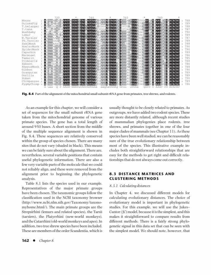
As an example for this chapter, we will consider aset of sequences for the small subunit rRNA genetaken from the mitochondrial genome of various primate species. The gene has a total length ofaround 950 bases. A short section from the middle of the multiple sequence alignment is shown in Fig. 8.4. These sequences are relatively conservedwithin the group of species chosen. There are manysites that do not vary (shaded in black). This meanswe can be fairly sure about the alignment. There are,nevertheless, several variable positions that containuseful phylogenetic information. There are also afew very variable parts of the molecule that we couldnot reliably align, and these were removed from thealignment prior to beginning the phylogenetic analysis.

Table 8.1 lists the species used in our example.Representatives of the major primate groups have been chosen. The taxonomic groups follow theclassification used in the NCBI taxonomy browser(http://www.ncbi.nlm.nih.gov/Taxonomy/taxono-myhome.html/). The main primate groups are theStrepsirhini (lemurs and related species), the Tarsii(tarsiers), the Platyrrhini (new-world monkeys),and the Catarrhini (old-world monkeys and apes). Inaddition, two tree shrew species have been included.These are members of the order Scandentia, which is

usually thought to be closely related to primates. Asoutgroups, we have added two rodent species. Theseare more distantly related, although recent studiesof mammalian phylogenies place rodents, treeshrews, and primates together in one of the fourmajor clades of mammals (see Chapter 11). As thesespecies have been well studied, we can be reasonablysure of the true evolutionary relationship betweenmost of the species. This illustrative example in-cludes both straightforward relationships that areeasy for the methods to get right and difficult rela-tionships that do not always come out correctly.

8.3 DISTANCE MATRICES ANDCLUSTERING METHODS

8.3.1 Calculating distances

In Chapter 4, we discussed different models for calculating evolutionary distances. The choice ofevolutionary model is important in phylogeneticstudies. For this example, we will use the Jukes–Cantor ( JC) model, because it is the simplest, and thismakes it straightforward to compare results fromdifferent methods. There is a fairly strong phylo-genetic signal in this data set that can be seen withthe simplest model. We should note, however, that

162 l Chapter 8

720 * 740 * 760 * 780 *Mouse : ACUAAAGGACUAAGGAGGAUUUAGUAGUAAAUUAAGAAUAGAGAGCUUAAUUGAAUUGAGCAAUGAAGUACGCACACAC : 788GuineaPig : AUUCAAGAUCUAAGGAGGAUUUAGUAGUAAAUUAAGAAUAGAGAGCUUGAUUGAACUAGGCCAUGAAGCACGUACACAC : 789T.belanger : ACUAUGAGUCCAAGGAGGAUUUAGCAGUAAGUCGGAAAUAGAGAGUCCGACUGAAUUAGGCCAUAAAGCACGCACACAC : 788T.tana : AACUAUGGUGUAAGGAGGAUUUAGCAGUAAACCGGAAAUAGAGAGUCCAGUUGAAUAAGGCCAUAAAGCACGCACACAC : 787Bushbaby : ACAAUUGGCAAAAGGCGGAUUUAGUAGUAAAUUAAGAAUAGAGAGCUUAAUUGAAUAGGGCAAUGAAGCACGCACACAC : 790Lemur : ACUAAAAGCCAAAGGAGGAUUUAGCAGUAAAUUAAGAAUAGAGAGCUUAAUUGAAUAGGGCCAUGAAGCACGCACACAC : 789W.Tarsier : AAUAAAAGUUAAAGGAGGAUUUAGCAGUAAACCAAGAAUAGAGAGCUUGAUUGAAAAAGGCCAUGAAGCACGCACACAC : 787Ph.Tarsier : AAUAAGAAUUAAAGGAGGAUUUAGUAGUAAAUCAAGAAUAGAGAGCUUGAUUGAAAUAGGCCAUGAAGCACGCACACAC : 789SakiMonk : ACUAAAAACCAAAGGUGGAUUUAGCAGUAAAUCGAGAAUAGAGAGCUCGAUUGAAACAGGCCAUUAAGCACGCACACAC : 788HowlerMonk : AUUAAAGGUCCAAGGUGGAUUUAGCAGUAAAUCAAGAAUAGAGAGCUUGAUUGAAACAGGCCAUUAAGCACGCACACAC : 790SpiderMonk : AUUAAAGGCCCAAGGUGGAUCUAGCAGUAAAUCAAGAAUAGAGAGCUUGAUUGAAGCAGGCCAUUAAGCACGCACACAC : 790Capuchin : AUUAAAGGCCCAAGGUGGAUUUAGCAGUAAAUCAAGAAUAGAGAGCUUGACUGAAGCAGGCCAUUAAGCACGCACACAC : 789Marmoset : AUUAAGGGCCCAAGGUGGAUUUAGCAGUAAACCAAGAAUAGAGAGCUUGAUUGAAACAGGCCAUUAAGCACGCACACAC : 786Tamarin : AUUAAGAGUCCAAGGUGGAUUUAGCAGUAAACCAAGAAUAGAGAGCUUGAUUGAAGCAGGCCAUUAAGCGCGCACACAC : 785Proboscis : ACUAAGAGCCCAAGGAGGAUUUAGUAGUAAAUUAAGAAUAGACUGCUUAAUUGACUUAGGCCAUGAAGCAUGCACACAC : 788Baboon : AUUAGGAGCCCAAGGAGGAUUUAGCAGUAAAUUAAGAAUAGAGUGCUUAAUUGAACUAGGCCAUAAAGCACGCACACAC : 786RhesusMonk : AUUAAGGGUCCAAGGAGGAUUUAGCAGUAAAUUAAGAAUAGAGUGCUUAAUUGAACCAGGCCAUAAAGCGCGCACACAC : 788Gibbon : ACUGAGGGUCGAAGGAGGAUUUAGCAGUAAAUUAAGAAUAGAGUGCUUAGUUGAACAAGGCCCUGAAGCGCGUACACAC : 790Orangutan : AUUGAAGGUCGAAGGUGGAUUUAGCAGUAAACUAAGAGUAGAGUGCUUAGUUGAACAAGGCCCUGAAGCGCGUACACAC : 789Gorilla : ACUAAGGGUAGAAGGUGGAUUUAGCAGUAAACUAAGAGUAGAGUGCUUAGUUGAACAGGGCCCUGAAGCGCGUACACAC : 789Human : ACUAAGGGUCGAAGGUGGAUUUAGCAGUAAACUAAGAGUAGAGUGCUUAGUUGAACAGGGCCCUGAAGCGCGUACACAC : 790Chimpanzee : ACUAAGGGUCGAAGGUGGAUUUAGCAGUAAACUAAGAGUAGAGUGCUUAGUUGAACAGGGCCCUGAAGCGCGUACACAC : 789PygmyChimp : ACUAAGGGUCGAAGGUGGAUUUAGCAGUAAACUAAGAGUAGAGUGCUUAGUUGAACAGGGCCCUGAAGCGCGUACACAC : 786

A uaa g c AAGG GGAUuUAGcAGUAAa aagAaUAGAg Gcuu uUGAa gGCc U AAGc cG ACACAC

Fig. 8.4 Part of the alignment of the mitochondrial small subunit rRNA gene from primates, tree shrews, and rodents.

BAMC08 09/03/2009 16:39 Page 162

the JC model is not often used in modern studies. Theimplicit assumption of the JC model that the fourbases have equal frequencies is definitely not true inthe rRNA genes studied here, so some of the morecomplex models discussed in Chapter 4 wouldalmost certainly give better fits to the data than theJC model.

From a multiple alignment, we can easily calculatethe JC distance between each pair of sequences usingEq. (4.4). We can then construct a matrix whose elements, dij, are the distances between each pair ofspecies, i and j. The matrix for the sequences fromthe Catarrhini is shown in Fig. 8.5. The matrix issymmetric (i.e., dij must be equal to dji) and the diago-nal elements, dii, are zero, because the distance of asequence from itself must be zero. To get an idea of

scale, the human to chimpanzee distance is 2.77%.The smallest distance is 1.49% between chimpanzeeand pygmy chimpanzee, and the largest distance inthe figure is the orangutan to proboscis monkey dis-tance, which is close to 20%. The distances from themouse to the primates (not shown) are around26–30%. In fact, mitochondrial sequences are relat-ively rapidly evolving. If we had used a nuclear gene,we would have obtained smaller distances for thesame set of species. It should also be rememberedthat we have removed some of the most rapidlychanging regions of the molecule from the align-ment prior to calculating these distances becausethese regions were deemed to be unreliably aligned.If these parts had not been removed, all the distanceswould have come out slightly higher.

Phylogenetic methods l 163

Taxon name Species

Rodentia Mus musculus (Mouse)Cavia porcellus (Guinea pig)

Scandentia Tupaia belangeri (Northern tree shrew)Tupaia tana (Large tree shrew)

PrimatesStrepsirhini (Prosimians) Lemur catta (Ringtailed lemur)

Otolemur crassicaudatus (Thick-tailed bushbaby)Tarsii (Tarsiers) Tarsius syrichta (Philippine tarsier)

Tarsius bancanus (Western tarsier)Platyrrhini (New-world monkeys)

Cebidae Pithecia pithecia (White-faced Saki monkey)Cebus apella (Brown capuchin)Alouatta seniculus (Howler monkey)Ateles sp. (Spider monkey)

CallitrichidaeCallithrix pygmaea (Pygmy marmoset)Leontopithecus rosalia (Golden lion tamarin)

CatarrhiniCercopithecidae (Old-world monkeys) Nasalis larvatus (Proboscis monkey)

Macaca mulatta (Rhesus monkey)Papio hamadryas (Baboon)

Hylobatidae Hylobates lar (Gibbon)Hominidae Pongo pygmaeus (Orangutan)

Gorilla gorilla (Gorilla)Pan troglodytes (Chimpanzee)Pan paniscus (Pygmy chimpanzee)Homo sapiens (Human)

Table 8.1 Classification of species used in the examples in this chapter.

BAMC08 09/03/2009 16:39 Page 163

A distance matrix can be used as the input to aclustering method. Algorithms for clustering workin the following way:1 Join the closest two clusters to form a single largercluster.2 Recalculate distances between all the clusters.3 Repeat steps 1 and 2 until all species have beenconnected to a single cluster.Initially, each species forms a cluster on its own. Theclusters get bigger during the process, until they areall connected to a single tree. We already discussedclustering methods in a different context in Chap-ter 2. We will discuss two clustering methods herethat are particularly relevant for phylogenetics: theUPGMA (unweighted pair group method with arith-metic mean) and neighbor-joining methods.

8.3.2 The UPGMA method

This is one of a family of hierarchical clusteringmethods described by Sneath and Sokal (1977). It has some important limitations, which means thatit is now not often used in phylogenetic researchstudies. However, we will discuss it first, because it isconceptually the simplest phylogenetic method.

Step 1 of the clustering algorithm is to connect thetwo closest species, in this case the chimpanzee andthe pygmy chimpanzee. Step 2 is to calculate the distance from the chimpanzee/pygmy chimpanzeecluster to all the other species. In the UPGMAmethod, the distance between two clusters is simplydefined as the mean of the distances between speciesin the two clusters. For example, the distance of

human from the chimpanzee/pygmy chimpanzeecluster is the mean of the human–chimpanzee andhuman–pygmy chimpanzee distances. If, at somepoint, we want to calculate the distance between acluster with two species and a cluster with threespecies, then this will be the average of six (= 2 × 3)numbers. Defining the distances between clusters asan arithmetic mean in this way is a fairly obviousdefinition. However, there are many other ways ofdoing it. It is this definition that distinguishes theUPGMA from the other clustering methods given bySneath and Sokal (1977).

Proceeding with our primates, it turns out thatthe distance from the human to the two chim-panzees is smaller than any of the other remainingdistances, and therefore the next step is to connectthese together. After repeating the steps of the clustering algorithm, we eventually obtain the treein Fig. 8.6. This is a rooted tree, with branch lengthsthat are proportional to the inferred amount of time separating the species, i.e., the UPGMA methodassumes that there is a strict molecular clock andthat all species evolve at the same rate. The lengthsof the branches are determined by the heights of theinternal nodes in the tree above the base line. Theheight of the node connecting chimpanzee andpygmy chimpanzee is 0.0074. This is half the dis-tance between the two species. The factor of a halfarises because we are assuming that half of thechanges separating the two species occurred on thebranch leading to one species and half occurred onthe other. Now consider the earliest node in Fig. 8.6,which connects the old-world monkeys to the apes.

164 l Chapter 8

Fig. 8.5 The JC distance matrix for the some of the rRNA sequences in Fig. 8.4. The matrix has been divided into sections in orderto indicate the most important split within the Catarrhini group: that between the old-world monkeys and the apes.

BAMC08 09/03/2009 16:39 Page 164

The distance between these groups is the mean ofthe 18 numbers in the top right section of the matrixin Fig. 8.5. The height of the node is half this meandistance, which is 0.0865. Notice that this methodtells us that the root of the tree is at the point wherethe last two clusters are connected – in this case theold-world monkeys and the apes. Most other meth-ods do not give the position of the root.

If we pick any three species from the UPGMA tree,there are always two that are more closely related toeach other than to the third. According to the tree,the distances from the third species to the first andsecond species are equal to one another, becausethese two distances are both determined by the samebranch point. The distance from the first to the second species is smaller than this. This property iscalled ultrametricity: whichever three species wetake from the UPGMA tree, the two largest of thethree distances between these species will be equal.It is clear that if we consider divergence timesbetween species, as in Fig. 8.1(a), the two largestdivergence times for any three species must be equal.Thus, divergence times form an exactly ultrametricmatrix. If sequences evolve according to a molecularclock, the distances between them will be approx-imately ultrametric, but not exactly so. This isbecause substitutions in gene sequences are random

events. The two lineages descending from a node willhave the same number of substitutions on average,but in any one particular case, one lineage will bychance have slightly more substitutions than theother. Thus, even in an ideal world where the mole-cular clock is exactly true, the distances betweensequences will only be approximately ultrametric.In our case, if the matrix were exactly ultrametric,all the 18 distances in the top right section of thematrix would be exactly equal, whereas in realitythey are only approximately equal. What the UPGMAmethod does is to find an ultrametric tree such thatthe distances measured on the tree are a close appro-ximation to the distances in the original matrix.

In the real world, it may not be just chance thatmakes distances violate the ultrametric rule. Ifspecies evolve at different rates, then we get trees likeFig. 8.2, rather than Fig. 8.1. In this case, there is noreason why the two largest distances of any group ofthree must be equal. The problem with the UPGMAmethod is that it forces the species to lie on an ultra-metric tree, even when the original distance matrixis far from ultrametric. In this case, the resulting tree is usually wrong. In many real data sets, themolecular clock assumption may not be a good oneand, for this reason, UPGMA is often not a reliablemethod. We have discussed UPGMA because it is

Phylogenetic methods l 165

0.0074

0.0865

Baboon

Proboscis monkey

Gibbon

Rhesus monkey

Gorilla

Orangutan

Chimpanzee

Pygmy chimp

Human

Fig. 8.6 Tree obtained using theUPGMA method with the matrix in Fig.8.5. The PHYLIP package was used fortree construction (Felsenstein 2001)and the Treeview program (Page 2001)was used to prepare the figure.

BAMC08 09/03/2009 16:39 Page 165

conceptually one of the simplest clustering methods.Although it would not be recommended for mostserious phylogenetic studies, it is nevertheless import-ant to understand how it works and how it differsfrom other methods. For the species in Fig. 8.6, theUPGMA result corresponds to what is generallybelieved to be true. This is not bad, considering weused the simplest possible method of calculating dis-tances and the simplest possible clustering method.This indicates that there is quite a strong phylo-genetic signal in the sequences from the Catarrhini.When the more distantly related species from Table 8.1 were included, the UPGMA did not givethe correct topology, and therefore we have notshown these species in Fig. 8.6.

8.3.3 The neighbor-joining method

Neighbor joining (NJ) (Saitou and Nei 1987) is aclustering method that produces unrooted trees,rather than the rooted ones produced by UPGMA.There is a property of unrooted trees called additiv-ity that we need to introduce at this point. A tree is said to be additive if the distances between thespecies on the tips of the tree are equal to the sum of the lengths of the branches that connect them. Forexample, in Fig. 8.3(a), dAC = dAi + dij + djC. A distancematrix is said to be additive if it is possible to find atree with specified branch lengths such that all thepairwise distances in the matrix are exactly equal todistances measured by summing along the branchesof the tree. Additivity is a less restrictive conditionthan ultrametricity. If a distance matrix is ultramet-ric, it is also additive, but the reverse is not necessar-ily true. The NJ method constructs an additive treesuch that the distances between species measuredon the tree are a good approximation to the dis-tances in the original matrix. If the original matrix

is exactly additive, NJ is guaranteed to give the correct tree, just as UPGMA is guaranteed to give the correct tree if the original distance matrix isultrametric. However, in the real world, the dis-tances will not be exactly additive; therefore, NJ isjust one approximation.

Two species are said to be neighbors on anunrooted tree if they are connected via a single inter-nal node. In Fig. 8.3(a), A and B are neighbors, C andD are neighbors, but A and C are not neighbors. TheNJ method begins with a set of disconnected tipnodes representing the known sequences. These are shown as white circles in Fig. 8.7(a). We knowthe distances between all these nodes, as specified inthe input distance matrix. The method chooses twonodes, i and j, that are neighbors and connects themby introducing a new internal white node, n. Theoriginal nodes, i and j, are now eliminated from the problem because they are already connected tothe growing tree. They have been colored black inFig. 8.7(b). We now have a set of disconnected whitenodes that has one fewer than before. This processcan be repeated until all the nodes are connected to a single tree. Details are given in Box 8.1.

Applying the NJ method to the distance matrix forthe primate sequences gives the result in Fig. 8.8(a).This tree topology agrees with what we expectedfrom the taxonomic classification (Table 8.1) inmost respects. The Catarrhini and the Platyrrhiniform two well-defined groups. The lemur and bush-baby cluster together, as do the two tarsiers, the twotree shrews and the two rodents. The result is easierto interpret if we place the root of the tree on thebranch leading to the rodents and redraw the tree asin Fig. 8.8(b). It should be remembered, however,that the NJ method does not tell us where to place theroot – we must use prior knowledge to decide whereto put it.

166 l Chapter 8

(a) (b)

j

i

n n

k

Fig. 8.7 Step one of the neighbor-joining method.

BAMC08 09/03/2009 16:39 Page 166

The part of the tree covering the Catarrhini is sim-ilar to the result of the UPGMA (Fig. 8.6). Thebranching order within the Platyrrhini is worth not-ing. The marmoset and the tamarin cluster together.These are members of the Callitrichidae family in theNCBI taxonomy. In contrast, the other four new-world monkeys, classified as Cebidae, do not form amonophyletic group, and this suggests that it is notevolutionarily meaningful to group these species inthe Cebidae taxon. We should beware of jumping toconclusions, because so far we have only considereda single simple phylogenetic method. However, in allthe methods we tried, the same branching patternfor the new-world monkeys was found. Therefore, we

can be reasonably confident that the Cebidae are not monophyletic, according to the evidence fromthe rRNA gene. A more detailed study of phylo-genetics of the Platyrrhini has been carried out byHorovitz, Zardoya, and Meyer (1998). Their results,using small subunit rRNA sequences, agree withour Fig. 8.8(a) in that the Saki monkeys form theearliest-branching new-world monkeys. However,results using different gene sequences and morpho-logical evidence give different branching patterns.Thus, the Platyrrhini phylogeny is still not fullyresolved.

There is another, more serious, problem with Fig. 8.8(b): the tree shrews are apparently the sister

Phylogenetic methods l 167

BOX 8.1Calculation of distances in theneighbor-joining method

When we introduce the new node, n, we need to knowits distance from all the other nodes. To calculate thesedistances, we will assume the distances are additive.Consider one particular node, k, among the nodes still tobe connected. We may write (from Fig. 8.7a):

dij = din + djn; dik = din + dkn; djk = djn + dkn (8.1)

We may solve these simultaneous equations to find thedistance of k from the new node:

dkn = (dik + djk − dij) (8.2)

This equation can be used for each of the unconnectednodes, k. We now need the distances din and djn. Fromthe simultaneous Eqs. (8.1), we can write:

dIn = (dij + dik − djK) (8.3)

The problem with this is that it depends on one particularnode, k. We could call any of the disconnected nodes kand we would get a slightly different answer for din foreach one. To avoid this problem, we define the quantities

(8.4) r

Nd r

Ndi ik

kj jk

k

;

=−

=−∑ ∑1

21

2

12

12

Here, N is the total number of white nodes. The best estimate of din is to average Eq. (8.3) over all the N – 2disconnected nodes k. This gives:

din = (dij + ri − rj) (8.5)

Obviously, because of additivity, djn = dij − din. We havenow reached the situation in Fig. 8.7(b), where we havea reduced set of N − 1 white nodes and therefore we canrepeat the whole procedure again.

However, we did not yet say how to choose the twoneighboring nodes, i and j, to connect in the first place.It might seem natural to choose the two with the smallestdistance, dij, as we would with UPGMA. Unfortunately,there is a problem that is illustrated in Fig. 8.3(a). Theclosest two species in this tree are B and D, because thereare short branches connecting them, but B and D arenot neighbors, so it would be wrong to connect them.The NJ method has a way of getting around this. We calculate modified distances,

d *ij = dij − ri − rj (8.6)

and we choose the two species with the smallest d *ijrather than the smallest dij. It has been shown (Saitouand Nei 1987, see also Durbin et al. 1998) that if the dis-tance matrix is additive, then the two species chosen bythis rule must be neighbors.

12

BAMC08 09/03/2009 16:39 Page 167

0.1

0.1

90

24

75

45

100

100

10052

9865

53

100

100

100

100

92

98

100

71Human

Chimpanzee

Pygmy chimp

Gorilla

Rhesus monkey

Gibbon

Proboscis monkey

Baboon

Howler monkey

Spider monkey

Tamarin

Marmoset

Saki monkey

Capuchin

Western tarsier

Westerntarsier

Philippine tarsier

Philippine tarsier

Bushbaby

Bushbaby

Lemur

Lemur

Northern Tree shrew

Northern Tree shrew

Large Tree shrew

Large Tree shrew

Mouse

Mouse

Guinea pig

Guinea pig

Orangutan

96

(b)

(a)

HumanChimpanzee

Pygmy chimp

Gorilla

Rhesus monkey

GibbonProboscis monkey

Baboon

Howler monkeySpider monkey

TamarinMarmoset

Saki monkey

Capuchin

Orangutan

Fig. 8.8 Tree obtained with theneighbor-joining method and JCdistances. (a) Unrooted. (b) Rooted with the rodents as outgroup, and withbootstrap percentages added.

BAMC08 09/03/2009 16:39 Page 168

group to the tarsiers. This is almost certainly wrong.It would mean that the primates were not a mono-phyletic group and that the order Scandentia shouldactually be included within the primates. We wouldnot be willing to propose this phylogenetic arrange-ment, given the morphological evidence that favorsplacing tree shrews as a separate group outside theprimates. The NJ tree must be misleading us in thiscase, and we will return to this point below.

To summarize: the NJ method is a practical, rapidway of getting a fairly reliable result and, as such, it is often used in real phylogenetic studies. The clustering algorithm runs in a time that is O(N 2). In practice, the result can be obtained almost in-stantaneously, even when there are very large numbers of sequences, whereas the more complexmethods described below can take large amounts of computer time. As stated above, NJ is exact if thedistance matrix is additive, and it stands a goodchance of giving the correct tree topology if thematrix is not far from additive. If the input distancesare not close to being additive (e.g., because an inap-propriate method of calculation of the pairwise dis-tances was used, or because the sequences were notproperly aligned), then NJ will give the wrong tree.

8.4 BOOTSTRAPPING

You will have noticed the numbers that appeared onthe internal nodes of the tree in Fig. 8.8(b). These arecalled bootstrap percentages. Bootstrapping is amethod of assessing the reliability of trees, intro-duced by Felsenstein (1985), and has since becomea standard tool in phylogenetics.

Substitutions in sequences are random events.Even if the sequences are evolving in a way that iswell described by the model of evolution that we use,the number of substitutions occurring on anybranch of a real tree can deviate substantially fromthe mean value expected according to the model.This means that the distances we measure betweensequences are subject to chance fluctuations. Wewould like to know whether these fluctuations areinfluencing the tree that we obtain. The bootstrap-ping method answers this question by deliberatelyconstructing sequence data sets that differ by somesmall random fluctuations from the real sequences.The method is then repeated on the randomizedsequences in order to see whether the same treetopology is obtained.

The randomized sequences are constructed bysampling columns from the original sequence align-ment, as shown in Fig. 8.9. The randomizedsequences are the same length as the real ones. Eachcolumn in the randomized sequences is constructedby copying one random column from the originalsequence alignment. During this sampling process,some columns happen to be chosen more than once,while some columns happen not to be chosen at all (technically, this is known as “sampling withreplacement”). This means that the random sequ-ences contain slightly different information from the real ones. When we construct a tree with therandomized sequences, we are not guaranteed to getthe same answer as before. If the phylogenetic signalin the data is strong, there is a lot of informationabout the degree of relatedness of the species spreadalong the whole length of the sequence. There-fore, resampling should make very little difference.

Phylogenetic methods l 169

Fig. 8.9 An illustration of resamplingcolumns for the bootstrapping method.

BAMC08 09/03/2009 16:39 Page 169

However, sometimes the signal indicating one treetopology over another may be rather weak. In thiscase, the noise that we introduce to the data whenwe resample may be sufficient to cause the tree-construction method to give a different result. Notethat the resampling procedure is not equivalent tojust reshuffling the columns of the original align-ment. Phylogenetic methods treat each columnindependently, so a reshuffled alignment would giveexactly the same answer as the original sequences,and would not tell us anything.

To carry out bootstrapping analysis, many sets ofrandomized sequences are constructed (usually 100or 1,000). The tree-construction method is repeatedon each set of sequences to produce a set of possibletrees, some of which will be equivalent to the ori-ginal tree and some of which will be different. Wethen look at each group of species in the original treeand we determine what percentage of the random-ized trees contain this same group. This percentagegives us a measure of confidence that those speciesreally do form a related group. The bootstrap resultsfor the primate sequences using the NJ method areshown in Fig. 8.8(b). 1,000 replicates were done,but the numbers are shown as percentages in thefigure. There are many strongly supported clades inthis tree. For example, the taxa Hominidae, Cercopit-hecidae, Catarrhini, and Platyrrhini (as defined inTable 8.1) all have 100% bootstrap support, as dothe tarsiers and the tree shrews. The prosimiangroup (lemur and bushbaby) also has 90% support.Other relationships in the tree are much less certain.Although the new-world monkeys, as a group, have100% support, there are several low bootstrap val-ues within the group, indicating that the branchingorder within the new-world monkeys is not wellresolved by this method. The weakest point in thisphylogeny is the very low value of 24% at the nodelinking the prosimians, tarsiers, and tree shrews. Wereally cannot be sure at all that these three groupsform a clade. Indeed, other evidence tells us thatmost likely they do not, as discussed above. There isno precise rule to say how high a bootstrap percent-age has to be before we can be sure that the group ofspecies in question forms a “true” clade, althoughvalues greater than 70% are often thought to be

reasonably strong evidence. It is slightly worryingthat the grouping of tarsiers and tree shrews has abootstrap value of 75%, because this is very likely anincorrect relationship. We will see below that thisapparent relationship goes away when we use amore realistic model of sequence evolution. For themoment, we note that bootstrap numbers need to betreated with caution. They are often a very usefulindication of the reliability of different parts of a phylogenetic tree, but they do not “prove” anythingconclusively.

Let us consider one particular point in Fig. 8.8(b)in more detail – the 71% value for the human +chimpanzee + pygmy chimpanzee clade. This valueis sandwiched between two very high figures, i.e.,the two chimpanzees almost always form a clade(96%), and the group gorilla + human + chimpanzee+ pygmy chimpanzee always forms a clade. Thus,what is at stake is the relationship between gorilla,human, and the chimpanzees. The topology shownhas the gorilla as the most distantly related of thesethree – this can be denoted as (gorilla,(human,chimpanzees)). The other two topologies – (human,(gorilla, chimpanzees)) and (chimpanzees,(gorilla,human)) – also turn up occasionally in the bootstrapreplicates, but much less frequently than the topo-logy in the figure. In fact, it is now generally agreedthat the humans and chimpanzees are the closest of the three, although there has been considerablediscussion in the past (see Hasegawa, Kishino, andYano (1985) and references therein).

Bootstrap results are often presented in the form ofconsensus trees. The frequency of occurrence ofeach possible clade in the set of bootstrap trees isdetermined, and clades are ranked in descendingorder of frequency. The consensus tree is con-structed by adding clades one at a time working fromthe top of the ranking list. Each clade added is theone with the highest frequency that is consistentwith all the clades already added. The final con-sensus topology may differ slightly from the treeobtained with the original full set of data. It is then amatter of choice whether to present the original treelabeled with bootstrap percentages for the cladescontained in that tree, or to present the consensustree, which will tend to contain clades with slightly

170 l Chapter 8

BAMC08 09/03/2009 16:39 Page 170

higher bootstrap values that were not present in theoriginal tree. Well-determined clades, with highbootstrap values, will almost always occur in boththe consensus and the original tree, so this issueaffects only the way the results are presented for theleast well-determined parts of the tree.

8.5 TREE OPTIMIZATION CRITERIAAND TREE SEARCH METHODS

8.5.1 Criteria for judging trees

As explained above, NJ constructs an additive treesuch that the distances measured on the tree areapproximately equal to the distances specified in thedistance matrix. It is possible to define the followingfunction, E, which measures the error made in thisprocess:

(8.7)

where dij is the distance specified in the distancematrix, dij

tree is the distance measured along thebranches of the tree, and the sum runs over all pairsof species. This function is the sum of the squares ofthe relative errors made in each of the pairwise dis-tances. E can be used as a criterion for evaluatingtrees. Fitch and Margoliash (1967) proposed a phylo-genetic method that consists of searching for the treethat minimizes the function E. This can be consid-ered as finding the additive tree that differs least fromthe input data. If the distance matrix is exactly addi-tive, then it is possible to find a tree such that everyterm in the sum is exactly zero. However, usually,this is not possible, because the number of pairs ofspecies is N(N − 1)/2, while the number of indepen-dent branch lengths to be optimized on an unrootedtree is only 2N − 3. Therefore, the method finds a treefor which E is as small as possible, but it cannot set Eto zero exactly.

Clustering methods like NJ and UPGMA have awell-defined algorithm for constructing a tree. How-ever, they do not have a well-defined criterion bywhich trees may be compared. Such a criterion is notnecessary because clustering algorithms give rise

Ed d

dij ij

tree

iji j

( )

,

=−

∑2

2

automatically to a single tree as output. In contrast,the Fitch–Margoliash method has a well-defined cri-terion for judging trees (the best tree is the one forwhich E is the smallest), but there is no well-definedalgorithm for constructing the best tree. It is neces-sary to use a program that constructs many alter-native trees and then tests each one out using thecriterion. This means that the Fitch–Margoliashmethod is much slower than NJ. In practice, if thematrix is approximately additive, NJ will give a verysimilar answer to Fitch–Margoliash in a shorter time.On the other hand, if the matrix is far from beingadditive, then neither of these methods is appropriate,and both are likely to give inaccurate tree topologies.

The idea of testing alternative trees using somecriterion of optimality is a key one, because two veryimportant phylogenetic methods, the maximum-likelihood and the parsimony methods, both use thisprinciple. In brief, the maximum-likelihood criterionis to choose the tree on which the likelihood ofobserving the given sequences is highest, while theparsimony criterion is to choose the tree for whichthe fewest number of substitutions are required inthe sequences. These criteria will be discussed fullyin the following sections. In this section, we wish toconsider how we might search for candidate trees.The method for tree searching is independent of thecriterion used for judging the trees.

8.5.2 Moves in tree space

There is an enormous number of tree topologies,even for very small numbers of species, as shown inTable 8.2. The notation !! means the product of the odd numbers, so that U7 = 9!! = 9 × 7 × 5 × 3 × 1 = 945. Only if the number of species is very small(i.e., less than about eight) will it be possible toexhaustively test every tree. More usually we willneed heuristic search programs. It is useful to thinkof “tree space”, which is the set of all possible treetopologies. Two trees are usually considered to beneighboring points in tree space if they differ by a topology change known as a nearest-neighborinterchange (NNI). To make an NNI, an internalbranch of a tree is selected (a branch has been high-lighted in bold in Tree 1 of Fig. 8.10). There are two

Phylogenetic methods l 171

BAMC08 09/03/2009 16:39 Page 171

subtrees linked to each end of this branch. A subtreemay be either a single species (like A), or a branchingstructure that may contain any number of species(like D + E). The NNI move consists of swapping anyone subtree from one end of the internal branch withany one subtree from the other end. In Fig. 8.10,Tree 2 is obtained by swapping B and C, and Tree 3 isobtained by swapping A and C. We could also swapthe D + E group with either A or B, but this wouldalso create either Tree 2 or 3. Thus, Trees 1, 2, and 3are all neighbors of each other by a single NNI about

the highlighted branch, and there are no other treesthat can be formed by making rearrangementsabout this same branch. Tree 4 is not a neighbor ofTree 1, as it is not accessible by a single NNI. Theshortest path from 1 to 4 involves two NNIs (can youwork out what these are?). It is possible to create anyrearrangement of a tree by a succession of NNIs.

Moving from Tree 1 to Tree 4 is an example ofanother type of topology change called subtree prun-ing and regrafting (SPR). This consists of choosingany subtree in the original tree (in this example, just the single species D), cutting it from the tree, and then reconnecting it to any of the branches remaining on the original tree (in this example, the branch leading to B). The SPR is one type of a long-range move in tree space. Another possiblelong-range move, described by Swofford et al.(1996), is tree bisection and reconnection, in whichan internal branch is selected and removed, thusforming two separate subtrees. These subtrees arereconnected by selecting one branch at randomfrom each subtree and connecting these by a newinternal branch.

We now return to the question of searching treespace to find the tree that is optimal by some criter-ion, such as likelihood, parsimony, or least-squareserror E. Suppose we have an initial guess at an

172 l Chapter 8

No. of species No. of distinct tree topologies(N) Unrooted (UN) Rooted (RN)

3 1 34 3 155 15 1056 105 9457 945 10,3958 10,395 135,1359 135,135 2.0 × 106

10 2.0 × 106 3.4 × 107

N (2N − 5)!! (2N − 3)!!

Table 8.2 How many trees topologies are there?

B

A

C

D

E

1

B

A

C

D

E

4

C

A

B

D

E

2

B

C

A

D

E

3 Fig. 8.10 Examples of changes in treetopology. Trees 1, 2, and 3 all differfrom each other by a single nearestneighbor interchange. Tree 4 differsfrom tree 1 by a subtree pruning andregrafting operation.

BAMC08 09/03/2009 16:39 Page 172

optimum tree. This could be the tree produced by adistance-matrix method, for example. We wouldexpect this tree to be “not too bad”, according to ouroptimization criterion; therefore, we would expectthat looking at other trees that are similar to this onemight be a sensible strategy for finding the optimumtree. One way of proceeding is to test trees that areneighbors of our current tree. If we find a neighbor-ing tree that is better, then we move to this new treeand search the neighbors of the new tree. We keepdoing this until we reach a tree that is a local opti-mum, i.e., it has no neighbors that are better than it.This is a hill-climbing algorithm, because we alwaysmove “uphill” to a better tree at each step. We can-not guarantee that the local optimum we reach willbe the global optimum tree that we are looking for.One way to check this would be to try hill climbingfrom lots of different starting points. A possible wayto generate the starting points is by sequential addi-tion of species. Suppose the species are listed in a ran-dom order. There is only one unrooted tree topologyfor the first three species in the list. We then add onespecies at a time to the tree. Each species is added byconnecting it in the optimal way to the tree that isalready present, until all species have been added.We can then try to improve the tree by hill climbing,using NNIs, until a local optimum is reached. Thisprocedure can be repeated many times, starting withdifferent random orders of species. We may obtainmany different local optima. If we continue for longenough, then it is very likely that the best of the localoptima that we find will be the global optimum. Thisis a heuristic search procedure, so we cannot guar-antee that we have found the global optimum. Allwe can do is hope that if we have run the search for along time without finding any improvement, thenwe have probably found the best tree.

The definition of a local optimum tree depends onthe definition of what is a neighbor. If we use NNIs todefine neighbors, then we may reach trees that can-not be improved by NNIs, but that could be improvedby longer-range moves. In principle, long-rangemoves could also be included in the search strategy(and some programs do this). However, the problemwith long-range moves tends to be that they arerather disruptive. If we already have a fairly good

tree, then most long-range moves will create a treethat is much worse, and they will thus be a waste ofcomputer time. The longest-range move we couldimagine would be to try a completely random treeeach time. We would eventually hit on the globaloptimum by this strategy, but it would be a very slowand inefficient search procedure. Most real searchprograms use a combination of NNIs and slightlylonger-range moves that has been tested and foundto be reasonably efficient at finding optimal trees asquickly as possible. We also note, at this point, thatsearch strategies are not limited to moving uphill. Ifwe occasionally allow downhill moves, then thismay prevent us getting stuck on very poor localoptima, and allow better optima to be found morequickly. The Markov Chain Monte Carlo method,discussed in Section 8.8, is a way of searching treespace that allows both uphill and downhill moves.

8.6 THE MAXIMUM-LIKELIHOODCRITERION

Given a model of sequence evolution and a proposedtree structure, we can calculate the likelihood thatthe known sequences would have evolved on thattree. The maximum-likelihood (ML) criterion is tochoose the tree that maximizes this likelihood(Felsenstein 1981). An algorithm for doing this isdiscussed in Box 8.2. Three qualitatively differenttypes of parameter must be specified to calculate thelikelihood of a sequence set on a tree: the tree topo-logy; the branch lengths; and the values of theparameters in the rate matrix (base frequencies,transition/transversion ratio, etc.). It is possible tooptimize all of these things at the same time. Pro-grams are available that will search tree space making changes that alter all three types of para-meter, and attempt to find the ML solution. On theother hand, it is possible to fix some things while theothers are optimized. For example, we might want tofind the ML tree topology and branch lengths, whilekeeping the rate-matrix parameters fixed at particu-lar numerical values.

The ML criterion can be used to distinguishbetween a set of tree topologies specified in advance.

Phylogenetic methods l 173

BAMC08 09/03/2009 16:39 Page 173

For example, the bootstrapping analysis using a distance-matrix method shows where the uncer-tainties lie in a tree; therefore, we might wish to testa set of alternative trees that differ in their branchingorders at the uncertain points in the tree. It is pos-

sible to estimate the value of the ML for each of theuser-specified trees, by allowing the branch lengthsand rate parameters to vary but keeping the topo-logy fixed. This gives a ranking of the specified trees.Often the likelihoods of several different trees will

174 l Chapter 8

BOX 8.2Calculating the likelihood of thedata on a given tree

Consider the calculation of the likelihood for a given site n.In Fig. 8.11, there are two tip nodes with known sequ-ences that happen to be A and G at this site. The likelihoodthat the common ancestor of these two had a base X is

Ln(X) = PXA(t1)PXG(t2) (8.8)

Here, the functions Pij(t) are the transition probabilitiescalculated using an appropriate model of sequence evo-lution, as described in Chapter 4. Four likelihoods arecalculated using Eq. (8.8) for the four possible values of X.We may now proceed to the node labeled Y, and calculate

(8.9)

For each of the four possible values of Y, we have tosum over the four possible values of X, weighting themby the likelihood of that value of X. For a node like W,

L Y P t L X P tn YG n YX

X

( ) ( ) ( ) ( )= ∑4 3

where both the descendant nodes are internal nodes, itis necessary to sum over the four possible values of boththese descendant nodes:

(8.10)

This procedure can be repeated until we get to theroot of the tree, so that we have the likelihoods for thebase occurring at the root node (in this tree, W is alreadythe root). We can now calculate the total likelihood, Ln,for site n by summing over the possible bases at the root.We assume that the prior probability of each base thatcould have existed at the root is given by the equilibriumfrequency of the bases, pW, according to the evolution-ary model. Hence,

(8.11)

This algorithm for calculating the likelihood of a givensite builds recursively from the tips towards the root. Infact, the final likelihood does not depend on the rootposition. When calculating the likelihood, the root canbe placed at any arbitrary position on the tree, becausethe likelihood always turns out the same.

The likelihood is calculated for each site in this way,and it is assumed that sites evolve independently.Therefore, the likelihood for the complete sequence set,Ltot, is the product of the likelihoods of the sites. It there-fore follows that the log of the likelihood is the sum ofthe logs of the site likelihoods

(8.12)

It is log-likelihood values that are usually quoted in theresults of ML programs. As there are very many possiblesequence sets that could evolve on any given tree, thelikelihood of the real data is always very much less than1. Therefore, ln Ltot is always a large negative number.The ML tree is the one with the least negative value.

ln ln L Ltot n

n

= ∑

L L Wn W n

W

( )= ∑ p

L W L Y P t L Z P tn n WY

ZYn WZ( ) ( ) ( ) ( ) ( )= ∑∑ 5 6

TGA G T

t1

t3

t5

t6

t4

t2

X

Y

W

Z

Fig. 8.11 An illustration of calculating the likelihood for asingle site on a given tree. Letters A, G, and T label bases onthe known sequences. Letters X, Y, Z, and W label unknownbases on internal nodes. The times (or equivalently, branchlengths) on each branch are labeled t1, t2, etc.

BAMC08 09/03/2009 16:39 Page 174

differ by only a small amount. It is then important todecide whether one tree is really better than thealternatives. This can be done using a test proposedby Kishino and Hasegawa (1989). The total log like-lihood is the sum of values from each site, as in Eq.(8.10). If the sites evolve independently, then we canestimate the error in the total log likelihood by calcu-lating the standard deviation of the log likelihoods ofthe sites. We can then compare two different trees,and ask whether the difference in log likelihoodsbetween the trees is significant in comparison to theerror in estimation of this difference.

We would now like to see what the ML criterionsays about the primate phylogeny example. Wehave used a search algorithm from our own phylo-geny package, PHASE ( Jow et al. 2002), to do this.There are several closely related groups of which weare already fairly certain. We are really interested inthe early branch points on the tree that define theway these closely related groups are related to oneanother. For the ML analysis, we specified the fol-lowing clades in advance:

1. (Mouse,Guinea Pig)

2. (Bushbaby,Lemur)

3. (Northern Tree Shrew,Large Tree

Shrew)

4. (Western Tarsier,Philippine

Tarsier)

5. (Saki Monkey,(Capuchin,((Tamarin,

Marmoset),(Howler Monkey,Spider

Monkey))))

6. ((Proboscis Monkey,(Baboon,Rhesus

Monkey)),(Gibbon,(Orangutan,(Gorilla,

(Human,(Chimpanzee,Pygmy

Chimpanzee))))))

Each of these clades is a rooted subtree that occurs on the NJ tree for which we are willing toassume that we know the correct branching order.There are 105 unrooted tree topologies that can be obtained by connecting these clades together. An ML algorithm was used to optimize the branchlengths and rate parameters for each of these 105topologies separately, and to find the ML topology.Note that this involves changing the branch lengths

within the clades, as well as the branch lengths on the internal branches connecting the clades;however, rearrangement of the species within theclades is not allowed. As this algorithm is an exhaust-ive search of topologies, we can be sure we havefound the correct ML solution (provided the cladeswere defined correctly at the outset). This algorithmalso has the advantage of being rapid, because thenumber of topologies is relatively small when thenumber of clades is small, as in this example. Wecould equally well have used a standard ML searchprogram that would not have required specifyingthe clades in advance, but this would have takenmore computer time, and we would not have beencompletely sure that all the relevant trees had beensearched.

Running this algorithm with the JC evolutionmodel shows that the ML tree topology is the same asthe NJ tree in Fig. 8.8(b), although the branchlengths are slightly different. There are, however,several other topologies for which the likelihood isonly very slightly less than this one, and statisticaltests show that these alternatives are not signific-antly worse than the ML topology. Hence, ML has so far not resolved any of the problems that were present with the NJ tree. One reason for this is thatwe are still using a very simple model of sequenceevolution. The JC model makes the very restrictiveassumption that the frequencies of the four bases areequal. In fact the frequencies in the sequences beingstudied here are 37.5% A, 24.7% C, 12.6% G, and25.2% U, which are definitely not equal. We wouldalso expect that the ratio of transition to transver-sion rates might be significantly different from 1. Wetherefore repeated the ML analysis using the HKYmodel, which allows differing base frequencies anddifferent transition and transversion rates (see Sec-tion 4.1.3). We also know, from the alignment, thatseveral parts of the sequence appear to be invariantacross all sequences, while other sites seem to varymuch more rapidly than average. To account forthis, we used a model of variable rates across sitesthat includes a certain fraction of invariable sites,plus six categories of variable sites with a gammadistribution of rates (see Section 4.1.4). The 105topologies for the same six clades as above were

Phylogenetic methods l 175

BAMC08 09/03/2009 16:39 Page 175

evaluated using this model. The ML tree is shown in Fig. 8.12. The main difference from Fig. 8.8(b) is that the tree shrews are now positioned as out-groups to the primates. Thus, by using a more real-istic evolutionary model we have removed the mainproblem with the tree arising from the JC model.Another point to note is that there is a trifurcationbetween the lemurs, tarsiers, and the monkeys/apes. There are three different bifurcating topologiesconsistent with this, i.e., any one of these threegroups could be the outgroup to the other two.

These three topologies all give exactly the same MLvalue, because the length of the internal branch atthis point shrinks to zero, resulting in a trifurcation.There is evidence from morphological studies that itis the lemurs that are the earliest diverging of thesethree groups, but there is insufficient information todistinguish these possibilities in this single genesequence. There are also several other topologiesamong the 105 that have lower likelihoods than theone shown, but that are not significantly less likelyaccording to statistical tests.

176 l Chapter 8

Human

Chimpanzee

Pygmy chimp

Orangutan

Gorilla

Rhesus monkey

Gibbon

Proboscis monkey

Baboon

Howler monkey

Spider monkey

Tamarin

Marmoset

Saki monkey

Capuchin

Western tarsier

Philippine tarsier

Bushbaby

Lemur

Northern Tree shrew

Large Tree shrew

Mouse

Guinea pig

0.1

Fig. 8.12 Maximum-likelihoodtopology using the HKY model withinvariant sites, plus six gamma-distributed rate categories.

BAMC08 09/03/2009 16:39 Page 176

8.7 THE PARSIMONY CRITERION

8.7.1 Parsimony with morphological characters

The parsimony criterion has a long history in phy-logenetics based on morphological characters. Itstates that we should use the simplest possible expla-nation of the data, or the explanation that requiresthe fewest arbitrary assumptions. Often, parsimonyis used with sets of binary character states, 0 and 1,where 0 represents a state thought to be ancestral,and 1 represents a state thought to be derived. Forexample, 1 might be the bone structure in the birdwing, and 0 might be the ancestral tetrapod forelimbbone structure. In practice, the characters used aremuch less obvious than this and require trainedanatomists and paleontologists to identify.

Figure 8.13 shows an example where species Cand D possess a derived character that is not pos-sessed by A and B. If the species are arranged as ontree (a), the character must have evolved once onthe branch marked +. If they are arranged as on tree(b), the character must have evolved once (+) andthen must have been lost once (*). If the arrange-ment is as on tree (c), the character must haveevolved independently (+) on the two branches lead-ing to C and D. The first explanation is the simplest,or most parsimonious. The parsimony criterion saysthat tree (a) is to be preferred, because it has a singlecharacter-state change, whereas the other treesrequire two character-state changes.

If there is a single character, then it is always pos-sible to find a tree that divides the species into twogroups: the “haves” and the “have-nots”. This char-acter alone does not say anything about the branch-ing order within each of the two groups. In order toconstruct a full tree, we need a large set of charactersthat evolved at different points in time. A shared

derived character is called a synapomorphy. In anideal case, we would try to find a set of charactersthat form synapomorphies nested one within theother, so that each character is informative about adifferent branch point on the tree. It would then bepossible to find a tree such that there is only a singlechange of state in each character. In practice, thereare often conflicts between different characters. Forexample, in Fig. 8.13, there may be a second charac-ter possessed by B and C, but not by A and D, and thischaracter would suggest that tree (b) is preferable.Whichever tree we choose, there must be at leastone of these two characters having more than onecharacter state change. Parsimony programs takeinput data from a large number of characters anduse a heuristic tree-search algorithm to find the treesuch that the total number of changes required in allthe characters is as small as possible. It is often thecase that loss of a derived character can occur inspecies that no longer require that character – the“use it or lose it” principle. On the other hand, theindependent origin of the same character twiceseems much more unlikely. To account for this, it ispossible to give a higher weight to a character gainthan to a loss when calculating the parsimony score(see Swofford et al. 1996 for more details). Somecharacters do evolve more than once, however. Thisis called homoplasy. Characters that are subject tohomoplasious changes can be misleading in parsi-mony, and often it is not known which charactersthese will be in advance.

8.7.2 Parsimony with molecular data

Parsimony can also be applied to molecular data in astraightforward way (Fitch 1971). Each column inthe sequence alignment is treated as a character

Phylogenetic methods l 177

DB CA

10

0

10

+

(a)

D BCA

01

0

10

+ +

(c)

D BCA

01

0

10

+

(b)

*Fig. 8.13 The parsimony criterionused with morphological characterstates shows that tree (a) is preferable to trees (b) and (c).

BAMC08 09/03/2009 16:39 Page 177

state. A substitution event is a change in this char-acter state, hence we simply look for the tree with the fewest substitutions. We do not know what the ancestral sequence was, hence there is no dis-tinction between the gain and loss of a charac-ter. Molecular parsimony algorithms therefore useunrooted trees. Consider a site that is a C in human,chimpanzee, and gorilla, and is a T in orangutan andgibbon. Tree (a) in Fig. 8.14 requires a single sub-stitution (denoted *), whereas tree (b) requires twoseparate substitutions. According to this site, tree (a) is preferable to (b). Not all sites are informative inthe parsimony method. If a site is identical in allspecies, clearly this gives no information. However,the example shown in trees (c) and (d) is also non-informative. This is C in all species except for thegibbon, where it is T. Whichever tree topology wechoose, it is always possible to put a single substitu-tion on the branch leading to the gibbon, hence thissite does not help us distinguish between alternativetrees. The rule is that a site must have at least two ofthe four bases present in more than one species for itto be informative in the parsimony method.

We applied the parsimony method to the primatesexample. The most parsimonious tree has the sametopology as obtained with both the NJ method and

the ML method with the JC model (shown in Fig. 8.8). There are several other topologies thatrequire only one or two more substitutions than thisone. The issue of distinguishing between alternativetrees arises in the same way as for ML. In fact, the KHtest can be used in a similar way for parsimonyscores as for log likelihoods (Kishino and Hasegawa1989). In our case, the alternatives with only a fewadditional substitutions are not significantly differ-ent from the most parsimonious tree. Thus, for thesedata, three different methods give the same answerfor the best topology, and they largely agree onwhich parts of the tree are poorly determined. It isnot always the case that parsimony gives the sameanswer as ML. The parsimony and ML criteria aredifferent, and there is no guarantee that the sameoptimal tree will be found by the different criteria.

8.7.3 Comparison of parsimony and maximum-likelihood methods

There has been considerable debate in the literatureabout the relative merits of parsimony and ML.Parsimony has a longer track record in the liter-ature, and many people still use it. Parsimony has the advantage of being fast. There is an efficient

178 l Chapter 8

Human (C) Gibbon (T)

Chimp (C) Gorilla (C) Orangutan (T)

(a)

*

Gibbon (T)

Chimp (C) Gorilla (C) Orangutan (T)

(b)

**

Human (C)

Human (C) Gibbon (T)

Chimp (C) Gorilla (C) Orangutan (C)

(c)

*

Gibbon (T)

Chimp (C) Gorilla (C) Orangutan (C)

(d)

*

Human (C)

Fig. 8.14 The parsimony criterion applied to molecular data shows that tree (a) is preferable to tree (b) according to thisinformative site. Parsimony does not distinguish between trees (c) and (d) as this is a non-informative site.

BAMC08 09/03/2009 16:39 Page 178

algorithm for evaluating the parsimony score onany given tree topology (Fitch 1971, Swofford et al.1996), whereas with ML, for each tree topologythere is still a relatively complex problem of optimiz-ing the branch lengths and the rate-matrix parame-ters. Evaluation of each proposed tree therefore takesmuch longer for ML. Advocates of parsimony oftendislike the models of sequence evolution used withML and with distance-matrix methods, and claimthat parsimony is superior because it avoids makingassumptions about evolutionary models. In ourexample, we used the JC model with both NJ and MLmethods, i.e., we assumed equal rates of all types ofsubstitutions, and we also assumed equal rates ofevolution at all sites. However, with the parsimonymethod, we made similar assumptions: all types ofsubstitution contributed equally to the parsimonyscore, and changes at all sites were weighted equally.We saw that improving the evolutionary model byusing HKY and variable rates gave a significantlydifferent answer with ML. In principle, the parsi-mony score could also be improved in a similar wayby weighting transitions and transversions differ-ently, and by weighting changes at rapidly evolvingsites less than those at slowly evolving sites. How-ever, it is difficult to know what these weightingsshould be. In the ML framework, these effects areincluded as parameters in the model, and optimumvalues of these parameters are determined from thedata. Thus, with ML, there is a systematic way ofimproving the evolutionary models used. There isalso a rigorous way of checking whether each addi-tional parameter gives a significantly better fit to theobserved data (we will not discuss this until Sec-tion 11.2.1). We know that the models we use willnever be an exact description of the true mechanismof sequence evolution, but the models we have at present do account for many of the important evolutionary factors. Therefore including these inthe analysis seems preferable to ignoring them alto-gether. For a recent discussion of the parsimony/likelihood debate, see Steel and Penny (2000).

Parsimony methods try to minimize the numberof substitutions, irrespective of the branch lengthson the tree. A substitution on a long branch countsjust as much as a substitution on a short branch. ML

methods allow for the fact that changes are muchmore likely to happen on longer branches. In fact, ifa branch is long, then we expect that substitutionswill have happened along this branch, and there isno reason to try to minimize the number of substitu-tions. Due to its neglect of branch lengths, parsi-mony suffers from a problem known as long-branchattraction. If two branches are long due to rapid evo-lutionary rates along them, then tree-constructionalgorithms tend to put these branches together. Thiscan lead to the mistaken grouping of species thathave little in common other than rapid evolutionaryrate. This is a potential problem for many phylogen-etic methods, but is particularly severe in parsi-mony. It is not just a problem of lack of sequenceinformation with which to determine the correcttree: in some cases, it has been shown that parsi-mony will give the wrong tree, even when the lengthof the sequences used tends to infinity (Felsenstein1978, Swofford et al. 1996).

In conclusion, parsimony is a strong method forevaluating trees based on qualitative characters forwhich there is no good quantitative model of evolu-tion. It does not really mean much to have a model ofthe rate of evolution of birds’ wings, because, as faras we know, their evolution was a one-off histor-ical event. However, the substitutions occurring inmolecular evolution occur many times in essentiallythe same way, and therefore it does make sense tohave a quantitative model for the rates of these different types of change. When quantitative modelsare available to describe the data, we feel that likeli-hood-based methods are preferable to parsimony.

8.8 OTHER METHODS RELATED TOMAXIMUM LIKELIHOOD

8.8.1 Quartet puzzling

As stated previously, likelihood-based methods haveseveral theoretical advantages over other methodsbut tend to be slow when dealing with large sequ-ence sets. One way of getting around this is only touse ML to test a relatively small set of user-definedtrees. It is then only necessary to optimize the par-ameters and branch lengths on each of the trees

Phylogenetic methods l 179

BAMC08 09/03/2009 16:39 Page 179

of interest, rather than to spend time searchingthrough the space of tree topologies, when the vastmajority of these topologies have extremely low like-lihood. Predefining the known clusters, as we did in Section 8.6, is one way of restricting the searchspace to the region of interest.

Quartet puzzling (Strimmer and von Haeseler1996) is another fairly rapid heuristic method ofsearching for the ML tree. This consists of calculatingthe ML tree for each quartet of four species, A, B, C,and D that can be taken from the full set. This in-volves testing the three unrooted trees: ((A,B),(C,D));((A,C),(B,D)); and ((A,D),(B,C)). The complete list ofspecies is then considered in a randomized order.The first four are placed according to their optimalML quartet tree. Each subsequent species from thelist is then added to the growing tree one at a time in such a way that the topology of the growing treecontains as many of the ML quartet trees as possibleat each step. When all the species have been added,this gives one possible candidate tree whose overalllikelihood can be tested. The whole process is re-peated many times, using different random orders of species. The final tree depends on the order inwhich the species are added, because the algorithmfor species addition is a “short-sighted” or “greedy”algorithm, i.e., it does the best it can do at each step,without regard for what might happen at the nextstep. The set of candidate trees arising from each ofthe random addition orders will contain many dif-ferent tree topologies. In the primates example, themost-frequently occurring topology occurred 96 timesout of 1,000, and the second most-frequent topologyoccurred 95 times. The second most-frequent topo-logy is the same as that given by NJ and ML with theJC model. The most frequent topology differs only inthe branching order at the node linking the lemursto the tree shrew/tarsier group. This has a very lowbootstrap support of 24% in Fig. 8.8(b).

As well as using the set of trees arising from quar-tet puzzling as candidate trees for testing by ML, theycan also be used to obtain percentage support valuesfor the different clades. For each clade of interest wecan calculate the percentage of times it occurs in thelist of candidate trees. This gives percentages thatcan be interpreted in a similar way to bootstrap

percentages, but which are not exactly equivalentbecause the set of trees used for the bootstrap per-centages is calculated in a different way.

8.8.2 Bayesian phylogenetic methods

We have seen that often there are many trees thatare only slightly worse than the optimal one accord-ing to whatever criterion we use to judge them. Thistells us that there is an ensemble of possible treesconsistent with the data, rather than telling us pre-cisely what is the “correct” tree. Given this degree ofuncertainty, it is rather unlikely that any one “best”tree we might choose to publish will be exactly correct in all respects. This suggests that we shouldconsider methods that deal directly with ensemblesof possible trees, rather than chasing after a singlebest one. This is what Bayesian methods do. Thelikelihoods of different trees are calculated as for ML but, rather than search for the single ML tree, asample is taken of a large number of trees with highlikelihoods. Bayesian methods calculate the poster-ior probabilities of different events of interest, giventhe information in the data and any prior informa-tion about the probabilities of these events. Bayesianmethods also appear in the context of machinelearning in Chapter 10. We therefore recommendthat you read this section in conjunction withSection 10.2, where the ideas of prior and posteriorprobabilities are explained in more detail.

As with maximum likelihood, there are three typesof parameter involved (the tree topology, the branchlengths, and the rate-matrix parameters), and it isnecessary to specify prior probabilities for all of these.Sometimes with Bayesian methods, we have stronginformation about the prior values of parametersand there is relatively little information in the data.In such a case, the choice of priors would be veryimportant. However, with phylogenetic methods,there is a large amount of information in the data,i.e., the likelihood function changes rapidly as para-meters are altered. In this case, the choice of prior isnot very important and it is possible to use uniformor non-informative priors. For topologies, the non-informative choice of prior is to set all possible treetopologies to have an equal prior probability. How-

180 l Chapter 8

BAMC08 09/03/2009 16:39 Page 180

ever, it would be possible to specify zero prior prob-ability to trees that contained clades that we believedwere impossible, for example, or to trees that did notcontain a clade that we believed was definitely cor-rect from prior information. For branch lengths, wehave almost no idea what to expect before looking atthe data; therefore, a non-informative prior againseems appropriate, such as a uniform prior distribu-tion where all branch lengths are equally probablebetween zero and a specified large maximum value.

For most of the rate matrices used with nucleicacids, the base frequencies are parameters of the model(see Section 4.1). The sum of the base frequenciesmust equal one. A suitable non-informative choiceof prior for base frequencies is therefore to set all setsof frequencies that add up to one as equally prob-able. A more constrained prior would be possible inthis case by using peaked distributions of base fre-quencies. A limiting case would be to specify thebase frequencies exactly and not treat them as vari-ables at all. Substitution rate ratios also appear inmodels (e.g., transition/transversion parameter). Ifthese are known, they can be specified, but it is moreusual to use a non-informative prior and to allow theinformation in the data to determine the values.

8.8.3 The Markov Chain Monte Carlo method

In Box 8.3, we show that to calculate the posteriorprobabilities of different possible clades in Bayesianmethods, we need to generate a large sample of treeswith the property that the probability of finding a tree in the sample should be proportional to its likelihood × prior probability. The Markov ChainMonte Carlo (MCMC) method is a way of generatingsuch a sample. If non-informative priors are used for all the parameters, then the prior probabilitiescancel out of Eqs. (8.13) and (8.14), because theyare constants. For this reason, we will ignore theprior in the following discussion.

The MCMC method begins with a trial tree andcalculates its likelihood, L1. A “move” is then madeon this tree that changes it by a small amount, e.g.,one or more branch lengths might be changed, oneor more of the rate parameters might be changed, orthe topology might be changed either by a nearest-

neighbor interchange or by one of the other possibil-ities for searching tree space discussed in Section 8.5.The likelihood of the new tree, L2, will be slightlyhigher or lower than L1. The new tree is either acceptedor rejected, using a rule known as the Metropolisalgorithm. If L2 > L1, tree 2 is accepted and it becomesthe next tree in the sample. If L2 < L1, tree 2 isaccepted with probability L2/L1 and rejected other-wise. If it is rejected, then the next tree in the sampleis a repeat of tree 1. The Metropolis algorithm alwaysallows moves that increase the likelihood, but it alsosometimes allows moves that decrease the likelihood.It is not just a “hill-climbing” algorithm. It allowsdownhill moves with the correct probability, so thatthe equilibrium probabilities of observing the differ-ent trees are given by the likelihoods.

Suppose there were just two trees, and the MCMCmoved back and forward between them. Let P1 andP2 be the equilibrium probabilities of observing thesetwo trees, or, in other words, the fractions of trees inthe sample that will be trees 1 and 2. At equilibrium,the probability of observing each tree must be con-stant, so that the probability of being in tree 1 × therate of change from 1 to 2 must equal the probabilityof being in tree 2 × the rate of change from 2 to 1.This property is known as detailed balance. Wecan therefore write:

P1r12 = P2r21, or equivalently, (8.16)

As we wish to generate trees in proportion to theirlikelihood, we must have P1/P2 = L1/L2. Combiningthis with Eq. (8.16) gives us

(8.17)

We must therefore set the ratio of the transition ratesin the simulation to be equal to the ratio of like-lihoods. The Metropolis algorithm defined abovedoes this. If L2 > L1, then r12 = 1, and r21 = L1/L2, andso Eq. (8.17) is satisfied. If L2 < L1, then r12 = L2/L1,and r21 = 1, and so Eq. (8.17) is again satisfied. It follows that if the forward and backward rates are set correctly for any pair of states, then the

r

r

L

L21

12

1

2

=

P

P

r

r1

2

21

12

=

Phylogenetic methods l 181

BAMC08 09/03/2009 16:39 Page 181

equilibrium probabilities of all the possible states willcome out correctly.

The Metropolis algorithm was introduced to dosimulations in statistical physics. In physical systems,the equilibrium distribution is the thermodynamicequilibrium at a fixed temperature, and the likelihoodsof the states are functions of the energies of the states,L = exp(−E/kT). Application of MCMC to phylogeneticsis relatively new (Larget and Simon 1999, Lewis2001, Huelsenbeck et al. 2002, Jow et al. 2002). Theart of developing a good MCMC program is in thechoice of the move set. It is necessary to strike a bal-ance between moves that alter branch lengths andthose that alter topology. If changes are very small,

the likelihood ratio of the states will be close to 1, andthe move has a good chance of being accepted. How-ever, a very large number of moves would be requiredto change the tree significantly and to obtain a broadsample of tree space. If changes are very large, thenthe likelihood ratio of the states will be far from 1, andthe likelihood of accepting the downhill move will bevery small. It is necessary to be somewhere betweenthese extremes to have an efficient algorithm.

8.8.4 An example using MCMC

We used an MCMC program (PHASE; Jow et al.2002) to analyze the primate data set. The HKY

182 l Chapter 8

BOX 8.3Calculating posteriorprobabilities

The likelihood calculated in Box 8.2 is really the likeli-hood of the known sequences evolving on a specifiedtree, i.e., it is the likelihood of the data given the tree,which is written L(data |tree). We have only one set ofdata and many possible trees, so we would like to calcu-late the quantity P(tree |data), which is the posteriorprobability of the tree, given the information in the data.Bayes’ theorem tells us how to do this:

(8.13)

This says that the posterior probability of the tree is equalto the likelihood of the data, given the tree (which wealready know how to calculate), multiplied by the priorprobability of the tree (using any expectations that we haveabout the problem before looking at the data), dividedby the sum of the likelihood × the prior probability overall possible trees. The problem is with “all possible trees”.We already know that the number of topologies is enor-mous, even for a very small number of sequences, but, inaddition to this sum over topologies, we also need toconsider all possible branch lengths and rate-matrixparameters for each tree. Thus, in practice, the summa-tion sign in Eq. (8.13) includes integrals over these con-tinuous parameters, as well as sums over the discrete

P tree dataL data tree P tree

L data tree P treeprior

priorall possible trees

( | ) ( | ) ( )

( | ) ( )

= ∑

number of topologies, and we can never hope to calcu-late this exactly. Nevertheless, we can progress withoutdoing the calculation. What we really want to know isthe posterior probability that a particular clade of inter-est is present, given the data. This can be written as

(8.14)

As we cannot sum over all trees, what we need is a repres-entative sample of a large number of trees, selected insuch a way that the probability of the tree occurring inthe sample is proportional to its likelihood × prior. If wehave such a sample, we may write

P(clade | data) =

(8.15)

Equation (8.15) no longer contains any likelihoods, be-cause we already used the likelihoods in generating thesample of trees; thus, it is straightforward to calculatethe posterior probability from the sample of trees usingthis equation.

Number of trees containing cladeTotal number of trees in sample

=∑∑

( | ) ( )

( | ) ( )

L data tree P tree

L data tree P tree

priortrees containing clade

priorall possible trees

P clade data P tree datatrees containing clade

( | ) ( | )

= ∑

BAMC08 09/03/2009 16:39 Page 182

model was used, allowing for invariant sites and fourgamma-distributed rate categories. Several runswere performed to check consistency between theruns and to make sure that the program had converged to an equilibrium state. The tree shrews,tarsiers, lemurs, Catarrhini, and Platyrrhini were allwell defined, i.e., they were all present 100% of thetime during the MCMC run. However, there wassubstantial rearrangement of species within some ofthese groups and substantial variation in the posi-tioning of these groups with respect to each other.Results for the Platyrrhini are shown in Fig. 8.15.The trees are ranked according to the frequencywith which they occur in the MCMC run. Tree 1occurs 61% of the time. In this tree, the capuchin issister group to the marmoset and tamarin. Thetopology found by the NJ method (Fig. 8.8(b)), andby quartet puzzling, has the capuchin in a differentposition. This corresponds to Tree 2 in the MCMCmethod, which only occurs 27% of the time. In fact,all four top trees are identical, apart from the posi-tioning of the capuchin. One of the strengths of theMCMC method is to illustrate which parts of a treeare well defined by the data and which parts are lesswell defined.

One of the hardest questions to answer with thisset of sequences is the positioning of the earliestbranch points in the tree. One way of presenting the MCMC results would be to give probabilities of occurrence of tree topologies for the full set of

species. However, there are very many topologiesthat occur, and each individual tree occurs with arather small probability. A better way to understandthe results is to look at the arrangements of the high-level groups directly, rather than individual species.Figure 8.16 summarizes the results of one MCMCrun in terms of the four groups: tree shrews, tarsiers,lemurs, and monkeys (= Catarrhini + Platyrrhini).The figure shows the seven most-frequently occur-ring topologies for these groups, ranked in order,with the percentage of the time each configura-tion occurred. We can present the results this waybecause these groups are all well defined. Rear-rangements at the species level within these groups(such as the movement of the capuchin in Fig. 8.15)are ignored in Figure 8.16. Here, the most frequenttree occurs only 34% of the time. This is not muchmore than the trees ranked 2 and 3. So this methodtells us that the information in this single gene is notsufficient to determine the relationship betweenthese groups with any certainty.

It is interesting to compare these results withthose of Ross, Williams, and Kay (1998) who con-structed phylogenetic trees of both living and fossilprimate species using the parsimony method appliedto characters derived from tooth and skull shape.The morphological evidence indicates that tarsiersand monkeys are more closely related to each otherthan they are to the lemurs. This corresponds to Tree 7 in Fig. 8.16, which has only 2% support from

Phylogenetic methods l 183

Saki monkey

Spider monkey

Howler monkey

Tamarin

Capuchin

Marmoset

Saki monkey

Spider monkey

Howler monkey

Tamarin Tamarin

Capuchin

Marmoset

Saki monkey

Spider monkey

Howler monkey

Capuchin

Marmoset

Saki monkey

Spider monkey

Howler monkey

Tamarin

Capuchin

Marmoset

Tree 1: 61% Tree 2: 27% Tree 3: 5% Tree 4: 4%

Fig. 8.15 The top four trees for the Platyrrhini group obtained by MCMC using the HKY model with invariant sites, plus sixgamma-distributed rate categories.

BAMC08 09/03/2009 16:39 Page 183

the MCMC method. Recent molecular work, usingAlu sequences inserted into nuclear genes, also supports Tree 7 (Schmitz et al. 2001). The evidencefrom the small subunit rRNA gene is therefore in disagreement with both of these studies. We emphas-ize that the primates example discussed in this chap-ter uses a single gene only. It is presented as an illustration of the methods and is not intended as aserious attempt at the phylogeny of these species.Recent studies of the phylogeny of mammals withmuch larger sequence data sets (Murphy et al. 2001,Hudelot et al. 2003) group tarsiers with lemurs, as in Tree 5.

One point to note in Fig. 8.16 is that the top fourtrees differ only in the position where the guinea pigoutgroup joins the rest of the tree. In other words,the guinea pig was “wandering about” on the treeduring the Monte Carlo run. This may suggest thatthe guinea pig was a poor choice of outgroup.However, we have also performed runs with themouse as outgroup and these did not prove any

more conclusive. This example is fairly typical inthat it contains both easy and difficult parts of thetree to determine. In using MCMC, we have usedmuch more computer time than with a simplemethod like NJ. It is therefore slightly disappointingthat, even with a sophisticated method, we cannotbe sure about some important aspects of the tree.Nevertheless, this conclusion is better than the falseconclusion that we might draw by looking only atthe single best tree obtained by some simplermethod. We recommend the use of MCMC in phylo-genetics because it is the best way of making max-imum use of the information in the data. In a longMCMC run, we consider very many trees and verymany sets of rate parameters. These are evaluatedand averaged over in a way that has a sound statist-ical basis. If, at the end of the day, the information inthe data is insufficient to answer some questionswith confidence, then we simply need more data.

Figure 8.16 also illustrates an interesting pointwith respect to consensus trees. Majority-rule con-

184 l Chapter 8

Guinea pig

Tarsiers

Lemurs

Tree shrews

Monkeys

Tree 1: 34%

Guinea pig

Tarsiers

Lemurs

Tree shrews

Monkeys

Tree 4: 5%

Guinea pig

Tarsiers

Tree shrews

Lemurs

Monkeys

Guinea pig

Tarsiers

Tree shrews

Lemurs

Monkeys

Tree 3: 23%

Guinea pig

Tarsiers

Lemurs

Tree shrews

Monkeys

Tree 2: 27%

Guinea pig

Tarsiers

Lemurs

Tree shrews

Monkeys

Tree 5: 3% Consensus tree

Guinea pig

Tarsiers

Lemurs

Tree shrews

Monkeys

Tree 7: 2%

Guinea pig

Tarsiers

Tree shrews

Lemurs

Monkeys

Tree 6: 2%

58

60

Fig. 8.16 Top seven trees for the principal groups obtained by the MCMC method. The consensus tree is also shown.

BAMC08 09/03/2009 16:39 Page 184

sensus programs are used to calculate consensustrees from sets of trees obtained via bootstrapping, asdescribed in Section 8.4. The same method can beused to obtain consensuses of the set of trees gener-ated in an MCMC run. The result is shown in the bot-tom right of the figure. The consensus tree is thesame as Tree 3, and not Tree 1. The clade of treeshrews + tarsiers occurs 58% of the time. This isobtained by summing the frequencies of Trees 2, 3,4, and several other low-frequency tree topologiesthat are not shown. Similarly, the clade lemurs +monkeys occurs 60% of the time. The consensus tree

has topology 3, because this is the only topology thatcontains both these clades. It is therefore importantto realize that a consensus tree is not necessarily themost frequent tree in the set of trees from which itwas derived. Drawing a consensus tree is just oneway of summarizing the set of trees, and it does notgive complete information about the set.

This completes our survey of phylogenetic meth-ods. In Chapter 11, we will return to further ques-tions related to molecular evolution and we will giveseveral examples of interesting studies in molecularphylogenetics.

Phylogenetic methods l 185

SUMMARYThere are many different ways of drawing phylogenetictrees. Sometimes, trees that appear to be different canhave some of their groups interchanged, rather like“mobiles”, so that it becomes clear that they are actuallythe same. It is important to be able to spot when this isthe case. When looking at published trees, it is importantto check whether the branch lengths are drawn to scaleand whether the tree is intended to be rooted orunrooted. A given unrooted tree can be rooted on any ofits branches, and the resulting rooted trees would allhave a different evolutionary interpretation.

Distance-matrix methods in phylogenetics begin bythe calculation of a matrix of pairwise distances betweenthe sequences. Distances can be calculated using manydifferent models of sequence evolution, and the numer-ical values of the distance for any pair of sequences willdepend on the model used. Once the matrix of distancesis calculated, many different techniques can be used toconstruct a tree. The simplest of these is the UPGMA,which is a hierarchical clustering method that assumes aconstant rate of evolution in all the species. This assump-tion is often too strict for real sequences and can lead to unreliable results. The neighbor-joining method isanother clustering method that works well if the inputdata are close to additive, i.e., if the pairwise distancesbetween the species can be expressed as the sum of thelengths of the branches on the tree that connect thepairs of species. NJ is rapid, and useful for large data setsand for initial investigations with new sequences.

The Fitch–Margoliash method is another distance-matrix method that is based on a strict optimization cri-terion, rather than a clustering algorithm. This methodfinds an additive tree that minimizes the mean square

differences between the distances measured on the treeand the distances defined in the input distance matrix.This method requires a tree-search program to try manycandidate trees and select the optimal one.

The maximum parsimony method was developed forbinary characters that describe morphological featuresof organisms. The principle is to select the tree thatrequires the fewest possible changes in the characterstates (i.e., character gains or losses). For molecular data,the parsimony principle is to choose the tree for whichthe total number of substitutions required in the sequ-ences is smallest.

The maximum-likelihood method uses another cri-terion for selection of the optimal tree. The likelihood ofobserving a given set of sequences can be calculated onany proposed tree. This is a function of the tree topo-logy, the branch lengths, and the values of the para-meters that define the evolutionary model used. Theprinciple is to choose the tree for which the likelihood ismaximized. Both likelihood and parsimony methodsrequire a tree-search program to produce candidatetrees. As calculation of the likelihood for any one tree iscomplex, it may require a large amount of computertime to search for the maximum-likelihood tree. Nev-ertheless, modern maximum-likelihood programs canbe used effectively with data sets of realistic size, andlikelihood-based methods are recommended for severalreasons: they allow fitting of model parameters to thesequence data being used; they allow tests to be madeto distinguish between models or between alternativetrees; and they are less susceptible to problems of long-branch attraction than some simpler methods.

Bootstrapping, which can be applied to any of theabove methods, is a way of estimating the reliability

BAMC08 09/03/2009 16:39 Page 185

REFERENCESDurbin, R., Eddy, S.E., Krogh, A., and Mitchison, G. 1998.

Biological Sequence Analysis – Probabilistic Models ofProteins and Nucleic Acids. Cambridge, UK: CambridgeUniversity Press.

Felsenstein, J. 1978. Cases in which parsimony or compat-ibility methods will be positively misleading. SystematicZoology, 27: 401–10.

Felsenstein, J. 1981. Evolutionary trees from DNA sequ-ences: A maximum likelihood approach. Journal ofMolecular Evolution, 17: 368–76.

Felsenstein, J. 1985. Confidence limits on phylogenies: An approach using the bootstrap. Evolution, 39: 773–81.

Felsenstein, J. 2001. PHYLIP Phylogeny Inference Pack-age version 3.6. Available from http://evolution.genetics.washington.edu/phylip.html.

Fitch, W.M. 1971. Towards defining the course of evolu-tion: Minimum change for a specific tree topology.Systematic Zoology, 20: 406–16.

Fitch, W.M. and Margoliash, E. 1967. Construction ofphylogenetic trees. A method based on mutation dis-tances as estimated from cytochrome c sequences is ofgeneral applicability. Science, 155: 279–84.

Hasegawa, M., Kishino, H., and Yano, T. 1985. Dating of the human–ape splitting by a molecular clock of mitochondrial DNA. Journal of Molecular Evolution, 22:160–74.

Horovitz, I., Zardoya, R., and Meyer, A. 1998. Platyrrhinisystematics: A simultaneous analysis of molecular andmorphological data. American Journal of Physical Anthro-pology, 106: 261–81.

Hudelot, C., Gowri-Shankar, V., Jow, H., Rattray, M., andHiggs, P.G. 2003. RNA-based phylogenetic methods:Application to mammalian mitochondrial RNA sequ-ences. Molecular Phylogeny and Evolution, 28: 241–52.

Huelsenbeck, J.P., Larget, B., Miller, R.E., and Ronquist, F.2002. Potential applications and pitfalls of Bayesianinference phylogeny. Systematic Biology, 51: 673–88.

Jow, H., Hudelot, C., Rattray, M., and Higgs, P.G. 2002.Bayesian phylogenetics using an RNA substitutionmodel applied to early mammalian evolution. MolecularBiology and Evolution, 19: 1591–601.

Kishino, H. and Hasegawa, M. 1989. Evaluation of themaximum likelihood estimate of the evolutionary treetopologies from DNA data, and the branching order inHominoidea. Journal of Molecular Evolution, 16: 111–20.

Larget, B. and Simon, D.L. 1999. Markov Chain MonteCarlo algorithms for the Bayesian analysis of phylogen-etic trees. Molecular Biology and Evolution, 16: 750–9.

Lewis, P.O. 2001. Phylogenetic systematics turns over anew leaf. Trends in Ecology and Evolution, 16: 30–7.

Murphy, W.J., Elzirik, E., Johnson, W.E., Zhang, Y.P.,Ryder, O.A., and O’Brien, S.J. 2001. Molecular phylo-genetics and the origins of placental mammals. Nature,409: 614–18.

Page, R. 2001. Treeview version 1.6.6. Available fromhttp://taxonomy.zoology.gla.ac.uk/rod/treeview.html.

Ross, C., Williams, B., and Kay, R.F. 1998. Phylogeneticanalysis of anthropoid relationships. Journal of HumanEvolution, 35: 221–306.

Saitou, N. and Nei, M. 1987. The neighbor-joiningmethod: A new method of constructing phylogenetictrees. Molecular Biology and Evolution, 4: 1406–25.

186 l Chapter 8

of different parts of a phylogenetic tree. A large number(at least 100) of randomized sequence data sets are generated, where each column of data is a copy of a ran-domly selected column in the real sequence alignment.The method is repeated on each of the randomized datasets, giving a set of slightly different trees. For each cladein the tree for the original data set, we calculate thebootstrap percentage, i.e., the percentage of time theclade appears in the set of trees from the randomizeddata. High bootstrap percentages (say, >70%) indicatestatistical support for the presence of the clade.

Bayesian phylogenetic methods are a recent develop-ment of likelihood methods. Bayesian methods also cal-

culate the likelihood of observing a given sequence seton a given tree, but instead of searching for a single treethat optimizes the likelihood, it takes an average overpossible trees, weighting them according to their likeli-hood. In practice, a simulation technique known asMarkov Chain Monte Carlo is used to generate a sampleof possible trees, such that the probability of each treearising in the sample is proportional to its likelihood.Quantities of interest, such as the posterior probability offormation of given clades, can then be calculated byaveraging the properties of the trees in the sample.These probabilities provide similar information to boot-strap probabilities.

BAMC08 09/03/2009 16:39 Page 186

Schmitz, J., Ohme, M., and Zischler, H. 2001. SINE inser-tions in cladistic analyses and the phylogenetic affili-ations of Tarsius bancanus to other primates. Genetics,157: 777–84.

Sneath, P.H.A. and Sokal, R.R. 1977. Numerical Taxonomy.San Francisco: W.H. Freeman.

Steel, M. and Penny, D. 2000. Parsimony, likelihood, andthe role of models in molecular phylogenetics. MolecularBiology and Evolution, 17: 839–50.

Strimmer, K. and von Haeseler, A. 1996. Quartet puzzling:A quartet maximum likelihood method for reconstruct-ing tree topologies. Molecular Biology and Evolution, 13:964–9.

Swofford, D.L., Olsen, G.J., Waddell, P.J., and Hillis, D.M.1996. Phylogenetic inference. In D.M. Hillis (ed.),Molecular Systematics, 2nd edition. Sunderland, MA:Sinauer.

Phylogenetic methods l 187

PROBLEMS

8.1(a) Construct the UPGMA tree for the following distancematrix:

8.2 The genus Weedus is a group of small rapidly grow-ing green plants. You would like to obtain the phylogen-etic tree for the following species, using the sequenceinformation below. From morphological studies, thespecies Pseudoweedus parsimonis is believed to be an out-group, and Tree A is believed to be correct.

Species Symbol Sites

1 2 3 4 5 6

W. vulgaris V G A G C A T

W. major M C A G C A T

W. felsensteinii F T A G T G T

W. sempervivens S C A G T G T

P. parsimonis P T G G T A C

BA

C D

a b

d c

x

(b)

(a) A B C D0 9 7 59 0 8 107 8 0 85

ABCD 10 8 0

(b) In the unrooted tree above, a, b, c, d, and x rep-resent the lengths of the branches. For an additive tree,the distances measured by summing along the branchesmust be equal to the pairwise distances, e.g.,

a + x + b = dAB

Write down the six equations that must be satisfied if thedata in the matrix above are to correspond to an additivetree with the topology shown. Hence, find the branchlengths and show that the data are, in fact, exactly additive.(c) Describe qualitatively what would happen if the dis-tance dBD were equal to 12 instead of 10. What methodswould you use to find an unrooted tree in that case?

Tree A

VSP F M

(a) Explain the difference between informative and non-informative sites in parsimony methods. Which of thesites are non-informative in this example and why?The algorithm for obtaining the number of required substitutions in the parsimony method works in the following way:

BAMC08 09/03/2009 16:39 Page 187

188 l Chapter 8

• Proceed upwards from the tips to the root. Considerthe common ancestor of two nodes whose allowedstates are known.• If the sets of states of the two nodes are nonoverlap-ping, assign the union of these two sets to the ancestralnode. Example: for site 1 on Tree A (shown below), thecommon ancestor of S and F is assigned to CT, which isthe union of C and T. This means that either C or T willdo at this point.• If the sets of states of the two nodes are overlapping,assign the intersection of the two sets to the ancestralnode. Example: the intersection of CT and CG is C, andtherefore the common ancestor of the four Weedusspecies is assigned to C.• Wherever a union is taken, at least one substitution isrequired. This is denoted * in the figure below. Tree Arequires three substitutions in total at site 1.

(d) From this set of sequences alone, how can we besure that P. parsimonis is really an outgroup? Assumingyou had access to much longer gene sequences and acomputer, what other analyses would you carry out todetermine whether the sequence data support the morphology-based tree?

8.3 This exercise gets you to try out some phylogenysoftware using the sequences in the CytBProt.txt andCytBDNA.txt files. These can be downloaded fromwww.blackwellpublishing.com/higgs. There are manydifferent phylogenetic programs available for use withmolecular data. We will refer to three packages belowthat we use frequently ourselves:PHYLIP – available from http://evolution.genetics.washington.edu/phylip.htmlTree-Puzzle – available from http://www.tree-puzzle.de/PHASE – available from http://www.bioinf.man.ac.uk/resources/phase/PHYLIP has been a standard tool in phylogenetics formany years. This package has a very wide range of met-hods implemented. It is easy to install, has excellent documentation, and it generally does what it says itdoes. We find it useful for initial analyses of new data setsusing quick methods like distance-matrix methods. Wealso make frequent use of its routines for bootstrapping,

GC

CT*

CT* CG*

C

T T CVSP F M

Tree A site 1

(b) Various combinations of nucleotide states are pos-sible at the internal nodes according to the maximum-parsimony criterion. Redraw the figure for Tree A site 1,labeling only one possible state on each internal node,such that the states are one possible maximum-parsimony solution. Mark crosses on the branches wherethe substitutions occur.(c) Use maximum-parsimony to compare Tree A toTrees B and C below. Calculate the total number of sub-stitutions required at each of the informative sites foreach of trees A, B, and C, and hence obtain the totalnumber of substitutions required for the sequences oneach tree. Non-informative sites may be ignoredfor this calculation. Does this analysis support theconclusions from morphology that Tree A is correct?

Tree B

VPS F M

Tree C

SPV F M

BAMC08 09/03/2009 16:39 Page 188

Phylogenetic methods l 189

calculating the consensus tree, and drawing trees. Youwill learn a lot from reading the PHYLIP documentation,even if you don’t use these programs much afterwards.

Tree-Puzzle is a useful way of finding maximum-likelihood trees with many different models of sequenceevolution. It also implements the quartet-puzzlingmethod.

PHASE is our own package, which uses the MCMCmethod. For a comprehensive list of other softwarepackages, see the PHYLIP site.

The species chosen in the cytochrome b example filescover the full range of vertebrate species and have beenchosen to illustrate some interesting biological questionsthat are not fully understood at present. The table belowlists the species and the principal taxonomic groups towhich they belong.(a) Create multiple alignments of the protein and DNAsequences using Clustal (see Problem 6.2), or whichevermethod you prefer. Are there any parts of the automaticalignments that you distrust? Are there any slight adjust-ments you would make? Are there any unreliable parts of the alignments that you would exclude from phylo-genetic analysis? One way of viewing alignments is with GeneDoc (http://www.psc.edu/biomed/genedoc/).This can be used for manual editing – i.e., sliding a fewamino acids here or there, and deleting columns withmany gaps prior to running the phylogeny programs.These sequences are fairly conserved and easy to align

Cephalochordates Amphioxus Branchiostoma lanceolatumJawless fish Lamprey Petromyzon marinusCartilaginous fish Shark Scyliorhinus caniculaBony fish Eel Anguilla japonica

Goldfish Carassius auratusCod Gadus morhua

Lungfish Lungfish Protopterus dolloiAmphibians Frog Xenopus laevis

Salamander Mertensiella luschaniReptiles Iguana Iguana iguana

Turtle Chelonia mydasAlligator Alligator mississippiensis

Birds Falcon Falco peregrinusOstrich Struthio camelus

Mammals Platypus Ornithorhynchus anatinusWombat Vombatus ursinusArmadillo Dasypus novemcinctusElephant Loxodonta africanaHuman Homo sapiensDog Canis familiaris

more or less across their full length; therefore, little edit-ing will probably be necessary. You can also export thealignment from GeneDoc in PHYLIP format, which is theinput format required by many phylogenetic programs.(b) Try a variety of different methods using both theprotein and DNA sequences. Which parts of the tree arethe same with all the methods, and which parts vary?Make some bootstrap data sets and find out the boot-strap support values for the different nodes in the tree.What can you conclude from all this about both the bio-logy and the methods used?

Some parts of the phylogeny of these species are wellsupported by the cytochrome b gene. For example, inour attempts with these sequences, we found that thesix mammals reliably group together, as do the twobirds, and the three bony fish. This is good, becausemost biologists are confident that these groups are truemonophyletic groups. However, there are many othermore problematic points:• The platypus is a monotreme, the wombat is a marsu-pial, and the other four mammals are all placental mam-mals. It is usually assumed that the monotremes are theearliest diverging of these three groups. However, sev-eral recent studies have found that monotremes andmarsupials are sister groups. We found that the relativepositions of the three mammal groups varied accordingto the method used and according to whether DNA orprotein alignment was used.

BAMC08 09/03/2009 16:39 Page 189

190 l Chapter 8

• What is the closest relative of the birds? According tothese sequences, we found it to be the alligator. This is thought to be true by most biologists. As a result ofthis, the reptiles are not a monophyletic group. We can,however, define a wider group called sauropsids thatincludes both reptiles and birds, and that is usuallythought to be monophyletic. Are the sauropsids mono-phyletic according to the cytochrome b sequences?What are the relative positions of the turtle, iguana, andthe alligator/bird clade?• Amphibians are usually thought to be a monophyleticgroup. However, the salamander and frog sequencesused here seem quite different from one another, andthese species did not cluster together in our analyses.This points to the limitations of using a single gene forphylogenetics. Possibly one of these sequences hasevolved in an unusual way that is not well described bythe models of evolution used by the programs.• The lungfish are often thought to be a sister group ofthe tetrapods (i.e., amphibians + reptiles + birds +mammals), although their position has been controver-sial. Can we say anything about this issue with thesesequences? The problems mentioned above with theamphibians make this difficult.• The most distantly related species in this set is thoughtto be the amphioxus, which is a member of the chordatephylum but is not a true vertebrate. The next most dis-tant is the lamprey, which is classed as a vertebrate, butis jawless. All the other species listed here are gnathos-tomes (i.e., jawed vertebrates). We would thereforeexpect that amphioxus and lamprey are outgroups inthis analysis. The point at which these sequences con-nect to the rest of the tree should tell us the position of

the root of the gnathostome tree. Biologists have longassumed that the cartilaginous fish (sharks and rays) arethe earliest branching group among the gnathostomes – hence the lamprey and shark should be connected in our example. This has been challenged recently in several studies using complete mitochondrial genomesequences. It was found that the lamprey appeared toconnect to the gnathostome tree close to the tetrapods,thus making the sharks a sister group of the bony fish.What do you find with the cytochrome b sequences? Itcould well be that mitochondrial sequences are mislead-ing in this respect (note that cytochrome b is one genefrom the mitochondrial genome).• If we are not confident that the lamprey andamphioxus sequences provide a reliable way of rootingthe rest of the tree, we might try removing these twosequences. Repeat the analysis without these species,and assume that the shark is the root for the remainingspecies. What does this do to the positions of theamphibians and the lungfish?(c) It is clear that there are many questions that cannotbe answered with the cytochrome b sequences in thisset. To make progress, we need to add either morespecies for the same gene, or more genes, or both. Thereare now many complete mitochondrial genomes. A convenient place from which further mitochondrialgene sequences can be downloaded is the OGRe data-base (http://ogre.mcmaster.ca). Several of the questionsraised above can be answered more fully using the complete set of mitochondrial genes and using a moreextensive set of species. However, some of these ques-tions are still not resolved. Try looking up the latestpapers on some of the points mentioned above.

BAMC08 09/03/2009 16:39 Page 190

Phylogenetic methods l 191

SELF-TESTPhylogenetic methods

1 The number of possible distinct unrooted trees withfive species isA: 15B: 25C: 5!

D:

53 2

!! !×

2 The following four trees are unrooted and branchlengths are not drawn to scale. Which statement iscorrect?

(i) (ii)

(iii) (iv)

A

B

C

D

A

B

C

D

A

A

B

B

C

C

D

D

A: All four trees are non-equivalent.B: All four trees are equivalent.C: Only trees (i) and (iii) are equivalent.D: Only trees (iii) and (iv) are equivalent.

3 If the same four trees are now taken to be rooted,which statement is correct?A: All four trees are non-equivalent.B: All four trees are equivalent.C: Only trees (i) and (iii) are equivalent.D: Only trees (iii) and (iv) are equivalent.

4 Which of these statements about phylogenetic meth-ods is correct?A: Bootstrapping can be used as a measure ofconfidence of the evolutionary model used in the phylogeny.B: Bootstrapping cannot be done if the rate of substitu-tion varies across sites.C: Transition substitutions will usually saturate at a smallerdivergence time than transversion substitutions.D: Long branch attraction arises when the lengths of thesequences in the analysis vary a great deal.

BAMC08 09/03/2009 16:39 Page 191

192 l Chapter 8

6 The following four phylogenetic trees have been pro-posed for the species in the previous sequence align-ment. The standard parsimony criterion (minimizationof the required number of mutations) is used to distin-guish between the four trees using the above sequencedata. Which conclusion would you draw?

According to the parsimony criterion:A: Tree 1 is preferable to all other trees.B: Trees 1 and 2 are preferable to Trees 3 and 4.C: Trees 1 and 3 are preferable to Trees 2 ad 4.D: Trees 1 and 4 are preferable to Trees 2 and 3.

Rhinoceros

Opossum

Wombat

Pig

Hedgehog

Human

Hare

Tree 1

Rhinoceros

Opossum

Wombat

Pig

Hedgehog

Human

Hare

Tree 2

Rhinoceros

Opossum

Wombat

Pig

Hedgehog

Human

Hare

Tree 3

Rhinoceros

Opossum

Wombat

Pig

Hedgehog

Human

Hare

Tree 4

Wombat : GTTAATGAGTGGTTATCCAGAAGTGAGATA : 30Opossum : GTTAATGAGTGGTTATTCAGAAGTGAGATA : 30Rhinoceros : GTTAATGAGTGGTTTTCCAGAAGTGAAATA : 30Pig : GTTAATGAGTGGTTTTCTAGAAGCGAAATA : 30Hedgehog : GTGAATGAATGGCTTTCCAGAAGTGAACTG : 30Human : GTTAATGAGTGGTTTTCCAGAAGTGAACTG : 30Hare : GTTAACGAGTGGTTCTCCAGAAGTGAAATG : 30

A: This is probably part of a pseudogene.B: This is more likely to be part of an RNA-coding genethan a protein.C: There is evidence that transversions occur more frequently than transitions.D: There is evidence that synonymous substitutionsoccur more frequently than non-synonymous substitutions.

5 The alignment below is thought to be part of a pro-tein-coding gene. Which of the four conclusions wouldyou draw?

BAMC08 09/03/2009 16:39 Page 192

Phylogenetic methods l 193

7 Which of the four trees A, B, C, or D corresponds to the result of the UPGMA algorithm applied to the distance matrix below? (The branch lengths are notdrawn to scale).

W X Y ZW – 0.3 0.4 0.5X 0.3 – 0.5 0.5Y 0.4 0.5 – 0.4Z 0.5 0.5 0.4 –

(a) (b)

(c) (d)

W

W

X

X

Y

Y

Z

Z

W

W

X

X

Y

Y

Z

Z

BAMC08 09/03/2009 16:39 Page 193

194 l Chapter 8

9 Which of the following statements about phyloge-netic methods is correct?

A: The maximum-likelihood method determines thetree for which the likelihood of the tree given the datais largest.B: The maximum-likelihood tree may sometimes con-tain branches of zero length.C: If the trees from maximum-likelihood, parsimonyand neighbor-joining methods all have the sametopology, this must be the correct topology.D: In Bayesian phylogenetic methods, if the priorprobabilities of two trees are equal, then the posteriorprobabilities must also be equal.

8 100 bootstrap data sets are created for a set ofsequences. The neighbor-joining method is applied to these data sets to give 100 trees. The consensus treeof this set of 100 trees is given below with bootstrappercentages indicated. It has been rooted by assumingthat U is the outgroup. Which of the four conclusionscan be drawn?

A: The clade X+Y+Z never occurs in the set of 100 trees.B: The clade W+X+V never occurs in the set of 100 trees.C: The clade W+X+V could occur in up to 6 of the 100 trees.D: The clade W+V could occur in up to 14 of the 100 trees.

100100

94

86

W

X

Y

Z

V

U

BAMC08 09/03/2009 16:39 Page 194

Patterns in proteinfamilies

results can be dominated byirrelevant matches to low-complexity or highly repetit-ive sequences; the presence of modular or multi-domainproteins can also complicateinterpretation, as it may notbe clear at what level a matchhas been made (e.g., at thelevel of a single module/domain, or several modules/domains, or of the whole protein); multi-gene families

may likewise complicate matters, as distinguishingorthologs and paralogs may be problematic; theannotation of retrieved matches may be incorrect;and, given database size and increasing levels ofnoise, a correct match may simply fail to achieve a higher score than a random database sequence, orsequences.

Some of these problems can now be tackled moreor less automatically, for example by using mask-ing devices in BLAST to filter out low-complexityregions from queries. However, recognizing ortho-logy with any degree of reliability is a far more exact-ing task (Huynen and Bork 1998), but neverthelessan important one if we wish to establish the correctphylogenetic relationships between genes. Proteinfamily databases offer a small step in this direction.Depending on the type of analysis method used, theymay help to elucidate relationships in considerabledetail, including superfamily, family, subfamily, andspecies-specific sequence levels. The ability to make

Patterns in protein families l 195

CHAPTER

9

9.1 GOING BEYOND PAIRWISEALIGNMENT METHODS FORDATABASE SEARCHES

In Chapter 7, we discussed database search methodsbased on pairwise alignment of a query and data-base sequences (e.g., BLAST (Altschul, Gish, andMiller 1990, Altschul et al. 1997) and FASTA(Pearson and Lipman 1988, Pearson 2000)). Inmany cases, such search tools are highly effective;however, they are not infallible and additional evid-ence may sometimes be required in order to reliablydiagnose a sequence as a member of a given familyand hence to make a meaningful functional assign-ment. There are many reasons for this. With morethan 30 million sequences from over 150,000organisms in GenBank in 2004 (Benson et al. 2004),search outputs can be complex and redundant: e.g.,

CHAPTER PREVIEWIn this chapter, we look beyond the familiar pairwise sequence alignment tech-niques and begin to appreciate the added value and increased diagnostic perfor-mance that accrue from the use of multiple sequence information. In particular,we focus on the different pattern-recognition methods that are used to encodeconserved regions in sequence alignments (including regular expressions,fingerprints, and blocks), which are in turn used to characterize particular pro-tein families and to build signature databases. We complete the chapter by con-sidering how these methods can be used together to shed light on the structureand function of complex multi-gene families, with particular emphasis on theanalysis of G protein-coupled receptors; we see how these diagnosticapproaches offer different, but nevertheless complementary, biological insights.

BAMC09 09/03/2009 16:39 Page 195

familial distinctions in such precise ways makesthese techniques useful and often powerful adjunctsto routine sequence database searches (Attwood2000a,b).

It is often said that bioinformatics is a “know-ledge-based” discipline. This means that many of thesearch and prediction methods that have been usedto greatest effect in bioinformatics exploit infor-mation that has already been accumulated aboutthe problem of interest, rather than working fromfirst principles. Most of the methods discussed in this chapter adopt this kind of knowledge-basedapproach to sequence analysis. Typically, we have a set of known examples of sequences of a given class and we try to identify patterns in the data thatcharacterize these sequences and distinguish themfrom those that are not of this class. The basic prob-lem addressed by the methods described here is thento determine whether an unknown sequence is amember of the class or classes of sequences that we have already identified by means of such charac-teristic patterns.

A pattern can be more or less anything that is unique to the sequences of the class of interest, and hence that is different from other sequences.Usually, we are interested in the most conservedaspects of sequence families, so the patterns describefeatures that are common to all members of theclass. The simplest type of pattern would be a set of specific amino acids found in every example of a protein of a given type. However, life is rarely assimple as this. Even the most conserved parts ofsequences tend to vary somewhat between species.Therefore, patterns have to be sufficiently flexible toaccount for some degree of variation.

To make allowance for different degrees of vari-ation, the methods discussed here use some type ofscoring system, where the object is to assign a highscore to sequences that are believed to be members ofthe class and a low score to those that are not. InChapter 7, we defined the sensitivity and selectivityof a method (Eqs. 7.1 and 7.2). At that point, wewere thinking of database search algorithms using a single query sequence. In the present context, we are thinking of scoring systems for recognizingsequences in a protein family. The same considera-

tions apply, however. A good method should havehigh sensitivity, i.e., it should correctly identify asmany true-positive (real) members of the family aspossible. It should also have high selectivity, i.e.,very few false-positive sequences should be incor-rectly predicted to be members of the family.

It should be clear that the more sequences wealready have in a given family, the more informationwe have about it and the more likely we are to beable to find some pattern that accurately diagnosesits members. This is typical of knowledge-basedmethods, where the more we know to start with, the easier the problem becomes. An important wayin which information from many sequences can becombined is by defining some kind of position-speci-fic scoring matrix (or PSSM, usually pronounced“possum”). PSSMs are sometimes also termed “pro-files”, and there are several different ways of con-structing them. However, the key point is that thescore of matching any given amino acid at a givenposition depends on the set of amino acids thatoccurred at that position in the family of proteins weare studying. So, for example, our protein familymight have a conserved leucine residue at position10, so the PSSM would have a high positive score for aligning a leucine from the query sequence toposition 10 of the family. This is in contrast to pair-wise alignment algorithms, where the score foraligning a leucine with a leucine is always the same,no matter where it occurs in the sequences. Scoringsystems for pairwise alignment like PAM (Dayhoff1965, Eck and Dayhoff 1966) and BLOSUM(Henikoff and Henikoff 1992) are derived from average properties of many sequence alignments.Leucines are not always conserved, and the PAMscore for an L–L match is not particularly high bycomparison with some other scores, such as forW–W and C–C. A PSSM is able to capture the addi-tional information that the matching leucine is verysignificant for this particular sequence family, andhence to assign this feature a correspondingly highscore. Several of the methods discussed in this chapter use PSSMs.

In Chapter 5, we described a range of protein family databases and mentioned the different ana-lytical techniques used to create them. It is import-

196 l Chapter 9

BAMC09 09/03/2009 16:39 Page 196

ant to understand the differences between the vari-ous approaches, because they have different diag-nostic strengths and weaknesses and hence workbest under different circumstances. The underlyingprinciple behind all of the methods we described is that within multiple alignments can be found conserved regions, or motifs (Fig. 9.1), that arebelieved to reflect shared structural or functional

characteristics of the constituent sequences. Theseregions can be used to build diagnostic signatures by means of which we can potentially recognize new family members (Attwood 2000a,b). The mainmethods used to derive such signatures fall essen-tially into three groups, based on the use of singlemotifs, multiple motifs, or full domain alignments(recall Fig. 5.6). Some of these techniques are out-lined in the sections that follow.

9.2 REGULAR EXPRESSIONS

9.2.1 Definition of regexs

Probably the simplest pattern-recognition methodto understand is the regular expression, or regex,often simply (and confusingly) referred to as a “pat-tern”. Here, sequence data within a motif arereduced to a consensus expression that captures theconserved essence of the motif, disregarding poorlyconserved regions. Regexs, then, discard sequencedata, retaining only the most significant motif infor-mation, as shown in Table 9.1.

Slightly different conventions are used to depictregexs: the one we shall describe is the formatspecified in PROSITE (Falquet et al. 2002). Here,

Patterns in protein families l 197

Insertions

Fig. 9.1 Schematic illustration of a sequence alignment,showing how gap insertion brings equivalent parts of thealignment into the correct register, leading to the formation of conserved regions, or motifs (shaded blocks). These providetell-tale signatures that can be used to diagnose new familymembers.

Alignment Regex

ETDVKMMERVVEQMCVTQY

ETDVKMMERVVEQMCITQY

ETDVKIMERVVEQMCITQY

ETDIKIMERVVEQMCTTQY

ETDVKMMERVVEQMCVTQY

ETDVKMMERVVEQMCITQY

ETDIKMMERVVEQMCITQY E-x-[ED]-x-K-[IVM](2)-x-[KR]-V-[IV]-x-[QE]-M-C-x(2)-Q-Y

ETDIKIMERVVEQMCITQY

ETDIKMMERVVEQMCITQY

ETDMKIMERVVEQMCVTQY

ETDIKMMERVVEQMCITQY

ETDIKIMERVVEQMCITQY

ETDMKIMERVVEQMCVTQY

ETDVKMIERVVEQMCITQY

EMENKVVTKVIREMCVQQY

EMENKVVTKVIREMCVQQY

Table 9.1 Derivation of a regex from a conserved motif from the prion protein family.

BAMC09 09/03/2009 16:39 Page 197

residues that are absolutely conserved at a particu-lar position in a motif are denoted by single charac-ters on their own; where different residues withsimilar properties occupy the same position, thoseresidues are “allowed” within square brackets;where different residues that share no similar prop-erties occupy the same position, a wild-card “x”denotes that any residue may occur; where specificresidues cannot be tolerated at a position, thoseresidues are “disallowed” within curly brackets;where there are consecutive positions with identicalcharacteristics, the number of such positions is indi-cated in parentheses; where a numerical range isgiven (usually following a wild-card), the sequencesdefined by the regex are of different length (this notation tends to be used to describe variable loopregions).

Using this convention, in the expression derivedfrom the 19-residue motif shown in Table 9.1, wesee that positions 1, 5, 10, 14, 15, 18, and 19 arecompletely conserved; positions 3, 9, 11, and 13allow one of two possible residues; positions 6 and 7allow one of three possible residues; and positions 2,4, 8, 12, 16, and 17 can accommodate any residue.

9.2.2 Searching with regexs

Typically, the software that makes use of regexs doesnot tolerate similarity, and searches are thus limitedin scope to the retrieval of identical matches. Forexample, let us suppose that a sequence matches theexpression in Table 9.1 at all but the ninth position,where it has His conservatively substituting for theprescribed Lys and Arg. Such a sequence, in spite ofbeing virtually identical to the expression, will nev-ertheless be rejected as a mismatch, even though themismatch is a biologically feasible replacement.Alternatively, a sequence matching all positions ofthe pattern, but with an additional residue insertedat position 16, will again fail to match, because theexpression does not cater for sequences with morethan two residues between the conserved Cys andGlu. Searching a database with regexs thus resultseither in an exact match, or no match at all.

The strict binary outcome of this type of patternmatching has severe diagnostic limitations. Creating

a regex that performs well in a database search isalways a compromise between the tolerance thatcan be built into it, and the number of matches it willmake by chance: the more permissive the pattern,the noisier its results, but the greater the hope offinding distant relatives; conversely, the stricter thepattern, the cleaner its results, but the greater thechance of missing true-positive sequences notcatered for within the defined expression.

A further limitation of this approach hinges onthe philosophy of using single motifs to characterizeentire protein families. This effectively requires us toknow which is the most conserved region of asequence alignment, not simply with the data cur-rently at our disposal, but in all future sequencesthat become available. In some cases (highly con-served enzyme active sites, for example), the choiceof motif may be clear-cut. However, for familieswhere there are several conserved regions, how canwe know which will remain the most conserved asthe sequence databases grow, and new, possiblymore divergent, family members become available?

Sometimes, part of an alignment originally usedto characterize a particular protein family maychange considerably, more so than neighboringregions. For PROSITE, this has three main conse-quences: (i) if the diagnostic performance of the ori-ginal regex has fallen off with time, it will eventuallyrequire modification to more accurately reflect cur-rent family membership; (ii) if new family membersare too divergent and cannot simply be captured bymodification of the existing expression, either com-pletely new (i.e., taken from different regions of con-servation) or additional regexs must be derived; and(iii) if multiple regexs still cannot provide adequatediagnostic performance, it may become necessary tocreate a profile (Section 9.4).

9.2.3 Rules

Regexs are most effective when used to characterizeprotein families, where well-conserved motifs (typ-ically 15–25 residues in length), perhaps diagnosticof some core piece of the protein scaffold, are clearlydiscernible. However, it is also possible to identifymuch shorter (3–6 residues), generic patterns of

198 l Chapter 9

BAMC09 09/03/2009 16:39 Page 198

residues within alignments that are not familyspecific, but are typical of functional sites foundacross all protein families. Such sequence featuresare believed to be the result of convergence to a com-mon property: they may denote, for example, lipid orsugar attachment sites, phosphorylation or hydro-xylation sites, and so on (see Table 9.2). Because oftheir often extremely short length, such residue pat-terns cannot provide discrimination and can only beused to suggest whether a certain type of functionalsite might exist in a sequence, information whichmust ultimately be verified by experiment.

The diagnostic limitations of short motifs arereadily explained – simply, the shorter the motif (and the greater the size of the database), the greaterthe chance of making random matches to it. Con-sider, for example, the sequence motif Ala-Asn-Asn-Ala (ANNA). In Swiss-Prot there were 373 exactmatches to this motif (and 2522 matches in its six-fold larger supplement, TrEMBL), and 5734exact matches to the shorter form Ala-Asn-Asn(ANN) – see Table 9.3. Not surprisingly then, each of the regexs in Table 9.2, which are derived fromreal biological examples, has more than 10,000matches in Swiss-Prot (version 40.26), beggingextreme caution in their interpretation! Thus, short

motifs are diagnostically unreliable (because theyare non-specific), and matches to them, in isolation,are relatively meaningless. In early versions ofPROSITE, residue patterns for generic functionalsites were termed “rules” to distinguish them fromfamily-specific regexs, although this helpful distinc-tion now seems to have been discarded.

9.2.4 Permissive regexs

As already discussed, rules and family-specificregexs are the basis of PROSITE. The diagnosticproblems outlined above led to the inclusion intothis database of alternative discriminators (profiles)where regexs failed to provide adequate discrimina-tion (these are discussed in more detail in Section9.5). Another response to the strict nature of regexpattern matching is to build an element of toleranceor “fuzziness” into the expressions. As we saw inChapters 2 and 5, one approach is to consider aminoacid residues as members of groups, as defined byshared biochemical properties: e.g., FYW are arom-atic, HKR are basic, ILVM are aliphatic, and so on.Taking such biochemical properties into account,the motif depicted in Table 9.1 yields the more per-missive regex shown in Table 9.4.

Patterns in protein families l 199

Functional site Regex

Glycosaminoglycan attachment site S-G-x-G

Protein kinase C phosphorylation site [ST]-x-[RK]

Amidation site x-G-[RK](2)

Prenyl group binding site (CAAX box) C-{DENQ}-[LIVM]-x

Table 9.2 Example functional sitesand the regexs used to detect them.

Regex No. of exact No. of exactmatches matches(Swiss-Prot 40.26) (TrEMBL 21.7)

A-N-N-A 373 2,522A-N-N-[AV] 743A-N-N-[AVL] 1,227[AV]-N-N-[AV] 1,684[AV]-[ND]-[ND]-[AV] 7,936A-N-N 5,734 >10,000

Table 9.3 Illustration of the effects ofintroducing tolerance into regexs, andof motif length and database size, onthe number of matches retrieved fromsequence database searches.

BAMC09 09/03/2009 16:39 Page 199

It is evident from this example that such regexsare more relaxed, accepting a wider range ofresidues at particular positions. This has the poten-tial advantage of being able to recognize more dis-tant relatives, but has the inherent disadvantagethat it will also match many more sequences simplyby chance. For example, let us return to the motifANNA, which had 373 exact matches in Swiss-Prot(Table 9.3). If we introduce one permissive position(say, the final A may belong to the group AV), thenwe find 743 matches; if we extend the group toinclude Leu (i.e., AVL), we retrieve 1227 matches;with two permissive positions, the number increasesto 1684; and with slight variation at all positions,the number soars to 7936 – searching TrEMBL, the number of matches exceeds 10,000. Clearly, themore tolerant each position within a motif withregard to the types of residue allowed, the more per-missive the resulting regex; and the larger thedatabase and shorter the motif (as with regex rules),the worse the situation becomes.

Because a regex represents the minimum expres-sion of an aligned motif, sequence information is lostand parts of it become ill-defined. The more diver-gent the sequences, the fuzzier the regex, and themore likely the expression is to make false matches.

Results of searching with regexs must therefore beinterpreted with care – if a sequence matches anexpression, the match may not be biologically mean-ingful; conversely, if a sequence fails to match anexpression, it may still be a family member (it maysimply deviate from the regex by a single residue). Toaddress some of these limitations, more sophistic-ated approaches have been devised to improve diag-nostic performance and separate out biologicallymeaningful matches from the sea of noise containedin large databases.

9.3 FINGERPRINTS

9.3.1 Creating fingerprints

Typically, sequence alignments contain not one, butseveral conserved regions. Diagnostically, it makessense to use as many of these regions as possible tobuild a signature for the aligned family, so that, in adatabase search, there is a higher chance of identify-ing a distant relative, whether or not all parts of thesignature are matched.

The first method to exploit this approach was“fingerprinting” (Attwood, Eliopoulos, and Findlay1991, Parry-Smith and Attwood 1992, Attwood

200 l Chapter 9

Alignment Regex

ETDVKMMERVVEQMCVTQY

ETDVKMMERVVEQMCITQY

ETDVKIMERVVEQMCITQY

ETDIKIMERVVEQMCTTQY

ETDVKMMERVVEQMCVTQY

ETDVKMMERVVEQMCITQY

ETDIKMMERVVEQMCITQY E-x-[EDQN]-x-K-[LIVM](2)-x-[KRH]-[LIVM](2)-x-[EDQN]-M-C-x(2)-Q-Y

ETDIKIMERVVEQMCITQY

ETDIKMMERVVEQMCITQY

ETDMKIMERVVEQMCVTQY

ETDIKMMERVVEQMCITQY

ETDIKIMERVVEQMCITQY

ETDMKIMERVVEQMCVTQY

ETDVKMIERVVEQMCITQY

EMENKVVTKVIREMCVQQY

EMENKVVTKVIREMCVQQY

Table 9.4 Permissive regex derived using amino acid property groups.

BAMC09 09/03/2009 16:39 Page 200

and Findlay 1993). Here, groups of motifs are ex-cised from alignments, and the sequence informationthey contain is converted into matrices populatedonly by the residue frequencies observed at eachposition of the motifs, as illustrated in Table 9.5. Thistype of scoring system is said to be unweighted, in the sense that no additional scores (e.g., frommutation or substitution matrices) are used toenhance diagnostic performance.

In the example shown in Table 9.5(a), the motif is 13 residues long and 12 sequences deep. The maximum score in the resulting frequency matrix(Table 9.5(b)) is thus 12. Inspection of the matrix

indicates that positions 7, 9, and 12 are completelyconserved, corresponding to Lys, Leu, and Proresidues, respectively. Any residue not observed inthe motif takes no score – the matrix is thus sparse,with few positions scoring and most with zero score.

The use of raw residue frequencies is not popularbecause their scoring potential is relatively limitedand, for motifs containing small numbers of similarsequences, the ability to detect distant homologs iscompromised because the matrices do not containsufficient variation. In a protein fingerprint, how-ever, this effect is to some extent offset by the com-bined use of multiple motifs and iterative database

Patterns in protein families l 201

YVTVQHKKLRTPL

YVTVQHKKLRTPL

YVTVQHKKLRTPL

AATMKFKKLRHPL

AATMKFKKLRHPL

YIFATTKSLRTPA

VATLRYKKLRQPL

YIFGGTKSLRTPA

WVFSAAKSLRTPS

WIFSTSKSLRTPS

YLFSKTKSLQTPA

YLFTKTKSLQTPA

(a)

T C A G N S P F L Y H Q V K D E I W R M B X Z

0 0 2 0 0 0 0 0 0 7 0 0 1 0 0 0 0 2 0 0 0 0 00 0 3 0 0 0 0 0 2 0 0 0 4 0 0 0 3 0 0 0 0 0 00 0 0 0 0 0 0 6 0 0 0 0 0 0 0 0 0 0 0 0 0 0 00 0 1 1 0 3 0 0 1 0 0 0 3 0 0 0 0 0 0 2 0 0 00 0 1 1 0 0 0 0 0 0 0 3 0 4 0 0 0 0 1 0 0 0 00 0 1 0 0 1 0 2 0 1 3 0 0 0 0 0 0 0 0 0 0 0 00 0 0 0 0 0 0 0 0 0 0 0 0 12 0 0 0 0 0 0 0 0 00 0 0 0 0 6 0 0 0 0 0 0 0 6 0 0 0 0 0 0 0 0 00 0 0 0 0 0 0 0 12 0 0 0 0 0 0 0 0 0 0 0 0 0 00 0 0 0 0 0 0 0 0 0 0 2 0 0 0 0 0 0 10 0 0 0 00 0 0 0 0 0 0 0 0 0 2 1 0 0 0 0 0 0 0 0 0 0 00 0 0 0 0 0 12 0 0 0 0 0 0 0 0 0 0 0 0 0 0 0 00 0 4 0 0 2 0 0 6 0 0 0 0 0 0 0 0 0 0 0 0 0 0

(b)

Table 9.5 (a) An ungapped motif; and (b) its corresponding frequency matrix (each motif column corresponds to a row in the matrix).

BAMC09 09/03/2009 16:39 Page 201

searching, which together increase the diagnosticpotential of the final signature.

In practice, then, the motifs are converted to fre-quency matrices, which are used to scan sequencesin a Swiss-Prot/TrEMBL composite database using a sliding-window approach (where the width of thewindow is the width of the motif ). This is our firstexample of a position-specific scoring system in thischapter. For each window position, an absolute scoreis calculated and stored in a hit list, rank-orderedwith the highest score at the top of the list. Duringthe fingerprint-creation process, in order not to miss true family members, it is usual to capture thetop 2000 scores, but more may be culled from thedatabase on request (e.g., if a family contains manythousands of members – a quick rule of thumb is tocollect approximately three times the number of hitsas there are likely family members).

After the database-scanning and hit-list-creationprocesses, a hit-list comparison algorithm is used to discover which sequences match all the motifs, in the correct order with appropriate distances between them. It is unusual to include all 2000 hitsin this process – normally, about 300 are top-slicedfrom the lists (but this value can be modified,depending on family size). Sequences that fulfil thetrue-match criteria are then added to the seedmotifs, and the process is repeated until convergence– i.e., the point at which no further fully matchingsequences are identified between successive data-base scans. At convergence, the comparison step isrepeated one last time but with substantially fewerhits (often 100 or less, again depending on familysize) to ensure that no false matches have beenincluded in the final fingerprint.

9.3.2 The effect of mutation data matrices

As mentioned above, in creating a fingerprint, dis-criminating power is enhanced by iterative databasescanning. The motifs therefore grow and becomemore mature with each database pass, as moresequences are matched and further residue informa-tion is included in the matrices – effectively, this process successively shifts the seed frequenciestoward more representative values as the finger-

print incorporates additional family members. For example, after three iterations, the motif shown inTable 9.5(a) has grown to a depth of 73 sequences;as seen in Table 9.6(a), at the end of this process,only position 9 remains conserved, and more vari-ation is observed in the matrix as a whole. Never-theless, although clearly more densely populatedthan the initial frequency matrix, this matrix is stillrelatively sparse: there are still more zero than non-zero positions. In database searches, therefore, thismatrix will perform cleanly (with little noise) andwith high specificity.

This is to be contrasted with a situation where, for example, a PAM matrix is used to weight thescores, in order to allow more distant relationshipsto be recognized. The effect of weighting the initialmatrix in this way is illustrated in Table 9.6(b). Ascan be seen, the PAM-weighted result, even thoughbased on the initial sparse matrix, is highly popu-lated. Consequently, in database searches, such amatrix will perform with high levels of noise and relatively low specificity. Thus, a distant relativemay well achieve a higher score, but inevitably sowill random matches, as residues that are notobserved in the initial (or indeed in the final) motifsare given significant weights. Compare, for example,the ninth motif position, which even after threedatabase iterations had remained conserved; in thePAM-weighted matrix, this position is no longercompletely conserved, four other residues (Phe, Val,Ile, and Met), which were not observed in 73true family members, being assigned large posit-ive scores.

As a result of the poor signal-to-noise per-formance of weighted matrices, the technique offingerprinting that underpins the PRINTS databasehas adhered to the use of residue frequencies.Diagnostic performance is enhanced through theiterative process, but the full potency of the methodis gained from the mutual context of matching motif neighbors. This is important, as the methodinherently implies a biological context to motifs thatare matched in the correct order, with appropriateintervals between them. This allows sequenceidentification even when parts of a fingerprint areabsent. For example, a sequence that matches only

202 l Chapter 9

BAMC09 09/03/2009 16:39 Page 202

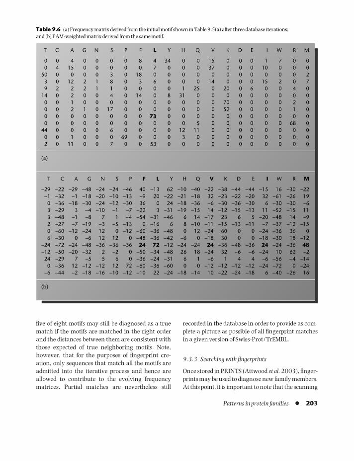
five of eight motifs may still be diagnosed as a truematch if the motifs are matched in the right orderand the distances between them are consistent withthose expected of true neighboring motifs. Note,however, that for the purposes of fingerprint cre-ation, only sequences that match all the motifs areadmitted into the iterative process and hence areallowed to contribute to the evolving frequencymatrices. Partial matches are nevertheless still

recorded in the database in order to provide as com-plete a picture as possible of all fingerprint matchesin a given version of Swiss-Prot/TrEMBL.

9.3.3 Searching with fingerprints

Once stored in PRINTS (Attwood et al. 2003), finger-prints may be used to diagnose new family members.At this point, it is important to note that the scanning

Patterns in protein families l 203

T C A G N S P F L Y H Q V K D E I W R M

0 0 4 0 0 0 0 8 4 34 0 0 15 0 0 0 1 7 0 00 4 15 0 0 0 0 0 7 0 0 0 37 0 0 0 10 0 0 0

50 0 0 0 0 3 0 18 0 0 0 0 0 0 0 0 0 0 0 23 0 12 2 1 8 0 3 6 0 0 0 14 0 0 0 15 2 0 79 2 2 2 1 1 0 0 0 0 1 25 0 20 0 6 0 0 4 0

14 0 2 0 0 4 0 14 0 8 31 0 0 0 0 0 0 0 0 00 0 1 0 0 0 0 0 0 0 0 0 0 70 0 0 0 0 2 00 0 2 1 0 17 0 0 0 0 0 0 0 52 0 0 0 0 1 00 0 0 0 0 0 0 0 73 0 0 0 0 0 0 0 0 0 0 00 0 0 0 0 0 0 0 0 0 0 5 0 0 0 0 0 0 68 0

44 0 0 0 0 6 0 0 0 0 12 11 0 0 0 0 0 0 0 00 0 1 0 0 0 69 0 0 0 3 0 0 0 0 0 0 0 0 02 0 11 0 0 7 0 0 53 0 0 0 0 0 0 0 0 0 0 0

(a)

T C A G N S P F L Y H Q V K D E I W R M

−29 −22 −29 −48 −24 −24 −46 40 −13 62 −10 −40 −22 −38 −44 −44 −15 16 −30 −22−1 −32 −1 −18 −20 −10 −13 −9 20 −22 −21 −18 32 −23 −22 −20 32 −61 −26 190 −36 −18 −30 −24 −12 −30 36 0 24 −18 −36 −6 −30 −36 −30 6 −30 −30 −63 −29 3 −4 −10 −1 −7 −22 3 −31 −19 −15 14 −12 −15 −13 11 −52 −15 113 −48 −1 −8 7 1 −4 −54 −31 −46 6 14 −17 23 6 5 −20 −48 14 −92 −27 −7 −19 −3 −5 −13 0 −16 6 8 −10 −11 −15 −13 −11 −7 −37 −12 −150 −60 −12 −24 12 0 −12 −60 −36 −48 0 12 −24 60 0 0 −24 −36 36 06 −30 0 −6 12 12 0 −48 −36 −42 −6 0 −18 30 0 0 −18 −30 18 −12

−24 −72 −24 −48 −36 −36 −36 24 72 −12 −24 −24 24 −36 −48 −36 24 −24 −36 48−12 −50 −20 −32 2 −2 0 −50 −34 −48 26 18 −24 32 −6 −6 −24 10 62 −224 −29 7 −5 5 6 0 −36 −24 −31 6 1 −6 1 4 4 −6 −56 −4 −140 −36 12 −12 −12 12 72 −60 −36 −60 0 0 −12 −12 −12 −12 −24 −72 0 −24

−6 −44 −2 −18 −16 −10 −12 −10 22 −24 −18 −14 10 −22 −24 −18 6 −40 −26 16

(b)

Table 9.6 (a) Frequency matrix derived from the initial motif shown in Table 9.5(a) after three database iterations; and (b) PAM-weighted matrix derived from the same motif.

BAMC09 09/03/2009 16:39 Page 203

algorithms used to create fingerprints (Parry-Smithand Attwood 1992) and to search against themonce deposited in the database (Scordis, Flower, andAttwood 1999) are rather different. The fingerprint-creation process is deliberately conservative, exploit-ing only observed residue frequencies to generateclean, highly selective discriminators; this is vital, asinadvertent inclusion of false matches would com-promise diagnostic performance. Conversely, toallow a wider diagnostic net to be cast, the finger-print-search method is more permissive; the onus isthen on the user to determine whether a match islikely to be true or not. Here, then, the motifs storedin PRINTS are used to generate (ungapped) profiles,using BLOSUM matrices to boost the matrix scores.The rest of the algorithm is much the same as forfingerprint creation, in so far as motifs are requiredto be matched in the correct order with appropriatedistances between them. However, rather than relyon the rank-ordering of absolute scores in a hit list,

probability (p) and expect (E) values are calculatedboth for individual-motif matches and for multiple-motif matches, giving an overall estimate of the like-lihood of having matched a fingerprint by chance(Scordis, Flower, and Attwood 1999).

Probably the best way of appreciating what itmeans to match a fingerprint is to depict the resultgraphically, as illustrated in Fig. 9.2. Within thegraphs shown, the horizontal axis represents thequery sequence, the vertical axis the percent score of each motif (0–100 per motif ). Using a sliding-window approach, for each motif, a window whosewidth is the width of the motif is moved one residueat a time from N to C terminus, and the profile scorecalculated for each position. Where a high-scoringmatch is made above a predefined threshold(17–20% identity), a block is drawn whose leadingedge marks the first position of the match. Blocksappearing in a systematic order along the sequenceand above the level of noise indicate matches with

204 l Chapter 9

PRION_HUMAN vs. PRION(a) (b) PRION_CHICK vs. PRION

0 253

% S

core

Residue number0 273

Residue number

8

7

6

5

4

3

2

1

Fig. 9.2 Graphs used to visualize protein fingerprints. The horizontal axis represents the query sequence, the vertical axis the %score of each motif (0–100 per motif ), and each block a residue-by-residue match in the sequence, its leading edge marking thefirst position of the match. Solid blocks appearing in a systematic order along the sequence and above the level of noise indicatematches with the constituent motifs. The graphs depict prion fingerprints of the human prion protein (a) and of its chickenhomolog (b). The human prion protein is clearly a true-positive match, containing all eight motifs; the chicken homolog fails tomake a complete match, but can still be identified as a family member because of the diagnostic framework provided by the fivewell-matched motif neighbors.

BAMC09 09/03/2009 16:39 Page 204

each of the constituent motifs. In Fig. 9.2, graphs areplotted for (a) a complete match of the human prionsequence against the prion fingerprint, and (b) a partial, but nevertheless true, match of the chickenprion sequence against the same fingerprint. Here,we can see that even though parts of the signatureare missing (motifs 2, 7, and 8), the chicken isrelated to the human sequence. Inspection of thehuman prion database entry reveals that motifs 2–4reside in the region of the N-terminal octapeptiderepeat. When we compare the chicken sequence,not surprisingly, we find that it is characterized by a modified repeat, which explains why a match to motif 2 is missing, and why the matches to motifs3 and 4 are relatively weak; the sequence also showsconsiderable divergence toward the C terminus,which is why motifs 7 and 8 are missing. Thusfingerprints not only allow the diagnosis of true fam-ily members that match them completely, but alsopermit the identification of partially matching relat-ives, yielding important insights into the differencesbetween them.

9.4 PROFILES AND PSSMS

9.4.1 Blocks

As we have discussed, the scoring system for match-ing the motifs of a fingerprint uses unweightedresidue frequencies and, in situations where fewsequences are available, this may compromise diag-nostic performance. With the signal-to-noise caveatsmentioned in Section 9.3, it is possible to build altern-ative motif representations by applying differentweighting schemes.

One such approach is embodied in the Blocks data-base (Henikoff et al. 2000, Henikoff and Henikoff1994a). Here, conserved motifs, termed blocks, arelocated by searching for spaced residue triplets (e.g., Asn-x-x-Glu-x-x-x-x-x-x-x-x-x-x-Glu, where xrepresents any amino acid). Any redundant blocksgenerated by this process are removed, only thehighest-scoring blocks being retained – block scoresare calculated using the BLOSUM62 substitutionmatrix. The validity of blocks found by this method is confirmed by the application of a second motif-

finding algorithm, which searches for the highest-scoring set of blocks that occur in the correct orderwithout overlapping. Blocks found by both methodsare considered reliable and are stored in the databaseas ungapped local alignments. These are then calib-rated against Swiss-Prot to obtain a measure of thelikelihood of a chance match. Two scores are notedfor each block: one denotes the score above which amatch is likely to be significant (the median true-positive score); the other denotes the score belowwhich a match is probably spurious (the 99.5th per-centile of true-negative scores). The ratio of thesecalibration scores multiplied by 1000 is referred toas the block strength, which allows the diagnosticperformance of individual blocks to be meaningfullycompared (Henikoff and Henikoff 1991, 1994b).

A typical block is illustrated in Fig. 9.3. Sequencesegments within the block are clustered to reducemultiple contributions to residue frequencies fromgroups of closely related sequences. This is particu-larly important for deep motifs (i.e., with contribu-tions from tens or hundreds of sequences), whichcan be dominated by numerous virtually identicalsequences. Each cluster is then treated as a singlesegment, each of which is assigned a score that givesa measure of its relatedness. The higher the weight,the more dissimilar the segment is from other seg-ments in the block; the most distant segment is givena weight of 100.

9.4.2 Searching with blocks

As with fingerprinting, blocks may be used to detectadditional family members in sequence databases.In a manner reminiscent of fingerprint searches,blocks are converted to position-specific substitutionmatrices, which are used to make independentdatabase searches. The results are compared and,where several blocks detect the same sequence, an E value is calculated for the multiple hit. Clearly, themore blocks matched, the greater the confidencethat the sequence is a family member. However, as with all weighting schemes, there is a diagnostictrade-off between the ability to capture all true family members with a block or set of blocks, and the likelihood of making false matches. Unless a

Patterns in protein families l 205

BAMC09 09/03/2009 16:39 Page 205

family is characterized by only one block, individualblock matches are not usually biologically signific-ant; multiple-block matches are much more likely tobe real, provided the blocks are matched in the cor-rect order and have appropriate distances betweenthem.

The information content of blocks can be visual-ized by examination of their so-called sequence logos(Plate 9.1(a)). A logo is a graphical display of analigned motif, consisting of color-coded stacks of let-ters representing the amino acid residues at eachposition in the motif. Letter height increases with

increasing frequency of the residue, such that themost conserved positions have the tallest letters.Within stacks, the most frequently occurring re-sidues also occupy the highest positions, so that themost prominent residue, at the top of the stack, is the one most likely to occur at that position. Toreduce bias resulting from sequence redundancywithin blocks, weights are calculated using a PSSM.This reduces the tendency for over-representedsequences to dominate stacks, and increases the representation of rare amino acid residues relative to common ones. The logo calculated for the prion

206 l Chapter 9

Fig. 9.3 Block for the prion proteinfamily, in which sequence segments areclustered and weighted according totheir relatedness – the most distantsequence within the block scores 100(for convenience, part of the block hasbeen deleted, as denoted by . . . ).

BAMC09 09/03/2009 16:39 Page 206

block depicted in Fig. 9.3 is illustrated in Plate9.1(a). The highly conserved anchor triplet, GPG, isclearly visible toward the center of the logo.

9.4.3 Profiles

By contrast with motif-based pattern-recognitiontechniques, an alternative approach is to distil thesequence information within complete alignmentsinto scoring tables, or profiles (Gribskov, McLachlan,and Eisenberg 1987, Bucher and Bairoch 1994). A profile can be thought of as an alternating sequ-

ence of “match” and “insert” positions that containscores reflecting the degree of conservation at eachalignment position. The scoring system is intricate:as well as evolutionary weights (e.g., PAM scores), itincludes variable penalties to weight against inser-tions and deletions occurring within core secondarystructure elements; match, insertion, and deletionextension penalties; and state transition scores.

Part of a typical profile is illustrated in Fig. 9.4.Position-specific scores for insert and match statesare contained in /I and /M fields respectively. Thesetake the form:

Patterns in protein families l 207

Fig. 9.4 Example PROSITE profile,showing position-specific scores forinsert and match positions. Penaltieswithin insert positions are highlightedbold: here, the values are more tolerantof indels by comparison with the largeoverall penalties set by the DEFAULTparameter line.

BAMC09 09/03/2009 16:39 Page 207

/I: [SY=char1; parameters;]

/M: [SY=char2; parameters;]

where char1 is a symbol that represents an insertposition in the parent alignment; char2 is a symbolthat represents a match position in the parent align-ment; and parameters is a list of specificationsassigning values to various position-specific scores(these include initiation and termination scores,state transition scores, insertion/match/deletionextension scores, and so on).

In the example shown in Fig. 9.4, the sequencecan be read off from the successive /M positions: F-I-A-L-Y-D, etc. It is evident that the profile containsthree conserved blocks separated by two gappedregions. Within the conserved blocks, small inser-tions and deletions are not totally forbidden, but arestrongly impeded by large gap penalties defined inthe DEFAULT data block: MI=-26, I=-3, MD=-26,D=-3 (MI is a match-insert transition score, I is aninsert extension score, MD is a match-delete transi-tion score, and D is a deletion extension score). Thesepenalties are superseded by more permissive valuesin the two gapped regions (e.g., in the first of these,MI=0, I=-1, MD=0, etc.).

The inherent complexity of profiles renders themhighly potent discriminators. They are thereforeused to complement some of the poorer regexs inPROSITE, and/or to provide a diagnostic alternativewhere extreme sequence divergence renders the useof regexs inappropriate. Before finishing this sectionon profile methods, we note that PSI-BLAST, whichwe already discussed in Chapter 7, can also beclassed as a profile method, as it builds up a PSSMbased on the first BLAST search, and uses this to per-form further searches.

9.5 BIOLOGICAL APPLICATIONS – GPROTEIN-COUPLED RECEPTORS

9.5.1 What are G protein-coupled receptors?

The best way to try to understand the range of pattern-recognition methods described in this chap-ter is to consider how they have been applied to real biological examples. To this end, the following

sections concern the analysis of G protein-coupledreceptors, comparing and contrasting the results ofusing pairwise and family-based search tools, andexamining the biological insights that each of theseapproaches affords.

G protein-coupled receptors (GPCRs) constitute a large, functionally diverse and evolutionarily tri-umphant group of cell-surface proteins (Teller et al.2001). They are involved in an incredible range ofphysiological processes, adapting a common struc-tural framework to mediate, for example, vision,olfaction, chemotaxis, stimulation and regulation ofmitosis, and the opportunistic entry of viruses intocells (Lefkowitz 2000, Hall, Premont, and Lefkowitz1999). This functional diversity is achieved viainteractions with a wide variety of ligands (includingpeptides, glycoproteins, small molecule messengermolecules (such as adrenaline), and vitamin derivat-ives (such as retinal)), the effects of which stimulatea range of intracellular pathways through couplingto different guanine nucleotide-binding (G) proteins.

9.5.2 Where did GPCRs come from?

How did this extraordinary functional versatilityarise? The GPCRs we see in modern organisms arepart of a vast multi-gene family, which is thought to have diverged from an ancient ancestral mem-brane protein. Details of the origins of GPCRs are still contentious, but clues are perhaps to be found in the bacterial opsins. The bacterial opsins are reti-nal-binding proteins that provide light-dependention transport and sensory functions to a family ofhalophilic bacteria. They are integral membraneproteins that contain seven transmembrane (TM)domains, the last of which contains the chromophoreattachment point. There are several classes of thisbacterial protein, including bacteriorhodopsin andarchaerhodopsin, which are light-driven protonpumps; halorhodopsin, a light-driven chloride pump;and sensory rhodopsin, which mediates both photo-attractant (in the red) and photophobic (in the UV)responses.

From an evolutionary perspective, two features ofbacterial opsins are particularly interesting. First, theprotein has a 7TM architecture (bacteriorhodopsin

208 l Chapter 9

BAMC09 09/03/2009 16:39 Page 208

was the first membrane protein whose structure wasdetermined at atomic resolution (Henderson et al.1990, Pebay-Peyroula et al. 1997)); second, itsresponse to light is mediated by retinal (a vitamin Aderivative), which is bound to the protein via alysine residue in the seventh TM domain. There arestriking parallels here with the protein rhodopsin, aGPCR that plays a central role in light reception inhigher organisms. For a long time, the architectureof rhodopsin was believed to be like that of bacterio-rhodopsin, with 7TM helices snaking back and forthacross the membrane (NB, GPCRs are sometimesreferred to as “serpentine” receptors). Indeed, sogreat was the confidence in their structural similar-ity that almost all of the early models of the structure of rhodopsin were based on the bacteriorhodopsintemplate. The crystal structure of bovine rhodopsinwas solved relatively recently (Palczewski et al. 2000),and confirmed both the 7TM architecture and thelocation of its bound chromophore, retinal, which isattached via a Schiff ’s base to a lysine residue in theseventh TM domain.

In spite of these striking similarities, however,there are also significant differences. First, bacterio-rhodopsin does not couple to G proteins. Second,there is no significant sequence similarity betweenrhodopsin and bacteriorhodopsin, beyond the gen-eral hydrophobic nature of the TM domains and theretinal-attachment site. Third, the rhodopsin cry-stal structure highlighted important differences inthe packing of its helices relative to that seen in bacteriorhodopsin, rendering many of the earlyhomology models virtually worthless. In light of theobvious similarities and differences between them, it therefore remains unclear whether the 7TM architecture was recruited by the GPCRs from thebacterial opsins and adapted to fulfil many differentfunctional roles, or whether nature invented the7TM framework more than once to confer transportand sensory functions on its host cells – withoutsignificant sequence similarity, we can neither con-firm homology nor rule out analogy. Consequently,the optimistic researchers who modeled rhodopsinby homology with bacteriorhodopsin learned somepainful lessons about the dangers of overinterpret-ing data and about the importance of understanding

the evolutionary origins of the molecules we areinvestigating.

9.5.3 GPCR orthologs and paralogs

If the ancient origins of GPCRs are unclear, theirmore recent history is somewhat better understood(partly because many GPCRs share a high degree ofsequence similarity and partly because, today, wehave an abundance of sequence information onwhich to perform comparative or phylogenetic ana-lyses). GPCRs have successfully propagated through-out the course of evolution both by speciation events(orthology) and via gene-duplication events withinthe same organism (paralogy). It is beyond the scopeof this chapter to provide a detailed discussion of allGPCRs, but we will focus for a moment on one of thefamilies in order to highlight the challenges thatbiology presents to the bioinformatician. We will dothis by taking a closer look at rhodopsin, because itwas one of the first GPCRs to be studied in detail andthe largest GPCR superfamily is named after it – therhodopsin-like GPCRs.

As already mentioned, rhodopsin is a light recep-tor. It resides in the disk membranes of retinal rodcells and functions optimally in dim light. Animalsthat depend on good night vision (cats, for example,which hunt by night) have large numbers ofrhodopsin-harboring rods in their retinas. By con-trast, the visual machinery of some animals is optim-ized for bright light; the retinas of these animals are packed with greater numbers of cone cells –these contain the blue-, red-, and green-pigmentproteins termed opsins. Opsins and rhodopsins share~40% sequence identity and are believed to haveevolved from an ancestral visual pigment via a seriesof gene-duplication events. The duplication thatgave rise to the distinct red- and green-sensitive pig-ment genes is considered to be relatively recentbecause the DNA sequences of the red and greengenes share ~98% sequence identity, suggestingthat there has been little time for change. This obser-vation finds support in comparisons of the distribu-tion of visual genes in new- and old-world monkeys:new-world monkeys have only a single visual-pigment gene on the X chromosome; by contrast,

Patterns in protein families l 209

BAMC09 09/03/2009 16:39 Page 209

old-world monkeys have two X-chromosome visualpigment genes (similarly, in humans, the red- andgreen-sensitive genes lie on the X chromosome).Thus, the addition of the second X-chromosomegene must have occurred some time after the separa-tion of the new and old world monkeys, around 40million years ago (Nathans 1989).

The location of the red- and green-pigment geneson the X chromosome has long been known tounderpin red–green color blindness. Males will havevariant red–green discrimination if their single Xchromosome carries the trait; females will beaffected only if they receive a variant X chromosomefrom both parents. In fact, males normally have a single copy of the red-pigment gene but one, two,or three copies of the green-pigment gene. Differenttypes of abnormal red–green color discriminationthen arise from genetic exchanges that result in the loss of a pigment gene or the creation of part-red/part-green hybrid genes (Nathans 1989).

So, to recap, an ancestral visual pigment has givenrise to the rhodopsin family. In vertebrates, the family includes an achromatic receptor (rhodopsin)and four chromatic paralogs (the purple, blue, red,and green opsins). In humans, the gene for the greenreceptor may occur in different copy numbers – distorted color perception occurs when the numbersand types of these genes present in an individual areaberrant. The opsins and rhodopsin share a highdegree of sequence similarity, with greatest similar-ity between the red and green pigment proteins; andthe proteins are also highly similar to orthologs indifferent species. If we are interested in sequenceanalysis, this seems like a fairly straightforward scen-ario. However, the family holds further layers ofcomplexity and its analysis requires careful thought.Although, as we might expect, most rhodopsinshave a typical “rhodopsin-like” sequence and mostopsins have typical “pigment-like” sequences, thereare exceptions – thus, for example, green opsins ofthe goldfish, chicken, and blind cave fish moreclosely resemble the canonical rhodopsin sequencethan they do other green sequences. Likewise, blueopsins of the gecko and green chameleon are moresimilar to rhodopsin sequences than to other bluesequences. These unusual sequence relationships

are illustrated in Plate 9.1(b) and (c). Unravelingthis kind of relationship, where a protein with particular biological attributes has the “wrong”sequence, using naïve search tools can thereforelead to erroneous conclusions. Nevertheless, it isprecisely this kind of anomaly that helps to shedlight on the evolutionary ancestry of protein fam-ilies: in this example, the results suggest, perhapssurprisingly, that the gene for achromatic (scotopic)vision (rhodopsin) evolved out of those for color(photopic) vision (opsins) (Okano et al. 1992).

9.5.4 Why GPCRs are interesting and howbioinformatics can help to study them

As we have seen, the long evolutionary history ofGPCRs has generated considerable complexity forjust one of its gene families. Now consider that thereare over 800 GPCR genes in the human genome.These fall into three major superfamilies (termedrhodopsin-, secretin-, and metabotropic glutamatereceptor-like), which are populated by more than 50 families and 350 receptor subtypes (Takeda et al.2002, Foord 2002, Attwood 2001); members of thedifferent superfamilies share almost no recognizablesequence similarity, but are united by the familiar7TM architecture. The receptors are activated by different ligands, some of which are bound in theexternal loop regions, others being bound within theTM scaffold – the opsins are unusual in being covalently attached to their retinal chromophore.The activated receptors then interact with differentG proteins or other intracellular molecules to effecttheir diverse biological responses. The extent of thefamily, the richness of their evolutionary relation-ships, and the complexity of their interactions withother molecules are not only challenging to under-stand, but are also very difficult to analyze computa-tionally. If we wish to derive deeper insights into theways in which genomes encode biological functions,our traditional pairwise similarity search tools arelikely to be limited. These tools have been the main-stays of genome annotation endeavors because theyreduce a complex problem to a more tractable one –that of identifying and quantifying relationshipsbetween sequences. But identifying relationships

210 l Chapter 9

BAMC09 09/03/2009 16:39 Page 210

between sequences is clearly not the same as identi-fying their functions, and failure to appreciate thisfundamental point has generated numerous anno-tation errors in our databases.

Interest in GPCRs reaches beyond mere academicintrigue and the desire to place them into func-tionally related families. The receptors are also ofprofound medical importance, being involved in several major pathophysiological conditions, includ-ing cardiovascular disease, cancer, and pathologicalirregularities in body weight homeostasis. The pivotal role of GPCRs in regulating crucial cellularprocesses, and the diseases that arise when these processes go wrong, has placed them firmly in thepharmaceutical spotlight, to such an extent that,today, they are the targets of the majority of pre-scription drugs: more than 50% of marketed drugsact at GPCRs (including a quarter of the 100 top-selling drugs), yielding sales in excess of US$16 billion per annum (Flower 1999). GPCRs are there-fore “big business”.

Nevertheless, there is still only one crystal struc-ture available to date (their membranous locationrenders GPCRs largely intractable to conventionalcrystallographic techniques). Moreover, the hugenumbers of receptors have defied our ability to characterize them all experimentally. Consequently,many remain “orphans”, with unknown ligand spe-cificity. In the absence of experimental data, bioin-formatics approaches are therefore often used to helpidentify, characterize, and model novel receptors(Gaulton and Attwood 2003, Attwood and Flower2002): e.g., if a receptor is found to share significantsequence similarity with one of known function, itmay be possible to extrapolate certain functional andstructural characteristics to the uncharacterizedprotein. Bioinformatics approaches are thereforeimportant in the ongoing analysis of GPCRs, offeringcomplementary tools with which to shed light on thestructures and functions of novel receptors, and thehope of discovering new drug targets.

9.5.5 Detecting sequence similarity

We have already seen in Chapter 7 that the fastestand most frequently used method for identifying sets

of sequences related to a query is to search sequencedatabases using pairwise alignment tools such asBLAST and FASTA (Altschul, Gish, and Miller 1990,Altschul et al. 1997, Pearson and Lipman 1988,Pearson 2000). Several novel GPCRs have beenidentified in this way as a result of their similarity toknown receptors (Takeda et al. 2002, Lee et al. 2001,Radford, Davies, and Dow 2002, Hewes and Taghert2001, Zozulya, Echeverri, and Nguyen 2001).

However, pairwise alignment/search tools havevarious inherent problems, not least that differentprograms often return different results (to be rigor-ous, BLAST and FASTA should be used together, asthey give different perspectives on the same query,often yielding different top hits). These programs areconsequently limited when it comes to the moreexacting tasks of identifying the precise families towhich receptors belong and the ligands they bind.The problem is, it is difficult to determine at whatlevel of sequence identity ligand specificity will beconserved: some GPCRs, with as little as 25% ident-ity, share a common ligand (e.g., the histaminereceptors); others, with greater levels of identity, donot (e.g., receptors for melanocortin, lysophosphat-idic acid, and sphingosine 1-phosphate). Thus, it isoften impossible to tell from a BLAST result whetheran orphan receptor is likely to be a member of aknown family, to which it is a top hit, or whether itwill bind a novel ligand. Consider, for example, therecently de-orphaned urotensin II receptor: BLASTindicates that it is most similar to the type 4 somato-statin receptors, yet it is now known to bind a dif-ferent (though related) ligand (Fig. 9.5). Thus, it is clearly a dangerous (though all too common)assumption that the top most statistically significanthit is also the most biologically relevant.

9.5.6 Diagnosing family membership

Earlier in this chapter, we discussed how searchmethods based on alignments of protein familieshave evolved to address some of the problems of pairwise approaches, and these have given rise to arange of family databases, as outlined in Chapter 5.The principle underlying such methods is that by aligning representative family members, it is

Patterns in protein families l 211

BAMC09 09/03/2009 16:39 Page 211

possible to identify conserved regions (whether short“motifs” or complete domains) that are likely to havecritical structural or functional roles. These regionsmay then be used to build diagnostic signatures,with enhanced selectivity and sensitivity, allowingnew family members to be detected more reliably.

As we have seen, the family-based approaches differ both in terms of the extent of the alignmentthey use and in the methods used to encode con-served regions (recall Fig. 5.6). The main techniquesuse: (i) single conserved regions encoded as regexs(as in PROSITE (Falquet et al. 2002) and eMOTIF(Huang and Brutlag 2001)); (ii) multiple motifsencoded as fingerprints (as in PRINTS (Attwood et al.2003)) or sets of blocks (in Blocks (Henikoff et al.2000)); or (iii) complete domains encoded as profiles(Gribskov et al. 1987, Bucher and Bairoch 1994) (as in PROSITE (Falquet et al. 2002)) or HMMs(Krogh et al. 1994, Eddy 1998) (as in Pfam(Bateman et al. 2002)).

These different approaches have different diag-nostic strengths and weaknesses, which must beunderstood when applying them. For example,regexs have to be matched exactly, which often

leads to high error rates: many true relationships aremissed because sequences deviate slightly from theexpression, and many false matches are madebecause the patterns are short and non-selective.With fingerprints, although individual motifs maybe relatively short, greater selectivity is achieved byexploiting the mutual context of motif neighbors – false-positive matches can then be more easily dis-tinguished from true family members, as they usu-ally fail to match most of the motifs within a givenfingerprint. However, as no weighting scheme isused to derive fingerprints, those that encode super-families may be too selective and consequently maymiss true family members. By contrast, the scoringmethods used in the derivation of Blocks exploitweighted PSSMs, rather than the frequency mat-rices typical of fingerprinting – this may have theeffect not only of boosting weak biological signals,but also of upweighting spurious matches. More-over, blocks are automatically derived and theirnumbers and diagnostic potential often differ fromequivalent fingerprints, often causing confusionamong users. On the other hand, both profiles andHMMs perform well in the diagnosis of distant family

212 l Chapter 9

Fig. 9.5 BLAST output from a search of Swiss-Prot (release 40.29) with the human urotensin II receptor sequence(UR2R_HUMAN, Q9UKP6). Note, there is no clear cut-off between the urotensin, somatostatin, and galanin receptor matches.

BAMC09 09/03/2009 16:39 Page 212

members of large divergent superfamilies but, unlikefingerprints, rarely offer the means to diagnose sequ-ences at the level of families or subfamilies (they mayalso be prone to profile dilution if they have beenderived by purely automatic means).

To simplify sequence analysis, many of these data-bases have been integrated into InterPro (Mulder et al. 2003), which amalgamates their family documentation into a coherent whole, and allowsmultiple repositories to be searched simultaneously.In the following section, we will consider howInterPro and its constituent databases can be used toshed light on features of GPCR sequences. In particu-lar, we draw attention to the different perspectivesoffered by their search tools, and discuss the import-ance this is likely to have when diagnosing novelsequences and attempting to make predictionsabout likely ligand specificity or G protein coupling.

9.5.7 Analysis of GPCRs

The databases described above all provide signat-ures for GPCRs. PROSITE contains regexs for thethree major superfamilies. The expressions are relat-ively short, and cover N-terminal regions or parts ofthe TM domains. The database also contains a singlefamily-level expression, for the opsins. The error rateassociated with these signatures is high. The expres-sion-encoding TM domain 3 of the rhodopsin-likesuperfamily, for example, fails to detect more than100 known superfamily members, including thehuman P2Y6, UDP-glucose, NPY5, and PAR2receptors. These sequences are annotated as false-negatives, but many additional sequences, such asthe KiSS-1 receptor and the orphan SALPR (somato-statin and angiotensin-like peptide receptor), fail tomatch and are not recorded in the documentation.The actual error rate is therefore considerably higherthan it first appears (Gaulton and Attwood 2003).

PROSITE also contains profiles encoding the 7TMregions of each of the GPCR superfamilies; these perform better, with few or no false-positives andfalse-negatives recorded. Similarly, Pfam contains7TM-encoding HMMs for each of the superfamilies,which perform well and detect distant family mem-bers missed by regexs. Both databases also provide

discriminators for the N-terminal domain of thesecretin receptor-like superfamily.

These signatures are useful diagnostic tools thatcan help to identify putative GPCRs, and many havebeen used to search recently sequenced genomes(Brody and Cravchik 2000, Remm and Sonnhammer2000). However, as there is only a single signatureat the family level (the PROSITE expression foropsin), searches with this sort of signature offer vir-tually no opportunity to identify the family to whichan orphan receptor might belong, to predict the type of ligand it might bind, or to predict the type of Gprotein to which it might couple. In trying to charac-terize a putative GPCR, it is not enough to say thatthe sequence might be a rhodopsin-like receptor,because this does not tell us of which of the possible~50 families it is a member (and hence its ligand-binding specificity), and which of the family sub-types it most closely resembles (and hence its likely Gprotein-coupling preference).

PRINTS contains the most extensive collection ofGPCR signatures of any family database, with morethan 270 fingerprints (Attwood, Croning, andGaulton 2002). The nature of the analysis method ituses means that highly selective fingerprints can becreated in a hierarchical manner for receptor super-families, families, and subtypes. Therefore, searches ofthis resource may not only identify the superfamilyto which a receptor belongs, but may also elucidateits family and subtype relationships (see Fig. 9.6).

The ability of fingerprints to distinguish betweenclosely related receptor families and subtypes is illus-trated in Fig. 9.7. Here, the sequence of the humanurotensin II receptor was searched against (a) itsown fingerprint and (b) the somatostatin receptorfamily fingerprint (Gaulton and Attwood 2003).Recall Fig. 9.5, in which the BLAST search could notclearly distinguish the urotensin II receptor from the somatostatin receptors. Here, by contrast, thePRINTS result clearly highlights the differencesbetween them – the receptor perfectly matches itsown fingerprint (each motif matched is indicated bya block on the graph), but fails to match any of themotifs that characterize the somatostatin receptors.This is important. The result reflects the fact that al-though the urotensin II and somatostatin receptors

Patterns in protein families l 213

BAMC09 09/03/2009 16:39 Page 213

PF00001

Rhodopsin-like GPCR superfamily

PR00896

Vasopressin receptor

PR00752

Vasopressin V1A receptor

PS50262

PS00237

PR00237

7tm_1

VASOPRESSINR

VASOPRSNV1AR

G_PROTEIN_RECEP_F1_2

G_PROTEIN_RECEP_F1_1

GPCRRHODOPSN

Fig. 9.6 Output from a search of InterPro with the human vasopressin 1A receptor sequence (V1AR_HUMAN). The receptormatches the Pfam HMM (PF00001 – white bar), PRINTS fingerprint (PR00237 – black bars), and PROSITE regular expression(PS00237 – spotted bar) and profile (PS50262 – striped bar) for the rhodopsin-like superfamily of GPCRs. However, only PRINTSgives family- and subtype-level diagnoses, with matches to the vasopressin receptor family (PR00896) and vasopressin V1Areceptor subtype (PR00752) fingerprints.

UR2R_HUMAN vs. UROTENSIN2R(a) (b) UR2R_HUMAN vs. SOMATOSTANR

1 380

% ID

Residue number1 380

Residue number

8

9

7

6

5

4

3

2

1

7

6

5

4

3

2

1

Fig. 9.7 Output from a search of the human urotensin II receptor sequence against (a) its own fingerprint and (b) thesomatostatin receptor family fingerprint using PRINTS’ GRAPHScan tool (Scordis, Flower, and Attwood 1999). Within eachgraph, the horizontal axis represents the sequence, and the vertical axis the percentage score (identity) of each fingerprint element(0–100 per motif ). Filled blocks mark the positions of motif matches above a 20% threshold. Here, we see that the receptor matchesall nine motifs of its own fingerprint but fails to make any significant matches to the somatostatin receptor fingerprint.

BAMC09 09/03/2009 16:39 Page 214

share a high degree of overall similarity (this is whatBLAST “sees”), they differ in key regions that arelikely to determine their functional specificity (i.e.,what fingerprints “see”). Thus, BLAST, FASTA, andsuperfamily-level discriminators operate at a gen-eric similarity level, while fingerprints provide muchmore fine-grained insights based on both the similar-ities and the differences between closely relatedsequences.

Several other methods have also been developedfor classifying GPCRs, including those that use sup-port vector machines, phylogenetic analysis, andanalysis of receptor chemical properties. These willnot be discussed further here, but interested readersare referred to Joost and Methner (2002), Karchin,Karplus, and Haussler (2002), and Lapinsh et al.(2002).

9.5.8 The functional significance of signatures

Although most protein family signatures are derivedsolely on the basis of amino acid conservation, with-out explicit consideration of function, it is evidentthat the conserved regions they exploit do cor-respond to structural and functional motifs. Forexample, at the superfamily level, all GPCRs sharethe same architecture; consequently, the superfam-ily signatures primarily encode the 7TM domains(which makes sense, because this is what they allhave in common). If we think about individual fam-ilies within a particular GPCR superfamily, however,what are the defining characteristics? The 7TMarchitecture is the same, isn’t it, so what makes anopsin sequence different from an olfactory receptorsequence, and different again from a muscarinicreceptor sequence, and so on? If the structure is thesame, we can reasonably suppose that the differencebetween them must lie in the way the differentreceptors function – i.e., in the ligands they bind.Detailed analyses of the fingerprints that define thedifferent GPCR families suggest that this is the case:motifs of family-level fingerprints are often found inparts of the TM domains and extracellular portionsof the receptors, reflecting the regions in which theybind a common ligand. But what of individual recep-tor subtypes? These not only share the same struc-

ture, but also bind the same ligand as their siblingsubtypes, so what makes them different? In this case,we conclude that the defining characteristics are intheir G protein-coupling preferences (whether Gi,Go, Gq, etc.). Once again, examination of subtypefingerprints indicates that the constituent motifs aremore prevalent in intracellular regions, particularlythe third intracellular loop and C-terminal regions,most likely to be involved in G protein coupling.

Reassuringly, in the case of family-level finger-prints, experimental evidence is beginning to confirmtheir functional significance: residues shown bymutational or molecular modeling studies to be in-volved in ligand binding often fall within the motifsthat characterize the family. In addition, recentmodeling studies have predicted 3D structures forthe sphingosine 1-phosphate (S1P) receptors EDG1and EDG6, and identified residues likely to beinvolved in binding the ligand (Parrill et al. 2000,Wang et al. 2001, Vaidehi et al. 2002). Figure 9.8

Patterns in protein families l 215

N

C

5 6 721 3 4

Fig. 9.8 Schematic diagram representing the endothelialdifferentiation gene (EDG) family of sphingosine 1-phosphatereceptors. Positions of the fingerprint motifs for this family are indicated by rectangles; circles mark the positions ofresidues known to be important in ligand binding in the EDG1receptor (black) (Remm and Sonnhammer 2000, Attwood et al.2002) and in the EDG6 receptor (white) ( Joost and Methner2002). Models of these receptors predict that the ligand bindswithin the TM regions, close to domains 2, 3, 5, and 7.

BAMC09 09/03/2009 16:39 Page 215

shows a schematic diagram of an S1P receptor, withthe positions of these critical residues indicated byasterisks, and motifs of the family fingerprint indic-ated by shaded boxes; all of the ligand-bindingresidues identified to date lie within two of the motifs(Gaulton and Attwood 2003). Moreover, the re-maining motifs lie in regions that appear to be closeto the ligand-binding site (TM domains 2, 3, 5, and

7), or in regions that may be involved in G proteincoupling, reflecting the overlapping coupling specific-ity of receptors in this family. These results highlightthe fact that, in addition to facilitating classificationof orphan receptors, fingerprints may also providevital information about residues and regions ofreceptors that are likely to have crucial functionalroles.

216 l Chapter 9

SUMMARYSearch tools based on pairwise alignment (BLAST andFASTA) have become the methods of choice for manyresearchers – they are quick and easy to use. To quantifythe similarity between matched sequences, the methodsuse different scoring schemes (PAM or BLOSUM), butmatched residue pairs all carry equal weight along thesequence according to the values in the chosen scoringmatrix. In searches for highly divergent sequences, suchtools may lack sensitivity, failing to retrieve true matchesfrom the “twilight zone”. Conversely, in searches forclosely related sequences, they may lack selectivity – itmay be difficult to determine, merely on the basis of an Evalue, whether a matched sequence is a true functionalequivalent (the distinction between orthologs and para-logs may not be clear).

To improve the sensitivity and selectivity of databasesearches, family-based methods were developed. Theinnovation was to use information from multiply alignedsequences to increase the diagnostic potential of sear-ches. The methods still largely use scoring matrices toquantify residue matches, but benefit from the addi-tional residue information stored in each column of thealigned sequences. This is important, because the align-ment tells us which residues are the most conserved –the residues therefore carry position-specific weights,according to the degree of conservation of each align-ment column. The use of multiple sequences thereforeallows PSSMs to be developed to capture the evolution-ary essence of a given protein family.

Different methods have been developed to encodethe conserved information in sequence alignments,using this both to characterize protein families and todiagnose new family members. The methods exploit single motifs, multiple motifs, or complete domains.

Single-motif methods often use regexs to encapsulatethe conserved residues or residue groups from the mostconserved region of an alignment, but these tend to lackdiagnostic power. Family-specific regexs were first usedto create PROSITE. The database also includes non-

family-specific rules, very short regexs that describe func-tional sites, such as glycosylation sites, phosphorylationsites, etc. Rules are not diagnostic – they only indicatethat certain residues exist in a sequence, but not thatthey are functional. To enhance the diagnostic perform-ance of regexs, degrees of variability may be built intoexpressions by tolerating substitutions according to phy-sicochemically based residue groupings. Such regexs arethe basis of eMOTIF.

Multiple-motif methods exploit the fact that mostalignments contain more than one conserved region,and were first used in the fingerprint method that under-pins PRINTS. Motifs are converted to (position-specific)residue frequency matrices, but no additional weightingscheme is used to enhance the scores. The method gainsdiagnostic potency from the biological context affordedby matching motif neighbors, so a sequence can still bediagnosed as a likely family member even if parts of thesignature are absent. However, fingerprints may lackdiagnostic power if derived from protein families withonly few members. To overcome this problem, weight-ing schemes were introduced, leading to the concept ofblocks, the basis of the Blocks database. The potentialdisadvantage of weighted blocks is that the scoringscheme may introduce noise. PRINTS is also available in Blocks format, in which PRINTS’ raw motifs are converted to weighted blocks; PRINTS’ motifs are alsoused to form permissive regexs as part of the eMOTIFresource. The fingerprint approach therefore underpinsmany different diagnostic procedures. A further strengthof the method is that it is not confined to the diagnosisof members of divergent superfamilies: because themethod is selective, it has also been used to distinguishfamilies from their constituent superfamilies, and sub-families from their parent families. No other methodoffers such a hierarchical discriminatory framework.

Profile methods encode both conserved and gappedregions, and exploit position-specific scores and sub-stitution matrices to enhance diagnostic performance.In seeking divergent members of large superfamilies,

BAMC09 09/03/2009 16:39 Page 216

REFERENCESAltschul, S.F., Gish, W., and Miller, W. 1990. Basic local

alignment search tool. Journal of Molecular Biology, 215:403–10.

Altschul, S.F., Madden, T.L., Schaffer, A.A., Zhang, J.,Zhang, Z., Miller, W., and Lipman, D.J. 1997. GappedBLAST and PSI-BLAST: A new generation of proteindatabase search programs. Nucleic Acids Research, 25:3389–402.

Attwood, T.K. 2000a. The quest to deduce protein func-tion from sequence: The role of pattern databases.International Journal of Biochemistry and Cell Biology,32(2): 139–55.

Attwood, T.K. 2000b. The role of pattern databases insequence analysis. Briefings in Bioinformatics, 1: 45–59.

Attwood, T.K. 2001. A compendium of specific motifs fordiagnosing GPCR subtypes. Trends in PharmacologicalSciences, 22(4): 162–5.

Attwood, T.K., Blythe, M.J., Flower, D.R., Gaulton, A.,Mabey, J.E., Maudling, N., McGregor, L., Mitchell, A.L.,Moulton, G., Paine, K., and Scordis, P. 2003. PRINTSand PRINTS-S shed light on protein ancestry. NucleicAcids Research, 30: 239–41.

Attwood, T.K., Croning, M.D., and Gaulton, A. 2002.Deriving structural and functional insights from a

ligand-based hierarchical classification of G protein-coupled receptors. Protein Engineering, 15: 7–12.

Attwood, T.K., Eliopoulos, E.E., and Findlay, J.B.C. 1991.Multiple sequence alignment of protein families show-ing low sequence homology: A methodologicalapproach using pattern-matching discriminators for G-protein linked receptors. Gene, 98: 153–9.

Attwood, T.K. and Findlay, J.B.C. 1993. Design of a dis-criminating fingerprint for G-protein-coupled receptors.Protein Engineering, 6(2): 167–76.

Attwood, T.K. and Flower, D.R. 2002. Trawling the gen-ome for G protein-coupled receptors: The importance of integrating bioinformatic approaches. In Darren R.Flower (ed.), Drug Design – Cutting Edge Approaches,pp.60–71. London: Royal Society of Chemistry.

Bateman, A., Birney, E., Cerruti, L., Durbin, R., Etwiller, L.,Eddy, S.R., Griffiths-Jones, S., Howe, K.L., Marshall, M.,and Sonnhammer, E.L. 2002. The Pfam protein familiesdatabase. Nucleic Acids Research, 30: 276–80.

Benson, D.A., Karsch-Mizrachi, I., Lipman, D.J., Ostell, J.,and Wheeler, D.L. 2004. GenBank: Update. NucleicAcids Research, 32: D23–6.

Brody, T. and Cravchik, A. 2000. Drosophila melanogasterG protein-coupled receptors. Journal of Cell Biology, 150:F83–8.

Patterns in protein families l 217

they tend to be diagnostically more potent than regexs,fingerprints, and blocks; consequently, many are in-cluded in PROSITE. In deriving profiles, care must betaken not to include false family members, as this willlead to profile dilution.

These software tools and databases have been used inthe computational analysis of many different proteinfamilies, and the GPCRs provide a good illustration ofthe relative merits of each. The family-based methodsare particularly valuable in helping to characterize novelreceptors and, in some cases, may allow identification of functional motifs responsible for binding ligands or Gproteins.

Nevertheless, in studying complex gene families, it isimportant to appreciate the limitations of the particu-lar computational methods being applied. No method is infallible and none can replace the need for biolo-gical experimentation and validation. Best results areobtained by using all the available resources and under-standing the problems associated with each. Regexs aregood at detecting short functional motifs. PROSITE

offers a regex for the rhodopsin-like GPCR superfamilyand another for the retinal attachment site of opsins.Profiles and HMMs are good at detecting generic sim-ilarities between divergent members of large superfam-ilies. Superfamily-level profiles and HMMs are availablefrom PROSITE and Pfam. Fingerprints are good at distin-guishing members of functionally related families andsubfamilies. PRINTS offers over 270 fingerprints for therhodopsin-like GPCR families and receptor subtypes; itthus offers more fine-grained diagnoses, providing theopportunity not only to determine the superfamily towhich a GPCR might belong, but also to identify the par-ticular family of which it is a member, and the specificreceptor subtype it most resembles, hence offeringinsights into the ligand a receptor is likely to bind andthe G protein(s) to which it might couple.

While experimental validation still lags behind thenumber of available sequences, together, pairwise andfamily-based search methods may therefore help to beginthe process of characterizing novel proteins and to directthese much-needed future functional experiments.

BAMC09 09/03/2009 16:39 Page 217

Bucher, P. and Bairoch, A. 1994. A generalized profilesyntax for biomolecular sequence motifs and its func-tion in automatic sequence interpretation. Proceedingsof the International Conference on Intelligent Systems forMolecular Biology, 2: 53–61.

Dayhoff, M.O. 1965. Atlas of Protein Sequence and Struc-ture. Silver Spring, MD: National Biomedical ResearchFoundation.

Eck, R.V. and Dayhoff, M.O. 1966. Atlas of Protein Sequenceand Structure 1966. Silver Spring, MD: National Bio-medical Research Foundation.

Eddy, S.R. 1998. Profile hidden Markov models. Bio-informatics, 14: 755–63.

Falquet, L., Pagni, M., Bucher, P., Hulo, N., Sigrist, C.J.,Hofmann, K., and Bairoch, A. 2002. The PROSITEdatabase, its status in 2002. Nucleic Acids Research, 30:235–8.

Flower, D.R. 1999. Modelling G-Protein-Coupled Recep-tors for Drug Design. Biochimica et Biophysica Acta,1422: 207–34.

Foord, S.M. 2002. Receptor classification: Post genome.Current Opinion in Pharmacology, 2: 561–6.

Gaulton, A. and Attwood, T.K. 2003. Bioinformaticsapproaches for the classification of G protein-coupledreceptors. Current Opinion in Pharmacology, 3: 114–20.

Gribskov, M., McLachlan, A.D., and Eisenberg, D. 1987.Profile analysis: Detection of distantly related proteins.Proceedings of the National Academy of Sciences USA, 84:4355–8.

Henderson, R., Baldwin, J.M., Ceska, T.A., Zemlin, F.,Beckmann, E., and Downing, K.H. 1990. Model for thestructure of bacteriorhodopsin based on high-resolutionelectron cryo-microscopy. Journal of Molecular Biology,213: 899–929.

Henikoff, S. and Henikoff, J.G. 1991. Automated assemblyof protein blocks for database searching. Nucleic AcidsResearch, 19: 6565–72.

Henikoff, S. and Henikoff, J.G. 1992. Amino acid substitu-tion matrix from protein blocks. Proceedings of theNational Academy of Sciences USA, 89: 10915–19.

Henikoff, S. and Henikoff, J.G. 1994a. Position-basedsequence weights. Journal of Molecular Biology, 243(4):574–8.

Henikoff, S. and Henikoff, J.G. 1994b. Protein familyclassification based on searching a database of blocks.Genomics, 19(1): 97–107.

Henikoff, J.G., Greene, E.A., Pietrokovski, S., and Henikoff,S. 2000. Increased coverage of protein families with theblocks database servers. Nucleic Acids Research, 28:228–30.

Hewes, R.S. and Taghert, P.H. 2001. Neuropeptides andneuropeptide receptors in the Drosophila melanogastergenome. Genome Research, 11: 1126–42.

Hall, R.A., Premont, R.T., and Lefkowitz, R.J. 1999.Heptahelical receptor signaling: Beyond the G proteinparadigm. Journal of Cell Biology, 145: 927–32.

Huang, J.Y. and Brutlag, D.L. 2001. The eMOTIF data-base. Nucleic Acids Research, 29: 202–4.

Huynen, M.A. and Bork, P. 1998. Measuring genome evo-lution. Proceedings of the National Academy of SciencesUSA, 95: 5849–56.

Joost, P. and Methner, A. 2002. Phylogenetic analysis of277 human G-protein-coupled receptors as a tool for theprediction of orphan receptor ligands. Genome Biology,3: research0063.1–16.

Karchin, R., Karplus, K., and Haussler, D. 2002. Clas-sifying G-protein-coupled receptors with support vectormachines. Bioinformatics, 18: 147–59.

Krogh, A., Brown, M., Mian, I.S., Sjolander, K., andHaussler, D. 1994. Hidden Markov models in computa-tional biology. Applications to protein modeling. Journalof Molecular Biology, 235: 1501–31.

Lapinsh, M., Gutcaits, A., Prusis, P., Post, C., Lundstedt, T.,and Wikberg, J.E.S. 2002. Classification of G-proteincoupled receptors by alignment-independent extractionof principal chemical properties of primary amino acidsequences. Protein Science, 11: 795–805.

Lee, D.K., Nguyen, T., Lynch, K.R., Cheng, R., Vanti, W.B.,Arkhitko, O., Lewis, T., Evans, J.F., George, S.R., andO’Dowd, B.F. 2001. Discovery and mapping of ten novelG protein-coupled receptor genes. Gene, 275: 83–91.

Lefkowitz, R.J. 2000. The superfamily of heptahelicalreceptors. Nature Cell Biology, 2: E133–6.

Mulder, N.J., Apweiler, R., Attwood, T.K., Bairoch, A.,Bateman, A., Binns, D., Biswas, M., Bradley, P., Bork, P.,Bucher, P., et al. 2002. InterPro: An integrated docu-mentation resource for protein families, domains andfunctional sites. Briefings in Bioinformatics, 3: 225–35.

Nathans, J. 1989. The genes for color vision. ScientificAmerican, 260(2): 28–35.

Okano, T., Kojima, D., Fukada, Y., Shichida, Y., andYoshizawa, T. 1992. Primary structures of chickencone visual pigments: Vertebrate rhodopsins haveevolved out of cone visual pigments. Proceedings of theNational Academy of Sciences USA, 89: 5932–6.

Palczewski, K., Kumasaka, T., Hori, T., Behnke, C.A.,Motoshima, H., Fox, B.A., Le Trong, I., Teller, D.C.,Okada, T., Stenkamp, R.E., et al. 2000. Crystal structureof rhodopsin: A G protein-coupled receptor. Science,289: 739–45.

218 l Chapter 9

BAMC09 09/03/2009 16:39 Page 218

Parrill, A.L., Wang, D., Bautista, D.L., Van Brocklyn, J.R.,Lorincz, Z., Fischer, D.J., Baker, D.L., Liliom, K., Spiegel,S., and Tigyi, G. 2000. Identification of EDG1 receptorresidues that recognize sphingosine 1-phosphate. Jour-nal of Biological Chemistry, 275: 39379–84.

Parry-Smith, D.J. and Attwood, T.K. 1992. ADSP – A newpackage for computational sequence analysis. ComputerApplications in the Biosciences, 8(5): 451–9.

Pearson, W.R. 2000. Flexible sequence similarity search-ing with the FASTA3 program package. Methods inMolecular Biology, 132: 185–219.

Pearson, W.R. and Lipman, D.J. 1988. Improved tools forbiological sequence comparison. Proceedings of theNational Academy of Sciences USA, 85: 2444–8.

Pebay-Peyroula, E., Rummel, G., Rosenbusch, J.P., andLandau, E.M. 1997. X-ray structure of bacteri-orhodopsin at 2.5-A from microcrystals grown in lipidiccubic phases. Science, 277: 1676–81.

Radford, J.C., Davies, S.A., and Dow, J.A. 2002. SystematicG-protein-coupled receptor analysis in Drosophilamelanogaster identifies a leucokinin receptor with novelroles. Journal of Biological Chemistry, 277: 38810–17.

Remm, M. and Sonnhammer, E. 2000. Classification oftransmembrane protein families in the Caenorhabditiselegans genome and identification of human orthologs.Genome Research, 10: 1679–89.

Scordis, P., Flower, D.R., and Attwood, T.K. 1999.FingerPRINTScan: Intelligent searching of the PRINTSmotif database. Bioinformatics, 15: 523–4.

Takeda, S., Kadowaki, S., Haga, S., Takaesu, H., andMitaku, S. 2002. Identification of G protein-coupledreceptor genes from the human genome sequence.FEBS Letters, 520: 97–101.

Teller, D.C., Okada, T., Behnke, C.A., Palczewski, K., and Stenkamp, R.E. 2001. Advances in determinationof a high-resolution three-dimensional structure ofrhodopsin, a model of G protein-coupled receptors(GPCRs). Biochemistry, 40: 7761–72.

Vaidehi, N., Floriano, W.B., Trabanino, R., Hall, S.E.,Freddolino, P., Choi, E.J., Zamanakos, G., and Goddard,W.A. III. 2002. Prediction of structure and function of Gprotein-coupled receptors. Proceedings of the NationalAcademy of Sciences USA, 99: 12622–7.

Wang, D.A., Lorincz, Z., Bautista, D.L., Liliom, K., Tigyi, G.,and Parrill, A.L. 2001. A single amino acid determineslysophospholipid specificity of the S1P1 (EDG1) andLPA1 (EDG2) phospholipid growth factor receptors.Journal of Biological Chemistry, 276: 49213–20.

Zozulya, S., Echeverri, F., and Nguyen, T. 2001. Thehuman olfactory receptor repertoire. Genome Biology, 2:research0018.1–12.

Patterns in protein families l 219

PROBLEMS

9.1 Discuss the diagnostic implications of the following PROSITE entry:

ID RCC1_2; PATTERN.

AC PS00626;

DT JUN-1992 (CREATED); DEC-1992 (DATA UPDATE); JUL-1998 (INFO UPDATE).

DE Regulator of chromosome condensation (RCC1) signature 2.

PA [LIVMFA]-[STAGC](2)-G-x(2)-H-[STAGLI]-[LIVMFA]-x-[LIVM].

NR /RELEASE=38,80000;

NR /TOTAL=68; /POSITIVE=10; /UNKNOWN=0; /FALSE_POS=58;

NR /FALSE_NEG=0; /PARTIAL=0;

CC /TAXO-RANGE=??E??;

DR P31386, ATS1_YEAST, T; P52499, RCC_CANAL , T; P21827, RCC_YEAST , T;

DR P28745, RCC_SCHPO , T; P25171, RCC_DROME , T; P18754, RCC_HUMAN , T;

DR P23800, RCC_MESAU , T; Q92834, RPGR_HUMAN, T; Q15034, Y032_HUMAN, T;

DR P25183, RCC_XENLA , T;

DR Q06077, ABRB_ABRPR, F; O26952, ADEC_METTH, F; P27875, AGS_AGRRA , F;

DR Q10334, ALAT_SCHPO, F; P08691, ARB1_ECOLI, F; P33447, ATTY_TRYCR, F;

BAMC09 09/03/2009 16:39 Page 219

220 l Chapter 9

DR P40968, CC40_YEAST, F; P29742, CLH_DROME , F; P52105, CSGE_ECOLI, F;

DR P95830, DNAJ_STRPN, F; O46629, ECHB_BOVIN, F; P55084, ECHB_HUMAN, F;

DR Q60587, ECHB_RAT , F; P56096, FTSW_HELPY, F; P13006, GOX_ASPNG , F;

DR P09789, GRP1_PETHY, F; P08111, L2GL_DROME, F; Q08470, L2GL_DROPS, F;

DR P12234, MPCP_BOVIN, F; P40614, MPCP_CAEEL, F; O61703, MPCP_CHOFU, F;

DR Q00325, MPCP_HUMAN, F; P16036, MPCP_RAT , F; Q56111, OMS2_SALTI, F;

DR P70682, PGH2_CAVPO, F; P35336, PGLR_ACTCH, F; Q39766, PGLR_GOSBA, F;

DR Q39786, PGLR_GOSHI, F; P05117, PGLR_LYCES, F; P26216, PGLR_MAIZE, F;

DR P48978, PGLR_MALDO, F; P24548, PGLR_OENOR, F; Q02096, PGLR_PERAE, F;

DR P48979, PGLR_PRUPE, F; Q05967, PGLR_TOBAC, F; P35338, PGLS_MAIZE, F;

DR P35339, PGLT_MAIZE, F; P26580, POLG_HPAV2, F; P26581, POLG_HPAV4, F;

DR P26582, POLG_HPAV8, F; P06442, POLG_HPAVC, F; P08617, POLG_HPAVH, F;

DR P06441, POLG_HPAVL, F; P13901, POLG_HPAVM, F; P14553, POLG_HPAVS, F;

DR P31788, POLG_HPAVT, F; Q26734, PROF_TRYBB, F; P77889, PYRE_LACPL, F;

DR Q60028, RBL2_THIDE, F; P23255, T2D2_YEAST, F; P38129, T2D4_YEAST, F;

DR Q50709, Y09A_MYCTU, F; Q50622, Y0B2_MYCTU, F; P37969, Y246_MYCLE, F;

DR P38352, YB9W_YEAST, F; P77433, YKGG_ECOLI, F; P45026, YRBA_HAEIN, F;

DR P33989, YRPM_ACICA, F;

3D 1A12;

DO PDOC00544;

//

This entry has been updated since it was first deposited into PROSITE. Has the situation changed? If so, in what way?What other methods are available for sequence analysis and how might their diagnostic performances differ from

the above example?

9.2 A database curator has run some standard database searches on an unannotated EMBL sequence to create thefollowing Swiss-Prot entry:

ID APE_HUMAN

AC P01130

DT 1-APR-2000 (Rel. 40, Created)

DE APOLIPOPROTEIN E PRECURSOR (APO-E) (FRAGMENT)

GN APOE

OS Homo sapiens (Human)

OC Eukaryota; Metazoa; Chordata; Craniata; Vertebrata; Euteleostomi;

OC Mammalia; Eutheria; Primates; Catarrhini; Hominidae; Homo

CC -!- FUNCTION: APO-E MEDIATES BINDING, INTERNALIZATION and CATABOLISM

CC OF LIPOPROTEIN PARTICLES. IT CAN SERVE AS A LIGAND FOR THE

CC SPECIFIC APO-E RECEPTOR (REMNANT) OF HEPATIC TISSUES

CC -!- SUBCELLULAR LOCATION: EXTRACELLULAR

CC -!- PTM: N-GLYCOSYLATED

CC -!- PTM: PKC- AND CK2-PHOSPHORYLATED

CC -!- PTM: MYRISTOYLATED

CC -!- SIMILARITY: CONTAINS 1 LY DOMAIN

CC -!- SIMILARITY: CONTAINS 1 EGF-LIKE DOMAIN

DR EMBL; L29401; -; NOT_ANNOTATED_CDS. [EMBL / GenBank / DDBJ]

DR PIR; A01383; QRHULD

DR PFAM; PF00008; EGF

DR PFAM; PF00058; LY DOMAIN

DR PROSITE; PS00001; ASN_GLYCOSYLATION

BAMC09 09/03/2009 16:39 Page 220

Patterns in protein families l 221

DR PROSITE; PS00005; PKC_PHOSPHO_SITE

DR PROSITE; PS00006; CK2_PHOSPHO_SITE

DR PROSITE; PS00008; MYRISTYL

KW Glycoprotein; LY domain; EGF-like domain

FT DOMAIN 10 75 LY DOMAIN

FT DOMAIN 76 115 EGF-LIKE

FT CARBOHYD 75 75 POTENTIAL

SQ SEQUENCE 120 AA; 95375 MW

DEKRLAHPFS LAVFEDKVFW TDIINEAIFS ANRLTGSDVN LLAENLLSPE DMVLFHNLTQ

PRGVNWCERT TLSNGGCQYL CLPAPQINPH SPKFTCACPD GMLLARDMRS CLTEAEAAVA

//

On the basis of results from searching PROSITE and Pfam, the curator has annotated the protein as possessing an LYdomain and an EGF domain, together with glycosylation and phosphorylation sites. How reliable is the result? Howor why do you think annotations of this sort arise? What additional steps could you take to confirm the various differ-ent aspects of the annotation?

This entry has been updated since it was first deposited in Swiss-Prot. Has the situation changed? If so, in what way?

9.3(a)

ID OPSU_BRARE STANDARD; PRT; 354 AA.

DE ULTRAVIOLET-SENSITIVE OPSIN (ULTRAVIOLET CONE PHOTORECEPTOR PIGMENT)

DE (ZFO2).

RN [1]

RP SEQUENCE FROM N.A.

RC TISSUE=EYE;

RX MEDLINE; 93317613.

RA ROBINSON J., SCHMITT E.A., HAROSI F.I., REECE R.J., DOWLING J.E.;

RT "Zebrafish ultraviolet visual pigment: absorption spectrum, sequence,

RT and localization.";

RL Proc. Natl. Acad. Sci. U.S.A. 90:6009–6012(1993).

CC -!- FUNCTION: VISUAL PIGMENTS ARE THE LIGHT-ABSORBING MOLECULES THAT

CC MEDIATE VISION. THEY CONSIST OF AN APOPROTEIN, OPSIN, COVALENTLY

CC LINKED TO CIS-RETINAL.

CC -!- SUBCELLULAR LOCATION: INTEGRAL MEMBRANE PROTEIN.

CC -!- TISSUE SPECIFICITY: THE COLOR PIGMENTS ARE FOUND IN THE CONE

CC PHOTORECEPTOR CELLS.

CC -!- PTM: SOME OR ALL OF THE CARBOXYL-TERMINAL SER OR THR RESIDUES MAY

CC BE PHOSPHORYLATED (BY SIMILARITY).

CC -!- MISCELLANEOUS: THIS OPSIN HAS AN ABSORPTION MAXIMA AT 360 NM.

CC -!- SIMILARITY: BELONGS TO FAMILY 1 OF G-PROTEIN COUPLED RECEPTORS.

CC OPSIN SUBFAMILY.

DR EMBL; L11014; AAA85566.1; -.

DR PIR; A48191; A48191.

DR GCRDB; GCR_0754; -.

DR ZFIN; ZDB-GENE-990415–271; ZFO2.

DR PFAM; PF00001; 7tm_1; 1.

DR PROSITE; PS00237; G_PROTEIN_RECEPTOR; 1.

DR PROSITE; PS00238; OPSIN; 1.

KW Photoreceptor; Retinal protein; Transmembrane; Glycoprotein; Vision;

KW Phosphorylation; G-protein coupled receptor.

BAMC09 09/03/2009 16:39 Page 221

222 l Chapter 9

(b)ID OPSB_CONCO STANDARD; PRT; 350 AA.

DE BLUE-SENSITIVE OPSIN (BLUE CONE PHOTORECEPTOR PIGMENT).

RN [1]

RP SEQUENCE FROM N.A.

RX MEDLINE; 96288978.

RA ARCHER S., HIRANO J.;

RT "Absorbance spectra and molecular structure of the blue-sensitive rod

RT visual pigment in the conger eel (Conger conger).";

RL Proc. R. Soc. Lond., B, Biol. Sci. 263:761–767(1996).

CC -!- FUNCTION: VISUAL PIGMENTS ARE THE LIGHT-ABSORBING MOLECULES THAT

CC MEDIATE VISION. THEY CONSIST OF AN APOPROTEIN, OPSIN, COVALENTLY

CC LINKED TO CIS-RETINAL.

CC -!- SUBCELLULAR LOCATION: INTEGRAL MEMBRANE PROTEIN.

CC -!- TISSUE SPECIFICITY: ROD SHAPED PHOTORECEPTOR CELLS WHICH MEDIATES

CC VISION IN DIM LIGHT.

CC -!- PTM: SOME OR ALL OF THE CARBOXYL-TERMINAL SER OR THR RESIDUES MAY

CC BE PHOSPHORYLATED.

CC -!- MISCELLANEOUS: THIS OPSIN HAS AN ABSORPTION MAXIMA AROUND 487 NM.

CC -!- SIMILARITY: BELONGS TO FAMILY 1 OF G-PROTEIN COUPLED RECEPTORS.

CC OPSIN SUBFAMILY.

DR EMBL; S82619; AAB37721.1; -.

DR GCRDB; GCR_1872; -.

DR PFAM; PF00001; 7tm_1; 1.

DR PROSITE; PS00237; G_PROTEIN_RECEPTOR; 1.

DR PROSITE; PS00238; OPSIN; 1.

KW Photoreceptor; Retinal protein; Transmembrane; Glycoprotein; Vision;

KW Phosphorylation; G-protein coupled receptor.

(a) and (b) show excerpts from Swiss-Prot entries OPSB_BRARE and OPSB_CONCO, UV- and blue-sensitive opsins forzebra fish and conger eel, respectively. Compare the annotations for the two sequences. Do you note any differ-ences? If so, what are they? Do you think the annotations are accurate? If not, why not? How might you verify theiraccuracy? How do you think the annotations were derived? Discuss the implications for this and other databaseentries. Are the annotations the same in Swiss-Prot today?

9.4 Examine the following excerpt from Swiss-Prot entry OPSG_CARAU, a visual receptor from the goldfish.

ID OPSG_CARAU STANDARD; PRT; 349 AA.

AC P32311;

DT 01-OCT-1993 (Rel. 27, Created)

DT 01-OCT-1993 (Rel. 27, Last sequence update)

DT 15-MAR-2004 (Rel. 43, Last annotation update)

DE Green-sensitive opsin 1 (Green cone photoreceptor pigment 1).

OS Carassius auratus (Goldfish).

RN [1]

RP SEQUENCE FROM N.A.

RX MEDLINE=93120096; PubMed=8418840; [NCBI, ExPASy, EBI, Israel, Japan]

RA Johnson R.L., Grant K.B., Zankel T.C., Boehm M.F., Merbs S.L.,

RA Nathans J., Nakanishi K.;

RT "Cloning and expression of goldfish opsin sequences.";

RL Biochemistry 32:208–214(1993).

BAMC09 09/03/2009 16:39 Page 222

Patterns in protein families l 223

CC -!- FUNCTION: Visual pigments are the light-absorbing molecules that

CC mediate vision. They consist of an apoprotein, opsin, covalently

CC linked to cis-retinal.

CC -!- SUBCELLULAR LOCATION: Integral membrane protein.

CC -!- TISSUE SPECIFICITY: The color pigments are found in the cone

CC photoreceptor cells.

CC -!- PTM: Phosphorylated on some or all of the serine and threonine

CC residues present in the C-terminal region.

CC -!- MISCELLANEOUS: Maximal absorption at 509 nm.

CC -!- SIMILARITY: Belongs to family 1 of G-protein coupled receptors.

CC Opsin subfamily.

Extract the sequence from Swiss-Prot. With your knowledge of primary and secondary databases, run InterPro andPRINTS searches (i.e., use InterProScan and FingerPRINTScan). Once you have obtained the PRINTS result, examinethe graphical option. By way of comparison, use PRINTS’ GraphScan tool to scan the sequence against theOPSINREDGRN fingerprint.

What conclusions do you draw from these search results? How do you reconcile them with the Swiss-Prot annota-tion? Is the annotation wrong (clue – examine the Swiss-Prot entry for chicken green-sensitive opsin, OPSG_CHICK)?What implications might your conclusions have for automatic sequence analysis software, such as that used to annotate TrEMBL entries?

9.5 Examine the TrEMBL entry for the C. elegans sequence below.

ID Q23293 PRELIMINARY; PRT; 320 AA.

AC Q23293;

DT 01-NOV-1996 (TrEMBLrel. 01, Created)

DT 01-JUN-2000 (TrEMBLrel. 14, Last annotation update)

DE SIMILARITY TO MAMAMALIAN MU- AND KAPPA-TYPE OPIOID RECEPTORS.

GN ZC404.11.

OS Caenorhabditis elegans.

OC Eukaryota; Metazoa; Nematoda; Chromadorea; Rhabditida; Rhabditoidea;

OC Rhabditidae; Peloderinae; Caenorhabditis.

RN [1]

RP SEQUENCE FROM N.A.

RC STRAIN=BRISTOL N2;

RX MEDLINE=94150718 [NCBI, ExPASy, Israel, Japan]; PubMed=7906398;

RA Watson A., Weinstock L., Wilkinson-Sproat J., Wohldman P.;

RT "2.2 Mb of contiguous nucleotide sequence from chromosome III of C.

RT elegans.";

RL Nature 368:32–38(1994).

RN [2]

RP SEQUENCE FROM N.A.

RC STRAIN=BRISTOL N2;

RA Bentley D., Le T.T.;

RL Submitted (APR-1996) to the EMBL/GenBank/DDBJ databases.

RN [3]

RP SEQUENCE FROM N.A.

RC STRAIN=BRISTOL N2;

RA Waterston R.;

RL Submitted (APR-1996) to the EMBL/GenBank/DDBJ databases.

DR EMBL; U55363; AAA97969.1; -. [EMBL / GenBank / DDBJ] [CoDingSequence]

BAMC09 09/03/2009 16:39 Page 223

224 l Chapter 9

DR INTERPRO; IPR000276; -.

DR INTERPRO; IPR000515; -.

DR PFAM; PF00001; 7tm_1; 1.

DR PROSITE; PS00402; BPD_TRANSP_INN_MEMBR; UNKNOWN_1.

DR PRODOM [Domain structure / List of seq. sharing at least 1 domain]

DR PROTOMAP; Q23293.

DR PRESAGE; Q23293.

SQ SEQUENCE 320 AA; 36357 MW; 534DDA2EA94B1AC2 CRC64;

MASQYNCTQF LNEFPEPKTE AAINNGIVSF MDALVKAYRP FHYYVLTFIV IFAFFANILI

LILLTRKEMR YSGVNVTMML IAVCDLGCAI AGLSQLYLRN FSDNYSSYQT AYAQFIVYYC

QIAFHAESLY LAVGMAFCRV ITLSSASDSR VYADGSVFLD ISPLSLANDC LFLKTSIFFS

GSCFKILPSI LMSMFSIIIL IRIKAGKQRS NSLSHNQTDQ DAQIDRSTRF IQVVVVVFVI

TETPQGFFSV LGSISINDYI NYYQHLSIFM NILAFFNTTT SFIIYSTLSS KFRKLFAQLF

VPDVILEKYG RVFQKLELSF

//

The sequence is annotated as being similar to the mammalian m- and k-type opioid receptors, and includes a PROSITEsignature characteristic of inner membrane binding-protein-dependent transport systems. How reliable do you thinkthe annotation is? With your knowledge of primary and secondary databases, run BLAST, FASTA, and InterProsearches, and examine PROSITE entry PS00402 (BPD_TRANSP_INN_MEMBR).

Now find Swiss-Prot entries OPRM_HUMAN and OPRD_HUMAN. Search the sequences against the PRINTS database andexamine the graphical output; repeat the search for Q23393. In light of your results, is function assignment on thebasis of sequence similarity alone safe? Why? Is more information required? If so, of what sort? What factors mightinfluence the reliability of database annotations? What could be done to improve the reliability of database annotations?

9.6 Examine the Swiss_Prot entry for the human cytomegalovirus sequence below:

ID UL78_HCMVA STANDARD; PRT; 431 AA.

AC P16751;

DT 01-AUG-1990 (Rel. 15, Created)

DT 01-AUG-1990 (Rel. 15, Last sequence update)

DT 16-OCT-2001 (Rel. 40, Last annotation update)

DE Hypothetical protein UL78.

GN UL78.

OS Human cytomegalovirus (strain AD169).

OX NCBI_TaxID=10360;

RN [1]

RP SEQUENCE FROM N.A.

RX MEDLINE=90269039; PubMed=2161319; [NCBI, ExPASy, EBI, Israel, Japan]

RA Chee M.S., Bankier A.T., Beck S., Bohni R., Brown C.M., Cerny R.,

RA Horsnell T., Hutchison C.A. III, Kouzarides T., Martignetti J.A.,

RA Preddie E., Satchwell S.C., Tomlinson P., Weston K.M., Barrell B.G.;

RT "Analysis of the protein-coding content of the sequence of human

RT cytomegalovirus strain AD169.";

RL Curr. Top. Microbiol. Immunol. 154:125–169(1990).

CC -!- SUBCELLULAR LOCATION: Integral membrane protein (Potential).

DR EMBL; X17403; CAA35351.1; -. [EMBL / GenBank / DDBJ] [CoDingSequence]

DR PIR; S09841; S09841.

DR InterPro; IPR000276; GPCR_Rhodpsn.

DR InterPro; Graphical view of domain structure.

DR PROSITE; PS50262; G_PROTEIN_RECEP_F1_2; UNKNOWN_1.

BAMC09 09/03/2009 16:39 Page 224

Patterns in protein families l 225

DR ProDom [Domain structure / List of seq. sharing at least 1 domain]

DR BLOCKS; P16751.

KW Hypothetical protein; Transmembrane.

FT TRANSMEM 42 62 Potential.

FT TRANSMEM 74 94 Potential.

FT TRANSMEM 111 131 Potential.

FT TRANSMEM 153 173 Potential.

FT TRANSMEM 202 222 Potential.

FT TRANSMEM 236 256 Potential.

FT TRANSMEM 279 299 probable.

FT CARBOHYD 105 105 N-linked (GlcNAc...) (Potential).

SQ SEQUENCE 431 AA; 47357 MW; 34668FE7F908C657 CRC64;

MSPSVEETTS VTESIMFAIV SFKHMGPFEG YSMSADRAAS DLLIGMFGSV SLVNLLTIIG

CLWVLRVTRP PVSVMIFTWN LVLSQFFSIL ATMLSKGIML RGALNLSLCR LVLFVDDVGL

YSTALFFLFL ILDRLSAISY GRDLWHHETR ENAGVALYAV AFAWVLSIVA AVPTAATGSL

DYRWLGCQIP IQYAAVDLTI KMWFLLGAPM IAVLANVVEL AYSDRRDHVW SYVGRVCTFY

VTCLMLFVPY YCFRVLRGVL QPASAAGTGF GIMDYVELAT RTLLTMRLGI LPLFIIAFFS

REPTKDLDDS FDYLVERCQQ SCHGHFVRRL VQALKRAMYS VELAVCYFST SVRDVAEAVK

KSSSRCYADA TSAAVVVTTT TSEKATLVEH AEGMASEMCP GTTIDVSAES SSVLCTDGEN

TVASDATVTA L

//

The sequence is annotated as being similar to the rhodopsin-like GPCRs. With your knowledge of primary and secondary databases, run BLAST, FASTA, InterPro, Blocks, and Blocks-format-PRINTS searches.

Consider the implications of your results. Can you tell from these sequence analysis results whether or not this is aGPCR? How do you think annotations of this sort arise? What implications might your conclusions have for sequenceanalysis software?

9.7 An automatic analysis system from a Web server provided the following analysis for a researcher’s querysequence:

LENGTH: 150

KEYWORDS: TRANSPORT PROTEIN

KEYWORDS: TRANSMEMBRANE PROTEIN

KEYWORDS: LEUCINE ZIPPER

PROSITE: MYRISTYL_SITE

PROSITE: CK2_PHOSPHO_SITE

PROSITE: PKC_PHOSPHO_SITE

PROSITE: TYR_PHOSPHO_SITE

PROSITE: ASN_GLYCOSYLATION_SITE

TRANSMEM: 1 (POTENTIAL)

TRANSMEM: 2 (POTENTIAL)

TRANSMEM: 3 (POTENTIAL)

TRANSMEM: 4 (POTENTIAL)

TRANSMEM: 5 (POTENTIAL)

TRANSMEM: 6 (POTENTIAL)

TRANSMEM: 7 (POTENTIAL)

The researcher concludes that the protein is a membrane protein with seven TM domains and five PROSITE matches.How likely do you think this interpretation is to be correct, and why? What steps might you take to support your conclusions?

BAMC09 09/03/2009 16:39 Page 225

SELF-TESTProtein families and databases

1 In PROSITE, the term PATTERN indicates that the entrydescribes:A: a block.B: a profile.C: a regular expression.D: a fuzzy regular expression.

2 In PROSITE, the NR lines indicate:A: the comment field.B: the list of true-positive sequences matched by the signature.C: the statistics of the diagnostic performance of the signature.D: the non-redundant list of sequences whose 3D structures areknown.

3 When searching the Blocks and PRINTS databases, a match isjudged significant if:A: a single motif is matched.B: two motifs are matched.C: the E value is above e−4.D: a combined E value above a given threshold is reported for amultiple-motif match.

4 TrEMBL is:A: an automatically annotated composite protein sequencedatabase.B: an automatically annotated supplement to the EMBLdatabase.C: an automatically annotated supplement to the InterProdatabase.D: a translation of coding sequences in the EMBL database.

5 UniProt is:A: the universal protein sequence database derived from Swiss-Prot and TrEMBL.B: the universal protein resource derived from Swiss-Prot and PIR-PSD.C: the universal protein family resource.D: the universal protein structure database.

6 InterPro is:A: an integrated protein family database.B: an integrated protein sequence database.C: an integrated protein structure database.D: an integrated protein interaction database.

7 In a sequence database of a given size, which of the followingexpressions is likely to retrieve more matches:A: D-A-V-I-DB: [DE]-A-V-I-[DE]C: [DE]-[AVILM]-X-ED: D-A-V-E

8 Which of the regexs below is not compatible with thefollowing motif:PIFMIPAFYFTWIEMQCS

PIFMIPAFYFSWIELQGS

PIFMVPAFYFSWIQMAAS

PLMALPAFYFSWWSLVTS

PLMALPAYYFSWWHLKTS

PLVTIGAFFFSWIDLSYS

A: P-[IL]-[FMV]-X-[IVL]-[PG]-A-[FY]2-F-[TS]-W-[IW]-X-[ML]-X2-S

B: P-[IVL]-[FMV]-[MAT]-[IVL]-[PG]-A-[FY]2-F-[TS]-W-[IW]-X-[ML]-X2-S

C: P-[IL]-[FMV]-X-[IVL]-[PG]-A-[FY]4-[TS]-W-[IW]-X-[ML]-X2-S

D: P-[IVL]-X2-[IVL]-[PG]-A-[FY]2-F-[TS]-W-[IW]-X-[ML]-X2-S

9 Which of the following groupings is not compatible with the traditional Venn diagram of overlapping amino acidphysicochemical properties:A: FYWH, AVILMP, DEQN, KR, STCGB: FM, YWH, AVILP, DE, KR, STQN, CGC: FYW, AVILM, DE, KRH, STNQ, C, PGD: FYW, AVILPST, DEQN, KRH, MCG

10 With knowledge of the physicochemical properties of theamino acids, which of the following hydropathic rankings is unlikely to be correct:A: FILVWAMGTSYQCNPHKEDRB: IFVLWMAGCYPTSHENQDKRC: IVLKCMAGTSWYPHDNEQFRD: FYILMVWCTAPSRHGKQNED

11 Which of the sequences below is not compatible with thefollowing regex:H-[VILM]-G(2)-S-[EDQN]-T-A-[VILM]

A: HMGGSQTAMB: HVGGSETAVC: HIGGSSTALD: HIGGSETAL

12 The midnight zone is the region of sequence similarity:A: above 20% identity.B: where sequence alignments are not statistically significant,as the same alignment may have arisen by chance.C: below 20% identity.D: where sequences fail to be detected by even the mostsensitive sequence-based search algorithms.

13 The twilight zone is the region of sequence similarity:A: above 50% identity.B: where sequence alignments are not statistically significant,as the same alignment may have arisen by chance.C: below 50% identity.D: where sequences fail to be detected by even the mostsensitive sequence-based search algorithms.

BAMC09 09/03/2009 16:39 Page 226

Probabilisticmethods andmachine learning

hard job deciding where to set the boundary between theregions. A difference like thiscould be biologically import-ant. It might signify that oneregion was a coding sequenceand the other was not, or thatone region had been insertedinto the genome from else-where. This is an example of apattern that could be spotted

by a probabilistic method that works with statisticalproperties of different sequences. The first part of thischapter develops probabilistic models of sequencesthat can be applied to problems such as this.

In the example in the previous paragraph, itwould be easy to write a program to calculate the frequencies of the bases in a 1000-base window of a DNA sequence that slides this window along agenome looking for regions of unusual composition.Before we could write such a program, however, wewould need to have had the idea that GC frequencywas an interesting thing to measure. What aboutpatterns that we didn’t even think of? How can wewrite a program to spot something if we don’t knowwhat it is we are looking for?

This is where machine-learning algorithms comein. The two methods discussed here that can beclassed under the machine-learning heading arehidden Markov models (HMMs) and neural networks(NNs). Both these systems can be used to assign sequ-ences, or parts of sequences, into different classes(e.g., high versus low GC content in DNA, or α helix

Probabilistic methods and machine learning l 227

CHAPTER

10

10.1 USING MACHINE LEARNING FOR PATTERN RECOGNITION INBIOINFORMATICS

The previous chapter focused on pattern-recognitionmethods based on protein sequence alignments, allof which attempted to encode the conserved regions(from motifs to complete domains), the assumptionbeing that these would provide diagnostic signaturesfor the aligned families of sequences. People arerather good at spotting patterns in data – our brainsseem to work that way. So if we look at a multiplesequence alignment, it does not take us long to spot ifthere is a conserved residue. However, some types ofpattern are much more difficult to spot. Suppose, forexample, that a particular region of a thousand DNAbases has 55% GC content while the neighboringregion has only 45% GC. Looking at the completeDNA sequence, we might not notice that the regionswere different, and if we did notice, we would have a

CHAPTER PREVIEWHere we introduce probabilistic models that can be used to recognize patterns insequence data and to classify sequences into different types. We introduce relev-ant ideas from Bayesian statistics, including prior and posterior probability dis-tributions. We discuss the idea of machine learning, where a learning algorithmis used to choose parameter values that optimize the performance of a program.We describe hidden Markov models, which are probabilistic models often usedto encode families of biological sequences, and we describe neural networkmodels, another machine-learning approach that can spot patterns in sets ofsequences. We discuss some of the applications of these models in bioinformatics.

BAMC10 09/03/2009 16:38 Page 227

versus β strand versus loops in proteins). These sys-tems have many internal parameters – these are theweights of connections in NNs and the emissionprobabilities in HMMs, as will be described later.Changing the values of these parameters allows the system to recognize different types of pattern.Usually, we do not know how to choose the para-meters in order for the system to best recognize thepatterns of interest. The systems have to “learn” thebest parameter values themselves.

The simplest type of problem for a machine-learn-ing algorithm is one where it has to learn to output“yes” to sequences that are of a certain type and“no” to others. We can begin with some randomlychosen values of the internal parameters of the pro-gram. We then choose a set of known examples oftrue-positive and true-negative sequences, and wesee how well the program performs. As the parame-ters are random, it will randomly output yes or nofor each input sequence, and will therefore make alot of mistakes. Methods are available for trainingthe algorithm to give progressively better answers.The way this works will be described in more detailin later sections of this chapter. In essence, however,the training procedure consists of making smallchanges to the internal parameters of the algorithmin such a way that it gets more correct answers nexttime round. Training proceeds step by step, until,after many steps, the internal parameters are honedso that the maximum possible number of correctanswers is obtained. If the internal details of thealgorithm are sufficiently well designed and flexible,then it should be possible to train the algorithm toget almost all correct answers; however, methodslike this rarely score 100% (once again, think aboutsensitivity and selectivity – Section 7.1.4).

The set of known examples on which the algorithmis trained is called the training set. The larger thenumber of examples in the training set, the morelikely it is that the algorithm will be able to learn use-ful diagnostic features of the class of sequences ofinterest, and the more accurate we would expectfuture predictions of the algorithm to be. We mighttherefore be tempted to use all the known exampleswe have available for training. The problem withthis is that we would then have no way of telling

how good the algorithm is on examples that it hasnot seen before. Usually, known examples are dividedup into two sets. The algorithm is trained to performas well as possible on one set, and it is then tested onthe other set. The performance on the test set givesus an idea of how well it can be expected to do whenwe try it out on unknown sequences in the future. Ifthe method is working well, then it should performalmost equally well on the test set as on the trainingset. If this is true, we say that the method is able togeneralize well. This means that the algorithm haslearned important general properties of the sequencesin the training set that also apply to the test set. If,however, the algorithm performs well on the trainingset but poorly on the test set, then it must have learnedvery specific properties of the training set that do notapply to the test set. In this case, the algorithm is notvery useful, and it will probably be necessary tochange the internal design of the algorithm (not justthe parameter values) in order to improve it.

At this point, it is worth emphasizing a couple ofgeneral points about machine-learning algorithmsbefore proceeding to the methods themselves. Whenwe choose the training set, we are obviously relyingon knowing which examples are positive and whichnegative (i.e., this is a knowledge-based method).This information usually comes from experimentalstudies. However, it may still be true that we don’tknow what the pattern is that we are looking for. Forexample, if we wish to predict the position of αhelices in proteins, we may have many examples ofprotein sequences with known structure on whichto train a pattern-recognition algorithm. Even so, it may not be obvious to us what features of thesequences determine the positions of the helices.Therefore, we hope that the system can learn usefulfeatures to diagnose the helices without us having totell it what it should look for.

10.2 PROBABILISTIC MODELS OFSEQUENCES – BASIC INGREDIENTS

10.2.1 Likelihood ratios

Sections 10.2–10.4 will cover HMMs, a powerfulmethod used to describe the statistical properties of

228 l Chapter 10

BAMC10 09/03/2009 16:38 Page 228

individual sequences and families of sequences.Before we can define HMMs, however, we need toconsider several aspects of the theory separately. Wewill build up from a very simple example.

Suppose we are interested in membrane proteinsand we wish to predict which parts of the sequencesare transmembrane (TM) helices and which parts areloops either side of the membrane. One importantfeature of the helices is that they have a high contentof hydrophobic amino acid residues. This shouldprovide some information with which to distinguishpotential helical regions in a sequence of unknownstructure. Let pa and qa be the frequencies of aminoacid a in the helices and the loops, respectively. Thesefrequencies can be measured in a set of proteins ofknown structure. Now consider a section of N aminoacids taken from an unknown protein, and let xi bethe amino acid at position i in this sequence. Thelikelihoods L1 and L0 that the sequence occurs in ahelical or a non-helical region are just the productsof the frequencies of the amino acids in the sequence:

(10.1)

These two likelihoods are both very small numbers:if all amino acids had equal frequency, we would getL = (1/20)N. The values of L1 and L0 do not meanmuch on their own, but the likelihood ratio L1/L0 ismore informative: it tells us whether the sequence ismore or less likely to be a helical or a non-helical region.

It is common to deal with logarithms of likelihoodratios rather than the ratios themselves becausethese are more manageable in computers (they donot lead to overflow and underflow errors) andbecause they give rise to additive scoring systems.This point was also discussed in Section 4.3 on log-odds amino acid scoring matrices. In the presentcase, the log-odds score is

(10.2)

A positive S means the sequence is more likely to be ahelical region than a non-helical region. In order touse this method for prediction, we could chop our

SL

L

p

qi

Nx

x

i

i

ln ln=⎛

⎝⎜⎞

⎠⎟=

⎛

⎝⎜

⎞

⎠⎟

=∑1

0 1

L p L qxi

N

xi

N

i i11

01

, = == =∏ ∏

sequences of unknown structure into segments of agiven length (say N = 30) and calculate the log-oddsscore for each segment. Segments with positivescores would be predicted to be helical regions.

10.2.2 Prior and posterior probabilities

In Bayesian statistics, prior probabilities are probabil-ities that we associate with alternative hypotheses,based on our previous experience of similar problems.They describe our expectations of the probabilities ofthe different hypotheses being true for a new exam-ple before we look at the data of the new example. Thecase of the TM region prediction is an example wherewe have alternative models of the data: models 0 and1, defined by the two sets of amino acid frequencies,qa and pa. When we examine a new sequence, wethus have two alternative hypotheses: that thesequence is described by model 0 or by model 1.

Let us be slightly more general. Suppose we havetwo or more models to describe some type of data.We will call these models Mk, where k = 0, 1, 2 . . . etc.We have a particular new example of data of this type(call this D), and we want to know the probability thatthis new example is described by each of our models.From our previous experience, we assign prior prob-abilities P prior(Mk) to each model. The sum of theseprobabilities over all the models must add up to one.There is no theory about how to choose the prior prob-abilities. We have to use our common sense. If weknow nothing about the problem, then we can assignequal prior probabilities to all the alternatives. If weknow that one of the alternatives is unlikely to be true(e.g., this model might describe a rare type of sequ-ence that we are not expecting to find in our newdata), then we can assign it a low prior probability.

The next step is to calculate the likelihood of thedata according to each of the models. This is writtenL(D | Mk) and is read as “the likelihood of the data,given model k”. These likelihoods are defined as theprobability distributions over all possible sets of datathat could be described by the model. If we sum thelikelihoods over all possible data for any given model,we must get one (i.e., the likelihood is normalized).For example, in Eq. (10.1), L0 is really L(D | M0),where D is the sequence x1 . . . xN and M 0 is the

Probabilistic methods and machine learning l 229

BAMC10 09/03/2009 16:38 Page 229

model defined by the frequencies qa. You may like tocheck that the sum of L0 over all possible sequencesof length N is equal to one. In general, when we thinkof a model, we also know how to calculate the like-lihood of any given data according to the model.This might involve some complicated equations andwe may need to write a program to calculate it for us. Nevertheless, we know how to calculate it. Theproblem is that what we really want to know is theprobability that the new data are described by model k,not the probability that the data would arise if modelk were true. What we want to calculate is called theposterior probability of model k, given the data,which is written P post(Mk | D). This is proportional tothe prior probability of model k times the likelihoodof generating the data according to the model, i.e.,

P post(Mk | D) ∝ L(D | Mk ) P prior(Mk ).

Written in this way, the posterior probability is not properly normalized. We are interested in therelative probabilities of the models for one set of data, so we need to normalize by summing over allthe models (in contrast to the likelihood, which isnormalized by summing over all the possible data forone model). Thus, we may write:

(10.3)

The basic principle of Bayesian statistical methodsis that we should make our inferences using pos-terior probabilities. If the posterior probability of one model is very much higher than the rest, thenwe can be confident that this is the best model to describe the data. If the posterior probabilities ofdifferent models are similar to one another, then wecannot rule out the alternatives.

In the simple case, where there are just two mod-els, M0 and M1, we can simplify the notation by writ-ing the two prior probabilities as P0

prior and P1prior.

Hence, from Eq. (10.3), we may write the posteriorprobability of model 1 as

(10.4) P

L P

L P L Ppost

prior

prior prior11 1

0 0 1 1

=+

P M DL D M P M

L D M P Mpost

kk

priork

kk

priork

( | ) ( | ) ( ) ( | ) ( )

=∑

It is useful to define a log-odds score in a similarway to Eq. (10.2):

(10.5)

The difference between S′ and S is simply the addi-tion of a constant term, which is the log of the ratio ofthe priors. Thus, if we considered a set of potentialsequences under our model for TM helices, the rank-ing of these sequences would be the same using S asS′; however, the conclusions as to which sequencesto predict as helices would be different. If weexpected TM helices to be rare in the set of sequencesto be examined, we would set P1

prior to be less thanP0

prior. This would mean that S′ would be shifted downwith respect to S, so that the likelihood ratio term inEq. (10.2) would have to be correspondingly higherin order for S ′ to be positive and for us to predict thesequence to be a helix. If the two prior probabilitiesare equal, the second term in Eq. (10.5) is zero, andS′ = S. Thus, if we use the original score, S, in Eq. (10.2)for the prediction of a helix, we are implicitly makingthe assumption that any sequence we look at has anequal prior probability of being a helix or a non-helix.

The posterior probability can be written in termsof the log-odds score, as follows:

(10.6)

If S′ = 0, P1post = 1/2. If S′ is large and positive, P1

post tendsto one. If S′ is large and negative, P1

post tends to zero.

10.2.3 Choosing model parameters

So far, we have talked about distinguishing betweena discrete set of alternative models. Often, however,the models themselves have continuous parametersand we want to estimate these parameters from thedata. For example, our model of the helical regions wasdefined by the set of frequencies of the amino acids qa.How should we choose the values of the frequencies?

In our set of known TM helices, let the observednumber of amino acids of type a be na, and let the

PL P

L P

Spost

prior

prior

10 0

1 1

1

1

11

exp( )

=+

=+ − ′

SL P

L PS

P

P

prior

prior

prior

prior′ ln ln=

⎛

⎝⎜⎞

⎠⎟= +

⎛

⎝⎜⎞

⎠⎟1 1

0 0

1

0

230 l Chapter 10

BAMC10 09/03/2009 16:38 Page 230

total number of amino acids be ntot. The likelihood ofthis occurring is

(10.7)

The simplest way to choose the frequencies is viathe principle of maximum likelihood (ML). We chooseparameter values so that the likelihood of observingthe data is greatest. It can be shown that the abovefunction, L, is maximized when the frequency para-meter for each amino acid is equal to the observedfrequency of that amino acid in the data:

qa = na/ntot (10.8)

This result seems like common sense. The proof isProblem 10.2 at the end of this chapter.

We can immediately generalize this to give a prob-abilistic model for a profile (i.e., a set of aligned pro-teins). Suppose we have an ungapped alignment of a protein motif of length N sites containing Ksequences. We want to develop a position-specificscore system that reflects the fact that the frequen-cies of the amino acids are different at each site. TheML values of the frequencies at site i are pia = nia/K,where nia is the observed number of times amino acida occurs at site i. As before, let xi be the amino acid atsite i in a new sequence. The likelihood of thissequence, according to the profile model, is

(10.9)

As usual, this likelihood is only meaningful if wecompare it to something. We can define a model 0,with likelihood L0 given by Eq. (10.1), where the frequencies, qa, in the model are to be interpreted asaverage amino acid frequencies in general proteinsother than the particular sites in the profile we areinterested in. By analogy with Eq. (10.2), the log-odds score for the profile model is

(10.10)

SL

L

p

qprof

i

Nix

x

i

i

ln ln=⎛

⎝⎜⎞

⎠⎟=

⎛

⎝⎜

⎞

⎠⎟

=∑

0 1

L pprof ixi

N

i =

=∏

1

L qan

a

a ( )==

∏1

20

We could also treat this model in a Bayesian way,by introducing a prior probability term, as we did inEq. (10.5). However, there is another, more import-ant, way in which a Bayesian approach is useful inthis model – this relates to the way the pia parametersare estimated. When building a profile model, we mayonly have a few tens of sequences in the alignment.There will thus be considerable fluctuation in theobserved frequencies at each site, because we haveonly sampled a small number of sequences. In part-icular, it is quite likely that some amino acid, a, will notoccur at all at a given site in our alignment. If nia = 0,the ML frequency of a is pia = 0. This means that thelikelihood Lprof will be set to zero for any future sequ-ence found to have a at site i. Clearly, the model is toostrict if it completely forbids the future occurrence of anamino acid at a site simply because we have not yetobserved it in the limited amount of data we have so far.

The Bayesian method of dealing with this problemis to use pseudocounts. Instead of basing the fre-quencies solely on the observed number of occur-rences of each amino acid, we add a pseudocount toeach total, based on our prior expectations. Beforelooking at the alignment, our best guess is that theamino acid frequencies are the same as the averagefrequencies in other proteins: qa. If we included Aadditional sequences in our alignment with theseprior frequencies, then the expected number of addi-tional occurrences of amino acid a in each site wouldbe Aqa. Our estimate of the frequencies at the site,including the pseudocounts, is then

(10.11)

When K is small compared to A, the estimated frequencies are strongly influenced by the prior fre-quencies qa. However, as the amount of real dataaccumulates, K becomes much larger than A, andthe estimated frequencies are governed only by theobserved data at the site. This is what always happensin Bayesian methods: when there are few data, theprior is important, but when we have a lot of data,the result becomes independent of the prior. Thevalue of the parameter A thus controls the amountof weight we put on the prior, and the number of

p

n Aq

K Aiaia a

=++

Probabilistic methods and machine learning l 231

BAMC10 09/03/2009 16:38 Page 231

observations of real data that we need in order to“over-rule” the effect of the prior. More informationon pseudocounts is given by Durbin et al. (1998).

The posterior probability Eq. (10.3) can also bewritten down for continuous models. We will use θto represent the continuous parameters of the model(it could be a single variable or more than one, butfor simplicity we will just write one). The posteriorprobability of θ then becomes

(10.12)

The sum has now become an integral because weare dealing with continuous parameters. The bestestimate of the parameters of the model, according toBayesian analysis, is to take the average of the para-meter over the posterior distribution. In Box 10.1, weconsider the derivation of Eq. (10.11) more carefullyin terms of explicit prior and posterior distributions.We show that the frequencies given by the pseudo-count argument above correspond to mean valuesobtained from the posterior probability distribution.

In general, there will be many parameters to integrate over, and so it may not be possible to do the integral exactly. However, it may be possible to determine model parameters without doing thisintegration. One approximation is to use the value of

P DL D P

L D P d

postprior

prior

( | ) ( | ) ( )

( | ) ( )

θθ θ

θ θ θ=

�

θ that maximizes L(D | θ)P prior(θ). This is called themaximum posterior probability solution. This maybe compared to the maximum likelihood solution,which simply chooses the θ that maximizes L(D | θ),ignoring the prior. Another approach is to use theMarkov Chain Monte Carlo (MCMC) method, whichallows us to sample possible values from the pos-terior distribution of continuous parameter modelswhen the integral in Eq. (10.12) is too hard to doexactly. MCMC was discussed in the context ofmolecular phylogenetics in Chapter 8. The readermay wish to review Section 8.8 after reading thissection. In phylogenetics, we have both continuousparameters to determine (branch lengths and ratematrix parameters) and a discrete set of topologiesthat we are trying to distinguish. MCMC can be usedfor any type of problem where we have a likelihoodfunction. Usually, we are interested in the value ofthe model parameters, or some function of theseparameters. As MCMC generates samples with thecorrect posterior probability distribution, we simplyneed to take the average of the quantity of interestfrom the samples generated. When there are largequantities of data available, the likelihood functionsbecome sharply peaked about the optimum para-meter values. This means that the mean value of aparameter from the posterior distribution, the valuethat maximizes the posterior probability, and themaximum likelihood value should all be very similar.

232 l Chapter 10

BOX 10.1Dirichlet prior distributions

When we introduced pseudocounts, we said that qa wasthe average frequency of amino acid a in proteins otherthan the particular sites of interest. To be more precise,we need to define a prior distribution, Pprior(qa), over theamino acid frequencies, qa, such that the average fre-quency of amino acid a is 5a = qa. The most commonlyused prior distribution is the Dirichlet distribution:

(10.13)

PZ

priora a

aa

a

a( ) q q d q= −⎛

⎝⎜⎜

⎞

⎠⎟⎟

−

= =∏ ∑1

11

1

20

1

20a

In the above equation, the delta function expresses theconstraint that the sum of the frequencies must add upto one, and Z is a normalization factor that ensures thatthe total probability, when integrating over all possiblevalues of the qa, is equal to one. The parameters aacontrol the shape of the distribution. It can be shownthat the mean values of the frequencies are

(10.14)

If we let aa = Aqa, then we have a prior distributionsuch that 5a = qa as required, as A cancels out and

5aa

aa

= ∑ a

a

BAMC10 09/03/2009 16:38 Page 232

Probabilistic methods and machine learning l 233

= 1 for any set of frequencies. The Dirichlet dis-

tribution is useful as a prior whenever we have a set ofparameters constrained to add up to one, e.g., the emis-sion probabilities of the symbols in an HMM or the tran-sition probabilities between the states. The parameter Adoes not affect the average frequencies, but it doesaffect the shape of the distribution. The larger the valueof A, the more constrained the distribution is to be closeto its average. To see this, let us consider only one typeof amino acid with a frequency q and mean frequency q(we have dropped the subscripts for convenience).Equation (10.13) looks much simpler:

Pprior(q) = qAq −1(1 − q)A (1−q)−1 (10.15)

The factor (1 − q) is the combined frequency of all theother types of amino acids, apart from the one of inter-est, and the mean frequency of the sum of these othertypes is 1 − q. Let us suppose that our prior expectation is that the mean frequency of this amino acid should beq = 0.05. Figure 10.1(a) shows the shape of the prior dis-tribution for several different values of A: when A = 200,the distribution is sharply peaked close to q = q; for A = 40, the peak is much broader; and for A = 20, thedistribution is continuously decreasing. All these dis-tributions have the same mean. The larger the value of A we choose, the more confident we are in specifyingthat q must be close to q.

Now consider the posterior distribution after observ-ing data. Let there be K observed amino acids, of which nare of the type we are considering. The likelihood of thisis a binomial distribution L(n | q) = CK

nqn(1 − q)K −n. The

posterior distribution is proportional to the likelihoodtimes the prior:

P post(q | n) ∝ C Knq

n(1 − q)K − n qAq −1(1 − q)A (1−q)−1

Writing this as a properly normalized distribution, weobtain:

P post(q | n) = qn +Aq −1(1 − q)K −n +A (1−q) −1 (10.16)

where Z ′ is a new normalization constant obtained fromcalculating the integral on the bottom of Eq. (10.12).Now we can see why the Dirichlet distribution was chosen for the prior in the first place: with this choice,the posterior distribution is a member of the same familyof curves as the prior. As Eq. (10.16) is a Dirichlet, we

1Z ′

1Z

1Z

qaa∑ can use Eq. (10.14) to determine the mean posterior

value of q:

(10.17)

This is equivalent to Eq. (10.11), which we derived ori-ginally using the pseudocount argument. Figure 10.1(b)shows the shape of the posterior distribution (10.16) inthe case where the prior has q = 0.05, but the frequencyin the data is 0.5.

5

( )

=+

+ + − + −=

++

n Aqn Aq K n A q

n AqK A1

10

15

0

5

20

0 0.2 0.4θ

0.6 0.8

Prob

abili

ty

(b)

10

15

0

30

25

20

5

0 0.05 0.10θ

0.15 0.20 0.300.25

Prob

abili

ty

(a)

A = 200A = 40A = 20

A = 20 (Prior)A = 20, K = 20A = 20, K = 180

Fig. 10.1 (a) Dirichlet prior distributions for a singlevariable θ (see Eq. (10.15)), with mean value q = 0.05 anddifferent values of A. Larger values of A give distributionsmore closely peaked about the mean. (b) The effect ofincreasing the amount of data N on the posteriorprobability distribution. The prior has q = 0.05 and A = 20.The data are chosen with frequency 0.5. As N increases,the posterior distribution moves towards a peak centered at θ = 0.5.

BAMC10 09/03/2009 16:38 Page 233

10.3 INTRODUCING HIDDENMARKOV MODELS

10.3.1 Markov models – Correlations in sequences

So far, we have considered the frequencies of aminoacids in sequences but we have not considered thepossibility of correlations between the residues atneighboring sites. Consider a very long sequencecontaining na amino acids of type a. Let there be naboccasions where an amino acid of type b immedi-ately follows an a. We can define rab to be the con-ditional probability that the amino acid at site i is b,given that the one at site i − 1 is a. The ML value of rab from the data is

rab = P(xi = b | xi−1 = a) = nab /na (10.18)

A first-order Markov model of a sequence is de-fined by an alphabet (e.g., the 20-letter amino acidalphabet, or the four-letter DNA alphabet), a matrix ofconditional probabilities, rab , and a set of frequenciesfor the initial state, qa. The likelihood of a sequence,x1 . . . xN, occurring according to a first-order model is

(10.19)

The first state is chosen independently from theamino acid frequency distribution, and each subse-quent state is chosen conditionally on the previousone. If there were no correlation between one stateand the next, we would find that rab = qb, i.e., theprobability of state b occurring is just equal to theaverage frequency of state b, independent of whichstate went before it. In that case, Eq. (10.19) reducesto a simple product of amino acid frequencies, as inEq. (10.1). A model with independent frequencies ateach site is called a zero-order Markov model. We canalso model longer range correlations in sequences.In general, a model is called kth-order if the probabil-ity of a state occurring at a site depends on the statesat the k previous sites. So for a second-order model,we would need to define conditional probabilities rabc = P(xi = c | xi−1 = b,xi−2 = a) = nabc/nab, in a similarway to Eq. (10.18).

Let us return to the problem of distinguishing TM

L q rx x xi

N

i i =

−=∏1 1

2

helix positions in proteins. Rather than use zero-order models for the helix and non-helix regions, wecould define two first-order models, as in Eq. (10.19),and define a log-odds score based on these – this wouldprobably provide a better means of prediction than thezero-order models, because the first-order modelscontain more information about real sequences. Realprotein sequences certainly do not have independentresidues at neighboring sites. Nevertheless, even if weinclude first-order correlations (or higher order onesas well), we are still missing some important featuresof the problem. So far, we have envisaged choppingour test protein into segments, and testing each segment separately. But how long should the seg-ments be? All the helical regions might not be thesame length. How do we know where to chop thesequence? The boundary between helix and loopregions might fall in the middle of the segment weare testing. Instead of having two separate modelsfor the two parts of the sequence, it would be nice ifwe had a model to describe the whole of a sequence,which would tell us where the beginning and end ofa helix were. It is time to introduce our first HMM.

10.3.2 A simple HMM with two hidden states

In a Markov model, the probability of any given letterappearing in the sequence may depend on the letter(s)that went before. In an HMM, the probability of a lettermay depend on the letter(s) that went before, but italso depends on which hidden state the model is in.Hidden states are so called because they are not visiblewhen looking only at the sequence. For our model,we need two hidden states: state 0 (the loops) andstate 1 (the helices). It is also useful to define begin(B) and end (E) states. An allowed path through theHMM starts from the begin state, passes any numberof times through states 0 and 1, and ends at the endstate. Each time we enter a 0 or 1 state, the modelemits one letter chosen from the allowed alphabet ofthe model. In our case, this means one amino acid isadded to the sequence. The begin and end states donot emit letters to the sequence. We can define theemission probabilities of the amino acids in states 0and 1 to be the same amino acid frequencies that weused at the beginning of Section 10.2:

234 l Chapter 10

BAMC10 09/03/2009 16:38 Page 234

e0(a) = qa, e1(a) = pa (10.20)

This means that we are supposing the amino acidsoccur independently (zero-order model), as long aswe remain in either state 0 or 1. However, we willuse a first-order model to describe the transitionsbetween the hidden states. The transition probabil-ities are shown in Fig. 10.2. The probabilities rB1 andrB0 are the probabilities that the first residue in thesequence will be in either a helix or a loop. If we enterthe helix state, then there is a probability r11 ofremaining in the helix, a probability r10 of movinginto a loop, and a probability r1E of reaching the endof the sequence. Similar probabilities control thetransitions from the loop state. The values of theseprobabilities control the relative frequency and relative lengths of the regions of types 0 and 1. Forexample, if r01 is very small, it will be very difficult toinitiate a new helical region; hence the model willpredict very few helices. Also, we expect that bothhelical and loop regions in a protein will be fairlylong (tens of amino acids, not just two or three). Thismeans that the probabilities of remaining in a state(r11 and r00) will be larger than the probabilities ofswitching between states (r10 and r01).

This model is able to describe a sequence of anylength containing any number of helical and loopregions. A path through the model for a givensequence might look like this:

Sequence xi GHMESSAGEQLLKQCYTINSIDEWHLNT

Path πi B0011111110000000011111100000E

The path variables, πi, describe the hidden statesat each point in the sequence. The likelihood of thepath given above can be written down in terms ofthe product of the emission probabilities and thetransition probabilities for each site:

L = (rB0e0(G)) × (r00e0(H )) × (r01e1(M ))

× .....

(r00e0(T ) × r0E (10.21)

The model can be used to determine the mostlikely positions of helices and loops within thesequence. This is known as decoding. The first wayof doing this is to find the most probable paththrough the model, i.e., we find the sequence of hid-den states for which the likelihood, calculated as inEq. (10.21), is the highest. This gives a straightfor-ward prediction that each site is either helix or loop.The second way is to consider all possible pathsthrough the model, weighted according to their like-lihood, and to calculate the probability that each siteis in each of the hidden states. We would expectsome sites where P(πi = 1) is very close to one, andsome where P(πi = 1) is very close to zero; these willbe confidently predicted to be either helical or loop

Probabilistic methods and machine learning l 235

State 1 – Helix

e1(A) = pA e1(C) = pC e1(D) = pD etc.

State 0 – Loope0(A) = pA e0(C) = pC e0(D) = pD etc.

EndBegin r01

rB1

rB0

r1E

r0E

r10

r11

r00

Fig. 10.2 A simple HMM with twohidden states for distinguishing helicaland loop regions of proteins.

BAMC10 09/03/2009 16:38 Page 235

regions. There will probably be other sites for whichthe probability is intermediate; for these, the modelis unable to predict the state of the site withconfidence. Such ambiguous sites might well occurat the boundaries between regions that are stronglypredicted to be helix and loop; they might also occurif a short section of the sequence in a loop region hadamino acid frequencies that were more typical ofhelices, for example. The algorithms for these twodecoding methods are known as the Viterbi and theforward/backward algorithms. These are describedin Boxes 10.2 and 10.3.

10.3.3 Choosing HMM parameters

The most probable paths through the model for agiven sequence depend on the emission and transitionprobabilities. These parameters can be determinedfrom the information in sequences with known struc-ture. We can write down the paths (0s and 1s) beloweach known example. From these, we can calculatethe ML values of the probabilities. As in Eq. (10.8)above, the ML values of the emission frequencies willbe given by the observed frequencies in the data. Ifamino acid a occurs nka times in regions of state k, andthe total number of residues in state k is n k

tot, then

ek(a) = nka /n ktot (10.22)

Similarly, if we observe mkj occasions where hid-den state j follows hidden state k, then the ML transi-tion probabilities are

rkj = mkj /n ktot (10.23)

This is equivalent to Eq. (10.18) for the first-orderMarkov model. If some of the transitions occur veryrarely, or not at all, in the known examples, then weare best to use prior information in choosing the fre-quencies. The simplest way to do this would be toadd pseudocounts to the number of observed trans-itions, just as we added pseudocounts to the numberof observed amino acids of each type in Eq. (10.11).

At the beginning of this chapter, we introducedthe idea of machine learning. A machine-learningmethod is one where the algorithm learns to recog-

nize patterns in the data as well as possible by tuningthe free parameters in the model. What we describedin the previous paragraph does not seem much likelearning at first sight. This is because the model thatwe have is simple enough for us to be able to writedown the ML parameter values. So the algorithmcan be set immediately to the optimal choice ofparameters. In a more complicated case, we mightnot be able to calculate the optimal parameters ana-lytically. We could then use a step-by-step numer-ical method to optimize the parameters. One suchmethod is called gradient ascent or gradient descent,depending on whether we are trying to maximize orminimize a function. Here, we want to maximize thelikelihood. We can imagine the likelihood functionas a mountain surface that we are trying to climb. If we are able to calculate the derivative of the likeli-hood with respect to each of the parameters, then weknow which is the quickest way up. The gradient-ascent method begins at some initial guess of para-meter values, calculates the derivatives, and moves a small distance in the direction of the steepestincrease. It then recalculates the gradients from thenew point, and repeats the process until it reachesthe ML point where the derivatives are zero. Thisstep-by-step process seems a bit more like a graduallearning process. In any case, in this context, “learn-ing” is just another word for optimization. In Section10.5, we will discuss neural networks, where theanalogy between optimization and learning mayseem more intuitive.

If the model parameters are chosen based on a setof known examples, as when we used a set of proteinsequences with known helix positions for optimizingthe likelihood above, this is referred to as super-vised learning. In other words, we are telling thealgorithm what it should learn. However, it is alsopossible to use unsupervised learning, where thealgorithm can maximize the likelihood within theframework of the model, but without being told whatthe patterns are to learn. For example, we could definea model with two hidden states, defined by two setsof frequencies, without specifying the meaning ofthe two states. The learning process would thendetermine the best way of partitioning the sequenceinto two different types of subsequence. It would

236 l Chapter 10

BAMC10 09/03/2009 16:38 Page 236

highlight the fact that the properties of the sequencewere not uniform along its length, and it wouldshow in what way they were non-uniform.

The simplest way by which an unsupervised-learning process can be implemented in HMMs is called Viterbi training. This begins with an initialguess as to the model parameters. The Viterbi algorithm (Box 10.2) is used to calculate the valuesof the hidden states on the most probable path for each sequence in the training set. From this, wecan calculate nka, the number of times that aminoacid a occurs where the most probable path is instate k, and mkj, the number of times that there is a transition in the most probable path from state k to state j. We can then use Eqs. (10.22) and (10.23) to calculate new values of the emission and transition probabilities for the HMM, and thewhole process can be repeated with the new modelparameters. After repeating this several times, wewill reach a self-consistent state, where the observedvalues on the most probable paths are consistentwith the input model parameters, and so the newparameter values are the same as the old ones. Thismodel is then trained as well as possible on the data.

A slightly more complex training method is calledthe Baum–Welch (or expectation-maximization)algorithm. This relies on the forward and backwardalgorithms (Box 10.3) instead of the Viterbi algo-rithm. Beginning with some initial guess as to themodel parameters, we can calculate the probabilityP(πi = k) that point i on the sequence is in state k (Eq.(10.35) in Box 10.3). Hence, the expected number oftimes that letter a appears in state k, averaged overall possible paths, is

(10.24)

Similarly, the probability that point i is in state k,while i + 1 is in state j, is given by Eq. (10.36).Hence, the expected number of times that a transi-tion from state k to state j occurs is

(10.25)A ( , )= = =+∑ P k ji ii

π π 1

B ( )= =

=

∑ P kisites

wherex ai

π

Calculating the expected values of these quant-ities is the “expectation” part of the algorithm. The“maximization” step consists of calculating newmodel parameters by inserting B and A into Eqs. (10.22) and (10.23). As we said above, the values of the emission and transition probabilitiesgiven by these equations are the ones that maximizethe likelihood of seeing the observed numbers ofamino acids and transitions.

The two steps of the algorithm can be repeatedseveral times until the change in parameters is negli-gible and the algorithm converges. Both the Viterbiand Baum–Welch training algorithms convergetowards local maxima, where the fit of the model tothe data cannot be improved. However, there is noguarantee that the global maximum set of modelparameters has been found. It is therefore necessaryto run the algorithms from several different startingpoints to check for trapping in suboptimal local maxima. This is less of a problem with supervised-learning methods, where the parameters are initial-ized with values thought to be reasonable, based onthe patterns we expect to see in the data.

10.3.4 Examples

We have been using the example of membrane proteins to motivate this section, as it is easy toappreciate that the helical and loop regions in thestructure are likely to give rise to sequences withregions of different amino acid compositions. How-ever, the model discussed is a very general way of distinguishing heterogeneous regions withinsequences. It is convenient to refer to this model asthe M1–M0 model, meaning that the transitionsbetween the hidden states are determined by a first-order Markov process, but that the symbols in thesequence are independent (zero order). Recall that,in the above discussion, the emission probabilities,ek(a), have been assumed to be dependent on the hidden state k, but not on the previous symbol in thesequence. Durbin et al. (1998) present an example ofthe M1–M0 model under the heading “the occasion-ally dishonest casino”. In this case, a sequence of dierolls is observed that has been generated either by afair die, with equal probability of each number, or a

Probabilistic methods and machine learning l 237

BAMC10 09/03/2009 16:38 Page 237

loaded die, with unequal probabilities. The casinooccasionally switches between the two dice, and theobject of the HMM is to distinguish the points atwhich switches were made from observation of thesequence of numbers rolled.

We have not tried the M1–M0 model on TMhelices, so we do not know how well it would work inpractice. However, this model has been used for real biological sequence analysis. In one of the firstapplications of HMMs in bioinformatics, Churchill(1989) used a model with only two symbols, 0 (rep-resenting A or T) and 1 (representing G or C), to lookfor heterogeneities in DNA sequences. The hiddenstates in this model represent regions of high andlow probability of occurrence of G or C. This modelwas sufficient to detect heterogeneities in mitochon-drial genomes and in the bacteriophage λ sequence.Natural generalizations of the M1–M0 model are theM1–M1 and M1–M2 models, meaning that the tran-sitions between the hidden states are still determinedby a first-order process, but the emission probabil-ities are determined by first- or second-order pro-cesses. Thus, for M1–M1, we would require emissionprobabilities of the form ek(xi = a | xi −1 = b). Nicolas

et al. (2002) analyzed the genome of Bacillus subtilis.They found that while the M1–M0 model did notreveal any interesting structure, the M1–M2 modeldid. They used a four-letter alphabet (A, C, G, T) andhad three hidden states. The model was trained in an unsupervised manner using the expectation–maximization algorithm. After training, the first twohidden states matched the coding regions on theplus and minus strands of the genome (which havedifferent sequence statistics), and the third usuallymatched non-coding regions between the genes.However, some coding regions with unusual com-position also matched the third state, suggesting thatthese regions must have arisen by prophage insertionor by some kind of horizontal transfer. Plate 10.1shows the probabilities of sites being in each of thestates, as a function of position on the genome. Theillustrated region contains sections that matchstrongly to each of the states, and the probabilitiesswitch fairly sharply at the boundaries between them.

It is possible to build up HMMs with much morecomplex structures that can recognize more specifictypes of pattern in sequence data. The architectureof an HMM (i.e., the number of states and the way in

238 l Chapter 10

BOX 10.2The Viterbi algorithm

The Viterbi algorithm calculates the most probable pathof hidden states for a given sequence, x1 . . . xN. Con-sider an HMM with emission probabilities ek(a) for emitt-ing letter a when in hidden state k, and with transitionprobabilities rhk between hidden states h and k. Let vk(i)be the likelihood of the most probable path for the first iletters in the sequence, given that the i th letter is in statek. The algorithm is a type of dynamic programming rout-ine, similar to those used for sequence alignment (seeChapter 6). We can initialize the algorithm by setting

vk(1) = rBkek(x1) (10.26)

as there is only one path to each of the hidden states forthe first letter of the sequence. For subsequent letters, i = 2 to N, we have the recursion relation

vk(i) = maxh(vh(i − 1)rhkek(i)) (10.27)

Finally, vE, the likelihood of the best total path ending inthe end state, is:

vE = maxh(vh(N)rhE) (10.28)

Just as with sequence alignment, we need to store anarray of pointers for back-tracking, i.e., we can definevariables Bk(i) that are set equal to the hidden state hthat gave the maximum term in step (10.27). In thisway, we can trace the path through the model backfrom the end to the beginning.

The time taken by the Viterbi algorithm is O(KN),where K is the number of hidden states summed over ateach step of the recursion. Thus, it is a polynomial timealgorithm, even though the number of possible pathsthrough the model scales as KN.

BAMC10 09/03/2009 16:38 Page 238

which they are connected) will be different for eachapplication. As an example of a very specific type ofHMM architecture, let us consider a model designedto spot coiled-coil domains in proteins. Coiled coilsare associations of two or more α helices that wraparound each another. They occur in many differentproteins, including tropomyosin, hemagglutinin(from the influenza virus), and the DNA-bindingdomains of transcription factors. There are approx-imately 3.5 residues per turn of an α helix. This leadsto a repeating pattern of seven residues (a heptad)corresponding to two turns. Figure 10.3(a) shows aschematic diagram looking down such helices, with

residue sites labeled a to g. The two helices attractone another owing to the presence of hydrophobicresidues at sites a and d. The frequencies of the aminoacids vary at the seven positions, and this provides astrong signal for identification of coiled-coil domains(in fact, there are slightly more than 3.5 residues perturn, which is why the two helices spiral round eachother, rather than running in parallel).

A straightforward way to detect this signal wasgiven by Lupas, Vandyke, and Stock (1991). Theydeveloped a profile score system dependent on therelative amino acid frequencies at each site (cf. Eqs.(10.9) and (10.10) above), and calculated this score

Probabilistic methods and machine learning l 239

BOX 10.3The forward and backwardalgorithms

The forward and backward algorithms allow us to calcu-late the probability P(pi = k) that the i th letter in thesequence is in hidden state k. For the forward algorithm,let fk(i) be the sum of the likelihoods of all the paths forthe part of the sequence from x1 to xi, given that xi is instate k. To initialize the forward algorithm,

fk(1) = rBkek(x1) (10.29)

The recursion step is

(10.30)

which is analogous to the Viterbi algorithm (Eq. (10.27)),except that we are summing all contributions instead oftaking only the maximum term. The final step is

(10.31)

Here, Ltot is the total likelihood of all the paths for thegiven sequence.

For the backward algorithm, let bk(i) be the sum of thelikelihoods of all the paths for the part of the sequencefrom xi+1 to xN, given that xi is in state k. This algorithm isinitialized with the end state:

bk(N) = rBk (10.32)

L f N rtot h hE

h

( )= ∑

f i e x f i rk k i h hk

h

( ) ( ) ( )= −∑ 1

The recursion runs downwards from N to 1:

(10.33)

The final step is

(10.34)

Note that Eqs. (10.31) and (10.34) should give thesame numerical result, otherwise there must be a bug inthe program!

From these quantities, we can now determine theprobability that point i in the sequence is in state k. Thisis just the sum of the likelihoods of all paths, with pi = kdivided by the total likelihood of all paths:

(10.35)

It is worth noting that the emission probability, ek(xi),has been included in the definition of fk(i) but not in thedefinition of bk(i). This slight asymmetry means that thisterm is not counted twice at the top of Eq. (10.35).

A second useful quantity to calculate is the probabilitythat point i is in state k, while i + 1 is in state j:

(10.36)

This result comes in useful for the Baum–Welch trainingalgorithm.

P k jf i r e x b i

Li ik kj j i j

tot

( , ) ( ) ( ) ( )

p p= = =+

++

11 1

P k

f i b iLi

k k

tot

( ) ( ) ( )

p = =

L r e x btot Bh h h

h

( ) ( )= ∑ 1 1

b i r e x b ik kh h i h

h

( ) ( ) ( )= ++∑ 1 1

BAMC10 09/03/2009 16:38 Page 239

within a sliding window of 28 residues (four hep-tads). A treatment of this problem using HMMs hasbeen developed by Delorenzi and Speed (2002). Thismodel is shown in Fig. 10.3(b). State 0 representsresidues outside the helical regions, and emits aminoacids with a background frequency distribution (ana-logous to state 0 in our simple model in Fig. 10.2).Boxes 1 to 9 in Fig. 10.3(b) are groups of seven states,representing the seven positions in the coiled-coilpattern. The emission probabilities of amino acidsfrom a to g are determined by seven different site-specific frequency distributions. A path through themodel may remain in state 0 any number of times,before beginning a helix by entering one of the group1 states. As shown in Fig. 10.3(c), each state is con-

nected with a high probability to the state at the nexthelix position in the next group of states, i.e., 1a →2b → 3c . . . or 1f → 2g → 3a. This means that once a helix begins, the path usually follows the correctset of positions in the helix. Transitions that disruptthe helix are permitted with small probabilities (e.g.,1a → 2c). A path must pass through each of groups 1 to 9 before returning to state 0. However, group 5states, which represent the middle region of the helix,are linked to other group 5 states (5a → 5b, 5b → 5c,etc.). This means that the helical region can be anynumber of states long. A slightly simpler version ofthis model would only include the group 5 states andstate 0. Addition of groups 1–4 and 6–9 allows themodel to account for properties of helices that mightbe different at the ends from the middles. It alsomeans that every helix must be at least nine residueslong. The parameters in the model were obtainedusing a version of the Baum–Welch training algo-rithm, using known examples of coiled-coil proteins.

We will finish this section on HMMs with the sameproblem that we started with: prediction of the posi-tion of helices in TM proteins. Krogh et al. (2001)constructed the complex HMM shown in Fig. 10.4.This model contains 25 states representing the helixcore. The connections between these states are suchthat the path must pass through at least five states.This constrains the helix core to be between five and25 residues long. The cap regions, at the end of thehelices, consist of five states that the path must passthrough. This allows amino acid frequencies at theends of helices to be different from those in the inter-ior. Loops of up to 20 amino acids are treated by specialized states in the model. Longer non-helicalregions are treated by a “globular” state that con-nects to itself, thus allowing any length of protein.The model distinguishes between the cytoplasmicand non-cytoplasmic sides of the membrane, so thatit is also able to predict the orientation of proteinswithin the membrane, as well as the helix position.This is a good example of the way an HMM can bedesigned to incorporate realistic features of particu-lar biological problems. Although HMM designs canreach a high degree of complexity, the basic algo-rithms for decoding and training remain the same.HMMs are thus extremely flexible. How well a model

240 l Chapter 10

eb

f

cg

a

a b c d e f g Group 1

a b c d e f g Group 2

d

9

8

0 5

1

6

4

2

7

3

(a)

(b)

(c)

g

e

d

a

c

b

f

Fig. 10.3 (a) The helical wheel representation of a two-helix coiled-coil domain, showing sites a to g. (b) The modelcontains nine groups of states, plus an initiation/end group 0.(c) Each of the nine groups contains seven states representingthe seven possible positions in the helix. States in one groupare linked to the state at the following helix position in thenext group. Redrawn from Delorenzi and Speed (2002).

BAMC10 09/03/2009 16:38 Page 240

works in practice will depend on whether there isreally a distinguishable signal present in the data,and also on whether the structure of the model isproperly designed so that it is compatible with thestructure of the patterns that are present.

10.4 PROFILE HIDDEN MARKOVMODELS

Chapter 9 described techniques based on profiles,where position-specific scores were used to describealigned families of protein sequences. A drawback ofprofile methods is their reliance on ad hoc scoringschemes – a coherent statistical theory has beendeveloped to describe ungapped sequence alignments,but scoring gapped alignments depends on empiricalestimates. To address this limitation, and replace thefixed gap penalties implemented in profiles, probabil-istic approaches using HMMs have been developed.

A particular type of HMM known as a profile HMM isused to capture the information in an aligned set ofproteins. The alignment below could be representedby the profile HMM shown in Fig. 10.5.

1 2 3

W H . . E n

W H . . Y .

W - . . E .

S H . . E .

T H e . Y .

W H e r E .

Columns 1, 2, and 3 of the alignment are “well-aligned” sites that contain an amino acid in almostall sequences. These columns are represented by thematch states M1, M2, and M3. In addition, there areinsert states, labeled I, between each of the matchstates, and delete states, labeled D, below eachmatch state. The match and insert states emit amino

Probabilistic methods and machine learning l 241

Helix core

Helix core

Glob-ular

Non-cytoplasmic sideMembrane

10

Loop

987654321

8765 252423224321

Globular

54321

Cap

Helix core

Cytoplasmic side(a)

(b)

(c)

Loopcyt.

Capcyt.

Capcyt.

Capnon-cyt.

Short loopnon-cyt.

Glob-ular

Capnon-cyt.

Long loopnon-cyt.

Glob-ular

Fig. 10.4 A detailed HMM forprediction of the positions of TM helicesin membrane proteins. The modelcontains specialized states, representingthe helix core, the cap regions at the endof the helices, loop regions connectinghelices, and globular regions bothinside and outside the membrane. FromKrogh et al. (2001). Copyright (2001)with permission from Elsevier.

BAMC10 09/03/2009 16:38 Page 241

acid symbols to the sequence. The emission prob-abilities will be position specific, and will reflect thefrequencies of the residues observed in the align-ment used to train the model. The delete states do not emit symbols. The “-” character in the alignment signifies that the path of the sequence WEpasses through the state D2 instead of M2. Residuesemitted by insert sequences have been shown inlower case in the above alignment: e.g., the “n” inWHEn is emitted by the I3 state. The insertion stateshave connections back to themselves. Hence, anynumber of residues can be inserted between twomatch states: e.g., both the “e” and “r” in WHerE areemitted by the I2 state. A “.” has been used in thealignment to fill in the space above and belowinserted characters; it thus indicates that the path of that sequence does not pass through an insertstate. This is distinct from “-”, which indicates thatthe path does pass through a delete state.

To specify the model completely, we need to defineemission probabilities for all the match and insertstates, and transition probabilities between allstates. These can be calculated from the observednumber of amino acids in each column, and fromthe observed number of transitions of each type, aswith Eqs. (10.22) and (10.23) above. As we have a large number of parameters to estimate, and as we may not have many sequences in the alignment,it is useful to include prior information for the para-

meters. This can be done by introducing pseudocountsor Dirichlet priors, as explained in Section 10.2.3.

Once we have all the model parameters, we canuse the model to align new sequences to it. The mostprobable alignment of a sequence to the model canbe calculated using the Viterbi algorithm (Box 10.2).This provides a convenient way to build up largealignments starting from a relatively small set ofsequences in a seed alignment. We can also use theViterbi algorithm to train the model. We can estim-ate an initial model from an initial alignment, thencalculate the most probable paths for each sequencein the original alignment. This gives us a new ver-sion of the alignment, which gives us a new model,and so on, until the alignment no longer changes. As described in Section 10.3.3, the Baum–Welchmethod can also be used for training, where theexpectation values of the parameters are calculatedover all paths, rather than just the most probablepaths. In principle, it is possible to use completelyunsupervised learning with profile models, i.e., tostart with unaligned sequences. However, this is notoften done, because it can lead to trapping of thelearning algorithm in suboptimal alignments. It ismore usual to begin with a fairly good first estimateof the alignment, and allow the training method torefine the alignment by making small changes to themodel parameters. There are now several softwarepackages designed to build profile HMMs and trainthem based on user-supplied alignments, in par-ticular HMMER (Eddy 2001) and SAM (Hughey,Karplus, and Krogh 2001).

In general, the probabilities of transitions to insertand delete states will be smaller than the probabil-ities of transitions to match states. This means thatthere is a cost associated with putting gaps in align-ments. Profile scoring systems, discussed in Section9.4, use a rather ad hoc choice of gap penalties. Anadvantage of profile HMMs is that the transitionprobabilities are derived from the alignment itself,thereby providing more relevant scores for the inser-tions and deletions. Insertions will not be equallylikely at all positions, and this information will becaptured in the HMM training process.

During training, it may be necessary to changethe number of match states in the model. For

242 l Chapter 10

Begin EndM2

I0

D1 D2 D3

I1 I2 I3

M1 M3

Fig. 10.5 A profile HMM representation of a proteinsequence alignment, showing match (M), insert (I), and delete (D) states.

BAMC10 09/03/2009 16:38 Page 242

example, if more than half the sequences in thealignment turn out to have an inserted residue at agiven position, it makes more sense to add an extramatch state to represent this position. Similarly, ifmany sequences have a delete state in a given position, it is more sensible to remove the matchstate from this position and treat the few residues inthis position as insertions. Training routines can bedesigned that make such changes, where necessary,at each iteration. Another refinement of the trainingprocess is the possibility of giving different weights to different sequences. This is important when thealignment used contains groups of closely relatedsequences and a few outliers. If sequences areweighted equally, the model may specialize todescribe the majority very well but the outliers verypoorly. A more general model, describing all thesequences in the alignment reason-ably well, wouldbe preferable. This can be achieved by downweight-ing closely related sequence groups (see Durbin et al.1998 for more details).

There are several points about the architecture ofthe profile model worth noting. The model shown inFig. 10.4(a) has no connections between insert anddelete states, which means that it is not possible tohave an inserted residue in the alignment immedi-ately followed by a deletion. Connections of this typecan be added if desired (e.g., I0 → D1, D1 → I1 etc.),and they were in fact included in the original pro-file model used by Krogh et al. (1994). However, the probabilities associated with these transitionsshould be small, because if an insertion occurrednext to a gap, it would usually be more natural tomove the inserted residue into the match state, thuseliminating both insertion and gap.

The layout shown has insertion states at thebeginning and end; thus, when a sequence is alignedto a model, any number of unaligned residues can be included before and after the aligned part. Essent-ially, the alignments created will be local with respectto the sequence (because unaligned sections canoccur before and after the match states), but globalwith respect to the model (because once the matchstates are entered, the path must proceed throughthe whole model). The Plan7 architecture used inHMMER (Eddy 2001) makes this more explicit, by

including states representing non-aligned residuesbefore and after the main profile model. A loop fromthe end to the beginning is also added containing astate for unaligned residues. This means that themodel can represent multiple occurrences of the samedomain in a protein sequence, or multiple occurrencesof the same gene on a genome. Another feature thatcan be included in the Plan7 model is a transition fromthe begin state of the main model to each of the inter-nal match states, and transitions from the internalmatch states to the end of the main model. Thismeans that paths can pass through only part of thealigned region, making the model a local alignmentwith respect to both the model and the sequence.

If we have an HMM based on a given alignment, itis possible to search databases for other sequencesthat match the model. The principle is to calculate alog-odds score that tells us which sequences in thedatabase are more likely to be described by the HMMmodel parameters than by a general null model ofrandom sequences. High-scoring sequences can bealigned with the model, and a new model can thenbe built, based on the extended sequence alignment.The whole process can then be iterated. The Pfamdatabase (Bateman et al. 2002) is a library of profileHMMs built up in this way. The library can be usedto assign new proteins to families according to whichHMM gives the highest score for the new sequence.

In general, HMMs are extremely powerful for dis-criminating between protein families but, as with allmethods, they have certain limitations. Perhaps thebiggest concern is that an HMM will do exactly whatit is trained to do. In Pfam, models are trained bymeans of largely handcrafted seed alignments,which generally provide reliable sources of data.However, if dissimilar sequences are fed into themodeling process, the model parameters will adaptto give higher likelihoods to these new sequences.This makes it more likely that the model will matchadditional incorrect sequences in the future. Theaddition of new sequences to the model thereforeneeds to be done with care in order to avoid progress-ive corruption and loss of information that was inthe original seed alignment (a process known asprofile dilution). The same point was also made withregard to PSI-BLAST in Section 7.1.3.

Probabilistic methods and machine learning l 243

BAMC10 09/03/2009 16:38 Page 243

10.5 NEURAL NETWORKS

10.5.1 The basic idea

Neuroscientists have been impressed by the complexsystem of interconnected nerve cells in the brain. It isclear that the information processing and storagecapabilities of the brain are distributed throughout anetwork of cells, and that each single neuron has arelatively simple behavior. Computer scientists havebeen inspired by this idea to create artificial neuralnetworks (ANNs) that can be trained to solve particu-lar problems, many of which fall into the category of pattern recognition. ANNs have been used verywidely and successfully in many different researchdisciplines and have generated a huge literature. Infact, most scientists in the field omit the word“artificial”. They are motivated to use NNs as a prac-tical means of solving their own specific problemsand are not too worried whether the network modelhas any relationship to real neural systems. The purpose of this section is to discuss how NNs can be used to solve pattern-recognition problems inbioinformatics.

A typical NN might look like Fig. 10.6. Circles rep-resent individual neurons, each of which has severalinputs and one output. The output signal of eachneuron is a real number between 0 and 1. It is con-venient to think of the neuron as being “on” whenits output is close to 1, and “off” when its output isclose to 0. The output of each neuron is a function

of its inputs. The network in Fig. 10.6 is termed feed-forward, because the outputs from one layer ofneurons feed forward as inputs to the next layer(indicated by the arrows). The signals at the inputlayer (shown in black) are determined directly fromthe data shown to the network.

In bioinformatics applications, the data are usually short segments of protein or DNA sequence(say, 10 or 20 residues or nucleotides). A sequencecan be encoded into inputs in several ways. Theinput signals determine the signals produced by thehidden layer, which in turn determine the signals ofthe output layer. The output signal represents theanswer to the problem for the particular set of inputdata. The simplest type of problem is a “yes” or “no”classification. For this, we only need one output neuron, which outputs either 1 or 0. For example,we may want to know whether the sequence shownto the network is a member of a class of sequences ofinterest or not. If we have n output neurons, the out-put of the network can be in 2n states, each of whichcould be associated with a different meaning. Theoutput is often a predicted property of a single pointin the sequence, such as the central residue in aninput window, rather than a property of the wholewindow (e.g., it could represent whether the centralresidue is predicted to lie in an α helix). By sliding aninput window along the sequence, the network canbe used to make predictions for each residue.

The behavior of the network is determined by a setof internal parameters that control the output ofeach neuron. NNs are usually used in a supervised-learning framework. We have a training set ofknown examples of data, each with a known answerthat we want the network to give. Training a net-work consists of choosing the internal parameters so that the network gives the correct output for eachof the training examples (or for as many of the examples as possible). If the network is sufficientlycomplicated, it will usually be possible to train it togive almost all correct answers on the training set.We can then evaluate the performance of the net-work by using a test set, also of known examples. Ifthe network gets a high fraction of correct answersin the test set, then we can say that it has learneduseful general features of the training data, and that

244 l Chapter 10

Inputlayer

Hiddenlayer

Outputlayer

Fig. 10.6 Architecture of a typical feed-forward NN with aninput layer, a hidden layer, and an output layer.

BAMC10 09/03/2009 16:38 Page 244

it is able to generalize to give reliable predictions onother sequences.

A useful review of early bioinformatics applica-tions of NNs has been given by Hirst and Sternberg(1992). Problems tackled include the prediction ofpromoter regions in DNA and of mRNA splicingsites, and the location of signal peptide cleavage sitesand of protein secondary structural elements, like α helices and β turns. NNs can be used for many different problems of this kind, provided we havesufficient data on which to train the model.

10.5.2 Data input

Usually in bioinformatics, the input to an NN will bea sequence. We wish to present a window of a DNAor protein sequence to the network and have it clas-sify the input sequence in some way. To convert aDNA sequence to input values, it is usual to havefour inputs, one for each base in the sequence (A, C,G, and T). To represent a specific input sequence, abinary code is used, where one of each group of fourinputs will be set to 1, while the other three are 0. Soa window of six DNA bases with sequence TTCGAAcould be represented by 24 inputs with values

0 0 0 1 0 0 0 1 0 1 0 0 0 0 1 0 1 0 0 0 1 0 0 0

Protein sequences can also be encoded in this way,using 20 inputs per residue. This results in large networks, with large numbers of parameters to opti-mize. The number of inputs can be reduced by usingquantitative properties of the amino acids, ratherthan a binary code: e.g., Schneider and Wrede(1993) used physicochemical properties of aminoacids, like hydrophobicity, polarity, and surface area.

When real values are used as inputs, they are usu-ally scaled into the range −1 to 1, or 0 to 1. As well asmaking the network simpler, using real amino acidproperties gives the network a helping hand in pat-tern recognition: amino acids with similar proper-ties will have similar inputs, whereas, when binarycoding is used, all the amino acids appear equally different and the network itself has to learn any relev-ant similarities from the training data.

In these examples, each residue in the sequence is represented by one or more specific neurons.However, it is also possible to use global properties of the sequence as inputs, such as the frequencies of the residues within the input window, or the fre-quencies of codons in DNA sequences. For someproblems in bioinformatics, the input is not a pro-perty of the sequence data at all: e.g., Murvai et al.(2001) used a network for classifying proteins intodifferent families, where the inputs were BLASTscores and associated statistical parameters formatching the query sequence with the families. Forfurther information, the book by Wu and McLarty(2000) contains a useful section on encoding datafor input to NNs.

10.5.3 The single neuron

The model used for a single neuron is shown in Fig. 10.7. The inputs to the neuron are denoted yi(where i = 1 . . . n). If the neuron is on the first layerof a network, then the inputs represent the data. If the neuron is in the interior of a network, then the inputs to this neuron are the outputs of otherneurons. Each connection from an input to the neuron j has a weight wij associated with it. Theseweights may be positive or negative in sign. The

Probabilistic methods and machine learning l 245

wijyjj

Outputyi = g(xj)

Total input xj

yi

g(xj)

Fig. 10.7 A single artificial neuron,with several inputs and one output. Theoutput is a function of the total input,and can either be a step function (solid line) or a sigmoidal function(dotted line), as in Eq. (10.38).

BAMC10 09/03/2009 16:38 Page 245

total input, xj, to neuron j is a weighted sum of theindividual inputs:

(10.37)

Neuron j has an output yj that is a function of itstotal input: yj = g(xj). The simplest possible outputfunction is a step function, where the output is 0 ifthe input is negative, and the output is 1 if the inputis positive. It is more usual, however, to use a sig-moidal function for g(xj), as shown in Fig. 10.7, themost common one being

(10.38)

This function changes smoothly from 0 to 1, whenthe input changes from negative to positive. Theadvantage of this is that the derivative dg/dxj is welldefined for the sigmoidal function, and we will needthe derivative later in the NN learning algorithm. Atthe moment, the neuron “switches on” when theinput is above zero. However, we may want to intro-duce a non-zero threshold to the neuron, so that itonly switches on when the input is above somevalue, θj. This can be done by subtracting θj from thetotal input, and using the same function g(xj) for theoutput. It is convenient to write

(10.39)

This shows that the threshold can be included in thesum as an extra input, y0, that is set permanently to1, with a weight w0j = −θj. This extra input is knownas a bias.

10.5.4 The perceptron

A network consisting of a single output neuron withmultiple inputs, as shown in Fig. 10.7, is known as aperceptron. A perceptron can be trained to solve cer-tain problems of the yes or no type: it outputs either1 or 0 for any given set of input data (when we usethe sigmoidal output function, we will interpreteverything with yj > 1/2 as a 1 and with yj < 1/2 as a 0).

x w y w yj ij ii

n

j ij ii

n

= − == =∑ ∑

1 0

θ

g xxj

j

( ) exp( )

=+ −

11

x w yj ij ii

n

==∑

1

Consider a perceptron with only two inputs. To trainthe perceptron, we need a training set with examplesof input data that we know belong to class 1 and toclass 0. Data are in the form of pairs of numbers(y1

n,y 2n ), where n labels the nth example in the training

set. We will denote the correct output (or “target”)for the training examples as tn, which is either 0 or 1.

From Eq. (10.39), the total input, including thebias, is xn = w0 + w1y1

n + w2 y2n. We have dropped

the subscript j for the output neuron because there is only one. The output for each of the trainingexamples is yn = g(xn). Training consists of choosingthe weights so that yn = tn for every n, if possible.Consider the following training set:

(y1n,y2

n ) → tn

1. (0,1/2) 12. (1,1) 1 (10.40)3. (1,1/2) 04. (0,0) 0

To begin, suppose we are using a step function out-put, where the output depends only on the sign of theinput. In order for the output to be correct, we requirexn > 0 for the examples where tn = 1, and xn < 0 for theexamples where tn = 0. This gives us four inequalities:

w0 + w2 > 0

w0 + w1 + w2 > 0(10.41)

w0 + w1 + w2 < 0

w0 < 0

We need to choose some values of w so that all these inequalities are true. The diagram in Fig. 10.8allows us to spot a solution immediately. The dottedline has the equation

(10.42)

All points (y1,y2) above the line have

(10.43) − − + >

14

12

01 2 y y

y y2 1

14

12

= +

12

12

246 l Chapter 10

BAMC10 09/03/2009 16:38 Page 246

while the same function is less than 0 for all pointsbelow the line. In other words, a solution to the prob-lem is to set

(10.44)

Finding the network weights is equivalent tofinding a line that separates points 1 and 2 from 3and 4. We now know how the network will behavein future: if a new example of data (y1,y2) is put intothe network, it will output 1 if the point is above thedotted line, and 0 if it is below.

From Figure 10.8, we see that there is some free-dom to move the line up and down and to change itsslope. Any line that separates the black and whitepoints will give the same correct outputs on thetraining data, but the outputs given to future inputswill depend on where we put the line. If we had moreexamples in the training set, this would give moreconstraints on the choice of the weights, and the reli-ability of future predictions would be better. Thisexample shows why we need the bias term w0.Without this, the dotted line would have to pass

w w w0 1 2

14

12

1 ; ; = − = − =

through the origin in the figure, which would not bea correct solution.

In a general perceptron problem with N inputs,we can consider the training examples as points inN-dimensional space. Choosing the weights consistsof finding a surface in N − 1 dimensions that separ-ates the two sets of points. Not all problems of theyes–no type can be correctly solved by perceptrons.For example, if we change the targets in Eq. (10.40)so that points 1 and 3 should give output 1, andpoints 2 and 4 should give output 0, then there is noline that will correctly separate the points, andhence there is no choice of weights such that the net-work will get the correct output for every example in the training set. If a line (or hyperplane in N − 1dimensions) does exist, then the problem in knownas linearly separable. Most interesting problems,however, are not linearly separable. This means thata perceptron cannot solve the problem, and we needmore complex networks with multiple layers.

Before leaving the perceptron, let us considerwhat happens if we use the sigmoidal output func-tion yn = g(xn) in Eq. (10.38), instead of the step func-tion. In this case, the targets, tn, are still 0 or 1, butthe outputs, yn, are continuous numbers between 0and 1 that we would like to be as close as possible to 0or 1. We can define an error function, E, that meas-ures how close the outputs are to the targets:

(10.45)

The logical way to choose the weights is to fixthem so that E is as small as possible. To minimize E,

we need to find weights such that , for i = 0,

1, and 2. The choice of weights given in Eq. (10.44)is actually the one that minimizes E in this example.This is intuitively obvious from the symmetry of theproblem: the line shown in Fig. 10.8 goes “midway”between the black and white points. The key pointhere is that when we have a sigmoidal output func-tion, we have an unambiguous way to define thebest choice of weights that gives a particular solu-tion. We are not free to move the line about, as wewere with the step function.

∂∂

E

wi

= 0

E y tn n

n

( )= −∑ 2

Probabilistic methods and machine learning l 247

1

1

1

2

4

3

y1

y 2

Fig. 10.8 Illustration of the perceptron problem defined byEq. (10.40). The two black points must be mapped to output1, and the two white points must be mapped to output 0.Finding a solution consists of choosing a line that separates the black and white points.

BAMC10 09/03/2009 16:38 Page 247

10.5.5 Multi-layer networks

A feed-forward NN of the type shown in Fig. 10.6 canbe used to solve many types of problem that are notlinearly separable and cannot be solved by percep-trons. There can be more than one hidden layerbetween the input and output layers in some cases,although a single layer is often sufficient for many real-istic problems. Let us suppose that there are severaloutput neurons, and that yk

n is the output of the kth

output neuron, when the nth example from the train-ing set is put into the network. We now define thetarget value of the kth neuron as tk

n. We are free tochoose the target patterns in any way that seemssensible. As an example, a network with three outputscan be used for protein structure prediction with threecategories: α helix, β strand, and loop. The targetpatterns (0,0,1), (0,1,0), and (1,0,0) can be used torepresent the three categories. The same problem couldalso be tackled using two output neurons, with (0,1)and (1,0) representing α helix and β strand, and (0,0)representing loop. The first way is probably easier tointerpret, because when the outputs have continuousvalues, we can check which of the three neurons hasthe highest output value in order to predict the state.

Using sigmoidal output functions for the neurons,the error made by the network when shown the nth

input is a sum over the output neurons

(10.46)

and the total error for the whole training set is

(10.47)

We wish to find a set of weights, wij, that minimizesE. There is one weight for every connection in thenetwork. This means that E is a complex function ofmany variables, and we need a numerical method to find the minimum. A general way of minimizing a function is called gradient descent. Beginning with some initial guess at the set of weights, wij, we

calculate E and also the partial derivatives

with respect to each of the weights; these are the

∂∂

E

wij

E En

n

= ∑

E y tnkn

kn

k

( )= −∑ 2

slopes of the function we are trying to minimize. Thebest way to find the minimum is to go down hill. Wetherefore set the new estimates of the weights, w ′ij , to be

w ′ij = wuj − (10.48)

Here, η is a constant whose value determines the sizeof the step we are making in the parameter space: itsvalue is not too important, but if it is too large, thealgorithm will not converge, and if it is too small, it will be unnecessarily slow. Having updated theweights, we can recalculate the derivatives andrepeat the process. Eventually, we will reach a set ofweights where all the derivatives are zero. This is aminimum in E. We cannot guarantee that this is aglobal minimum, however, so it is necessary to runthe minimization procedure from several startingpoints and to make sure that we end up in the sameplace. If so, we can be reasonably confident that wehave found the global minimum.

The gradient-descent method is a general way ofminimizing a function. The trick to applying it withNNs is to calculate the partial derivatives. The algo-rithm for doing this is called back-propagation, andis explained in Box 10.4. This algorithm is due toRumelhart, Hinton, and Williams (1986). Althoughsome algebra is required to derive the result, the final formula for the derivatives is simple, and themethod is easy to implement on a computer. Back-propagation algorithms and related methods areoften used in practice. More information is given byBaldi (1995) and Baldi and Brunak (2002).

10.5.6 How many neurons are necessary?

The number of neurons necessary on each layer willdepend on the complexity of the problem. Increasingthe number gives the system greater flexibility andmakes it more likely to be able to give correct answersto each example in the test set. However, this increasesthe number of free parameters to be estimated fromthe training data (i.e., the weights, wij). When thereare too many neurons, the problem of overfitting mayarise. For a network to be useful, it must be able togeneralize. In other words, it must be able to learn

η∂

∂E

wij

248 l Chapter 10

BAMC10 09/03/2009 16:38 Page 248

patterns in the training data, and then be able to spotthese patterns when they occur in other examples. Ifa network is overfitting the data, it may very pre-cisely distinguish all the examples in the training set,but give very poor predictions on other examples. It

is very important that neural networks should beevaluated using a test set that is distinct from the dataused for training. Good performance on the trainingset is not necessarily a predictor of good performanceon the test set. There is no good theory to tell us how

Probabilistic methods and machine learning l 249

BOX 10.4The back-propagation algorithm

Our object is to calculate the partial derivatives for use inthe gradient-descent Eq. (10.48). These can be writtenas sums over the examples in the training set:

(10.49)

so we can consider just one training example at a time,and sum the contributions at the end. When we changethe weight wij , we change the input xj at neuron j. FromEq. (10.37) we know

(10.50)

Using the chain rule, we can write

(10.51)

where we have defined djn to be . But we still need to

calculate d jn. Suppose, initially, that j is an output neu-

ron. This neuron therefore contributes directly to theerror function in Eq. (10.46); differentiating this, we have

(10.52)

Note that changing xj affects yj , but does not affect theother outputs, yk, so only one term in the sum (10.46)remains after we take the derivative. Also, we know thatyj is a direct function g(xj) of its input. For the sigmoidalfunction (10.38), we have

= y jn(1 − y j

n)

(10.53)

dy

dxd

dx x

x

xjn

j j j

j

j

exp( )

exp( )

( exp( ))=

+ −

⎛

⎝⎜⎜

⎞

⎠⎟⎟ =

−

+ −1

1 1 2

d jn

n

jjn

jn j

n

j

Ex

y tdy

dx ( )= = −

∂∂

2

∂∂Ex

n

j

∂∂

∂

∂∂∂

Ew

x

wEx

yn

ij

j

ij

n

jin

jn = = d

∂

∂

x

wyj

ijin =

∂∂

∂∂

Ew

Ewij

n

ijn

= ∑

Hence, we have djn for each output neuron in terms of

the output signal y jn that we know already:

djn = 2(y j

n − t jn)y j

n(1 − y jn) (10.54)

Now suppose that neuron j is in the hidden layer, andtherefore does not contribute directly to the error func-tion (10.46). The output of j nevertheless goes into theneurons in the output layer, and therefore neuron jaffects the error indirectly via all the connections from jto the output layer. Therefore, we may write

(10.55)

The sum above is over all the neurons k to which j is con-nected. We can now write both the derivatives in thissum in terms of things we already know. This gives aclosed form equation for the dj

n in the hidden layer:

(10.56)

As the neurons k are in the output layer, we can calculatedk

n for these neurons from Eq. (10.54). This is the origin ofthe term back-propagation. We first calculate the d valuesfor the output neurons, then we work back to the hiddenlayer using Eq. (10.56) – in networks with more than onehidden layer, we can also use this equation to work backfrom one hidden layer to the previous hidden layer. Hence,with Eqs. (10.54) and (10.56) we have all the informationneeded to calculate the d values and the partial deriva-tives for a network of any size. Combining everythingtogether, the gradient-descent rule (10.48) can be written:

(10.57)

To use the method, we go through the network frominput layer to output layer in order to calculate the y j

n

values for each neuron. The djn are then calculated from

the y jn by working back from the output to the input.

w w yij uj i

n

njn′ = − ∑ h d

d dj

njn

jn

jkk

kny y w ( ) = − ∑1

djn

n

j

jn

j

n

jn j

njn k

jn

k

n

k

Ex

dy

dxEy

y yxy

Ex

( ) = = = − ∑∂∂

∂∂

∂∂

∂∂

1

BAMC10 09/03/2009 16:38 Page 249

to design a network for a particular problem, and it isoften not known how large a network will need to beuntil tests are made with real data.

The work of Schneider and Wrede (1993) pro-vides an instructive example. Signal peptides areshort sections at the N-terminal end of certain pro-teins that are responsible for targeting these proteinsto the secretory pathway. The signal peptides arelater cut from the protein by a signal peptidase. Theproblem of Schneider and Wrede (1993) was to pre-dict the position of signal-peptidase cleavage sites.The amino acid sequences in the known exampleswere not very well conserved, but it was hoped thatan NN would be able to spot conserved patterns inthe amino acid properties. They used a window of 13residues from positions −10 to +3 in the sequencerelative to the cleavage site. There was a single output neuron that signaled 1 if a cleavage site waspredicted to be between residues −1 and 1. Inputswere real numbers representing physico-chemicalproperties of the amino acids. Four different networkdesigns were compared: a perceptron with one inputper residue, representing any single amino acidproperty; a network with one hidden layer and oneinput property per residue; a network with one hid-den layer and several input properties per residue;and a network with two hidden layers and severalinput properties per residue.

In this study, even the simplest perceptron modelwas able to make a reasonable attempt at the prob-lem. The single, most useful amino acid propertyused as input was found to be hydrophobicity, forwhich the network scored 91% correct predictionson the test set. This increased to 97% for the networkwith a single hidden layer and one input property.The networks with two hidden layers performedwell on the training set, but poorly on the test set,i.e., they were overfitting the training data and couldnot generalize to the test set. The number of neuronsin the hidden layers was also varied, and sometimesoverfitting occurred if this number was too large.

Signal-peptide recognition is a well-studied prob-lem in bioinformatics. The SignalP Web server isnow available for predicting signal-peptide cleavagesites (Nielsen et al. 1997). Two networks are used,one to distinguish between signal peptides and non-

signal peptides, and another to predict the position ofthe cleavage site. The server also offers an HMMmethod for the same problem. Another NN methodfor signal peptides ( Jagla and Schuchhardt 2000) is worth noting because of the way the sequence is encoded. Each amino acid is represented by tworeal numbers in the same way as when physi-cochemical properties are used. However, these numbers are not assigned in advance. Instead, theyare treated as parameters of the model that can belearned by the network. As well as learning to recognize the cleavage sites, the network determinessome “pseudo properties” of the amino acids that aremost useful for predicting the cleavage sites. It wasfound that two pseudo properties generated by thenetwork had some correlation with real properties(hydrophobicity and chromotographic retention coef-ficient), although this correlation was not particu-larly strong.

A general point about NN design is that the largerthe set of training examples used, the more complexthe network can be without suffering from overfitting.This is because the training examples put con-straints on the model parameters, and provide extrainformation with which to estimate the parameters.When there are large numbers of training examples,the model cannot specialize to exactly match anyparticular sequence, without reducing its ability tomatch other sequences. It is therefore forced to do itsbest to match average consensus patterns in the wholedata set, which is what we want. With smaller train-ing sets, it is better to stick to simpler models.

10.6 NEURAL NETWORKS ANDPROTEIN SECONDARY STRUCTUREPREDICTION

Protein secondary structure is usually representedby three states, α helix, β strand, and loop. Note thata β strand is a segment of a chain that may be hydro-gen-bonded with other strands to form a β sheet, anda loop is (by default) anything that is not an α helixor a β strand (see Section 2.2 for some examples ofprotein structures). It has been known for a longtime that different residues have different frequen-

250 l Chapter 10

BAMC10 09/03/2009 16:38 Page 250

cies in the three structural states. Scoring systemsthat measure the propensity of each amino acid foreach of the states have been devised, and used as thebasis of secondary structure prediction methods(Chou and Fasman 1978, Garnier, Osguthorpe, andRobson 1978). These methods have had only mod-erate success (largely because 25 years ago the datasets available for training were too small – only 15proteins were used to train Chou and Fasman’s first method, and 64 proteins were used in a laterupdate!). The predicted output state for each residueis better than a random guess, but is not sufficientlyreliable to draw useful conclusions about the struc-ture of an unknown protein. Protein structure pre-diction is a notoriously difficult problem. We expectthe secondary structure of any given residue to bestrongly influenced by the sequence in which it findsitself. One reason to hope that NNs will be usefulhere is that they can combine information from thewhole of the input sequence window (typically eachhidden layer neuron is connected to every inputneuron). NNs should, in principle, be able to spotpatterns involving correlations in residues at differ-ent points in the input window. Although NN train-ing is supervised (we tell the program what theanswer is for each training example), the learningalgorithm is free to assign the weights any way itlikes; so it may be able to spot patterns that were notobvious features visible to the human eye.

The most straightforward approach to secondarystructure prediction is to represent each input aminoacid by 20 binary inputs, and to use three outputneurons, with target patterns (0,0,1), (0,1,0), and(1,0,0) to represent the three structural states pos-sible for the central residue in the window, as dis-cussed previously. There have been many variantsof this idea; Wu and McLarty (2000) have given agood review of these. One of the earliest and mostinformative papers using this method is that of Qianand Sejnowski (1988). An important additional fea-ture introduced by these authors is the use of a sec-ond network to filter the output of the first. Thesecond network uses the set of three output numbersfor each residue from the first network as its inputs.Once again, there are three outputs for the secondstage that predict the structural state of the central

residue. The second stage is able to correct some ofthe mistakes made by the first stage; in particular, itis able to learn that when the first stage predictssmall numbers of residues of one type in the middleof a sequence of a second type (e.g., a couple of hel-ical residues in the middle of a β strand) this shouldreally be an unbroken sequence of the second type.An accuracy of 64% correctly predicted residues inthe training set was obtained in this study.

Qian and Sejnowski (1988) show how the aver-age magnitude of the weights in their networkchanges during the training process. Large weightmagnitudes (of either positive or negative sign) indic-ate that the feature on the corresponding input hasan important role in predicting the target output.The magnitude of the important weights thereforegrows during training. Input features that are essen-tially independent of the target output merely putnoise into the network. We expect training to reducethe magnitudes of the corresponding weights. In thisstudy, it was found that weights corresponding tothe few residues in the center of the input windowgrew more rapidly during training than those corres-ponding to the outer residues in the window. This isintuitive, because we would expect the state of thecentral residue to be more sensitive to its immediateneighbors than to residues further away along thesequence.

In a binary encoding, one input of each group of20 corresponds to each amino acid. Qian andSejnowski (1988) also show how the weights foreach amino acid vary with the position in the win-dow. Some amino acids are stronger predictors ofsecondary structure than others: e.g., for proline,the weights corresponding to the α-helix output arestrongly negative, and those corresponding to theloop output are positive, indicating that prolinerarely occurs in helices and usually occurs in loops(proline has an unusual chemical structure thatdoes not usually fit into helical geometry (Fig. 2.6),although TM domains in membrane proteins are anexception to this); other amino acids, like alanine,leucine, and methionine, have positive weights forthe α-helix output; and some of the weights showpatterns that are not symmetric about the centralresidue, meaning that the influences of upstream and

Probabilistic methods and machine learning l 251

BAMC10 09/03/2009 16:38 Page 251

downstream residues on the central residue are notnecessarily equivalent. Examination of the trainedvalues of the weights reveals the information thenetwork is able to learn about the statistics of proteinsequences. This study is also illustrative of the prob-lem of overfitting. A network with 40 neurons in thehidden layer can be trained to predict the structuresin the training set much more accurately than a net-work without a hidden layer. Unfortunately, themore complex network performs no better than thesimpler one on the test set.

A considerable improvement in prediction accur-acy was achieved by Rost and Sander (1993). Theirnetwork, known as PHDsec, uses profiles as inputrather than single sequences. The network is trainedusing alignments of proteins with known consensussecondary structures. Twenty inputs per residue areused for the 20 amino acid frequencies at each posi-tion in the alignment. Additional inputs detail thefraction of insertions and deletions. When a newsequence is submitted to the network, an automaticmultiple alignment is made by searching Swiss-Prot,and a profile is made from this alignment for input tothe network. For each position in the window, thereis an extra spacer input whose value is set to 1, if thisposition is beyond the end of the protein. This willoccur if the central residue for which the predictionis made is near the end of the sequence. Global infor-mation about the whole of the protein is also used asinput: this includes the total length of the protein,the distance of the central residue of the windowfrom each end of the protein, and the frequencies of the 20 amino acids in the whole protein. Rost and Sander (1993) also use the idea of a jury of net-works. Networks trained in slightly different waysmay give different predictions. It is therefore poss-ible to combine the outputs of several different net-works by some sort of a voting procedure to give asingle final output. This hopefully reduces problemsof noise and overfitting in the outputs of any one ofthe networks used.

For a long time, PHDsec has been one of the bestavailable methods for protein secondary struc-ture prediction, with a claim of over 70% accuracyin assignment of residues to structural states. Sequ-ences can be automatically submitted to PHDsec via

the PredictProtein server (Rost 2000). Two othergroups have recently produced NN methods thatclaim small but noticeable improvements in accur-acy. Jones (1999) obtained 76–8% correctly pre-dicted residues, and Petersen et al. (2000) reached77–80%; both methods use profiles as input that areconstructed automatically by PSI-BLAST.

Percentage accuracies of different methods aredirectly influenced by the choice of sequences usedto test them. In principle, there should be no similar-ity between sequences in the training and test sets. If the test sequences are homologous to the trainingsequences, then we expect the performance on thetest set to be falsely high, and to overestimate theperformance to be expected in future. Most resear-chers recognize this point and go to lengths to be fairin assessing their results. However, it is far fromclear what criterion should be used to considersequences as being independent of one another. Realsequences will be found with a continuous range ofsimilarities. At what level do we make the cut-off ?Should we use a cut-off based on sequence similarityor structural similarity? There is no single, easyanswer to this.

The protein structure community has becomevery organized in assessing methods of structureprediction, both at the secondary and tertiary levels.In view of the general difficulty of the problem, thelarge number of alternative approaches, and the dis-appointingly poor performance of many methods, a series of large-scale experiments, called CASP(Critical Assessment of Structure Prediction), hasbeen run allowing different research groups to testtheir methods on the same sequences. The CASPorganizers release the sequences of proteins whosestructures are about to be determined experiment-ally. Structure prediction groups submit their pre-dictions to the organizers prior to publication of theexperimental structure. Results of different groupscan then be compared when the true structures arepublished. The latest two experiments are CASP4(Moult et al. 2001) and CASP5 (Moult et al. 2003).

Although we touch on structure prediction at several points in this book, a thorough review of allpossible methods is beyond our current scope. In thecontext of this chapter on pattern recognition, a

252 l Chapter 10

BAMC10 09/03/2009 16:38 Page 252

Probabilistic methods and machine learning l 253

general point about prediction methods is that themost successful are knowledge based – i.e., they lookfor similarities to sequences of known structure, orthey use training sets of known examples (as withmachine-learning approaches). Ab initio methods,beginning only with a single sequence and funda-mentals, such as interatomic forces, tend to be lesssuccessful. Thus, pattern-recognition techniquesare providing an answer to the practical question ofstructure prediction (what is the structure of this

protein?) and gradual improvements are being made.However, Nature does not have access to sets oftraining data or profiles of PSI-BLAST hits. Even if a method, such as an NN, can be developed with100% accuracy, we will still not really understandthe fundamental question of how a protein folds,unless we also understand the problem from an abinitio point of view. A somewhat dissatisfying aspectof NNs is that it is not always possible to say exactlywhy they work, even when they do.

SUMMARYA common task in bioinformatics is to classify sequencesinto a number of different categories. The simplest casewould be where there are just two categories – “yes” thesequence belongs to a group of sequences of interest,and “no” the sequence does not belong to it. A moregeneral case is when there are several categories, and itis necessary to decide into which category the newsequence best fits. Probabilistic models can be devel-oped to address questions of this type. It is necessary todefine a model for each category, from which we cancalculate the likelihood of the sequence data accordingto the model. We may also define prior probabilities foreach model. These are our expected probabilities offinding a new sequence in each category, before we lookat the new sequence itself. Within a Bayesian framework,we want to determine the posterior probability of themodel, given the data, which is proportional to the priorprobability of the model multiplied by the likelihood ofthe data given the model. Using these principles, we canmake inferences about sequences that are based onsound statistics. A useful way of expressing the posteriorprobabilities is to convert them into log-odds scoringsystems.

In a Markov model of a protein sequence, the prob-ability that any particular amino acid occurs at a givenposition depends on which amino acid lies immediatelybefore it, or on which combination of amino acidsoccurs at several positions before it. In an HMM, the pro-bability of an amino acid occurring depends on the values of hidden variables determining which state thesequence is in at that point (e.g., a helix or loop region ofa membrane protein). HMMs can be trained to repres-ent families of sequences. When a given sequence is com-pared to the model, the optimal path of the sequencethrough the states of the model can be calculated. Thisallows prediction of which parts of a sequence corres-

pond to which states in the model. A particular case of this is profile HMMs, where the model describes asequence alignment, and calculating the optimal paththrough the model corresponds to aligning the newsequence with the profile.

A machine-learning algorithm is one that learns tosolve a given problem by optimization of the internalparameters of the program. Often, the learning is super-vised, i.e., the program is given a set of right and wrongexamples called the training set. The parameters of thealgorithm are adjusted so that the method performs as well as possible on the training set. By contrast, anunsupervised-learning algorithm proceeds by optimiza-tion of a pre-specified function, but is not supplied witha set of examples. Supervised-learning algorithms areevaluated by using a second set of known examples (thetest set). A good algorithm should also be able to per-form well on the test set, not just the training set. If this isthe case, we say that the algorithm is able to generalize,and we expect predictions made on unknown data to bereliable.

NNs are machine-learning algorithms particularlysuited to classification and pattern-recognition prob-lems. Networks are usually composed of several layers ofneurons. Each neuron has several inputs and one output.The output depends on the weighted sum of the inputs.Outputs of neurons in one layer become the inputs toneurons in the next layer. The input data (e.g., asequence) are coded in the form usually of binary inputsto a set of neurons in the first layer of the network. Theoutput of the final layer is the answer specified by thenetwork (e.g., whether or not the sequence belongs tothe class of sequences of interest). The network learns byoptimizing the weights associated with the inputs toeach neuron using the back-propagation algorithm.Some of the most successful methods of protein sec-ondary structure prediction use NNs.

BAMC10 09/03/2009 16:38 Page 253

REFERENCESBaldi, P. 1995. Gradient-descent learning algorithm over-

view: A general dynamical systems perspective. IEEETransactions on Neural Networks, 6: 182–95.

Baldi, P. and Brunak, S. 2002. Bioinformatics: The MachineLearning Approach (2nd Edition). Cambridge, MA: MITPress.

Bateman, A., Birney, E., Cerruti, L., Durbin, R., Etwiller, L.,Eddy, S.R., Griffiths-Jones, S., Howe, K.L., Marshall, M.,and Sonnhammer, E.L.L. 2002. The Pfam protein fam-ilies database. Nucleic Acids Research, 30: 276–80.

Chou, P.Y. and Fasman, G.D. 1978. Prediction of the sec-ondary structure of proteins from their amino acidsequence. Advances in Enzymology, 47: 45–148.

Churchill, G.A. 1989. Stochastic models for heterogene-ous DNA sequences. Bulletin of Mathematical Biology,51: 79–94.

Delorenzi, M. and Speed, T. 2002. An HMM model forcoiled-coil domains and a comparison with PSSM-basedpredictions. Bioinformatics, 18(4): 195–202.

Durbin, R., Eddy, S.R., Krogh, A., and Mitchison, G. 1998.Biological Sequence Analysis: Probabilistic Models ofProteins and Nucleic Acids. Cambridge, UK: CambridgeUniversity Press.

Eddy, S. 2001. HMMER: Profile hidden Markov models forbiological sequence analysis. http://hmmer.wustl.edu/.

Garnier, J., Osguthorpe, D.J., and Robson, B. 1978. Ana-lysis of the accuracy and implications of simple methodsfor predicting the secondary structure of globular pro-teins. Journal of Molecular Biology, 120: 97–120.

Hirst, J.D. and Sternberg, M.J.E. 1992. Prediction of struc-tural and functional features of protein and nucleic acidsequences by artificial neural networks. Biochemistry,31: 7211–18.

Hughey, R., Karplus, K., and Krogh, A. 2001. SAM:Sequence alignment and modelling software system.http://www.cse.ucsc.edu/research/compbio/sam.html.

Krogh, A., Larsson, B., von Heijne, G., and Sonnhammer,E.L.L. 2001. Predicting transmembrane protein topologywith a hidden Markov model: Application to completegenomes. Journal of Molecular Biology, 305: 567–80.

Jagla, B. and Schuchhardt, J. 2000. Adaptive encodingneural networks for the recognition of human signalpeptide cleavage sites. Bioinformatics, 16: 245–50.

Jones, D.T. 1999. Protein secondary structure predictionbased on position-specific scoring matrices. Journal ofMolecular Biology, 292: 195–202.

Lupas, A., Vandyke, M., and Stock, J. 1991. Predicting coiledcoils from protein sequences. Science, 252: 1162–4.

Moult, J., Fidelis, K., Zemla, A., and Hubbard, T. 2001.Critical assessment of methods of protein structure pre-diction (CASP): Round IV. Proteins, Suppl. 5, 2–7.

Moult, J., Fidelis, K., Zemla, A., and Hubbard, T. 2003.Critical assessment of methods of protein structure pre-diction (CASP): Round V. Proteins, Suppl. 6, 334–9.

Murvai, J., Vlahovicek, K., Szepesvari, C., and Pongor, S.2001. Prediction of protein functional domains fromsequences using artificial neural networks. GenomeResearch, 11: 1410–17.

Nicolas, P., Bize, L., Muri, F., Hoebeke, M., Rodolphe, F.,Ehrlich, S.D., Prum, B., and Bessieres, P. 2002. Min-ing Bacillus subtilis chromosome heterogeneities usinghidden Markov models. Nucleic Acids Research, 30:1418–26.

Nielsen, H., Engelbrecht, J., Brunak, S., and von Heijne, G.1997. Identification of prokaryotic and eukaryotic sig-nal peptides and prediction of their cleavage sites.Protein Engineering, 10: 1–6. http://www.cbs.dtu.dk/services/SignalP-2.0/

Qian, N. and Sejnowski, T.J. 1988. Predicting the sec-ondary structure of globular proteins using neural network models. Journal of Molecular Biology, 202:865–84.

Rost, B. 2000. The predict protein server. http://www.embl-heidelberg.de/predictprotein/predictprotein.html.

Rost, B. and Sander, C.J. 1993. Improved prediction of pro-tein secondary structure by use of sequence profiles andneural networks. Proceedings of the National Academy ofSciences USA, 90: 7558–62.

Rumelhart, D.E., Hinton, G.E., and Williams, R.J. 1986.Learning representations by back-propagating errors.Nature, 323: 533–6.

Schneider, G. and Wrede, P. 1993. Development ofartificial neural filters for pattern recognition in proteinsequences. Journal of Molecular Evolution, 36: 586–95.

Wu, C.H. and McLarty, J.W. 2000. Neural Networks andGenome Informatics. Amsterdam: Elsevier.

254 l Chapter 10

BAMC10 09/03/2009 16:38 Page 254

Probabilistic methods and machine learning l 255

PROBLEMS

10.1(a) A promoter protein, P, is discovered to bind to sitescontaining the sequence AGCCGA in genomic DNA. Anewly sequenced organism has a genome that contains30% A and T, 20% G and C. Assuming that the bases inthe genome are independent, how many binding sitesfor P would you expect to find by chance in a 1 Mbregion of genome?(b) How sensible is the assumption that DNA bases areindependent? How could the predictions in part (a) bemade more accurate if correlations between DNA baseswere included?

10.2 In Section 10.2.3, we considered a model for pro-tein sequences where the frequency of amino acid a wasqa, and the amino acid at each site was assumed to bechosen independently. In a particular sequence, let theobserved number of amino acids of type a be na, and letthe total number of amino acids be ntot. The likelihood ofthis sequence, according to the model, is

(1)

The problem is to determine the values of qa that max-imize L. We will give the proof – make sure you followeach step.

First, it is easier to maximize ln L, rather than L:

(2)

The first term above is the log of (1). The second termhas been added because we are going to use the methodof Lagrange multipliers, which allows us to maximize afunction, subject to a constraint (check this in a math-ematics book if you need to). In this case, the constraintis that all the frequencies must add up to one. l is calledthe Lagrange multiplier, and the term in brackets must

ln ln L n q qaa

a aa

= + −⎛

⎝⎜⎜

⎞

⎠⎟⎟

= =∑ ∑

1

20

1

20

1l

L qan

a

a ( )==

∏1

20

be zero, i.e., we have just added zero to ln L. Differentiat-ing (2) with respect to one particular frequency, q1, weobtain

This must be zero if the function is maximized. Hence, q1 = ln1. Similarly, for each amino acid, qa = lna. Sum-ming this over all amino acids, we obtain

from which l = 1/ntot. The final result is therefore that qa = na/ntot , which means that the ML value of the fre-quency is equal to its observed frequency in the data.This is what we wanted to prove in Section 10.2.3.

Try the same method for a DNA sequence where theobserved numbers of bases are nA, nC, nG, and nT , andthe frequencies in the model are pA, pC , pG , and pT.Obviously, the calculation is exactly the same.

Now try it for a DNA sequence model where it isassumed that the frequencies of A and T are equal, andthe frequencies of C and G are equal. There are only twoparameters to optimize this time. The likelihood is:

L = p AnA+nTp C

nC +nT

10.3(a) Explain how a profile HMM, such as the one shown inthe below figure, could be used to model an aligned setof sequences. In particular, explain the role of each dif-ferent type of state in the model and explain the mean-ing of the arrows between the states.(b) Describe a possible path through the model forsequences 1 and 4 in the alignment given above.(c) Draw a table containing the number of transitions be-tween each type of state at each position in the model.(d) How can the transition counts calculated in part (c)be used to determine ML values for the transition prob-abilities? Describe one disadvantage of using ML para-

q na

aa

a∑ ∑= l

∂∂ ln

L

qnq1

1

1

= − l

BAMC10 09/03/2009 16:38 Page 255

256 l Chapter 10

meters and suggest an alternative method for settingthe transition probabilities.(e) Which algorithm can be used to find the optimalalignment of a new sequence to the model?(f) In practice, it may be necessary to create a profileHMM from unaligned data. Why is this generally muchharder than learning from aligned data?(g) Given a library of HMMs modeling a number of pro-tein families, how would you attempt to classify a novelsequence?

10.4

T1XY A C T G

A 564 848 1,381 369C 1,193 2,502 2,566 556T 1,231 2,637 2,808 990G 174 830 911 439

t1XY A C T G

A 0.1784 0.2682 0.4367 0.1167C 0.1750 ? ? 0.0816T ? 0.3440 0.3663 0.1291G 0.0739 ? 0.3870 0.1865

The top table above gives the number of neighboringnucleotide pairs found in DNA sequences selected fromspecific regions of the human genome (call these class 1sequences). The lower table gives the transition prob-abilities of a Markov chain model estimated from thesedata.(a) Explain how the transition probabilities were estim-ated and calculate the four missing values in the lower

table. How would you justify this method of parameterestimation?(b) Calculate the probability of generating the followingsequence from a Markov chain model, with the transi-tion probabilities estimated above,

TGCGCGCCGTG

(c) The transition probabilities below were calculatedfrom a different set of sequences, known to have differ-ent characteristics (call these class 2 sequences).

t 2XY A C T G

A 0.3001 0.2049 0.2850 0.2100C 0.3220 0.2983 0.0776 0.3021T 0.2481 0.2460 0.2982 0.2077G 0.1770 0.2390 0.2924 0.2916

These transition probabilities are used to construct a sec-ond Markov chain model. Define a log-odds score thatcan be used to detect to which class a new sequencebelongs. Calculate this score for the sequence given inpart (b) and determine to which class it is most likely tobelong, assuming equal prior probabilities for each class.How could the log-odds score be adjusted to deal withunequal prior probabilities for each class?(d) Given that you have large numbers of classifiedsequences, how would you attach a level of confidenceto the score derived in part (c)?(e) Describe a probabilistic model of a sequence contain-ing segments of DNA from both classes. Suggest twomethods that could be used to estimate the modelparameters. Which algorithm could be used to detectcontiguous segments coming from a particular class?

Begin EndMi

Ii

Di

0Position 42 31

BAMC10 09/03/2009 16:38 Page 256

Further topics inmolecular evolutionand phylogenetics

degree of variability of thebase at this position in a largeset of bacterial sequences.Although some sites are com-pletely conserved, other partsare quite variable in sequence.What is striking, however, isthat the secondary structurechanges very little betweenspecies. For almost all thehelices shown in the E. colistructure, it is possible to findhelices at the same molecularposition in other species, evenif their base sequences differ.

The typical length of this gene in bacteria is 1,500.In eukaryotes, it is significantly longer (up to 2,000),and in mitochondria it is significantly shorter(~950). With respect to the structure shown in Plate11.1, there are significant numbers of insertions in the eukaryotic structure and deletions in themitochondria. Nevertheless, the core part of thestructure contains many helices that are clearlyhomologous between all three types of sequence. It is instructive to compare the structure diagramsfrom different organisms and organelles. These canbe downloaded from either the Comparative RNAWeb site (http://www.rna.icmb.utexas.edu/) or theEuropean rRNA database (http://oberon.fvms.ugent.be:8080/rRNA/index.html). Owing to thelength variation, rRNA genes have several differentnames. Small subunit rRNA is called 16S in bac-teria, 18S in eukaryotes, and 12S in mitochondria.

Further topics in molecular evolution and phylogenetics l 257

CHAPTER

11

11.1 RNA STRUCTURE ANDEVOLUTION

11.1.1 Conservation of RNA secondary structuresduring evolution

Some of the most important genes for evolutionarystudies are the small and large subunit rRNAs.These genes occur in all organisms, including bothprokaryotic and eukaryotic genomes, and also inmitochondrial and chloroplast genomes. A typicalexample of a small subunit rRNA structure is shownin Plate 11.1. Each dot represents one nucleotide,and the paired, ladder-like, regions are actually dou-ble helices in the 3D configuration (as discussed inChapter 2). The secondary-structure diagram showswhich bases are paired, but does not clearly showthe relative positions of the different parts of themolecule in 3D. The color scheme indicates the

CHAPTER PREVIEWThis chapter is a mixed bag of topics that follow on from the evolutionary mod-els and phylogenetic methods discussed in Chapters 4 and 8. We begin withRNA sequence evolution, as rRNA phylogenies have a central role in evolutionarystudies. We discuss the comparative method for determining RNA secondarystructure, and also consider RNA structure prediction using free energy mini-mization programs. We consider how thermodynamics influences sequenceevolution in RNA. Changing topic, we move on to discuss ways to estimate theparameters in evolutionary models by fitting to sequence data, and the use oflikelihood ratio tests to select appropriate models for data. We then discuss arange of important biological problems that have been studied with molecularphylogenetics to illustrate the types of question that can be asked and the kindsof information that can be obtained.

BAMC11 09/03/2009 16:37 Page 257

Large subunit rRNA is called 23S in bacteria, 28S ineukaryotes, and (unfortunately!) 16S in mitochon-dria. The S numbers are sedimentation coefficients,and are essentially measurements of the size of themolecule. Despite the different numbers, there areonly two types of gene, which we will call the smallsubunit and large subunit rRNAs – henceforward,SSU and LSU, respectively.

SSU rRNA has been sequenced in a very widerange of organisms, because it is extremely informat-ive in phylogenetic studies. It is an essential geneunder strong stabilizing selection, and therefore itevolves rather slowly (at least, the core parts of themolecule evolve slowly). This means that sequencesfrom quite divergent organisms can be aligned withreasonable confidence. As we have seen in previouschapters, it is often necessary to refine automaticallyproduced sequence alignments manually. The con-served secondary structure in rRNA is an importantsource of biological information that can be usedwhen constructing RNA alignments.

SSU rRNA became very popular in phylogeneticsowing to the remarkable discovery, made very earlyon, of archaea, the third domain of life. Woese andFox (1977) compared SSU rRNA from a range ofspecies using electrophoresis, before full sequencesof these genes were available. They used a ribonucle-ase enzyme to break the gene into oligonucleotidefragments, and separated the fragments by elec-trophoresis to produce a characteristic fingerprintfor each species. They defined a similarity score fortwo species that was a measure of the fraction ofoligonucleotide fragments shared by the two species.This study showed that, rather than there being twofundamental types of organism, prokaryotes andeukaryotes, as had previously been supposed, therewere in fact three. The prokaryotes were divided intotwo domains, now called bacteria and archaea,which were as different from each other as they werefrom eukaryotes. This division stood the test of time,and is clearly shown in phylogenetic trees using fullSSU rRNA sequences (Woese, Kandler, and Wheelis1990). The phylogenetic tree of SSU rRNA is fre-quently used for studying the relationship betweenthe major groups of bacteria and archaea, and alsofor the early branching groups of eukaryotes. Infor-

mation is now also available from some protein-coding genes for these ancient parts of the tree of life,but few protein-coding genes are as reliable and in-formative as rRNA for these questions. Thus, rRNAgets to the parts of the tree that other genes cannotreach, and the rRNA phylogeny is often treated as a standard to which the phylogenies of other genesare compared (see also Section 12.1).

11.1.2 Compensatory substitutions and thecomparative method

The structures of SSU and LSU rRNA are obtainedusing what is referred to as “the comparativemethod”. This involves examining sequence align-ments of RNA genes to find pairs of sites that covaryin a non-random fashion. To see how this works, we will consider tRNA. The cloverleaf structure of a typical tRNA molecule was shown in Fig. 2.4.Figure 11.1(a) shows an alignment of a set of tRNAgenes (these happen to be mitochondrial tRNA-Leugenes). The gray shading illustrates conservation ofsequence between species. The three bases marked Xdenote the position of the anticodon. The secondary-structure pattern is denoted with bracket notation.The left and right sides of brackets should be pairedup in a “nested” fashion, in the same way as a math-ematical expression or a computer program. Thesecondary structure is virtually identical in all thesespecies. The structure is essential to the function ofthe molecule, and is thus conserved during evolu-tion. Nevertheless the sequence is able to evolvewhile the secondary structure remains fixed, as wedescribed above for rRNA.

Figure 11.1(b) shows the part of the alignmentfrom the two ends of the sequence that form theseven base-pair acceptor stem of the tRNA. The Tsfrom the DNA gene alignment have been changed toUs, to illustrate the pairing in the RNA molecule.The rabbit sequence has matching Watson–Crickpairs in all seven positions (AU or CG pairs). Pairs inthe other sequences that differ from the rabbitsequence have been shaded. For example, in Pair 1,most of the species have a GC pair, but the loach hasan AU pair, and the shark a GU. Note that GU pairsare less stable than Watson–Crick pairs, but they

258 l Chapter 11

BAMC11 09/03/2009 16:37 Page 258

occur with fairly high frequency (a few percent) inhelical regions of RNA structures, and they are usu-ally treated as matching pairs. At Pair 2, mostspecies have a UA pair, but there are two specieswith a CG pair, and the frog has a mismatch CA.Mismatches like this are rare in regions where thesecondary structure is strongly conserved. Whencomparing RNA sequences from different species,we often find that substitutions have occurred atboth sides of a pair in such a way that the pair canstill form. These are referred to as compensatory sub-stitutions. There are many examples of this in Fig.11.1(b). We know that mutation rates are extremelysmall, so it is unlikely that both mutations occurredat the same time in the same copy of the gene. Morelikely, a mutation in one side of the pair occurredsome time prior to the second. The first mutationwould have disrupted the structure and would prob-ably have been slightly deleterious. The secondmutation would then have compensated for theerror made by the first. When we see compensatorymutations in an alignment, this is fairly strong

evidence that the two sites are paired in the sec-ondary structure.

In passing, we note two interesting things abouttRNA-Leu genes. Mutations in human mitochon-drial tRNAs result in a large number of pathologicalconditions. The mitomap database catalogs humanmitochondrial mutations, and includes a diagram of tRNA-Leu (http://www.mitomap.org/mitomap/tRNAleu.pdf ) showing the cloverleaf secondarystructure, together with many point mutations thatare known to give rise to disease. The story here isvery similar to the example of the BRCA1 gene dis-cussed in Section 3.3. Mutations occur essentiallyrandomly all over a gene, and most of these will be deleterious. We see evidence for this when wesequence lots of rare variants of the gene within thehuman population. When we look at an alignmentof genes from different species, as in Fig. 11.1(a), weonly see those changes that have survived the actionof natural selection; hence, we see conservativechanges that do not disrupt the structure and func-tion of the molecule. These principles apply to RNA

Further topics in molecular evolution and phylogenetics l 259

(a)* 20 * 40 * 60 *

Structure : (((((((--((((-----------))))-((((---xxx---))))-----(((((-------))))))))))))- :Shark : GTTGAGGTGGCAGAGCCTGGTAA-ATGCAAAAGACCTAAGTCCTTTAATCCAGAGGTTCAAATCCTCTTCTCAATT : 75Loach : ACTAAGATGGCAGAGCATGGTAA-TTGC-AAAAGCCTAAGCCCTTTCAGCCAGGGGTTCAAATCCTCTTCTTAGTT : 74Cod : GTTAGAGTGGCAGAGCCCGGACA-TTGCAAAAGGCCTAAGCCCTTTCT-ACAGAGGTTCAAGTCCTCTCTCTAACT : 74Frog : GCTAGCGTGGCAGAGCCTGGCTA-ATGCGAAAGACCTAAGCTCTTTTTATCAGGGGTTCAAATCCCCTCGCTAACT : 75Alligator : GCTAGGTTGGCAGAGCCTGGCTTAATGCAAAAGGCCTAAACCCTTTAC-TCAGAGATTCAAATCCTCTACCTAGCA : 75Rhinoceros : GTTAGGATGGCAGAGCCCGGTAA-CTGCATAAAACTTAAACCTTTATAACCAGAGGTTCAACTCCTCTTCCTAACA : 75Hedgehog : GTTAGTGTGGCAGAGCCCGGTAA-TTGCATAAAACTTAAAACTTTATAACCAGAGGTTCAAATCCTCTCTCTAACA : 75Human : GTTAAGATGGCAGAGCCCGGTAA-TCGCATAAAACTTAAAACTTTACAGTCAGAGGTTCAATTCCTCTTCTTAACA : 75Rabbit : GTTAAGGTGGCAGAGCCCGGTAA-TTGCGTAAAACTTAAAACTTTATAACCAGAGGTTCAACTCCTCTCCTTAACA : 75

g ta tggcagagcc gg a tgc aa c taa c tt cag ggttcaa tcctct ta

(b)((((((( )))))))1234567 7654321

Shark GUUGAGG UCUCAAULoach ACUAAGA UCUUAGUCod GUUAGAG CUCUAACFrog GCUAGCG CGCUAACAlligator GCUAGGU ACCUAGCRhinoceros GUUAGGA UCCUAACHedgehog GUUAAGA UCUUAACHuman GUUAAGA UCUUAACRabbit GUUAAGG CCUUAAC

Fig. 11.1 (a) Alignment of tRNA-Leu genes from mitochondrial genomes, with conserved secondary structure illustrated using bracket notation. Gray-scale shading illustrates sequence conservation. (b) Alignment of the two halves of the aminoacylacceptor stem of the tRNA, with shading added to illustrate compensatory substitutions.

BAMC11 09/03/2009 16:37 Page 259

genes and protein-coding genes in much the sameway. The second interesting thing about tRNA-Leuis that there are two distinct versions of these genesin almost all animal mitochondrial genomes: one,with anticodon UAG, translates the four-codon fam-ily CUN; the other, with anticodon UAA, translatesthe two-codon family UUR. These two genes usuallydiffer at several points in the sequence, indicatingthat they have been independent for a long time.However, in some species, the two genes are almostidentical, except for the anticodon itself. Thus, it ispossible for one type of tRNA to evolve into the otherby an anticodon mutation. Using a combination ofphylogenetics and analysis of mitochondrial geneorder, we have shown that this has occurred at leastfive times within the known set of complete mito-chondrial genomes (Higgs et al. 2003).

When sequences are available for an RNA genefrom a number of different species, the comparativemethod provides an excellent way of deducing thesecondary structure (Woese and Pace 1993, Gutellet al. 1992, Gutell 1996). Programs are availablethat compare pairs of sites in an alignment to see if changes in one site are accompanied by changes in another more often than would be expected bychance. If so, we say that these sites covary. If thecovariation is such that the base-pairing ability ismaintained, we consider these sites to form part of a helix.

The first comparative models of rRNA structurewere made in the early 1980s, when only a fewsequences were available. These have been gradu-ally modified and improved, and the current onesuse information from around 7,000 species for SSUand 1,000 species for LSU. Gutell, Lee, and Cannone(2002) have compared the models from 1980 withthose from 1999. For SSU rRNA, the current modelcontains 478 pairs, while the original containedonly 353. This is because the method only makespredictions where there is significant covariation of sites. Trends of covariation are less significant and more difficult to spot when there are fewersequences. Hence, there were areas left as unstruc-tured in the original model, in which paired regionscan now be identified with the larger data set. Of the353 pairs originally predicted, 284 (80%) are still

present in the current model. This shows that a largenumber of helical regions can be identified with onlya small number of sequences.

For a long time, the secondary-structure modelswere known but tertiary structures were not. Thishas changed recently with the crystallization of thesmall and large ribosomal subunits (Wimberly et al.2000, Ban et al. 2000). Gutell et al. (2002) com-pared the current secondary structures deduced bythe comparative method with the positions of thebase pairs in the crystal structures. They found that97% of the base pairs predicted in the model werepresent in the crystal structures. This is a remark-able vindication of the method, and demonstrateshow powerful sequence analysis techniques can be.The other 3% are false positives, i.e., they are pre-dicted to be present but are not actually present.Although this number is small, the false-negativerate is somewhat larger. Approximately 25% of thebase pairs in the crystal structures are not present inthe model. The false-negative pairs show no covaria-tion (e.g., some are completely conserved) and oftenconsist of non-canonical base pairs, or of single pairsthat are not part of standard helices. Thus, the comparative method does just about as well as it ispossible to do in identifying the standard helices. Insome ways, this comes as no surprise, because thecomparative structures have long been taken as the reference by which to judge other structure-prediction techniques (such as the minimum freeenergy folding programs discussed below), becauseit was assumed they were good approximations tothe true structure.

11.1.3 Secondary structure basics

In the next few sections, we will turn to the pre-diction of RNA secondary structure from sequences,using thermodynamic methods that look for theminimum free energy structure. Thermodynamicstructure-prediction methods cannot really beclassed as a “topic in molecular evolution”; how-ever, they find their way into this chapter becausewe wish to keep the whole discussion of RNA struc-ture in one place. The main algorithm in this categ-ory uses the dynamic programming (or recursion

260 l Chapter 11

BAMC11 09/03/2009 16:37 Page 260

relation) method that we already saw for sequencealignment in Chapter 6. Thus, this topic certainlymerits inclusion somewhere in a bioinformaticstextbook. We also wish to highlight how thermody-namic factors influence the way a sequence evolves,so it will be useful to consider thermodynamic andevolutionary aspects of RNA together.

Figure 11.2 shows an example of a secondarystructure illustrating the nomenclature for the different types of loop that can occur: hairpins (connecting the two sides of a single helix); bulges(where unpaired bases are inserted into one strandof a double helix); internal loops (connecting twohelices); and multi-branched loops (connectingthree or more helices).

A secondary structure can be thought of as a list ofthe base pairs present in the structure. To form avalid secondary structure, base pairs must satisfy

several constraints. Let the bases in a sequence benumbered 1 to N. Suppose that bases i and j in thesequence are complementary, and that j > i. Theremust usually be at least three unpaired bases in ahairpin loop, so the i − j pair can form if j − i ≥ 4. Letbases k and l form another allowed pair. We want toknow whether the two pairs are compatible witheach other, i.e., whether the two pairs can form atthe same time. A base cannot pair with more thanone other base at a time, hence for the pairs to becompatible, i, j, k, and l must all be different bases.Pairs are compatible if they are in a side-by-sidearrangement, as in Fig. 11.3(a), where i < j < k < l,or if one pair is nested within the other, as in Fig. 11.3(b), where i < k < l < j. The third case, Fig. 11.3(c), where the pairs are interlocking so thati < k < j < l, is known as a pseudoknot. Such pairsare usually assumed to be incompatible, because

Further topics in molecular evolution and phylogenetics l 261

Multi-branchedloop

Hairpinloop

Internalloop

Bulge

C

C

G

U

A

A

A A

AG

C

G

C

C

G

G

G

GG CG C

A GU A

U

UG

C

CG

C

C

G

G

C

G

C

U

G

G

C

CG C

G

A

U

CU C

G

C

G G

GU

AA A AAA A

G

CC

C C

CCA

U

U

Fig. 11.2 Secondary structure of ashort RNA molecule illustrating thedifferent types of loop structure.

i j

k l

k l

(a)

i j

k l

(c)

i j

(b)

Fig. 11.3 Three possible relative positions of two RNA base pairs i − j and k − l. Diagrams (a) and (b) show compatible pairs.Diagram (c) is a type of pseudoknot, and is usually excluded in secondary-structure prediction programs.

BAMC11 09/03/2009 16:37 Page 261

pseudoknot pairs are observed to be relatively infre-quent in real structures and the most commonlyused dynamic programming routines cannot dealwith them. Thus, for our purposes, an allowed sec-ondary structure is a set of base pairs that are com-patible with each other according to case (a) or (b).

Although secondary-structure diagrams give usno information about the positions of parts of themolecule in 3D, they are quite informative about the accessibility of different parts of a molecule andthe positioning of sites of interaction with othermolecules. It is usually argued that the secondarystructure forms first during RNA folding, that thehelices and loops are well established before they arearranged into a tertiary structure (for more detailssee Tinoco and Bustamente 1999, and Higgs 2000).Therefore, the computational algorithms that try tofind secondary structures can (hopefully) ignore ter-tiary structure. Tertiary structure will not be consid-ered further in this book.

11.1.4 Maximizing base pairing

As a general rule, we expect macromolecules to foldinto low-energy, thermodynamically stable struc-tures. For RNAs, the energy is lowered when basepairs are formed. Therefore, the simplest rule for sec-ondary-structure prediction in RNAs is to determinethe structure with the maximum possible number ofbase pairs. The algorithm for doing this (Nussinovand Jacobson 1980) will be described here in detail,because it is the basis on which more accurate fold-ing routines are built. For this algorithm, it is usefulto think of each base pair as contributing an energyof −1 unit to the total energy of the structure. Thismeans that finding the minimum energy structure isthe same as finding the structure with the most basepairs.

Let εij be the energy of the bond between bases iand j, which is set to −1 if the bases are complement-

ary, and to +∞ if they are not complementary, to prevent the formation of disallowed base pairs. LetE(i, j ) be the minimum energy of the part of thesequence from bases i to j inclusive. We wish to cal-culate the minimum energy of the whole sequence,E(1,N ). It can be shown that the number of possiblesecondary structures for a given RNA sequenceincreases exponentially with the length of the mole-cule. However, calculation of the minimum energystructure can be done in polynomial time usingdynamic programming. As with sequence align-ment, the method works by writing a recursion rela-tion that breaks down a large problem into a set ofsmaller problems. In Fig. 11.4, the dotted line from ito j represents the minimum energy structure of thispart of the molecule, which has energy E(i, j ). Tobreak this down, we consider the two possibilitiesillustrated on the right of Fig. 11.4. Either the finalbase j is unpaired (first diagram on the right), or it ispaired to some other base k (second diagram on theright). In the first case, the energy is E(i, j − 1), becausebase j contributes nothing to the energy. In the secondcase, the pair k − j divides the molecule into a sectionfrom i to k − 1, and a section in the loop from k + 1 toj − 1. As pseudoknots are forbidden, it is not possiblefor pairs to form between these two sections of themolecule. The minimum possible energy, given thatk and j are paired, is therefore the sum of the mini-mum energies of the two sections, plus the energy εkjof the new pair. The recursion is therefore:

(11.1)

where the first min means that we are to take theminimum of the structures, where j is eitherunpaired or paired, and the min over k means thatwe are to calculate the minimum possible structure,

E i jE i j

E i k E k jk

kj( , ) min

( , )min ( , ) ( , ) =

−− + + − +

⎧⎨⎪

⎩⎪

11 1 1 ε

262 l Chapter 11

kj – li i ij jj

= or

Fig. 11.4 Illustration of the dynamic programming algorithm for maximizing the number of base pairs in an RNA secondary structure(see Eq. (11.1)).

BAMC11 09/03/2009 16:37 Page 262

with j paired, by considering all possible bases, k,with which it could pair. The allowed range is i ≤ k ≤j − 4. This means that the minimum energy of anychain segment can always be expressed in terms ofthe minimum energies of smaller segments. Beforewe can start using the recursion, we need to definethe initial conditions. We can set E(i, j) = 0 for allpairs, where j − i < 4, because no pairs are possible in these very short sequences. Also, to make the formula work in the case where k = i, we need todefine E(i,i − 1) = 0 for convenience, for each valueof i. This is now sufficient to build up recursively tothe minimum energy of the whole sequence.

Of course, we also want to know the minimumenergy structure, not just the value of the minimumenergy. This is analogous to the alignment problem,where we are more interested in the alignment itselfthan the score of the optimal alignment. To work outthe structure, we need to use a pointer array, B(i, j),that can be filled in at the same time E(i,j) is cal-culated. If the best option is to pair j with some particular base h, then B(i, j) is set to h, while if thebest option is to leave j unpaired, then B(i, j) is set to 0. After completing the recursion, we can workback through the B array to reconstruct the optimalstructure.

11.1.5 More realistic folding routines

The structure with the maximum number of basepairs is usually quite different from the structure of areal RNA. To obtain more realistic structure predic-tions, we need to know more about the energiesinvolved in RNA structure formation. When anRNA helix forms, the energy of the molecule is low-ered, owing to the attractive interactions betweenthe two strands. The entropy of the molecule is alsoreduced, because the single strands lose their free-dom of motion and flexibility when they are boundto each other in a double helix. The free energychange, ∆G, of helix formation is the combination ofthe energy and entropy changes. At low temper-atures, ∆G is negative, i.e., the helix is stable. Athigher temperatures, ∆G is positive, i.e., the helix isunstable. Most RNA helices of three or more basepairs are stable at body temperature, but if an RNA

molecule is heated by a few tens of degrees, then thesecondary structure will melt, i.e., the helical ele-ments will turn back into single strands.

The free energy of helix formation can be measuredin experiments with short nucleotide sequences(Freier et al. 1986, SantaLucia and Turner 1998),using either calorimetry or optical absorption meth-ods. There are hydrogen bonds between the twobases in each pair, bonding the helix together.However, helix formation is cooperative: the basepairs are not independent of one another. Much ofthe stability of the helix comes from attractive stack-ing interactions between successive base pairs,which are in roughly parallel planes. When calcu-lating the free energy of the helix, there is a freeenergy term for each two successive base pairs. Inthe example below, we have an AU stacked with aCG, a CG with a CG, and a CG with a GC.

5′ –A-C-C-G– 3′3′ –U-G-G-C– 5′

Generally, GC pairs are more stable (i.e., ∆G is morenegative) than AU pairs, but it should be remem-bered that, because of stacking interactions, the freeenergy of a helix is dependent on the sequence ofbase pairs in the helix and not just on the numbers of base pairs of each type. GU pairs are usually lessstable than either AU or GC pairs. Other types of pairoccurring in the middle of helices are usually un-stable (i.e., they give a positive contribution to ∆G).

There are also free energy penalties associatedwith loops, owing to the loss in entropy of the chainwhen the loop ends are constrained. Some loop freeenergies have been measured experimentally. Ingeneral, loop parameters are known with loweraccuracy than helix parameters (SantaLucia andTurner 1998), and there are some aspects, such asmulti-branched loops, about which there are nothermodynamic data. It is usually assumed that theloop free energies depend on the number of unpairedbases in the loop, but not on the base sequence.Tetraloops are exceptions to this. These are par-ticular sequences of four single-stranded bases (e.g.,GNRA, where N is any base, and R is a purine) thatoccur frequently in length-four hairpin loops, and

Further topics in molecular evolution and phylogenetics l 263

BAMC11 09/03/2009 16:37 Page 263

that have increased thermodynamic stability be-cause of interactions between the unpaired bases.

By adding the contributions from all the helices andloops, we can assign a free energy to any given second-ary structure. If the molecule is in equilibrium, weexpect it to be in its most stable state most of the time,i.e., the minimum free energy structure. Dynamic pro-gramming methods have been developed to deter-mine the minimum free energy structure using themeasured free energy parameters (Waterman andSmith 1986, Zuker 1989) and have been imple-mented in a number of freely available software pack-ages, such as mfold (Zuker 1998) and the ViennaRNA package (Hofacker et al. 1994). The recursionrelations used in these programs are considerablymore complicated, because they have to account forpenalties for the formation of loops of different types,and there are many special cases to be considered.Nevertheless, the algorithms remain efficient, andstill scale as N 3 for the full energy parameters.

11.1.6 The influence of thermodynamics on RNAsequence evolution

For molecules like tRNA or rRNA to function correctly,they must adopt structures that are thermodynamic-ally stable, rather than continually fluctuating be-tween many, very different structures. We wouldexpect different RNA sequences to differ with respectto the stabilities of their folded states. If thermo-dynamic stability is important, sequences with highstability should be selected during evolution. Thismeans that the sequences of real and random mole-cules may differ in their thermodynamic properties,and should show evidence of the action of selection.

One of the most important factors influencing thestability of RNA secondary structure is the fraction

of G and C bases in the sequence, because heliceswith larger numbers of GC base pairs usually havemore negative free energies. The percentage of G+Cin different sequences, and in different organisms,varies considerably, owing to the different muta-tional biases in different organisms. If there were noselection acting, the G+C content would tend to anequilibrium value determined only by the rates ofmutation to and from the different bases. One pieceof evidence that suggests selection is acting on G+Ccontent, as well as mutation, is shown in Table 11.1.Here, we compare the mean frequencies of G and Cbases in large sets of RNA genes. The frequency ofG+C, averaged over the whole sequences, variesconsiderably between the different sequence sets.However, in each case, the frequency of G+C in thehelical regions is substantially larger than the aver-age over the whole molecule, suggesting that selec-tion prefers G and C bases in helices, and that thistrend is consistent, despite the different mutationalbiases in the different groups.

In Section 11.1.2, we discussed the compensatorysubstitutions that occur in the helical regions of RNAsequences with conserved secondary structure, liketRNAs and rRNAs. A substitution in one side of ahelix is often accompanied by a compensatory sub-stitution in the other. This means that the two sitesevolved in a correlated way. Several evolutionarymodels have been proposed to describe the evolutionof such paired sites. Savill, Hoyle, and Higgs (2001)carried out a systematic comparison of these models,using likelihood ratio tests to distinguish the abilityof the models to describe sequence data (see Section11.2.1 for a description of likelihood ratio tests). Oneof the most useful models was found to be the gen-eral reversible seven-state model. The seven statesallowed are the six common pairs in RNA helices

264 l Chapter 11

G++C G++C(whole sequence) (helical regions)

tRNA (mitochondria) 34% 45%tRNA (bacteria and eukaryotes) 53% 68%tRNA (archaea) 64% 83%rRNA (bacteria) 54% 67%

Table 11.1 Comparison offrequencies of G and C bases averagedover the whole RNA sequence withfrequencies averaged only over helicalregions. Data from Higgs (2000).

BAMC11 09/03/2009 16:37 Page 264

(AU, GU, GC, UA, UG, and CG), plus a mismatchstate, MM, that lumps the 10 possible non-matchingstates together. The model is specified in a way thatis directly analogous to the general reversible four-state model in Section 4.1.3, except that there arenow seven frequency parameters and 21 rate para-meters. Phylogenetic programs that include modelsof paired sites in RNA have been implemented in thePHASE package by Jow et al. (2002).

Figure 11.5 shows an example of fitting sequencedata with this model. An alignment of 455 SSUrRNA sequences was used, spanning the full rangeof bacterial species (Higgs 2000). For each pair ofsequences in the alignment, the fraction of pairedsites, p, that differ from each other was calculated.Sequence pairs were assigned to bins representingsmall intervals of p. The number of times a base pair in state i aligns with a base pair in state j was calculated, and summed over all pairs of sequencesin each interval of p. From this, the probability, Pij,that a base pair in one sequence is in state j, giventhat the other sequence is in state i, was obtained asa function of p. This gives 49 different sets of datapoints. The data points for the diagonal elements, Pii,are shown in Fig. 11.5. For any given parameter val-ues in the seven-state model, the corresponding 49

functions can be calculated. The model parameterswere optimized by using a simple least-squaresfitting criterion between the theoretical curves andthe data points for all 49 curves simultaneously. Aswe are fitting all the data points at the same time, weare choosing the model that best represents evolu-tion over the full range of distances. Figure 11.5shows that GC and CG pairs change the most slowly(low mutability), whereas GU, UG, and MM pairschange the most rapidly (high mutability). Themutability of a base pair is defined as the rate of sub-stitution of a given pair to any other pair, measuredrelative to the average rate of substitution of thewhole sequence. Table 11.2 shows the frequenciesand mutabilities of the different base pairs. The firstthing to note is that base pairs with higher ther-modynamic stability have higher frequencies, againsuggesting that natural selection prefers strong basepairs in helical regions. The second point is that highfrequency base pairs have low mutability. Mutationsfrom a high stability pair, like GC, to a low stabil-ity pair, like GU, tend to be deleterious. Selectiontherefore acts against them, and reduces the rate atwhich these changes are fixed in the population. Themutability of GC is therefore low. By a similar argu-ment, the mutability of GU is high, because changes

Further topics in molecular evolution and phylogenetics l 265

40.0

60.0

80.0

0.0

20.0

100.0

10.0 20.0p (%)

30.0 40.0 50.0

Prob

abili

tyGCCGUAAU

GUUGMM

Fig. 11.5 The probability, Pii(p), that a base pair in state i in one sequence is also in state i in a related sequence,shown as a function of the percentage,p, of base-pair changes. Data points aremeasured in a large set of SSU rRNAgenes from bacteria (more details inHiggs 2000). Curves are the best-fitlines for the general reversible seven-state model.

BAMC11 09/03/2009 16:37 Page 265

away from GU tend to be advantageous mutationsthat are more likely to be fixed.

In the above discussion, it should be rememberedthat the base pairs we are talking about are presentin the structure of the RNA molecule and not theDNA gene from which it is transcribed. The G and Cin an RNA pair are at two separate sites in the gene,and these are each paired with a complementary Cand G on the opposite strand of the DNA. GU pairsand mismatches are not present in the DNA!

We already discussed how compensatory muta-tions occur in pairs of sites that are separate in thegene but paired in the RNA. This means that sub-stitutions at different sites in the gene are correlatedwith one another. This has important consequencesfor molecular phylogenetics. Most phylogeny pro-grams assume that each column of a sequence align-ment evolves independently. In a likelihood method,the total likelihood is taken to be the product of thelikelihoods of the sites. However, in RNA sequences,the sites on opposite sides of pairs are not independent.For this reason, we have developed phylogeneticmethods that use models of evolution of paired sites,such as the seven-state model described above. Ifthese correlations are ignored, the calculations forthe relative likelihoods of different phylogenetic treescan be seriously wrong (Jow et al. 2002).

Before leaving RNA, let us consider one furtherillustration of the influence of thermodynamics onevolution. As real sequences have been through theprocess of natural selection, they may differ fromrandom sequences in a systematic way. One casewhere this can be observed is with tRNA molecules.

It is found that the minimum free energy state of realtRNAs (i.e., the cloverleaf structure) is significantlyless than the minimum free energy of randomsequences of the same length and the same basecomposition (Higgs 1993, 1995), again suggestingselection for stable secondary structures. It is alsofound that there are fewer alternative structures forthe tRNAs within a small energy interval above theminimum free energy state than there are for ran-dom sequences. This means that the equilibriumprobability of being in the minimum free energystate is larger for real than for random sequences,and that the melting of the secondary structureoccurs at a higher temperature for real sequences.

This concludes our discussion of RNA structureand thermodynamics. We will examine some ex-amples where RNA sequences have been useful inphylogenetics in Section 11.3.

11.2 FITTING EVOLUTIONARYMODELS TO SEQUENCE DATA

11.2.1 Model selection: How many parameters do we need?

In Section 4.1.3, we discussed a series of models forsubstitution-rate matrices in DNA sequences. Theseranged from the simplest, Jukes–Cantor, in which allthe substitution rates are equal, to the most generalreversible model, which has four parameters forbase frequencies and six parameters to control thesubstitution rates. These parameters can differ con-siderably between different sequences; therefore, it

266 l Chapter 11

Base pair Frequency (%) Mutability Thermodynamic stability

GC 35.2 0.55 StrongCG 29.8 0.66 StrongAU 12.2 1.40 ModerateUA 17.3 0.93 ModerateGU 2.0 3.92 WeakUG 2.1 4.36 WeakMM 1.4 7.84 Unstable

Table 11.2 Comparison of base-pair frequencies and mutabilities illustrating the effects of thermodynamics on sequenceevolution. Figures are given for bacterial rRNAs (set rRNA-1 in Higgs 2000).

BAMC11 09/03/2009 16:37 Page 266

does not make sense to assign particular values tothese parameters and try to apply them in everycase. It is usual to estimate the values of the parame-ters that best describe each individual data set. Wediscussed maximum likelihood (ML) methods forphylogenetics in Chapter 8. If we already know thetopology of the phylogenetic tree for a set of species,we can use an ML program to optimize the branchlengths and the model parameters. If we do notknow the tree topology, then the phylogeny pro-gram can be set to search for the optimal topology atthe same time as the branch lengths and modelparameters. In either case, we will end up with theset of model parameters for which the likelihood ofthe observed sequences evolving is greatest. Usually,the ML values of base frequencies will come out to bevery close to the average frequencies of the bases inthe sequence set. The values of the rate parameters(like α and β in the K2P and HKY models) are notimmediately obvious from the sequences withoutdoing an ML calculation.

Thus, the ML principle provides a clear way ofselecting the values of the parameters for a givenmodel, but how do we choose which model to use?Models with a larger number of variable parameterscan fit data more precisely than those with fewerparameters, but does this make them better models?How many parameters do we actually need? This is ageneral problem in fitting data. As a simple example,suppose we have a set of measurements that we plotas points on a graph. Our first thought is to fit astraight line, y = a + bx, through the points. This hasjust two parameters, a and b, and their values couldbe obtained by linear regression. We now observethat the best-fit line does not go exactly through thepoints and we suspect the data may lie on a curverather than a straight line. We therefore add aparameter to the model, giving y = a + bx + cx2, andwe fit this parabolic curve through the data. It turnsout that this looks much better and we believe thatthis function describes a real trend in the data that is not described by the straight line. However, thecurve still doesn’t go exactly through the points. So,should we add more parameters? If we add as manyparameters as there are points on the graph, we canmake the curve go exactly through all the points.

However, this curve will have a lot of wiggles in itthat are probably meaningless. If we have too manyparameters, we end up just fitting the noise in thedata and losing sight of the important trends. There-fore, there must be a happy medium somewhere.

One statistical test that is useful for model selec-tion is known as the likelihood ratio test. Suppose we have two models to describe a given data set:Model 1 is the simpler (with few parameters), andModel 2 is the more complex model (with moreparameters). The test applies when the models arenested, i.e., when Model 1 is a special case of Model2. For example, we might obtain Model 1 by fixingsome of the parameters in Model 2 to be equal, or bysetting some of the parameters to zero. The models of DNA evolution in Section 4.1.3 form a series ofnested models: JC is a special case of K2P, obtainedby setting α = β; K2P is a special case of HKY,obtained by setting all the base frequencies to 1/4;and HKY is a special case of GR. When two modelsare nested, we know that Model 2 must fit the data at least as well as Model 1. This means that the like-lihood, L2, of the data according to the more com-plex model must be higher than the likelihood, L1,according to the simpler model. The likelihood ratioL2/L1 is therefore always greater than one. If the like-lihood ratio is sufficiently large, it can be concludedthat Model 2 fits the data significantly better thanModel 1, while if the ratio is only slightly larger than1, then Model 2 is not significantly better, and Model1 cannot be rejected.

To carry out the test, we calculate the quantity δ,which is equal to twice the log of the likelihood ratio.

δ = 2 ln(L2/L1) = 2(ln L2 − ln L1) (11.2)

It can be shown that if Model 1 is true, the expecteddistribution of δ is a chi-squared distribution, with anumber of degrees of freedom equal to the differencein the number of free parameters between the twomodels. We can calculate the value of δ for the realdata and compare it to the distribution. If the prob-ability of obtaining a value greater than or equal tothe real value is small, we can say that Model 2 is asignificantly better fit than Model 1, and we canreject Model 1.

Further topics in molecular evolution and phylogenetics l 267

BAMC11 09/03/2009 16:37 Page 267

Let us consider a simple example, where the likeli-hoods can easily be calculated without using a com-puter program. Suppose we have a single DNAsequence of total length N, where the numbers ofbases of each type are NA, NT, NC, and NG. We willconsider a series of three nested models whoseparameters are the frequencies of the four bases.

Model 1 assumes that all four bases have frequ-ency 1/4. The log-likelihood of generating a sequenceaccording to this model is

ln L1 = N ln(1/4) (11.3)

The number of free parameters in this model is k1 = 0, because there are no parameters to optimize.

Model 2 assumes that the frequencies of A and Tare equal and that the frequencies of C and G areequal. The likelihood therefore depends on the twofrequencies πA and πC:

ln L2 = (NA + NT) ln πA + (NC + NG) ln πC (11.4)

The values of the frequencies that maximize Eq. (11.4)are πA = (NA + NT)/2N and πC = (NC + NG)/2N. Themethod discussed in Problem 10.2 in the previouschapter can be used for proof of this. Hence, the max-imum of the log-likelihood according to Model 2 is

(11.5)

Although there are two frequencies, these arerelated by the constraint πC = 1/2 − πA, so there isonly one free parameter (i.e., k2 = 1).

Model 3 allows all bases to have different frequen-cies. Hence, the log likelihood is

ln L3 = NA ln πA + NT ln πT + NC ln πC + NG ln πG

(11.6)

The optimal values of the frequencies are equal totheir observed frequencies πA = (NA/N, etc.), hencethe maximum of the log likelihood is

+ ++⎛

⎝⎜⎞⎠⎟

( ) ln

N NN N

NC GC G

2

ln ( ) ln

L N NN N

NA TA T

2 2= +

+⎛⎝⎜

⎞⎠⎟

(11.7)

There are four frequencies, but there is a constraintthat they sum to 1; therefore, the number of freeparameters is k3 = 3.

Now we consider one particular sequence with N = 1,000, NA = 240, NT = 220, NC = 275, andNG = 265. The numbers of the different bases are notexactly equal, but this could be by chance. Even if wegenerate a sequence with all frequencies equal to 1/4

(Model 1), we will not get exactly 250 of each base.We will now use the likelihood ratio test to ask whe-ther Model 2 is a significantly better fit to the datathan Model 1. From Eq. (11.3), ln L1 = −1386.294;from Eq. (11.5), ln L2 = −1383.091; and hence δ = 6.407. Remember that the likelihood of any particular data set is always much less than 1, andhence the log likelihood is always a negative num-ber. Model 2 has a higher likelihood than Model 1,because ln L2 is less negative than ln L1.

The probability distribution P(δ), if Model 1 weretrue, would be a chi-squared distribution, with number of degrees of freedom ktest = k2 − k1 = 1. Theformulae for the chi-squared distributions are givenin the Appendix (Section M.12). Figure 11.6(a)shows the chi-squared distribution as a smoothcurve, and the real value of δ as a dashed line. Thereal value is right out in the tail of the distribution.The probability of getting a value greater than orequal to this (i.e., the p value of the statistical test) isapproximately 1%. Thus, δ is significantly largerthan we would expect by chance. Model 2 fits thedata significantly better than Model 1, and we canreject the hypothesis that all four bases have equalfrequency.

There is another detail about the likelihood ratiotest that we need to point out at this stage. Strictlyspeaking, the expected distribution of δ is a chi-squared distribution only in the asymptotic limit,i.e., only when N tends to infinity. For finite values of N, the distribution is slightly different, and this

+⎛⎝⎜

⎞⎠⎟

+⎛⎝⎜

⎞⎠⎟

ln lnNN

NN

N

NCC

GG

ln ln ln L NN

NN

N

NAA

TT

3 =⎛⎝⎜

⎞⎠⎟

+⎛⎝⎜

⎞⎠⎟

268 l Chapter 11

BAMC11 09/03/2009 16:37 Page 268

may alter the significance of the test if N is too small.If we are worried that we may not be close enough to the asymptotic limit, it is possible to perform anexact statistical test for finite N, without using the chi-squared distribution. In the example above,our initial hypothesis is that Model 1 is correct.Therefore, we can generate many sequences oflength N = 1,000 by choosing each base randomlywith equal frequency. For each random sequence,we can calculate δ. The distribution, P(δ), obtainedin this way is shown as a histogram in Fig. 11.6(a).The p value for this test is simply the fraction of the δvalues for the random sequences that are greaterthan or equal to the real δ. It can be seen from thefigure that the histogram is very close to the curvefor the chi-squared distribution. The conclusion wedraw is therefore the same, whether we use the chi-squared distribution or the histogram.

So far, we showed that Model 2 is significantly better than Model 1 for fitting our data. Now let usask whether Model 3 is significantly better thanModel 2. Using the same sequence as before, ln L3= −1382.563, from Eq. (11.7), and δ = 2(ln L3 −ln L2) = 1.055. The number of degrees of freedomfor the likelihood ratio test is ktest = k3 − k2 = 2. Fig-ure 11.6(b) shows the chi-squared distribution withtwo degrees of freedom as a smooth curve. The realvalue of δ is in the middle of this distribution – dashed

line – and the p value is 59%. Thus, it is quite likelythat δ values of this size would arise by chance ifModel 2 were correct. Hence, Model 3 does not pro-vide a significantly better fit than Model 2 and wecannot reject Model 2. Figure 11.6(b) also shows thehistogram generated by the exact method for finiteN. To do this, we note that the ML fit of Model 2 to thedata is πA = 0.23 and πC = 0.27. We therefore needto generate a set of random sequences with thesebase frequencies, and calculate δ for each sequenceby fitting both Model 2 and Model 3. As in the pre-vious example, the histogram comes out very closeto the chi-squared curve and the conclusion we drawis the same.

The likelihood ratio test can be used to select evo-lutionary models in phylogenetics in essentially thesame way as in the cases discussed above. For exam-ples, see Whelan and Goldman (1999), Whelan, Lio,and Goldman (2001), and Savill, Hoyle, and Higgs(2002). The ML phylogeny is obtained for the sameset of sequences using two different nested models,and the corresponding δ value is compared to thechi-squared distribution. Exact tests for finite Nare also often performed, but for the lengths ofsequences typically used in molecular phylogenet-ics, we are usually close enough to the asymptoticlimit for the conclusions drawn from the chi-squaredtest to be valid.

Further topics in molecular evolution and phylogenetics l 269

0

0.2

0.1

0.3

0.4

0.5

2 4δ

6 8 10

P (δ

)

0

0.60.40.2

0.81.01.21.4

2 4 6 8 10

P (δ

)

(b)

(a)

Fig. 11.6 Distributions, P(δ), for thelikelihood ratio tests described inSection 11.2.1.

BAMC11 09/03/2009 16:37 Page 269

For the series of four DNA evolution models weconsidered above, it is worth considering carefullyhow many free parameters there are in each model.For the JC model, we showed explicitly in Box 4.1that all the substitution probabilities, Pij(t), are func-tions of a rate α times a time t. When we obtain theML solution, we are optimizing the times and therates simultaneously. However, the solution is notunique, as only the product αt determines the likeli-hood. It is usual to normalize the rate matrix so thatthe average rate of substitution is one. This amountsto choosing the time scale so that one time unit rep-resents an average of one substitution per site. Thisaverage rate constraint is applied to all the models.In the JC model, there is a single rate parameter, butthe average rate constraint means that k = 0 for thismodel. For the K2P model, there are two rates, butthe constraint means that it is only the ratio of theserates that is important; hence, k = 1. For the HKYmodel, there are two rates and four frequencies, andthere is a constraint on the average rate and a con-straint that the frequencies sum to one; hence, k = 4.For the GR model, there are six rates, four frequen-cies, and two constraints; hence, k = 8.

11.2.2 Estimating parameters in amino acidsubstitution models

The number of parameters to be optimized in DNAmodels is relatively small. For protein models, thenumber is much larger. For a general reversible 20 ×20 matrix, we have 20 amino acid frequencies and190 rate parameters. This means that it is computa-tionally much more difficult to estimate the para-meters for protein models. First, the calculations are much more time consuming, and second, largeamounts of sequence data are necessary to get accur-ate estimates of so many parameters. In principle, itis possible to estimate the rate matrix and phylogen-etic tree simultaneously by ML in the same way asfor the DNA models. One important case where thishas been done is the mtREV model (Adachi andHasegawa 1996). These authors used an alignmentof mitochondrial protein sequences from 20 verteb-rate species. The amino acid frequencies in mito-chondrial proteins are significantly different from

those in nuclear proteins, and there are also somedifferences in the genetic code; the numerical valuesof the substitution rates estimated from the mito-chondrial sequences are therefore noticeably differ-ent from those in nuclear protein substitution ratematrices.

More usually, however, phylogeny programs forprotein sequences use matrices with specifiednumerical values that have been pre-calculated onlarge sequence databases. When these matrices areused for phylogenetics, the rates are kept fixed andare not optimized for the sequences being studied.There are several ways of estimating these matrices.We already discussed in Chapter 4 how the PAMmatrices were derived, by counting substitutionsbetween closely related sequences. This method hasbeen criticized because it assumes that it is possibleto extrapolate from closely related sequences tosequences at much larger distances. Benner, Cohen,and Gonnet (1994) estimated rate models using amethod that takes account of the distance betweenthe sequences used to derive it. They estimated aseries of substitution matrices from pairs of sequ-ences within specified distance ranges. They thenextrapolated each of these to a common distance of250 PAM units. If the same evolutionary modelwere applicable at all distances, then the resultingmatrices should have been the same. However,significant differences were found. They argued thatthe genetic code has more of an influence on substi-tutions between closely related proteins, and thatthe chemical properties of the amino acids are thedominant effect for more distantly related sequ-ences. Variability of substitution rates between sitescould also lead to similar effects, particularly if thefrequencies of amino acids at rapidly evolving sitesare different from those at more slowly evolving sites.

If we wish to derive an evolutionary model thatbest describes the behavior of sequences over the fullrange of distances, then it seems sensible to usesequences from a wide range of distances in its es-timation procedure. In principle, the ML methoddoes this, because the likelihood calculation worksfor any evolutionary distance. We could take adatabase containing alignments of many families ofproteins and calculate the ML tree for each family,

270 l Chapter 11

BAMC11 09/03/2009 16:37 Page 270

using the same rate matrix for each family. The MLrate matrix obtained in this way would be the onethat best describes the whole range of sequences inthe database. The only problem is the large computa-tion time required. Nevertheless, there have beenseveral attempts to do this in an approximate way.Müller and Vingron (2000) calculated the variabletime (VT) evolutionary model from a database ofmultiple alignments, using sequences over a widerange of distances. They chose only two sequencesfrom each alignment. Hence, there is no tree to cal-culate, just a single distance for each independentpair of sequences. They also proposed a new methodof optimizing the rate-matrix parameters thatapproximates to the ML solution, but is easier to cal-culate (Müller, Spang and Vingron 2002). Whelanand Goldman (2001) also used an approximate MLmethod. They calculated a tree for each family ofproteins using a rapid distance-matrix method, andthen optimized the rate-matrix parameters, whilekeeping the tree topologies fixed.

11.2.3 Synonymous and non-synonymoussubstitutions

As we mentioned in Section 3.2, synonymous sub-stitutions in DNA sequences are likely to be neut-ral (or very nearly so), because they do not changethe amino acid, and therefore selection acting on the protein sequence cannot intervene. In con-trast, non-synonymous substitutions do change theamino acid, and stabilizing selection may preventmany of these substitutions from occurring. Mostsynonymous changes occur at third-codon posi-tions, and most non-synonymous changes occur atfirst- and second-codon positions. The result is that,even though we assume that mutations are equallylikely at all three positions, the rate of substitutionsobserved at first and second positions is less thanthat at third positions, because selection is weaker atthe third position.

It is useful to define the quantity dS as the numberof synonymous substitutions per synonymous site,and dN as the number of non-synonymous substitu-tions per non-synonymous site. These quantities aregeneralizations of the usual evolutionary distance d,

which is simply the average number of substitutionsper site, irrespective of whether or not they are synonymous. (Another notation that is often founduses KS for dS, and KA for dN .) In most genes, the ratioω = dN /dS is less than one, owing to the action of stabilizing selection on the amino acid sequence.This ratio is a property of a gene that indicates howstrongly selection is acting on it. A highly conservedprotein will have very low ω, and a more variableprotein will have high ω. In the large set of mam-malian proteins analyzed by Yang and Nielsen(1998), the lowest ω was 0.017, for the ATP syn-thase β sequence, and the highest ω was 0.838, forinterleukin 6.

One of the simplest ways of estimating dS and dNfor a pair of aligned sequences is due to Nei andGojobori (1986). This involves counting the num-ber of synonymous sites, S, and the number of syn-onymous differences between two sequences, Sd.The ratio of these quantities is the fraction of syn-onymous sites observed to differ. In order to correctfor the possibility of multiple substitutions occurringat a site, the JC distance formula is used – Eq. (4.4):

(11.8)

In a similar way, the number of non-synonymoussites N, and non-synonymous differences Nd, are calculated, and the distance formula is used toobtain dN .

There are several complications associated withthis calculation. Most first- and second-position sitesare clearly non-synonymous, because changesoccurring here will change the amino acid. Third-position sites that are four-fold degenerate (e.g., thefinal site in a Val codon – see the genetic code inTable 2.1) are also clearly synonymous. However,the third positions of two-fold degenerate sites canmutate either synonymously or non-synonymously(e.g., the U in the Asp codon GAU could mutate syn-onymously to C, or non-synonymously to A or G).Such sites need be counted as part synonymous andpart non-synonymous. Also, when a codon differs inmore than one position, there are several routes bywhich the mutations from one to the other could

d

S

SSd ln = − −

⎛⎝⎜

⎞⎠⎟

34

143

Further topics in molecular evolution and phylogenetics l 271

BAMC11 09/03/2009 16:37 Page 271

have occurred. This must also be accounted for whensumming the differences. A further complication isthat the method does not properly account for differ-ences in transition and transversion rates.

As a result of problems such as these with meth-ods of counting synonymous and non-synonymouschanges, Yang and Nielsen (1998) used a codon-based evolutionary model in which the rates of non-synonymous changes are multiplied by a factor ωwith respect to synonymous ones. As ω is now anexplicit parameter of the model, it is possible to useML methods to estimate the value of ω that best fitsthe data, and also to account for other parameters,like transition and transversion rates, and differ-ences in frequencies of the four bases.

One of the reasons for using models like this is toidentify genes that seem to be under positive direc-tional selection. This would imply that adaptationwas driving the divergence of these sequences. It is actually rather difficult to find such genes – eventhe highest value of ω, 0.838 mentioned above, isstill less than one, which implies weak stabilizingselection. Part of the problem lies with the fact that we are averaging synonymous and non-synonymous changes over the whole of thesequence. If an adaptive change occurred, it mightonly affect a few sites in the protein, while stabilizingselection would be acting on the other sites. Recentstudies have used evolutionary models in which a distribution of ω values is possible across sites. This allows for the identification of a small numberof sites with ω > 1, when the majority of sites have ω < 1. Yang et al. (2000) give several examples ofgenes where this seems to have occurred.

As a general conclusion from this section onfitting models to data, we note that models are beingdeveloped to describe a number of increasingly com-plex and more realistic situations. This involvesincreasing the number of parameters in the model,and inevitably increases the complexity of the com-putations. However, as long as this is done in a prin-cipled way, we can make sure that the additionalparameters are justified and that they allow themodel to reflect real trends in the data. ML methodsprovide a good way of estimating parameter valuesthat are applicable in many situations. Comparison

of parameter values for different sets of sequencescan tell us important information about how muta-tion and selection influence sequence evolution.

11.3 APPLICATIONS OF MOLECULARPHYLOGENETICS

11.3.1 The radiation of the mammals

This section presents some examples of recent resultsusing molecular phylogenetics, illustrating the rangeof questions that can be addressed, and showingsome of the problems that arise. The most funda-mental use of molecular phylogenetics is to determinethe evolutionary tree for the corresponding species.In many cases, the species have already beenclassified using morphological evidence. Sometimes,molecular studies confirm what is already knownfrom morphologies, but surprises quite often arise,leading to “molecules versus morphology” disputes.Where recognizable shared derived characters areavailable, morphological studies provide reliablephylogenetic trees. However, where few informativecharacters are available, morphological studies canbe inconclusive or misleading.

A good example is the evolution of the mam-malian orders. Over the last decade, the use of molecular phylogenetic techniques has led to import-ant changes in our understanding of the evolution-ary tree of mammals. The number of species forwhich appropriate sequence information is avail-able has been increasing rapidly, and the methodsused have become increasingly sophisticated. Thishas led to a large interest in mammalian phylogenet-ics and to an increasing degree of confidence inmany features of the mammalian tree that were notappreciated only a few years ago.

“Orders” are medium-level taxonomic groupsthat are divided up into families, genera, and species.The orders of mammals were defined from morpho-logical evidence a long time ago. Familiar examplesof mammalian orders include rodents, carnivores,primates, and bats. Most orders have well-definedmorphological features that distinguish them. Inmost cases, when molecular sequences were exam-ined, it was found that the groupings defined from

272 l Chapter 11

BAMC11 09/03/2009 16:37 Page 272

morphology were supported (although we will high-light a few cases where this was not so). However,the relationship between the mammalian orders wasnot clear from morphological studies. Moleculardata have allowed us to answer questions like: “Arerodents more closely related to primates or car-nivores?” It is thus the earliest branch points in themammalian tree that have been of most interest inrecent work.

One important feature that now appears to havestrong support is that the mammalian orders can bedivided into four principal supra-ordinal groups.This has been shown convincingly using large datasets, derived mainly from nuclear genes (Madsen et al. 2001, Murphy et al. 2001a, 2001b). It has also been found using the complete set of RNAs from mitochondrial genomes (Hudelot et al. 2003);the tree from this latter study is shown in Fig. 11.7.The results of these studies are largely in agree-ment. The data sets used are mostly independent(although the mitochondrial SSU rRNA gene isincluded in all of them), the alignments were doneindependently, the sets of species used are different,and the details of the phylogenetic methods used arealso different. The consensus reached is thereforequite convincing. We will number these groups fol-lowing Murphy et al. (2001a) as:• Group I: Afrotheria, containing Proboscidea (ele-phants), Sirenia (sea cows), Hyracoidea (hyraxes),Tubulidentata (aardvarks), Macroscelidea (elephantshrews), and Afrosoricida (African insectivores).• Group II: Xenarthra (armadillos, sloths, andanteaters).• Group III: Supraprimates, containing Primates,Dermoptera (flying lemurs), Scandentia (tree shrews),Rodentia, and Lagomorpha (rabbits).• Group IV: Laurasiatheria, containing Cetartiod-actyla (even-toed ungulates and whales), Perisso-dactyla (odd-toed ungulates), Carnivora, Pholidota(pangolins), Chiroptera (bats), and Eulipotyphla(Eurasian insectivores).

It has taken some time for this picture to em-erge. The identification of the Afrotherian group(Stanhope et al. 1998) was a surprise, as it containsorders that are morphologically diverse, and sup-erficially have little in common, apart from their

presumed African origin. In Section 3.3, we alreadymentioned the deletion in the BRCA1 gene that is apiece of evidence supporting the Afrotherian group.The Xenarthran group is South American and hadbeen recognized as an early diverging group on mor-phological grounds. Owing to the general diffi-culty of determining the root of the eutherian tree using molecular phylogenetics, the positioning ofXenarthra has been unstable, sometimes appearingquite deep within the eutherian radiation (Waddellet al. 1999, Cao et al. 2000). The present picture(Delsuc et al. 2002) puts Xenarthra back as an earlybranching group, but it is not possible to distinguishwhether it branches before or after Afrotheria or as a sister group to Afrotheria. In Fig. 11.7, Xenarthraand Afrotheria are sister groups, but this is only supported at 52%, and hence cannot be relied on.

Supraprimates and Laurasiatheria are bothdiverse groups for which a lot of sequence data havebeen available for some time. These groups containseveral species that have presented particular prob-lems to molecular phylogenetics. The mouse-likerodents and the hedgehogs have been repeatedlyfound to branch at the base of the eutherian tree in analyses of mitochondrial proteins (Penny et al.1999, Arnason et al. 2002). This would mean thatrodents would not be a monophyletic group,because the mice would be separated from otherrodents, like squirrels and guinea pigs, and thathedgehogs would be separated from other insec-tivores, like moles and shrews. It is now generallyaccepted that the positioning of these problem spe-cies was an artifact arising because some lineagescontradict the assumption of a homogeneous andstationary substitution model (Lin, Waddell, andPenny 2002). Our own approach, using RNA sequ-ences from mitochondrial genomes, appears to sufferless from these problems than most other methods(Jow et al. 2002, Hudelot et al. 2003).

If we accept, for the moment, that most parts ofthe tree in Fig. 11.7 are probably correct, it tells usthat there has been a large amount of convergentevolution in the morphology and ecological special-izations of the mammals. For example, sea-livinggroups have evolved independently from land-livingancestors three times: whales (Cetartiodactyla,

Further topics in molecular evolution and phylogenetics l 273

BAMC11 09/03/2009 16:37 Page 273

Australian echidna

PlatypusNorthern American opossum

Northern Brown bandicootWallaroo

Bushtail possum

Common wombatArmadillo

Southern tamandua

AardvarkTenrec

Short-Eared Elephant shrew

African Savannah elephantDugong

Northern Tree shrew

Rabbit

European hareCollared pika

Chinese vole

Norway rat

House mouseEurasian Red squirrel

Fat dormouseGreater Cane rat

Guinea pigMalayan Flying lemurSlow loris

Ring-Tailed lemur

Western tarsierWhite-Fronted capuchinBaboon

Barbary ape

Common gibbon

OrangutanPygmy chimpanzee

ChimpanzeeHuman

GorillaEuropean mole

Taiwan Brown Toothed shrew

Western European hedgehog

Moon ratLittle Red Flying foxRyukyu Flying fox

New Zealand Long-Tailed bat

Fruit-Eating bat

Long-Tailed pangolinCat

Dog

Polar bear

Brown bearAmerican Black bear

Harbor sealGray seal

Atlantic walrusSteller Sea lion

New Zealand Fur sealHorse

AssGreater Indian rhinocerosWhite rhinoceros

AlpacaPig

SheepCow

HippopotamusSperm whale

Blue whale

Finback whale

0.05

MONOTREMATA

MARSUPALIA

XenarthraTubulidentataAfrosoricidaMacroscelideaProboscideaSireniaScandentia

Lagomorpha

Rodentia

Dermoptera

Primates

Eulipotyphla

Chiroptera

Pholidota

Carnivora

Perissodactyla

Cetartiodactyla

52* 99

49

99

96 96

59

59

96

96

96

94

65

86*

65

71

II

I

III

IV

Fig. 11.7 Phylogeny of the mammalian orders obtained using the complete set of rRNA and tRNA genes from mitochondrialgenomes (Hudelot et al. 2003). Two models of evolution were combined in this analysis: one for the paired regions of thesecondary structure, and one for the unpaired regions. Posterior probabilities given on the nodes are obtained using the MCMCmethod. Where no percentage is given, the node has 100% support.

BAMC11 09/03/2009 16:37 Page 274

Group IV), seals (Carnivora, Group IV), and sea cows (Sirenia, Group I). Specialized ant-eating ani-mals have also evolved independently three times:anteaters (Xenarthra, Group II), pangolins (Pholidota,Group IV), and aardvarks (Tubulidentata, Group I).Another amusing example is the elephant shrew, asmall shrew-like African mammal, so-named becauseof its rather long and flexible proboscis. However,molecular evidence shows that elephant shrews aremore closely related to elephants than they are toshrews, which would be hard to deduce simply bylooking at them!

Convergent morphological evolution has longbeen recognized between marsupials (pouched mam-mals) and placental mammals, i.e., there are marsu-pial rats, marsupial wolves, etc. These groups havebeen separated geographically for well over 100 million years because of the isolation of Australia.Continental drift also seems to have played animportant part in the separation and independentevolution of the four principal placental mammalclades. In Fig. 11.7, marsupials and monotremes(egg-laying mammals) have been included as out-groups with which to determine the root of the pla-cental mammals. The relationship of monotremes,marsupials, and placentals has also been an issuerecently, with some studies placing monotremes as asister group to marsupials. The most recent evidenceplaces monotremes as branching slightly before thesplit of marsupials and placentals (Phillips andPenny 2003).

Several groupings proposed from morphologicalevidence now seem unlikely to be true. From mor-phological evidence, the anteaters and pangolinsare often placed as sister groups (e.g., Liu andMiyamoto 1999); however, molecular evidenceplaces them far apart. Another traditional groupingbased on morphology, known as Archonta, placesthe bats with primates, tree shrews, and flyinglemurs; however, the bats seem to be widely sep-arated from the other three orders according tomolecular evidence. The tree also highlights prob-lems with classification of insectivores. The “true”insectivore group (shrews, hedgehogs, and moles)now appear in group IV; however, other morpholo-gically similar groups like tenrecs, golden moles,

and elephant shrews that were traditionally classedas insectivores now appear to be members ofAfrotheria.

A final group worth mentioning is Cetar-tiodactyla, which is a combination of the traditionalorders Cetacea (whales) and Artiodactyla (cows,pigs, camels, hippos, etc.). There is now generalagreement from molecular, morphological, andpalaeontological evidence that these two groups areclosely related. Molecular trees suggest that whalesare more closely related to hippos than hippos are toother artiodactyls. This means that the group for-merly defined as Artiodactyla is not monophyletic:hence the introduction of the more broadly definedgroup Cetartiodactyla, which is monophyletic. Thedetails of whale origins are beginning to becomeclearer from the discovery of a number of fossil taxathat represent intermediate steps, such as the “walk-ing whale”, Ambulocetus (Gatesy and O’Leary 2001).

Another area of dispute between molecular phy-logeneticists and palaeontologists is in the dating ofevolutionary events. There are few eutherian mam-mal fossils before the end of the Cretaceous period,65 million years ago. This led to the belief that theradiation of mammalian orders occurred when eco-logical niches became vacant after the extinction ofthe dinosaurs. Molecular phylogenies also allowestimates of divergence times, if a date is known fromfossil evidence for one branch point on the tree thatcan be used as a calibration. If a molecular clock isassumed, then the times of other branch points onthe tree can be estimated from the relative lengths of the different branches. The molecular estimatesfor the timing of the radiation of mammals usuallysuggest that it was considerably before the end of the Cretaceous. Dates for the primate–rodent split arearound 100 million years ago (Bromham, Phillips,and Penny 1999). However, there are large con-fidence intervals on these estimates, and differentphylogenetic methods give varying answers. Estim-ating accurate times from phylogenies is a moredifficult problem than simply obtaining the treetopology. Hedges and Kumar (2003) have reviewedmethods of dating from molecular sequences. Theyargue that molecular dates can be accurate ifderived from combined data sets of many genes, and

Further topics in molecular evolution and phylogenetics l 275

BAMC11 09/03/2009 16:37 Page 275

if care is taken to exclude genes that are unusuallyvariable in rate between species.

11.3.2 The metazoan phyla

In the above discussion of mammals, we saw that: (i)the species had already been separated into fairlywell-defined groups (in this case, orders) on the basisof morphology; (ii) apart from a few surprises, themolecular evidence confirmed the existence of thesegroups; (iii) the groups had arisen in an apparentradiation in a fairly short period, hence the relation-ship between the groups was unclear from morpho-logical evidence; (iv) molecular studies were able toshed light on some of the branching patterns betweengroups during the radiation; and (v) dating of eventsfrom molecular studies is still controversial. All thesepoints are also true when we consider the evolutionof the major phyla of animals (metazoa).

Most animal phyla that were previously identi-fied from morphological studies are confirmed to bemonophyletic groups using sequence comparisons.However, the relationship between these groupswas poorly understood, and molecular evidence isbeginning to shed light on the earliest branches inthe animal tree (Valentine, Jablonski, and Erwin1999, Adoutte et al. 2000). With the exception of some early-branching phyla, like sponges (Pori-ferans) and jellyfish (Cnidarians), animal phyla areclassed as bilateria, i.e., having a bilateral symmetry.Figure 11.8 compares the phylogeny of the bilate-rian phyla according to morphology and accordingto molecular phylogeny using rRNA. There is nowfairly strong molecular evidence that the major splitin the bilateria is between the Deuterostomes andthe Protostomes, and that the latter group can bedivided into two groups, known as Ecdysozoans and Lophotrochozoans. The Deuterostomes includeVertebrates, Echinoderms (i.e., starfish and seaurchins) and related taxa. The Ecdysozoans are agroup of animals that molt at some point duringtheir life cycle: these include Arthropods (insects,spiders, etc.), Nematodes (roundworms) and severalother phyla not previously known to be related. The Lophotrochozoans are another diverse group,named after the lophophore (a type of feeding struc-

ture) and the trochophore (a type of larval structure)that some of them possess. The Lophotrochozoa contain some relatively complex, or “advanced”,invertebrate phyla, like Molluscs, as well as someanatomically much simpler phyla, like Platyhel-minths (flatworms), previously thought to havearisen near the base of the bilaterian tree. Observa-tions like this have forced a major rethink in ourunderstanding of developmental biology and theevolution of animal body plans. An important con-clusion that had been drawn from morphologicalstudies was the supposed relationship betweenAnnelids (segmented worms, like earthworms) andArthropods, both of which have a segmented bodyplan. It is now clear that this was misleading, be-cause Arthropods are within Ecdysozoa and Annelidswithin Lophotrochozoa.

The relationships between the phyla within thetwo Protostome groups is still unclear, and these are left as multifurcations in Fig. 11.8. Mallatt and Winchell (2002) have made some progress inresolving the Protostome phyla using combined LSUand SSU rRNA, but there are many remaining ques-tions. This problem is more difficult than the mam-mal one, because there are fewer suitable genes thatcan be reliably aligned over the whole range ofMetazoa. However, more sequence data are con-tinually becoming available, and we are thereforerelatively optimistic that molecular phylogenies will be able to reach the parts of trees that morpho-logical evidence has thus far been unable to reach.The dating of events is still a major problem. Fossil evidence dates the appearance of most modern animal groups to the “Cambrian explosion”, around530 million years ago. Some early metazoan fossilscan be traced as far back as ~600 million years ago.Molecular dates for the divergences between thesephyla are usually more than 600, and sometimes as much as 1,500, million years ago. One of the most important unresolved dates is that of theProtostome–Deuterostome divergence.

11.3.3 The evolution of eukaryotes

Moving still further backwards in evolution, anothermajor issue is the relationship between the different

276 l Chapter 11

BAMC11 09/03/2009 16:37 Page 276

groups of eukaryotes. This is a tricky problem owingto the large variability of evolutionary rates betweendifferent taxa. Taxa with high rates appear on longbranches in the tree. Phylogenetic methods oftenplace long-branch taxa incorrectly – a problemknown as long-branch attraction (Philippe andLaurent 1998). This can result in the rapidly evolv-ing taxa being artificially placed at the base of a tree,leaving a “crown” of slowly evolving taxa clusteredtogether. It can also result in the artificial cluster-ing of a number of unrelated rapidly evolving taxa.

The problem is known to be severe for parsimonymethods, which would give inconsistent results in such cases (Felsenstein 1978), and for UPGMA,which would force rapidly evolving taxa to the baseof the tree. However, long branches present a poten-tial problem with other methods too. Longer branchesusually have larger errors in their estimated lengths,especially if the variability of rates between differentsites in sequences is not accounted for.

The eukaryote tree derived from SSU rRNA sequ-ences possesses a crown of “higher” taxa (including

Further topics in molecular evolution and phylogenetics l 277

VertebratesCephalochordatesUrochordatesHemichordatesEchinoderms

SipunculansMolluscsEchiuriansPogonophoransAnnelids

BrachiopodsBryozoansPhoronids

OnychophoransTardigradesArthropods

GnathostomulidsRotifersGastrotrichs

NematodesPriapulidsKinorhynchs

PlatyhelminthesNemerteansEntoprocts

Ctenophorans

Poriferans

Plants

Fungi

Cnidarians

VertebratesCephalochordatesUrochordatesHemichordatesEchinoderms

SipunculansMolluscsEchiurians

Pogonophorans

Annelids

Brachiopods

Bryozoans

Phoronids

OnychophoransTardigradesArthropods

GnathostomulidsRotifers

GastrotrichsNematodesPriapulidsKinorhynchs

Platyhelminthes

Nemerteans

Entoprocts

Ctenophorans

Poriferans

Plants

Fungi

Cnidarians

Bilateria

Bilateria

Radiata

Coelom

atesPseudocoelom

atesAcoelom

ates

Deuterostom

esLophophorates

Protostomes

Deuterostom

esProtostom

es

Lophotrochozoans

Ecdysozoans

(a) (b)

Fig. 11.8 Phylogeny of the metazoan taxa. Reproduced from Adoutte et al. (2000). Copyright 2000 National Academy ofSciences, USA. (a) Traditional phylogeny based on morphology and embryology. (b) Molecular phylogeny based on rRNA.

BAMC11 09/03/2009 16:37 Page 277

animals, fungi, plants, and algae) and some early-branching divergent groups (including slime-molds,euglenozoa, microsporidia, and diplomonads). Vande Peer et al. (2000) carried out a large-scale phy-logeny of eukaryotes using over 2,500 SSU rRNAsequences, calculating distances using a methodthat corrects for the estimated variability of substi-tution rates across sites. They argue that some of the previously early-branching taxa should actually be placed within the crown, and that the positioningof these taxa near the base of the tree was an artifactof long-branch attraction. Similar conclusions werereached by Philippe and Adoutte (1998), who com-pared the phylogeny of eukaryotes deduced fromrRNA, to that deduced from actin and tubulin pro-tein sequences. They found that the three moleculesgive trees that are inconsistent with each other, andthat different taxa appear to branch off at the base ofthe tree in each case. They conclude that there areserious problems with the positioning of these diver-gent groups, and that the three molecules used arebeginning to reach saturation of mutations, and arehence becoming unreliable for estimating distances.Philippe and Adoutte (1998) also give an excellentdiscussion of the problems and pitfalls that can arisein molecular phylogenetics.

11.3.4 Miscellaneous examples

As well as tackling the deepest points in the tree oflife, phylogenetic methods are often applied togroups of closely related species. Here, the studiescan reveal interesting details about the ecology andbiology of the species, as well as providing a taxo-nomic classification. A good example is the study byLosos et al. (1998) on the Anolis lizards of theCaribbean. Related species live on the four islands,Cuba, Hispaniola, Jamaica, and Puerto Rico. Thereare recognizable “ecomorphs” (known as e.g.,Crown Giant, Trunk Ground, Twig) that are special-ized for living in different habitats. These differ in sizeand color, presumably for camouflage. Most of theecomorphs are found on all the islands. Whenspecies are clustered according to the degree of sim-ilarity in measurements of their shape and size, thosein the same ecomorph cluster together, showing

that there are objectively measurable differencesbetween them. However, when molecular phylogen-ies are constructed, it is found that none of the eco-morphs consist of monophyletic groups of species.There is a strong tendency for species of differentecomorphs on the same island to be more closelyrelated to one another than to species of the sameecomorph on other islands. This indicates that eco-logical specialization has occurred in parallel severaltimes, producing species that are morphologicallysimilar as a result of the similarity of selection pres-sures on the different islands.

Even for closely related species, we are still used to the idea that molecular evolution occurs overperiods of millions of years. However, viruses such as the Human Immunodeficiency Virus (HIV) canevolve measurably in just decades. Phylogeneticmethods have established that HIV is related toSimian Immunodeficiency Viruses (SIV) that infectother primates (Hahn et al. 2000). HIV-1, the mostcommon form of the virus in humans, is thought tohave arisen via cross-species infections from chim-panzees, the evidence suggesting that there havebeen three separate cross-species transmissions.HIV-2 is another form of the virus in humans thathas been shown to be related to SIV sequences fromthe sooty mangabey, an African monkey. Hence,this represents another independent cross-speciestransmission. Molecular phylogenetics is yieldingimportant information about the likely dates of theseevents. The latest common ancestor of the maingroup of HIV-1 sequences is estimated to haveexisted in the period 1915–41 (Korber et al. 2000).

Throughout this section, we have been assumingthat the sequences being studied have evolved on atree, in other words that genes have been inheritedvertically from parent to offspring in each lineage oforganisms. We have ignored the possibility of hori-zontal transfer of genes between unrelated species.For multicellular organisms, this is perfectly reason-able, but for bacteria, many cases of horizontal genetransfer are now known. The relevance of horizontaltransfer in bacterial evolution will be discussed inChapter 12.

As the number of sequences in biological data-bases has rocketed over the past few years, so has the

278 l Chapter 11

BAMC11 09/03/2009 16:37 Page 278

number of people wishing to construct molecularphylogenies, and the number of different programsfor doing so. An excellent reference list of availableprograms is maintained by J. Felsenstein at http://evolution.genetics.washington.edu/phylip/software.html. There are still many challenging phylogeny

problems, and still many groups of organisms forwhich few sequence data are available. This is anactive research area, both in terms of the develop-ment of new methods and the application of phylo-genetic techniques to new sequences.

Further topics in molecular evolution and phylogenetics l 279

SUMMARYRNA sequences, like tRNA and rRNA, have secondarystructures that are conserved during evolution. Com-parison of aligned sequences of these molecules acrossmany species has allowed the positions of secondarystructural elements to be identified. The paired regionsof RNA structures evolve via compensatory substitutions:often substitutions occur on both sides of a pair in such away that the base-pairing ability is maintained. Com-pensatory changes cause correlations in the substitutionsat different sites in the molecule. Identification of thesecorrelations is the principal clue used in the comparativemethod to deduce the structure. The correlations arealso important in molecular phylogenetics, as they breakthe usual assumption that all sites in a molecule evolveindependently.

RNA secondary structure can also be predicted using adynamic programming algorithm that minimizes the freeenergy. Programs of this type use energy parametersmeasured in experiments with RNA oligonucleotides,e.g., stacking interactions for the different combinationsof base pairs, and free energy penalties for formation of hairpin loops, bulges, and internal loops. Anotherthermodynamics-based approach to RNA structure pre-diction is to follow the kinetics of the folding process.Analysis of known secondary structures shows that ther-modynamic parameters have an influence on evolution-ary parameters. More stable base pairs tend to havehigher frequency of occurrence in helical regions thanless stable pairs, and the mutability of more stable pairs isalso lower. Thus, there is a general trend in tRNA andrRNA molecules to select for stable secondary structures,and this trend is apparent despite the wide variability ofG+C content between different organisms.

Many different models of sequence evolution are nowavailable for use with phylogenetic programs. Thesemodels vary in their complexity and number of free para-meters. Models with more parameters will be able to fitthe data more precisely that those with fewer parameters.However, the more complex model is not necessarily the better one. We need to be sure that the additional

parameters in a more complex model are necessary toexplain the real trends in the data, and that they are notsimply fitting noise in the data. The likelihood ratio test is a standard procedure for comparing the likelihoods fora given set of data from two different models. As a nullhypothesis, the test assumes that the simpler model iscorrect. If the null hypothesis is rejected by the test, wecan say that the more complex model gives a signific-antly better fit to the data than the simpler one.

Increasingly more complex models of protein sequenceevolution are now being developed, and various tech-niques based on ML are used to estimate the parametersof these models. One factor of interest to evolutionarybiologists is the relative rate of synonymous and non-synonymous substitutions in a gene. Variations in thisratio between genes tell us about the varying nature ofselection on different genes, and can, in principle, revealgenes where adaptive selection has played a role in caus-ing the divergence of sequences between species. Codon-based models are now available that can account for this.

The phylogeny of the mammalian orders and the phy-logeny of the metazoan phyla are both important caseswhere considerable advances have been made in ourunderstanding as a result of the use of molecularsequences. In both cases, a set of clearly defined groupshad been identified from morphological studies, butthere was insufficient evidence to determine the rela-tionships between them. In the mammal case, the estab-lishment of four major clades of eutherian mammalsmakes sense from the point of view of the geographicalorigins of the groups, and also illustrates the surprisingpower of convergent evolution to generate similar mor-phologies from different genetic stocks. In the metazoancase, the establishment of major groupings of phyla,such as Deuterostomes, Ecdysozoa, and Lophotrochozoa,is of fundamental importance in understanding develop-mental biology and the evolution of animal body plans.In many cases, dating of events from molecular phylo-genetics is controversial, and there are still important differences to be resolved between molecular and fossilstudies.

BAMC11 09/03/2009 16:37 Page 279

REFERENCESAdachi, J. and Hasegawa, M. 1996. A model of amino acid

substitution in proteins encoded by mitochondrial DNA.Journal of Molecular Evolution, 42: 459–68.

Adoutte, A., Balavoine, G., Lartillot, N., Lespinet, O.,Prud’homme, B., and de Rosa, R. 2000. The new animalphylogeny: Reliability and implications. Proceedings ofthe National Academy of Sciences USA, 97: 4453–6.

Arnason, U., Adegoke, J.A., Bodin, K., Born, E.W., Yuzine,B.E., Gullberg, A., Nilsson, M., Short, V.S., Xu, X., andJanke, A. 2002. Mammalian mitogenomic relationshipsand the root of the eutherian tree. Proceedings of theNational Academy of Sciences USA, 99: 8151–6.

Ban, N., Nissen, P., Hansen, J., Moore, P.B., and Steitz, T.A.2000. The complete atomic structure of the large ribosomal subunit at 2.4 Å resolution. Science, 289:905–20.

Benner, S.A., Cohen, M.A., and Gonnet, G.H. 1994.Amino acid substitution during functionally con-strained divergent evolution of protein sequences.Protein Engineering, 7: 1323–32.

Bromham, L., Phillips, M.J., and Penny, D. 1999. Growingup with dinosaurs: Molecular dates and the mammalianradiation. Trends in Ecology and Evolution, 14: 113–18.

Cao, Y., Fujiwara, M., Nikaido, M., Okada, N., andHasegawa, M. 2000. Interordinal relationships andtimescale of eutherian evolution as inferred from mito-chondrial genome data. Gene, 259: 149–58.

Delsuc, F., Scally, M., Madsen, O., Stanhope, M.J., de Jong,W.W., Catzeflis, M., Springer, M.S., and Douzery, J.P.2002. Molecular phylogeny of living Xenarthrans andthe impact of character and taxon sampling on the placental tree rooting. Molecular Biology and Evolution,19: 1656–71.

Felsenstein, J. 1978. Cases in which parsimony or compat-ibility methods will be positively misleading. SystematicZoology, 27: 401–10.

Freier, S.M., Kierzek, R., Jaeger, J.A., Sugimoto, N.,Caruthers, M.H., Nielson, T., and Turner, D.H. 1986.Improved free energy parameters for prediction of RNAduplex stability. Proceedings of the National Academy ofSciences USA, 83: 9373–7.

Gatesy, J. and O’Leary, M.A. 2001. Deciphering whale ori-gins with molecues and fossils. Trends in Ecology andEvolution, 16: 562–70.

Gutell, R.R. 1996. Comparative sequence analysis and thestructure of 16S and 23S RNA. In R.A. Zimmermannand A.E. Dahlberg (eds.), Ribosomal RNA: Structure, Evo-lution, Processing, and Function in Protein Biosynthesis.Boca Raton: CRC Press.

Gutell, R.R., Power, A., Hertz, G.Z., Putz, E.J., and Stormo,G.D. 1992. Identifying constraints on the higher orderstructure of RNA: Continued development and applica-tion of comparative sequence analysis methods. NucleicAcids Research, 20: 5785–95.

Gutell, R.R., Lee, J.C., and Cannone, J.J. 2002. The accuracy of ribosomal RNA comparative structuremodels. Current Opinion in Structural Biology, 12(3):301–10.

Hahn, B.H., Shaw, G.M., De Cock, K.M., and Sharp, P.M.2000. AIDS as a zoonosis: Scientific and public healthimplications. Science, 287: 607–14.

Hedges, S.B. and Kumar, S. 2003. Genomic clocks andevolutionary timescales. Trends in Genetics, 19: 200–6.

Higgs, P.G. 1993. RNA secondary structure: A compar-ison of real and random sequences. Journal of Physics I,3: 43–59.

Higgs, P.G. 1995. Thermodynamic properties of transferRNA: A computational study. Journal of the ChemicalSociety Faraday Transactions, 91: 2531–40.

Higgs, P.G. 2000. RNA secondary structure: Physical andcomputational aspects. Quarterly Review of Biophysics,33: 199–253.

Higgs, P.G., Jameson, D., Jow, H., and Rattray, M. 2003.The evolution of tRNA-leucine genes in animal mito-chondrial genomes. Journal of Molecular Evolution, 57:435–45.

Hofacker, I.L., Fontana, W., Stadler, P.F., Bonhoeffer, L.S.,Tacker, M., and Schuster, P. 1994. Monatshefte fürChemie, 125: 167. The Vienna RNA software package isavailable at http://www.tbi.univie.ac.at/~ivo/RNA.

Hudelot, C., Gowri-Shankar, V., Jow, H., Rattray, M., andHiggs, P.G. 2003. RNA-based phylogenetic methods:Application to mammalian mitochondrial RNA sequ-ences. Molecular Phylogeny and Evolution, 28: 241–52.

Jow, H., Hudelot, C., Rattray, M., and Higgs, P.G. 2002.Bayesian phylogenetics using an RNA substitutionmodel applied to early mammalian evolution. MolecularBiology and Evolution, 19: 1591–601.

Korber, B., Muldoon, M., Theiler, J., Gao, F., Gupta, R., Lapedes, A., Hahn, B.H., Wolinsky, S., andBhattacharya, T. 2000. Timing the ancestor of the HIV-1 pandemic strains. Science, 288: 1789–96.

Lin, Y-H., Waddell, P.J., and Penny, D. 2002. Pika and volemitochondrial genomes increase support for bothrodent monophyly and glires. Gene, 294: 119–29.

Liu, F.R. and Miyamoto, M.M. 1999. Phylogenetic assess-ment of molecular and morphological data for euthe-rian mammals. Systematic Biology, 48: 54–64.

280 l Chapter 11

BAMC11 09/03/2009 16:37 Page 280

Losos, J.B., Jackman, T.R., Larson, A., de Queiroz, K., andRodriguez-Schettino, L. 1998. Contingency and deter-minism in replicated adaptive radiations of islandlizards. Science, 279: 2115–18.

Madsen, O., Scally, M., Douady, C.J., Kao, D.J., DeBry,R.W., Adkins, R., et al. 2001. Parallel adaptive radi-ations in two major clades of placental mammals.Nature, 409: 610–14.

Mallatt, J. and Winchell, C.J. 2002. Testing the new ani-mal phylogeny: First use of combined large subunit andsmall subunit rRNA gene sequences to classify the pro-tostomes. Molecular Biology and Evolution, 19: 289–301.

Müller, T. and Vingron, M. 2000. Modeling amino acid replacement. Journal of Computational Biology, 7: 761–76.

Müller, T., Spang. R., and Vingron, M. 2002. Estimatingamino acid substitution models: A comparison of Day-hoff ’s estimator, the resolvent approach, and a maxi-mum likelihood method. Molecular Biology and Evolution,19: 8–13.

Murphy, W.J., Elzirik, E., Johnson, W.E., Zhang, Y.P.,Ryder, O.A., and O’Brien, S.J. 2001a. Molecular phylo-genetics and the origins of placental mammals. Nature,409: 614–18.

Murphy, W.J., Elzirik, E., O’Brien, S.J., Madsen, O., Scally,M., Douady, C.J., Teeling, E., Ryder, O.A., Stanhope,M.J., de Jong, W.W., and Springer, M.S. 2001b.Resolution of the early placental mammal radiationusing Bayesian phylogenetics. Science, 294: 2348–51.

Nei, M. and Gojobori, T. 1986. Simple methods for estimat-ing the number of synonymous and nonsynonymousnucleotide substitutions. Molecular Biology and Evolu-tion, 3: 418–26.

Nussinov, R. and Jacobson, A.B. 1980. Fast algorithm forpredicting the secondary structure of single-strandedRNA. Proceedings of the National Academy of SciencesUSA, 77: 6309–13.

Penny, D., Hasegawa, M., Waddell, P.J., and Hendy, M.D.1999. Mammalian evolution: Timing and implicationsfrom using the LogDeterminant transform for proteinsof differing amino acid composition. Systematic Biology,48: 76–93.

Philippe, H. and Adoutte, A. 1998. The molecular phy-logeny of Eukaryota: Solid facts and uncertainties. InG.H Coombs, K. Vickerman, M.A. Sleigh, and A. Warren(eds.), Evolutionary Relationships among Protozoa. Lon-don: Chapman and Hall.

Philippe, H. and Laurent, J. 1998. How good are deep phylogenetic trees? Current Opinion in Genetics and Devel-opment, 8: 616–23.

Phillips, M.J. and Penny, D. 2003. The root of the mam-malian tree inferred from whole mitochondrial genomes.Molecular Phylogeny and Evolution, 28: 171–85.

SantaLucia, J. Jr. and Turner, D.H. 1997. Measuring thethermodynamics of RNA secondary structure forma-tion. Biopolymers, 44: 309–19.

Savill, N.J., Hoyle, D.C., and Higgs, P.G. 2001. RNAsequence evolution with secondary structure con-straints: Comparison of substitution rate models usingmaximum likelihood methods. Genetics, 157: 399–411.

Stanhope, M.J., Waddell, V.G., Madsen, O., de Jong, W.,Hedges, S.B., Cleven, G.C., Kao, D., and Springer, M.S.1998. Molecular evidence for multiple origins of Insecti-vora and for a new order of endemic African insectivoremammals. Proceedings of the National Academy of SciencesUSA, 95: 9967–72.

Tinoco, I. and Bustamente, C. 1999. How RNA folds.Journal of Molecular Biology, 293(2): 271–81.

Valentine, J.W., Jablonski, D., and Erwin, D.H. 1999.Fossils, molecules and embryos: New perspectives onthe Cambrian explosion. Development, 126: 851–9.

Van de Peer, Y., Baldauf, S.L., Doolittle, W.F., and Meyer,A. 2000. An updated and comprehensive rRNA phylo-geny of crown eukaryotes based on rate-calibrated evolu-tionary distances. Journal of Molecular Evolution, 51:565–76.

Waddell, P.J., Cao, Y., Hauf, J., and Hasegawa, M. 1999.Using novel phylogenetic methods to evaluate mam-malian mtDNA, including amino acid-invariant sites-LogDet plus site stripping, to detect internal conflicts inthe data, with special reference to the positions of hedge-hog, armadillo and elephant. Systematic Biology, 48:31–53.

Waterman, M.S. and Smith, T.F. 1986. Rapid dynamicprogramming algorithms for RNA secondary structure.Advances in Applied Mathematics, 7, 455–64.

Whelan, S. and Goldman, N. 1999. Distributions of stat-istics used for the comparison of models of sequence evolution in phylogenetics. Molecular Biology and Evolu-tion, 16: 1292–9.

Whelan, S., Lio, P., and Goldman, N. 2001. Molecularphylogenetics: State of the art methods for looking intothe past. Trends in Genetics, 17: 262–72.

Wimberly, B.T., Brodersen, D.E., Clemons, W.M. Jr.,Morgan-Warren, R.J., Carter, A.P., Vonhein, C.,Hartsch, T., and Ramakrishnan, V. 2000. Structure ofthe 30S ribosomal subunit. Nature, 407: 327–39.

Woese, C.R. and Fox, G.E. 1977. Phylogenetic structure of the prokaryote domain: The primary kingdoms.

Further topics in molecular evolution and phylogenetics l 281

BAMC11 09/03/2009 16:37 Page 281

Proceedings of the National Academy of Sciences USA, 74:5088–90.

Woese, C.R., Kandler, O., and Wheelis, M.L. 1990.Towards a natural system of organisms: Proposal for thedomains archaea, bacteria and eucarya. Proceedings ofthe National Academy of Sciences USA, 87: 4576–9.

Woese, C.R. and Pace, N.R. 1993. Probing RNA structure,function and history by comparative analysis. In R.F.Gesteland and J.F. Atkins (eds.), The RNA World, pp. 91–117. Cold Spring Harbor Laboratory Press.

Yang, Z. and Nielsen, R. 1998. Synonymous and non-

synonymous rate variation in nuclear genes of mam-mals. Journal of Molecular Evolution, 46: 409–18.

Yang, Z., Nielsen, R., Goldman, N., and Krabbe Pedersen,A. 2000. Codon-substitution models for heterogeneousselection pressure at amino acid sites. Genetics, 155:431–49.

Zuker, M. 1989. Finding all sub-optimal foldings of anRNA molecule. Science, 244: 48–52.

Zuker, M. 1998. RNA web page – including lecture noteson RNA structure prediction and mfold software pack-age. http://www.ibc.wustl.edu/~zuker/rna.

282 l Chapter 11

BAMC11 09/03/2009 16:37 Page 282

Genome evolution

all the open reading frames(ORFs), predicts whetherthese are likely to be realgenes, and, as far as possible,gives names and functions to them. We thus have a largeamount of data, ripe for studyusing bioinformatics meth-ods, and interesting trends arenow emerging regarding howgenomes evolve.

Before considering exam-ples of prokaryotic genomes,we will briefly discuss the

relationships between the major divisions of pro-karyotes. Until a few decades ago, biologists hadclassified organisms as either eukaryotes (cells pos-sessing a nucleus surrounded by a nuclear mem-brane, and usually possessing many other internalstructures, like the cytoskeleton, endoplasmic reticu-lum, and mitochondria) or prokaryotes (cells notpossessing a nucleus, and having a much simplerinternal structure). At that time, the term “bacteria”was more or less synonymous with “prokaryotes”.Our current understanding is that life is split intothree domains: archaea, bacteria, and eukaryotes.There are thus two domains within the prokaryotes,which are as different from one another as they arefrom eukaryotes, in terms of the sequences of their genes, the set of genes they possess, and themetabolic processes occurring in their cells. Thiswas discovered initially by comparative analysis ofrRNA sequences (Woese and Fox 1977). Now that

Genome evolution l 283

CHAPTER

12

12.1 PROKARYOTIC GENOMES

12.1.1 Comparing prokaryotic genomes

When we look at complete genomes, many ques-tions spring to mind. Which genes are present? Howdid they get there? Are the genes present in morethan one copy? Which genes are not present that wewould expect to be present? What order are thegenes in, and does this have any significance? Howsimilar is the genome of one organism to that ofanother? These are questions that we could not askbefore complete genomes were available. The GOLDdatabase (see Box 12.1) lists 128 bacterial and 17archaeal genomes complete by December 2003, andthere will no doubt be more by the time you readthis. The amount of information available for thesegenomes varies, but in many cases we have reason-ably good annotation that tells us the positions of

CHAPTER PREVIEWNow that many complete genome sequences are available, it is possible to com-pare whole sets of genes between species and to study how organisms evolve atthe whole genome level. This chapter describes several prokaryotic genomes,discussing how genes are gained and lost via duplication and deletion, and con-sidering the evidence for horizontal gene transfer. We describe the COG systemfor clustering orthologous genes from different genomes. We also considerchloroplast and mitochondrial genomes, discussing the evidence that theseorganelles have arisen by endosymbiosis, and looking at the trend for reductionin the size of organelle genomes resulting from the transfer of genes to thenucleus. Finally, we discuss the mechanisms by which gene order can changeduring evolution, and examine methods for the reconstruction of phylogenetictrees using both gene content and gene order of complete genomes.

BAMC12 09/03/2009 16:36 Page 283

many complete rRNA sequences are available, phy-logenies based on rRNA have become a standardway of classifying organisms (Woese 1987, Olsen,Woese, and Overbeek 1994, Ludwig et al. 1998). A recent “backbone tree”, showing the relation-ship between representative groups of bacteria andarchaea, is available from the Ribosomal DatabaseProject (Cole et al. 2003).

One of the principal groups of bacteria recognizedfrom the rRNA sequences was the Proteobacteria.This is a diverse group, containing many species ofinterest, for which we have a lot of completegenomes. We will use genomes from this group asexamples in this section. Table 12.1 lists the speciesof Proteobacteria for which we have completegenomes, together with some of their genome fea-tures. The Proteobacteria fall into five subdivisions,labeled α, β, γ, δ, and ε. When material for this chap-ter was prepared, there were no complete genomesavailable from the δ subdivision, but several haveappeared in the last few months.

As a first example, we will consider the Rickettsiagroup, which belong to the α subdivision. These bacteria live inside the cells of arthropod hosts asobligate parasites. R. conorii infects ticks, and can be transmitted to humans by tick bite, leading to

Mediterranean spotted fever. R. prowazekii is trans-mitted by lice, causing typhus in humans. Plate 12.1shows the genome of R. conorii (Ogata et al. 2001). Itis a circular genome of approximately 1.2 millionbases (1.2 Mb or 1,200 kb), which is smaller thanaverage for bacteria, as can be seen from Table 12.1.The second and third circles in Plate 12.1(a) showthe positions of genes on the two strands of the cir-cular genome. We immediately get the impressionthat the genome is “full of genes”, with little spacebetween them.

An expanded version of three sections of thegenome is shown in Plate 12.1(b). In each case, thegenome of R. conorii is compared with the corres-ponding region in R. prowazekii (the similarities anddifferences between these genomes are discussed in more detail below). Plate 12.1(b) confirms ourimpression that most of the genome consists of protein-coding genes, and that gaps between genesare short. In fact, 81% of the R. conorii genome isestimated to be coding regions. These features aretypical of prokaryotes, in contrast to eukaryotes,where there are often large non-coding intergenicregions. The sixth and seventh circles in Plate12.1(a) show the positions of repeat sequences in R.conorii. Repeat sequence families were identified,

284 l Chapter 12

BOX 12.1Web resources for bacterialgenomes

For the non-specialist, there is a tendency to think ofbacteria as just long Latin names. It is difficult to remem-ber the distinguishing features of the different species,and there is no nice picture of the organism that one canthink of in association with the name, as there is for largeorganisms, like Fugu rubripes and Pan troglodytes (surelyyou have not forgotten what these are!). Here are a fewuseful Web sites.• The “Quick Guide to Sequenced Genomes”, availableon the Genome News Network page, gives a few keyfacts about each of the organisms for which we havecomplete genomes: http://www.genomenewsnetwork.org/main.shtml

• Another good site to begin with is the MicrobialWorld, which has descriptive articles about many groupsof microorganisms: http://helios.bto.ed.ac.uk/bto/microbes/index.htm• GOLD, the Genomes Online Database, gives statisticsand links to research articles for each complete genome:http://ergo.integratedgenomics.com/GOLD• The NCBI taxonomy site gives a classification of bacteria:http://www.ncbi.nlm.nih.gov/entrez/query.fcgi?db=Taxonomy• A similar classification can be found in the “list of bacterial names with standing in nomenclature”: http://www.bacterio.cict.fr/• The Buchnera genome Web site is also worth a look:http://buchnera.gsc.riken.go.jp/

BAMC12 09/03/2009 16:36 Page 284

with lengths between 19 and 172 bases (Ogata et al.2001), that seem to be distributed randomly all overthe genome. However, the size of the arrows is mis-leading. The repeat sequences constitute only 3.2%of the R. conorii genome, and the figure is even lowerfor R. prowazekii. Again, we can contrast this situ-ation with eukaryotes, where there are many families

of repetitive sequences that take up large fractions ofthe genome, and are probably “junk” as far as theorganism is concerned. In bacteria, there seems to beselection to economize on genome length, keepingthe accumulation of junk DNA to a minimum.

The arrows in Plate 12.1(b) show that trans-cription of neighboring genes is often in opposite

Genome evolution l 285

Length (kb) No. genes %G++C

Agrobacterium tumefaciens C58 Cereon a 4,915 5,299 59.3Brucella melitensis 16M a 3,294 3,197 57.2Buchnera aphidicola Ap γ 640 564 26.3Buchnera aphidicola Bp γ 618 504 25.3Buchnera aphidicola Sg γ 641 545 25.3Campylobacter jejuni e 1,641 1,654 30.6Caulobacter crescentus a 4,016 3,737 67.2Coxiella burnetii γ 2,100 2,095 42.7Escherichia coli CFT073 γ 5,231 5,533 50.5Escherichia coli K12 γ 4,639 4,289 50.8Escherichia coli O157:H7 EDL933 γ 4,100 5,283 50.5Haemophilus influenzae γ 1,830 1,850 38.1Helicobacter pylori 26695 e 1,667 1,590 38.9Helicobacter pylori J99 e 1,643 1,495 39.2Mesorhizobium loti a 7,596 6,752 62.6Neisseria meningitidis MC58 b 2,272 2,158 51.5Neisseria meningitidis A1 b 2,184 2,121 51.8Pasteurella multocida γ 2,250 2,014 40.4Pseudomonas aeruginosa γ 6,264 5,570 66.6Pseudomonas syringae γ 6,397 5,615 58.0Rastolnia solanacearum b 5,810 5,120 67.0Rickettsia conorii a 1,268 1,374 32.4Rickettsia prowazekii a 1,111 834 29.0Salmonella enterica Typhi Ty2 γ 4,791 4,646 52.0Salmonella typhimurium γ 4,857 4,597 52.2Shewanella oneidensis γ 4,969 4,931 46.0Shigella flexneri 2a 301 γ 4,607 4,434 50.9Sinorhizobium meliloti a 6,690 6,205 62.2Vibrio cholerae γ 4,000 3,885 47.5Vibrio parahaemolyticus γ 5,165 4,832 45.4Vibrio vulnificus γ 5,211 5,028 46.6Xanthomonas axonopodis γ 5,273 4,384 64.8Xanthomonas campestris γ 5,076 4,182 65.1Xylella fastidiosa γ 2,679 2,904 52.7Xylella fastidiosa Temecula1 γ 2,519 2,066 51.8Yersinia pestis C0-92 γ 4,653 4,012 47.6Yersinia pestis KIM P12 γ 4,600 4,198 47.6

Table 12.1 Statistics of completely sequenced genomes from Proteobacteria.

BAMC12 09/03/2009 16:36 Page 285

directions, i.e., the genes interchange between thestrands. Color is used to classify genes according totheir function, where this is known. There are sev-eral genes of unknown function (in green), whichare simply labeled as numbered ORFs. An ORF is acontinuous region of DNA, beginning with a startcodon and ending with a stop codon in the sameframe, with no in-frame stop codons in between. Thepresence of a long ORF is usually indicative of a cod-ing region, since in random, non-coding DNA therewould be a relatively high frequency of chanceoccurrence of stop codons. It is difficult to predictfrom sequence analysis alone whether an ORF reallycorresponds to an expressed gene, so it is possiblethat some of these ORFs may not represent realgenes. However, in the case shown in Plate 12.1(b),many of the unknown ORFs are present in the samerelative position in the genome of both Rickettsiaspecies, suggesting that they are real genes thathave been conserved during evolution. This is typ-ical of the state of the art in genome annotation:most genomes contain substantial numbers of genesof unknown function.

Table 12.1 shows the lengths of completegenomes from the Proteobacteria and the estimatednumber of genes in each; Fig. 12.1 shows that thereis a very strong correlation between these numbers.The linear regression passes almost through the origin, and the slope is just below one, i.e., there is

just less than one gene every kb, or slightly morethan 1,000 bases per gene on average. The presenceof this strong correlation reflects the fact that thetypical length of a gene varies little between bac-terial species, and that most of the space in thegenome is occupied by genes. Figure 12.1 makes itclear how much genome size and numbers of genesvary between species. The largest genome in this set,that of Mesorhizobium loti, is 12 times larger than thesmallest, that of Buchnera aphidicola.

12.1.2 Gene loss and gene rearrangement

Comparing genome sizes between related speciesgives us some insight into the mechanisms ofgenome evolution. Figure 12.2 shows a phylogen-etic tree of Proteobacteria that we obtained from aconcatenated set of 26 tRNA genes present in allspecies. There is not yet a consensus on the phylo-geny of Proteobacteria, and some details of the treediffer, according to which genes and which phylo-genetic method are used. The tree shown is likely tobe correct in most aspects and is sufficient to illustratethe points we make regarding genome evolution inthis section. The main observations from Fig. 12.2are that both genome length and base compositioncan change quite rapidly, and that closely relatedspecies are not always similar in either length orbase composition.

286 l Chapter 12

3000

4000

5000

6000

0

1000

2000

7000

2000 4000Genome length (kb)

6000 8000

Num

ber

of g

enes

Fig. 12.1 Correlation between thetotal genome length and the estimatednumber of genes on bacterial genomes.Each point corresponds to one of thespecies of Proteobacteria listed in Table12.1. The correlation coefficient for thelinear regression is 0.98, i.e., there is anextremely good straight-line fit.

BAMC12 09/03/2009 16:36 Page 286

Genome evolution l 287

C. jejuni

H. pylori J99

H. pylori 26695

R. conorii

R. prowazekii

C. crescentus

B. melitensis

M. loti

S. meliloti

A. tumefaciens

R. solanacearum

N. meningitidis Z2491

N. meningitidis MC58

P. aeruginosa

P. syringae

C. burnetii

X. axonopodis

X. campestris

X. fastidiosa

X. fastidiosa T1

S. oneidensis

V. cholerae

V. parahaemolyticus

V. vulnificus

H. influenzae

P. multocida

Y. pestis C092

Y. pestis KIMP12

B. aphidicola Bp

B. aphidicola Sg

B. aphidicola Ap

E. coli CFT0753

E. coli O157H7

S. enterica

S. typhimurium

E. coli K12

S. flexneri

> 55

45 – 55

< 45

2000 kb

G + C %

α

β

γ

ε

Fig. 12.2 Phylogenetic tree of Proteobacteria obtained using a set of 26 concatenated tRNA genes that are present in everygenome. The bars indicate the genome length (scale bar shows 2,000 kb). Color indicates percentage of G+C bases.

BAMC12 09/03/2009 16:36 Page 287

Species with short genomes appear to haveevolved from ancestors with much longer genomeson several occasions. The Rickettsia species dis-cussed above are reasonably close to M. loti, thelongest genome in this set, and to Agrobacteriumtumefaciens and Sinorhizobium meliloti, which alsohave large genomes. These species are members of agroup called Rhizobia, which have close associationwith plants. A. tumefaciens is a plant pathogen thatcauses the growth of galls on many types of plant. Itis able to insert parts of its own DNA into plantgenomes. Scientists have made use of this to insertspecific genes into genetically engineered plants. A.tumefaciens has an unusual genome composed ofone circular chromosome, one linear chromosome,and two smaller circular plasmids (Wood et al.2001). M. loti and S. meliloti are both nitrogen-fixingbacteria that live symbiotically in the root nodules ofleguminous plants. M. loti has a single circular chro-mosome and two small plasmids, while S. melilotihas a 3.65 Mb circular chromosome, together with1.35 Mb and 1.68 Mb “megaplasmids”, both ofwhich are larger than the Rickettsia genome.

The other group with very short genomes in Fig.12.2 is the Buchnera aphidicola species. These bac-teria are symbionts inside the cells of aphid hosts: the abbreviations Bp, Ap, and Sg in Table 12.1 standfor Baizongia pistaciae, Acyrthosiphon pisum, andSchizaphis gramium, three species of aphid that feedby sucking the sap from different host plants. Eachaphid is, in turn, host to its own variety of Buchnera.These are transmitted through the maternal cellline, and have little opportunity to be transmittedbetween organisms. Therefore, it is thought that thephylogeny of the bacteria follows the phylogeny ofthe aphids. Buchnera appear to benefit their hosts bysynthesis of essential amino acids that are defici-ent in the aphids’ diet. These species are members of the Enterobacteria group, which also includesEscherichia coli (a well-studied model organism thatis usually a harmless resident in the human gut, butcan sometimes be pathogenic), and several otherhuman pathogens, like Salmonella typhimurium (acause of gastroenteritis), and Yersinia pestis (respons-ible for bubonic plague). These latter species all havemuch larger genomes than Buchnera.

What Buchnera and Rickettsia have in common isthat they live inside other cells, either symbioticallyor as parasites. It seems that this specialized lifestyletends to allow species to survive with a much-reduced set of genes. Bacteria in a host cell have avery stable environment and may be able to rely onthe host to provide substances that a free-living bac-terium would have to synthesize for itself. We canexpect that there is a selective pressure acting toshorten genomes, because this leads to more rapidgenome replication and cell division. We also expectthat short deletions and unfavorable point muta-tions will be occurring in genes all the time. If unfa-vorable mutations occur in a redundant gene that isno longer necessary to the bacterium, then there isno selection against them. Consequently, a redund-ant gene can be rapidly lost from a genome.

Almost all the genes in Buchnera are also presentin E. coli K12. Thus, the major factor in the evolutionof the endosymbiont genome has been the large-scale loss of unnecessary genes. The establishmentof the symbiosis with aphids is estimated to have oc-curred approximately 200 million years ago. Sincethen, the process of gene loss has slowed down, but isstill detectable. When the three Buchnera specieswere compared (van Ham et al. 2003), it was foundthat 499 genes are present in all three, and a further139 are present in only one or two of them. Theinterpretation is that the common ancestor of thesespecies had a genome with at least 638 genes. Asthis number is larger than the current gene contentof the individual species, all three genomes musthave been subject to further gene loss since theestablishment of symbiosis.

It is also interesting to compare the gene order inrelated genomes and to ask to what extent this haschanged. An inversion is the reversal of a section ofDNA such that any genes present in that sectionswitch strands and have their direction of transcrip-tion reversed. A translocation is the deletion of a sec-tion of DNA from one place in a genome and itsreinsertion in another place. Inversions and trans-locations can lead to complete reshuffling of geneorder when comparing distantly related species.However, with closely related genomes, it is oftenpossible to find regions of the genome where colin-

288 l Chapter 12

BAMC12 09/03/2009 16:36 Page 288

earity is maintained. The order of the genes in thethree Buchnera species was found to be almost ident-ical, except for two small inversions and two smalltranslocations. For 200 million years, this repres-ents rather little change; van Ham et al. (2003)therefore call this a “gene-order fossil”.

Although both the gene content and gene order inthe Buchnera group seem to have evolved ratherslowly, this is not true with gene sequence. Van Hamet al. (2003) observed an accelerated rate of non-synonymous substitutions with respect to synonym-ous substitutions (see Section 11.2.3) in thesespecies relative to free-living bacteria. This is indicat-ive of the increased rate of fixation of mildly deleteri-ous mutations. In Fig. 12.2, the branches leading toBuchnera are rather long, indicating that the tRNAgenes have also evolved faster in these species thanin any of the other γ-Proteobacteria. It is known thatsmall, isolated asexual populations are subject toaccumulation of deleterious mutations by a processknown as Muller’s ratchet. The effect of genetic driftis larger in small populations, and the efficiency ofselection is reduced. It appears that the Buchneragenome is gradually degenerating, and that theaphids may have to find a new symbiotic bacteriumat some point in the future.

A similar picture is seen in the Rickettsia. Thenumber of genes in R. conorii is substantially largerthan in R. prowazekii: 767 orthologous gene pairswere found between them (Ogata et al. 2001); 552R. conorii genes have no functional counterpart in R.prowazekii; but only 30 R. prowazekii genes have nofunctional counterpart in R. conorii. The process ofgene loss seems to have continued at a faster rate inR. prowazekii than R. conorii since their divergence.We already compared regions of the R. conorii and R.prowazekii genomes in Plate 12.1. This illustratesthat some long genes in one species have becomesplit into several consecutive ORFs in the otherwhen stop codons arose by mutations in the mid-dle of the gene. The transcription patterns of the split genes vary: in some cases, all the ORFs are stilltranscribed, but in others only one or other of them.So, some of the split genes may have retained theirfunction, but we can probably conclude that genesplitting is an example of fixation of deleterious

mutations in isolated populations. The occurrenceof a stop codon in the middle of a gene would norm-ally be strongly deleterious, and would be eliminatedby selection in most species. The bottom panel ofPlate 12.1(b) illustrates a gene in R. conorii that hasalmost disappeared from R. prowazekii owing to deletions, but where some vestigial sequence sim-ilarity can still be detected, showing that the genewas once there.

As with Buchnera, there is very strong conserva-tion of gene order between the two Rickettsia. Thegenomes are approximately colinear, apart from afew translocations that have occurred in the shadedsector of Plate 12.1(a). Gene order comparisonsbecome more interesting for pairs of species that areslightly more divergent. One graphical way to rep-resent such comparisons is by means of a dot-plot,such as that shown in Fig. 12.3 for two of theRhizobia (Wood et al. 2001). Proteins from eachgenome were queried against the other genomeusing BLASTP. Each dot in Fig. 12.3 shows the posi-tion of a bidirectional best hit. There is a substantialdegree of colinearity between the circular chromo-some of A. tumefaciens and the S. meliloti chromo-some, indicating that these chromosomes evolvedfrom a common chromosome in the ancestor of theRhizobia. The linear chromosome in A. tumefaciensseems to have arisen at a later date. It contains genesthat have matches in the main S. meliloti chromo-some that seem to have got there by individualtranslocations; hence, there is no pattern of con-served gene order in the linear chromosome.Suyama and Bork (2001) show dot-plots of this typefor many pairs of bacterial genomes, and comparethe rate at which gene order is disrupted by rear-rangements to the rate of sequence evolution.

In Fig. 12.3, we see that reshuffling of genesappears to be largest around the origin and terminusof replication of the circular chromosomes. Thisillustrates the influence of genome replication on theoccurrence of inversions and translocations. Thesame effect is also apparent in Rickettsia (Plate 12.1).The shaded region, where genome rearrangementhas occurred, is next to the terminus of replication.There is one more strange feature apparent in Plate12.1 that is also connected with genome replication.

Genome evolution l 289

BAMC12 09/03/2009 16:36 Page 289

The inner circle shows the G–C skew, defined as (%G− %C)/(%G + %C). One half of the genome has excessG and one half has excess C on the strand analyzed. Ifthe other strand were analyzed, the G–C skew wouldbe opposite, because a C on one strand is com-plementary to a G on the other. This shows that thebase composition is not equal on the two strands.The effect arises as a result of the asymmetricalnature of DNA replication (see Section 2.3.5), whereone strand is leading and one lagging. There appearto be different mutational biases on the leading andlagging strands. Bacterial chromosome replicationbegins at an origin of replication, proceeds aroundthe circle in both directions, and finishes at a termi-nus on the opposite side of the circle. Each strand ofthe chromosome is leading in one half of the genomeand lagging in the other half, which leads to the pattern seen in Plate 12.1. The same pattern is alsoseen in many other bacteria (Lobry 1996) and canbe used to locate the position of the origin and ter-minus in newly sequenced genomes (Chambaud et al. 2001).

12.1.3 Gene duplication and horizontal gene transfer

So far, we have painted a dismal picture of genomesdegenerating via deleterious mutations and dele-

tions. How did the big genomes arise from which thesmall ones have degenerated? To create a new genein a genome, the first way we might think of wouldbe to create it de novo by mutations in a DNAsequence. However, this is hard! Mutations in asequence would have to occur in just the right wayto create a coding sequence that could be translatedinto a protein that could do something useful.Mutations in the upstream and downstream regionsof the gene would have to occur to ensure that theproper signals were present that ensure the newgene would be transcribed and translated. It seemsvery unlikely that a new gene would arise like this ina modern genome. At some point in the very distantpast, life must have arisen, and part of the problem ofthe origin of life is to explain the de novo origin of setsof genes that work together to control the function-ing of an organism. However, there must have beensome last universal common ancestor (LUCA) of allcurrently existing species (i.e., of archaea, bacteria,and eukaryotes). We don’t know much about whattype of organism the LUCA was, but we can be fairlysure that it had some type of genome with lots ofgenes, many of which would have functions similarto the functions of genes in present-day organisms. If we consider how genomes evolved after the establishment of cellular life forms, like present-day

290 l Chapter 12

2.0

2.5

3.0

3.5

0.0

0.5

1.5

1.0

0.5 1.0A. tumefaciens circular chromosome (bp × 106)

1.5 2.0 2.5

S. m

elilo

ti ch

rom

osom

e (b

p ×

106

)

A

B

C

Fig. 12.3 A dot-plot illustratingregions of colinearity between thecircular chromosomes of A. tumefaciensand S. meliloti (reproduced from Woodet al. 2001. Copyright 2001 AAAS).Each dot represents a bidirectional besthit between protein sequences usingBLASTP. A and B indicate putativeorigin and terminus of replication. C indicates another sizeable regionlacking colinearity.

BAMC12 09/03/2009 16:36 Page 290

prokaryotes, then the most obvious ways for gen-omes to acquire new genes are gene duplication (i.e.,making a second copy of a gene you already have)and horizontal gene transfer (i.e., pinching an exist-ing gene from somewhere else).

Duplications of regions of DNA can occur duringreplication. Sometimes, these will contain a wholegene, in which case the new genome now has twocopies of that gene. We can also suppose that, occa-sionally, a larger chunk of DNA is copied, leading tothe simultaneous duplication of a large number ofgenes. When two copies of a gene are present,sequence evolution proceeds in the normal way.Substitutions will accumulate in both sequencessuch that the proteins they produce will no longer beidentical. Sometimes, one of the genes may accumu-late deleterious mutations and become non-func-tional, in which case it is likely to disappear from thegenome. Occasionally, however, one of the copiesmight acquire a new function, slightly different fromthe old, in which case selection would cause theretention of both copies and would lead to diver-sification and specialization of each of the genes fordifferent functions.

Horizontal (or lateral) gene transfer means that apiece of DNA from an unrelated organism has beenincorporated into a genome. This is in contrast to thenormal vertical transmission of genes passed downby DNA replication and cell division. There are sev-eral ways in which foreign DNA can get into cells.Many bacteria have the ability to take in fragmentsof DNA from their surroundings through specialreceptor sites on the cell surface – such cells areknown as “competent” cells. The foreign DNA cansometimes form a heteroduplex with the host DNAand replace the original complementary strand.Descendants of this cell then possess the foreignDNA sequence as an integral part of their genome –this is known as transformation. Some bacteria alsodeliberately transfer DNA to their fellow cells viaconjugation. Genes controlling the formation of theconjugative bridge structure are often found on plas-mids: this is how plasmids can be transferred toother cells, along with any genes they happen tocontain. Another method of transfer is via bacterio-phages: DNA packed in the capsids of bacterio-

phages is horizontally transferred when the virusinvades a new cell. Some DNA elements act as trans-posons, which have the ability to insert and excisethemselves in and out of bacterial genomes; integ-rons are specific locations in bacterial DNA wherenew DNA sections can be incorporated. Bacteriaoften come into contact with eukaryotic cells too, as many are parasites or live as commensals inside eukaryotic organisms. Transfer of genes fromeukaryotes to prokaryotes or vice versa has alsobeen claimed to occur. Some bacteria are intracel-lular parasites, which puts them in even closer con-tact with host DNA and makes horizontal transferseem one step more likely.

The subject of horizontal transfer is controversial,owing to its medical importance and possible relev-ance to genetically modified organisms. The spreadof antibiotic-resistance genes between bacteria islargely thought to result from horizontal transfer ofgenes carried on plasmids. It is also known thatpathogenic and non-pathogenic strains of bacteriaoften differ from one another by the presence orabsence of DNA elements known as pathogenicityislands. These sections contain one or more geneswhose function is directly linked to the pathogeniclifestyle of the host. Therefore, it seems that the hori-zontal gain of new genes is a major mode of evolu-tion and adaptation in bacteria. The possibility ofhorizontal transmission of genes for pesticide resist-ance is also a major concern in relation to testinggenetically modified crops. Until we fully under-stand the processes involved, it is difficult to be cer-tain whether such concerns are justified.

Let us consider a further example from the Pro-teobacteria: Escherichia coli. Most E. coli strains areharmless inhabitants of our digestive tract: the K12strain is one of these. However, strain EDL933 isenterohemorrhagic (i.e., it is a pathogen inside thedigestive system), while strain CFT073 causes infections of the urinary tract. Welch et al. (2002)compared the genomes of these three strains. Theydefined genes as orthologs if their sequence identitywas greater than 90% and the alignments coveredat least 90% of the gene. They found 2,996 genespresent in all three strains. However, the total numbers of genes present in at least one of the

Genome evolution l 291

BAMC12 09/03/2009 16:36 Page 291

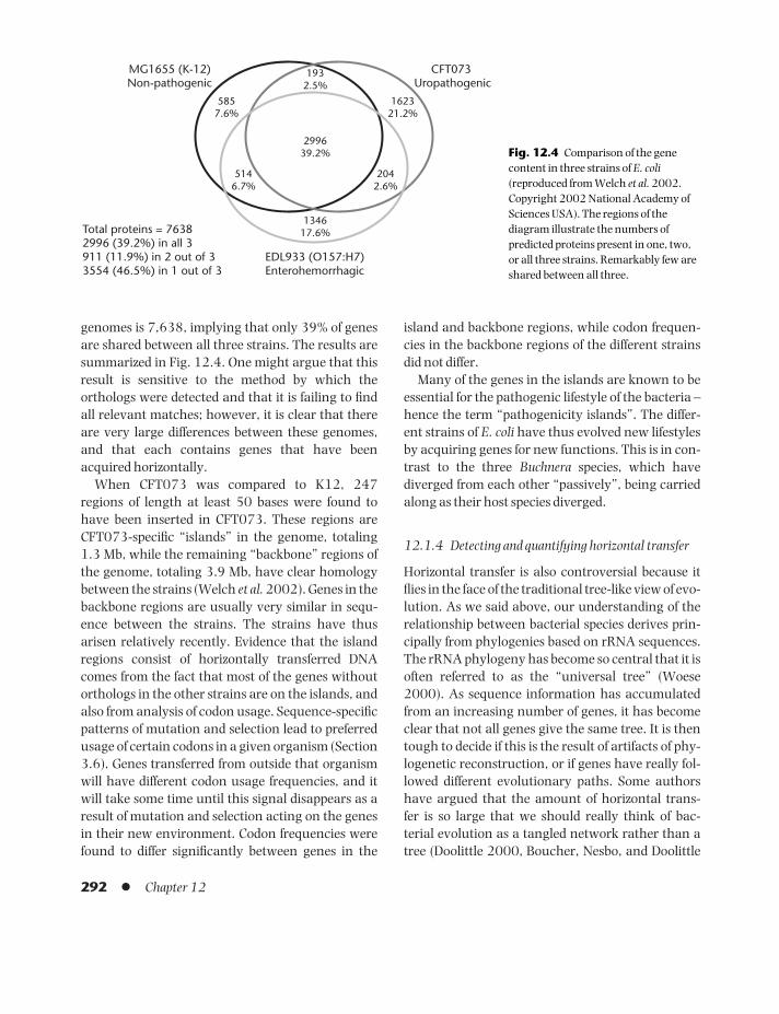
genomes is 7,638, implying that only 39% of genesare shared between all three strains. The results aresummarized in Fig. 12.4. One might argue that thisresult is sensitive to the method by which theorthologs were detected and that it is failing to findall relevant matches; however, it is clear that thereare very large differences between these genomes,and that each contains genes that have beenacquired horizontally.

When CFT073 was compared to K12, 247regions of length at least 50 bases were found tohave been inserted in CFT073. These regions areCFT073-specific “islands” in the genome, totaling1.3 Mb, while the remaining “backbone” regions ofthe genome, totaling 3.9 Mb, have clear homologybetween the strains (Welch et al. 2002). Genes in thebackbone regions are usually very similar in sequ-ence between the strains. The strains have thusarisen relatively recently. Evidence that the islandregions consist of horizontally transferred DNAcomes from the fact that most of the genes withoutorthologs in the other strains are on the islands, andalso from analysis of codon usage. Sequence-specificpatterns of mutation and selection lead to preferredusage of certain codons in a given organism (Section3.6). Genes transferred from outside that organismwill have different codon usage frequencies, and itwill take some time until this signal disappears as aresult of mutation and selection acting on the genesin their new environment. Codon frequencies werefound to differ significantly between genes in the

island and backbone regions, while codon frequen-cies in the backbone regions of the different strainsdid not differ.

Many of the genes in the islands are known to beessential for the pathogenic lifestyle of the bacteria –hence the term “pathogenicity islands”. The differ-ent strains of E. coli have thus evolved new lifestylesby acquiring genes for new functions. This is in con-trast to the three Buchnera species, which havediverged from each other “passively”, being carriedalong as their host species diverged.

12.1.4 Detecting and quantifying horizontal transfer

Horizontal transfer is also controversial because itflies in the face of the traditional tree-like view of evo-lution. As we said above, our understanding of therelationship between bacterial species derives prin-cipally from phylogenies based on rRNA sequences.The rRNA phylogeny has become so central that it isoften referred to as the “universal tree” (Woese2000). As sequence information has accumulatedfrom an increasing number of genes, it has becomeclear that not all genes give the same tree. It is thentough to decide if this is the result of artifacts of phy-logenetic reconstruction, or if genes have really fol-lowed different evolutionary paths. Some authorshave argued that the amount of horizontal trans-fer is so large that we should really think of bac-terial evolution as a tangled network rather than atree (Doolittle 2000, Boucher, Nesbo, and Doolittle

292 l Chapter 12

MG1655 (K-12)Non-pathogenic

CFT073 Uropathogenic

EDL933 (O157:H7)Enterohemorrhagic

Total proteins = 76382996 (39.2%) in all 3911 (11.9%) in 2 out of 33554 (46.5%) in 1 out of 3

1932.5%

134617.6%

5857.6%

162321.2%

5146.7%

2042.6%

299639.2% Fig. 12.4 Comparison of the gene

content in three strains of E. coli(reproduced from Welch et al. 2002.Copyright 2002 National Academy ofSciences USA). The regions of thediagram illustrate the numbers ofpredicted proteins present in one, two,or all three strains. Remarkably few areshared between all three.

BAMC12 09/03/2009 16:36 Page 292

2001). Others argue that it still makes sense to lookfor a core set of genes that are passed down verticallyas a coherent group. Some of the most fundamentalgenes possessed by all domains of life are those con-nected with genome replication and expression, andthese usually give trees consistent with the rRNAtree. Woese (2000) argues that this core set of genesis giving us a valid picture of the organismal genea-logy and defends the idea of a universal tree.

One family of genes for which there is agreementthat horizontal transfer is common is the aminoacyl-tRNA synthetases (aaRSs), which are responsible forcharging tRNAs with their appropriate amino acid.Most organisms have a set of 20 of these genes.Because of their essential role in the translation pro-cess, they occur in all three domains of life, and havebeen widely studied. When phylogenetic trees foraaRS genes are constructed, numerous anomaliesare found, many of which can be explained by hori-zontal gene transfer (Doolittle and Handy 1998,Koonin, Makarova, and Aravind 2001). One inter-esting case is that of GluRS in E. coli. Most eukary-otes have a GluRS and a GlnRS that are related insequence and probably arose via a gene duplicationevent. On the other hand, most bacteria have only aGluRS that is responsible for correctly chargingtRNAGlu and for mischarging tRNAGln with Glu.Correctly charged Gln-tRNAGln is then made fromthe mischarged Glu-tRNAGln by a transamidationreaction that takes place on the tRNA. It is thereforeunusual to find that E. coli and some other pro-teobacteria do possess a GlnRS gene, and do not usethe transamidation route. This indicates horizontaltransfer of a eukaryotic gene into this group of bac-teria. Many other cases of apparent horizontal trans-fer are known in the aaRSs, making them unusual in this respect.

For a horizontally transferred gene to be de-tectable, it needs to survive as a functioning gene inits new host genome. The new gene might replacean existing ortholog that is subsequently deleted, orit might have a useful function not possessed by anyof the host genes. If the horizontally transferred genewere a non-functional pseudogene in its new envir-onment, then it would rapidly accumulate muta-tions, and sequence analysis techniques would be

unlikely to spot it. So, if a family of genes, like aaRSs,is frequently horizontally transferred, this suggeststhat the corresponding proteins can function moreeffectively in a foreign cell than would the products ofmost foreign genes, rather than that the DNA of thesegenes is more likely to be transferred than others. TheaaRSs have to interact with tRNAs, which are veryconservative in their structure; other proteins mightbe involved in large-scale complexes with other fast-evolving proteins, so a horizontally transferredsequence might be unable to function effectively andto replace an existing gene. A contrast is sometimesdrawn between aaRSs and ribosomal proteins. Thelatter must interact with many other proteins andRNAs inside the ribosome, so there is large scope forcoevolution of these genes. Ribosomal proteins haverarely been found to be horizontally transferred.

As a final note of caution, we should rememberthat even rRNA genes, beloved of tree-builders, haveoccasionally been transferred horizontally. Yap,Zhang, and Wang (1999) found that, in the bac-terium Thermomonospora chromogena, there are sixcopies of the ribosomal RNA operon, containingboth SSU and LSU rRNA genes. One of these copies issubstantially different from the other five, but bearsa close relationship to the sequence in the relatedspecies, T. bispora, indicating a likely horizontaltransfer from this species.

Given that horizontal transfer between bacteriaoccurs to some degree, an important aim is to locateparticular cases and to give a quantitative estimateof the frequency of occurrence. One way to do this isto look for regions of a genome that appear to havedifferent properties from the surrounding regions:the codon-usage patterns in islands of the E. coliCFT073 strain discussed above is an example of this.The frequencies of bases in different genomes differsubstantially, so if a foreign piece of DNA is insertedinto a genome, it will often stand out by this alone. Intheir study of the E. coli genome, Lawrence andOchman (1998) measured the GC frequency at thefirst and third positions in each gene. The secondposition was excluded, because it is most con-strained by the genetic code and therefore least vari-able. They defined genes as atypical if the GCfrequency was more than two standard deviations

Genome evolution l 293

BAMC12 09/03/2009 16:36 Page 293

away from the mean for all genes. They then lookedfor genes that appeared to have biased codon usagewith respect to typical E. coli genes. They also tookaccount of the possibility of horizontal transfer ofoperons. If several genes are translationally coupled,but not all of them appear unusual by the statisticsabove, then it is nevertheless likely that the geneswere transferred together as an operon. One factorthat can influence the base composition of genes isthe amino acid composition of the correspondingprotein. For example, Lawrence and Ochman foundsome proteins with large numbers of lysine residues.As the corresponding codons are AAA and AAG, ahigh AT content is apparent in these genes, whichdoes not indicate horizontal transfer.

Combining all these factors, it was estimated that755 of 4,288 ORFs in E. coli had been horizontallytransferred, which is a huge 17.6%. What happensto these genes when they arrive in a new genome?First, they are subject to the mutational biases in thehost organism. This means that any usual base fre-quencies and codon-usage patterns will graduallydecay away until the gene looks just like its sur-roundings. Lawrence and Ochman (1998) had estimates of mutation rates and hence were able toobtain estimates of how long the horizontally trans-ferred genes had been present, by looking at theirbase frequencies. They estimated a mean age of 14.4million years, which translates into an estimatedrate of 16 kb of DNA transferred per million years. Inthe 100 million years since the divergence of E. coliand Salmonella, this means a total of 1.6 Mb has beenadded to the E. coli genome – this should be com-pared to the total genome length of 4.6 Mb. Thelarge rate of gain by horizontal transfer must be bal-anced by a significant amount of random deletion,thus creating a turnover in gene content.

These numbers should be taken with a pinch ofsalt. There is a degree of uncertainty in assigningwhich genes are horizontally transferred, and thereis a large amount of educated guesswork in cal-culating the rates. Nevertheless, the bottom line isthat horizontal transfer seems to be much moreimportant than anyone expected before completegenomes were available. A more recent estimate(Ochman, Lawrence, and Groisman 2000) gives a

horizontal transfer figure of 12.8% of the E. coligenome, which is larger than for all but one of thespecies considered. The figures vary considerablybetween species: e.g., 11.6% of foreign DNA wasfound in Mycoplasma pneumoniae, but none at all inMycoplasma genitalium.

12.1.5 Clusters of orthologous groups (COGs)

When comparing the sets of genes in differentgenomes, a first question is which genes are ortho-logous. Orthologs are genes in different species thatdiverged from a common ancestral sequence as aresult of speciation of the organisms. If differentspecies had exactly the same genes, then it would bepossible to take each gene in one species and find anortholog for it in every other species. However, thereare many genes that are present in some, but not all,of the complete genomes we have available, eitherbecause they have arisen for the first time in certainspecies, or because they have been deleted fromgenomes that originally possessed them. Anothercomplication is gene duplication. Related genes inone genome that have arisen from a common ances-tral sequence by gene duplication are called par-alogs. Many genes in eukaryotes consist of familiesof paralogs. Sometimes, one gene in a bacterialgenome is orthologous to a family of genes in aeukaryotic genome. Duplications can also occurindependently in different lineages, leading to situ-ations where different species each possess familiesof paralogs, but there is no correspondence betweenindividual pairs of genes in the different organisms.In other words, relationships between genes may beone-to-one, one-to-many, or many-to-many. Anexample of complex gene duplications was given forhexokinase genes in Fig. 6.5. Here, there are fourpairs of orthologs between human and rat, whichcan be identified because the gene duplicationsoccurred before the divergence of the human and ratspecies. However, if we compare human with yeast,we can only say that there is a family of paralogs inhumans and a family of paralogs in yeast, but thereis no one-to-one relationship between individualgenes. In this case, we might nevertheless say thatthe two families of genes are orthologous, because

294 l Chapter 12

BAMC12 09/03/2009 16:36 Page 294

the genes that gave rise to the families diverged as aresult of speciation at some point long ago.

The COG (Clusters of Orthologous Groups) data-base was set up to identify related groups of genes incomplete genomes (Tatusov, Koonin, and Lipman1997, Tatusov et al. 2001). Each COG is a set ofgenes composed of individual orthologous genes, or of orthologous groups of paralogs from three ormore species. For each gene in each of the completegenomes analyzed, BLAST was used to find the besthitting gene in each of the other genomes. The clus-tering procedure began by looking for triangularrelationships of genes in three species, such thateach is the best hit of the other two. Whenever twotriangles of genes shared a side, these sets of geneswere combined into one cluster. Although this clustering scheme is relatively simple and easy toimplement automatically, it avoids some of the dan-gers that might arise in some other automatedschemes. For example, best hits according to BLAST(and other search algorithms) are not necessarilythe most closely related when more careful phylogen-etic analysis is carried out. In the COG system, eachmember of a cluster is a best hit of at least two othermembers of the group, which prevents connectingtwo clusters that are only related by spurious singlelinks. Also, the COG system avoids defining a sim-ilarity threshold. It is easy to envisage a system inwhich all sequences are clustered if their similarityscore is above some threshold; but such clusterswould be very sensitive to the threshold chosen. Assome orthologous groups are much more divergentthan others, it would be difficult to choose a thresh-old appropriate to all genes.

The COG database began with seven genomes andfound 720 clusters. The current version has ex-panded to 43 genomes, including Saccharomycescerevisiae as the only eukaryote, and a range of bac-teria and archaea. There are now 3,307 clusters. Ofthe 104,000 genes in the full set of genomes, 74,000of them (71%) have been clustered into COGs. Thepercentage of genes that are clustered tends to belarger for the smaller bacterial genomes: e.g., inBuchnera, 568 out of 575 genes are clustered (99%).As we saw above, Buchnera has retained a relativelysmall fraction of the genes it once had, and those

that are retained appear to be essential genes forwhich it is possible to find orthologs in many otherspecies. On the other hand, in E. coli K12, which hasa much larger genome, 3,414 genes of 4,275 (80%)were clustered. For the considerably larger S. cere-visiae genome, only 2,290 genes of 5,955 (38%)could be placed in COGs. This indicates that a sub-stantial number of genes in eukaryotes do not haveorthologs in prokaryotes. As more complete eukary-otic genomes become available, it will presumablybe possible to cluster many of these genes into COGscontaining only eukaryotic species.

If we consider only the average figure of 71%, thisstill means that there are substantial numbers ofgenes for which no reliable orthologs can be found.How do we interpret this? Some of these genes couldreally be “unique” to a given species or closelyrelated group of species. As more species are added,the chances of finding related species that sharegenes will become larger, hence the number of COGsshould increase and the fraction of genes assigned to them should increase. This has indeed been hap-pening, as can be seen by comparing the figuresabove, from the Web site in December 2003 (http://www.ncbi.nlm.nih.gov/COG/), with thosepublished two years ago (Tatusov et al. 2001).Another interpretation is that our methods fordetecting orthologous sequences are simply notgood enough to detect distant matches (this must beat least partly true, but it is difficult to know howmany matches are being missed). A third possibilityis that some of the ORFs annotated as genes in thepublished genomes are not real genes. By studyingCOGs, Tatusov et al. (2001) gave evidence thatmany of the ORFs originally predicted in Aeropyrumpernix (an archaeon not closely related to previouslysequenced species) were not real genes. COG ana-lysis can also potentially help in genome annotationby detecting missing genes. If a gene is absent in aspecies but present in several related ones, thismight suggest that it has been overlooked, and thata more careful search of the genome is warranted.Another potential use for COGs is that when a genehas been reliably assigned to a cluster, one can inferits function from that of others in the cluster.However, there are still many clusters for which

Genome evolution l 295

BAMC12 09/03/2009 16:36 Page 295

the function is unknown, or at best, only partiallyunderstood.

There are several take-home messages here.Complete genomes are an important resource, butare just a beginning for future studies. Our currentknowledge is insufficient to say with certainty whereall the genes are in a genome. Knowing the completeset of genes does not tell us their functions. Bioin-formatics methods are important for genome annota-tion, and methods that can compare new genomeswith many previously sequenced genomes can leadto a substantial improvement in the reliability ofannotation.

12.1.6 Phylogenies based on shared gene content

Sometimes, phylogenies based on different genes arenot consistent with one another. This may resultfrom inaccuracies or lack of resolution of the meth-ods, or from horizontal gene transfer. Either way, itis interesting to try to build phylogenies based on thedegree of similarity of the gene content of genomesrather than on the similarity of individual genesequences. Arguably, this gives a better picture ofevolution of the whole organism than could beobtained from any single gene.

The first step in this process is to measure thenumber of shared genes between genomes. Snel,Bork, and Huynen (1999) used the Smith–Waterman algorithm to compare all the genes in aset of complete genomes. Genes from two differentgenomes were defined to be orthologs if they wereeach the other’s best hit in the other genome, and if the E value for the alignment was less than 0.01.The more closely related the two genomes, the largerthe number of shared genes we would expect to find.However, genomes differ considerably in the num-ber of genes they possess. Larger genomes are likelyto share larger numbers of genes than smallergenomes. Also, genome size can vary considerablyin closely related organisms, particularly in parasiticand endosymbiotic bacteria, which can lose largenumbers of genes very quickly. To account forgenome size bias, the number of shared genes wasdivided by the number of genes in the smaller of thetwo genomes. This gives a measure of similarity, S,

that varies between 0 (for no shared genes) and 1(where the genes on the smaller genome are a subsetof the genes on the larger). If there were a continualprocess of genome evolution via gain and loss ofgenes, we would expect the similarity between twogenomes to decay roughly exponentially with timesince they diverged. We can therefore define a meas-ure of distance between genomes as d = −ln S. In this way, a matrix of distances between a set of gen-omes can be calculated, and this distance matrix canbe used as input to distance-matrix phylogenetic programs, such as neighbor-joining and Fitch–Margoliash methods (Sections 8.3 and 8.5).

Initial attempts at doing this (Snel, Bork, andHuynen 1999, Fitz-Gibbon and House 1999) usedrelatively small numbers of genomes. Now that sub-stantial numbers of genomes are available, theresults become quite interesting, and Korbel et al.(2002) have set up a Web-based resource, calledSHOT, for doing whole-genome phylogenies of thistype. An example of the output of SHOT is shown inFig. 12.5. Many aspects of this phylogeny confirmwhat was previously deduced from rRNA sequencephylogenies. The division into the 3 domains,archaea, bacteria, and eukaryotes, is clearly shownin the figure. The eukaryotes are divided into ani-mals, fungi, and plants (animals and fungi being theclosest two of the three groups). This point has alsobeen shown using rRNA phylogeny (van de Peer etal. 2000). Unfortunately, there is, as yet, no com-plete genome information on the diverse array ofprotists and other early-branching eukaryotes.Several of the major groups of bacteria known fromrRNA phylogenies are also found in the whole-genome phylogeny. But there are also aspects of thetree that are not well resolved (e.g., branchingwithin the bacteria is rather star-like), or thatconflict with sequence-based phylogenies (e.g., D.melanogaster appears closer to human than to C. elegans, but sequence-based phylogenies place D.melanogaster and C. elegans in the Ecdysozoa groupwithin the Protostomes, with humans as Deutero-stomes (Section 11.3.2)).

It might be hoped that whole-genome phylo-genies would be free of some of the sensitivity ofsequence-based phylogenies to the gene used, the

296 l Chapter 12

BAMC12 09/03/2009 16:36 Page 296

alignment, the choice of species included, and themethod of tree construction. Nevertheless, there aremany factors that enter into whole-genome phylo-genies too. There are several ways to calculate sim-ilarity between genomes. By default, Korbel et al.(2002) now use a weighted average of genome sizesto normalize the number of shared genes, ratherthan dividing by the smaller of the two genomes.The number of shared genes between two genomesdepends on the definition of orthologs and themethod used to detect them. The number of genes on

each genome is also open to question. One mightwish to exclude genes that have no ortholog in anyof the other species. The way distance is calculatedfrom similarity is rather crude, and is not based on awell-defined model of genome evolution. Once wehave a distance matrix, there are many ways to cal-culate a phylogeny from it. Unfortunately, all thesedetails affect the resulting tree to some extent. Weare still in the early days of whole-genome phylogen-etics, and although methods like this are unlikely to solve all the problems, they promise to give

Genome evolution l 297

N. meningitidis A

X. fastidiosa

H. influenzae

P. multocida

T. maritimaB. subtilis

B. halodurans

S. aureus Mu50

L. lactis

S. pyogenes

M. pneumoniae

M. g

enita

lium

U. u

real

yticu

mM

. pul

mon

is

Buchnera

E. coli K12V. cholerae

P. aeruginosaR. prow

azekiiC. crescentus

M. loti

C. m

uridarumC

. pneumoniae C

WL029

H. p

ylor

i 266

95C

. jej

uni

A. a

eolic

usM

. tub

ercu

losi

s

M. l

epra

eD.

radi

odur

ans S. p

ombe

C. a

lbic

ans

S. ce

revis

ae

D. m

elano

gaste

r

H. sapiens

C. elegans

A. thaliana

S. solfataricus

A. pernixT. acidophilumP. abyssi

P. horikoshii

P. fu

riosu

s

A. fu

lgid

us

M. j

anna

schi

i

M. t

herm

oaut

otro

phic

um

Hal

obac

teriu

m

Syne

choc

ystis

B. b

urgd

orfe

ri

T. p

allid

um

Firmicutes

Spirochaetes

Archaea

Plants

Animals

Fungiε Proteobacteria

α Proteobacteria

β + γ Proteobacteria

Fig. 12.5 Phylogeny based on shared gene content of completely sequenced genomes, calculated using the default options of theSHOT program (Korbel et al. 2002).

BAMC12 09/03/2009 16:36 Page 297

increasingly useful information as the number ofcomplete genomes continues to rise.

An interesting study by Snel, Bork, and Huynen(2002) compares gene content among Proteobac-teria and Archaea. Rather than use gene content todeduce the phylogeny, it is assumed that the tree isalready known, and phylogenetic methods are usedto study the mechanisms by which gene contentevolves on this tree. They allow for change in genecontent via gene loss, gene duplication, horizontalgene transfer, and de novo origin of genes. A cost isassigned for changes of each type. The gene contentis known for each species on the tips of the tree. Thegene content of each of the ancestral nodes of thetree is estimated by a type of maximum parsimonyprogram that minimizes the total cost of changes in gene content across the tree. The method can beused to predict the gene content of ancestral gen-omes, and also to give sensible bounds to costs associated with each type of change.

The main factor influencing the results of thisstudy is the relative cost assigned to horizontaltransfer and gene deletion. Whenever a gene is pre-sent in some species but not others, it is possible toexplain this entirely in terms of gene deletions orentirely in terms of horizontal transfer, as shown inthe example of Fig. 12.6. If the cost of horizontaltransfer is very high, the maximum parsimony solu-

tion will use only deletions. As a result, the programwill predict extremely large ancestral genomes con-taining every gene that is present in at least one ofthe species. If the cost of horizontal transfer is low,the solution will not use deletions. Genes will ori-ginate internally within the tree and will be hori-zontally transferred many times. Hence, ancestralgenomes will be predicted to be very small. Snel,Bork, and Huynen (2002) concluded that verticaldescent of genes was the leading factor in genomeevolution (i.e., most genes were transmitted vertic-ally from the preceding node on the tree most of thetime), followed by gene loss and gene genesis.Horizontal transfer was important in explaining thepatterns of presence and absence of genes, but wasless frequent than gene loss and genesis on the basisof the number of events that occurred in the mostparsimonious solution.

12.2 ORGANELLAR GENOMES

12.2.1 Origin of mitochondria and chloroplasts

Both mitochondria and chloroplasts are organellesin eukaryotic cells that are contained in their ownmembranes and that possess their own genomes.The idea that these organelles are descended fromendosymbiotic bacteria has been around for a longtime (Margulis 1981). We have already seen exam-ples of bacteria that live obligately inside larger cells,either as parasites or as symbionts. It seems a rela-tively small step from such bacteria to organellesthat are an integral part of the cell. We now havesolid evidence, from analysis of gene sequences oforganellar genomes, that both mitochondria andchloroplasts arose by endosymbiosis. This has beenshown by many researchers and has been reviewedby Gray and Doolittle (1982) and Gray (1992).

One study that shows this clearly is that ofCedergren et al. (1988). These authors aligned bothSSU and LSU rRNA from representative species ofarchaea, bacteria, eukaryotes, mitochondria, andchloroplasts. An alignment over such a wide rangeis difficult, because of the large variability in lengthbetween the sequences from the different domains.Nevertheless, the secondary structure of these

298 l Chapter 12

AAbsent

BPresent

CPresent

DAbsent

Possibility of twoindependent losses of

the same gene

Possibility of horizontal transfer

Fig. 12.6 The pattern of presence and absence of a gene inthe four genomes shown here can be explained either byhorizontal transfer from B to C, or vice versa, or by twoindependent losses of the gene from species A and D.

BAMC12 09/03/2009 16:36 Page 298

molecules is known and there are some regions thatare very well conserved across all the domains.Cedergren et al. (1988) chose sequence regions fromthe most conserved parts of the secondary struc-ture for their phylogenetic analysis. They found thatthe division of life into the three domains – archaea,bacteria, and eukaryotes – was strongly supported,and that the sequences of mitochondria and chloro-plasts branched within the eubacterial domain. The chloroplast sequences were closely related tocyanobacteria, a group of normally free-living pho-tosynthetic bacteria. This means that photosyn-thesis in eukaryotes (i.e., plants and algae) wasinvented in prokaryotes and acquired by endosym-biosis. The mitochondrial sequences were similar tothose of the α-Proteobacteria, a group that includesintracellular bacteria, such as Rickettsia. The chiefrole of present-day mitochondria is to carry out aer-obic respiration. This means that aerobic respirationwas also invented by prokaryotes and acquired byeukaryotes by endosymbiosis.

Several of the genes involved in the electron trans-port system of the respiratory process are coded onmitochondrial genomes. Two of the most conservedof these are cytochrome c oxidase subunit 1 andcytochrome b. Sicheritz-Ponten, Kurland, andAndersson (1998) compared the sequences of thesetwo genes from mitochondrial and bacterialgenomes. They found that the mitochondrial geneswere related to Rickettsia genes, and they estimatedthat mitochondria and Rickettsia diverged from oneanother 1,500–2,000 million years ago. This is consistent with estimates of the time of origin ofeukaryotic cells from other sources. Another groupof sequences that provide evidence on the origin of organelles are the Hsp60 heat-shock proteins(known as GroEL in bacteria). These are chaper-onins that assist unfolded or misfolded proteins infinding their correct structure. Phylogenetic analysisof these sequences also confirms the relationshipsbetween mitochondria and Rickettsia, and betweenchloroplasts and cyanobacteria (Viale and Arakaki1994). Although the heat-shock proteins are foundin the mitochondria, the genes for these proteins areactually in the eukaryotic nucleus. The interpreta-tion is that the Hsp60 genes entered eukaryotes in

the bacterium that became the mitochondrion, andthat the gene was later transferred from the mito-chondrial genome to the nuclear genome. Manyother genes from organelle genomes have also beentransferred to the nucleus, as we shall see below.

Most mitochondrial genomes are very muchsmaller than bacterial genomes. For example, thehuman mitochondrial genome, which is typical ofanimal mitochondrial genomes, is only 16 kb inlength and possesses 37 genes: 13 protein-codinggenes associated with the electron transport chain,two rRNAs, and 22 tRNAs. The gap between mito-chondria and bacteria has been reduced recently bythe sequencing of several protist mitochondrialgenomes (Gray et al. 1998). The most bacteria-likeof the available mitochondrial genomes is that ofReclinomonas americana (Lang et al. 1997). This is asingle-celled freshwater protist that belongs to agroup known as the jakobids. The genome is oflength 69 kb and contains 97 genes. The proteinspresent include 24 from the electron transportchain, 28 ribosomal proteins (i.e., components ofthe mitochondrial ribosome), four that form an RNApolymerase, six others of various functions, and fiveof unknown function. There are three rRNA genes,as a gene for 5S rRNA is present in addition to theusual SSU and LSU rRNAs. There is also a gene forribonuclease P RNA, not usually found in mitochon-drial genomes, and there is an expanded set of 26tRNAs.

In addition to its having a larger repertoire ofgenes, there are other reasons for concluding thatthe R. americana mitochondrion more closely re-sembles the ancestral bacterial genome than any of the other known mitochondrial genomes. Thefour-component RNA polymerase encoded by thisgenome is similar to those found in bacteria, and it is substantially different from the nuclear encodedsingle-component polymerase that functions inmost mitochondria. This suggests that the single-component polymerase replaced the bacteria-likepolymerase genes fairly early in mitochondrial evo-lution. For several genes, Lang et al. (1997) alsolocated sequence motifs upstream of the start codonsthat appear to be Shine–Dalgarno regions, and sug-gest that translation is initiated in the same way as

Genome evolution l 299

BAMC12 09/03/2009 16:36 Page 299

in bacteria. There are also several operons (i.e.,groups of consecutive, co-transcribed genes) presentin both the R. americana and bacterial genomes.Andersson et al. (1998) compared the mitochon-drial genome of R. americana with the most mitochondria-like of known bacterial genomes,Rickettsia prowazekii. Figure 12.7 illustrates severalregions of conserved gene order between thesegenomes, which are still present despite over 1,500million years of separate evolution. They also car-ried out phylogenetic analysis with ribosomal pro-

tein genes from both mitochondria and chloroplasts,and confirmed the expected relationships of theorganelle sequences to bacteria.

12.2.2 The evolution of eukaryotic cells

Eukaryotic cells are defined by the presence of anucleus with its own nuclear membrane. Where didthe genes in the nucleus come from? Molecular phylo-genies showing the three domains of life cannot tellus whether eukaryotes are more closely related

300 l Chapter 12

ReclinomonasamericanamtDNA

Rickettsiaprowazekii

Prototheca wickerhamii

Marchantia polymorpha

Reclinomonas americana

Rickettsia prowazekii

Aquifex aeolicus

Borrelia burgdorferi

Helicobacter pylori

Haemophilus influenzae

Escherichia coli

Mycobacterium tuberculosis

Bacillus subtilis

Synechocystis sp.

Porphyra purpurea

Cyanophora paradoxa

100, 100

100, 100

100, 100

100, 100 91, 90

Mitochondria

(b)

(a)

α-Proteobacteria

Cyanobacteria

Chloroplast

97, 91

Nad11, 1, Cox11, 3

L11-L1-L10-RNAPβ-RNAPβ'-S12-S7-EFTu-S10-spc-α

S12-S7-EFG-L11-L1-L10-L12-RNAPβ-RNAPβ'-

EFTu-S10-spc-α

Fig. 12.7 Comparison of a bacteria-like mitochondrial genome fromReclinomonas americana with amitochondria-like bacterial genomefrom Rickettsia prowazekii (reproducedfrom Andersson et al. 1998, withpermission of Nature PublishingGroup). (a) Several regions of conservedgene order are illustrated. S10, spc, andα are each operons composed of severalconsecutive genes. (b) The phylogeny,constructed using ribosomal proteingenes from bacteria, mitochondria, andchloroplasts, demonstrates that themitochondria are related to Rickettsiaand the chloroplasts to cyanobacteria.

BAMC12 09/03/2009 16:36 Page 300

to bacteria or to archaea, because trees like this areunrooted. As we are talking about the whole of life,there is no outgroup species that can be used to pro-vide a root. This problem was overcome by usingpairs of genes that were duplicated prior to the diver-gence of the three domains. Species from eachdomain therefore possess both genes. Phylogeniesconstructed from these gene pairs have two halves,each half providing a root for the other half. Anexample is the two-elongation factor genes, part ofthe translation apparatus. Iwabe et al. (1989) andGogarten et al. (1989) concluded that the root lies onthe branch leading to bacteria, and hence thateukaryotes are more closely related to archaea. Theimplication is therefore that eukaryotes arose froman ancestor that was something like an archaeon.However, some protein phylogenies suggest thateukaryotes are closer to some taxa within the bacteria. Golding and Gupta (1995) argued for achimeric origin of the eukaryotic nucleus, possiblyby fusion of an archaeon and a bacterium. However,if horizontal gene transfer was frequent in the earlystages of cellular evolution, then it may be that a eukaryotic genome acquired genes from many different sources at different times. Philippe andForterre (1999) reanalyzed the data on the rootingof trees using duplicate genes. They found that treesderived from different gene pairs were often incon-sistent, and they also emphasized the problems ofmutational saturation and long-branch attractionthat arise in phylogenies with very divergentsequences. They concluded that the rooting of thetree of life in the eubacterial branch cannot be reliedon. Thus, the origin of the nuclear genome ofeukaryotes is much less clear than the origin of theorganellar genomes.

At what point did the primitive eukaryote acquiremitochondria? Our understanding of this is linked toour interpretation of the phylogeny of the early-branching eukaryotes (we touched on this inSection 11.3.3). Most eukaryotes contain mito-chondria, but there are several groups that do not.In some studies, these amitochondriate groupsappeared at the base of the tree, and were hencereferred to as Archezoa, implying that these groupswere ancient taxa that branched off the main

eukaryotic line prior to the endosymbiosis event. Inother words, it was assumed that the Archezoanever possessed mitochondria. However, severalgroups formerly called Archezoa have been found tobe closely related to crown eukaryote groups inmore recent trees (Embley and Hirt 1998, Roger1999). There have also been cases where genesthought to have originated from mitochondrialgenomes have been found in nuclear genomes ofspecies that do not possess mitochondria. This sug-gests that these groups must have once had mito-chondria and then lost them at a later stage. Thus, itis not clear whether any of the current species lack-ing mitochondria are actually descended entirelyfrom organisms that never had mitochondria.

It is generally assumed that the endosymbiosisevent leading to the origin of chloroplasts happenedafter that leading to mitochondria, as there aremany eukaryotes lacking chloroplasts but very fewlacking mitochondria. There are several types ofchloroplast-containing algae that derived from theinitial incorporation of the cyanobacterium. Some ofthese later evolved into land plants. It is fairly certainthat the chloroplasts in all these organisms derivefrom a single endosymbiosis event (Gray 1992,Douglas 1998). However, there are many otherchloroplast-containing eukaryotes that are thoughtto derive from secondary endosymbiosis events, inwhich an alga arising from the primary event isincorporated inside another eukaryotic cell. Sec-ondary endosymbiosis seems to have occurredmany times (Douglas 1998). Some of these cells stillcontain nucleomorphs (which are the remnants ofthe nucleus of the algal cell incorporated in the sec-ondary event), in addition to a full eukaryoticnucleus deriving from the new host cell.

12.2.3 Transfer of organellar genes to the nucleus

The number of genes in chloroplast and mitochon-drial genomes has reduced tremendously since theirintegration into the eukaryotic cell. We already sawa tendency to reduction of genome size in intracellu-lar bacteria, like Buchnera and Rickettsia, resultingfrom loss of genes that were no longer necessary to the bacteria because the host cell provided

Genome evolution l 301

BAMC12 09/03/2009 16:36 Page 301

substances that would otherwise need to be made by a free-living species. However, organelles havegone a lot further than this. The majority of proteinsnecessary for the function and replication of theorganelles have been lost from the organellargenome and transferred to the nucleus.

In well-studied species like humans and yeast,most nuclear genes for mitochondrial proteins havebeen identified. There is a specialized database of human mitochondrial proteins (http://bioinfo.nist.gov:8080/examples/servlets/index.html) thatgives details of both nuclear and mitochondria-encoded proteins in the mitochondrion. We there-fore know that transfer of genes to the nucleus hasbeen frequent in the past – but is it still going on? Oneway to answer this is to search for sequence similar-ity between mitochondrial and nuclear genomes ofthe same species. Blanchard and Schmidt (1996)developed a computational strategy for doing thisand found a variety of identifiable mitochondrialsequences in humans, yeast, and other species.Many of these inserted sequences are just fragmentsthat do not encode whole genes, and therefore arenot important evolutionarily. However, the longestsection found in the human genome was over 3,000 bp and contained tRNA and rRNA sequences.

The location of mitochondrial DNA fragments inthe nucleus demonstrates that transfer may still bepossible, but it does not demonstrate that the trans-ferred genes can be established as functionalreplacements of the gene in the mitochondrion. Infact, in animal (i.e., metazoan) mitochondria, trans-fer seems to have stopped some time ago. Animalmitochondrial genomes have a very reduced num-bers of genes, but almost exactly the same set ofgenes is found in all animal phyla. Thus, the genecontent of these genomes was established before thedivergence of the animal phyla and has remainedconstant for over 500 million years. In the floweringplants, however, many cases of recent (i.e., in thelast few hundred million years) transfer from bothchloroplast and mitochondrial genomes to thenucleus are known. For example, Adams et al.(2000) showed that there have been 26 independ-ent losses of the ribosomal protein gene rps10 fromthe mitochondrion in a set of 277 plant species.

Similarly, Millen et al. (2001) demonstrated the lossof the translation initiation factor 1 gene infA fromchloroplast genomes of 24 separate lineages in a setof 300 plant species. The number of times thesegenes have been independently established in thenucleus is not known, but is presumed to be large.

The above studies were done using Southern blothybridizations to probe for the presence of a knowngene. When complete organelle genomes areknown, a much more complete analysis is possible.Martin et al. (1998) studied a set of nine completechloroplast genomes, with a cyanobacterial genomeas an outgroup. They identified 205 genes present in at least one of the chloroplasts that must havebeen present in the common ancestral chloroplastgenome. Of these, 46 were still found in all genomes.These gene sequences were used to construct amolecular phylogeny for the species. With this phy-logeny, it was possible to study the process of lossthat had occurred in the remaining 159 genes,using a parsimony principle. It was found that 58genes had been lost once only, but 101 genes hadbeen lost more than once (including a few that hadbeen lost four times independently from the set ofonly nine species). Thus, parallel losses of the samegene occurred very frequently.

Transfer of an organelle gene to the nucleusinvolves several steps. First, a copy of a piece oforganelle DNA has to find its way into the nucleus.The fragment then has to insert itself into thenuclear genome in a position that does not inter-rupt an existing gene. It also has to acquire a pro-moter, so that it gets expressed in the nucleus. Thenit has to find a way of getting its protein product back to the organelle. Proteins destined to be tar-geted to organelles usually have signal peptidesattached to the ends of their sequences. The cell has mechanisms to recognize such labeled proteinsand transport them. One way in which a new organelle-targeted gene might be established is toinsert itself next to a duplicate copy of the promoterand signal peptide region of an existing mitochon-drial gene.

All these steps cannot be as unlikely as they seem,given the fact that transfers do occur frequently. Ifthe process goes to the stage described above, it

302 l Chapter 12

BAMC12 09/03/2009 16:36 Page 302

means that there is now a functioning copy of thegene in both the organelle and the nucleus (notethat the gene in the organelle cannot be deletedunless there is a functioning copy in the nucleus,assuming that it is an essential gene for the function-ing of the organelle). From this point, it is necessaryto think about population genetics. Why should thegene from the organelle be deleted in preference tothe copy in the nucleus? The nuclear genome usu-ally reproduces sexually and undergoes recombina-tion, whereas the organelle multiplies asexually.This means that the organelle genome is subject tothe accumulation of deleterious mutations viaMuller’s ratchet. It might also be argued that thepresence of recombination makes it more likely for afavorable mutation to become fixed in the sequenceof the nuclear copy. Either way, if the nuclear copybecomes fitter than the organelle copy after a certaintime, it is more likely that the organelle copy will beeliminated. Another relevant factor is the differencein rate of mutation in the different genomes. Animalmitochondrial genes accumulate substitutions at afar greater rate than nuclear genes or typical bac-terial genes – see, for example, the rRNA trees ofCedergren et al. (1988), in which the animal mito-chondrial sequences appear on extremely longbranches. However, in plants, mitochondrial substi-tution rates are low in comparison to both nuclearand chloroplast rates (Wolfe, Li, and Sharp 1987). Alarge part of the variation in substitution rates canbe attributed to variation in mutation rates. Themutation rate clearly affects the likelihood of accu-mulation of both favorable and unfavorable muta-tions in the two gene copies. Another factor is thatorganelle genomes from which a gene has beendeleted may also have a selective advantage in speedof replication over longer genomes, and this mighttend to favor the fixation of deletions into the popu-lation. For further discussion of these issues, seeBlanchard and Lynch (2000) and Berg and Kurland(2000).

We might wonder why the organelle retains agenome at all. The purpose of the mitochondrialgenome seems to be to code for the proteins of theelectron transport chain. However, some of thesehave already been transferred to the nucleus, so why

not the rest? The system seems inefficient: if somegenes are maintained in the organelle, then it is alsonecessary to maintain genes involved in the transla-tion of those genes, like the rRNAs and tRNAs and(in some organelles) the ribosomal proteins. It hasbeen suggested that the genes that remain are thosethat could not easily be transported to the organelle,because they are large hydrophobic proteins withseveral membrane-spanning helices. It has alsobeen suggested that these proteins might be harmfulto the cell if expressed in the cytoplasm. However,there is no clear answer to this question yet.

On the theme of the inefficiency of organellargenomes, consider the 35 kb organellar genome ofthe malaria parasite Plasmodium falciparum (Wilsonet al. 1996). This appears to resemble chloroplastgenomes from green algae, although P. falciparum isnot photosynthetic. The genome contains rRNAs,tRNAs, ribosomal protein genes, and RNA poly-merase genes, all of which are necessary purely for the transcription and translation of just threeother genes. Despite the degenerate nature of thisgenome, it has been maintained in the group of apicomplexans, suggesting that it has a key functionfor the organism that is still not understood.

Despite the many losses of genes from organelles,there are relatively few cases of genes found to beinserted into organelle genomes. The probable sim-ple explanation of this is that, for many types oforganelle, it is physically difficult for DNA to get itselfinside the organelle membrane. Plant mitochon-drial genomes appear to be an exception to this.They are much larger than animal mitochondrialgenomes owing to the presence of large amounts ofnon-coding sequence. Due to extensive variability inthe lengths of the non-coding sequences, the num-ber of genes does not correlate with the genome size.In the model flowering plant Arabidopsis thaliana,there are 58 genes in a length of 367 kb; in the liver-wort Marchantia polymorpha, there are 66 genes in 184 kb; and in the green alga Prototheca wicker-hamii, there are 63 genes in 58 kb (Marienfeld,Unseld, and Brennicke 1999). There has thus been a large expansion of genome size in the plant lin-eage. There is evidence for the insertion of nuclearDNA into the A. thaliana mitochondrial genome.

Genome evolution l 303

BAMC12 09/03/2009 16:36 Page 303

However, this does not consist of nuclear genes, butrather of copies of retrotransposons, which aremobile elements able to copy and insert themselves,usually within the nuclear genome itself. The A.thaliana mitochondrial genome does not contain afull set of tRNA genes, which means that sometRNAs must be imported into the organelle. Of thetRNA genes that are found in the mitochondrialgenome, some appear to be of chloroplast ratherthan mitochondrial origin. This is the only knowncase of chloroplast genes being transferred to mito-chondrial genomes.

12.2.4 Gene rearrangement mechanisms

Animal mitochondrial genomes provide good exam-ples for looking at the processes leading to change ingene order. More than 470 of these genomes havebeen completely sequenced, and almost all containthe same set of 37 genes, but these occur in manydifferent orders in different species. The OGRe(Organellar Genome Retrieval) database storesinformation on complete animal mitochondrialgenomes and allows visual comparison of any pair ofgenomes ( Jameson et al. 2003). The examplesshown in Plate 12.2 depict mitochondrial genomeslinearly – it should be remembered that they areactually circular and that the two ends are con-nected. Genes on one strand, transcribed from left toright, are drawn as boxes below the central line, andgenes on the other strand, transcribed from right toleft, are drawn as boxes above the line.

Plate 12.2(a) shows the human mitochondrialgenome. The 13 protein-coding genes are shown ingreen, the two rRNAs in blue, and the 22 tRNAs ingreen. The genome has almost no space between thegenes, with the exception of one large non-codingregion, which is the origin of replication for thegenome. The same gene order occurs in all placentalmammals, and many other vertebrates too. Birds,however, differ from mammals. Plate 12.2(b) com-pares the human and chicken mitochondrialgenomes. Regions of the genomes in which the geneorder is the same in both species are shown in thesame color. Points on the genome where the geneorder changes between the two species are called

breakpoints. There are three breakpoints in thehuman–chicken example. In this case, the yellowblock, containing one protein and two tRNAs, hasswitched positions with the red block, containingone protein and one tRNA.

We can represent this process as

1,2,3,4 → 1,3,2,4

where each number represents a gene or a block ofconsecutive genes. There are several ways in whichthe order of the two blocks can be reversed. One is bya translocation, in which one of the blocks is cut outand reinserted in its new position. A second possibil-ity is an inversion, in which a segment of the genomeis reversed and reconnected in the same position,thus:

1,2,3,4 → 1,−3,−2,4

Here, the minus signs in front of 2 and 3 indicatethat these genes (or gene blocks) are now on theopposite strand and transcribed in the oppositedirection. Note that this is not what happened in thehuman–chicken case, because the red and yellowblocks are on the same strand in both species.Switching two blocks while keeping them on thesame strand can be achieved with three separateinversions, like this:

1,2,3,4 → 1,−2,3,4 → 1,−2,−3,4 → 1,3,2,4

However, this would mean that three inversions hadoccurred in the same place on the genome in a shortspace of time, without leaving any surviving specieshaving the intermediate gene orders. This does notseem like a parsimonious explanation.

There is another, quite likely way in which theinterchange in human and chicken could have oc-curred. This is via duplication followed by deletion.

1,2,3,4 → 1,2,3,2,3,4 → 1,2/ ,3,2,3/ ,4 → 1,3,2,4

In this case, a tandem duplication of the region2,3 has occurred (e.g., because of slippage during

304 l Chapter 12

BAMC12 09/03/2009 16:36 Page 304

DNA replication). There are now redundant copiesof these two genes and we expect one or other copyto disappear rapidly as a result of accumulation ofdeleterious mutations and deletions, and possiblyselection for minimizing the genome length. Afterthe duplicate copies have disappeared, we are leftwith genes 2 and 3 in reverse order. However, if thecentral 3,2 pair had been deleted instead, the originalgene order would have been maintained.

This mechanism seems likely whenever we seeswitching of order within two short neighboringregions. A case where the same mechanism seemsextremely likely (Boore and Brown 1998) is in theregion containing the consecutive tRNAs W,–A,–N,–C,–Y (the letters label tRNA genes according to their associated amino acid). This is shown on the right of the human genome diagram in Plate12.2(a). This order occurs in the platypus, echidna,and in placental mammals, but in all the marsupialssequenced so far, the order is –A,–C,W,–N,–Y. Thiscan be explained by a duplication and deletion offour genes:

W,–A,–N,–C,–Y →W,–A,–N,–C,W,–A,–N,–C,–Y →–A,–C,W,–N,–Y

Note that all the genes remain on the same strand,so it is unlikely that this occurred by inversions.Interestingly, the change is not reversible: if the four genes A,–C,W,–N in the marsupials are duplic-ated, it is not possible to return to the order in theplacentals.

The mobility of tRNA genes within the mitochon-drial genome is illustrated in Plate 12.2(c). Thiscompares two insect genomes (honey bee andlocust). There are some long expanses of unchangedgene order, but there are also areas with complexreshufflings of tRNAs, including long-distancejumps of E and A. Ignoring the tRNAs, the order ofthe proteins and rRNAs is identical.

When genomes from different animal phyla arecompared, complex rearrangement patterns areoften seen. However, if tRNAs are excluded, a simplepattern sometimes emerges for the rearrangementof the proteins and rRNAs. In the comparison of amollusc and an arthropod shown in Plate 12.2(d),

the blue gene block has been translocated and theyellow gene block has been inverted. This can becompared with the much more complex pattern ofmovement when tRNAs are included (see the OGReWeb site, Jameson et al. 2003).

12.2.5 Phylogenies based on gene order

Gene order has the potential to be a strong phylo-genetic marker. There are so many different possibleorders, even for a small genome like the mitochon-drial genome, that when conserved patterns of geneorder are seen, they are unlikely to have arisen twiceindependently. For example, the tRNA rearrange-ment shared by the marsupials would be a strongargument that these species form a related group,had we not already known this from a wealth of otherevidence. In some cases, however, gene order canprovide a strong argument to resolve issues for whichthere is no conclusive evidence from other sources.

One such case is the relationship between the fourmajor groups of arthropods: chelicerates (e.g., spiders,scorpions); myriapods (centipedes and millipedes);crustaceans; and insects. Taxonomists have disagreedabout this for decades, but one hypothesis that hadgenerally been accepted is that myriapods and insectswere sister groups. However, Boore, Lavrov, andBrown (1998) compared the mitochondrial geneorder of these groups and found that insects andcrustaceans shared a genome rearrangement notpresent in myriapods and chelicerates. By consider-ing gene orders from outside the arthropods, theywere able to show that the chelicerates and myriapodshad retained features of gene order present in otherphyla, and hence that the rearrangement in insectsand crustaceans is a shared derived feature thatlinks these as sister groups. Roehrdanz, Degrugillier,and Black (2002) have continued this approach,looking at the relationships between subgroups ofarthropods at a more detailed level. Scouras andSmith (2001) give another good example of howgene order information can be linked to molecularphylogenies for several groups of echinoderms.

In cases such as those above, where clear sharedderived features of gene order are located, this givesimportant phylogenetic information in a qualitative

Genome evolution l 305

BAMC12 09/03/2009 16:36 Page 305

way. However, there have also been attempts todevelop more general computational algorithms todeduce phylogeny from gene order. As with sequence-based methods, the simplest to understand are distance-matrix methods. First, we need to define ameasure of distance between two gene orders. Wecan then determine a matrix of distances for eachpair of genomes in the set considered, and input thismatrix to any of the standard methods, like neighbor-joining and Fitch–Margoliash (see Chapter 8).

The issue, then, is how to measure distances be-tween gene orders. One possibility is simply to countthe number of breakpoints (Blanchette, Kunisawa,and Sankoff 1999). This is an intuitively easy-to-understand measure of how much disruption of thegene order there has been. It is also very simple tocalculate. However, it is not directly related to anyparticular mechanism of genome rearrangement.Other possible types of distance are edit distances(Sankoff et al. 1992), which measure the minimumnumber of editing operations necessary to transformone gene order into another. The simplest of thesewould be the inversion distance, in which the onlyediting operations allowed are inversions of a con-secutive block of genes. Distances can also be cal-culated that allow a combination of translocationsand inversions (Blanchette, Kunisawa, and Sankoff1996).

Although the principle of these edit distances issimple to state, the algorithms for calculating themare complex (see Pevzner 2000, and referencestherein). If the genes in a genome are numberedfrom 1 to N, then a possible gene order can be rep-resented as a permutation of these numbers. Somealgorithms deal with unsigned permutations, i.e.,the strand a gene is on and its direction of transcrip-tion are ignored, and only the position of the genematters. However, it is much more realistic to treatgene orders as signed permutations, as in the exam-ples in Section 12.2.4, in which case a minus signindicates a gene on the opposite strand. It turns outthat there is an exact algorithm for the inversion dis-tance (i.e., sorting signed permutations using onlyinversions) that runs in polynomial time. How-ever, no such algorithm is known for edit distancesthat use translocations as well; hence, combined

inversion–translocation distances have to be cal-culated heuristically by trying many possible path-ways of intermediates between the two genomes.

Somewhat surprisingly, it has been shown that, inproblems with real genomes, the simple breakpointdistance is very close to being linearly propor-tional to both the inversion distance and the com-bined inversion–translocation distance (Blanchette,Kunisawa, and Sankoff 1999, Cosner et al. 2000).This means that if the distance matrices calculatedwith the different measures of distance are put intophylogenetic algorithms, the same shaped tree willemerge. This is an argument for using the simplestmeasure of distance, i.e., the breakpoint distance.

There are also several methods for constructinggene-order trees that can be thought of as maximumparsimony methods. With “normal” parsimony, usingcharacter states coded as 0 or 1 (Section 8.7.1), theparsimony cost for a given tree is the sum of thenumber of character-state changes over the wholetree, and the tree with the minimum cost is selected.To calculate the cost for any given tree, it is necessaryto determine the optimal values of the character stateson each internal node, and then to sum the changesnecessary along each branch of the tree. This is directlyanalogous to the minimal-breakpoint tree method ofBlanchette, Kunisawa, and Sankoff (1999). Here, agene order is assigned to each internal node of a treein such a way that the sum of the breakpoint distancesalong all branches of the tree is minimized. The treeis then selected that minimizes this minimum value.Bourque and Pevzner (2002) have also developed asimilar method, where gene orders on the internalnodes are calculated so as to minimize the sum of theinversion distances along all the branches.

Another parsimony method for gene order(Cosner et al. 2000) creates a set of binary charactersthat represent each gene order and inputs the binarycharacters into a normal parsimony program. Eachcharacter represents the presence or absence of aconsecutive gene pair in the order. Consider the fourgene orders below:(i) 1,2,3,4(ii) 1,−3,−2,4(iii) 1,2,–3,4(iv) 1,3,2,4

306 l Chapter 12

BAMC12 09/03/2009 16:36 Page 306

The character for the pair 2,3 would be assigned to 1in (i) and also in (ii), because these genes are stillconsecutive and run in the same direction relative toone another, whereas it would be assigned to 0 in(iii) and (iv). A parsimony program will be able toreconstruct the most parsimonious assignments ofthe character states on all the internal nodes. Themethod has the drawback that not every possible setof 0s and 1s that might arise on the internal nodesrepresents a valid gene order. This is because thecharacters are not independent. For example, if thepair 2,3 is present, then the pair 2,4 cannot be pre-sent in the same genome. Parsimony programs treateach character as being independent. Despite thisdrawback, Cosner et al. (2000) found this methoduseful. They use it to generate trial trees that theythen screen using other criteria.

Another gene-order phylogeny method worthmentioning is the Bayesian approach of Larget et al.(2002). This is the only method to date that has anexplicit probabilistic model of genome rearrange-ments. The only events permitted are inversions.The number of inversions that occur on a branchhas a Poisson distribution, with a mean proportionalto the branch length. A trial configuration consistsof a tree with specified branch lengths and specifiedpositions of inversions. It is possible to calculate thelikelihood of any given configuration according tothe probabilistic model. A Markov Chain MonteCarlo (MCMC) method is then used to obtain a rep-resentative sample of configurations weighted accord-ing to the model.

There are as yet rather few data sets that can beused with these methods, and it remains to be seenjust how useful the algorithms will be. Sankoff et al.(1992) studied mitochondrial genomes of fungi anda few animals. Chloroplast genomes have been stud-ied for the Campanulaceae family of flowering plants(Cosner et al. 2000) and for the photosynthetic protists (Sankoff et al. 2000). The animal mitochon-drial genomes have been studied several times, butthe results are not as good as might be hoped.Distance-matrix methods using breakpoint distance(Blanchette, Kunisawa, and Sankoff 1999) failed to place the Deuterostomes (i.e., Chordates +Echinoderms) together in a clade, and failed to place

the Molluscs together. These are things thatsequence-based phylogenies would have no prob-lem with. The minimal-breakpoint tree method wasconsiderably better – it did find both of these clades,but placed the Arthropods as sister group to theDeuterostomes, rather than as part of the Ecdysozoa,as expected from sequence-based phylogeny (Section11.3.2). With the method of Bourque and Pevzner(2002), neither the Arthropods nor the Molluscsappeared as monophyletic groups. With the methodof Larget et al. (2002), a wide variety of alternativetree topologies arose in MCMC simulations, and theposterior probabilities did not strongly discriminatebetween alternatives. There was also a tendency for the Molluscs to be polyphyletic and, for some reason, the human tended to cluster with echino-derms rather than the chicken. The phylogeny of the animal phyla is still not well understood, andadditional evidence deriving from gene order wouldbe welcome. However, the results from these studiesof mitochondrial gene order do not seem sufficientlyreliable to draw firm conclusions.

The reason for this may lie in the gene ordersthemselves, rather than with problems in the meth-ods. Several of the animal phyla contain both con-servative and highly derived gene orders. There is atendency for all the methods to group the more con-servative genomes from different phyla together,and to form another separate group of all the highlyderived genomes. This is particularly a problem withthe distance-matrix methods, but it probably alsounderlies the difficulties encountered by the othermethods. Table 12.2 shows breakpoint distancesbetween mitochondrial genomes, calculated bothincluding and excluding the tRNA genes. As we can-not show the whole matrix, we simply give distancesfrom one example species, Limulus polyphemus, thehorseshoe crab. Limulus is thought to be a fairlyprimitive arthropod, and is phylogenetically relatedto the arachnids. Examination of the gene order suggests that it has retained the order possessed bythe ancestral arthropod, or is at least very close.Measuring distances from Limulus to the otherarthropods therefore tells us how much changethere has been within the arthropod phylum, whiledistances from Limulus to non-arthropod species are

Genome evolution l 307

BAMC12 09/03/2009 16:36 Page 307

a good indication of how much change there hasbeen between phyla.

The species in each of the boxes corresponding tothe taxa in Table 12.2 should be equidistant fromLimulus in terms of the time since the commonancestor. However, the breakpoint distances differtremendously for the species in each box. For thetwo closely related tick species, the genome of I. per-sulcatus has remained unchanged, while that of R.sanguineus is highly derived. In the other arthropods(i.e., non-arachnids), there are many examples ofinsects and crustaceans, like D. melanogaster and A.franciscana, where there has been very little change,but there are also examples of unusual species, likeT. imaginis and P. longicarpus, whose genomes appearto have been completely shredded and reassembled.In these latter two cases, we know that a lot ofgenome rearrangement has occurred in an isolatedlineage of organisms in a short time. We have no

idea why these particular genomes should havebeen so unstable.

When comparing genomes between phyla, thedistances that exclude the tRNAs are probably moreinformative – some of the distances with tRNAs areas large as 37, meaning that there is complete ran-domization, with a breakpoint after every gene.Each phylum is seen to contain conservative geneorders (e.g., K. tunicata, T. retusa, H. sapiens) anddivergent ones (e.g., C. gigas, T. transversa, P. lividus).All nematode species sequenced to date seem fairlydivergent. Thus, there is little support for the idea ofgrouping arthropods and nematodes together asEcdysozoa. However, the nematodes are not similarto any other group either, so this just represents lackof evidence for Ecdysozoa, rather than positive evid-ence for an alternative. Another interesting point is that the Deuterostomes are rather less divergentthan most phyla, and hence appear closer to the

308 l Chapter 12

Table 12.2 Breakpoint distances between mitochondrial genomes obtained from OGRe (Jameson et al. 2003). Distances aremeasured from the horseshoe crab, Limulus polyphemus, to the species listed.

Taxon Species Common name Distance Distanceexc. tRNAs inc. tRNAs

Arachnids Ixodes persulcatus Tick 0 0Rhipicephalus sanguineus Tick 3 7

Other Arthropods Drosophila melanogaster Fly 0 3Locusta migratoria Locust 0 6Artemia franciscana Shrimp 0 7Pagurus longicarpus Hermit crab 5 18Thrips imaginis Thrips 11 31

Nematodes Trichinella spiralis Worm 8 21Caenorhabditis elegans Worm 14 37

Molluscs Katharina tunicata Chiton 5 20Loligo bleekeri Squid 4 27Cepaea nemoralis Snail 13 35Crassostrea gigas Oyster 14 37

Brachiopods Terebratulina retusa Brachiopod 5 26Terebratalia transversa Brachiopod 13 37

Deuterostomes Homo sapiens Human 5 20Paracentrotus lividus Sea urchin 10 32

BAMC12 09/03/2009 16:36 Page 308

arthropods than many of the other Protostomes. Onreflection, therefore, it is not too surprising thatthese methods had problems with the animal mito-chondrial genomes. We may remain optimistic that

gene-order phylogeny methods may prove to bemore useful in future, as new, larger, and hopefullyless badly behaved data sets emerge. Such methodsare also applicable to bacterial genomes.

Genome evolution l 309

SUMMARYThere are now many complete bacterial genomes avail-able, and comparisons can be made across a large num-ber of species. Bacterial genomes range in size fromaround half a million to over seven million bases. Thenumber of genes per genome varies almost in pro-portion to the length, with an average of just over 1000bases between gene start points. There is relatively littlenon-coding DNA between genes in bacteria. This sug-gests that selection for efficiency of genome replicationis strong enough to prevent the widespread accumula-tion of repetitive sequences and transposable elements,in contrast to the situation in many eukaryotes.

Genome size and content can vary quite rapidlybetween related bacterial species. The smallest genomesare in bacteria that are parasites or symbionts insideother cells. These species manage with a greatly reducedset of genes, presumably because they can absorb usefulchemicals from their host cell that would have to be syn-thesized by their free-living relatives. There are severalindependent groups of parasitic bacteria where dram-atic reduction of genome size has occurred in this way.This suggests that there is a tendency for genes that areno longer necessary for an organism to be deleted fromgenomes in a relatively short period.

In cases where more than one strain of a bacterialspecies has been completely sequenced, there can be asurprising degree of variability in gene content betweenthe genomes. A notable case is E. coli, where the available pathogenic and non-pathogenic strains con-tain substantially different sets of genes. In pathogenicstrains, it is often possible to identify specific regions ofthe genome, called pathogenicity islands, that containgenes responsible for their pathogenic lifestyle, and thatappear to have been inserted into the genome from else-where. Horizontal transfer of genes between unrelatedbacterial species appears to occur quite frequently on anevolutionary time scale. It is possible to identify recentinsertions by looking for regions with unusual base fre-quencies and codon usage that does not follow the usualcodon bias of the organism. Horizontal transfer alsoleads to inconsistencies in phylogenetic trees derivedfrom different genes.

There is good evidence that both mitochondria andchloroplasts are descended from bacteria that weretaken up by ancient eukaryotic cells, became endosym-bionts, and eventually became integral parts of theeukaryote. Analysis of genes from organelle genomesshows that mitochondria are related to a-Proteobacteria,such as the present-day Rickettsia, and chloroplasts arerelated to cyanobacteria. Organelle genomes encodegreatly reduced numbers of genes by comparison witheven the smallest bacterial genomes. Many of the geneslost from the organelles have been transferred to thenuclear genome. Proteins required in the organelles thatare the product of nuclear genes have acquired a signalpeptide, which tells the cell to transport these proteinsto the organelle. In animal mitochondrial genomes, theprocess of transfer of genes to the nucleus appears tohave come to an end, leaving a small set of essentialgenes on the mitochondrial genome that has been stablethroughout the evolution of the metazoa. In chloroplastsand plant mitochondria, cases of evolutionarily recentgene transfers to the nucleus are known.

There have been attempts to use both gene contentand gene order of complete genomes to deduce evolu-tionary relationships between them. It is possible thatphylogenies based on whole-genome characteristicsmay give a more reliable picture of the evolution of thewhole organism than could be obtained from sequence-based phylogeny with any single gene. With bacteria,measures of distance between genomes have beendefined, based on shared gene content, and these havebeen used in distance-matrix phylogenetic methods.The results have considerable overlap with the treesderived from rRNA sequences. In the case of gene order,distance between two genomes can be defined either interms of the number of breakpoints, or in terms of thenumber of editing operations (inversions and transloca-tions) needed to convert one gene order into the other.In some cases, shared gene order has given strong in-formation about phylogenetic relationships at speci-fic nodes in a tree. It is not yet clear whether completephylogenetic trees will be able to be determined reliablyfrom gene order alone. Phylogenetic methods usinggene content and gene order are much less developedthan sequence-based methods.

BAMC12 09/03/2009 16:36 Page 309

REFERENCESAdams, K.L., Daley, D.O., Qiu, Y.L., Whelan, J., and

Palmer, J.D. 2000. Repeated, recent and diverse trans-fers of a mitochondrial gene to the nucleus in floweringplants. Nature, 408: 354–7.

Andersson, S.G.E., Zomorodipour, A., Andersson, J.O.,Sicheritz-Ponten, T., Alsmark, U.C.M., Podowski, R.M.,Naslund, A.K., Eriksson, A.S., Winkler, H.H., andKurland, C.G. 1998. The genome sequence of Rickettsiaprowazekii and the origin of mitochondria. Nature, 396:133–43.

Berg, O.G. and Kurland, C.G. 2000. Why mitochondrialgenes are most often found in nuclei. Molecular Biologyand Evolution, 17: 951–61.

Blanchard, J.L. and Lynch, M. 2000. Organellar genes:Why do they end up in the nucleus? Trends in Genetics,16: 315–20.

Blanchard, J.L. and Schmidt, G.W. 1996. MitochondrialDNA migration event in yeast and humans. MolecularBiology and Evolution, 13: 537–48.

Blanchette, M., Kunisawa, T., and Sankoff, D. 1996. Para-metric genome rearrangement. Gene, 172: GC 11–17.

Blanchette, M., Kunisawa, T., and Sankoff, D. 1999. Geneorder breakpoint evidence in animal mitochondrialphylogeny. Journal of Molecular Evolution, 49: 193–203.

Boore, J.L. and Brown, W.M. 1998. Big trees from littlegenomes: Mitochondrial gene order as a phylogenetictool. Current Opinion in Genetics and Development, 8:668–74.

Boore, J.L., Lavrov, D.V., and Brown, W.M. 1998. Genetranslocation links insects and crustaceans. Nature,392: 667–8.

Boucher, Y., Nesbo, C.L., and Doolittle, W.F. 2001.Microbial genomes: Dealing with diversity. Current Opin-ion in Microbiology, 4: 285–9.

Bourque, G. and Pevzner, P. 2002. Genome-scale evolu-tion: Reconstructing gene orders in ancestral species.Genome Research, 12: 26–36.

Cedergren, R., Gray, M.W., Abel, Y., and Sankoff, D. 1988.The evolutionary relationships among known lifeforms. Journal of Molecular Evolution, 28: 98–122.

Chambaud, I., Heilig, R., Ferris, S., Barbe, V., Samson, D.,Galisson, F., Moszer, I., Dybvig, K., Wroblewski, H.,Viari, A., Rocha, E.P.C., and Blanchard, A. 2001. Thecomplete genome sequence of the murine respiratorypathogen Mycoplasma pulmonis. Nucleic Acids Research,29: 2145–53.

Cole, J.R., Chai, B., Marsh, T.L., Farris, R.J., Wang, Q.,Kulam, S.A., Chandra, S., McGarrell, D.M., Schmidt, T.M.,Garrity, G.M., and Tiedje, J.M. 2003. The ribosomal

database project (RDP-II): Previewing a new autoalignerthat allows regular updates and the new prokaryotictaxonomy. Homepage: http://rdp.cme.msu.edu/html/.Prokaryotic backbone tree: http://rdp.cme.msu.edu/pubs/NAR/Backbone_tree.pdf

Cosner, M.E., Jansen, R.K., Moret, B.M.E., Raubeson, L.A.,Wang, L.S., Warnow, T., and Wyman, S. 2000. Anempirical comparison of phylogenetic methods onchloroplast gene order data in Campanulaceae. In D.Sankoff and J.H. Nadeau (eds.), Comparative Genomics,pp. 99–121. Amsterdam: Kluwer Academic.

Doolittle, W.F. 2000. Uprooting the tree of life. ScientificAmerican, 282: 90–5.

Doolittle, R.F. and Handy, J. 1998. Evolutionary anom-alies among the aminoacyl-tRNA synthetases. CurrentOpinion in Genetics and Development, 8: 630–6.

Douglas, S.E. 1998. Plastid evolution: Origins, diversity,trends. Current Opinion in Genetics and Development, 8:655–61.

Embley, T.M. and Hirt, R.P. 1998. Early branchingeukaryotes. Current Opinion in Genetics and Development,8: 624–9.

Fitz-Gibbon, S.T. and House, C.H. 1999. Whole genome-based phylogenetic analysis of free-living microorgan-isms. Nucleic Acids Research, 27: 4218–22.

Gogarten, J.P., Kibak, H., Dittrich, P., et al. 1989. Evolutionof the vacuolar H+ATPase: Implications for the origin ofeukaryotes. Proceedings of the National Academy of Sci-ences USA, 86: 6661–5.

Golding, G.B. and Gupta, R.S. 1995. Protein-based phylo-genies support a chimeric origin for the eukaryoticgenome. Molecular Biology and Evolution, 12: 1–6.

Gray, M.W. 1992. The endosymbiot hypothesis revisited.International Review of Cytology, 141: 233–357.

Gray, M.W. and Doolittle, W.F. 1982. Has the endosym-biont hypothesis been proven? Microbiology Review, 6:1–42.

Gray, M.W., Lang, B.F., Cedergren, R., Golding, G.B.,Lemieux, C., Sankoff, D., Turmel, M., Brossard, N.,Delage, E., Littlejohn, T.G., Plante, I., Rioux, P., Saint-Louis, D., Zhu, Y., and Burger, G. 1998. Genome struc-ture and gene content in protist mitochondrial DNAs.Nucleic Acids Research, 26: 865–78.

Iwabe, N., Kuma, K.I., Hasegawa, S., Osawa, S., andMiyata, T. 1989. Evolutionary relationship betweenarchaebacteria, eubacteria, and eukaryotes inferredfrom phylogenetic trees of duplicated genes. Proceedingsof the National Academy of Sciences USA, 86: 9355–9.

Jameson, D., Gibson, A.P., Hudelot, C., and Higgs, P.G. 2003.OGRe: A relational database for comparative analysis of

310 l Chapter 12

BAMC12 09/03/2009 16:36 Page 310

mitochondrial genomes. Nucleic Acids Research, 31:202–6. http://ogre.mcmaster.ca

Koonin, E.V., Makarova, K.S., and Aravind, L. 2001. Hori-zontal gene transfer in prokaryotes: Quantification andclassification. Annual Review of Microbiology, 55: 709–42.

Korbel, J.O., Snel, B., Huynen, M.A., and Bork, P. 2002.SHOT: A web server for the construction of genome phylogenies. Trends in Genetics, 18: 158–62. http://www.Bork.EMBL-Heidelberg.de/SHOT

Lang, B.F., Burger, G., O’Kelly, C.J., Cedergren, R., Golding,G.B., Lemieux, C., Sankoff, D., Turmel, M., and Gray,M.W. 1997. An ancestral mitochondrial DNA resem-bling a eubacterial genome in miniature. Nature, 387:493–7.

Larget, B., Simon, D.L., and Kadane, J.B. 2002. Bayesianphylogenetic inference from animal mitochondrial gen-ome arrangements. Journal of the Royal Statistical SocietyB, 64: 681–93.

Lawrence, J.G. and Ochman, H. 1998. Molecular archae-ology of the Escherichia coli genome. Proceedings of theNational Academy of Sciences USA, 95(16): 9413–17.

Lobry, J.R. 1996. Asymmetric substitution patterns in thetwo DNA strands of bacteria. Molecular Biology andEvolution, 13: 660–5.

Ludwig, W., Strunk, O., Klugbauer, S., Klugbauer, N.,Weizenegger, M., Neumaier, J., Bachleitner, M., andSchleifer, K.H. 1998. Bacterial phylogeny based on com-parative sequence analysis. Electrophoresis, 19: 554–68.

Margulis, L. 1981. Symbiosis in Cell Evolution. SanFrancisco: W.H. Freeman.

Marienfeld, J., Unseld, M., and Brennicke, A. 1999. Themitochondrial genome of Arabidopsis is composed ofboth native and immigrant information. Trends in PlantScience, 4: 495–502.

Martin, W., Stoebe, B., Goremykin, V., Hansmann, S.,Hasegawa, M., and Kowallik, K.V. 1998. Gene transferto the nucleus and the evolution of chloroplasts. Nature,393: 162–5.

Millen, R.S., Olmstead, R.G., Adams, K.L., Palmer, J.D.,Lao, N.T., Heggie, L., Kavanagh, T.A., Hibberd, J.M.,Gray, J.C., Morden, C.W., Calie, P.J., Jermiin, L.S., andWolfe, K.H. 2001. Many parallel losses of infA fromchloroplast DNA during angiosperm evolution withmultiple independent transfers to the nucleus. The PlantCell, 13: 645–58.

Ochman, H., Lawrence, J.G.R., and Groisman, E.A. 2000.Lateral gene transfer and the nature of bacterial innova-tion. Nature, 405: 299–304.

Ogata, H., Audic, S., Renesto-Audiffren, P., Fournier, P.E.,Barbe, V., Samson, D., Roux, V., Cossart, P.,

Weissenbach, J., Claverie, J.M., and Raoult, D. 2001.Mechanisms of evolution in Rickettsia conorii and R.prowazekii. Science, 293: 2093–8.

Olsen, G.J., Woese, C.R., and Overbeek, R. 1994. Thewinds of (evolutionary) change: Breathing new life intomicrobiology. Journal of Bacteriology, 176: 1–6.

Pevzner, P. 2000. Computational Molecular Biology: AnAlgorithmic Approach. Cambridge, MA: MIT Press.

Philippe, H. and Forterre, P. 1999. The rooting of the uni-versal tree of life is not reliable. Journal of MolecularEvolution, 49: 509–23.

Roehrdanz, R.L., Degrugillier, M.E., and Black, W.C. 2002.Novel rearrangements of arthropod mitochondrial DNAdetected with long-PCR: applications to arthropod phylo-geny and evolution. Molecular Biology and Evolution, 19:841–9.

Roger, A.J. 1999. Reconstructing early events in eukary-otic evolution. American Nature, 154: S146–63.

Sankoff, D., Leduc, G., Antoine, N., Paquin, B., Lang, B.F.,and Cedergren, R. 1992. Gene order comparisons forphylogenetic inference: Evolution of the mitochondrialgenomes. Proceedings of the National Academy of SciencesUSA, 89: 6575–9.

Sankoff, D., Deneault, M., Bryant, D., Lemieux, C., andTurmel, M. 2000. Chloroplast gene order and the diver-gence of plants and algae, from the normalized numberof induced breakpoints. In D. Sankoff and J.H. Nadeau(eds.), Comparative Genomics, pp. 89–98. Amsterdam:Kluwer Academic.

Scouras, A. and Smith, M.J. 2001. A novel mitochon-drial gene order in the crinoid echinoderm Florometra serratissima. Molecular Biology and Evolution, 18: 61–73.

Sicheritz-Ponten, T., Kurland, C.G., and Andersson, S.G.E.1998. A phylogenetic analysis of the cytochrome b andcytochrome c oxidase I genes supports an origin of mito-chondria from within the Rickettsiae. Biochimica etBiophysica Acta (Bioenergetics), 1365: 545–51.

Snel, B., Bork, P., and Huynen, M.A. 1999. Genome phylogeny based on gene content. Nature Genetics, 21:108–10.

Snel, B., Bork, P., and Huynen, M.A. 2002. Genomes influx: The evolution of archaeal and proteobacterial genecontent. Genome Research, 12: 17–25.

Suyama, M. and Bork, P. 2001. Evolution of prokaryoticgene order: Genome rearrangements in closely relatedspecies. Trends in Genetics, 17(1): 10–13.

Tatusov, R.L., Koonin, E.V., and Lipman, D.J. 1997. Agenomic perspective of protein families. Science, 278:631–7.

Genome evolution l 311

BAMC12 09/03/2009 16:36 Page 311

Tatusov, R.L., Natale, D.A., Garkavtsev, I.V., Tatusova,T.A., Shankavaram, U.T., Rao, B.S., Kiryutin, B.,Galperin, M.Y., Fedorova, N.D., and Koonin, E.V. 2001.The COG database: New developments in phylogeneticclassification of proteins from complete genomes. NucleicAcids Research, 29: 22–8. http://www.ncbi.nlm.nih.gov/COG/

Van de Peer, Y., Baldauf, S.L., Doolittle, W.F., and Meyer,A. 2000. An updated and comprehensive rRNA phylo-geny of crown eukaryotes based on rate-calibrated evolutionary distances. Journal of Molecular Evolution,51: 565–76.

Van Ham, R.C.H.J., Kamerbeek, J., Palacios, C., Rausell, C.,Abascal, F., Bastolla, U., Fernandez, J.M., Jimenez, L.,Postigo, M., Silva, F.J., Tamames, J., Viguera, E., Latorre,A., Valencia, A., Moran, F.Y., and Moya, A. 2003.Reductive genome evolution in Buchnera aphidicola.Proceedings of the National Academy of Sciences USA, 100:581–6.

Viale, A.M. and Arakaki, A.K. 1994. The chaperone con-nection to the origins of the eukaryotic organelles. FEBSLetters, 341: 146–51.

Welch, R.A. and 18 others. 2002. Extensive mosaic struc-ture revealed by the complete genome sequence of uro-pathogenic E. coli. Proceedings of the National Academy of Sciences USA, 99: 17020–4.

Wilson, R.J.M., Penny, P.W., Preiser, P.R., Rangachari, K.,Roberts, K., Roy, A., Whyte, A., Strath, M., Moore, D.J.,Moore, P.W., and Williamson, D.H. 1996. Completegene map of the plastid-like DNA of the malaria parasitePlasmodium falciparum. Journal of Molecular Biology,261: 155–72.

Woese, C.R. 1987. Bacterial evolution. MicrobiologyReview, 51: 221–71.

Woese, C.R. 2000. Interpreting the universal phylogenetictree. Proceedings of the National Academy of Sciences USA,97: 8392–6.

Woese, C.R. and Fox, G.E. 1977. Phylogenetic structure ofthe prokaryotic domain: The primary kingdoms. Proceed-ings of the National Academy of Sciences USA, 74: 5088–90.

Wolfe, K.H., Li, W.H., and Sharp, P.M. 1987. Rates ofnucleotide substitution vary greatly among plant mito-chondrial, chloroplast and nuclear DNAs. Proceedings ofthe National Academy of Sciences USA, 84: 9054–8.

Wood, D.W. and 49 others. 2001. The genome of naturalgenetic engineer Agrobacterium tumefaciens C58. Science,294: 2317–23.

Yap, W.H., Zhang, Z., and Wang, Y. 1999. Distinct types ofrRNA operons exist in the genome of the actinomyceteThermomonospora chromogena and evidence for the hori-zontal transfer of an entire rRNA operon. Journal ofBacteriology, 181: 5201–9.

312 l Chapter 12

BAMC12 09/03/2009 16:36 Page 312

DNA Microarraysand the ’omes

linked to the genome, it seemswe might risk including thewhole of molecular biologyand genetics under the gen-omics banner. However, thisis not really the case. What dis-tinguishes genomics studiesfrom more conventional stud-ies in genetics and molecularbiology is that they focus onthe broad scale – whole sets of genes or proteins – ratherthan the details of single genesor proteins.

Genomics is a new way of thinking about biologythat has only become possible as a result of techno-logical advances in the last few years. Genome-sequencing projects are, of course, the primary example, but alongside complete genomes have comeseveral techniques for studying the sets of genes inthose genomes. It is these so-called “high-throughput”techniques that are the focus of this chapter. High-throughput means that the same experiment is performed on many different genes or proteins veryrapidly in an automated or partially automated way.This generates large amounts of data that must becarefully analyzed to look for trends and statisticallysignificant features. High-throughput experimentsare closely linked to bioinformatics because theyraise questions both of data interpretation and mod-eling, and also of data management and storage.

The success of genomics, and its holistic way of thinking, has led to the coining of other ’ome

DNA microarrays and the ’omes l 313

CHAPTER

13

13.1 ’OMES AND ’OMICS

Everyone is now familiar with the word “genome” – the standard term describing the complete sequ-ence of heritable DNA possessed by an organism.“Genomics” is the study of genomes, and as there aremany approaches to studying genomes, genomics is rather a broad term. In Chapter 12, looking at the structure of genomes, we considered questionsabout the complete set of genes possessed by anorganism, and compared genomes of differentorganisms. The subject of Chapter 12 can be classedas genomics, because it considers questions relatingto whole genomes rather than single genes. How-ever, genomics does not just cover the structure andevolution of genomes; it also encompasses manyadditional issues relating to how genomes function.As most things that go on inside cells are closely

CHAPTER PREVIEWHere, we discuss the rationale behind high-throughput experiments to study thetranscriptome and the proteome. We describe the manufacture and use of DNAmicroarrays to measure expression levels of genes on a genome-wide scale. Wediscuss techniques for normalization of array data, and associated methods forstatistical analysis and visualization. We describe the most important experimental techniques used in proteomics, and go on to describe studies of protein–protein interaction networks. We discuss information management issues relat-ing to the storage and effective comparison of complex biological information,emphasizing the importance of standards, such as MIAME (for microarray data).We introduce the concept of a schema, which logically describes the informa-tion in a database, and the idea of an ontology, which defines the terms used ina field of knowledge and the relationships between them.

BAMC13 09/03/2009 16:34 Page 313

and ’omic terms. For example, the complete set ofmRNAs that are transcribed in a cell has beendubbed the transcriptome; the complete set of pro-teins present in a cell is termed the proteome; and thecomplete set of chemicals involved in metabolicreactions in a cell is the metabolome. Each of thesewords can be changed into ’omics, meaning thestudy of the corresponding ’ome. The term pro-teomics is now used very commonly because it hasbecome associated with a particular set of experi-mental techniques for studying the proteome: two-dimensional gel electrophoresis and mass spectrometry. The chief tools of transcriptomics arebased on DNA microarrays. Microarrays havebecome very popular recently and the majority ofthis chapter is devoted to them.

13.2 HOW DO MICROARRAYSWORK?

A DNA microarray is a slide onto which a regularpattern (i.e., an array) of spots has been deposited.Each spot contains many copies of a specified DNAsequence that have been chemically bonded to thesurface of the slide, with a different DNA sequenceon each spot. Spots are rather small (typically a fewhundred nanometers across) and it is possible todeposit thousands of spots on a single slide a few centimeters across, like a glass microscope slide. TheDNA sequences in the spots act as probes thathybridize with complementary sequences that maybe present in a sample. Fluorescence techniques areused to visualize the spots where hybridization hastaken place, as described below. Microarrays areable to detect the presence of the sequences cor-responding to all the spots simultaneously in one sample. Two good reviews on the technology ofmicroarrays are Schulze and Downward (2001) and Lemieux, Aharoni, and Schena (1998). Thereare many steps involved in microarray experiments,as summarized in Fig. 13.1.

There are two types of microarray, which differwith regard to the preparation of both the array andthe sample. The first type are called oligonucleotidearrays, because the DNA attached to the array is in

the form of short oligonucleotides, usually 25 baseslong. Arrays of this type are manufactured commer-cially by the Affymetrix company. The sequencesused in each spot are carefully chosen in advancewith reference to the genome of the organism understudy. Each oligonucleotide should hybridize to aspecific gene sequence of the organism. However,cross-hybridization is possible between genes withrelated sequences, especially if the probe sequence isonly short. For this reason, several separate oligonu-cleotide sequences are chosen for each gene, and theexpression of a gene in a sample is only inferred ifhybridization occurs with almost all of them.

Having chosen the oligonucleotide sequences, theslide is prepared by synthesizing the sequences, onebase at a time, in situ in the appropriate place on theslide. This type of array is sometimes called a “chip”,because the surface is made of silicon (or, to be moreprecise, it is a wafer of quartz – silicon dioxide). Thetechnique used is photolithography. Chemical link-ers are attached to the slide that will anchor thesequences. These linkers are protected by a light-sensitive chemical group. The slide is then coveredwith a solution containing one particular type ofnucleotide – say A. Light is then shone at preciselythose spots on the slide where an A is required in thesequence. This activates the binding of A to thelinker in those positions, but not elsewhere. The Asolution is then washed away and replaced by eachof the other nucleotides, one after the other. Afterdoing this four times, the first base of each sequencewill have been synthesized. The process is thenrepeated for each base in the sequence. Once themanufacturing process has been set up for a givenchip, many copies can be synthesized, containingexactly the same oligomers, in a reproducible way.More information on the manufacture of gene chips is available on the Affymetrix Web site(http://www.affymetrix.com/index.affx).

The aim of the microarray experiment is to meas-ure the level of expression of the genes in a cell, i.e.,to measure the concentrations of mRNAs for thosegenes. Solutions extracted from tissue samples con-tain large numbers of mRNAs of many differenttypes that happen to be present in the cells at thattime. These cannot be used directly on the chip

314 l Chapter 13

BAMC13 09/03/2009 16:34 Page 314

because they are not labeled. By a series of steps,biotin-labeled RNAs are created with the samesequences as the population of mRNAs extractedfrom the tissue sample. The chip is immersed in the

solution of biotin-labeled RNAs for several hours,during which hybridization occurs with the DNAoligomers on the chip. The remaining unhybridizedsequences are then washed away. Biotin is used

DNA microarrays and the ’omes l 315

Targ

et p

rep

arat

ion

cDNA microarray

cDNA collection

PrintingCoupling

Denaturing

TotalRNA

Cells/tissue

Cy3 Cy5

T7

Cells/tissue

Array 1Array 2

Arr

ay p

rep

arat

ion

(a) (b) High-densityoligonucleotide microarrays

RatioCy5/Cy3

Ratio array 1/array 2

Insert amplificationby PCR

Vector-specificprimers

Gene-specficprimers

mRNA referencesequence

Perfect matchMismatch

Probe set

In situ synthesis byphotolithography

Hybridizationmixing

First strandcDNA synthesis

Cy3or Cy5labeledcDNA

Staininghybridization

In vitrotranscription

cDNA synthesis

Biotin-labeledcRNA

Double-strandedcDNA

PolyA+ RNA

A A A A A A A A A

AAAAAAAA

AAAAAAAAAAAAAAAA

AAAAAAAAAAAAAAAA

AAAAAAAA AAAAAAAA AAAAAAAAAAAAAAAA AAAAAAAA

AAAAAAAA AAAAAAAAAAAAAAAA AAAAAAAA

AAAAAAAA

AAAAAAAAAAAAAAAA

TTTTTTTTT7

AAAAAAAATTTTTTTT

TTTTTTTT

TTTTTTTTTTTTTTTT TTTTTTTT

TTTTTTTT TTTTTTTT

TTTTTTTT

TTTTTTTT

Fig. 13.1 Steps involved in DNA microarray experiments for (a) cDNA arrays and (b) oligonucleotide arrays. The top illustratespreparation of the array and the bottom illustrates preparation of the sample (reproduced from Schulze and Downward, 2001,with permission of Nature Publishing Group).

BAMC13 09/03/2009 16:34 Page 315

because of its very strong binding to streptavidin.The final step is to add a streptavidin-linked fluores-cent molecule (fluorophore) that will bind to thebiotin wherever there is hybridized RNA on the chip.The level of fluorescence can then be measured ineach of the spots using optical microscopy. Hope-fully, this fluorescence level is proportional to theamount of mRNA in the original extract. Usually,we want to compare the mRNA levels of genes underdifferent experimental conditions, or at differenttimes, or in different cell populations. To do this, theabsolute intensities of equivalent spots on differentchips treated with the different biological samplesare compared with one another.

The second type of array is called a cDNA array. AcDNA (where the c stands for complementary) is aDNA strand synthesized using a reverse transcriptaseenzyme, which makes a DNA sequence that is com-plementary to an RNA template. This is the reverseof what happens in transcription, where an RNAstrand is made using a DNA template. It is possible tosynthesize cDNAs from the mRNAs present in cells.The cDNAs can then be amplified to high concen-tration using PCR. Biologists have built up cDNAlibraries containing large sets of sequences of differ-ent genes known to be expressed in particular celltypes. These libraries can be used as the probesequences on microarrays. Each cDNA is quite long(500–2,000 bases), and contains a significant frac-tion of a gene sequence, but not necessarily the com-plete gene. Hybridization to these long sequences is much more specific than with oligonucleotides;therefore, usually only one spot on a cDNA arraycorresponds to one gene and this is sufficient to distinguish between genes.

Another name for cDNA arrays is “spotted”arrays, because of the spotting process that is used todeposit the cDNAs onto the slide. In this case, theslide is usually made of glass. It is pre-coated with asurface chemical that binds DNA. Gridding robotswith sets of pins are then used to transfer smallquantities of cDNAs onto the slide. This technologyis cheaper than that for preparation of oligonu-cleotide arrays and is therefore more accessible tomany research groups. Preparation of a cDNA arraynevertheless requires a large amount of prior labor-

atory work in order to create the cDNAs. Whereaswith an oligonucleotide array, knowledge of thegene sequences is necessary, preferably for a wholegenome, with a cDNA array, we do not need to knowthe whole genome sequence, as long as we havealready identified a set of suitable cDNAs experi-mentally. Note that the in situ synthesis techniquesused for oligonucleotide arrays do not work forsequences as long as cDNAs, although sometimesspotted arrays can be prepared with short oligonu-cleotide probes instead of cDNAs.

The process of array manufacture is less repro-ducible for spotted arrays, and the amount of DNA ineach spot is not so easy to control. Hence, it is notusually possible to compare absolute intensities ofspots from different slides. This problem is circum-vented using an ingenious two-color fluorescentlabeling system that allows two samples to be com-pared on one slide. Usually, we have a referencesample to which we want to compare a test sample.We want to know which genes have increased ordecreased their level of expression in the test samplewith respect to the reference. RNA extracts fromthese two samples are prepared separately. cDNA is then made from the reference sample usingnucleotides labeled with a green fluorophore (Cy5),and cDNA is made from the test sample usingnucleotides labeled with a red fluorophore (Cy3).These two labeled populations of sequences are thenmixed, and the mixture is allowed to hybridize withthe array. The red- and green-labeled cDNAs fromthe samples should bind to the spot in proportion totheir concentrations. The intensity of both red andgreen fluorescence from each spot is measured. Theratio of the red to green intensity should not bedependent on spot size, so this eliminates an import-ant source of error. In cases where there are manydifferent experimental conditions to compare, eachone can be compared to the same reference sample.

13.3 NORMALIZATION OFMICROARRAY DATA

The raw data arising from a cDNA microarray ex-periment consist of lists of red and green intensities

316 l Chapter 13

BAMC13 09/03/2009 16:34 Page 316

for each spot on the slide. There can be thousands ofspots per slide and, for an organism like yeast, withapproximately 6,000 genes, it is possible to have aspot for every gene in the organism in a single array.Handling this amount of data from a single experi-ment requires careful statistical analysis.

Let Ri and Gi be the red and green fluorescenceintensities from spot i. These intensities can vary byorders of magnitude from one spot to another,because of real variation in the amount of mRNA foreach gene. However, because of the complex natureof sample and array preparation, there are manystages in which biases can creep into the results, andthere can be significant spot-to-spot intensity vari-ation on the array that has nothing to do with thebiology of the sample. The data analysis is usuallydone in terms of the ratio, Ri/Gi, of intensities foreach spot, rather than in terms of the absolute intens-ities, because this eliminates a lot of spot-to-spotvariability. If the ratio is greater than 1, the gene isup-regulated (i.e., turned on) in the test sample withrespect to the reference. If the ratio is less than 1, thegene is down-regulated (i.e., turned off or repressed)with respect to the reference. It is useful to deal withthe ratio on a logarithmic scale:

Mi = log2(Ri/Gi) (13.1)

As we are using base 2 logs, a doubling of expres-sion level corresponds to Mi = 1, and a halving cor-responds to Mi = −1. The intensity ratios are oftenplotted against a measure of the average intensity ofthe spot. The geometric average of the red and greenintensities is , and it is therefore useful todefine an average intensity of a spot on a log scale as:

(13.2)

An example of real data from over 27,000 spots ina mouse cDNA array (Quackenbush 2002) is shownin Fig. 13.2(a). The scale of average intensity usedhere is log10(RiGi), which is directly proportional to Ai, as defined above. The figure shows a broad horizontal band containing points for many genes,and a few outlier points, with significantly higher

A R G R Gi i i i i= ( ) = log log ( )2 2

12

R Gi i

or lower ratios than average. It is the outliers that we are interested in, because these represent geneswhose expression has been significantly up- or down-regulated with respect to the reference. However,before we can interpret the data, it is necessary tocorrect the positions of the points to account for various biases. This process is called normalization.

The labeled sequences from the test and referencesamples are combined in such a way that the totalamounts of cDNA are equal. For a gene whoseexpression level has not changed, we would expectthat Ri = Gi, and therefore Mi = 0. However, in Fig. 13.2(a), the vast majority of points have negat-ive Mi values. This suggests a systematic bias in theexperiment, not that the majority of genes have beendown-regulated. One possibility, suggested in early

DNA microarrays and the ’omes l 317

log 2

(R/G

)

log10(R*G)

R-I plot following lowess3

2

1

0

–1

–2

–3

log 2

(R/G

)

log10(R*G)

7

7

13

R-I plot raw data

(b)

(a)3

2

1

0

–1

–2

–3

–4

13

Fig. 13.2 Intensity-ratio data from a mouse cDNA array(reproduced from Quackenbush 2002, with permission ofNature Publishing Group): (a) raw data before normalization,and (b) after normalization with the LOWESS method. R-Istands for Ratio-Intensity, which we have called M and A.

BAMC13 09/03/2009 16:34 Page 317

experiments, is to normalize the data with respect to“housekeeping” genes, which are assumed to beexpressed at a constant level that does not changebetween test and reference samples. The data wouldthen be shifted so that Mi = 0 for the housekeepinggenes. However, it is difficult to be sure which genesare really unchanged, and the housekeeping methodalso fails to account for several other biases. A sim-ple, alternative way of data normalization involvessimply adding a constant to all the Mi, to shift themso the mean is at zero. These methods are global norm-alizations, where all the points are shifted by thesame factor, so that the shape of the cloud of pointsin Fig. 13.2(a) would remain unchanged.

One reason for the systematic downshifting ofpoints apparent in Fig. 13.2(a) is dye bias. The greenand red cDNA populations are labeled with differentfluorescent dyes. Bias could be introduced if theefficiency of labeling of the two DNA populationswere different, or if the binding between the labeledDNA and the probe were affected by the dye in a systematic way, or if the efficiency of detecting thefluorescent signal from the two dyes were different.Global normalization would eliminate these dyebiases, if we assume that they affect all spots in thesame way.

Another way of eliminating dye bias is to performdye-flip experiments. Here, a second experiment isperformed in which the red and green labeling of thesamples is done in reverse. The Mi values from thetwo arrays are then subtracted, and the result shouldbe twice the unbiased Mi value, because the dye biaswill cancel out. This is called self-normalization(Fang et al. 2003). The normalized value for eachspot only depends on the measured intensity ratiosfor that spot, and not on any other spot intensities.Self-normalization will eliminate any type of biasthat is assumed to be dependent on the particularspot but reproducible between arrays. Unfortu-nately, biases can be more subtle than this – realbiases may neither be equal for all spots (as in globalnormalization) or independent for all spots but re-producible between arrays (as in self-normalization).

One type of error that is neither global nor com-pletely independent for different spots is when thebias depends systematically on the average intensity

of the spot, Ai. In Fig. 13.2(a), it is apparent thatthere is an upward trend in the Mi values at high Ai.Note that there is no reason to suppose that the cellshould up-regulate all the genes that are highlyexpressed. Whether a gene is up- or down-regulatedshould, to a first approximation, be independent ofits average expression level. The upward curve inFig. 13.2(a) involves many spots, and hence has thehallmark of a systematic experimental bias. A pos-sible cause for this would be if the fluorescence detec-tor were saturated at high intensity. The detectorsmust be sensitive enough to detect a signal from thelowest intensity spots, and it may be that theyrespond in a non-linear way at very high intensity.There could also be steps in the sample preparationprocess that depend in a non-linear way on the ini-tial mRNA concentration, or the hybridization of thelabeled DNA to the spot could be non-linear.

One way of removing this type of bias is calledLOWESS (LOcally WEighted Scatterplot Smoothing)normalization. In this method, a smooth curvedfunction m(A) is fitted through the data points (e.g.,by least-squares fitting of the curve to the points).Then the corrected values of the intensity ratios arecalculated as Mi − m(Ai). Note that the shift dependson A and is therefore not global, but the value ofm(A) depends on the data points for many spots at the same intensity, and hence this is not self-normalization either. The results of applying theLOWESS method to the mouse cDNA data areshown in Fig. 13.2(b). The cloud of points is nowcentered on M = 0 for all values of A, and theupward curve in the data is no longer present.

Another good example of LOWESS normalizationis given by Leung and Cavalieri (2003), whose data similarly show a systematic trend with A that is successfully removed. This example also showsprint-tip bias that arises during array manufacture.Spotting robots typically have a 4 × 4 grid of printtips. The resulting array is divided into 16 regions,such that spots in different regions are produced by different tips, and spots in the same region areproduced sequentially by the same tip. Variation inspot properties from different tips may lead to sys-tematic bias between the different regions of theslide. Leung and Cavalieri (2003) therefore applied

318 l Chapter 13

BAMC13 09/03/2009 16:34 Page 318

LOWESS normalization independently to each of the16 print-tip groups.

Careful analysis may reveal even more subtlebiases that depend on the position of a spot on theslide. Fang et al. (2003) fitted a smooth quadraticfunction of the row and column positions of the spotsto each of the 16 print-tip regions in a yeast micro-array. The mean values depend on the print tip, butthe biases also vary across the region covered byeach tip, as shown in Fig. 13.3.

Another issue in microarray experiments is thelocation of spots during the image analysis. Softwareis used to distinguish the foreground pixels (i.e., thespot) from background pixels. This works well whenthe spots are clearly defined, but can be problematicif the slide is contaminated with dust, or if the back-ground intensity is high with respect to the spot.Examples of good and bad spot images are shown infigure 2 of Leung and Cavalieri (2003). Sometimesan additional normalization is applied to the data,whereby the intensity of the background is estim-ated and then subtracted from the spot intensities.However, Fang et al. (2003) show an example whereincluding such a background correction actuallymakes the data noisier, and therefore advise againstmaking the correction.

There are clearly many issues involved in normal-ization, and there is not yet a universally accepted,standard way to deal with all the problems. Wolk-enhauer, Möller-Levet, and Sanchez-Cabo (2002)have discussed some of these issues, and point outthat while normalization is necessary, it can alsolead to loss of information from the data. They com-ment that normalization of microarray data is “anart enjoyed by statisticians and dreaded by the rest”.

13.4 PATTERNS IN MICROARRAYDATA

13.4.1 Looking for significant changes in expression level

The most fundamental question to ask of microarraydata is which genes have been significantly up- ordown-regulated in the test sample relative to the reference sample. There is clearly a large amount ofscatter in the points on the normalized plot of Magainst A; much of this may be statistical error in themeasurement. A simple way to deal with this is tocalculate the mean, µ, and standard deviation, σ, ofthe M values (note that the mean will be zero forsome types of normalization), and then to calculatethe z score: z = (M − µ)/σ. If the M values are norm-ally distributed, then the probability that a point lies outside the range −1.96 < z < 1.96 is 5% (seeSection M.10). Genes with z scores outside thisrange can be said to have significantly changed theirexpression level.

Sometimes, the statistical error may depend onthe intensity – in particular, it may be difficult toaccurately measure very low-intensity spots. Thiseffect is apparent to some extent in Fig. 13.2(b),where the scatter of the normalized M valuesappears slightly larger at the low-intensity end of therange. If this occurs, it is possible to estimate a func-tion σ(A) by considering the standard deviations ofpoints in a sliding window of A values. Then the zscore for each point can be calculated with the σ thatis appropriate for its particular A – see Quackenbush(2002) for an example of this.

Note that z scores are only applicable when thedata points have a normal distribution. There is

DNA microarrays and the ’omes l 319

Fig. 13.3 Spot-position dependent bias in a yeastmicroarray study calculated by fitting a smooth quadraticfunction of spot coordinates to the intensity ratios of spots ineach of the 16 print-tip regions (reproduced from Fang et al.,2003, with permission of Oxford University Press).

BAMC13 09/03/2009 16:34 Page 319

some empirical evidence that the M values (logs ofthe intensity ratios) are approximately normally dis-tributed (Hoyle et al. 2002). Thus, the use of the zscore may be reasonable. The intensity ratios them-selves, Ri/Gi, are certainly not normally distributed.In fact, we say that the ratios have a log-normal dis-tribution, meaning that logs of these ratios have anormal distribution.

Some factors contributing to statistical errors in array data are truly biological (e.g., variation ingene expression between different individuals),some arise from problems with sample preparation(e.g., samples from multicellular organisms maycontain different cell types that may be difficult toseparate), and some are just technical (e.g., lack of reproducibility between identical experiments on different arrays). The only way to distinguishbetween these types of error is to repeat each experi-ment several times, trying both the same sample on different arrays, and separate, but supposedlyequivalent, mRNA extracts from different samples.Despite the associated costs, it is accepted that experiment repetitions are essential for reliableinterpretation of the data. Rigorous statistical tech-niques for determining which genes are differen-tially expressed are being developed. These need to account for the fact that there are usually onlysmall numbers of replicates, and that multiple testsare being made on the same data (and only a fewgenes may have changed out of thousands on thearray), which has a large effect on significance levels. For more information on statistical testing of array data, see Slonim (2002) and referencestherein, Tusher, Tibshirani, and Chu (2001), and Li and Wong (2001). Also, Finkelstein et al. (2002)give a useful account of experimental design and stat-istical analysis of arrays used by the ArabidopsisFunctional Genomics Consortium.

13.4.2 Clustering

In a typical microarray experiment, we have a set ofarrays representing different samples, each with thesame set of genes, with intensity ratios measured relative to the same reference. The normalized logintensity ratios form a data matrix whose columns

are the different arrays and whose rows are the different genes. A matrix like this can be representedvisually, as in the central part of Plate 13.1, usingred to indicate up-regulated genes, green to indicatedown-regulated genes, and black to indicate nochange. In this example, the scale runs from M = −2to 2, i.e., from four-fold down-regulated to four-foldup-regulated.

In this study, Alizadeh et al. (2000) were inter-ested in a type of tumor called diffuse large B-celllymphoma (DLBCL). This is classified as a single dis-ease, although it was suspected that there may bedistinguishable subtypes that might differ in theirbehavior. Identification of these subtypes mightthen be important in assessing a patient’s prognosis,and possibly in deciding suitable treatments. Thestudy compared 96 samples from lymphoid cells,including patients with DLBCL, B-cell chronic lym-phocytic leukaemia (CLL), follicular lymphoma (FL),and a variety of normal lymphocytes. The micro-arrays used contained cDNAs selected from genesthought to be relevant to the function of lympho-cytes and other related cells. The reference state wasa pool of mRNAs isolated from nine different lym-phoma cell lines.

In Section 2.6, we discussed clustering algorithmsthat can be applied to matrices of data such as this.Alizadeh et al. (2000) applied a hierarchical cluster-ing to the columns of their data, to investigate therelationship between the expression patterns in the different samples. The resulting tree is shown atthe top of Plate 13.1; the columns of the matrix havebeen ordered according to this tree. A larger versionof the tree is illustrated on the left. It can be seen thatthe expression patterns differ significantly betweenthe different cell types, and that cells of the same type from different patients almost always clustertogether. This means that the expression pattern isable to distinguish between the different medicalconditions and is potentially useful in diagnosis.Within the DLBCL samples, two distinct clusterswere found that were characterized by high expres-sion levels in two different sets of genes. It was laterfound that DLBCL patients falling into these twoclasses had significantly different survival prospects.Thus, the array data permitted the identification of

320 l Chapter 13

BAMC13 09/03/2009 16:34 Page 320

two subtypes of the disease that had been indistin-guishable morphologically.

The data matrix can also be clustered horizont-ally. This allows identification of sets of genes thathave similar expression profiles across the samples.In Plate 13.1, some of the horizontal gene clustershave been labeled (Pan B cell, Germinal Center Bcell, etc.), to indicate clusters of genes that are highlyexpressed in particular cell types and are thus char-acteristic of those cells. One type of study where hori-zontal clustering is particularly important involvestime series data: e.g., in yeast, the response of cells toseveral types of stimuli has been studied, as has theperiodic variation of gene expression that occursduring the cycle of cell growth and division (Eisen et al. 1998). Vertical clustering of the samples wouldnot make sense for time series.

As emphasized in Section 2.6, there are manyvariants of clustering algorithms, and details of theclusters formed will depend on the algorithm. Leungand Cavalieri (2003) give a simple example withartificial data to illustrate this (see Fig. 13.4). Thisrepresents the log expression ratios for five genes atseven different time points. Several different meas-ures of similarity/difference between the expressionprofiles are used. Let Mij be the expression ratio of theith gene at the jth time point. This matrix has N rows(genes) and P columns (arrays). Let µi be the mean of the M values for the ith gene. The “correlationcoefficient with centering” is used in this example,defined as:

The “correlation coefficient without centering” is

R

M M

M M

ij

ik jkk

P

ikk

P

jkk

P

/ /=

⎛

⎝⎜

⎞

⎠⎟

⎛

⎝⎜

⎞

⎠⎟

=

= =

∑

∑ ∑

1

2

1

1 2

2

1

1 2

R

M M

M M

ij

ik i jk jk

P

ik ik

P

jk jk

P

( )( )

( ) ( )

/ /=

− −

−⎛

⎝⎜

⎞

⎠⎟ −

⎛

⎝⎜

⎞

⎠⎟

=

= =

∑

∑ ∑

µ µ

µ µ

1

2

1

1 2

2

1

1 2

The Euclidean distance between the gene profiles is

and the Manhattan distance is

where | . . . | indicates the absolute value.Each of the tree diagrams in Fig. 13.4 is generated

by hierarchical clustering using the UPGMA algo-rithm, which is described in the context of distancesbetween sequences in Section 8.3 and correspondsto the “group average” rule for similarities describedin Section 2.6.2. The difference between the treesarises from the definition of similarity/distance used.In Fig. 13.4(a), the correlation coefficient withoutcentering ranks D and E as the most similar, and alsoranks A and B as similar. This measure is sensitive tothe magnitude and sign of the data points. TheEuclidean distance measure in (e) is fairly similar to(a), and the Manhattan distance in (f ) is also fairlysimilar, except that the order of clustering of C, D,and E is different. The correlation coefficient withcentering in (b) is noticeably different from any ofthese. This measure spots that the profiles for A andC are identical in shape although they differ in abso-lute level, and that the same is true for D and E. Thesetwo pairs have correlation coefficient 1 (distance 0)when this measure is used. If this pattern arose inreal data, it might indicate that the genes were regu-lated by a common transcription factor that up- anddown-regulated the genes in a similar way.

The use of the absolute values of the correlationcoefficients in (c) and (d) clusters profiles that havemirror-image shapes, as well as those that have thesame shape. For example, in (d), genes A, C, D, and Eare all perfectly correlated. This might arise in a realexample if genes were regulated by the same tran-scriptional control system, but one was repressedwhen the other was promoted. Different similar-ity measures therefore measure different things, and more than one measure might be meaningful

d M Mij ik jkk

P

| |= −=∑

1

d M Mij ik jkk

P

( )

/

= −⎛

⎝⎜

⎞

⎠⎟

=∑ 2

1

1 2

DNA microarrays and the ’omes l 321

BAMC13 09/03/2009 16:34 Page 321

in a real case. It should also be remembered that all these examples use UPGMA. In Section 2.6, wealready discussed alternative hierarchical and non-hierarchical clustering schemes, any of which couldpotentially be used with microarray data, and whichcould well give different clustering patterns, even ifthe same similarity measure were used. Although thisexample is artificial and designed to be sensitive to thesimilarity measure, it does provide a strong warn-ing that we should not rely too much on any onemethod of clustering when analyzing real data sets.

13.4.3 Principal component analysis and singularvalue decomposition

We presented the PCA method in Section 2.5 usingthe example of amino acid properties. We consideredeach amino acid as a point in multidimensionalspace, and we aimed to select a small number oforthogonal directions in that space, known as theprincipal components, that would capture the greatest variance in position of those points. Plottingthe point representing each amino acid in the space

322 l Chapter 13

0

1

2

3

–3

–4

–5

–2

–1

4

1 2 3

Time (hr)

4 5 6 7

Gen

e ex

pre

ssio

n ra

tio (

log2

)Gene AGene B

Gene C Gene EGene D

0 0.534 1.067 1.601

0 0.647 1.294 1.941

0 0.201 0.402 0.603

0 0.059 0.119 0.178

0 3.07 6.139 9.209

0 7.222 14.444 21.667

Gene_AGene_BGene_DGene_EGene_C

Gene_BGene_AGene_CGene_DGene_E

Gene_BGene_AGene_EGene_DGene_C

Gene_BGene_AGene_DGene_CGene_E

Gene_AGene_BGene_DGene_EGene_C

Gene_AGene_BGene_DGene_CGene_E

1 h

r2 h

r3 h

r4 h

r5 h

r6 h

r7 h

r

1 h

r2 h

r3 h

r4 h

r5 h

r6 h

r7 h

r

1 h

r2 h

r3 h

r4 h

r5 h

r6 h

r7 h

r

1 h

r2 h

r3 h

r4 h

r5 h

r6 h

r7 h

r

1 h

r2 h

r3 h

r4 h

r5 h

r6 h

r7 h

r

1 h

r2 h

r3 h

r4 h

r5 h

r6 h

r7 h

r

(a) Correlationcoefficient withoutcentering

Distance similaritymeasure

Time (hr)

(b) Correlationcoefficient withcentering

(c) Absolute correlationcoefficient withoutcentering

(d) Absolute correlationcoefficient withcentering

(e) Euclideandistance

(f) Manhattendistance

Fig. 13.4 Hierarchical clustering of gene-expression profile data for a series of seven time points. The data are artificial andintended to illustrate the sensitivity of the clustering procedure to the details of the measure of similarity between gene profiles(reproduced from Leung and Cavalieri 2003. Copyright 2003, with permission from Elsevier).

BAMC13 09/03/2009 16:34 Page 322

defined by the first two principal componentsshowed clearly which amino acids were similar toone another, and suggested groups of amino acidsthat might be thought of as clusters with similarproperties.

This method is also useful for visualizing patternsin microarray data. Plate 13.2 shows an examplewhere PCA has been used to visualize the similaritiesand differences in the expression patterns of 60 dif-ferent cancer cell lines (Slonim 2002). A certainamount of clustering of samples of different types is apparent. For example, the leukemia samples form a tight cluster (red dots almost superimposed),and the CNS samples form a cluster quite isolatedfrom the rest (black dots). These clusters also appearin the hierarchical cluster analysis (underlined inPlate 13.2(b)). Other types of cancer appear to bemuch more variable in this example: e.g., the breastcancer samples (dark blue dots) do not appear close together in the PCA or in the hierarchical clustering.

Clustering algorithms will always create clusters,even if the data do not have well-defined groups.PCA makes it clear when there is variation betweengene-expression profiles, but there is no clustering ofgenes. Raychaudhuri, Stuart, and Altman (2000)show an example where expression profiles of genesduring a time-series experiment on sporulation inyeast have a smooth continuous distribution in thespace defined by the first two principal components,and argue that clustering would be inappropriate inthis case. Other good examples of visualization ofstructure within microarray data using PCA aregiven by Crescenzi and Giuliani (2001) and Misra et al. (2002).

The method referred to as singular value decom-position (SVD) by Alter, Brown, and Botstein (2000)is essentially the same as the PCA method describedin Chapter 2, but the details of the mathematical pre-sentation differ. An important point emphasized byAlter, Brown, and Botstein (2000) is that we oftenwant to visualize patterns in both the genes (rows)and the arrays (columns) of the expression datamatrix. The term eigenarray is used to describe a lin-ear combination of columns of data from differentarrays, while the term eigengene is used to describe

a linear combination of gene profiles from the rows.SVD identifies a set of orthogonal eigenarrays andeigengenes that allows the structure in the data to be visualized in a small number of dimensions. Alter,Brown, and Botstein (2000) studied gene expressionduring the yeast cell cycle, in which many geneshave expression levels that rise and fall in a periodicmanner. The first two eigengenes in this example areshaped like sine and cosine waves as functions oftime, i.e., they are 90° out of phase. Plotting the datausing the first two eigengenes/arrays clearly revealsthe cyclic nature of these expression patterns (seePlate 13.3). See also Landgrebe, Wurst, and Welzl(2002) for another PCA analysis of cell-cycle data.

13.4.4 Machine-learning techniques

Microarray experiments provide complex multi-dimensional data sets that are interesting to studyusing a wide variety of techniques. Two techniquesfrom the machine-learning field are self-organizingmaps (SOMs) and support-vector machines (SVMs).We will give only the briefest of explanations of thesemethods here.

The SOM method has some similarity to a non-hierarchical clustering method, like the K-meansalgorithm discussed in Section 2.6.4. The object is togroup the expression profiles of a large set of genesinto a prespecified number of clusters. The addi-tional feature of SOMs is that some type of geometricrelationship between the positions of the clusters inthe multidimensional gene-expression space is spe-cified. This is often a rectangular grid. Tamayo et al.(1999) draw an analogy with an entomologist’sspecimen drawer, in which neighboring drawers,moving horizontally or vertically, contain insects ofsimilar shape and size. During the calculation of theSOM, the grid points defining the centers of the clus-ters move as close as possible to the data points, andthe grid is deformed but retains its rectangular topo-logy. Each gene is then placed in the cluster corres-ponding to the nearest grid point at the end of thecalculation.

Figure 13.5 shows an interesting application ofan SOM to gene-expression data on metamorphosisin Drosophila. At the end of their larval period,

DNA microarrays and the ’omes l 323

BAMC13 09/03/2009 16:34 Page 323

insects pupate, and emerge from the pupa as adultssome time later. The coordinated change of expres-sion of many genes is required to control this majorchange in the organism’s morphology. The shapesof the gene profiles identified by the SOM show differ-ent sets of genes that are turned on and off at differ-ent times before or after formation of the pupa.

SVMs are used for “yes” or “no” classificationproblems, e.g., we want to ask whether a gene is or isnot a member of a particular class of genes. Theinput data would be the expression profile for eachgene across a series of arrays. We expect that thegenes in the class being studied have some similarfeatures in the shapes of their expression profiles,and the SVM is intended to recognize these features.The principles involved are similar to those in neural

networks (NNs) (see Section 10.5). For any giveninput, the program gives a yes or no output. Thevalue of the output depends on the internal variablesof the program. We begin with a training set com-posed of expression profiles for genes belonging tothe class of interest (positive examples) and genesnot belonging to this class (negative examples). Aswith NNs, the SVM is trained by optimizing the inter-nal variables of the program such that it gives thecorrect answer for as many as possible of the exam-ples in the training set. When the SVM is then usedon further data, it will predict that genes with similarprofiles to the positive examples are also members ofthe class.

In Section 10.5.4, we discussed the perceptron,the simplest NN, and showed that it could solve only

324 l Chapter 13

Fig. 13.5 Analysis of expression profiles of 534 genes that vary during the metamorphosis of Drosophila using (a) hierarchicalclustering and (b) a self-organizing map (reproduced from White et al. 1999. Copyright 1999, AAAS). PF stands for pupariumformation. Time points are labeled by the number of hours before or after this point (BPF and APF). The PF stage is used as the reference for the other samples; hence the solid black stripe in the third column of data. The SOMs figure shows the meanexpression profile of genes in each cluster, together with lines indicating one standard deviation above and below the mean. The number of genes contributing to each cluster is shown above each profile. Cluster c15 corresponds to the co-regulated set ofgenes that is the uppermost block of expanded gene profiles illustrated in (a).

(a) (b)

BAMC13 09/03/2009 16:34 Page 324

linearly separable problems, i.e., those in which ahyperplane can be found that separates all the posit-ive and negative points from one another. WithNNs, the way to solve more complex problems is tomake a network composed of many neurons. SVMsare another way of solving problems that are not linearly separable. They work by mapping eachpoint in the original vector space onto a point in ahigher-dimensional space in which the problembecomes linearly separable. The book by Cristianiniand Shawe-Taylor (2000) gives a mathematicalexplanation of the method.

Brown et al. (2000) applied SVMs to expressionarray data from yeast. Many genes in yeast haveknown functions and have already been classifiedinto functional categories in the MIPS database(Mewes et al. 2002). They trained SVMs to recognizeseveral of the gene categories, and showed that this method outperformed several other types ofclassification algorithm. The results were also inter-esting from the biological point of view. In severalcases, genes were “misclassified” by the SVM accord-ing to the expectations from the MIPS categoriza-tion; yet, it can be understood why there shouldhave been similarities in the expression profile. Forexample, the gene for the translation elongation factor EFB1 was misclassified as a member of theribosomal protein category by the SVM. Althoughthe elongation factor is not actually part of the ribosome, and therefore was not included in this category by MIPS, it nevertheless plays a key role intranslation, and is likely to be expressed at the sametime as the ribosomal proteins. The SVM works withgene-expression data, and uses different criteriafrom MIPS for assigning genes to categories – so, inthis case, both can be right. SVMs are relatively newto bioinformatics and have not yet been widely used.However, they are very general and have the poten-tial to be applied to many different types of data.

13.5 PROTEOMICS

13.5.1 Separation and identification of proteins

The primary aim of proteomics experiments is todetermine which proteins are present in a sample

and how much of each one there is. To do this, it isnecessary to separate proteins from one another. Astandard technique for doing this is SDS-PAGE(sodium dodecyl sulfate – polyacrylamide gel elec-trophoresis). The proteins in a mixture extractedfrom a sample are denatured using SDS, a negativelycharged molecule that binds at regular intervalsalong the protein chain: this means that they will be pulled in the direction of an electric field. The proteins are added to one side of a polyacrylamidegel, and an electric field is applied across it. Smallerchains are able to move faster through the pores ofthe gel, whereas longer ones get entangled andmove more slowly. Hence, the proteins are sepa-rated according to their molecular weight. A stain isthen applied, which reveals each protein as a band ata particular position on the gel.

In proteomics studies, we can have samples con-taining thousands of different proteins. SDS-PAGEdoes not have sufficient resolving power here. Themost commonly used technique in this case is two-dimensional polyacrylamide gel electrophoresis(2D-PAGE). This involves a combination of standardone-dimensional PAGE, which separates proteinsaccording to their molecular weight, and isoelectricfocusing (IEF), which separates them according totheir charge.

As some amino acids are acidic and some are basic,and as the numbers of amino acids of each type differbetween proteins, the charge on proteins at neutralpH will differ. If the pH of the surrounding solution isvaried, the equilibrium of ionization of the acidic andbasic groups on the protein will be shifted. At someparticular pH, called the isoelectric point, or pI, therewill be no net charge on the protein. IEF is able toseparate proteins with different pI values. The tech-nique uses a gel in the form of a long narrow strip.Acidic and basic chemicals are bound to the gel invarying quantities along its length, so that an im-mobilized pH gradient is created from one end to theother (Görg et al. 2000). The protein sample is placedon this gel and a potential difference is applied.Charged proteins move through the gel in the direc-tion of the electric field. As they move through thepH gradient, their net charge changes; each willthen come to a stop at a position corresponding to its

DNA microarrays and the ’omes l 325

BAMC13 09/03/2009 16:34 Page 325

isoelectric point, where there is no net charge, andhence no force from the electric field.

The gel strip is then connected along one edge of atwo-dimensional gel sheet that is used to separatethe proteins in the second dimension using SDS-PAGE. After interaction with SDS, all the proteinshave the same sign charge, so they will all move inthe same direction into the 2D gel when a potentialdifference is applied, but they will be separatedaccording to molecular weight. A stain is thenapplied, which reveals each protein as a spot at aparticular position on the gel. To identify the proteinpresent in a spot, the spot is cut out of the gel and theprotein is digested with a protease enzyme (liketrypsin), which breaks it down into peptide frag-ments. These fragments are analyzed with a massspectrometry technique called matrix-assisted laserdesorption/ionization (MALDI), which determinesthe mass of each fragment. See Pandey and Mann(2000) for more details.

The masses of the fragments provide a character-istic fingerprint for the protein sequence; therefore,the protein can be identified by comparing the measured masses with the masses of fragments thatcan be generated from sequences in a database. Thisis known as peptide mass fingerprinting (PMF).Henzel, Watanabe, and Stults (2003) discuss thehistory of techniques used for protein identification,and consider the improvements that have occurredsince the early 1990s in mass spectrometry, samplepreparation, and programs for identifying the massfingerprint. The programs take a sequence from aprotein sequence database, calculate the fragmentsthat would be formed if it were digested enzymatic-ally (e.g., trypsin cuts the chain after every lysineand arginine), and compute the masses of these frag-ments. When several measured fragment massesare available, this can often be matched uniquely toa single database protein. Sometimes, it is even pos-sible to identify individual proteins from the samespot, in cases where these have not been fullyresolved on the gel.

PMF may be complicated by several factors: theremay be experimental error in the measured fragmentmasses; the database sequence may contain errorsthat affect the theoretical fragment masses; and there

may be post-translational modifications of the protein,such as phosphorylation or glycosylation of certainresidues, that will affect the experimental mass(Mann and Jensen 2003). PMF programs accountfor these errors. One frequently used program isProFound (Zhang and Chait 2000), which uses aBayesian probabilistic model to calculate the poster-ior probabilities that the set of observed fragmentmasses was generated from each database protein,and returns a ranked list of hits against the database.

Another obvious point is that PMF can only identify a protein if its sequence is already in thedatabase. The method therefore works well fororganisms with complete genomes, where, in prin-ciple, we have all the protein sequences. However, inpractice, we are not exactly sure which of the ORFsare real genes, and we do not have complete infor-mation about the alternative splicing that mightoccur in a gene, and the many possible post-transla-tional modifications. For organisms without com-plete genomes, the method is much more limited. It is sometimes possible to identify an unknown pro-tein in one organism by comparing it to the theoret-ical fragment masses of a known sequence from arelated organism. Lester and Hubbard (2002) havecompared proteins from many different genomesand investigated how the proportion of conservedfragment masses drops off as the percentage ident-ity between the proteins decreases. In fact, it dropsoff rather rapidly, which means that cross-speciesidentification is only likely to work for very closelyrelated species. However, there is still a considerablesignal for more distantly related species, which maybe useful if the fragment mass information is com-bined with other types of data.

13.5.2 A few examples of proteomics studies

Figure 13.6 shows two examples of 2D gels from Baeet al. (2003). Nuclei were extracted from cells ofArabidopsis by cell homogenization and density gra-dient centrifugation. Extracts of the nuclear proteinswere then studied. On the gels shown, 405 and 246spots were detected for the pH gradients 4–7 and6–9, respectively, and a total of 184 of these weresuccessfully characterized using PMF. Bae et al.

326 l Chapter 13

BAMC13 09/03/2009 16:34 Page 326

(2003) were particularly interested in the responseof the proteome to cold stress, i.e., in which proteinswere up- or down-regulated when the Arabidopsisseedlings were grown at unusually low temperat-ures. They used image analysis software to measurethe sizes of spots and to determine which ones hadchanged under cold stress. Of the 184 identified pro-teins, 40 were induced and 14 were repressed bymore than a factor of two. Proteomics thus allowsthe identification of genes that are interesting in thecontext of a particular biological question, and sug-gests where further biochemical experiments mightbe done.

Another recent large-scale study concerns theproteome of the human fetal brain. Fountoulakis etal. (2002) analyzed protein extracts from the brainsof aborted fetuses. They were motivated by an inter-est in diseases of the central nervous system, includ-ing Alzheimer’s disease and Down’s syndrome. Theyanalyzed 3,000 spots excised from 2D gels and wereable to characterize 1,700 of these. Somewhat sur-prisingly, the 1,700 proteins were the products of only437 different genes: there were typically 3–5 spotsfor each gene product; there were only 50 proteinsthat had a single spot; and there were five proteinswith more than 100 spots. Although some of thesemultiple spots could be the result of artifacts in the2D electrophoresis, Fountoulakis et al. conclude thatmost of the spots represent post-translationally

modified proteins. We are still far from understand-ing what the functions of all the protein variantsmight be.

More than 200 samples were analyzed, and it wasfound that relatively few proteins were detected inall the samples: ~12% of the proteins were detectedin 10 or fewer samples, and most of the proteinswere detected in fewer than half the samples. Thus,there is considerable variability in the sets of pro-teins detected. The authors argue that the proteinsdetected in only a few samples are likely to be theinteresting ones, as they are more likely to beinvolved in disease-related changes. Nevertheless, itseems very likely that much of the apparent variabil-ity between samples is the result of problems withthe experimental detection technique. Quantities ofdifferent proteins differ by orders of magnitude,resulting in widely different spot sizes (see Fig. 13.6).Faint spots are difficult to detect, and difficult toresolve from nearby larger ones. Fountoulakis et al.(2002) also give the distribution of lengths andnumbers of fragments in the identified proteins.Longer proteins have more lysine and arginineresidues and therefore produce more tryptic frag-ments. This makes them easier to identify, i.e., theprobability of a false identification by chance dropsrapidly with the number of fragments. In this study,the proteins have between four and 16 fragmentsper sequence, with an average around six.

DNA microarrays and the ’omes l 327

(a)Mr(K)

200

100

70

45

30

20

15

4 pl 7 6 pl 9(b)Mr(K)

200

100

70

45

30

20

15

Fig. 13.6 2D gel electrophoresis map of nuclear proteins from Arabidopsis (reproduced from Bae et al. 2003). The vertical scale isprotein molecular weight (in kDa). The horizontal scale is pI. Two gels were prepared from the same sample using different rangesof pH in the isoelectric focusing stage. Numbers indicate protein spots that were successfully identified from their mass fingerprint.Copyright 2003 Blackwell Publishing Ltd.

BAMC13 09/03/2009 16:34 Page 327

As mentioned above, one way to ascertain whichproteins have changed in expression level is to lookat variation in spot size in the 2D gel images. Henzel,Watanabe, and Stults (2003) give an example of amyosin light chain 2 protein that was shown to bepresent at significantly different levels in two celllines by repeated gel measurements (their figure 10).However, this method can be problematic for faint oroverlapping spots, and needs to be performed withcare (Moritz and Meyer 2003). In order to avoidcomparisons between gels, it is possible to combineextracts from two samples on the same gel, and mea-sure ratios of concentrations between them. This isthe same principle as the Cy3/Cy5 labeling systemfor microarrays. One way of doing this with 2D gelsis to use stable isotope labeling. Proteins from onesample are labeled by incorporation of a heavy iso-tope, like 13C or 15N, and proteins from the othersample are left unlabeled. The labeling can be donein vivo, by growing the cells in a medium contain-ing the labeled isotope, or in vitro, by chemicalmodification after extraction of the proteins from thecells (Moritz and Meyer 2003). The labeled andunlabeled samples are combined before the 2D elec-trophoresis. Both sets of proteins should behave inthe same way during the separation process. Hence,each spot should contain both a labeled and an unla-beled protein. The ratio of the two proteins can thenbe obtained by quantitative comparison of the sizesof the two peaks seen for each fragment in the massspectrum.

Study of the proteome is not yet as automated oron such a large scale as microarray studies of thetranscriptome. There is considerable interest in try-ing to develop an array-based technology for identi-fying proteins that would get around some of thelimitations of 2D electrophoresis. With DNA arrays,the pairwise interactions between complementarystrands make it easy to develop probes that arespecific to one nucleic acid sequence. For proteinarrays, it would be necessary to develop probemolecules to attach to the array that would bindspecifically to one type of protein. One possibilitywould be to use antibodies, and another would be toselect for RNA aptamers that recognize particularproteins. Some progress has been made along these

lines, and protein arrays may become an importanttechnique in the near future ( Jenkins and Penning-ton 2001, Cutler 2003).

13.5.3 Protein–protein interactions

A large part of what we think of as “function” in acell involves proteins interacting with one another – binding to one another, assembling into multi-protein complexes, modifying one another chem-ically, etc. A goal of genomics is therefore to try toestablish which protein–protein interactions occur.Many proteins have unknown functions, but if we can establish that an uncharacterized proteininteracts with one of known function, this is animportant clue for understanding the function of theunknown protein.

The yeast two-hybrid (Y2H) system is an im-portant experimental technique that has been usedto investigate protein–protein interactions on agenomic scale (Vidal and Legrain 1999, Kumar andSnyder 2001). The technique makes use of a tran-scription factor that has a binding domain and anactivation domain, such as Gal4. In nature, thesedomains are part of one protein. The binding domainrecognizes and binds to the DNA sequence in thepromoter region of genes that are regulated by thetranscription factor. The activation domain inter-acts with the proteins that carry out transcription,and recruits them to the appropriate site on theDNA, which leads to the initiation of transcription ofthe regulated gene. In the Y2H experiment, the twodomains are split apart and connected to two differ-ent proteins, known as the bait and the prey. Theobject is to determine if there is an interactionbetween the bait and the prey. The experiment iscarried out using two haploid strains of yeast ofopposite mating type. One strain contains a plasmidwith a gene for the bait protein, to the end of whichthe DNA sequence for the binding domain has beenadded; this strain will synthesize a bait protein withan added binding domain covalently attached. Theother strain has a different plasmid, with the gene forthe prey protein and an added activation domain;this synthesizes a prey protein with a covalentlyattached activation domain.

328 l Chapter 13

BAMC13 09/03/2009 16:34 Page 328

Mating occurs between the two strains, produc-ing diploid cells containing both plasmids. Thediploid cells also contain a reporter gene, i.e., a genewhose expression causes an easily observable phe-notype (Vidal and Legrain 1999). The reporter genehas a promoter that is normally regulated by thetranscription factor. In order to express the reportergene, both the binding and activation domains ofthe transcription factor are required. These domainsare now on separate proteins and will only bebrought together if there is an interaction betweenthe bait and the prey. The experiment can be carriedout in a high-throughput fashion by creating manydifferent prey strains (i.e., each containing a differ-ent protein as prey), and allowing each to mate withthe same bait strain. It is possible to tell which of themany prey proteins interact with the bait by select-ing the diploid strains that express the reporter gene.

Y2H is rather indirect, and is prone to both false-positive and false-negative results. Nevertheless, ithas produced a considerable amount of useful infor-mation (Ito et al. 2002), and with it we can, in prin-ciple, determine the complete set of interactionsbetween proteins in a fully sequenced organism. Anew ’ome has been coined for this set of interactions– the “interactome”.

Using the available information on protein–protein interactions in yeast, Jeong et al. (2001) constructed a network where each node representsa protein and each link represents an interactionbetween a pair of proteins. This contained 1,870proteins and 2,240 links. The largest connectedcluster of proteins in this network is shown in Plate13.4. Jeong et al. were interested in the distributionof links between nodes, and therefore calculatedP(k), the probability that a node has k links. The simplest model to which one can compare this network is a random network in which links areadded at random between pairs of nodes. In such anetwork, each node would have the same number of connections on average, and P(k) would have a fairly narrow distribution about this average.However, this is not the case in the yeast protein net-work: there are some proteins that have very manyinteractions, and others that only have one or two.A model that has this feature is a scale-free network

– for such networks, the link distribution is a powerlaw P(k) ≈ k−α. The observed distribution, shown inPlate 13.4, is approximately scale-free, with anexponential cut-off at large k and small correctionsat low k. The equation P(k) ≈ (k + k0)−α exp(−k/kc)fits the data quite well.

Biologically, we would expect that highly con-nected proteins are very important to the cell. Sincethe completion of the yeast genome, there have beensystematic studies of yeast mutants in which onegene has been deleted. Some of these deletions arelethal, i.e., the cell cannot grow without the gene.Others have a quantitative effect on the growth rate,while a fairly large number have little or no observ-able effect. The coloring system for the nodes of thegraph in Plate 13.4 shows this information. Plate13.4 also shows the percentage of proteins that areessential to growth as a function of the number oflinks in the network. There is a strong positive cor-relation, indicating that the more highly connectedproteins tend to be more important to the cell,because they carry out many different roles, orbecause they carry out a role that cannot be substi-tuted by another protein. A similar point has beenmade by Fraser et al. (2002), who show that proteinswith a larger number of interactions have a slowerrate of evolution, as measured by the evolutionarydistance between pairs of orthologs from S. cerevisiaeand C. elegans. This is because for proteins withmany interactions, a greater part of the protein isessential to its function, and there are fewer sites atwhich neutral substitutions can occur.

Another interesting study with yeast proteininteraction networks is that of Bu et al. (2003), whowished to identify sets of highly connected proteins.A clique is a set of nodes in which every node is con-nected to every other; a quasi-clique is a set of nodesin which almost all nodes are connected to eachother. They identified 48 quasi-cliques containingbetween 10 and 109 proteins. In most cases, thequasi-cliques contained mostly proteins of a singlefunctional category. Where a protein of unknownfunction is a member of a quasi-clique, this is then auseful indication that the probable function of theprotein corresponds to that of the majority of theother members.

DNA microarrays and the ’omes l 329

BAMC13 09/03/2009 16:34 Page 329

Many proteins assemble into complexes contain-ing many different molecules that together performa specific function. Whereas Y2H is able to detectpairwise interactions between proteins, anothertechnique, known as tandem affinity purification(TAP), is specifically designed to isolate complexesinvolving many proteins. The method works byinserting a sequence called the TAP tag onto the endof the gene for a target protein (Rigaut et al. 1999).The target protein is then synthesized with the extrasection coded by the TAP tag. This contains animmunoglobulin G (IgG)-binding domain. Proteinswith this domain can be separated from a mixtureusing an affinity column containing IgG beads,because they stick to the column. If the target protein is part of a complex, then other proteinsassociated with the target are also retained on thecolumn. The mixture of proteins obtained in thisway is then washed off the column, the proteins areseparated from each other with SDS-PAGE, andmass spectrometry is used to identify them. One wayof verifying that the mixture of proteins was reallypart of a complex is to use other proteins that arethought to be from the complex as the target – thisshould allow isolation of the same set of proteins (seeFig. 13.7).

Using this technique, Gavin et al. (2002) tagged1,739 different yeast proteins, and identified 232complexes. Of these, 98 were already known, and134 were not previously known from other tech-niques. The number of proteins per complex variedfrom two to 83, with a mean of 12. The functions of many of the proteins found in the complexes were not previously known; therefore, the tech-nique reveals important information about thesemolecules. Some proteins were found in more thanone complex. Gavin et al. (2002) show a networkdiagram where each node represents a complex, anda link between nodes represents a protein shared bythe complexes. The information from TAP is comple-mentary to the Y2H studies: when the members ofeach complex were examined, pairwise interactionsbetween proteins within complexes had already beenidentified by Y2H in a fairly small fraction of cases.

Dezso, Oltvai, and Barabasi (2003) carried out acomputational analysis of the protein complexes

identified in the study of Gavin et al. (2002). Thiscombined information from the proteomics studywith gene-expression data from microarray experi-ments, and with information on deletion pheno-types (i.e., on whether a gene is essential ornon-essential for survival in gene-deletion experi-ments). They measured correlation coefficientsbetween the mRNA expression profiles for all pairs of genes in each complex, and found that many complexes contained a core of proteins that werestrongly correlated with one another according toexpression profiles. These were usually of the samedeletion phenotype; hence, they were able to classifycomplexes as either essential or non-essentialaccording to the phenotype of the majority of thecore proteins. This suggests that the core proteinsare all required for functioning of the complexes, so that deletion of any one of them disrupts the function. The complexes also contained non-coreproteins with low correlation in mRNA expression,and often these proteins had different deletion phe-notypes from the core. Some proteins that wereessential but not part of the core of one complex werealso members of the core in another essential com-plex. Therefore, it appeared that the reason theywere essential was because of their role in the secondcomplex, not the first. It may be that the non-coreproteins are only temporarily attached to the com-plexes and do not play a full role in their function, orare spurious interactions arising in the experiment.The study of Dezso, Oltvai, and Barabasi (2003) is agood example of what bioinformatics techniquescan achieve in the post-genome age by integratingseveral types of data in a coherent way.

13.6 INFORMATION MANAGEMENTFOR THE ’OMES

Having read to the end of this book, you will be famil-iar with biological sequence databases and the typeof information they contain. Submitting sequencesto the primary databases ensures that everyone willhave access to them and that information can beshared. Specifying a format in the primary sequencedatabases ensures that programs can be written to

330 l Chapter 13

BAMC13 09/03/2009 16:34 Page 330

read and analyze the information contained inthem. Having stable primary sequence databasesallows those with expertise in specific areas to buildon this information and create more specializedresources with in-depth information in narrowerfields. Thus, a network of biological databases isdeveloping that link to one another and that aremutually supportive.

However, sequences are only one type of biolo-gical information that we might wish to make available in databases. This chapter has discussedhigh-throughput experiments that produce huge

amounts of data that are not always easy to analyze.These results can become much more meaningful ifthey can be compared with similar results fromother laboratories, or if they can be combined withentirely different sorts of information, or if they can be re-analyzed at a later date using newer algorithms. To make this possible, efficient means ofstorage and retrieval of high-throughput data arenecessary.

For microarray data, a database has been estab-lished at Stanford, USA, where many of the earlymicroarray experiments were performed (Gollub

DNA microarrays and the ’omes l 331

Pta1

Pta1

Cft1

Cft1

Ysh1Cft2

Cft2

RNA

A/U rich Yth1 Fip1

Pap1

Pap1

poly

(a)

Rna14 Rna15

Clp1Pcf11

Hrp1Pab1

Pfs2

Yth1

Fip1

Pap1

Pab1

Pfs2

Pfs2

(b)

(a)

YOR179C

YKL059C

YKL0

59C

YKL018W

Ssu72 Glc7 Ref2

Ref2

Pti1

Pta1

Cft1

Ysh1Cft2

Rna14

Clp1

Pcf11

YOR179C

YKL059C

Rna15 + YKL018W

Ssu72

Glc7

Ref2

Pti1

Fig. 13.7 An example of the TAPtechnique applied to the proteins in thepolyadenylation machinery complex(Gavin et al. 2002, with permission ofNature Publishing Group), which addsa poly-A tail onto mRNAs. A schematicdiagram of the complex is shown in (b).In (a), band patterns are shown fromSDS-PAGE, with bands labeledaccording to the corresponding protein.The proteins labeled at the top of eachlane were used as the target. The bandfrom the target protein is marked withan arrowhead. This shows that thesame bands are observed in each case,confirming that these proteins really dointeract in a complex.

BAMC13 09/03/2009 16:34 Page 331

et al. 2003). This now contains publicly available datafrom more than 5,000 experiments, correspondingto information included in more than 140 publica-tions. Experimental data files can be downloaded,and images of the arrays can be viewed, includingzoom-in images of individual spots at the pixel level.Links are also available to a wide variety of softwarefor array-data analysis. More recently, the Array-Express database has been established at the Euro-pean Bioinformatics Institute (Brazma et al. 2003).At the end of 2003, this contained 96 experiments(i.e., related groups of arrays designed for a singlepurpose), 132 arrays (i.e., complete measurementsfrom a single array), and 631 protocols (i.e., descrip-tions of how samples were prepared, how arrayswere designed or how normalization procedureswere applied).

In developing ArrayExpress, considerable thoughtwas put into deciding exactly what informationshould be stored. For example, most data analysis isdone on the ratios of red to green intensities, as dis-cussed above. However, if only these ratios werestored, a lot of information necessary for determin-ing errors and checking reproducibility betweenarrays would be lost. Therefore, it is necessary toinclude raw data in an unprocessed form. Also, it ismuch easier for database users if information on theexperimental procedures is included with each dataset, rather than separately in printed publications.Experimental protocols are separate entries in thedatabase, so that when several different experimentsuse the same protocol, they can each link to that protocol entry without having to input the sameinformation several times. The ArrayExpress de-velopers have defined a set of standards known as Minimal Information About a MicroarrayExperiment (MIAME) (Brazma et al. 2001). MIAMEspecifies minimal required information in six cate-gories: (i) experimental design, describing the type ofexperiment and which samples are used on whicharrays; (ii) array design, specifying which genes areon the array and their physical layout; (iii) samples,describing the source of the samples, treatmentsapplied to them, and methods of extracting thenucleic acids; (iv) hybridizations, describing the lab-oratory conditions under which the hybridizations

were carried out; (v) measurements, including theoriginal image scans of the array, the quantified datafrom the image analysis, and the normalized geneexpression matrix; and (vi) normalization controls,describing the method of normalization used. Thesestandards are likely to be adopted by the Stanforddatabase too, and compliance with MIAME is be-coming a requirement for publication in certainjournals (Oliver 2003).

The situation in proteomics is less advanced withrespect to databases than with microarrays. Theneed for a central repository clearly exists, and forthis reason, Taylor et al. (2003) have proposed adesign for a Proteomics Experiment Data Reposit-ory, or PEDRo. Database design and database man-agement systems are topics regrettably absent fromthis book, although there are many computer sci-ence books covering this field: e.g., Connolly, Begg,and Strachan (1999). Here, we briefly introduce theidea of schema diagrams to represent databasedesigns. A key step in database design is to specifyexactly which pieces of information will be in thedatabase and how they are related to each other.Such a design plan is called a schema – the schemadiagram for PEDRo, drawn in unified modeling language (UML), is shown in Fig. 13.8. UML is a“language”, or a set of conventions, for drawing diagrams representing the relationships betweentypes of information stored in a database. Each box,or “class”, represents a type of object, and each lineof text in the box represents an attribute of that typeof object: e.g., the SampleOrigin class (top left) hasattributes that describe the tissue and cell type usedand the methods for generating the sample; the Gelclass (right) has attributes that include the gelimage, the stain used to visualize the proteins, thepixel size in the image, etc.; and the Gel2D class hasattributes for the range of pI and molecular masscovered by the gel. When a database is implementedwith such a schema, it will store many objects ofeach type. So, for example, every 2D gel entered into the database must have pI and molecular massranges associated with it (the values of these attri-butes will, of course, be different for every gel). Thepoint is, the schema does not describe the particu-lar entries in the database, but rather the properties

332 l Chapter 13

BAMC13 09/03/2009 16:34 Page 332

DNA microarrays and the ’omes l 333

SampleOrigin

descriptionconditioncondition_degreeenvironmenttissue_typecell_typecell_cycle_phasecell_componenttechniquemetabolic_label

Experiment

hypothesismethod_citationsresult_citations

MassSpecMachine

manufacturermodel_namesoftware_version

MALDI

laser_wavelengthlaser_powermatrix_typegrid_voltageacceleration_voltageion_mode

OtherIonization

name

OntologyEntry

categoryvaluedescription

OthermzAnalysis

name

ToF

reflectron_stateinternal_length

Electrospray

spray_tip_voltagespray_tip_diametersolution_voltagecone_voltageloading_typesolventinterface_manufacturerspray_tip_manufacturer

Organism

species_namestrain_identifierrelevant_genotype

TaggingProcess

lysis_buffertag_typetag_purityprotein_concentrationtag_concentrationfinal_volume

Sample

sample_idsample_dateexperimenter

OntologyEntry

categoryvaluedescription

OtherAnalyte

name

GelItem

idareaintensitylocal_backgroundannotationannotation_sourcevolumepixel_x_coordpixel_y_coordpixel_radiusnormalisationnormalised_volume

RelatedGelItem

descriptiongel_referenceitem_reference

PeakList

list_typedescriptionmass_value_type

ListProcessing

smoothing_processbackground_threshold

DBSearchParameters

programdatabasedatabase_dateparameters_filetaxonomical_filterfixed_modificationsvariable_modificationsmax_missed_cleavagesmass_value_typefragment_ion_tolerancepeptide_mass_toleranceaccurate_mass_modemass_error_typemass_errorprotonatedicat_option

TandemSequenceData

source_typesequence

PeptideHit

scorescore_typesequenceinformationprobability

OntologyEntry

categoryvaluedescription

Protein

accession_numbergene_namesynonymsorganismorf_numberdescriptionsequencemodificationpredicted_masspredicted_pi

DBSearch

usernameid_daten-terminal_aac-terminal_aacount_of_specific_aaname_of_counted_aaregex_pattern

DiGEGel

dye_typeexcitation_wavelengthexposure_timetiff_image

ProteinHit

all_peptides_matched

RelatedGelItem

descriptiongel_referenceitem_reference

ChromatogramPoint

time_pointion_count

PeakSpecificChromatogramintegration

resolutionsoftware_versionbackground_thresholdarea_under_curvepeak_descriptionsister_peak_reference

Peak

m_to_zabundancemultiplicity

Fraction

start_pointend_pointprotein_assay

Band

lane_numberapparent_mass

Spot

apparent_piapparent_mass

BoundaryPoint

pixel_x_coordpixel_y_coord

DiGEGelItem

dye_type MSMSFraction

target_m_to_zplus_or_minus

GradientStep

step_time

AssayDataPoint

timeprotein_assay

OtherAnalyteProcessingStep

name

Gel

descriptionraw_imageannotated_imagesoftware_versionwarped_imagewarping_mapequipmentpercent_acrylamidesolubilization_bufferstain_detailsprotein_assayin-gel_digestionbackgroundpixel_size_xpixel_size_y

PercentX

percentage

MobilePhaseComponent

descriptionconcentration

Column

descriptionmanufacturerpart_numberbatch_numberinternal_lengthinternal_diameterstationery_phasebead_sizepore_sizetemperatureflow_rateinjection_volumeparameters_file

ChemicalTreatment

digestionderivatisations

Gel1D

denaturing_agentmass_startmass_endrun_details

Gel2D

pi_startpi_endmass_startmass_endfirst_dim_detailssecond_dim_details

MassSpecExperiment

descriptionparameters_file

IonSource

typecollision_energy

mzAnalysis

type

Detection

type

Quadrupole

description

Hexapole

description

IonTrap

gas_typegas_pressurerf_frequencyexcitation_amplitudeisolation_centreisolation_widthfinal_ms_level

CollisionCell

gas_typegas_pressurecollision_offset

Analyte

TreatedAnalyte

AnalyteProcessingStep

Sample generation Sample processing

Mass spectrometry MS results analysis

PEDRo UML class diagram: key to colors

*

*

*

*

*

*

*

*

*

*

*

* *

*

*

**

*

*

*

*

*

*

*

* *

*

*

*

*

*

*

*

*

*

*

analyte_processing_step_parameters

analyte_parameters

ionization_parameters

mz_analysis_parameters

1

1

[ordered]

[ordered]

[ordered]

[ordered]

[ordered]

[ordered]1

1

1

1

1

1

11

1

1

1

1

1

1

1

1

1

1

11

1

1

1

1

1

1

1

1

1 1

1

1

1

1

1

1

1

1

1

1

1

0..1

0..1

0..1

0..1

0..1

0..1

1..n

1..n

has_children

2..n 0..1

next_dimension

1..n

1..ndb_search_parameters peptide_hit_

parameters

Fig. 13.8 Schema diagram for PEDRo (Taylor et al. 2003, with permission of Nature Publishing Group), a proposed ProteomicsExperiment Data Repository.

BAMC13 09/03/2009 16:34 Page 333

possessed by each entry and the relationships be-tween the objects described.

Relationships are represented in UML by linesconnecting the boxes. The most common type ofrelationship in Fig. 13.8 is a one-to-many relation-ship, indicated by a line with a 1 at one end and a * at the other. Each SampleOrigin is associated withan Organism, but there may be many differentSampleOrigins (e.g., different tissue types) from thesame Organism. The Sample table contains briefinformation needed to identify a single sample, likeidentification number and date. Many samples maybe associated with the same SampleOrigin (e.g.,replicates extracted from the same tissue type). Onereason for splitting information about samples intotwo classes is so that it is not necessary to repeat allthe information in the SampleOrigin table for everysample.

We cannot cover details of UML here. An intro-duction to the use of UML in bioinformatics is givenby Bornberg-Bauer and Paton (2001), and com-puter science textbooks are also available. The mainpoint is that careful design of databases is essential ifwe are to store complex information in a useful way,and that expertise from both computer scientists andbiologists is needed to make such ventures work. Forfurther examples, take a look at the schema dia-grams for ArrayExpress and the Stanford microar-ray database, which are available on their respectiveWeb sites. Also, Bader and Hogue (2000) give aninstructive account of the data specification of theBiomolecular Interaction Network Database (BIND),which includes information on many different typesof interaction between many different types of mole-cule. The PEDRo schema we used as an example hasbeen proposed to stimulate comments and potentialimprovements to the design. Let’s hope they eventu-ally get round to implementing the database!

In information management systems, we want toknow exactly what information we have and whereit is in the database – this is what the schema tells us.But we also want to know, in a more abstract way,what the data mean – this is where so-called onto-logies come in. Ontologies attempt to describe all the terms and concepts used in some domain ofknowledge, such as all the background knowledge

we need to possess to understand the information ina particular database. The ontology should define theterms in an unambiguous way, so that when peopleuse a term, they mean the same thing. The ontologyshould also tell us about the relationship betweenconcepts, e.g., when one thing is part of somethingelse, or when one thing is a specific example of a cat-egory of things. It should also make it clear whenalternative terms are used to mean the same thing.

Unfortunately, scientists are not always as precisein their use of technical terms as we might like themto be. People use the same word in slightly differentways, or they describe the same thing with differentwords. Experts in a field gradually become familiarwith the terminology of their subject, but this takestime. In the genomic age, bioinformaticians need tobe generalists who can understand terms used in awide range of fields and integrate information fromdifferent types of study. We cannot all be experts in everything. A biological ontology can help bydefining things in a precise way, and encouragingpeople to use the same terminology in different sub-disciplines. It can thus help people to communicatewith each other and, at the same time, it can helpcomputers to communicate with each other.Clearly, we can only crosslink databases if they deal with the same kinds of object (i.e., sequences,structures, species names, or whatever) and if theyuse the same name for the same thing. Gene namesare a nightmare. There are committees doing important work in standardizing gene names forparticular organisms, such as the HUGO GenomeNomenclature Committee, which maintains a data-base of approved names for human genes and pub-lishes guidelines on gene nomenclature (Wain et al.2002). However, when we compare genes betweenspecies, we immediately hit the snag that ortholo-gous genes in different species often have completelydifferent names, even though they do the samething. This makes it difficult for a person to find allthe relevant sequences, and even more difficult towrite a computer program to do it. How nice it wouldbe if there were a program that could handle querieslike, “Find all the genes that have function X”, or“Find all the proteins that interact with protein Y”,or “Find all the genes whose expression profiles are

334 l Chapter 13

BAMC13 09/03/2009 16:34 Page 334

correlated with gene Z”. We are still far from beingable to integrate all our available knowledge in asufficiently coherent way to allow such complexqueries to be performed for all organisms, but a stepin the right direction is the establishment of the GeneOntology (GO).

GO has been developed by a consortium of cur-ators of species-specific genome databases, begin-ning with those for yeast, mouse, and Drosophila,and now extended to include C. elegans, Arabidopsis,and others (Ashburner et al. 2001). GO defines termsthat are useful for the annotation of these genomes.The curators of the different species databases thenagree to use these terms in the same way. In par-ticular, specific genes in different organisms are asso-ciated with each of the relevant GO terms. In fact, GOconsists of three ontologies. The first, “molecularfunction”, describes what a gene product does at thebiochemical level; the second, “biological process”,

describes biological objectives to which usually morethan one gene product contributes; and the third,“cellular component”, describes places in cells wheregene products are found. Examples of GO terms ineach of these categories are given in Box 13.1.

The GO consortium (Ashburner et al. 2001)insists that GO is not itself a way of integrating bio-logical databases, but that sharing nomenclature isan important step in this process. They emphasizethat GO is not a dictated standard, but hope thatgroups will see the benefit of participating in the sys-tem and helping to develop it. They also warn thatthe association of genes from different organisms tothe same GO molecular function is not sufficient todefine them as homologs, although clearly this is auseful pointer. There are many things that GO doesnot include: it is not a complete ontology of biology.Nevertheless, it is rapidly expanding, and promisesto be useful for a wide range of different organisms.

DNA microarrays and the ’omes l 335

BOX 13.1Examples from the Gene Ontology

Several browsers that allow searching of terms in GO are available from http://www.geneontology.org/. The ex-amples here use the mouse genome informatics database browser at http://www.informatics.jax.org/searches/GO_form.shtml. We searched GO with the phrase “transcription factor”. This gave 11 hits to terms in “molecular func-tion”, nine to “biological process” and nine to “cellular component”. One hit in the “molecular function” ontology is:GO term: transcription factor activityDefinition: Any protein required to initiate or regulate transcription; includes both gene regulatory proteins as well as

the general transcription factors.A pathway of terms leading to “transcription factor activity” is shown opposite.

In this notation, 4 denotes an “is-a” relationship, and 3 denotes a “part-of” relationship. The above pathway is tobe read backwards – transcription factor activity is a type of DNA binding function, which is a type of nucleic acidbinding, etc., and the molecular function ontology is part of GO.

Gene_Ontology3molecular_function

4binding4nucleic acid binding

4DNA binding4transcription factor activity [GO:0003700] (742 genes, 827 annotations)

Note that this ontology describes functions and not molecules, and hence avoids saying “a transcription factor is atype of DNA binding protein, which is a type of nucleic acid binding protein”. The description in terms of functionmay seem rather convoluted grammatically, but it makes sense logically. The whole point of ontologies is to be pre-cise about descriptions of concepts.

BAMC13 09/03/2009 16:34 Page 335

336 l Chapter 13

This above entry also tells us that there are 742 genes in mouse annotated as having transcription factor activity. Alink to these genes is available when the ontology browser is used on the Web. GO is not a simple hierarchy, however:there is a second path from “molecular function” to “transcription factor activity”:

Gene_Ontology3molecular_function

4transcription regulator activity4transcription factor activity [GO:0003700] (742 genes, 827 annotations)

This classifies the function of transcription factors in terms of their action as regulators, rather than their DNA bindingactions. Both descriptions make sense, and including both of them makes the ontology more flexible than it wouldbe if it were just a hierarchy. The structure relating the terms in GO is called a directed acyclic graph: “directed”means that each link goes from a parent concept to a child concept, and “acyclic” means that a concept cannot be itsown great grandfather.

A term from the “cellular component” ontology that matches the query “transcription factor” is as follows:GO term: transcription factor TFIIA complexDefinition: A component of the transcription machinery of RNA Polymerase II. In humans, TFIIA is a heterotrimer

composed of alpha (P35), beta (P19) and gamma subunits (P12).One of the pathways leading to this term is:

Gene_Ontology3cellular_component

3cell3intracellular

3nucleus3nucleoplasm

3DNA-directed RNA polymerase II, holoenzyme3transcription factor TFIIA complex [GO:0005672]

This says that the transcription factor TFIIA complex is part of the DNA-directed RNA polymerase II holoenzyme,which is part of the nucleoplasm, etc. Note that nucleoplasm is defined as “that part of the nuclear contents otherthan the chromosomes or the nucleolus”.

Finally, an example of a term related to transcription factors from the “biological process” ontology is:GO term: transcription factor-nucleus importDefinition: The directed movement of a transcription factor from the cytoplasm to the nucleus.There are seven pathways leading to this term, one of which is:

Gene_Ontology3biological_process

4cellular process4cell growth and/or maintenance

4transport4intracellular transport

4intracellular protein transport4protein targeting

4protein-nucleus import4transcription factor-nucleus import [GO:0042991] (3 genes, 3 annotations)

These examples should serve to illustrate the nature of the three parts of GO, and give some idea of what isinvolved in developing an ontology.

BAMC13 09/03/2009 16:34 Page 336

DNA microarrays and the ’omes l 337

SUMMARYHigh-throughput experimental techniques are nowavailable that allow studies of very large numbers ofgenes or proteins at the same time. These experimentsaim to determine general patterns in the data or rela-tionships that involve large numbers of genes, ratherthan to determine specific biological details about a sin-gle gene. Thinking big in this way is exciting, but itcomes at the cost of relatively large experimental errors.The data generated are complex, and require specificcomputational and statistical techniques to analyzethem and to extract the relevant information.

DNA microarrays are now widely used to study thetranscriptome, i.e., to measure the concentrations oflarge numbers of mRNAs for different genes in a cell at the same time. The most frequently used type ofarrays use cDNAs as probes. These are “spotted” ontothe arrays robotically. Probes for thousands of genes canbe attached to the same slide, so that, for organismswith small genomes, like yeast, it is possible to study thecomplete set of genes on one array. Experiments of thistype compare expression levels from two samples on thesame array. The reference sample is labeled with a greenfluorescent dye, Cy5. The test sample is labeled with ared dye, Cy3. Labeled sequences from both populationscompetitively hybridize to the same spots. The relativeconcentrations of the two types are deduced from therelative fluorescence intensities of the two dyes.

Many types of bias arise in these experiments, andnormalization procedures are necessary to remove thebiases as far as possible. For analysis, data are usuallyexpressed as log intensity ratios, M, for the red andgreen labels. Positive M indicates the gene has been up-regulated in the test sample relative to the reference,while negative M indicates down-regulation. The expres-sion profile of a gene is the set of M values obtained forthe gene in a series of arrays in a given experiment. Thearrays might represent different cell types, differentpatients in a medical study, or different points in a timeseries. Clustering techniques are used to group geneswith similar expression profiles. When genes have similarprofiles, this suggests that they are regulated by thesame process, and that they may share a common func-tion. Clustering can also be done between arrays. This

has revealed, for example, that different tumor cell typeshave characteristic patterns of up- and down-regulatedgenes that can be used as diagnostic features. Anotherimportant technique is PCA, which reveals structure inmultidimensional data sets by projecting the points intoa small number of dimensions where the variationbetween the points is most visible.

Proteomics aims to study the concentrations of largenumbers of different proteins in a cell at the same time.Proteins can be separated from one another by 2D gelelectrophoresis, and the proteins present in each spot onthe gel can be identified by mass spectrometry. Otherexperimental techniques focus on the identification ofinteractions between sets of proteins. These may be pairwise protein–protein interactions, as in the Y2H system, or complexes of many proteins, as with TAPexperiments.

High-throughput experiments produce huge amountsof data that need to be stored in a way that will be usefulto other researchers and allow comparison between different data sets. For microarrays, the MIAME standardis now being adopted; this specifies the minimumamount of information necessary for the experiment tobe reproduced by others and compared with otherexperiments. Databases for complex types of biologicalinformation, like results of microarray or proteomicsexperiments, need to have well-considered designs spe-cifying the relationship between the types of data theycontain. This requires input from both computer scient-ists and biologists.

One challenge for bioinformatics in the post-genomeage is to integrate data from many different sources. Thisrequires biologists in different areas of expertise to use acommon language so that terms used in differentdatabases really mean the same thing, and that entries indifferent databases can be systematically cross-linked. Astep towards doing this is to define ontologies, whichare specifications of the meanings of concepts used in agiven field and the relationships between those con-cepts. The Gene Ontology has been developed as a toolto help unify the annotation of genome databases froma range of different species. It describes concepts relatedto molecular functions, cellular components, and bio-logical processes.

BAMC13 09/03/2009 16:34 Page 337

REFERENCESAlizadeh, A.A., Eisen, M.B., Davis, R.E., and 27 others.

2000. Distinct types of diffuse large B-cell lymphomaidentified by gene expression profiling. Nature, 403:503–11.

Alter, O., Brown, P.O., and Botstein, D. 2000. Singularvalue decomposition for genome-wide expression dataprocessing and modeling. Proceedings of the NationalAcademy of Sciences USA, 97: 10101–6.

Ashburner, M. and 18 others. 2001. Creating the GeneOntology resource: Design and implementation. GenomeResearch, 11: 1425–33. http://www.geneontology.org/.

Bader, G.D. and Hogue, C.W.V. 2000. BIND – A dataspecification for storing and describing biomolecularinteraction, molecular complexes and pathways. Bio-informatics, 16: 465–77.

Bae, M.S., Cho, E.J., Choi, E.Y., and Park, O.K. 2003.Analysis of the Arabidopsis nuclear proteome and itsresponse to cold stress. The Plant Journal, 36: 652–63.

Bornberg-Bauer, E. and Paton, N.W. 2001. Conceptualdata models for bioinformatics. Briefings in Bioinform-atics, 3: 166–80.

Bu, D., Zhao, Y., Cai, L., Xue, H., Zhu, X., Lu, H., Zhang, J.,Sun, S., Ling, L., Zhang, N., Li, G., and Chen, R. 2003.Topological structure analysis of the protein–proteininteraction network in budding yeast. Nucleic AcidsResearch, 31: 2443–50.

Brazma, A. and 23 others. 2001. Minimum informationabout a microarray experiment (MIAME) – Toward stand-ards for microarray data. Nature Genetics, 29: 365–71.

Brazma, A., Parkinson, H., Sarkans, U., Shojatalab, M., Vilo, J., Abeygunawardena, N., Holloway, E.,Kapushesky, M., Kemmeren, P., Lara, G.G., Oezcimen,A., Rocca-Serra, P., and Sansone, S.A. 2003.ArrayExpress – A public repository for microarray geneexpression data at the EBI. Nucleic Acids Research, 31:68–71. http://www.ebi.ac.uk/arrayexpress/.

Brown, M.P.S., Grundy, W.N., Lin, D., Cristianini, N.,Sugnet, C.W., Furey, T.S., Ares, M. Jr., and Haussler, D.2000. Knowledge-based analysis of microarray geneexpression data by using support vector machines.Proceedings of the National Academy of Sciences USA, 97:262–7.

Connolly, T., Begg, C., and Strachan, A. 1999. DatabaseSystems: A Practical Approach to Design, Implementationand Management. Harlow, England: Addison-Wesley.

Crescenzi, M. and Giulani, A. 2001. The main biologicaldeterminants of tumor line taxonomy elucidated by aprincipal component analysis of microarray data. FEBSLetters, 507(1): 114–18.

Cristianini, N. and Shawe-Taylor, J. 2000. An Introductionto Support Vector Machines. Cambridge, UK: CambridgeUniversity Press.

Cutler, P. 2003. Protein arrays: The current state-of-the-art. Proteomics, 3: 3–18.

Dezso, Z., Oltvai, Z.N., and Barabasi, A.L. 2003. Bioin-formatics analysis of experimentally determined proteincomplexes in the yeast Saccharomyces cerevisiae. GenomeResearch, 13: 2450–4.

Eisen, M.B., Spellman, P.T., Brown, P.O., and Botstein, D.1998. Cluster analysis and display of genome-wideexpression patterns. Proceedings of the National Academyof Sciences USA, 95: 14863–8.

Fang, Y., Brass, A., Hoyle, D.C., Hayes, A., Bashein, A.,Oliver, S.G., Waddington, D., and Rattray, M. 2003. Amodel-based analysis of microarray experimental errorand normalization. Nucleic Acids Research, 31: 96.

Finkelstein, D., Ewing, R., Gollub, J., Sterky, F., Cherry,J.M., and Somerville, S. 2002. Microarray data qualityanalysis: Lessons from the AFGC project. Plant MolecularBiology, 48: 119–31.

Fountoulakis, M., Juranville, J.F., Dierssen, M., and Lubec,G. 2002. Proteomic analysis of the fetal brain. Proteom-ics, 2: 1547–76.

Fraser, H.B., Hirsch, A.E., Steinmetz, L.M., Scharfe, C., andFeldman, M.W. 2002. Evolutionary rate in the proteininteraction network. Science, 296: 750–2.

Gavin, A.C. and 37 others. 2002. Functional organizationof the yeast proteome by systematic analysis of proteincomplexes. Nature, 415: 141–7.

Gollub, J., Ball, C.A., Binkley, G., Demeter, J., Finkelstein,D.B., Hebert, H.M., Hernandez-Boussard, T., Jin, H.,Kaloper, M., Matese, J.C., Schroeder, M., Brown, P.O.,Botstein, D., and Sherlock, G. 2003. The StanfordMicroarray Database: Data access and quality assess-ment tools. Nucleic Acids Research, 31: 94–6. http://genome-www5.stanford.edu/.

Görg, A., Obermaier, C., Boguth, G., Harder, A., Scheibe,B., Wildgruber, R., and Weiss, W. 2000. The currentstate of two-dimensional electrophoresis with immob-ilized pH gradients. Electrophoresis, 21: 1037–53.

Henzel, W.J., Watanabe, C., and Stults, J.T. 2003. Proteinidentification: The origins of peptide mass fingerprint-ing. Journal of American Society for Mass Spectrometry,14: 931–42.

Hoyle, D.C., Rattray, M., Jupp, R., and Brass, A. 2002.Making sense of microarray data distributions. Bioin-formatics, 18: 567–84.

Ito, T., Ota, K., Kubota, H., Yamaguchi, Y., Chiba, T.,Sakuraba, K., and Yoshida, M. 2002. Roles for the two-

338 l Chapter 13

BAMC13 09/03/2009 16:34 Page 338

hybrid system in exploration of the yeast protein inter-actome. Molecular and Cellular Proteomics, 18: 561–6.

Jenkins, R.E. and Pennington, S.R. 2001. Arrays for pro-tein expression profiling: Towards a viable alternative to two-dimensional gel electrophoresis? Proteomics, 1:13–29.

Jeong, H., Mason, S.P., Barabasi, A.L., and Oltvai, Z.N.2001. Lethality and centrality in protein networks.Nature, 411: 41–2.

Kumar, A. and Snyder, M. 2001. Emerging technologiesin yeast genomics. Nature Reviews Genetics, 2: 302–12.

Landgrebe, J., Wurst, W., and Welzl, G. 2000.Permutation-validated principal component analysis ofmicroarray data. Genome Biology, 3(4): research/0019.

Lemieux, B., Aharoni, A., and Schena, M. 1998. Overviewof DNA chip technology. Molecular Breeding, 4: 277–89.

Lester, P.J. and Hubbard, S.J. 2002. Comparative bioin-formatic analysis of complete proteomes and proteinparameters for cross-species identification in proteom-ics. Proteomics, 2: 1392–405.

Leung, Y.F. and Cavalieri, D. 2003. Fundamentals ofcDNA microarray data analysis. Trends in Genetics, 19:649–59.

Li, C. and Wong, W.H. 2001. Model-based analysis ofoligonucleotide arrays: Model validation, design issuesand standard error application. Genome Biology, 2(8):research/0032.

Mann, M. and Jensen, O.N. 2003. Proteomic analysis ofost-translational modifications. Nature Biotechnology,21: 255–61.

Mewes, H.W., Frishman, D., Güldener, U., Mannhaupt, G.,Mayer, K., Mokrejs, M., Morgenstern, B., Münster-koetter, M., Rudd, S., and Weil, B. 2002. MIPS: A data-base for genomes and protein sequences. Nucleic AcidsResearch, 30: 31–4. http://mips.gsf.de/genre/proj/yeast/index.jsp.

Misra, J., Schmitt, W., Hwang, D., Hsiao, L.L., Gullans, S.,Stephanopoulos, G., and Stephanopoulos, G. 2000.Interactive exploration of microarray gene expressionpatterns in a reduced dimensional space. GenomeResearch, 12: 1112–20.

Moritz, B. and Meyer, H.E. 2003. Approaches for thequantification of protein concentration ratios. Proteom-ics, 3: 2208–20.

Oliver, S. 2003. On the MIAME standards and centralrepositories of microarray data. Comparative and Func-tional Genomics, 4: 1.

Pandey, A. and Mann, M. 2000. Proteomics to study genesand genomes. Nature, 405: 837–46.

Quackenbush, J. 2002. Microarray data normalizationand transformation. Nature Genetics supplement, 32:496–501.

Raychaudhuri, S., Stuart, J.M., and Altman, R.B. 2000.Principal component analysis to summarize microarrayexperiments: Application to sporulation time series.Citeseer Scientific Literature Digital Library (http://citeseer.nj.nec.com/287365.html).

Rigaut, G., Shevchenko, A., Rutz, B., Wilm, M., Mann, M.,and Seraphim, B. 1999. A generic protein purificationmethod for protein complex characterization and pro-teome exploration. Nature Biotechnology, 17: 1030–2.

Schulze, A. and Downward, J. 2001. Navigating geneexpression using microarrays – A technology review.Nature Cell Biology, 3: E190–5.

Slonim, D. 2002. From patterns to pathways: Gene expres-sion data analysis comes of age. Nature Genetics supple-ment, 32: 502–7.

Tamayo, P., Slonim, D., Mesirov, J., Zhu, Q., Kitareewan,S., Dmitrovsky, E., Lander, E.S., and Golub, T.R. 1999.Interpreting patterns of gene expression with self-organ-izing maps: Methods and application to hematopoieticdifferentiation. Proceedings of the National Academy ofSciences USA, 96: 2907–12.

Taylor, C.F. and 24 others. 2003. A systematic approachto modelling, capturing and disseminating proteomicsexperimental data. Nature Biotechnology, 21: 247–54.http://pedro.man.ac.uk/schemata.shtml.

Tusher, V.G., Tibshirani, R., and Chu, G. 2001. Signi-ficance analysis of microarrays applied to the ionizingradiation response. Proceedings of the National Academyof Sciences USA, 98: 5116–21.

Vidal, M. and Legrain, P. 1999. Yeast forward and reverse“n”-hybrid systems. Nucleic Acids Research, 27: 919–29.

Wain, H.M., Lush, M., Ducluzeau, F., and Povery, S. 2002.Genew: The Human Gene Nomenclature Database.Nucleic Acids Research, 30: 169–71. http://www.gene.ucl.ac.uk/cgi-bin/nomenclature/searchgenes.pl.

White, K.P., Rifkin, S.A., Hurban, P., and Hogness, D.S.1999. Microarray analysis of Drosophila developmentduring metamorphosis. Science, 286: 2179–84.

Wolkenhauer, O., Möller-Levet, C., and Sanchez-Cabo, F.2002. The curse of normalization. Comparative andFunctional Genomics, 3: 375–9.

Zhang, W. and Chait, B.T. 2000. ProFound: An expert sys-tem for protein identification using mass spectrometricpeptide mapping information. Analytical Chemistry, 72:2482–9.

DNA microarrays and the ’omes l 339

BAMC13 09/03/2009 16:34 Page 339

340 l Chapter 13

SELF-TEST

This test covers material in Chapters 11, 12, and 13.

1 The comparative method for the deduction ofsecondary structures of RNA molecules relies on the fact that:

2 The alignment below is thought to be part of an RNAgene with conserved secondary structure. Which of thefour conclusions would you draw? (The species namesare abbreviations and are not relevant to the question.)

A: Substitutions cannot occur in the paired regions ofRNA structures.B: There are always three hairpin loops in thesecondary structure of tRNAs.C: Stems in RNA structures do not change theirlength.D: Substitutions in sites that are paired with oneanother occur in a correlated way.

LAMFLU : TAAACAAGAA-TAGTTTGTCTTGTTAAAGCGTACCGGAAGGTGCGCTTA :PETMAR : TAAACAAGAA-TAGTTTGTCTTGTTAAAGCGTACCGGAAGGTGCGCTTA :RAJRAD : TAAGAAAAACTTAGGATATTTTTCTAAAGTGTACTGGAAAGTGTACTTA :SCYCAN : TAAGAGAAAGTCTGAGTATTTCTCTAAAGTGTACTGGAAAGTGCACTTA :MUSMAN : TAAGAGAAGATCTGAGTACTTCCCTAAAGTGTACTGGAAAGTGCACTTA :SQUACA : TAAGGAAAAGTCAGAGTATTTTCCTAAAGTGTACTGGAAAGTGTACTTA :CHIMON : TAAGATAAAAATAGTATATTAATCTAAAGCGTACTGGAAAGTGCGCTTA :LEPOCU : TAAAAAGGACATAGAGAGTCCTTTTAAAGTGTACCGGAAGGTGCACTTA :AMICAL : TAAAAAGGACGCAGAGAGTCCTTTTAAAGTGTACCGGAAGGTGCACTTA :ENGJAP : TAAGAGGGGAATGGAGTGCCCCTCTAAAGTGTACCGGAAGGTGCACTTA :SARMEL : TAAAGGGGAAAGAGAGCGTCCCCTTAAAGTGTACCGGAAGGTGCACTTA :CARAUR : TAAAAGGGAAAGAGAGTGTCCCTTTAAAGTGTACCGGAAGGTGCACTTA :POLLOW : TAAGTAAGAAATAGAGCGTCTTACTAAAGCGTACCGGAAGGTGTGCTTA :POLJAP : TAAGTAAGAAATAGAGCGTCTTACTAAAGCGTACCGGAAGGTGTGCTTA :GADMOR : TAAGTAGGAACTAGAGTGTCCTGCTAAAGCGTACCGGAAGGTGCGCTTA :ARCJAP : TAAGCAGGAAATAGAGCGTCCTGCTAAAGTGTACCGGAAGGTGCGCTTA :PAROLI : TAAGCAGGGAATAGAGTGTCCTGCTAAAGTGTACCGGAAGGTGCACTTA :

3 Which of the followingstatements about pseudoknots istrue?A: Pseudoknots are helices formedbetween two separate RNA strandsrather than between different partsof the same strand.B: Pseudoknots do not occur inrRNA.

C: The interaction energies inpseudoknots are too strong to beaccounted for within the dynamicprogramming algorithm forminimum free energy structureprediction.D: Pseudoknots are usually ignoredin the dynamic programmingmethod because this greatly

simplifies the algorithm needed for structure prediction.

4 The likelihood of a set ofsequences evolving on a specifiedtree is calculated according to theJC model (LJC) and the HKY model(LHKY). The two likelihoods arecompared with a likelihood ratio

A: There is evidence for two hairpin loop structures inthis region.B: This region probably contains the anticodon loop ofa tRNA.C: This region probably contains a pseudoknotstructure.D: There is no evidence for secondary structure in thisregion.

BAMC13 09/03/2009 16:34 Page 340

DNA microarrays and the ’omes l 341

test. Which of the following is true?A: Since LHKY is always greater thanLJC, the likelihood ratio test cannottell us any useful information in thiscase.B: If the two models do not havesignificantly different likelihoods wecannot reject the JC model.C: These two models are nested,therefore the two likelihoods arebound to be equal.D: If LHKY is significantly greater than LJC we can conclude that thesequences evolved according to theHKY model.

5 The number of synonymoussubstitutions per synonymous site, dS, and the number of non-synonymous substitutions per non-synonymous site, dN, are calculatedfor a pair of gene sequences.A: We would expect dN to equal dSin mitochondrial genes becausethey evolve faster.B: If the ratio dN/dS is unusuallylarge, this may be an indication thatthe gene has been horizontallytransferred.C: The ratio dN/dS can vary betweengenes because of the varyingstrength of stabilizing selectionacting on the sequences andbecause of the possibility of positivedirectional selection acting on somegenes.D: If the ratio dN/dS is unusuallysmall, this may be an indication thatselection on this gene is lessstringent than on most genes.

6 Which of the following sets ofspecies is listed in order ofrelatedness to humans from closestto most distantly related?A: Baboon, Marmoset, Elephant,Tyrannosaurus, Shark, Amphioxus,Sea urchin.B: Chimpanzee, Echidna, Armadillo,Sparrow, Xenopus, Hagfish, Locust.

9 Which of the followingstatements about bacterialgenomes is true?A: The smallest known bacterialgenome has approximately 500genes.B: The smallest known bacterialgenome is approximately 65 kblong.C: A single-celled eukaryote like S. cerevisiae has roughly 100 timesas many genes as a bacterium like E. coli.D: The genomes of bacteria living asintracellular parasites tend to belarger than those of free-livingbacteria because the parasitesrequire complex genetic systems tocombat the immune system of theirhosts.

10 Comparison of bacterialgenomes between species indicatesthat . . .A: over 95% of genes on a typicalgenome have orthologs on everyother genome.B: the more closely related thespecies, the larger the number ofshared orthologous genes theypossess.C: it is very hard to change theorder of genes on a genomewithout disrupting the function.D: variation in length of bacterialgenomes is due principally tovariation in length of non-codingregions rather than variation innumber of genes.

11 Two species are found to sharea cluster of eight genes, but thegenes are in different orders in thetwo species. The orders arerepresented by signedpermutations.species X 1,2,3,4,5,6,7,8species Y 1,2,−5,−4,−3,8,6,7The transformation between thetwo gene orders. . . .

C: Haddock, Amphioxus, Locust,Sea urchin, Saccharomycescerevisiae, Plasmodium falciparum,Yersinia pestis.D: Armadillo, Cobra, Haddock,Earthworm, Arabidopsis thaliana,Escherichia coli, Saccharomyces cerevisiae.

7 Phylogenetic studies using smallsub-unit rRNA showed that . . .A: there are three principal domainsof life known as animals, plants, andbacteria.B: the root of the tree of life isthought to be on the branchseparating the bacteria from theother two domains of life.C: there was an RNA world in theearly stages of evolution of life onearth in which RNA carried out theroles played by DNA and proteins intoday’s organisms.D: the rRNA genes in chloroplastgenomes have a recognizablesimilarity to those in Cyanobacteria.

8 Which of these statements aboutthe origin of mitochondria is true?A: An organism in which functionalcopies of genes have beentransferred from the mitochondrionto the nucleus is said to haveundergone secondaryendosymbiosis.B: The mitochondrial genomes of allknown eukaryotes are thought toshare a common origin in a singleoccurrence of endosymbiosis.C: One piece of evidence thatmitochondria arose fromendosymbiotic bacteria is that themitochondrial genome ofTrypanosoma brucei has manyorganizational features in commonwith bacterial genomes.D: Eukaryotes may be defined ascells possessing mitochondria.

BAMC13 09/03/2009 16:34 Page 341

342 l Chapter 13

A: cannot be achieved by inversionsalone.B: can be achieved by onetranslocation and one inversion.C: can be achieved by threeinversions.D: requires six separate genomerearrangement events.

12 Which of the following biases in a microarray experiment could be eliminated by a dye flipexperiment?A: Errors arising from varyingnumbers of cells of different types ina tissue sample.B: Systematic variation of spot sizeacross an array.C: Non-specific hybridization ofRNA to the probe sequence.D: None of these.

B: In a two-dimensional gel,proteins are separated according tosize and hydrophobicity.C: Affymetrix chips require probesequences several hundrednucleotides long.D: The probe sequences onmicroarray chips are usually madeof DNA.

15 The yeast two-hybrid system . . .A: makes use of a transcriptionfactor domain that recruits RNApolymerase to transcribe a reportergene.B: is a way of locating transcriptionfactor binding sites in the 3′ regionsof genes.C: makes use of a DNA bindingprotein from the thermophilicbacterium Thermus aquaticus.D: is a way of locating duplicatedgenes in the yeast genome.

13 Which of the followingstatements about clusteringalgorithms is true?A: Hierarchical clustering algorithmswork by repeatedly dividing a set ofpoints into two until there is onlyone point remaining in each cluster.B: Hierarchical clustering algorithmsrequire the user to pre-specify thedesired number of clusters.C: K-means clustering minimizes thedistances between the points andthe centers of the clusters to whichthey belong.D: K-means clustering maximizesthe mean distance between pointsin different clusters.

14 Which of the followingstatements is true?A: Cy3 and Cy5 are fluorescent dyesused to visualize the protein spots inpolyacrilamide gel electrophoresis.

BAMC13 09/03/2009 16:34 Page 342

Mathematical appendix

If you think you already know this stuff, check theself-test and the problem questions at the end of thisAppendix.

M.1 EXPONENTIALS ANDLOGARITHMS

We know that 1,000 = 103. Another way of sayingthis is that log(1,000) = 3. Here, “log” means “loga-rithm to the base 10”. In general, if y = 10x, thenlog(y) = (x).

We can take logarithms to any base; for example,base 2. So, if 16 = 24, then log2(16) = 4. The sub-script 2 means that we are using base 2 logarithms.If the subscript is omitted, it is usually assumed thatwe are using base 10, i.e., log(x) means log10(x).

As powers of 2 come up a lot, it is worthwhileremembering them. A couple of easy ones to remem-ber are 26 = 64 (because it begins with 6), and 210 = 1,024 (because it begins with 10). If we know210 is roughly a thousand, then 220 must be roughlya thousand times a thousand = a million, and 230

must be roughly 109, etc.The most frequent type of logarithms used are

natural logarithms, or logarithms to the base e.The constant e is approximately 2.718 . . . – in fact, eis an irrational number, which means that its valuecannot be written down precisely in a finite numberof decimal places. As logs to the base e are important,there is a special symbol for them: ln(x) meansloge(x). Following the usual rules of logs, if y = ex,then ln(y) = (x).

Mathematical appendix l 343

ENCOURAGEMENT TO“MATHEMOPHOBICS”

As a reader of this book, you will probably be study-ing for a science degree or you may already haveone. This means that you will have been exposed tomathematics courses at some time in your past.However, we recognize that many biological scien-tists do their best to forget everything they weretaught in mathematics lessons. We hope that mostof the concepts in this book can be understood qual-itatively without worrying too much about themathematics. However, if you want to understandhow some of the methods in bioinformatics work,then you will need to brush up on your mathematicsa bit. The book Basic Mathematics for Biochemists byCornish-Bowden (1999) is a good basic-level text-book that we recommend; however, there are manyothers, so find one you like.

Sections M.1–M.8 of this chapter briefly coversome basic mathematical definitions that we hopeyou know already (they are all in the Cornish-Bowden book, for example). If so, these sections willjust be a reminder and a confidence builder; if not,they will summarize some important results that wemake use of in this book, and they will tell you whatyou need to read up in more detail elsewhere.Sections M.9–M.13 cover the ideas of probabilitydistributions and statistical tests. These distributionswill be familiar to you if you have done any statisticspreviously. Examples are given of problems in sequ-ence analysis where these probability distributionscrop up.

BAMZ01 09/03/2009 16:34 Page 343

As an exercise, plot graphs of the functions y = ex

and y = ln(x) over a range of values of x. Comparethese graphs to the functions y = x2 and y = x1/2. (Asyou will remember, x1/2 is another way of writing

).Some general rules of logarithms that are worth

remembering are:

ln(ab) = ln(a) + ln(b)

ln(a/b) = ln(a) − ln(b) (1)

ln(an) = n ln(a)

These formulae are true for any values of a, b, and n.Try them out on a calculator.

Another way of writing ex is exp(x). This is usu-ally used when we want to write the exponential of a more complex function. For example, ratherthan write e−(x−a)2

, it is easier to read if we write exp(−(x − a)2). The exp and ln functions are inversesof one another and it is useful to think of them ascanceling each other out, so that

exp(ln(x)) = x

exp(n ln(x)) = exp(ln(xn )) = xn(2)

M.2 FACTORIALS

The factorial function, denoted by an exclamationmark, is defined as the product of the integersbetween n and 1:

n! = n × (n − 1) × . . . × 3 × 2 × 1 (3)

Factorials are big numbers. For example 10! is morethan three million, and 70! is greater than 10100

(my pocket calculator is unable to work it out).There is another special property of the factorialfunction: 0! = 1. (Don’t worry about this – it just is).

M.3 SUMMATIONS

The sign ∑ is a Greek S and means that we are to takea sum of whatever follows it. For example,

x

(4)

and for any function f:

(5)

In the first case, we are to sum all the integers, start-ing with i = 1 and ending with i = n. There is a simple formula for the value of this sum:

(6)

This works for any value of n. If n = 3, then 1 + 2 + 3= 6, and 3 × 4/2 = 6. Try it for a higher value of n.

The sum of the squares of the integers can also bewritten down:

(7)

For example, 12 + 22 + 32 = 3 × 4 × 7/6 = 14.Another important sum is known as a geometric

series:

(8)

For example, 1 + 1/2 + 1/4 = (1 − (1/2)3)/(1 − 1/2) =7/4. As long as x < 1, then this series can be sum-med to an infinite number of terms:

(9)

Many functions can also be written as series.Three that will come up in this book are:

(10)

ex

ix

x xxi

i

!

. . .= = + + +=

∞

∑0

2 31

2 6

xx

i

i=

∞

∑ =−0

11

( )

x x x xx

xi

i

nn

n

=

+

∑ = + + + + =−

−0

21

11

1 . . .

( )( )

in n n

i

n2

1

1 2 16=

∑ =+ +

( )( )

in n

i

n

=∑ =

+

1

12

( )

f i f f f ni

n

( ) ( ) ( ) . . . ( )= + + +=∑ 1 2

1

i ni

n

=∑ = + + +

1

1 2 . . .

344 l Mathematical appendix

BAMZ01 09/03/2009 16:34 Page 344

(11)

(12)

The first of these works for any value of x. Try sum-ming the terms on the right using a calculator forsome small value of x (say 0.1 or 0.2) and show thatthey give the same figure as calculating ex. The sumfor ln(1 − x) only makes sense when x < 1, other-wise you would have the log of a negative number.Again, pick a small value of x and show using a cal-culator that this series gives the right answer.

M.4 PRODUCTS

The sign ∏ is a Greek P and means that we are totake a product of whatever follows it.

(13)

If we take the logarithm of a product, we get a sum, i.e.,

(14)

M.5 PERMUTATIONS ANDCOMBINATIONS

Suppose a man has 50 CDs and a rack to put them inthat has 50 slots. How many ways can he arrangehis CDs in the rack? Well, he has 50 choices of CD forthe first slot, 49 choices for the second slot, 48 for thethird, and so on. The number of ways of doing it is therefore 50 × 49 × 48 × . . . 3 × 2 × 1 = 50! Anordering of distinct objects is called a permutation.The number of permutations of n objects is n!, as inthis example. In fact, this is the same problem as thenumber of possible routes for a traveling salesmanwho has to visit n cities (as in Section 6.1).

ln ( ) ln( ( ))f i f ii

n

i

n

= =∏ ∑

⎛

⎝⎜

⎞

⎠⎟ =

1 1

f i f f f ni

n

( ) ( ) ( ) . . . ( )= × × ×=

∏ 1 21

( )

( ) . . .1 1

12

2+ = + +−

+x nxn n

xn

ln( ) . . .12 31

2 3− = − = − − −

=

∞

∑xx

ix

x xi

i

Now suppose the man wants to play three CDs inan evening. How many different possible selectionsdoes he have for his evening’s entertainment?Simple – he has 50 choices for the first CD to beplayed, 49 for the second and 48 for the third. Thus,there are 50 × 49 × 48 = 117,600 selections, whichis more than enough for him to listen to a differentselection of three CDs every day of his life. In makingthis calculation, we have assumed that the man isbothered about the order in which he listens to theCDs (Madonna followed by Bach followed by the SexPistols is different from Bach followed by the SexPistols followed by Madonna). The three CDs are apermutation of three objects selected from 50. Thenumber of permutations of r objects selected from nhas the symbol P n

r . Following the same argument asfor the CDs, we have

P nr = n × (n − 1) × (n − 2) × . . . × (n − r + 1)

(15)

Note that when we take the ratio of the two factor-ials in the above equation, all the numbers from (n − r) downwards cancel out on the top and bottom.

Our friend now decides to lend five CDs to his sis-ter. How many different ways can he choose five CDsfrom his collection? As we now know, the number ofways of drawing five CDs one after the other from therack is P5

50 = 50!/45! However, the sister is not both-ered about the order in which the CDs were drawnfrom the rack. She only cares about which five CDsshe gets. This unordered set of five CDs is called acombination. The number of combinations of fiveCDs drawn from 50 is equal to the number of per-mutations of five CDs drawn from 50, divided by thenumber of different ways in which those same fiveCDs could have been drawn (= 5!). The number ofcombinations of r objects drawn from n is written C n

r .In this case

In the general case,

C5

50 50 49 48 47 465 4 3 2 1

2 118 760

, ,=

× × × ×× × × ×

=

=

−

!( )!

n

n r

Mathematical appendix l 345

BAMZ01 09/03/2009 16:34 Page 345

(16)

Note that C nr = C n

n−r because the above formula isunchanged when we swap r for n − r. In other words,the number of ways in which the man can select fiveCDs to give to his sister is the same as the number ofways he can select 45 CDs to keep for himself.

There are some problems of permutations and com-binations for you to try at the end of this Appendix.

M.6 DIFFERENTIATION

Suppose we plot a graph of a quantity y that is afunction of a variable x (Fig. M1). Consider any point(x,y) on this curve, and another point (x+δx, y+δy)slightly further along the curve. The gradient of thedotted line that connects these two points is δy/δx.In the diagram, the dotted line lies close to the ori-ginal curve y(x). As the distance, δx, between thepoints gets smaller and smaller, the line gets closerand closer to the curve. In the limit, where δx tendsto zero, the slope of the line is equal to the slope of the

C

n

r n rrn

!!( )!

=−

curve, and this is written as . The gradient is

referred to as the derivative of the function y, or therate of change of y with respect to x. The process of taking the derivative of a function is known as differentiation. Here are two derivatives that youshould definitely remember:

(17)

(18)

If the constant k is equal to 1 in Eq. (18), this just saysthat the derivative of ex is equal to itself. One way ofproving this is to take the series expansion for ex inEq. (10) and differentiate each term separately. Thederivative of each term is equal to the previous termin the series (try this!) and so the series is unchangedby differentiation. Occasionally, we will require thederivative of the exponential of a more complicatedfunction of x:

(19)

This is an example of the “function of a function” rule.The second derivative of a function y is written

. It is the derivative of the derivative, i.e.,

Returning to Fig. M1, the second derivative maybe thought of as the curvature of the function y(x). Ifwe want to estimate the value of the function y at thepoint x+δx, then we can use a rule known as aTaylor expansion:

(20)

where each of the derivatives is to be evaluated atthe point x, and the dots indicate that higher-order

y x x y x x

dy

dxx

d y

dx( ) ( ) ( ) . . .+ = + + +δ δ δ

12

22

2

d y

dx

d

dx

dy

dx

2

2 =

⎛⎝⎜

⎞⎠⎟

d y

dx

2

2

d

dxf x f x

df

dx(exp( ( ))) exp( ( ))=

d

dxe kekx kx( ) =

d

dxx nxn n( ) = −1

dy

dx

dy

dx

346 l Mathematical appendix

y(x)

(x + δx, y + δy)

δy

δx

(x, y)

Fig. M1 Differentiation measures the slope of a curve.

BAMZ01 09/03/2009 16:34 Page 346

terms have been neglected. If δx is small enough,then the second-order term can also be neglected,and we are left with just the first-order term, as in thedefinition of differentiation above.

M.7 INTEGRATION

Integration is the inverse of differentiation. If y and zare two functions of x, and z is the derivative of y,then y is the integral of z:

A definite integral is one where the limits of integ-ration are specified. If we have a graph of a curvey(x) and two specified limits of integration x1 and x2(as in Fig. M2), then the definite integral

is the area of the shaded region.

�

x

x

y x dx1

2

( )

z

dy

dxy zdx = ⇔ =�

M.8 DIFFERENTIAL EQUATIONS

Suppose we know that the function y satisfies theequation

(21)

where k and c are known constants. What is y? Thisis one of the most common forms of differential equa-tion. Whenever we see an equation of this form, wecan use our prior experience to tell us that the solu-tion must be of the form

y = Aekx + B (22)

where A and B are constants whose values are yet tobe determined. To prove that this solution satisfiesEq. (21), we need to calculate the left- (LHS) andright-hand sides (RHS) of Eq. (21) and show thatthey are equal.

LHS = (Aekx + B) = Akekx

RHS = k(Aekx + B) + c = Akekx + Bk + c

We see that the term Akekx appears on both the left-and right-hand sides, so these terms are certainlyequal. We end up with Bk + c on the right, and ifboth sides are to be equal, then this must be zero.Thus, we have determined that B must equal −c/k, ifthe solution (22) is to satisfy Eq. (21). We have notyet determined A, because the solution will satisfythe equation for any value of A. In order to deter-mine A, we need what is known as a boundary con-dition, or an initial condition. This is the value of the function specified at a particular point (usuallyat x = 0). Suppose that additional information thatwe have about the problem tells us that y = y0 whenx = 0. Putting these values into our trial solution(22) gives us y0 = A + B, because e0 = 1, and so

A = y0 − B = y0 + c/k

Thus, finally, we know that the solution to the equation is

d

dx

dy

dxky c = +

Mathematical appendix l 347

x2x1

y(x)

Fig. M2 Integration measures the area under a curve.

BAMZ01 09/03/2009 16:34 Page 347

y = (y0 + c/k)ekx − c/k (23)

This type of differential equation crops up severaltimes in this book and the method described here is ageneral way of solving it.

M.9 BINOMIAL DISTRIBUTIONS

For any two constants a and b, we know that

(a + b)2 = b2 + 2ab + a2

(a + b)3 = b3 + 3ab2 + 3a2b + a3(24)

We can calculate these things by multiplying out thebrackets. For larger powers, n, we cannot do this byhand, so we need to remember the general formula

(25)

where C nr is the number of combinations of r objects

selected from n, as in Eq. (16).The binomial expansion (25) is related to the

binomial probability distribution in the followingway. Let a and b be the probabilities of two oppositeoutcomes of an event, e.g., if a is the probability ofrolling a six on a die, then b is the probability of notrolling a six. As one or other of these opposing out-comes must happen, the sum of the two probabilitiesmust be 1, so b = 1 − a. In the die-rolling example, a = 1/6 and b = 5/6 if the die is a fair one. Supposethe event occurs n times, then the probability thatthe outcome we are interested in occurs r times isgiven by the appropriate term in Eq. (25):

P(r) = C nr ar bn−r (26)

So this formula gives us the probability of rolling asix r times out of n die-rolls. As another example, letus return to the man with 50 CDs. Every day for 100days running he selects three CDs at random to play.The probability that the Madonna CD is selected on any one day is therefore 3/50. The probabilitythat he listens to Madonna r times during this period

( ) a b C a bnrn r n r

r

n

+ = −

=∑

0

is given by Eq. (26), with n = 100, a = 3/50, and b = 47/50.

The binomial probability distribution is normal-ized so that summing up the terms over r gives 1:

(27)

In fact, we know this already from Eq. (25), becausethe left-hand side is 1 owing to the fact that a + b = 1.The mean value of r and of r2 and the variance of r(which we will call σ2) can be calculated fairly easily,but as they crop up so often, it is worth rememberingthem:

(28)

σ2 = R2 − (R)2 = nab (29)

M.10 NORMAL DISTRIBUTIONS

The normal distribution is also known as the Gaus-sian distribution, and it is defined in the following way:

(30)

The distribution is defined by two parameters: itsmean, R, and its standard deviation, σ. The normaldistribution is a very common distribution in its ownright, but it is also an approximation of the discretebinomial distribution by a continuous distributionwith the same mean and variance. Figure M3 showsa normal distribution with R = 4 and σ2 = 2 com-pared with a binomial distribution with n = 8 and a = 0.5, which has the same mean and variance.The smooth curve of the normal distribution is quitea good approximation of the binomial distribution,although the binomial is only defined for integer

P r

r r( ) exp

( )= −

−⎛⎝⎜

⎞⎠⎟

1

2 22

2

2πσ σ

R2 2

0

2 2 ( ) = = +=∑r P r nab n ar

n

R ( ) = =

=∑rP r nar

n

0

P rr

n

( ) =∑ =

0

1

348 l Mathematical appendix

BAMZ01 09/03/2009 16:34 Page 348

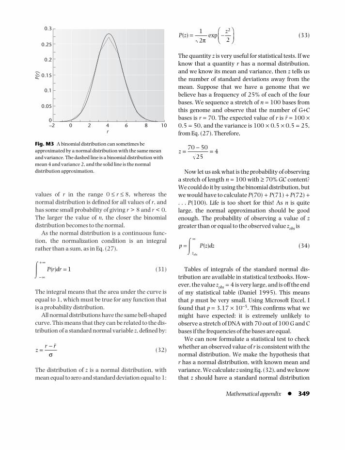
values of r in the range 0 ≤ r ≤ 8, whereas the normal distribution is defined for all values of r, andhas some small probability of giving r > 8 and r < 0.The larger the value of n, the closer the binomial distribution becomes to the normal.

As the normal distribution is a continuous func-tion, the normalization condition is an integralrather than a sum, as in Eq. (27).

(31)

The integral means that the area under the curve isequal to 1, which must be true for any function thatis a probability distribution.

All normal distributions have the same bell-shapedcurve. This means that they can be related to the dis-tribution of a standard normal variable z, defined by:

(32)

The distribution of z is a normal distribution, withmean equal to zero and standard deviation equal to 1:

z

r

=

− Rσ

�

−∞

+∞

= ( ) P r dr 1

(33)

The quantity z is very useful for statistical tests. If weknow that a quantity r has a normal distribution,and we know its mean and variance, then z tells usthe number of standard deviations away from themean. Suppose that we have a genome that we believe has a frequency of 25% of each of the fourbases. We sequence a stretch of n = 100 bases fromthis genome and observe that the number of G+Cbases is r = 70. The expected value of r is R = 100 ×0.5 = 50, and the variance is 100 × 0.5 × 0.5 = 25,from Eq. (27). Therefore,

Now let us ask what is the probability of observinga stretch of length n = 100 with ≥ 70% GC content?We could do it by using the binomial distribution, butwe would have to calculate P(70) + P(71) + P(72) +. . . P(100). Life is too short for this! As n is quitelarge, the normal approximation should be goodenough. The probability of observing a value of zgreater than or equal to the observed value zobs is

(34)

Tables of integrals of the standard normal dis-tribution are available in statistical textbooks. How-ever, the value zobs = 4 is very large, and is off the endof my statistical table (Daniel 1995). This meansthat p must be very small. Using Microsoft Excel, Ifound that p = 3.17 × 10−5. This confirms what wemight have expected: it is extremely unlikely toobserve a stretch of DNA with 70 out of 100 G and Cbases if the frequencies of the bases are equal.

We can now formulate a statistical test to checkwhether an observed value of r is consistent with thenormal distribution. We make the hypothesis that r has a normal distribution, with known mean andvariance. We calculate z using Eq. (32), and we knowthat z should have a standard normal distribution

p P z dz

zobs

( )=∞

�

z

=

−=

70 50

254

P zz

( ) exp= −⎛⎝⎜

⎞⎠⎟

1

2 2

2

π

Mathematical appendix l 349

0.15

0.2

0.3

0

0.05

0.1

0.25

2–2 0 4 6r

8 10

P(r)

Fig. M3 A binomial distribution can sometimes beapproximated by a normal distribution with the same meanand variance. The dashed line is a binomial distribution withmean 4 and variance 2, and the solid line is the normaldistribution approximation.

BAMZ01 09/03/2009 16:34 Page 349

if the hypothesis is true. The statistical tables tell usthat there is a probability of 2.5% that z > 1.96, andby symmetry, there is a probability of 2.5% that z < −1.96. Thus, there is a probability of 95% that zlies in the interval −1.96 ≤ z ≤ 1.96. We say that thehypothesis is rejected at the 5% level if the observedvalue of z lies outside this range. This is a two-tailedtest that rejects the hypothesis if z is either very highor very low. 5% is the probability that z is in one orother of the two tails of the distribution (see Daniel1995, if you need more details on this).

M.11 POISSON DISTRIBUTIONS

The Poisson distribution is a limiting case of thebinomial distribution that occurs when the numberof events n is extremely large, but the probability ofthe outcome of interest a is very small. The archety-pal example of this is radioactive decay. We have asample of a material containing n = 1023 radioactivenuclei. Each nucleus has a very small probability a = 5 × 10−23 of decaying per minute, and this isdetectable via a click on a Geiger counter. Let r be the number of clicks we count in one minute. Theprobability distribution of r is given by Eq. (26),

However, it is possible to derive a simplified for-mula for P(r) that applies in this case. The meannumber of clicks per minute is R = na, which is 5here. Typical values of r will be close to this value,whereas n is very much larger than this. As we known >> r, we can make the approximation

= n(n − 1)(n − 2) . . . (n − r + 1) ≈ nr

We can also use the approximation that

(1 − a)n ≈ e−na (35)

This approximation applies whenever n is large anda is small. In our case, e−5 = 6.74 × 10−3. If we set

n

n r

!( )!−

P r

n

r n ra ar n r( )

!!( )!

( )=−

− −1

n = 100 and a = 0.05, we get 0.95100 = 5.92 × 10−3,which is roughly 10% out. If n = 1000 and a = 0.005,we get 0.9951000 = 6.65 × 10−3, which is consider-ably closer. If we increase n and decrease a (keepingna = 5), the approximation gets closer and closer (trythis yourself with a calculator). For our original val-ues in the radioactivity problem, the approximationis almost exact. It is useful to define the parameter λ = na. If we now insert the two approximations intoEq. (26), we obtain

i.e., (36)

This result is the Poisson distribution. (Note that, inthe final step, we forgot about the (1 − a)−r as this isvery close to 1 in the limit we are interested in). ThePoisson distribution depends on a single parameter,λ, whereas the binomial distribution depends on twoparameters, n and a. It is worth remembering that thevariance of a Poisson distribution is equal to its mean λ.

Figure M4 shows a Poisson distribution with λ = 5, a binomial distribution with n = 50 and a = 0.1

P r

re

r( )

!= −λ λ

P r

n

ra e a

rr na r( )

!( )≈ −− −1

350 l Mathematical appendix

0.15

0.2

0.3

0

0.05

0.1

0.25

20 4 6r8 10 12 14 16

P(r)

Fig. M4 A binomial distribution tends to a Poisson distributionwhen n >> 1 but the mean value remains constant. Solid line:Poisson distribution with mean λ = 5. Dashed line: a binomialdistribution with n = 50 and a = 0.1. Dot-dashed line: abinomial distribution with n = 10 and a = 0.5.

BAMZ01 09/03/2009 16:34 Page 350

(which is quite close to the Poisson distribution), anda binomial distribution with n = 10 and a = 0.5(which also has a mean of 5, but is significantly different in shape from the Poisson distribution).

The Poisson distribution is relevant in the contextof genome sequencing. Suppose we have a genomeof total length L. We are sequencing many shortfragments, each of length l (which is very much less than L), and we will suppose these to be posi-tioned randomly within the genome. Consider oneparticular nucleotide in the genome. The probabil-ity that this falls within the range sequenced in anyone fragment is a = l/L. After n fragments have been sequenced, the probability that the particularnucleotide has been sequenced r times is given by abinomial distribution, defined by n and a. However,we are in the limit where we can approximate it by aPoisson distribution with λ = nl/L. Therefore,

(37)

M.12 CHI-SQUARED DISTRIBUTIONS

Let z1 . . . zk be k random numbers, each of which is drawn from a standard normal distribution P(z)(Eq. (33)). The quantity

(38)

has a probability distribution called a χ2 distribu-tion, with k degrees of freedom. The shape of this dis-tribution is:

(39)

In the above formula, Γ(k/2) is the gamma functiondiscussed in Section M.13 below. This is just a con-stant that normalizes the distribution in Eq. (39).

The importance of this distribution comes from itsuse in statistical tests. Here we will give two brief

P y

e y

k

yk

k( )

( / )

/

/=

− −2 21

22 2Γ

y zii

k

==∑ 2

1

P rnl

L

nl L

r

r

( ) exp( / )

!=

⎛⎝⎜

⎞⎠⎟

−

examples of the use of chi-squared tests on frequen-cies of bases in DNA (see Daniel 1995, if you needrefreshing on this).

In the small subunit ribosomal RNA gene from E.coli (EMBL accession number J01859), the observednumbers of bases of each type are given below. Theexpected number in brackets is calculated under thehypothesis that all four bases have equal frequency.

i n iobs(n i

exp )

A 389 (385.25)C 352 (385.25)G 487 (385.25)T 313 (385.25)

Total 1,541

We calculate the quantity X2 defined by

(40)

where the sum runs over the four types of base. Itcan be shown that X2 has a distribution that is veryclose to the χ2 distribution if the hypothesis is true.The number of degrees of freedom is 3 in this case (itis always one less than the number of categories).From statistical tables, the values of χ2 correspond-ing to p values of 5% and 1% are

0.05 0.01

1 d.o.f. 3.841 6.6352 d.o.f. 5.991 9.2103 d.o.f. 7.815 11.345

In this case, X 2 = 43.3. This is very much largerthan 11.345; therefore, the probability of observingthis distribution of bases in the gene if the bases haveequal frequency is very much less than 1%. Micro-soft Excel comes in handy again here: the probabilityof observing a value greater than or equal to 43.3 is2.1 × 10−9. Thus, there is a significant deviationfrom equal base frequencies.

Now let us compare the large subunit rRNA genefrom E. coli (EMBL accession number V00331) with

X

n n

niobs

i

ii

22

( )exp

exp=

−∑

Mathematical appendix l 351

BAMZ01 09/03/2009 16:34 Page 351

the small subunit gene. The observed numbers ofbases for the two genes are given below (mi for thelarge subunit and ni for the small subunit). Theexpected numbers are calculated under the hypo-thesis that the frequencies of the bases are the samein both genes. For example, the average frequency ofA is 1,151/4,445; therefore, the expected number ofA’s in the first gene is 1,541 × 1,151/4,445 = 399.0.

i n iobs(n i

exp) m iobs(m i

exp) Row totals

A 389 (399.0) 762 (752.0) 1,151C 352 (343.6) 639 (647.4) 991G 487 (485.0) 912 (914.0) 1,399T 313 (313.4) 591 (590.6) 904

Total 1,541 2,904 4,445

X2 is the sum of eight terms:

(41)

which adds up to 0.71. The number of degrees offreedom, when dealing with tables like this, is equalto (number of rows − 1) × (number of cols − 1),which is 3 × 1 = 3 in this case. From the table of χ2

values, 0.71 is much less than 7.81, hence the prob-ability of this distribution of bases occurring is

X

n n

n

m m

miobs

i

ii

iobs

i

ii

22 2

( )

( )exp

exp

exp

exp=

−+

−∑ ∑

greater than 5% (in fact p = 87% according to Excel).Therefore, we have no reason to reject the hypothesisthat the bases have the same frequency in the twogenes. We can say that the processes of mutation andselection acting on these genes cause a significant biasaway from equal base frequency, but that the sametypes of process seem to be working on both genes.

M.13 GAMMA FUNCTIONS ANDGAMMA DISTRIBUTIONS

The gamma function Γ(a) is defined by the integral

(42)

We can show directly from this that Γ(1) = 1, andΓ(2) = 1. Also, for any value of a

Γ(1 + a) = aΓ(a) (43)

Therefore, it follows that for an integer n

Γ(n) = (n − 1)! (44)

Another handy fact is that Γ(1/2) = π1/2. This,together with Eq. (43), allows us to calculate all

Γ( ) a x e dxa x=

∞− −�

0

1

352 l Mathematical appendix

2

3

4

5

0

1

6

0.2 0.4 0.6r

0.8 1.0 1.2 2.01.4 1.6 1.8

f (r,

a)

0.10.51

210100

Fig. M5 Gamma distributions f(r,a).Labels indicate the value of a on eachcurve.

BAMZ01 09/03/2009 16:34 Page 352

Mathematical appendix l 353

PROBLEMS

M1 In a card game, a player is dealt a hand of 13 cardsfrom the pack of 52. How many possible hands of 13cards are there? How many hands of cards are there thatcontain no aces? Hence, what is the probability that aplayer is dealt a hand with no aces?

In the same game, there are four players and eachreceives 13 cards. How many distinct ways are there ofdistributing the cards between the players?

M2 A genome contains 25% A, G, C, and T. What is theprobability that a 10-base stretch of DNA will have a GCcontent ≥ 70%?

M3 In a stretch of DNA of length n bases, we observe70% GC content. How long must the sequence bebefore we can reject the hypothesis that all bases haveequal frequency? Use an argument based on the zscore.

M4 The Drosophila genome is of length 180 Mb, and isto be sequenced in many short randomly positionedfragments of length 500 bases. How many fragmentsmust be sequenced so that the fraction of the genomethat has been missed by the random-sequencing pro-cess is less than 1%? What is the average number oftimes each base has been sequenced when this level ofcoverage is achieved?

the values Γ(3/2), Γ(5/2), etc. that occur in the chi-squared distribution (Eq. (39)).

The gamma distribution is a probability distribu-tion for a variable x that can take any positive valuebetween 0 and infinity. It is defined as

(45)

From the definition of Γ(a) in Eq. (42), we can seethat Eq. (45) is a properly normalized probability dis-tribution. In fact, Eq. (45) describes a whole family ofdistributions whose shapes are controlled by thevalue of a. The mean value of x is equal to a, with thedefinition above. It is useful to rescale the distribu-tion so that the mean is at 1. Defining a new variabler = x/a, and changing variables, we obtain

f x ax e

a

a x( , )

( )=

− −1

Γ

(46)

The shapes of the distributions f(r,a) for several val-ues of a are shown in Fig. M5. When a < 1, theweight of the distribution is close to r = 0 and there isa long tail extending to high r. When a = 1, the curveis a simple exponential. When a > 1, the distributionbecomes peaked around r = 1. For very large a, thecurve becomes a delta function. The mean value of ris 1 for all values of a.

REFERENCESCornish-Bowden, A. 1999. Basic Mathematics for Biochemists,

second edition. Oxford, UK: Oxford University Press.Daniel, W.W. 1995. Biostatistics: A Foundation for Analysis

in the Health Sciences, sixth edition. New York: Wiley.

f r aa r e

a

a a ar( , )

( )=

− −1

Γ

SELF-TESTMathematical background

For each of questions 1–4, which ofthe mathematical statements is correct?

C:

D:

13

14

512

+ =

13

14

112

− =1

A:

B:

13

14

17

+ =

13

14

112

+ =

BAMZ01 09/03/2009 16:34 Page 353

354 l Mathematical appendix

2A: log(2) + log(3) = log(5)B: log(8) = 3 log(2)C: log(8) = 8 log(1)D: log(2) + log(3) = log(8)

3A: 210 + 410 = 610

B: 210 + 26 = 216

C: 3 × 210 = 230

D: 8 × 210 = 213

4

A:

B:

C:

D:

5 In a class of 20 students, theteacher asks for two volunteers.How many different ways can thetwo volunteers be chosen?A: 220

B: 20 × 19C: 20 × 19/2D: 20!

6 The class of 20 students is havinga games lesson. How many differentways can the class be divided intotwo teams of 10?A: 20!B: 10! + 10!C: 20! / (10! × 10!)D: 20! / (2 × 10! × 10!)

7 The value of the definite integral

2xdx is

�

4

5

nn

n2

1

8

64=

=

∑ = !

nn n n

n

n2

1

81 2 16=

=

∑ =+ +

( )( )

n n nn

n

n

n

n

n2

4

82

1

82

1

3

=

=

=

=

=

=

∑ ∑ ∑= −

n n nn

n

n

n

n

n2

4

82

1

82

3

8

=

=

=

=

=

=

∑ ∑ ∑= −

D: P(n) is a bell-shaped curve with apeak at n = 50.

11 A DNA sequence of length 100is obtained from a real sequencedatabase. The numbers of the fourdifferent bases are:

A = 20; C = 27; G = 34; T = 19

The 5% significance values in the c2

table are

No. of degrees 5% significance of freedom value1 3.842 5.993 7.824 9.49

A: The c2 test shows that the content of G+C bases differssignificantly from 50%.B: The c2 test shows that the content of G+C bases does not differ significantly from 50%.C: More information is needed tocarry out a c2 test.D: A c2 test is not valid in this case.

12 A student answers a multiplechoice exam paper with 12questions on it. He guessesrandomly from the four possibleanswers on each question. Which of the following is true?A: The probability of guessing all 12 questions correctly is slightlygreater than 3%.B: The probability of getting exactlythree correct answers is 0.0156.C: The probability of getting exactly three correct answers is 1.17 × 10−3.D: The probability of guessing allanswers wrong is greater than theprobability of guessing all answersright.

A: 9B: 5C: 2D: 1

8 Which of the functions f(x) is asolution of the following differentialequation?

A:

B:

C: f(x) = e2 + 1/2D: f(x) = ex + 1/2

9 A solution contains many RNAoligomers of length six bases. Allfour bases are present with equalfrequency and are present inrandom orders in the oligomers.The proportion of oligomerscontaining exactly two guaninesshould be approximately:A: 0.2966B: 0.0625C: 0.0198D: 0.000244

10 A DNA sequence of length 100nucleotides is generated randomlysuch that each of the four bases A,C, G, and T is chosen with equal frequency. The base at eachposition is chosen independently of the others. Let P(n) be theprobability that there are n Gs in thesequence. Which of the followingstatements is correct?A: P(n) can be approximated by anormal distribution with mean 20and variance 75.B: P(n) can be approximated by anormal distribution with mean 25and variance 18.75.C: P(n) can be approximated by aPoisson distribution with mean 25and variance 25.

f x e x( ) = +

12

12

f x e x( ) ( )= +

12

12

dfdx

f = −2 1

BAMZ01 09/03/2009 16:34 Page 354

List of Web addresses

PROTEIN FAMILY

PROSITE http://www.expasy.org/prosite/PRINTS http://www.bioinf.man.ac.uk/

dbbrowser/PRINTS/Blocks http://blocks.fhcrc.org/Profiles http://hits.isb-sib.ch/cgi-bin/

PFSCAN/Pfam http://www.sanger.ac.uk/Software/

Pfam/eMOTIF http://fold.stanford.edu/emotif/InterPro http://www.ebi.ac.uk/interpro/

PROTEIN STRUCTURE

PDB http://www.rscb.org/pdb/SCOP http://scop.mrc-lmb.cam.ac.uk/scop/CATH http://www.biochem.ucl.ac.uk/bsm/

cath/PDBsum http://www.biochem.ucl.ac.uk/bsm/

pdbsum/CDD http://www.ncbi.nlm.nih.gov/

Structure/cdd/cdd.shtml

METABOLIC/PATHWAY

KEGG http://www.genome.ad.jp/WIT http://www-wit.mcs.anl.gov/Gongxin/EcoCyc http://ecocyc.org/UMBBD http://umbbd.ahc.umn.edu/

List of Web addresses l 355

NUCLEOTIDE SEQUENCE

EMBL http://www.ebi.ac.uk/embl/GenBank http://www.ncbi.nlm.nih.gov/

GenBank/DDBJ http://www.ddbj.nig.ac.jp/INSD http://www.ncbi.nlm.nih.gov/

projects/collab/dbEST http://www.ncbi.nlm.nih.gov/

dbEST/UniGene http://www.ncbi.nlm.nih.gov/

UniGene/

ORGANISM

FlyBase http://flybase.bio.indiana.edu/SGD http://yeastgenome.org/WormBase http://www.wormbase.org/MGD http://www.informatics.jax.org/TAIR http://www.arabidopsis.org/Ensembl http://www.ensembl.org/TDB http://www.tigr.org/tdb/

PROTEIN SEQUENCE

PIR http://pir.georgetown.eduMIPS http://mips.gsf.de/Swiss-Prot http://www.expasy.org/sprotNRL-3D http://www-nbrf.georgetown.edu/

pirwww/dbinfo/nrl3d.htmlUniProt http://www.uniprot.org/

BAMZ02 09/03/2009 16:33 Page 355

OTHER

OMIM http://www3.ncbi.nlm.nih.gov/entrez/query.fcgi?db=OMIM

BIND http://www.blueprint.org/bind/bind.php

GO http://www.geneontology.org/NAR http://nar.oupjournals.org/DBcat http://www.infobiogen.fr/services/

dbcat

356 l List of Web addresses

BAMZ02 09/03/2009 16:33 Page 356

Glossary

base chemical group that is part of a nucleotide.May be either a purine or a pyrimidine. The sequ-ence of bases in a nucleic acid stores the informationcontent.BLAST (Basic Local Alignment Search Tool) awidely used program for searching sequence data-bases for entries that are similar to a specified querysequence.BLOSUM (BLOcks SUbstitution Matrix) type ofamino acid scoring matrix (derived from blocks in the Blocks database) used in aligning proteinsequences.bootstrapping a statistical technique used toestimate the reliability of a result (usually a phylo-genetic tree) that involves sampling data withreplacement from the original data set.cDNA DNA strand that is complementary to anRNA strand and synthesized from it by a reversetranscriptase.chloroplast (also called plastid) an organelle ineukaryotes such as plants and algae that possessesits own genome and is responsible for photosyn-thesis. Thought to have arisen by the incorporationof a cyanobacterium into an ancient eukaryotic cell(cf. endosymbiosis).clade a group of species including all the speciesdescending from an internal node of a tree and noothers.coalescence the process by which the lines ofdescent of individuals or sequences in a present-daypopulation converge towards a single commonancestor at some point in the past.codon triplet of three nucleotides that specifies

Glossary l 357

accession number a unique identifier for a data-base entry (e.g., a protein sequence, a protein familysignature) that is assigned when the entry is origin-ally added to a database and should not changethereafter.advantageous mutation a mutation that causesthe fitness of a gene to be increased with respect tothe original sequence.algorithm a logical description of the way to solvea given problem that could be used as a specificationfor how to write a computer program.alignment an arrangement of two or moremolecular sequences, one below the other, such thatregions that are identical or similar are placed imme-diately below one another.allele one of several alternative sequences for aparticular gene present in a population.annotation (i) text in a database entry (e.g., for a gene sequence) that describes what the entry is (including relevant background information, literature references, and cross-references to otherdatabases) to a human reader; (ii) the process ofassigning readable explanations to all the entries ina database (e.g., the complete set of gene sequencesin a genome).archaea one of three principal domains of life.Archaeal cells can be distinguished from bacterialcells based on gene sequence and gene content.Many archaea are specialized to conditions ofextreme heat or salinity.bacteria (singular bacterium) one of three prin-cipal domains of life. Bacterial cells contain no nucleusand usually possess a cell wall of petidoglycan.

BAMZ03 09/03/2009 16:32 Page 357

one type of amino acid during the translation process.codon usage the frequency with which eachcodon is used in a gene or genome, particularly therelative frequencies with which synonymous codonsare used.compensatory substitutions a pair of substitu-tions at different sites in a sequence such that eachone alone would be deleterious, but are neutralwhen both occur together (e.g., in RNA helices).complementary sequences two nucleic acidsequences that can form an exactly matching dou-ble strand as a result of A-T and C-G pairing. Com-plementary sequences run in opposite directions:ACCAGTG is complementary to CACTGGT.deleterious mutation a mutation that causesthe fitness of a gene to be reduced with respect to theoriginal sequence.dynamic programming a type of algorithm inwhich a problem is solved by building up fromsmaller subproblems using a recursion relation (e.g.,in sequence alignment and RNA folding).electrophoresis method of separating chargedmolecules according to their rate of motion througha gel under the influence of an applied electric field.endosymbiosis process by which a bacterial cellwas enclosed within a eukaryotic cell and eventu-ally became an integral part of the cell. Thought tohave given rise to chloroplasts and mitochondria.eukaryotes one of three principal domains of life.Eukaryotic cells possess a nucleus, and usually con-tain other organelles like, e.g., mitochondria, endo-plasmic reticulum, Golgi apparatus, a cytoskelton ofactin and tubulin.exon part of a gene sequence that is transcribedand translated to give rise to a protein (cf. intron).fixation the spread of an initially rare mutantallele through a population until it becomes themost frequent allele for that gene.gap a space in a sequence alignment indicatingthat a deletion has occurred from the sequence con-taining the gap, or that an insertion has occurred inanother sequence.gap penalty (or gap cost) part of the scoring sys-tem used for sequence alignments intended to penal-ize the insertion of unnecessary gaps.

generalize the ability of a supervised learningalgorithm (e.g., a neural network) to perform wellon data other than that on which it was specificallytrained.genetic code set of assignments of the 64 codonsto the 20 amino acids.genome the complete sequence of heritable DNAof an organism.genomics the study of genomes. Usually appliesto studies that deal with very large sets of genesusing high-throughput experimental techniques.global alignment an alignment of the whole ofone sequence with the whole of another sequence.heuristic algorithm an algorithm that usuallyproduces fairly good answers most of the time, butcannot be proven to give the best answer all thetime.hidden Markov model a probabilistic model of a protein sequence alignment in which the probab-ility of a given amino acid occurring at a given sitedepends on the value of hidden variables in themodel.high-throughput experiments experimentsthat allow large numbers of genes or gene productsto be studied at the same time using partially auto-mated methods.homologs sequences that are evolutionarily re-lated by descent from a common ancestor (cf.orthologs and paralogs).horizontal gene transfer the acquisition of agene from an unrelated species by incorporation of“foreign” DNA into a genome.hybridization the binding of a nucleic acidstrand to its complementary sequence.hydrophobic an amino acid is said to be hydro-phobic if its free energy would be higher when incontact with water than when buried in the interiorof a protein, i.e., it would “prefer” not to be in contactwith water. In contrast, a hydrophilic amino acidwould “prefer” to be in contact with water.IEF (isoelectric focusing) technique for separatingproteins from one another according to the value oftheir pI (isoelectric point). Used as the first dimen-sion in 2D gel electrophoresis.indel an insertion or deletion occurring in a pro-tein or nucleic acid sequence. The term denotes the

358 l Glossary

BAMZ03 09/03/2009 16:32 Page 358

fact that we do not know whether a gap in asequence is actually a deletion in that sequence oran insertion in a related sequence.interactome the complete set of protein–proteininteractions that occurs in a cell.intron part of the DNA sequence of a gene that istranscribed, but is cut out of the mRNA (i.e., spliced)prior to translation. Introns do not code for proteinsequences.knowledge-based an approach that uses infor-mation from previously known examples in order tomake predictions about new examples. Used in con-trast to an ab initio approach, in which a predictionwould be made based on a fundamental theory orprinciple.local alignment an alignment of a part of onesequence with a closely matching part of anothersequence.locus a position on a chromosome correspondingto a gene or a molecular marker used in populationgenetics studies.log-odds a quantity that is calculated as the loga-rithm of the relative likelihood of an event to its like-lihood under a null model. A positive log-odds scoreindicates that the event is more likely than it wouldbe under the null model.machine learning an approach in which a com-puter program learns to solve a problem by progress-ive optimization of the internal parameters of thealgorithm.MALDI (Matrix-Assisted Laser Desorption/Ionization) mass spectrometry technique used tomeasure the masses of peptide fragments.metabolome the complete set of chemicals in acell that are involved in metabolic reactions.microarray a glass slide or silicon chip ontowhich spots of many different DNA probes have beendeposited. Used for the simultaneous measurementof gene-expression levels of many genes in the sametissue sample.mitochondrial Eve hypothetical female fromwhom all present-day human mitochondrial DNA isdescended.mitochondrion (plural mitochondria) an organ-elle in eukaryotic cells that possesses its own genomeand is the site of aerobic respiration. Thought to

have arisen as a result of the incorporation of an α-proteobacterium into an ancient eukaryote (cf.endosymbiosis).monophyletic adjective describing a group ofspecies on a phylogenetic tree that share a commonancestor that is not shared by species outside thegroup. A clade is a monophyletic group.motif characteristic sequence of conserved orpartly conserved amino acids appearing in a proteinsequence alignment that can be used as a diagnosticfeature of a protein family.Muller’s ratchet the accumulation of deleteriousmutations in asexual genomes via a stochastic pro-cess that is virtually irreversible.nested models two probabilistic models suchthat the simpler one is a special case of the morecomplex one.neural network a type of machine-learning pro-gram used for pattern recognition, composed of anetwork of connected neurons.neuron an element of a neural network havingseveral inputs and one output. The output is a simplefunction of the combined inputs.neutral mutation a mutation whose fitness isequal to the fitness of the original sequence, orwhose fitness is sufficiently close to that of the ori-ginal sequence that the fate of the mutation is determined by random drift rather than naturalselection.normalize for a probability distribution, to divideall probabilities by a constant factor so that the sumof probabilities over all possible alternatives adds up to 1. For microarray data, to adjust the meas-ured intensities in order to correct for biases in theexperiment.nucleic acid a polymeric molecule composed ofnucleotides. May be either DNA (deoxyribonucleicacid) or RNA (ribonucleic acid).nucleotide chemical unit that forms the buildingblock for nucleic acids. Composed of a nitrogenousbase, a ribose or deoxyribose sugar, and a phosphategroup (cf. nucleic acid, purines, pyrimidines).null model a simple model used for calculatingthe probabilities of events that ignores factorsthought to be important. If the observed data differsignificantly from expectations under the null

Glossary l 359

BAMZ03 09/03/2009 16:32 Page 359

model, it can be concluded that the additional fac-tors are necessary to explain the observation.oligonucleotide a nucleic acid fragment com-posed of a small number of nucleotides.ontology specification of the set of terms and concepts used in a domain of knowledge givingdefinitions of the terms and relationships betweenthem.ORF (open reading frame) a continuous sequenceof DNA in a genome beginning with a start codonand ending with a stop codon in the same tripletreading frame that could potentially be a protein-coding gene.organelle structural component of a eukaryoticcell.orthologs sequences from different species thatare evolutionarily related by descent from a com-mon ancestral sequence and that diverged from oneanother as a result of speciation.outgroup a species (or group of species) that isknown to be the earliest-diverging species in a phylo-genetic analysis. The outgroup is added in order todetermine the position of the root.PAGE (polyacrylamide gel electrophoresis) tech-nique for separating proteins from one anotheraccording to their molecular weight.PAM (point accepted mutation) matrix a matrixdescribing the rate of substitution of one type ofamino acid by another during protein evolution.paralogs sequences from the same organism thathave arisen by duplication of one original sequence.parsimony a principle that states that the sim-plest solution to a problem (or the solution using thefewest arbitrary assumptions) is to be preferred. Inmolecular phylogenetics, the tree that requires thefewest mutations is preferred.pathogenicity island region of a bacterial gen-ome containing genes responsible for the patho-genic behavior of some strains of bacteria. The islandis usually not present in all strains of the species andis thought to have been acquired by horizontaltransfer.PCA (principal component analysis) technique forvisualizing the relationship between points in a multi-dimensional data set in a small number of dimen-sions (usually two or three).

PCR (polymerase chain reaction) experimentaltechnique by which a specified sequence of DNA ismultiplied exponentially by repeated copying andsynthesis of both complementary strands.perceptron simplest type of neural network, hav-ing only a single layer of neurons.peptide a sequence of amino acids connected in achain via peptide bonds. Usually refers to a sequenceof a few tens of amino acids, in contrast to a protein,which usually contains a few hundred amino acids.phylogeny an evolutionary tree showing the rela-tionship between sequences or species.polymorphism the presence of more than oneallele for a given gene at an appreciable frequency ina population.polynomial time for a problem with input data ofsize N, a polynomial time algorithm will run in atime of order Nα, for some constant α. If α is small,the algorithm is efficient, and will work for largesized problems.polyphyletic adjective describing a group ofspecies on a phylogenetic tree for which there is nocommon ancestor that is not also shared by speciesoutside the group. A polyphyletic group is evolution-arily ill-defined.posterior in Bayesian statistical methods, the prob-ability of an event estimated after taking account ofthe information in the data (cf. prior).primary structure refers to the chemical struc-ture of a protein or nucleic acid. As far as bioinform-atics is concerned, this is just the sequence of theamino acids or bases in the molecule.primer short nucleic acid sequence that is used toinitiate the process of DNA synthesis from a specifiedposition, e.g., during PCR.prior in Bayesian statistical methods, the prob-ability of an event estimated from expectationsbased on previous experience, but before takingaccount of the information in the data to be analyzed(cf. posterior).prokaryotes cells lacking a nucleus. Thought tobe divided into two principal groups: archaea andbacteria.promoter region of DNA upstream of a gene thatacts as a binding site for a transcription factor andensures that the gene is transcribed.

360 l Glossary

BAMZ03 09/03/2009 16:32 Page 360

proteome the complete set of proteins present in acell.proteomics the study of the proteome, usuallyusing two-dimensional gel electrophoresis and massspectrometry to separate and identify the proteins.purines the bases A (adenine) and G (guanine)that are present in nucleic acid sequences.pyrimidines the bases C (cytosine), T (thymine),and U (uracil) that are present in nucleic acidsequences.random drift change in gene frequency owing tochance effects in a finite sized population rather thanto natural selection.redundant gene a gene that is not necessary tothe organism owing to the presence of another copyof the same gene or of another gene performing thesame function.regular expression a way of representing a sequ-ence of conserved or partly conserved amino acids ina protein motif.ribosome the organelle that carries out proteinsynthesis. Composed of small and large subunitRNAs and a large number of ribosomal proteins.ribozyme an RNA sequence that functions as acatalyst (by analogy with an enzyme, which is a pro-tein that functions as a catalyst).root the earliest point on an evolutionary tree.The common ancestor from which all species on thetree have evolved.rooted tree an evolutionary tree in which theroot is marked, and in which time proceeds from theroot towards the tips of the tree. In contrast, anunrooted tree does not specify the direction in whichtime is proceeding.schema specification of the types of object in adatabase, the attributes they possess, and the rela-tionship between the objects. A diagram represent-ing this specification.secondary structure elements of local structurefrom which the complete tertiary structure of a mole-cule is built. In proteins, the α helices and β strands.In RNA, the pattern of helical regions and loops.selectivity the proportion of objects identified bya prediction algorithm that are correct predictions.Selectivity = True Positives/(True Positives + FalsePositives).

sensitivity the proportion of the true members ofa set that are correctly identified by a prediction algo-rithm. Sensitivity = True Positives/(True Positives +False Negatives).stabilizing selection when natural selectionacts to retain ancestral sequences or characters andhence slows down the rate of evolutionary change.stacking interaction between one base pair andthe next in a double-stranded helix of RNA or DNA.substitution the replacement of one type ofnucleotide in a DNA sequence by another typeowing to the occurrence of a point mutation and thesubsequent fixation of this mutation in the popula-tion. Also the replacement of one type of amino acidin a protein by another type.supervised learning a learning procedure wherea program is given a set of right and wrong examplesand is trained to give optimum performance on thisset. In contrast, an unsupervised learning algorithmuses an optimization procedure without being givenexamples.synapomorphy a shared derived character inparsimony analysis that marks a group of species asevolutionarily related.synonymous substitution a substitution at thenucleic acid level that does not lead to change of theamino acid sequence of the protein (because of re-dundancy in the genetic code). A non-synonymoussubstitution is one that does change the amino acid.symbiont an organism that lives with anotherorganism of a different species in a mutually bene-ficial way.TAP (tandem affinity purification) technique forsimultaneously isolating sets of proteins that inter-act in the form of complexes.taxon (plural taxa) name for a group of speciesdefined in a hierarchical classification.tertiary structure the complete three-dimen-sional structure of a molecule, such as a protein or RNA, built from the packing of its secondarystructures.Test set a set of known examples used for verify-ing the performance of an algorithm (e.g., a neuralnetwork). The test set must be distinct from thetraining set.

Glossary l 361

BAMZ03 09/03/2009 16:32 Page 361

training set a set of known examples on whichan algorithm (e.g., a neural network) is trained. Thealgorithm is optimized to give the best possibleresults on the training set.transcription the synthesis of an RNA strandusing a complementary DNA strand as a template.transcription factor a protein that binds to aregulatory region of DNA, usually upstream of thecoding region, and influences the rate of transcrip-tion of the gene.transcriptome the complete set of mRNAs tran-scribed in a cell.

transition in the strict sense, the substitution of apurine by another purine, or of a pyrimidine byanother pyrimidine. In the more general sense, anysubstitution in a DNA sequence, and sometimes alsoused for substitutions of amino acids.translation the process by which the ribosomedecodes the gene sequence specified on a mRNA andsynthesizes the corresponding protein.transversion the substitution of a purine by apyrimidine or vice versa (cf. transition).yeast two-hybrid experimental technique fordetermining whether a physical interaction occursbetween two proteins.

362 l Glossary

BAMZ03 09/03/2009 16:32 Page 362

dbCAT 81, 114dbEST 87DDBJ 1, 88Dirichlet distribution 232–3distance matrix 30, 132DNA

replication 21–2structure 12–13

dynamic programming 123–7, 238,260–4

EBI 84EcoCyc 114electrophoresis 5, 51, 325–6EMBL database 1, 84–5eMOTIF 95–6, 108endosymbiosis 298–300Ensembl 114Entrez 85ESTs 84, 85, 87Escherichia coli 291–4eukaryotes (evolution of ) 277–8,

298–301E values 139–41, 145–7, 153–4evolution (definition) 37–8ExPASy 93, 105Expectation-maximization algorithm

237extreme value distribution 149–53

false positives/false negatives 146FASTA (file format) 83

(program) 143–7feature table 85, 92file formats 82–111fingerprints 95–6, 200–5, 213–14

breakpoint distance 306–8Buchnera 288–9, 295

Captain Kirk 143–4CASP 252CATH 113CDD 114central dogma 16–22chloroplasts 298–300, 303clade 161ClustalX/ClustalW 128, 132–5clustering

direct 33hierarchical 28–33K-means 33microarray data 320–2phylogenetics 162–9

coalescence 44–6codon bias 53–4, 292codons 19–20, 42, 53–4COGs 294–6coiled coils 237–8color blindness 210compensatory substitutions 258–9,

265cones 209consensus trees 170, 184–5correlation coefficient 28, 30

database accession numbers 82, 92, 97, 98,

99, 102, 104, 110divisions 84ID codes 82, 92, 97, 99, 101, 102,

105data explosion 1–7, 11

adaptation/adaptationist 49–53additive trees 166, 171algorithms 119–21alignment

global 123local 125multiple 130–6pairwise 121–30progressive 130–5statistics 147–55

alleles 7, 39, 51, 56allozymes 51amino acids

physico-chemical properties22–32, 72–4, 245

relative mutability 68–9, 72structure 14–15

aminoacyl-tRNA synthetase 20, 293anticodon 20, 56–7archaerhodopsin 208Archezoa 301Atlas of Protein Sequence and Structure

89

Back-propagation 249Baum–Welch algorithm 237Bayesian methods 180–5, 229–33bacteriorhodopsin 208–9BIND 114bioinformatics (definition) 6BLAST 143–7, 153–5, 195Blocks (database) 75, 95–6, 102–4

(motifs) 95–6, 205–7BLOSUM matrices 74–5, 147, 196bootstrapping 169–71BRCA1 40–3

Index

Index l 363

BAMZ04-Index 09/03/2009 16:32 Page 363

Fitch–Margoliash method 171fitness 38, 48–9fixation 46–50, 56flatfiles 83FlyBase 114forward and backward algorithms

239

G protein-coupled receptors 208–16G protein coupling 215–16gamma distribution 64, 175, 352gap penalties 122, 126–7, 134G–C skew 290GenBank 1–4, 85–7, 154gene content phylogenies 296–8gene deletion 288, 304–5gene duplication 131, 290–1,

304–5gene ontology 110–11, 335–6gene order phylogenies 305–9general reversible model 63generalization (in neural networks)

245, 248genetic code 19–20, 73genomics 5–6, 313–14gradient descent/ascent 248GSSs 84, 85

halorhodopsin 208Hasegawa, Kishino, and Yano (HKY)

model 63, 175hexokinase 70, 128–34, 294hidden Markov models 95–6,

234–43high-throughput techniques 5,

313–30hill-climbing algorithm 173, 181homologs/homology 8, 161, 209homoplasy 177horizontal gene transfer 290–4HTCs 84, 85HTGs 84, 85hydrophobicity 24–5

indels 40informative sites 45, 178, 187INSD 88InterPro 108–11, 141–2intron/exon 41inversions 288, 304

ISI Science Citation Index 5–6ISREC 96, 105

JIPID 88, 89Jukes–Cantor model 60–2, 162

KEGG 114Kimura two-parameter model 63

life (definition) 37ligand binding (of GPCRs) 215–16likelihood ratio test 267–70log-odds scores 71–5, 229long-branch attraction 179, 277,

301

machine learning 227–8, 323–5mammals 42–3, 162–9, 175–85,

272–6Markov Chain Monte Carlo 181–5,

232, 307Markov model 234mass spectrometry 5, 326maximum likelihood 173–6,

178–81MEDLINE 85metazoa 276–7, 307–8Metropolis algorithm 181MGD 114MIAME standard 332microarrays 5–6, 314–25microsatellites 40MIPS 90mitochondrial DNA/mitochondrial

Eve 44–5mitochondrial genomes 298–309model selection 266–70molecular clock 165, 275–6Moore’s law 2–4motifs 96, 99–102, 197, 204MPsrch 139–42mutations 39–43

NCBI 85nearest neighbor interchange 171–2Needleman–Wunsch algorithm

123–5neighbor joining 132, 166–9, 187neural networks 244–53neutral evolution 38, 41–7, 49–54

normalization 316–19NRL3D 94–5nucleic acid (see DNA and RNA)

’omes (definitions) 313–14OMIM 90, 114ontologies 334–6open reading frames 286opsins 210–11orthologs 209–10, 291, 294outgroup 160

PAGE (see electrophoresis)PAM model

derivation 65–72distances 69–72scoring matrices 71–4, 139–42,

147, 196, 202, 270paralogs 209–10, 294parsimony 65–6, 177–9, 187, 306pathogenicity islands 291–2pattern recognition 227–8PCR 22–3PDB 3, 111–12PDBsum 113peptide mass fingerprinting 326perceptron 246–7Pfam 95–6, 107–8, 243pI 24–5, 325–7PIR 89, 94–5PIR SUPERFAMILY 109polymorphism 39, 45position-specific scoring matrix

144–5, 196, 205–8principal component analysis 25–9,

322–3PRINTS 95–6, 98–102, 213–14prion proteins (in databases) 96–111prior/posterior probabilities 180,

229–33ProDom 107, 109profiles 95–6, 105–7, 196, 205–8,

231profile HMM 241–3prokaryotic genomes 283–98PROSITE 95–8, 197–200, 219–21protein

folding 14, 20–5structure 14–16structure prediction 250–3

364 l Index

BAMZ04-Index 09/03/2009 16:32 Page 364

protein family databases 95–111,197–208

protein–protein interaction network330

protein structure databases 111–13protein tyrosine phosphatase

139–42, 145, 154proteobacteria 284–94proteomics 5–6, 325–30pseudocounts 231PSI–BLAST 144–5PubMed 85

quartet puzzling 179–80

random drift 38, 47–50Reclinomonas americana 299–300recombination 46regular expressions 95–7, 198–200replicator 38restriction fragment length

polymorphism 51Rhizobia 289–90rhodopsin 209–11ribosome 21ribozyme 21Rickettsia 284–5, 288–9, 300rods 209rooted/unrooted trees 158–61, 166RNA

free energy parameters 263–4processing/splicing 18rRNA 21, 162, 257–8structure 13–14, 257–66tRNA 14, 54, 56–7, 307–8

rules (regular expression) 198–9

SCOP 112selection 48–54

selective sweep 49, 53self-organizing map 323–4sensitivity and selectivity 146sensory rhodopsin 208sequence alignment (see alignment)serpentine receptors 209SGD 114Shakespeare 124–7, 131–2SIB 90signal peptides 250, 302single nucleotide polymorphism 10,

52SMART 109, 111Smith–Waterman algorithm 126,

139–42, 153sorting 119–20sparse matrix 201, 202splicing 18, 41SRS 85STSs 84, 85substitution rate matrices 58–64,

264–7SUPERFAMILY 109supervised/unsupervised learning

236, 244support vector machines 324–5Swiss–Prot 85, 90–3, 139–42, 145,

154, 221–5synapomorphy 177synonymous/non-synonymous

substitutions 40, 53, 56–7,271–2

TAIR 114tandem affinity purification 330–1Taq polymerase 23T–Coffee 135–6TDB 114TIGRFAMs 109

time reversibility 63top 500 supercomputers 2–4training set/test set 228, 244transcription 16–18transfer of genes from organelles to

the nucleus 301–4transition/transversion 39, 42,

63translocations 288, 304transmembrane helices 208–10,

215, 225, 229, 240–1traveling salesman problem 120–1tree optimization criteria 171tree space 171–3TrEMBL 85, 93, 223–4

ultrametricity 169UM–BBD 114unified modeling language 332–4UniGene 114UniProt 95untranslated regions 18UPGMA 164–6, 187

variability of rates between sites 64,175

visual pigments 209–10Viterbi algorithm 238, 242

WD-40 repeats 105–6WIT 114wobble 20WormBase 114Wright–Fisher model 47–50

Y chromosome 44–5yeast two-hybrid 328–9

z score 148, 349

Index l 365

BAMZ04-Index 09/03/2009 16:32 Page 365

BAMZ04-Index 09/03/2009 16:32 Page 366

BAMZ04-Index 09/03/2009 16:32 Page 367

BAMZ04-Index 09/03/2009 16:32 Page 368

BAMZ04-Index 09/03/2009 16:32 Page 369

BAMZ04-Index 09/03/2009 16:32 Page 370

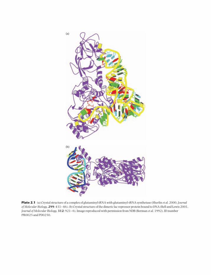
Plate 2.1 (a) Crystal structure of a complex of glutaminyl tRNA with glutaminyl-tRNA synthetase (Sherlin et al. 2000, Journalof Molecular Biology, 299: 431–46). (b) Crystal structure of the dimeric lac repressor protein bound to DNA (Bell and Lewis 2001,Journal of Molecular Biology, 312: 921–6). Image reproduced with permission from NDB (Berman et al. 1992). ID numberPR0025 and PD0250.

(a)

(b)

BAM_Plate Section 09/03/2009 16:27 Page 1

Plate 2.2 (a) Hierarchical clustering of the amino acids performed using CLUTO (Karypis 2000, University of Minnesotatechnical report #02–017), as described in Section 2.6.2. (b) Where clusters fail: the Venn diagram illustrates the overlappingproperties of amino acids. The color scheme is the one implemented in the CINEMA sequence alignment editor (Parry-Smith et al.1998, Gene, 221: GC57–GC63): red for acidic; blue for basic; green for polar neutral; purple for aromatic; black for aliphatic;yellow for cysteine (disulfide potential); and brown for proline and glycine (which have unique structural properties, especially inhelices).

(a)

(b)

BAM_Plate Section 09/03/2009 16:27 Page 2

Pla

te 3

.1T

he

patt

ern

of b

ases

obs

erve

d at

info

rmat

ive

site

s in

hu

man

mit

och

ondr

ial g

enom

es fr

om m

any

diffe

ren

t eth

nic

gro

ups

an

dth

e ph

ylog

enet

ic tr

ee d

edu

ced

from

this

info

rmat

ion

. Rep

rodu

ced

from

Ingm

an et

al.

(20

00

, Nat

ure,

40

8: 7

08

–13

), w

ith

per

mis

sion

from

Nat

ure

Pu

blis

hin

g G

rou

p.

BAM_Plate Section 09/03/2009 16:27 Page 3

(b)

OPSD_SHEEP

OPSD_BOVINOPSD_MOUSEOPSD_HUMANOPSD_XENLAOPSD_CHICKOPSD_LAMJA

OPSG_CHICKOPSG_CARAU

OPSB_GECGE

OPSU_BRARE

(c)

OPSG_GECGE

OPSG_ASTFA

OPSG_HUMAN

OPSR_HUMAN

OPSR_ANOCA

OPSR_CHICK

OPSR_ASTFA

OPSR_CARAU

(a)

Plate 9.1 (a) Logo for the prion block depicted in Fig. 9.3. The completely conserved glycine and highly conserved prolineresidues that form the GPG anchor for this block are clearly visible toward the center of the logo. (b) Excerpts from sequencealignments of vertebrate visual receptors. The coloring of the amino acids follows the scheme shown in Plate 2.2(b). Part of thetypical signature of rhodopsin (denoted OPSD) sequences is shown. (c) Part of the typical signature of red/green opsins (denotedOPSR and OPSG). Note that the red and green sequences are highly similar, such that it is almost impossible to separate themusing typical sequence analysis methods – the central motif, N-P-G-Y-[AP]-[FW]-H-P-L, which includes a conserved histidine, isparticularly striking. More startling is the fact that within the rhodopsin alignment are several “rogue” sequences, namely ofgreen, blue (OPSB), and purple (OPSU) opsins, that more closely resemble the rhodopsin sequence signature than they do theirown pigment sequences – in particular, the chicken (CHICK) and goldfish (CARAU) green pigments do not contain the N-P-G-Y-[AP]-[FW]-H-P-L motif characteristic of green sequences.

BAM_Plate Section 09/03/2009 16:27 Page 4

yvaQ

yvbJ

3,475,0003,450,001

yvaJ

yvbA

ABC transporters ABC transporters

similar to arsenical resistance operon repressor

1

0

Plate 10.1 Application of a three-state M1–M2 model to the Bacillus subtilis genome reveals an atypical segment (3,463–3,467 kb,underlined) surrounded by ABC transporter gene duplication (thin black arrows). Filled arrows represent genes of knownfunction, empty arrows, those of unknown function, and red hairpins represent transcriptional terminators. The colored curvesshow the probabilities of being in each of the three hidden states at each point in the sequence. The magenta state matches geneson the (+) strand, whereas cyan matches genes on the (−) strand. The black state fits either intergenic regions or atypical genes.Reproduced from Nicolas et al. (2002, Nucleic Acids Research, 30: 1418–26) with permission of Oxford University Press.

BAM_Plate Section 09/03/2009 16:27 Page 5

Plate 11.1 The secondary structure of SSU rRNA in E. coli. The color scheme shows the degree of variability of the sequenceacross the bacterial domain. Category 0 (purple) sites are completely conserved. Categories 1 to 5 range from very slowly evolving (blue) to rapidly evolving (red). The gray sites are present in less that 25% of the species considered, hence no measure of evolutionary rate was made. Reproduced with permission from the European Ribosomal RNA databasehttp://oberon.fvms.ugent.be:8080/rRNA/index.html

BAM_Plate Section 09/03/2009 16:27 Page 6

Plate 12.1 The genome of Rickettsia conorii, reproduced from Ogata et al. (2001), Copyright 2001 AAAS. (a) The outer circlegives the nucleotide positions in bases measured anticlockwise from the origin of replication. The second and third circles showthe positions of ORFs on the plus and minus strands, respectively. The colors used indicate different functional classes of gene. Thearrows in the fourth and fifth circles show the positions of tRNA genes, and the three black arrows show rRNAs. The sixth andseventh circles indicate short repeated sequences. The eighth circle shows G–C skew. The genome is found to be largely colinearwith R. prowazekii, except for the shaded sector on the lower left. (b) Three distinct regions of the R. conorii genome aligned withhomologous regions of the R. prowazekii genome. Most of the genes are present in the same order in both species. The top andmiddle sections show split genes in R. prowazekii and R. conorii, respectively. The bottom section contains a non-coding region ofR. prowazekii that shows some sequence similarity to a functional gene (rOmpA) in R. conorii.

(a)

(b)

BAM_Plate Section 09/03/2009 16:27 Page 7

Plate 12.2 Comparisons of gene order in pairs of animal mitochondrial genomes constructed using the OGRe database(Jameson et al. 2003, Nucleic Acids Research, 31: 202–6). http://ogre.mcmaster.ca

BAM_Plate Section 09/03/2009 16:27 Page 8

OCI Ly3OCI Ly10DLCL-0042DLCL-0007DLCL-0031DLCL-0036DLCL-0030DLCL-0004DLCL-0029Tonsil Germinal Center BTonsil Germinal Center CentroblastsSUDHL6DLCL-0008DLCL-0052DLCL-0034DLCL-0051DLCL-0011DLCL-0032DLCL-0006DLCL-0049TonsilDLCL-0039Lymph NodeDLCL-0001DLCL-0018DLCL-0037DLCL-0010DLCL-0015DLCL-0026DLCL-0005DLCL-0023DLCL-0027DLCL-0024DLCL-0013DLCL-0002DLCL-0016DLCL-0020DLCL-0003DLCL-0014DLCL-0048DLCL-0033DLCL-0025DLCL-0040DLCL-0017DLCL-0028DLCL-0012DLCL-0021Blood B;anti-IgM+CD40L low 48hBlood B;anti-IgM+CD40L high 48hBlood B;anti-IgM+CD40L 24hBlood B;anti-IgM 24hBlood B;anti-IgM+IL-4 24hBlood B;anti-IgM+CD40L+IL-4 24hBlood B;anti-IgM+IL-4 6hBlood B;anti-IgM 6hBlood B;anti-IgM+CD40L 6hBlood B;anti-IgM+CD40L+IL-4 6hBlood T;Adult CD4+ Unstim.Blood T;Adult CD4+ I+P Stim.Cord Blood T;CD4+ I+P Stim.Blood T;Neonatal CD4+ Unstim.Thymic T;Fetal CD4+ Unstim.Thymic T;Fetal CD4+ I+P Stim.OCI Ly1WSU1JurkatU937OCI Ly12OCI Ly13.2SUDHL5DLCL-0041FL-9FL-9;CD19+FL-12;CD19+FL-10;CD19+FL-10FL-11FL-11;CD19+FL-6;CD19+FL-5;CD19+Blood B;memoryBlood B;naiveBlood BCord Blood BCLL-60CLL-68CLL-9CLL-14CLL-51CLL-65CLL-71#2CLL-71#1CLL-13CLL-39CLL-52DLCL-0009

2 1 0–1–2

4.0002.0001.0000.5000.250

DLBCLGerminal Center BNl. Lymph Node/TonsilActivated Blood BResting/Activated TTransformed Cell LinesFLR esting Blood BCLL

Germinal CenterB cell

Lymph Node

T cellActivated B cell

Pan B cell

Proliferation

A

G

Plate 13.1 Hierarchical clustering of gene expression data depicting the relationship between 96 samples of normal andmalignant lymphocytes (reproduced from Alizadeh et al. 2000, Nature, 403: 503–11, with permission of Nature PublishingGroup).

BAM_Plate Section 09/03/2009 16:27 Page 9

Pla

te 1

3.2

An

alys

is o

f mic

roar

ray

data

from

60

can

cer c

ell l

ines

(rep

rodu

ced

from

Slo

nim

20

02

, Nat

ure G

enet

icss

upp

lem

ent,

32

: 50

2–7

, wit

h p

erm

issi

on o

f Nat

ure

Pu

blis

hin

g G

rou

p). (

a) P

roje

ctio

n o

f th

e sa

mpl

es o

nto

the

first

thre

e pr

inci

pal c

ompo

nen

tax

es re

veal

s a c

erta

in a

mou

nt o

f clu

ster

ing

betw

een

som

e ty

pes o

f can

cer.

(b) H

iera

rch

ical

clu

ster

ing

of th

e sa

me

data

. S a

nd

Rin

dica

te sa

mpl

es th

at a

re e

xtre

mel

y se

nsi

tive

or r

esis

tan

t to

the

dru

g cy

toch

alas

in D

.

BAM_Plate Section 09/03/2009 16:27 Page 10

Plate 13.3 Analysis of microarray data from the yeast cell cycle using SVD (reproduced from Alter et al. 2000, Proceedings of the National Academy of Sciences USA, 97: 10101–6, Copyright 2000 National Academy of Sciences, USA). (a) Arrays 1–12correspond to successive time-points of the cell. The points for the 12 arrays proceed in an almost circular pattern around thespace defined by the first 2 eigenarrays (denoted | α1> and | α2>). (b) Each of 784 cell-cycle-regulated genes is shown as a point inthe space of the first two eigengenes (denoted | γ1 > and | γ2> and). The array points are color-coded according to the five cell-cyclestages: M/G1 (yellow), G1 (green), S (blue), S/G2 (red), and G2/M (orange). The gene points are colored according to the stage atwhich they are significantly up-regulated.

BAM_Plate Section 09/03/2009 16:27 Page 11

Plate 13.4 Map of protein–protein interactions in yeast ( Jeong et al. 2001, Nature, 411: 41–2, with permission of NaturePublishing Group). Each node is a protein, and each link is a physical protein–protein interaction, identified usually by Y2Hexperiments. The color of a node indicates the effect of deleting the corresponding protein (red, lethal; green, non-lethal; orange,slow growth; yellow, unknown).

(a) (b)

BAM_Plate Section 09/03/2009 16:27 Page 12