BIODIVERSITYRESEARCH

Bioclimatic velocity: the pace of speciesexposure to climate change

Josep M. Serra-Diaz1,2,3*, Janet Franklin3, Miquel Ninyerola1, Frank W.

Davis4, Alexandra D. Syphard5, Helen M. Regan6 and Makihiko Ikegami4

1Grumets Research Group, Department of

Biologia Animal, Biologia Vegetal i Ecologia,

Universitat Aut�onoma de Barcelona,

Barcelona, Spain, 2Institut de Ciencia i

Tecnologia Ambiental (ICTA), Barcelona,

Spain, 3School of Geographical Sciences and

Urban Planning, Arizona State University,

Tempe, AZ, USA, 4Bren School of

Environmental Sciences & Management, UC

Santa Barbara, Santa Barbara, CA, USA,5Conservation Biology Institute, La Mesa,

CA, USA, 6Department of Biology, UC

Riverside, Riverside, CA, USA

*Correspondence: Josep M. Serra-Diaz, School

of Geographical Sciences and Urban Planning,

976 S. Myrtle Avenue, Tempe, AZ 85281,

USA.

E-mail: pep.bioalerts@gmail.com

ABSTRACT

Aim To investigate the velocity of species-specific exposure to climate change

for mid- and late 21st century and develop metrics that quantify exposure to

climate change over space and time.

Location California Floristic Province, south-western USA.

Methods Occurrences from presence/absence inventories of eight Californian

endemic tree species (Pinus balfouriana [Grev.&Balf.], Pinus coulteri [D.Don],

Pinus muricata [D.Don.], Pinus sabiniana [D.Don], Quercus douglasii [Hoo-

k.&Arn.], Quercus engelmannii [Greene], Quercus lobata [Nee] and Quercus wis-

lizeni [A.DC.]) were used to develop eight species distribution models (SDMs)

for each species with the BIOMOD platform, and this ensemble was used to

construct current suitability maps and future projections based on two global

circulation models in two time periods [mid-century: 2041–2070 and late cen-

tury (LC): 2071–2100]. From the resulting current and future suitability maps,

we calculated a bioclimatic velocity as the ratio of temporal gradient to spatial

gradient. We developed and compared eight metrics of temporal exposure to

climate change for mid- and LC for each species.

Results The velocity of species exposure to climate change varies across species

and time periods, even for similarly distributed species. We find weak support

among the species analysed for higher velocities in exposure to climate change

towards the end of the 21st century, coinciding with harsher conditions. The

variation in the pace of exposure was greater among species than for climate

projections considered.

Main conclusions The pace of climate change exposure varies depending on

period of analysis, species and the spatial extent of conservation decisions

(potential ranges versus current distributions). Translating physical climatic

space into a biotic climatic space helps informing conservation decisions in a

given time frame. However, the influence of spatial and temporal resolution on

modelled species distributions needs further consideration in order to better

characterize the dynamics of exposure and species-specific velocities.

Keywords

California, climate change velocity, exposure, range dynamics, species distribu-

tion models, temporal dynamics, vulnerability.

INTRODUCTION

Assessing vulnerability of terrestrial biodiversity to climate

change over the next 50–100 years is a highly uncertain and

complex task. Species distribution modelling (SDM) is the

most widespread technique used to assess species exposure to

future climate change impacts (e.g. Thomas et al., 2004;

Thuiller, 2004; Ara�ujo et al., 2011). In other words, SDMs

are able to picture the extent of climate change likely to be

experienced by a species (‘exposure’ sensu Dawson et al.,

2011). SDM relates species presence or abundance to climate

and other environmental variables, typically using statistical

learning methods, so that the bioclimatic profile of the

species is quantified (Franklin, 2010a). The model can then

DOI: 10.1111/ddi.12131ª 2013 John Wiley & Sons Ltd http://wileyonlinelibrary.com/journal/ddi 1

Diversity and Distributions, (Diversity Distrib.) (2013) 1–12

be projected to mapped scenarios of future climate to evalu-

ate which areas will be more or less climatically suitable for

the species relative to present conditions.

A recent line of research has focused on developing meth-

ods to measure how far climate conditions might shift in

space during a particular interval of time, given that any

species’ survival will depend in part on its ability to track

geographical shifts in suitable climatic conditions (Loarie

et al., 2009; Ackerly et al., 2010; Burrows et al., 2011). Loarie

et al. (2009) derived climate velocity (km year�1) by com-

paring grids of historic and projected future mean annual

temperature. They calculated climate velocity at a location as

the projected change in temperature per unit time

(°C year�1) divided by the local spatial gradient in tempera-

ture (°C km�1). Loarie et al. (2009) used the measure to

examine the patterns of climate exposure and conservation

risk for the world’s major biomes. In another study, Ackerly

et al. (2010) mapped and analysed local climate change

velocity in California to help identify the magnitude and pat-

tern of biodiversity risk. Moreover, some studies suggest a

link between the velocities of past climatic changes on species

extinction and evolution (Nogu�es-Bravo et al., 2010; Sandel

et al., 2011); therefore, it is important to detect high veloci-

ties under the rapid ongoing climatic warming, as species’

capacities for adaptation and migration may be challenged

(Davis & Shaw, 2001).

Presumably, climate velocity is proportional to the rate at

which the biota of an area must migrate locally in order to

remain in similar climate conditions as the regional climate

changes. However, species distributions are rarely controlled

by a single climate factor such as mean annual temperature

and, as Ackerly et al. (2010) point out, species will likely

manifest distinct, individualistic responses to climate change.

Not only are responses species specific, but climate velocities

will also vary regionally for the same species (e.g. Tingley

et al., 2012). Thus, while climate velocity is a useful concept,

additional research is needed to incorporate other bioclimatic

variables and to better understand how patterns of climate

velocity vary between species and within the range of a spe-

cies. Moving from physical climate space to a biotic climatic

space could help guide the location and timing of conserva-

tion priorities and management actions for a given species

(Hannah et al., 2002; Mawdsley et al., 2009) (Fig. 1).

In the present study, we apply the concept of climate

velocity to SDMs calibrated for recent historical climate

(1971–2000) and projected to climates for mid-century (MC;

2041–2070) and late century (LC; 2071–2100) to examine

species-specific exposure to shifting climatic habitats. We

analyse spatial patterns in the resulting maps of ‘bioclimatic

velocity’ using a suite of spatio-temporal metrics that portray

different aspects of the pace of species’ exposure to climate

change – that is, how quickly species become exposed to new

climatic conditions. We include metrics that are useful for

evaluating the potential for in situ conservation management

as well as for ex situ management activities such as assisted

migration or protection of areas that connect currently

occupied areas to areas where bioclimatic conditions are

projected to become favourable in future (Fig. 1).

We demonstrate our analytical framework for eight oak

and pine species that are endemic to the California Floristic

Province. We compare the pace of exposure to climate

change among these species, which currently have similar

distributions, and between MC and LC projections of climate

change. Initially, we expected species to differ in their

patterns of climate velocity for a given time period, but

expected the differences to be slight given the high overlap

in current distributions. We also expected that the pace of

exposure would increase towards the end of the century

given the harsher climatic conditions expected in California

by 2100 with respect to 2050 (Cayan et al., 2009).

METHODS

Study region and species occurrence data

The study region is the California Floristic Province, a biodi-

versity hotspot. This region has been determined to be one

of the most sensitive biomes to climate change globally (Sala

et al., 2000; Underwood et al., 2009) and therefore is an

appropriate region to investigate bioclimatic velocities.

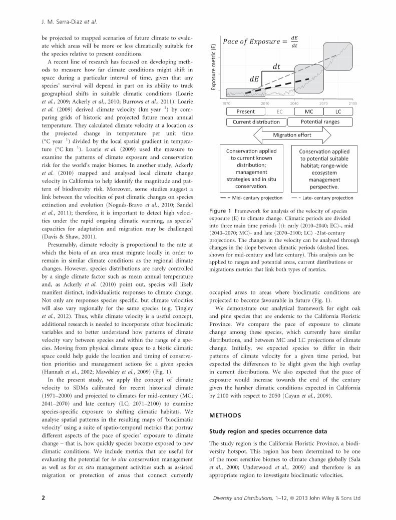
1970 2010 2040 2070 2100

Present EC MC LC

Poten al rangesCurrent distribu on

Expo

sure

met

ric (E

)

Conserva on applied to poten al suitable habitat; range-wide

ecosystemmanagement perspec ve.

Conserva on applied to current known

distribu on; management

strategies and in situ conserva on.

Migra on effort

Mid- century projec on Late- century projec on

Figure 1 Framework for analysis of the velocity of species

exposure (E) to climate change. Climatic periods are divided

into three main time periods (t): early (2010–2040; EC)-, mid

(2040–2070; MC)- and late (2070–2100; LC) -21st-century

projections. The changes in the velocity can be analysed through

changes in the slope between climatic periods (dashed lines,

shown for mid-century and late century). This analysis can be

applied to ranges and potential areas, current distributions or

migrations metrics that link both types of metrics.

2 Diversity and Distributions, 1–12, ª 2013 John Wiley & Sons Ltd

J. M. Serra-Diaz et al.

Our target species encompass eight species of oak and pine

trees endemic to the California Floristic Province: Pinus

balfouriana [Grev.&Balf.], Pinus coulteri [D.Don], Pinus mu-

ricata [D.Don.], Pinus sabiniana [D.Don], Quercus douglasii

[Hook.&Arn.], Quercus engelmannii [Greene], Quercus lobata

[Nee] and Quercus wislizeni [A.DC.]. These endemic species

are dominant and widespread in the landscape, and there-

fore, they all play important roles in providing ecosystem

services (carbon storage, wood production, wildlife habitat,

etc.). Additionally, oaks woodlands are especially subject to

conservation and sustainable development by the state (the

California Legislature passed the Oak Woodland Conserva-

tion Act in 2001).

Species occurrence data were extracted from 42 existing

vegetation inventories (compiled by Hannah et al., 2008)

comprising probabilistic and purposive sample designs. Only

records from presence/absence vegetation surveys were used

[P. balfouriana (n = 217), P. coulteri (n = 323), P. muricata

(n = 65), P. sabiniana (n = 2372), Q. douglasii (n = 2422),

Q. engelmannii (n = 36), Q. lobata (n = 699) and Q. wislizeni

(n = 2763)].

Environmental data

Current climatic variables were obtained from a statistical

downscaling (Flint & Flint, 2012) of the PRISM database

(PRISM Climate Group, Oregon State University, available

at: http://prism.oregonstate.edu) from 800-m to 270-m spa-

tial resolution, including total annual precipitation, mean

annual temperature, precipitation of the driest month, max-

imum temperature of the warmest month and minimum

temperature of the coldest month. Although different

species may be limited more or less by different subsets of

these variables, we included all variables in the models to

ensure maximum comparability among species and at the

same time depict both averaged and extreme climatic

ranges.

Species distribution models and climate change

projections

Using averaged climate data for the period 1971–2000, we

estimated eight different SDMs for each species within the

BIOMOD platform (Thuiller et al., 2009; see Appendix S1 in

Supporting Information for model descriptions) in order to

obtain a robust measure of species climatic suitability based

on model consensus (Ara�ujo & New, 2007). Model calibra-

tion was undertaken with 70% of the presence/absence

observations, and the remaining 30% were used for valida-

tion. We randomly selected 5000 absences from the many

absences available for each species in the presence/absence

dataset, allowing for a large number of absences covering the

environmental space (Barbet-Massin et al., 2012). In addi-

tion, each model was run twice using different random sam-

ples of absence to address potential sample bias in absences

(Elith et al., 2010).

In order to discriminate suitable from unsuitable areas, a

threshold was applied to the continuous climatic suitability

measure predicted by each SDM. We selected the threshold

that maximized the true skill statistic (TSS) metric because

this metric is unaffected by prevalence (Allouche et al.,

2006). Current and future suitable areas were then identified

based on the agreement of at least five models in considering

an area suitable after binary conversion using maximum TSS

(committee averaging; see Gallien et al., 2012 for details). A

continuous consensus climatic suitability was then obtained

for each grid cell by averaging the probabilities from those

models agreeing with the consensus of suitable area.

Although threshold choice may affect our results, major

sources of uncertainty come from the choice of the statistical

technique (Nenz�en & Ara�ujo, 2011). In our case, we have

chosen an optimization threshold that balances correct

prediction of presences and absences.

Habitat suitability dynamics were estimated based on dif-

ferences between models’ consensus projection for current

climate and for future projected climate under the A2 emis-

sions scenario using two global circulation models (GCMs):

Geophysical Fluid Dynamics Laboratory (GFDL) and Parallel

Climate Model (PCM). These GCMs were selected for cli-

mate change assessment in California because of their ability

to reproduce historic climate patterns accurately (Cayan

et al., 2008). This combination of GCMs and scenario repre-

sents a ‘strong change’ scenario of a much warmer and drier

California used by the California Climate Change Center for

impact analysis (Cayan et al., 2009) and to derive informed

conservation policies. In order to assess potential differences

in species exposure over time, two climate change periods

were set: mid-21st-century (averaged climate 2041–2070;

MC) and the late 21st century (averaged climate 2071–2100;

LC). We did not perform early-century projections (2011–

2040; Fig. 1) to avoid issues of temporal autocorrelation with

historic climate.

Bioclimatic velocity estimation

We computed the species’ bioclimatic velocity of climate

change using the same procedure as in Loarie et al. (2009),

but applied to each species’ suitability maps rather than to a

single climate variable. We divided the temporal gradient

(e.g. magnitude of change over time) of climate suitability by

the spatial gradient (e.g. magnitude of change over space) in

suitability for the period under analysis. The temporal gradi-

ent is computed as the difference in consensus probabilities

between present and future projection per unit of time

(years) for each map cell: 70 years for MC projection and

100 years for LC projection. Spatial gradients are computed

for each map cell as the slope of probabilities using the max-

imum average technique (Burrough & McDonnell, 1998) in

a 9-cell kernel (8-neighbour rule). To avoid infinite veloci-

ties, we excluded flat spatial gradients. The result is a velocity

measure of the changes in climatic suitability of each species

within its potential climatic range. Bioclimatic velocity has a

Diversity and Distributions, 1–12, ª 2013 John Wiley & Sons Ltd 3

Species exposure velocity to climate change risk

sign determined by the loss (negative) or gain (positive) in

climatic suitability over time. However, the essence of the

estimate is the same as for climate velocity sensu Loarie et al.

(2009): combine local variation in suitable conditions

(rather than in a given climatic variable) with the temporal

gradient of change in suitable conditions. Bioclimatic velocity

of each species was calculated as the average between the

velocities based on each of the two GCMs for each period

analysed.

Dynamic exposure metrics

In order to evaluate how patterns of changing habitat suit-

ability may affect different conservation strategies, we calcu-

lated several metrics that focus on the range level (referring

to climatically suitable areas) and the population level (refer-

ring to current distributions of species within plots) (Fig. 1).

Metrics are used to describe the pace of exposure to climate

change and are based on bioclimatic velocity, potentially

suitable areas and habitat suitability. Range-level metrics pro-

vide information most relevant to developing conservation

strategies that address broad patterns of change in climate

suitability, including potential new areas for colonization

(whether assisted or not), whereas the population-level met-

rics inform more local management strategies focused on

species’ adaptation and in situ conservation (see Appendix

S2 in Supporting Information for detailed description of the

metrics). The estimates for each metric were derived from

averaging values based on both GCMs in the period of analy-

sis. In the case of high deviation from centrality, median

values were used.

At the range level, five metrics were calculated:

(1) rate of species range change (SRC), which measures

differences in potential suitable area gained and potential

suitable area loss (Thuiller et al., 2005) per unit of time (year)

and is related to exposure to extinction due to rapid habitat

loss; (2) rate of range exposure to migration (REM), calcu-

lated as the difference in suitable habitat area between full

and null dispersal assumptions (Svenning & Skov, 2004; Ara-

�ujo & New, 2007) divided by the time lapse between the cur-

rent and targeted period, which emphasizes the importance

of migration processes in lowering exposure; (3) range change

velocity (RCV), which identifies potential impediments to

tracking climate change at the edges of ranges, calculated as

the net balance between trailing edge and leading edge biocli-

matic velocity. Both trailing (suitable ? unsuitable) and

leading edges (unsuitable ? suitable) were identified on a

cell-by-cell basis using the consensus of SDMs on changes in

suitability; (4) range spatial fragmentation (RSF), calculated

as the number of discrete habitat patches gained or lost

(McGarigal, 2013), and (5) range spatial aggregation (RSA),

calculated as the percentage gain or loss of total suitable habi-

tat occupied by the largest patch (McGarigal, 2013). These

landscape structure metrics assess the spatial configuration of

potential suitable habitat, which is related to population

persistence (Opdam & Wascher, 2004).

To assess population-level exposure of current woodlands

(e.g. the eight tree species are found in forests, open wood-

lands or savannas), we defined three metrics:

(1) Population migration exposure (PME), which mea-

sures the mean distance of plots containing the target spe-

cies to projected future climatically suitable area using a

least cost-distance route based on suitability measures. Skov

& Svenning (2004) used a similar approach based on tree

cover to assess potential migration routes for European

herbs, and Wang et al. (2008) found a significant relation-

ship between gene flow and a suitability resistance measure;

(2) population climate-site exposure (PCE), calculated as

the percentage of species plot locations switching from suit-

able to unsuitable conditions based on the set threshold of

habitat suitability, divided by the time lapse between projec-

tions. Although this measure has been used as a surrogate

for extinction risk (Thomas et al., 2004), we have adopted

it as a measure of woodland exposure risk to new climatic

conditions; and (3) population climatic velocity (PCV), the

mean bioclimatic velocity of species plots decreasing in suit-

ability, calculated by overlaying woodland plots with the

bioclimatic velocity grid computed using the methods

described above.

We further performed hierarchical clustering in order to

investigate the degree of similarity among species and

projection times (MC and LC). First, we built a dissimilarity

matrix using Mahalanobis multivariate distance and using

the values for each metric as input variables. Subsequently,

we calculated the clustering dendrogram using Ward’s

method of minimum variance among clusters.

RESULTS

Species distribution models accuracy

Species distribution models were able to reproduce current

distributions with acceptable accuracy in discrimination

capacity based on TSS (see Table S1 in Supporting Infor-

mation). However, the accuracy varied between species (see

Fig. S1 in Supporting Information), ranging from 0.65 TSS

(Q. lobata and P. muricata) to 0.89 and 0.91 TSS (P. bal-

fouriana and Quercus sabiniana, averaged values across

models). For most species analysed, the range of accuracy

values across models varied between 0.10 and 0.15. How-

ever, P. muricata exhibited a large range due to the poor fit

of some models (flexible discriminant analysis and multiple

adaptive regression splines). The difference between TSS val-

ues was greater across species than across models (see

Fig. S1).

Species bioclimatic velocity

Bioclimatic velocities vary greatly within each species

potential range and in the climate change periods analysed

(Fig. 2, Table 1). Mean values of bioclimatic velocity range

between 0.11 and 0.32 km year�1 depending on the species

4 Diversity and Distributions, 1–12, ª 2013 John Wiley & Sons Ltd

J. M. Serra-Diaz et al.

and period (Table 1). The spatial distribution of

bioclimatic velocities for these California foothill and

mountain pines and oaks exhibits high velocities leading to

climatic unsuitability located in and around the large, flat

Great Central Valley, whereas high velocities of increasing

climatic suitability tend to concentrate in northern

mountain ranges, although this pattern varied by species.

Nevertheless, patterns of similarity emerge between species

with overlapping ranges. For instance, P. sabiniana and

Q. douglasii show a similar pattern of range dynamics and

velocity; they increase at a higher rate in the northern

mountains.

Predicted velocities are different for each period of analy-

sis. Mean velocities suggest that most species analysed will

experience higher bioclimatic velocities towards the end of

the 21st century (LC), with an increase of 0.05 km year�1 on

average with respect to the bioclimatic velocities of the MC

(Table 1). However, two species (P. coulteri and Q. lobata)

show the opposite pattern (Table 1). Correlations between

periods for each species are relatively high (0.67 on average,

Table 1).

The pace of climate change exposure for ranges

Species ranges (the extent of climatically suitable habitats)

are predicted to shrink except for P. balfouriana in MC

(Fig. 3a; SRC). Half of the species (4) have higher rates of

loss in MC, and the other half in LC (Table 2). In general,

differences in SRC between the two GCMs are larger for the

MC projections than for the LC projections (Fig. 3a;

Table 2; see also Appendix S3 in Supporting Information for

range change maps by GCMs). REM is predicted to be

higher in LC for the five of eight species analysed (Fig. 3b;

Table 2). Likewise, the range of values of this metric

Table 1 Global circulation model-averaged bioclimatic velocities (km year�1) for species and time periods analysed. Values between

brackets indicate 5% and 95% percentiles. Difference and Kendall correlation are between the climate periods.

Mean bioclimatic velocity (km year�1) [5–95

percentiles]

Difference

Kendall

correlationMid-century Late century

Pinus balfouriana 0.21 [0.01–0.88] 0.28 [0.01–1.14] 0.07 0.64

Pinus coulteri 0.13 [0.01–0.42] 0.11 [0.01–0.35] �0.02 0.85

Pinus muricata 0.14 [0.00–0.57] 0.18 [0.01–0.70] 0.03 0.65

Pinus sabiniana 0.17 [0.01–0.66] 0.24 [0.01–1.01] 0.07 0.69

Quercus douglasii 0.28 [0.01–1.23] 0.30 [0.01–1.32] 0.02 0.69

Quercus engelmannii 0.21 [0.02–0.99] 0.32 [0.01–1.77] 0.11 0.62

Quercus lobata 0.29 [0.01–1.16] 0.28 [0.01–1.09] �0.02 0.69

Quercus wislizeni 0.11 [0.00–0.40] 0.13 [0.01–0.50] 0.03 0.57

Averages 0.19 0.23 0.05 0.67

Figure 2 Averaged bioclimatic velocity

of climate change for different California

endemic tree species within their

potential range, based on two global

circulation models (GCMs) and eight

species distribution models. (a)

Bioclimatic velocity map for the period

present (1971–2000) to late 21st century

(2071–2100). Inset in Fig. 1 shows how

different velocities may occur within

relatively short geographical distances.

PIBA = Pinus balfouriana, PICO = Pinus

coulteri, PIMU = Pinus muricata,

PISA = Pinus sabiniana,

QUEN = Quercus engelmannii,

QUDO = Quercus douglasii,

QULO = Quercus lobata,

QUWI = Quercus wislizeni.

Diversity and Distributions, 1–12, ª 2013 John Wiley & Sons Ltd 5

Species exposure velocity to climate change risk

increases in LC due to the differences in GCM projections

(Table 2).

Bioclimatic velocity is generally higher in the leading edge

than in the trailing edge (positive values in Fig. 3c), but the

magnitude is species- and period-dependent (Fig. 3c). This

pattern is reinforced in LC for six of eight species (Table 2),

the exceptions being Q. lobata and Q. wislizeni. P. muricata

and P. coulteri do not change notably between periods

(Fig. 3c). The range of values of the metric (RCV) increases

from MC to LC for seven of eight species (Table 2), and con-

flicting trends may appear under single GCM scenarios (see

Appendix S4 in Supporting Information for GCM bioclimatic

velocities). It is noteworthy that negative velocities are found

within stable ranges (areas preserving climatic suitability), pro-

viding a signal of increasing exposure in such areas (see Fig. S2

in Supporting Information for velocities in stable ranges).

Landscape structure metrics (RSF and RSA) depict a general

pattern (for five of eight of the species) of spatial erosion of

the largest suitable patch combined with the loss of other small

suitable patches (Fig. 3d,e). This pattern tends to be exacer-

bated in LC by decreased number of patches (three-quarters of

the species) and increased aggregation (three-quarters of the

species) (Table 2). There are exceptions to this pattern

(Q. engelmannii and P. sabiniana) that also depend on the

GCM projection (see bar ranges in Fig. 3d,e).

The pace of climate change exposure for current

woodlands

Woodlands are predicted to experience decreasing climatic

suitability with climate change; the majority of plots experi-

ence negative bioclimatic velocities (PCV, Fig. 4a) and posi-

tive rates of suitability loss (PCS, Fig. 4b). However, a few

plots are projected to increase its climatic suitability (see bar

depicting range of values). There is no general trend to

whether these metrics increase (half of the species) or

decrease (half of the species) depending on the temporal

projection (MC or LC; Table 2).

The projected rate of isolation of current woodlands from

potential suitable areas (measured by climate paths), or pop-

ulation migration exposure (PME, Fig. 4c), varies widely

among species and time projections: from ca. 6 m year�1 to

871 m year�1. For most species, this rate of climatic isolation

doubles from MC to LC (seven of eight of the species;

Table 2). The presence of many outliers indicates disjunct

populations (Fig. 3c). This is especially the case for P. bal-

fouriana with a few southern populations predicted to

become very isolated in LC (Fig. 4c).

Varying exposure rates

The rates of exposure (averaging across metrics) increase

towards the LC for 4.75 of 8 species on average (Table 2),

and the uncertainty in the metrics derived from using differ-

ent GCMs decreases towards LC for 4.5 of 8 species on aver-

age (Table 2). Exposure rates are more sensitive to species

than temporal projections, with average standard deviations

of the metrics among species (7.3) being greater than across

periods (3.5), and this pattern remains constant for all

metrics analysed (Table 2).

Three species (P. balfouriana, P. muricata and Q. wislizeni)

depict very similar exposure rates between periods for all

metrics, while exposure rate is dramatically increased or

decreased in one or more dimensions for other species (e.g.

Q. engelmannii, P. coulteri; Fig. 5a). Similarities between spe-

cies and periods suggest processes (e.g. dispersal, migration)

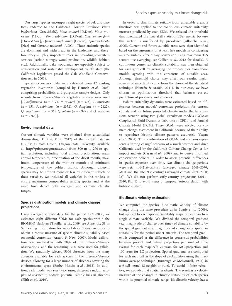
Table 2 Comparison of metrics across species and projections

Projection trends Projection breadth trends

VariabilityIncrease Decrease Increase Decrease

Small Large Total Small Large Total Small Large Total Small Large Total SD periods SD species

SRC 3 1 4 4 0 4 1 0 1 7 0 7 0.22 0.50

REM 5 0 5 3 0 3 3 2 5 3 0 3 0.13 0.26

RCV 4 2 6 2 0 2 4 3 7 1 0 1 0.04 0.12

RSA 5 1 6 1 1 2 1 3 4 4 0 4 0.29 0.49

RSF 2 0 2 2 4 6 1 1 2 6 0 6 0.21 0.72

PCV 4 0 4 4 0 4 4 0 4 4 0 4 0.00 0.02

PCS 4 0 4 4 0 4 0 0 0 8 0 8 0.15 0.29

PME 0 7 7 0 1 1 0 5 5 3 0 3 27.13 55.93

Average 3.375 1.375 4.75 2.5 0.75 3.25 1.75 1.75 3.5 4.5 0 4.5 3.5 7.3

Projection trends indicate the number of the eight species with a predicted increase or decrease for a metric between mid-21st-century projection

[mid-century (MC)] and late-21st-century projection [late century (LC)]. Projection breadth trends indicate the number of species with an

increase or decrease in the range of values from MC to LC according to the different global circulation models used. Large increases/decreases

indicate that the magnitude of change in the metric is greater than the value of the metric in the MC, while small is less than that value. Variabil-

ity indicates the standard deviation (SD) of the metric across species and periods. Metrics: species range change (SRC), range exposure to migra-

tion (REM), range change velocity (RCV), range spatial aggregation (RSA), range spatial fragmentation (RSF); population climatic velocity

(PCV), population change in suitability (PCS) and population migration effort (PME). See Table S2 for individual metrics results.

6 Diversity and Distributions, 1–12, ª 2013 John Wiley & Sons Ltd

J. M. Serra-Diaz et al.

that may play key roles in exposure for each time frame

analysed (Fig. 5b).

DISCUSSION

Measuring the pace of changing climatically suitable

conditions: bioclimatic velocity

The bioclimatic velocity measurement proposed in this study

extends the concept of climate velocity to depict species-specific

exposure to climate change. That translation from physical

attributes (e.g. temperature, precipitation) to an integrated

measurement of climatic suitability has the advantage of

depicting how fast suitable conditions appear or disappear for

a given species and period.

The bioclimatic velocity maps show congruent patterns

using analogous metrics to climate velocities presented in

Loarie et al. (2009), Ackerly et al. (2010) and Dobrowski

et al. (2013) for temperature, precipitation and actual evapo-

transpiration in California. Flat areas exhibit higher velocities

than mountainous areas where varying climatic conditions in

space tend to be large. This steep spatial gradient thus

reduces velocity estimates in mountainous areas.

Bioclimatic velocities are slightly lower than the climate

velocity presented for a larger extent by Ackerly et al. (2010):

0.21 km year�1 for bioclimatic velocity (average of species

and periods) compared to 0.24 km year�1 for mean temper-

ature velocity. Also, the range of our 5–95 percentiles is

generally lower than those in Ackerly et al. (2010): they esti-

mated 0.03–4.89 km year�1 for temperature velocity and

0.01–0.92 km year�1 for precipitation velocity in the drier

scenario (GFDL) and 0.01–0.46 km year�1 for precipitation

velocity in the wetter scenario (PCM), whereas bioclimatic

velocity in our study ranged from 0.01 to 0.89 km year�1.

Some discrepancies would be expected because the use of

SDMs to transform combinations of raw climate variables

into an associated measure of habitat suitability may affect

the spatial variation of suitability relative to that of climate

alone. Ultimately, the spatial gradient affects the magnitude

of the velocity being estimated. Therefore, it is not surprising

that bioclimatic velocities could be different than climate

velocities. In our study, we used an ensemble of SDMs to

(a) (b)

(c) (d)

(e)

Figure 3 The pace of climate change exposure in range-level metrics. Mid-century projections are in light grey, and late-21st-century

projections in black. Hollow bars indicate the range of the two global circulation models (GCMs) predictions, and middle bar indicates

average. (a) Species range change (SRC); (b) range exposure to movement (REM): time rates between full versus null dispersal in their

ranges; (c) range change velocity (RCV): differences between velocities of leading edge and trailing edge; (d) range spatial aggregation

(RSA): percentage of area change of the species’ largest suitable habitat patch per unit of time; (e) range spatial fragmentation (RSF):

percentage of patch abundance increase/decrease per unit of time. Species abbreviations are defined in Fig. 2 caption. See Table S2

(Supporting Information) for individual metrics results.

Diversity and Distributions, 1–12, ª 2013 John Wiley & Sons Ltd 7

Species exposure velocity to climate change risk

address the inherent uncertainty of using different statistical

approaches (Ara�ujo & New, 2007). However, further research

on bioclimatic velocity could estimate the sensitivity of

bioclimatic velocity to the SDM technique used.

Spatial resolution is another source of variation between

climate and bioclimatic velocity estimates. Dobrowski et al.

(2013) found that coarser resolutions increase estimates of

climate velocity, and therefore, it is not surprising that

bioclimatic velocities presented here and based on 270-m

resolution data are lower than climate velocities found by

other authors who used coarser climate grids (e.g. Loarie

et al., 2009; Burrows et al., 2011; Dobrowski et al., 2013).

Individualistic paces of exposure to climate change

We illustrate that the velocity of species’ exposure to climate

change varies depending on the species, within each species

range and period under analysis. These results reinforce the

importance of transforming from physical climate space to

biotic climate space (suitability), as differences are clear even

in the case of similarly distributed species and using the

same predictor variables. Broadly, the results presented in

this study are generally consistent with other projections of

range shrinkage, fragmentation and overall loss of climatic

suitability for plant species in the study region (Loarie et al.,

2008; Franklin et al., 2013), but here we illustrate the inher-

ent variation in the rates of change of metrics that are indi-

ces of exposure risk and potential woodland dynamics.

The taxonomic and temporal variation found in this study

largely supports the conclusions raised by several modelling

and observational studies, which have also identified diverse

patterns of range dynamics at the specific level. For instance,

in our case, the velocity of gaining environmental suitability

in potential leading edges of ranges is generally higher than

the suitability loss in trailing edges. Accordingly, some stud-

ies have shown that the leading edge of the range may

become occupied at higher rates than the trailing edge is

vacated (Chen et al., 2011 showed for Lepidoptera). How-

ever, other studies have suggested that most tree species may

not be able to keep pace with expansion of suitable habitat

at the leading edge (Foden et al., 2007; Murphy et al., 2010),

although such response may be species specific (Zhu et al.,

2012). In these cases, accumulation of extinction debt may

occur at trailing edges especially for long-lived organism such

as trees (Kuussaari et al., 2009). These effects could ulti-

mately result in shrinking distributions. Our study empha-

sizes a common trend of range reduction (range metrics:

SRC, RSF, RSA) and an overall increased exposure of popu-

lations (plot metrics: PCS, PCV), although at different

paces depending on the species and differentially across

populations.

All in all, temporal variations in exposure generally

support the idea of an acceleration of exposure by the end of

the century, coinciding with major predicted changes in tem-

perature and precipitation (Cayan et al., 2009). However,

this support is not strong (five of the eight species showed

(a)

(b)

(c)

Figure 4 The pace of climate change exposure in plot-level metrics (current distribution). Mid-century projections are in light grey,

and late-21st-century projections in black. Hollow bars indicate the range of the two global circulation models (GCMs) predictions, and

middle bar indicates average. Boxplots indicate the distribution of values in current plots. (a) population change in bioclimatic velocity

(PCV): velocity of bioclimatic exposure in species plots; (b) population change in suitability (PCS): percentage of plots becoming

unsuitable per unit of time; (c) population migration exposure (PME): cost-distance to the nearest suitable patch. Inset represents zoom

to the interquartile distribution of values. Species abbreviations are defined in Fig. 2 caption. See Table S2 for individual metrics results.

8 Diversity and Distributions, 1–12, ª 2013 John Wiley & Sons Ltd

J. M. Serra-Diaz et al.

increasing bioclimatic velocity estimates) and especially low

in the case of current population-level metrics (PCV, PCS).

These results emphasize that adaptive capacity may be crucial

for some species, as changing suitability will challenge some

species faster than others and may occur sooner than later.

Challenges ahead: climate variability, extremes and

microclimates

The metrics used in this study constitute a first approxima-

tion of the velocity of species exposure of climate change.

However, it is noteworthy that the application of SDMs to

assess exposure in dynamic environments may be further

limited by the static nature of the models and the scale of

analysis (Franklin, 2010b), in addition to other widely

discussed limitations (see Fitzpatrick & Hargrove, 2009;

Franklin, 2010a; Keenan et al., 2011; Schwartz, 2012).

In previous studies of the velocity of climate change, tem-

poral gradients were estimated with a linear regression over

time. Therefore, climate variability and extremes are indirectly

taken into account. For instance, Dobrowski et al. (2013)

used a yearly interpolation of climate variables to calculate

velocity of climate, which further provided a measure of

significance for velocity, after correcting for temporal auto-

correlation. In contrast, SDMs with their quasi-equilibrium

assumption and reliance on species distribution data for

adult or mixed-age individuals are usually calibrated from

and projected to climatic scenarios (30-year averages define

climate); therefore, these models are not suitable for

providing velocity estimates at finer temporal resolutions.

In our case, an SDM implementation using climate vari-

ables at finer temporal resolution would face several chal-

lenges. First, the role of climate variability and extremes in

shaping plant species distribution is poorly understood. On

(a)

(b)

Figure 5 Differences in the pace of

climate change exposure among species

and periods across all metrics: (a) extent

of exposure rates across species for mid-

21st-century projections [mid-century

(MC), grey], late-21st-century projections

[late century (LC) dark grey] and (b)

dendrogram of similarity among species-

projection rates. Dark grey cross and

light grey cross indicate LC and MC,

respectively. Black stars in the

dendrogram indicate high similarity

among the two time periods: the

majority of species below the branch

contain both LC and MC projections of

the same species. Species abbreviations

are defined in Fig. 2 caption.

Diversity and Distributions, 1–12, ª 2013 John Wiley & Sons Ltd 9

Species exposure velocity to climate change risk

the one hand, extreme events are shown to increase model

accuracy (albeit weakly) for species distributions (Zimmer-

mann et al., 2009), but Larcher & Mair (1969) showed that

temperature extremes alone could not explain range limits in

Mediterranean oaks. Altogether, it may be difficult to disen-

tangle both roles using correlative approaches, as means and

extremes tend to be highly correlated.

Second, weather variability differentially affects tree life

stages, which may confound the response variable of SDMs.

That is, seedling survival and germination may be strongly

affected by this variability (Thompson et al., 2012; Nabel

et al., 2013), but advanced life stages of trees may not. Cru-

cially, this issue affects range migration estimates (Early &

Sax, 2011; Bennie et al., 2013), but may not be meaningful

for plot-level metrics of suitability (e.g. conditions of the

current distribution of adult trees) as adults are far more

resilient (Lloret et al., 2012). Interestingly, SDMs can be fit

using weather variables together with climate means for vag-

ile organisms (see Reside et al., 2010; Bateman et al., 2012;

and VanDerWal et al., 2013). Indeed, such an approach is

appropriate for mobile organisms or those with a short life

cycle because their distribution is able to reflect variation in

climate at finer temporal resolution. Third, it may be conten-

tious to use GCM projections of climate variability and

extremes (in contrast to observations of historical variability)

to provide a framework for evaluating significant trends.

Unlike averaged values, finer temporal and spatial resolutions

and extreme events still report considerable uncertainty, even

with the recent advancements of new generation of GCM

(Sillmann et al., 2013).

The role of microclimates (and thus spatial resolution of

the analysis) can be very important in buffering future

temperature and precipitation changes (Bennie et al., 2013;

Lenoir et al., 2013). Exposure estimates should reflect such

variations in space. In our study region, analogous spatial

resolution sensitivity analysis has also been performed for

SDMs. Franklin et al. (2013) showed that there are large

differences (both omission and commission) between suitable

habitats predicted from coarse- versus fine-scale climate

grids, concluding that the 270-m resolution used in the pres-

ent study is adequate to capture some fine-scale effects of

topoclimate on species distributions.

CONCLUSIONS

Transformation of physical climate space to a more biologi-

cally meaningful climate space can support species-specific

conservation measures. Our results emphasize that climate

velocities can be species specific but may vary within its

range and among periods. Areas of low bioclimatic velocity

may be high-priority targets for in situ conservation (land

conservation, woodland reserves) for a given species and

time period, while areas of high velocity increases in habitat

suitability may be appropriate targets for, for example,

climate change adaptation strategies such as managed reloca-

tion. Areas of rapidly decreasing suitability, especially for

species whose plot metrics also suggest increasing exposure,

would indicate to managers where woodland health may be

expected to decline and where community changes may be

anticipated. Limitations still constrain the use of SDMs to

make dynamic predictions, however, and careful calibration

and sufficient ecological data are necessary for meaningful

habitat suitability estimates.

ACKNOWLEDGEMENTS

J.M.S.D. acknowledge the support from UAB mobility pro-

gramme and the research group GRUMETS (2009SGR1511).

This research was supported in part by grants from the U.S.

Department of Energy (DE-FC02-06ER64159) and U.S.

National Science Foundation (BCS-0824708, EF-1065826 and

EFG-1065864). The work represents the findings of the

authors and does not reflect the opinion of the sponsors. We

are grateful to A. and L. Flint for providing access to down-

scaled climate data. We would especially thank B. Beltr�an,

J. Ripplinger, J. Ramos, M. Naciff, L. Reichmann and L.

Ghardi for enlightening discussions.

REFERENCES

Ackerly, D., Loarie, S., Cornwell, W., Weiss, S., Hamilton,

H., Branciforte, R. & Kraft, N. (2010) The geography of

climate change: implications for conservation biogeogra-

phy. Diversity and Distributions, 16, 476–487.

Allouche, O., Tsoar, A. & Kadmon, R. (2006) Assessing the

accuracy of species distribution models: prevalence, kappa

and the true skill statistic (TSS). Journal of Applied Ecology,

43, 1223–1232.

Ara�ujo, M.B. & New, M. (2007) Ensemble forecasting of spe-

cies distributions. Trends in Ecology and Evolution, 22,

42–47.

Ara�ujo, M.B., Alagador, D., Cabeza, M., Nogu�es-Bravo, D. &

Thuiller, W. (2011) Climate change threatens European

conservation areas. Ecology Letters, 14, 484–492.

Barbet-Massin, M., Jiguet, F., Albert, C.H. & Thuiller, W.

(2012) Selecting pseudo-absences for species distribution

models: how, where and how many? Methods in Ecology

and Evolution, 3, 327–338.

Bateman, B.L., VanDerWal, J. & Johnson, C.N. (2012) Nice

weather for bettongs: using weather events, not climate

means, in species distribution models. Ecography, 35,

306–314.

Bennie, J., Hodgson, J.A., Lawson, C.R., Holloway, C.T.R.,

Roy, D.B., Brereton, T., Thomas, C.D. & Wilson, R.J.

(2013) Range expansion through fragmented landscapes

under a variable climate. Ecology Letters, 16, 921–929.

Burrough, P.A. & McDonnell, R.A. (1998) Principles of GIS.

Oxford University Press, Oxford.

Burrows, M.T., Schoeman, D.S., Buckley, L.B., Moore, P.,

Poloczanska, E.S., Brander, K.M., Brown, C., Bruno, J.F.,

Duarte, C.M. & Halpern, B.S. (2011) The pace of shifting

10 Diversity and Distributions, 1–12, ª 2013 John Wiley & Sons Ltd

J. M. Serra-Diaz et al.

climate in marine and terrestrial ecosystems. Science, 334,

652–655.

Cayan, D.R., Maurer, E.P., Dettinger, M.D., Tyree, M. &

Hayhoe, K. (2008) Climate change scenarios for the Cali-

fornia region. Climatic Change, 87, 21–42.

Cayan, D.R., Tyree, M., Dettinger, M.D., Hidalgo, H., Das,

T., Maurer, E., Bromirski, P., Graham, N. & Flick, R.

(2009) Climate change scenarios and sea level rise estimates

for the California 2009 Climate Change scenario Assess-

ment. California Energy Commission-California Ocean

Protection Council-California Environmental Protection

Agency.

Chen, I., Hill, J.K., Shiu, H., Holloway, J.D., Benedick, S.,

Chey, V.K., Barlow, H.S. & Thomas, C.D. (2011) Asym-

metric boundary shifts of tropical montane Lepidoptera

over four decades of climate warming. Global Ecology and

Biogeography, 20, 34–45.

Davis, M. & Shaw, R. (2001) Range shifts and adaptive

responses to Quaternary climate change. Science, 292,

673–679.

Dawson, T.P., Jackson, S.T., House, J.I., Prentice, I.C. &

Mace, G.M. (2011) Beyond predictions: biodiversity con-

servation in a changing climate. Science, 332, 53–58.

Dobrowski, S.Z., Abatzoglou, J., Swanson, A.K., Greenberg,

J.A., Mynsberge, A.R., Holden, Z.A. & Schwartz, M.K.

(2013) The climate velocity of the contiguous United States

during the 20th century. Global Change Biology, 19, 241–251.

Early, R. & Sax, D.F. (2011) Analysis of climate paths reveals

potential limitations on species range shifts. Ecology Letters,

14, 1125–1133.

Elith, J., Kearney, M. & Phillips, S. (2010) The art of model-

ling range-shifting species. Methods in Ecology and Evolu-

tion, 1, 330–342.

Fitzpatrick, M. & Hargrove, W. (2009) The projection of

species distribution models and the problem of non-analog

climate. Biodiversity and Conservation, 18, 2255–2261.

Flint, L.E. & Flint, A.L. (2012) Downscaling future climatic

scenarios to fine scales for hydrologic and ecological

modeling and analysis. Ecological Processes, 1, 2.

Foden, W., Midgley, G.F., Hughes, G., Bond, W.J., Thuiller,

W., Hoffman, M.T., Kaleme, P., Underhill, L.G., Rebelo, A.

& Hannah, L. (2007) A changing climate is eroding the

geographical range of the Namib Desert tree Aloe through

population declines and dispersal lags. Diversity and Distri-

butions, 13, 645–653.

Franklin, J. (2010a) Mapping species distributions: spatial

inference and prediction. Cambridge University Press,

Cambridge.

Franklin, J. (2010b) Moving beyond static species distribu-

tion models in support of conservation biogeography.

Diversity and Distributions, 16, 321–330.

Franklin, J., Davis, F.W., Ikegami, M., Syphard, A.D., Flint,

L.E., Flint, A.L. & Hannah, L. (2013) Modeling plant spe-

cies distributions under future climates: how fine scale do

climate projections need to be? Global Change Biology, 19,

473–483.

Gallien, L., Douzet, R., Pratte, S., Zimmermann, N.E. & Thu-

iller, W. (2012) Invasive species distribution models – how

violating the equilibrium assumption can create new

insights. Global Ecology and Biogeography, 21, 1126–1136.

Hannah, L., Midgley, G.F. & Millar, D. (2002) Climate

change-integrated conservation strategies. Global Ecology

and Biogeography, 11, 485–495.

Hannah, L., Midgley, G., Davies, I., Davis, F., Ries, L., Thuiller,

W., Thorne, J., Seo, C., Stoms, D. & Snider, N. (2008) Bio-

Move – Improvement and Parameterization of a Hybrid

Model for the Assessment of Climate Change Impacts on the

Vegetation of California. CEC-500-02-004, California Energy

Commission, Public Interest Energy Research Program.

Keenan, T., Serra-Diaz, J.M., Lloret, F., Ninyerola, M. & Sabat�e,

S. (2011) Predicting the future of forests in the Mediterra-

nean under climate change, with niche- and process-based

models: CO2 matters!. Global Change Biology, 17, 565–579.Kuussaari, M., Bommarco, R., Heikkinen, R.K., Helm, A.,

Krauss, J., Lindborg, R., €Ockinger, E., P€artel, M., Pino, J.,

Rod�a, F., Stefanescu, C., Teder, T., Zobel, M. & Steffan-Dew-

enter, I. (2009) Extinction debt: a challenge for biodiversity

conservation. Trends in Ecology and Evolution, 24, 564–571.

Larcher, W. & Mair, B. (1969) The temperature resistance as

ecophysiological trait: 1. Quercus ilex and other Mediterra-

nean oak species (Translated from German). Oecologia

Plantarum, 4, 347–376.

Lenoir, J., Graae, B.J., Aarrestad, P.A. et al. (2013) Local

temperatures inferred from plant communities suggest

strong spatial buffering of climate warming across North-

ern Europe. Global Change Biology, 19, 1470–1481.

Lloret, F., Escudero, A., Iriondo, J.M., Mart�ınez-Vilalta, J. &

Valladares, F. (2012) Extreme climatic events and vegeta-

tion: the role of stabilizing processes. Global Change Biol-

ogy, 18, 797–805.

Loarie, S.R., Carter, B.E., Hayhoe, K., McMahon, S., Moe, R.,

Knight, C.A. & Ackerly, D.D. (2008) Climate change and the

future of California’s endemic flora. PLoS One, 3, e2502.

Loarie, S.R., Duffy, P.B., Hamilton, H., Asner, G.P., Field,

C.B. & Ackerly, D.D. (2009) The velocity of climate

change. Nature, 462, 1052–1055.

Mawdsley, J.R., O’Malley, R. & Ojima, D.S. (2009) A review

of climate-change adaptation strategies for wildlife manage-

ment and biodiversity conservation. Conservation Biology,

23, 1080–1089.

McGarigal, K. (2013) Landscape Pattern Metrics. Encyclope-

dia of Environmetrics. John Wiley & Sons, Ltd.

Murphy, H.T., VanDerWal, J. & Lovett-Doust, J. (2010) Sig-

natures of range expansion and erosion in eastern North

American trees. Ecology Letters, 13, 1233–1244.

Nabel, J.E.M.S., Zurbriggen, N. & Lischke, H. (2013) Interan-

nual climate variability and population density thresholds

can have a substantial impact on simulated tree species’

migration. Ecological Modelling, 257, 88–100.

Nenz�en, H. & Ara�ujo, M. (2011) Choice of threshold alters

projections of species range shifts under climate change.

Ecological Modelling, 222, 3346–3354.

Diversity and Distributions, 1–12, ª 2013 John Wiley & Sons Ltd 11

Species exposure velocity to climate change risk

Nogu�es-Bravo, D., Ohlem€uller, R., Batra, P. & Ara�ujo, M.B.

(2010) Climate predictors of late Quaternary extinctions.

Evolution, 64, 2442–2449.

Opdam, P. & Wascher, D. (2004) Climate change meets hab-

itat fragmentation: Linking landscape and biogeographical

scale levels in research and conservation. Biological Conser-

vation, 117, 285–297.

Reside, A.E., VanDerWal, J.J., Kutt, A.S. & Perkins, G.C.

(2010) Weather, not climate, defines distributions of vagile

bird species. PLoS One, 5, e13569.

Sala, O.E., Chapin, F.S., Armesto, J.J., Berlow, E., Bloomfield,

J., Dirzo, R., Huber-Sanwald, E., Huenneke, L.F., Jackson,

R.B. & Kinzig, A. (2000) Global biodiversity scenarios for

the year 2100. Science, 287, 1770–1774.

Sandel, B., Arge, L., Dalsgaard, B., Davies, R., Gaston, K.,

Sutherland, W. & Svenning, J.C. (2011) The influence of

Late Quaternary climate-change velocity on species ende-

mism. Science, 334, 660–664.

Schwartz, M.W. (2012) Using niche models with climate

projections to inform conservation management decisions.

Biological Conservation, 155, 149–156.

Sillmann, J., Kharin, V.V., Zhang, X., Zwiers, F.W. & Bro-

naugh, D. (2013) Climate extremes indices in the CMIP5

multimodel ensemble: Part 1. Model evaluation in the

present climate. Journal of Geophysical Research Atmo-

spheres, 118, 1716–1733.

Skov, F. & Svenning, J. (2004) Potential impact of climatic

change on the distribution of forest herbs in Europe. Ecog-

raphy, 27, 366–380.

Svenning, J. & Skov, F. (2004) Limited filling of the poten-

tial range in European tree species. Ecology Letters, 7,

565–573.

Thomas, C.D., Cameron, A., Green, R.E., Bakkenes, M., Beau-

mont, L.J., Collingham, Y.C., Erasmus, B.F.N., de Siqueira,

M.F., Grainger, A., Hannah, L., Hughes, L., Huntley, B., van

Jaarsveld, A.S., Midgley, G.F., Miles, L., Ortega-Huerta, M.,

Townsend Peterson, A., Phillips, O.L. & Williams, S.E.

(2004) Extinction risk from climate change. Nature, 427,

145–148.

Thompson, R.M., Beardall, J., Beringer, J., Grace, M. & Sar-

dina, P. (2012) Means and extremes: building variability

into community-level climate change experiments. Ecology

Letters, 16, 799–806.

Thuiller, W. (2004) Patterns and uncertainties of species’

range shifts under climate change. Global Change Biology,

10, 2020–2027.

Thuiller, W., Lavorel, S., Ara�ujo, M.B., Sykes, M.T. & Pre-

ntice, I.C. (2005) Climate change threats to plant diversity

in Europe. Proceedings of the National Academy of Sciences

USA, 102, 8245–8250.

Thuiller, W., Lafourcade, B., Engler, R. & Ara�ujo, M.B.

(2009) BIOMOD: a platform for ensemble forecasting of

species distributions. Ecography, 32, 369–373.

Tingley, M.W., Koo, M.S., Moritz, C., Rush, A.C. & Beissinger,

S.R. (2012) The push and pull of climate change causes

heterogeneous shifts in avian elevational ranges. Global

Change Biology, 18, 3279–3290.

Underwood, E.C., Viers, J.H., Klausmeyer, K.R., Cox, R.L. &

Shaw, M.R. (2009) Threats and biodiversity in the Mediter-

ranean biome. Diversity and Distributions, 15, 188–197.

VanDerWal, J., Murphy, H.T., Kutt, A.S., Genevieve, C.P.,

Bateman, B.L., Perry, J.J. & Reside, A.E. (2013) Focus on

poleward shifts in species’ distribution underestimates the

fingerprint of climate change. Nature Climate Change, 3,

239–243.

Wang, Y.H., Yang, K.C., Bridgman, C.L. & Lin, L.K. (2008)

Habitat suitability modelling to correlate gene flow with

landscape connectivity. Landscape Ecology, 23, 989–1000.

Zhu, K., Woodall, C.W. & Clark, J.S. (2012) Failure to

migrate: lack of tree range expansion in response to climate

change. Global Change Biology, 18, 1042–1052.

Zimmermann, N.E., Yoccoz, N.G., Edwards, T.E. Jr, Meier,

E.S., Thuiller, W., Guisan, A., Schmatz, D.R. & Pearman,

P.B. (2009) Climatic extremes improve predictions of spa-

tial patterns of tree species. Proceedings of the National

Academy of Sciences USA, 106, 19723–19728.

SUPPORTING INFORMATION

Additional Supporting Information may be found in the

online version of this article:

Appendix S1 Species distribution models outline.

Appendix S2 Metrics of exposure descriptions.

Appendix S3 Range Change maps for each species, GCM

and period.

Appendix S4 Bioclimatic velocity maps for each species,

GCM and period.

Figure S1 Boxplots of accuracy results.

Figure S2 Boxplot of averaged bioclimatic velocity in ranges.

Table S1 Accuracy results of species distribution models.

Table S2 Results of metrics of exposure.

BIOSKETCH

Josep M. Serra-Diaz is interested in combining different

approaches to model global change impacts across taxa and

ecosystems at different temporal and spatial scales.

Author contributions: J.M.S.D. and J.F. designed the research

with input from all authors; A.D.S., F.W.D. and M.I. pro-

vided data; J.M.S.D. performed the modelling; J.M.S.D. and

J.F. wrote the first draft of the manuscript; and all authors

participated in writing subsequent drafts.

Editor: Matt Fitzpatrick

12 Diversity and Distributions, 1–12, ª 2013 John Wiley & Sons Ltd

J. M. Serra-Diaz et al.