
Biochip informatics-(I) - snubi.orgjuhan/BGM/ppt/MG_BiochipInformatics.pdf · Biochip...
45
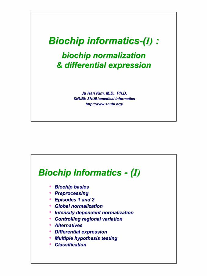
Biochip informatics Biochip informatics-( I) I) : biochip normalization biochip normalization & differential expression & differential expression Ju Han Kim, M.D., Ph.D. Ju Han Kim, M.D., Ph.D. SNUBI: SNUBI: SNUBiomedical SNUBiomedical Informatics Informatics http://www. http://www. snubi snubi .org/ .org/ Biochip Informatics Biochip Informatics -( I) I) • Biochip basics Biochip basics • Preprocessing Preprocessing • Episodes 1 and 2 Episodes 1 and 2 • Global normalization Global normalization • Intensity dependent normalization Intensity dependent normalization • Controlling regional variation Controlling regional variation • Alternatives Alternatives • Differential expression Differential expression • Multiple hypothesis testing Multiple hypothesis testing • Classification Classification
-
Upload
phungkhanh -
Category
Documents
-
view
240 -
download
1
Transcript of Biochip informatics-(I) - snubi.orgjuhan/BGM/ppt/MG_BiochipInformatics.pdf · Biochip...
1
Biochip informaticsBiochip informatics--((I)I) ::biochip normalization biochip normalization
& differential expression& differential expression
Ju Han Kim, M.D., Ph.D.Ju Han Kim, M.D., Ph.D.SNUBI: SNUBI: SNUBiomedicalSNUBiomedical InformaticsInformatics
http://www.http://www.snubisnubi.org/.org/
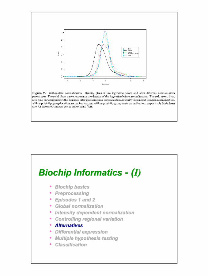
Biochip InformaticsBiochip Informatics -- ((I)I)•• Biochip basicsBiochip basics•• PreprocessingPreprocessing•• Episodes 1 and 2Episodes 1 and 2•• Global normalizationGlobal normalization•• Intensity dependent normalizationIntensity dependent normalization•• Controlling regional variationControlling regional variation•• AlternativesAlternatives•• Differential expressionDifferential expression•• Multiple hypothesis testingMultiple hypothesis testing•• ClassificationClassification

2
Biochip basicsBiochip basics
Bioinformaticspipeline
TerminologyTerminology• Sample (Target): RNA (cDNA) hybridized to the array,
aka target, mobile substrate.• Probe: DNA spotted on the array, aka spot, immobile
substrate.• Sector (Block): rectangular matrix of spots printed using
the same print-tip (or pin), aka print-tip-group• Slide, Array: printed microarray• Batch: collection of microarrays with the same probe
layout.• Channel: data from one color (Cy3 = cyanine 3 = green,
Cy5 = cyanine 5 = red).
3
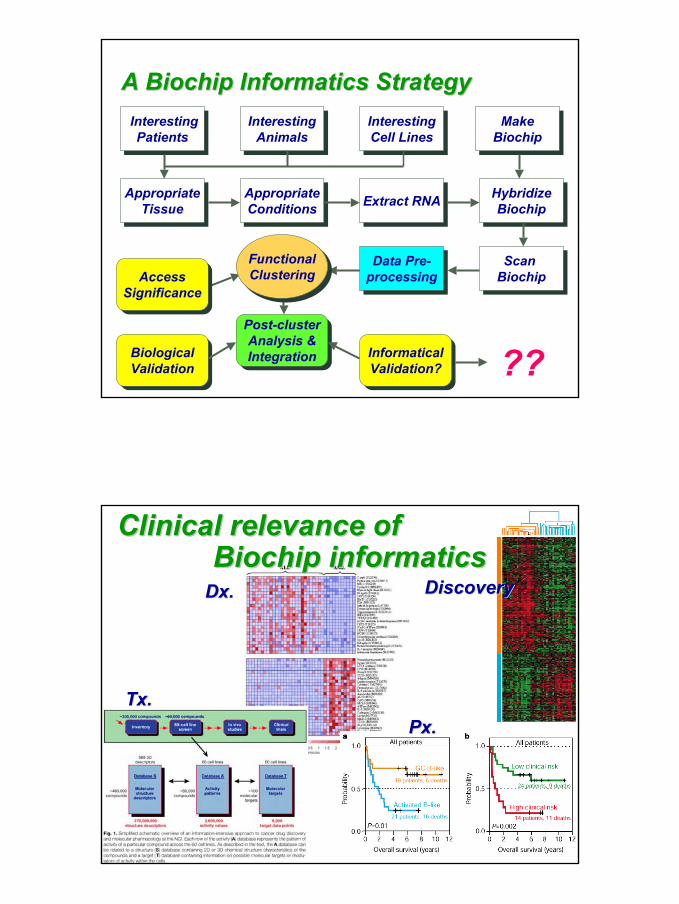
InterestingPatients
InterestingPatients
InterestingAnimals
InterestingAnimals
InterestingCell Lines
InterestingCell Lines
AppropriateTissue
AppropriateTissue
AppropriateConditions
AppropriateConditions Extract RNAExtract RNA
Scan BiochipScan
Biochip
HybridizeBiochip
HybridizeBiochip
MakeBiochipMake
Biochip
Data Pre-processingData Pre-
processing
A Biochip Informatics StrategyA Biochip Informatics Strategy
Post-clusterAnalysis &Integration
Post-clusterAnalysis &IntegrationBiological
ValidationBiologicalValidation
InformaticalValidation?
InformaticalValidation? ??
FunctionalClustering
FunctionalClusteringAccess
SignificanceAccess
Significance
Clinical relevance of Clinical relevance of Biochip informaticsBiochip informatics
DxDx.. DiscoveryDiscovery
PxPx..TxTx..
4
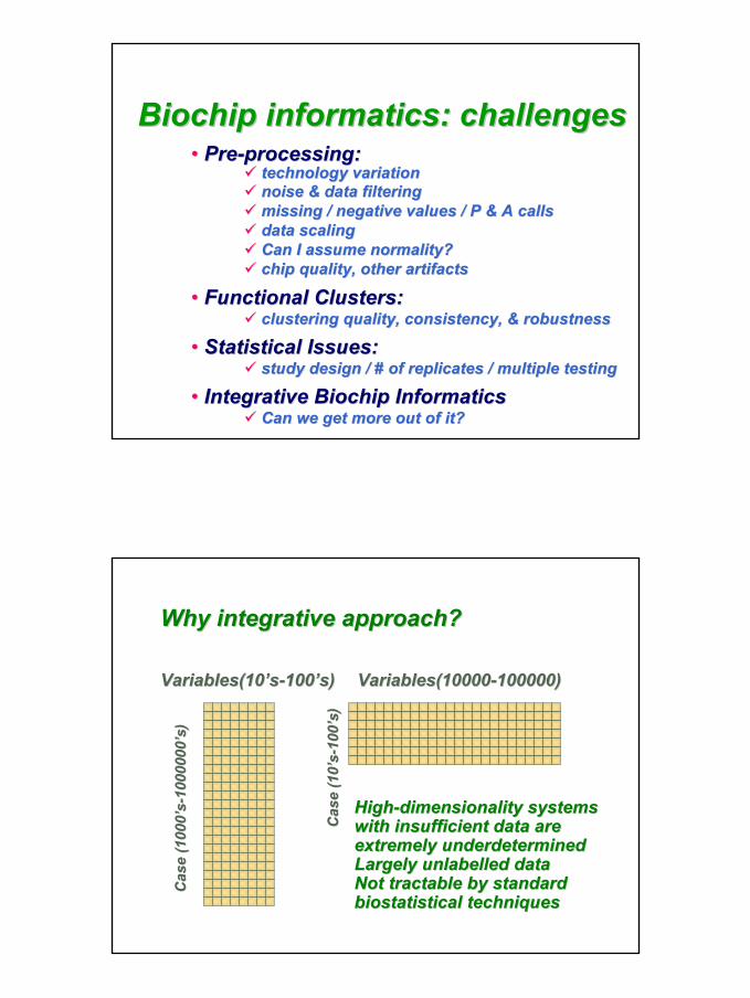
Biochip informatics: challengesBiochip informatics: challenges•• PrePre--processing:processing:
technology variationtechnology variationnoise & data filteringnoise & data filteringmissing / negative values / P & A callsmissing / negative values / P & A callsdata scalingdata scalingCan I assume normality?Can I assume normality?chip quality, other artifactschip quality, other artifacts
•• Functional Clusters: Functional Clusters: clustering quality, consistency, & robustnessclustering quality, consistency, & robustness
•• Statistical Issues: Statistical Issues: study design / # of replicates / multiple testingstudy design / # of replicates / multiple testing
•• Integrative Biochip InformaticsIntegrative Biochip InformaticsCan we get more out of it?Can we get more out of it?
Why integrative approach?Why integrative approach?
Variables(10Variables(10’’ss--100100’’s)s) Variables(10000Variables(10000--100000)100000)
Cas
e (1
000
Cas
e (1
000 ’’
ss --10
0000
010
0000
0 ’’s)s)
Cas
e (1
0C
ase
(10 ’’
ss --10
010
0 ’’s)s)
HighHigh--dimensionality systems dimensionality systems with insufficient data are with insufficient data are extremely underdeterminedextremely underdeterminedLargely unlabelled dataLargely unlabelled dataNot tractable by standard Not tractable by standard biostatisticalbiostatistical techniquestechniques
5
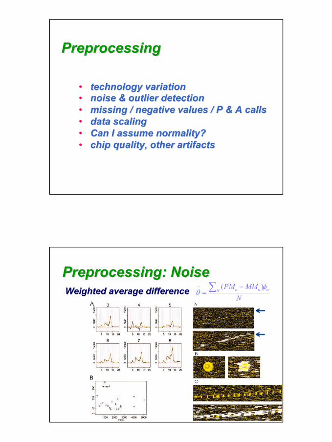
PreprocessingPreprocessing
•• technology variationtechnology variation•• noise & outlier detectionnoise & outlier detection•• missing / negative values / P & A callsmissing / negative values / P & A calls•• data scalingdata scaling•• Can I assume normality?Can I assume normality?•• chip quality, other artifactschip quality, other artifacts
Preprocessing: NoisePreprocessing: NoiseWeighted average differenceWeighted average difference
NMMPM nN nn φ
θ ∑ −=
)(~
6
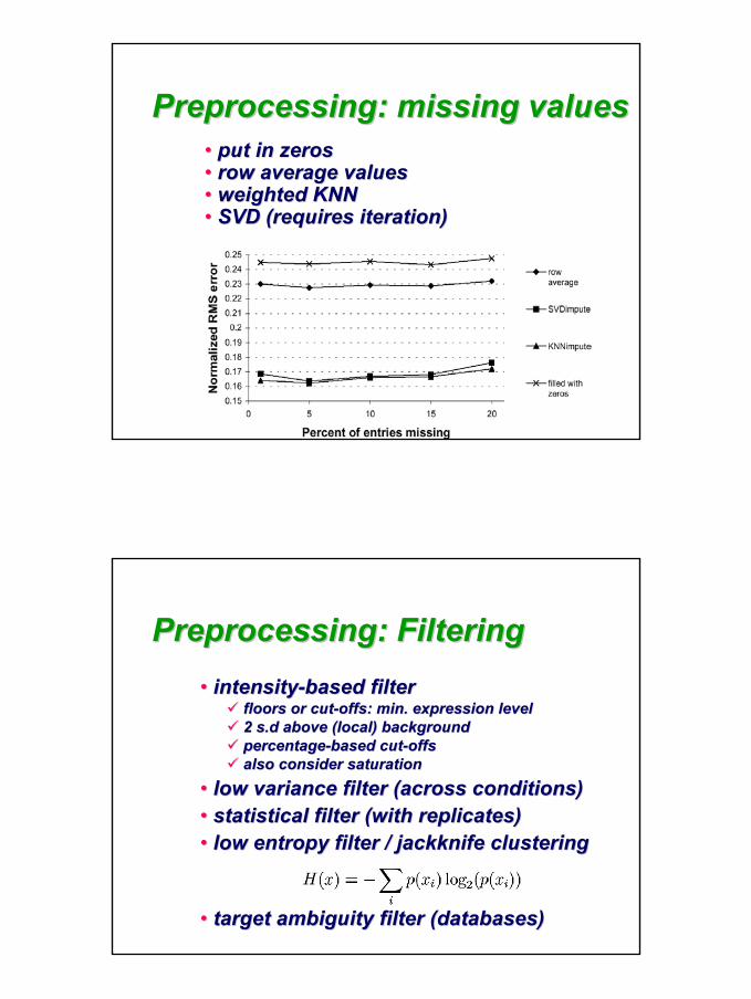
Preprocessing: missing valuesPreprocessing: missing values•• put in zerosput in zeros•• row average valuesrow average values•• weighted KNNweighted KNN•• SVD (requires iteration)SVD (requires iteration)
•• intensityintensity--based filterbased filterfloors or cutfloors or cut--offs: min. expression leveloffs: min. expression level2 s.d above (local) background2 s.d above (local) backgroundpercentagepercentage--based cutbased cut--offsoffsalso consider saturationalso consider saturation
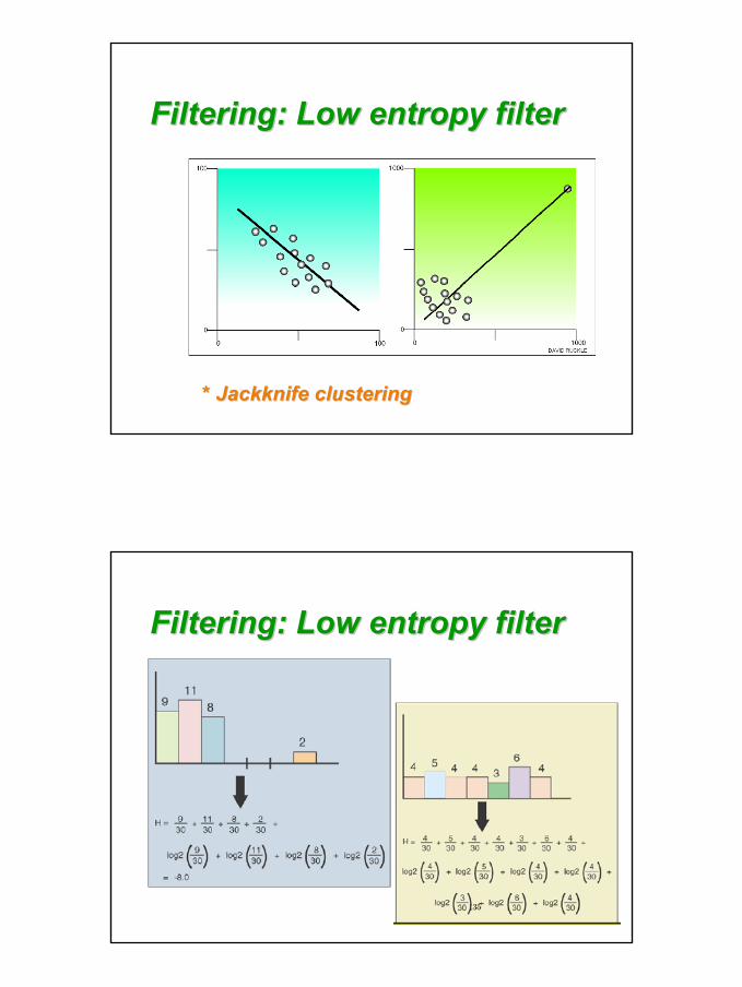
•• low variance filter (across conditions)low variance filter (across conditions)•• statistical filter (with replicates)statistical filter (with replicates)•• low entropy filter / jackknife clusteringlow entropy filter / jackknife clustering
•• target ambiguity filter (databases)target ambiguity filter (databases)
Preprocessing: FilteringPreprocessing: Filtering
7
Filtering: Low entropy filterFiltering: Low entropy filter
** Jackknife clusteringJackknife clustering
Filtering: Low entropy filterFiltering: Low entropy filter
8
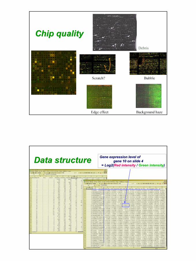
Chip qualityChip qualityDebris
Data structureData structure Gene expression level of Gene expression level of gene 10 on slide 4gene 10 on slide 4
= Log2(= Log2(Red intensityRed intensity / / Green intensityGreen intensity))
9
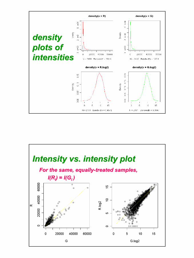
density density plots ofplots ofintensitiesintensities
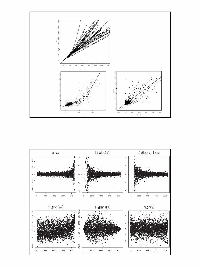
Intensity vs. intensity plotIntensity vs. intensity plotFor the same, equallyFor the same, equally--treated samples, treated samples,
I(I(RRii) = I() = I(GGii ))
10
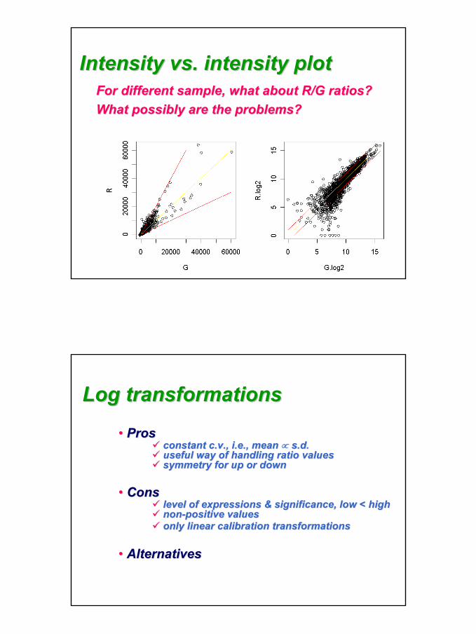
Intensity vs. intensity plotIntensity vs. intensity plotFor different sample, what about R/G ratios?For different sample, what about R/G ratios?What possibly are the problems? What possibly are the problems?
Log transformationsLog transformations
•• ProsProsconstant c.v., i.e., mean constant c.v., i.e., mean ∝∝ s.d.s.d.useful way of handling ratio valuesuseful way of handling ratio valuessymmetry for up or downsymmetry for up or down
•• ConsConslevel of expressions & significance, low < highlevel of expressions & significance, low < highnonnon--positive valuespositive valuesonly linear calibration transformationsonly linear calibration transformations
•• AlternativesAlternatives
11
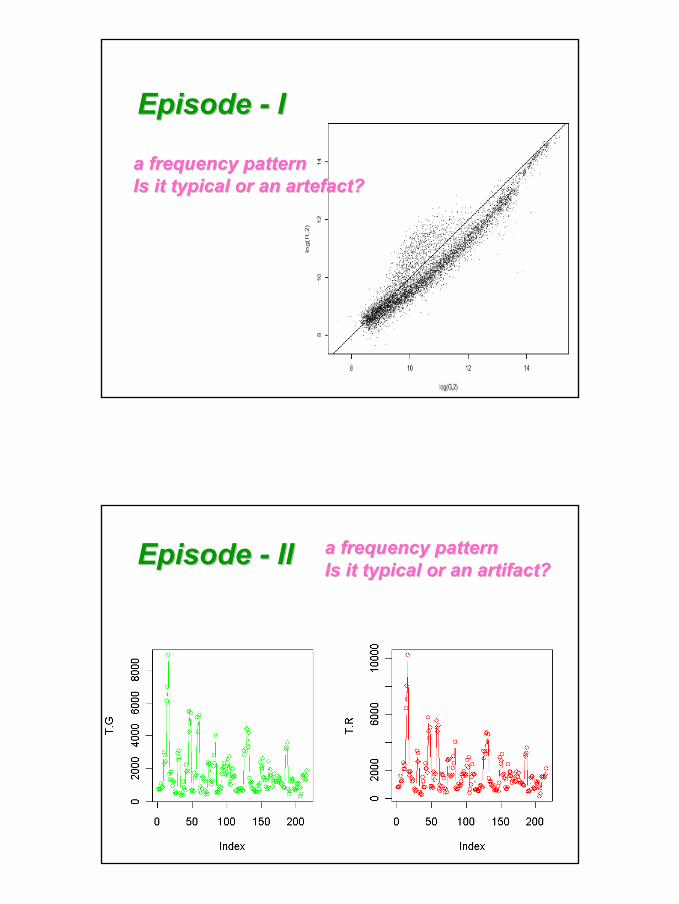
Episode Episode -- II
a frequency patterna frequency patternIs it typical or an Is it typical or an artefactartefact??
Episode Episode -- IIII a frequency patterna frequency patternIs it typical or an artifact?Is it typical or an artifact?
12
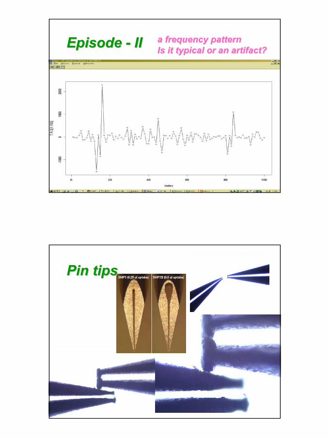
Episode Episode -- IIII a frequency patterna frequency patternIs it typical or an artifact?Is it typical or an artifact?
Pin tipsPin tips

13
NormalizationNormalizationCorrecting systematic variationCorrecting systematic variation•• Simple additive and multiplicativeSimple additive and multiplicative•• Linear vs. nonLinear vs. non--linearlinear•• Sources of errorSources of error•• Kinds?Kinds?
dyedyespottingspottingexperiment, slideexperiment, slidescale, scanningscale, scanning
14
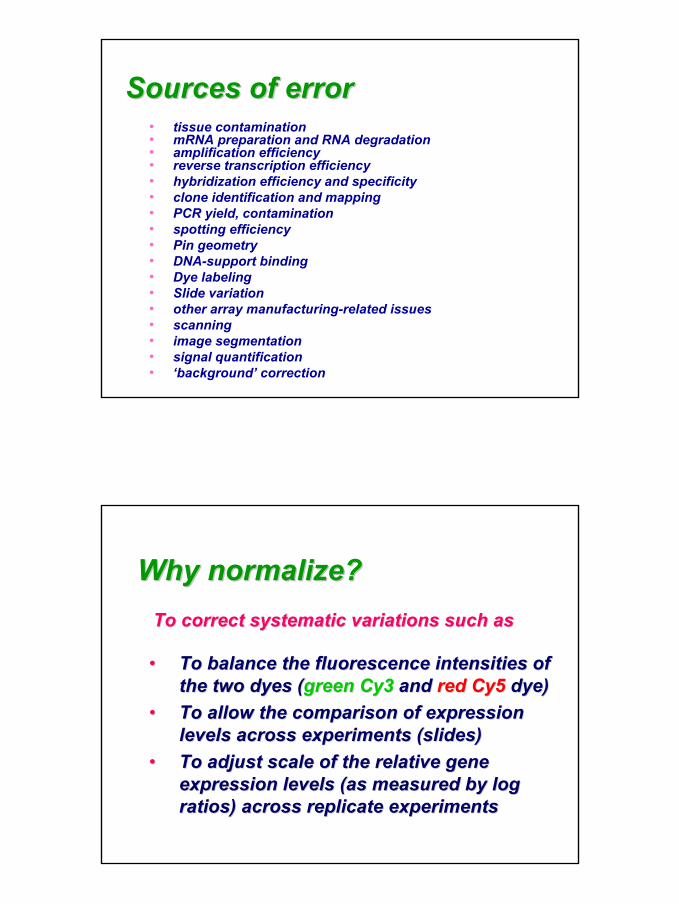
Sources of errorSources of error• tissue contamination• mRNA preparation and RNA degradation• amplification efficiency• reverse transcription efficiency• hybridization efficiency and specificity• clone identification and mapping• PCR yield, contamination• spotting efficiency• Pin geometry• DNA-support binding• Dye labeling• Slide variation• other array manufacturing-related issues• scanning• image segmentation• signal quantification• ‘background’ correction
•• To balance the fluorescence intensities of To balance the fluorescence intensities of the two dyes (the two dyes (green Cy3green Cy3 and and red Cy5red Cy5 dye)dye)
•• To allow the comparison of expression To allow the comparison of expression levels across experiments (slides)levels across experiments (slides)
•• To adjust scale of the relative gene To adjust scale of the relative gene expression levels (as measured by log expression levels (as measured by log ratios) across replicate experimentsratios) across replicate experiments
Why normalize?Why normalize?To correct systematic variations such asTo correct systematic variations such as
15
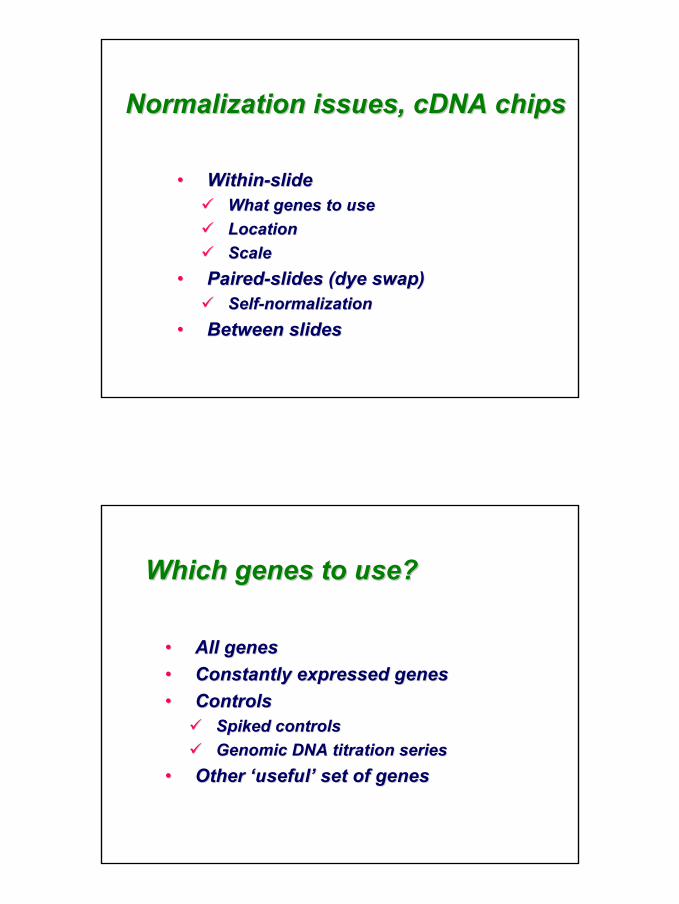
•• WithinWithin--slideslideWhat genes to useWhat genes to useLocationLocationScaleScale
•• PairedPaired--slides (dye swap)slides (dye swap)SelfSelf--normalizationnormalization
•• Between slidesBetween slides
Normalization issues, Normalization issues, cDNA cDNA chipschips
•• All genesAll genes•• Constantly expressed genesConstantly expressed genes•• ControlsControls
Spiked controlsSpiked controlsGenomic DNA titration seriesGenomic DNA titration series
•• Other Other ‘‘usefuluseful’’ set of genesset of genes
Which genes to use?Which genes to use?
16
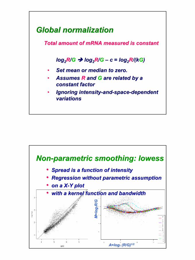
loglog22RR//GG loglog22RR//GG –– c = logc = log22RR/(/(kkGG))
•• Set mean or median to zero.Set mean or median to zero.•• Assumes Assumes RR and and GG are related by a are related by a
constant factorconstant factor•• Ignoring intensityIgnoring intensity--andand--spacespace--dependent dependent
variationsvariations
Global normalizationGlobal normalizationTotal amount of Total amount of mRNAmRNA measured is constantmeasured is constant
M=l
ogM
=log
22 R/GR/G
A=logA=log22 (R/G)(R/G)1/21/2
NonNon--parametric smoothing: parametric smoothing: lowesslowess•• Spread is a function of intensitySpread is a function of intensity•• Regression without parametric assumptionRegression without parametric assumption•• on a Xon a X--Y plotY plot•• with a kernel function and bandwidthwith a kernel function and bandwidth
17
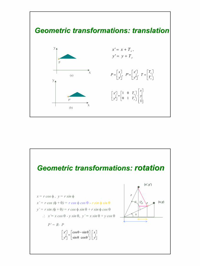
Geometric transformations: translationGeometric transformations: translation
=
=
=
y
x
TT
Tyx
Pyx
P ,''
',
x
y
x
y
(b)
(a)
P
P’
⋅
=
11001
''
yx
TT
yx
y
x
y
x
Ty'y,Tx'x
+=+=
Geometric transformations: Geometric transformations: rotationrotation
x = r cos φ , y = r sin φ
x’ = r cos (φ + θ) = r cos φ cos θ - r sin φ sin θ
y’ = r sin (φ + θ) = r cos φ sin θ + r sin φ cos θ
∴ x’= x cos θ - y sin θ, y’ = x sin θ + y cos θ
P’ = R⋅ P
⋅
θθ−
θθ
=
yx
yx
cossin
sincos
''
(x,y)
r
φ
(x’,y’)
rθ
18
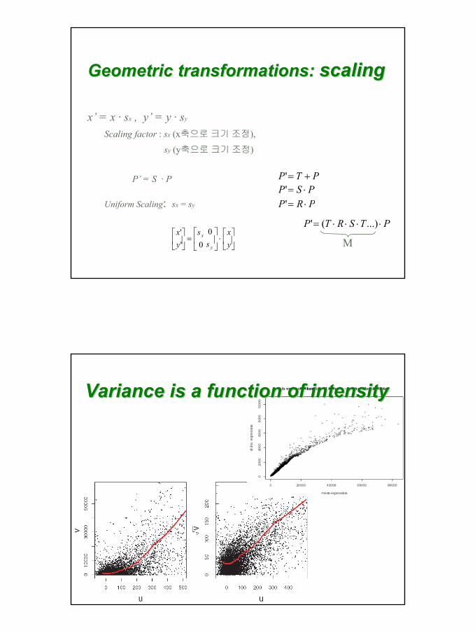
Geometric transformations: Geometric transformations: scalingscaling
x’ = x · sx , y’ = y · sy
Scaling factor : sx (x축으로크기조정),
sy (y축으로크기조정)
P’ = S · P
Uniform Scaling: sx = sy
⋅
=
yx
ss
yx
y
x 00'
'
PTP +='PSP ⋅='PRP ⋅='
PTSRTP ⋅⋅⋅⋅= ...)('
M
Variance is a function of intensityVariance is a function of intensity
19
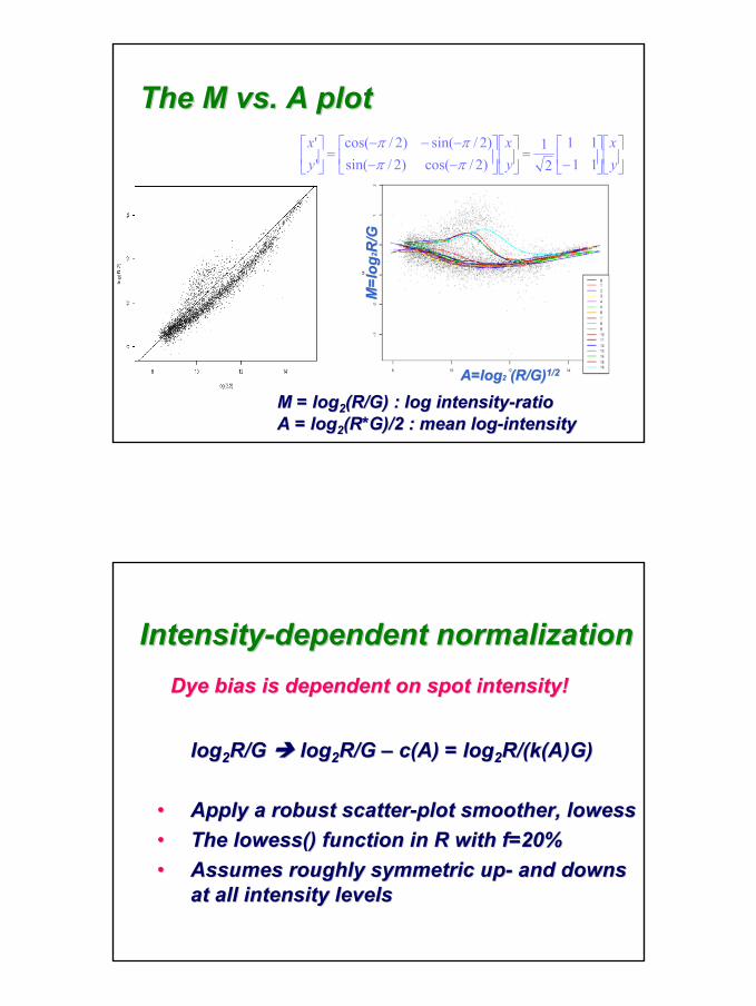
The M vs. A plotThe M vs. A plot
M = logM = log22(R/G) : log intensity(R/G) : log intensity--ratioratioA = logA = log22(R*G)/2 : mean log(R*G)/2 : mean log--intensityintensity
M=l
ogM
=log
22 R/GR/G
A=logA=log22 (R/G)(R/G)1/21/2
−
=
−−−−−
=
yx
yx
yx
1111
21
)2/cos()2/sin()2/sin()2/cos(
''
ππππ
loglog22R/G R/G loglog22R/G R/G –– c(A) = logc(A) = log22R/(k(A)G)R/(k(A)G)
•• Apply a robust scatterApply a robust scatter--plot smoother, plot smoother, lowesslowess•• The The lowesslowess() function in R with f=20%() function in R with f=20%•• Assumes roughly symmetric upAssumes roughly symmetric up-- and downs and downs
at all intensity levelsat all intensity levels
IntensityIntensity--dependent normalizationdependent normalizationDye bias is dependent on spot intensity!Dye bias is dependent on spot intensity!
20
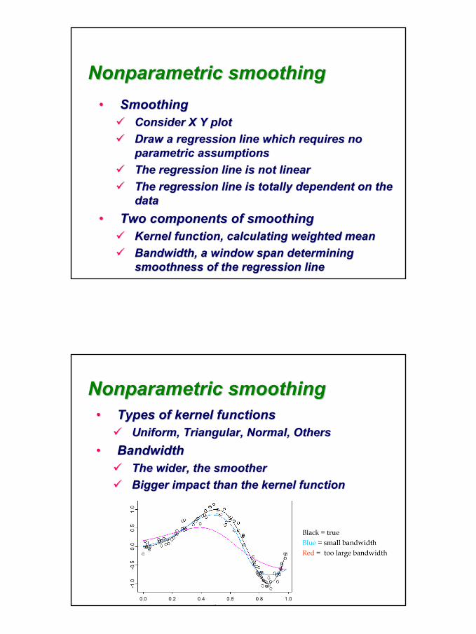
•• SmoothingSmoothingConsider X Y plotConsider X Y plotDraw a regression line which requires no Draw a regression line which requires no parametric assumptionsparametric assumptionsThe regression line is not linearThe regression line is not linearThe regression line is totally dependent on the The regression line is totally dependent on the datadata
•• Two components of smoothingTwo components of smoothingKernel function, calculating weighted meanKernel function, calculating weighted meanBandwidth, a window span determining Bandwidth, a window span determining smoothness of the regression linesmoothness of the regression line
Nonparametric smoothingNonparametric smoothing
•• Types of kernel functionsTypes of kernel functionsUniform, Triangular, Normal, OthersUniform, Triangular, Normal, Others
•• BandwidthBandwidthThe wider, the smootherThe wider, the smootherBigger impact than the kernel functionBigger impact than the kernel function
Nonparametric smoothingNonparametric smoothing
21
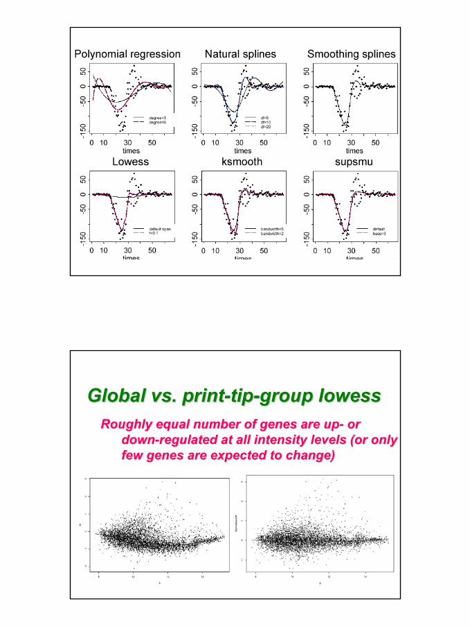
Roughly equal number of genes are upRoughly equal number of genes are up-- or or downdown--regulated at all intensity levels (or only regulated at all intensity levels (or only few genes are expected to change)few genes are expected to change)
Global vs. printGlobal vs. print--tiptip--group group lowesslowess
22
For every printFor every print--tip group, changes roughly tip group, changes roughly symmetric at all intensity levelssymmetric at all intensity levels
Global vs. printGlobal vs. print--tiptip--group group lowesslowess
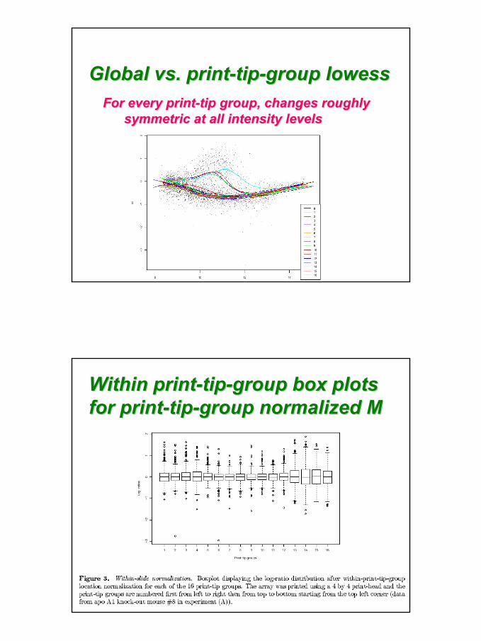
Within printWithin print--tiptip--group box plots group box plots for printfor print--tiptip--group normalized Mgroup normalized M
23
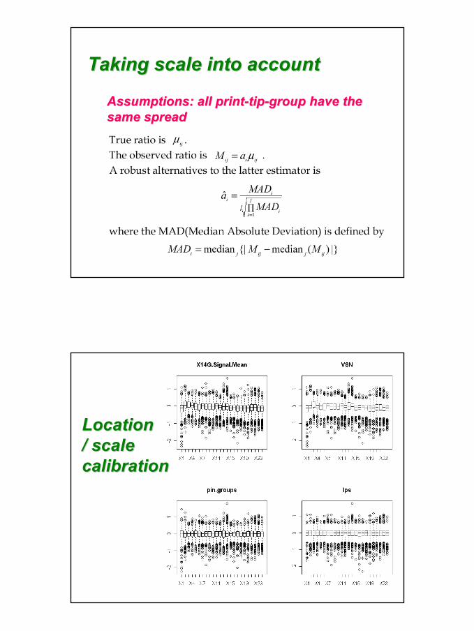
Taking scale into accountTaking scale into account
Assumptions: all printAssumptions: all print--tiptip--group have the group have the same spreadsame spread
Location Location / scale / scale calibrationcalibration
24
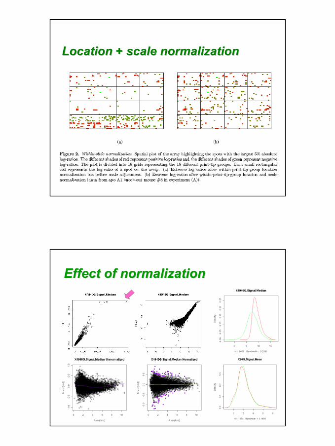
Location + scale normalizationLocation + scale normalization
Effect of normalizationEffect of normalization
25
Location + scale normalizationLocation + scale normalization
Biochip InformaticsBiochip Informatics -- ((I)I)•• Biochip basicsBiochip basics•• PreprocessingPreprocessing•• Episodes 1 and 2Episodes 1 and 2•• Global normalizationGlobal normalization•• Intensity dependent normalizationIntensity dependent normalization•• Controlling regional variationControlling regional variation•• AlternativesAlternatives•• Differential expressionDifferential expression•• Multiple hypothesis testingMultiple hypothesis testing•• ClassificationClassification
26
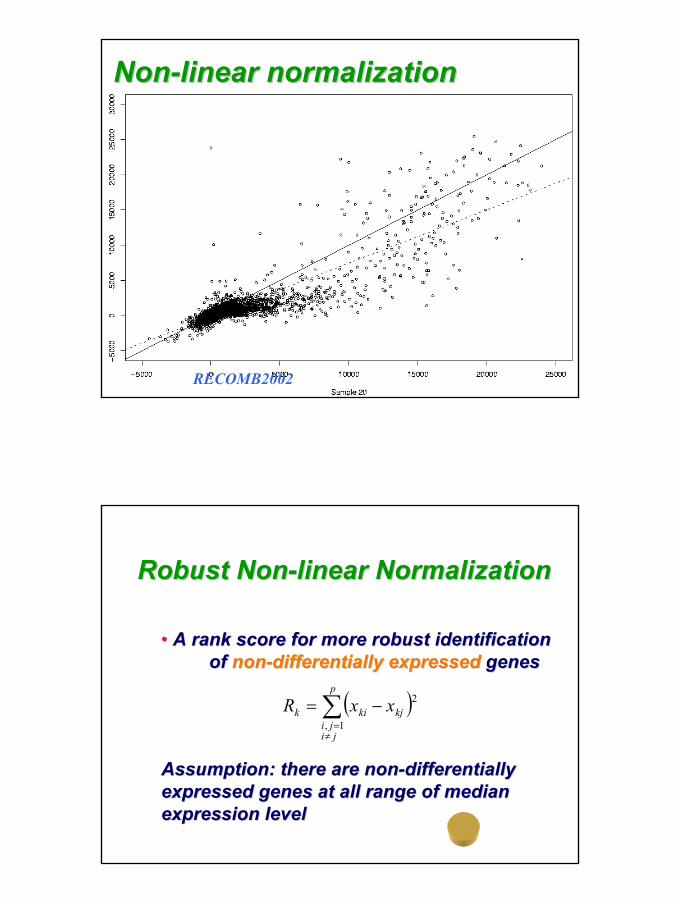
NonNon--linear normalizationlinear normalization
RECOMB2002
Robust NonRobust Non--linear Normalizationlinear Normalization
( )∑≠=
−=p
jiji
kjkik xxR1,
2
•• A rank score for more robust identification A rank score for more robust identification of of nonnon--differentially expresseddifferentially expressed genesgenes
Assumption: there are nonAssumption: there are non--differentially differentially expressed genes at all range of median expressed genes at all range of median expression level expression level
27
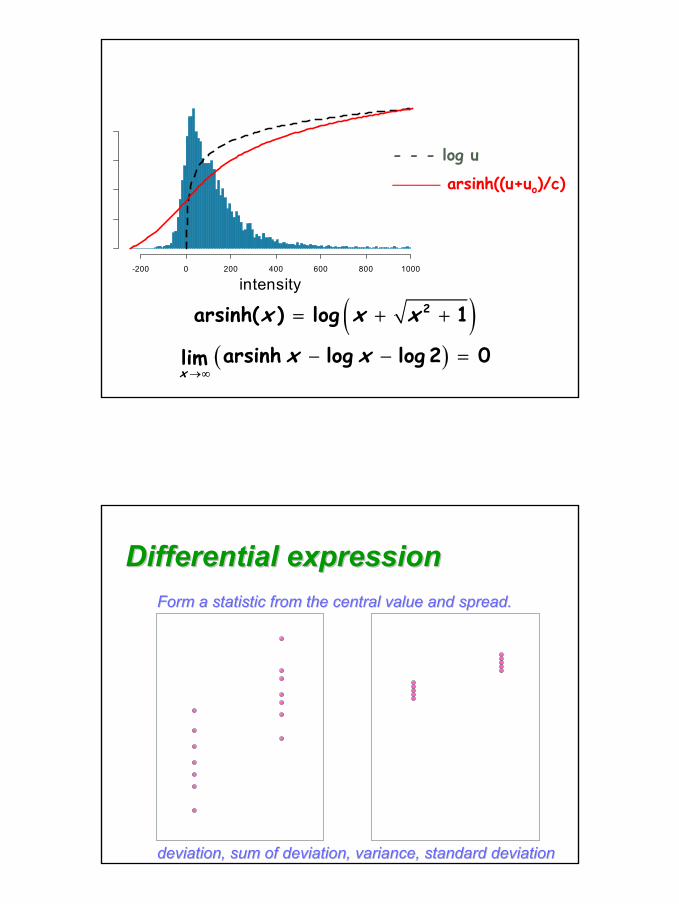
28
- - - log u
——— arsinh((u+uo)/c)
( )( )
2arsinh( ) log 1
arsinh log log 2 0limx
x x x
x x→∞
= + +
− − =
intensity-200 0 200 400 600 800 1000
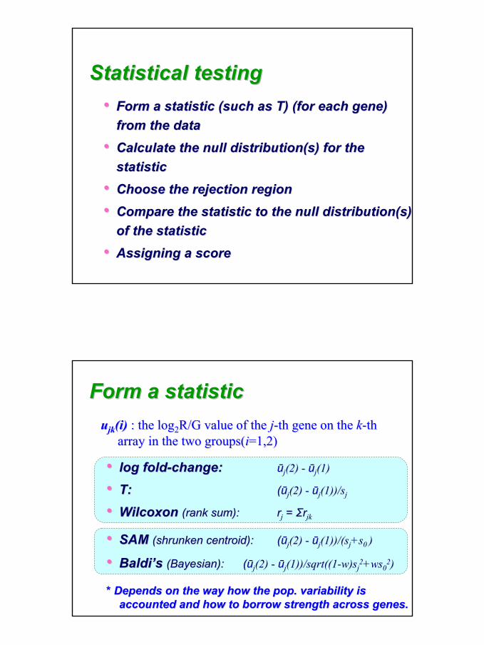
Differential expressionDifferential expression
deviation, sum of deviation, variance, standard deviationdeviation, sum of deviation, variance, standard deviation
Form a statistic from the central value and spread.Form a statistic from the central value and spread.
29
Statistical testingStatistical testing•• Form a statistic (such as T) (for each gene) Form a statistic (such as T) (for each gene)
from the datafrom the data•• Calculate the null distribution(s) for the Calculate the null distribution(s) for the
statisticstatistic•• Choose the rejection regionChoose the rejection region•• Compare the statistic to the null distribution(s) Compare the statistic to the null distribution(s)
of the statisticof the statistic•• Assigning a scoreAssigning a score
Form a statisticForm a statistic
•• log foldlog fold--change:change: ūūjj(2)(2) -- ūūjj(1)(1)
•• T:T: ((ūūjj(2)(2) -- ūūjj(1))/(1))/ssjj
•• WilcoxonWilcoxon (rank sum):(rank sum): rrjj = = ΣΣrrjkjk
•• SAM SAM (shrunken (shrunken centroidcentroid):): ((ūūjj(2)(2) -- ūūjj(1))/((1))/(ssjj+s+s0 0 ))
•• BaldiBaldi’’s s (Bayesian):(Bayesian): ((ūūjj(2)(2) -- ūūjj(1))/(1))/sqrtsqrt((1((1--w)sw)sjj22+ws+ws00
22))
* Depends on the way how the pop. variability is * Depends on the way how the pop. variability is accounted and how to borrow strength across genes.accounted and how to borrow strength across genes.
uujkjk(i)(i) : the log: the log22R/G value of the R/G value of the jj--th th gene on the gene on the kk--th th array in the two groups(array in the two groups(ii=1,2)=1,2)
30
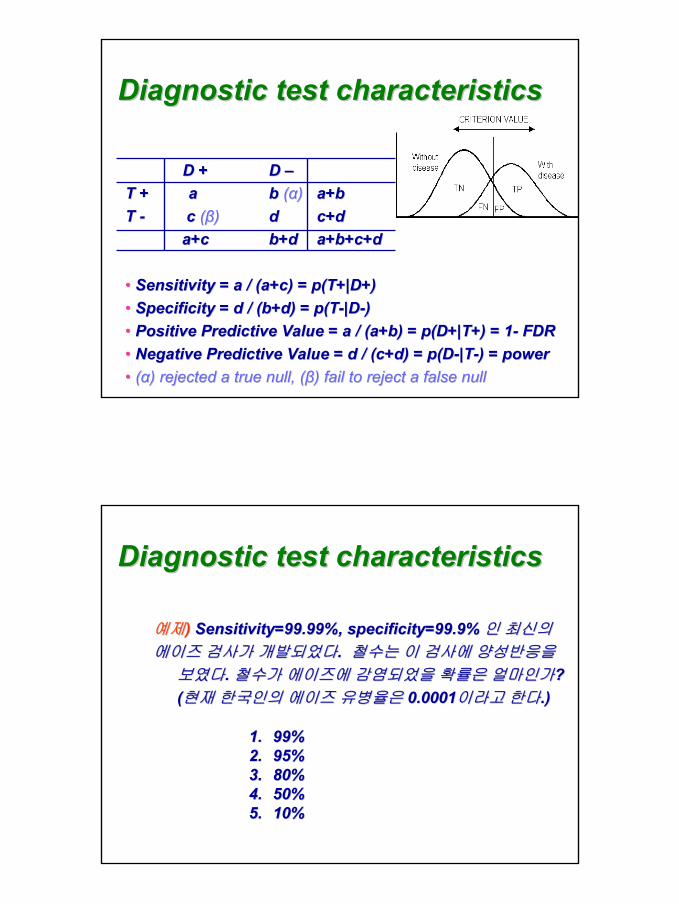
D +D + D D ––T + aT + a b b ((αα)) a+ba+bT T -- c c ((ββ)) dd c+dc+d
a+ca+c b+db+d a+b+c+da+b+c+d
•• Sensitivity = a / (a+c) = p(T+|D+)Sensitivity = a / (a+c) = p(T+|D+)•• Specificity = d / (b+d) = p(TSpecificity = d / (b+d) = p(T--|D|D--))•• Positive Predictive Value = a / (a+b) = p(D+|T+) = 1Positive Predictive Value = a / (a+b) = p(D+|T+) = 1-- FDRFDR•• Negative Predictive Value = d / (c+d) = p(DNegative Predictive Value = d / (c+d) = p(D--|T|T--) = power) = power•• ((αα) rejected a true null, () rejected a true null, (ββ) fail to reject a false null) fail to reject a false null
Diagnostic test characteristics Diagnostic test characteristics
예제예제)) Sensitivity=99.99%, specificity=99.9% Sensitivity=99.99%, specificity=99.9% 인인 최신의최신의
에이즈에이즈 검사가검사가 개발되었다개발되었다. . 철수는철수는 이이 검사에검사에 양성반응을양성반응을
보였다보였다. . 철수가철수가 에이즈에에이즈에 감염되었을감염되었을 확률은확률은 얼마인가얼마인가? ? ((현재현재 한국인의한국인의 에이즈에이즈 유병율은유병율은 0.00010.0001이라고이라고 한다한다.).)
1.1. 99%99%2.2. 95%95%3.3. 80%80%4.4. 50%50%5.5. 10%10%
Diagnostic test characteristics Diagnostic test characteristics
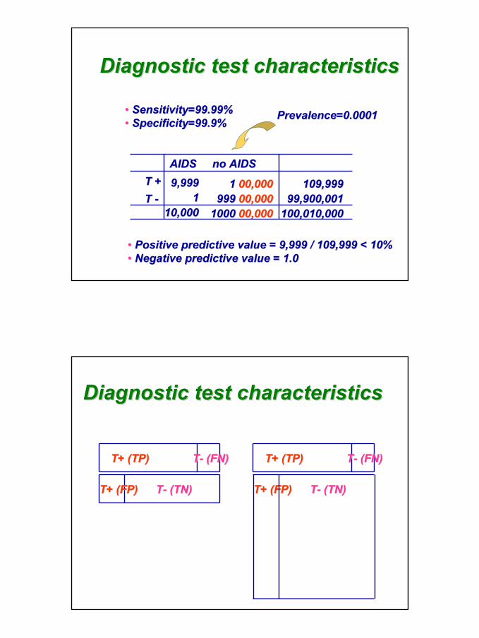
31
Diagnostic test characteristics Diagnostic test characteristics
AIDS AIDS no AIDSno AIDST +T +T T --
9,9999,99911
10,00010,000
•• Sensitivity=99.99%Sensitivity=99.99%•• Specificity=99.9%Specificity=99.9%
11999 999
10001000
Prevalence=0.0001Prevalence=0.0001
00,00000,00000,000 00,000 00,00000,000
109,999109,99999,900,00199,900,001
100,010,000100,010,000
•• Positive predictive value = 9,999 / 109,999 < 10%Positive predictive value = 9,999 / 109,999 < 10%•• Negative predictive value = 1.0Negative predictive value = 1.0
T+ (TP)T+ (TP) TT-- (FN)(FN)
T+ (FP)T+ (FP) TT-- (TN)(TN)
T+ (TP)T+ (TP) TT-- (FN)(FN)
T+ (FP)T+ (FP) TT-- (TN)(TN)
Diagnostic test characteristics Diagnostic test characteristics
32
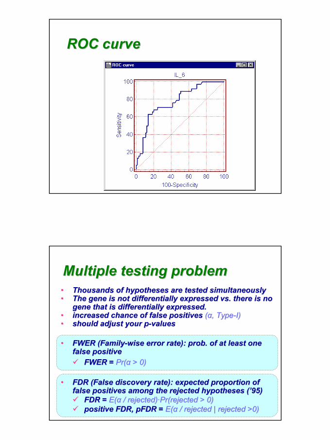
ROC curveROC curve
•• Thousands of hypotheses are tested simultaneouslyThousands of hypotheses are tested simultaneously•• The gene is not differentially expressed vs. there is no The gene is not differentially expressed vs. there is no
gene that is differentially expressed.gene that is differentially expressed.•• increased chance of false positives increased chance of false positives ((αα, Type, Type--II) ) •• should adjust your pshould adjust your p--valuesvalues
•• FWER (FamilyFWER (Family--wise error rate): prob. of at least one wise error rate): prob. of at least one false positivefalse positive
FWER = FWER = Pr(Pr(αα > 0)> 0)
•• FDR (False discovery rate): expected proportion of FDR (False discovery rate): expected proportion of false positives among the rejected hypotheses (false positives among the rejected hypotheses (’’95)95)
FDR = FDR = E(E(αα / rejected)/ rejected)··Pr(rejected > 0)Pr(rejected > 0)positive FDR,positive FDR, pFDRpFDR = = E(E(αα / rejected | rejected >0)/ rejected | rejected >0)
Multiple testing problemMultiple testing problem
33
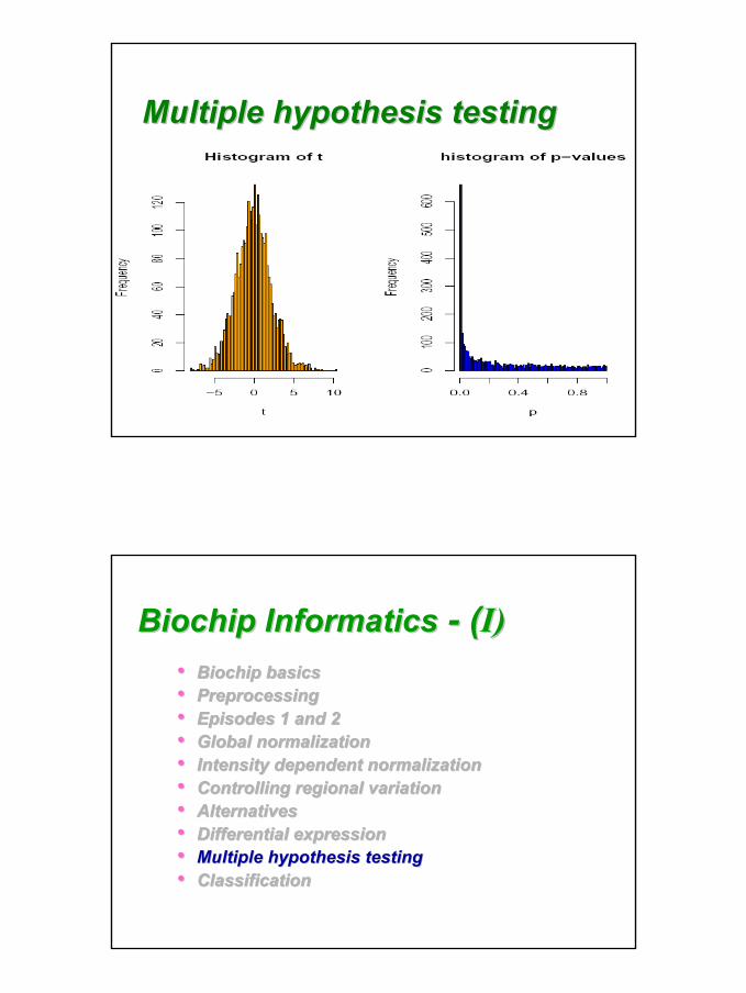
Multiple hypothesis testingMultiple hypothesis testing
Biochip InformaticsBiochip Informatics -- ((I)I)•• Biochip basicsBiochip basics•• PreprocessingPreprocessing•• Episodes 1 and 2Episodes 1 and 2•• Global normalizationGlobal normalization•• Intensity dependent normalizationIntensity dependent normalization•• Controlling regional variationControlling regional variation•• AlternativesAlternatives•• Differential expressionDifferential expression•• Multiple hypothesis testingMultiple hypothesis testing•• ClassificationClassification
34
•• Microarray experiments are large and exploratoryMicroarray experiments are large and exploratory•• 5% of FDR says that, among the 100 genes said 5% of FDR says that, among the 100 genes said
significant about 95 may be truly significant.significant about 95 may be truly significant.•• What dose 5% of FWER in microarray experiments?What dose 5% of FWER in microarray experiments?•• …… and compared to the top (arbitrary) 100 list?and compared to the top (arbitrary) 100 list?•• What about symmetric vs. asymmetric rejection What about symmetric vs. asymmetric rejection
regions?regions?•• Robustness against the kind of dependence?Robustness against the kind of dependence?•• ……..
Multiple testing in microarrayMultiple testing in microarray
•• complete null hypothesis that there is no gene that complete null hypothesis that there is no gene that is differentially expressed (i.e., a+c = a+b+c+d)is differentially expressed (i.e., a+c = a+b+c+d)
•• weak control of typeweak control of type--I errorI errorFWER = FWER = Pr(Pr(αα > 0) = Pr(at least one adjusted p> 0) = Pr(at least one adjusted pgg < c|H< c|H00))
•• ? dependence structure? dependence structure
Control of the FWERControl of the FWERBonferroniBonferroni correctioncorrection
•• by reby re--samplingsampling•• strong control of typestrong control of type--I error (i.e., regardless of a+c)I error (i.e., regardless of a+c)•• stepstep--down proceduredown procedure•• maxTmaxT
Westfall/YoungWestfall/Young’’s s minP minP adjusted padjusted p--valuesvalues
35
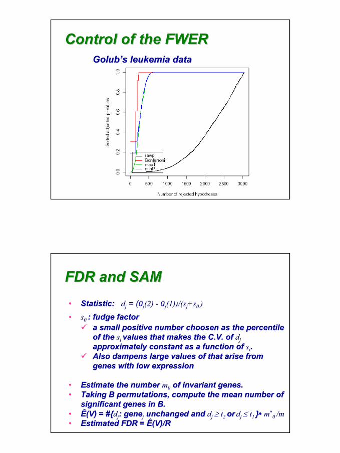
Control of the FWERControl of the FWERGolubGolub’’s s leukemia dataleukemia data
•• Statistic:Statistic: ddjj = (= (ūūjj(2)(2) -- ūūjj(1))/((1))/(ssjj+s+s0 0 ))
•• ss0 0 : fudge factor: fudge factora small positive number a small positive number choosen choosen as the percentile as the percentile of the of the ssii values that makes the C.V. of values that makes the C.V. of ddj j approximately constant as a function of approximately constant as a function of ssii..Also dampens large values of that arise from Also dampens large values of that arise from genes with low expressiongenes with low expression
•• Estimate the number Estimate the number mm00 of invariant genes.of invariant genes.•• Taking B permutations, compute the mean number of Taking B permutations, compute the mean number of
significant genes in B. significant genes in B. •• ÊÊ(V) = #{(V) = #{ddjj: : genegenejj unchanged and unchanged and ddjj ≥≥ tt2 2 oror ddj j ≤≤ tt1 1 }}•• mm**
0 0 /m/m•• Estimated FDR = Estimated FDR = ÊÊ(V)/R(V)/R
FDR and SAMFDR and SAM
36
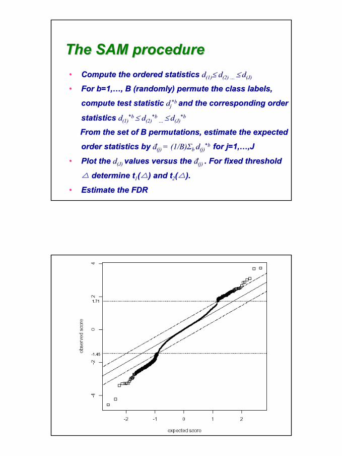
•• Compute the ordered statistics Compute the ordered statistics dd(1)(1)≤≤ dd(2) (2) …… ≤≤ dd(J)(J)
•• For b=1,For b=1,……, B (randomly) permute the class labels, , B (randomly) permute the class labels,
compute test statistic compute test statistic ddjj*b *b and the corresponding order and the corresponding order
statistics statistics dd(1)(1)*b*b ≤≤ dd(2)(2)
*b*b…… ≤≤ dd(J)(J)
*b*b
From the set of B permutations, estimate the expected From the set of B permutations, estimate the expected
order statistics by order statistics by đđ(j) (j) = (1/B)= (1/B)ΣΣbb dd(j)(j)*b *b for j=1,for j=1,……,J,J
•• Plot the Plot the dd(J) (J) values versus the values versus the đđ(j) (j) . For fixed threshold . For fixed threshold
△△ determine tdetermine t11((△△) and t) and t22((△△).).
•• Estimate the FDREstimate the FDR
The SAM procedureThe SAM procedure
37
Molecular Classification of CancerMolecular Classification of Cancer
GolbeGolbe, et al., Science, et al., Science1999;403:5031999;403:503--511511
38
Machine Learning Approach in Bioinformatics
•• Supervised Machine LearningSupervised Machine Learning
•• Linear Linear Discriminant Discriminant Analysis / Logistic Regression / PCAAnalysis / Logistic Regression / PCA•• Classification TreeClassification Tree•• Artificial Neural NetworkArtificial Neural Network•• Support Vector MachineSupport Vector Machine•• Rough SetsRough Sets•• Reinforcement LearningReinforcement Learning•• Hidden Markov ModelHidden Markov Model
•• Unsupervised Machine LearningUnsupervised Machine Learning
•• Hierarchical Tree ClusteringHierarchical Tree Clustering•• Partitional ClusteringPartitional Clustering•• SelfSelf--Organizing Feature MapsOrganizing Feature Maps•• Matrix Incision AlgorithmsMatrix Incision Algorithms
Supervised Supervised vsvs unsupervised classificationsunsupervised classifications
ClassificationConditional DensitiesClassificationClassification
Conditional DensitiesConditional Densities
knownknownknown unknownunknownunknown
Bayes DecisionTheory
Bayes Bayes DecisionDecisionTheoryTheory
SupervisedLearning
SupervisedSupervisedLearningLearning
UnsupervisedLearning
UnsupervisedUnsupervisedLearningLearning
ParametricParametricParametric NonparametricNonparametricNonparametric
“Optimal”Rules
““OptimalOptimal””RulesRules
Plug-inRules
PlugPlug--ininRulesRules
DensityEstimationDensityDensity
EstimationEstimationDecisionBoundaryBuilding
DecisionDecisionBoundaryBoundaryBuildingBuilding
MixtureResolvingMixtureMixture
ResolvingResolvingCluster
AnalysisClusterCluster
AnalysisAnalysis
ParametricParametricParametric NonparametricNonparametricNonparametric
Jain Jain et al. 2000, IEEE Transactionset al. 2000, IEEE Transactions
DensityDensity--basedbased
geometricgeometric
39
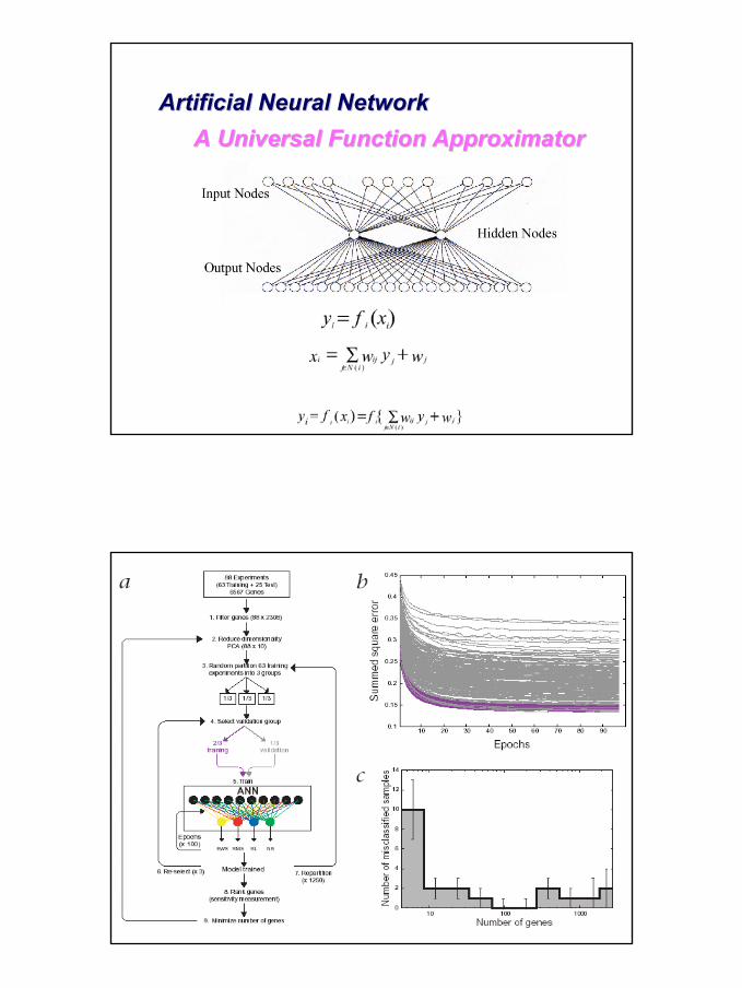
Artificial Neural NetworkArtificial Neural NetworkA Universal Function A Universal Function ApproximatorApproximator
40
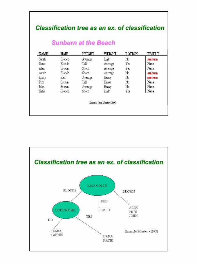
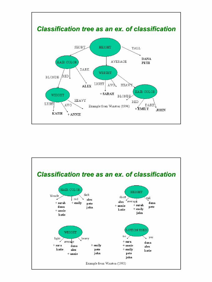
Classification tree as an ex. of classificationClassification tree as an ex. of classification
Sunburn at the BeachSunburn at the Beach
Classification tree as an ex. of classificationClassification tree as an ex. of classification
41
Classification tree as an ex. of classificationClassification tree as an ex. of classification
Classification tree as an ex. of classificationClassification tree as an ex. of classification
42
Classification tree as an ex. of classificationClassification tree as an ex. of classification
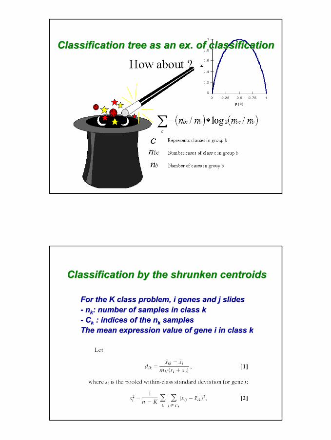
Classification by the shrunken centroidsClassification by the shrunken centroids
For the K class problem, i genes and j slidesFor the K class problem, i genes and j slides-- nnkk: number of samples in class k: number of samples in class k-- CCkk : indices of the : indices of the nnkk samplessamplesThe mean expression value of gene i in class kThe mean expression value of gene i in class k

43
shrunken shrunken centroidscentroids
classificationclassificationexerciseexercise
44
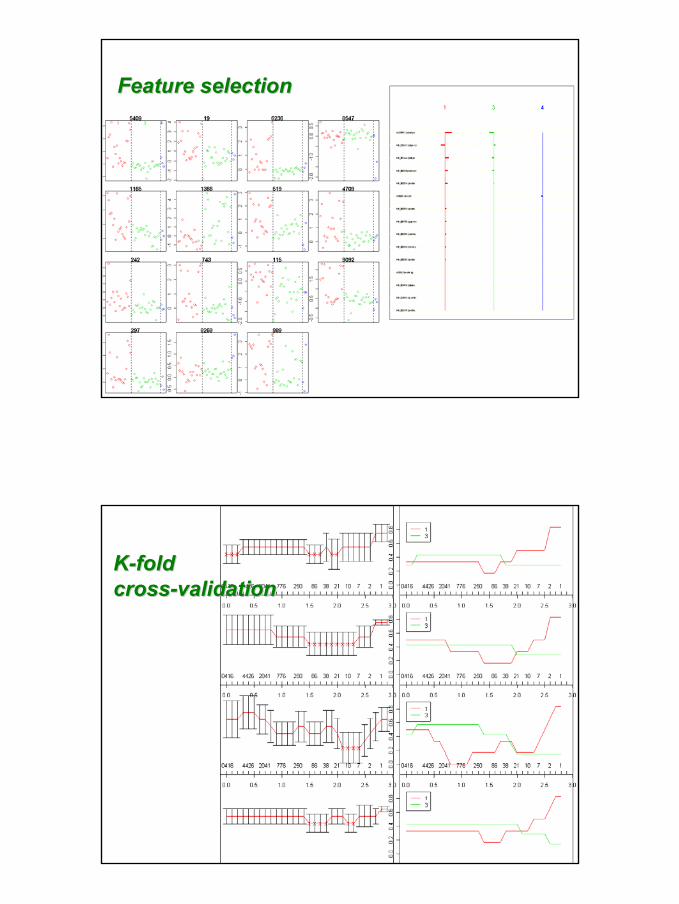
Feature selectionFeature selection
KK--fold fold crosscross--validationvalidation
45
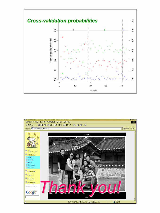
CrossCross--validation probabilitiesvalidation probabilities
Thank you!Thank you!