Binary intersymbol interference channels: gallager codes ...michaelm/postscripts/toit2003a.pdf ·...
17
1636 IEEE TRANSACTIONS ON INFORMATION THEORY, VOL. 49, NO. 7, JULY 2003 Binary Intersymbol Interference Channels: Gallager Codes, Density Evolution, and Code Performance Bounds Aleksandar Kavˇ cic ´ , Member, IEEE, Xiao Ma, and Michael Mitzenmacher, Member, IEEE Abstract—We study the limits of performance of Gallager codes (low-density parity-check (LDPC) codes) over binary linear inter- symbol interference (ISI) channels with additive white Gaussian noise (AWGN). Using the graph representations of the channel, the code, and the sum–product message-passing detector/decoder, we prove two error concentration theorems. Our proofs expand on previous work by handling complications introduced by the channel memory. We circumvent these problems by considering not just linear Gallager codes but also their cosets and by distin- guishing between different types of message flow neighborhoods depending on the actual transmitted symbols. We compute the noise tolerance threshold using a suitably developed density evolution algorithm and verify, by simulation, that the thresholds represent accurate predictions of the performance of the iterative sum–product algorithm for finite (but large) block lengths. We also demonstrate that for high rates, the thresholds are very close to the theoretical limit of performance for Gallager codes over ISI channels. If denotes the capacity of a binary ISI channel and if denotes the maximal achievable mutual information rate when the channel inputs are independent and identically distributed (i.i.d.) binary random variables , we prove that the maximum information rate achievable by the sum–product decoder of a Gallager (coset) code is upper-bounded by . The last topic investigated is the performance limit of the decoder if the trellis portion of the sum–product algorithm is executed only once; this demonstrates the potential for trading off the computational requirements and the performance of the decoder. Index Terms—Bahl–Cocke–Jelinek–Raviv (BCJR)-once bound, channel capacity, density evolution, Gallager codes, independent and identically distributed (i.i.d.) capacity, intersymbol interfer- ence (ISI) channel, low-density parity-check (LDPC) codes, sum– product algorithm, turbo equalization. I. INTRODUCTION I F continuous channel inputs are allowed, the capacity of discrete-time intersymbol interference (ISI) channels with additive white Gaussian noise (AWGN) can be computed using Manuscript received February 26, 2001; revised February 21, 2003. This work was supported by the National Science Foundation under Grants CCR-9904458 and CCR-0118701, and by the National Storage Industry Consortium. The material in this paper was presented in part at the IEEE International Symposium on Information Theory, Washington, DC, June 2001. A. Kavˇ cic ´ and M. Mitzenmacher are with the Division of Engineering and Applied Sciences, Harvard University, Cambridge, MA 02138 USA (e-mail: [email protected]; [email protected]). X. Ma was with the Division of Engineering and Applied Sciences, Harvard University, Cambridge, MA USA. He is now with the Department of Electrical Engineering, City University of Hong Kong, Kowloon, Hong Kong (e-mail: [email protected]). Communicated by R. Urbanke, Associate Editor for Coding Techniques. Digital Object Identifier 10.1109/TIT.2003.813563 the water-filling theorem [1], [2]. In many applications, the physics of the channel do not allow continuous input alphabets. A prime example of a two-level (binary) ISI channel is the saturation magnetic recording channel, because the magne- tization domains can have only two stable phases [3]. Other examples include digital communication channels where the input alphabet is confined to a finite set [4]. The computation of the capacity of discrete-time ISI chan- nels with a finite number of allowed signaling levels is an open problem. In the past, the strategy has been to obtain numeric [5] and analytic [6], [7] bounds on the capacity. Very often au- thors have concentrated on obtaining bounds on the achievable information rate when the inputs are independent and uniformly distributed (i.u.d.)—the so-called symmetric information rate [5]–[7]. Recently, a Monte Carlo method for numerically evalu- ating the symmetric information rate using the forward recur- sion of the Bahl–Cocke–Jelinek–Raviv (BCJR) algorithm [8] (also known as the Baum–Welch algorithm, the sum–product algorithm, or the forward–backward algorithm) has been pro- posed by Arnold and Loeliger [9], and independently by Pfister, Soriaga, and Siegel [10]. The same procedure can be used to numerically evaluate the i.i.d. capacity, which is defined as the maximal achievable information rate when the inputs are inde- pendent and identically distributed. This marks the first (arbi- trarily close in the probability- sense) approximation to the exact result involving the channel capacity of a discrete-time ISI channel with binary inputs. Also, recently, tight lower [11] and upper [12], [13] bounds have been computed using Monte Carlo methods for Markov channel inputs. The remaining issue is to devise codes that will achieve the capacity (or at least the i.i.d. capacity). The ability to achieve (near) channel capacity has recently been numerically demonstrated for various memoryless [14], [15] channels using Gallager codes, also known as low-density parity-check (LDPC) codes [16]. The theory of Gallager codes has vastly benefitted from the notion of codes on graphs first introduced by Tanner [17] and further expanded into a unifying theory of codes on graphs by Wiberg et al. [18] and Forney [19]. MacKay and Neal [20], [21] showed that there exist good Gal- lager codes with performances about 0.5 dB worse than turbo codes [22]. A major breakthrough was the construction of ir- regular Gallager codes [23], and the development of a method to analyze them for erasure channels [14], [24]. These methods were adapted to memoryless channels with continuous output alphabets (e.g., AWGN channels, Laplace channels, etc.) by Richardson and Urbanke [25], who also coined the term “den- 0018-9448/03$17.00 © 2003 IEEE
Transcript of Binary intersymbol interference channels: gallager codes ...michaelm/postscripts/toit2003a.pdf ·...

1636 IEEE TRANSACTIONS ON INFORMATION THEORY, VOL. 49, NO. 7, JULY 2003
Binary Intersymbol Interference Channels: GallagerCodes, Density Evolution, and Code
Performance BoundsAleksandar Kavcic, Member, IEEE, Xiao Ma, and Michael Mitzenmacher, Member, IEEE
Abstract—We study the limits of performance of Gallager codes(low-density parity-check (LDPC) codes) over binary linear inter-symbol interference (ISI) channels with additive white Gaussiannoise (AWGN). Using the graph representations of the channel,the code, and the sum–product message-passing detector/decoder,we prove two error concentration theorems. Our proofs expandon previous work by handling complications introduced by thechannel memory. We circumvent these problems by consideringnot just linear Gallager codes but also their cosets and by distin-guishing between different types of message flow neighborhoodsdepending on the actual transmitted symbols. We compute thenoise tolerance threshold using a suitably developed densityevolution algorithm and verify, by simulation, that the thresholdsrepresent accurate predictions of the performance of the iterativesum–product algorithm for finite (but large) block lengths. Wealso demonstrate that for high rates, the thresholds are very closeto the theoretical limit of performance for Gallager codes overISI channels. If C denotes the capacity of a binary ISI channeland if Ci i d denotes the maximal achievable mutual informationrate when the channel inputs are independent and identicallydistributed (i.i.d.) binary random variables (Ci i d C), weprove that the maximum information rate achievable by thesum–product decoder of a Gallager (coset) code is upper-boundedby Ci i d . The last topic investigated is the performance limit ofthe decoder if the trellis portion of the sum–product algorithm isexecuted only once; this demonstrates the potential for tradingoff the computational requirements and the performance of thedecoder.
Index Terms—Bahl–Cocke–Jelinek–Raviv (BCJR)-once bound,channel capacity, density evolution, Gallager codes, independentand identically distributed (i.i.d.) capacity, intersymbol interfer-ence (ISI) channel, low-density parity-check (LDPC) codes, sum–product algorithm, turbo equalization.
I. INTRODUCTION
I F continuous channel inputs are allowed, the capacity ofdiscrete-time intersymbol interference (ISI) channels with
additive white Gaussian noise (AWGN) can be computed using
Manuscript received February 26, 2001; revised February 21, 2003. Thiswork was supported by the National Science Foundation under GrantsCCR-9904458 and CCR-0118701, and by the National Storage IndustryConsortium. The material in this paper was presented in part at the IEEEInternational Symposium on Information Theory, Washington, DC, June 2001.
A. Kavcic and M. Mitzenmacher are with the Division of Engineering andApplied Sciences, Harvard University, Cambridge, MA 02138 USA (e-mail:[email protected]; [email protected]).
X. Ma was with the Division of Engineering and Applied Sciences, HarvardUniversity, Cambridge, MA USA. He is now with the Department of ElectricalEngineering, City University of Hong Kong, Kowloon, Hong Kong (e-mail:[email protected]).
Communicated by R. Urbanke, Associate Editor for Coding Techniques.Digital Object Identifier 10.1109/TIT.2003.813563
the water-filling theorem [1], [2]. In many applications, thephysics of the channel do not allow continuous input alphabets.A prime example of a two-level (binary) ISI channel is thesaturation magnetic recording channel, because the magne-tization domains can have only two stable phases [3]. Otherexamples include digital communication channels where theinput alphabet is confined to a finite set [4].
The computation of the capacity of discrete-time ISI chan-nels with a finite number of allowed signaling levels is an openproblem. In the past, the strategy has been to obtain numeric[5] and analytic [6], [7] bounds on the capacity. Very often au-thors have concentrated on obtaining bounds on the achievableinformation rate when the inputs are independent and uniformlydistributed (i.u.d.)—the so-called symmetric information rate[5]–[7]. Recently, a Monte Carlo method for numerically evalu-ating the symmetric information rate using the forward recur-sion of the Bahl–Cocke–Jelinek–Raviv (BCJR) algorithm [8](also known as the Baum–Welch algorithm, the sum–productalgorithm, or the forward–backward algorithm) has been pro-posed by Arnold and Loeliger [9], and independently by Pfister,Soriaga, and Siegel [10]. The same procedure can be used tonumerically evaluate the i.i.d. capacity, which is defined as themaximal achievable information rate when the inputs are inde-pendent and identically distributed. This marks the first (arbi-trarily close in the probability- sense) approximation to theexact result involving the channel capacity of a discrete-timeISI channel with binary inputs. Also, recently, tight lower [11]and upper [12], [13] bounds have been computed using MonteCarlo methods for Markov channel inputs. The remaining issueis to devise codes that will achieve the capacity (or at least thei.i.d. capacity).
The ability to achieve (near) channel capacity has recentlybeen numerically demonstrated for various memoryless [14],[15] channels using Gallager codes, also known as low-densityparity-check (LDPC) codes [16]. The theory of Gallager codeshas vastly benefitted from the notion of codes on graphs firstintroduced by Tanner [17] and further expanded into a unifyingtheory of codes on graphs by Wiberget al.[18] and Forney [19].MacKay and Neal [20], [21] showed that there exist good Gal-lager codes with performances about 0.5 dB worse than turbocodes [22]. A major breakthrough was the construction ofir-regular Gallager codes [23], and the development of a methodto analyze them for erasure channels [14], [24]. These methodswere adapted to memoryless channels with continuous outputalphabets (e.g., AWGN channels, Laplace channels, etc.) byRichardson and Urbanke [25], who also coined the term “den-
0018-9448/03$17.00 © 2003 IEEE

KAV CIC et al.: BINARY INTERSYMBOL INTERFERENCE CHANNELS 1637
sity evolution” for a tool to analyze the asymptotic performanceof Gallager and turbo codes over these channels [26]. The use-fulness of the tool was demonstrated by using it to optimizecodes whose performance is proven to get very close to the ca-pacity, culminating in a remarkable 0.0045-dB distance from thecapacity of the memoryless AWGN channel reported by Chunget al. [27].
In this paper, we focus on developing the density evolutionmethod for channels with binary inputs and ISI memory. Thecomputed thresholds are used for lower-bounding the capacity,as well as for upper-bounding the average code performance.The main topics of this paper are: 1) concentration theoremsfor Gallager codes and the sum–product message-passing de-coder over binary ISI channels; 2) a density evolution methodfor computing the thresholds of “zero-error” performance overthese channels; 3) theorems establishing that the asymptoticperformance of Gallager codes using the sum–product algo-rithm is upper-bounded by the symmetric information rate andthe i.i.d. capacity; and 4) the computation of the BCJR-oncebound, which is the limit of “zero-error” performance of thesum–product algorithms if the trellis portion of the algorithmis executed only once.
The paper is organized as follows. In Section II, we describethe channel model, introduce the various capacity and infor-mation rate definitions, and briefly describe the sum–productdecoder [28]. In Section III, we introduce the necessary notationfor handling the analysis of Gallager codes for channels withmemory and prove two key concentration theorems. Section IVis devoted to describing the density evolution algorithm forchannels with ISI memory. In Section V, computed thresholdsare shown for regular Gallager codes. Section V also presentsa theorem regarding the limit of achievable code rates usingbinary linear codes. In this section, we also develop the notionof the BCJR-once bound, which has a practical implication;namely, it is the limit of performance of the sum–productalgorithm if the trellis portion of the algorithm is executed onlyonce. This provides a concrete example of how we can trade offthe computational load (by doing the expensive BCJR step onlyonce) with the decoding performance. Section VI concludesthe paper.
Basic Notation: Matrices are denoted by boldface uppercase letters (e.g., ). Column vectors are denoted by underlinedcharacters, e.g., . Random variables (vectors) are typicallydenoted by upper case characters, while their realizations aredenoted by lower case characters (e.g., a random vectorhasa realization ). The superscript denotes matrix and vectortransposition. If a column vector is ,then a subvector collecting entries is denotedby . The notation denotesthe probability of , while denotesthe probability of given that occurred. Theprobability mass functions of discrete random variables willbe denoted with the symbol “ ,” e.g., the probability massfunction of a discrete random vector evaluated at willbe denoted by , i.e., it is the probability thattakes the value . The probability density function (pdf) ofa continuous random variable will be denoted by the symbol
Fig. 1. Factor graph representation of the ISI channel.
“ .” For example, the pdf of a continuous random vectorevaluated at the point will be denoted by .
II. THE CHANNEL, GALLAGER CODES AND DECODING
A. Channel Model, Graph Representation and Capacity
Assume that we have a binary discrete-time ISI channel offinite length , characterized by the channel response polyno-mial , where . Theinput to the discrete-time channel at time is a real-ization of a random variable drawn from a binary alphabet
. The output of the channel is a realizationof a random variable drawn from the alphabet . Thechannel’s probabilistic law is captured by the equation
(1)
where is a zero-mean AWGN sequence with variancewhose realizations are .
The channel in (1) is conveniently represented by a trellis[29], or, equivalently, by a graph where for each variablethere is a singletrellis node[18], [19]. Define the state at time
as the vector that collects the input variables through, i.e., . The realization of the random vectorcan take one of values. With this notation, we can factor
the function
(2)
where each factor is
(3)
This factorization is represented by the factor graph in Fig. 1.Each node of the graph (denoted by the letter “T”) representsa factor (3), while each edge connected to the node representsa variable on which the factor depends. Edges terminated by asmall filled circle ( ) are half edges. Half edges may be con-sidered terminals to which other graphs may be connected. Fordetails on factor-graph representations, see [19], [28].
For the channel in (1), the capacity is defined as
(4)
where is the mutual information1 between thechannel input and the output evaluated for a specific probability
1Some authors refer toI(X ; Y ) as theaveragemutual information(AMI), see, e.g., [1], [6], [7].

1638 IEEE TRANSACTIONS ON INFORMATION THEORY, VOL. 49, NO. 7, JULY 2003
mass function of the channel input, where. Another quantity related to the mutual information is
the maximum i.i.d. mutual information rate (the i.i.d. capacity),defined as
(5)where the supremum is taken over all probability mass functionsof i.i.d. random variables , . Clearly, .
We shall also use the symmetric information rate
(6)
which is the information rate obtained when the input sequenceis Bernoulli- , i.e., when the inputs are i.u.d.
Conjecture 1: For the binary ISI channel modeled by (1),holds.
Neither the capacity nor the i.i.d. capacity are knownin closed form. Only if the channel coefficients are for
(i.e., if the channel does not have memory) do we have, in which case the capacity is known and can be
evaluated via numerical integration [1], [6]. For channels withISI memory, can be very accurately numerically evalu-ated (with probability ) using the Arnold–Loeliger method [9].These numerical evaluations also confirm (though they do notprove) that for binary ISI channels.
B. Gallager Coset Codes
A Gallager code (also known as an LDPC code) is a linearblock code whose parity-check matrix is sparse [16]. Here, wewill extend this definition to include any coset of a linear blockcode with a sparse parity-check matrix. An information blockis denoted by a vector . If a sparse
binary parity-check matrix is denoted by, thendenotes the generator matrix corresponding to (withthe property ). A Gallager coset code is specifiedby a parity-check matrix and an coset-defining vector. The codeword is an vector
(7)
where , and denotes binary vector addition. Thecodeword satisfies
(8)
The code islinear if and only if ; otherwise, the code is acoset codeof a linear Gallager code.
It is convenient to represent a Gallager coset code by a bipar-tite graph [17], [19], [28]. The graph has two types of nodes:variable nodes (one variable node for each entry in the vector)and check nodes (one check node for each entry in thevector ). There is an edge connecting theth check node andthe th variable node if the entry in the th row and thcolumn of is nonzero. Thus, each check node represents aparity-check equation , where the symbol
denotes binary addition. An example of a graph of a Gallagercoset code is depicted in Fig. 2.
Fig. 2. Bipartite graph representation of a regular Gallager coset code(L ; R ) = (2; 3).
The degree of a node is the number of edges connected to it.Two degree polynomials
and
are defined [23], where and are the maximal vari-able- and check-node degrees, respectively. Ifrepresents thetotal number of edges in the graph, then the valuerepresentsthe fraction of the edges that are connected to variable nodesof degree . Similarly, represents the fraction of the edgesthat are connected to check nodes of degree. Clearly
The design code rate2 is
A regular Gallager coset code is a code for whichand . The graph in Fig. 2 represents a regular Gallagercoset code for which .
We define the ensemble of Gallager cosetcodes as the set of all block codes that satisfy (7) and (8),whose codewords are of dimension , whose graphcorresponding to the parity-check matrix has variable andcheck degree polynomials and , respectively, andwhose binary coset vectorcan take any of values.
Before transmission over the channel (1), the variablesare converted to variables as
(9)
Since there is a one-to-one correspondence between the vectorsand , the term codeword will be used interchangeably to de-
scribe either of the two vectors.
C. Sum–Product Decoding by Message Passing
In the literature, several methods exist for soft detection ofsymbols transmitted over ISI channels [8], [30]–[34]. There alsoexist several message-passing algorithms that decode codes ongraphs [16], [17], [23], [25]. Here, we will adopt the algorithm
2The true code rate of a code defined by a graph will always be greater thanor equal to the design code rate. In practice, they are often extremely close, sowe do not distinguish between them throughout the paper.
KAV CIC et al.: BINARY INTERSYMBOL INTERFERENCE CHANNELS 1639
Fig. 3. Joint code/channel graph.
referred to in the coding literature as the “sum–product” algo-rithm [18], [28], but is also known as belief propagation [35],[36]. When applied specifically to ISI channels, the algorithmalso takes the name “turbo equalization” [37]. For conveniencein the later sections, we describe here the “windowed” versionof the algorithm.
First, we join the channel factor graph (Fig. 1) with the codegraph (Fig. 2) to get the joint channel/code graph depicted inFig. 3. The exact schedule of the message-passing algorithmseems to have only very little effect on the convergence value butmay affect the convergence speed. However, to do the analysis inSection III, we must adopt a message-passing schedule becausethe schedule affects the structure of themessage-flow neighbor-hooddefined in Section III. Here, we describe the schedulingchoice presented in [38] often referred to asturbo equalization[37] due to the resemblance to turbo decoding [22].
Trellis-to-Variable Messages:Assume that the received vec-tor is . In the th round of the algorithm, we compute the
trellis output messages , where the messages (these areavailable from the previous round of the message-passing de-coding algorithm on the code subgraph of the joint channel/codegraph) are considered as the extrinsic information (in the initialround ). The output message is computed by runningthe “windowed” version of the BCJR algorithm. The windowedBCJR algorithm for computing the message starts trellisstages to the left and to the right of theth trellis node. The for-ward-going and backward-going message vectors are started as
, where is an all-ones vector of size
. The computation of the message follows the BCJRalgorithm described in [8]; schematically depicted in Fig. 4. Inthe Appendix, this algorithm is reproduced for completeness.
Variable-to-Check Messages:Once the messages arecomputed, we compute the messages going from the variablenodes to the check nodes. A detailed explanation of this com-putation can be found in [25], [27]. Here, we just state the result.Let the th variable node be of degree, i.e., it is connected to
check nodes. In theth round, let be the message arrivingfrom the trellis node and let (where ) denotethe messages arriving from the check nodes (in the initial round,
). The rule for computing the message is
(10)
and is depicted in Fig. 5.
Check-to-Variable Messages:The next step is to computethe messages going from the check nodes back to the variablenodes. Let the variable node be of degree, i.e., it is connectedto variable nodes, and let it represent a parity-check equationfor which . In round , let (where
) denote the messages arriving from the variable nodes to thecheck nodes. The rule for computing the message is
(11)
and is depicted in Fig. 6. Here
Variable-to-Trellis Messages:The last step required to com-plete a round of the message-passing sum–product agorithm isto compute the messages passed from the variable nodesto the trellis nodes. The rule for computing the messageis
(12)
and is depicted in Fig. 7.The Full Message-Passing Algorithm:The algorithm is ex-
ecuted iteratively, where the stopping criterion can be chosenin a number of different ways [39]. Here we assume the sim-plest stopping criterion, i.e., conduct the iterations for exactly
rounds. In short, the algorithm has the following form
• Initialization1) receive channel outputs ;2) for , set ;3) set all check-to-variable messages ;4) set .
• Repeat while1) for compute all trellis-to-variable messages
[Fig. 4 and the Appendix];2) compute all variable-to-check messages [Fig. 5
and (10)];3) compute all check-to-variable messages [Fig. 6
and (11)];4) for compute all variable-to-trellis messages
[Fig. 7 and (12)];5) increment by .
• Decode1) for decide ,
where we use .
III. CONCENTRATION AND THE“ZERO-ERROR” THRESHOLD
In this section, we will prove that for i.u.d. information se-quences, for almost all graphs and almost all cosets, the de-coder behaves very closely to the expected behavior. When wesay here that an information sequence is i.u.d., we mean thatthe channel input is a sequence of independent and uniformlydistributed random variables. We will then conclude that thereexists at least one graph and one coset for which the decodingprobability of error can be made arbitrarily small on an i.u.d.

1640 IEEE TRANSACTIONS ON INFORMATION THEORY, VOL. 49, NO. 7, JULY 2003
Fig. 4. Message-passing through the trellis—the “windowed” BCJR algorithm.
Fig. 5. Computation of messages from variable nodes to check nodes.
Fig. 6. Computation of messages from check nodes to variable nodes.
Fig. 7. Computation of messages from variable nodes to trellis nodes.
information sequence if the noise variance does not exceed athreshold. The proofs follow closely the ideas presented in [24],[25] for memoryless channels and rely heavily on results pre-sented there. The main difference is that the channel under con-sideration here has an input-dependent memory. Therefore, wefirst must prove a concentration statement for every possibleinput sequence, and then show that the average decoder perfor-mance is closely concentrated around the decoder performancewhen the input sequence is i.u.d.
The section is organized as follows. In Section III-A, the basicnotation is introduced. Section III-B gives the concentration re-sult, while Section III-C defines the “zero-error” threshold andconcludes that there exists a Gallager coset code that achievesan arbitrarily small probability of error if the noise variance isbelow the threshold.
A. Message-Flow Neighborhoods, Trees, and ErrorProbabilities
For clarity of presentation, we consider only regular Gallagercodes, where every variable node has degreeand every check node has degree . In the jointcode/channel graph (Fig. 3), consider an edgethat connects avariable node to a check node . In [25], Richardson andUrbanke define a directed neighborhood of depth(distance) of the edge . Here, we cannot define a neighborhood based
on the distance because the joint code/channel graph (Fig. 3)is not a bipartite graph. Instead, we define amessage-flowneighborhoodof depth (which equals the directed neigh-borhood if the graph is bipartite). Let be the messagepassed from the variable node to the check node inround . The message-flow neighborhood of depthof theedge is a subgraph that consists of the two nodesand
, the edge , and all nodes and edges that contribute to thecomputation of the message . In Fig. 8(a), a depth-message-flow neighborhood is depicted for the following pa-rameters . The row of bits (binarysymbols) “ ” given above the trellis section in Fig. 8(a)represent the binary symbols of the codewordcorrespondingto the trellis nodes that influence the message flow. Sincethe channel has ISI memory of length, there are exactly
binary symbols that influence the messageflow. Fig. 8(b) is an equivalent short representation of thedepth- neighborhood depicted in Fig. 8(a). A message-flowneighborhood of depthcan now be obtained by branching outthe neighborhood of depth. This is depicted in Fig. 9.
Since the channel has memory, the transmitted binary sym-bols do, in fact, influence the statistics of the messages in themessage-flow neighborhood. We, therefore, must distinguishbetween neighborhoods of differenttypes, where the type de-pends on the transmitted bits. The neighborhood typeis de-fined by the binary symbols that influence the message at theend (top) of the message-flow neighborhood. We simply indexthe types by the binary symbols in the neighborhood (with anappropriate, say lexicographic, ordering). For example, the mes-sage-flow neighborhood of depthin Fig. 9 is of type

KAV CIC et al.: BINARY INTERSYMBOL INTERFERENCE CHANNELS 1641
(a) (b)
Fig. 8. Equivalent representations of a message flow neighborhood of depth1. In this figure,(I; W; L; R) = (1; 1; 2; 3).
Fig. 9. Diagram of a message-flow neighborhood of depth`. Theneighborhood type is� = [0101; . . . ; 1111; . . . ; 0000; 1110; . . . ; 1001].
There are as many possible types of message flow neighbor-hoods of depth as there are possible fillings of binary digits inFig. 9. One can verify that for a regular Gallager code there areexactly possible types of message-flow neighborhoods ofdepth , where
(13)
We index these neighborhoods as
where
A tree-like neighborhood, or simply atreeof depth is a mes-sage-flow neighborhood of depthin which all nodes appearonly once. In other words, a tree of depthis a message-flowneighborhood that contains no loops. Just like message-flowneighborhoods, the trees of depthcan be of any of thetypes , where .
Define as the binary symbol corresponding to the messagenode at the top of the message-flow neighborhood of type.
In Fig. 8(a), the binary symbol can be read as the symboldirectly below the node , i.e., . The correspondingbipolar value of the symbol is . Defineas the probability that the tree of typeand depth delivers anincorrect message, i.e.,
tree type (14)
The probability in (14) is taken over all possible outcomes ofthe channel outputs whenis the tree type, i.e., when the binarysymbols that define are transmitted.
We define the probability as the probability that amessage-flow neighborhood (of a random edge) is of typewhen the transmitted-long sequence is and the code graphis chosen uniformly at random from all possible graphs withdegree polynomials and , i.e.,
neighborhood type transmitted sequence (15)
Note that the probability defined in (15) does not depend on thecoset ; also note that there always exists a vectorsuch that forany chosen parity-check matrix the vector is a codeword ofthe coset code specified by and .
Next, define theerror concentration probabilitywhen is thetransmitted sequence as
(16)
Define thei.u.d. error concentration probability as theerror concentration probability when all neighborhoodtypes , , are equally probable
(17)
In the next subsection, we prove that for most graphs, ifisthe transmitted codeword, then the probability of a variable-to-check message being erroneous afterrounds of the message-passing decoding algorithm is highly concentrated around thevalue . Also, we prove that if the transmitted sequence isi.u.d., then the probability of a variable-to-check message being
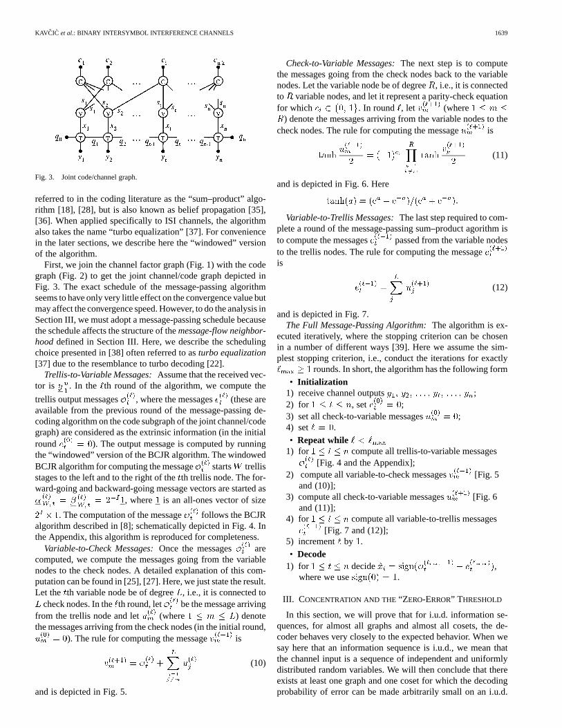
1642 IEEE TRANSACTIONS ON INFORMATION THEORY, VOL. 49, NO. 7, JULY 2003
erroneous after rounds of the message-passing decoding algo-rithm is highly concentrated around the value . To do that,we need the following result from [23]. Define as the prob-ability that a neighborhood of depthis not a tree when a codegraph is chosen uniformly at random from all possible graphswith degree polynomials and . In [23], it is shown that
neighborhood not a tree (18)
where is a constant independent of.3
B. Concentration Theorems
Theorem 1: Let be the transmitted codeword. Letbe the random variable that denotes the number of
erroneous variable-to-check messages afterrounds of themessage-passing decoding algorithm when the code graph ischosen uniformly at random from the ensemble of graphs withdegree polynomials and . Let be the number ofvariable-to-check edges in the graph. For an arbitrarily smallconstant , there exists a positive number, such that if
, then
(19)
Proof: The proof follows closely the proof of the concen-tration theorem for memoryless channels presented in [25]. Firstnote that
(20)
The random variable depends on the deterministicsequence and its probability space is the union of the en-semble of graphs with degree polynomials , , and theensemble of channel noise realizations (which uniquely definethe channel outputs sinceis known). Following [23], [25], weform a Doob edge-and-noise-revealing martingale and applyAzuma’s inequality [40] to get
(21)
where depends only on , , and .Next, we show that the second term on the right-hand side of
(20) equals by using inequality (18). Again, this is adoptedfrom [25], but adapted to a channel with ISI memory. We have
(22)
3Actually, in [23] this fact is shown for a bipartite graph, but the extension tojoint code/channel graphs of Fig. 3 is straightforward.
and
(23)
Combining (22) and (23), if , we get
(24)
Theorem 2: Let be a random sequence of i.u.d. binaryrandom variables (symbols) . Let bethe random variable that denotes the number of erroneous vari-able-to-check messages afterrounds of the message-passingdecoding algorithm when the code graph is chosen uniformly atrandom from the ensemble of graphs with degree polynomials
and , and when the transmitted sequence is. Letbe the number of variable-to-check edges in the graph. For anarbitrarily small constant , there exists a positive number
, such that if , then
(25)
Proof: Using Theorem 1, we have the following:
(26)
Next, recognize that if is an i.u.d. random sequence, all neigh-borhood types are equally probable, i.e., .Using this, we prove that

KAV CIC et al.: BINARY INTERSYMBOL INTERFERENCE CHANNELS 1643
Now form a Doob symbol-revealing martingale sequence
If we can show that
(27)
where is a constant dependent on , , and (but notdependent on ) then if we apply Azuma’s inequality [40], wewill have
(28)
Then, by combining (28) and (26), for , wewill get (25). So, all that needs to be shown is (27).
Consider two random variables and . Therandom vectors and have the following properties:1) the first symbols of and are deterministic and equal
; 2) The th symbol of is the randomvariable , while the th symbol of is fixed (non-random) ; 3) the remaining symbols and
are i.u.d. binary random vectors statistically independentof each other. Fixing the th symbol,can affect at most a constant number (call this number)of message-flow neighborhoods of depth. The constantdepends on , , and , but it does not depend on.Therefore, for any given neighborhood type, we have
(29)
Using the notation , we can verify that
Defining , and using (29), we get
(30)
Inequality (27) follows from (30).
Corollary 2.1: Let be any information block consisting ofbinary digits. Let be a code chosen uniformly
at random from the ensemble of Gallager coset
codes. Let be a random variable representing the numberof erroneous variable-to-check messages in roundof themessage-passing decoding algorithm on the joint channel/codegraph of the code . Then
(31)
Proof: If and are chosen independently and uniformlyat random, then the resulting codeword in (7) consists of i.u.d.binary symbols, and Theorem 2 applies directly.
C. “Zero-Error” Threshold
The term “zero-error” threshold is a slight abuse because thedecoding error can never be made equal to zero, but the concen-tration probability can be equal to zero in the limit as ,and hence the probability of decoding error can be made arbi-trarily small. As in [25], the “zero-error” noise standard devia-tion threshold is defined as
(32)
where the supremum in (32) is taken over all noise standarddeviations for which
(33)
Corollary 2.2: Let be an information block chosen uni-formly at random from binary sequences of length.There exists a code in the ensemble ofGallager coset codes, such that for any , the probabilityof error can be made arbitrarily low, i.e., if is the numberof erroneous variable-to-check messages in roundof themessage-passing decoding algorithm on the joint channel/codegraph of the code , then
(34)
Proof: Define an indicator random variable
if
otherwise.(35)
From Corollary 2.1, for , , and chosen uniformly atrandom we have . Since the expectedvalue is lower than , we conclude that there must existat least one graph and one coset-defining vectorsuch thatfor chosen uniformly at random we have
i.e., there exists a graph and a coset-defining vectorsuchthat for chosen uniformly at random
(36)
The assumption guarantees
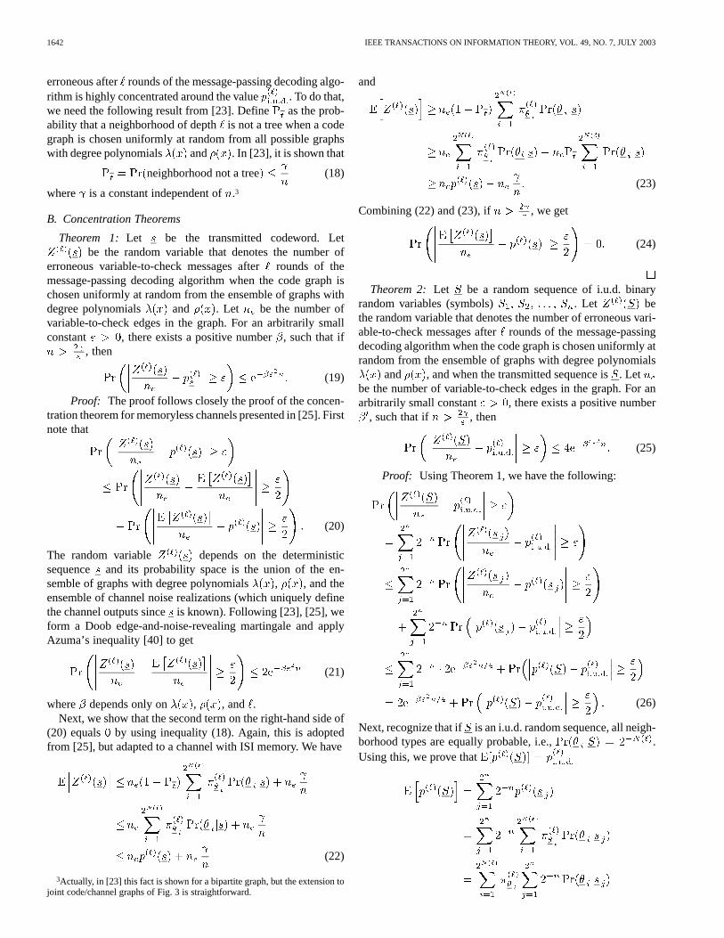
1644 IEEE TRANSACTIONS ON INFORMATION THEORY, VOL. 49, NO. 7, JULY 2003
Since , it follows that for every , thereexists an integer such that for every we have
. Then, for , we have
(37)
The desired result (34) follows by combining (36) and (37).
IV. DENSITY EVOLUTION AND THRESHOLDCOMPUTATION
A. Density Evolution
Define as the pdf of the message obtainedat the top of a depth-tree of type , see Fig. 8. With this no-tation, we may express the i.u.d. error concentration probabilityas
(38)
Here, is theaveragepdf (averaged over all tree types)of the correct message from a variable node to a check nodein round of the message-passing algorithm on a tree. We canobtain the pdf in several different ways. Here, we per-form the averaging in every round and enter a new round withan average pdf from the previous round, i.e., weevolveinto . This method was used in [14] for discrete mes-sages and in [25] for continuous messages, where it was termeddensity evolution.
Denote by theaveragedensity (pdf) of a messagein the th round of the message-passing algorithm (averagedover all tree types), see Fig. 5. Let denote theaveragepdf of a message in the th round of the message-passingalgorithm on a tree. Then the average density (pdf) isgiven by
(39)
where stands for the convolution operation, and de-notes the convolution of pdfs. As shorthand, we use thefollowing notation:
(40)
We also drop the function argumentsince it is common for allconvolved pdfs. Then (39) may be conveniently expressed as
(41)
Equation (41) denotes the evolution of the average density (pdf)through a variable node, Fig. 5.
To express the density evolution through a check node(Fig. 6), we require a variable change, resulting in a cumber-some change of measure. A convolution can then be defined inthe new domain and an expression can be found for the densityevolution through check nodes [25]. Here we do not pursue thisrather complicated procedure because a numerical method fordensity evolution through check nodes can easily be obtainedthrough a table lookup, for details see [27]. Here we simplydenote this density evolution as
(42)
where is symbolic notation for the average mes-sage density obtained by evolving the density througha check node of degree. We further express (42) by the fol-lowing notation:
(43)
Similar to (41), the average density (pdf) of messages(Fig. 7) is obtained using the convolution operator
(44)Note that in this equation the degree distribution is averagedwith respect to the nodes, rather than the edges. This explains theterm , which is the fraction of variable nodes
with degree . The notation is symbolic shorthand.The step that is needed to close the loop of a single densityevolution round is the evolution of the average densityinto the average density , i.e., the evolution of messagedensities through the trellis portion of the joint code/channelgraph. We denote this step as
(45)
where is symbolic notation fortrellis evolutionand de-notes the pdf of the channel noise (in this case a zero-meanGaussian with variance ). Even though no closed-form so-lution for (45) is known, it can be calculated numerically usingMonte Carlo techniques.
The density evolution is now given by
• Initialization1) ;
2) set (where is the Dirac function).• For to
1) ;
2) ;

KAV CIC et al.: BINARY INTERSYMBOL INTERFERENCE CHANNELS 1645
3) ;
4) .
• Compute1) .
B. Threshold Computation
With the density evolution algorithm described in the pre-vious subsection, the zero-error thresholdcan be evaluated(up to the numerical accuracy of the computation machine) asthe maximal value of the noise variancefor which ,where is the numerical accuracy tolerance.
With a finite-precision machine, we must quantize themessages, resulting in a discrete probability mass function.For a sufficiently large number of quantization levels, thediscrete probability mass functions are good approximations ofcontinuous density functions (pdfs) , , , and . Inthe for-loop of the density evolution algorithm in Section IV-A,steps 2) and 4) are straightforward convolutions (easily im-plemented numerically using the fast Fourier transform [41]).Step 1) of the for-loop can easily be implemented using a tablelookup as explained in [27], or using a rather cumbersomechange of measure explained in [25]. Actually, only step 3) ofthe for-loop needs further explanation. Since no closed-formsolution is known for evolving densities through trellis sections,we employ aMonte Carloapproach to obtain a histogram thatclosely approximates . This has first been suggested in [26]for trellises of constituent convolutional codes of turbo codes.In [26], Richardson and Urbanke run the BCJR algorithm ona long trellis section when the input is the all-zero sequence.Here, since the channel has memory, the transmitted sequencemust be a randomly chosen i.u.d. binary sequence. The length
of the sequence must be very long so that we can ignore thetrellis boundary effects.
To implement step 3) of the for-loop in the density evolu-tion algorithm in Section IV-A, for we generate thesymbols independently and uniformly at random.They are then transmitted over the noisy ISI channel to get thechannel output realization . We generate the extrinsic infor-
mation for as follows. For all , firstcreate independent realizations according to the pdf (actu-ally, histogram) , and then set . For ,we compute thea priori probability that the message symbolequals as
Using these prior probabilities and using as the channeloutputs, we run the BCJR algorithm [8] to compute the trellisoutputs . We then equate to the histogram of thevalues , where , and is chosenlarge enough to avoid the trellis boundary effects. In [26], thistechnique is accelerated by forcing the consistency condition onthe histogram. In ISI channels, however, consistency generallydoes not hold, so we must use a larger trellis section in theMonte Carlo simulation.
V. ACHIEVABLE RATES OFGALLAGER CODES
A. Achievable Rates of Binary Linear Codes Over ISIChannels
In Section II, we pointed out that is the limit (as) of the average mutual information between and
when is an i.i.d. sequence with
Since the input process, the channel, and, hence, the outputprocess and the joint input–output process are all stationary andergodic, one can adopt the standard random coding technique[1] to prove a coding theorem to assure that all ratesareachievable(for the definition ofachievable, see [2, p. 194]).We use the expression “standard random coding technique” todescribe a method to generate the codebook, where codewordsare chosen independently at random and the coded symbols aregoverned by the optimal input distribution. For a generic fi-nite-state channel, see [1, Sec. 5.9] or [42] for a detailed descrip-tion of the problem and the the proof of the coding theorem. Forthe channel in (1) with binary inputs, we present a somewhatstronger result involvinglinear codes.4
Theorem 3: Every rate is achievable; further-more, the rate can be achieved by linear block codes or theircoset codes.
Proof: From [5], if the channel input is an i.u.d.(Bernoulli-1/2) sequence, we have
where the second equality follows from the fact that the channelin (1) can be driven into any known state, with at mostinputs (where is the ISI length). For any , there exists apositive integer such that and
where the starting state is a known vector of binary values,say . Now we consider the followingtransmission scheme. We transmit a binary vector, where be-fore every block of symbols we transmit the known sequence
, i.e.,
...
(46)
Clearly, from (46), for any , we have
and
4Here we use a different (and apparently simpler) proof methodology. How-ever, the proof only applies to finite-state channels for which we can guaranteethat we can achieve any state with a finite number of channel inputs (e.g., ISIchannels with finite ISI memory); not for a general finite-state channel.

1646 IEEE TRANSACTIONS ON INFORMATION THEORY, VOL. 49, NO. 7, JULY 2003
The symbols of the vector are transmitted over the channelin (1) to obtain a vector at the channel output. Similar to thevector in (46), we partition the vector as
...
where for any any , we have
and
Clearly, we have a memoryless vector-channel as follows:Input: whose realization is a binary vector
Output: whose realization is real vector .The probability law of the vector channel is defined by the
following conditional pdf:
since the known sequence is transmitted before every vector. This channel transition probability law is well defined [1],
[42], hence, ; is also well defined. Note that thepdf is not dependent on, which makes it possible tofactor the joint pdf as
showing that the vector channel is indeed memoryless. Further,quantize the output vector to get a quantized vector
. Due to [1, Ch. 7], we can always find a quantizerto get a discrete channel such that the corresponding averagemutual information ; is greater than the givenrate . Since is arbitrarily small, we can choose integersand
such that
Similar to [2, proof of Theorem 8.7.1, p. 198], we can provethat is achievable for the obtained discrete memorylesschannel. The reader should note that the random code wegenerated has codewords, which are statistically inde-pendent. The coded symbols are i.u.d., each with probability
. Every codeword consists of vector symbols from, say . The transmitted block
is with length . So,
the real code rate is . The received sequence also has thesame block length. However, from [2, proof of Theorem 8.7.1,p. 198], the decoding error probability can be made arbitrarilysmall even if we only use the typical-set decoding with respectto and , which is not the full received sequence.
To prove the second part of this theorem, we should notethat the error probability bound only depends on the statisticalproperties of the random codebook. We can generate a code-book by drawing codewords uniformly at random as in [1, The-orem 6.2.1, p. 206].
For binary ISI channels, define the capacity as thesupremum of rates achievable by binary linear codes underany decoding algorithm. A consequence of Theorem 3 is
(47)
Formulating the exact relationship between , , ,and is still an open problem since to the best of our knowledgeneither the literature nor the theorems presented in this paperanswer this question. For example, it is our belief that the strictinequality must hold because binary linear codescannot achieve spectral shaping required to match the spectralnulls of the code to the spectral nulls of the channel (see [43]for matched spectral null codes), but we cannot back up thisstatement with a proof. Further, we know (at least for some ISIchannels) that . An example can be constructedby concatenating an outer regular rate-Gallager code whosevariable node degree is and check node degreeis , with an inner matched spectral null biphasecode [43] of rate . For this special construction, the resultingcode is a linear (coset) code of rate–. If we use this code fortransmission over the dicode channel ( channel), thoughnot explicitly shown here, we can compute that the zero-errorthreshold of message-passing decoding is above (wherefor this channel it can be numerically shown using the algorithmin [9], [10] that ).
While the exact relationship between , , and isstill an open problem, we can prove a relationship between thezero-error threshold of the message-passing decoder of Gallagercodes, and the values and .
Proposition 1: Let be the rate of a Gallager code and letbe the threshold computed by density evolution using i.u.d.
inputs. Then , where and areevaluated at the noise standard deviation .
Proof: According to the concentration theorem, theaverage probability of error (averaged over all random choicesof the graph, the coset vector, and the information-bearingvector ) can be made arbitrarily small if . Thatmeans that there exists at least one graph that achieves anarbitrarily small average probability of decoding error (aver-aged over all random choices of the coset vectorand theinformation-bearing vector ). Pick the parity-check matrixcorresponding to this graph as our code matrix. We design thefollowing transmission scheme. The messagesare chosenuniformly at random and the coset vectorsare chosen alsouniformly at random. The resulting transmitted sequence isi.i.d. with probability of each symbol , that is, the sequenceis i.u.d. If the transmitted sequence is i.u.d., we cannot find a
KAV CIC et al.: BINARY INTERSYMBOL INTERFERENCE CHANNELS 1647
code with rate higher than such that the decoding erroris arbitrarily small. But since the decoding error (averaged overall messages and all cosets ) for the sum–product decoderof Gallager codes can be made arbitrarily small for , weconclude that the code ratemust be smaller than the value for
evaluated at . Therefore,
B. Thresholds for Regular Gallager Codes as Lower Boundson
The two proofs presented in the preceding subsectionestablish that the curve rate versus threshold for aGallager code over a binary ISI channel is upper-boundedby the curve versus , and upper-bounded by thecurve versus . Thus, we have a practical method fornumerically lower-bounding . Furthermore, by virtueof specifying the degree polynomials and , we alsocharacterize a code that can achieve this lower bound. Thisis a bounding method that is different from the closed-formbounds [6], [7] or Monte Carlo bounds [5] proposed in thepast, where no bound-achieving characterization of the codeis possible (except through random coding techniques whichare impractical for implementations). Further, we compare thethresholds obtained by density evolution to the valuecomputed by the Arnold–Loeliger method [9], showing thatthe thresholds are very close to in the high-code-rateregions . This is exactly the region of practicalimportance in storage devices where high-rate codes for binaryISI channels are a necessity [3]. The codes studied in this paperdo not provide tight bounds in the low-rate region, but thethreshold bounds can be tightened by optimizing the degreepolynomials and , see [44].
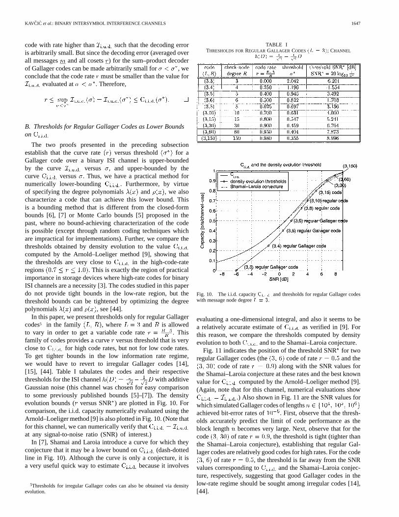
In this paper, we present thresholds only for regular Gallagercodes5 in the family , where and is allowedto vary in order to get a variable code rate . Thisfamily of codes provides a curveversus threshold that is veryclose to for high code rates, but not for low code rates.To get tighter bounds in the low information rate regime,we would have to revert to irregular Gallager codes [14],[15], [44]. Table I tabulates the codes and their respectivethresholds for the ISI channel with additiveGaussian noise (this channel was chosen for easy comparisonto some previously published bounds [5]–[7]). The densityevolution bounds ( versus SNR) are plotted in Fig. 10. Forcomparison, the i.i.d. capacity numerically evaluated using theArnold–Loeliger method [9] is also plotted in Fig. 10. (Note thatfor this channel, we can numerically verify thatat any signal-to-noise ratio (SNR) of interest.)
In [7], Shamai and Laroia introduce a curve for which theyconjecture that it may be a lower bound on (dash-dottedline in Fig. 10). Although the curve is only a conjecture, it isa very useful quick way to estimate because it involves
5Thresholds for irregular Gallager codes can also be obtained via densityevolution.
TABLE ITHRESHOLDS FORREGULAR GALLAGER CODES (L = 3); CHANNEL
h(D) = � D
Fig. 10. The i.i.d. capacityC and thresholds for regular Gallager codeswith message node degreeL = 3.
evaluating a one-dimensional integral, and also it seems to bea relatively accurate estimate of as verified in [9]. Forthis reason, we compare the thresholds computed by densityevolution to both and to the Shamai–Laroia conjecture.
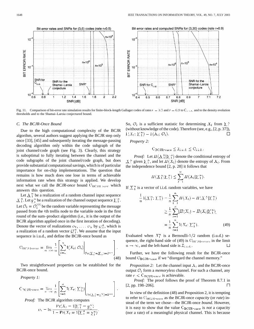
Fig. 11 indicates the position of the threshold SNRfor tworegular Gallager codes (the code of rate and the
code of rate ) along with the SNR values forthe Shamai–Laroia conjecture at these rates and the best knownvalue for computed by the Arnold–Loeliger method [9].(Again, note that for this channel, numerical evaluations show
.) Also shown in Fig. 11 are the SNR values forwhich simulated Gallager codes of lengthsachieved bit-error rates of . First, observe that the thresh-olds accurately predict the limit of code performance as theblock length becomes very large. Next, observe that for thecode of rate , the threshold is tight (tighter thanthe Shamai–Laroia conjecture), establishing that regular Gal-lager codes are relatively good codes for high rates. For the code
of rate , the threshold is far away from the SNRvalues corresponding to and the Shamai–Laroia conjec-ture, respectively, suggesting that good Gallager codes in thelow-rate regime should be sought among irregular codes [14],[44].
1648 IEEE TRANSACTIONS ON INFORMATION THEORY, VOL. 49, NO. 7, JULY 2003
Fig. 11. Comparison of bit-error rate simulation results for finite-block-length Gallager codes of ratesr = 0:5 andr = 0:9 toC and to the density evolutionthresholds and to the Shamai–Laroia conjectured bound.
C. The BCJR-Once Bound
Due to the high computational complexity of the BCJRalgorihm, several authors suggest applying the BCJR step onlyonce [33], [45] and subsequently iterating the message-passingdecoding algorithm only within the code subgraph of thejoint channel/code graph (see Fig. 3). Clearly, this strategyis suboptimal to fully iterating between the channel and thecode subgraphs of the joint channel/code graph, but doesprovide substantial computational savings, which is of particularimportance for on-chip implementations. The question thatremains is how much does one lose in terms of achievableinformation rate when this strategy is applied. We developnext what we call theBCJR-oncebound whichanswers this question.
Let be a realization of a random channel input sequence. Let be a realization of the channel output sequence.
Let be the random variable representing the messagepassed from theth trellis node to the variable node in the firstround of the sum–product algorithm (i.e., it is the output of theBCJR algorithm applied once in the first iteration of decoding).Denote the vector of realizations by , which isa realization of a random vector . We assume that the inputsequence is i.u.d., and define the BCJR-once bound as
-
(48)
Two straightforward properties can be established for theBCJR-once bound.
Property 1:
-
Proof: The BCJR algorithm computes
So, is a sufficient statistic for determining from(without knowledge of the code). Therefore (see, e.g., [2, p. 37]),
.
Property 2:
-
Proof: Let denote the conditional entropy ofgiven , and let denote the entropy of . From
the independence bound [2, p. 28] it follows that
If is a vector of i.i.d. random variables, we have
(49)
Evaluated when is a Bernoulli- random (i.u.d.) se-quence, the right-hand side of (49) is - , in the limit
, and the left-hand side is .
Further, we have the following result for the BCJR-oncebound - if we “disregard the channel memory.”
Proposition 2: Let the channel input and the BCJR-onceoutput form amemorylesschannel. For such a channel, anyrate - is achievable.
Proof: The proof follows the proof of Theorem 8.7.1 in[2, pp. 198–206].
In view of the definition (48) and Proposition 2, it is temptingto refer to - as the BCJR-oncecapacity(or rate) in-stead of the term we chose—the BCJR-oncebound. However,it is easy to show that the value - is not a capacity(nor a rate) of a meaningful physical channel. This is because
KAV CIC et al.: BINARY INTERSYMBOL INTERFERENCE CHANNELS 1649
the physical channel is not memoryless as assumedin Proposition 2, and we have
-
On the other hand, we believe it is appropriate to refer to- as a bound because in Section V-D we show
that the rate achievable by message-passing decoding ofrandomly constructed Gallager (coset) codes is upper-boundedby - .
The BCJR-once bound - for the channel in (1)can be computed by i) running the BCJR algorithm on a verylong trellis section, ii) collecting the outputs, iii) quantizingthem, iv) forming a histogram for the symbol-to-symbol tran-sition probabilities, and v) computing the mutual informationof a memoryless channel whose transition probabilities equalthose computed by the histogram. Another way is to devise amethod similar to the Arnold–Loeliger method for computing
(see [9]). First, we note that for i.u.d. input symbols,. Thus, the problem of computing -
reduces to the problem of computing
(50)
where is the binary entropy function defined as. For a given channel output
realization , the BCJR algorithm computes .So, we can estimate (50) by generating an-long i.u.d. inputsequence, transmitting it over the channel and running the BCJRalgorithm on the observed channel output to get
for every . The estimate
-
converges with probability to - as .The BCJR-once bound - (computed in the manner
described above for ) is depicted as the dashed curvein Fig. 12 (the same figure also shows three other curves:1) the curve for as computed by the Arnold-Loeligermethod, 2) the thresholds presented in Section V-B, and 3) theBCJR-once thresholds for regular Gallager codes which arepresented next in Section V-D).
D. BCJR-Once Thresholds for Gallager Codes
Just as we performed density evolution for the fullsum–product algorithm over the joint channel/code graph,we do the same for theBCJR-onceversion of the decodingalgorithm. The only difference here is in the shape of thedepth- message flow neighborhood, while the general methodremains the same. Denote by - the noise toler-ance threshold for the BCJR-once sum–product algorithmfor a Gallager-code/ISI-channel combination. The threshold
- can be computed by density evolution on a tree-likemessage-flow neighborhood assuming that the trellis portion
of the sum–product algorithm is executed only in the firstdecoding round.
Proposition 3: Let be the rate of a Gallager code andlet - be the BCJR-once noise tolerance threshold(computed by density evolution using i.u.d. inputs). Then
- , where - is the BCJR-once boundevaluated at the noise standard deviation - .
Proof: The threshold - is computed using thedensity evolution method described in Section IV-A, where thetrellis evolution step is executed only in the first round. Thus, thethreshold - is computed as the threshold of a Gallagercode of rate on a memoryless channel, whose channel law(conditional pdf of channel output given the channel input) isgiven by
Here is the output of the windowed BCJR algorithm whenthe window size is , and clearly, due to the channel symmetry
As evident from the density averaging in the trellis portion ofthe density evolution, the function is the
average conditional pdf of , taken over all conditional pdfsof conditioned on under the constraint ,i.e.,
For this channel, when the noise standard deviation is, thechannel information rate is , where
. Similar to the proof of Proposition1, we use a Gallager code where the coset vector is chosenuniformly at random in each block transmission. For thisGallager code of rate, the transmitted symbols are i.u.d. Fromthe concentration theorem, we have that if - ,then the probability of decoding error is arbitrarily small. Sincethe probability of error can be made arbitrarily small,mustsatisfy - . Now, let , and we get
- - -
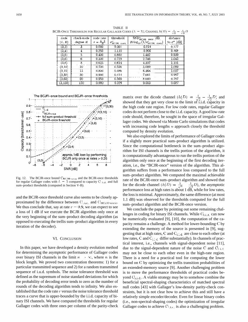
Again, we choose the family of regular Gallager codes with aconstant variable node degree and a varying check nodedegree . The channel is with AWGN.The BCJR-once thresholds are given in Table II, and the corre-sponding plot is given in Fig. 12. Fig. 12 shows the BCJR-oncebound derived in Section V-C. It can be seen that the regularGallager codes have the capability to achieve the BCJR-oncebound at high information rates if the BCJR-once version ofthe message-passing decoding algorithm is applied. For com-parison, Fig. 12 also shows the curve for as computedby the Arnold–Loeliger method [9]. (It can be numerically ver-ified for this channel that .) The figure showsthat the BCJR-once bound is very close to at low SNRs,but is about 1 dB away from at higher information rates.The difference between the full sum–product threshold curve
1650 IEEE TRANSACTIONS ON INFORMATION THEORY, VOL. 49, NO. 7, JULY 2003
TABLE IIBCJR-ONCE THRESHOLDS FORREGULAR GALLAGER CODES(L = 3); CHANNEL h(D) = � D
Fig. 12. The BCJR-once boundC - and the BCJR-once thresholdsfor regular Gallager codes withL = 3 compared to capacityC and fullsum–product thresholds (computed in Section V-B).
and the BCJR-once threshold curve also seems to be closely ap-proximated by the difference between and - .We thus conclude that, say at rate , we can expect to seea loss of 1 dB if we execute the BCJR algorithm only once atthe very beginning of the sum–product decoding algorithm (asopposed to executing the trellis sum–product algorithm in everyiteration of the decoder).
VI. CONCLUSION
In this paper, we have developed a density evolution methodfor determining the asymptotic performance of Gallager codesover binary ISI channels in the limit , where is theblock length. We proved two concentration theorems: 1) for aparticular transmitted sequence and 2) for a random transmittedsequence of i.u.d. symbols. The noise tolerance threshold wasdefined as the supremum of noise standard deviations for whichthe probability of decoding error tends to zero as the number ofrounds of the decoding algorithm tends to infinity. We also es-tablished that the code rateversus the noise tolerance thresholdtraces a curve that is upper-bounded by the i.i.d. capacity of bi-nary ISI channels. We have computed the thresholds for regularGallager codes with three ones per column of the parity-check
matrix over the dicode channel andshowed that they get very close to the limit of i.i.d. capacity inthe high code rate region. For low code rates, regular Gallagercodes do not perform close to the i.i.d. capacity. A good low-ratecode should, therefore, be sought in the space of irregular Gal-lager codes. We showed via Monte Carlo simulations that codeswith increasing code lengths approach closely the thresholdcomputed by density evolution.
We also explored the limits of performance of Gallager codesif a slightly more practical sum–product algorithm is utilized.Since the computational bottleneck in the sum–product algo-rithm for ISI channels is the trellis portion of the algorithm, itis computationally advantageous to run the trellis portion of thealgorithm only once at the beginning of the first decoding iter-ation, i.e., the “BCJR-once” version of the algorithm. This al-gorithm suffers from a performance loss compared to the fullsum–product algorithm. We computed the maximal achievablerate of the BCJR-once sum–product algorithm and showed thatfor the dicode channel , the asymptoticperformance loss at high rates is about 1 dB, while for low rates,the loss is minimal. Approximately, the same difference (at most1.1 dB) was observed for the thresholds computed for the fullsum–product algorithm and the BCJR-once version.
We conclude the paper by pointing out some remaining chal-lenges in coding for binary ISI channels. While can nowbe numerically evaluated [9], [10], the computation of the ca-pacity remains a challenge. A method for lower-boundingbyextending the memory of the source is presented in [9], sug-gesting that at high rates,and are close to each other (atlow rates, and differ substantially). In channels of prac-tical interest, i.e., channels with signal-dependent noise [11],due to the signal-dependent nature of the noiseandmay not be close to each other even in the high-rate region.There is a need for a practical tool for computing the lowerbound on by optimizing the trellis transition probabilities ofan extended-memory source [9]. Another challenging problemis to move the performance thresholds of practical codes be-yond . A viable strategy may be to somehow combine thebeneficial spectral-shaping characteristics of matched spectralnull codes [43] with Gallager’s low-density parity-check con-straints, but it is not clear how to achieve this and still have arelatively simple encoder/decoder. Even for linear binary codes(i.e., non-spectral-shaping codes) the optimization of irregularGallager codes to achieve is also a challenging problem.
KAV CIC et al.: BINARY INTERSYMBOL INTERFERENCE CHANNELS 1651
APPENDIX
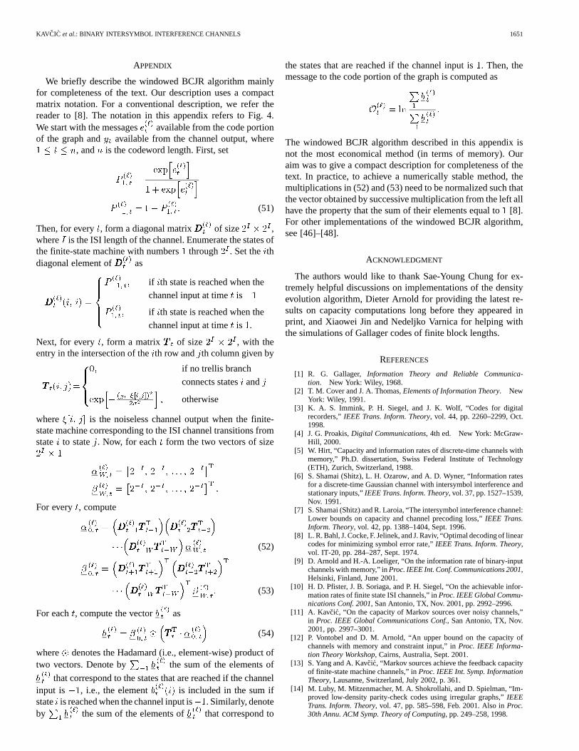
We briefly describe the windowed BCJR algorithm mainlyfor completeness of the text. Our description uses a compactmatrix notation. For a conventional description, we refer thereader to [8]. The notation in this appendix refers to Fig. 4.We start with the messages available from the code portionof the graph and available from the channel output, where
, and is the codeword length. First, set
(51)
Then, for every , form a diagonal matrix of size ,where is the ISI length of the channel. Enumerate the states ofthe finite-state machine with numbersthrough . Set the thdiagonal element of as
if th state is reached when the
channel input at time is
if th state is reached when the
channel input at time is .
Next, for every , form a matrix of size , with theentry in the intersection of theth row and th column given by
if no trellis branch
connects statesand
otherwise
where is the noiseless channel output when the finite-state machine corresponding to the ISI channel transitions fromstate to state . Now, for each form the two vectors of size
For every , compute
(52)
(53)
For each , compute the vector as
(54)
where denotes the Hadamard (i.e., element-wise) product oftwo vectors. Denote by the sum of the elements of
that correspond to the states that are reached if the channelinput is , i.e., the element is included in the sum ifstate is reached when the channel input is. Similarly, denoteby the sum of the elements of that correspond to
the states that are reached if the channel input is. Then, themessage to the code portion of the graph is computed as
The windowed BCJR algorithm described in this appendix isnot the most economical method (in terms of memory). Ouraim was to give a compact description for completeness of thetext. In practice, to achieve a numerically stable method, themultiplications in (52) and (53) need to be normalized such thatthe vector obtained by successive multiplication from the left allhave the property that the sum of their elements equal to[8].For other implementations of the windowed BCJR algorithm,see [46]–[48].
ACKNOWLEDGMENT
The authors would like to thank Sae-Young Chung for ex-tremely helpful discussions on implementations of the densityevolution algorithm, Dieter Arnold for providing the latest re-sults on capacity computations long before they appeared inprint, and Xiaowei Jin and Nedeljko Varnica for helping withthe simulations of Gallager codes of finite block lengths.
REFERENCES
[1] R. G. Gallager, Information Theory and Reliable Communica-tion. New York: Wiley, 1968.
[2] T. M. Cover and J. A. Thomas,Elements of Information Theory. NewYork: Wiley, 1991.
[3] K. A. S. Immink, P. H. Siegel, and J. K. Wolf, “Codes for digitalrecorders,”IEEE Trans. Inform. Theory, vol. 44, pp. 2260–2299, Oct.1998.
[4] J. G. Proakis,Digital Communications, 4th ed. New York: McGraw-Hill, 2000.
[5] W. Hirt, “Capacity and information rates of discrete-time channels withmemory,” Ph.D. dissertation, Swiss Federal Institute of Technology(ETH), Zurich, Switzerland, 1988.
[6] S. Shamai (Shitz), L. H. Ozarow, and A. D. Wyner, “Information ratesfor a discrete-time Gaussian channel with intersymbol interference andstationary inputs,”IEEE Trans. Inform. Theory, vol. 37, pp. 1527–1539,Nov. 1991.
[7] S. Shamai (Shitz) and R. Laroia, “The intersymbol interference channel:Lower bounds on capacity and channel precoding loss,”IEEE Trans.Inform. Theory, vol. 42, pp. 1388–1404, Sept. 1996.
[8] L. R. Bahl, J. Cocke, F. Jelinek, and J. Raviv, “Optimal decoding of linearcodes for minimizing symbol error rate,”IEEE Trans. Inform. Theory,vol. IT-20, pp. 284–287, Sept. 1974.
[9] D. Arnold and H.-A. Loeliger, “On the information rate of binary-inputchannels with memory,” inProc. IEEE Int. Conf. Communications 2001,Helsinki, Finland, June 2001.
[10] H. D. Pfister, J. B. Soriaga, and P. H. Siegel, “On the achievable infor-mation rates of finite state ISI channels,” inProc. IEEE Global Commu-nications Conf. 2001, San Antonio, TX, Nov. 2001, pp. 2992–2996.
[11] A. Kavcic, “On the capacity of Markov sources over noisy channels,”in Proc. IEEE Global Communications Conf., San Antonio, TX, Nov.2001, pp. 2997–3001.
[12] P. Vontobel and D. M. Arnold, “An upper bound on the capacity ofchannels with memory and constraint input,” inProc. IEEE Informa-tion Theory Workshop, Cairns, Australia, Sept. 2001.
[13] S. Yang and A. Kavcic, “Markov sources achieve the feedback capacityof finite-state machine channels,” inProc. IEEE Int. Symp. InformationTheory, Lausanne, Switzerland, July 2002, p. 361.
[14] M. Luby, M. Mitzenmacher, M. A. Shokrollahi, and D. Spielman, “Im-proved low-density parity-check codes using irregular graphs,”IEEETrans. Inform. Theory, vol. 47, pp. 585–598, Feb. 2001. Also inProc.30th Annu. ACM Symp. Theory of Computing, pp. 249–258, 1998.

1652 IEEE TRANSACTIONS ON INFORMATION THEORY, VOL. 49, NO. 7, JULY 2003
[15] T. Richardson, A. Shokrollahi, and R. Urbanke, “Design of capacity-ap-proaching low-density parity-check codes,”IEEE Trans. Inform.Theory, vol. 47, pp. 619–637, Feb. 2001.
[16] R. G. Gallager,Low-Density Parity-Check Codes. Cambridge, MA:MIT Press, 1962.
[17] B. M. Tanner, “A recursive approach to low complexity codes,”IEEETrans. Inform. Theory, vol. IT-27, pp. 533–547, Sept. 1981.
[18] N. Wiberg, H.-A. Loeliger, and R. Kötter, “Codes and iterative decodingon general graphs,”Europ. Trans. Commun., vol. 6, pp. 513–526, Sept.1995.
[19] G. D. Forney, Jr., “Codes on graphs: Normal realizations,”IEEE Trans.Inform. Theory, vol. 47, pp. 520–548, Feb. 2001.
[20] D. J. C. MacKay and R. M. Neal, “Near Shannon limit performance oflow-density parity-check codes,”Electron. Lett., vol. 32, pp. 1645–1646,1996.
[21] D. J. C. MacKay, “Good error-correcting codes based on very sparsematrices,”IEEE Trans. Inform. Theory, vol. 45, pp. 399–431, Mar. 1999.
[22] C. Berrou, A. Glavieux, and P. Thitimajshima, “Near Shannon limiterror-correcting coding and decoding: Turbo-codes,” inProc. IEEEInt. Conf. Communications, Geneva, Switzerland, May 1993, pp.1064–1070.
[23] M. G. Luby, M. Mitzenmacher, M. A. Shokrollahi, and D. A. Spielman,“Improved low density parity check codes using irregular graphs and be-lief propagation,” inProc. IEEE Int. Symp. Information Theory, Cam-bridge, MA, Aug. 1998, p. 117.
[24] M. Luby, M. Mitzenmacher, and M. A. Shokrollahi, “Analysis ofrandom processes via and-or tree evaluation,” inProc. 9th Annu.ACM-SIAM Symp. Discrete Algorithms, 1998, pp. 364–373.
[25] T. Richardson and R. Urbanke, “The capacity of low-density paritycheck codes under message-passing decoding,”IEEE Trans. Inform.Theory, vol. 47, pp. 599–618, Feb. 2001.
[26] , “Thresholds for turbo codes,” inProc. IEEE Int. Symp. Informa-tion Theory, Sorrento, Italy, June 2000, p. 317.
[27] S.-Y. Chung, G. D. Forney, Jr., T. Richardson, and R. Urbanke, “Onthe design of low-density parity-check codes within 0.0045 dB of theShannon limit,”IEEE Commun. Lett., vol. 5, pp. 58–60, Feb. 2001.
[28] F. R. Kschischang, B. J. Frey, and H.-A. Loeliger, “Factor graphs andthe sum-product algorithm,”IEEE Trans. Inform. Theory, vol. 47, pp.498–519, Feb. 2001.
[29] G. D. Forney, Jr., “Maximum-likelihood sequence estimation of digitalsequences in the presence of intersymbol interference,”IEEE Trans. In-form. Theory, vol. IT-18, pp. 363–378, Mar. 1972.
[30] J. Hagenauer and P. Hoeher, “A Viterbi algorithm with soft-decision out-puts and its applications,” inProc. IEEE Global TelecommunicationsConf., Dallas, TX, Nov. 1989, pp. 1680–1686.
[31] Y. Li, B. Vucetic, and Y. Sato, “Optimum soft-output detection for chan-nels with intersymbol interference,”IEEE Trans. Inform. Theory, vol.41, pp. 704–713, May 1995.
[32] M. P. C. Fossorier, F. Burkert, S. Lin, and J. Hagenauer, “On the equiv-alence between SOVA and max-log-MAP decodings,”IEEE Commun.Lett., vol. 2, pp. 137–139, May 1998.
[33] Z.-N. Wu and J. M. Cioffi, “Low-complexity iterative decoding withdecision-aided equalization for magnetic recording channels,”IEEE J.Select. Areas Commun., vol. 19, pp. 699–708, Apr. 2001.
[34] M. Tüchler, R. Kötter, and A. Singer, “Iterative correction of ISI viaequalization and decoding with priors,” inProc. IEEE Int. Symp. Infor-mation Theory, Sorrento, Italy, June 2000, p. 100.
[35] J. Pearl,Probabilistic Reasoning and Intelligent Systems. San Mateo,CA: Morgan Kaufmann, 1988.
[36] R. J. McEliece, D. J. C. MacKay, and J.-F. Cheng, “Turbo decoding as aninstance of Pearl’s belief propagation algorithm,”IEEE J. Select. AreasCommun., vol. 16, pp. 140–152, Feb. 1998.
[37] J. Douillard, M. Jezequel, C. Berrou, A. Picart, P. Didier, andA. Glavieux, “Iterative correction of intersymbol interference:Turbo-equalization,”Europ. Trans. Commun., vol. 6, pp. 507–511,Sept. 1995.
[38] J. Fan, A. Friedmann, E. Kurtas, and S. McLaughlin, “Low density paritycheck codes for magnetic recording,” inProc. Allerton Conf. Commu-nications and Control, 1999.
[39] D. J. C. MacKay. Gallager codes—Recent results. [Online]. Available:http://wol.ra.phy.cam.ac.uk/.
[40] R. Motwani and P. Raghavan,Randomized Algorithms. Cambridge,U.K.: Cambridge Univ. Press, 1995.
[41] A. V. Oppenheim and R. W. Schafer,Discrete-Time Signal Pro-cessing. Englewoods Cliffs, NJ: Prentice-Hall, 1989.
[42] A. Lapidoth and E. I. Telatar, “The compound channel capacity of aclass of finite-state channels,”IEEE Trans. Inform. Theory, vol. 44, pp.973–983, May 1998.
[43] R. Karabed and P. H. Siegel, “Matched spectral-null codes for partialresponse channels,”IEEE Trans. Inform. Theory, vol. 37, pp. 818–855,May 1991.
[44] N. Varnica and A. Kavcic, “Optimized LDPC codes for partial responsechannels,” inProc. IEEE Int. Symp. Information Theory, Lausanne,Switzerland, July 2002, p. 197.
[45] T. Souvignier, A. Friedmann, M. Öberg, P. Siegel, R. E. Swanson, and J.K. Wolf, “Turbo codes for PR4: Parallel versus serial concatenation,” inProc. IEEE Int. Conf. Communications, Vancouver, BC, Canada, June1999, pp. 1638–1642.
[46] S. Benedetto, D. Divsalaar, G. Montorsi, and F. Pollaara, “Algorithmfor continuous decoding of turbo codes,”Electron. Lett., vol. 32, pp.314–315, Feb. 1996.
[47] A. Viterbi, “An intuitive justification and a simplified implementationof the MAP decoder for convolutional codes,”IEEE J. Select. AreasCommun., vol. 16, pp. 260–264, Feb. 1998.
[48] B. Bai, X. Ma, and X. Wang, “Novel algorithm for continuous decodingof turbo codes,” inIEE Proc. Commun., vol. 46, Oct. 1999, pp. 314–315.