11

Binary Image AnalysisBinary Image Analysis

Binary image analysis

• consists of a set of image analysis operations that are used to produce or process binary images, usually images of 0’s and 1’s.

0 represents the background 1 represents the foreground

000100100010000001111000100000010010001000

22

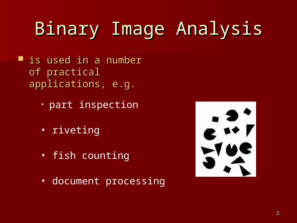
Binary Image AnalysisBinary Image Analysis

is used in a number of is used in a number of practical applications, practical applications, e.g.e.g.

• part inspection

• riveting

• fish counting

• document processing

33

What kinds of operations?What kinds of operations?

Separate objects from background and from one another

Aggregate pixels for each object

Compute features for each object

44

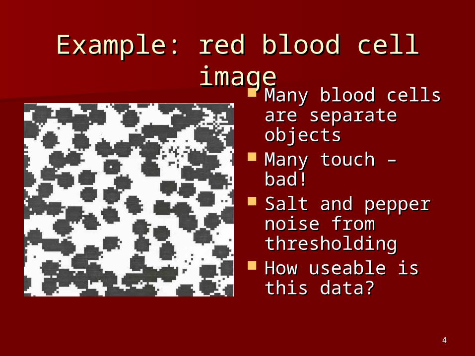
Example: red blood cell imageExample: red blood cell image Many blood cells Many blood cells

are separate are separate objectsobjects

Many touch – bad!Many touch – bad! Salt and pepper Salt and pepper

noise from noise from thresholdingthresholding

How useable is this How useable is this data?data?

55

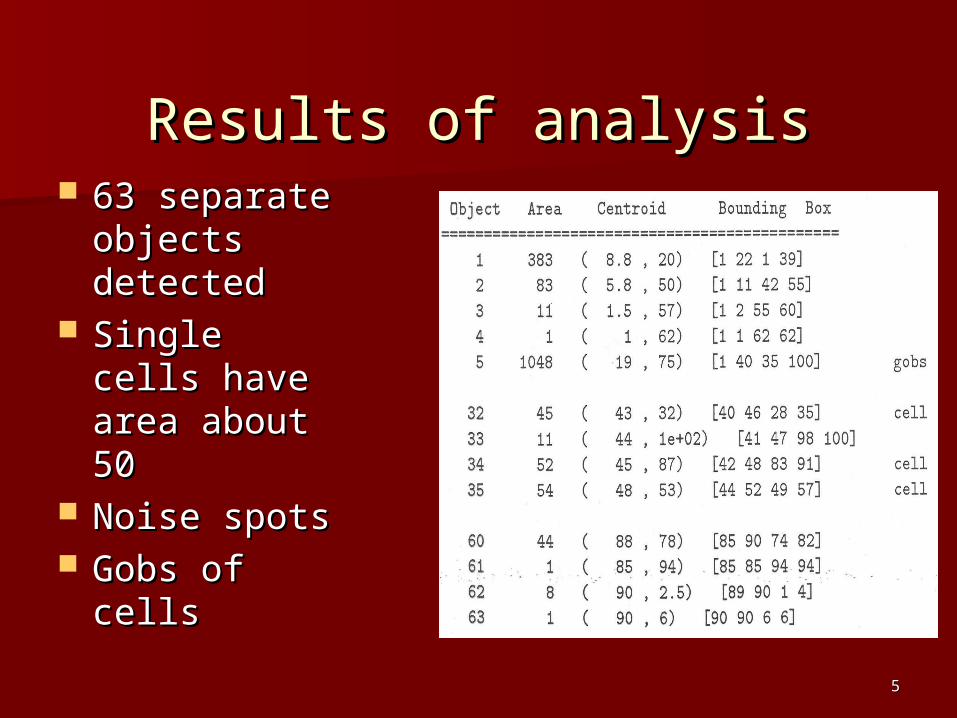
Results of analysisResults of analysis 63 separate 63 separate

objects objects detecteddetected

Single cells Single cells have area have area about 50about 50

Noise spotsNoise spots Gobs of cellsGobs of cells

66

Useful OperationsUseful Operations

1. Thresholding a gray-tone image

2. Determining good thresholds

3. Connected components analysis

4. Binary mathematical morphology

5. All sorts of feature extractors (area, centroid, circularity, …)

77

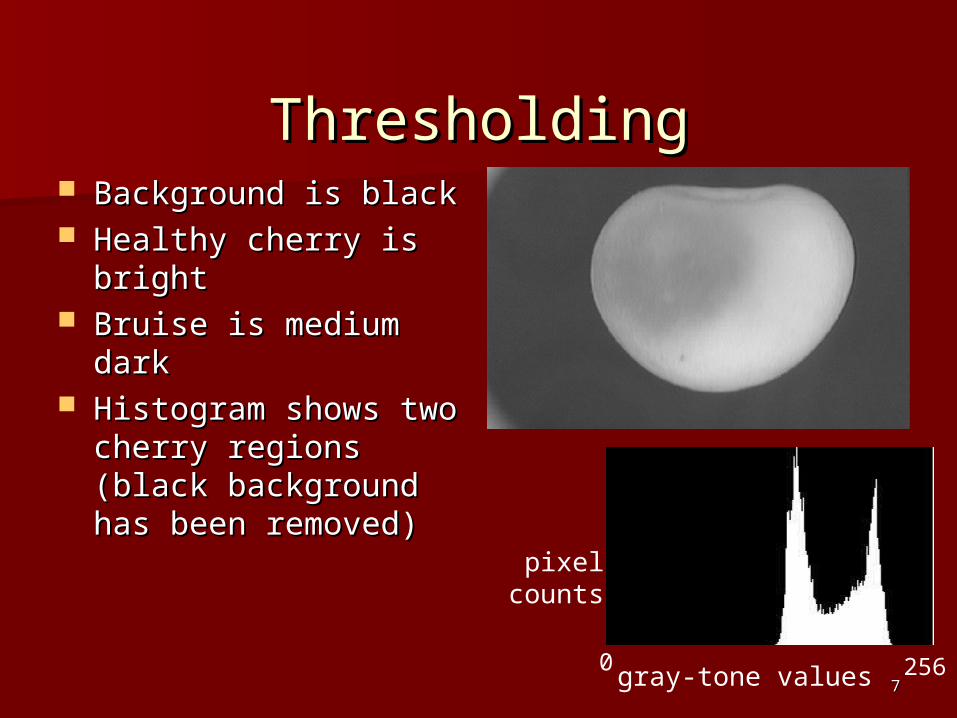
ThresholdingThresholding Background is blackBackground is black Healthy cherry is Healthy cherry is

brightbright Bruise is medium darkBruise is medium dark Histogram shows two Histogram shows two

cherry regions (black cherry regions (black background has been background has been removed)removed)

gray-tone values

pixelcounts

0 256

88

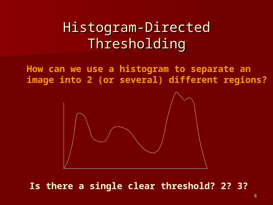
Histogram-Directed ThresholdingHistogram-Directed Thresholding

How can we use a histogram to separate animage into 2 (or several) different regions?

Is there a single clear threshold? 2? 3?

99

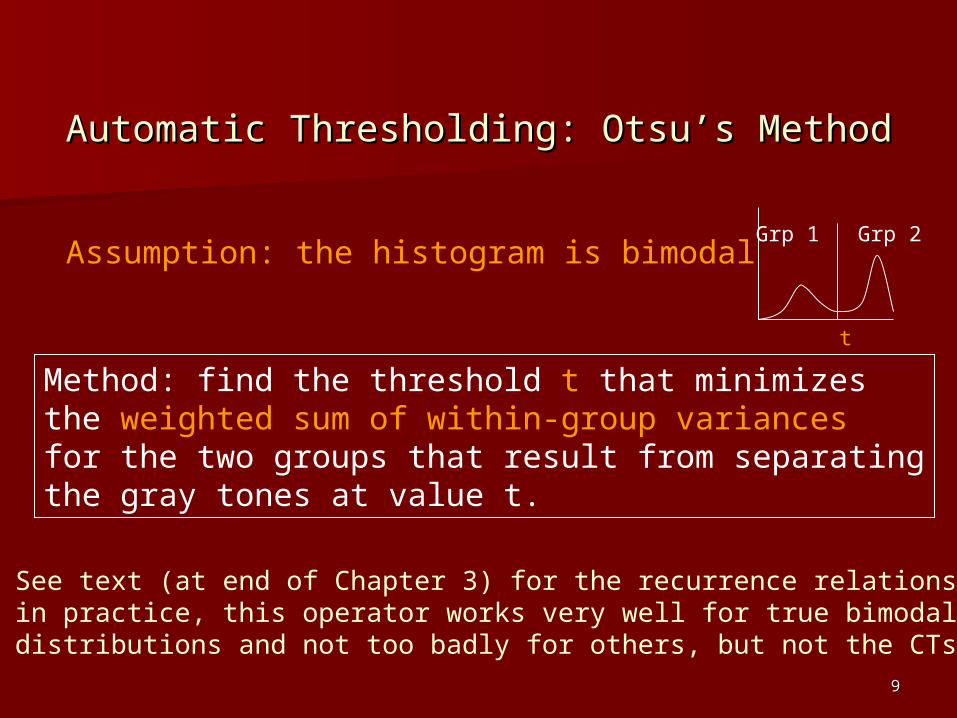
Automatic Thresholding: Otsu’s MethodAutomatic Thresholding: Otsu’s Method

Assumption: the histogram is bimodal

t

Method: find the threshold t that minimizesthe weighted sum of within-group variancesfor the two groups that result from separatingthe gray tones at value t.

See text (at end of Chapter 3) for the recurrence relations;in practice, this operator works very well for true bimodal distributions and not too badly for others, but not the CTs.

Grp 1 Grp 2

1010

Thresholding ExampleThresholding Example

original gray tone image binary thresholded image

1111

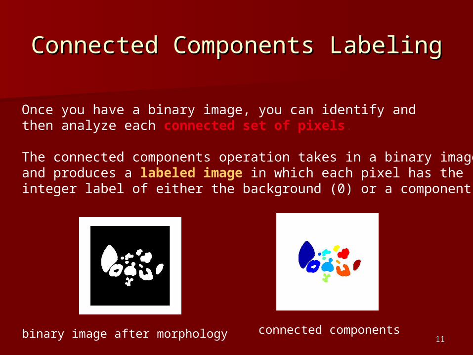
Connected Components LabelingConnected Components Labeling

Once you have a binary image, you can identify and then analyze each connected set of pixels.

The connected components operation takes in a binary image and produces a labeled image in which each pixel has the integer label of either the background (0) or a component.

binary image after morphology connected components

1212

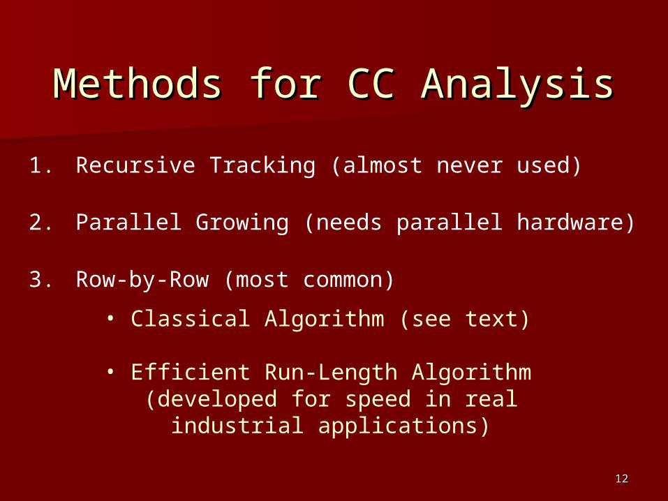
Methods for CC AnalysisMethods for CC Analysis

1. Recursive Tracking (almost never used)

2. Parallel Growing (needs parallel hardware)

3. Row-by-Row (most common)

• Classical Algorithm (see text)

• Efficient Run-Length Algorithm (developed for speed in real industrial applications)

1313

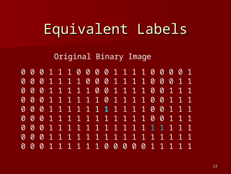
Equivalent LabelsEquivalent Labels

0 0 0 1 1 1 0 0 0 0 1 1 1 1 0 0 0 0 10 0 0 1 1 1 1 0 0 0 1 1 1 1 0 0 0 1 10 0 0 1 1 1 1 1 0 0 1 1 1 1 0 0 1 1 10 0 0 1 1 1 1 1 1 0 1 1 1 1 0 0 1 1 10 0 0 1 1 1 1 1 1 1 1 1 1 1 0 0 1 1 10 0 0 1 1 1 1 1 1 1 1 1 1 1 0 0 1 1 10 0 0 1 1 1 1 1 1 1 1 1 1 1 1 1 1 1 10 0 0 1 1 1 1 1 1 1 1 1 1 1 1 1 1 1 10 0 0 1 1 1 1 1 1 0 0 0 0 0 1 1 1 1 1

Original Binary Image

1414

Equivalent LabelsEquivalent Labels

0 0 0 1 1 1 0 0 0 0 2 2 2 2 0 0 0 0 30 0 0 1 1 1 1 0 0 0 2 2 2 2 0 0 0 3 30 0 0 1 1 1 1 1 0 0 2 2 2 2 0 0 3 3 30 0 0 1 1 1 1 1 1 0 2 2 2 2 0 0 3 3 30 0 0 1 1 1 1 1 1 1 1 1 1 1 0 0 3 3 30 0 0 1 1 1 1 1 1 1 1 1 1 1 0 0 3 3 30 0 0 1 1 1 1 1 1 1 1 1 1 1 1 1 1 1 10 0 0 1 1 1 1 1 1 1 1 1 1 1 1 1 1 1 10 0 0 1 1 1 1 1 1 0 0 0 0 0 1 1 1 1 1

The Labeling Process

1 21 3

1515

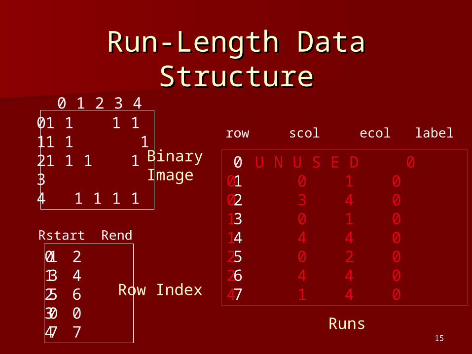
Run-Length Data StructureRun-Length Data Structure

1 1 1 11 1 11 1 1 1

1 1 1 1

0 1 2 3 401234

U N U S E D 00 0 1 00 3 4 01 0 1 01 4 4 02 0 2 02 4 4 04 1 4 0

row scol ecol label

01234567

Rstart Rend

1 23 45 60 07 7

01234 Runs

Row Index

BinaryImage

1616

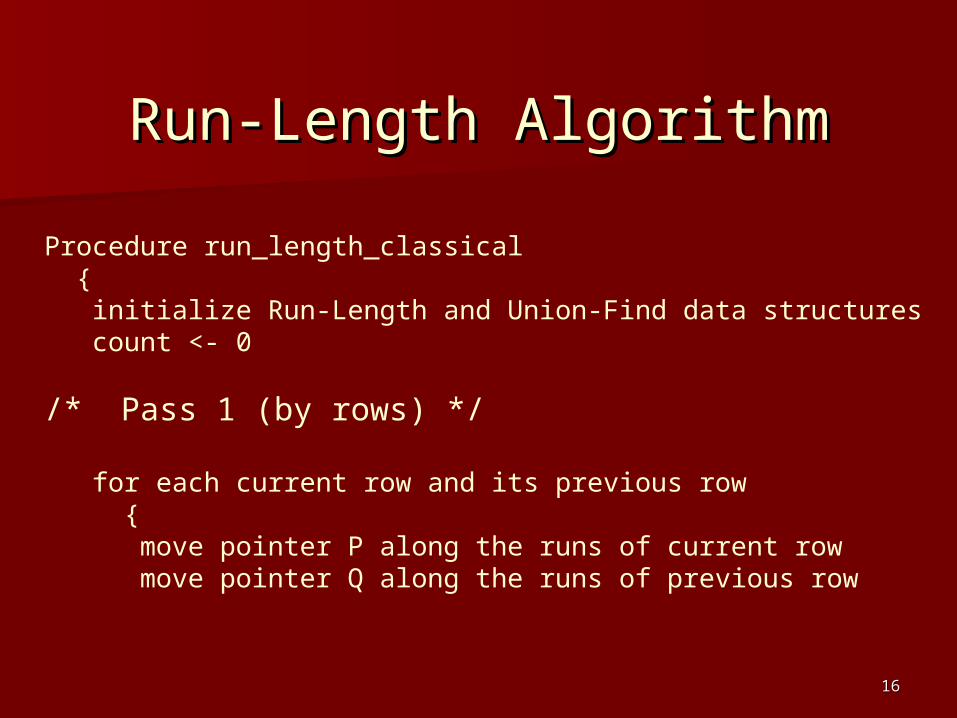
Run-Length AlgorithmRun-Length Algorithm

Procedure run_length_classical { initialize Run-Length and Union-Find data structures count <- 0

/* Pass 1 (by rows) */

for each current row and its previous row { move pointer P along the runs of current row move pointer Q along the runs of previous row

1717

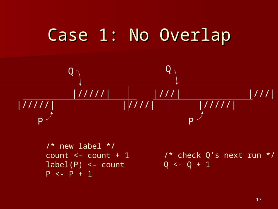
Case 1: No OverlapCase 1: No Overlap

|/////| |/////| |////|

|///| |///| |/////|

Q

P

Q

P

/* new label */ count <- count + 1 label(P) <- count P <- P + 1

/* check Q’s next run */Q <- Q + 1

1818

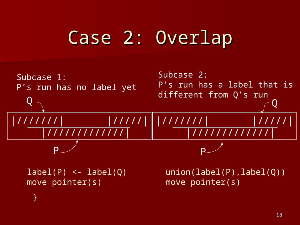
Case 2: OverlapCase 2: Overlap

Subcase 1: P’s run has no label yet

|///////| |/////| |/////////////|

Subcase 2:P’s run has a label that isdifferent from Q’s run

|///////| |/////| |/////////////|

QQ

P P

label(P) <- label(Q)move pointer(s)

union(label(P),label(Q))move pointer(s)

}

1919

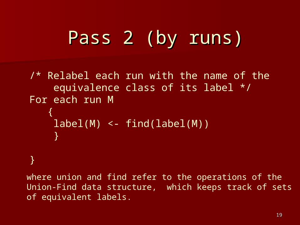
Pass 2 (by runs)Pass 2 (by runs)

/* Relabel each run with the name of the equivalence class of its label */For each run M { label(M) <- find(label(M)) }

}

where union and find refer to the operations of theUnion-Find data structure, which keeps track of setsof equivalent labels.

2020

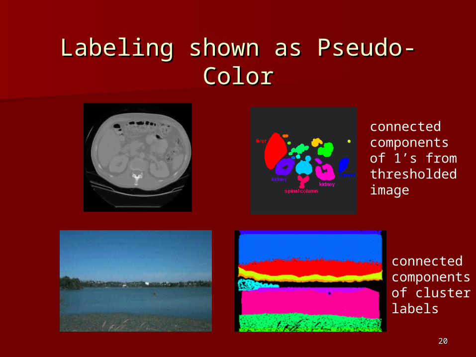
Labeling shown as Pseudo-ColorLabeling shown as Pseudo-Color

connectedcomponentsof 1’s fromthresholdedimage

connectedcomponentsof clusterlabels

2121

Mathematical MorphologyMathematical Morphology

Binary mathematical morphology consists of twobasic operations

dilation and erosion

and several composite relations

closing and opening conditional dilation . . .

2222

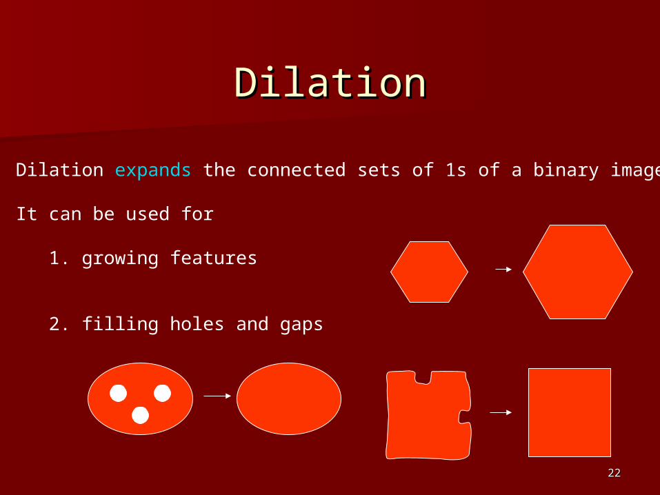
DilationDilation

Dilation expands the connected sets of 1s of a binary image.

It can be used for

1. growing features

2. filling holes and gaps

2323

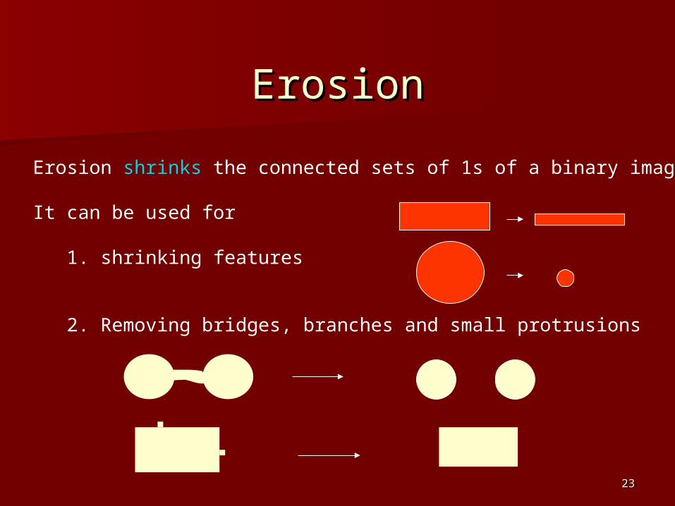
ErosionErosion

Erosion shrinks the connected sets of 1s of a binary image.

It can be used for

1. shrinking features

2. Removing bridges, branches and small protrusions

2424

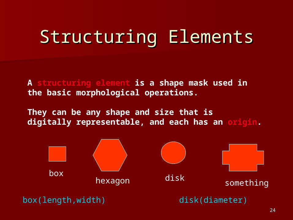
Structuring ElementsStructuring Elements

A structuring element is a shape mask used inthe basic morphological operations.

They can be any shape and size that isdigitally representable, and each has an origin.

boxhexagon disk

something

box(length,width) disk(diameter)

2525

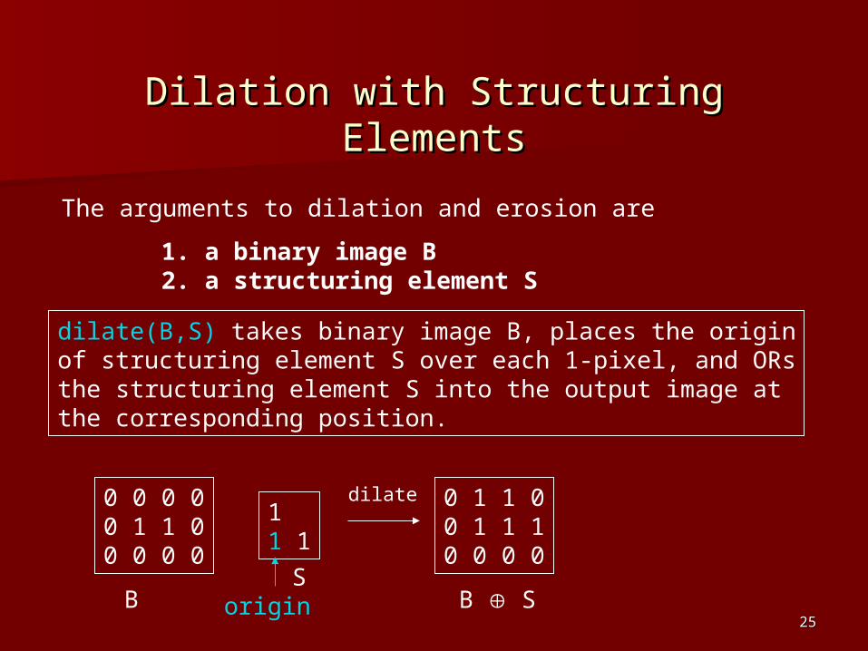
Dilation with Structuring ElementsDilation with Structuring Elements

The arguments to dilation and erosion are

1. a binary image B2. a structuring element S

dilate(B,S) takes binary image B, places the originof structuring element S over each 1-pixel, and ORsthe structuring element S into the output image atthe corresponding position.

0 0 0 00 1 1 00 0 0 0

11 1

0 1 1 00 1 1 10 0 0 0

originBS

dilate

B S

2626

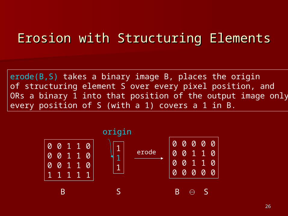
Erosion with Structuring ElementsErosion with Structuring Elements

erode(B,S) takes a binary image B, places the origin of structuring element S over every pixel position, andORs a binary 1 into that position of the output image only ifevery position of S (with a 1) covers a 1 in B.

0 0 1 1 00 0 1 1 00 0 1 1 01 1 1 1 1

111

0 0 0 0 00 0 1 1 00 0 1 1 00 0 0 0 0

B S

origin

erode

B S

2727

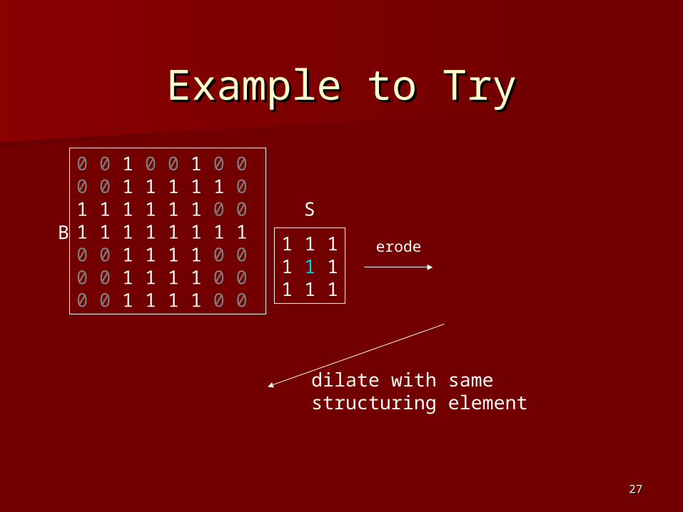
Example to TryExample to Try

0 0 1 0 0 1 0 0 0 0 1 1 1 1 1 0 1 1 1 1 1 1 0 01 1 1 1 1 1 1 10 0 1 1 1 1 0 0 0 0 1 1 1 1 0 0 0 0 1 1 1 1 0 0

1 1 11 1 11 1 1

erode

dilate with same structuring element

SB

2828

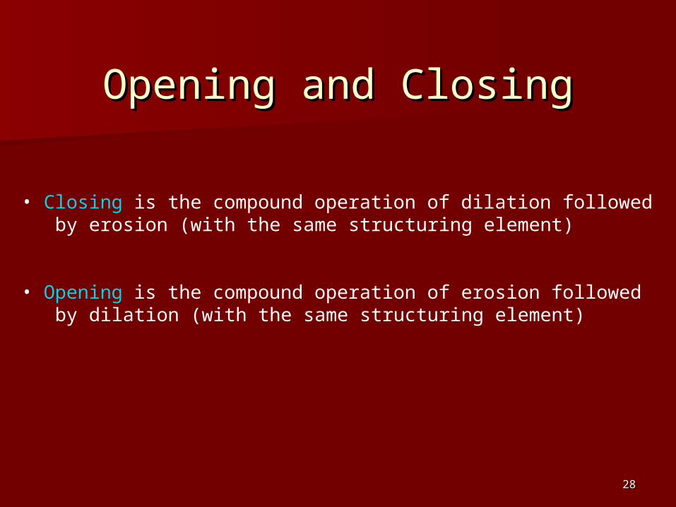
Opening and ClosingOpening and Closing

• Closing is the compound operation of dilation followed by erosion (with the same structuring element)

• Opening is the compound operation of erosion followed by dilation (with the same structuring element)

2929

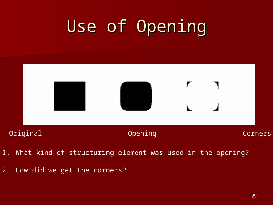
Use of OpeningUse of Opening

Original Opening Corners

1. What kind of structuring element was used in the opening?

2. How did we get the corners?

3030

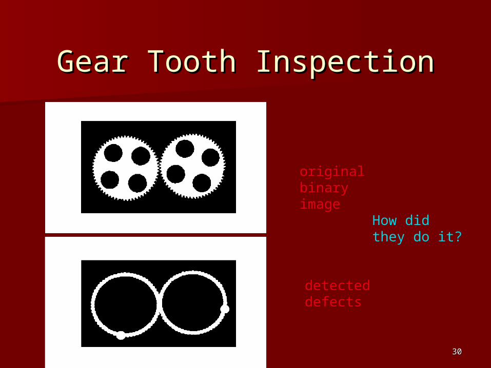
Gear Tooth InspectionGear Tooth Inspection

originalbinary image

detecteddefects

How didthey do it?

3131

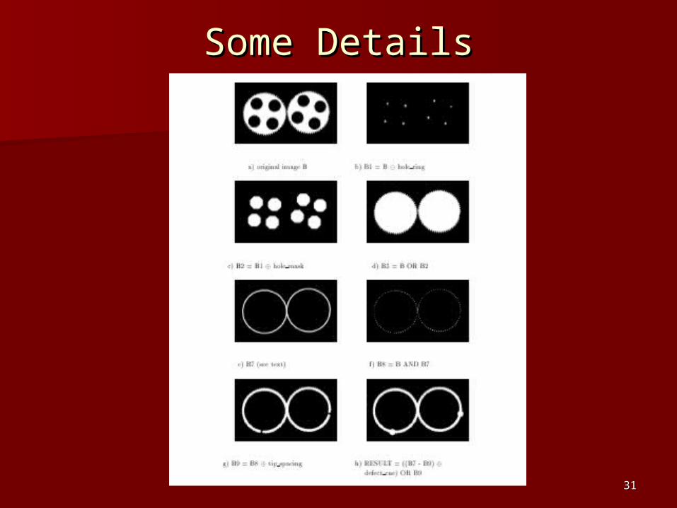
Some DetailsSome Details

3232

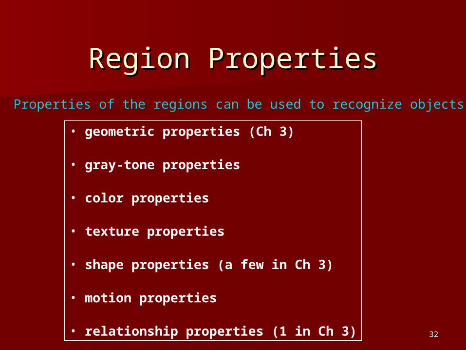
Region PropertiesRegion PropertiesProperties of the regions can be used to recognize objects.

• geometric properties (Ch 3)

• gray-tone properties

• color properties

• texture properties

• shape properties (a few in Ch 3)

• motion properties

• relationship properties (1 in Ch 3)

3333

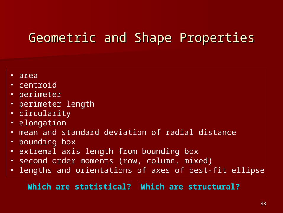
Geometric and Shape PropertiesGeometric and Shape Properties

• area• centroid• perimeter • perimeter length• circularity• elongation• mean and standard deviation of radial distance• bounding box• extremal axis length from bounding box• second order moments (row, column, mixed)• lengths and orientations of axes of best-fit ellipse

Which are statistical? Which are structural?

3434

Region Adjacency GraphRegion Adjacency Graph

A region adjacency graph (RAG) is a graph in whicheach node represents a region of the image and an edgeconnects two nodes if the regions are adjacent.

1

2

34

1 2

34