
Binary Decision Diagrams (BDD)cse.iitkgp.ac.in/~pallab/FS_Spring2014/Lect-01-BDD.pdf · Dept. of...
55
Binary Decision Diagrams (BDD) Aritra Hazra Dept. of Computer Science & Engg., Indian Institute of Technology Kharagpur Formal Systems (Spring 2014) Dept. of Computer Science & Engg, IIT Kharagpur
Transcript of Binary Decision Diagrams (BDD)cse.iitkgp.ac.in/~pallab/FS_Spring2014/Lect-01-BDD.pdf · Dept. of...

Binary Decision Diagrams (BDD)
Aritra HazraDept. of Computer Science & Engg.,Indian Institute of Technology Kharagpur
Formal Systems (Spring 2014)Dept. of Computer Science & Engg, IIT Kharagpur

Dept. of Computer Science & Engineering, IIT Kharagpur 2
Contents
Motivation for Decision diagrams Binary Decision Diagrams ROBDD Effect of Variable Ordering on BDD size BDD operations Encoding state machines Reachability Analysis using OBDDs

Dept. of Computer Science & Engineering, IIT Kharagpur 3
Sample Analysis Task
Logic Circuit Comparison■ Do circuits compute identical function?
● Basic task of formal hardware verification● Compare new design to “known good” design
A
CB
O1
T1
T2
ABC
O2
T3

Dept. of Computer Science & Engineering, IIT Kharagpur 4
A
C
BO1
T1
T2
ABC
O2T3
Diff
cc0
A
C
BO1
T1
T2
ABC
O2T3
Diff00
0
0
0 00
c 1
A
C
BO1
T1
T2
ABC
O2T3
Diff1
1A
C
BO1
T1
T2
ABC
O2T3
Diff1
1
1
1
11
11
0
a
c 1
1
Solution by Combinatorial Search
Satisfiability Formulation■ Search for input assignment giving
different outputs
Branch & Bound■ Assign input(s)■ Propagate forced values■ Backtrack when cannot succeed
A
C
BO1
T1
T2
ABC
O2T3
Diff1
1
0
0 0
a
c1
0 a
b
c1
0
0
A
C
BO1
T1
T2
ABC
O2T3
Diff1
1
0
00
0
00
0
00
0A
C
BO1
T1
T2
ABC
O2T3
Diff1
1
0
00
1
11
1
11
0
a
b
c1
0
1
Challenge
■ Must prove all assignments fail
■ Typically explore significant fraction of inputs
■ Exponential time complexity

Dept. of Computer Science & Engineering, IIT Kharagpur 5
Another Approach
Generate Complete Representation of Circuit Function■ Compact, canonical form
■ Functions equal if and only if representations identical■ Never enumerate explicit function values■ Exploit structure & regularity of circuit functions
A
C
B
O1
T1
T2
ABC
O2
T3
b
0 1
c
a
b
0 1
c
a

Dept. of Computer Science & Engineering, IIT Kharagpur 6
Truth Table Decision Tree
■ Vertex represents decision■ Follow green (dashed) line for value 0■ Follow red (solid) line for value 1■ Function value determined by leaf value.
00001111
00110011
01010101
00010101
x1 x2 x3 f
Decision Structure
0 0
x3
0 1
x3
x2
0 1
x3
0 1
x3
x2
x1

Dept. of Computer Science & Engineering, IIT Kharagpur 7
Binary Decision Diagram
DAG representation of Boolean functions
Operations on Boolean functions can be implemented as graph algorithms on BDDs
Tasks in many problem domains can be expressed entirely in terms of BDDs
BDDs have been useful in solving problems that would not be possible by more traditional techniques.

Dept. of Computer Science & Engineering, IIT Kharagpur 8
Binary Decision Diagram (BDD)
Each non-terminal vertex v is labeled by a variable var(v) and has arcs directed toward two children ■ lo(v) (dotted line) corresponding to the case where the
variable is assigned 0■ hi(v) (solid line) where the variable is assigned 1
Each terminal vertex is labeled as 0 or 1
For a given assignment to the variables, the value of the function is determined by tracing the path form root to a terminal vertex, following the branches appropriately

Dept. of Computer Science & Engineering, IIT Kharagpur 9
BDDs and Shannon’s Expansion
Shannon’s Expansion: f = xfx + x′fx′
BDD represents recursive application of Shannon’s expansion
fx′ fx
x
f

Dept. of Computer Science & Engineering, IIT Kharagpur 10
■ Assign arbitrary total ordering to variables● e.g. x1 < x2 < x3
■ Variables must appear in ascending order along all paths
OK Not OK
Properties No conflicting variable assignments along path Simplifies manipulation
Ordered Binary Decision Diagram (OBDD)
x3
x2
x1
x1
x3
x1
x2
x3
x1
x3

Dept. of Computer Science & Engineering, IIT Kharagpur 11
Merge equivalent leaves
0 0 0
Eliminate all but one terminal vertex with a given label and redirect
all arcs into the eliminated verticesto the remaining
Reduction Rule #1
0 0
x3
0 1
x3
x2
0 1
x3
0 1
x3
x2
x1
x3 x3
x2
x3
0 1
x3
x2
x1

Dept. of Computer Science & Engineering, IIT Kharagpur 12
y
x
z
x
Merge isomorphic nodes
y
x
z
x
y
x
z
x
If non-terminal vertices u and v havevar(u) = var(v), lo(u) = lo(v) andhi(u) = hi(v), eliminate one of themand redirect all incoming arcsto the other
Reduction Rule #2
x3 x3
x2
x3
0 1
x3
x2
x1
x3
x2
0 1
x3
x2
x1

Dept. of Computer Science & Engineering, IIT Kharagpur 13
Eliminate Redundant Tests
y
x
y
If non-terminal vertex v haslo(v) = hi(v), eliminate v and
redirect all incoming arcs to lo(v)
Reduction Rule #3
x3
x2
0 1
x3
x2
x1
x2
0 1
x3
x1

Dept. of Computer Science & Engineering, IIT Kharagpur 14
Initial Graph Reduced Graph
Canonical representation of Boolean function
For the same variable ordering, two functions equivalent if and only if graphs isomorphic
● Can be tested in linear time
(x1+x2)·x3
Reduced OBDD (ROBDD)
0 0
x3
0 1
x3
x2
0 1
x3
0 1
x3
x2
x1
x2
0 1
x3
x1

Dept. of Computer Science & Engineering, IIT Kharagpur 15
ConstantsUnique unsatisfiable function
Unique tautology1
0
Variable
Treat variableas function
Odd Parity
Linearrepresentation
Typical Function (x1 ∨ x2 ) ∧ x4
No vertex labeled x3
independent of x3
Many subgraphs shared
Some Example Functions
x2
0 1
x4
x1
0 1
x
x2
x3
x4
10
x4
x3
x2
x1

Dept. of Computer Science & Engineering, IIT Kharagpur 16
b3 b3
a3
Cout
b3
b2 b2
a2
b2 b2
a2
b3
a3
S3
b2
b1 b1
a1
b1 b1
a1
b2
a2
S2
b1
a0 a0
b1
a1
S1
b0
10
b0
a0
S0
Functions■ All outputs of 4-bit adder■ Functions of data inputs
A
B
Cout
SADD
Shared Representation■ Graph with multiple roots■ 31 nodes for 4-bit adder■ 571 nodes for 64-bit adder
■ Linear Growth
Circuit Functions

Dept. of Computer Science & Engineering, IIT Kharagpur 17
Good Ordering Bad Ordering
Linear Growth0
b3
a3
b2
a2
1
b1
a1
Exponential Growth
a3 a3
a2
b1 b1
a3
b2
b1
0
b3
b2
1
b1
a3
a2
a1
(a1 < b1 < a2 < b2 < a3 < b3) (a1 < a2 < a3 < b1< b2 < b3)
Effect of Variable Ordering on ROBDD Size
)()()( 332211 bababa ∧∨∧∨∧
Dept. of Computer Science & Engineering, IIT Kharagpur 18
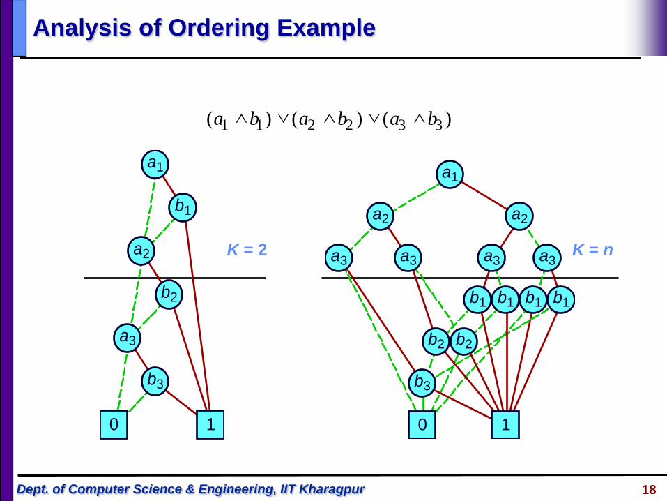
K = 2 K = n
0
b3
a3
b2
a2
1
b1
a1
a3 a3
a2
b1 b1
a3
b2
b1
0
b3
b2
1
b1
a3
a2
a1
Analysis of Ordering Example
)()()( 332211 bababa ∧∨∧∨∧

Dept. of Computer Science & Engineering, IIT Kharagpur 19
Selecting a good Variable Ordering
Intractable Problem■ Even when problem represented as OBDD
A good variable ordering should use■ Local computability■ Ordering based on power to control output
Application-Based Heuristics■ Exploit characteristics of application
● Ordering for functions of combinational circuit● Traverse circuit graph depth-first from outputs to
inputs● Assign variables to primary inputs in order
encountered
Dept. of Computer Science & Engineering, IIT Kharagpur 20
Dynamic Variable Ordering
Rudell, ICCAD ‘93
Concept■ Variable ordering changes as computation progresses
● Typical application involves long series of BDD operations
■ Proceeds in background, invisible to user
Implementation■ When approach memory limit, attempt to reduce
● Garbage collect unneeded nodes● Attempt to find better order for variables
■ Simple, greedy reordering heuristics
Dept. of Computer Science & Engineering, IIT Kharagpur 21
a3
b2 b2
a3
a2
a3
b1
b2
0
b3
b1
1
b2
a3
a2
a1
a3
b2
b3
b2
a3
a2
a3
b2
0
b1
b3
1
b2
a3
a2
a1
a2
a3
b1
b2
0
b3
b2
a3
1
b1
a2
a1
a3
b2
0
b3
b2
a3
a2
1
b1
a1
• • • a3
b2
0
b3
b2
a3
a2
1
a1
b1
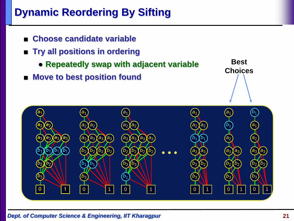
BestChoices
Dynamic Reordering By Sifting
■ Choose candidate variable■ Try all positions in ordering
● Repeatedly swap with adjacent variable■ Move to best position found

Dept. of Computer Science & Engineering, IIT Kharagpur 22
Function Class Best Worst Ordering SensitivityALU (Add/Sub) linear exponential HighSymmetric linear quadratic NoneMultiplication exponential exponential Low
General Experience■ Many tasks have reasonable OBDD representations■ Algorithms remain practical for up to 100,000 node OBDDs■ Heuristic ordering methods generally satisfactory
Sample Function Classes

Dept. of Computer Science & Engineering, IIT Kharagpur 23
BDD Operations
Strategy■ Represent data as set of OBDDs
● Identical variable orderings■ Express solution method as sequence of symbolic operations■ Implement each operation by OBDD manipulation
Algorithmic Properties■ Arguments are OBDDs with identical variable orderings.■ Result is OBDD with same ordering.■ “Closure Property”

Dept. of Computer Science & Engineering, IIT Kharagpur 24
The APPLY Operation
Given argument functions f and g, and a binary operator <op>, APPLY returns the function f <op> g
Works by traversing the argument graphs depth first
Algebraic operations “commute” with the Shannon expansion for any variable x■ f <op> g = x’ (f|x=0 <op> g|x=0 ) + x ((f|x=1 <op> g|x=1)

Dept. of Computer Science & Engineering, IIT Kharagpur 25
The Apply Algorithm
Consider a function f represented by a BDD with root vertex rf
The restriction of f with respect to a variable x such that x ≤ var(rf) can be computed as :
f | x = b = rf , x < var(rf )
= lo(rf), x = var (rf) and b = 0
= hi(rf), x = var (rf) and b = 1
The algorithm for APPLY utilizes the above restriction definition.

Dept. of Computer Science & Engineering, IIT Kharagpur 26
The Apply Algorithm
Each evaluation step is identified by a vertex from each of the argument graphs
Suppose functions f and g are represented by root vertices rf and rg
If rf and rg are both terminal vertices, terminate and return an appropriately labeled terminal vertex e.g. (A4, B3) and (A5, B4)

Dept. of Computer Science & Engineering, IIT Kharagpur 27
The Apply algorithm
Let x be the splitting variable
( x= min(var(rf) , var(rg))
BDDs for (f|x=0 <op> g|x=0 ) and (f|x=1 <op> g|x=1 ) are computed by recursively evaluating the restrictions of f and g for value 0 and for value 1

Dept. of Computer Science & Engineering, IIT Kharagpur 28
Recursive Calls
Example
Initial evaluation with vertices A1, B1 causes recursive evaluations with vertices A2, B2 and A6, B5
b
0
d
1
c
a
A4 A5
A3
A2
A6
A1
0 1
d
c
a
B3 B4
B2
B5
B1
A4,B3 A5,B4
A3,B2
A6,B2
A2,B2
A3,B4A5,B2
A6,B5
A1,B1

Dept. of Computer Science & Engineering, IIT Kharagpur 29
Apply operation
Reaching a terminal with a dominant value (e.g 1 for OR, 0 for AND) terminates recursion and returns an appropriately labeled terminal (A5, B2 and A3, B4)
Avoid multiple recursive calls on the same pair of arguments by a hash table (A3, B2 and A5, B2)

Dept. of Computer Science & Engineering, IIT Kharagpur 30
Apply operation
Each evaluation step returns a vertex in the generated graph
Apply reduction before merging the result
Complexity of operation : O(mf * mg) where mf and mg represent the number of vertices in the BDDs for f and g respectively

Dept. of Computer Science & Engineering, IIT Kharagpur 31
Recursive Calls Without Reduction With Reduction
Example
A4,B3 A5,B4
A3,B2
A6,B2
A2,B2
A3,B4A5,B2
A6,B5
A1,B1
0 1
d
c
b
11
c
a
C2
C4
C5
C3
C6
C1 0
d
c
b
1
a

Dept. of Computer Science & Engineering, IIT Kharagpur 32
Concept■ Effect of setting function argument xi to constant k (0 or 1).■ Also called Cofactor operation
k F xi –1
xi +1
xn
x1
F [xi =k]Fx equivalent to F [x = 1]Fx equivalent to F [x = 0]
Restrict Operation

Dept. of Computer Science & Engineering, IIT Kharagpur 33
Implementation
Depth-first traversal
Redirect any arc into vertex v having var(v) = x to point to hi(v) for x =1 and lo(v) for x = 0
Complexity linear in argument graph size
Restriction Algorithm

Dept. of Computer Science & Engineering, IIT Kharagpur 34
Argument F
Restriction Execution Example
0
a
b
c
d
1 0
a
c
d
1
Restriction F[b=1]
0
c
d
1
Reduced Result
Dept. of Computer Science & Engineering, IIT Kharagpur 35
■ Express as combination of Apply and Restrict
■ Preserve closure property●Result is an OBDD with the right variable
ordering
■ Polynomial complexity●Although can sometimes improve with special
implementations
Derived Operations

Dept. of Computer Science & Engineering, IIT Kharagpur 36
xi –1
xi +1
xn
x1
F ∃ ∃ xi F
1 F
0 F
xi –1
xi +1
xn
x1
xi –1
xi +1
xn
x1
Variable Quantification
■ Eliminate dependency on some argument through quantification
■ Combine with AND for universal quantification.

Dept. of Computer Science & Engineering, IIT Kharagpur 37
Digital Applications of BDDs
Verification■ Combinational equivalence (UCB, Fujitsu, Synopsys, …)
■ FSM equivalence (Bull, UCB, MCC,Colorado, Torino, …)
■ Symbolic Simulation (CMU, Utah)
■ Symbolic Model Checking (CMU, Bull, Motorola, …)
Synthesis■ Don’t care set representation (UCB, Fujitsu, …)
■ State minimization (UCB)
■ Sum-of-Products minimization (UCB, Synopsys, NTT)
Test
■ False path identification (TI)

Dept. of Computer Science & Engineering, IIT Kharagpur 38
Some Popular BDD packages
CUDD (Colorado University Decision Diagram)
TUD BDD package (TUDD)
BUDDY
CMU BDD
Informations about the above BDD packages and somemore details can be found at http://www.bdd-portal.org/

Dept. of Computer Science & Engineering, IIT Kharagpur 39
Finite State System Analysis
Systems Represented as Finite State Machines
■ Analysis Tasks■ State reachability■ State machine comparison■ Temporal logic model checking
Traditional Methods Impractical for Large Machines
■ Polynomial in number of states■ Number of states exponential in number of state variables.■ Example: single 32-bit register has 4,294,967,296 states!

Dept. of Computer Science & Engineering, IIT Kharagpur 40
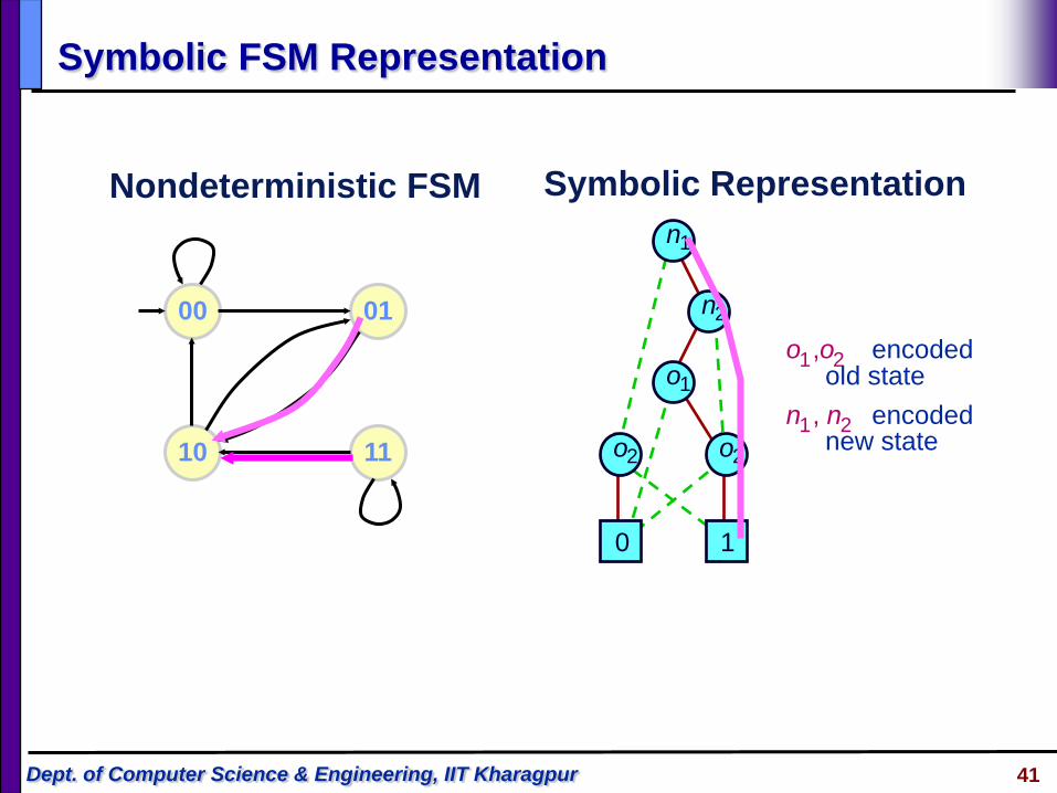
Symbolic FSM Representation
■ Represent set of transitions as function δ(Old, New)
● Yields 1 if can have transition from state Old to state New
■ Represent as Boolean function● Use variables for encoding states
Dept. of Computer Science & Engineering, IIT Kharagpur 41
Nondeterministic FSM Symbolic Representation
o1,o2 encodedold state
n1, n2 encodednew state
00
10
01
11 o2
o1
1
n2
0
n1
o2
Symbolic FSM Representation

Dept. of Computer Science & Engineering, IIT Kharagpur 42
Rstate 0/1δold state
new state0/1
Given Compute
InitialR0
=
Q0
Reachability Analysis
• Compute set of states reachable from initial state (Q0 = 00)
• Represent as Boolean function R(S)

Dept. of Computer Science & Engineering, IIT Kharagpur 43
R0
00
Breadth-First Reachability Analysis
■ Ri – set of states that can be reached in i transitions■ Reach fixed point when Rn = Rn+1
● Guaranteed since finite state
00
10
01
11
R1R0
00 01
R2R1R0
00 01 10
R3R2R1R0
00 01 10

Dept. of Computer Science & Engineering, IIT Kharagpur 44
■ Ri +1 – set of states that can be reached within i +1 transitions● Either in Ri
● or single transition away from some element of Ri
Ri
δ
Ri
∃
Ri +1
old
new
Iterative Computation

Dept. of Computer Science & Engineering, IIT Kharagpur 45
Example: Computing R1 from R0
o2
o1
1
n2
0
n1
o2
R0
00
R1
00 01
∃ Old [R0(Old) ∧ δ(Old, New)]
1
n2
0
n1
0
1
n2
0
n1
0 1 0
n1

Dept. of Computer Science & Engineering, IIT Kharagpur 46
Powerful Operations■ Creating, manipulating, testing■ Each step polynomial complexity
● Graceful degradation■ Maintain “closure” property
● Each operation produces form suitable for further operations
Generally Stay Small Enough■ Especially for digital circuit applications■ Given good choice of variable ordering
Weak Competition
What’s good about OBDDs ?

Dept. of Computer Science & Engineering, IIT Kharagpur 47
Doesn’t Solve All Problems■ Can’t do much with multipliers■ Some problems just too big■ Weak for search problems
Must be Careful■ Choose good variable ordering■ Some operations too hard
What’s not good about OBDDs?

Dept. of Computer Science & Engineering, IIT Kharagpur 48
Zero Suppressed BDD’s - ZBDD’s
ZBDD’s were invented by Minato to efficiently represent sparsesets. They have turned out to be extremely useful in implicit methods for representing primes (which usually are a sparse subset of all cubes).
Different reduction rules.

Dept. of Computer Science & Engineering, IIT Kharagpur 49
Zero Suppressed BDD’s - ZBDD’s
ZBDD Reduction Rule:: eliminate all nodes where the thennode points to 0. Connect incoming edges to else node
For ZBDD, equivalent nodes can be shared as in case of BDDs.
0 1
ZBDD:0
1
0 1
0

Dept. of Computer Science & Engineering, IIT Kharagpur 50
x0 + 2x1 + 4x2
Evaluating a MTBDD for a given variable assignment is similar to that in case of BDD
Very inefficient for representing functions yielding values over a large range
0 1
x0
2 3
x0
x1
4 5
x0
6 7
x0
x1
x2
MTBDD- Multiterminal BDD

Dept. of Computer Science & Engineering, IIT Kharagpur 51
EVBDD – Edge value BDD
EVBDDs can be used when the number of possible function values are too high for MTBDDs.
Evaluating a EVBDD involves tracing a path determined by the variable assignment, summing the weights and the terminal node value
g
x2
4
2
x1
x0
0 1

Dept. of Computer Science & Engineering, IIT Kharagpur 52
*BMD( Binary Moment Diagrams )
Features ■ Used for Word level simulation/verification■ Canonical■ Based on linear decomposition of a function
Functional Decomposition :f = (1-x) f~x + (x) fx
= f~x + x ( fx - f~x) = f~x + x ( f.x )
where f.x is the linear moment w.r.t. x
Dept. of Computer Science & Engineering, IIT Kharagpur 53
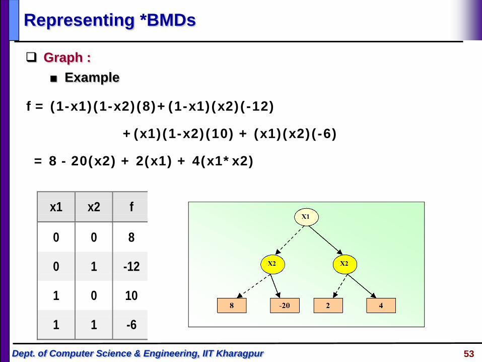
Representing *BMDs
Graph :■ Example
x1 x2 f
0 0 8
0 1 -12
1 0 10
1 1 -6
f = (1-x1)(1-x2)(8)+(1-x1)(x2)(-12)
+(x1)(1-x2)(10) + (x1)(x2)(-6)
= 8 - 20(x2) + 2(x1) + 4(x1*x2)

Dept. of Computer Science & Engineering, IIT Kharagpur 54
Weights combine multiplicatively along path from root to leaf Rules : weights of 2 branches relatively prime weight 0 allowed only for terminal vertices if one edge has weight 0, the other has weight 1
x
y y
8 -202 4
x
yy
1-5 2
2
2
BMD
* BMD
Edge Weights ( *BMDs )

Dept. of Computer Science & Engineering, IIT Kharagpur 55
References
Graph Based Algorithms for Boolean Function Manipulation,
Randal E. Bryant, IEEE Transactions on Computers, Volume: C-35, Issue: 8, pp. 677-
691, August 1986.
Symbolic Boolean Manipulation with Ordered Binary Decision
Diagrams,
Randal E. Bryant, ACM Computing Surveys, Volume: 24 Issue: 3, pp. 293-318,
September 1992.
An Introduction to Binary Decision Diagrams,
Henrik Reif Andersen, Technical Report, Course Notes on the WWW, October 1997.


![GaAs and InGaAs Single Electron Hexagonal Nanowire ...€¦ · Q-LSIs based on the binary-decision-diagram (BDD) logic architecture[3], using arrays of GaAs and InGaAs SE BDD node](https://static.fdocuments.net/doc/165x107/5f8f1c35fcaa4a5a3265bd37/gaas-and-ingaas-single-electron-hexagonal-nanowire-q-lsis-based-on-the-binary-decision-diagram.jpg)


