Bilinear Dynamical Systems

W. Penny1, Z. Ghahramani2 and K. Friston1

Wellcome Department of Imaging Neuroscience1,Gatsby Computational Neuroscience Unit2,University College, London WC1N 3BG.

February 11, 2005

AbstractIn this paper we propose the use of Bilinear Dynamical Systems

(BDS) for model-based deconvolution of fMRI time series. The impor-tance of this work lies in being able to deconvolve hemodynamic time-series, in an informed way, to disclose the underlying neuronal activity.Being able to estimate neuronal responses in a particular brain regionis fundamental for many models of functional integration and connec-tivity in the brain. BDSs comprise a stochastic bilinear neurodynami-cal model specified in discrete-time and a set of linear convolution ker-nels for the hemodynamics. We derive an Expectation-Maximisation(EM) algorithm for parameter estimation, in which fMRI time seriesare deconvolved in an E-step and model parameters are updated inan M-Step. We report preliminary results that focus on the assumedstochastic nature of the neurodynamic model and compare the methodto Wiener deconvolution.

Keywords: fMRI, Deconvolution, Connectivity, EM, Dynamical, Em-bedding

1 Introduction

Imaging neuroscientists have at their disposal a variety of imaging techniquesfor investigating human brain function [8]. The Electroencephalogram (EEG)

100

records electrical activity from electrodes placed on the scalp, the Magne-toencephalogram (MEG) records the magnetic field from sensors placed justabove the head and functional Magnetic Resonance Imaging (fMRI) recordschanges in magnetic resonances due to variations in blood oxygenation. How-ever, as the goal of brain imaging is to obtain information about the neu-ronal networks that support perceptual inference and cognition, one mustfirst transform measurements from imaging devices into estimates of intrac-erebral electrical activity. Brain imaging methodologists are therefore facedwith an inverse problem, ‘How can one make inferences about intracerebralneuronal processes given extracerebral/vascular measurements ?’

Though not often expressed in this terminology, we argue that this prob-lem is best formulated as a model-based spatio-temporal deconvolution prob-lem. For EEG and MEG the required deconvolution is primarily spatial, andfor fMRI it is primarily temporal. Although one can make minimal assump-tions about the source signals by applying ‘blind’ deconvolution methods[23, 24], knowledge of the underlying physical processes can be used to greateffect. This information can be implemented in a forward model that is in-verted during deconvolution. In EEG/MEG, forward models make use ofMaxwell’s equations governing propagation of electromagnetic fields [1], andin fMRI, forward models comprise hemodynamic processes as described by‘Balloon’ models [4, 9, 28, 30].

In this paper, we propose a new state-space method [18] for model-baseddeconvolution of fMRI. The importance of this work lies in being able todeconvolve hemodynamic time-series, in an informed way, to disclose the un-derlying neuronal activity. Such estimates are required by many models offunctional integration and connectivity in the brain. Typically, the influenceof an experimental manipulation, on the coupling between two regions, istested using a statistical model of the interaction between the experimentalfactor and neuronal activity in the source region. These interaction termsrest on being able to deconvolve the fMRI time-series. The procedures de-scribed below enable the construction of precise and informed interactionterms that can then be used to detect context sensitive coupling among brainregions. The interaction terms are variously known as PsychophysiologicalInteractions [10], moderator variables in Structural Equation Models [3], andbilinear inputs in Dynamic Causal Models [11].

The model we propose is called a Bilinear Dynamical System (BDS) andcomprises the following elements. Experimental manipulation (input) causeschanges in neuronal activation (state) which in turn cause changes in fMRI

101

signal (output). Experimental inputs fall into two classes (i) driving in-puts which directly excite neurodynamics and (ii) modulatory inputs whichchange the neurodynamics. These modulatory inputs typically correspondto instructional or attention set, and therefore allow neurodynamic changesto be directly attributed to changes in experimental context. Readers of ourearlier papers on Dynamic Causal Modelling (DCM) [11, 25] may well beexperiencing a sense of ‘deja-vu’. This is no accident because BDS employsthe same concepts of driving and modulatory inputs, neuronal states andoutputs.

A key difference to DCM, however, is that BDS uses a stochastic neu-rodynamic model. This is biologically more realistic as regional dynamicsare unlikely to be under full experimental control. Moreover, it has beenestablished, across a variety of spatial scales, that neurodynamics can bemeaningfully treated as stochastic processes, from Poisson processes describ-ing spike generation [6] to statistical mechanical treatments of activity incortical macrocolumns [21]. Stochastic components could also be consideredas the consequence of local or global deterministic nonlinear dynamics of apossibly chaotic nature (see eg. [2]). From another perspective, stochasticcomponents could be considered as reflecting input from remote regions [5].

In BDS, neurodynamics cause changes in fMRI signals via hemodynamicmodels specified in terms of a set of basis functions. Although more detaileddifferential equation models exist [4, 9, 28], the relationship between neuronalactivation and fMRI signals can be formulated as a first-order convolutionwith a kernel expansion using basis functions (typically two or three). Thiskernel is the hemodynamic response function. This approach has enjoyed adecade of empirical success in the guise of the General Linear Model (GLM)[12, 19]. Moreover, this means that the state-output relation can be describedby a linear convolution.

The BDS model may be viewed as a marriage of two formulations, theinput-state relation being a stochastic DCM and the state-output relationbeing a GLM.

BDS has a similar form to models used in signal processing and ma-chine learning. In particular, BDS is almost identical to a Linear DynamicalSystem (LDS) [29] with inputs. The only difference is that the inputs canchange the linear dynamics in a bilinear fashion - hence the name ‘Bilin-ear’ Dynamical Systems. In such models, the hidden variable, which in ourcase corresponds to the neuronal time series, can be estimated using Kalmansmoothing. Further, the parameters of the model can be estimated using

102

an Expectation-Maximisation (EM) algorithm described in [15] which needsonly minor modification to accomodate the bilinear term.

The structure of the paper is as follows. In section 2 we define BDS anddescribe how it can be applied to deconvolve fMRI time series. We describea novel EM algorithm for estimation of model parameters. In section 3 wepresent preliminary results on applying the models to synthetic data anddata from an fMRI experiment.

1.1 Notation

We denote matrices and vectors with bold upper case and bold lower caseletters respectively. All vectors are column vectors. XT denotes the trans-pose of X and Ik is the k-dimensional identity matrix. Brackets are used todenote entries in matrices/vectors. For example, A(i) denotes the ith row ofA, A(i, j) denotes the scalar entry in the ith row and jth column, and a(i)denotes the ith entry in a. We define zN as a vector with a 1 as the firstentry followed by N −1 zeros and 0I,J as the zero matrix of dimension I×J .

2 Bilinear Dynamical Systems

Although, in principle, we could define models for activity in a network ofregions, in this paper we define a BDS model for activity in only a singleregion. BDS is an input-state-output model where the states correspond to‘neuronal’ activations. Neuronal activity is defined mathematically belowand can be thought of as that component of the Local Field Potential (LFP)to which fMRI is most sensitive [22]. BDS is defined, for a single region, withthe following state-space equations where n indexes time

sn =(a + bT un

)sn−1 + dT vn + wn (1)

xn = [sn, sn−1, sn−2, .., sn−L+1]T (2)

yn = βTΦxn + en (3)

The first equation describes the stochastic neurodynamic model. Driving in-puts vn cause an increase in neuronal activity sn (a scalar) that decays with atime constant determined by (a+bT un). This time constant is determined bythe value of the ‘intrinsic connection’, a, and ‘modulatory inputs’, un. Driv-ing inputs typically correspond to the presentation of experimental stimuli

103

and modulatory inputs typically correspond to instructional or attentionalset. The strengths of the driving and modulatory effects are determined bythe vectors of driving connections, d, and modulatory connections, b. Thedriving connections are also known as ‘input efficacies’. Neuronal activity isalso governed by zero-mean additive Gaussian noise, wn, having variance σ2

w.Neuronal activation then gives rise to fMRI time series according to the

second and third equations. The second equation defines an embedding pro-cess [32] in which neuronal activity over the last L time steps is placed inthe ‘buffer’, xn. The vector xn is referred to as an ‘embedded’ time serieswhere L is the embedding dimension. Neuronal activation, now described byxn, then gives rise to fMRI time series, yn, via a linear convolution processdescribed in the third equation. Equation 3 comprises a signal term βTΦxn

and a zero-mean Gaussian error term en with variance σ2e . The hth row of

matrix Φ defines the hth convolution kernel (ie. basis of the hemodynam-ics response function) and β(h) is the corresponding regression coefficient.Figure 1 shows a set of convolution kernels that have been used widely forthe analysis of fMRI data in the context of the GLM. Linear combinationsof these functions have been found empirically to account for most subject-to-subject and voxel-to-voxel variations in hemodynamic response [19, 20].

The model can perhaps be better understood by looking at the neuronaland hemodynamic time series that it generates. An example is shown inFigure 2. The model we have proposed, BDS, can be viewed as a combina-tion of two models (i) a stochastic, discrete-time version of DCM to describeneurodynamics and (ii) the GLM to describe hemodynamics. GLMs are wellestablished in the neuroimaging literature [8] and DCMs are becoming so.Consequently, the model choices we have made are informed by precedentsestablished for GLMs and DCMs. For example, from previous work usingGLMs [20], we know that the embedding dimension should be chosen to spana 20-30s period. With regard to neurodynamics, the discrete bilinear formaffords analytic tractability while allowing nonlinear interactions between ex-ogenous input and states. The splitting of exogenous inputs into driving andmodulatory terms is also prompted by DCM. The motivation for this is that,for data collected from controlled experiments, one wishes to relate changes inconnectivity to experimental manipulation. This distinction is echoed by theseparate neurobiological mechansisms underlying driving versus modulatoryactivity [25].

The modulatory coefficients in equation 1, b, are also known as ‘bilinear’terms. This is because the dependent variable, sn, is linearly dependent on

104

the product of sn−1 and un. That un and sn−1 combine in multiplicativefashion endows the model with ‘nonlinear’ dynamics that can be understoodas a nonstationary linear system that changes according to experimentalcontext. Importantly, because un is known, it is straightforward to estimatehow the dynamics are changing. We emphasise that the term ’bilinear’ relatesto interactions between a state and an input rather than among the statesthemselves.

2.1 Relation to biophysical models

In the previous section, we interpreted (a + bT un) as the time constant ofdecaying neuronal activity. However, our BDS model has a much moregeneral relationship to underlying biophysical models of neuronal dynam-ics. Consider some biologically plausible model of neuronal activity thatis formulated in continuous time x = f(x, u, θ) and allows for arbitrarilycomplicated and nonlinear effects of the state and exogenous inputs. Theparameters of this biophysical model θ (c.f. neural mass models [31]) can berelated directly to biophysical processes. In our discrete-time formulation,under local linearity assumptions, a = exp(∆t∂f/∂x) and b(i) = ∂a/∂u(i) =∆ta∂2f/∂x∂u(i) where ∆t is the sampling interval and i indexes the input.This means that our input-dependent autoregression coefficients can be re-garded as a lumped representation of the underlying model parameters. Thisre-parameterization, in terms of a state-space model, precludes an explicitestimation of the original parameters. However, this does not matter becausewe are not interested in the parameters per se; we only require the condi-tional estimates of the states. The transformation of a dynamic formulationinto a discrete BDS is a useful perspective because priors on the biophysicalparameters can be used to specify priors on the autoregression coefficients,should they be needed.

2.2 Relation to GLMs

For models with a single input BDS reduces to a GLM if sn = vn, that is, if theneuronal activity is synonymous with the experimental manipulation (drivinginputs). This highlights a key assumption of GLMs, that the dynamics ofneuronal transients can be ignored.

For models with multiple inputs the relation between BDS and GLMs ismore complex. Ignoring bilinear and noise terms, BDS can be more parsi-

105

monious than the GLM in the sense of having fewer parameters. Say, forexample, we are modelling hemodynamics with H basis functions. Then forM (driving) input variables, the GLM has HM parameters, whereas in BDS,there are M + H + 1 parameters. For H = 3, for example, BDS has fewercoefficients if M ≥ 3.

The reason for this reduction is that, in BDS, the inputs affect onlyneurodynamics. And the strength of this effect, ignoring modulatory terms,is captured in a single parameter, the input efficacy. The relation betweenneurodynamics and hemodynamics is independent of which input excitedneuronal activity. This is obviously more consistent with physiology whereexperimental manipulation only affects fMRI by changing neuronal activity.

2.3 Deconvolution

Deconvolution consists of estimating a neuronal time series, sn, given anfMRI time series, yn. It is possible to perform model-based deconvolutionusing BDS and a modified Kalman-filtering algorithm. The modification isnecessary because, due to the modulatory terms, the state transition ma-trix is time-dependent. Also, the BDS model must be reformulated so thatthe output is an instantaneous function of the state. This section describesstandard Kalman filtering and the modifications required for BDS.

In the Kalman-filtering approach, deconvolution progresses via iterativecomputation of the probability density p(sn|yn

1 ) where yn1 = {y1, y2, ...yn}.

That is, our estimate of neuronal activity at time step n is based on all thefMRI data up to time n (but not on future values).

The Kalman-filtering algorithm can be split into two steps that are ap-plied recursively. The first step is a time update where the density p(sn−1|yn−1

1 )is updated to p(sn|yn−1

1 ). In our model this will take into account the effectsof inputs un and vn and the natural decay of neuronal activity. The secondstep is a measurement update where the density p(sn|yn−1

1 ) is updated top(sn|yn

1 ) thereby taking into account the ‘new’ fMRI measurement yn. Thetwo steps together take us from time point n − 1 to time point n and areapplied recursively to deconvolve the entire time-series.

A complication arises, however, because the Kalman filtering updates re-quire that the output be an instantaneous function of the hidden state. Thatis, that yn depend only on sn and not on sn−1, sn−2 etc, which is clearlynot the case. But Kalman filtering can proceed if we use the embeddedstate variables xn. This will lead to an estimate of the multivariate den-

106

sity p(xn|yn1 ). Our desired density, p(sn|yn

1 ), is then just the first entry inp(xn|yn

1 ). Whilst this is conceptually simple, a good deal of book-keepingis required to translate the BDS neurodynamical model into an ‘embeddedspace’. This is described in detail in Appendices A and B.

A second complication arises in that, in the standard Kalman updateformulae [15], the inputs do not change the intrinsic dynamics. To accountfor this we introduce a time-dependent state-transition matrix that embodieschanges in intrinsic dynamics due to modulatory inputs. This is also detailedin Appendices A and B.

It is also possible to perform deconvolution based on Kalman-smoothingrather than Kalman-filtering. Kalman-smoothing estimates neuronal activityby computing the density p(sn|yN

1 ). It is therefore based on the whole fMRIrecord, ie. past and future values and, as we shall see, provides more accuratedeconvolutions in high noise environments.

2.4 Estimation

To run the deconvolution algorithms described in the previous section wemust know the parameters of the model eg. β, a, b and d. If these parametersare unknown, as will nearly always be the case, they can be estimated usingMaximum-Likelihood (ML) methods.

For BDS this can be implemented using an Expectation-Maximisation(EM) algorithm which we derive in Appendices A and B. The E-step uses aKalman smoothing algorithm which contains only minor modifications to thealgorithm presented in [15]. The M-step contains updates derived by consid-ering estimation of the neurodynamic parameters (a, b, d) as a constrainedlinear regression problem [27]. The neurodynamic parameters are updatedas shown in equation 25 and the hemodynamic parameters, β, are updatedusing equation 28. It is also possible to update the initial state estimatesas described in [15], but this was not implemented for the empirical work inthis paper.

It is also possible to implement ML parameter estimation by comput-ing the likelihood using Kalman filtering (as shown in Appendix C), andthen maximising this using standard Matlab optimisation algorithms such asPseudo-Newton or Simplex methods [26]. However, preliminary simulationsshowed EM to be faster than these other ML methods.

107

2.5 Initialisation

The EM estimation algorithm is initialised as follows. In the limit of ZeroNeuronal Noise (ZNN) the neuronal activity is given by

sn = (a + bT un)sn−1 + dT vn (4)

and the predicted hemodynamic activity is

yn = βTΦxn (5)

We intially set a to a random number between 0 and 1, and b such thatbT un is between 0 and 1−a for all n. The values of d are also set to randomnumbers between 0 and 1. The first β coefficient is fixed at unity, and others,if there are any, are initialised to random numbers between 0 and 1. We thenrun a pseudo-Newton gradient descent optimisation (the function fminunc inMatlab) to minimise the discrepancy between the observed fMRI time seriesyn and the estimated values yn under the ZNN assumption. Occasionally,parameter estimates result in an unstable model. We therefore repeat theseinitialisation steps until a stable model is returned. These parameters arethen used as a starting point for EM.

3 Results

3.1 Simulations

We generate simulated data to demonstrate various properties of the deconvo-lution algorithm. These simulations are similar to the first set of simulationsin [16]. We also compare our results to those obtained with Wiener deconvo-lution [17], which makes minimal assumptions about the source (that it hasa flat spectral density [26, 16]).

A 250s time series of input events with sampling period ∆t = 0.5s wasgenerated from a Poisson distribution with a mean interval between events of12s. Events less than 2s apart were then removed. The half-life of neuronaltransients was fixed to 1s by setting a = 0.71, the input efficacy was setto d = 0.9 and the neuronal noise variance was set to σ2

w = 0.0001. Therewere no modulatory coefficients and a single hemodynamic basis function(the ‘canonical’, shown in Figure 1) was used.

108

We then added observation noise to achieve a Signal to Noise Ratio (SNR)of unity (this is equivalent to the 100% noise case in [16]). This was achievedusing σ2

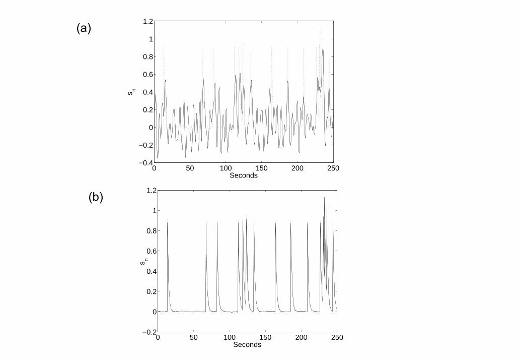
e = 0.015. The generated time series is shown in Figure 3.The parameters were estimated using EM to be a = 0.72 and d = 0.88.

Wiener and BDS Kalman smoothing deconvolutions (the latter obtained us-ing estimated parameters) are shown in Figure 4. Wiener deconvolution usedthe known value of σ2

e and BDS Kalman smoothing used the known values ofσ2

e and σ2w. The quality of the BDS deconvolution is considerably better than

that using the method described in [16] (see eg. Figure 3D in [16]). This isbecause information about the paradigm (eg. experimental inputs) has beenused. For Wiener deconvolution the correlation with the generated neuronaltime series is r = 0.520 and for BDS Kalman smoothing it is r = 0.998.

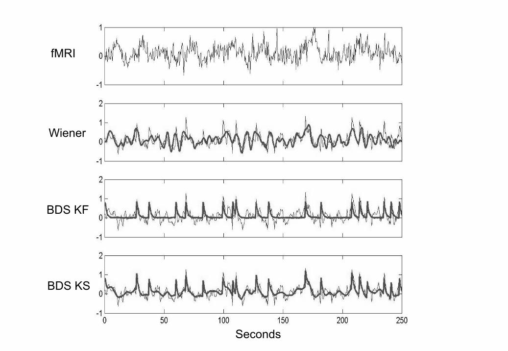
We then ran a second simulation with the neuronal noise variance set toa high value, σ2

w = 0.03. This data is shown in the top panel of Figure 5.Neurodynamic parameters were estimated, using EM, to be a = 0.68 andd = 0.83. For comparison, ZNN initialisation (see section 2.5) producedparameter estimates a = 0.45 and d = 1.13. That is, the assumption of zeroneuronal noise leads to an underestimate of the neuronal time constant andan overestimate of the input efficacy.

The neuronal time series, as estimated using BDS Kalman smoothing(bottom panel of Figure 5) had a correlation with the generated time seriesof r = 0.775. The ZNN estimate neuronal time series had a correlation of r =0.724. The Wiener deconvolved time series (second panel in Figure 5) gaver = 0.52 (again). We also show, in the third panel of Figure 5, deconvolutionsfrom BDS Kalman filtering.

Figure 5 shows that Wiener estimation recovers the intrinsic dynamicsbut misses the evoked responses, whereas BDS Kalman filtering recovers theevoked responses but misses the intrinsic dynamics. Deconvolution usingBDS Kalman smoothing recovers both.

The smoother can capture the intrinsic dynamics because it uses moreinformation than the filter. It updates the filter estimates of neuronal activ-ity, at a given time point, using information in advance of that time point(ie. from the future). These updates are implemented using the ‘backwardrecursions’ described in Appendix B.1. Heuristically, the reason for the im-provement is that the best estimates of neuronal activity are obtained usingobserved fMRI activity about 5 seconds or so in the future ie. at the peak ofthe hemodynamic response.

109

3.2 Single word processing fMRI

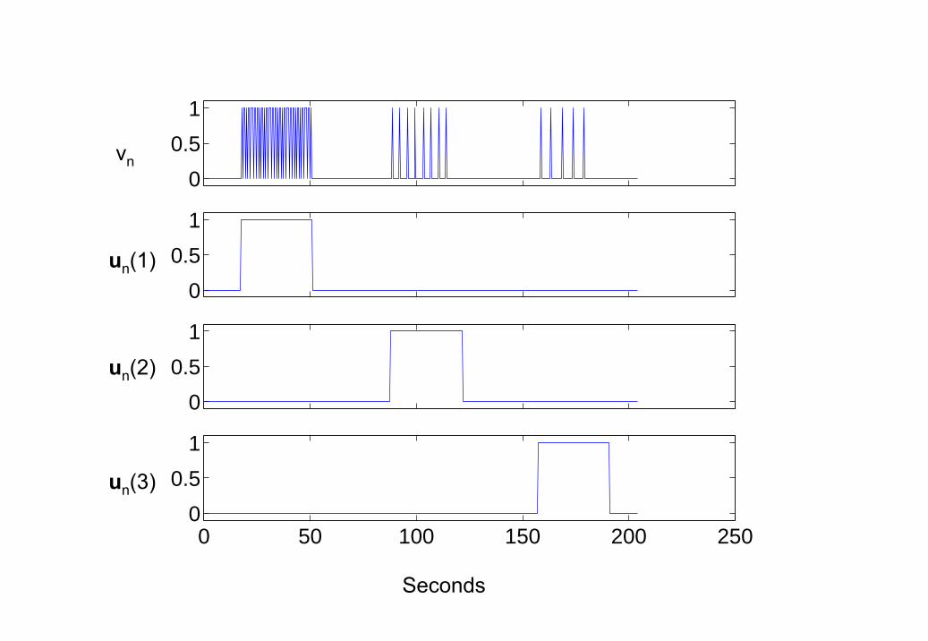
We now turn to the analysis of an fMRI data set recorded during a passivelistening task, using epochs of single words presented at different rates. Theexperimental inputs in Figure 6 describe the paradigm in more detail. Thedriving inputs in the top panel indicate presentation of words in the subject’sheadphones and modulatory inputs in the lower panels indicate epochs withdifferent presentation rates.

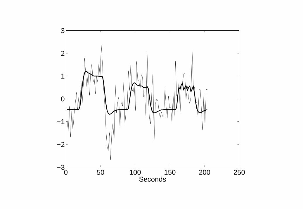
We focus on a single time series in primary auditory cortex shown inFigure 7. This comprises 120 time points with a sampling period ∆t = 1.7s.Further details of data collection are given in [11]. As the experimental inputsare specified at a higher temporal resolution than the fMRI acquisition, weupsampled the fMRI data by a factor of 4 prior to analysis. The inputvariables were convolved with a ‘canonical’ hemodynamic response function(see top panel of Figure 1) to form regressors in a GLM. Figure 7 shows theresulting GLM model fit.

The same input variables and hemodynamic basis function were then usedto define a BDS model. The observation and state noise variances were set toσ2

e = σ2w = 0.1, and the hemodynamic regression coefficient was set to β = 1.

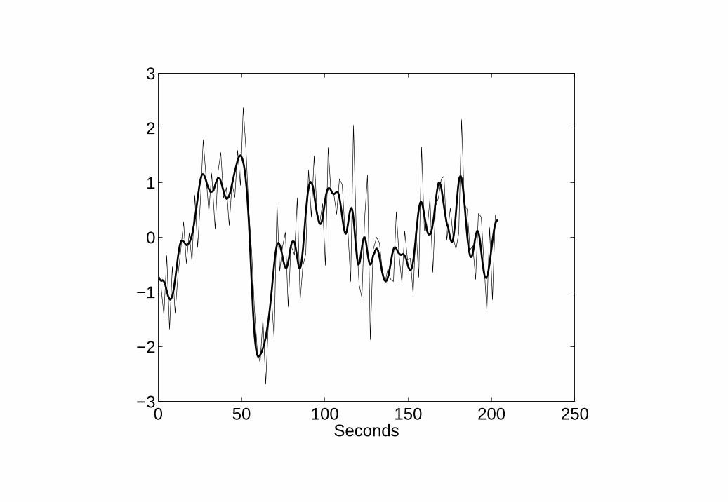
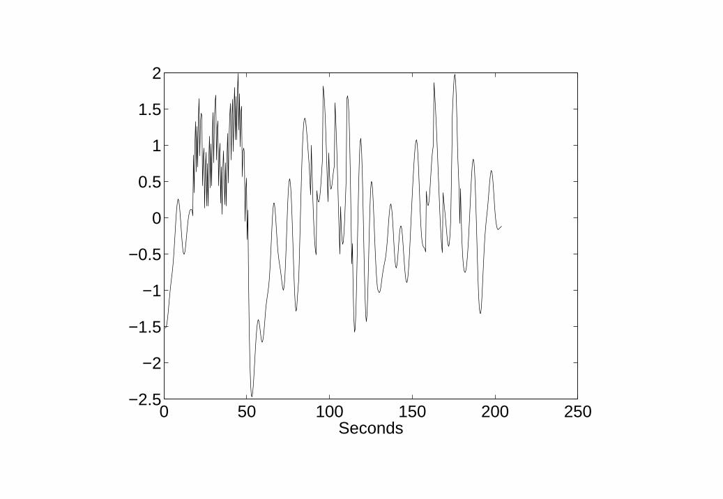
Figure 8 shows the resulting model fit which is clearly superior to the GLMmodel fit in Figure 7 (but see Discussion). Figure 9 shows neuronal activityas estimated using BDS Kalman smoothing. This includes both event-relatedresponses (the ’spikes’) and intrinsic activity (slow fluctuations).

Neurodynamic parameters were estimated, using EM, as d = 0.80, a =0.92, b(1) = −0.44, b(2) = −0.08 and b(3) = −0.02. Thus, epochs withfaster stimulus presentations were estimated to have an increasingly inhibitoryeffect on event-related neurodynamics. This pattern was robust across a widerange of settings of the noise variance parameters. This finding is consistentwith neuronal repetition suppression effects and is in agreement with Dy-namic Causal Modelling of this data [11].

4 Discussion

We have proposed a new algorithm, based on a Bilinear Dynamical Sys-tem (BDS), for model-based deconvolution of fMRI time series. The impor-tance of the work is that hemodynamic time-series can be deconvolved, inan informed way, to disclose the underlying neuronal activity. Being able

110

to estimate neuronal responses in a particular brain region is fundamentalfor many models of functional integration and connectivity in the brain. Ofcourse, these estimates can only describe those components of neuronal ac-tivity to which fMRI is sensitive. They should nevertheless be useful formaking fMRI-based assessments of connectivity [10, 16].

BDS is fitted to data using a novel Expectation-Maximisation (EM) algo-rithm where deconvolution is instantiated in an E-step and model parametersare updated in an M-step. Simulations showed EM to be faster than maxi-mum likelihood optimisation based on simplex or Pseudo-Newton methods.Deconvolution can be based either on a full E-step, using Kalman smoothing,or a partial E-step based on Kalman filtering. Kalman smoothing uses thefull data record wheras Kalman filtering only uses information from the past.

Simulations showed that our model-based deconvolution is more accuratethan blind deconvolution methods (Wiener filtering). This is because BDSuses information about the paradigm. We also observed the following trends.Wiener estimation recovers the intrinsic dynamics but misses the evokedresponses, whereas BDS Kalman filtering recovers the evoked responses butmisses the intrinsic dynamics. Deconvolution using BDS Kalman smoothingrecovers both.

Simulations also suggest that if dynamics are indeed of a stochastic na-ture, as is assumed in BDS, then if we mistakenly assume deterministicdynamics, estimation of neuronal efficicies and time constants will becomeinnaccurate. This has implications for models that assume deterministic dy-namics, such as DCM [11].

Our applications of BDS provide good examples of Kalman smoothingproviding better deconvolutions than Kalman filtering. The reason is thatsmoothing also uses future observations and the best estimates of neuronalactivity are obtained using observed fMRI activity about 5 seconds or so intothe future, that is, at the peak of the hemodynamic response. This propertyshould hold for any state-space model of fMRI (see eg. [28]).

A comparison of GLM and BDS model fits in figures 7 and 8 clearly showsthat BDS is superior. Whilst this is somewhat encouraging, this observationshould be tempered with a note of caution. This is because the BDS modelis more complex and no penalty was paid for this during model fitting. TheBDS model may therefore be overfitted. In particular, as fMRI time seriesare known to contain aliased cardiac and respiratory artifacts, the finer de-tails that BDS picks up may be of artifactual rather than neuronal origin.To eliminate this possibility one would need to estimate model parameters

111

(especially the state noise variance) using Bayesian or cross-validation [33]methods. Fortunately, Bayesian methods have already been developed forLinear Dynamical Systems [14] that should not require too many changes toaccomodate the bilinear term.

Recently, Riera et al. [28] have proposed a state-space model for fMRItime series which allows for nonlinear state-output relations. They showedhow model parameters could be estimated using a maximum likelihood pro-cedure based on Extended Kalman Filtering. Moreover, they showed howthe parameters could be related to a stochastic differential equation imple-mentation of the Balloon model. Thus, unlike BDS which assumes linearhemodynamics, their model can describe nonlinear properties such as hemo-dynamic refractoriness. This is important, as the neuronal refractorinessinferred using BDS in section 3.2, for example, may actually be of hemo-dynamic rather than neuronal origin. In fact, a Dynamic Causal Modellinganalysis of this data [11], which allows for both neuronal and hemodynamicrefractoriness, concluded that both effects were present.

The model proposed by Riera et al. [28] also differs from BDS in the input-state relations. In BDS, this is governed by driving inputs that excite linearneurodynamics which can be changed according to modulatory inputs. Thismeans that neurodynamics and changes in them can be directly attributedto changes in experimental context. This modelling approach is thereforeappropriate for designed experiments where the inputs are known. In theRiera model, the inputs are not assumed to be known. Instead, a moreflexible radial basis function approach is used to make inferences about theonsets of linear neurodynamical processes.

In previous work we have proposed an fMRI deconvolution model basedon the GLM [16]. This uses a forward model in which neuronal activity,represented using a temporal basis set and corresponding coefficients, is con-volved with a known hemodynamic kernel to produce an fMRI time series.Observation noise is then added. Deconvolution is achieved by estimatingthe coefficients of the temporal basis functions. In [16] we used full-rankFourier basis sets and overcomplete basis sets that used information aboutexperimental design. Coefficients were estimated using priors and Paramet-ric Empirical Bayes. A problem with the method, however, is that for Jcoefficients (where J is typically the length of the time series or longer) onemust store and invert J × J covariance matrices. A computational benefitof the BDS approach is that, by making use of factorisations that derivefrom Markov properties of the state-space model, one need only manipulate

112

L × L covariance matrices, where L is the temporal embedding dimension(L << J). We have also argued, in section 3.2, that BDS is more parsimo-nious and biologically informed than the GLM.

The method we have proposed has been applied to deconvolve data ata single voxel. This is useful in providing a ‘source’ neuronal time series,for example, for the analysis of PPIs [10, 16]. More generally, however, oneis interested in making inferences about changes in connectivity in neuralnetworks extended over multiple regions. This requires simultaneous decon-volution at multiple voxels and, ideally, a full model-based spatio-temporaldeconvolution. The application of state-space models to this more difficultproblem is an exciting area of current research (see eg. [13]).

Acknowledgements

Will Penny and Karl Friston are funded by the Wellcome Trust.

References

[1] S. Baillet, J.C. Mosher, and R.M. Leahy. Electromagnetic Brain Map-ping. IEEE Signal Processing Magazine, pages 14–30, November 2001.

[2] M. Breakspear and J.R. Terry. Nonlinear interdependence in neuralsystems: motivation, theory and relevance. International Journal ofNeuroscience, 112:1263–1284, 2002.

[3] C. Buchel and K.J. Friston. Modulation of connectivity in visual path-ways by attention: Cortical interactions evaluated with structural equa-tion modelling and fMRI. Cerebral Cortex, 7:768–778, 1997.

[4] R.B. Buxton, E.C. Wong, and L.R. Frank. Dynamics of blood flowand oxygenation changes during brain activation: The Balloon Model.Magnetic Resonance in Medicine, 39:855–864, 1998.

[5] O. David and K.J. Friston. A neural mass model for MEG/EEG: cou-pling and neuronal dynamics. NeuroImage, 20(3):1743–1755, 2003.

[6] P. Dayan and L.F. Abbott. Theoretical Neuroscience: Computationaland Mathematical Modeling of Neural Systems. MIT Press, 2001.

113

[7] A.P. Dempster, N.M. Laird, and D.B. Rubin. Maximum likelihood fromincomplete data via the EM algorithm. Journal of the Royal StatisticalSociety B, 39:1–38, 1977.

[8] R.S.J. Frackowiak, K.J. Friston, C. Frith, R. Dolan, C.J. Price, S. Zeki,J. Ashburner, and W.D. Penny, editors. Human Brain Function. Aca-demic Press, 2003. 2nd Edition.

[9] K.J. Friston. Bayesian estimation of dynamical systems: An applicationto fMRI. NeuroImage, 16:513–530, 2002.

[10] K.J. Friston, C. Buchel, G.R. Fink, J. Morris, E. Rolls, and R. Dolan.Psychophysiological and modulatory interactions in neuroimaging. Neu-roImage, 6:218–229, 1997.

[11] K.J. Friston, L. Harrison, and W.D. Penny. Dynamic Causal Modelling.NeuroImage, 19(4):1273–1302, 2003.

[12] K.J. Friston, A.P. Holmes, K.J. Worsley, J.B. Poline, C. Frith, andR.S.J. Frackowiak. Statistical parametric maps in functional imaging:A general linear approach. Human Brain Mapping, 2:189–210, 1995.

[13] A. Galka, O. Yamashita, T. Ozaki, R.Biscay, and P. Valdes-Sosa. Asolution to the dynamical inverse problem of EEG generation using spa-tiotemporal Kalman filtering. NeuroImage, 2004. In Press.

[14] Z. Ghahramani and M.J. Beal. Propagation algorithms for VariationalBayesian learning. In T. Leen et al, editor, NIPS 13, Cambridge, MA,2001. MIT Press.

[15] Z. Ghahramani and G.E. Hinton. Parameter Estimation for LinearDynamical Systems. Technical Report CRG-TR-96-2, Department ofComputer Science, University of Toronto, 1996. Also available fromhttp://www.gatsby.ucl.ac.uk/∼zoubin/papers.html.

[16] D.R. Gitelman, W.D. Penny, J. Ashburner, and K.J. Friston. Modelingregional and psychophsyiologic interactions in fMRI: the importance ofhemodynamic deconvolution. NeuroImage, 19:200–207, 2003.

[17] G.H. Glover. Deconvolution of impulse response in event-related BOLDfMRI. NeuroImage, 9:416–429, 1999.

114

[18] S. Haykin. Adaptive Filter Theory, 3rd Edition. Prentice-Hall, 1996.

[19] R.N.A. Henson. Human Brain Function, chapter 40. Academic Press,2003. 2nd Edition.

[20] R.N.A. Henson, M.D. Rugg, and K.J. Friston. The choice of basis func-tions in event-related fMRI. NeuroImage, 13(6):127, June 2001. Sup-plement 1.

[21] L. Ingber. Statistical mechanics of multiple scales of neocortical inter-actions. In P. Nunez, editor, Neocortical dynamics and human EEGrhythms. Oxford University Press, 1995.

[22] N.K. Logothetis, J. Pauls, M. Augath, T. Trinath, and A. Oeltermann.Neurophysiological investigation of the basis of the fMRI signal. Nature,412:150–157, 2001.

[23] S. Makeig, M. Westerfield, T.-P. Jung, S. Enghoff, J. Townsend,E. Courchesne, and T.J. Sejnowski. Dynamic brain sources of visualevoked responses. Science, 295:690–694, 2002.

[24] M.J. McKeown, S. Makeig, G.G. Brown, T.P. Jung, S.S. Kindermann,A.J. Bell, and T.J. Sejnowski. Analysis of fMRI data by blind separationinto independent spatial components. Human Brain Mapping, 6:160–188, 1998.

[25] W.D. Penny, K.E. Stephan, A. Mechelli, and K.J. Friston. ComparingDynamic Causal Models. NeuroImage, 22(3):1157–1172, 2004.

[26] W. H. Press, S.A. Teukolsky, W.T. Vetterling, and B.V.P. Flannery.Numerical Recipes in C. Cambridge, 1992.

[27] C.R Rao and H. Toutenberg. Linear Models: Least squares and alter-natives. Springer, 1995.

[28] J. Riera, J. Watanabe, K. Iwata, N. Miura, E. Aubert, T. Ozaki, andR. Kawashima. A state-space model of the hemodynamic approach:nonlinear filtering of BOLD signals. NeuroImage, 21:547–567, 2004.

[29] S. Roweis and Z. Ghahramani. A unifying review of linear gaussianmodels. Neural Computation, 11(2):305–346, 1999.

115

[30] K.E. Stephan, L. Harrison, W.D. Penny, and K.J. Friston. Biophysicalmodels of fMRI responses. Current Opinion in Neurobiology, 14(5):629–635, 2004.

[31] P.A. Valdes, J.C. Jimenez, J. Riera, R. Biscay, and T. Ozaki. NonlinearEEG analysis based on a neural mass model. Biological Cybernetics,81:415–424, 1999.

[32] A.S. Weigend and N.A. Gershenfeld. Time series prediction: forecastingthe future and understanding the past. Addison-Wesley, 1994.

[33] O. Yamashita, A. Galka, T. Ozaki, R. Biscay, and P. Valdes-Sosa. Re-cursive penalised least squares solution for dynamical inverse problemsof EEG generation. Human Brain Mapping, 21:221–235, 2004.

116

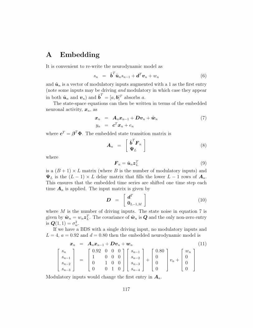
A Embedding

It is convenient to re-write the neurodynamic model as

sn = bTunsn−1 + dT vn + wn (6)

and un is a vector of modulatory inputs augmented with a 1 as the first entry(note some inputs may be driving and modulatory in which case they appear

in both un and vn) and bT

= [a, b]T absorbs a.The state-space equations can then be written in terms of the embedded

neuronal activity, xn, as

xn = Anxn−1 + Dvn + wn (7)

yn = cT xn + en

where cT = βTΦ. The embedded state transition matrix is

An =

[b

TF n

ΨL

](8)

whereF n = unz

TL (9)

is a (B + 1)× L matrix (where B is the number of modulatory inputs) andΨL is the (L − 1) × L delay matrix that fills the lower L − 1 rows of An.This ensures that the embedded time series are shifted one time step eachtime An is applied. The input matrix is given by

D =

[dT

0L−1,M

](10)

where M is the number of driving inputs. The state noise in equation 7 isgiven by wn = wnz

TL. The covariance of wn is Q and the only non-zero entry

is Q(1, 1) = σ2w.

If we have a BDS with a single driving input, no modulatory inputs andL = 4, a = 0.92 and d = 0.80 then the embedded neurodynamic model is

xn = Anxn−1 + Dvn + wn (11)sn

sn−1

sn−2

sn−3

=

0.92 0 0 01 0 0 00 1 0 00 0 1 0

sn−1

sn−2

sn−3

sn−4

+

0.80000

vn +

wn

000

Modulatory inputs would change the first entry in An.

117

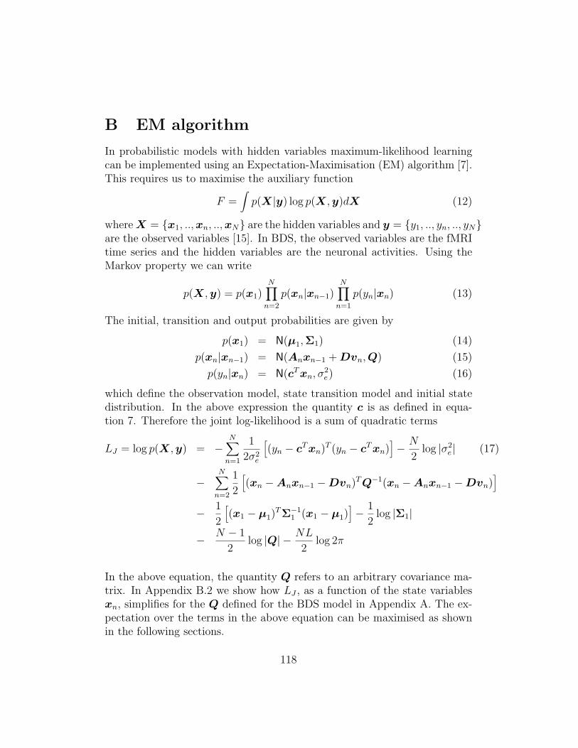
B EM algorithm

In probabilistic models with hidden variables maximum-likelihood learningcan be implemented using an Expectation-Maximisation (EM) algorithm [7].This requires us to maximise the auxiliary function

F =∫

p(X|y) log p(X, y)dX (12)

where X = {x1, ..,xn, ..,xN} are the hidden variables and y = {y1, .., yn, .., yN}are the observed variables [15]. In BDS, the observed variables are the fMRItime series and the hidden variables are the neuronal activities. Using theMarkov property we can write

p(X, y) = p(x1)N∏

n=2

p(xn|xn−1)N∏

n=1

p(yn|xn) (13)

The initial, transition and output probabilities are given by

p(x1) = N(µ1,Σ1) (14)

p(xn|xn−1) = N(Anxn−1 + Dvn, Q) (15)

p(yn|xn) = N(cT xn, σ2e) (16)

which define the observation model, state transition model and initial statedistribution. In the above expression the quantity c is as defined in equa-tion 7. Therefore the joint log-likelihood is a sum of quadratic terms

LJ = log p(X, y) = −N∑

n=1

1

2σ2e

[(yn − cT xn)T (yn − cT xn)

]− N

2log |σ2

e | (17)

−N∑

n=2

1

2

[(xn −Anxn−1 −Dvn)T Q−1(xn −Anxn−1 −Dvn)

]− 1

2

[(x1 − µ1)

TΣ−11 (x1 − µ1)

]− 1

2log |Σ1|

− N − 1

2log |Q| − NL

2log 2π

In the above equation, the quantity Q refers to an arbitrary covariance ma-trix. In Appendix B.2 we show how LJ , as a function of the state variablesxn, simplifies for the Q defined for the BDS model in Appendix A. The ex-pectation over the terms in the above equation can be maximised as shownin the following sections.

118

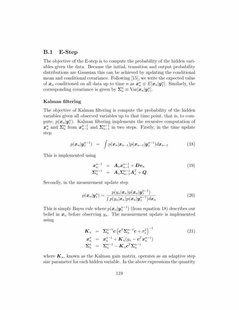
B.1 E-Step

The objective of the E-step is to compute the probability of the hidden vari-ables given the data. Because the initial, transition and output probabilitydistributions are Gaussian this can be achieved by updating the conditionalmean and conditional covariance. Following [15], we write the expected valueof xn conditioned on all data up to time n as xn

n ≡ E[xn|yn1 ]. Similarly, the

corresponding covariance is given by Σnn ≡ Var[xn|yn

1 ].

Kalman filtering

The objective of Kalman filtering is compute the probability of the hiddenvariables given all observed variables up to that time point, that is, to com-pute, p(xn|yn

1 ). Kalman filtering implements the recursive computation ofxn

n and Σnn from xn−1

n−1 and Σn−1n−1 in two steps. Firstly, in the time update

step

p(xn|yn−11 ) =

∫p(xn|xn−1)p(xn−1|yn−1

1 )dxn−1 (18)

This is implemented using

xn−1n = Anx

n−1n−1 + Dvn (19)

Σn−1n = AnΣ

n−1n−1A

Tn + Q

Secondly, in the measurement update step

p(xn|yn1 ) =

p(yn|xn)p(xn|yn−11 )∫

p(yn|xn)p(xn|yn−11 )dxn

(20)

This is simply Bayes rule where p(xn|yn−11 ) (from equation 18) describes our

belief in xn before observing yn. The measurement update is implementedusing

Kn = Σn−1n c

(cTΣn−1

n c + σ2e

)−1(21)

xnn = xn−1

n + Kn(yn − cT xn−1n )

Σnn = Σn−1

n −KncTΣn−1

n

where Kn, known as the Kalman gain matrix, operates as an adaptive stepsize parameter for each hidden variable. In the above expressions the quantity

119

c is as defined in equation 7. The procedure is initialised using x01 = µ1 and

Σ01 = Σ1. These updates are exactly as described in [15] except that (i) An

is used instead of A because our dynamics are input-dependent, and (ii) weuse c instead of C because our observations are univariate.

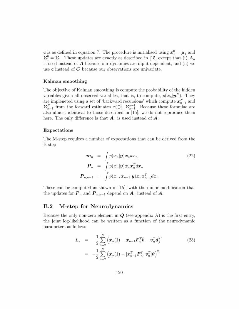
Kalman smoothing

The objective of Kalman smoothing is compute the probability of the hiddenvariables given all observed variables, that is, to compute, p(xn|yN

1 ). Theyare impleneted using a set of ‘backward recursions’ which compute xN

n−1 andΣN

n−1 from the forward estimates xn−1n−1, Σn−1

n−1. Because these formulae arealso almost identical to those described in [15], we do not reproduce themhere. The only difference is that An is used instead of A.

Expectations

The M-step requires a number of expectations that can be derived from theE-step

mn =∫

p(xn|y)xndxn (22)

P n =∫

p(xn|y)xnxTndxn

P n,n−1 =∫

p(xn, xn−1|y)xnxTn−1dxn

These can be computed as shown in [15], with the minor modification thatthe updates for P n and P n,n−1 depend on An instead of A.

B.2 M-step for Neurodynamics

Because the only non-zero element in Q (see appendix A) is the first entry,the joint log-likelihood can be written as a function of the neurodynamicparameters as follows

LJ = −1

2

N∑n=2

(xn(1)− xn−1F

Tn b− vT

nd)2

(23)

= −1

2

N∑n=2

(xn(1)− [xT

n−1FTn , vT

n ]θ)2

120

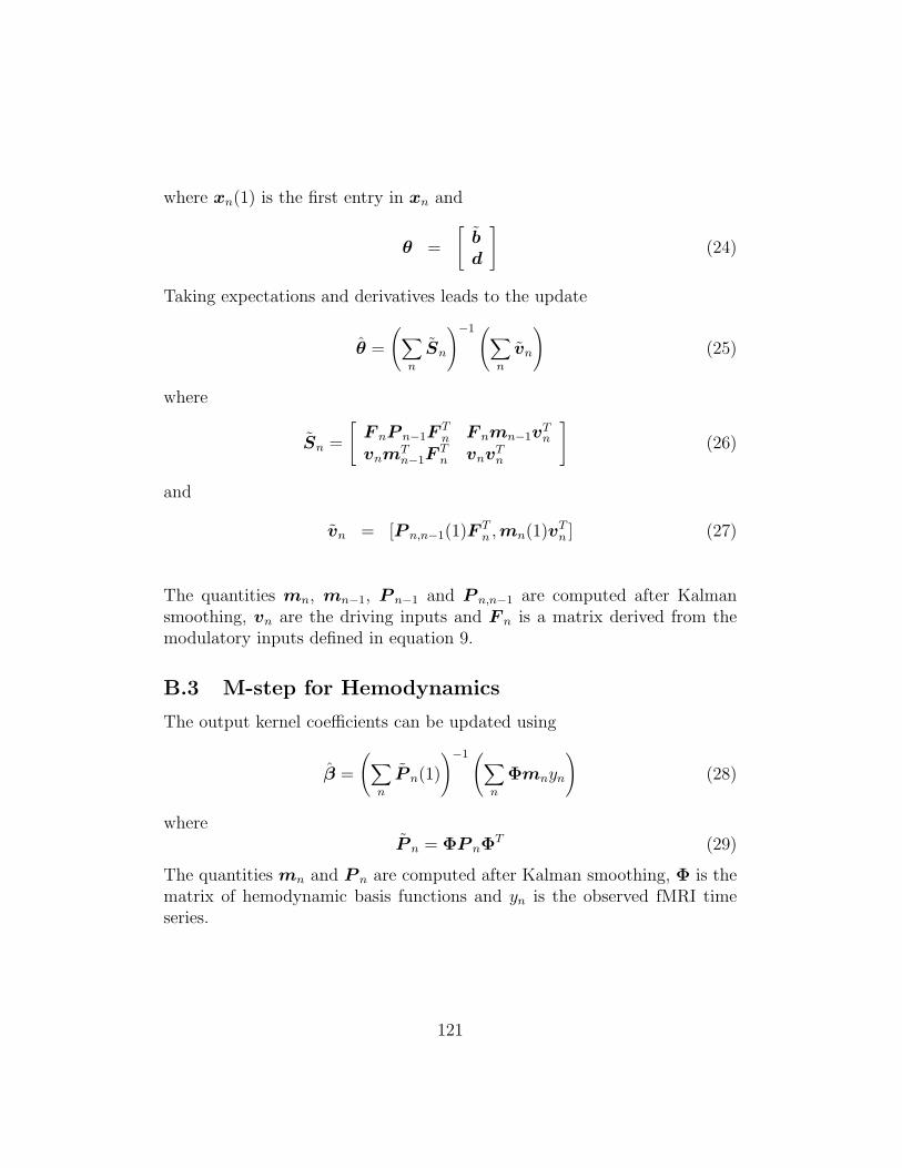
where xn(1) is the first entry in xn and

θ =

[bd

](24)

Taking expectations and derivatives leads to the update

θ =

(∑n

Sn

)−1 (∑n

vn

)(25)

where

Sn =

[F nP n−1F

Tn F nmn−1v

Tn

vnmTn−1F

Tn vnv

Tn

](26)

and

vn = [P n,n−1(1)F Tn , mn(1)vT

n ] (27)

The quantities mn, mn−1, P n−1 and P n,n−1 are computed after Kalmansmoothing, vn are the driving inputs and F n is a matrix derived from themodulatory inputs defined in equation 9.

B.3 M-step for Hemodynamics

The output kernel coefficients can be updated using

β =

(∑n

P n(1)

)−1 (∑n

Φmnyn

)(28)

whereP n = ΦP nΦ

T (29)

The quantities mn and P n are computed after Kalman smoothing, Φ is thematrix of hemodynamic basis functions and yn is the observed fMRI timeseries.

121

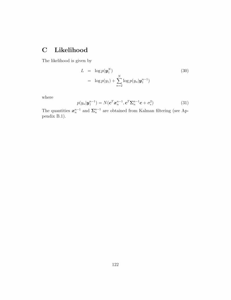
C Likelihood

The likelihood is given by

L = log p(yN1 ) (30)

= log p(y1) +N∑

n=2

log p(yn|yn−11 )

wherep(yn|yn−1

1 ) = N(cT xn−1n , cTΣn−1

n c + σ2e) (31)

The quantities xn−1n and Σn−1

n are obtained from Kalman filtering (see Ap-pendix B.1).

122

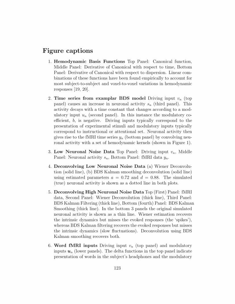
Figure captions

1. Hemodynamic Basis Functions Top Panel: Canonical function,Middle Panel: Derivative of Canonical with respect to time, BottomPanel: Derivative of Canonical with respect to dispersion. Linear com-binations of these functions have been found empirically to account formost subject-to-subject and voxel-to-voxel variations in hemodynamicresponses [19, 20].

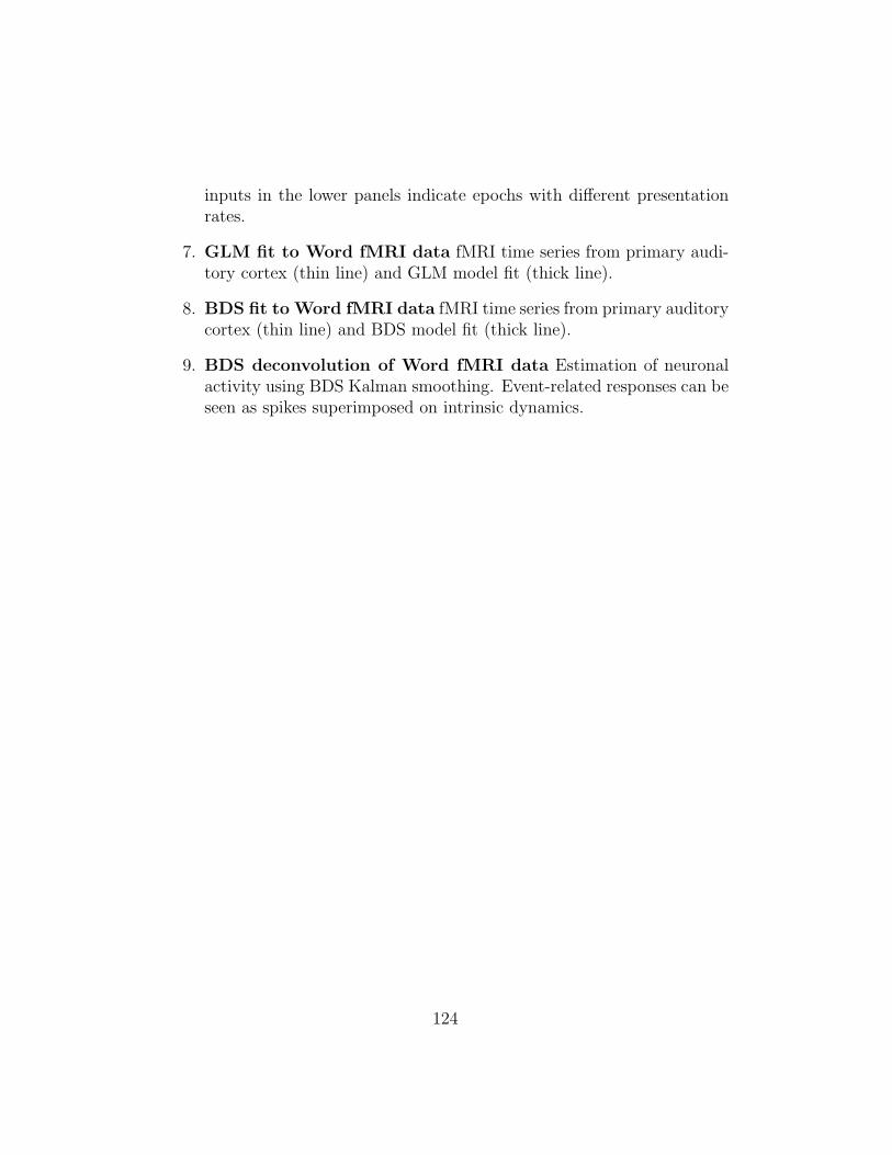
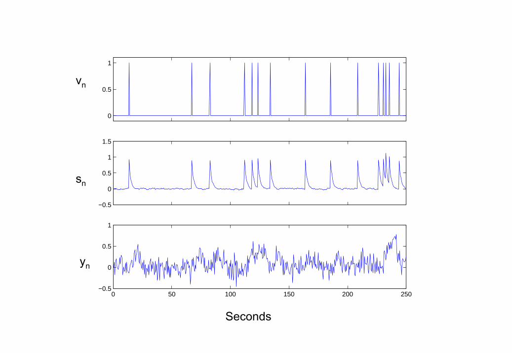
2. Time series from examplar BDS model Driving input vn (toppanel) causes an increase in neuronal activity sn (third panel). Thisactivity decays with a time constant that changes according to a mod-ulatory input un (second panel). In this instance the modulatory co-efficient, b, is negative. Driving inputs typically correspond to thepresentation of experimental stimuli and modulatory inputs typicallycorrespond to instructional or attentional set. Neuronal activity thengives rise to the fMRI time series yn (bottom panel) by convolving neu-ronal activity with a set of hemodynamic kernels (shown in Figure 1).

3. Low Neuronal Noise Data Top Panel: Driving input vn, MiddlePanel: Neuronal activity sn, Bottom Panel: fMRI data yn.

4. Deconvolving Low Neuronal Noise Data (a) Wiener Deconvolu-tion (solid line), (b) BDS Kalman smoothing deconvolution (solid line)using estimated parameters a = 0.72 and d = 0.88. The simulated(true) neuronal activity is shown as a dotted line in both plots.

5. Deconvolving High Neuronal Noise Data Top (First) Panel: fMRIdata, Second Panel: Wiener Deconvolution (thick line), Third Panel:BDS Kalman Filtering (thick line), Bottom (fourth) Panel: BDS KalmanSmoothing (thick line). In the bottom 3 panels the original simulatedneuronal activity is shown as a thin line. Wiener estimation recoversthe intrinsic dynamics but misses the evoked responses (the ‘spikes’),whereas BDS Kalman filtering recovers the evoked responses but missesthe intrinsic dynamics (slow fluctuations). Deconvolution using BDSKalman smoothing recovers both.

6. Word fMRI inputs Driving input vn (top panel) and modulatoryinputs un (lower panels). The delta functions in the top panel indicatepresentation of words in the subject’s headphones and the modulatory

123

inputs in the lower panels indicate epochs with different presentationrates.

7. GLM fit to Word fMRI data fMRI time series from primary audi-tory cortex (thin line) and GLM model fit (thick line).

8. BDS fit to Word fMRI data fMRI time series from primary auditorycortex (thin line) and BDS model fit (thick line).

9. BDS deconvolution of Word fMRI data Estimation of neuronalactivity using BDS Kalman smoothing. Event-related responses can beseen as spikes superimposed on intrinsic dynamics.

124

−0.05

0

0.05

0.1

−0.02

0

0.02

0.04

0 2 4 6 8 10 12 14 16 18 20

−0.05

0

0.05

Seconds

Canonical,

TemporalDerivative,

DispersionDerivative,

φ1

φ3

φ2

0

0.5

1

0

0.5

1

0

0.5

1

0 50 100 150 200 250

0

0.5

1

vn

un

sn

yn

Seconds

0

0.5

1

−0.5

0

0.5

1

1.5

0 50 100 150 200 250−0.5

0

0.5

1

Seconds

vn

sn

yn

0 50 100 150 200 250−0.4

−0.2

0

0.2

0.4

0.6

0.8

1

1.2

Seconds

s n

0 50 100 150 200 250−0.2

0

0.2

0.4

0.6

0.8

1

1.2

Seconds

s n

(a)

(b)

Seconds

fMRI

Wiener

BDS KF

BDS KS

0

0.5

1

0

0.5

1

0

0.5

1

0 50 100 150 200 2500

0.5

1

vn

un(1)

un(2)

un(3)

Seconds

0 50 100 150 200 250−3

−2

−1

0

1

2

3

Seconds

0 50 100 150 200 250−3

−2

−1

0

1

2

3

Seconds

0 50 100 150 200 250−2.5

−2

−1.5

−1

−0.5

0

0.5

1

1.5

2

Seconds