
Networked Timetable Stability Improvement Based on a Bilevel ...

BILEVEL PARAMETER LEARNING FOR HIGHER-ORDER
TOTAL VARIATION REGULARISATION MODELS∗
J.C. DE LOS REYES1, C.-B. SCHONLIEB2 AND T. VALKONEN2
Abstract. We consider a bilevel optimisation approach for parameter learningin higher-order total variation image reconstruction models. Apart from the leastsquares cost functional, naturally used in bilevel learning, we propose and analysean alternative cost, based on a Huber regularised TV-seminorm. Differentiabilityproperties of the solution operator are verified and a first-order optimality systemis derived. Based on the adjoint information, a quasi-Newton algorithm is pro-posed for the numerical solution of the bilevel problems. Numerical experimentsare carried out to show the suitability of our approach and the improved perfor-mance of the new cost functional. Thanks to the bilevel optimisation framework,also a detailed comparison between TGV2 and ICTV is carried out, showing theadvantages and shortcomings of both regularisers, depending on the structure ofthe processed images and their noise level.
1. Introduction
In this paper we propose a bilevel optimisation approach for parameter learning inhigher-order total variation regularisation models for image restoration. The recon-struction of an image from imperfect measurements is essential for all research whichrelies on the analysis and interpretation of image content. Mathematical image re-construction approaches aim to maximise the information gain from acquired imagedata by intelligent modelling and mathematical analysis.
A variational image reconstruction model can be formalised as follows. Given dataf which is related to an image (or to certain image information, e.g. a segmented oredge detected image) u through a generic forward operator (or function) K the taskis to retrieve u from f . In most realistic situations this retrieval is complicated bythe ill-posedness of K as well as random noise in f . A widely accepted method thatapproximates this ill-posed problem by a well-posed one and counteracts the noise isthe method of Tikhonov regularisation. That is, an approximation to the true imageis computed as a minimiser of
(1.1) α R(u) + d(K(u), f),
where R is a regularising energy that models a-priori knowledge about the image u,d(·, ·) is a suitable distance function that models the relation of the data f to theunknown u, and α > 0 is a parameter that balances our trust in the forward model
1Research Center on Mathematical Modelling (MODEMAT), Escuela PolitecnicaNacional, Quito, Ecuador.
2Department of Applied Mathematics and Theoretical Physics, University of Cam-bridge, Cambridge, United Kingdom.
∗This research has been supported by King Abdullah University of Science and Technology(KAUST) Award No. KUK-I1-007-43, EPSRC grants Nr. EP/J009539/1 “Sparse & Higher-orderImage Restoration” and Nr. EP/M00483X/1 “Efficient computational tools for inverse imaging prob-lems”, Escuela Politecnica Nacional de Quito Award No. PIS 12-14 and MATHAmSud projectSOCDE “Sparse Optimal Control of Differential Equations”. While in Quito, T. Valkonen has more-over been supported by SENESCYT (Ecuadorian Ministry of Higher Education, Science, Technologyand Innovation) under a Prometeo Fellowship.
1
2 OPTIMAL HIGHER-ORDER TOTAL VARIATION REGULARISATION
against the need of regularisation. The parameter α in particular, depends on theamount of ill-posedness in the operator K and the amount (amplitude) of the noisepresent in f . A key issue in imaging inverse problems is the correct choice of α, imagepriors (regularisation functionals R), fidelity terms d and (if applicable) the choiceof what to measure (the linear or nonlinear operator K). Depending on this choice,different reconstruction results are obtained.
While functional modelling (1.1) constitutes a mathematically rigorous and phys-ical way of setting up the reconstruction of an image – providing reconstructionguarantees in terms of error and stability estimates – it is limited with respect to itsadaptivity for real data. On the other hand, data-based modelling of reconstructionapproaches is set up to produce results which are optimal with respect to the givendata. However, in general it neither offers insights into the structural properties ofthe model nor provides comprehensible reconstruction guarantees. Indeed, we believethat for the development of reliable, comprehensible and at the same time effectivemodels (1.1) it is essential to aim for a unified approach that seeks tailor-made regu-larisation and data models by combining model- and data-based approaches.
To do so we focus on a bilevel optimisation strategy for finding an optimal setupof variational regularisation models (1.1). That is, for a given training pair of noisyand original clean images (f, f0), respectively, we consider a learning problem of theform
(1.2) minF (u∗) = cost(u∗, f0) subject to u∗ ∈ arg minu
α R(u) + d(K(u), f) ,
where F is a generic cost functional that measures the fitness of u∗ to the original im-age f0. The argument of the minimisation problem will depend on the specific setup(i.e. the degrees of freedom) in the constraint problem (1.1). In particular, we pro-pose a bilevel optimisation approach for learning optimal parameters in higher-ordertotal variation regularisation models for image reconstruction in which the argumentsof the optimisation constitute parameters in front of the first- and higher-order regu-larisation terms. Rather than working on the discrete problem, as is done in standardparameter learning and model optimisation methods, we optimise the regularisationmodels in infinite dimensional function space. We will explain this approach in moredetail in the next section. Before, let us give an account to the state of the art ofbilevel optimisation for model learning. In machine learning bilevel optimisation iswell established. It is a semi-supervised learning method that optimally adapts itselfto a given dataset of measurements and desirable solutions. In [34, 18, 14], for in-stance the authors consider bilevel optimization for finite dimensional Markov randomfield models. In inverse problems the optimal inversion and experimental acquisitionsetup is discussed in the context of optimal model design in works by Haber, Horeshand Tenorio [21, 20], as well as Ghattas et al. [8, 3]. Recently parameter learningin the context of functional variational regularisation models (1.1) also entered theimage processing community with works by the authors [16, 9], Kunisch, Pock andco-workers [26, 13], Chung et al. [15] and Hintermuller et al. [24].
Apart from the work of the authors [16, 9], all approaches so far are formulatedand optimised in the discrete setting. Our subsequent modelling, analysis and opti-misation will be carried out in function space rather than on a discretisation of (1.1).While digitally acquired image data is of course discrete, the aim of high resolutionimage reconstruction and processing is always to compute an image that is close tothe real (analogue, infinite dimensional) world. Hence, it makes sense to seek imageswhich have certain properties in an infinite dimensional function space. That is, weaim for a processing method that accentuates and preserves qualitative properties inimages independent of the resolution of the image itself [36]. Moreover, optimisation
OPTIMAL HIGHER-ORDER TOTAL VARIATION REGULARISATION 3
methods conceived in function space potentially result in numerical iterative schemeswhich are resolution and mesh-independent upon discretisation [23].
Higher-order total variation regularisation has been introduced as an extension ofthe standard total variation regulariser in image processing. As the Total Variation(TV) [32] and many more contributions in the image processing community haveproven, a non-smooth first-order regularisation procedure results in a nonlinear smooth-ing of the image, smoothing more in homogeneous areas of the image domain andpreserving characteristic structures such as edges. In particular, the TV regulariser istuned towards the preservation of edges and performs very well if the reconstructedimage is piecewise constant. The drawback of such a regularisation procedure becomesapparent as soon as images or signals (in 1D) are considered which do not only con-sist of constant regions and jumps, but also possess more complicated, higher-orderstructures, e.g. piecewise linear parts. The artefact introduced by TV regularisationin this case is called staircasing [31]. One possibility to counteract such artefacts isthe introduction of higher-order derivatives in the image regularisation. Chambolleand Lions [10], for instance, propose a higher order method by means of an infimalconvolution of the TV and the TV of the image gradient called Infimal-ConvolutionTotal Variation (ICTV) model. Other approaches to combine first and second orderregularisation originate, for instance, from Chan, Marquina, and Mulet [11] who con-sider total variation minimisation together with weighted versions of the Laplacian,the Euler-elastica functional [29, 12] which combines total variation regularizationwith curvature penalisation, and many more [27, 30] just to name a few. RecentlyBredies et al. have proposed Total Generalized Variation (TGV) [5] as a higher-ordervariant of TV regularisation.
In this work we mainly concentrate on two second-order total variation models:the recently proposed TGV [5] and the ICTV model of Chambolle and Lions [10].We focus on second-order TV regularisation only since this is the one which seems tobe most relevant in imaging applications [25, 4]. For Ω ⊂ R2 open and bounded andu ∈ BV (Ω), the ICTV regulariser reads
(1.3) ICTVα,β(u) := minv∈W 1,1(Ω), ∇v∈BV (Ω)
α‖Du−∇v‖M(Ω;R2) + β‖D∇v‖M(Ω;R2×2).
On the other hand, second-order TGV [7, 6] for u ∈ BV (Ω) reads
(1.4) TGV2α,β(u) := min
w∈BD(Ω)α‖Du− w‖M(Ω;R2) + β‖Ew‖M(Ω;Sym2(R2)).
Here BD(Ω) := w ∈ L1(Ω;Rn) | ‖Ew‖M(Ω;Rn×n) < ∞ is the space of vector fields
of bounded deformation on Ω, E denotes the symmetrised gradient and Sym2(R2) thespace of symmetric tensors of order 2 with arguments in R2. The parameters α, β arefixed positive parameters and will constitute the arguments in the special learningproblem a la (1.2) we consider in this paper. The main difference between (1.3) and(1.4) is that we do not generally have that w = ∇v for any function v. That results insome qualitative differences of ICTV and TGV regularisation, compare for instance[1]. Substituting αR(u) in (1.1) by TGV2
α,β(u) or ICTVα,β(u) gives the TGV imagereconstruction model and the ICTV image reconstruction model, respectively. In thispaper we only consider the case K = Id identity and d(u, f) = ‖u− f‖2L2(Ω) in (1.1)
which corresponds to an image de-noising model for removing Gaussian noise. Withour choice of regulariser the former scalar α in (1.1) has been replaced by a vector(α, β) of two parameters in (1.4) and (1.3). The choice of the entries in this vectornow do not only determine the overall strength of the regularisation (depending onthe properties of K and the noise level) but those parameters also balance betweenthe different orders of regularity of the function u, and their choice is indeed crucialfor the image reconstruction result. Large β will give regularised solutions that are
4 OPTIMAL HIGHER-ORDER TOTAL VARIATION REGULARISATION
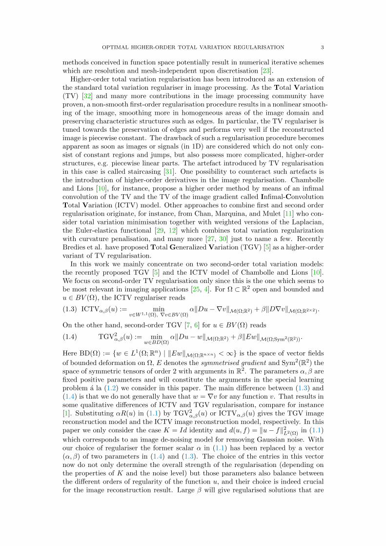
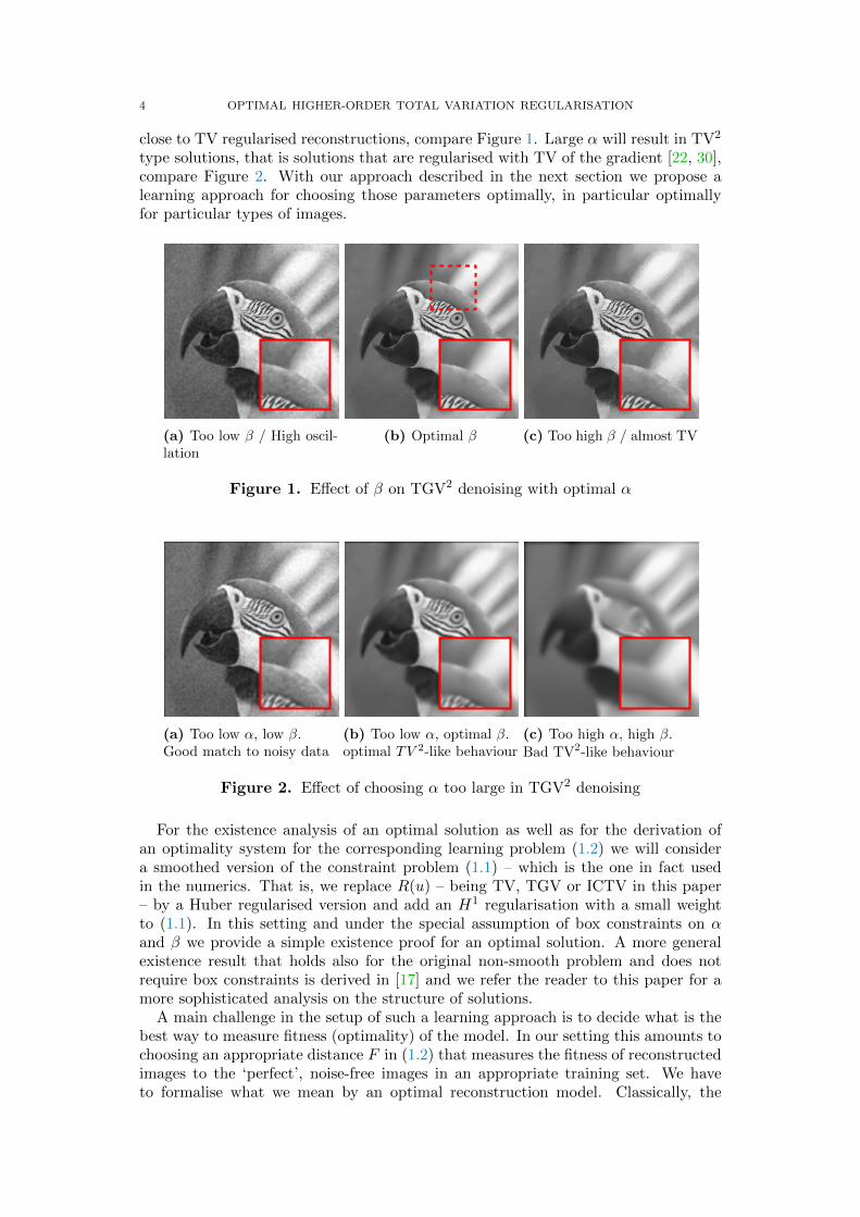
close to TV regularised reconstructions, compare Figure 1. Large α will result in TV2
type solutions, that is solutions that are regularised with TV of the gradient [22, 30],compare Figure 2. With our approach described in the next section we propose alearning approach for choosing those parameters optimally, in particular optimallyfor particular types of images.
(a) Too low β / High oscil-lation
(b) Optimal β (c) Too high β / almost TV
Figure 1. Effect of β on TGV2 denoising with optimal α
(a) Too low α, low β.Good match to noisy data
(b) Too low α, optimal β.optimal TV 2-like behaviour
(c) Too high α, high β.Bad TV2-like behaviour
Figure 2. Effect of choosing α too large in TGV2 denoising
For the existence analysis of an optimal solution as well as for the derivation ofan optimality system for the corresponding learning problem (1.2) we will considera smoothed version of the constraint problem (1.1) – which is the one in fact usedin the numerics. That is, we replace R(u) – being TV, TGV or ICTV in this paper– by a Huber regularised version and add an H1 regularisation with a small weightto (1.1). In this setting and under the special assumption of box constraints on αand β we provide a simple existence proof for an optimal solution. A more generalexistence result that holds also for the original non-smooth problem and does notrequire box constraints is derived in [17] and we refer the reader to this paper for amore sophisticated analysis on the structure of solutions.
A main challenge in the setup of such a learning approach is to decide what is thebest way to measure fitness (optimality) of the model. In our setting this amounts tochoosing an appropriate distance F in (1.2) that measures the fitness of reconstructedimages to the ‘perfect’, noise-free images in an appropriate training set. We haveto formalise what we mean by an optimal reconstruction model. Classically, the

OPTIMAL HIGHER-ORDER TOTAL VARIATION REGULARISATION 5
difference between the original, noise-free image f0 and its regularised version uα,β iscomputed with an L2
2 cost functional
(1.5) FL22(uα,β) = ‖uα,β − f0‖2L2(Ω),
which is closely related to the PSNR quality measure. Apart from this, we proposein this paper an alternative cost functional based on a Huberised total variation cost
(1.6) FL1η∇(uα,β) :=
∫Ω|D(uα,β − f0)|γ dx,
where the Huber regularisation | · |γ will be defined later on in Definition 2.1. Wewill see that the choice of this cost functional is indeed crucial for the qualitativeproperties of the reconstructed image.
The proposed bilevel approach has an important indirect consequence: It estab-lishes a basis for the comparison of the different total variation regularisers employedin image denoising tasks. In the last part of the paper we exhaustively compare theperformance of TV, TGV2 and ICTV for various image datasets. The parameters arechosen optimally, according to the proposed bilevel approach, and different qualitymeasures (like PSNR and SSIM) are considered for the comparison. The obtainedresults are enlightening about when to use each one of the considered regularisers. Inparticular, ICTV appears to behave better for images with arbitrary structure andmoderate noise levels, whereas TGV2 behaves better for images with large smoothareas.
Outline of the paper In Section 2 we state the bilevel learning problem for thetwo higher-order total variation regularisation models, TGV and ICTV, and proveexistence of an optimal parameter pair α, β. The bilevel optimization problem is anal-ysed in Section 3, where existence of Lagrange multipliers is proved and an optimalitysystem, as well as a gradient formula, are derived. Based on the optimality condition,a BFGS algorithm for the bilevel learning problem is devised in Section 5.1. Forthe numerical solution of each denoising problem an infeasible semi-smooth Newtonmethod is considered. Finally, we discuss the performance of the parameter learningmethod by means of several examples for the denoising of natural photographs inSection 5. Therein, we also present a statistical analysis on how TV, ICTV and TGVregularisation compare in terms of returned image quality, carried out on 200 imagesfrom the Berkeley segmentation dataset BSDS300.
2. Problem statement and existence analysis
We strive to develop a parameter learning method for higher-order total variationregularisation models that maximises the fit of the reconstructed images to trainingimages simulated for an application at hand. For a given noisy image f ∈ L2(Ω),Ω ⊂ R2 open and bounded, we consider
(2.1) minu
Rα,β(u) +
1
2‖u− f‖2L2(Ω)
.
where, α, β ∈ R. We focus on TGV2 and ICTV image denoising:
Rα,β(u) = TGV2α,β(u) := min
w∈BD(Ω)‖α (Du− w)‖M(Ω;R2)
+ ‖β Ew‖M(Ω;Sym2(R2)).
6 OPTIMAL HIGHER-ORDER TOTAL VARIATION REGULARISATION
and (1.3) with spatial dependence
Rα,β(u) = ICTVα,β(u) := minv∈W 1,1(Ω)∇v∈BV (Ω)
‖α (Du−∇v)‖M(Ω;R2)
+ ‖β D∇v‖M(Ω;R2×2),
for u ∈ BV (Ω). For this model, we want to determine the optimal choice of α, β,given a particular type of images and a fixed noise level. More precisely, we consider atraining pair (f, f0), where f is a noisy image corrupted by normally distributed noisewith a fixed variation, and the image f0 represents the ground truth or an image thatapproximates the ground truth within a desirable tolerance. Then, we determine theoptimal choice of α, β by solving the following problem
(2.2) min(α,β)∈R2
F (uα,β) s.t. α, β ≥ 0,
where F equals the L22 cost (1.5) or the Huberised TV cost (1.6) and uα,β for a given
f solves a regularised version of the minimization problem (2.1) that will be specifiedin the next section, compare problem (2.3b). This regularisation of the problem isa technical requirement for solving the bilevel problem that will be discussed in thesequel. In contrast to learning α, β in (2.1) in finite dimensional parameter spaces (asis the case in machine learning) we aim for novel optimisation techniques in infinitedimensional function spaces.
2.1. Formal statement. Let Ω ⊂ Rn be an open bounded domain with Lipschitzboundary. This will be our image domain. Usually Ω = (0, w) × (0, h) for w and hthe width and height of a two-dimensional image, although no such assumptions aremade in this work. Our data f and f0 are assumed to lie in L2(Ω).
In our learning problem, we look for parameters (α, β) that for some cost functionalF : H1(Ω)→ R solve the problem
(2.3a) min(α,β)∈R2
F (uα,β)
subject to
uα,β ∈ arg minu∈H1(Ω)
Jγ,µ(u;α, β)(2.3b)
α, β ≥ 0,(2.3c)
where
Jγ,µ(u;α, β) :=1
2‖u− f‖2L2(Ω) +Rγ,µα,β(u).
Here Jγ,µ(·;α, β) is the regularised denoising functional that amends the regularisa-tion term in (2.1) by a Huber regularised version of it with parameter γ > 0, and anelliptic regularisation term with parameter µ > 0. In the case of TGV2 the modifiedregularisation term Rγ,µα,β(u) then reads for u ∈ H1(Ω)
TGV2,γ,µα,β (u) := min
w∈H1(Ω)
∫Ωα |Du− w|γ dx
+
∫Ωβ |Ew|γ dx+
µ
2
(‖u‖2H1(Ω) + ‖w‖2H1(Ω)
)
OPTIMAL HIGHER-ORDER TOTAL VARIATION REGULARISATION 7
and in the case of ICTV we have
ICTVγ,µα,β(u) := min
v∈W 1,1(Ω)∇v∈BV (Ω,Rn)∩H1(Ω)
∫Ωα |Du−∇v|γ dx
+
∫Ωβ |D∇v|γ dx+
µ
2
(‖u‖2H1(Ω) + ‖∇v‖2H1(Ω)
).
Here, H1(Ω) = H1(Ω;Rn) and the Huber regularisation | · |γ is defined as follows.
Definition 2.1. Given γ ∈ (0,∞], we define for the norm ‖ · ‖2 on Rm, the Huberregularisation
|g|γ =
‖g‖2 − 1
2γ , ‖g‖2 ≥ 1/γ,γ2‖g‖
22, ‖g‖2 < 1/γ.
For the cost functional F , given noise-free data f0 ∈ L2(Ω) and a regularisedsolution u ∈ H1(Ω), we consider in particular the L2 cost
FL22(u) :=
1
2‖f0 − u‖2L2(Ω;Rd),
as well as the Huberised total variation cost
FL1η∇(u) :=
∫Ω|D(f0 − u)|γ dx
with noise-free data f0 ∈ BV(Ω).
2.2. Existence of an optimal solution. The existence of an optimal solution forthe learning problem (2.3) is a special case of the class of bilevel problems considered in[17], where existence of optimal parameters in (0,+∞]2N is proven. For convenience,we provide a simplified proof for the case where box constraints on the parametersare imposed. We start with an auxiliary lower semicontinuity result for the Huberregularised functionals.
Lemma 2.1. Let u, v ∈ Lp(Ω), 1 ≤ p <∞. Then, the functional u 7→∫
Ω |u− v|γ dx,where | · |γ is the Huber regularisation in Definition 2.1, is lower semicontinuous with
respect to weak* convergence in M(Ω;Rd)
Proof. Recall that for g ∈ Rm, the Huber-regularised norm may be written in dualform as
|g|γ = sup〈q, g〉 − γ
2‖q‖22 : ‖q‖2 ≤ 1
.
Therefore, we find that
G(u) :=
∫Ω|u− v|γ dx = sup
∫Ωu(x) · ϕ(x) dx−
∫Ω
γ
2‖ϕ(x)‖22 dx :
ϕ ∈ C∞c (Ω), ‖ϕ(x)‖2 ≤ α for every x ∈ Ω.
The functional G is of the form G(u) = sup〈u, ϕ〉 −G∗(ϕ), where G∗ is the convexconjugate of G. Now, let ui∞i=1 converge to u weakly* in M(Ω;Rd). Taking asupremising sequence ϕj∞j=1 for this functional at any point u, we easily see lower
semicontinuity by considering the sequences 〈ui, ϕj〉 −G∗(ϕj)∞i=1 for each j.
Our main existence result is the following.

8 OPTIMAL HIGHER-ORDER TOTAL VARIATION REGULARISATION
Theorem 2.1. We consider the learning problem (2.3) for TGV2 and ICTV regu-larisation, optimising over parameters (α, β) such that 0 ≤ α ≤ α, 0 ≤ β ≤ β. Here(α, β) <∞ is an arbitrary but fixed vector in R2 that defines a box constraint on the
parameter space. Then, there exists an optimal solution (α, β) ∈ R2 for this problemfor both choices of cost functionals, F = L2
2 and F = FL1η∇.
Proof. Let (αn, βn) ⊂ R2 be a minimising sequence. Due to the box constraintswe have that the sequence (αn, βn) is bounded in R2. Moreover, we get for thecorresponding sequences of states un := u(αn,βn) that
Jγ,µ(un;αn, βn) ≤ Jγ,µ(u;αn, βn), ∀u ∈ H1(Ω),
in particular this holds for u = 0. Hence,
(2.4)1
2‖un − f‖2L2(Ω) +Rγ,µαn,βn(un) ≤ 1
2‖f‖2L2(Ω).
Exemplarily, we consider here the case for the TGV regulariser, that is Rγ,µαn,βn =
TGV2,γ,µα,β . The proof for the ICTV regulariser can be done in a similar fashion.
Inequality (2.4) in particular gives
‖un‖2H1(Ω) + ‖wn‖2H1(Ω) ≤1
µ‖f‖L2(Ω),
where wn is the optimal w for un. This gives that (un, wn) is uniformly bounded inH1(Ω)×H1(Ω) and that there exists a subsequence (αn, βn, un, wn) which converges
weakly in R2×H1(Ω)×H1(Ω) to a limit point (α, β, u, w). Moreover, un → u stronglyin Lp(Ω) and wn → w in Lp(Ω;Rn). Using the continuity of the L2 fidelity term withrespect to strong convergence in L2, and the weak lower semicontinuity of the H1
term with respect to weak convergence in H1 and of the Huber regularised functionaleven with respect to weak∗ convergence in M (cf. Lemma 2.1) we get
1
2‖u− f‖2L2(Ω) +
∫Ωα |Du− w|γ dx+
∫Ωβ |Ew|γ dx
+µ
2
(‖u‖2H1(Ω) + ‖w‖2H1(Ω)
)≤ lim inf
n
1
2‖un − f‖2L2(Ω) +
∫Ωα |Dun − wn|γ dx+
∫Ωβ |Ewn|γ dx
+µ
2
(‖un‖2H1(Ω) + ‖wn‖2H1(Ω)
)≤ lim inf
n
1
2‖un − f‖2L2(Ω) +
∫Ωαn |Dun − wn|γ dx+
∫Ωβn |Ewn|γ dx
+µ
2
(‖un‖2H1(Ω) + ‖wn‖2H1(Ω)
),
where in the last step we have used the boundedness of the sequence Rγ,µαn,βn(un) from
(2.4) and the convergence of (αn, βn) in R2. This shows that the limit point u is an
optimal solution for (α, β). Moreover, due to the weak lower semicontinuity of thecost functional F and the fact that the set (α, β) : 0 ≤ α ≤ α, 0 ≤ β ≤ β is closed,
we have that (α, β, u) is optimal for (2.3).
Remark 2.1.
• Using the existence result in [17], in principle we could allow infinite values forα and β. This would include both TV2 and TV as possible optimal regularisersin our learning problem.
OPTIMAL HIGHER-ORDER TOTAL VARIATION REGULARISATION 9
• In [17], in the case of the L2 cost and assuming that
Rγα,β(f) > Rγα,β(f0),
we moreover show that the parameters (α, β) are strictly larger than 0. Inthe case of the Huberised TV cost this can only be proven in a discretisedsetting. Please see [17] for details.• The existence of solutions with µ = 0, that is without elliptic regularisation,
is also proven in [17]. Note that here, we focus on the µ > 0 case since theelliptic regularity is required for proving the existence of Lagrange multipliersin the next section.
3. Lagrange multipliers
In this section we prove the existence of Lagrange multipliers for the learning prob-lem (2.3) and derive an optimality system that characterizes its solution. Moreover,a gradient formula for the reduced cost functional is obtained, which plays an im-portant role in the development of fast solution algorithms for the learning problems(see Section 5.1).
In what follows all proofs are presented for the TGV2 regularisation case, that isRγα,β = TGV2,γ
α,β. However, possible modifications to cope with the ICTV model will
also be commented.We start by investigating the differentiability of the solution operator.
3.1. Differentiability of the solution operator. We recall that the TGV2 denois-ing problem is given by
u = (v, w) = arg minBV×BD
1
2
∫Ω|v − f |2 +
∫Ωα|Dv − w|γ +
∫Ωβ|Ew|γ
.
Using an elliptic regularization we then get
u = arg minH1(Ω)×H1(Ω)
a(u, u) +
1
2
∫Ω|v − f |2 +
∫Ωα|Dv − w|γ +
∫Ωβ|Ew|γ
,
where a(u, u) = µ(‖v‖2H1 + ‖w‖2H1
). A necessary and sufficient optimality condition
for the latter is then given by the following variational equation
(3.1) a(u,Ψ) +
∫Ωαhγ(Dv − w)(Dφ− ϕ) dx
+
∫Ωβhγ(Ew)Eϕdx+
∫Ω
(v − f)φdx = 0, for all Ψ ∈ U,
where Ψ = (φ, ϕ) and U = H1(Ω)×H1(Ω).
Theorem 3.1. The solution operator S : R2 7→ U , which assigns to each pair (α, β) ∈R2 the corresponding solution to the denoising problem (3.1), is Frechet differentiableand its derivative is characterized by the unique solution z = S′(α, β)[θ1, θ2] ∈ U ofthe following linearized equation:
(3.2) a(z,Ψ) +
∫Ωθ1 hγ(Dv − w)(Dφ− ϕ) dx
+
∫Ωαh′γ(Dv − w)(Dz1 − z2)(Dφ− ϕ) dx+
∫Ωθ2 hγ(Ew)Eϕdx
+
∫Ωβh′γ(Ew)Ez2Eϕdx+
∫Ωz1φdx = 0, for all Ψ ∈ U.
10 OPTIMAL HIGHER-ORDER TOTAL VARIATION REGULARISATION
Proof. Thanks to the ellipticity of a(·, ·) and the monotonicity of hγ , existence of aunique solution to the linearized equation follows from the Lax-Milgram theorem.
Let ξ := u+ − u− z, where u = S(α, β) and u+ = S(α+ θ1, β + θ2). Our aim is toprove that ‖ξ‖U = o(|θ|). Combining the equations for u+, u and z we get that
a(ξ,Ψ) +
∫Ω
(α+ θ1) hγ(Dv+ − w+)(Dφ− ϕ) dx−∫
Ωα hγ(Dv − w)(Dφ− ϕ) dx
−∫
Ωθ1 hγ(Dv − w)(Dφ− ϕ) dx−
∫Ωαh′γ(Dv − w)(Dz1 − z2)(Dφ− ϕ) dx
+
∫Ω
(β + θ2)hγ(Ew+)Eϕdx−∫
Ωβhγ(Ew)Eϕdx
−∫
Ωθ2 hγ(Ew)Eϕdx−
∫Ωβ h′γ(Ew)Ez2Eϕdx+ 2
∫Ωξ1φdx = 0, for all Ψ ∈ U,
where ξ := (ξ1, ξ2) ∈ H1(Ω)×H1(Ω). Adding and subtracting the terms∫Ωαh′γ(Dv − w)(Dδv − δw)(Dφ− ϕ) dx
and ∫Ωβh′γ(Ew)Eδw : Eϕdx,
where δv := vα+θ − v and δw := wα+θ − w, we obtain that
a(ξ,Ψ) +
∫Ωαh′γ(Dv − w)(Dξ1 − ξ2)(Dφ− ϕ)
+
∫Ωβh′γ(Ew)Eξ2 : Eϕdx+ 2
∫Ωξ1φdx
= −∫
Ωα[hγ(Dv+ − w+)− hγ(Dv − w)− h′γ(Dv − w)(Dδv − δw)
](Dφ− ϕ)
−∫
Ωθ1
[hγ(Dv+ − w+)− hγ(Dv − w)
](Dφ− ϕ) dx
−∫
Ωβ[hγ(Ew+)− hγ(Ew)− h′γ(Ew)Eδw
]: Eϕdx
−∫
Ωθ2 [hγ(Ewα+θ)− hγ(Ew)] : Eϕdx, for all Ψ ∈ U.
Testing with Ψ = ξ and using the monotonicity of h′γ(·) we get that
‖ξ‖U ≤ C|α|∥∥hγ(Dv+ − w+)− hγ(Dv − w)− h′γ(Dv − w)(Dδv − δw)
∥∥L2
+ |θ1|∥∥hγ(Dv+ − w+)− hγ(Dv − w)
∥∥L2
+|β|∥∥hγ(Ew+)− hγ(Ew)− h′γ(Ew)Eδw
∥∥L2
+|θ2| ‖hγ(Ewα+θ)− hγ(Ew)‖L2
,
for some generic constant C > 0. Considering the differentiability and Lipschitzcontinuity of h′γ(·), it then follows that
(3.3) ‖ξ‖U ≤ C(|α| o(
∥∥u+ − u∥∥
1,p) + |θ1| ‖uα+θ − u‖U
+ |β| o(∥∥w+ − w
∥∥1,p
) + |θ2| ‖wα+θ − w‖H1(Ω)
),
OPTIMAL HIGHER-ORDER TOTAL VARIATION REGULARISATION 11
where ‖ · ‖1,p stands for the norm in the space W1,p(Ω). From regularity results forsecond order systems (see [19, Thm. 1, Rem. 14]), it follows that∥∥u+ − u
∥∥1,p≤ L|θ| (‖Div hγ(Dv − w)‖−1,p + ‖hγ(Dv − w)‖−1,p + ‖Div hγ(Ew)‖−1,p)
≤ L|θ| (2‖hγ(Dv − w)‖L∞ + ‖hγ(Ew)‖L∞)
≤ L|θ|,
since |hγ(·)| ≤ 1. Inserting the latter in estimate (3.3), we finally get that
‖ξ‖U = o(|θ|).
Remark 3.1. The Frechet differentiability proof makes use of the quasilinear struc-ture of the TGV2 variational form, making it difficult to extend to the ICTV modelwithout further regularisation terms. For the latter, however, a Gateaux differentia-bility result may be obtained using the same proof technique as in [16].
3.2. The adjoint equation. Next, we use the Lagrangian formalism for deriving theadjoint equations for both the TGV2 and ICTV learning problems. Existence of asolution to the adjoint equation then follows from the well-posedness of the linearizedequation.
Defining the Lagrangian associated to TGV2 learning problem by:
L(v, w, α, β, p1, p2) = F (u) + µ(v, p1)H1 + µ(w, p2)H1
+
∫Ωαhγ(Dv − w)(Dp1 − p2) +
∫Ωβhγ(Ew)Ep2 +
∫Ω
(v − f)p1,
and taking the derivative with respect to the state variable (v, w), we get the necessaryoptimality condition
L′(u,v)(u, v, α, β, p1, p2)[(δv, δw)] = F ′(u)δu + µ(p1, δv)H1 + µ(p2, δw)H1
+
∫Ωαh′γ(Dv − w)(Dδv − δw)(Dp1 − p2)
+
∫Ωβh′γ(Ew)EδwEp2 +
∫Ωp1δv = 0.
If δw = 0, then
µ(p1, δv)H1 +
∫Ωαh′γ(Dv − w)(Dp1 − p2)Dδv +
∫Ωp1δv = −∇vF (u)δv,
whereas if δv = 0, then
µ(p2, δw)H1 −∫
Ωαh′γ(Dv − w)(Dp1 − p2)δw
+
∫Ωβh′γ(Ew) Ep2 Eδw = −∇wF (u)δw.
Existence of a unique solution then follows from the transposition method, sincethe linearised equation is well-posed.
Remark 3.2. For the ICTV model it is possible to proceed formally with the La-grangian approach. We recall that a necessary and sufficient optimality condition for
12 OPTIMAL HIGHER-ORDER TOTAL VARIATION REGULARISATION
the ICTV functional is given by
(3.4) µ(u, φ)H1 + µ(∇v,∇ϕ)H1 +
∫Ωαhγ(Du−∇v)(Dφ−∇ϕ)
+
∫Ωβhγ(D∇v)D∇ϕ+
∫Ω
(u− f)φ = 0, for all (φ, ϕ) ∈ H1(Ω)×H1(Ω)
and the correspondent Lagrangian functional L is given by
L(u, v, α, β, p1, p2) = F (u) + µ(u, p1)H1 + µ(∇v,∇p2)H1
+
∫Ωαhγ(Du−∇v)(Dp1 −∇p2) +
∫Ωβhγ(D∇v)D∇p2 +
∫Ω
(u− f)p1.
Deriving the Lagrangian with respect to the state variable (u, v) and setting it equalto zero yields
L′(u,v)(u, v, α, β, p1, p2)[(δu, δv)] = F ′(u)δu + µ(p1, δu)H1 + µ(∇p2,∇δv)H1
+
∫Ωαh′γ(Du−∇v)(Dδu −∇δv)(Dp1 −∇p2)
+
∫Ωβh′γ(D∇v)D∇δvD∇p2 +
∫Ωp1δu = 0.
By taking succesively δv = 0 and δu = 0, the following system is obtained
(3.5a) µ(p1, δu)H1 +
∫Ωαh′γ(Du − ∇v)(Dp1 − ∇p2)Dδu +
∫Ωp1δu = −F ′(u)δu.
(3.5b) µ(∇p2,∇δv)H1 +
∫Ωαh′γ(Du−∇v)(Dp1 −∇p2)∇δv
+
∫Ωβh′γ(D∇v)D∇p2D∇δv = 0.
3.3. Optimality condition. Using the differentiability of the solution operator andthe well-posedness of the adjoint equation, we derive next an optimality system forthe characterization of local minima of the bilevel learning problem. Besides the opti-mality condition itself, a gradient formula arises as byproduct, which is of importancein the design of solution algorithms for the learning problems.
Theorem 3.2. Let (α, β) ∈ R2+ be a local optimal solution for problem (2.3). Then
there exist Lagrange multipliers Π ∈ U and λ1, λ2 ∈ L2(Ω) such that the followingsystem holds:
(3.6a) a(u,Ψ) + α
∫Ωhγ(Dv − w)(Dφ− ϕ) dx
+ β
∫Ωhγ(Ew)Eϕdx+ 2
∫Ω
(v − f)φdx = 0, for all Ψ ∈ H1(Ω)×H1(Ω),
(3.6b) a(Π,Ψ) + α
∫Ωh′γ(Dv − w)(Dp1 − p2)(Dφ− ϕ) dx
+β
∫Ωh′γ(Ew) Ep2 Eϕdx+2
∫Ωp1φdx = −Fu(u)[Ψ], for all Ψ ∈ H1(Ω)×H1(Ω),
(3.6c) λ1 =
∫Ωhγ(Dv − w)(Dp1 − p2)
OPTIMAL HIGHER-ORDER TOTAL VARIATION REGULARISATION 13
(3.6d) λ2 =
∫Ωhγ(Ew) Ep2
(3.6e) λ1 ≥ 0, λ2 ≥ 0
(3.6f) λ1 · α = λ2 · β = 0.
Proof. Consider the reduced cost functional F(α, β) = F (u(α, β)). The bilevel opti-mization problem can then be formulated as
min(α,β)∈C
F(α, β),
where F : R2 → R and C corresponds to the positive orthant in R2. From [38,Thm. 3.1], there exist multipliers λ1, λ2 such that
λ1 = ∇αF(α, β)
λ2 = ∇βF(α, β)
λ1 ≥ 0, λ2 ≥ 0
λ1 · α = λ2 · β = 0,
By taking the derivative with respect to (α, β) and denoting by u′ the solution tothe linearized equation (3.2) we get, together with the adjoint equation (3.6b), that
F ′(α, β)[φ] = Fu(u)u′(α, β)[φ]
= −a(Π, u′)− α∫
Ωh′γ(Dv − w)(Dp1 − p2)(Dv′ − w′)
− β∫
Ωh′γ(Ew)Ep2 Ew
′ − 2
∫Ωp1v′
= −a(u′,Π)− α∫
Ωh′γ(Dv − w)(Dv′ − w′)(Dp1 − p2)
− β∫
Ωh′γ(Ew)Ew′ Ep2 − 2
∫Ωv′p1
which, taking into account the linearized equation, yields
(3.7) F ′(α, β)[φ] = φ1
∫Ωhγ(Dv − w)(Dp1 − p2) + φ2
∫Ωhγ(Ew)Ep2.
Altogether we proved the result.
Remark 3.3. From the existence result (see Remark 2.1), we actually know that,under some assumptions, α and β are strictly greater than zero. This implies thatthe multipliers λ1 = λ2 = 0 and the problem is of unconstrained nature. This playsan important role in the design of solution algorithms, since only a mild treatment ofthe constraints has to be taken into account, as will be showed in Section 6.
4. Numerical algorithms
In this section we propose a second order quasi-Newton method for the solution ofthe learning problem with scalar regularisation parameters. The algorithm is basedon a BFGS update, preserving the positivity of the iterates through the line searchstrategy and updating the matrix cyclically depending on the satisfaction of the cur-vature condition. For the solution of the lower level problem, a semismooth Newtonmethod with a properly modified Jacobi matrix is considered. Moreover, warm ini-tialisation strategies have to be taken into account in order to get convergence forthe TGV2 problem. The developed algorithm is also extended to a simple linearpolynomial case.
14 OPTIMAL HIGHER-ORDER TOTAL VARIATION REGULARISATION
4.1. BFGS algorithm. Thanks to the gradient characterization obtained in The-orem 3.2, we next devise a BFGS algorithm to solve the bilevel learning problems.We employ a few technical tricks to ensure convergence of the classical method. Inparticular, for numerical stability we need to avoid the boundary of the constraintset on the parameters, so we pick 0 < θ < Θ, considered numerically almost zero orinfinity, respectively, and require the box constraints
(4.1) θ ≤ α, β ≤ Θ.
We also limit the step length to get at most a fraction closer to the boundary. As weshow in [17] the solution is in the interior for the regularisation and cost functionalswe are interested in. Below this limit, we use Armijo line search.
Moreover, the good behaviour of the BFGS method depends upon the BFGS matrixstaying positive definite. This would be ensured by the Wolfe conditions, but becauseof our step length limitation, the curvature condition is not necessarily satisfied. (TheWolfe conditions are guaranteed to be satisfied for some step length σ, if our domainis unbounded, but the range where the step satisfies the criterion, may be beyondour maximum step length, and is not necessarily satisfied closer to the current point.)Instead we skip the BFGS update if the curvature is negative.
Overall our learning algorithm may be written as follows.
Algorithm 4.1 (BFGS for denoising parameter learning). Pick Armijo line searchconstant c, and target residual ρ. Pick initial iterate (α0, β0). Solve the denoisingproblem (2.3b) for (α, β) = (α0, β0), yielding u0. Initialise B1 = I. Set i := 0, anditerate the following steps:
(1) Solve the adjoint equation (3.6b) for Πi, and calculate ∇F(αi, βi) from (3.7).(2) If i ≥ 2 do the following:
(a) Set s := (αi, βi)− (αi−1, βi−1), and r := ∇F(αi, βi)−∇F(αi−1, βi−1).(b) Perform the BFGS update
Bi :=
Bi−1, sT r < 0,
Bi−1 − Bi−1s⊗Bi−1stTBi−1s
+ r⊗rsT r
sT r ≥ 0.
(3) Compute δα,β from
Biδα,β = gi.
(4) Initialise σ := min1, σmax/2, where
σmax := maxσ ≥ 0 | (αi, βi) + σδα,β satisfies (4.1).Repeat the following:(a) Let (ασ, βσ) := (αi, βi) + σδα,β, and solve the denoising problem (2.3b)
for (α, β) = (ασ, βσ), yielding uσ.(b) If the residual ‖(ασ, βσ)− (αi, βi)‖/‖(ασ, βσ)‖ < ρ do the following:
(i) If minσ F(ασ, βσ) < F(αi, βi) over all σ tried, choose σ∗ the min-imiser, set (αi+1, βi+1) := (ασ∗ , βσ∗), u
i+1 := uσ∗ , and continuefrom Step 5
(ii) Otherwise end the algorithm with solution (α∗, β∗) := (αi, βi).(c) Otherwise, if Armijo condition F(ασ, βσ) ≤ F(αi, βi)+σc∇F(αi, βi)T δα,β
holds, set (αi+1, βi+1) := (ασ, βσ), ui+1 := uσ, and continue from Step 5.(d) In all other cases, set σ := σ/2 and continue from Step 4a.
(5) If the residual ‖(αi+1, βi+1)− (αi, βi)‖/‖(αi+1, βi+1)‖ < ρ, end the algorithmwith (α∗, β∗) := (αi+1, βi+1). Otherwise continue from Step 1 with i := i+ 1.
Step (4) ensures that the iterates remain feasible, without making use of a pro-jection step. This is justified since it’s been analytically proved that the optimalparameters are greater than zero (see [17]).
OPTIMAL HIGHER-ORDER TOTAL VARIATION REGULARISATION 15
4.2. An infeasible semi-smooth Newton method. In variational form, the TGV2
denoising problem can be written as
µ
∫Ω
(Dv ·Dφ+ vφ) +
∫Ωαhγ(Dv − w)Dφ+
∫Ω
(v − f)φ = 0, ∀φ ∈ H1(Ω)
µ
∫Ω
(Ew : Eϕ+ wϕ)−∫
Ωαhγ(Dv − w)Dϕ
+
∫Ωβhγ(Ew) Eϕ = 0, ∀ϕ ∈ H1(Ω)
or, in general abstract primal-dual form, as
Lu+
N∑i=1
A∗jqj = f in Ω(4.2a)
max1/γ, |[Aju](x)|2qj(x)− αj [Aju](x) = 0 a.e. in Ω, j = 1, . . . , N.(4.2b)
where L ∈ L(H1(Ω;Rm), H1(Ω;Rm)′) is a second order linear elliptic operator, Aj , j =1, . . . , N , are linear operators acting on u and qj(x), j = 1, . . . , N , correspond to thedual multipliers.
Let us set
mj(u) := max1/γ, |[Aju](x)|2.Let us also define the diagonal application D(u) : L2(Ω;Rm)→ L2(Ω;Rm) by
[D(u)q](x) = u(x)q(x), (x ∈ Ω)
We may derive ∇u[D(mj(u))qj ] being defined by
∇u[D(mj(u))pj ] = A∗jD(qj)N(Aju) where N(z) :=
0, |z(x)|2 < 1/γz(x)|z(x)|2 , |z(x)|2 ≥ 1/γ.
Then (4.2a), (4.2b) may be written as
Lu+
N∑i=1
A∗jqj = f in Ω
D(mj(u))qj − αjAju = 0, a.e. in Ω, (j = 1, . . . , N).
Linearising, we obtain the system(SSN-1)
L A∗1 . . . A∗N−α1A1 + N(A1u)D(q1)A1 D(mj(u)) 0 0
... 0. . . 0
−αNAN + N(ANu)D(qN )AN 0 0 D(mN (u))
δuδq1...
δqN
= R
where
R :=
−Lu−
∑Ni=1A
∗jqj + f
α1A1u−D(m1(u))q1...
αNANu−D(mN (u))qN
.
The semi-smooth Newton method solves (SSN-1) at a current iterate (ui, qi1, . . . qiN ).
It then updates
(SSN-2) (ui+1, qi+11 , . . . qi+1
N ) := (ui + τδu, qi1 + τδq1, qiN + τδqN ),

16 OPTIMAL HIGHER-ORDER TOTAL VARIATION REGULARISATION
for a suitable step length τ , allowing qi+1 to become infeasible in the process. Thatis, it may hold that |qi+1
j (x)|2 > αj , which may lead to non-descent directions. Inorder to globalize the method, one projects
(SSN-3) qi+1j := P(qi+1
j ;αj), where P(q, α)(x) := sgn(q(x)) minα, |q(x)|,in the building of the Jacobi matrix. Following [23, 33], it can be shown that adiscrete version of the method (SSN-1)–(SSN-3) converges globally and locally su-perlinearly near a point where the subdifferentials of the operator on (u, q1, . . . qN )corresponding (4.2) are non-singular. Further dampening as in [23] guarantees localsuperlinear convergence at any point. We do not represent the proof, as going intothe discretisation and dampening details would expand this work considerably.
Remark 4.1. The system (SSN-1) can be simplified, which is crucial to obtain ac-ceptable performance with TGV2. Indeed observe that B is invertible, so we maysolve δu from
(4.3) Bδu = R1 −N∑j=1
A∗jδqj .
Thus we may simplify δu out of (SSN-1), and only solve for δq1, . . . , δqN using areduced system matrix. Finally we calculate δu from (4.3).
For the denoising sub-problem (2.3b) we use the method (SSN-1)–(SSN-3) withthe reduced system matrix of Remark 4.1. Here, we denote by z in the case of TGV2
the parametersz = (v, w),
and in the case of ICTVz = (u, v).
For the calculation of the step length τ , we use Armijo line search with parameterc = 1e−4. We end the SSN iterations when
τ‖δyi‖
max1, ‖yi‖≤ 1e−5,
where δyi = (δzi, δqi1, . . . , δqiN ), and yi = (zi, qi1, . . . , q
iN ).
4.3. Warm initialisation. In our numerical experimentation we generally found Al-gorithm 4.1 to perform well for learning the regularisation parameter for TV denoisingas was done in [16]. For learning the two (or even more) regularisation parameters forTGV2 denoising, we found that a warm initialisation is needed to obtain convergence.More specifically, we use TV as an aid for discovering both the initial iterate (α0, β0)as well as the initial BFGS matrix B1. This is outlined in the following algorithm.
Algorithm 4.2 (BFGS initialisation for TGV2 parameter learning). Pick a heuristicfactor δ0 > 0. Then do the following:
(1) Solve the corresponding problem for TV using Algorithm 4.1. This yieldsoptimal TV denoising parameter α∗TV, as well as the BFGS estimate BTV for∇2F(α∗TV).
(2) Run Algorithm 4.1 for TGV2 with initialisation (α0, β0) := (α∗TVδ0, α∗TV), and
initial BFGS matrix B1 := diag(BTVδ0, BTV).
With Ω = (0, 1)2, we pick δ0 = 1/`, where the original discrete image has ` × `pixels. This corresponds to the heuristic [35, 2] that if ` ≈ 128 or 256 and the discreteimage is mapped into the corresponding domain Ω = (0, `)2 directly (correspondingto spatial step size of one in the discrete gradient operator), then β ∈ (α, 1.5α) tendsto be a good choice. We will later verify this through the use of our algorithms.
OPTIMAL HIGHER-ORDER TOTAL VARIATION REGULARISATION 17
Now, if f ∈ BV((0, `)2) is rescaled to BV((0, 1)2), i.e. f(x) := f(x/`), then withu(x) := u(x/`) and w(x) := w(x/`)/`, we have
(4.4)1
2‖f − u‖2L2((0,`)2) + α‖Du− w‖M((0,`)2;R2) + β‖Ew‖M((0,`)2;R2×2)
= n2
(1
2‖f − u‖2L2((0,1)2) + nα‖Du− w‖M((0,1)2;R2) + n2β‖Ew‖M((0,1)2;R2×2)
).
This introduces the factor 1/` = |Ω|−1/2 between rescaled α, β.
5. Experiments
In this section we present some numerical experiments to verify the theoreticalproperties of the bilevel learning problems and the efficiency of the proposed solutionalgorithms. In particular, we exhaustively compare the performance of the new pro-posed cost functional with respect to well-known quality measures, showing a betterbehaviour of the new cost for the chosen tested images. The performance of theproposed BFGS algorithm, combined with the semismooth Newton method for thelower level problem, is also examined.
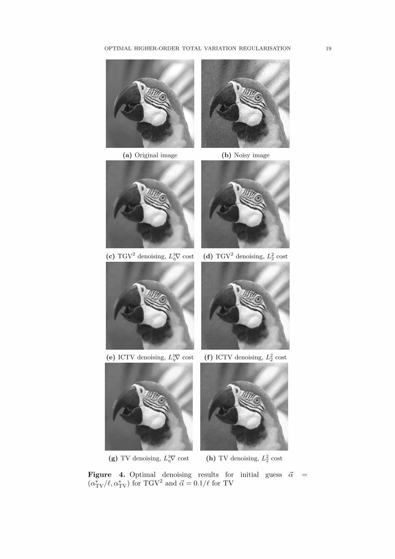
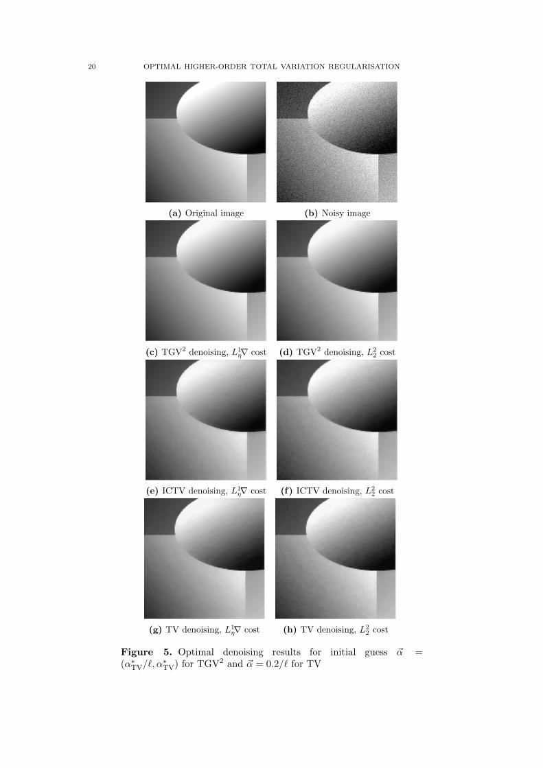
5.1. Gaussian denoising. We tested Algorithm 4.1 for TV and Algorithm 4.2 forTGV2 Gaussian denoising parameter learning on various images. Here we report theresults for two images, the parrot image in Figure 4a, and the geometric image inFigure 5. We applied synthetic noise to the original images, such that the PSNR ofthe parrot image is 24.7, and the PSNR of the geometric image is 24.8.
In order to learn the regularisation parameter α for TV, we picked initial α0 =0.1/`. For TGV2 initialisation by TV was used as in Algorithm 4.1. We chose theother parameters of Algorithm 4.1 as c = 1e−4, ρ = 1e−5, θ = 1e−8, and Θ = 10.For the SSN denoising method the parameters γ = 100 and µ = 1e−10 were chosen.
We have included results for both the L2-squared cost functional L22 and the Hu-
berised total variation cost functional L1η∇. The learning results are reported in
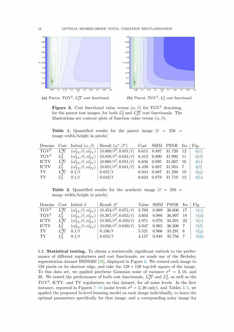
Table 1 for the parrot images, and Table 2 for the geometric image. The denoisingresults with the discovered parameters can be found in the aforementioned Figure 4and Figure 5. We report the resulting optimal parameter values, the cost functionalvalue, PSNR, SSIM [37], as well as the number of iterations taken by the outer BFGSmethod.
Our first observation is that all approaches successfully learn a denoising parameterthat gives a good-quality denoised image. Secondly, we observe that the gradient costfunctional L1
η∇ performs visually and in terms of SSIM significantly better for TGV2
parameter learning than the cost functional L22. In terms of PSNR the roles are
reversed, as should be, since the L22 is equivalent to PSNR. This again confirms that
PSNR is a poor quality measure for images. For TV there is no significant differencebetween different cost functionals in terms of visual quality, although the PSNR andSSIM differ.
We also observe that the optimal TGV2 parameters (α∗, β∗) generally satisfyβ∗/α∗ ∈ (0.75, 1.5)/`. This confirms the earlier observed heuristic that if ` ≈ 128, 256then β ∈ (1, 1.5)α tends to be a good choice. As we can observe from Figure 4 andFigure 5, this optimal TGV2 parameter choice also avoids the stair-casing effect thatcan be observed with TV in the results.
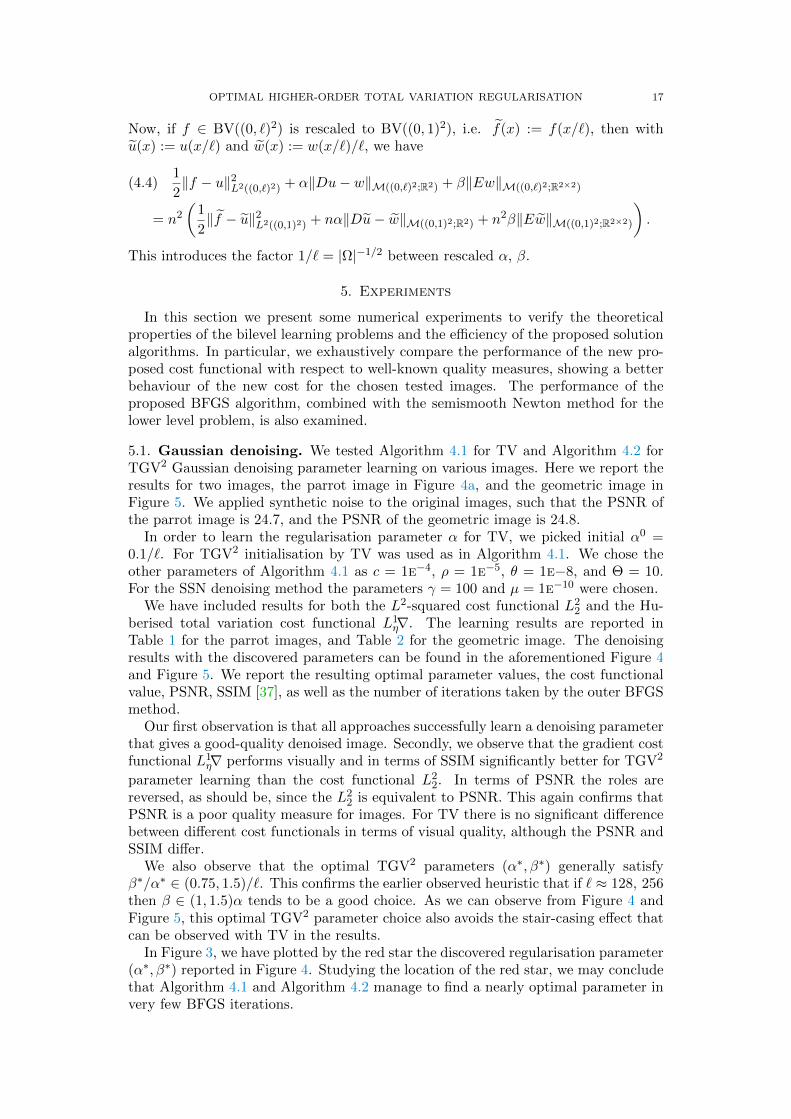
In Figure 3, we have plotted by the red star the discovered regularisation parameter(α∗, β∗) reported in Figure 4. Studying the location of the red star, we may concludethat Algorithm 4.1 and Algorithm 4.2 manage to find a nearly optimal parameter invery few BFGS iterations.
18 OPTIMAL HIGHER-ORDER TOTAL VARIATION REGULARISATION
0.05 0.1 0.15 0.2 0.25 0.3 0.35 0.4 0.45 0.5
0.05
0.1
0.15
0.2
0.25
0.3
0.35
0.4
0.45
0.5
α
β
(a) Parrot, TGV2, L1η∇ cost functional
0.05 0.1 0.15 0.2 0.25 0.3 0.35 0.4 0.45 0.5
0.05
0.1
0.15
0.2
0.25
0.3
0.35
0.4
0.45
0.5
α
β
(b) Parrot, TGV2, L22 cost functional
Figure 3. Cost functional value versus (α, β) for TGV2 denoising,for the parrot test images, for both L2
2 and L1η∇ cost functionals. The
illustrations are contour plots of function value versus (α, β).
Table 1. Quantified results for the parrot image (` = 256 =image width/height in pixels)
Denoise Cost Initial (α, β) Result (α∗, β∗) Cost SSIM PSNR Its. Fig.
TGV2 L1η∇ (α∗TV/`, α
∗TV) (0.069/`2, 0.051/`) 6.615 0.897 31.720 12 4(c)
TGV2 L22 (α∗TV/`, α
∗TV) (0.058/`2, 0.041/`) 6.412 0.890 31.992 11 4(d)
ICTV L1η∇ (α∗TV/`, α
∗TV) (0.068/`2, 0.051/`) 6.656 0.895 31.667 16 4(e)
ICTV L22 (α∗TV/`, α
∗TV) (0.051/`2, 0.041/`) 6.439 0.887 31.954 7 4(f)
TV L1η∇ 0.1/` 0.057/` 6.944 0.887 31.298 10 4(g)
TV L22 0.1/` 0.042/` 6.623 0.879 31.710 12 4(h)
Table 2. Quantified results for the synthetic image (` = 256 =image width/height in pixels)
Denoise Cost Initial ~α Result ~α∗ Value SSIM PSNR Its. Fig.
TGV2 L1η∇ (α∗TV/`, α
∗TV) (0.453/`2, 0.071/`) 3.769 0.989 36.606 17 5(c)
TGV2 L22 (α∗TV/`, α
∗TV) (0.307/`2, 0.055/`) 3.603 0.986 36.997 19 5(d)
ICTV L1η∇ (α∗TV/`, α
∗TV) (0.505/`2, 0.103/`) 4.971 0.970 34.201 23 5(e)
ICTV L22 (α∗TV/`, α
∗TV) (0.056/`2, 0.049/`) 3.947 0.965 36.206 7 5(f)
TV L1η∇ 0.1/` 0.136/` 5.521 0.966 33.291 6 5(g)
TV L22 0.1/` 0.052/` 4.157 0.948 35.756 7 5(h)
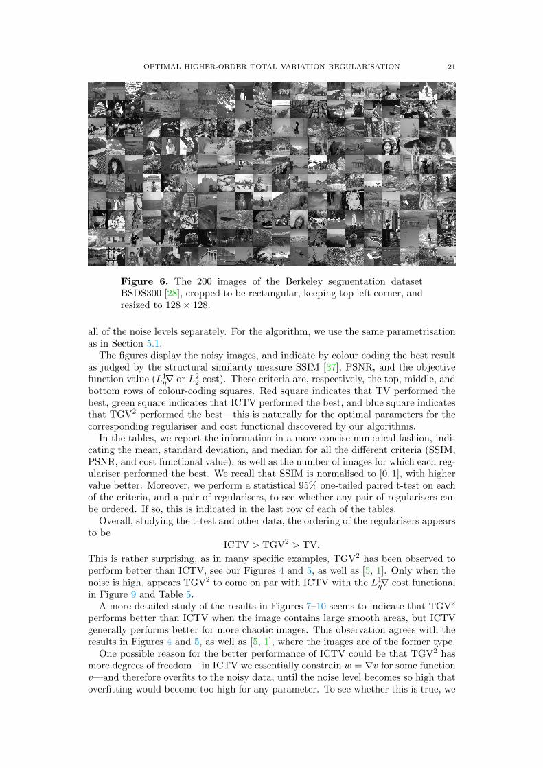
5.2. Statistical testing. To obtain a statistically significant outlook to the perfor-mance of different regularisers and cost functionals, we made use of the Berkeleysegmentation dataset BSDS300 [28], displayed in Figure 6. We resized each image to128 pixels on its shortest edge, and take the 128 × 128 top-left square of the image.To this data set, we applied pixelwise Gaussian noise of variance σ2 = 2, 10, and20. We tested the performance of both cost functionals, L1
η∇ and L22, as well as the
TGV2, ICTV, and TV regularisers on this dataset, for all noise levels. In the firstinstance, reported in Figures 7–10 (noise levels σ2 = 2, 20 only), and Tables 3–5, weapplied the proposed bi-level learning model on each image individually, to learn theoptimal parameters specifically for that image, and a correponding noisy image for
OPTIMAL HIGHER-ORDER TOTAL VARIATION REGULARISATION 19
(a) Original image (b) Noisy image
(c) TGV2 denoising, L1η∇ cost (d) TGV2 denoising, L2
2 cost
(e) ICTV denoising, L1η∇ cost (f) ICTV denoising, L2
2 cost
(g) TV denoising, L1η∇ cost (h) TV denoising, L2
2 cost
Figure 4. Optimal denoising results for initial guess ~α =(α∗TV/`, α
∗TV) for TGV2 and ~α = 0.1/` for TV
20 OPTIMAL HIGHER-ORDER TOTAL VARIATION REGULARISATION
(a) Original image (b) Noisy image
(c) TGV2 denoising, L1η∇ cost (d) TGV2 denoising, L2
2 cost
(e) ICTV denoising, L1η∇ cost (f) ICTV denoising, L2
2 cost
(g) TV denoising, L1η∇ cost (h) TV denoising, L2
2 cost
Figure 5. Optimal denoising results for initial guess ~α =(α∗TV/`, α
∗TV) for TGV2 and ~α = 0.2/` for TV
OPTIMAL HIGHER-ORDER TOTAL VARIATION REGULARISATION 21
Figure 6. The 200 images of the Berkeley segmentation datasetBSDS300 [28], cropped to be rectangular, keeping top left corner, andresized to 128× 128.
all of the noise levels separately. For the algorithm, we use the same parametrisationas in Section 5.1.
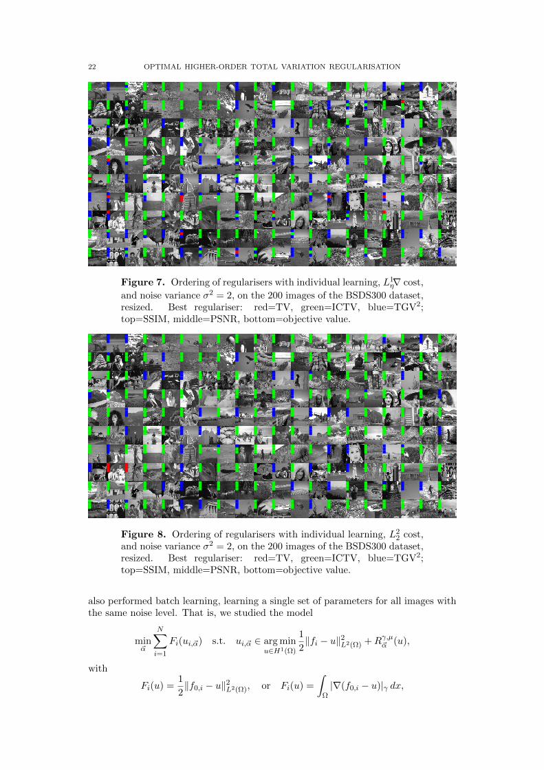
The figures display the noisy images, and indicate by colour coding the best resultas judged by the structural similarity measure SSIM [37], PSNR, and the objectivefunction value (L1
η∇ or L22 cost). These criteria are, respectively, the top, middle, and
bottom rows of colour-coding squares. Red square indicates that TV performed thebest, green square indicates that ICTV performed the best, and blue square indicatesthat TGV2 performed the best—this is naturally for the optimal parameters for thecorresponding regulariser and cost functional discovered by our algorithms.
In the tables, we report the information in a more concise numerical fashion, indi-cating the mean, standard deviation, and median for all the different criteria (SSIM,PSNR, and cost functional value), as well as the number of images for which each reg-ulariser performed the best. We recall that SSIM is normalised to [0, 1], with highervalue better. Moreover, we perform a statistical 95% one-tailed paired t-test on eachof the criteria, and a pair of regularisers, to see whether any pair of regularisers canbe ordered. If so, this is indicated in the last row of each of the tables.
Overall, studying the t-test and other data, the ordering of the regularisers appearsto be
ICTV > TGV2 > TV.
This is rather surprising, as in many specific examples, TGV2 has been observed toperform better than ICTV, see our Figures 4 and 5, as well as [5, 1]. Only when thenoise is high, appears TGV2 to come on par with ICTV with the L1
η∇ cost functionalin Figure 9 and Table 5.
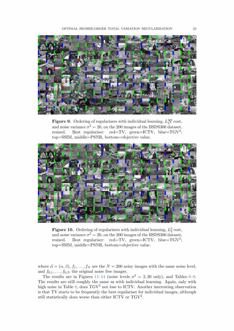
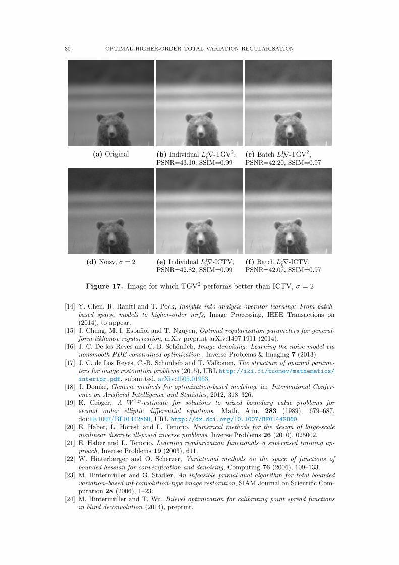
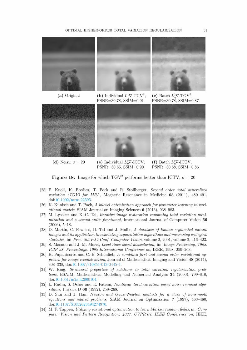
A more detailed study of the results in Figures 7–10 seems to indicate that TGV2
performs better than ICTV when the image contains large smooth areas, but ICTVgenerally performs better for more chaotic images. This observation agrees with theresults in Figures 4 and 5, as well as [5, 1], where the images are of the former type.
One possible reason for the better performance of ICTV could be that TGV2 hasmore degrees of freedom—in ICTV we essentially constrain w = ∇v for some functionv—and therefore overfits to the noisy data, until the noise level becomes so high thatoverfitting would become too high for any parameter. To see whether this is true, we
22 OPTIMAL HIGHER-ORDER TOTAL VARIATION REGULARISATION
Figure 7. Ordering of regularisers with individual learning, L1η∇ cost,
and noise variance σ2 = 2, on the 200 images of the BSDS300 dataset,resized. Best regulariser: red=TV, green=ICTV, blue=TGV2;top=SSIM, middle=PSNR, bottom=objective value.
Figure 8. Ordering of regularisers with individual learning, L22 cost,
and noise variance σ2 = 2, on the 200 images of the BSDS300 dataset,resized. Best regulariser: red=TV, green=ICTV, blue=TGV2;top=SSIM, middle=PSNR, bottom=objective value.
also performed batch learning, learning a single set of parameters for all images withthe same noise level. That is, we studied the model
min~α
N∑i=1
Fi(ui,~α) s.t. ui,~α ∈ arg minu∈H1(Ω)
1
2‖fi − u‖2L2(Ω) +Rγ,µ~α (u),
with
Fi(u) =1
2‖f0,i − u‖2L2(Ω), or Fi(u) =
∫Ω|∇(f0,i − u)|γ dx,
OPTIMAL HIGHER-ORDER TOTAL VARIATION REGULARISATION 23
Figure 9. Ordering of regularisers with individual learning, L1η∇ cost,
and noise variance σ2 = 20, on the 200 images of the BSDS300 dataset,resized. Best regulariser: red=TV, green=ICTV, blue=TGV2;top=SSIM, middle=PSNR, bottom=objective value.
Figure 10. Ordering of regularisers with individual learning, L22 cost,
and noise variance σ2 = 20, on the 200 images of the BSDS300 dataset,resized. Best regulariser: red=TV, green=ICTV, blue=TGV2;top=SSIM, middle=PSNR, bottom=objective value.
where ~α = (α, β), f1, . . . , fN are the N = 200 noisy images with the same noise level,and f0,1, . . . , f0,N the original noise free images.
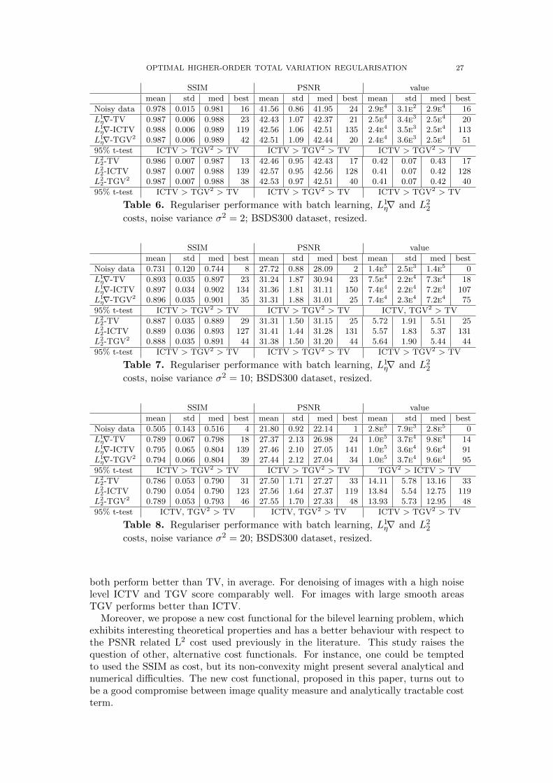
The results are in Figures 11–14 (noise levels σ2 = 2, 20 only), and Tables 6–8.The results are still roughly the same as with individual learning. Again, only withhigh noise in Table 8, does TGV2 not lose to ICTV. Another interesting observationis that TV starts to be frequently the best regulariser for individual images, althoughstill statistically does worse than either ICTV or TGV2.
24 OPTIMAL HIGHER-ORDER TOTAL VARIATION REGULARISATION
SSIM PSNR value
mean std med best mean std med best mean std med best
Noisy data 0.978 0.015 0.981 0 41.56 0.86 41.95 0 2.9e4 3.1e2 2.9e4 0
L1η∇-TV 0.988 0.005 0.989 1 42.57 1.10 42.46 5 2.4e4 3.7e3 2.5e4 1
L1η∇-ICTV 0.989 0.005 0.990 141 42.74 1.16 42.62 143 2.3e4 3.9e3 2.4e4 137
L1η∇-TGV2 0.989 0.005 0.989 58 42.70 1.17 42.55 52 2.4e4 4.0e3 2.5e4 62
95% t-test ICTV > TGV2 > TV ICTV > TGV2 > TV ICTV > TGV2 > TV
L22-TV 0.988 0.005 0.988 2 42.64 1.14 42.50 2 0.41 0.08 0.43 2
L22-ICTV 0.988 0.005 0.989 142 42.79 1.18 42.64 148 0.39 0.08 0.41 148
L22-TGV2 0.988 0.005 0.989 56 42.76 1.19 42.58 50 0.40 0.08 0.42 50
95% t-test ICTV > TGV2 > TV ICTV > TGV2 > TV ICTV > TGV2 > TV
Table 3. Regulariser performance with individual learning, L22 and
L1η∇ costs and noise variance σ2 = 2; BSDS300 dataset, resized.
SSIM PSNR value
mean std med best mean std med best mean std med best
Noisy data 0.731 0.120 0.744 0 27.72 0.88 28.09 0 1.4e5 2.5e3 1.4e5 0
L1η∇-TV 0.898 0.036 0.900 4 31.28 1.63 30.97 8 7.3e4 2.2e4 7.3e4 1
L1η∇-ICTV 0.906 0.034 0.909 139 31.54 1.68 31.21 142 7.1e4 2.2e4 7.1e4 121
L1η∇-TGV2 0.905 0.035 0.907 57 31.47 1.72 31.10 50 7.1e4 2.2e4 7.1e4 78
95% t-test ICTV > TGV2 > TV ICTV > TGV2 > TV ICTV > TGV2 > TV
L22-TV 0.897 0.033 0.898 9 31.54 1.76 31.15 2 5.52 1.89 5.51 2
L22-ICTV 0.903 0.032 0.903 131 31.72 1.76 31.33 148 5.30 1.81 5.35 148
L22-TGV2 0.902 0.033 0.903 60 31.67 1.80 31.28 50 5.38 1.87 5.39 50
95% t-test ICTV > TGV2 > TV ICTV > TGV2 > TV ICTV > TGV2 > TV
Table 4. Regulariser performance with individual learning, L22 and
L1η∇ costs and noise variance σ2 = 10; BSDS300 dataset, resized.
SSIM PSNR value
mean std med best mean std med best mean std med best
Noisy data 0.505 0.143 0.516 0 21.80 0.92 22.14 0 2.8e5 7.9e3 2.8e5 0
L1η∇-TV 0.795 0.063 0.799 7 27.27 1.64 27.02 11 1.0e5 3.5e4 9.7e4 1
L1η∇-ICTV 0.810 0.061 0.814 120 27.52 1.66 27.24 125 9.7e4 3.4e4 9.6e4 79
L1η∇-TGV2 0.808 0.062 0.814 73 27.50 1.74 27.15 64 9.8e4 3.5e4 9.5e4 120
95% t-test ICTV > TGV2 > TV ICTV, TGV2 > TV ICTV, TGV2 > TV
L22-TV 0.802 0.056 0.804 8 27.70 1.93 27.28 0 13.65 5.53 13.14 0
L22-ICTV 0.811 0.056 0.816 126 27.86 1.91 27.45 138 13.14 5.22 12.62 138
L22-TGV2 0.810 0.057 0.814 66 27.83 1.94 27.41 62 13.28 5.38 12.77 62
95% t-test ICTV > TGV2 > TV ICTV > TGV2 > TV ICTV > TGV2 > TV
Table 5. Regulariser performance with individual learning, L22 and
L1η∇ costs and noise variance σ2 = 20; BSDS300 dataset, resized.
For the first image of the data set, ICTV does in all of the Figures 7–14 betterthan TGV2, while for the second image, the situation is reversed. We have highlightedthese two images for the L1
η∇ cost in Figures 15–18, for both noise levels σ = 2 andσ = 20. In the case where ICTV does better, hardly any difference can be observedby the eye, while for second image TGV2 clearly has less stair-casing in the smoothareas of the image, especially with the noise level σ = 20.
Based on this study, it therefore seems that ICTV is the most reliable regulariser ofthe ones tested, when the type of image being processed is unknown, and low SSIM,PSNR or L1
η∇ cost functional value is desired. But as can be observed for individualimages, it can within large smooth areas exhibit artefacts that are avoided by the useof TGV2.

OPTIMAL HIGHER-ORDER TOTAL VARIATION REGULARISATION 25
Figure 11. Ordering of regularisers with batch learning, L1η∇ cost,
and noise variance σ2 = 2, on the 200 images of the BSDS300 dataset,resized. Best regulariser: red=TV, green=ICTV, blue=TGV2;top=SSIM, middle=PSNR, bottom=objective value.
Figure 12. Ordering of regularisers with batch learning, L22 cost, and
noise variance σ2 = 2, on the 200 images of the BSDS300 dataset,resized. Best regulariser: red=TV, green=ICTV, blue=TGV2;top=SSIM, middle=PSNR, bottom=objective value.
5.3. The choice of cost functional. The L22 cost functional naturally obtains bet-
ter PSNR than L1η∇, as the two former are equivalent. Comparing the results for
the two cost funtionals in Tables 3–5, we may however observe that for low noiselevels σ2 = 2, 10, and generally for batch learning, L1
η∇ attains better (higher) SSIM.Since SSIM better captures [37] the visual quality of images than PSNR, this recom-mends the use of our novel total variation cost functional L1
η∇. Of course, one mightattempt to optimise the SSIM. This is however a non-convex functional, which willpose additional numerical challenges avoided by the convex total variation cost.
26 OPTIMAL HIGHER-ORDER TOTAL VARIATION REGULARISATION
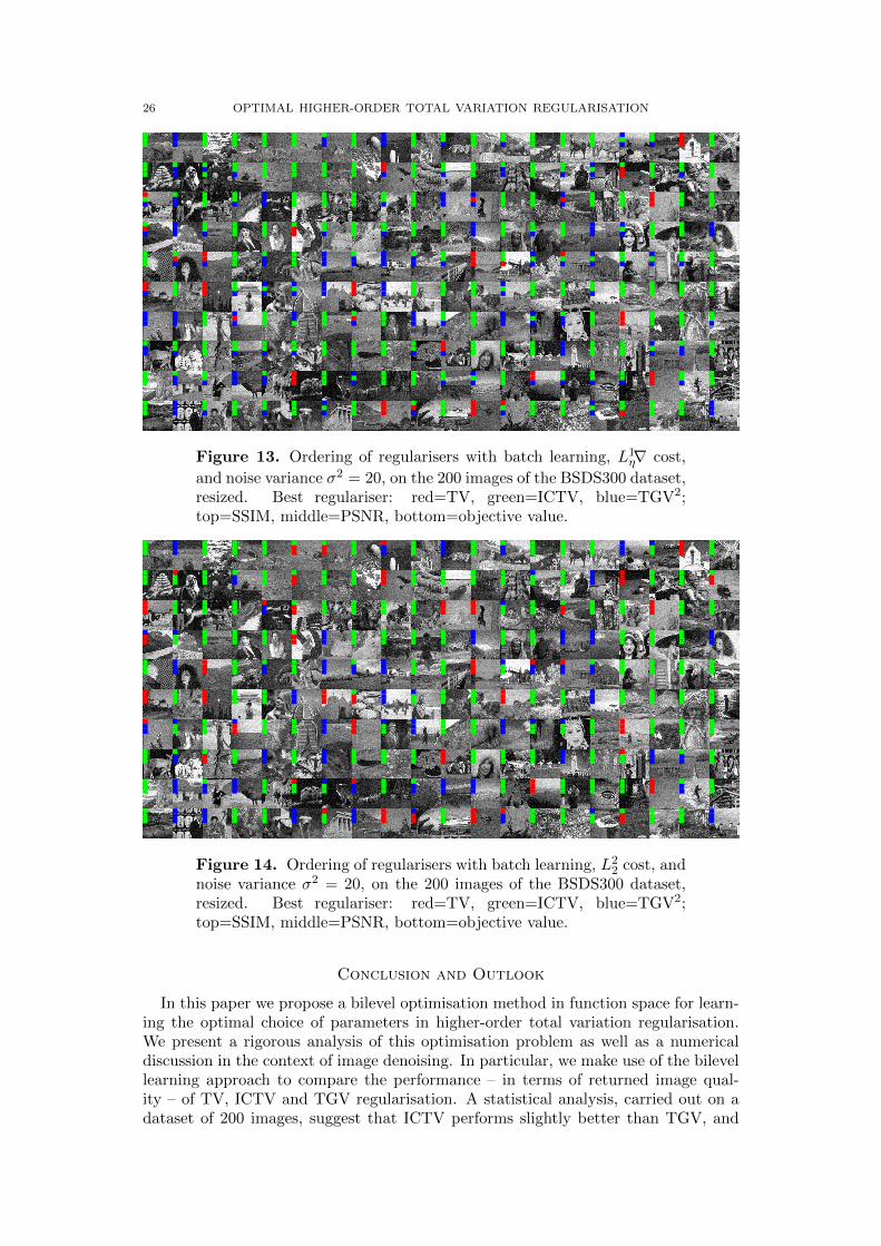
Figure 13. Ordering of regularisers with batch learning, L1η∇ cost,
and noise variance σ2 = 20, on the 200 images of the BSDS300 dataset,resized. Best regulariser: red=TV, green=ICTV, blue=TGV2;top=SSIM, middle=PSNR, bottom=objective value.
Figure 14. Ordering of regularisers with batch learning, L22 cost, and
noise variance σ2 = 20, on the 200 images of the BSDS300 dataset,resized. Best regulariser: red=TV, green=ICTV, blue=TGV2;top=SSIM, middle=PSNR, bottom=objective value.
Conclusion and Outlook
In this paper we propose a bilevel optimisation method in function space for learn-ing the optimal choice of parameters in higher-order total variation regularisation.We present a rigorous analysis of this optimisation problem as well as a numericaldiscussion in the context of image denoising. In particular, we make use of the bilevellearning approach to compare the performance – in terms of returned image qual-ity – of TV, ICTV and TGV regularisation. A statistical analysis, carried out on adataset of 200 images, suggest that ICTV performs slightly better than TGV, and
OPTIMAL HIGHER-ORDER TOTAL VARIATION REGULARISATION 27
SSIM PSNR value
mean std med best mean std med best mean std med best
Noisy data 0.978 0.015 0.981 16 41.56 0.86 41.95 24 2.9e4 3.1e2 2.9e4 16
L1η∇-TV 0.987 0.006 0.988 23 42.43 1.07 42.37 21 2.5e4 3.4e3 2.5e4 20
L1η∇-ICTV 0.988 0.006 0.989 119 42.56 1.06 42.51 135 2.4e4 3.5e3 2.5e4 113
L1η∇-TGV2 0.987 0.006 0.989 42 42.51 1.09 42.44 20 2.4e4 3.6e3 2.5e4 51
95% t-test ICTV > TGV2 > TV ICTV > TGV2 > TV ICTV > TGV2 > TV
L22-TV 0.986 0.007 0.987 13 42.46 0.95 42.43 17 0.42 0.07 0.43 17
L22-ICTV 0.987 0.007 0.988 139 42.57 0.95 42.56 128 0.41 0.07 0.42 128
L22-TGV2 0.987 0.007 0.988 38 42.53 0.97 42.51 40 0.41 0.07 0.42 40
95% t-test ICTV > TGV2 > TV ICTV > TGV2 > TV ICTV > TGV2 > TV
Table 6. Regulariser performance with batch learning, L1η∇ and L2
2
costs, noise variance σ2 = 2; BSDS300 dataset, resized.
SSIM PSNR value
mean std med best mean std med best mean std med best
Noisy data 0.731 0.120 0.744 8 27.72 0.88 28.09 2 1.4e5 2.5e3 1.4e5 0
L1η∇-TV 0.893 0.035 0.897 23 31.24 1.87 30.94 23 7.5e4 2.2e4 7.3e4 18
L1η∇-ICTV 0.897 0.034 0.902 134 31.36 1.81 31.11 150 7.4e4 2.2e4 7.2e4 107
L1η∇-TGV2 0.896 0.035 0.901 35 31.31 1.88 31.01 25 7.4e4 2.3e4 7.2e4 75
95% t-test ICTV > TGV2 > TV ICTV > TGV2 > TV ICTV, TGV2 > TV
L22-TV 0.887 0.035 0.889 29 31.31 1.50 31.15 25 5.72 1.91 5.51 25
L22-ICTV 0.889 0.036 0.893 127 31.41 1.44 31.28 131 5.57 1.83 5.37 131
L22-TGV2 0.888 0.035 0.891 44 31.38 1.50 31.20 44 5.64 1.90 5.44 44
95% t-test ICTV > TGV2 > TV ICTV > TGV2 > TV ICTV > TGV2 > TV
Table 7. Regulariser performance with batch learning, L1η∇ and L2
2
costs, noise variance σ2 = 10; BSDS300 dataset, resized.
SSIM PSNR value
mean std med best mean std med best mean std med best
Noisy data 0.505 0.143 0.516 4 21.80 0.92 22.14 1 2.8e5 7.9e3 2.8e5 0
L1η∇-TV 0.789 0.067 0.798 18 27.37 2.13 26.98 24 1.0e5 3.7e4 9.8e4 14
L1η∇-ICTV 0.795 0.065 0.804 139 27.46 2.10 27.05 141 1.0e5 3.6e4 9.6e4 91
L1η∇-TGV2 0.794 0.066 0.804 39 27.44 2.12 27.04 34 1.0e5 3.7e4 9.6e4 95
95% t-test ICTV > TGV2 > TV ICTV > TGV2 > TV TGV2 > ICTV > TV
L22-TV 0.786 0.053 0.790 31 27.50 1.71 27.27 33 14.11 5.78 13.16 33
L22-ICTV 0.790 0.054 0.790 123 27.56 1.64 27.37 119 13.84 5.54 12.75 119
L22-TGV2 0.789 0.053 0.793 46 27.55 1.70 27.33 48 13.93 5.73 12.95 48
95% t-test ICTV, TGV2 > TV ICTV, TGV2 > TV ICTV > TGV2 > TV
Table 8. Regulariser performance with batch learning, L1η∇ and L2
2
costs, noise variance σ2 = 20; BSDS300 dataset, resized.
both perform better than TV, in average. For denoising of images with a high noiselevel ICTV and TGV score comparably well. For images with large smooth areasTGV performs better than ICTV.
Moreover, we propose a new cost functional for the bilevel learning problem, whichexhibits interesting theoretical properties and has a better behaviour with respect tothe PSNR related L2 cost used previously in the literature. This study raises thequestion of other, alternative cost functionals. For instance, one could be temptedto used the SSIM as cost, but its non-convexity might present several analytical andnumerical difficulties. The new cost functional, proposed in this paper, turns out tobe a good compromise between image quality measure and analytically tractable costterm.
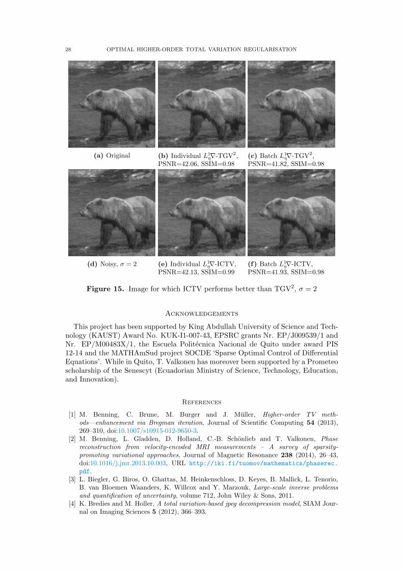
28 OPTIMAL HIGHER-ORDER TOTAL VARIATION REGULARISATION
(a) Original (b) Individual L1η∇-TGV2,
PSNR=42.06, SSIM=0.98(c) Batch L1
η∇-TGV2,PSNR=41.82, SSIM=0.98
(d) Noisy, σ = 2 (e) Individual L1η∇-ICTV,
PSNR=42.13, SSIM=0.99(f) Batch L1
η∇-ICTV,PSNR=41.93, SSIM=0.98
Figure 15. Image for which ICTV performs better than TGV2, σ = 2
Acknowledgements
This project has been supported by King Abdullah University of Science and Tech-nology (KAUST) Award No. KUK-I1-007-43, EPSRC grants Nr. EP/J009539/1 andNr. EP/M00483X/1, the Escuela Politecnica Nacional de Quito under award PIS12-14 and the MATHAmSud project SOCDE ‘Sparse Optimal Control of DifferentialEquations’. While in Quito, T. Valkonen has moreover been supported by a Prometeoscholarship of the Senescyt (Ecuadorian Ministry of Science, Technology, Education,and Innovation).
References
[1] M. Benning, C. Brune, M. Burger and J. Muller, Higher-order TV meth-ods—enhancement via Bregman iteration, Journal of Scientific Computing 54 (2013),269–310, doi:10.1007/s10915-012-9650-3.
[2] M. Benning, L. Gladden, D. Holland, C.-B. Schonlieb and T. Valkonen, Phasereconstruction from velocity-encoded MRI measurements – A survey of sparsity-promoting variational approaches, Journal of Magnetic Resonance 238 (2014), 26–43,doi:10.1016/j.jmr.2013.10.003, URL http://iki.fi/tuomov/mathematics/phaserec.
pdf.[3] L. Biegler, G. Biros, O. Ghattas, M. Heinkenschloss, D. Keyes, B. Mallick, L. Tenorio,
B. van Bloemen Waanders, K. Willcox and Y. Marzouk, Large-scale inverse problemsand quantification of uncertainty, volume 712, John Wiley & Sons, 2011.
[4] K. Bredies and M. Holler, A total variation-based jpeg decompression model, SIAM Jour-nal on Imaging Sciences 5 (2012), 366–393.
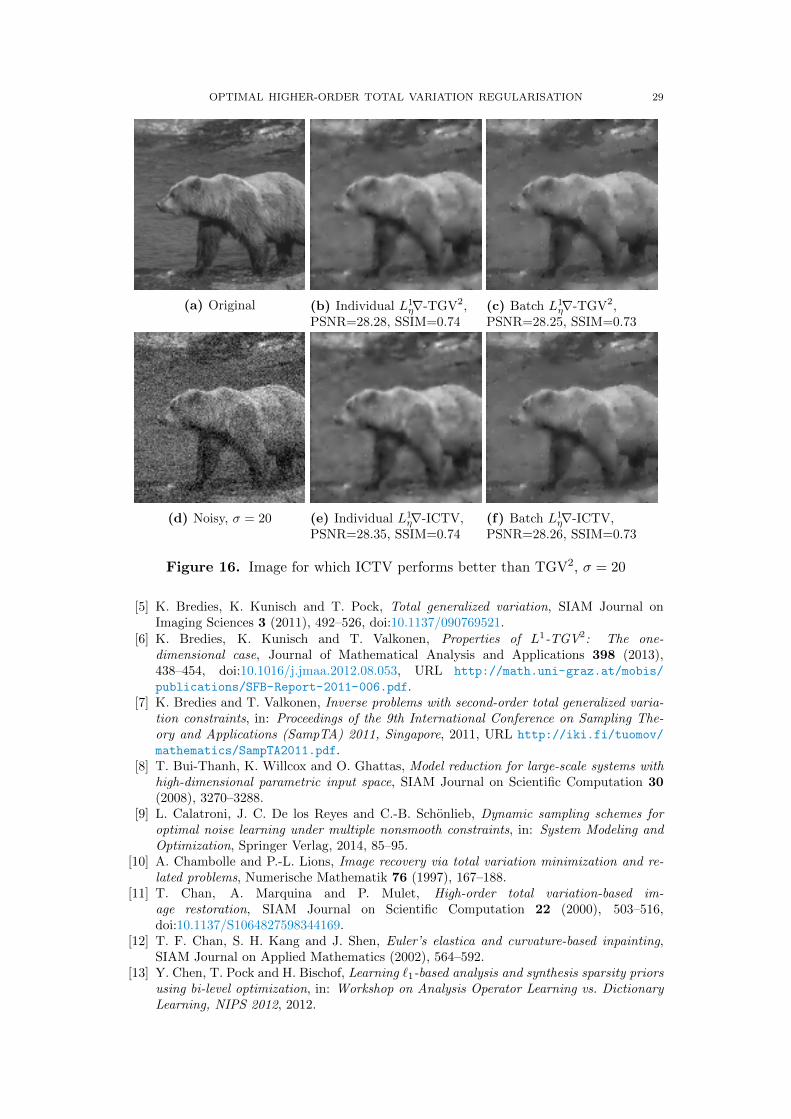
OPTIMAL HIGHER-ORDER TOTAL VARIATION REGULARISATION 29
(a) Original (b) Individual L1η∇-TGV2,
PSNR=28.28, SSIM=0.74(c) Batch L1
η∇-TGV2,PSNR=28.25, SSIM=0.73
(d) Noisy, σ = 20 (e) Individual L1η∇-ICTV,
PSNR=28.35, SSIM=0.74(f) Batch L1
η∇-ICTV,PSNR=28.26, SSIM=0.73
Figure 16. Image for which ICTV performs better than TGV2, σ = 20
[5] K. Bredies, K. Kunisch and T. Pock, Total generalized variation, SIAM Journal onImaging Sciences 3 (2011), 492–526, doi:10.1137/090769521.
[6] K. Bredies, K. Kunisch and T. Valkonen, Properties of L1-TGV2: The one-dimensional case, Journal of Mathematical Analysis and Applications 398 (2013),438–454, doi:10.1016/j.jmaa.2012.08.053, URL http://math.uni-graz.at/mobis/
publications/SFB-Report-2011-006.pdf.[7] K. Bredies and T. Valkonen, Inverse problems with second-order total generalized varia-
tion constraints, in: Proceedings of the 9th International Conference on Sampling The-ory and Applications (SampTA) 2011, Singapore, 2011, URL http://iki.fi/tuomov/
mathematics/SampTA2011.pdf.[8] T. Bui-Thanh, K. Willcox and O. Ghattas, Model reduction for large-scale systems with
high-dimensional parametric input space, SIAM Journal on Scientific Computation 30(2008), 3270–3288.
[9] L. Calatroni, J. C. De los Reyes and C.-B. Schonlieb, Dynamic sampling schemes foroptimal noise learning under multiple nonsmooth constraints, in: System Modeling andOptimization, Springer Verlag, 2014, 85–95.
[10] A. Chambolle and P.-L. Lions, Image recovery via total variation minimization and re-lated problems, Numerische Mathematik 76 (1997), 167–188.
[11] T. Chan, A. Marquina and P. Mulet, High-order total variation-based im-age restoration, SIAM Journal on Scientific Computation 22 (2000), 503–516,doi:10.1137/S1064827598344169.
[12] T. F. Chan, S. H. Kang and J. Shen, Euler’s elastica and curvature-based inpainting,SIAM Journal on Applied Mathematics (2002), 564–592.
[13] Y. Chen, T. Pock and H. Bischof, Learning `1-based analysis and synthesis sparsity priorsusing bi-level optimization, in: Workshop on Analysis Operator Learning vs. DictionaryLearning, NIPS 2012, 2012.
30 OPTIMAL HIGHER-ORDER TOTAL VARIATION REGULARISATION
(a) Original (b) Individual L1η∇-TGV2,
PSNR=43.10, SSIM=0.99(c) Batch L1
η∇-TGV2,PSNR=42.20, SSIM=0.97
(d) Noisy, σ = 2 (e) Individual L1η∇-ICTV,
PSNR=42.82, SSIM=0.99(f) Batch L1
η∇-ICTV,PSNR=42.07, SSIM=0.97
Figure 17. Image for which TGV2 performs better than ICTV, σ = 2
[14] Y. Chen, R. Ranftl and T. Pock, Insights into analysis operator learning: From patch-based sparse models to higher-order mrfs, Image Processing, IEEE Transactions on(2014), to appear.
[15] J. Chung, M. I. Espanol and T. Nguyen, Optimal regularization parameters for general-form tikhonov regularization, arXiv preprint arXiv:1407.1911 (2014).
[16] J. C. De los Reyes and C.-B. Schonlieb, Image denoising: Learning the noise model vianonsmooth PDE-constrained optimization., Inverse Problems & Imaging 7 (2013).
[17] J. C. de Los Reyes, C.-B. Schonlieb and T. Valkonen, The structure of optimal parame-ters for image restoration problems (2015), URL http://iki.fi/tuomov/mathematics/
interior.pdf, submitted, arXiv:1505.01953.[18] J. Domke, Generic methods for optimization-based modeling, in: International Confer-
ence on Artificial Intelligence and Statistics, 2012, 318–326.[19] K. Groger, A W 1,p-estimate for solutions to mixed boundary value problems for
second order elliptic differential equations, Math. Ann. 283 (1989), 679–687,doi:10.1007/BF01442860, URL http://dx.doi.org/10.1007/BF01442860.
[20] E. Haber, L. Horesh and L. Tenorio, Numerical methods for the design of large-scalenonlinear discrete ill-posed inverse problems, Inverse Problems 26 (2010), 025002.
[21] E. Haber and L. Tenorio, Learning regularization functionals–a supervised training ap-proach, Inverse Problems 19 (2003), 611.
[22] W. Hinterberger and O. Scherzer, Variational methods on the space of functions ofbounded hessian for convexification and denoising, Computing 76 (2006), 109–133.
[23] M. Hintermuller and G. Stadler, An infeasible primal-dual algorithm for total boundedvariation–based inf-convolution-type image restoration, SIAM Journal on Scientific Com-putation 28 (2006), 1–23.
[24] M. Hintermuller and T. Wu, Bilevel optimization for calibrating point spread functionsin blind deconvolution (2014), preprint.
OPTIMAL HIGHER-ORDER TOTAL VARIATION REGULARISATION 31
(a) Original (b) Individual L1η∇-TGV2,
PSNR=30.78, SSIM=0.91(c) Batch L1
η∇-TGV2,PSNR=30.78, SSIM=0.87
(d) Noisy, σ = 20 (e) Individual L1η∇-ICTV,
PSNR=30.55, SSIM=0.90(f) Batch L1
η∇-ICTV,PSNR=30.68, SSIM=0.86
Figure 18. Image for which TGV2 performs better than ICTV, σ = 20
[25] F. Knoll, K. Bredies, T. Pock and R. Stollberger, Second order total generalizedvariation (TGV) for MRI., Magnetic Resonance in Medicine 65 (2011), 480–491,doi:10.1002/mrm.22595.
[26] K. Kunisch and T. Pock, A bilevel optimization approach for parameter learning in vari-ational models, SIAM Journal on Imaging Sciences 6 (2013), 938–983.
[27] M. Lysaker and X.-C. Tai, Iterative image restoration combining total variation mini-mization and a second-order functional, International Journal of Computer Vision 66(2006), 5–18.
[28] D. Martin, C. Fowlkes, D. Tal and J. Malik, A database of human segmented naturalimages and its application to evaluating segmentation algorithms and measuring ecologicalstatistics, in: Proc. 8th Int’l Conf. Computer Vision, volume 2, 2001, volume 2, 416–423.
[29] S. Masnou and J.-M. Morel, Level lines based disocclusion, in: Image Processing, 1998.ICIP 98. Proceedings. 1998 International Conference on, IEEE, 1998, 259–263.
[30] K. Papafitsoros and C.-B. Schonlieb, A combined first and second order variational ap-proach for image reconstruction, Journal of Mathematical Imaging and Vision 48 (2014),308–338, doi:10.1007/s10851-013-0445-4.
[31] W. Ring, Structural properties of solutions to total variation regularization prob-lems, ESAIM: Mathematical Modelling and Numerical Analysis 34 (2000), 799–810,doi:10.1051/m2an:2000104.
[32] L. Rudin, S. Osher and E. Fatemi, Nonlinear total variation based noise removal algo-rithms, Physica D 60 (1992), 259–268.
[33] D. Sun and J. Han, Newton and Quasi-Newton methods for a class of nonsmoothequations and related problems, SIAM Journal on Optimization 7 (1997), 463–480,doi:10.1137/S1052623494274970.
[34] M. F. Tappen, Utilizing variational optimization to learn Markov random fields, in: Com-puter Vision and Pattern Recognition, 2007. CVPR’07. IEEE Conference on, IEEE,
32 OPTIMAL HIGHER-ORDER TOTAL VARIATION REGULARISATION
2007, 1–8.[35] T. Valkonen, K. Bredies and F. Knoll, Total generalised variation in diffusion tensor
imaging, SIAM Journal on Imaging Sciences 6 (2013), 487–525, doi:10.1137/120867172,URL http://iki.fi/tuomov/mathematics/dtireg.pdf.
[36] F. Viola, A. Fitzgibbon and R. Cipolla, A unifying resolution-independent formulationfor early vision, in: Computer Vision and Pattern Recognition (CVPR), 2012 IEEEConference on, IEEE, 2012, 494–501.
[37] Z. Wang, A. C. Bovik, H. R. Sheikh and E. P. Simoncelli, Image quality assessment:From error visibility to structural similarity, IEEE Transactions on Image Processing 13(2004), 600–612, doi:10.1109/TIP.2003.819861.
[38] J. Zowe and S. Kurcyusz, Regularity and stability for the mathematical programmingproblem in Banach spaces, Appl. Math. Optim. 5 (1979), 49–62.


![[S. Dempe] Foundations of Bilevel Programming (Non(Bookos.org)](https://static.fdocuments.net/doc/165x107/55cf9dde550346d033af9c7c/s-dempe-foundations-of-bilevel-programming-nonbookosorg-56b96b35f272c.jpg)