big.LITTLE HEVC - Energy Efficient Video Codec for Mobile ... · big.LITTLE HEVC - Energy...
94
big.LITTLE HEVC - Energy Efficient Video Codec for Mobile Platforms Cl´ audio Jos ´ e Matias Val´ erio Thesis to obtain the Master of Science Degree in Electrical and Computer Engineering Supervisors: Dr. Nuno Filipe Valentim Roma Dr. Pedro Filipe Zeferino Tom´ as Examination Committee Chairperson: Dr. Nuno Cavaco Gomes Horta Supervisor: Dr. Nuno Filipe Valentim Roma Member of the Committee: Dr. Rui Fuentecilla Maia Ferreira Neves May 2016
Transcript of big.LITTLE HEVC - Energy Efficient Video Codec for Mobile ... · big.LITTLE HEVC - Energy...
big.LITTLE HEVC - Energy Efficient Video Codec forMobile Platforms
Claudio Jose Matias Valerio
Thesis to obtain the Master of Science Degree inElectrical and Computer Engineering
Supervisors: Dr. Nuno Filipe Valentim RomaDr. Pedro Filipe Zeferino Tomas
Examination CommitteeChairperson: Dr. Nuno Cavaco Gomes HortaSupervisor: Dr. Nuno Filipe Valentim Roma
Member of the Committee: Dr. Rui Fuentecilla Maia Ferreira Neves
May 2016


Acknowledgments
I would like to thank my supervisors, Doutor Nuno Roma and Doutor Pedro Tomas, for their
guidance and advice throughout the development of this thesis as well as for all the revisions
of the final work. I would also like to thank all the support I got from family and friends over
this period. Finally, I would like to thank IST and INESC-ID for all the resources made available,
without which this thesis could not have been completed.

Abstract
To satisfy the growing demands for computation in mobile application domains, while still com-
plying with strict energy consumptions, several heterogeneous processor architectures have been
presented. One particular example is the ARM big.LITTLE, which aggregates two different clus-
ters of CPUs: one offering a slower and low-power profile, while the other is composed of more
powerful CPUs, characterized by a greater energy consumption. In accordance, to satisfy the
commitment of strict energy constraints in mobile video applications based on the HEVC stan-
dard, this thesis proposes the integration of a dedicated controller in the encoder loop, particu-
larly optimized for implementations based on the big.LITTLE processor. The developed controller
performs an energy-aware real-time parameterization of the video encoder, in order to simultane-
ously satisfy several target constraints concerning the encoding performance, energy efficiency,
bit-rate and video quality. To attain such objective, it offers the system designer a set of optimiza-
tion profiles, which define the commitment priority of the considered optimization metrics when
unable to satisfy all the constraints. The conducted experimental evaluation demonstrated the
ability of the developed controller to successfully follow the defined constraints and profiles, at the
cost of an insignificant computational overhead.
Keywords
ARM big.LITTLE, HEVC video encoder, energy-aware real-time parameterization, energy ef-
ficiency
iii


Resumo
Para satisfazer a crescente procura de processamento no domınio das aplicacoes moveis,
que cumpra restricoes energeticas rigorosas, foram apresentadas varias arquitecturas de proces-
sadores heterogeneas. Um exemplo em particular e o ARM big.LITTLE, que agrega dois clusters
de CPUs: um oferecendo um perfil mais lento e maior eficiencia energetica, enquanto o outro
e composto por CPU mais poderosos, caracterizados por um maior consumo energetico. De
acordo, para satisfazer o compromisso de limitacoes de energia rigorosas em aplicacoes de vıdeo
moveis baseadas no HEVC standard, esta tese propoe a integracao de um controlador dedicado
na malha de codificacao, particularmente otimizado para implementacoes baseadas no proces-
sador big.LITTLE. O controlador desenvolvido concretiza, em tempo real, uma parametrizacao do
codificador de vıdeo energeticamente consciente, de modo a satisfazer simultaneamente varias
restricoes ao nıvel do desempenho de codificacao, eficiencia energetica, bit-rate e qualidade de
vıdeo. Para alcancar este objectivo, e oferecido ao designer do sistema um conjunto de perfis de
otimizacao, que definem um compromisso entre as diversas metricas a otimizar quando nao se
consegue cumprir todas as restricoes. A avaliacao experimental realizada demonstra a capaci-
dade do controlador desenvolvido cumprir as restricoes e perfis definidos com sucesso, a custa
de um overhead computacional insignificante.
Palavras Chave
ARM big.LITTLE, codificador de vıdeo HEVC, parametrizacao do codificador de vıdeo ener-
geticamente consciente, eficiencia energetica
v


Contents
1 Introduction 2
1.1 Motivation . . . . . . . . . . . . . . . . . . . . . . . . . . . . . . . . . . . . . . . . . 3
1.2 Objectives . . . . . . . . . . . . . . . . . . . . . . . . . . . . . . . . . . . . . . . . . 3
1.3 Main contributions . . . . . . . . . . . . . . . . . . . . . . . . . . . . . . . . . . . . 4
1.4 Dissertation outline . . . . . . . . . . . . . . . . . . . . . . . . . . . . . . . . . . . . 4
2 High Efficiency Video Coding 5
2.1 HEVC standard . . . . . . . . . . . . . . . . . . . . . . . . . . . . . . . . . . . . . . 6
2.1.1 Sampled Representation of Pictures . . . . . . . . . . . . . . . . . . . . . . 7
2.1.2 Subdivision of pictures . . . . . . . . . . . . . . . . . . . . . . . . . . . . . . 7
2.1.3 Intra Prediction . . . . . . . . . . . . . . . . . . . . . . . . . . . . . . . . . . 8
2.1.4 Inter Prediction . . . . . . . . . . . . . . . . . . . . . . . . . . . . . . . . . . 8
2.1.5 Transform, Scaling, and Quantization . . . . . . . . . . . . . . . . . . . . . 10
2.1.6 Entropy coding . . . . . . . . . . . . . . . . . . . . . . . . . . . . . . . . . . 10
2.1.7 In-Loop Filters . . . . . . . . . . . . . . . . . . . . . . . . . . . . . . . . . . 11
2.1.8 Profiles . . . . . . . . . . . . . . . . . . . . . . . . . . . . . . . . . . . . . . 11
2.2 Parallelization approaches to video coding . . . . . . . . . . . . . . . . . . . . . . . 11
2.2.1 Parallel Processing Platforms . . . . . . . . . . . . . . . . . . . . . . . . . . 12
2.2.2 Parallel implementations of video coding . . . . . . . . . . . . . . . . . . . . 12
2.2.2.A GOP-level Parallelism . . . . . . . . . . . . . . . . . . . . . . . . . 13
2.2.2.B Frame-level Parallelism . . . . . . . . . . . . . . . . . . . . . . . . 13
2.2.2.C Slice-level Parallelism . . . . . . . . . . . . . . . . . . . . . . . . . 14
2.2.2.D Tiles . . . . . . . . . . . . . . . . . . . . . . . . . . . . . . . . . . . 15
2.2.2.E Wavefront Parallel Processing . . . . . . . . . . . . . . . . . . . . 15
2.2.2.F Overlapped Wavefront . . . . . . . . . . . . . . . . . . . . . . . . 16
2.2.2.G Task Parallelism . . . . . . . . . . . . . . . . . . . . . . . . . . . . 16
2.2.2.H Encode blocks balancing . . . . . . . . . . . . . . . . . . . . . . . 17
2.3 State of the art HEVC software encoder: x265 . . . . . . . . . . . . . . . . . . . . 18
2.3.1 Encoding Quality . . . . . . . . . . . . . . . . . . . . . . . . . . . . . . . . . 18
vii
Contents
2.3.2 Parallel execution . . . . . . . . . . . . . . . . . . . . . . . . . . . . . . . . 19
2.4 Summary . . . . . . . . . . . . . . . . . . . . . . . . . . . . . . . . . . . . . . . . . 21
3 ARM big.LITTLE technology 23
3.1 Software execution models for big.LITTLE . . . . . . . . . . . . . . . . . . . . . . . 25
3.2 Cluster and CPU Migration . . . . . . . . . . . . . . . . . . . . . . . . . . . . . . . 25
3.3 Global Task Scheduling . . . . . . . . . . . . . . . . . . . . . . . . . . . . . . . . . 27
3.4 Performance analysis . . . . . . . . . . . . . . . . . . . . . . . . . . . . . . . . . . 29
3.5 Summary . . . . . . . . . . . . . . . . . . . . . . . . . . . . . . . . . . . . . . . . . 30
4 State of the art 33
4.1 Energy efficient HEVC decoding . . . . . . . . . . . . . . . . . . . . . . . . . . . . 34
4.2 Proposed approach . . . . . . . . . . . . . . . . . . . . . . . . . . . . . . . . . . . 35
5 Energy aware video coding 37
5.1 Problem formulation . . . . . . . . . . . . . . . . . . . . . . . . . . . . . . . . . . . 38
5.2 Proposed solution . . . . . . . . . . . . . . . . . . . . . . . . . . . . . . . . . . . . 39
5.2.1 Energy-Aware Parameterization . . . . . . . . . . . . . . . . . . . . . . . . 39
5.2.1.A CPU Operating Frequency . . . . . . . . . . . . . . . . . . . . . . 39
5.2.1.B Inter picture prediction . . . . . . . . . . . . . . . . . . . . . . . . . 41
5.2.1.C Coding Tree Unit Depth . . . . . . . . . . . . . . . . . . . . . . . . 42
5.2.1.D Constant Rate Factor . . . . . . . . . . . . . . . . . . . . . . . . . 42
5.2.2 Optimization Algorithm . . . . . . . . . . . . . . . . . . . . . . . . . . . . . . 43
5.3 Summary . . . . . . . . . . . . . . . . . . . . . . . . . . . . . . . . . . . . . . . . . 45
6 Implementation of the proposed encoder modification 47
6.1 Encoder Sensing . . . . . . . . . . . . . . . . . . . . . . . . . . . . . . . . . . . . . 48
6.1.1 Encoding Statistics . . . . . . . . . . . . . . . . . . . . . . . . . . . . . . . . 48
6.1.2 Moving Average Observation . . . . . . . . . . . . . . . . . . . . . . . . . . 49
6.2 Encoder Parameterization . . . . . . . . . . . . . . . . . . . . . . . . . . . . . . . . 50
6.2.1 Real time parameterization . . . . . . . . . . . . . . . . . . . . . . . . . . . 50
6.2.2 Expected variation . . . . . . . . . . . . . . . . . . . . . . . . . . . . . . . . 51
6.3 Cost Function Parameterization . . . . . . . . . . . . . . . . . . . . . . . . . . . . . 54
6.3.1 Optimization Profile . . . . . . . . . . . . . . . . . . . . . . . . . . . . . . . 54
6.3.2 Normalization coefficients . . . . . . . . . . . . . . . . . . . . . . . . . . . . 55
6.4 Summary . . . . . . . . . . . . . . . . . . . . . . . . . . . . . . . . . . . . . . . . . 56
7 Experimental Evaluation 59
7.1 Testing framework . . . . . . . . . . . . . . . . . . . . . . . . . . . . . . . . . . . . 60
viii

Contents
7.2 Experimental results . . . . . . . . . . . . . . . . . . . . . . . . . . . . . . . . . . . 61
7.3 Control loop overhead . . . . . . . . . . . . . . . . . . . . . . . . . . . . . . . . . . 64
7.4 Summary . . . . . . . . . . . . . . . . . . . . . . . . . . . . . . . . . . . . . . . . . 67
8 Conclusions 69
8.1 Future work . . . . . . . . . . . . . . . . . . . . . . . . . . . . . . . . . . . . . . . . 70
ix

Contents
x
List of Figures
2.1 Block diagram of the hybrid video coding layer for HEVC [30] . . . . . . . . . . . . 6
2.2 Subdivision of a picture into CTBs . . . . . . . . . . . . . . . . . . . . . . . . . . . 7
2.3 Subdivision of a picture into slices and tiles [30] . . . . . . . . . . . . . . . . . . . . 8
2.4 Modes and directional orientations for intrapicture prediction [30] . . . . . . . . . . 9
2.5 Example of uni and bi-directional inter prediction [31] . . . . . . . . . . . . . . . . . 9
2.6 Example of the process of transform and quantization . . . . . . . . . . . . . . . . 10
2.7 Variation of encoding time and bit-rate with GOP size [29] . . . . . . . . . . . . . . 13
2.8 Mean GOP encoding time [26] . . . . . . . . . . . . . . . . . . . . . . . . . . . . . 14
2.9 Average speedup in terms of slices for a parallelized HEVC encoder [5] . . . . . . 15
2.10 Tradeoff between tile width and speedup [8] . . . . . . . . . . . . . . . . . . . . . . 17
2.11 Dynamic load balancing of H.264/AVC encoding loop, by using a single GPU and
single CPU [18] . . . . . . . . . . . . . . . . . . . . . . . . . . . . . . . . . . . . . . 18
2.12 Processing time per frame for the first 30 inter-frames with varying number of ref-
erence frames (RF) [17] . . . . . . . . . . . . . . . . . . . . . . . . . . . . . . . . . 18
2.13 Relation between video quality and CRF value . . . . . . . . . . . . . . . . . . . . 19
2.14 illustration of Wavefront Parallel Processing . . . . . . . . . . . . . . . . . . . . . . 20
3.1 Typical big.LITTLE system [6] . . . . . . . . . . . . . . . . . . . . . . . . . . . . . . 25
3.2 Main software execution models used in big.LITTLE architecture . . . . . . . . . . 25
3.3 Tracking the load of a task [6] . . . . . . . . . . . . . . . . . . . . . . . . . . . . . . 27
3.4 big.LITTLE MP Power Savings compared to a Cortex-A15 processor-only based
system [6] . . . . . . . . . . . . . . . . . . . . . . . . . . . . . . . . . . . . . . . . . 29
3.5 big.LITTLE MP Benchmark Improvements [6] . . . . . . . . . . . . . . . . . . . . . 30
3.6 Comparison of execution times and energy efficiency between big and LITTLE
cores [23] . . . . . . . . . . . . . . . . . . . . . . . . . . . . . . . . . . . . . . . . . 31
4.1 . . . . . . . . . . . . . . . . . . . . . . . . . . . . . . . . . . . . . . . . . . . . . . . 35
5.1 Considered feedback loop to control the video encoder . . . . . . . . . . . . . . . . 40
5.2 Relation between DVFS frequencies and actual operating frequency . . . . . . . . 41
xi
List of Figures
5.3 Average work load distribution of a HEVC encoder . . . . . . . . . . . . . . . . . . 41
5.4 Proposed optimization algorithm. . . . . . . . . . . . . . . . . . . . . . . . . . . . . 44
6.1 Moving average computation. . . . . . . . . . . . . . . . . . . . . . . . . . . . . . . 49
6.2 Comparison of the obtained measurements after filtered with different sliding win-
dow sizes . . . . . . . . . . . . . . . . . . . . . . . . . . . . . . . . . . . . . . . . . 50
7.1 Video samples used to test the proposed solution . . . . . . . . . . . . . . . . . . . 60
7.2 Obtained results, for the performance and energy profiles. . . . . . . . . . . . . . . 63
7.3 Obtained result, for the bitrate and quality profiles. . . . . . . . . . . . . . . . . . . 64
7.4 Obtained results when decreasing the targeted energy threshold . . . . . . . . . . 65
7.5 Obtained results when varying the thresholds throughout the encoding process . . 66
xii
List of Tables
2.1 Comparision between WPP encoder and sequentical encoder . . . . . . . . . . . . 16
6.1 Expected variation for each increment in the CPU operating frequency . . . . . . . 53
6.2 Expected variation for the motion search algorithm [19] . . . . . . . . . . . . . . . 54
6.3 Expected variation for the CTU depth . . . . . . . . . . . . . . . . . . . . . . . . . . 54
6.4 Expected variation for the depth of the subpixel motion estimation [19] . . . . . . . 54
6.5 Expected variation for each increment in the rate factor . . . . . . . . . . . . . . . 54
6.6 Alpha coefficients . . . . . . . . . . . . . . . . . . . . . . . . . . . . . . . . . . . . . 55
6.7 Beta coefficients . . . . . . . . . . . . . . . . . . . . . . . . . . . . . . . . . . . . . 56
7.1 Default configuration of the x265 encoder . . . . . . . . . . . . . . . . . . . . . . . 61
7.2 Characteristics of the ODROID XU+E board . . . . . . . . . . . . . . . . . . . . . . 61
xiii

List of Tables
xiv

List of Abbreviations
API Application Programming Interface
ABR Average Bitrate
CPU Central Processing Unit
CTB Coding Tree Blocks
CTU Coding Tree Units
CU Coding Units
CQP Constant Quantization Parameter
QP Constant Quantization Parameter
CRF Constant Rate Factor
CABAC Context-Adaptive Binary Arithmetic Coding
DBF Deblocking Filter
DCT Discrete Cosine Transform
DST Discrete Sine Transform
DVFS Dynamic Voltage and Frequency Scaling
GTS Global Task Scheduling
GPU Graphics Processing Unit
GOP Group of Pictures
HEVC High Efficiency Video Coding
ISA Instruction Set Architecture
OS Operating System
OWF Overlapped Wavefront
xv

List of Tables
PSNR Peak Signal-to-Noise Ratio
PU Prediction Unit
RF Reference Frames
SAO Sample Adaptive Offset filter
SoC System on Chip
TB Transform Blocks
UMH Uneven Multi-Hexagon
WPP Wavefront Parallel Processing
1

1Introduction
Contents1.1 Motivation . . . . . . . . . . . . . . . . . . . . . . . . . . . . . . . . . . . . . . . 31.2 Objectives . . . . . . . . . . . . . . . . . . . . . . . . . . . . . . . . . . . . . . . 31.3 Main contributions . . . . . . . . . . . . . . . . . . . . . . . . . . . . . . . . . . 41.4 Dissertation outline . . . . . . . . . . . . . . . . . . . . . . . . . . . . . . . . . . 4
2
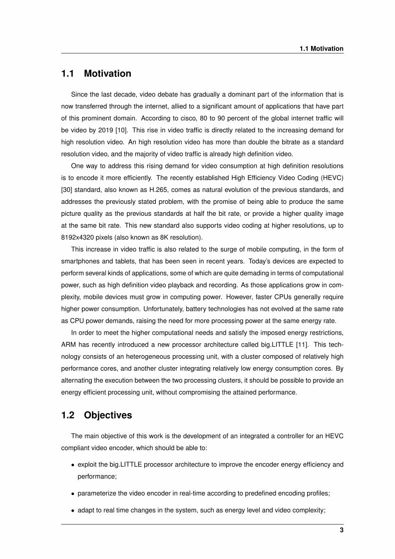
1.1 Motivation
1.1 Motivation
Since the last decade, video debate has gradually a dominant part of the information that is
now transferred through the internet, allied to a significant amount of applications that have part
of this prominent domain. According to cisco, 80 to 90 percent of the global internet traffic will
be video by 2019 [10]. This rise in video traffic is directly related to the increasing demand for
high resolution video. An high resolution video has more than double the bitrate as a standard
resolution video, and the majority of video traffic is already high definition video.
One way to address this rising demand for video consumption at high definition resolutions
is to encode it more efficiently. The recently established High Efficiency Video Coding (HEVC)
[30] standard, also known as H.265, comes as natural evolution of the previous standards, and
addresses the previously stated problem, with the promise of being able to produce the same
picture quality as the previous standards at half the bit rate, or provide a higher quality image
at the same bit rate. This new standard also supports video coding at higher resolutions, up to
8192x4320 pixels (also known as 8K resolution).
This increase in video traffic is also related to the surge of mobile computing, in the form of
smartphones and tablets, that has been seen in recent years. Today’s devices are expected to
perform several kinds of applications, some of which are quite demading in terms of computational
power, such as high definition video playback and recording. As those applications grow in com-
plexity, mobile devices must grow in computing power. However, faster CPUs generally require
higher power consumption. Unfortunately, battery technologies has not evolved at the same rate
as CPU power demands, raising the need for more processing power at the same energy rate.
In order to meet the higher computational needs and satisfy the imposed energy restrictions,
ARM has recently introduced a new processor architecture called big.LITTLE [11]. This tech-
nology consists of an heterogeneous processing unit, with a cluster composed of relatively high
performance cores, and another cluster integrating relatively low energy consumption cores. By
alternating the execution between the two processing clusters, it should be possible to provide an
energy efficient processing unit, without compromising the attained performance.
1.2 Objectives
The main objective of this work is the development of an integrated a controller for an HEVC
compliant video encoder, which should be able to:
• exploit the big.LITTLE processor architecture to improve the encoder energy efficiency and
performance;
• parameterize the video encoder in real-time according to predefined encoding profiles;
• adapt to real time changes in the system, such as energy level and video complexity;
3

1. Introduction
• meet predefined performance, energy, bitrate and video quality constraints;
• optimize the respective metrics according to the defined optimization profiles.
1.3 Main contributions
In this thesis, a control loop is proposed, which is able to parameterize an HEVC video encoder
as well as exploit the big.LITTLE processor. The controller enables the encoder parameterization
in real-time, allowing the video coding execution to comply with defined performance, energy ef-
ficiency, bitrate and video quality target thresholds. In addition, the proposed control algorithm
dynamically reacts to variations in the system, most commonly caused by the fluctuating com-
putational demands of the encoding video sequence, due to varying characteristics in the video
frames, such as high movement sequences followed by low movement sequences. The con-
troller presents a quick response time to these variations, adjusting the optimization parameters
according to the defined constraints and optimization profile.
Furthermore, this real-time adaption to the encoding video is also verified for the defined target
thresholds. This proves to be most relevant in mobile platforms, since its energy levels (i.e., energy
constraints) change over time, due to such factors as a depleting battery.
1.4 Dissertation outline
In the next chapter, we will expand upon video coding, focusing on the specifications of the
HEVC standard. Another crucial technology behind this work is the big.LITTLE technology, which
is explained in more detail in chapter 3. The next chapter will then contextualize this work by
presenting the state of the art in HEVC video coding using the big.LITTLE processor. In the fifth
chapter, we will focus on formalizing the problem we are addressing, as well as the proposed so-
lution. The sixth chapter will go into more detail about the implemented solution, while the seventh
chapter is dedicated to the presentation and discussion of the experimental results. Finally, the
last chapter of this work features the conclusions that we drew from the previous chapters, as well
as outlines for future work.
4
2High Efficiency Video Coding
Contents2.1 HEVC standard . . . . . . . . . . . . . . . . . . . . . . . . . . . . . . . . . . . . . 62.2 Parallelization approaches to video coding . . . . . . . . . . . . . . . . . . . . 112.3 State of the art HEVC software encoder: x265 . . . . . . . . . . . . . . . . . . . 182.4 Summary . . . . . . . . . . . . . . . . . . . . . . . . . . . . . . . . . . . . . . . . 21
5
2. High Efficiency Video Coding
2.1 HEVC standard
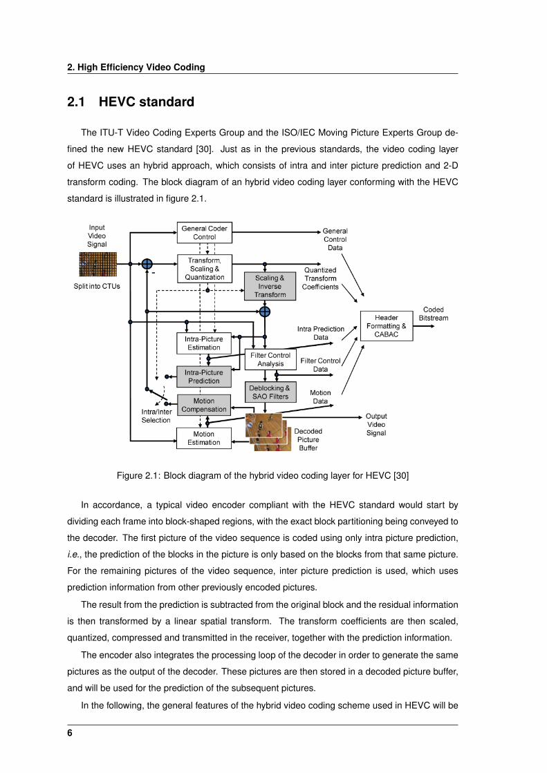
The ITU-T Video Coding Experts Group and the ISO/IEC Moving Picture Experts Group de-
fined the new HEVC standard [30]. Just as in the previous standards, the video coding layer
of HEVC uses an hybrid approach, which consists of intra and inter picture prediction and 2-D
transform coding. The block diagram of an hybrid video coding layer conforming with the HEVC
standard is illustrated in figure 2.1.
Figure 2.1: Block diagram of the hybrid video coding layer for HEVC [30]
In accordance, a typical video encoder compliant with the HEVC standard would start by
dividing each frame into block-shaped regions, with the exact block partitioning being conveyed to
the decoder. The first picture of the video sequence is coded using only intra picture prediction,
i.e., the prediction of the blocks in the picture is only based on the blocks from that same picture.
For the remaining pictures of the video sequence, inter picture prediction is used, which uses
prediction information from other previously encoded pictures.
The result from the prediction is subtracted from the original block and the residual information
is then transformed by a linear spatial transform. The transform coefficients are then scaled,
quantized, compressed and transmitted in the receiver, together with the prediction information.
The encoder also integrates the processing loop of the decoder in order to generate the same
pictures as the output of the decoder. These pictures are then stored in a decoded picture buffer,
and will be used for the prediction of the subsequent pictures.
In the following, the general features of the hybrid video coding scheme used in HEVC will be
6
2.1 HEVC standard
described in a little more detail.
2.1.1 Sampled Representation of Pictures
Video footage is typically captured using the RGB color space, which is not a particularity
efficient representation for video coding. On the contrary, HEVC uses a more video coding friendly
color space, the YCbCr, which divides the color space in 3 components: Y, known as luma,
representing brightness; Cb and Cr, also known as chroma, which represent how much color
deviates from gray towards blue and red, respectively. As the human visual system is more
sensitive to brightness, the typically used sampling scheme follows the 4:2:0 structure, meaning
that four luma components are sampled for every chroma component. HEVC also supports each
sample pixel value with 8 or 10 bits precision, with 8 bits being the most commonly used.
2.1.2 Subdivision of pictures
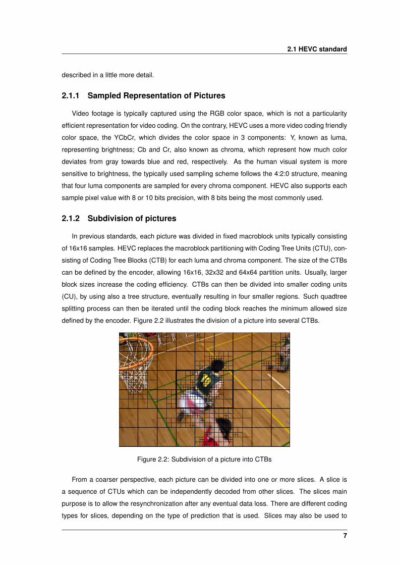
In previous standards, each picture was divided in fixed macroblock units typically consisting
of 16x16 samples. HEVC replaces the macroblock partitioning with Coding Tree Units (CTU), con-
sisting of Coding Tree Blocks (CTB) for each luma and chroma component. The size of the CTBs
can be defined by the encoder, allowing 16x16, 32x32 and 64x64 partition units. Usually, larger
block sizes increase the coding efficiency. CTBs can then be divided into smaller coding units
(CU), by using also a tree structure, eventually resulting in four smaller regions. Such quadtree
splitting process can then be iterated until the coding block reaches the minimum allowed size
defined by the encoder. Figure 2.2 illustrates the division of a picture into several CTBs.
Figure 2.2: Subdivision of a picture into CTBs
From a coarser perspective, each picture can be divided into one or more slices. A slice is
a sequence of CTUs which can be independently decoded from other slices. The slices main
purpose is to allow the resynchronization after any eventual data loss. There are different coding
types for slices, depending on the type of prediction that is used. Slices may also be used to
7
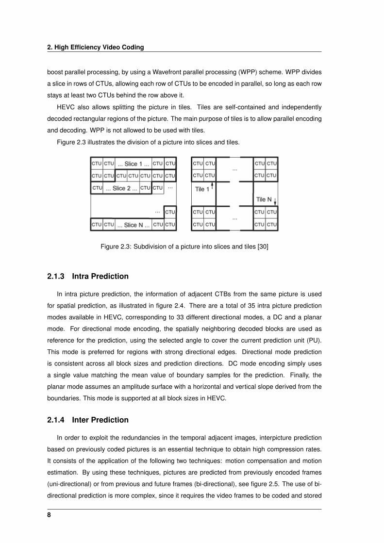
2. High Efficiency Video Coding
boost parallel processing, by using a Wavefront parallel processing (WPP) scheme. WPP divides
a slice in rows of CTUs, allowing each row of CTUs to be encoded in parallel, so long as each row
stays at least two CTUs behind the row above it.
HEVC also allows splitting the picture in tiles. Tiles are self-contained and independently
decoded rectangular regions of the picture. The main purpose of tiles is to allow parallel encoding
and decoding. WPP is not allowed to be used with tiles.
Figure 2.3 illustrates the division of a picture into slices and tiles.
Figure 2.3: Subdivision of a picture into slices and tiles [30]
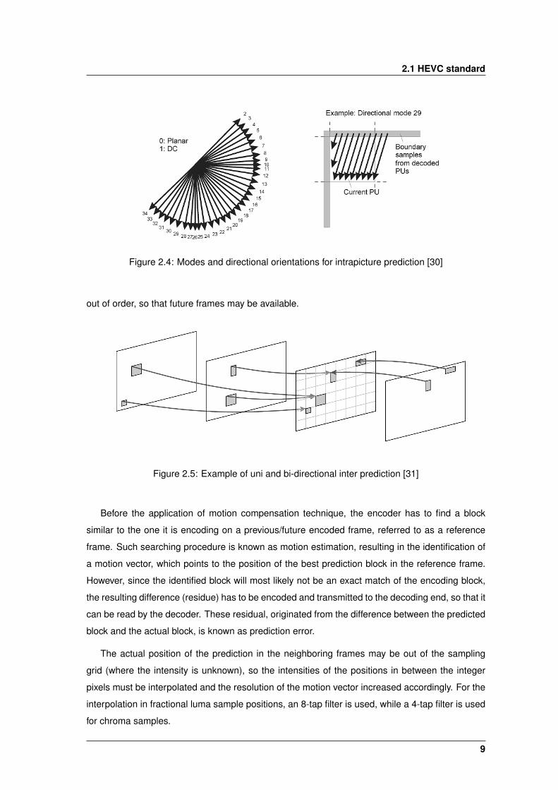
2.1.3 Intra Prediction
In intra picture prediction, the information of adjacent CTBs from the same picture is used
for spatial prediction, as illustrated in figure 2.4. There are a total of 35 intra picture prediction
modes available in HEVC, corresponding to 33 different directional modes, a DC and a planar
mode. For directional mode encoding, the spatially neighboring decoded blocks are used as
reference for the prediction, using the selected angle to cover the current prediction unit (PU).
This mode is preferred for regions with strong directional edges. Directional mode prediction
is consistent across all block sizes and prediction directions. DC mode encoding simply uses
a single value matching the mean value of boundary samples for the prediction. Finally, the
planar mode assumes an amplitude surface with a horizontal and vertical slope derived from the
boundaries. This mode is supported at all block sizes in HEVC.
2.1.4 Inter Prediction
In order to exploit the redundancies in the temporal adjacent images, interpicture prediction
based on previously coded pictures is an essential technique to obtain high compression rates.
It consists of the application of the following two techniques: motion compensation and motion
estimation. By using these techniques, pictures are predicted from previously encoded frames
(uni-directional) or from previous and future frames (bi-directional), see figure 2.5. The use of bi-
directional prediction is more complex, since it requires the video frames to be coded and stored
8
2.1 HEVC standard
Figure 2.4: Modes and directional orientations for intrapicture prediction [30]
out of order, so that future frames may be available.
Figure 2.5: Example of uni and bi-directional inter prediction [31]
Before the application of motion compensation technique, the encoder has to find a block
similar to the one it is encoding on a previous/future encoded frame, referred to as a reference
frame. Such searching procedure is known as motion estimation, resulting in the identification of
a motion vector, which points to the position of the best prediction block in the reference frame.
However, since the identified block will most likely not be an exact match of the encoding block,
the resulting difference (residue) has to be encoded and transmitted to the decoding end, so that it
can be read by the decoder. These residual, originated from the difference between the predicted
block and the actual block, is known as prediction error.
The actual position of the prediction in the neighboring frames may be out of the sampling
grid (where the intensity is unknown), so the intensities of the positions in between the integer
pixels must be interpolated and the resolution of the motion vector increased accordingly. For the
interpolation in fractional luma sample positions, an 8-tap filter is used, while a 4-tap filter is used
for chroma samples.
9
2. High Efficiency Video Coding
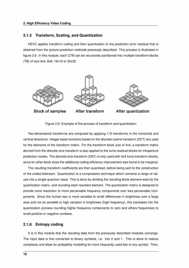
2.1.5 Transform, Scaling, and Quantization
HEVC applies transform coding and then quantization to the prediction error residual that is
obtained from the picture prediction methods previously described. This process is illustrated in
figure 2.6. In this module, each CTB can be recursively partitioned into multiple transform blocks
(TB) of size 4x4, 8x8, 16x16 or 32x32.
Figure 2.6: Example of the process of transform and quantization
Two-dimensional transforms are computed by applying 1-D transforms in the horizontal and
vertical directions. Integer basis functions based on the discrete cosine transform (DCT) are used
for the elements of the transform matrix. For the transform block size of 4x4, a transform matrix
derived from the discrete sine transform is also applied to the luma residual blocks for intrapicture
prediction modes. The discrete sine transform (DST) is only used with 4x4 luma transform blocks,
since for other block sizes the additional coding efficiency improvement was found to be marginal.
The resulting transform coefficients are then quantized, before being sent to the construction
of the coded bitstream. Quantization is a compression technique which converts a range of val-
ues into a single quantum value. This is done by dividing the resulting block element-wise by the
quantization matrix, and rounding each resultant element. The quantization matrix is designed to
provide more resolution to more perceivable frequency components over less perceivable com-
ponents. Since the human eye is more sensible to small differences in brightness over a large
area and not so sensible to high variation in brightness (high frequency), this translates into the
quantization process rounding higher frequency components to zero and others frequencies to
small positive or negative numbers.
2.1.6 Entropy coding
It is in this module that the resulting data from the previously described modules converge.
The input data is first converted to binary symbols, i.e. into 0 and 1. This is done to reduce
complexity and allow for probability modelling for more frequently used bits of any symbol. Then,
10

2.2 Parallelization approaches to video coding
an entropy coding technique is applied to compress the data and originate the output coded
bitstream. Context-adaptive binary arithmetic coding (CABAC) is the only entropy coding method
specified by the HEVC standard. CABAC is a lossless compression technique which is one of the
key factors for the levels of compressions allowed by HEVC.
2.1.7 In-Loop Filters
Before writing the samples in the decoded picture buffer, they are processed first by a deblock-
ing filter (DBF) and then by a sample adaptive offset filter (SAO).
Block based coding schemes tend to produce blocking artifacts due to the fact that inner blocks
are coded with more accuracy than outer blocks. To mitigate such artifacts, the decoded samples
are filtered by a DBF. After the deblocking has been processed, the samples are processed by
SAO, a filter designed to allow for better reconstruction of the original signal amplitudes, reducing
banding and ringing artifacts. SAO is performed on a per CTB basis and may or may not be
applied, depending on the filtering type selected.
2.1.8 Profiles
Profiles specify conformance points for implementing the standard in an inter-operable way
across various applications that have similar functional requirements. A profile defines a set of
coding tools that can be used when generating a conforming bitstream. An encoder for a given
profile may choose which coding tools to use, as long as it generates a conforming bitstream. In
contrast, a decoder compliant with a given profile must support all coding tools that can be used in
that profile. The first version of the HEVC standard defines three profiles: Main, Main 10 and Main
Still Picture [30]. The second version adds several new profiles, to a total of 27 different profiles.
New extensions include an increased bit depth (up to 12 bits), 4:2:2/4:4:4 chroma sampling, Mul-
tiview Video Coding and Scalable Video Coding. More recently, the third version of HEVC added
another 15 profiles, including one 3D profile, seven screen content coding extensions profiles,
three high throughput extensions profiles, and four scalable extensions profiles.
2.2 Parallelization approaches to video coding
HEVC video encoding is a complex task, several times more complex than encoding a H.264
video stream [7]. This increase in complexity is mainly due to the improvements that have been
introduced in picture prediction modules, modules which already represented the majority of the
encoding time for the H.264 standard.
With this observation in mind is important to focus on trying to achieve the maximum possible
performance in order to encode video streams in a timely fashion, and one way to do that is
through parallel processing.
11
2. High Efficiency Video Coding
2.2.1 Parallel Processing Platforms
Currently, there are several platforms which provide parallel computation. On this section, we
will focus on multicore CPUs, CPU clusters and GPUs.
A multicore CPU consists of a processing unit with several identical cores. The memory be-
tween cores is usually shared by the cores, with a dedicated L1 cache for each core. This allows
for a good parallelism, since the communication between cores has a low overhead. The main lim-
itation of this platform is the reduced number of cores available. For more memory and processor
demanding applications several CPUs may be used in the form of a CPU cluster.
A CPU cluster consists of several identical processing units. Each processing unit may have
several cores, and each has its own main memory. The main challenge in this platform is con-
cerned with the fact that each processing unit has its own non-shared memory, making the data
transfers between units quite slow. As a result, this kind of platform is more suited to compute
programs in which the computational demands overweight the data transfer requirements. Other
disadvantage to using cluster is that it is a (relatively) expensive platform, not available to the
typical user. A more accessible platform, which also allows for a high level of parallelism, is the
GPU.
GPUs are specifically made for computer graphics and image processing, although they can
also be used for general computing. A typical GPU has several hundred cores, making it a good
platform for highly parallelizable programs. However, each individual core is usually slower than
a typical CPU core, making the GPU only viable to compute tasks which can be divided into
a significant amount of threads. Furthermore, a GPU still needs a CPU for general purpose
computing and the communication overhead between them can be another handicap.
2.2.2 Parallel implementations of video coding
The HEVC video coding standard improves the encoding efficiency upon the H.264 while
maintaining the same strategy for the coding process. Consequently, many parallelization ap-
proaches that have been proposed for H.264 are still valid for HEVC. However the H.264 was
not defined by tuning its parallelization in mind, thus posing difficult constraints to achieve greater
performance levels. Even so, the most used parallelization approaches in H.264 involve the ex-
ploitation of Group-of-Pictures-level (GOP-level) parallelism, frame-level paralellism, slice-level
parallelism and macroblock-level parallelism. Macroblock-level parallelism will not be discussed
in this document since it does not translate well to HEVC.
In contrast, HEVC was designed by allowing the exploitation of more parallelization opportuni-
ties, to the definition of improves on the parallelization approach of H.264, using mainly two new
tools: WPP and tiles. These tools allow for the subdivision of each picture into multiple partitions
that can be independently processed in parallel. Each partition contains an integer number of
CTB, that may or may not have dependencies on other partitions.
12
2.2 Parallelization approaches to video coding
2.2.2.A GOP-level Parallelism
This is the most popular approach to parallelize the video coding procedure since it is relatively
simple and easy to implement. In GOP-level parallelism, each GOP is handled by a separate
thread. To allow for parallelism, this method uses temporal division of frames. Consequently,
dependency exits among the frames within a GOP but no data dependency exists between two
sets of GOPs, thus allowing for each GOP to be independently processed. The main limitation
to this approach is the imposed coding latency, which does not allow this approach to achieve
real time encoding. Another limitation is the memory access. Since typical caches are insufficient
to store several frames, this parallelization approach leads to a lot of accesses to main memory,
effectively limiting the potential performance improvements.
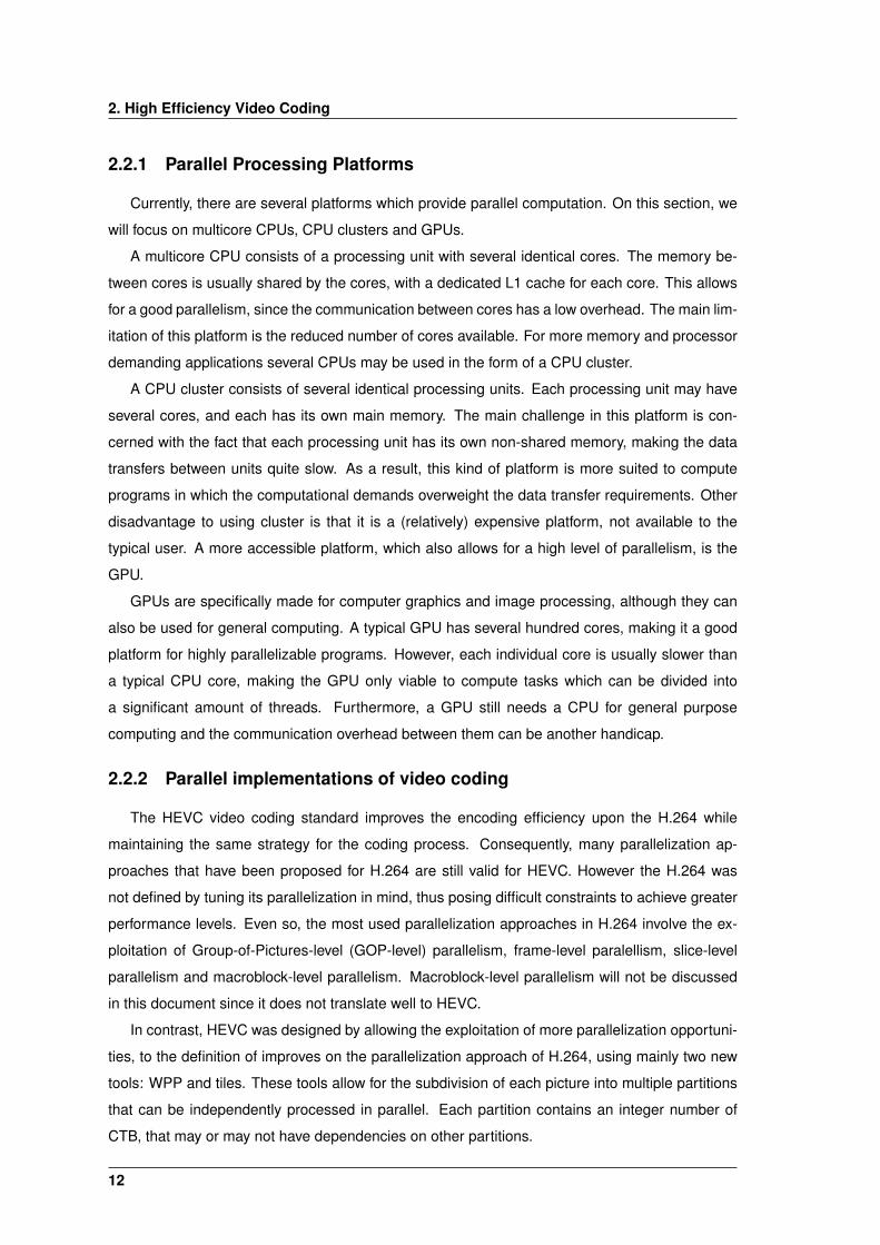
Sankaraiah et al. [29] explored GOP-level parallelism in H.264 video encoding on multicore
platforms. The obtained results for a quad core processor with varying GOP size are summarized
in Figure 2.7. From these figures we note that a GOP size 15 yields the optimum results regard
to these quality parameters.
(a) Encoding time vs GOP size (b) Bit-rate vs GOP size
Figure 2.7: Variation of encoding time and bit-rate with GOP size [29]
2.2.2.B Frame-level Parallelism
Frame-level parallelism consists of coding several frames of the same GOP at the same time,
provided that the motion compensation dependences are satisfied. There are, however, a number
of limitations to this approach. It depends on the availability of other encoding frames, used as
reference frames for motion estimation. While this reference frames are not fully encoded and
available, the encoding frame thread will be forced to idly wait. Its also hard to properly balance
the workload between all cores since each frame may take a different time to encode. Also worth
noting that this parallelization strategy does not improve the frame latency, only the frame rate.
13
2. High Efficiency Video Coding
2.2.2.C Slice-level Parallelism
As in H.264 and most current hybrid video coding standards, HEVC allows for each frame to
be divided in several slices, in order to add robustness to the bitstream. Each slice is completely
independent from each other, providing a further opportunity for parallel processing. There are
some problems with slice-level parallelism though. In-loop filters are applied across slice bound-
aries, reducing the advantage of having independent slices. The number of slices also reduces
the coding efficiency significantly. Due to these reasons, exploiting slice-level parallelism is only
advisable when there are few slices per frame.
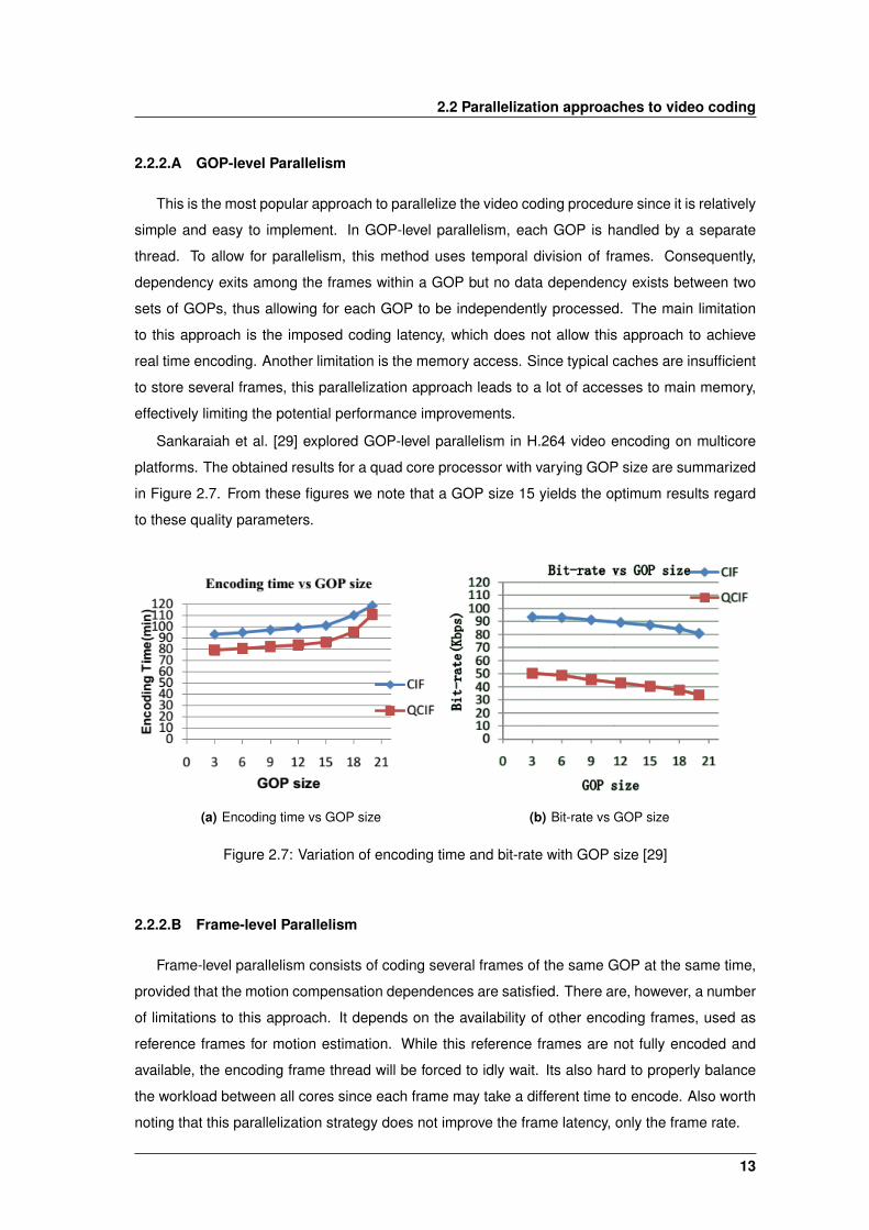
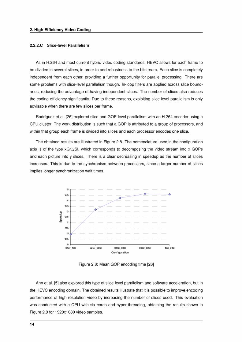
Rodrıguez et al. [26] explored slice and GOP-level parallelism with an H.264 encoder using a
CPU cluster. The work distribution is such that a GOP is attributed to a group of processors, and
within that group each frame is divided into slices and each processor encodes one slice.
The obtained results are illustrated in Figure 2.8. The nomenclature used in the configuration
axis is of the type xGr ySl, which corresponds to decomposing the video stream into x GOPs
and each picture into y slices. There is a clear decreasing in speedup as the number of slices
increases. This is due to the synchronism between processors, since a larger number of slices
implies longer synchronization wait times.
Figure 2.8: Mean GOP encoding time [26]
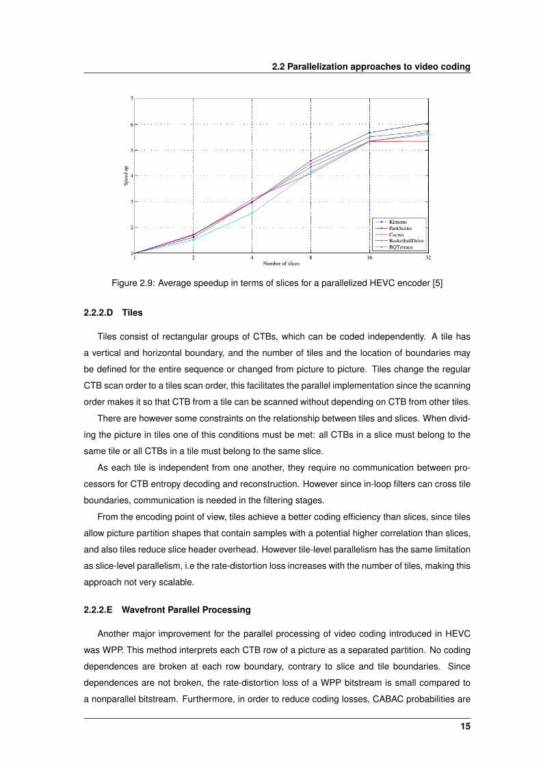
Ahn et al. [5] also explored this type of slice-level parallelism and software acceleration, but in
the HEVC encoding domain. The obtained results illustrate that it is possible to improve encoding
performance of high resolution video by increasing the number of slices used. This evaluation
was conducted with a CPU with six cores and hyper-threading, obtaining the results shown in
Figure 2.9 for 1920x1080 video samples.
14
2.2 Parallelization approaches to video coding
Figure 2.9: Average speedup in terms of slices for a parallelized HEVC encoder [5]
2.2.2.D Tiles
Tiles consist of rectangular groups of CTBs, which can be coded independently. A tile has
a vertical and horizontal boundary, and the number of tiles and the location of boundaries may
be defined for the entire sequence or changed from picture to picture. Tiles change the regular
CTB scan order to a tiles scan order, this facilitates the parallel implementation since the scanning
order makes it so that CTB from a tile can be scanned without depending on CTB from other tiles.
There are however some constraints on the relationship between tiles and slices. When divid-
ing the picture in tiles one of this conditions must be met: all CTBs in a slice must belong to the
same tile or all CTBs in a tile must belong to the same slice.
As each tile is independent from one another, they require no communication between pro-
cessors for CTB entropy decoding and reconstruction. However since in-loop filters can cross tile
boundaries, communication is needed in the filtering stages.
From the encoding point of view, tiles achieve a better coding efficiency than slices, since tiles
allow picture partition shapes that contain samples with a potential higher correlation than slices,
and also tiles reduce slice header overhead. However tile-level parallelism has the same limitation
as slice-level parallelism, i.e the rate-distortion loss increases with the number of tiles, making this
approach not very scalable.
2.2.2.E Wavefront Parallel Processing
Another major improvement for the parallel processing of video coding introduced in HEVC
was WPP. This method interprets each CTB row of a picture as a separated partition. No coding
dependences are broken at each row boundary, contrary to slice and tile boundaries. Since
dependences are not broken, the rate-distortion loss of a WPP bitstream is small compared to
a nonparallel bitstream. Furthermore, in order to reduce coding losses, CABAC probabilities are
15
2. High Efficiency Video Coding
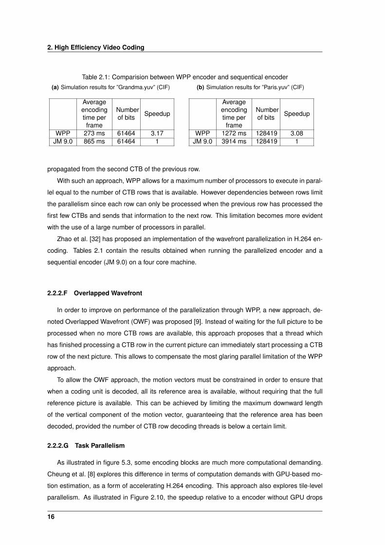
Table 2.1: Comparision between WPP encoder and sequentical encoder(a) Simulation results for ”Grandma.yuv” (CIF)
Averageencodingtime perframe
Numberof bits Speedup
WPP 273 ms 61464 3.17JM 9.0 865 ms 61464 1
(b) Simulation results for ”Paris.yuv” (CIF)
Averageencodingtime perframe
Numberof bits Speedup
WPP 1272 ms 128419 3.08JM 9.0 3914 ms 128419 1
propagated from the second CTB of the previous row.
With such an approach, WPP allows for a maximum number of processors to execute in paral-
lel equal to the number of CTB rows that is available. However dependencies between rows limit
the parallelism since each row can only be processed when the previous row has processed the
first few CTBs and sends that information to the next row. This limitation becomes more evident
with the use of a large number of processors in parallel.
Zhao et al. [32] has proposed an implementation of the wavefront parallelization in H.264 en-
coding. Tables 2.1 contain the results obtained when running the parallelized encoder and a
sequential encoder (JM 9.0) on a four core machine.
2.2.2.F Overlapped Wavefront
In order to improve on performance of the parallelization through WPP, a new approach, de-
noted Overlapped Wavefront (OWF) was proposed [9]. Instead of waiting for the full picture to be
processed when no more CTB rows are available, this approach proposes that a thread which
has finished processing a CTB row in the current picture can immediately start processing a CTB
row of the next picture. This allows to compensate the most glaring parallel limitation of the WPP
approach.
To allow the OWF approach, the motion vectors must be constrained in order to ensure that
when a coding unit is decoded, all its reference area is available, without requiring that the full
reference picture is available. This can be achieved by limiting the maximum downward length
of the vertical component of the motion vector, guaranteeing that the reference area has been
decoded, provided the number of CTB row decoding threads is below a certain limit.
2.2.2.G Task Parallelism
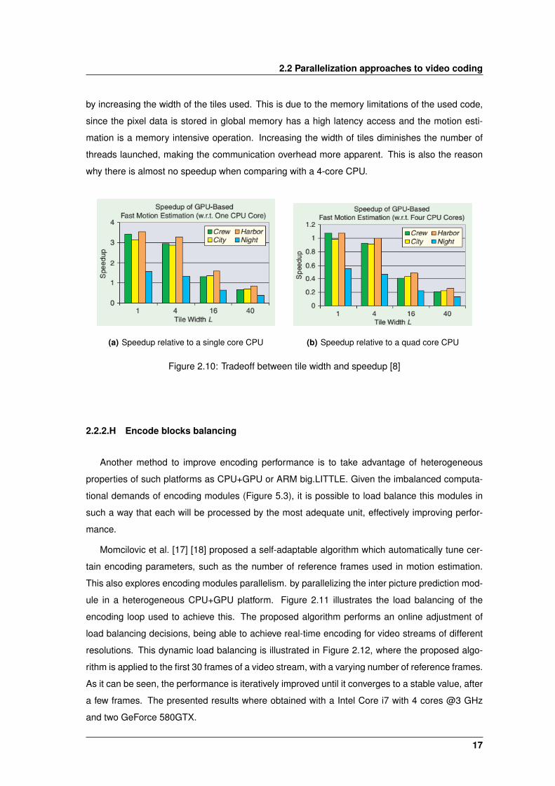
As illustrated in figure 5.3, some encoding blocks are much more computational demanding.
Cheung et al. [8] explores this difference in terms of computation demands with GPU-based mo-
tion estimation, as a form of accelerating H.264 encoding. This approach also explores tile-level
parallelism. As illustrated in Figure 2.10, the speedup relative to a encoder without GPU drops
16
2.2 Parallelization approaches to video coding
by increasing the width of the tiles used. This is due to the memory limitations of the used code,
since the pixel data is stored in global memory has a high latency access and the motion esti-
mation is a memory intensive operation. Increasing the width of tiles diminishes the number of
threads launched, making the communication overhead more apparent. This is also the reason
why there is almost no speedup when comparing with a 4-core CPU.
(a) Speedup relative to a single core CPU (b) Speedup relative to a quad core CPU
Figure 2.10: Tradeoff between tile width and speedup [8]
2.2.2.H Encode blocks balancing
Another method to improve encoding performance is to take advantage of heterogeneous
properties of such platforms as CPU+GPU or ARM big.LITTLE. Given the imbalanced computa-
tional demands of encoding modules (Figure 5.3), it is possible to load balance this modules in
such a way that each will be processed by the most adequate unit, effectively improving perfor-
mance.
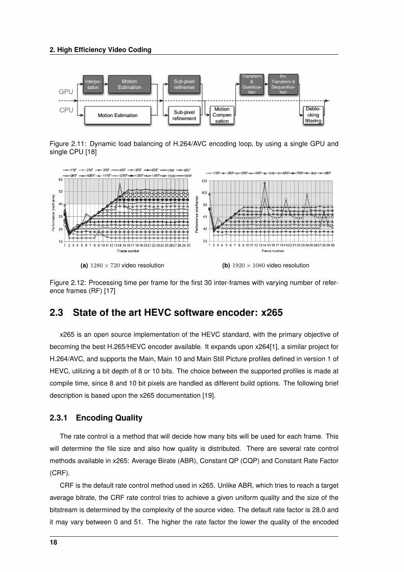
Momcilovic et al. [17] [18] proposed a self-adaptable algorithm which automatically tune cer-
tain encoding parameters, such as the number of reference frames used in motion estimation.
This also explores encoding modules parallelism. by parallelizing the inter picture prediction mod-
ule in a heterogeneous CPU+GPU platform. Figure 2.11 illustrates the load balancing of the
encoding loop used to achieve this. The proposed algorithm performs an online adjustment of
load balancing decisions, being able to achieve real-time encoding for video streams of different
resolutions. This dynamic load balancing is illustrated in Figure 2.12, where the proposed algo-
rithm is applied to the first 30 frames of a video stream, with a varying number of reference frames.
As it can be seen, the performance is iteratively improved until it converges to a stable value, after
a few frames. The presented results where obtained with a Intel Core i7 with 4 cores @3 GHz
and two GeForce 580GTX.
17
2. High Efficiency Video Coding
Figure 2.11: Dynamic load balancing of H.264/AVC encoding loop, by using a single GPU andsingle CPU [18]
(a) 1280× 720 video resolution (b) 1920× 1080 video resolution
Figure 2.12: Processing time per frame for the first 30 inter-frames with varying number of refer-ence frames (RF) [17]
2.3 State of the art HEVC software encoder: x265
x265 is an open source implementation of the HEVC standard, with the primary objective of
becoming the best H.265/HEVC encoder available. It expands upon x264[1], a similar project for
H.264/AVC, and supports the Main, Main 10 and Main Still Picture profiles defined in version 1 of
HEVC, utilizing a bit depth of 8 or 10 bits. The choice between the supported profiles is made at
compile time, since 8 and 10 bit pixels are handled as different build options. The following brief
description is based upon the x265 documentation [19].
2.3.1 Encoding Quality
The rate control is a method that will decide how many bits will be used for each frame. This
will determine the file size and also how quality is distributed. There are several rate control
methods available in x265: Average Birate (ABR), Constant QP (CQP) and Constant Rate Factor
(CRF).
CRF is the default rate control method used in x265. Unlike ABR, which tries to reach a target
average bitrate, the CRF rate control tries to achieve a given uniform quality and the size of the
bitstream is determined by the complexity of the source video. The default rate factor is 28.0 and
it may vary between 0 and 51. The higher the rate factor the lower the quality of the encoded
18
2.3 State of the art HEVC software encoder: x265
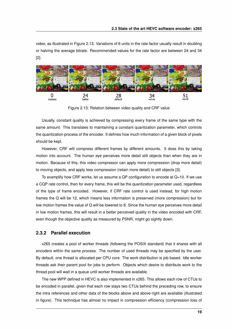
video, as illustrated in Figure 2.13. Variations of 6 units in the rate factor usually result in doubling
or halving the average bitrate. Recommended values for the rate factor are between 24 and 34
[2].
Figure 2.13: Relation between video quality and CRF value
Usually, constant quality is achieved by compressing every frame of the same type with the
same amount. This translates to maintaining a constant quantization parameter, which controls
the quantization process of the encoder. It defines how much information of a given block of pixels
should be kept.
However, CRF will compress different frames by different amounts. It does this by taking
motion into account. The human eye perceives more detail still objects than when they are in
motion. Because of this, this video compressor can apply more compression (drop more detail)
to moving objects, and apply less compression (retain more detail) to still objects [3].
To examplify how CRF works, let us assume a QP configuration to encode at Q=10. If we use
a CQP rate control, then for every frame, this will be the quantization parameter used, regardless
of the type of frame encoded. However, if CRF rate control is used instead, for high motion
frames the Q will be 12, which means less information is preserved (more compression) but for
low motion frames the value of Q will be lowered to 8. Since the human eye perceives more detail
in low motion frames, this will result in a better perceived quality in the video encoded with CRF,
even though the objective quality as measured by PSNR, might go sightly down.
2.3.2 Parallel execution
x265 creates a pool of worker threads (following the POSIX standard) that it shares with all
encoders within the same process. The number of used threads may be specified by the user.
By default, one thread is allocated per CPU core. The work distribution is job based. Idle worker
threads ask their parent pool for jobs to perform. Objects which desire to distribute work to the
thread pool will wait in a queue until worker threads are available.
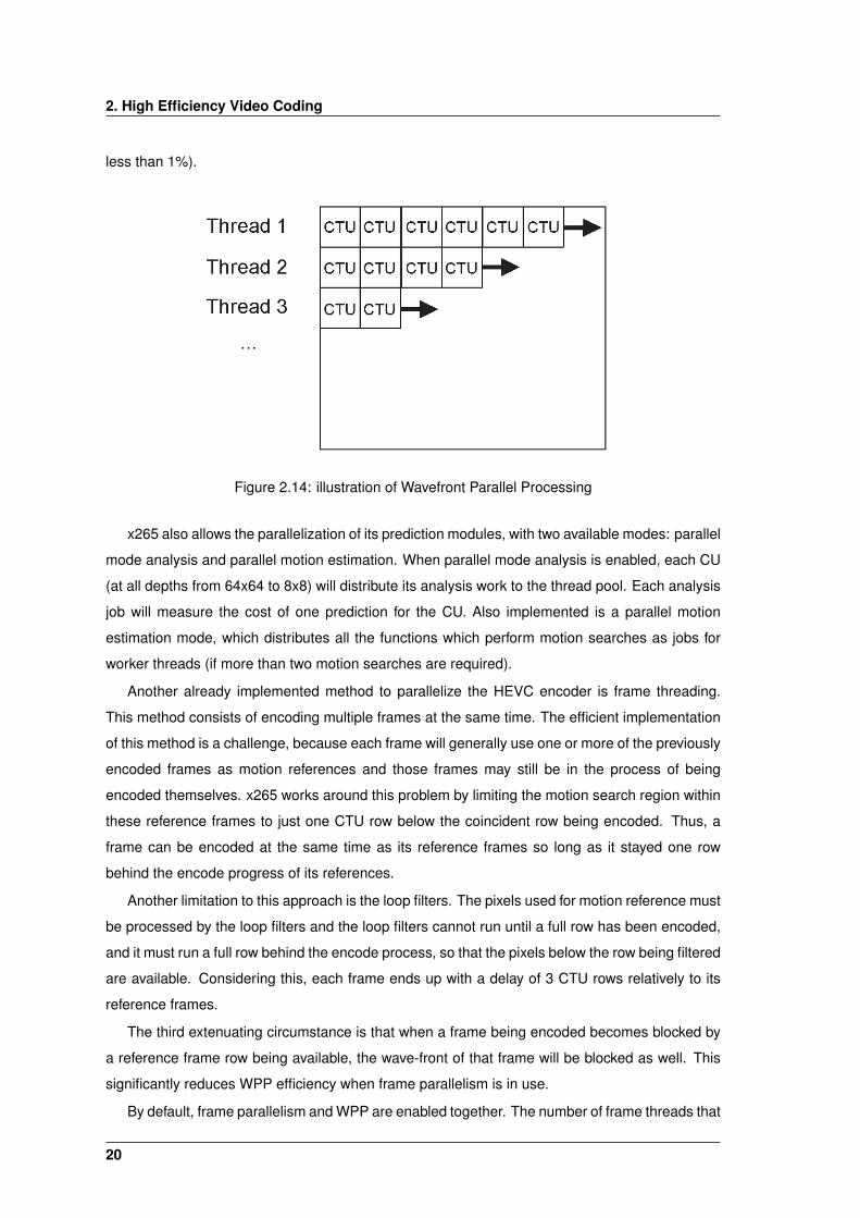
The new WPP defined in HEVC is also implemented in x265. This allows each row of CTUs to
be encoded in parallel, given that each row stays two CTUs behind the preceding row, to ensure
the intra references and other data of the blocks above and above-right are available (illustrated
in figure). This technique has almost no impact in compression efficiency (compression loss of
19
2. High Efficiency Video Coding
less than 1%).
Figure 2.14: illustration of Wavefront Parallel Processing
x265 also allows the parallelization of its prediction modules, with two available modes: parallel
mode analysis and parallel motion estimation. When parallel mode analysis is enabled, each CU
(at all depths from 64x64 to 8x8) will distribute its analysis work to the thread pool. Each analysis
job will measure the cost of one prediction for the CU. Also implemented is a parallel motion
estimation mode, which distributes all the functions which perform motion searches as jobs for
worker threads (if more than two motion searches are required).
Another already implemented method to parallelize the HEVC encoder is frame threading.
This method consists of encoding multiple frames at the same time. The efficient implementation
of this method is a challenge, because each frame will generally use one or more of the previously
encoded frames as motion references and those frames may still be in the process of being
encoded themselves. x265 works around this problem by limiting the motion search region within
these reference frames to just one CTU row below the coincident row being encoded. Thus, a
frame can be encoded at the same time as its reference frames so long as it stayed one row
behind the encode progress of its references.
Another limitation to this approach is the loop filters. The pixels used for motion reference must
be processed by the loop filters and the loop filters cannot run until a full row has been encoded,
and it must run a full row behind the encode process, so that the pixels below the row being filtered
are available. Considering this, each frame ends up with a delay of 3 CTU rows relatively to its
reference frames.
The third extenuating circumstance is that when a frame being encoded becomes blocked by
a reference frame row being available, the wave-front of that frame will be blocked as well. This
significantly reduces WPP efficiency when frame parallelism is in use.
By default, frame parallelism and WPP are enabled together. The number of frame threads that
20
2.4 Summary
is used is auto-detected from the CPU logic core count, but may be also be manually specified.
The inferred frame threads, by number of cores, is as follows: 2 frames threads with at least
4 cores; 3 for at least 8 cores; 5 for at least 16 cores; and 6 for at least 32 cores. If WPP is
disabled, then the frame thread count defaults to the minimum between the number of cores
and half the number of CTU rows. This limitation is due to the previously mentioned restriction:
to encode several frames in parallel, the encoded frame must remain one CTU row behind the
encode process of its references.
When manually allocating frame threads, it is very important to not over-allocate them. Each
frame thread allocates a large amount of memory and because of the limited number of CTU rows
and the reference lag, there usually is no benefit to allocating above the detected count.
The described parallelization approaches aim at improving the encoding performance and the
presented considerations only regard homogeneous architectures. With this in mind, it may be
sensible to evaluate how these techniques perform in an heterogeneous architecture, such as the
ARM big.LITTLE, and alter thread scheduling accordingly. This modifications may not only be
performed to improve the encoding performance, but rather to improve its energy efficiency.
2.4 Summary
HEVC is a video coding standard defined by ITU-T Video Coding Experts Group and the
ISO/IEC Moving Picture Experts Group in 2013. It was introduced as a successor to the H.264/AVC
standard, improving upon coding efficiency, at the cost of computational power.
Similarly to previous standards, HEVC defines a hybrid video coding layer. The encoding
process starts by dividing the input picture into 64x64 blocks, denominated CTU, which may then
be further divided up to 8x8 blocks. In order to exploit spacial redundancy within the encoding
frame, intrapicture prediction is applied which uses neighboring pixels as references. Additionally,
interpicture prediction is also applied, as a way to exploit temporal redundancy between frames.
The difference between the original frame and the resulting frame after the mentioned prediction
processes will result in a residual, which is then transformed, scaled and quantized. The result is
then compress through entropy coding, that produces the final encoded bitstream.
There are several approaches to exploit the parallel execution of a video encoder compliant
with HEVC. In this chapter, we described the following: GOP-level parallelism, frame-level par-
allelism, slice-level parallelism, tiles, wavefront parallel processing, overlapped wavefront, task
parallelism and encode blocks balancing.
x265 is the video encoder software used in the development of this work. It provides an open
source solution which aims at providing the best HEVC compliant video encoder. We describe
the available encoding quality control and parallelization techniques implemented in this encoder.
21

2. High Efficiency Video Coding
22

3ARM big.LITTLE technology
Contents3.1 Software execution models for big.LITTLE . . . . . . . . . . . . . . . . . . . . 253.2 Cluster and CPU Migration . . . . . . . . . . . . . . . . . . . . . . . . . . . . . . 253.3 Global Task Scheduling . . . . . . . . . . . . . . . . . . . . . . . . . . . . . . . 273.4 Performance analysis . . . . . . . . . . . . . . . . . . . . . . . . . . . . . . . . . 293.5 Summary . . . . . . . . . . . . . . . . . . . . . . . . . . . . . . . . . . . . . . . . 30
23
3. ARM big.LITTLE technology
The ARM big.LITTLE processor technology was designed to provide high processing power
while still maintaining a low power consumption. This is achieved by using an asymmetric multi-
core CPU, with “big” cores providing the maximum processing power (while meeting power con-
straints) and “LITTLE” cores providing the maximum energy efficiency. Both big and LITTLE
processors are coherent and implement the same instruction set architecture (ISA), allowing to
dynamically migrate tasks between cores according to the demanded computational power.
Although both processor types support the same ARMv7-A ISA, they have different micro-
architectures, which allow them to offer different power and performance characteristics. The
LITTLE core is an in-order processor, having a simple pipeline with 8 processing stages that
provides an energy efficient processing capability. Even though the LITTLE core performance is
lower than the big core performance, it still provides enough processing power to satisfy most
usage scenarios in modern mobile devices. The big core is an out-order processor, with a multi-
issue pipeline that allows for several instructions to run in parallel, in order to a achieve higher
performance.
Until the date of writing, ARM has developed two generations of big.LITTLE processors. The
first generation uses a Cortex-A7 cluster for LITTLE and Cortex-A15 cluster for big, and supports
a 32-bit architecture (ARMv7). For the second generation, Cortex-A53 and Cortex-A57 processor
architectures are used, in which Cortex-A57 is the big processor cluster and Cortex-A53 the
LITTLE, both using a 64-bit architecture (ARMv8).
Contrasting to other architectures, this CPU exploits the fact that the instantaneous perfor-
mance requirement of most applications varies greatly during its execution. Most tasks will run
on a LITTLE core, and only tasks that are too demanding for the LITTLE cores are migrated to
one or several big cores. When the computational requirements drop, then the task is migrated
to the LITTLE cores. The not used big cores can then be powered down, quickly reducing power
consumption. This allows for a energy efficient computation, without sacrificing performance.
For this technique to allow for any kind of power saving, task transitions between different
processors should be as smooth as possible, which is possible thanks to the coherency between
big and LITTLE cores. Without hardware coherency, the transfer of data between big and LITTLE
cores would occur through main memory, a slow and not energy efficient process. To enable a
seamless data transfer between clusters, a set of system fabric components, referred as “Cache
Coherent Interconnect”, is provided, in addition to a system which provides dynamically config-
urable interrupt distribution to all the cores (CoreLink GIC-400). This allows interrupts to be mi-
grated between any cores in the two clusters, which in conjunction with cache coherency, enables
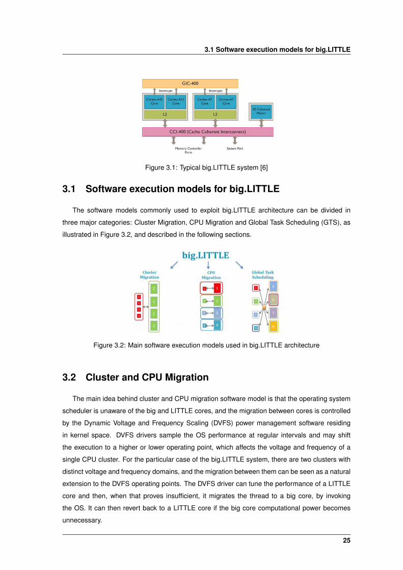
task migration between clusters. An example is illustrated in Figure 3.1 [25].
24
3.1 Software execution models for big.LITTLE
Figure 3.1: Typical big.LITTLE system [6]
3.1 Software execution models for big.LITTLE
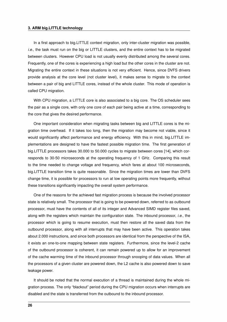
The software models commonly used to exploit big.LITTLE architecture can be divided in
three major categories: Cluster Migration, CPU Migration and Global Task Scheduling (GTS), as
illustrated in Figure 3.2, and described in the following sections.
Figure 3.2: Main software execution models used in big.LITTLE architecture
3.2 Cluster and CPU Migration
The main idea behind cluster and CPU migration software model is that the operating system
scheduler is unaware of the big and LITTLE cores, and the migration between cores is controlled
by the Dynamic Voltage and Frequency Scaling (DVFS) power management software residing
in kernel space. DVFS drivers sample the OS performance at regular intervals and may shift
the execution to a higher or lower operating point, which affects the voltage and frequency of a
single CPU cluster. For the particular case of the big.LITTLE system, there are two clusters with
distinct voltage and frequency domains, and the migration between them can be seen as a natural
extension to the DVFS operating points. The DVFS driver can tune the performance of a LITTLE
core and then, when that proves insufficient, it migrates the thread to a big core, by invoking
the OS. It can then revert back to a LITTLE core if the big core computational power becomes
unnecessary.
25
3. ARM big.LITTLE technology
In a first approach to big.LITTLE context migration, only inter-cluster migration was possible,
i.e., the task must run on the big or LITTLE clusters, and the entire context has to be migrated
between clusters. However CPU load is not usually evenly distributed among the several cores.
Frequently, one of the cores is experiencing a high load but the other cores in the cluster are not.
Migrating the entire context in these situations is not very efficient. Hence, since DVFS drivers
provide analysis at the core level (not cluster level), it makes sense to migrate to the context
between a pair of big and LITTLE cores, instead of the whole cluster. This mode of operation is
called CPU migration.
With CPU migration, a LITTLE core is also associated to a big core. The OS scheduler sees
the pair as a single core, with only one core of each pair being active at a time, corresponding to
the core that gives the desired performance.
One important consideration when migrating tasks between big and LITTLE cores is the mi-
gration time overhead. If it takes too long, then the migration may become not viable, since it
would significantly affect performance and energy efficiency. With this in mind, big.LITTLE im-
plementations are designed to have the fastest possible migration time. The first generation of
big.LITTLE processors takes 30.000 to 50.000 cycles to migrate between cores [14], which cor-
responds to 30-50 microseconds at the operating frequency of 1 GHz. Comparing this result
to the time needed to change voltage and frequency, which fares at about 100 microseconds,
big.LITTLE transition time is quite reasonable. Since the migration times are lower than DVFS
change time, it is possible for processors to run at low operating points more frequently, without
these transitions significantly impacting the overall system performance.
One of the reasons for the achieved fast migration process is because the involved processor
state is relatively small. The processor that is going to be powered down, referred to as outbound
processor, must have the contents of all of its integer and Advanced SIMD register files saved,
along with the registers which maintain the configuration state. The inbound processor, i.e., the
processor which is going to resume execution, must then restore all the saved data from the
outbound processor, along with all interrupts that may have been active. This operation takes
about 2.000 instructions, and since both processors are identical from the perspective of the ISA,
it exists an one-to-one mapping between state registers. Furthermore, since the level-2 cache
of the outbound processor is coherent, it can remain powered up to allow for an improvement
of the cache warming time of the inbound processor through snooping of data values. When all
the processors of a given cluster are powered down, the L2 cache is also powered down to save
leakage power.
It should be noted that the normal execution of a thread is maintained during the whole mi-
gration process. The only “blackout” period during the CPU migration occurs when interrupts are
disabled and the state is transferred from the outbound to the inbound processor.
26
3.3 Global Task Scheduling
3.3 Global Task Scheduling
The execution model based on cluster or CPU migration limits the number of cores that can
be powered up at any given time, since the big and LITTLE cores are paired together. With global
task scheduling (GTS), the operating system is aware of the heterogeneous processors and it is
possible to have all of them running tasks at the same time. This also allows for less restrictions
when design the big.LITTLE processor, with an equal number of big and LITTLE cores no longer
required. This type of scheduling tracks the computational requirements of each individual thread
and the current load state of each processor, and uses this information to determine the optimal
balance of threads between big and LITTLE processors. Any unused processor is powered down.
If all the processors in a cluster are powered down, then the cluster itself is powered down too.
This scheduling system allows to reserve the big cluster for the exclusive use of intensive
threads, while other threads run on the LITTLE cluster. In contrast, with cluster and CPU mi-
gration, all the threads in a processor are transfered together, not allowing to isolate the most
demanding thread and thus achieving a slower completion time for heavy compute tasks. An-
other improvement of global task scheduling over CPU migration is the ability to target interrupts
individually to big or LITTLE cores. On the contrary, the CPU migration model assumes that the
whole context, including interrupt targeting, migrates between big and LITTLE processors.
In the whole, this scheduling method is considered a major improvement over cluster and
CPU migration, since it enables threads to be executed on the processing resource that is most
appropriate. As such, global task management shall be the focal point of all future development.
ARM implementation of GTS is known as big.LITTLE MP.
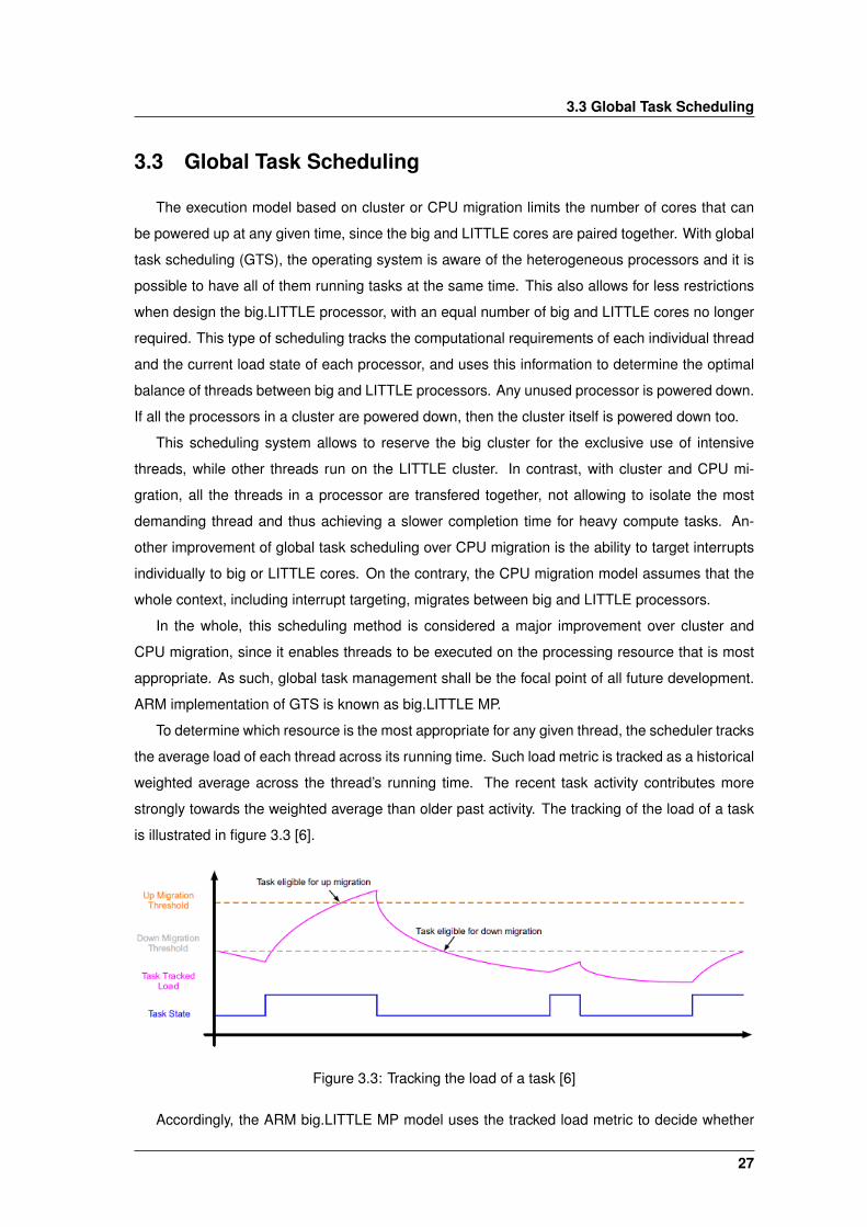
To determine which resource is the most appropriate for any given thread, the scheduler tracks
the average load of each thread across its running time. Such load metric is tracked as a historical
weighted average across the thread’s running time. The recent task activity contributes more
strongly towards the weighted average than older past activity. The tracking of the load of a task
is illustrated in figure 3.3 [6].
Figure 3.3: Tracking the load of a task [6]
Accordingly, the ARM big.LITTLE MP model uses the tracked load metric to decide whether
27
3. ARM big.LITTLE technology
and when to allocate a thread to a big or LITTLE core. This is done using two configurable
thresholds: the ”up migration threshold” and the ”down migration threshold”. When the tracked
load average of a thread, running on a LITTLE core, exceeds the up migration threshold, the
thread becomes eligible to be migrated to a big processor. The same logic is also true for threads
running on big cores, when the tracked load average goes below the down migration threshold,
making the thread to become eligible to migrate to a LITTLE core. These rules apply when
migrating between big and LITTLE cores. Within the clusters, standard Linux scheduler load
balancing applies, which tries to keep the load balanced across all cores in one cluster.
This model is further refined by adjusting the current operating frequency of each processor to
the tracked load metric. A task that is running when the processor is operated at half speed, will
accumulate tracked load at half the rate than it would if the processor was running at full speed.
This allows big.LITTLE MP and DVFS management to work together in harmony.
Under this assumption, the ARM big.LITTLE MP mode uses a number of software thread
affinity management techniques to determine when to migrate a task between big and LITTLE
processors: wake migration, fork migration, forced migration, idle-pull migration and offload mi-
gration.
Wake migration handles previously idle threads to now become ready to execute. To choose
between big and LITTLE cores, the scheduler uses the tracked load history of a task, generally
assuming that the task will resume on the same cluster as before. This is mainly due to the fact
that the load metric does not get updated when the task is idle. Upon waking up, the load metric
is the same as it was when the task went to sleep. To actually wake up in a different cluster, the
task must change its behavior before going to sleep. Rules are defined which ensure that big
cores generally only run a single intensive thread and run it to completion, so upward migration
only occurs to big cores which are idle. When migrating downwards, this rule does not apply and
multiple software threads may be allocated to a little core.
The fork migration, as the name implies, operates when the fork system call is used to create
a new thread. Since the thread is new, there is no historical data so the system defaults to
a big processor, on the basis that a light thread will quickly migrate to a LITTLE core. This
approach benefits compute heavy tasks without being expensive, since low intensity threads are
only running in a big core at creation time, quickly migrating to a LITTLE core thereafter. This also
assures that compute heavy threads are not penalized for getting launched in a LITTLE core.
Forced migration handles threads which do not sleep or rarely sleep. It periodically checks if
any thread running on a LITTLE core have crossed the up migration threshold, in which case it is
migrated to a big core.
Idle pull migration ensures the best use of active big cores. When a big core has no task to run,
it checks if any of the threads running on the LITTLE cluster is above the up migration threshold.
In such condition, it is quickly migrated to the idle big core. If no such thread is found, then the big
28
3.4 Performance analysis
core is powered down. This ensures that active big cores always take the most intensive task in
the system and run it until its completion. Furthermore, it greatly improves performance and the
energy efficiency of the system [6].
The big.LITTLE MP mode requires the normal scheduler load balancing to be disabled. This
can cause long running threads to concentrate on big cores and leave LITTLE cores idle or under-
utilized. It also implies that big.LITTLE computational power may be underutilized in tasks that
demand the maximum possible computation power. Offload migration addresses this issue by
periodically migrating threads to LITTLE cores to exploit unused compute capacity. Threads mi-
grated this way still remain candidates to up migration, if they exceed the up migration threshold.
3.4 Performance analysis
As discussed above, when compared with the first generation, the big.LITTLE MP scheduling
model has several improvements in terms of thread migration[25]. With global task scheduling, it
is possible to achieve a higher performance for the same power consumption, when compared to
the simpler CPU migration model. However, CPU migration may still be used, since it is a simpler
software model which reuses existing OS power management code.
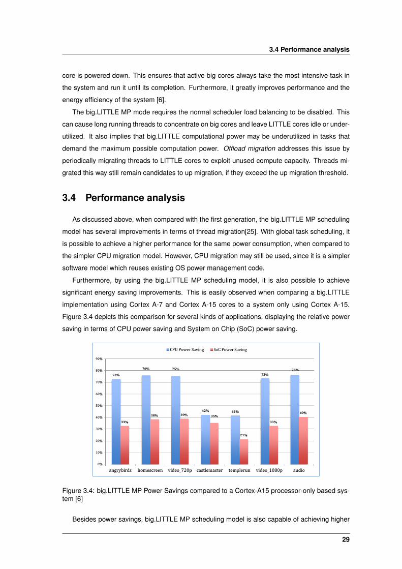
Furthermore, by using the big.LITTLE MP scheduling model, it is also possible to achieve
significant energy saving improvements. This is easily observed when comparing a big.LITTLE
implementation using Cortex A-7 and Cortex A-15 cores to a system only using Cortex A-15.
Figure 3.4 depicts this comparison for several kinds of applications, displaying the relative power
saving in terms of CPU power saving and System on Chip (SoC) power saving.
Figure 3.4: big.LITTLE MP Power Savings compared to a Cortex-A15 processor-only based sys-tem [6]
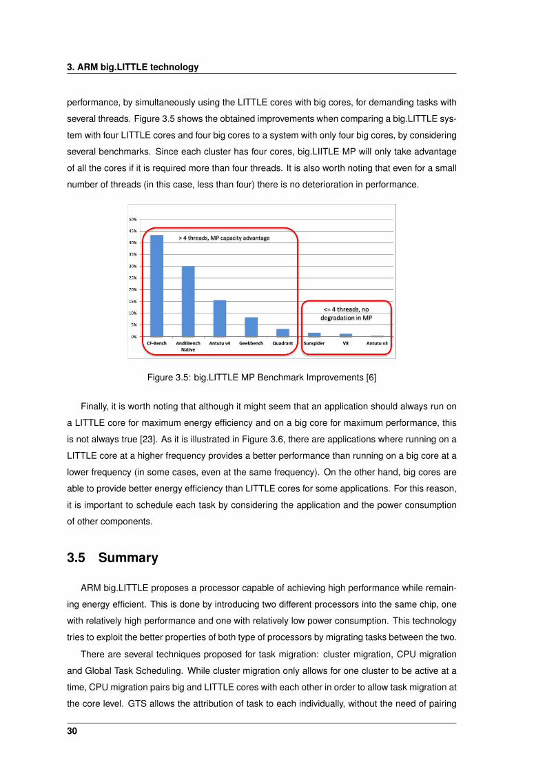
Besides power savings, big.LITTLE MP scheduling model is also capable of achieving higher
29
3. ARM big.LITTLE technology
performance, by simultaneously using the LITTLE cores with big cores, for demanding tasks with
several threads. Figure 3.5 shows the obtained improvements when comparing a big.LITTLE sys-
tem with four LITTLE cores and four big cores to a system with only four big cores, by considering
several benchmarks. Since each cluster has four cores, big.LIITLE MP will only take advantage
of all the cores if it is required more than four threads. It is also worth noting that even for a small
number of threads (in this case, less than four) there is no deterioration in performance.
Figure 3.5: big.LITTLE MP Benchmark Improvements [6]
Finally, it is worth noting that although it might seem that an application should always run on
a LITTLE core for maximum energy efficiency and on a big core for maximum performance, this
is not always true [23]. As it is illustrated in Figure 3.6, there are applications where running on a
LITTLE core at a higher frequency provides a better performance than running on a big core at a
lower frequency (in some cases, even at the same frequency). On the other hand, big cores are
able to provide better energy efficiency than LITTLE cores for some applications. For this reason,
it is important to schedule each task by considering the application and the power consumption
of other components.
3.5 Summary
ARM big.LITTLE proposes a processor capable of achieving high performance while remain-
ing energy efficient. This is done by introducing two different processors into the same chip, one
with relatively high performance and one with relatively low power consumption. This technology
tries to exploit the better properties of both type of processors by migrating tasks between the two.
There are several techniques proposed for task migration: cluster migration, CPU migration
and Global Task Scheduling. While cluster migration only allows for one cluster to be active at a
time, CPU migration pairs big and LITTLE cores with each other in order to allow task migration at
the core level. GTS allows the attribution of task to each individually, without the need of pairing
30

3.5 Summary
(a) Normalized execution time (b) Normalized energy consumption
Figure 3.6: Comparison of execution times and energy efficiency between big and LITTLE cores[23]
cores with each other. This allows for a finer grained task scheduling which provides greater
energy efficiency. In addition, this method allows the utilization of all cores in the processor,
improving overall performance versus the other mentioned methods.
31

3. ARM big.LITTLE technology
32

4State of the art
Contents4.1 Energy efficient HEVC decoding . . . . . . . . . . . . . . . . . . . . . . . . . . 344.2 Proposed approach . . . . . . . . . . . . . . . . . . . . . . . . . . . . . . . . . . 35
33
4. State of the art
In this chapter we will focus in providing context to the development of this work, by presenting
relevant works from other authors. While some of these works may not directly address the exact
same issues as this work, they provide insight into the available technology and possible solutions.
4.1 Energy efficient HEVC decoding
While in this work we focus on video encoding, the decoding process presents similar prob-
lems, such as energy efficiency and performance issues.
Raffin et al. [24] propose a low power HEVC software decoder for mobile devices. Data-level
parallelism and task level parallelism are exploited to reduce the decoding time. A DVFS strategy
adapted to video decoding has been used to improve the energy efficiency compared to existing
DVFS policies. These three optimization strategies were applied to the open source OpenHEVC
decoder and lead to an energy consumption below 21 nano Joules per pixel for HD decoding at
2.2 Mbits/s on a multi-core ARM big.LIITLE processor.
Rodrıguez-Sanchez and Quintana-Ortı [27] present an architecture-aware implementation of
an HEVC decoder on asymmetric multicore processors, more specifically ARM big.LITTLE. The
proposed solution follows the parallelization approach dictated by WPP to distribute the workload
among the big and LITTLE cores in real-time, migrating the threads in charge of executing those
tasks with higher priority to the former type of core. When compared to an implementation which
only exploits the big cores, the exploitation of the Cortex-A7 cores proved to enhance the overall
performance and to improve the energy efficiency of decoding pipeline.
A DVFS based HEVC video decoder implementation is proposed by Nogues et al. [21]. The
typical DVFS execution strategy is called race-to-idle [28], and it tries to execute a task as fast
as possible. This minimizes execution time but at the cost of a high power dissipation during the
execution. However, recent developments on DVFS show that a more energy efficient way of
executing a task is to reduce the CPU frequency to the minimum frequency which still meets the
deadline [13, 15, 16]. For this very reason, the proposed decoder tries to execute the decoding
process as slow as possible while not missing a frame display deadline.
Figure 4.1 show the obtained results for the proposed decoder, for a 720p video decoding
running on a Odroid XU+E, which contains an ARM big.LITTLE processor. The Performance
Linux governor is running at full frequency, while the OnDemand governor is adapting DVFS to
processing load and the presented proposal, PAD, adapts the DVFS to real-time deadlines. The
results show a clear improvement versus the traditional OnDemand governor of Linux, both in
terms of performance and energy efficiency. It also achieves a similar level of energy saving as
a solution previously proposed by the same author, which had tunable image quality as a way to
achieve power savings [22].
He et al. [12] proposed a power aware HEVC system, with the objective of getting the best
34
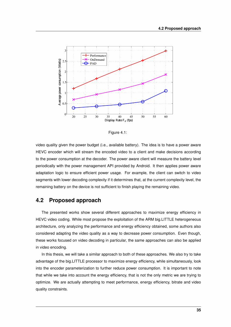
4.2 Proposed approach
Figure 4.1:
video quality given the power budget (i.e., available battery). The idea is to have a power aware
HEVC encoder which will stream the encoded video to a client and make decisions according
to the power consumption at the decoder. The power aware client will measure the battery level
periodically with the power management API provided by Android. It then applies power aware
adaptation logic to ensure efficient power usage. For example, the client can switch to video
segments with lower decoding complexity if it determines that, at the current complexity level, the
remaining battery on the device is not sufficient to finish playing the remaining video.
4.2 Proposed approach
The presented works show several different approaches to maximize energy efficiency in
HEVC video coding. While most propose the exploitation of the ARM big.LITTLE heterogeneous
architecture, only analyzing the performance and energy efficiency obtained, some authors also
considered adapting the video quality as a way to decrease power consumption. Even though,
these works focused on video decoding in particular, the same approaches can also be applied
in video encoding.
In this thesis, we will take a similar approach to both of these approaches. We also try to take
advantage of the big.LITTLE processor to maximize energy efficiency, while simultaneously, look
into the encoder parameterization to further reduce power consumption. It is important to note
that while we take into account the energy efficiency, that is not the only metric we are trying to
optimize. We are actually attempting to meet performance, energy efficiency, bitrate and video
quality constraints.
35

4. State of the art
36

5Energy aware video coding
Contents5.1 Problem formulation . . . . . . . . . . . . . . . . . . . . . . . . . . . . . . . . . 385.2 Proposed solution . . . . . . . . . . . . . . . . . . . . . . . . . . . . . . . . . . . 395.3 Summary . . . . . . . . . . . . . . . . . . . . . . . . . . . . . . . . . . . . . . . . 45
37
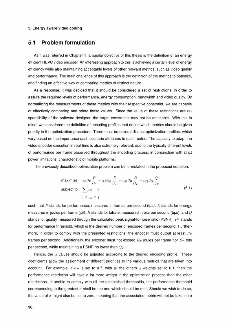
5. Energy aware video coding
5.1 Problem formulation
As it was referred in Chapter 1, a basilar objective of this thesis is the definition of an energy
efficient HEVC video encoder. An interesting approach to this is achieving a certain level of energy
efficiency while also maintaining acceptable levels of other relevant metrics, such as video quality
and performance. The main challenge of this approach is the definition of the metrics to optimize,
and finding an effective way of comparing metrics of distinct nature.
As a response, it was decided that it should be considered a set of restrictions, in order to
assure the required levels of performance, energy consumption, bandwidth and video quality. By
normalizing the measurements of these metrics with their respective constraint, we are capable
of effectively comparing and relate these values. Since the value of these restrictions are re-
sponsibility of the software designer, the target constraints may not be attainable. With this in
mind, we considered the definition of encoding profiles that define which metrics should be given
priority in the optimization procedure. There must be several distinct optimization profiles, which
vary based on the importance each scenario attributes to each metric. The capacity to adapt the
video encoder execution in real-time is also extremely relevant, due to the typically different levels
of performance per frame observed throughout the encoding process, in conjunction with strict
power limitations, characteristic of mobile platforms.
The previously described optimization problem can be formulated in the proposed equation:
maximize αPβPP
PT− αEβE
E
ET− αBβB
B
BT+ αQβQ
Q
QT
subject to∑
αi = 1
0 ≤ αi ≤ 1
(5.1)
such that P stands for performance, measured in frames per second (fps); E stands for energy,
measured in joules per frame (jpf); B stands for bitrate, measured in bits per second (bps); and Q
stands for quality, measured through the calculated peak signal-to-noise ratio (PSNR). PT stands
for performance threshold, which is the desired number of encoded frames per second. Further-
more, in order to comply with the presented restrictions, the encoder must output at least PT
frames per second. Additionally, the encoder must not exceed ET joules per frame nor BT bits
per second, while maintaining a PSNR no lower than QT .
Hence, the α values should be adjusted according to the desired encoding profile. These
coefficients allow the assignment of different priorities to the various metrics that are taken into
account. For example, if αP is set to 0.7, with all the others α weights set to 0.1, then the
performance restriction will have a lot more weight in the optimization process than the other
restrictions. If unable to comply with all the established thresholds, the performance threshold
corresponding to the greatest α shall be the one which should be met. Should we wish to do so,
the value of α might also be set to zero, meaning that the associated metric will not be taken into
38
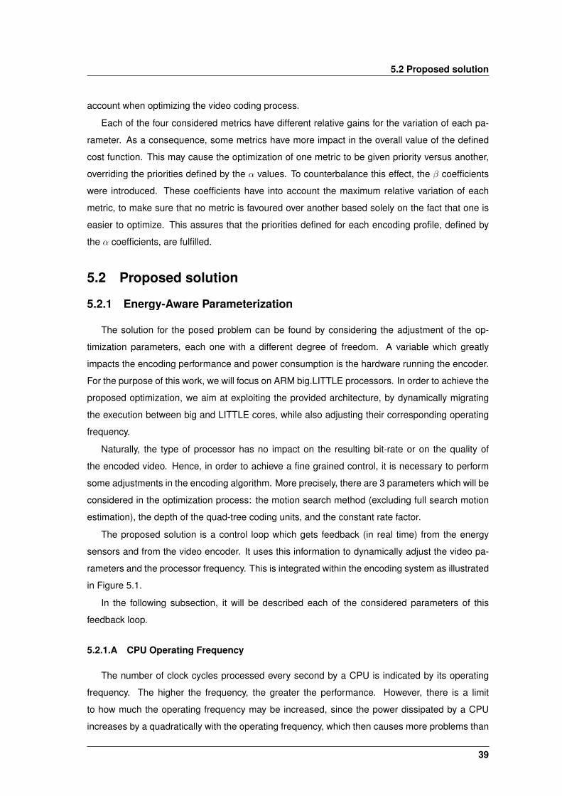
5.2 Proposed solution
account when optimizing the video coding process.
Each of the four considered metrics have different relative gains for the variation of each pa-
rameter. As a consequence, some metrics have more impact in the overall value of the defined
cost function. This may cause the optimization of one metric to be given priority versus another,
overriding the priorities defined by the α values. To counterbalance this effect, the β coefficients
were introduced. These coefficients have into account the maximum relative variation of each
metric, to make sure that no metric is favoured over another based solely on the fact that one is
easier to optimize. This assures that the priorities defined for each encoding profile, defined by
the α coefficients, are fulfilled.
5.2 Proposed solution
5.2.1 Energy-Aware Parameterization
The solution for the posed problem can be found by considering the adjustment of the op-
timization parameters, each one with a different degree of freedom. A variable which greatly
impacts the encoding performance and power consumption is the hardware running the encoder.
For the purpose of this work, we will focus on ARM big.LITTLE processors. In order to achieve the
proposed optimization, we aim at exploiting the provided architecture, by dynamically migrating
the execution between big and LITTLE cores, while also adjusting their corresponding operating
frequency.
Naturally, the type of processor has no impact on the resulting bit-rate or on the quality of
the encoded video. Hence, in order to achieve a fine grained control, it is necessary to perform
some adjustments in the encoding algorithm. More precisely, there are 3 parameters which will be
considered in the optimization process: the motion search method (excluding full search motion
estimation), the depth of the quad-tree coding units, and the constant rate factor.
The proposed solution is a control loop which gets feedback (in real time) from the energy
sensors and from the video encoder. It uses this information to dynamically adjust the video pa-
rameters and the processor frequency. This is integrated within the encoding system as illustrated
in Figure 5.1.
In the following subsection, it will be described each of the considered parameters of this
feedback loop.
5.2.1.A CPU Operating Frequency
The number of clock cycles processed every second by a CPU is indicated by its operating
frequency. The higher the frequency, the greater the performance. However, there is a limit
to how much the operating frequency may be increased, since the power dissipated by a CPU
increases by a quadratically with the operating frequency, which then causes more problems than
39
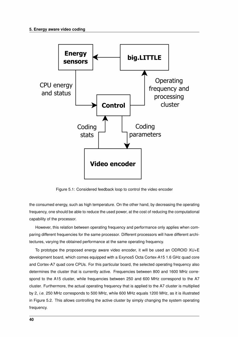
5. Energy aware video coding
Figure 5.1: Considered feedback loop to control the video encoder
the consumed energy, such as high temperature. On the other hand, by decreasing the operating
frequency, one should be able to reduce the used power, at the cost of reducing the computational
capability of the processor.
However, this relation between operating frequency and performance only applies when com-
paring different frequencies for the same processor. Different processors will have different archi-
tectures, varying the obtained performance at the same operating frequency.
To prototype the proposed energy aware video encoder, it will be used an ODROID XU+E
development board, which comes equipped with a Exynos5 Octa Cortex-A15 1.6 GHz quad core
and Cortex-A7 quad core CPUs. For this particular board, the selected operating frequency also
determines the cluster that is currently active. Frequencies between 800 and 1600 MHz corre-
spond to the A15 cluster, while frequencies between 250 and 600 MHz correspond to the A7
cluster. Furthermore, the actual operating frequency that is applied to the A7 cluster is multiplied
by 2, i.e. 250 MHz corresponds to 500 MHz, while 600 MHz equals 1200 MHz, as it is illustrated
in Figure 5.2. This allows controlling the active cluster by simply changing the system operating
frequency.
40
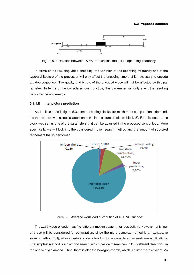
5.2 Proposed solution
Figure 5.2: Relation between DVFS frequencies and actual operating frequency
In terms of the resulting video encoding, the variation of the operating frequency and of the
type/architecture of the processor will only affect the encoding time that is necessary to encode
a video sequence. The quality and bitrate of the encoded video will not be affected by this pa-
rameter. In terms of the considered cost function, this parameter will only affect the resulting
performance and energy.
5.2.1.B Inter picture prediction
As it is illustrated in figure 5.3, some encoding blocks are much more computational demand-
ing than others, with a special attention to the inter picture prediction block [5]. For this reason, this
block was set as one of the parameters that can be adjusted in the proposed control loop. More
specifically, we will look into the considered motion search method and the amount of sub-pixel
refinement that is performed.
Figure 5.3: Average work load distribution of a HEVC encoder
The x265 video encoder has five different motion search methods built in. However, only four
of these will be considered for optimization, since the more complex method is an exhaustive
search method (full), whose performance is too low to be considered for real-time applications.
The simplest method is a diamond search, which basically searches in four different directions, in
the shape of a diamond. Then, there is also the hexagon search, which is a little more efficient. As
41
5. Energy aware video coding
more complex methods, there is the Uneven Multi-Hexagon (UMH) search, which is an adaption
of the search method used by x264 for slower presets. Finally, there is also the denominated
star method, which is a three step search adapted from the HM encoder: a star-pattern search
followed by an optional radix scan, followed by an optional star-search refinement [19].
The sub-pixel refinement block controls how much time and effort the encoder should put into
CU partitioning decisions and final motion-vector refinement for quarter-pixel motion vectors. A
more thorough evaluation of the motion vectors will find better matches, producing better motion
vectors, and leading to a less complex residual image left to encode after motion compensation,
therefore providing a better quality at the given target bitrate. Naturally, a more thorough evalua-
tion will be more computationally demanding.
Overall, these parameters have a high impact on the video encoder performance and on
amount energy that is spent, while having relatively less impact on the resulting bitrate and quality
of the encoded video.
5.2.1.C Coding Tree Unit Depth
As it was referred in section 2.1.2, a video encoder compliant with the HEVC standard will
start the encoding procedure of each frame by dividing it into smaller blocks, called Coding Tree
Units (CTUs). Each of these CTUs has a size of 64 by 64 pixels, and may then be subdivided into
four smaller blocks of 32 by 32 pixels, and each of these blocks may be then further subdivided
into four smaller blocks, up to blocks of 8 by 8 pixels. This subdivision is usually done based on
the redundancy level in the considered CTU, i.e. for more detailed blocks the subdivision will be
higher, while for relatively less detailed blocks there will be little or no division into smaller blocks.
Hence, the CTU depth refers to how many times is the encoder allowed to subdivide each
CTU, up to a minimum block size of 8 by 8 pixels. A higher CTU depth will be reflected in an
higher video quality and lower bitrate. However, this also means a relatively lower performance
and higher energy usage.
5.2.1.D Constant Rate Factor
The Constant Rate Factor (CRF) is a method of quality control that tries to achieve an uniform
video quality in the encoded video sequence. A typical video sequence has frames of high move-
ment and of little to no movement, with the high movement frames being more difficult to encode
due to lower pixel redundancy. In order to achieved an uniform video quality throughout the whole
video sequence, the bitrate must compensate the video frames of higher movement. This means
that scenes with more movement will see an increase in bitrate.
The embedded rate controller causes the mentioned increase in the bitrate, by making ad-
justments to the quantization step according to how much the encoded frames deviate from the
specified rate factor. The lower the rate factor, the better the quality of the encoded video, but the
42
5.2 Proposed solution
higher the bitrate. If the rate factor is too low, then the produced sequence will have a very low
compression ratio. If it is too high, the quality of the video will be too low, making it incomprehen-
sible. For this reason, only values between 24 and 34 will be considered when performing online
adaptations to the rate factor.
In accordance, varying the rate factor has a great impact on the resulting video quality and
bitrate, but it also reflected on the encoding performance and the used energy. By increasing the
rate factor, it will result in a higher encoding performance, as well as a better energy efficiency
and lower bitrate, at the cost of a lower video quality.
5.2.2 Optimization Algorithm
As it was previously mentioned, in order to achieve a video encoder which complies with
specific restrictions in terms of the resulting bitrate, quality, performance and energy levels, it was
embedded a new controller in the video encoder that adapts the configuration of the CPU and the
parameters of the encoder in real time. We will now focus in the way the control loop achieves
this, by explaining the implemented optimization algorithm, which is illustrated in Figure 5.4
The first step to optimize the execution of our video encoder is to determine where it stands and
how it relates to the restrictions in place. We will refer to this as the functional point of our video
encoder. The first few encoded frames are spent by collecting relevant data, in order to determine
this functional point. This causes the introduction of some latency in the control loop, since only
after the mentioned first few frames, will it actually start optimizing the video encoder. However,
this latency is necessary, since the very first encoded video frames are not representative of the
video encoder normal execution, mainly due to the lack of long-term redundancy in these frames.
If we would not wait these few frames, our control loop would start optimizing the encoder right
away, but with a very high risk of adapting the functional point towards a wrong direction or by an
excessive amount, which would ultimately not benefit our optimization purpose in any way.
Having determined the functional point, the algorithm proceeds with the determination of the
parameters that have to be changed, in order to maximize the cost function. For such purpose,
the algorithm analyses each of the previously mentioned encoding parameters and computes, for
each one, the optimal value of that parameter, i.e. the value which maximizes the cost function.
However, since each parameter is individually analysed, it must assure that the combination of all
parameters still corresponds to the optimal functional point. In the cases it does not, the algorithm
will try all possible combinations of parameters until it finds the combination that achieves the best
(non-optimal) value for the cost function.
The conducted adjustments to the encoder parameters are based on a previously determined
variation role. This role is empirically obtained, which means that it may not reflect the actual gains
obtained for the current video, since the obtained gain tends to vary with the type of video. Unless
To compensate for this fact, we dynamically adjust these roles according to the gains obtained
43
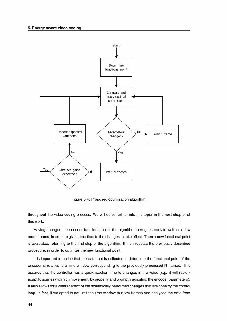
5. Energy aware video coding
Figure 5.4: Proposed optimization algorithm.
throughout the video coding process. We will delve further into this topic, in the next chapter of
this work.
Having changed the encoder functional point, the algorithm then goes back to wait for a few
more frames, in order to give some time to the changes to take effect. Then a new functional point
is evaluated, returning to the first step of the algorithm. It then repeats the previously described
procedure, in order to optimize the new functional point.
It is important to notice that the data that is collected to determine the functional point of the
encoder is relative to a time window corresponding to the previously processed N frames. This
assures that the controller has a quick reaction time to changes in the video (e.g. it will rapidly
adapt to scenes with high movement, by properly and promptly adjusting the encoder parameters).
It also allows for a clearer effect of the dynamically performed changes that are done by the control
loop. In fact, If we opted to not limit the time window to a few frames and analysed the data from
44
5.3 Summary
the start of the encoding process to the current frame, then the functional point would be heavily
influenced by all the frames preceding the current one. To exemplify, let us assume we performed
an adjustment to the parameters based on a N=300 time window and waited 10 more frames to
give time for the change to take effect. By analysing the data since the start of the video, we would
have 300 frames with the parameters before the change and only 10 frames after the change. The
functional point of these 310 frames would differ a lot from the obtained one before the first 300
frames, even if it was a radical change. However, if we limit our window to the previous 10 frames,
we will have a very clear picture of how our changes affected the functional point.
5.3 Summary
In order to achieve an energy efficient HEVC encoder, a controller is introduced. The controller
receives information about each encoded frame, analyzing the performance, energy efficiency,
bitrate and video quality. Based on this information, it will then adjust the encoder parameters and
CPU frequency, in order to meet several restraints of the previously mentioned metrics.
The controller basis its optimization decisions in predetermined values respective to the ex-
pected variation of each of the considered optimization parameters. In order for the optimization
algorithm to dynamically adapt to variations in the video sequence, the expected variation values
are updated during the encoding procedure.
Additionally, the proposed optimization algorithm defines several optimization profiles, which
establish priorities between the metrics to optimize.
45

5. Energy aware video coding
46
6Implementation of the proposed
encoder modification
Contents6.1 Encoder Sensing . . . . . . . . . . . . . . . . . . . . . . . . . . . . . . . . . . . 486.2 Encoder Parameterization . . . . . . . . . . . . . . . . . . . . . . . . . . . . . . 506.3 Cost Function Parameterization . . . . . . . . . . . . . . . . . . . . . . . . . . . 546.4 Summary . . . . . . . . . . . . . . . . . . . . . . . . . . . . . . . . . . . . . . . . 56
47
6. Implementation of the proposed encoder modification
6.1 Encoder Sensing
One crucial aspect of the proposed control algorithm (see 5.2.2), is the determination of the
encoder’s functional point. This is achieved by extracting and analyzing statistics relative to the
encoder execution. This section will describe the methods used to obtain and process this data
in real-time.
6.1.1 Encoding Statistics
In the previous chapter, the envisaged optimization approach of the video encoder was dis-
cussed, based on four distinct metrics: performance, energy, bitrate and quality. These metrics
are measured in frames per second, Joules per frame, bits per second and Peak Signal to Noise
Ratio (PSNR), respectively. This information is extracted from the encoder at the end of every
encoded frame.
In particular, the considered HEVC encoder implementation (x265), has a built in function
which allows to extract the main statistics of the current execution, denominated as x265 encoder
get stats(). Among these statistics are the referred metrics for performance, bitrate and quality.
However, the obtained values are measured from the start of the encoding procedure until the
current frame. Since we want to analyse these metrics only at the past few frames, to assure
a more dynamic control loop, we can not directly extract those statistics by directly using this
method. Nevertheless, we are still able to use this built-in feature at a cost of some manipulations
in order to obtain the information we want.
The encoding performance metric (frames per second) is the most straightforward metric to ex-
tract. We simply measure how much time is elapsed in the encoding of each frame. By dividing the
number of considered frames by the sum of the elapsed processing time of each frame we obtain
the required performance metric. For the birate and energy metric the procedure is not as straight-
forward but still quite simple. With the aid of previously mentioned x265 encoder get stats(),
we are able to extract the total bits encoded since the start, as well as the sum of the PSNR of
each encoded frame. To convert these values to the required metrics that only consider a limited
number of frames, we simply subtract the value extracted at the frame we want as our first frame
to the value obtained for the current frame. Then, we only have to divide by the total elapsed time
for the considered frames to obtain the bits per second, our bitrate metric. For the quality metric,
we do a similar procedure that takes the difference between the measured PSNR value at the first
and last considered frames and divides it by the number of considered frames.
In order to measure the amount of energy that is spent in the encoding process, we will take
advantage of the energy sensors provided to measure the power usage of our CPU. Only the
CPU is considered because this is the only component which will directly be affected by the
implement control loop. We are able to individually measure the energy of each of the CPU
48
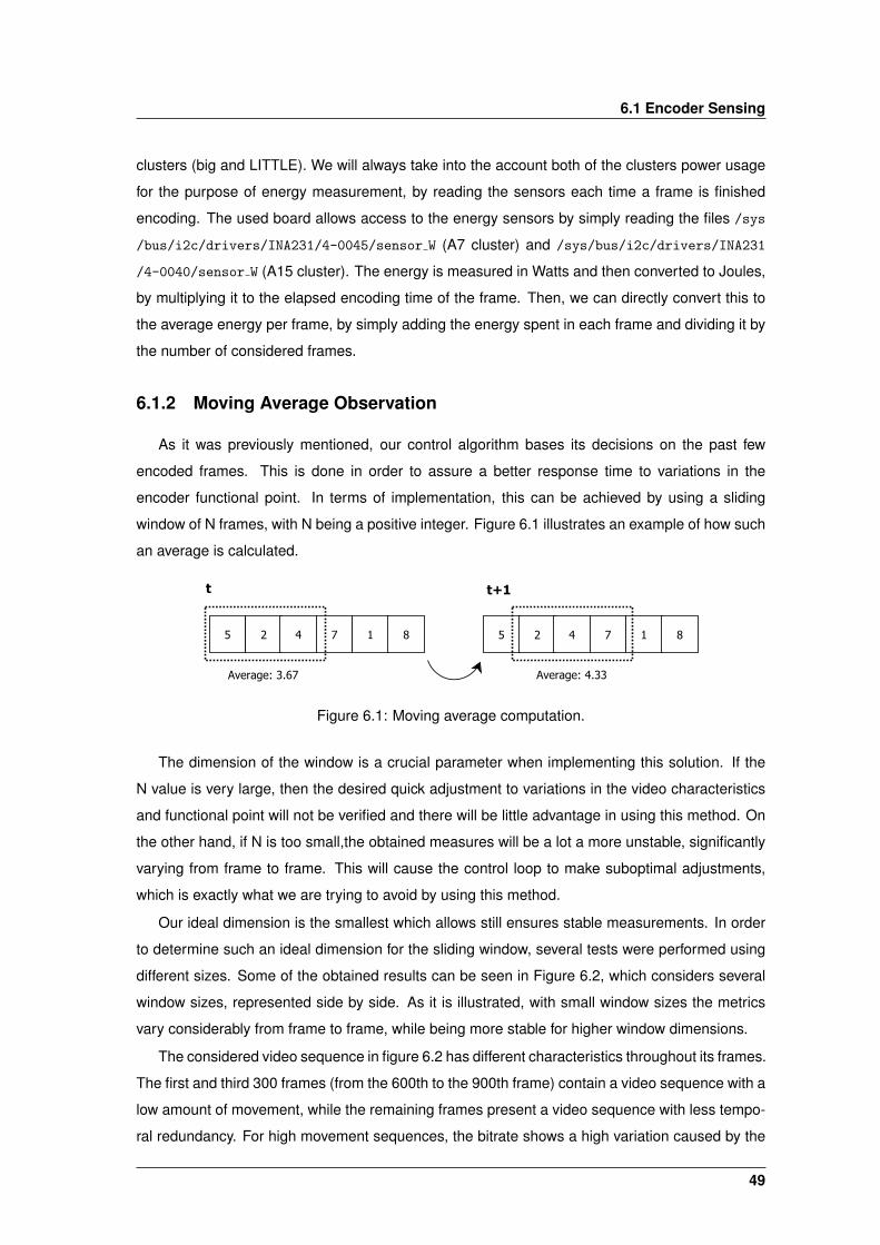
6.1 Encoder Sensing
clusters (big and LITTLE). We will always take into the account both of the clusters power usage
for the purpose of energy measurement, by reading the sensors each time a frame is finished
encoding. The used board allows access to the energy sensors by simply reading the files /sys
/bus/i2c/drivers/INA231/4-0045/sensor W (A7 cluster) and /sys/bus/i2c/drivers/INA231
/4-0040/sensor W (A15 cluster). The energy is measured in Watts and then converted to Joules,
by multiplying it to the elapsed encoding time of the frame. Then, we can directly convert this to
the average energy per frame, by simply adding the energy spent in each frame and dividing it by
the number of considered frames.
6.1.2 Moving Average Observation
As it was previously mentioned, our control algorithm bases its decisions on the past few
encoded frames. This is done in order to assure a better response time to variations in the
encoder functional point. In terms of implementation, this can be achieved by using a sliding
window of N frames, with N being a positive integer. Figure 6.1 illustrates an example of how such
an average is calculated.
Figure 6.1: Moving average computation.
The dimension of the window is a crucial parameter when implementing this solution. If the
N value is very large, then the desired quick adjustment to variations in the video characteristics
and functional point will not be verified and there will be little advantage in using this method. On
the other hand, if N is too small,the obtained measures will be a lot a more unstable, significantly
varying from frame to frame. This will cause the control loop to make suboptimal adjustments,
which is exactly what we are trying to avoid by using this method.
Our ideal dimension is the smallest which allows still ensures stable measurements. In order
to determine such an ideal dimension for the sliding window, several tests were performed using
different sizes. Some of the obtained results can be seen in Figure 6.2, which considers several
window sizes, represented side by side. As it is illustrated, with small window sizes the metrics
vary considerably from frame to frame, while being more stable for higher window dimensions.
The considered video sequence in figure 6.2 has different characteristics throughout its frames.
The first and third 300 frames (from the 600th to the 900th frame) contain a video sequence with a
low amount of movement, while the remaining frames present a video sequence with less tempo-
ral redundancy. For high movement sequences, the bitrate shows a high variation caused by the
49
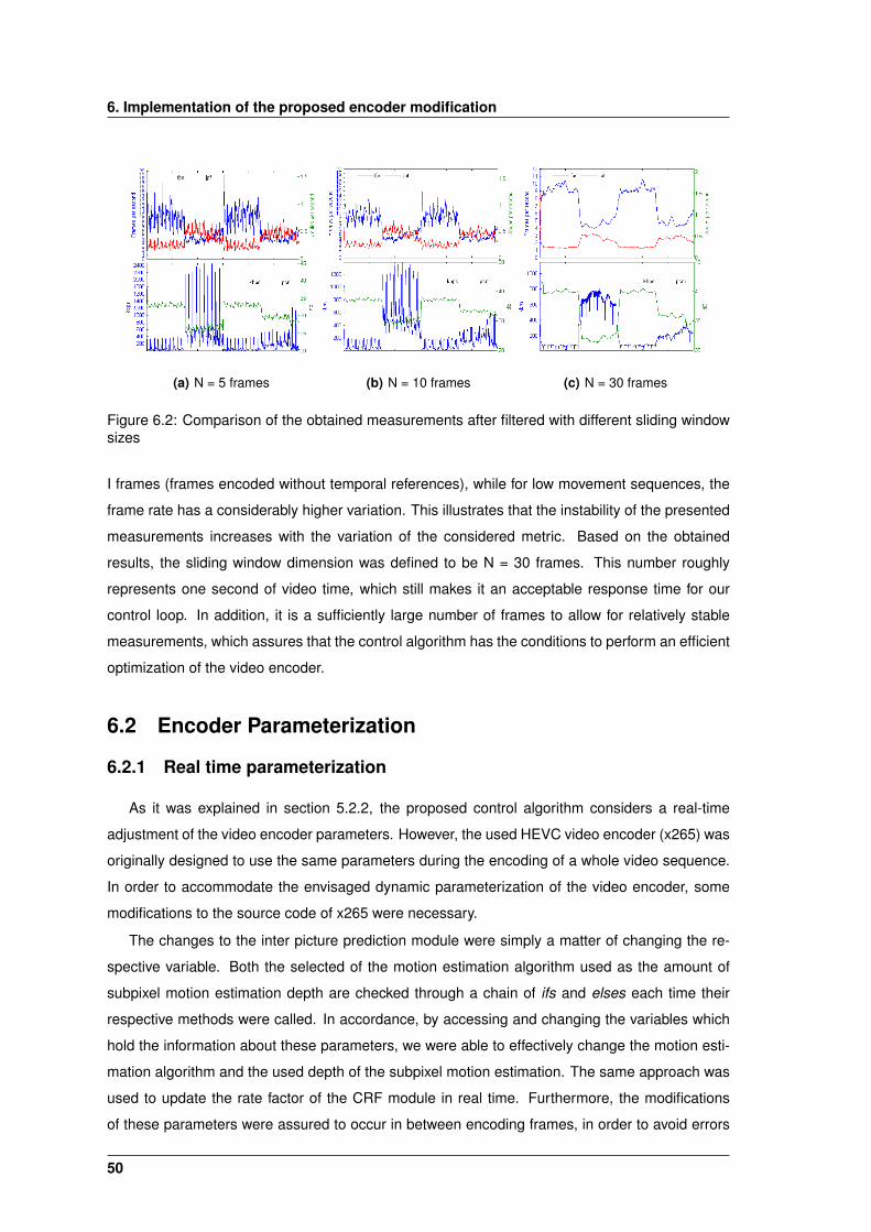
6. Implementation of the proposed encoder modification
(a) N = 5 frames (b) N = 10 frames (c) N = 30 frames
Figure 6.2: Comparison of the obtained measurements after filtered with different sliding windowsizes
I frames (frames encoded without temporal references), while for low movement sequences, the
frame rate has a considerably higher variation. This illustrates that the instability of the presented
measurements increases with the variation of the considered metric. Based on the obtained
results, the sliding window dimension was defined to be N = 30 frames. This number roughly
represents one second of video time, which still makes it an acceptable response time for our
control loop. In addition, it is a sufficiently large number of frames to allow for relatively stable
measurements, which assures that the control algorithm has the conditions to perform an efficient
optimization of the video encoder.
6.2 Encoder Parameterization
6.2.1 Real time parameterization
As it was explained in section 5.2.2, the proposed control algorithm considers a real-time
adjustment of the video encoder parameters. However, the used HEVC video encoder (x265) was
originally designed to use the same parameters during the encoding of a whole video sequence.
In order to accommodate the envisaged dynamic parameterization of the video encoder, some
modifications to the source code of x265 were necessary.
The changes to the inter picture prediction module were simply a matter of changing the re-
spective variable. Both the selected of the motion estimation algorithm used as the amount of
subpixel motion estimation depth are checked through a chain of ifs and elses each time their
respective methods were called. In accordance, by accessing and changing the variables which
hold the information about these parameters, we were able to effectively change the motion esti-
mation algorithm and the used depth of the subpixel motion estimation. The same approach was
used to update the rate factor of the CRF module in real time. Furthermore, the modifications
of these parameters were assured to occur in between encoding frames, in order to avoid errors
50
6.2 Encoder Parameterization
which might occur by changing this configurations in the middle of the encoding of a given frame.
Nevertheless, changing the parameterization corresponding to the CTU depth in real-time
proved to be a more delicate endeavor. In fact, the encoder expects to use the same CTU max
depth for all the frames of the same GOP. As a consequence, if we force the modification of the
CTU depth parameter to a deeper value, then the program aborts due to trying to access an
invalid memory position. In fact, since the encoder expects a certain depth along its encoding, it
will go beyond the modified CTU depth, since it basis its decision on the CTU max depth value
that was defined for that specific GOP. This problem does not happen when increasing the max
CTU depth since then the program will not try to go beyond the established depth, but it will also
not benefit from the extended CTU depth. Hence, only at the start of a new GOP will the changes
of the CTU max depth take into effect, so the controller waits for the end of the current GOP before
the applying changes to the CTU max depth.
In terms of source code, the mentioned modifications were reflected in the x265 encoder
class, which defines the video encoder. This contains a structure, x265 param, that holds most
of the encoder configurations, such as motion estimation algorithm (searchMethod), used depth
of the subpixel motion estimation (subpelRefine) and CTU depth (minCUSize). However, this
structure does not contain information relative to the rate control, to adjust that parameter another
class (RateControl) must be accessed. The x265 encoder contains a pointer to RateControl
(m rateControl) which enables the alteration of the CRF rate factor by changing m rateControl
->m rateFactorConstant. By modifying these variables as previously explained, we are able to
change the encoder parameters during its execution.
In addition to the encoder parameters, the controller also adjusts the CPU operating frequency
and active cluster. As explained in the previous chapter (see 5.2.1.A), the active cluster is implic-
itly changed by changing the operating frequency. While operating at values between 250 MHz
and 600 Mhz, the LITTLE cluster will be active. Operating at values between 800 and 1600 MHz
results in the big cluster to be active. The used operating system (Linux 3.4.84) allowed the ad-
justment of the operating frequency by changing the scaling governor and scaling setspeed,
accessible through the directory /sys/devices/system/cpu/cpu0/cpufreq. The scaling gover-
nor must be set to ”userspace” for the frequencies set through scaling setspeed to be applied.
6.2.2 Expected variation
As it was explained in the previous chapter, the proposed control algorithm makes its decisions
based on the expected variation for each of the considered parameters. While the direction in
which it is necessary to vary each parameter is easy to determine, the same is not true in what
concerns the amount of variation. In fact, by having the additional information about the expected
variation that a certain adjustment of the encoder considered parameter will have in the encoder
functional point, we are able to vary the parameter only by the required amount that is necessary
51
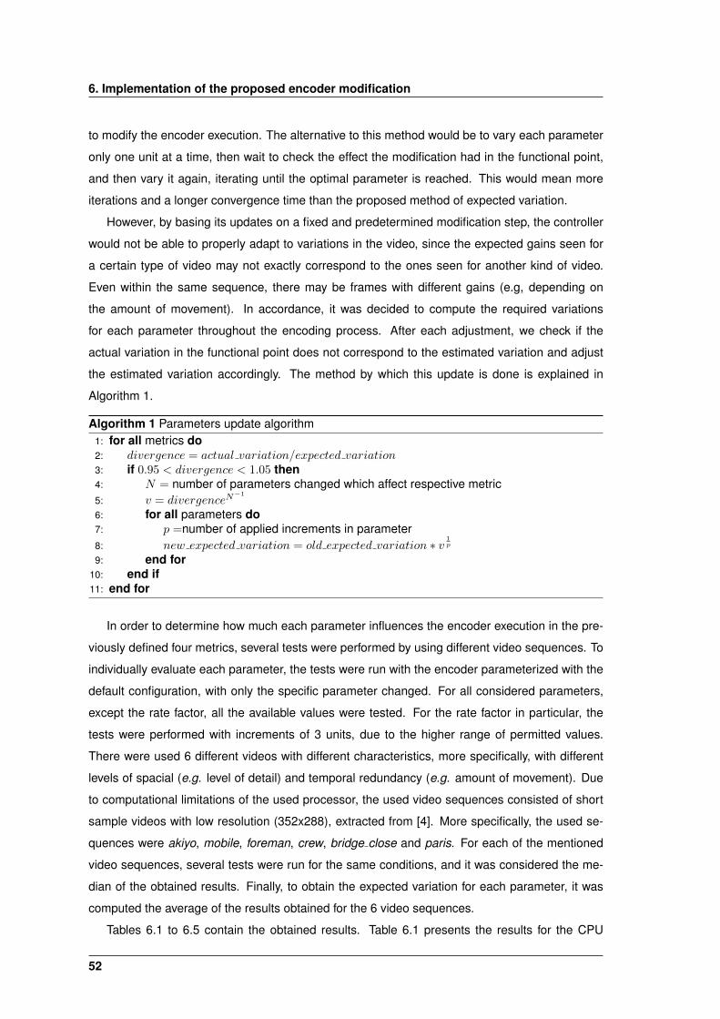
6. Implementation of the proposed encoder modification
to modify the encoder execution. The alternative to this method would be to vary each parameter
only one unit at a time, then wait to check the effect the modification had in the functional point,
and then vary it again, iterating until the optimal parameter is reached. This would mean more
iterations and a longer convergence time than the proposed method of expected variation.
However, by basing its updates on a fixed and predetermined modification step, the controller
would not be able to properly adapt to variations in the video, since the expected gains seen for
a certain type of video may not exactly correspond to the ones seen for another kind of video.
Even within the same sequence, there may be frames with different gains (e.g, depending on
the amount of movement). In accordance, it was decided to compute the required variations
for each parameter throughout the encoding process. After each adjustment, we check if the
actual variation in the functional point does not correspond to the estimated variation and adjust
the estimated variation accordingly. The method by which this update is done is explained in
Algorithm 1.
Algorithm 1 Parameters update algorithm1: for all metrics do2: divergence = actual variation/expected variation3: if 0.95 < divergence < 1.05 then4: N = number of parameters changed which affect respective metric5: v = divergenceN
−1
6: for all parameters do7: p =number of applied increments in parameter8: new expected variation = old expected variation ∗ v
1p
9: end for10: end if11: end for
In order to determine how much each parameter influences the encoder execution in the pre-
viously defined four metrics, several tests were performed by using different video sequences. To
individually evaluate each parameter, the tests were run with the encoder parameterized with the
default configuration, with only the specific parameter changed. For all considered parameters,
except the rate factor, all the available values were tested. For the rate factor in particular, the
tests were performed with increments of 3 units, due to the higher range of permitted values.
There were used 6 different videos with different characteristics, more specifically, with different
levels of spacial (e.g. level of detail) and temporal redundancy (e.g. amount of movement). Due
to computational limitations of the used processor, the used video sequences consisted of short
sample videos with low resolution (352x288), extracted from [4]. More specifically, the used se-
quences were akiyo, mobile, foreman, crew, bridge close and paris. For each of the mentioned
video sequences, several tests were run for the same conditions, and it was considered the me-
dian of the obtained results. Finally, to obtain the expected variation for each parameter, it was
computed the average of the results obtained for the 6 video sequences.
Tables 6.1 to 6.5 contain the obtained results. Table 6.1 presents the results for the CPU
52
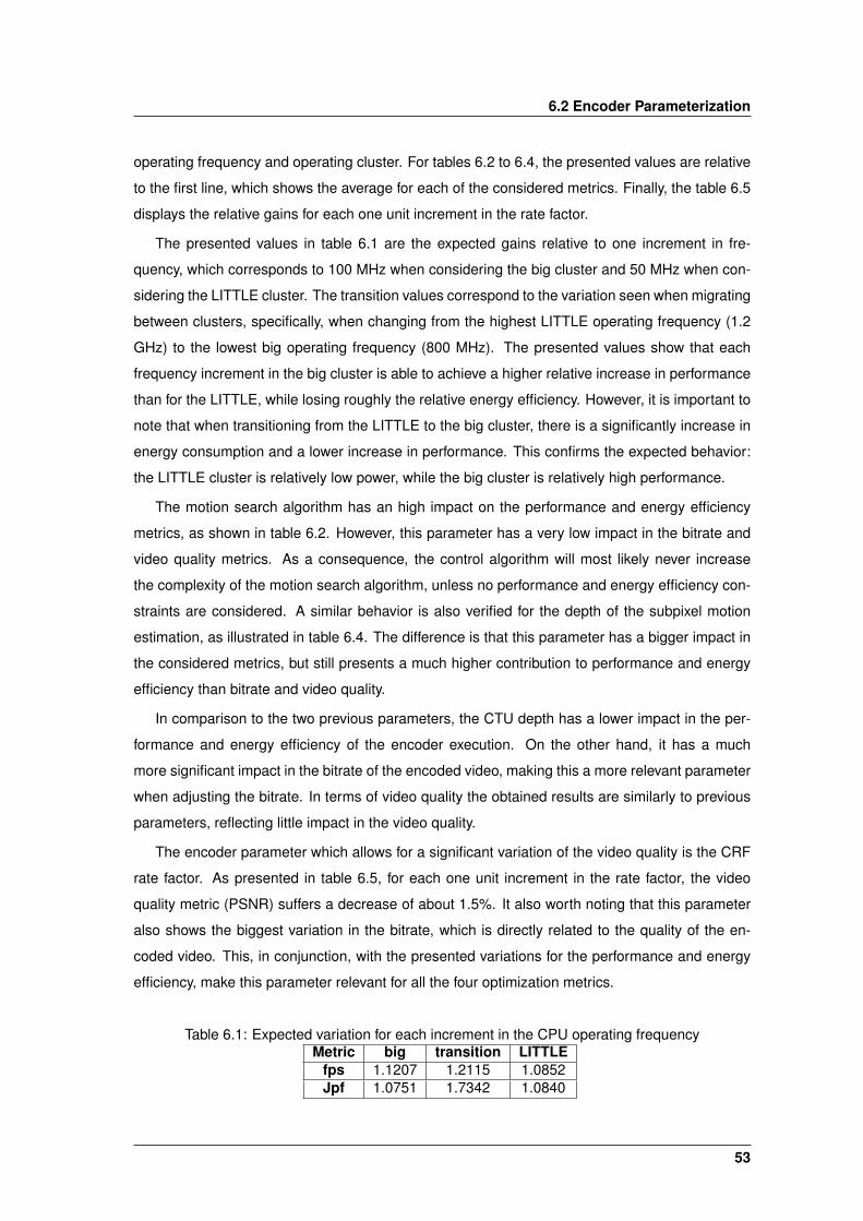
6.2 Encoder Parameterization
operating frequency and operating cluster. For tables 6.2 to 6.4, the presented values are relative
to the first line, which shows the average for each of the considered metrics. Finally, the table 6.5
displays the relative gains for each one unit increment in the rate factor.
The presented values in table 6.1 are the expected gains relative to one increment in fre-
quency, which corresponds to 100 MHz when considering the big cluster and 50 MHz when con-
sidering the LITTLE cluster. The transition values correspond to the variation seen when migrating
between clusters, specifically, when changing from the highest LITTLE operating frequency (1.2
GHz) to the lowest big operating frequency (800 MHz). The presented values show that each
frequency increment in the big cluster is able to achieve a higher relative increase in performance
than for the LITTLE, while losing roughly the relative energy efficiency. However, it is important to
note that when transitioning from the LITTLE to the big cluster, there is a significantly increase in
energy consumption and a lower increase in performance. This confirms the expected behavior:
the LITTLE cluster is relatively low power, while the big cluster is relatively high performance.
The motion search algorithm has an high impact on the performance and energy efficiency
metrics, as shown in table 6.2. However, this parameter has a very low impact in the bitrate and
video quality metrics. As a consequence, the control algorithm will most likely never increase
the complexity of the motion search algorithm, unless no performance and energy efficiency con-
straints are considered. A similar behavior is also verified for the depth of the subpixel motion
estimation, as illustrated in table 6.4. The difference is that this parameter has a bigger impact in
the considered metrics, but still presents a much higher contribution to performance and energy
efficiency than bitrate and video quality.
In comparison to the two previous parameters, the CTU depth has a lower impact in the per-
formance and energy efficiency of the encoder execution. On the other hand, it has a much
more significant impact in the bitrate of the encoded video, making this a more relevant parameter
when adjusting the bitrate. In terms of video quality the obtained results are similarly to previous
parameters, reflecting little impact in the video quality.
The encoder parameter which allows for a significant variation of the video quality is the CRF
rate factor. As presented in table 6.5, for each one unit increment in the rate factor, the video
quality metric (PSNR) suffers a decrease of about 1.5%. It also worth noting that this parameter
also shows the biggest variation in the bitrate, which is directly related to the quality of the en-
coded video. This, in conjunction, with the presented variations for the performance and energy
efficiency, make this parameter relevant for all the four optimization metrics.
Table 6.1: Expected variation for each increment in the CPU operating frequencyMetric big transition LITTLE
fps 1.1207 1.2115 1.0852Jpf 1.0751 1.7342 1.0840
53
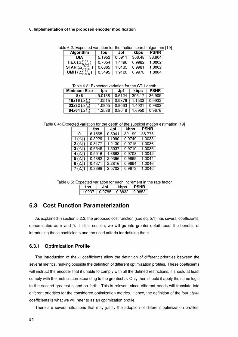
6. Implementation of the proposed encoder modification
Table 6.2: Expected variation for the motion search algorithm [19]Algorithm fps Jpf kbps PSNR
DIA 5.1952 0.5911 306.48 36.904HEX (∆DIA
HEX ) 0.7654 1.4496 0.9982 1.0002STAR (∆DIA
STAR) 0.6865 1.6135 0.9981 1.0002UMH (∆DIA
UMH ) 0.5495 1.9120 0.9978 1.0004
Table 6.3: Expected variation for the CTU depthMinimum Size fps Jpf kbps PSNR
8x8 5.0188 0.6124 306.17 36.90516x16 (∆8
16) 1.0515 0.9376 1.1533 0.993232x32 (∆8
32) 1.0905 0.9063 1.4021 0.980264x64 (∆8
64) 1.3586 0.8048 1.6950 0.9676
Table 6.4: Expected variation for the depth of the subpixel motion estimation [19]fps Jpf kbps PSNR
0 6.1565 0.5041 321.99 36.7751 (∆0
1) 0.8229 1.1990 0.9749 1.00332 (∆0
2) 0.8177 1.2130 0.9715 1.00363 (∆0
3) 0.6545 1.5037 0.9710 1.00364 (∆0
4) 0.5916 1.6663 0.9708 1.00425 (∆0
5) 0.4882 2.0396 0.9699 1.00446 (∆0
6) 0.4371 2.2816 0.9694 1.00467 (∆0
7) 0.3898 2.5702 0.9673 1.0046
Table 6.5: Expected variation for each increment in the rate factorfps Jpf kbps PSNR
1.0237 0.9785 0.8832 0.9853
6.3 Cost Function Parameterization
As explained in section 5.2.2, the proposed cost function (see eq. 5.1) has several coefficients,
denominated as α and β. In this section, we will go into greater detail about the benefits of
introducing these coefficients and the used criteria for defining them.
6.3.1 Optimization Profile
The introduction of the α coefficients allow the definition of different priorities between the
several metrics, making possible the definition of different optimization profiles. These coefficients
will instruct the encoder that if unable to comply with all the defined restrictions, it should at least
comply with the metrics corresponding to the greatest α. Only then should it apply the same logic
to the second greatest α and so forth. This is relevant since different needs will translate into
different priorities for the considered optimization metrics. Hence, the definition of the four alpha
coefficients is what we will refer to as an optimization profile.
There are several situations that may justify the adoption of different optimization profiles.
54
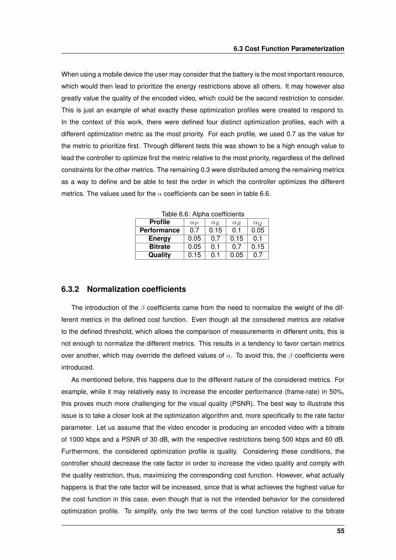
6.3 Cost Function Parameterization
When using a mobile device the user may consider that the battery is the most important resource,
which would then lead to prioritize the energy restrictions above all others. It may however also
greatly value the quality of the encoded video, which could be the second restriction to consider.
This is just an example of what exactly these optimization profiles were created to respond to.
In the context of this work, there were defined four distinct optimization profiles, each with a
different optimization metric as the most priority. For each profile, we used 0.7 as the value for
the metric to prioritize first. Through different tests this was shown to be a high enough value to
lead the controller to optimize first the metric relative to the most priority, regardless of the defined
constraints for the other metrics. The remaining 0.3 were distributed among the remaining metrics
as a way to define and be able to test the order in which the controller optimizes the different
metrics. The values used for the α coefficients can be seen in table 6.6.
Table 6.6: Alpha coefficientsProfile αP αE αB αQ
Performance 0.7 0.15 0.1 0.05Energy 0.05 0.7 0.15 0.1Bitrate 0.05 0.1 0.7 0.15Quality 0.15 0.1 0.05 0.7
6.3.2 Normalization coefficients
The introduction of the β coefficients came from the need to normalize the weight of the dif-
ferent metrics in the defined cost function. Even though all the considered metrics are relative
to the defined threshold, which allows the comparison of measurements in different units, this is
not enough to normalize the different metrics. This results in a tendency to favor certain metrics
over another, which may override the defined values of α. To avoid this, the β coefficients were
introduced.
As mentioned before, this happens due to the different nature of the considered metrics. For
example, while it may relatively easy to increase the encoder performance (frame-rate) in 50%,
this proves much more challenging for the visual quality (PSNR). The best way to illustrate this
issue is to take a closer look at the optimization algorithm and, more specifically to the rate factor
parameter. Let us assume that the video encoder is producing an encoded video with a bitrate
of 1000 kbps and a PSNR of 30 dB, with the respective restrictions being 500 kbps and 60 dB.
Furthermore, the considered optimization profile is quality. Considering these conditions, the
controller should decrease the rate factor in order to increase the video quality and comply with
the quality restriction, thus, maximizing the corresponding cost function. However, what actually
happens is that the rate factor will be increased, since that is what achieves the highest value for
the cost function in this case, even though that is not the intended behavior for the considered
optimization profile. To simplify, only the two terms of the cost function relative to the bitrate
55
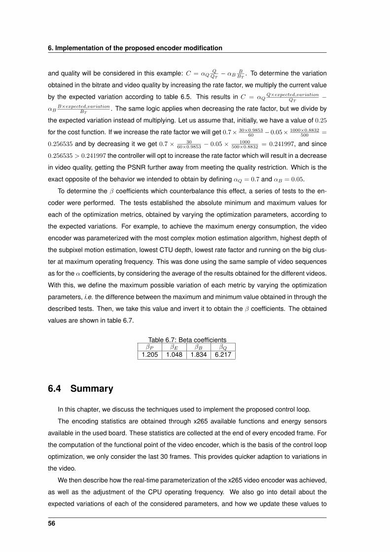
6. Implementation of the proposed encoder modification
and quality will be considered in this example: C = αQQQT
− αBBBT
. To determine the variation
obtained in the bitrate and video quality by increasing the rate factor, we multiply the current value
by the expected variation according to table 6.5. This results in C = αQQ×expected variation
QT−
αBB×expected variation
BT. The same logic applies when decreasing the rate factor, but we divide by
the expected variation instead of multiplying. Let us assume that, initially, we have a value of 0.25
for the cost function. If we increase the rate factor we will get 0.7× 30×0.985360 −0.05× 1000×0.8832
500 =
0.256535 and by decreasing it we get 0.7 × 3060×0.9853 − 0.05 × 1000
500×0.8832 = 0.241997, and since
0.256535 > 0.241997 the controller will opt to increase the rate factor which will result in a decrease
in video quality, getting the PSNR further away from meeting the quality restriction. Which is the
exact opposite of the behavior we intended to obtain by defining αQ = 0.7 and αB = 0.05.
To determine the β coefficients which counterbalance this effect, a series of tests to the en-
coder were performed. The tests established the absolute minimum and maximum values for
each of the optimization metrics, obtained by varying the optimization parameters, according to
the expected variations. For example, to achieve the maximum energy consumption, the video
encoder was parameterized with the most complex motion estimation algorithm, highest depth of
the subpixel motion estimation, lowest CTU depth, lowest rate factor and running on the big clus-
ter at maximum operating frequency. This was done using the same sample of video sequences
as for the α coefficients, by considering the average of the results obtained for the different videos.
With this, we define the maximum possible variation of each metric by varying the optimization
parameters, i.e. the difference between the maximum and minimum value obtained in through the
described tests. Then, we take this value and invert it to obtain the β coefficients. The obtained
values are shown in table 6.7.
Table 6.7: Beta coefficientsβP βE βB βQ
1.205 1.048 1.834 6.217
6.4 Summary
In this chapter, we discuss the techniques used to implement the proposed control loop.
The encoding statistics are obtained through x265 available functions and energy sensors
available in the used board. These statistics are collected at the end of every encoded frame. For
the computation of the functional point of the video encoder, which is the basis of the control loop
optimization, we only consider the last 30 frames. This provides quicker adaption to variations in
the video.
We then describe how the real-time parameterization of the x265 video encoder was achieved,
as well as the adjustment of the CPU operating frequency. We also go into detail about the
expected variations of each of the considered parameters, and how we update these values to
56

6.4 Summary
allow for a more dynamic optimization.
Finally, we describe how the cost function was parameterized in order to allow for optimization
profiles. In addition to the α coefficients, which define the priorities of each considered metric, we
also define β coefficients which normalize the different terms of the cost function, introduced to
ensure that the priorities defined with the α coefficients are followed.
57

6. Implementation of the proposed encoder modification
58

7Experimental Evaluation
Contents7.1 Testing framework . . . . . . . . . . . . . . . . . . . . . . . . . . . . . . . . . . . 607.2 Experimental results . . . . . . . . . . . . . . . . . . . . . . . . . . . . . . . . . 617.3 Control loop overhead . . . . . . . . . . . . . . . . . . . . . . . . . . . . . . . . 647.4 Summary . . . . . . . . . . . . . . . . . . . . . . . . . . . . . . . . . . . . . . . . 67
59
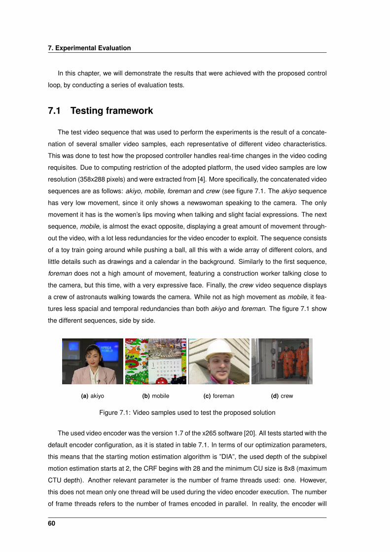
7. Experimental Evaluation
In this chapter, we will demonstrate the results that were achieved with the proposed control
loop, by conducting a series of evaluation tests.
7.1 Testing framework
The test video sequence that was used to perform the experiments is the result of a concate-
nation of several smaller video samples, each representative of different video characteristics.
This was done to test how the proposed controller handles real-time changes in the video coding
requisites. Due to computing restriction of the adopted platform, the used video samples are low
resolution (358x288 pixels) and were extracted from [4]. More specifically, the concatenated video
sequences are as follows: akiyo, mobile, foreman and crew (see figure 7.1. The akiyo sequence
has very low movement, since it only shows a newswoman speaking to the camera. The only
movement it has is the women’s lips moving when talking and slight facial expressions. The next
sequence, mobile, is almost the exact opposite, displaying a great amount of movement through-
out the video, with a lot less redundancies for the video encoder to exploit. The sequence consists
of a toy train going around while pushing a ball, all this with a wide array of different colors, and
little details such as drawings and a calendar in the background. Similarly to the first sequence,
foreman does not a high amount of movement, featuring a construction worker talking close to
the camera, but this time, with a very expressive face. Finally, the crew video sequence displays
a crew of astronauts walking towards the camera. While not as high movement as mobile, it fea-
tures less spacial and temporal redundancies than both akiyo and foreman. The figure 7.1 show
the different sequences, side by side.
(a) akiyo (b) mobile (c) foreman (d) crew
Figure 7.1: Video samples used to test the proposed solution
The used video encoder was the version 1.7 of the x265 software [20]. All tests started with the
default encoder configuration, as it is stated in table 7.1. In terms of our optimization parameters,
this means that the starting motion estimation algorithm is ”DIA”, the used depth of the subpixel
motion estimation starts at 2, the CRF begins with 28 and the minimum CU size is 8x8 (maximum
CTU depth). Another relevant parameter is the number of frame threads used: one. However,
this does not mean only one thread will be used during the video encoder execution. The number
of frame threads refers to the number of frames encoded in parallel. In reality, the encoder will
60
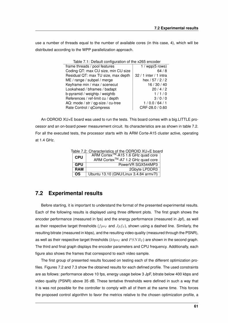
7.2 Experimental results
use a number of threads equal to the number of available cores (in this case, 4), which will be
distributed according to the WPP parallelization approach.
Table 7.1: Default configuration of the x265 encoderframe threads / pool features 1 / wpp(5 rows)Coding QT: max CU size, min CU size 64 / 8Residual QT: max TU size, max depth 32 / 1 inter / 1 intraME / range / subpel / merge hex / 57 / 2 / 2Keyframe min / max / scenecut 16 / 30 / 40Lookahead / bframes / badapt 20 / 4 / 2b-pyramid / weightp / weightb 1 / 1 / 0References / ref-limit cu / depth 3 / 0 / 0AQ: mode / str / qg-size / cu-tree 1 / 0.0 / 64 / 1Rate Control / qCompress CRF-28.0 / 0.60
An ODROID XU+E board was used to run the tests. This board comes with a big.LITTLE pro-
cessor and an on-board power measurement circuit. Its characteristics are as shown in table 7.2.
For all the executed tests, the processor starts with its ARM Corte-A15 cluster active, operating
at 1.4 GHz.
Table 7.2: Characteristics of the ODROID XU+E board
CPU ARM CortexTM-A15 1.6 GHz quad coreARM CortexTM-A7 1.2 GHz quad core
GPU PowerVR SGX544MP3RAM 2Gbyte LPDDR3OS Ubuntu 13.10 (GNU/Linux 3.4.84 armv7l)
7.2 Experimental results
Before starting, it is important to understand the format of the presented experimental results.
Each of the following results is displayed using three different plots. The first graph shows the
encoder performance (measured in fps) and the energy performance (measured in Jpf), as well
as their respective target thresholds (fpsT and JpfT ), shown using a dashed line. Similarly, the
resulting bitrate (measured in kbps), and the resulting video quality (measured through the PSNR),
as well as their respective target thresholds (kbpsT and PSNRT ) are shown in the second graph.
The third and final graph displays the encoder parameters and CPU frequency. Additionally, each
figure also shows the frames that correspond to each video sample.
The first group of presented results focused on testing each of the different optimization pro-
files. Figures 7.2 and 7.3 show the obtained results for each defined profile. The used constraints
are as follows: performance above 10 fps, energy usage below 3 JpF, bitrate below 400 kbps and
video quality (PSNR) above 35 dB. These tentative thresholds were defined in such a way that
it is was not possible for the controller to comply with all of them at the same time. This forces
the proposed control algorithm to favor the metrics relative to the chosen optimization profile, a
61
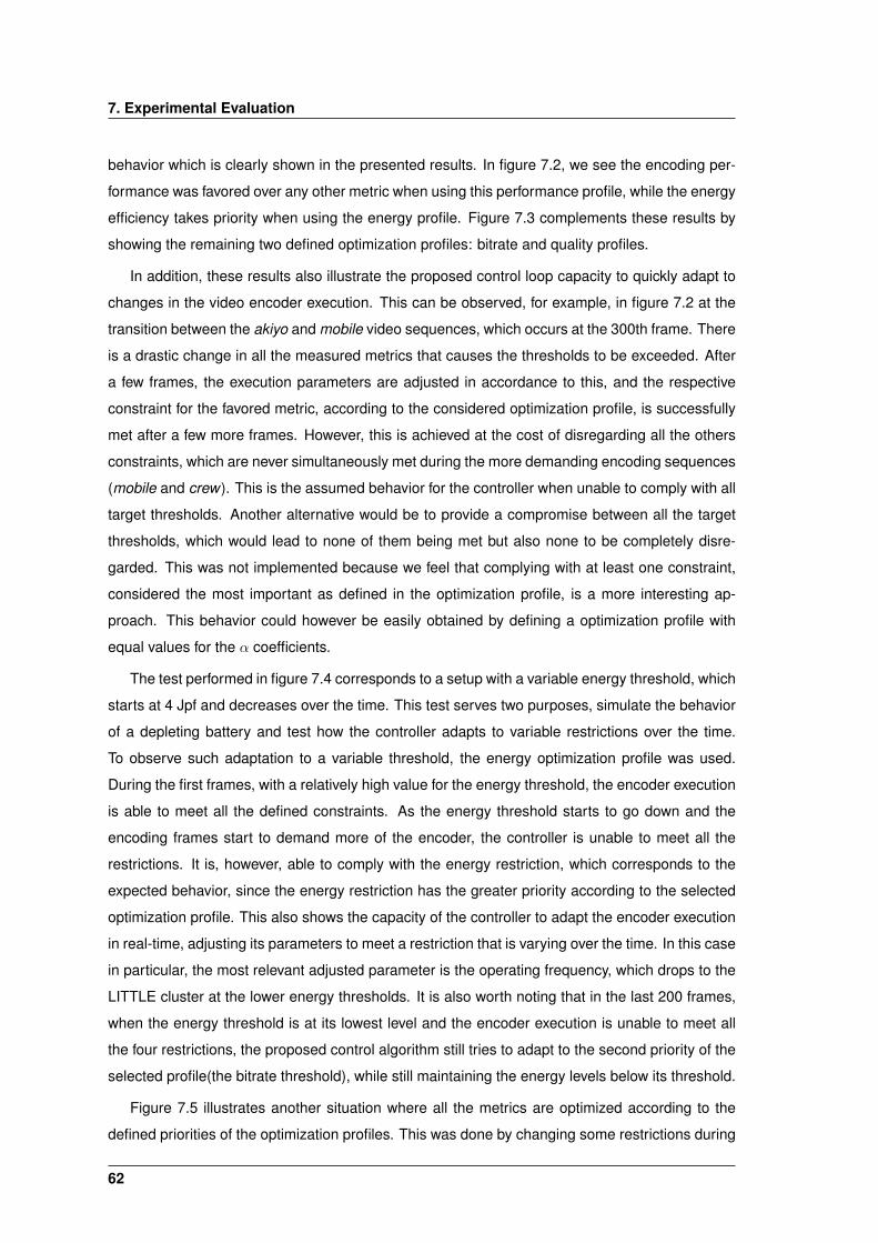
7. Experimental Evaluation
behavior which is clearly shown in the presented results. In figure 7.2, we see the encoding per-
formance was favored over any other metric when using this performance profile, while the energy
efficiency takes priority when using the energy profile. Figure 7.3 complements these results by
showing the remaining two defined optimization profiles: bitrate and quality profiles.
In addition, these results also illustrate the proposed control loop capacity to quickly adapt to
changes in the video encoder execution. This can be observed, for example, in figure 7.2 at the
transition between the akiyo and mobile video sequences, which occurs at the 300th frame. There
is a drastic change in all the measured metrics that causes the thresholds to be exceeded. After
a few frames, the execution parameters are adjusted in accordance to this, and the respective
constraint for the favored metric, according to the considered optimization profile, is successfully
met after a few more frames. However, this is achieved at the cost of disregarding all the others
constraints, which are never simultaneously met during the more demanding encoding sequences
(mobile and crew). This is the assumed behavior for the controller when unable to comply with all
target thresholds. Another alternative would be to provide a compromise between all the target
thresholds, which would lead to none of them being met but also none to be completely disre-
garded. This was not implemented because we feel that complying with at least one constraint,
considered the most important as defined in the optimization profile, is a more interesting ap-
proach. This behavior could however be easily obtained by defining a optimization profile with
equal values for the α coefficients.
The test performed in figure 7.4 corresponds to a setup with a variable energy threshold, which
starts at 4 Jpf and decreases over the time. This test serves two purposes, simulate the behavior
of a depleting battery and test how the controller adapts to variable restrictions over the time.
To observe such adaptation to a variable threshold, the energy optimization profile was used.
During the first frames, with a relatively high value for the energy threshold, the encoder execution
is able to meet all the defined constraints. As the energy threshold starts to go down and the
encoding frames start to demand more of the encoder, the controller is unable to meet all the
restrictions. It is, however, able to comply with the energy restriction, which corresponds to the
expected behavior, since the energy restriction has the greater priority according to the selected
optimization profile. This also shows the capacity of the controller to adapt the encoder execution
in real-time, adjusting its parameters to meet a restriction that is varying over the time. In this case
in particular, the most relevant adjusted parameter is the operating frequency, which drops to the
LITTLE cluster at the lower energy thresholds. It is also worth noting that in the last 200 frames,
when the energy threshold is at its lowest level and the encoder execution is unable to meet all
the four restrictions, the proposed control algorithm still tries to adapt to the second priority of the
selected profile(the bitrate threshold), while still maintaining the energy levels below its threshold.
Figure 7.5 illustrates another situation where all the metrics are optimized according to the
defined priorities of the optimization profiles. This was done by changing some restrictions during
62
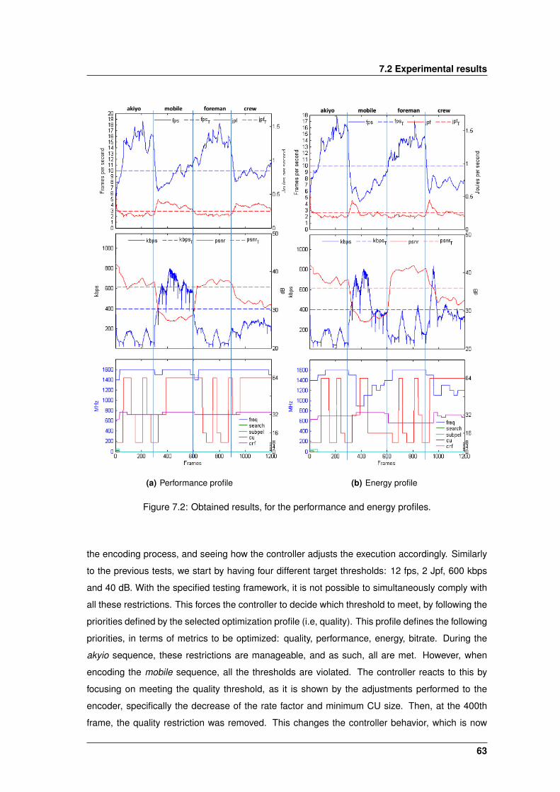
7.2 Experimental results
(a) Performance profile (b) Energy profile
Figure 7.2: Obtained results, for the performance and energy profiles.
the encoding process, and seeing how the controller adjusts the execution accordingly. Similarly
to the previous tests, we start by having four different target thresholds: 12 fps, 2 Jpf, 600 kbps
and 40 dB. With the specified testing framework, it is not possible to simultaneously comply with
all these restrictions. This forces the controller to decide which threshold to meet, by following the
priorities defined by the selected optimization profile (i.e, quality). This profile defines the following
priorities, in terms of metrics to be optimized: quality, performance, energy, bitrate. During the
akyio sequence, these restrictions are manageable, and as such, all are met. However, when
encoding the mobile sequence, all the thresholds are violated. The controller reacts to this by
focusing on meeting the quality threshold, as it is shown by the adjustments performed to the
encoder, specifically the decrease of the rate factor and minimum CU size. Then, at the 400th
frame, the quality restriction was removed. This changes the controller behavior, which is now
63
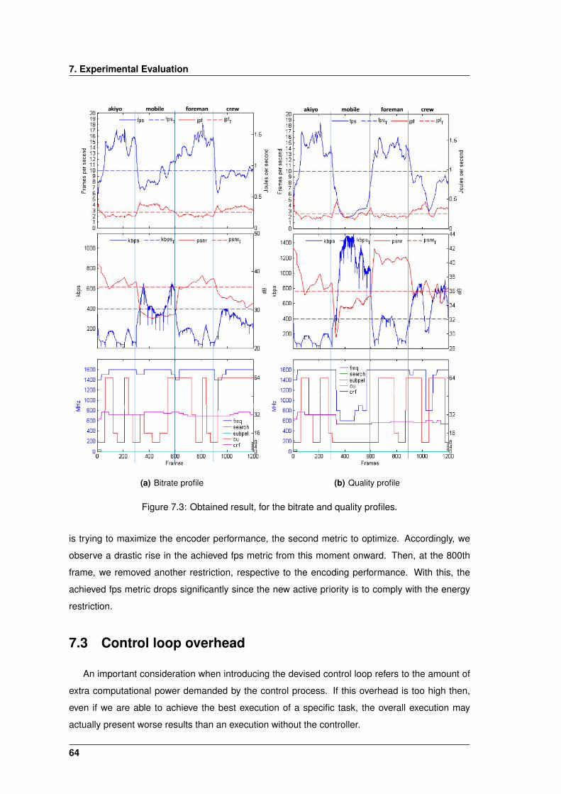
7. Experimental Evaluation
(a) Bitrate profile (b) Quality profile
Figure 7.3: Obtained result, for the bitrate and quality profiles.
is trying to maximize the encoder performance, the second metric to optimize. Accordingly, we
observe a drastic rise in the achieved fps metric from this moment onward. Then, at the 800th
frame, we removed another restriction, respective to the encoding performance. With this, the
achieved fps metric drops significantly since the new active priority is to comply with the energy
restriction.
7.3 Control loop overhead
An important consideration when introducing the devised control loop refers to the amount of
extra computational power demanded by the control process. If this overhead is too high then,
even if we are able to achieve the best execution of a specific task, the overall execution may
actually present worse results than an execution without the controller.
64
7.3 Control loop overhead
Figure 7.4: Obtained results when decreasing the targeted energy threshold
65
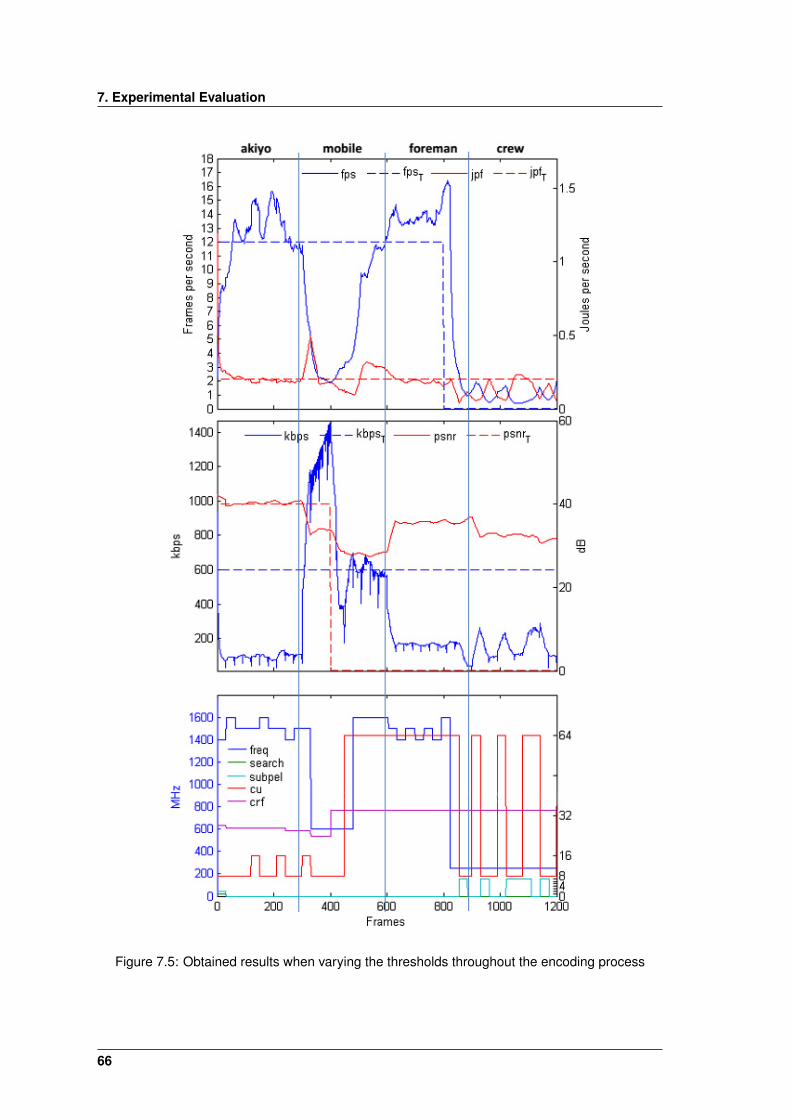
7. Experimental Evaluation
Figure 7.5: Obtained results when varying the thresholds throughout the encoding process
66
7.4 Summary
In the context of the proposed control loop, measuring this overhead is not as straightforward
as comparing the resulting execution with and without the controller. The reason for this is that our
control algorithm does not try to achieve the best possible performance or energy efficiency. What
it is actually achieved is the simultaneous compliance with the user defined restrictions, which
may cause the performance or energy efficiency to actually become lower (but still committing
the defined target thresholds) than the execution without the controller. It greatly depends on the
defined restrictions and selected optimization profile. With this in mind, we analyze the introduced
control loop overhead by measuring, during all the performed tests, the execution time elapsed
in control related tasks, such as computing the optimal functional point, performing adjustments
to the encoder or updating the expected variation. Through this analysis, we determined that,
the proposed control loop introduces an average overhead of 1.78 milliseconds per frame. This
corresponds to 1% of the execution time, an acceptable value for the introduced overhead.
7.4 Summary
To demonstrate the functionality of the proposed solution, several tests were conducted and
presented in this chapter. All experiments used the same video sequence, which results from the
concatenation of several video samples with distinct characteristics. The tests were performed
using an ODROID XU+E, running version 1.7 of the x265 HEVC video encoder.
The presented results successfully demonstrate the functionality of the proposed control al-
gorithm. It is shown that the controller is able to adapt, in real-time, to the existing variations in
the video characteristics and applied encoding restrictions. The obtained results also confirm that
the optimization process is able to prioritize different metrics, based on the selected optimization
profile.
67

7. Experimental Evaluation
68

8Conclusions
Contents8.1 Future work . . . . . . . . . . . . . . . . . . . . . . . . . . . . . . . . . . . . . . 70
69
8. Conclusions
This thesis presented an energy aware HEVC video encoder for mobile platforms. The need
for such an encoder comes growing from the penetration of video applications in mobile devices,
whose computational demands generally implies higher power consumption. However, since the
evolution of batteries has not been able to provide a significant boost in the available energy, the
need to increase the energy efficiency of these devices has focused the research of many teams
along the past few years. As a response to this, heterogeneous architectures aiming to ensure a
low energy consumption while still providing appreciable performance levels, are considered. One
of these architectures is the ARM big.LITTLE, used as the base platform to develop the proposed
control loop, which aims at providing an energy efficient video encoder.
Where the current state of the art is analyzed, we conclude that most of the current proposed
solutions for energy efficient HEVC in mobile platforms correspond to decoding solutions. In ad-
dition, most of these works fail to analyze the bitrate and video quality impact on the performance
and energy efficiency, and how these may be explored to further improve the video coding exe-
cution. In this work, we proposed a controller which is able not only to provide different levels of
performance and energy efficiency, but of bitrate and video quality as well.
The proposed control loop aims at dynamically adapting the x265 video encoder parameteriza-
tion to the imposed restrictions concerning the minimum encoding performance, energy efficiency,
bitrate and video quality. To achieve this, it exploits the big.LITTLE architecture, as well as the
real-time adjustment of some of the encoder parameters: motion estimation algorithm, subpixel
motion estimation depth, CTU depth and the CRF rate control method. Since we want to ensure
a dynamic control loop, which is able to continuously adapt to variations in the encoded video, the
adjustments that are applied to each parameter are updated throughout the encoding process.
It is also defined a set of optimization profiles, which aim at predefined priorities between the
metrics to optimize.
In order to validate the functionality of the proposed control algorithm, a series of tests were
performed with a video sequence characterized by a wide variability of its characteristics. the pro-
posed controller is able to simultaneously comply with several different restrictions, while adapting,
in real-time, to eventual variations in the input video or and to restrictions imposed by the outter
subsystem constraints. For the situations in which the controller is not able to meet all the thresh-
olds, it applies the defined optimization profile, which establishes priorities between the different
optimization metrics. Such a control loop demonstrated an overhead of about 1% of the overall
execution time, which is highly acceptable, considering the much greater video encoding effort.
8.1 Future work
There are some aspects of the presented work which may be further explored.
As it was previously mentioned, the big.LITTLE processor allows several types of task schedul-
70
8.1 Future work
ing. The scheduling type that was used in this work is based on cluster migration, which only al-
lows the migration of tasks between the big and LITTLE clusters, do not allowing the simultaneous
usage of both clusters. However, a more interesting task scheduling method to consider is the
”global task scheduling” (not available in the considered board), which is aware of each individual
core, allowing the simultaneously usage of all the available cores. It would enable asymmetrical
setups, for example, one big core and two LITTLE cores active, with all the others disabled. This
would also allow a better load balancing approach, assigning different type of encoding modules
to different types of cores. As an example, the more complex and demanding modules could be
assigned to the big cores, such as inter picture prediction, with other, less demanding modules,
assigned to the LITTLE cores.
Other aspect of this work which would benefit from further study is the controller and the
chosen set of parameters to adjust. In fact, the considered parameters were chosen based on
their impact on the relevant metrics of the encoder. Explore other parameters, which may have a
high impact in the encoder execution would provide a finer grained control algorithm, which would
lead to a more energy efficient execution.
71

8. Conclusions
72
Bibliography
[1] (Apr, 2016). http://www.videolan.org/developers/x264.html.
[2] (Apr, 2016). http://trac.ffmpeg.org/wiki/Encode/H.265.
[3] (Apr, 2016). http://slhck.info/articles/crf.
[4] (Apr, 2016). http://media.xiph.org/video/derf/.
[5] Ahn, Y.-J., Hwang, T.-J., Sim, D.-G., and Han, W.-J. (2014). Implementation of fast HEVC
encoder based on SIMD and data-level parallelism. EURASIP Journal on Image and Video
Processing, 2014(1):16.
[6] ARM (2013). big.LITTLE Technology: The Future of Mobile. ARM.
[7] Bossen, F., Bross, B., Member, S., Karsten, S., and Flynn, D. (2013). HEVC Complexity
and Implementation Analysis. Circuits and Systems for Video Technology, IEEE Transactions,
22(12):1685–1696.
[8] Cheung, N.-m., Fan, X., Au, O. C., and Kung, M.-c. (2010). Video Coding on Multicore Graph-
ics Processors. Signal Processing Magazine, IEEE, (March):79–89.
[9] Chi, C. C., Alvarez-mesa, M., Juurlink, B., Member, S., Clare, G., and Schierl, T. (2012).
Parallel Scalability and Efficiency of HEVC Parallelization Approaches. Circuits and Systems
for Video Technology, IEEE Transactions, 22(12):1827–1838.
[10] Cisco Systems, I. (2016). Cisco Visual Networking Index - Forecast and Methodology.
[11] Greenhalgh, P. (2012). big.LITTLE Processing with ARM Cortex-A15 & Cortex-A7. ARM,
(September 2011):1–8.
[12] He, Y., Kunstner, M., Gudumasu, S., Ryu, E. S., Ye, Y., and Xiu, X. (2013). Power aware
HEVC streaming for mobile. In Visual Communications and Image Processing (VCIP), 2013,
pages 1–5.
[13] Holmbacka, S., Nogues, E., Pelcat, M., Lafond, S., and Lilius, J. (2014). Energy efficiency
and performance management of parallel dataflow applications. In Design and Architectures
for Signal and Image Processing (DASIP), 2014 Conference on, pages 1–8.
73
Bibliography
[14] Jeff, B. (2012). Advances in big.LITTLE Technology for Power and Energy Savings. ARM,
(September):1–11.
[15] Lee, W. Y. (2012). Energy-efficient scheduling of periodic real-time tasks on lightly loaded
multicore processors. IEEE Transactions on Parallel and Distributed Systems, 23(3):530–537.
[16] Lee, W. Y., Ko, Y. W., Lee, H., and Kim, H. (2009). Energy-efficient scheduling of a real-
time task on dvfs-enabled multi-cores. In Proceedings of the 2009 International Conference on
Hybrid Information Technology, ICHIT ’09, pages 273–277. ACM.
[17] Momcilovic, S., Ilic, A., Roma, N., and Sousa, L. (2014). Dynamic Load Balancing for Real-
Time Video Encoding on Heterogeneous CPU + GPU Systems. Multimedia, IEEE Transactions,
16(1):108–121.
[18] Momcilovic, S., Roma, N., and Sousa, L. (2013). Exploiting task and data parallelism for ad-
vanced video coding on hybrid CPU+GPU platforms. Journal of Real-Time Image Processing.
[19] MulticoreWare (Apr, 2016a). http://x265.readthedocs.org/en/default/.
[20] MulticoreWare (Apr, 2016b). http://x265.org.
[21] Nogues, E., Berrada, R., Pelcat, M., Menard, D., and Raffin, E. (2015). A DVFS based HEVC
decoder for energy-efficient software implementation on embedded processors. Multimedia and
Expo (ICME), 2015 IEEE International Conference, pages 1–6.
[22] Nogues, E., Holmbacka, S., Pelcat, M., Menard, D., and Lilius, J. (2014). Power-aware
HEVC decoding with tunable image quality. In Signal Processing Systems (SiPS), 2014 IEEE
Workshop on, pages 1–6.
[23] Pricopi, M., Muthukaruppan, T. S., Venkataramani, V., Mitra, T., and Vishin, S. (2013).
Power-performance modeling on asymmetric multi-cores. 2013 International Conference on
Compilers, Architecture and Synthesis for Embedded Systems (CASES), pages 1–10.
[24] Raffin, E., Nogues, E., Hamidouche, W., Tomperi, S., Pelcat, M., and Menard, D. (2015). Low
power HEVC software decoder for mobile devices. Journal of Real-Time Image Processing,
pages 1–13.
[25] Randhawa, R. and Engineer, P. (2013). Software Techniques for ARM big.LITTLE Systems.
ARM, (April).
[26] Rodrıguez, A., Gonzalez, A., and Malumbres, M. P. (2006). Hierarchical Parallelization of
an H.264/AVC Video Encoder. Parallel Computing in Electrical Engineering, 2006. PAR ELEC
2006. International Symposium on.
74
Bibliography
[27] Rodrıguez-Sanchez, R. and Quintana-Ortı, E. S. (2016). Architecture-aware optimization of
an HEVC decoder on asymmetric multicore processors. CoRR, abs/1601.05313.
[28] Rountree, B., Lownenthal, D. K., de Supinski, B. R., Schulz, M., Freeh, V. W., and Bletsch, T.
(2009). Adagio: Making dvs practical for complex hpc applications. In Proceedings of the 23rd
International Conference on Supercomputing, ICS ’09, pages 460–469.
[29] Sankaraiah, S., La, H. S., Eswaran, C., and Abdullah, J. (2011). GOP Level Parallelism
on H.264 Video Encoder for Multicore Architecture. International Proceedings of Computer
Science and Information Technology, 7:127–132.
[30] Sullivan, G. J., Ohm, J.-r., Han, W.-j., and Wiegand, T. (2012). Overview of the High Efficiency
Video Coding. Circuits and Systems for Video Technology, IEEE Transactions, 22(12):1649–
1668.
[31] Wien, M. (2015). High Efficiency Video Coding - Coding Tools and Specification. Circuits
and Systems for Video Technology, IEEE Transactions.
[32] Zhao, Z., Liang, P., and Member, S. (2006). Data Partition for Wavefront Parallelization of
H . 264 Video Encoder. Circuits and Systems, 2006. ISCAS 2006. Proceedings. 2006 IEEE
International Symposium on, pages 2669–2672.
75

Bibliography
76

Bibliography
77