NCHRP IDEA Program

Bidirectional-Ductile End Diaphragms for Seismic Performance and

Substructure Protection

Final Report for

NCHRP IDEA Project 172

Prepared by:

Xiaone Wei and Michel Bruneau

University at Buffalo

November 2015

Innovations Deserving Exploratory Analysis (IDEA) Programs

Managed by the Transportation Research Board

This IDEA project was funded by the NCHRP IDEA Program.

The TRB currently manages the following three IDEA programs:

The NCHRP IDEA Program, which focuses on advances in the design, construction, and

maintenance of highway systems, is funded by American Association of State Highway and

Transportation Officials (AASHTO) as part of the National Cooperative Highway Research

Program (NCHRP).

The Safety IDEA Program currently focuses on innovative approaches for improving railroad

safety or performance. The program is currently funded by the Federal Railroad

Administration (FRA). The program was previously jointly funded by the Federal Motor

Carrier Safety Administration (FMCSA) and the FRA.

The Transit IDEA Program, which supports development and testing of innovative concepts

and methods for advancing transit practice, is funded by the Federal Transit Administration

(FTA) as part of the Transit Cooperative Research Program (TCRP).

Management of the three IDEA programs is coordinated to promote the development and testing

of innovative concepts, methods, and technologies.

For information on the IDEA programs, check the IDEA website (www.trb.org/idea). For

questions, contact the IDEA programs office by telephone at (202) 334-3310.

IDEA Programs

Transportation Research Board

500 Fifth Street, NW

Washington, DC 20001

The project that is the subject of this contractor-authored report was a part of the Innovations Deserving

Exploratory Analysis (IDEA) Programs, which are managed by the Transportation Research Board

(TRB) with the approval of the National Academies of Sciences, Engineering, and Medicine. The

members of the oversight committee that monitored the project and reviewed the report were chosen for

their special competencies and with regard for appropriate balance. The views expressed in this report

are those of the contractor who conducted the investigation documented in this report and do not

necessarily reflect those of the Transportation Research Board; the National Academies of Sciences,

Engineering, and Medicine; or the sponsors of the IDEA Programs.

The Transportation Research Board; the National Academies of Sciences, Engineering, and Medicine;

and the organizations that sponsor the IDEA Programs do not endorse products or manufacturers. Trade

or manufacturers’ names appear herein solely because they are considered essential to the object of the

investigation.

Bidirectional-Ductile End Diaphragms for Seismic Performance and

Substructure Protection

NCHRP IDEA Project 172

Final Report

Prepared for the NCHRP IDEA Program

Transportation Research Board

The National Academies

Xiaone Wei and Michel Bruneau

University at Buffalo

November 2015

ACKNOWLEDGEMENTS

This work was funded by the Transportation Research Board of the National Academies under the TRB-IDEA

Program (NCHRP-172). Special thanks is extended by the Research Team to the TRB Project Director, Inam

Jawed, and the Advisory Panel: Lian Duan, California Department of Transportation; Fred Faridazar, Federal

Highway Administration; Bijan Khaleghi, Washington Department of Transportation ; Richard Marchione,

New York Department of Transportation; Tom Ostrom, California Department of Transportation; Geoff Swett,

Washington Department of Transportation; Rajesh Taneja, New York Department of Transportation; W.

Phillip Yen, Federal Highway Administration.

The generous donation of the specimens used in this project from Star Seismic is greatly appreciated.

Experimental work for this project was conducted at the Structural Engineering and Earthquake Simulation

Laboratory at University at Buffalo.

i

NCHRP IDEA PROGRAM COMMITTEE

CHAIR

DUANE BRAUTIGAM

Consultant

MEMBERS

CAMILLE CRICHTON-SUMNERS

New Jersey DOT

AGELIKI ELEFTERIADOU

University of Florida

ANNE ELLIS

Arizona DOT

ALLISON HARDT

Maryland State Highway Administration

JOE HORTON

California DOT

MAGDY MIKHAIL

Texas DOT TOMMY NANTUNG

Indiana DOT

MARTIN PIETRUCHA

Pennsylvania State University

VALERIE SHUMAN Shuman Consulting Group LLC

L.DAVID SUITS North American Geosynthetics Society

JOYCE TAYLOR

Maine DOT

FHWA LIAISON DAVID KUEHN

Federal Highway Administration

TRB LIAISON

RICHARD CUNARD

Transportation Research Board

COOPERATIVE RESEARCH PROGRAM STAFF

STEPHEN PARKER

Senior Program Officer

IDEA PROGRAMS STAFF STEPHEN R. GODWIN

Director for Studies and Special Programs

JON M. WILLIAMS

Program Director, IDEA and Synthesis Studies

INAM JAWED

Senior Program Officer DEMISHA WILLIAMS

Senior Program Assistant

EXPERT REVIEW PANEL

LIAN DUAN, California DOT FRED FARIDAZAR, FHWA

BIJAN KHALEGHI, Washington DOT

RICHARD MARCHIONE, New York DOT

TOM OSTROM, California DOT

GEOFF SWETT, Washington DOT

RAJESH TANEJA, New York DOT

W.PHILLIP YEN, FHWA

ii

TABLE OF CONTENTS

1 EXECUTIVE SUMMARY ........................................................................................................................................ 1

2 IDEA PRODUCT .............................................................................................................................................. 2

3 CONCEPT AND INNOVATIONS ............................................................................................................................ 2

4 INVESTIGATION ............................................................................................................................................. 3

4.1 General ................................................................................................................................................. 3

4.2 Stage 1-Parametric dynamic analyses and low-cycle fatigue study ...................................................... 3

4.2.1 Parametric Dynamic Analyses ............................................................................................................ 3

4.2.1.1 Benchmark Models ................................................................................................................... 3

4.2.1.2 Nonlinear time history analysis of non-skew and skew bridges ............................................... 4

4.2.2 Thermal Effect on the Low-cycle Fatigue of BRBs ............................................................................. 9

4.3 Stage 2-Experimental Investigation .................................................................................................... 10

4.3.1 Test Set-up and BRB Specimens .................................................................................................. 11

4.3.2 Instrumentation .......................................................................................................................... 13

4.3.3 BRB Displacement Demands and Test Protocols ........................................................................ 14

4.3.3.1 BRB Bidirectional Displacement Demands .............................................................................. 14

4.3.3.2 BRB Bidirectional Qualification Test Protocols ........................................................................ 16

4.3.3.3 BRB Temperature-induced Axial Displacement Demands and Protocol ................................. 18

4.3.3.4 BRB Test Protocol Summary ........................................................................................................19

4.3.4 Example BRB Tests ...................................................................................................................... 20

4.3.4.1 BRB-2-4 ................................................................................................................................... 20

4.3.4.2 BRB-1-3 ................................................................................................................................... 23

4.3.5 Investigation on BRB Test Results ............................................................................................... 27

4.3.5.1 Observations on BRB’s failure ......................................................................................................27

4.3.5.2 Cumulative Inelastic Deformations ......................................................................................... 29

4.3.5.3 Low-cycle Fatigue Damage ...................................................................................................... 30

4.4 Design Procedures .............................................................................................................................. 31

5 FINDINGS AND CONCLUSIONS ..........................................................................................................................32

6 PLANS FOR IMPLEMENTATION ................................................................................................................... 33

7 REFERENCES ................................................................................................................................................ 33

1

1 EXECUTIVE SUMMARY

The AASHTO Guide Specifications for LRFD Seismic Bridge Design (2011) include provisions for the

design of steel bridges having specially detailed ductile diaphragms to resist loads applied in the bridge’s

transverse direction. However, a major limitation of the existing provisions is that those ductile diaphragms

have to be combined with other lateral-load resisting strategies to address seismic excitations acting along the

bridge’s longitudinal axis. Furthermore, these design provisions for ductile diaphragms are only applicable to

non-skew bridges and provide no guidance on how to implement ductile diaphragms in skew bridges.

A bi-directional ductile end diaphragm concept has been proposed here to implement ductile end diaphragms

in straight or skew bridge superstructures. The proposed concept relies on easily replaceable hysteretic energy

dissipating devices (structural fuses) arrayed such as to provide ductile response to horizontal bidirectional

earthquake excitations. Buckling Restrained Braces (BRBs) are explored here as a possible solution to serve

as the ductile diaphragm’s seismic fuses.

In Stage 1 of this research project (described in Section 4.2), bidirectional ductile end diaphragm systems were

designed for benchmark skew and non-skew bridges and analyzed using nonlinear time history analysis to

examine their seismic performance. Variations in skew, fundamental period of vibration, and earthquake

excitation characteristics were also considered. These dynamic analyses allowed investigating the impact of

these parameters on global behavior, as well as understanding the magnitude of local demands and the extent

of bidirectional displacements that the BRBs must be able to accommodate while delivering their ductile

response. The long-term service life of BRBs installed across expansion joints and subjected to bridge thermal

expansion histories was also investigated and a minimum ratio of the BRB’s core over the whole bridge

length was recommended.

In Stage 2 of this research project (described in Section 4.3), quasi-static experiments were conducted to

subject BRBs to a regime of relative end-displacements representative of the results predicted from the Stage

1’s parametric analytical studies. In each test, one end of the BRB was connected to a reaction block tied down

to holes in the laboratory’s strong floor, while the other end was connected to a shake table that was used

to apply horizontal bidirectional end displacement demands to the BRB. The loading protocols included

bidirectional displacement histories to subject the specimens to large inelastic deformation cycles, and uniaxial

displacement histories to investigate the low-cycle fatigue due to temperature changes. Two types of BRBs

having flat end plates and unidirectional pinholes were designed, namely BRB-1 and BRB-2. The end plates

of BRB-1 were designed to bend laterally to accommodate the lateral displacements. The end plates of BRB-2

were connected to a spherical bearing (similar to those used by some damper manufacturers) installed in the

gusset plate to which the BRB was connected. Four specimens of each BRB type were subjected to different

combinations of displacement protocols. The BRB’s hysteretic behaviors under different displacement

protocols were studied and compared. The ultimate behavior of a BRB was typically quantified in terms of

t h e cumulative inelastic deformations that the BRB’s core plate experienced during the tests. The BRB

specimens tested typically developed cumulative inelastic deformations of more than 250 times the BRB’s

axial yield displacement, including multiple years of severe temperature cycles (it is believed that other BRBs

designs could most significantly increase this limit). Ultimately, as expected, all the BRBs failed in tension

(where the BRB’s internal core plate locally buckled the most) after extensive cycles of inelastic deformations.

No end-plate failure or instability was observed (which would have been undesirable failure modes).

Detailed analyses of cumulative inelastic deformations and low-cycle fatigue life of all BRBs using data from

the experiments were performed. A recommended design procedure in Section 4.4 for the EDSs in both non-

skew and skew bridges was developed based on the paramedic analyses and experimental results.

2

2 IDEA PRODUCT

By providing an analytically and experimentally proven solution for ductile diaphragms able to explicitly

address the fact that earthquake simultaneously shake a bridge in all horizontal directions (not just transversely

to the bridge axis), and by making this solution also applicable to skew bridges (a large percentage of all

bridges), this research is therefore poised to make ductile diaphragms a commonly used seismic-resistance

solution for most short and medium span steel bridges in all seismic regions (i.e. in regions exposed to low

levels of seismicity, ranging up to those exposed to more severe earthquakes). Although the proposed research

was conducted in the perspective of new bridge design, the information generated by this project will be

equally applicable to existing bridges for seismic retrofit purposes.

3 CONCEPT AND INNOVATIONS

A bidirectional ductile end diaphragm concept was proposed to implement ductile end diaphragms in straight or

skew bridge superstructures, to resist bidirectional earthquake excitations. The AASHTO Guide

Specifications for LRFD Seismic Bridge Design (2011) already include provisions for the design of steel

bridges having specially detailed ductile diaphragms, but these are only applicable to straight bridges without

skew, and only provide resistance to earthquake excitations acting in the direction transverse to the bridge axis.

This is a most serious limitation and a real impediment to the implementation of ductile diaphragms. Without

addressing the issues of skew and bi-directionality, implementations of the ductile diaphragm concept would

remain limited (or rare), which is most unfortunate because ductile diaphragms are a low cost seismic solution

compared to other alternatives.

The proposed concept relies on hysteretic energy dissipation devices, which are structural fuses intended to be

easily replaceable devices, arrayed such as to provide ductile response to horizontal earthquake excitations

acting from any direction. Two end diaphragm systems (EDSs) (i.e. geometrical layouts) are proposed,

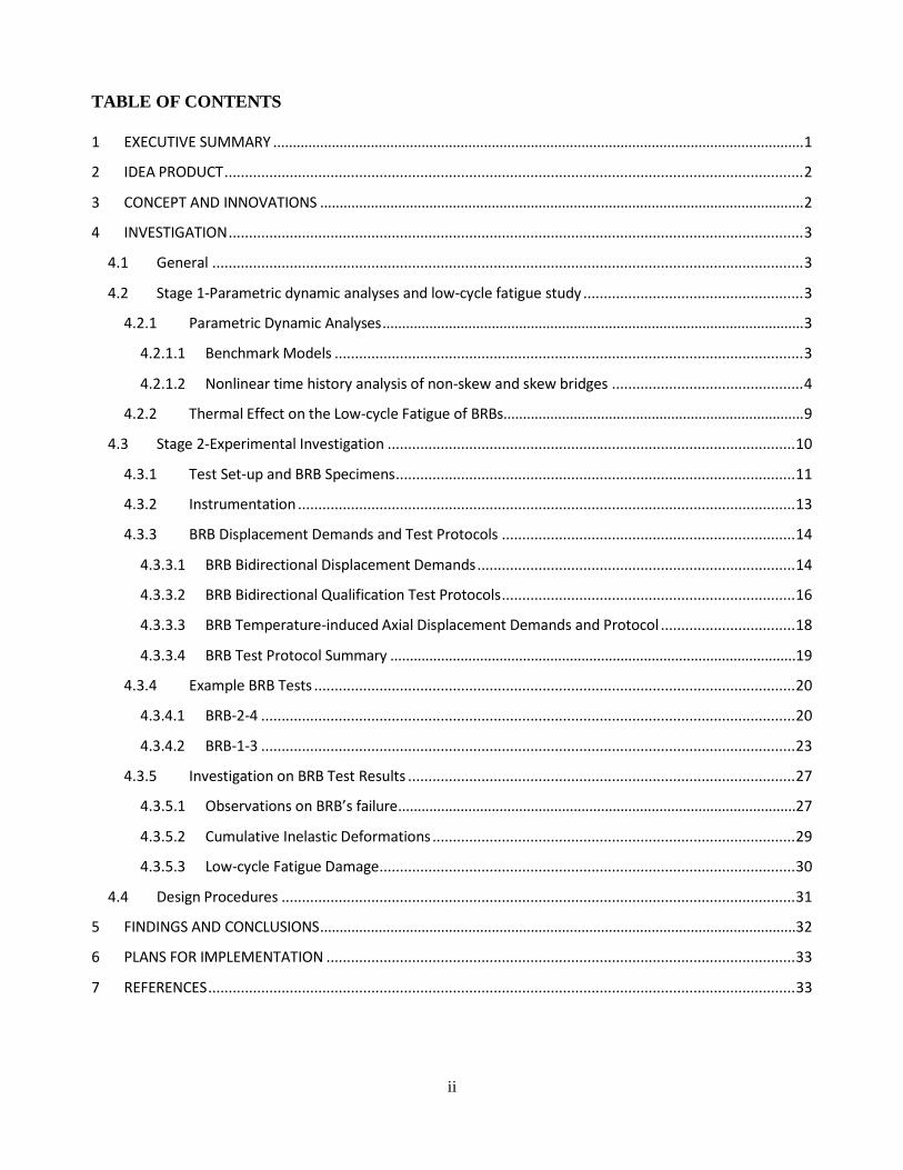
namely EDS-1 and EDS-2 (Fig. 1), described as follows:

End Diaphragm System-1 (EDS-1): Two pairs of structural fuses installed at each end of a span, in

a configuration that coincides with the skew and longitudinal directions.

End Diaphragm System-2 (EDS-2): A single pair of structural fuses installed at each end of a span,

at angles that do not coincide with the bridge longitudinal and skew directions.

Buckling Restrained Braces (BRBs) were chosen here as a possible solution to serve as the diaphragm’s

ductile seismic fuses (other hysteretic energy dissipation devices could equally work for this purpose). BRBs

have been implemented in many buildings and bridges on account of their stable unpinched hysteretic

characteristics, ease of design, and ability to eliminate seismically-induced structural damage and provide

satisfactory seismic performance (AISC 2010, Bruneau et al. 2011). BRBs have also been used to retrofit the

Minato bridge in Japan (Kanaji et al. 2003), the world’s third longest truss bridge, using a concept similar to

the ductile cross frame system developed by Sarraf and Bruneau (1998a,b) and analogous to the ductile

diaphragm concept.

3

FIGURE 1 Proposed schemes for bridge ductile end diaphragms systems (EDS): (a) EDS-1; (b) EDS-2.

4 INVESTIGATION

4.1 General

The investigation included two stages of work, and information in this report is presented as follows:

(1) Stage 1 in Section 4.2: Dynamic parametric analyses of chosen configurations of EDS-1 and EDS-2 in

Section 4.2.1; low-cycle fatigue study of BRBs due to temperature change in Section 4.2.2

(2) Stage 2 in Section 4.3: Development of connection details of BRBs and test setup information in Section

4.3.1; instrumentation of the BRB tests in Section 4.3.2; BRB test protocols in Section 4.3.3; example

BRB test results in Section 4.3.4; investigation of the BRB test results in Section 4.3.5

(3) Proposed design procedures for the bidirectional ductile diaphragm in Section 4.4

4.2 Stage 1—Parametric Dynamic Analyses and Low-Cycle Fatigue Study

4.2.1 Parametric dynamic analyses

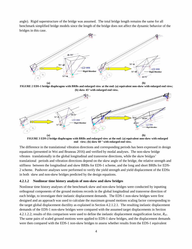
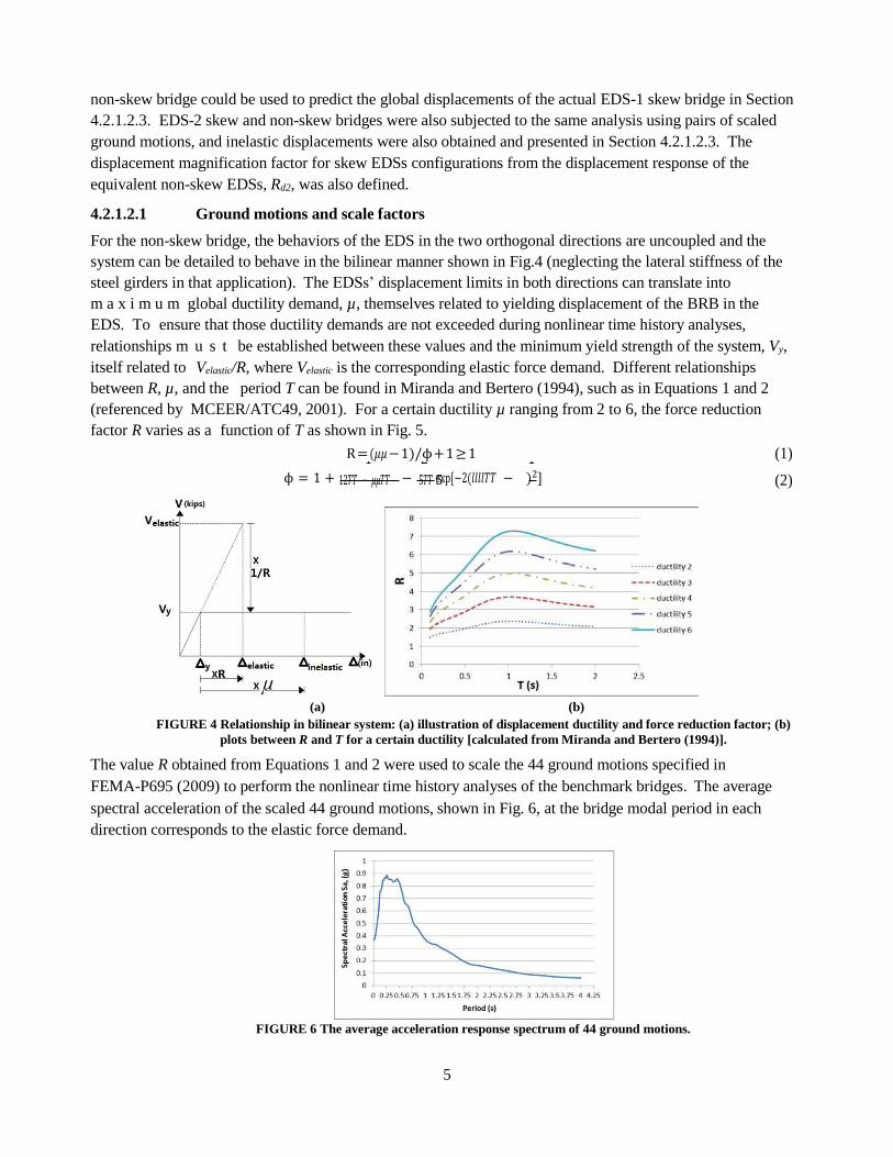
4.2.1.1 Benchmark models

Benchmark simplified bridge models with two EDSs have been developed in SAP2000 Version 14 and

OpenSees Version 2.4.6. These benchmark bridge models were used in the nonlinear time history analysis to

study dynamic behaviors of the proposed EDSs. Both skew and non-skew bridges were modeled, and the

skew angles of the bridges were changed at a 15 degree interval from 0 to 75 degree. The key dimensions of

the EDSs are the girder skew spacing projection in the transverse direction, s, end diaphragm depth, d, which

is approximately equal to the girder depth, and the horizontal longitudinal distance between connections of

the longitudinal BRB at deck level and the abutment, a. The skew and non-skew bridge models have the

same yield strength and yield displacement in both the longitudinal and transverse directions for the two EDS

schemes. For EDS-1 scheme shown in Fig. 2, the three dimensions mentioned above are equal for all skew

and non-skew bridges. For EDS-2 scheme shown in Fig. 3, the parameter s and d are the same, while the

parameter a is selected such as to make the longitudinal and transverse yield strength and displacement of the

skew EDS the same as for the equivalent non-skew EDS (note that a will change as a function of the skew

4

angle). Rigid superstructure of the bridge was assumed. The total bridge length remains the same for all

benchmark simplified bridge models since the length of the bridge does not affect the dynamic behavior of the

bridges in this case.

(a) (b)

FIGURE 2 EDS-1 bridge diaphragms with BRBs and enlarged view at the end: (a) equivalent non-skew with enlarged end view;

(b) skew 45° with enlarged end view.

(a) (b)

FIGURE 3 EDS-2 bridge diaphragms with BRBs and enlarged view at the end: (a) equivalent non-skew with enlarged

end view; (b) skew 60 ° with enlarged end view.

The difference in the translational vibration directions and corresponding periods has been expressed in design

equations (presented in Wei and Bruneau 2016) and verified by modal analyses. The non-skew bridge

vibrates translationally in the global longitudinal and transverse directions, while the skew bridges’

translational periods and vibration directions depend on the skew angle of the bridge, the relative strength and

stiffness between the longitudinal and skew BRBs for EDS-1 scheme, and the long and short BRBs for EDS-

2 scheme. Pushover analyses were performed to verify the yield strength and yield displacement of the EDSs

in both skew and non-skew bridges predicted by the design equations.

4.2.1.2 Nonlinear time history analysis of non-skew and skew bridges

Nonlinear time history analyses of the benchmark skew and non-skew bridges were conducted by inputting

orthogonal components of the ground motions records in the global longitudinal and transverse direction of

each bridge, to investigate their inelastic displacement demands. The EDS-1 non-skew bridges were first

designed and an approach was used to calculate the maximum ground motions scaling factor corresponding to

the target global displacement ductility as explained in Section 4.2.1.2.1. The resulting inelastic displacement

demands of the EDS-1 non-skew bridges were compared with the assumed target displacements in Section

4.2.1.2.2; results of this comparison were used to define the inelastic displacement magnification factor, Rd1.

The same pairs of scaled ground motions were applied to EDS-1 skew bridges, and the displacement demands

were then compared with the EDS-1 non-skew bridges to assess whether results from the EDS-1 equivalent

5

non-skew bridge could be used to predict the global displacements of the actual EDS-1 skew bridge in Section

4.2.1.2.3. EDS-2 skew and non-skew bridges were also subjected to the same analysis using pairs of scaled

ground motions, and inelastic displacements were also obtained and presented in Section 4.2.1.2.3. The

displacement magnification factor for skew EDSs configurations from the displacement response of the

equivalent non-skew EDSs, Rd2, was also defined.

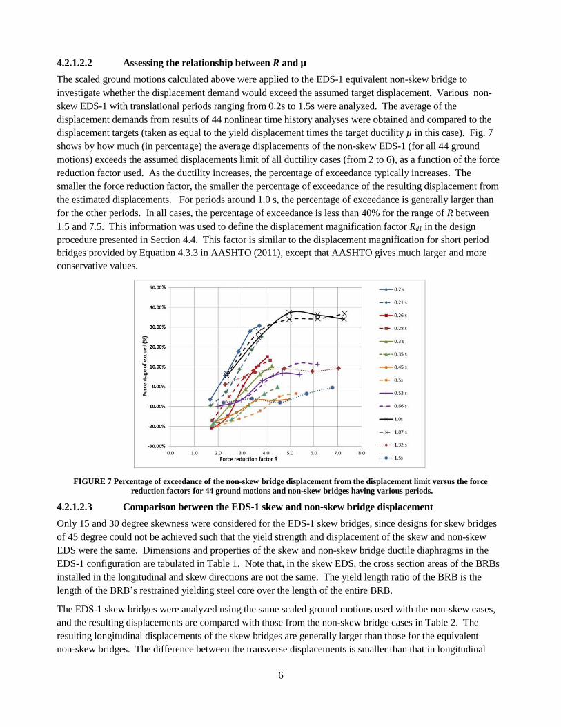
4.2.1.2.1 Ground motions and scale factors

For the non-skew bridge, the behaviors of the EDS in the two orthogonal directions are uncoupled and the

system can be detailed to behave in the bilinear manner shown in Fig.4 (neglecting the lateral stiffness of the

steel girders in that application). The EDSs’ displacement limits in both directions can translate into

m a x i m u m global ductility demand, µ, themselves related to yielding displacement of the BRB in the

EDS. To ensure that those ductility demands are not exceeded during nonlinear time history analyses,

relationships m u s t be established between these values and the minimum yield strength of the system, Vy,

itself related to Velastic/R, where Velastic is the corresponding elastic force demand. Different relationships

between R, µ, and the period T can be found in Miranda and Bertero (1994), such as in Equations 1 and 2

(referenced by MCEER/ATC49, 2001). For a certain ductility µ ranging from 2 to 6, the force reduction

factor R varies as a function of T as shown in Fig. 5.

(a) (b)

FIGURE 4 Relationship in bilinear system: (a) illustration of displacement ductility and force reduction factor; (b)

plots between R and T for a certain ductility [calculated from Miranda and Bertero (1994)].

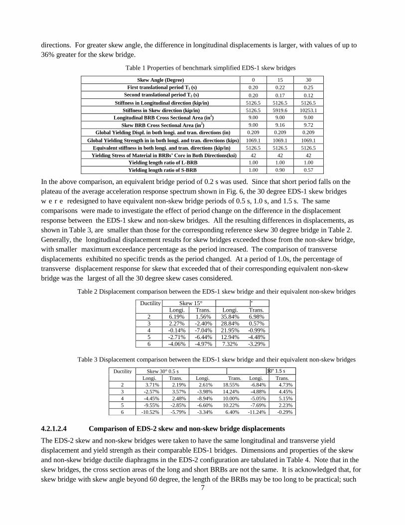
The value R obtained from Equations 1 and 2 were used to scale the 44 ground motions specified in

FEMA-P695 (2009) to perform the nonlinear time history analyses of the benchmark bridges. The average

spectral acceleration of the scaled 44 ground motions, shown in Fig. 6, at the bridge modal period in each

direction corresponds to the elastic force demand.

FIGURE 6 The average acceleration response spectrum of 44 ground motions.

R = (𝜇𝜇 − 1)/ϕ + 1 ≥ 1 (1) 1 2 1

ϕ = 1 + − exp[−2(𝑙𝑙𝑙𝑙𝑇𝑇 − )2] 12𝑇𝑇 − 𝜇𝜇𝑇𝑇 5𝑇𝑇 5 (2)

6

4.2.1.2.2 Assessing the relationship between R and µ

The scaled ground motions calculated above were applied to the EDS-1 equivalent non-skew bridge to

investigate whether the displacement demand would exceed the assumed target displacement. Various non-

skew EDS-1 with translational periods ranging from 0.2s to 1.5s were analyzed. The average of the

displacement demands from results of 44 nonlinear time history analyses were obtained and compared to the

displacement targets (taken as equal to the yield displacement times the target ductility µ in this case). Fig. 7

shows by how much (in percentage) the average displacements of the non-skew EDS-1 (for all 44 ground

motions) exceeds the assumed displacements limit of all ductility cases (from 2 to 6), as a function of the force

reduction factor used. As the ductility increases, the percentage of exceedance typically increases. The

smaller the force reduction factor, the smaller the percentage of exceedance of the resulting displacement from

the estimated displacements. For periods around 1.0 s, the percentage of exceedance is generally larger than

for the other periods. In all cases, the percentage of exceedance is less than 40% for the range of R between

1.5 and 7.5. This information was used to define the displacement magnification factor Rd1 in the design

procedure presented in Section 4.4. This factor is similar to the displacement magnification for short period

bridges provided by Equation 4.3.3 in AASHTO (2011), except that AASHTO gives much larger and more

conservative values.

FIGURE 7 Percentage of exceedance of the non-skew bridge displacement from the displacement limit versus the force

reduction factors for 44 ground motions and non-skew bridges having various periods.

4.2.1.2.3 Comparison between the EDS-1 skew and non-skew bridge displacement

Only 15 and 30 degree skewness were considered for the EDS-1 skew bridges, since designs for skew bridges

of 45 degree could not be achieved such that the yield strength and displacement of the skew and non-skew

EDS were the same. Dimensions and properties of the skew and non-skew bridge ductile diaphragms in the

EDS-1 configuration are tabulated in Table 1. Note that, in the skew EDS, the cross section areas of the BRBs

installed in the longitudinal and skew directions are not the same. The yield length ratio of the BRB is the

length of the BRB’s restrained yielding steel core over the length of the entire BRB.

The EDS-1 skew bridges were analyzed using the same scaled ground motions used with the non-skew cases,

and the resulting displacements are compared with those from the non-skew bridge cases in Table 2. The

resulting longitudinal displacements of the skew bridges are generally larger than those for the equivalent

non-skew bridges. The difference between the transverse displacements is smaller than that in longitudinal

7

directions. For greater skew angle, the difference in longitudinal displacements is larger, with values of up to

36% greater for the skew bridge.

Table 1 Properties of benchmark simplified EDS-1 skew bridges

Skew Angle (Degree) 0 15 30

First translational period T1 (s) 0.20 0.22 0.25

Second translational period T2 (s) 0.20 0.17 0.12

Stiffness in Longitudinal direction (kip/in) 5126.5 5126.5 5126.5

Stiffness in Skew direction (kip/in) 5126.5 5919.6 10253.1

Longitudinal BRB Cross Sectional Area (in2) 9.00 9.00 9.00

Skew BRB Cross Sectional Area (in2) 9.00 9.16 9.72

Global Yielding Displ. in both longi. and tran. directions (in) 0.209 0.209 0.209

Global Yielding Strength in in both longi. and tran. directions (kips) 1069.1 1069.1 1069.1

Equivalent stiffness in both longi. and tran. directions (kip/in) 5126.5 5126.5 5126.5

Yielding Stress of Material in BRBs’ Core in Both Directions(ksi) 42 42 42

Yielding length ratio of L-BRB 1.00 1.00 1.00

Yielding length ratio of S-BRB 1.00 0.90 0.57

In the above comparison, an equivalent bridge period of 0.2 s was used. Since that short period falls on the

plateau of the average acceleration response spectrum shown in Fig. 6, the 30 degree EDS-1 skew bridges

w e r e redesigned to have equivalent non-skew bridge periods of 0.5 s, 1.0 s, and 1.5 s. The same

comparisons were made to investigate the effect of period change on the difference in the displacement

response between the EDS-1 skew and non-skew bridges. All the resulting differences in displacements, as

shown in Table 3, are smaller than those for the corresponding reference skew 30 degree bridge in Table 2.

Generally, the longitudinal displacement results for skew bridges exceeded those from the non-skew bridge,

with smaller maximum exceedance percentage as the period increased. The comparison of transverse

displacements exhibited no specific trends as the period changed. At a period of 1.0s, the percentage of

transverse displacement response for skew that exceeded that of their corresponding equivalent non-skew

bridge was the largest of all the 30 degree skew cases considered.

Table 2 Displacement comparison between the EDS-1 skew bridge and their equivalent non-skew bridges

°

Table 3 Displacement comparison between the EDS-1 skew bridge and their equivalent non-skew bridges

30° 1.5 s

4.2.1.2.4 Comparison of EDS-2 skew and non-skew bridge displacements

The EDS-2 skew and non-skew bridges were taken to have the same longitudinal and transverse yield

displacement and yield strength as their comparable EDS-1 bridges. Dimensions and properties of the skew

and non-skew bridge ductile diaphragms in the EDS-2 configuration are tabulated in Table 4. Note that in the

skew bridges, the cross section areas of the long and short BRBs are not the same. It is acknowledged that, for

skew bridge with skew angle beyond 60 degree, the length of the BRBs may be too long to be practical; such

Ductility Skew 15° Longi. Trans. Longi. Trans.

2 6.19% 1.56% 35.84% 6.98% 3 2.27% -2.40% 28.84% 0.57%

4 -0.14% -7.04% 21.95% - 0.99% 5 -2.71% -6.44% 12.94% - 4.48%

6 -4.06% -4.97% 7.32% - 3.29%

Ductility Skew 30° 0.5 s Longi. Trans. Longi.

T

r

Trans. Longi. Trans.

2 3.71% 2.19% 2.61% 18.55% -6.84% 4.73%

3 -2.57% 3.57% -3.98% 14.24% -4.88% 4.45%

4 -4.45% 2.48% -8.94% 10.00% -5.05% 5.15%

5 -9.55% -2.85% -6.60% 10.22% -7.69% 2.23%

6 -10.52% -5.79% -3.34% 6.40% -11.24% -0.29%

8

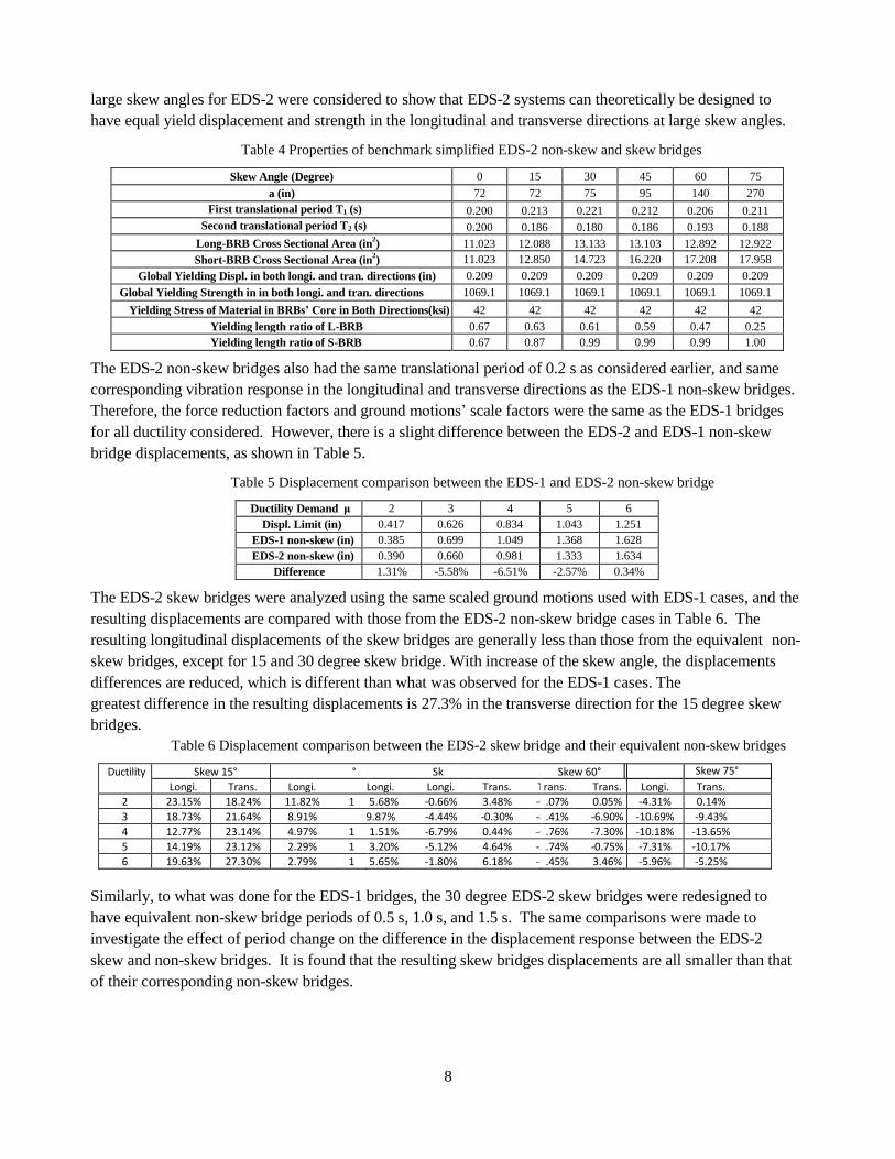
large skew angles for EDS-2 were considered to show that EDS-2 systems can theoretically be designed to

have equal yield displacement and strength in the longitudinal and transverse directions at large skew angles.

Table 4 Properties of benchmark simplified EDS-2 non-skew and skew bridges

Skew Angle (Degree) 0 15 30 45 60 75

a (in) 72 72 75 95 140 270

First translational period T1 (s) 0.200 0.213 0.221 0.212 0.206 0.211

Second translational period T2 (s) 0.200 0.186 0.180 0.186 0.193 0.188

Long-BRB Cross Sectional Area (in2) 11.023 12.088 13.133 13.103 12.892 12.922

Short-BRB Cross Sectional Area (in2) 11.023 12.850 14.723 16.220 17.208 17.958

Global Yielding Displ. in both longi. and tran. directions (in) 0.209 0.209 0.209 0.209 0.209 0.209

Global Yielding Strength in in both longi. and tran. directions

(kips)

1069.1 1069.1 1069.1 1069.1 1069.1 1069.1

Yielding Stress of Material in BRBs’ Core in Both Directions(ksi) 42 42 42 42 42 42

Yielding length ratio of L-BRB 0.67 0.63 0.61 0.59 0.47 0.25

Yielding length ratio of S-BRB 0.67 0.87 0.99 0.99 0.99 1.00

The EDS-2 non-skew bridges also had the same translational period of 0.2 s as considered earlier, and same

corresponding vibration response in the longitudinal and transverse directions as the EDS-1 non-skew bridges.

Therefore, the force reduction factors and ground motions’ scale factors were the same as the EDS-1 bridges

for all ductility considered. However, there is a slight difference between the EDS-2 and EDS-1 non-skew

bridge displacements, as shown in Table 5.

Table 5 Displacement comparison between the EDS-1 and EDS-2 non-skew bridge

Ductility Demand μ 2 3 4 5 6

Displ. Limit (in) 0.417 0.626 0.834 1.043 1.251

EDS-1 non-skew (in) 0.385 0.699 1.049 1.368 1.628

EDS-2 non-skew (in) 0.390 0.660 0.981 1.333 1.634

Difference 1.31% -5.58% -6.51% -2.57% 0.34%

The EDS-2 skew bridges were analyzed using the same scaled ground motions used with EDS-1 cases, and the

resulting displacements are compared with those from the EDS-2 non-skew bridge cases in Table 6. The

resulting longitudinal displacements of the skew bridges are generally less than those from the equivalent non-

skew bridges, except for 15 and 30 degree skew bridge. With increase of the skew angle, the displacements

differences are reduced, which is different than what was observed for the EDS-1 cases. The

greatest difference in the resulting displacements is 27.3% in the transverse direction for the 15 degree skew

bridges.

Table 6 Displacement comparison between the EDS-2 skew bridge and their equivalent non-skew bridges

Skew 75°

Similarly, to what was done for the EDS-1 bridges, the 30 degree EDS-2 skew bridges were redesigned to

have equivalent non-skew bridge periods of 0.5 s, 1.0 s, and 1.5 s. The same comparisons were made to

investigate the effect of period change on the difference in the displacement response between the EDS-2

skew and non-skew bridges. It is found that the resulting skew bridges displacements are all smaller than that

of their corresponding non-skew bridges.

Ductility Skew 15° ° Sk Skew 60° Longi. Trans. Longi. Longi. Longi. Trans. T rans. Trans. Longi. Trans.

2 23.15% 18.24% 11.82% 1 5.68% -0.66% 3.48% -6 .07% 0.05% -4.31% 0.14%

3 18.73% 21.64% 8.91% 9.87% -4.44% -0.30% -8 .41% -6.90% -10.69% -9.43%

4 12.77% 23.14% 4.97% 1 1.51% -6.79% 0.44% -6 .76% -7.30% -10.18% -13.65%

5 14.19% 23.12% 2.29% 1 3.20% -5.12% 4.64% -3 .74% -0.75% -7.31% -10.17%

6 19.63% 27.30% 2.79% 1 5.65% -1.80% 6.18% -1 .45% 3.46% -5.96% -5.25%

9

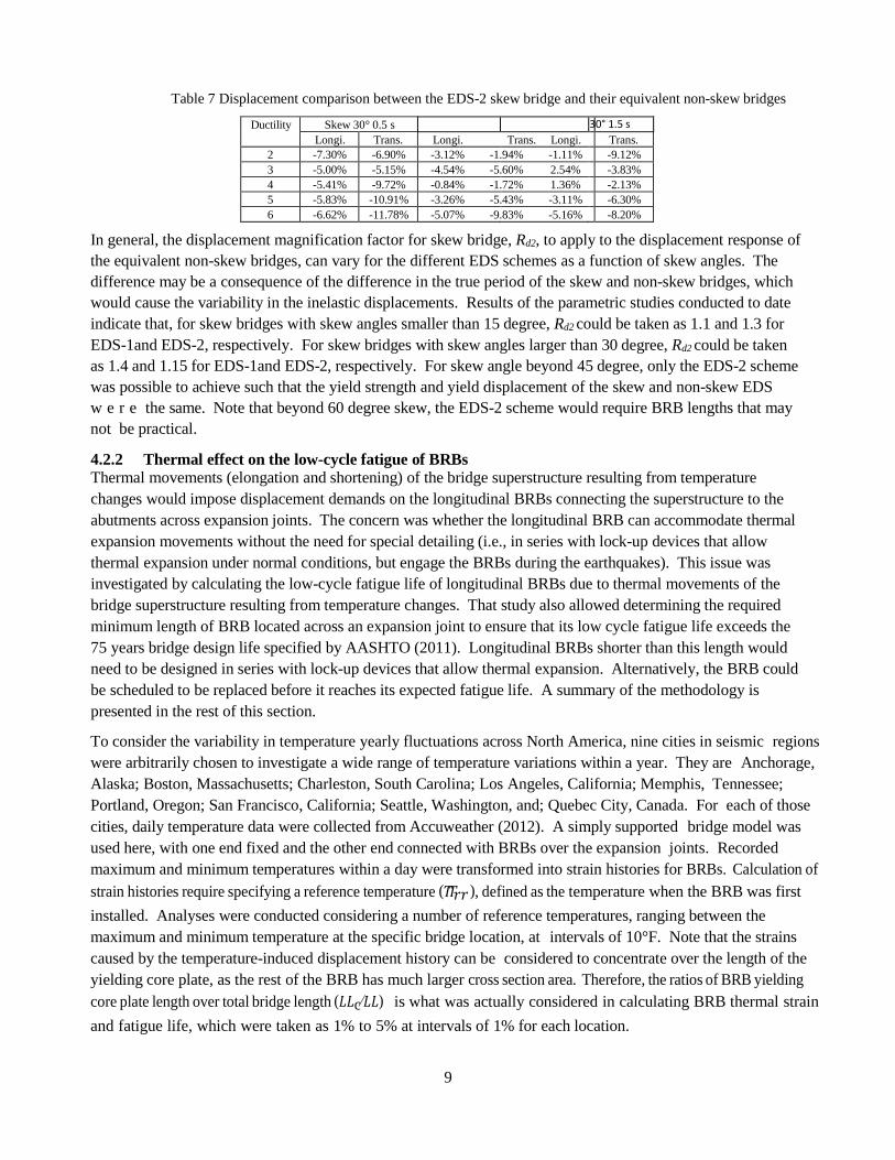
Table 7 Displacement comparison between the EDS-2 skew bridge and their equivalent non-skew bridges

30° 1.5 s

In general, the displacement magnification factor for skew bridge, Rd2, to apply to the displacement response of

the equivalent non-skew bridges, can vary for the different EDS schemes as a function of skew angles. The

difference may be a consequence of the difference in the true period of the skew and non-skew bridges, which

would cause the variability in the inelastic displacements. Results of the parametric studies conducted to date

indicate that, for skew bridges with skew angles smaller than 15 degree, Rd2 could be taken as 1.1 and 1.3 for

EDS-1and EDS-2, respectively. For skew bridges with skew angles larger than 30 degree, Rd2 could be taken

as 1.4 and 1.15 for EDS-1and EDS-2, respectively. For skew angle beyond 45 degree, only the EDS-2 scheme

was possible to achieve such that the yield strength and yield displacement of the skew and non-skew EDS

w e r e the same. Note that beyond 60 degree skew, the EDS-2 scheme would require BRB lengths that may

not be practical.

4.2.2 Thermal effect on the low-cycle fatigue of BRBs Thermal movements (elongation and shortening) of the bridge superstructure resulting from temperature

changes would impose displacement demands on the longitudinal BRBs connecting the superstructure to the

abutments across expansion joints. The concern was whether the longitudinal BRB can accommodate thermal

expansion movements without the need for special detailing (i.e., in series with lock-up devices that allow

thermal expansion under normal conditions, but engage the BRBs during the earthquakes). This issue was

investigated by calculating the low-cycle fatigue life of longitudinal BRBs due to thermal movements of the

bridge superstructure resulting from temperature changes. That study also allowed determining the required

minimum length of BRB located across an expansion joint to ensure that its low cycle fatigue life exceeds the

75 years bridge design life specified by AASHTO (2011). Longitudinal BRBs shorter than this length would

need to be designed in series with lock-up devices that allow thermal expansion. Alternatively, the BRB could

be scheduled to be replaced before it reaches its expected fatigue life. A summary of the methodology is

presented in the rest of this section.

To consider the variability in temperature yearly fluctuations across North America, nine cities in seismic regions

were arbitrarily chosen to investigate a wide range of temperature variations within a year. They are Anchorage,

Alaska; Boston, Massachusetts; Charleston, South Carolina; Los Angeles, California; Memphis, Tennessee;

Portland, Oregon; San Francisco, California; Seattle, Washington, and; Quebec City, Canada. For each of those

cities, daily temperature data were collected from Accuweather (2012). A simply supported bridge model was

used here, with one end fixed and the other end connected with BRBs over the expansion joints. Recorded

maximum and minimum temperatures within a day were transformed into strain histories for BRBs. Calculation of

strain histories require specifying a reference temperature (𝑇𝑇𝑟𝑟 ), defined as the temperature when the BRB was first

installed. Analyses were conducted considering a number of reference temperatures, ranging between the

maximum and minimum temperature at the specific bridge location, at intervals of 10°F. Note that the strains

caused by the temperature-induced displacement history can be considered to concentrate over the length of the

yielding core plate, as the rest of the BRB has much larger cross section area. Therefore, the ratios of BRB yielding

core plate length over total bridge length (𝐿𝐿c⁄𝐿𝐿) is what was actually considered in calculating BRB thermal strain

and fatigue life, which were taken as 1% to 5% at intervals of 1% for each location.

Ductility Skew 30° 0.5 s Longi. Trans. Longi.

T

r

Trans. Longi. Trans.

2 -7.30% -6.90% -3.12% -1 .94% -1.11% -9.12%

3 -5.00% -5.15% -4.54% -5 .60% 2.54% -3.83%

4 -5.41% -9.72% -0.84% -1 .72% 1.36% -2.13%

5 -5.83% -10.91% -3.26% -5 .43% -3.11% -6.30%

6 -6.62% -11.78% -5.07% -9 .83% -5.16% -8.20%

10

The software program Fatiga Version 1.03 was chosen to calculate low-cycle fatigue life using the strain

history and the fatigue properties of the BRB’s core plate material (ASTM A36 steel material). The resulting

strain histories were characterized as variable amplitude strain loading (because the amplitude of the strain

ranges changed in each cycle instead of being of constant amplitude). Strain cycles were obtained using the

Rainflow Counting method and the damage (i.e. the percentage of the total fatigue life) caused by cycles at

each stress-range amplitude were accumulated using Miner’s rule. The Smith-Watson and Topper (1970)

method was used to calculate fatigue life, considering the tensile mean stress effect. The damage done by all

cycles in the temperature-induced strain history (i.e., for one year) can be obtained. Since the BRB fails when

the cumulative damage reaches 1.0, therefore, the fatigue life is the reciprocal of the damage caused by the

strain history for one year (i.e., a single application of the temperature-induced strain history). In other words,

the fatigue life is the number of times that this strain history can be applied to the BRB before it fails.

In places where the yearly fluctuations of temperature were more severe (the most severe case being Memphis

for all cities considered), the calculated fatigue life of the BRB was less compared to places where the yearly

temperature variations were smaller. In general, a minimum length ratio of the BRB’s yielding core plate of 3%

proved to be sufficient to avoid low-cycle fatigue of the BRB due to 75 years of thermal changes on the bridge

superstructure for all locations, for all the install temperatures and cities considered.

Note that, in this low-cycle fatigue study, the longitudinal BRB was considered to be installed horizontally

aligned with the bridge’s longitudinal axis. However, in both the EDS-1 and EDS-2 schemes, BRBs are

installed at an angle with the bridge longitudinal axis, both vertically and horizontal. Considering this

geometry effect would result in smaller minimum length demands for the BRBs to satisfy their low-cycle

fatigue performance requirement. As a result, the recommended minimum yielding core plate length ratio of

BRB of 3% is conservative and was kept for simplicity.

However, the above estimated fatigue life of BRBs obtained from Fatiga is solely based on the axial strain

loading applied to its core steel (for ASTM A36 material). Note that the core plate of a BRB typically

develops local buckling under the applied low-cycle strain loading (albeit of constrained amplitude). This

local buckling produces additional flexural plastic deformations that add up to the pure axial strains.

Therefore, a calibration factor was deemed necessary to account for the fact that the local buckling of BRBs

may reduce the estimated low-cycle fatigue life results obtained based on metal properties.

Since little data is available for the low-cycle fatigue of BRBs under variable amplitude loading, prior to the

tests conducted for this project, a tentative calibration factor was contemplated based on the constant

amplitude loading experiments by Usami et al.(2011), Wang et al.(2012), Akira et al. (2000) and Maeda et.

al. (1998). The strain history applied to the BRBs up to failure in those tests was input to Fatiga to get the

estimated fatigue life of each tested BRB. The damage calculated by Fatiga for each of these tests to failure is

essentially equal to the calibration factor. Based on those results, the calibration factor was found to vary with

the strain magnitude, ranging from 0.05 to 0.53. Note that this calibration factor is also expected to depend on

how the BRB is fabricated, as this would have an impact on the amplitude of the local buckling in the BRB

core. Therefore, the minimum BRB’s yielding core plate length ratio that is sufficient to avoid low-cycle

fatigue of the BRB for 75 years of thermal changes on the bridge superstructure could be larger than 3%.

4.3 Stage 2-Experimental Investigation

Quasi-static tests were performed on two types of BRBs using a shake table to apply displacement histories, to

determine their ultimate inelastic cyclic performance when subjected to different scenarios of individual or

sequential displacement protocols. In this section, these experimental results are presented and the

performance of each type of BRB is examined. Section 4.3.1 presents the design of the test set-up and the two

11

types of BRB specimens, together with a description of their different behaviors expected during the tests. A

description of instrumentation of the BRB specimens is provided in Section 4.3.2. The initial test protocols

that were intended to be applied to the BRB are described in Section 4.3.3, including the bidirectional and

temperature-induced axial displacement histories. Section 4.3.4 presents the detailed adjusted test protocols

for specific BRB and the resulting hysteretic behaviors of each BRB under different displacement histories.

Section 4.3.5 summarizes and compares the inelastic cumulative displacements and fatigue damage of each

tested BRB.

4.3.1 Test set-up and BRB specimens

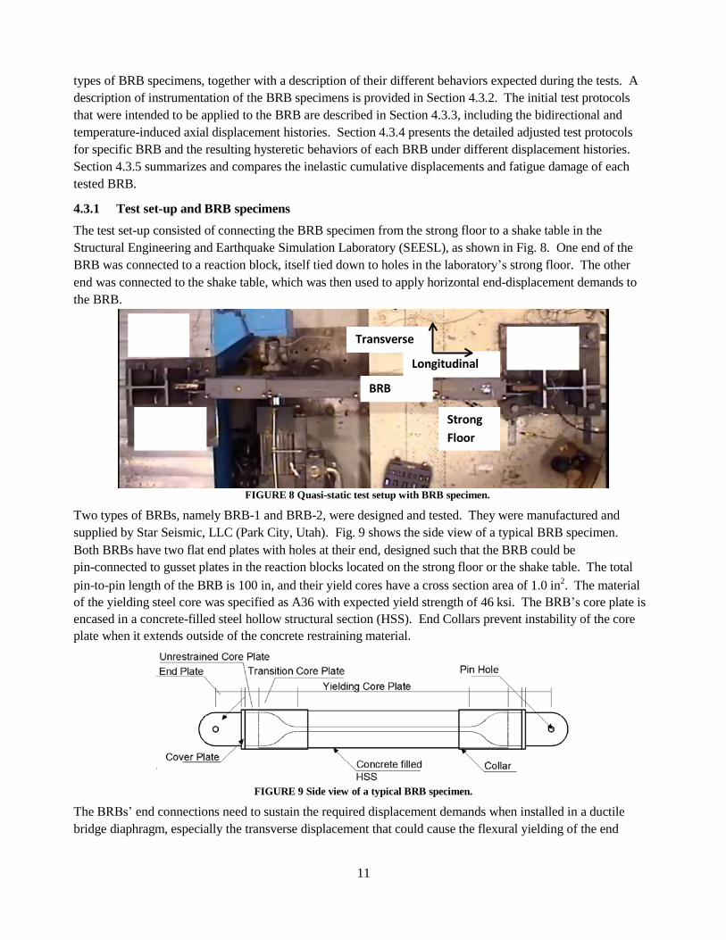
The test set-up consisted of connecting the BRB specimen from the strong floor to a shake table in the

Structural Engineering and Earthquake Simulation Laboratory (SEESL), as shown in Fig. 8. One end of the

BRB was connected to a reaction block, itself tied down to holes in the laboratory’s strong floor. The other

end was connected to the shake table, which was then used to apply horizontal end-displacement demands to

the BRB.

FIGURE 8 Quasi-static test setup with BRB specimen.

Two types of BRBs, namely BRB-1 and BRB-2, were designed and tested. They were manufactured and

supplied by Star Seismic, LLC (Park City, Utah). Fig. 9 shows the side view of a typical BRB specimen.

Both BRBs have two flat end plates with holes at their end, designed such that the BRB could be

pin-connected to gusset plates in the reaction blocks located on the strong floor or the shake table. The total

pin-to-pin length of the BRB is 100 in, and their yield cores have a cross section area of 1.0 in2. The material

of the yielding steel core was specified as A36 with expected yield strength of 46 ksi. The BRB’s core plate is

encased in a concrete-filled steel hollow structural section (HSS). End Collars prevent instability of the core

plate when it extends outside of the concrete restraining material.

FIGURE 9 Side view of a typical BRB specimen.

The BRBs’ end connections need to sustain the required displacement demands when installed in a ductile

bridge diaphragm, especially the transverse displacement that could cause the flexural yielding of the end

Transverse

Longitudinal

BRB

Strong

Floor

12

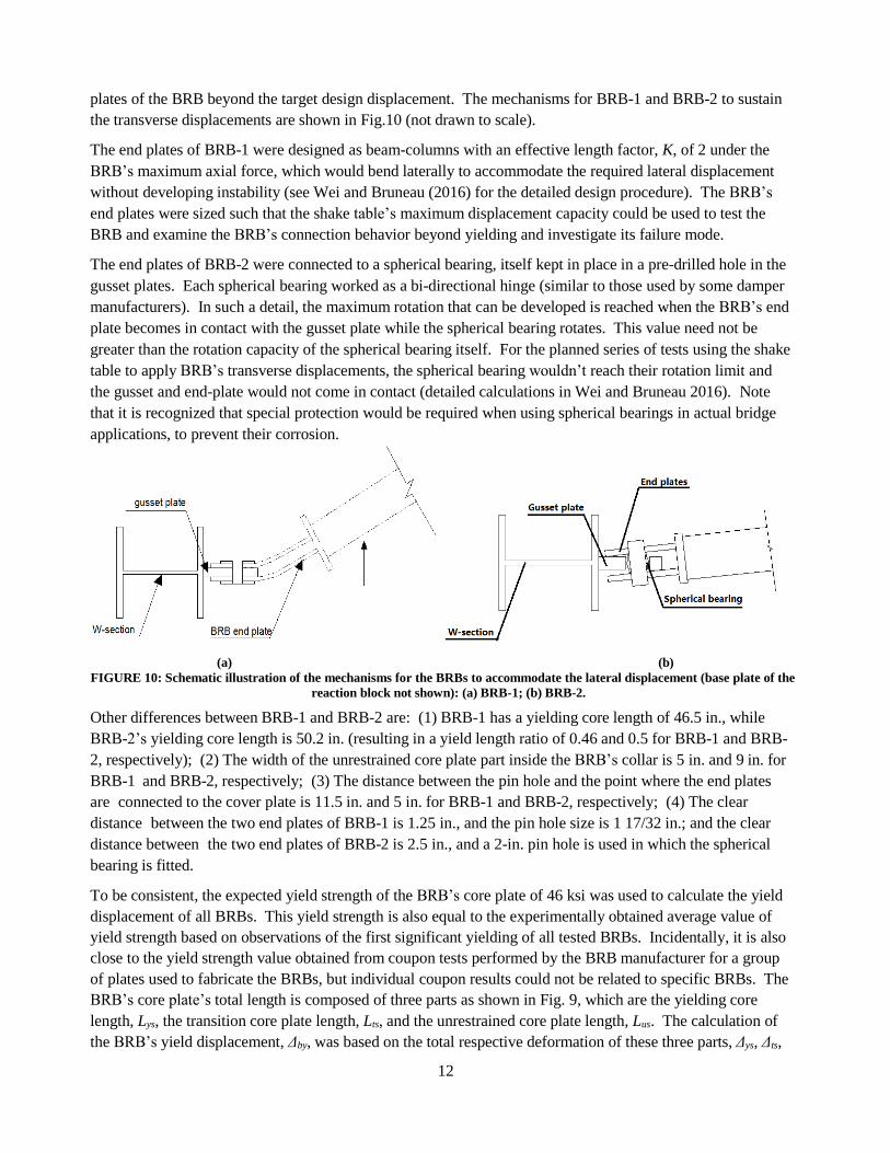
plates of the BRB beyond the target design displacement. The mechanisms for BRB-1 and BRB-2 to sustain

the transverse displacements are shown in Fig.10 (not drawn to scale).

The end plates of BRB-1 were designed as beam-columns with an effective length factor, K, of 2 under the

BRB’s maximum axial force, which would bend laterally to accommodate the required lateral displacement

without developing instability (see Wei and Bruneau (2016) for the detailed design procedure). The BRB’s

end plates were sized such that the shake table’s maximum displacement capacity could be used to test the

BRB and examine the BRB’s connection behavior beyond yielding and investigate its failure mode.

The end plates of BRB-2 were connected to a spherical bearing, itself kept in place in a pre-drilled hole in the

gusset plates. Each spherical bearing worked as a bi-directional hinge (similar to those used by some damper

manufacturers). In such a detail, the maximum rotation that can be developed is reached when the BRB’s end

plate becomes in contact with the gusset plate while the spherical bearing rotates. This value need not be

greater than the rotation capacity of the spherical bearing itself. For the planned series of tests using the shake

table to apply BRB’s transverse displacements, the spherical bearing wouldn’t reach their rotation limit and

the gusset and end-plate would not come in contact (detailed calculations in Wei and Bruneau 2016). Note

that it is recognized that special protection would be required when using spherical bearings in actual bridge

applications, to prevent their corrosion.

(a) (b)

FIGURE 10: Schematic illustration of the mechanisms for the BRBs to accommodate the lateral displacement (base plate of the

reaction block not shown): (a) BRB-1; (b) BRB-2.

Other differences between BRB-1 and BRB-2 are: (1) BRB-1 has a yielding core length of 46.5 in., while

BRB-2’s yielding core length is 50.2 in. (resulting in a yield length ratio of 0.46 and 0.5 for BRB-1 and BRB-

2, respectively); (2) The width of the unrestrained core plate part inside the BRB’s collar is 5 in. and 9 in. for

BRB-1 and BRB-2, respectively; (3) The distance between the pin hole and the point where the end plates

are connected to the cover plate is 11.5 in. and 5 in. for BRB-1 and BRB-2, respectively; (4) The clear

distance between the two end plates of BRB-1 is 1.25 in., and the pin hole size is 1 17/32 in.; and the clear

distance between the two end plates of BRB-2 is 2.5 in., and a 2-in. pin hole is used in which the spherical

bearing is fitted.

To be consistent, the expected yield strength of the BRB’s core plate of 46 ksi was used to calculate the yield

displacement of all BRBs. This yield strength is also equal to the experimentally obtained average value of

yield strength based on observations of the first significant yielding of all tested BRBs. Incidentally, it is also

close to the yield strength value obtained from coupon tests performed by the BRB manufacturer for a group

of plates used to fabricate the BRBs, but individual coupon results could not be related to specific BRBs. The

BRB’s core plate’s total length is composed of three parts as shown in Fig. 9, which are the yielding core

length, Lys, the transition core plate length, Lts, and the unrestrained core plate length, Lus. The calculation of

the BRB’s yield displacement, Δby, was based on the total respective deformation of these three parts, Δys, Δts,

13

Δus, as expressed by Equation 3.

𝛥𝛥𝑏𝑏𝑏𝑏 = 𝛥𝛥𝑏𝑏𝑦𝑦 + 𝛥𝛥𝑡𝑡𝑦𝑦 + 𝛥𝛥𝑢𝑢𝑦𝑦 (3)

The corresponding calculated yield displacement Δby of BRB-1 and BRB-2 is 0.107 in. and 0.081,” respectively.

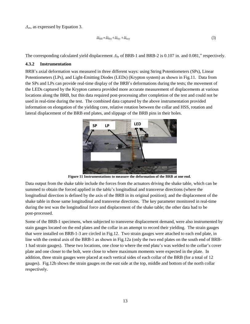
4.3.2 Instrumentation

BRB’s axial deformation was measured in three different ways: using String Potentiometers (SPs), Linear

Potentiometers (LPs), and Light-Emitting Diodes (LEDs) (Krypton system) as shown in Fig.11. Data from

the SPs and LPs can provide real-time display of the BRB’s deformations during the tests; the movement of

the LEDs captured by the Krypton camera provided more accurate measurement of displacements at various

locations along the BRB, but this data required post-processing after completion of the test and could not be

used in real-time during the test. The combined data captured by the above instrumentation provided

information on elongation of the yielding core, relative rotation between the collar and HSS, rotation and

lateral displacement of the BRB end plates, and slippage of the BRB pins in their holes.

Figure 11 Instrumentations to measure the deformation of the BRB at one end.

Data output from the shake table include the forces from the actuators driving the shake table, which can be

summed to obtain the forced applied in the table’s longitudinal and transverse directions (where the

longitudinal direction is defined by the axis of the BRB in its original position); and the displacement of the

shake table in those same longitudinal and transverse directions. The key parameter monitored in real-time

during the test was the longitudinal force and displacement of the shake table; the other data had to be

post-processed.

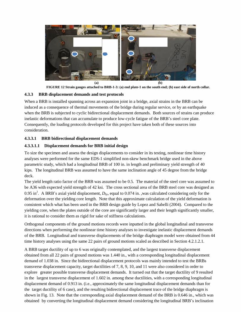
Some of the BRB-1 specimens, when subjected to transverse displacement demand, were also instrumented by

stain gauges located on the end plates and the collar in an attempt to record their yielding. The strain gauges

that were installed on BRB-1-3 are circled in Fig.12. Two strain gauges were attached to each end plate, in

line with the central axis of the BRB-1 as shown in Fig.12a (only the two end plates on the south end of BRB-

1 had strain gauges). These two locations, one close to where the end plate’s was welded to the collar’s cover

plate and one closer to the bolt, were close to where maximum moments were expected in the plate. In

addition, three strain gauges were placed at each vertical sides of each collar of the BRB (for a total of 12

gauges). Fig.12b shows the strain gauges on the east side at the top, middle and bottom of the north collar

respectively.

SP LP LED

(a) (b)

FIGURE 12 Strain gauges attached to BRB-1-3: (a) end plate-1 on the south end; (b) east side of north collar.

4.3.3 BRB displacement demands and test protocols

When a BRB is installed spanning across an expansion joint in a bridge, axial strains in the BRB can be

induced as a consequence of thermal movements of the bridge during regular service, or by an earthquake

when the BRB is subjected to cyclic bidirectional displacement demands. Both sources of strains can produce

inelastic deformations that can accumulate to produce low-cycle fatigue of the BRB’s steel core plate.

Consequently, the loading protocols developed for this project have taken both of these sources into

consideration.

4.3.3.1 BRB bidirectional displacement demands

4.3.3.1.1 Displacement demands for BRB initial design

To size the specimen and assess the design displacements to consider in its testing, nonlinear time history

analyses were performed for the same EDS-1 simplified non-skew benchmark bridge used in the above

parametric study, which had a longitudinal BRB of 100 in. in length and preliminary yield strength of 40

kips. The longitudinal BRB was assumed to have the same inclination angle of 45 degree from the bridge

deck.

The yield length ratio factor of the BRB was assumed to be 0.5. The material of the steel core was assumed to

be A36 with expected yield strength of 42 ksi. The cross sectional area of the BRB steel core was designed as

0.95 in2. A BRB’s axial yield displacement, Dby, equal to 0.074 in. ,was calculated considering only for the

deformation over the yielding core length. Note that this approximate calculation of the yield deformation is

consistent which what has been used in the BRB design guide by Lopez and Sabelli (2004). Compared to the

yielding core, when the plates outside of the core are significantly larger and their length significantly smaller,

it is rational to consider them as rigid for sake of stiffness calculations.

Orthogonal components of the ground motions records were inputted in the global longitudinal and transverse

directions when performing the nonlinear time history analyses to investigate inelastic displacement demands

of the BRB. Longitudinal and transverse displacements of the bridge diaphragm model were obtained from 44

time history analyses using the same 22 pairs of ground motions scaled as described in Section 4.2.1.2.1.

A BRB target ductility of up to 6 was originally contemplated, and the largest transverse displacement

obtained from all 22 pairs of ground motions was 1.440 in., with a corresponding longitudinal displacement

demand of 1.038 in. Since the bidirectional displacement protocols was mainly intended to test the BRBs

transverse displacement capacity, target ductilities of 7, 8, 9, 10, and 11 were also considered in order to

explore greater possible transverse displacement demands. It turned out that the target ductility of 9 resulted

in the largest transverse displacement of 1.602 in. among these ductilities, with a corresponding longitudinal

displacement demand of 0.913 in. (i.e., approximately the same longitudinal displacement demands than for

the target ductility of 6 case), and the resulting bidirectional displacement trace of the bridge diaphragm is

shown in Fig. 13. Note that the corresponding axial displacement demand of the BRB is 0.646 in., which was

obtained by converting the longitudinal displacement demand considering the longitudinal BRB’s inclination

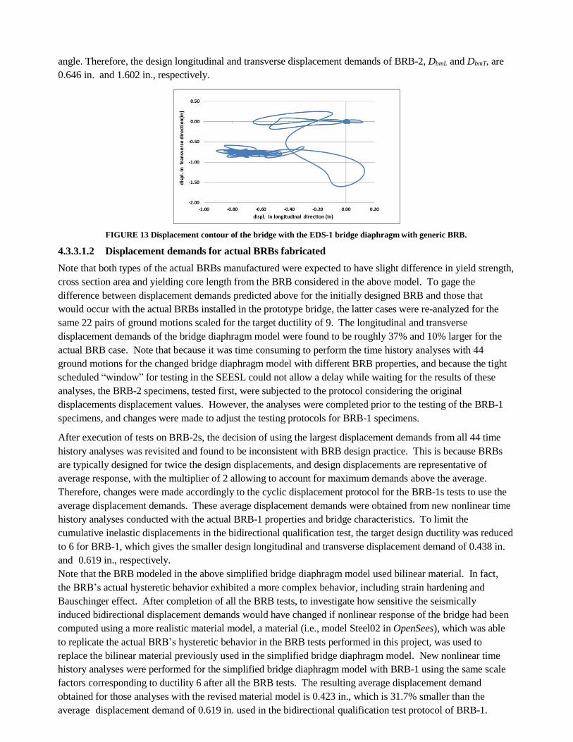
angle. Therefore, the design longitudinal and transverse displacement demands of BRB-2, DbmL and DbmT, are

0.646 in. and 1.602 in., respectively.

FIGURE 13 Displacement contour of the bridge with the EDS-1 bridge diaphragm with generic BRB.

4.3.3.1.2 Displacement demands for actual BRBs fabricated

Note that both types of the actual BRBs manufactured were expected to have slight difference in yield strength,

cross section area and yielding core length from the BRB considered in the above model. To gage the

difference between displacement demands predicted above for the initially designed BRB and those that

would occur with the actual BRBs installed in the prototype bridge, the latter cases were re-analyzed for the

same 22 pairs of ground motions scaled for the target ductility of 9. The longitudinal and transverse

displacement demands of the bridge diaphragm model were found to be roughly 37% and 10% larger for the

actual BRB case. Note that because it was time consuming to perform the time history analyses with 44

ground motions for the changed bridge diaphragm model with different BRB properties, and because the tight

scheduled “window” for testing in the SEESL could not allow a delay while waiting for the results of these

analyses, the BRB-2 specimens, tested first, were subjected to the protocol considering the original

displacements displacement values. However, the analyses were completed prior to the testing of the BRB-1

specimens, and changes were made to adjust the testing protocols for BRB-1 specimens.

After execution of tests on BRB-2s, the decision of using the largest displacement demands from all 44 time

history analyses was revisited and found to be inconsistent with BRB design practice. This is because BRBs

are typically designed for twice the design displacements, and design displacements are representative of

average response, with the multiplier of 2 allowing to account for maximum demands above the average.

Therefore, changes were made accordingly to the cyclic displacement protocol for the BRB-1s tests to use the

average displacement demands. These average displacement demands were obtained from new nonlinear time

history analyses conducted with the actual BRB-1 properties and bridge characteristics. To limit the

cumulative inelastic displacements in the bidirectional qualification test, the target design ductility was reduced

to 6 for BRB-1, which gives the smaller design longitudinal and transverse displacement demand of 0.438 in.

and 0.619 in., respectively.

Note that the BRB modeled in the above simplified bridge diaphragm model used bilinear material. In fact,

the BRB’s actual hysteretic behavior exhibited a more complex behavior, including strain hardening and

Bauschinger effect. After completion of all the BRB tests, to investigate how sensitive the seismically

induced bidirectional displacement demands would have changed if nonlinear response of the bridge had been

computed using a more realistic material model, a material (i.e., model Steel02 in OpenSees), which was able

to replicate the actual BRB’s hysteretic behavior in the BRB tests performed in this project, was used to

replace the bilinear material previously used in the simplified bridge diaphragm model. New nonlinear time

history analyses were performed for the simplified bridge diaphragm model with BRB-1 using the same scale

factors corresponding to ductility 6 after all the BRB tests. The resulting average displacement demand

obtained for those analyses with the revised material model is 0.423 in., which is 31.7% smaller than the

average displacement demand of 0.619 in. used in the bidirectional qualification test protocol of BRB-1.

Therefore, it is found that it was conservative to use the larger displacement demands to test the BRB.

4.3.3.2 BRB bidirectional qualification test protocols

The standard test protocol used for the qualification test of BRBs is outlined in details in the AISC 341-10

Specifications as follows: first apply 2 cycles of loading at the deformation corresponding to each of 1.0Dby,

0.5DbmL, 1.0DbmL, 1.5DbmL and 2.0DbmL; then apply additional cycles of loading at the deformation

corresponding to 1.5DbmL as required for the BRB test specimen to achieve a cumulative inelastic axial

deformations of at least 200 times the yield displacement. This protocol was developed for BRBs (tested

alone and in sub-assemblies) principally subjected to axial displacements. Given that in the current proposed

application in bidirectional diaphragms, BRBs are explicitly expected to be subjected to significant

out-of-plane deformations in addition to axial ones, the existing test protocol had to be adapted.

The design objectives adopted here was that the BRB’s end plates (for BRB-1) must not yield due to

out-of-plane bending before the transverse design displacement DbmT is reached. Furthermore, AISC specifies

that the BRB’s core plate must sustain progressively increasing axial displacements until a value equal to

twice the design displacement; it was therefore extrapolated here that the BRB should also not fail at the twice

the displacement demands in both directions during the bidirectional qualification test. Therefore, the

bidirectional BRB test was conducted by controlling the level of axial (longitudinal) and transverse

deformations imposed on the BRB at each displacement demand level. Bi-directionality was introduced in the

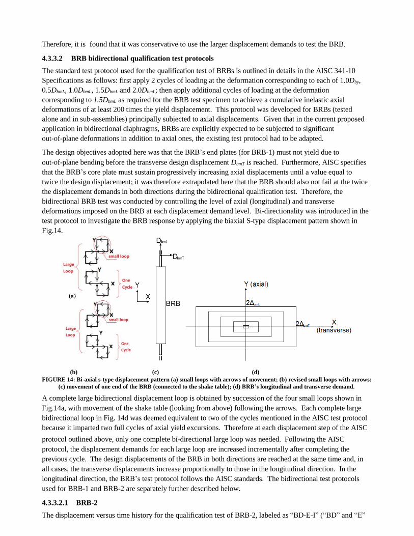
test protocol to investigate the BRB response by applying the biaxial S-type displacement pattern shown in

Fig.14.

(b) (c) (d)

FIGURE 14: Bi-axial s-type displacement pattern (a) small loops with arrows of movement; (b) revised small loops with arrows;

(c) movement of one end of the BRB (connected to the shake table); (d) BRB’s longitudinal and transverse demand.

A complete large bidirectional displacement loop is obtained by succession of the four small loops shown in

Fig.14a, with movement of the shake table (looking from above) following the arrows. Each complete large

bidirectional loop in Fig. 14d was deemed equivalent to two of the cycles mentioned in the AISC test protocol

because it imparted two full cycles of axial yield excursions. Therefore at each displacement step of the AISC

protocol outlined above, only one complete bi-directional large loop was needed. Following the AISC

protocol, the displacement demands for each large loop are increased incrementally after completing the

previous cycle. The design displacements of the BRB in both directions are reached at the same time and, in

all cases, the transverse displacements increase proportionally to those in the longitudinal direction. In the

longitudinal direction, the BRB’s test protocol follows the AISC standards. The bidirectional test protocols

used for BRB-1 and BRB-2 are separately further described below.

4.3.3.2.1 BRB-2

The displacement versus time history for the qualification test of BRB-2, labeled as “BD-E-I” (“BD” and “E”

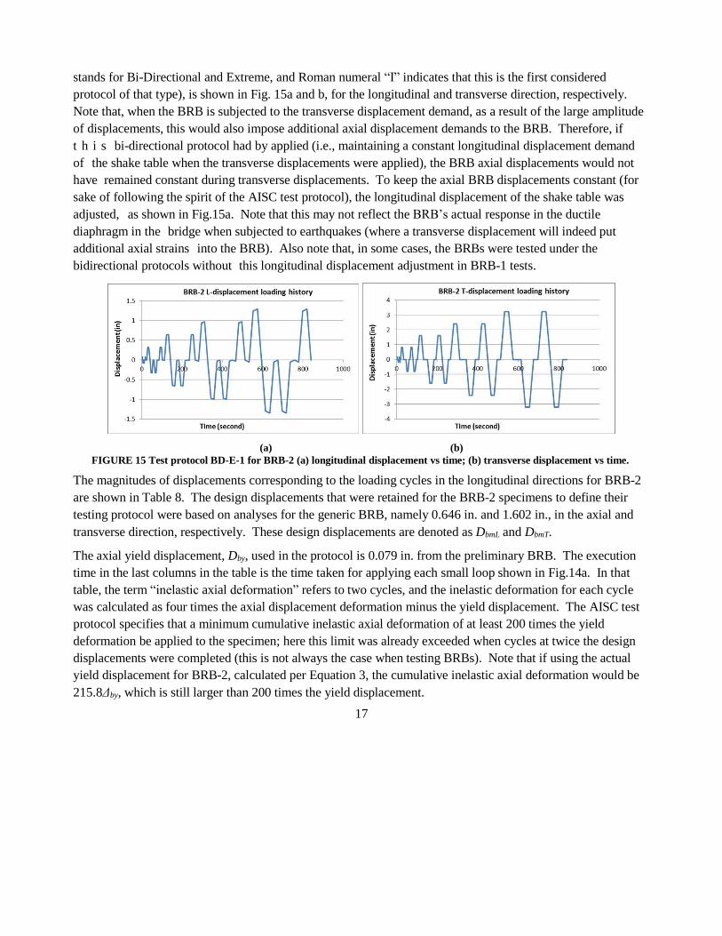
stands for Bi-Directional and Extreme, and Roman numeral “I” indicates that this is the first considered

protocol of that type), is shown in Fig. 15a and b, for the longitudinal and transverse direction, respectively.

Note that, when the BRB is subjected to the transverse displacement demand, as a result of the large amplitude

of displacements, this would also impose additional axial displacement demands to the BRB. Therefore, if

t h i s bi-directional protocol had by applied (i.e., maintaining a constant longitudinal displacement demand

of the shake table when the transverse displacements were applied), the BRB axial displacements would not

have remained constant during transverse displacements. To keep the axial BRB displacements constant (for

sake of following the spirit of the AISC test protocol), the longitudinal displacement of the shake table was

adjusted, as shown in Fig.15a. Note that this may not reflect the BRB’s actual response in the ductile

diaphragm in the bridge when subjected to earthquakes (where a transverse displacement will indeed put

additional axial strains into the BRB). Also note that, in some cases, the BRBs were tested under the

bidirectional protocols without this longitudinal displacement adjustment in BRB-1 tests.

(a) (b)

FIGURE 15 Test protocol BD-E-1 for BRB-2 (a) longitudinal displacement vs time; (b) transverse displacement vs time.

The magnitudes of displacements corresponding to the loading cycles in the longitudinal directions for BRB-2

are shown in Table 8. The design displacements that were retained for the BRB-2 specimens to define their

testing protocol were based on analyses for the generic BRB, namely 0.646 in. and 1.602 in., in the axial and

transverse direction, respectively. These design displacements are denoted as DbmL and DbmT.

The axial yield displacement, Dby, used in the protocol is 0.079 in. from the preliminary BRB. The execution

time in the last columns in the table is the time taken for applying each small loop shown in Fig.14a. In that

table, the term “inelastic axial deformation” refers to two cycles, and the inelastic deformation for each cycle

was calculated as four times the axial displacement deformation minus the yield displacement. The AISC test

protocol specifies that a minimum cumulative inelastic axial deformation of at least 200 times the yield

deformation be applied to the specimen; here this limit was already exceeded when cycles at twice the design

displacements were completed (this is not always the case when testing BRBs). Note that if using the actual

yield displacement for BRB-2, calculated per Equation 3, the cumulative inelastic axial deformation would be

215.8Δby, which is still larger than 200 times the yield displacement.

17

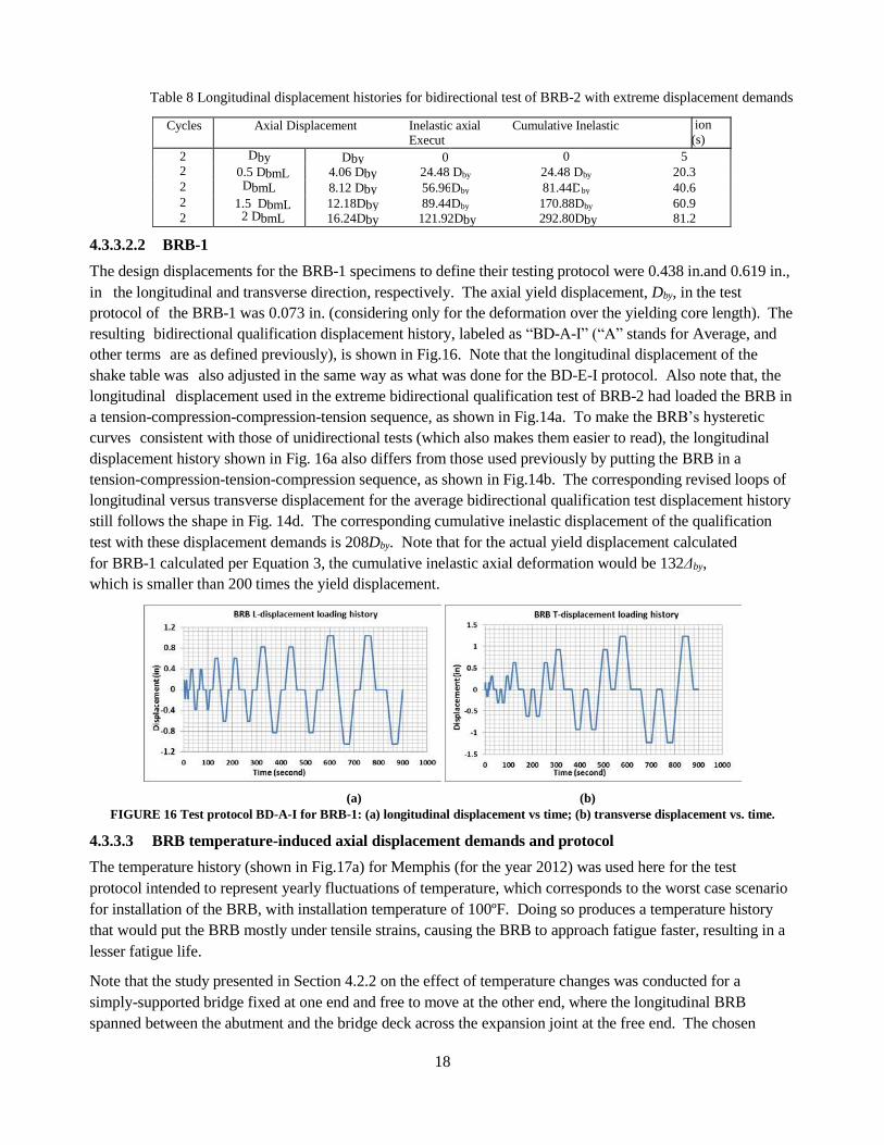
Table 8 Longitudinal displacement histories for bidirectional test of BRB-2 with extreme displacement demands

ion

(s)

4.3.3.2.2 BRB-1

The design displacements for the BRB-1 specimens to define their testing protocol were 0.438 in.and 0.619 in.,

in the longitudinal and transverse direction, respectively. The axial yield displacement, Dby, in the test

protocol of the BRB-1 was 0.073 in. (considering only for the deformation over the yielding core length). The

resulting bidirectional qualification displacement history, labeled as “BD-A-I” (“A” stands for Average, and

other terms are as defined previously), is shown in Fig.16. Note that the longitudinal displacement of the

shake table was also adjusted in the same way as what was done for the BD-E-I protocol. Also note that, the

longitudinal displacement used in the extreme bidirectional qualification test of BRB-2 had loaded the BRB in

a tension-compression-compression-tension sequence, as shown in Fig.14a. To make the BRB’s hysteretic

curves consistent with those of unidirectional tests (which also makes them easier to read), the longitudinal

displacement history shown in Fig. 16a also differs from those used previously by putting the BRB in a

tension-compression-tension-compression sequence, as shown in Fig.14b. The corresponding revised loops of

longitudinal versus transverse displacement for the average bidirectional qualification test displacement history

still follows the shape in Fig. 14d. The corresponding cumulative inelastic displacement of the qualification

test with these displacement demands is 208Dby. Note that for the actual yield displacement calculated

for BRB-1 calculated per Equation 3, the cumulative inelastic axial deformation would be 132Δby,

which is smaller than 200 times the yield displacement.

(a) (b)

FIGURE 16 Test protocol BD-A-I for BRB-1: (a) longitudinal displacement vs time; (b) transverse displacement vs. time.

4.3.3.3 BRB temperature-induced axial displacement demands and protocol

The temperature history (shown in Fig.17a) for Memphis (for the year 2012) was used here for the test

protocol intended to represent yearly fluctuations of temperature, which corresponds to the worst case scenario

for installation of the BRB, with installation temperature of 100ºF. Doing so produces a temperature history

that would put the BRB mostly under tensile strains, causing the BRB to approach fatigue faster, resulting in a

lesser fatigue life.

Note that the study presented in Section 4.2.2 on the effect of temperature changes was conducted for a

simply-supported bridge fixed at one end and free to move at the other end, where the longitudinal BRB

spanned between the abutment and the bridge deck across the expansion joint at the free end. The chosen

18

Cycles Axial Displacement Inelastic axial Cumulative Inelastic Execut

deformation axial deformation time

2 Dby Dby 0 0 5 2 0.5 DbmL 4.06 Dby 24.48 Dby 24.48 Dby 20.3 2 DbmL 8.12 Dby 56.96 Dby 81.44D by 40.6 2 1.5 DbmL 12.18Dby 89.44 Dby 170.88Dby 60.9 2 2 DbmL 16.24Dby 121.92Dby 292.80Dby 81.2

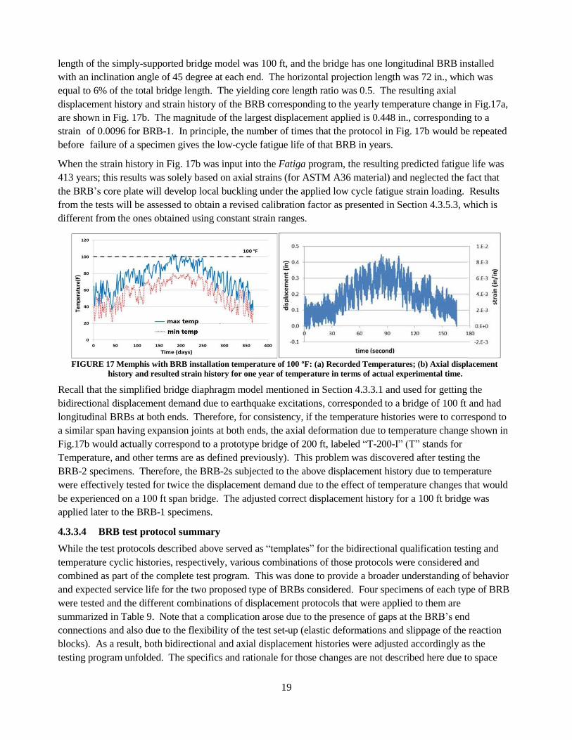
19

length of the simply-supported bridge model was 100 ft, and the bridge has one longitudinal BRB installed

with an inclination angle of 45 degree at each end. The horizontal projection length was 72 in., which was

equal to 6% of the total bridge length. The yielding core length ratio was 0.5. The resulting axial

displacement history and strain history of the BRB corresponding to the yearly temperature change in Fig.17a,

are shown in Fig. 17b. The magnitude of the largest displacement applied is 0.448 in., corresponding to a

strain of 0.0096 for BRB-1. In principle, the number of times that the protocol in Fig. 17b would be repeated

before failure of a specimen gives the low-cycle fatigue life of that BRB in years.

When the strain history in Fig. 17b was input into the Fatiga program, the resulting predicted fatigue life was

413 years; this results was solely based on axial strains (for ASTM A36 material) and neglected the fact that

the BRB’s core plate will develop local buckling under the applied low cycle fatigue strain loading. Results

from the tests will be assessed to obtain a revised calibration factor as presented in Section 4.3.5.3, which is

different from the ones obtained using constant strain ranges.

FIGURE 17 Memphis with BRB installation temperature of 100 ºF: (a) Recorded Temperatures; (b) Axial displacement

history and resulted strain history for one year of temperature in terms of actual experimental time.

Recall that the simplified bridge diaphragm model mentioned in Section 4.3.3.1 and used for getting the

bidirectional displacement demand due to earthquake excitations, corresponded to a bridge of 100 ft and had

longitudinal BRBs at both ends. Therefore, for consistency, if the temperature histories were to correspond to

a similar span having expansion joints at both ends, the axial deformation due to temperature change shown in

Fig.17b would actually correspond to a prototype bridge of 200 ft, labeled “T-200-I” (T” stands for

Temperature, and other terms are as defined previously). This problem was discovered after testing the

BRB-2 specimens. Therefore, the BRB-2s subjected to the above displacement history due to temperature

were effectively tested for twice the displacement demand due to the effect of temperature changes that would

be experienced on a 100 ft span bridge. The adjusted correct displacement history for a 100 ft bridge was

applied later to the BRB-1 specimens.

4.3.3.4 BRB test protocol summary

While the test protocols described above served as “templates” for the bidirectional qualification testing and

temperature cyclic histories, respectively, various combinations of those protocols were considered and

combined as part of the complete test program. This was done to provide a broader understanding of behavior

and expected service life for the two proposed type of BRBs considered. Four specimens of each type of BRB

were tested and the different combinations of displacement protocols that were applied to them are

summarized in Table 9. Note that a complication arose due to the presence of gaps at the BRB’s end

connections and also due to the flexibility of the test set-up (elastic deformations and slippage of the reaction

blocks). As a result, both bidirectional and axial displacement histories were adjusted accordingly as the

testing program unfolded. The specifics and rationale for those changes are not described here due to space

21

constraints, but details are presented in Wei and Bruneau (2016). Here, only test protocols and results

for BRB-2-4 and BRB-1-3 presented in this report, as illustrative examples of BRB performance.

Table 9 Summary of BRB test protocols

Specimen Test protocol TEST A TEST B TEST C TEST D TEST E

BRB-2-1* BD-E-I (to1.5 DbmL) BD-E-I BD-E-II BRB-2-2** T-200-I (85 yrs) T-200-I×1.5 (10 yrs) T-200- I×1.75(9 yrs)

BRB-2-3*** BD-E-III T-200-II (5 yrs) Axial Trial T-200-II (10 yrs) BD-E-III (cycle of 2DbmL) BRB-2-4 T-200-II (15 years) BD-E-III BRB-1-1+

BD-A-I T-100-I (75 yrs) T-100×1.37 (10 yrs) T-100×2.05 (3 yrs) BRB-1-2++

BD-A-I T-100-II T-5 (33 years) BRB-1-3+++

BD-A-II BD-A-2% BD-A-4% BD-A-6% (7 times) BRB-1-4*+

BD-N T-5 (35 years) BD-N BD-N-G (5 times) *The qualification test with BD-E-I stopped after finishing the cycle corresponding to 1.5 times the design displacement to secure the

fixture of the reaction block on the strong floor to prevent large slippage; BD-E-II has a transverse displacement demand 2.5DbmT and longitudinal displacement demand 2DbmL.

**T-200-I×j (k years) indicates that protocol T-200-I was magnified by “j” times and applied to the BRB for “k” years in order to fail

the BRB faster after finishing the required years of temperature history.

***BD-E-III was increased from BD-E-I in the longitudinal direction to account for the flexibility of the test set-up and for the pin

slippage at the BRB’s end; T-200-II was also increased from T-200-I to consider this adjustment. Axial Trial test was to ensure the

slippage of the reaction block on the shake table was reduced to acceptable values. +T-100-I is the temperature-induced axial displacement history corresponding to a 100-ft bridge with increased amplitude to account for the flexibility of the test set-up plus the bolt slippage at the BRB’s end. ++T-100-II and T-5 is scaled up from T-100-I, and also adjusted with the increased sampling rate and reduced test speed to capture the BRB’s hysteretic curve; T-5 puts the BRB under inelastic deformations of 5 times yield displacement in one year. +++BD-A-II is the average bidirectional qualification test history without longitudinal displacement adjustment; BD-A-m% means the bidirectional protocol with transverse displacement equal to “m” percent of the total BRB length applied simultaneously with a

longitudinal demand of 1.5DbmL in BD-A-II.

*+BD-N-G and BD-N stands for the actual bidirectional displacement trace of the BRB’s response to an actual ground excitation

obtained from the bridge model with and without the gap at the end bolt holes.

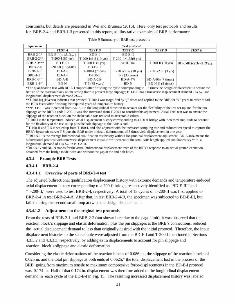
4.3.4 Example BRB Tests

4.3.4.1 BRB-2-4

4.3.4.1.1 Overview of parts of BRB-2-4 test

The adjusted bidirectional qualification displacement history with extreme demands and temperature-induced

axial displacement history corresponding to a 200-ft bridge, respectively identified as “BD-E-III” and

“T-200-II,” were used to test BRB-2-4, respectively. A total of 15 cycles of T-200-II was first applied to

BRB-2-4 in test BRB-2-4-A. After that, in test BRB-2-4-B, the specimen was subjected to BD-E-III, but

failed during the second small loop at twice the design displacement.

4.3.4.1.2 Adjustments to the original test protocols

From the tests of BRB-2-1 and BRB-2-2 (not shown here due to the page limit), it was observed that the

reaction block’s slippage and elastic deformation, plus the pin slippages at the BRB’s connections, reduced

the actual displacement demand to less than originally desired with the initial protocol. Therefore, the input

displacement histories to the shake table were adjusted from the BD-E-I and T-200-I mentioned in Sections

4.3.3.2 and 4.3.3.3, respectively, by adding extra displacements to account for pin slippage and

reaction block’s slippage and elastic deformation.

Considering the elastic deformations of the reaction blocks of 0.086 in., the slippage of the reaction blocks of

0.025 in. and the total pin slippage at both ends of 0.0625,” the total displacement lost in the process of the

BRB going from maximum tensile to maximum compressive force/displacements in the BD-E-I protocol

was 0.174 in. Half of that 0.174 in. displacement was therefore added to the longitudinal displacement

demand in each cycle of the BD-E-I in Fig. 15. The resulting increased displacement history was labeled

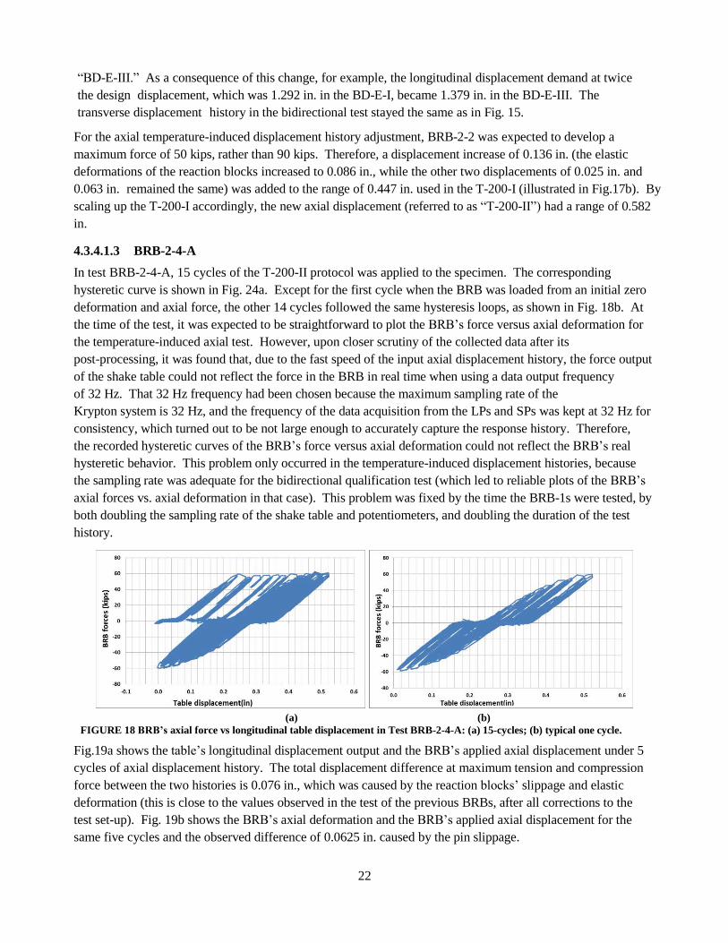
22

“BD-E-III.” As a consequence of this change, for example, the longitudinal displacement demand at twice

the design displacement, which was 1.292 in. in the BD-E-I, became 1.379 in. in the BD-E-III. The

transverse displacement history in the bidirectional test stayed the same as in Fig. 15.

For the axial temperature-induced displacement history adjustment, BRB-2-2 was expected to develop a

maximum force of 50 kips, rather than 90 kips. Therefore, a displacement increase of 0.136 in. (the elastic

deformations of the reaction blocks increased to 0.086 in., while the other two displacements of 0.025 in. and

0.063 in. remained the same) was added to the range of 0.447 in. used in the T-200-I (illustrated in Fig.17b). By

scaling up the T-200-I accordingly, the new axial displacement (referred to as “T-200-II”) had a range of 0.582

in.

4.3.4.1.3 BRB-2-4-A

In test BRB-2-4-A, 15 cycles of the T-200-II protocol was applied to the specimen. The corresponding

hysteretic curve is shown in Fig. 24a. Except for the first cycle when the BRB was loaded from an initial zero

deformation and axial force, the other 14 cycles followed the same hysteresis loops, as shown in Fig. 18b. At

the time of the test, it was expected to be straightforward to plot the BRB’s force versus axial deformation for

the temperature-induced axial test. However, upon closer scrutiny of the collected data after its

post-processing, it was found that, due to the fast speed of the input axial displacement history, the force output

of the shake table could not reflect the force in the BRB in real time when using a data output frequency

of 32 Hz. That 32 Hz frequency had been chosen because the maximum sampling rate of the

Krypton system is 32 Hz, and the frequency of the data acquisition from the LPs and SPs was kept at 32 Hz for

consistency, which turned out to be not large enough to accurately capture the response history. Therefore,

the recorded hysteretic curves of the BRB’s force versus axial deformation could not reflect the BRB’s real

hysteretic behavior. This problem only occurred in the temperature-induced displacement histories, because

the sampling rate was adequate for the bidirectional qualification test (which led to reliable plots of the BRB’s

axial forces vs. axial deformation in that case). This problem was fixed by the time the BRB-1s were tested, by

both doubling the sampling rate of the shake table and potentiometers, and doubling the duration of the test

history.

(a) (b)

FIGURE 18 BRB’s axial force vs longitudinal table displacement in Test BRB-2-4-A: (a) 15-cycles; (b) typical one cycle.

Fig.19a shows the table’s longitudinal displacement output and the BRB’s applied axial displacement under 5

cycles of axial displacement history. The total displacement difference at maximum tension and compression

force between the two histories is 0.076 in., which was caused by the reaction blocks’ slippage and elastic

deformation (this is close to the values observed in the test of the previous BRBs, after all corrections to the

test set-up). Fig. 19b shows the BRB’s axial deformation and the BRB’s applied axial displacement for the

same five cycles and the observed difference of 0.0625 in. caused by the pin slippage.

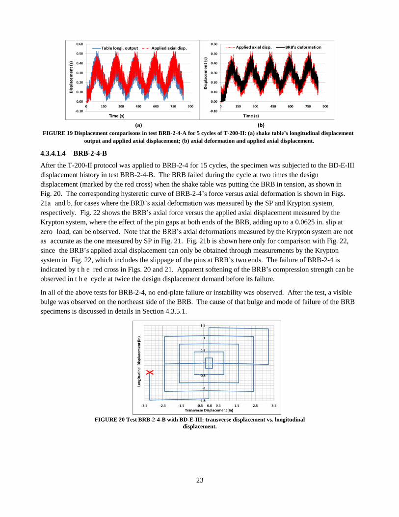
23

(a) (b)

FIGURE 19 Displacement comparisons in test BRB-2-4-A for 5 cycles of T-200-II: (a) shake table’s longitudinal displacement

output and applied axial displacement; (b) axial deformation and applied axial displacement.

4.3.4.1.4 BRB-2-4-B

After the T-200-II protocol was applied to BRB-2-4 for 15 cycles, the specimen was subjected to the BD-E-III

displacement history in test BRB-2-4-B. The BRB failed during the cycle at two times the design

displacement (marked by the red cross) when the shake table was putting the BRB in tension, as shown in

Fig. 20. The corresponding hysteretic curve of BRB-2-4’s force versus axial deformation is shown in Figs.

21a and b, for cases where the BRB’s axial deformation was measured by the SP and Krypton system,

respectively. Fig. 22 shows the BRB’s axial force versus the applied axial displacement measured by the

Krypton system, where the effect of the pin gaps at both ends of the BRB, adding up to a 0.0625 in. slip at

zero load, can be observed. Note that the BRB’s axial deformations measured by the Krypton system are not

as accurate as the one measured by SP in Fig. 21. Fig. 21b is shown here only for comparison with Fig. 22,

since the BRB’s applied axial displacement can only be obtained through measurements by the Krypton

system in Fig. 22, which includes the slippage of the pins at BRB’s two ends. The failure of BRB-2-4 is

indicated by t h e red cross in Figs. 20 and 21. Apparent softening of the BRB’s compression strength can be

observed in t h e cycle at twice the design displacement demand before its failure.

In all of the above tests for BRB-2-4, no end-plate failure or instability was observed. After the test, a visible

bulge was observed on the northeast side of the BRB. The cause of that bulge and mode of failure of the BRB

specimens is discussed in details in Section 4.3.5.1.

FIGURE 20 Test BRB-2-4-B with BD-E-III: transverse displacement vs. longitudinal

displacement.

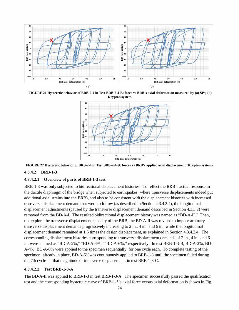
24

(a) (b)

FIGURE 21 Hysteretic behavior of BRB-2-4 in Test BRB-2-4-B: force vs BRB’s axial deformation measured by (a) SPs; (b)

Krypton system.

FIGURE 22 Hysteretic behavior of BRB-2-4 in Test BRB-2-4-B: forces vs BRB’s applied axial displacement (Krypton system).

4.3.4.2 BRB-1-3

4.3.4.2.1 Overview of parts of BRB-1-3 test

BRB-1-3 was only subjected to bidirectional displacement histories. To reflect the BRB’s actual response in

the ductile diaphragm of the bridge when subjected to earthquakes (where transverse displacements indeed put

additional axial strains into the BRB), and also to be consistent with the displacement histories with increased

transverse displacement demand that were to follow (as described in Section 4.3.4.2.4), the longitudinal

displacement adjustments (caused by the transverse displacement demand described in Section 4.3.3.2) were

removed from the BD-A-I. The resulted bidirectional displacement history was named as “BD-A-II.” Then,

t o explore the transverse displacement capacity of the BRB, the BD-A-II was revised to impose arbitrary

transverse displacement demands progressively increasing to 2 in., 4 in., and 6 in., while the longitudinal

displacement demand remained at 1.5 times the design displacement, as explained in Section 4.3.4.2.4. The

corresponding displacement histories corresponding to transverse displacement demands of 2 in., 4 in., and 6

in. were named as “BD-A-2%,” “BD-A-4%,” “BD-A-6%,” respectively. In test BRB-1-3-B, BD-A-2%, BD-

A-4%, BD-A-6% were applied to the specimen sequentially, for one cycle each. To complete testing of the

specimen already in place, BD-A-6%was continuously applied to BRB-1-3 until the specimen failed during

the 7th cycle at that magnitude of transverse displacement, in test BRB-1-3-C.

4.3.4.2.2 Test BRB-1-3-A

The BD-A-II was applied to BRB-1-3 in test BRB-1-3-A. The specimen successfully passed the qualification

test and the corresponding hysteretic curve of BRB-1-3’s axial force versus axial deformation is shown in Fig.

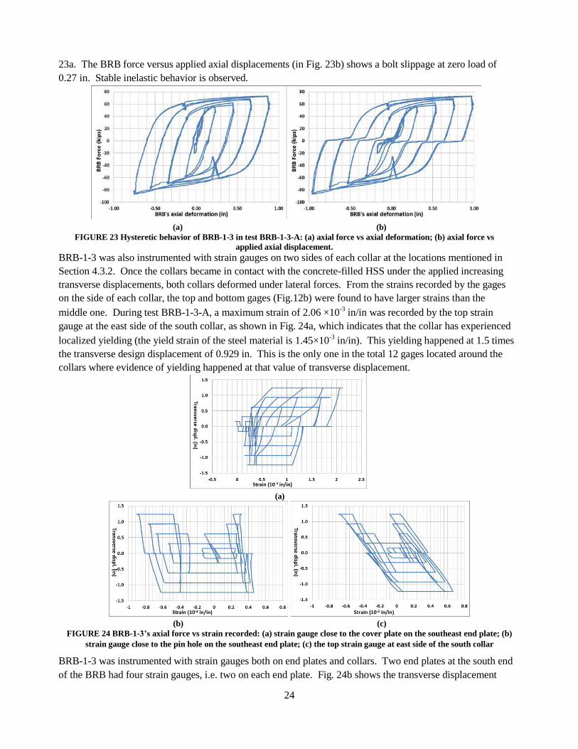
23a. The BRB force versus applied axial displacements (in Fig. 23b) shows a bolt slippage at zero load of

0.27 in. Stable inelastic behavior is observed.

(a) (b)

FIGURE 23 Hysteretic behavior of BRB-1-3 in test BRB-1-3-A: (a) axial force vs axial deformation; (b) axial force vs

applied axial displacement.

BRB-1-3 was also instrumented with strain gauges on two sides of each collar at the locations mentioned in

Section 4.3.2. Once the collars became in contact with the concrete-filled HSS under the applied increasing

transverse displacements, both collars deformed under lateral forces. From the strains recorded by the gages

on the side of each collar, the top and bottom gages (Fig.12b) were found to have larger strains than the

middle one. During test BRB-1-3-A, a maximum strain of 2.06 ×10-3

in/in was recorded by the top strain

gauge at the east side of the south collar, as shown in Fig. 24a, which indicates that the collar has experienced

localized yielding (the yield strain of the steel material is 1.45×10-3

in/in). This yielding happened at 1.5 times

the transverse design displacement of 0.929 in. This is the only one in the total 12 gages located around the

collars where evidence of yielding happened at that value of transverse displacement.

(a)

(b) (c)

FIGURE 24 BRB-1-3’s axial force vs strain recorded: (a) strain gauge close to the cover plate on the southeast end plate; (b)

strain gauge close to the pin hole on the southeast end plate; (c) the top strain gauge at east side of the south collar

BRB-1-3 was instrumented with strain gauges both on end plates and collars. Two end plates at the south end

of the BRB had four strain gauges, i.e. two on each end plate. Fig. 24b shows the transverse displacement

24

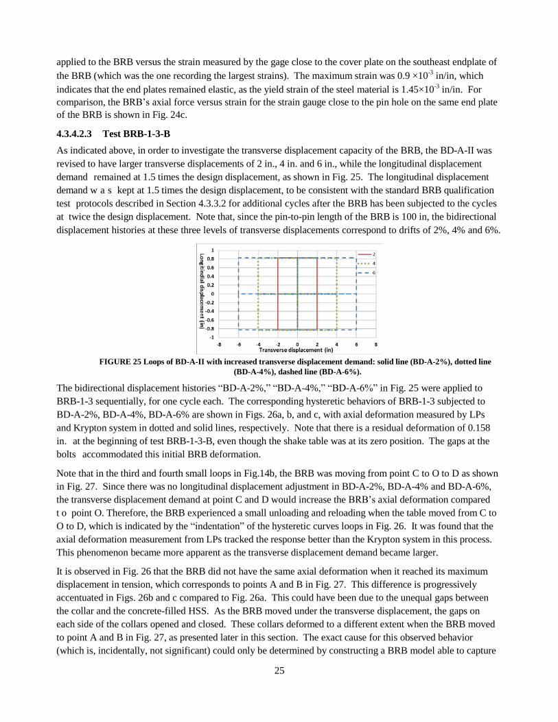
25

applied to the BRB versus the strain measured by the gage close to the cover plate on the southeast endplate of

the BRB (which was the one recording the largest strains). The maximum strain was 0.9 ×10-3

in/in, which

indicates that the end plates remained elastic, as the yield strain of the steel material is 1.45×10-3

in/in. For

comparison, the BRB’s axial force versus strain for the strain gauge close to the pin hole on the same end plate

of the BRB is shown in Fig. 24c.

4.3.4.2.3 Test BRB-1-3-B

As indicated above, in order to investigate the transverse displacement capacity of the BRB, the BD-A-II was

revised to have larger transverse displacements of 2 in., 4 in. and 6 in., while the longitudinal displacement

demand remained at 1.5 times the design displacement, as shown in Fig. 25. The longitudinal displacement

demand w a s kept at 1.5 times the design displacement, to be consistent with the standard BRB qualification

test protocols described in Section 4.3.3.2 for additional cycles after the BRB has been subjected to the cycles

at twice the design displacement. Note that, since the pin-to-pin length of the BRB is 100 in, the bidirectional

displacement histories at these three levels of transverse displacements correspond to drifts of 2%, 4% and 6%.

FIGURE 25 Loops of BD-A-II with increased transverse displacement demand: solid line (BD-A-2%), dotted line

(BD-A-4%), dashed line (BD-A-6%).

The bidirectional displacement histories “BD-A-2%,” “BD-A-4%,” “BD-A-6%” in Fig. 25 were applied to

BRB-1-3 sequentially, for one cycle each. The corresponding hysteretic behaviors of BRB-1-3 subjected to

BD-A-2%, BD-A-4%, BD-A-6% are shown in Figs. 26a, b, and c, with axial deformation measured by LPs

and Krypton system in dotted and solid lines, respectively. Note that there is a residual deformation of 0.158

in. at the beginning of test BRB-1-3-B, even though the shake table was at its zero position. The gaps at the

bolts accommodated this initial BRB deformation.

Note that in the third and fourth small loops in Fig.14b, the BRB was moving from point C to O to D as shown

in Fig. 27. Since there was no longitudinal displacement adjustment in BD-A-2%, BD-A-4% and BD-A-6%,

the transverse displacement demand at point C and D would increase the BRB’s axial deformation compared

t o point O. Therefore, the BRB experienced a small unloading and reloading when the table moved from C to

O to D, which is indicated by the “indentation” of the hysteretic curves loops in Fig. 26. It was found that the

axial deformation measurement from LPs tracked the response better than the Krypton system in this process.

This phenomenon became more apparent as the transverse displacement demand became larger.

It is observed in Fig. 26 that the BRB did not have the same axial deformation when it reached its maximum

displacement in tension, which corresponds to points A and B in Fig. 27. This difference is progressively

accentuated in Figs. 26b and c compared to Fig. 26a. This could have been due to the unequal gaps between

the collar and the concrete-filled HSS. As the BRB moved under the transverse displacement, the gaps on

each side of the collars opened and closed. These collars deformed to a different extent when the BRB moved

to point A and B in Fig. 27, as presented later in this section. The exact cause for this observed behavior

(which is, incidentally, not significant) could only be determined by constructing a BRB model able to capture

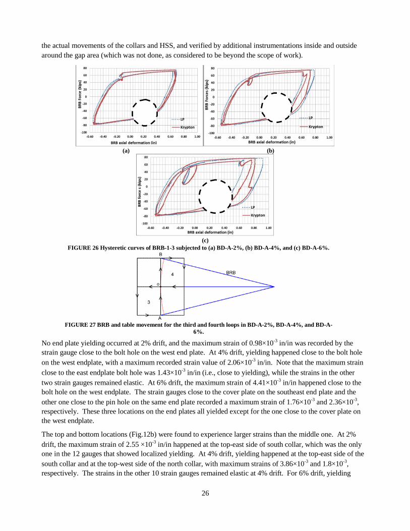
26

the actual movements of the collars and HSS, and verified by additional instrumentations inside and outside

around the gap area (which was not done, as considered to be beyond the scope of work).

(a) (b)

(c)

FIGURE 26 Hysteretic curves of BRB-1-3 subjected to (a) BD-A-2%, (b) BD-A-4%, and (c) BD-A-6%.

FIGURE 27 BRB and table movement for the third and fourth loops in BD-A-2%, BD-A-4%, and BD-A-

6%.

No end plate yielding occurred at 2% drift, and the maximum strain of 0.98×10-3

in/in was recorded by the

strain gauge close to the bolt hole on the west end plate. At 4% drift, yielding happened close to the bolt hole

on the west endplate, with a maximum recorded strain value of 2.06×10-3

in/in. Note that the maximum strain

close to the east endplate bolt hole was 1.43×10-3

in/in (i.e., close to yielding), while the strains in the other

two strain gauges remained elastic. At 6% drift, the maximum strain of 4.41×10-3

in/in happened close to the

bolt hole on the west endplate. The strain gauges close to the cover plate on the southeast end plate and the

other one close to the pin hole on the same end plate recorded a maximum strain of 1.76×10-3

and 2.36×10-3

,

respectively. These three locations on the end plates all yielded except for the one close to the cover plate on

the west endplate.

The top and bottom locations (Fig.12b) were found to experience larger strains than the middle one. At 2%

drift, the maximum strain of 2.55 ×10-3

in/in happened at the top-east side of south collar, which was the only

one in the 12 gauges that showed localized yielding. At 4% drift, yielding happened at the top-east side of the

south collar and at the top-west side of the north collar, with maximum strains of 3.86×10-3

and 1.8×10-3

,

respectively. The strains in the other 10 strain gauges remained elastic at 4% drift. For 6% drift, yielding

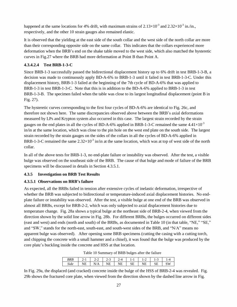
27

happened at the same locations for 4% drift, with maximum strains of 2.13×10-3

and 2.32×10-3

in./in.,

respectively, and the other 10 strain gauges also remained elastic.

It is observed that the yielding at the east side of the south collar and the west side of the north collar are more

than their corresponding opposite side on the same collar. This indicates that the collars experienced more

deformation when the BRB’s end on the shake table moved to the west side, which also matched the hysteretic

curves in Fig.27 where the BRB had more deformation at Point B than Point A.

4.3.4.2.4 Test BRB-1-3-C

Since BRB-1-3 successfully passed the bidirectional displacement history up to 6% drift in test BRB-1-3-B, a

decision was made to continuously apply BD-A-6% to BRB-1-3 until it failed in test BRB-1-3-C. Under this

displacement history, BRB-1-3 failed at the beginning of the 7th cycle of BD-A-6% that was applied to

BRB-1-3 in test BRB-1-3-C. Note that this is in addition to the BD-A-6% applied to BRB-1-3 in test

BRB-1-3-B. The specimen failed when the table was close to its largest longitudinal displacement (point B in

Fig. 27).

The hysteretic curves corresponding to the first four cycles of BD-A-6% are identical to Fig. 26c, and

therefore not shown here. The same discrepancies observed above between the BRB’s axial deformations

measured by LPs and Krypton system also occurred in this case. The largest strain recorded by the strain

gauges on the end plates in all the cycles of BD-A-6% applied in BRB-1-3-C remained the same 4.41×10-3

in/in at the same location, which was close to the pin hole on the west end plate on the south side. The largest

strain recorded by the strain gauges on the sides of the collars in all the cycles of BD-A-6% applied in

BRB-1-3-C remained the same 2.32×10-3

in/in at the same location, which was at top of west side of the north

collar.

In all of the above tests for BRB-1-3, no end-plate failure or instability was observed. After the test, a visible

bulge was observed on the southeast side of the BRB. The cause of that bulge and mode of failure of the BRB

specimens will be discussed in details in Section 4.3.5.1.

4.3.5 Investigation on BRB Test Results

4.3.5.1 Observations on BRB’s failure

As expected, all the BRBs failed in tension after extensive cycles of inelastic deformation, irrespective of

whether the BRB was subjected to bidirectional or temperature-induced axial displacement histories. No end-

plate failure or instability was observed. After the test, a visible bulge at one end of the BRB was observed in

almost all BRBs, except for BRB-2-2, which was only subjected to axial displacement histories due to

temperature change. Fig. 28a shows a typical bulge at the northeast side of BRB-2-4, when viewed from the

direction shown by the solid line arrow in Fig. 28b. For different BRBs, the bulges occurred on different sides

(east and west) and ends (north and south) of the BRBs, as documented in Table 10 (in that table, “NE,” “SE,”

and “SW,” stands for the north-east, south-east, and south-west sides of the BRB, and “N/A” means no

apparent bulge was observed). After opening some BRB specimens (cutting the casing with a cutting torch,

and chipping the concrete with a small hammer and a chisel), it was found that the bulge was produced by the

core plate’s buckling inside the concrete and HSS at that location.

Table 10 Summary of BRB bulges after the failure

BRB 2-1 2-2 2-3 2-4 1-1 1-2 1-3 1-4

Side NE N/A NE NE SE NE SE SW

In Fig. 29a, the displaced (and cracked) concrete inside the bulge of the HSS of BRB-2-4 was revealed. Fig.

29b shows the fractured core plate, when viewed from the direction shown by the dashed line arrow in Fig.

28

28b. Visibly significant out-of-plane displacement of the core plate had occurred and was the cause of the

observed bulges. Fig. 30 shows part of the core plate in the vicinity of where it fractured. That fracture

occurred at the tip of a severe and isolated local buckle. The circled part of the core plate shown in Fig. 30 is

similarly circled in Fig. 31 to show that failure typically occurred in the part of the core plate close to the

transition zone (typically at one of the two locations shown in Fig. 31). Note that when fracture occurred at

one of the two circled location in Fig. 31, at the opposite location close to the other transition part of the core

plate, significant out-of-plane deformation of the core plate also happened, but it had smaller amplitude than

where failure occurred. Specific manufacturing details of the tested BRB (that cannot be revealed) were found

to explain why the BRB core plate could more easily buckle at those two locations, and recommendations

were made to the BRB manufacturer that could enhance the low fatigue life of the BRB (although one must

keep in mind that the BRBs already all exhibited considerable cumulative ductilities, as shown in Section

4.3.5.2 below). Note that except for these two circled part in Fig. 31, the rest of the core plate remained

mostly straight (as verified using a straight edge).

(a) (b)

FIGURE 28 Bulge on the NE side of the HSS of BRB-2-4.

(a) (b)

FIGURE 29 BRB-2-4’s failure observation: (a) Concrete fractured around the broken core plate of BRB-2-4; (b) Broken

section of BRB-2-4’s core plate

FIGURE 30 Part of the core plate of BRB-2-4 with the fracture.

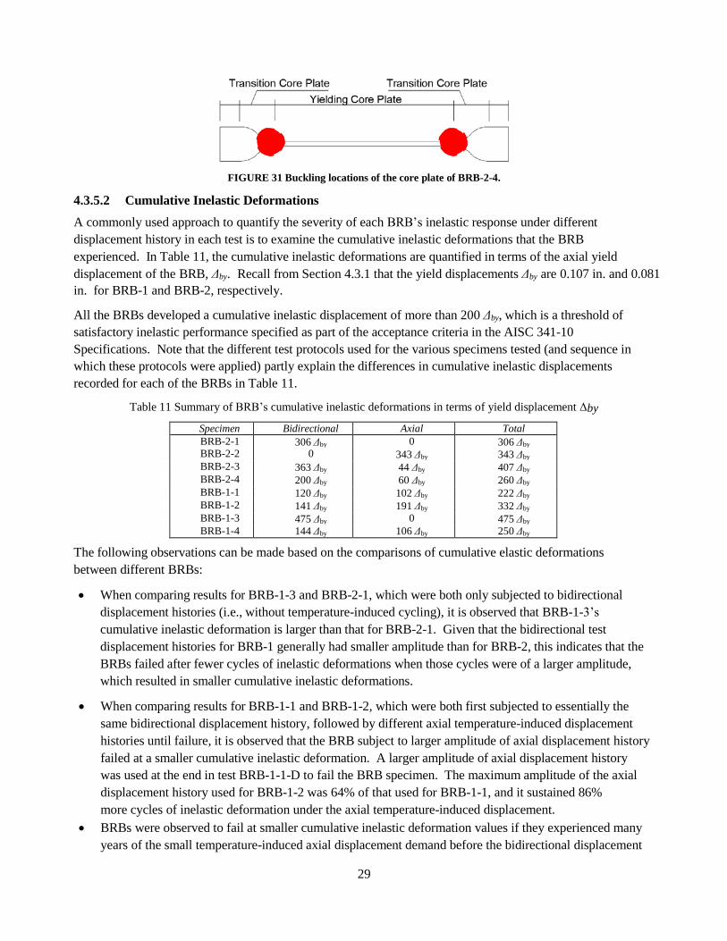
29

FIGURE 31 Buckling locations of the core plate of BRB-2-4.

4.3.5.2 Cumulative Inelastic Deformations

A commonly used approach to quantify the severity of each BRB’s inelastic response under different

displacement history in each test is to examine the cumulative inelastic deformations that the BRB

experienced. In Table 11, the cumulative inelastic deformations are quantified in terms of the axial yield

displacement of the BRB, Δby. Recall from Section 4.3.1 that the yield displacements Δby are 0.107 in. and 0.081

in. for BRB-1 and BRB-2, respectively.

All the BRBs developed a cumulative inelastic displacement of more than 200 Δby, which is a threshold of

satisfactory inelastic performance specified as part of the acceptance criteria in the AISC 341-10

Specifications. Note that the different test protocols used for the various specimens tested (and sequence in

which these protocols were applied) partly explain the differences in cumulative inelastic displacements

recorded for each of the BRBs in Table 11.

Table 11 Summary of BRB’s cumulative inelastic deformations in terms of yield displacement Δby

Specimen Bidirectional Axial Total

BRB-2-1 306 Δby 0 306 Δby

BRB-2-2 0 343 Δby 343 Δby

BRB-2-3 363 Δby 44 Δby 407 Δby

BRB-2-4 200 Δby 60 Δby 260 Δby

BRB-1-1 120 Δby 102 Δby 222 Δby

BRB-1-2 141 Δby 191 Δby 332 Δby

BRB-1-3 475 Δby 0 475 Δby

BRB-1-4 144 Δby 106 Δby 250 Δby

The following observations can be made based on the comparisons of cumulative elastic deformations

between different BRBs:

When comparing results for BRB-1-3 and BRB-2-1, which were both only subjected to bidirectional

displacement histories (i.e., without temperature-induced cycling), it is observed that BRB-1-3’s

cumulative inelastic deformation is larger than that for BRB-2-1. Given that the bidirectional test

displacement histories for BRB-1 generally had smaller amplitude than for BRB-2, this indicates that the

BRBs failed after fewer cycles of inelastic deformations when those cycles were of a larger amplitude,

which resulted in smaller cumulative inelastic deformations.

When comparing results for BRB-1-1 and BRB-1-2, which were both first subjected to essentially the

same bidirectional displacement history, followed by different axial temperature-induced displacement

histories until failure, it is observed that the BRB subject to larger amplitude of axial displacement history

failed at a smaller cumulative inelastic deformation. A larger amplitude of axial displacement history

was used at the end in test BRB-1-1-D to fail the BRB specimen. The maximum amplitude of the axial

displacement history used for BRB-1-2 was 64% of that used for BRB-1-1, and it sustained 86%

more cycles of inelastic deformation under the axial temperature-induced displacement.

BRBs were observed to fail at smaller cumulative inelastic deformation values if they experienced many

years of the small temperature-induced axial displacement demand before the bidirectional displacement

30

demands from the earthquake was applied to it. This can be seen by comparing results for BRB-2-3 and

BRB-2-4. Recall that a temperature-induced displacement history (corresponding to 60Δby) was first

applied to BRB-2-4 before the extreme bidirectional displacement history (corresponding to 200Δby) was

applied to it. In the test of BRB-2-3, the BRB was first subjected to a bidirectional displacement history

(corresponding to 245 Δby), followed then by the same temperature-induced axial displacement history

but with a different number of cycles (corresponding to 44 Δby), and ending with more cycles of

bidirectional displacement history (corresponding to 118 Δby). BRB-2-3 reached 156% more cumulative

inelastic deformation than BRB-2-4. This result suggests that the sequence in which the different

displacement histories are applied could matter.

Note that all the BRBs reached cumulative inelastic deformations of 250Δby, except for BRB-1-1. In BRB-1-1,

which reached only 222Δby, the temperature-induced axial displacement history was scaled up to a large

magnitude at the end of the test, with the intention to fail BRB-1-1 quicker, and it is possible that this has

reduced the fatigue life. However, more tests would be needed to provide a statistical basis to validate the

above observations. Although the BRBs were identical in their design, some subtle (but not easily visible)

differences in how they were fabricated could also be responsible for the observed differences.

From a design perspective, the above information could be used to assess how many years a BRB could remain

in service while retaining its ability to provide adequate seismic response. For example, for a bridge

with the length, L, in Memphis installed with a longitudinal BRB having a steel core length of 6% with no

inclination (i.e., installed horizontally) at each end in the EDS, the number of years depends on BRB’s design

displacement demand from the earthquake (which is chosen to correspond to a ductility, μB , of 6 in this

example). Note that the cumulative inelastic deformation in the AISC axial qualification test protocol equals

to 8×(5μB -4), which gives 208 Δby for a ductility of 6. If the maximum cumulative inelastic deformation of the

BRB of 250Δby is used here, this leaves 42Δby available for the cumulative inelastic deformations of the BRB

subjected to the temperature displacement history. For a BRB’s steel core plate having yield strength and

Young’s modulus of 46 ksi and 29000 ksi, the yield displacement of the BRB based on deformation only in

the core length, Δby, equals to 9.52×10-5

L (i.e.,= 46/29000×0.06L). For the case at hand (Memphis), the

maximum and minimum yearly temperatures are 102ºF and 20ºF, and the temperature range, ΔT, is 82ºF (from

Fig. 17a). Assuming that the bridge’s concrete slab governs its thermal expansion, and using the coefficient of

thermal expansion of concrete, αc, of 0.000006 in/in/°F to calculate the one-year temperature displacement

history applied to the BRB as 0.5αcLΔT (the tributary length of the bridge for each longitudinal

BRB is 0.5L). The corresponding inelastic deformation of the BRB is αcLΔT-4Δby, equal to 1.17Δby. Therefore,

the number of years that the BRB can be installed in the EDS of this bridge is approximately 35 years. Note

that the number of years in service would be greater if gaps in the end connections of the BRB absorbed some

of these thermal displacements.

4.3.5.3 Low-cycle fatigue damage

Recall, from Section 4.2.2, that the fatigue life of the BRB can be predicted using the Fatiga program, using

input strain history calculated from displacements applied to the BRB due to the temperature changes of the

bridge. In this section, the fatigue life and damage are studied based on the experimental results. The

deformations output from the LPs were used to obtain the strain history of the core plate during each test.

Then, they were input in Fatiga individually to get the fatigue damage, as shown in Table 12. Since the BRB

failed after applying these displacement histories, the total damage factor is also the calibration factor, which

relates the base-metal low-cycle failure to that of a BRB which will ultimately fracture due to repeated local

buckling of the core plate as mentioned in Section 4.2.2. The calibration factors obtained range from 0.0122

to 0.0486, with an average of 0.0363. Note that for the BRB tested in the literature using cycles of constant

31

strain amplitude (described in Section 4.2.2), calibration factors ranging from 0.05 to 0.53 were reported. For

strain ranges comparable to those reached during the tests in Section 4.2.2, these factors from past experiments

ranged from 0.05 to 0.11. The BRBs calibration factors obtained as part of the research conducted here are

smaller than those reported in the literature. However, one must keep in mind that fatigue damage is

dependent on the magnitude of the strain ranges and the cycles sequence in the strain history, but also on the

type of BRB tested because different BRB detailing can lead to the development of different types of local

buckling of the steel core.

Here, the reported calibration factors can be used to allow predicting the fatigue life of the BRB from a

low-cycle fatigue perspective. However, more experimental works would be needed to provide a statistical

basis to generate generic predicting calibration factors for BRBs, based on the type of BRB specimen, as well

as the magnitude and sequence of the applied strain history.

Table 12 Summary of BRB’s fatigue damage

Specimen Bidirectional Axial Total Damage

BRB-2-1 0.0122 0 0.0122

BRB-2-2 0 0.0486 0.0486

BRB-2-3 0.0225 0.0100 0.0325

BRB-2-4 0.0085 0.0050 0.0135

BRB-1-1 0.0097 0.0275 0.0372

BRB-1-2 0.0103 0.0248 0.0351

BRB-1-3 0.0416 0 0.0416

BRB-1-4 0.0104 0.0351 0.0455

4.4 Design Procedures

On the basis of the above findings, the following procedure is proposed to design bidirectional bridge end

diaphragms for a given bridge at a known location:

a. Assume an initial value for the fundamental period of the EDS, Teff. In this procedure, the EDS period is

the same for the longitudinal and transverse direction. For a skew bridge, that would be the value for an

equivalent non-skew EDS.

b. For the specified design acceleration response spectrum at the bridge location, which gives the elastic

force demand of the bridge, mSa, at its fundamental period, Teff , choose a desired displacement ductility of

the non-skew bridge EDS, μ, the maximum of which can be taken as 6 per Equation 4.3.3 in AASHTO

(2011); calculate the corresponding force reduction factor, R according to Equations 1 and 2 in Section

4.2.1.2.1.

c. The yield strength of the non-skew EDS, Vy, is mSa/R, and the stiffness, Keff , is 4π2m/Teff

2, and the yield

displacement of the EDS, δy ,is Vy/Keff . The resulting inelastic displacement demand of the non-skew EDS

is the elastic spectral displacement, δyμ, times the inelastic displacement magnification factor, Rd1,

specified in Section 4.2.1.2.2.

d. Determine the displacement limits of the EDS: (1) the limit in the longitudinal directions, δLm, is the gap

between the bridge deck and abutment or the maximum seat width available; (2) the limit in the transverse

directions, δTm , is the girder lateral yield displacement (for diaphragms with energy dissipator connected

between girders), calculated based on the girder properties for a given steel bridge. Changes to the bridge

design can be made to ensure that these two values are greater than the displacement demands calculated

in Step c. Alternatively, iterations over steps a to c may be needed until the resulting displacement

demands δu in both directions are smaller than the limit.

e. For the bridge with skewness, the skew EDS is designed to have the same yield strength and displacement

as its equivalent non-skew EDS designed following steps a to d. The displacement demand of the skew

EDS, δu , is calculated as δyμRd1Rd2, where Rd2 is a displacement magnification factor,Rd2, relating the

expected maximum displacement response of skew bridge to that of its equivalent non-skew bridge, and

specified in Section 4.2.1.2.4.

32

f. Determine the local displacement demand of the BRB based on the above displacement demand of the

EDS, δu.

g. Design the BRB in the EDS following either of the three approaches presented below in item (1), (2), and

(3), while satisfying the requirements in item (4) and (5):

1) Implicit Design: Select the minimum length of the longitudinal BRB’s steel core to be at least 6% of

the total length of the bridge (one longitudinal BRB at each end of the bridge). Based on the above

findings (i.e., BRB having maximum cumulative inelastic deformations of 250 times the yield

deformation as described in Section 4.3.5.3), this BRB can be left in service for 35 years and expected

to resist the seismic demand corresponding to a ductility of 6. This value can be modified to take into

account the inclination of the BRB to reduce the length of the BRB yielding core as a percentage of

total bridge length (see Section 4.2.2).

2) Explicit Design: Select a longitudinal BRB yielding steel core length, such that the sum of the

cumulative ductilities corresponding to temperature-induced displacement demand and cyclic testing

protocol (both calculated following the example in Section 4.3.5.2) does not exceed 250Δby. This may

require iterations varying the length of BRB steel core, the desired number of years in service, and the

expected BRB’s ductility to resist the seismic demand.

3) Qualification Testing (to be used if the above cumulative inelastic displacement limit of 250Δby is

deemed too restrictive): BRB designs can be qualified by subjecting one BRB to: (i) the BRB standard

test protocols (following AISC 341-10), followed by; (ii) the temperature-induced axial displacement

history protocols applied repetitively for the number of years of service that the BRB is expected to

provide in addition to the satisfactory seismic response; and a second identical BRB subjected to the

same protocols (i) and (ii) but applied in the reverse order (i.e., (ii) followed by (i)). This qualification

testing approach would be of benefit for BRBs of different fabrication/detailing (and possibly sizes)

than those considered in this research project.

4) Determine the BRBs’ end connections by: (i) designing the end plates of the BRB to bend laterally to

accommodate the required lateral displacement without developing instability; (ii) connecting the end

plates of the BRB to a spherical bearing (note that special protection would be required to prevent

corrosion of the spherical bearings).

5) Design the BRB connecting gusset plate to resist 1.5 times the BRB yield strength. Limitations for

the maximum gusset plate length and corresponding thickness are provided to ensure that the BRB

can sustain the displacements demands without flexural yielding of the gusset plate connection.

5 FINDINGS AND CONCLUSIONS

Analytical and experimental work conducted as part of this project has demonstrated the feasibility of

implementing bidirectional ductile diaphragm in both skew and non-skew bridges. Quasi-static tests have

demonstrated that BRBs having specially designed end connection details (such as having either long end

plates designed to provide adequate buckling resistance, or spherical bearing, designed per the procedure

presented in Section 4.3.1) are able to sustain extensive cycles of inelastic deformations without end-plate

failure or instability. Tests up to low-cycle fatigue failure on eight BRBs (presented in Section 4.3.4) have

demonstrated that the BRB specimens developed cumulative inelastic deformations of more than 250 times

the BRB’s axial yield displacement, under different sequences of bidirectional and temperature-induced axial

displacement test protocols designed to simulate demands when used in bidirectional ductile diaphragms.

Based on findings from this research program, a procedure has been formulated (Section 4.4) to design BRBs

in ductile diaphragms, and to establish when they should be replaced during the life of the bridge, using the

cumulative ductililty of 250 times the yield displacement as a performance basis. However, the design

procedure also specifies a test protocol that can be used to extend this limit, as it is foreseen that other BRBs

designs/detailing could allow reaching significantly greater cumulative ductilities.

33

6 PLANS FOR IMPLEMENTATION

To transition this technology to field applications, an NCHRP IDEA Type 2 project is recommended to test a

scale-model of a complete bridge span using a shake table to verify the dynamic response of a complete

system in which the bi-directional ductile diaphragm concept is implemented. BRBs designs from various

suppliers should be sequentially tested as part of this shake-table test series, to broaden the understanding of

how various BRB details could impact system response. The scope of this Type 2 project would also include

investigating implementation of the bidirectional diaphragm concept in various configurations of multi-span

bridges. Results from both the Type 1 and Type 2 research will then be used to formulate design guidelines of

bidirectional ductile diaphragms to resist earthquakes from any directions regardless of skewness. These could

then be formulated in a language ready for implementation by AASHTO (via T3 Seismic and T14 Steel

Design) and by Departments of Transportation.

7 REFERENCES

1) AASHTO (2012). LRFD Bridge Design Specifications, 6th ed., American Association of State Highway and

Transportation Officials, Washington, D.C.

2) AASHTO (2011). Guide Specifications for LRFD Seismic Bridge Design, 2nd ed., Washington, D.C., 248 pp.

3) AccuWeather (2012). Retrieved from http://www.accuweather.com/.

4) AISC-341 (2010). “Seismic Provisions for Structural Steel Buildings,” American Institute of Steel

Construction, Chicago, Ill.

5) Akira, W. (2000). Fatigue Properties of Practical-Scale Unbonded Braces, Nippon Steel Technical Report 82.

6) ATC49 (2001), “Recommended LRFD Guidelines for the Seismic Design of Highway Bridges,” prepared by the

Applied Technology Council.

7) Basquin, O.H. (1910). “The Exponential Law of Endurance Test,” Proc., American Society for Testing and

Materials, Vol.10, Part II, pp. 625–630.

8) Bruneau, M., C.M. Uang, and R. Sabelli (2011). Ductile Design of Steel Structures, 2nd ed., McGraw–Hill, New

York, N.Y., 921 pp.

9) Coffin, L.F. (1953). “A Study of the Effects of Cyclic Thermal Stresses on a Ductile Metal,” Trans. ASME, Vol. 76, pp.

931–950.

10) Fatiga Version 1.03 [computer software], Fatec Engineering, Bergschenhoek, the Netherlands.

11) FEMA P-695 (2009). “Quantification of Building Seismic Performance Factors,” prepared by Applied Technology

C ouncil for FEMA, Washington, D.C.

12) Kanaji H., M. Kitazawa, and N. Suzuki (2003). “Seismic Retrofit Strategy Using Damage Control Design Concept

and the Response Reduction Effect for a Long-Span Truss Bridge, 19th U.S.–Japan Bridge Engineering Workshop Panel on Wind and Seismic Effects, UJNR, Tsukuba Science City, Japan.

13) López, W.A. and R. Sabelli (2004). Steel Tips Report: Seismic Design of Buckling-Restrained Braced Frames,

Structural Steel Educational Council, California.

14) Maeda, Y., Y. Nakata, M. Iwata, and A. Wada (1998). “Fatigue Properties of Axial-Yield Type Hsteresis

Dampers,” J. Struct. Constr. Eng., Vol. 503, pp. 109–115.

15) Manson, S.S. (1952). “Behavior of Materials Under Conditions of Thermal Stress,” presented at the Symposium on

Heat Transfer, University of Michigan.

16) Miranda E. and V.V. Bertero (1994), “Evaluation of Strength Reduction Factor for Earthquake-Resistant

Design,” Earthquake Spectra, Vol. 10, No. 2, 1994.

17) OpenSees Version 2.4.6 [computer software], University of California.

18) SAP2000 Version 14 [computer software], Computers & Structures. Inc., California. 19) Sarraf, M. and M. Bruneau (1998a). "Ductile Seismic Retrofit of Steel Deck-Truss Bridges. I: Strategy and

Modeling," J. Struct. Eng., Vol. 124, No. 11, pp. 1253–1262.

20) Sarraf, M., and M. Bruneau (1998b). "Ductile Seismic Retrofit of Steel Deck-Truss Bridges. II: Design Applications,"

J. Struct. Eng., Vol. 124, No. 11, pp. 1263–1271.

21) Smith, K.N., P . Watson, and T.H. Topper (1970). “A Stress-Strain F unction for the F atigue of M etals,”

Journal of Materials, ASTM, Vol. 5, pp. 767–778.

22) Usami, T., C. Wang, and J . Funayama (2011). "Low-Cycle Fatigue Tests of a Type of Buckling Restrained

Braces," Procedia Engineering, Vol. 14, pp. 956–964.

34

23) Wang, C.-L., T . Usami, and J . Funayama (2012). "Evaluating the Influence of Stoppers on the Low-Cycle

Fatigue Properties of High-Performance Buckling-Restrained Braces,” Engineering Structures, Vol. 41, pp. 167–176.

24) Wei, X. and M. Bruneau (2016). Selected Application of Buckling Restrained Braces in Bridges, Technical Report

MCEER-16-00xx, MCEER, University at Buffalo, N.Y.