Biased Random Walks in Biology - University of Essexprivateecodling/ecodlingthesis.pdf · Biased...
339
Biased Random Walks in Biology Edward Alexander Codling Submitted in accordance with the requirements for the degree of Doctor of Philosophy The University of Leeds, Department of Applied Mathematics. August 2003 The candidate confirms that the work submitted is his own and that appropriate credit has been given where reference has been made to the work of others. This copy has been supplied on the understanding that it is copyright material and that no quotation from the thesis may be published without proper acknowledgment.
Transcript of Biased Random Walks in Biology - University of Essexprivateecodling/ecodlingthesis.pdf · Biased...

Biased Random Walks in Biology
Edward Alexander Codling
Submitted in accordance with the requirements for the degree of
Doctor of Philosophy
The University of Leeds,
Department of Applied Mathematics.
August 2003
The candidate confirms that the work submitted is his own and that appropriate credit
has been given where reference has been made to the work of others. This copy has been
supplied on the understanding that it is copyright material and that no quotation from
the thesis may be published without proper acknowledgment.

Acknowledgements
I would like to thank my supervisor Prof. Nick Hill for his calm guidance and unfailing
help and support throughout four years of research. He has always made time to help me
and has supported all my activities, whether part of my research or not. His enthusiasm
for the subject has kept me inspired throughout and I feel privileged to have been able to
share in his expert knowledge through the many discussions we have had.
While at Leeds, I have had many helpful and rewarding discussions with everyone involved
with the Biomaths group, in particular Prof. Brian Sleeman and Mike Plank. I have
enjoyed working with Dr. Jon Pitchford, who has been very encouraging and eager to help
with the fish larvae project, and always keen to discuss any other aspect of the rest of my
research. Dr. Steve Simpson has been extremely helpful in passing on his detailed and
expert knowledge of fish larvae behaviour.
I am grateful for the generous assistance of Chris Needham in helping me to program in C
and C++ — without such help I would not have been able to set up and run such detailed
numerical simulations.
Finally, I must give special thanks to the Carswell family: Neil, Eleanor, Annie and
Thomas, for supporting and accommodating me during the writing up period, and also
the rest of my family and friends (especially Becky) for all the help, support, and biscuits.
Financial support for this research has been provided by the E.P.S.R.C.
i
Abstract
Random walks are used to describe the trajectories of many motile animals and micro-
organisms. They are a useful tool for both qualitative and quantitative descriptions of
the behaviour of such creatures. Simple diffusive random walk models, or position jump
processes, are unrealistic as they allow for effectively infinite propagation and do not take
into account correlation between steps. Othmer et al. (1988) use a generalised trans-
port equation to model biased and correlated velocity jump processes where the speed of
movement is finite. In two dimensions an equation for the underlying spatial distribution
of the velocity jump process model cannot be found, so Othmer et al. use a method of
calculating moments to derive and solve differential equations for the statistics of inter-
est. We extend the velocity jump process and method of moments used by Othmer et
al. to include reorientation models where the mean turning angle is dependent on the
previous direction of movement, as observed by Hill & Hader (1997) in experiments on
algae. Closure assumptions are made in order to derive and solve a system of differential
equations for the higher order moments and statistics of the underlying spatial distri-
bution. Numerical simulations are then used to compare the asymptotic solutions with
simulated data, and the fit is good for biologically realistic parameter values. Numerical
simulations of velocity jump processes are also used to investigate the method used by
Hill & Hader to calculate the reorientation parameters from the angular statistics of a
random walk, and also to investigate the effect of spatially dependent parameters or a
changing preferred direction on the spatial statistics. We look at the ratio between the
root of the mean squared displacement and the mean dispersal distance in both unbiased
and biased random walks and demonstrate how this can give us more information about
the spatial distribution. We give an application of the velocity jump process model to the
movement and recruitment of reef fish larvae. The variability in the movement is found
to be important if there is a low survival probability, while in simple reef environments
the survival probability appears to be highly sensitive to the reorientation parameters and
corresponding swimming behaviour.
ii

Contents
1 Introduction and background 1
1.1 General background to random walks . . . . . . . . . . . . . . . . . . . . . . 1
1.1.1 History . . . . . . . . . . . . . . . . . . . . . . . . . . . . . . . . . . 1
1.1.2 The isotropic random walk and the diffusion equation . . . . . . . . 2
1.1.3 Random walks to a barrier — a simple example . . . . . . . . . . . . 8
1.1.4 The telegraph equation . . . . . . . . . . . . . . . . . . . . . . . . . 9
1.2 Circular statistics . . . . . . . . . . . . . . . . . . . . . . . . . . . . . . . . . 13
1.2.1 The mean direction . . . . . . . . . . . . . . . . . . . . . . . . . . . 14
1.2.2 The mean resultant length and the circular variance . . . . . . . . . 14
1.2.3 Probability distributions on the circle . . . . . . . . . . . . . . . . . 15
1.3 Modelling biological motion . . . . . . . . . . . . . . . . . . . . . . . . . . . 18
1.3.1 The movement of animals and micro-organisms as a random walk . 18
1.3.2 Biased movement and taxis . . . . . . . . . . . . . . . . . . . . . . . 19
1.3.3 Other applications of the random walk in biology . . . . . . . . . . . 20
1.4 Properties of correlated random walks . . . . . . . . . . . . . . . . . . . . . 20
1.4.1 Mean squared displacement . . . . . . . . . . . . . . . . . . . . . . . 21
1.4.2 Sinuosity and mean dispersal distance . . . . . . . . . . . . . . . . . 23
1.5 The circular random walk and reorientation models arising from experi-
ments on algae . . . . . . . . . . . . . . . . . . . . . . . . . . . . . . . . . . 24
1.5.1 Deriving the Fokker–Planck equation for a circular random walk . . 26
1.5.2 Reorientation models and solutions to the Fokker–Planck equation . 27
1.5.3 Experimental results . . . . . . . . . . . . . . . . . . . . . . . . . . . 29
1.6 Overview of subsequent chapters . . . . . . . . . . . . . . . . . . . . . . . . 30
2 Simple two-dimensional random walk models 31
2.1 Introduction . . . . . . . . . . . . . . . . . . . . . . . . . . . . . . . . . . . . 31
2.2 Two-dimensional uncorrelated random walks . . . . . . . . . . . . . . . . . 32
2.3 Lattice model . . . . . . . . . . . . . . . . . . . . . . . . . . . . . . . . . . . 32
2.3.1 Turning probabilities independent of position . . . . . . . . . . . . . 32
2.3.2 Turning probabilities dependent on position . . . . . . . . . . . . . . 34
iii

iv
2.4 Multi-directional discrete direction model and continuous direction model . 35
2.4.1 Multi-directional discrete direction model . . . . . . . . . . . . . . . 35
2.4.2 Continuous direction model . . . . . . . . . . . . . . . . . . . . . . . 37
2.5 Solution of the Fokker–Planck diffusion equation . . . . . . . . . . . . . . . 39
2.5.1 Solution for isotropic movement . . . . . . . . . . . . . . . . . . . . . 39
2.5.2 Solution for biased movement . . . . . . . . . . . . . . . . . . . . . . 40
2.6 The telegraph equation in higher dimensions . . . . . . . . . . . . . . . . . 44
2.7 Conclusions . . . . . . . . . . . . . . . . . . . . . . . . . . . . . . . . . . . . 46
3 Spatial statistics of two-dimensional velocity jump processes 48
3.1 Introduction . . . . . . . . . . . . . . . . . . . . . . . . . . . . . . . . . . . . 48
3.2 Generalized equation for velocity jump processes . . . . . . . . . . . . . . . 49
3.2.1 Generalized model . . . . . . . . . . . . . . . . . . . . . . . . . . . . 49
3.2.2 Velocity jump processes in one dimension — the telegraph equation 50
3.3 Velocity jump processes in two dimensions — random walks in external fields 50
3.3.1 Defining statistics of interest . . . . . . . . . . . . . . . . . . . . . . 51
3.3.2 Deriving equations for spatial statistics . . . . . . . . . . . . . . . . 53
3.3.3 Solving equations for spatial statistics . . . . . . . . . . . . . . . . . 58
3.4 Conclusions . . . . . . . . . . . . . . . . . . . . . . . . . . . . . . . . . . . . 61
4 Velocity jump processes using sinusoidal reorientation 63
4.1 Introduction . . . . . . . . . . . . . . . . . . . . . . . . . . . . . . . . . . . . 63
4.2 Reorientation model . . . . . . . . . . . . . . . . . . . . . . . . . . . . . . . 64
4.2.1 Hill & Hader’s general reorientation model . . . . . . . . . . . . . . 64
4.2.2 The reorientation kernel T (θ, θ′) . . . . . . . . . . . . . . . . . . . . 65
4.2.3 Sinusoidal reorientation model . . . . . . . . . . . . . . . . . . . . . 66
4.2.4 The biological relevance of the turning angle distribution parameters 67
4.3 Defining statistics of interest . . . . . . . . . . . . . . . . . . . . . . . . . . 67
4.4 Results and assumptions to be used in analysis . . . . . . . . . . . . . . . . 68
4.4.1 Integrals of the von Mises distribution . . . . . . . . . . . . . . . . . 68
4.4.2 Asymptotic expansions of the trigonometric functions . . . . . . . . 69
4.4.3 Previous results . . . . . . . . . . . . . . . . . . . . . . . . . . . . . . 69
4.4.4 Other assumptions . . . . . . . . . . . . . . . . . . . . . . . . . . . . 70
4.5 Differential equations for the spatial statistics and higher order moments . . 70
4.5.1 Deriving equations for spatial statistics . . . . . . . . . . . . . . . . 70
4.5.2 Deriving equations for the higher order moments . . . . . . . . . . . 72
4.6 Closing and solving the system of equations for H(t), V(t), Fn(t) and Yn(t) 78
4.6.1 Approximating the higher order moments . . . . . . . . . . . . . . . 78
4.6.2 The general solution to a linear system of differential equations . . . 79
4.6.3 Solving the final system of equations for H(t), V(t), Fn(t) and Yn(t) 80

v
4.7 Closing and solving the system of equations for D2(t), Gn(t) and Zn(t) . . . 83
4.7.1 Approximating the higher order moments . . . . . . . . . . . . . . . 84
4.7.2 Solving the final system of equations for D2(t), Gn(t) and Zn(t) . . 85
4.7.3 Equations for the spread about the mean position . . . . . . . . . . 88
4.8 Solution plots . . . . . . . . . . . . . . . . . . . . . . . . . . . . . . . . . . . 89
4.8.1 Comment on solutions . . . . . . . . . . . . . . . . . . . . . . . . . . 89
4.9 Working with the equations for the statistics of interest . . . . . . . . . . . 93
4.9.1 Limitations of the model and solutions . . . . . . . . . . . . . . . . . 93
4.9.2 Rescaling the equations . . . . . . . . . . . . . . . . . . . . . . . . . 93
4.9.3 Limits on the parameters . . . . . . . . . . . . . . . . . . . . . . . . 95
4.10 Conclusions . . . . . . . . . . . . . . . . . . . . . . . . . . . . . . . . . . . . 97
5 Velocity jump processes using linear reorientation 99
5.1 Introduction . . . . . . . . . . . . . . . . . . . . . . . . . . . . . . . . . . . . 99
5.2 Results and assumptions to be used in analysis . . . . . . . . . . . . . . . . 99
5.2.1 Reorientation model . . . . . . . . . . . . . . . . . . . . . . . . . . . 99
5.2.2 Defining higher order moments . . . . . . . . . . . . . . . . . . . . . 100
5.2.3 Integrals of the von Mises distribution . . . . . . . . . . . . . . . . . 102
5.2.4 Asymptotic expansions of the trigonometric functions . . . . . . . . 102
5.2.5 Previous results . . . . . . . . . . . . . . . . . . . . . . . . . . . . . . 102
5.3 Differential equations for the spatial statistics and higher order moments . . 103
5.3.1 Deriving equations for spatial statistics . . . . . . . . . . . . . . . . 103
5.3.2 Deriving equations for the higher order moments . . . . . . . . . . . 104
5.3.3 System of equations for non-spatial moments . . . . . . . . . . . . . 126
5.3.4 System of equations for spatial moments . . . . . . . . . . . . . . . . 127
5.4 Solving the systems of equations . . . . . . . . . . . . . . . . . . . . . . . . 129
5.4.1 Solving for the non-spatial higher order moments . . . . . . . . . . . 129
5.4.2 Solving for V(t) and H(t) . . . . . . . . . . . . . . . . . . . . . . . . 130
5.4.3 Solving for the spatial higher order moments . . . . . . . . . . . . . 131
5.4.4 Solving for D2(t) and σ2(t) . . . . . . . . . . . . . . . . . . . . . . . 132
5.5 Final system of solutions . . . . . . . . . . . . . . . . . . . . . . . . . . . . . 132
5.5.1 Numerical solutions . . . . . . . . . . . . . . . . . . . . . . . . . . . 133
5.5.2 Solution plots . . . . . . . . . . . . . . . . . . . . . . . . . . . . . . . 134
5.5.3 Comment on solutions . . . . . . . . . . . . . . . . . . . . . . . . . . 138
5.5.4 Limitations of the model and solutions . . . . . . . . . . . . . . . . . 138
5.6 Comparing solutions of the sinusoidal and linear models . . . . . . . . . . . 139
5.6.1 Comparing solutions for H(t) . . . . . . . . . . . . . . . . . . . . . . 139
5.6.2 Comparing solutions for σ2(t) . . . . . . . . . . . . . . . . . . . . . . 140
5.7 Conclusions . . . . . . . . . . . . . . . . . . . . . . . . . . . . . . . . . . . . 140

vi
6 Spatial statistics of simulated random walks 142
6.1 Introduction . . . . . . . . . . . . . . . . . . . . . . . . . . . . . . . . . . . . 142
6.2 Computer simulations of random walks . . . . . . . . . . . . . . . . . . . . . 143
6.2.1 Simulation of an individual random walk . . . . . . . . . . . . . . . 143
6.2.2 Collecting average statistics for a set of random walks . . . . . . . . 147
6.3 Simulations to validate theoretical results . . . . . . . . . . . . . . . . . . . 150
6.3.1 Mean position — H(t) . . . . . . . . . . . . . . . . . . . . . . . . . . 150
6.3.2 Average velocity — V(t) . . . . . . . . . . . . . . . . . . . . . . . . 159
6.3.3 Measure of spread about the origin — D2(t) . . . . . . . . . . . . . 162
6.3.4 Measure of spread about the mean position — σ2(t) . . . . . . . . . 172
6.4 The effect of the reorientation parameters on fixed time solutions . . . . . . 185
6.4.1 Fixed time spatial distribution . . . . . . . . . . . . . . . . . . . . . 186
6.4.2 The effect of changing the reorientation parameters κ and dτ . . . . 186
6.5 Simulations with parameters from experimental data . . . . . . . . . . . . . 195
6.5.1 Data set C1 (Sinusoidal model) . . . . . . . . . . . . . . . . . . . . . 195
6.5.2 Data set C3 (Linear model) . . . . . . . . . . . . . . . . . . . . . . . 199
6.5.3 Data set C4 (Linear model) . . . . . . . . . . . . . . . . . . . . . . . 201
6.6 Conclusions . . . . . . . . . . . . . . . . . . . . . . . . . . . . . . . . . . . . 204
7 Angular statistics and the effect of sampling length 208
7.1 Introduction . . . . . . . . . . . . . . . . . . . . . . . . . . . . . . . . . . . . 208
7.2 The long-time absolute angular distribution . . . . . . . . . . . . . . . . . . 208
7.2.1 Validating the approximation for M0(t) . . . . . . . . . . . . . . . . 210
7.2.2 Comparing theoretical distributions to simulation results . . . . . . 210
7.2.3 Moments of the long-time absolute angular distribution . . . . . . . 215
7.3 The effect of sampling length on the angular statistics of a velocity jump
process . . . . . . . . . . . . . . . . . . . . . . . . . . . . . . . . . . . . . . . 219
7.3.1 Examples of changing the sampling length . . . . . . . . . . . . . . . 220
7.3.2 Angular statistics of a velocity jump process with sinusoidal reori-
entation . . . . . . . . . . . . . . . . . . . . . . . . . . . . . . . . . . 220
7.3.3 Angular statistics of a velocity jump process with linear reorientation226
7.4 Limitations of using the angular statistics to estimate the reorientation
parameters of a velocity jump process . . . . . . . . . . . . . . . . . . . . . 229
7.4.1 The effect of sampling length on the angular statistics of a velocity
jump process with a fixed time between turns . . . . . . . . . . . . . 230
7.4.2 Estimating the reorientation parameters for large and small values
of τ and τs . . . . . . . . . . . . . . . . . . . . . . . . . . . . . . . . 234
7.5 Conclusions . . . . . . . . . . . . . . . . . . . . . . . . . . . . . . . . . . . . 237

vii
8 Further modelling with computer simulations 239
8.1 Introduction . . . . . . . . . . . . . . . . . . . . . . . . . . . . . . . . . . . . 239
8.2 Simulations with parameter values outside the limits of the theoretical models239
8.2.1 The effect of the parameter κ . . . . . . . . . . . . . . . . . . . . . . 240
8.2.2 The effect of the parameter dτ . . . . . . . . . . . . . . . . . . . . . 242
8.2.3 Theoretical optimal value of dτ . . . . . . . . . . . . . . . . . . . . . 246
8.2.4 Biological relevance of larger reorientation parameter values . . . . . 251
8.3 Simulations with non-constant parameters . . . . . . . . . . . . . . . . . . . 251
8.3.1 Spatial dependence of κ . . . . . . . . . . . . . . . . . . . . . . . . . 251
8.3.2 Spatial dependence of dτ . . . . . . . . . . . . . . . . . . . . . . . . . 256
8.3.3 Biological relevance of spatially dependent reorientation parameters 262
8.4 Simulations with a changing preferred direction . . . . . . . . . . . . . . . . 264
8.4.1 Reorientation models for a changing preferred direction . . . . . . . 264
8.4.2 Examples of individual random walks . . . . . . . . . . . . . . . . . 265
8.4.3 Average position — Hy(t) . . . . . . . . . . . . . . . . . . . . . . . . 266
8.4.4 Spread about the mean position — σ2(t) . . . . . . . . . . . . . . . 267
8.5 Conclusions . . . . . . . . . . . . . . . . . . . . . . . . . . . . . . . . . . . . 271
9 Mean dispersal distance of correlated random walks 273
9.1 Introduction . . . . . . . . . . . . . . . . . . . . . . . . . . . . . . . . . . . . 273
9.2 The mean squared displacement . . . . . . . . . . . . . . . . . . . . . . . . . 274
9.2.1 Comparing the mean squared displacement for unbiased discrete
random walks and velocity jump processes . . . . . . . . . . . . . . . 274
9.2.2 Mean squared displacement for variable and fixed step lengths . . . 275
9.3 The mean dispersal distance of unbiased random walks . . . . . . . . . . . . 275
9.3.1 Calculating the mean dispersal distance from the mean squared dis-
placement in a discrete random walk . . . . . . . . . . . . . . . . . . 276
9.3.2 A better model for MDD(n) . . . . . . . . . . . . . . . . . . . . . . 277
9.3.3 The mean dispersal distance of an unbiased velocity jump process
with a variable time step . . . . . . . . . . . . . . . . . . . . . . . . 279
9.3.4 The mean dispersal distance in each direction for an unbiased ve-
locity jump process . . . . . . . . . . . . . . . . . . . . . . . . . . . . 284
9.4 The mean dispersal distance of biased random walks . . . . . . . . . . . . . 284
9.4.1 The limiting value of the correction factor . . . . . . . . . . . . . . . 286
9.4.2 Simulated behaviour of the limiting value of the correction factor . . 286
9.5 Conclusions . . . . . . . . . . . . . . . . . . . . . . . . . . . . . . . . . . . . 288
10 Random walks to a barrier and the recruitment of fish larvae 290
10.1 Introduction . . . . . . . . . . . . . . . . . . . . . . . . . . . . . . . . . . . . 290
10.2 Background to fish larval movement and recruitment . . . . . . . . . . . . . 291

viii
10.2.1 Recruitment of fish larvae in the open sea . . . . . . . . . . . . . . . 291
10.2.2 Recruitment of reef fish larvae . . . . . . . . . . . . . . . . . . . . . 291
10.2.3 Theoretical models of fish larvae returning to a reef . . . . . . . . . 292
10.2.4 Experimental data for fish larvae returning to a reef . . . . . . . . . 292
10.3 The effect of variability on fish larvae recruitment . . . . . . . . . . . . . . . 294
10.3.1 Model 1: simple reef environment . . . . . . . . . . . . . . . . . . . . 294
10.3.2 Deterministic model for population dynamics . . . . . . . . . . . . . 295
10.3.3 Stochastic model for population dynamics . . . . . . . . . . . . . . . 296
10.3.4 Survival probabilities for the simple reef model . . . . . . . . . . . . 297
10.4 Optimal swimming behaviour for fish larvae attempting to recruit to a reef 300
10.4.1 Model 2: simple circular reef model . . . . . . . . . . . . . . . . . . 300
10.4.2 Model 3: simple current model . . . . . . . . . . . . . . . . . . . . . 303
10.4.3 Further models . . . . . . . . . . . . . . . . . . . . . . . . . . . . . . 307
10.5 Conclusions . . . . . . . . . . . . . . . . . . . . . . . . . . . . . . . . . . . . 308
11 Concluding remarks 310
11.1 Main results . . . . . . . . . . . . . . . . . . . . . . . . . . . . . . . . . . . . 310
11.2 Possible future research . . . . . . . . . . . . . . . . . . . . . . . . . . . . . 312
Bibliography 314

List of Figures
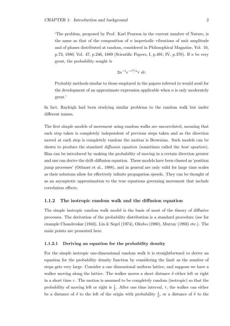
1.1 Plots showing P (x, t) for D = 1, 5 and 10, and t = 1 and 10. (The scales
on each plot are different). . . . . . . . . . . . . . . . . . . . . . . . . . . . . 4
1.2 Plots showing P (x, y, t) for D = 1 and 5, and t = 1 and 10. (The scales on
each plot are different). . . . . . . . . . . . . . . . . . . . . . . . . . . . . . 5
1.3 Plots of P (x, t), the solution of the drift diffusion equation, for various u . . 7
1.4 Plots of p(x, t), the solution of the telegraph equation for various parameter
values . . . . . . . . . . . . . . . . . . . . . . . . . . . . . . . . . . . . . . . 12
1.5 Example of a data set on a circle with R ≈ 0 but with a non-uniform spread
of points. . . . . . . . . . . . . . . . . . . . . . . . . . . . . . . . . . . . . . 15
1.6 Examples of the von Mises distribution for various values of κ, and µ = 0. . 16
1.7 Plot of κ against σ2. . . . . . . . . . . . . . . . . . . . . . . . . . . . . . . . 17
1.8 Plot comparing µ0(θ) for sinusoidal (—) and linear reorientation (- -), for
−π ≤ θ < π and B−1 = 0.1. . . . . . . . . . . . . . . . . . . . . . . . . . . . 28
2.1 Example of a two-dimensional lattice random walk. . . . . . . . . . . . . . . 32
2.2 Example of a multi-directional random walk. . . . . . . . . . . . . . . . . . 36
2.3 Plots showing f(x, y, t) for various parameter values at t = 10. . . . . . . . 43
3.1 Sketch of the probability distributions for h(δ) and k(θ) as used by Othmer
et al. (1988). . . . . . . . . . . . . . . . . . . . . . . . . . . . . . . . . . . . 51
3.2 Sketch showing the difference between D2 and σ2 (H is the average position). 52
3.3 Plots of Vx1(t) and Hx1(t) for various values of CI . . . . . . . . . . . . . . . 60
3.4 Plots of D2(t) and σ2(t) for various values of CI . . . . . . . . . . . . . . . . 61
4.1 Plot of V(t) for dτ = 0.1 and dτ = 0.3 and various values of κ. (The scale
of each plot is different) . . . . . . . . . . . . . . . . . . . . . . . . . . . . . 90
4.2 Plot of H(t) for dτ = 0.1 and dτ = 0.3 and various values of κ. (The scale
of each plot is different) . . . . . . . . . . . . . . . . . . . . . . . . . . . . . 90
4.3 Plot of D2(t) for dτ = 0.1 and dτ = 0.3 and various values of κ. (The scale
of each plot is different) . . . . . . . . . . . . . . . . . . . . . . . . . . . . . 91
4.4 Plot of σ2(t) for dτ = 0.1 and dτ = 0.3 and various values of κ. (The scale
of each plot is different) . . . . . . . . . . . . . . . . . . . . . . . . . . . . . 91
ix

x
4.5 Plot of D2x1(t) and D2
x2(t) for dτ = 0.3 and various values of κ. (The scale
of each plot is different) . . . . . . . . . . . . . . . . . . . . . . . . . . . . . 92
4.6 Plot of σ2x1(t) and σ2
x2(t) for dτ = 0.3 and various values of κ. (The scale of
each plot is different) . . . . . . . . . . . . . . . . . . . . . . . . . . . . . . . 92
4.7 Plot of ζ1 against κ for dτ = 0, 0.1, 0.2, 0.3. . . . . . . . . . . . . . . . . . . . 96
4.8 Plot of ζ2 against κ for dτ = 0.1, 0.2, 0.3. . . . . . . . . . . . . . . . . . . . . 97
5.1 Plots comparing k1(µ, κ) to the exact integral for various values of κ. (The
scale of each plot is different). . . . . . . . . . . . . . . . . . . . . . . . . . . 106
5.2 Plots comparing l1(µ, κ) to the exact integral for various values of κ. (The
scale of each plot is different). . . . . . . . . . . . . . . . . . . . . . . . . . . 107
5.3 Plots comparing m1(µ, κ) to the exact integral for various values of κ. (The
scale of each plot is different). . . . . . . . . . . . . . . . . . . . . . . . . . . 108
5.4 Plots comparing n1(µ, κ) to the exact integral for various values of κ. (The
scale of each plot is different). . . . . . . . . . . . . . . . . . . . . . . . . . . 109
5.5 Plots comparing k2(µ, κ) to the exact integral for various values of κ. (The
scale of each plot is different). . . . . . . . . . . . . . . . . . . . . . . . . . . 110
5.6 Plots comparing l2(µ, κ) to the exact integral for various values of κ. (The
scale of each plot is different). . . . . . . . . . . . . . . . . . . . . . . . . . . 111
5.7 Plots comparing m2(µ, κ) to the exact integral for various values of κ. (The
scale of each plot is different). . . . . . . . . . . . . . . . . . . . . . . . . . . 112
5.8 Plots comparing n2(µ, κ) to the exact integral for various values of κ. (The
scale of each plot is different). . . . . . . . . . . . . . . . . . . . . . . . . . . 113
5.9 Plot of V(t) for dτ = 0.1 and dτ = 0.3 and various values of κ. . . . . . . . 135
5.10 Plot of H(t) for dτ = 0.1 and dτ = 0.3 and various values of κ. . . . . . . . 135
5.11 Plot of D2(t) for dτ = 0.1 and dτ = 0.3 and various values of κ. (The scale
of each plot is different) . . . . . . . . . . . . . . . . . . . . . . . . . . . . . 136
5.12 Plot of σ2(t) for dτ = 0.1 and dτ = 0.3 and various values of κ. (The scale
of each plot is different) . . . . . . . . . . . . . . . . . . . . . . . . . . . . . 136
5.13 Plot of D2x1(t) and D2
x2(t) for dτ = 0.3 and various values of κ. (The scale
of each plot is different) . . . . . . . . . . . . . . . . . . . . . . . . . . . . . 137
5.14 Plot of σ2x1(t) and σ2
x2(t) for dτ = 0.3 and various values of κ. (The scale of
each plot is different) . . . . . . . . . . . . . . . . . . . . . . . . . . . . . . . 137
6.1 Simple algorithm for an individual random walk. . . . . . . . . . . . . . . . 143
6.2 i) Random walk with κ = 0.1, dτ = 0. The random walk is close to being
completely random (Brownian) motion. . . . . . . . . . . . . . . . . . . . . 145
6.3 ii) Random walk with κ = 2, dτ = 0. The random walk appears more
correlated but there is no overall preferred direction. . . . . . . . . . . . . . 146
xi
6.4 iii) Random walk with κ = 0.5, dτ = 0.2. The random walk is less correlated
but there is a definite preferred direction (y-direction). . . . . . . . . . . . . 146
6.5 iv) Random walk with κ = 4, dτ = 0.3. The random walk is highly corre-
lated and the preferred direction is clear. . . . . . . . . . . . . . . . . . . . . 147
6.6 Algorithm used to calculate average statistics for a set of random walks. . . 148
6.7 Plots showing theoretical Hy(t) (—), and 95% confidence interval from
simulated (· · ·), against time for sinusoidal reorientation with dτ = 0.1.
(The scale used for each plot is different.) . . . . . . . . . . . . . . . . . . . 152
6.8 Plots showing theoretical Hy(t) (—), and 95% confidence interval from
simulated (· · ·), against time for sinusoidal reorientation with dτ = 0.2.
(The scale used for each plot is different.) . . . . . . . . . . . . . . . . . . . 153
6.9 Plots showing theoretical Hy(t) (—), and 95% confidence interval from
simulated (· · ·), against time for sinusoidal reorientation with dτ = 0.3.
(The scale used for each plot is different.) . . . . . . . . . . . . . . . . . . . 154
6.10 Plots showing theoretical Hy(t) (—), and 95% confidence interval from
simulated (· · ·), against time for linear reorientation with dτ = 0.1. (The
scale used for each plot is different.) . . . . . . . . . . . . . . . . . . . . . . 156
6.11 Plots showing theoretical Hy(t) (—), and 95% confidence interval from
simulated (· · ·), against time for linear reorientation with dτ = 0.2. (The
scale used for each plot is different.) . . . . . . . . . . . . . . . . . . . . . . 157
6.12 Plots showing theoretical Hy(t) (—), and 95% confidence interval from
simulated (· · ·), against time for linear reorientation with dτ = 0.3. (The
scale used for each plot is different.) . . . . . . . . . . . . . . . . . . . . . . 158
6.13 Plots showing theoretical (—), and simulated (· · ·), absolute velocity (Hy(t)/t)
in the y-direction against time for sinusoidal reorientation with dτ = 0.1.
(The scale used for each plot is different.) . . . . . . . . . . . . . . . . . . . 160
6.14 Plots showing theoretical (—), and simulated (· · ·) absolute velocity (Hy(t)/t)
in the y-direction against time for sinusoidal reorientation with dτ = 0.3.
(The scale used for each plot is different.) . . . . . . . . . . . . . . . . . . . 161
6.15 Plots showing theoretical (—), and simulated (· · ·), absolute velocity (Hy(t)/t)
in the y-direction against time for linear reorientation with dτ = 0.1. (The
scale used for each plot is different.) . . . . . . . . . . . . . . . . . . . . . . 163
6.16 Plots showing theoretical (—), and simulated (· · ·), absolute velocity (Hy(t)/t)
in the y-direction against time for linear reorientation with dτ = 0.3. (The
scale used for each plot is different.) . . . . . . . . . . . . . . . . . . . . . . 164
6.17 Plots showing theoretical (—), and simulated (· · ·), D2(t) against time for
sinusoidal reorientation with dτ = 0.1. (The scale used for each plot is
different.) . . . . . . . . . . . . . . . . . . . . . . . . . . . . . . . . . . . . . 165

xii
6.18 Plots showing theoretical (—), and simulated (· · ·), D2(t) against time for
sinusoidal reorientation with dτ = 0.3. (The scale used for each plot is
different.) . . . . . . . . . . . . . . . . . . . . . . . . . . . . . . . . . . . . . 166
6.19 Plots showing theoretical (—), and simulated (· · ·), D2(t) against time for
linear reorientation with dτ = 0.1. (The scale used for each plot is different.)168
6.20 Plots showing theoretical (—), and simulated (· · ·), D2(t) against time for
linear reorientation with dτ = 0.3. (The scale used for each plot is different.)169
6.21 Plots showingD2x(t) andD2
y(t) against time for sinusoidal reorientation with
various values of the parameters. (The scale used for each plot is different.) 170
6.22 Plots showing D2x(t) and D2
y(t) against time for linear reorientation with
various values of the parameters. (The scale used for each plot is different.) 171
6.23 Plots showing theoretical (—), and simulated (· · ·), σ2(t) against time for
sinusoidal reorientation with dτ = 0. (The scale used for each plot is different.)173
6.24 Plots showing theoretical (—), and simulated (· · ·), σ2(t) against time for
sinusoidal reorientation with dτ = 0.1. (The scale used for each plot is
different.) . . . . . . . . . . . . . . . . . . . . . . . . . . . . . . . . . . . . . 174
6.25 Plots showing theoretical (—), and simulated (· · ·), σ2(t) against time for
sinusoidal reorientation with dτ = 0.2. (The scale used for each plot is
different.) . . . . . . . . . . . . . . . . . . . . . . . . . . . . . . . . . . . . . 175
6.26 Plots showing theoretical (—), and simulated (· · ·), σ2(t) against time for
sinusoidal reorientation with dτ = 0.3. (The scale used for each plot is
different.) . . . . . . . . . . . . . . . . . . . . . . . . . . . . . . . . . . . . . 176
6.27 Plots showing theoretical (—), and simulated (· · ·), σ2(t) against time for
linear reorientation with dτ = 0.1. (The scale used for each plot is different.)178
6.28 Plots showing theoretical (—), and simulated (· · ·), σ2(t) against time for
linear reorientation with dτ = 0.2. (The scale used for each plot is different.)179
6.29 Plots showing theoretical (—), and simulated (· · ·), σ2(t) against time for
linear reorientation with dτ = 0.3. (The scale used for each plot is different.)180
6.30 Plots showing σ2x(t) against time for sinusoidal reorientation with various
values of the parameters. (The scale used for each plot is different.) . . . . 181
6.31 Plots showing σ2y(t) against time for sinusoidal reorientation with various
values of the parameters. (The scale used for each plot is different.) . . . . 182
6.32 Plots showing σ2x(t) against time for linear reorientation with various values
of the parameters. (The scale used for each plot is different.) . . . . . . . . 183
6.33 Plots showing σ2y(t) against time for linear reorientation with various values
of the parameters. (The scale used for each plot is different.) . . . . . . . . 184
6.34 Example plots of the population position and spread at t = 100. . . . . . . 187
6.35 Plots showing Hy(100) against κ for sinusoidal and linear reorientation with
dτ = 0 (—), dτ = 0.1 (· · ·), dτ = 0.2 (−−) and dτ = 0.3 (· − ·). . . . . . . . 188

xiii
6.36 Plots showing D2(100) against κ for sinusoidal and linear reorientation with
dτ = 0 (—), dτ = 0.1 (· · ·), dτ = 0.2 (−−) and dτ = 0.3 (· − ·). . . . . . . . 189
6.37 Plots showing D2x(100) against κ for sinusoidal and linear reorientation with
dτ = 0 (—), dτ = 0.1 (· · ·), dτ = 0.2 (−−) and dτ = 0.3 (· − ·). . . . . . . . 190
6.38 Plots showing D2y(100) against κ for sinusoidal and linear reorientation with
dτ = 0 (—), dτ = 0.1 (· · ·), dτ = 0.2 (−−) and dτ = 0.3 (· − ·). . . . . . . . 192
6.39 Plots showing σ2(100) against κ for sinusoidal and linear reorientation with
dτ = 0 (—), dτ = 0.1 (· · ·), dτ = 0.2 (−−) and dτ = 0.3 (· − ·). . . . . . . . 193
6.40 Plots showing σ2y(100) against κ for sinusoidal and linear reorientation with
dτ = 0 (—), dτ = 0.1 (· · ·), dτ = 0.2 (−−) and dτ = 0.3 (· − ·). . . . . . . . 194
6.41 Plots showing (a) final position and spread (t = 100), (b) Hy(t), (c) σ2x(t)
and (d) σ2y(t) for reorientation parameters from data set C1:a. . . . . . . . . 197
6.42 Plots showing (a) final position and spread (t = 100), (b) Hy(t), (c) σ2x(t)
and (d) σ2y(t) for reorientation parameters from data set C1:b. . . . . . . . . 198
6.43 Plots showing (a) final position and spread (t = 100), (b) Hy(t), (c) σ2x(t)
and (d) σ2y(t) for reorientation parameters from data set C3:a. . . . . . . . . 200
6.44 Plots showing (a) final position and spread (t = 100), (b) Hy(t), (c) σ2x(t)
and (d) σ2y(t) for reorientation parameters from data set C3:b. . . . . . . . . 202
6.45 Plots showing (a) final position and spread (t = 100), (b) Hy(t), (c) σ2x(t)
and (d) σ2y(t) for reorientation parameters from data set C4:a. . . . . . . . . 203
6.46 Plots showing (a) final position and spread (t = 100), (b) Hy(t), (c) σ2x(t)
and (d) σ2y(t) for reorientation parameters from data set C4:b. . . . . . . . . 205
7.1 Plots of M0(t) against t. Legend: (- -) simulation κ = 1, (· · ·) simulation
κ = 2, (−·−) simulation κ = 4, (+) approximation κ = 1, (*) approximation
κ = 2, (♦) approximation κ = 4. . . . . . . . . . . . . . . . . . . . . . . . . 210
7.2 Plots showing theoretical and simulated long-time p.d.f., f(θ), with param-
eter values taken from Hill and Hader’s experiments with data set C1. . . . 211
7.3 Plots showing theoretical and simulated long-time p.d.f., f(θ), with param-
eter values taken from Hill and Hader’s experiments with data set C3. . . . 212
7.4 Plots showing theoretical and simulated long-time p.d.f., f(θ), with param-
eter values taken from Hill and Hader’s experiments with data set C4. . . . 213
7.5 Plots showing theoretical and simulated long-time p.d.f., f(θ), for data set
C1 with τ = 1. . . . . . . . . . . . . . . . . . . . . . . . . . . . . . . . . . . 214
7.6 Plots showing theoretical and simulated long-time p.d.f., f(θ), for data set
C4 with τ = 1. . . . . . . . . . . . . . . . . . . . . . . . . . . . . . . . . . . 214

xiv
7.7 Plots showing the first angular moment a1 against k0 for the sinusoidal re-
orientation model, with (a) B−1 = 0.1, (b) B−1 = 0.5. Legend: theoretical
results (—), simulation results with τ = 0.1 s (- -), simulation results with
τ = 1 s (· · ·). . . . . . . . . . . . . . . . . . . . . . . . . . . . . . . . . . . . 216
7.8 Plots showing the first angular moment a1 against k0 for the linear reori-
entation model, with (a) B−1 = 0.1, (b) B−1 = 0.5. Legend: theoretical
results (—), simulation results with τ = 0.1 s (- -), simulation results with
τ = 1 s (· · ·). . . . . . . . . . . . . . . . . . . . . . . . . . . . . . . . . . . . 216
7.9 Plots showing the third angular moment a3 against k0 with B−1 = 0.5, for
(a) sinusoidal reorientation model (b) linear reorientation model. Legend:
theoretical results (—), simulation results with τ = 0.1 s (- -), simulation
results with τ = 1 s (· · ·). . . . . . . . . . . . . . . . . . . . . . . . . . . . . 217
7.10 Plots showing the fourth angular moment a4 against k0 with B−1 = 0.5, for
(a) sinusoidal reorientation model (b) linear reorientation model. Legend:
theoretical results (—), simulation results with τ = 0.1 s (- -), simulation
results with τ = 1 s (· · ·). . . . . . . . . . . . . . . . . . . . . . . . . . . . . 218
7.11 Plots showing the effect of changing the sampling length τs of an individual
random walk. . . . . . . . . . . . . . . . . . . . . . . . . . . . . . . . . . . . 221
7.12 Plots showing how µδ(θ) changes with θ for the sinusoidal model with vari-
ous sampling lengths τs. Simulation results for angular bins of π9 rads (—),
and functions fitted by inspection to the data (- -). . . . . . . . . . . . . . . 222
7.13 Plots showing how σ2δ (θ) changes with θ for the sinusoidal model with vari-
ous sampling lengths τs. Simulation results for angular bins of π9 rads (—),
and the mean from the data averaging over all θ (- -). . . . . . . . . . . . . 223
7.14 Plots showing (a) the amplitude of the mean turning angle dτs , (b) vari-
ance of the turning angle σ2δ , against rescaled sampling length τs/τ for the
sinusoidal model. . . . . . . . . . . . . . . . . . . . . . . . . . . . . . . . . . 225
7.15 Plots showing how µδ(θ) changes with θ for the linear model with various
sampling lengths τs. Simulation results for angular bins of π9 rads (—), and
functions fitted by inspection to the data (- -). . . . . . . . . . . . . . . . . 227
7.16 Plots showing how σ2δ (θ) changes with θ for the linear model with various
sampling lengths τs. Simulation results for angular bins of π9 rads (—), and
the mean from the data averaging over all θ (- -). . . . . . . . . . . . . . . . 228
7.17 Plots showing (a) the amplitude of the mean turning angle dτs , (b) variance
of the turning angle σ2δ , against rescaled sampling length τs/τ for the linear
model. . . . . . . . . . . . . . . . . . . . . . . . . . . . . . . . . . . . . . . . 229
7.18 Plots showing how µδ(θ) and σ2δ change with θ for the sinusoidal model
with fixed time between turns. . . . . . . . . . . . . . . . . . . . . . . . . . 231

xv
7.19 Plots showing how µδ(θ) and σ2δ change with θ for the linear model with
fixed time between turns. . . . . . . . . . . . . . . . . . . . . . . . . . . . . 232
7.20 Plots showing (a) the amplitude of the mean turning angle dτs , (b) vari-
ance of the turning angle σ2δ , against rescaled sampling length τs/τ for the
sinusoidal model with fixed time between turns. . . . . . . . . . . . . . . . . 233
7.21 Plots showing (a) the amplitude of the mean turning angle dτs , (b) variance
of the turning angle σ2δ , against rescaled sampling length τs/τ for the linear
model with fixed time between turns. . . . . . . . . . . . . . . . . . . . . . . 233
7.22 Log-plot of − log10(τ) against ρ. . . . . . . . . . . . . . . . . . . . . . . . . 236
8.1 Plots showing Hy(100) against κ for sinusoidal and linear reorientation for
dτ = 0.1 (—), and dτ = 0.3 (· · ·). . . . . . . . . . . . . . . . . . . . . . . . . 240
8.2 Plots showing σ2x(100) against κ for sinusoidal and linear reorientation for
dτ = 0.1 (—), and dτ = 0.3 (· · ·). . . . . . . . . . . . . . . . . . . . . . . . . 241
8.3 Plots showing σ2y(100) against κ for sinusoidal and linear reorientation for
dτ = 0.1 (—), and dτ = 0.3 (· · ·). . . . . . . . . . . . . . . . . . . . . . . . . 242
8.4 Plots showing distribution at t = 100 for sinusoidal and linear reorientation
for dτ = 0.1 and κ = 0.1, κ = 10 and κ = 50. . . . . . . . . . . . . . . . . . 243
8.5 Plots showing Hy(100) against dτ for sinusoidal and linear reorientation for
κ = 1 (—), and κ = 4 (· · ·). . . . . . . . . . . . . . . . . . . . . . . . . . . . 244
8.6 Plots showing σ2x(100) against dτ for sinusoidal and linear reorientation for
κ = 1 (—), and κ = 4 (· · ·). . . . . . . . . . . . . . . . . . . . . . . . . . . . 245
8.7 Plots showing σ2y(100) against dτ for sinusoidal and linear reorientation for
κ = 1 (—), and κ = 4 (· · ·). . . . . . . . . . . . . . . . . . . . . . . . . . . . 245
8.8 Plots showing distribution at t = 100 for sinusoidal and linear reorientation
for κ = 4 and dτ = 0.1, dτ = 1 and dτ = 2. . . . . . . . . . . . . . . . . . . . 247
8.9 Plot of dopt against κ for sinusoidal reorientation. . . . . . . . . . . . . . . . 249
8.10 Plot of κ(y) against y with κI = 1, for p = 0.01 (—), p = 0.05 (· · ·), and
p = 0.1 (- -). . . . . . . . . . . . . . . . . . . . . . . . . . . . . . . . . . . . . 252
8.11 Plots showing individual random walks for sinusoidal reorientation with
κ(y) for various parameter values. (The scale of each plot is different) . . . 253
8.12 Plots showing Hy(100) against p for sinusoidal and linear reorientation for
dτ = 0.1 (—), and dτ = 0.3 (· · ·). . . . . . . . . . . . . . . . . . . . . . . . . 254
8.13 Plots showing σ2x(100) against p for sinusoidal and linear reorientation for
dτ = 0.1 (—), and dτ = 0.3 (· · ·). . . . . . . . . . . . . . . . . . . . . . . . . 255
8.14 Plots showing σ2y(100) against p for sinusoidal and linear reorientation for
dτ = 0.1 (—), and dτ = 0.3 (· · ·). . . . . . . . . . . . . . . . . . . . . . . . . 255
8.15 Plots showing distribution at t = 100 for sinusoidal and linear reorientation
for dτ = 0.1 and p = 0.05 and p = 0.5. . . . . . . . . . . . . . . . . . . . . . 257

xvi
8.16 Plot of dτ (y) against y with dint = 0.1 and dopt = 1, for q = 0.01 (—),
q = 0.05 (· · ·), and q = 0.1 (- -). . . . . . . . . . . . . . . . . . . . . . . . . 258
8.17 Plots showing individual random walks for sinusoidal reorientation with
dτ (y) for various parameter values. (The scale of each plot is different) . . . 259
8.18 Plots showing Hy(100) against q for sinusoidal and linear reorientation for
κ = 1 (—), and κ = 4 (· · ·). . . . . . . . . . . . . . . . . . . . . . . . . . . . 260
8.19 Plots showing σ2x(100) against q for sinusoidal and linear reorientation for
κ = 1 (—), and κ = 4 (· · ·). . . . . . . . . . . . . . . . . . . . . . . . . . . . 261
8.20 Plots showing σ2y(100) against q for sinusoidal and linear reorientation for
κ = 1 (—), and κ = 4 (· · ·). . . . . . . . . . . . . . . . . . . . . . . . . . . . 261
8.21 Plots showing distribution at t = 100 for sinusoidal and linear reorientation
for κ = 4 and q = 0.01 and q = 0.1. . . . . . . . . . . . . . . . . . . . . . . . 263
8.22 Plots showing individual random walks for sinusoidal and linear reorienta-
tion where the preferred direction is to a point. . . . . . . . . . . . . . . . . 265
8.23 Plots showing the average position in the y-direction, Hy(t), against t for
sinusoidal and linear reorientation. . . . . . . . . . . . . . . . . . . . . . . . 266
8.24 Plots showing the spread in the x-direction, σ2x(t), against t for sinusoidal
and linear reorientation. . . . . . . . . . . . . . . . . . . . . . . . . . . . . . 268
8.25 Plots showing the spread in the y-direction, σ2y(t), against t for sinusoidal
and linear reorientation. . . . . . . . . . . . . . . . . . . . . . . . . . . . . . 269
8.26 Plots showing distribution at t = 100 for sinusoidal and linear reorientation
where the preferred direction is to a point. . . . . . . . . . . . . . . . . . . . 270
9.1 Plots of the spread of a population of 500 walkers after t = 100, moving
as an unbiased and correlated velocity jump process with (a) κ = 1, (b)
κ = 50. The dotted circle shows the maximum possible displacement at
t = 100. . . . . . . . . . . . . . . . . . . . . . . . . . . . . . . . . . . . . . . 278
9.2 Plots comparing expected values of Z(c, t) (—) to simulated results (+) for
(a) κ = 1, (b) κ = 4, (c) κ = 10, (d) κ = 20. . . . . . . . . . . . . . . . . . . 281
9.3 Plots of MDD(t) v t for the velocity jump process model (—), Kareiva &
Shigesada’s model (· · ·), Bovet & Benhamou’s model (- -), and simulation
results (+). . . . . . . . . . . . . . . . . . . . . . . . . . . . . . . . . . . . . 282
9.4 Plots of MDD(t) v t for velocity jump process model with Z(c, t) (—),
Z = 0.89 (- -), and simulation results (+). . . . . . . . . . . . . . . . . . . . 283
9.5 Simulated plots of the spread of a population of 500 walkers after t = 100,
moving as a biased and correlated velocity jump process with dτ = 0.1 and
(a) sinusoidal reorientation, κ = 1, (b) sinusoidal reorientation, κ = 50, (c)
linear reorientation, κ = 1, (d) linear reorientation, κ = 50. . . . . . . . . . 285

xvii
9.6 Plots of values of Z(κ, dτ , t), Zx(κ, dτ , t), and Zy(κ, dτ , t) as a function of κ
at t = 1000 from numerical simulations of sinusoidal and linear reorientation
with dτ = 0.1 (- -), dτ = 0.5 (· · ·), and dτ = 1 (- · -). The solid lines (—)
correspond to Z = 0.798 or Z = 0.89 respectively, the expected values if
the distribution is Normal. . . . . . . . . . . . . . . . . . . . . . . . . . . . . 287
10.1 Simple ‘infinite’ reef model. . . . . . . . . . . . . . . . . . . . . . . . . . . . 295
10.2 Plots showing (a) survival probability PR(VF , γ) against death rate for (a)
0.0001 ≤ µ ≤ 0.0002, and (b) 0.0002 ≤ µ ≤ 0.0004. Legend: deterministic
model (—), stochastic model (- -), simulation model (+). . . . . . . . . . . 298
10.3 Plots of relative survival probability RSP against PR(VF , 0) from theoreti-
cal (—) and simulation (+) results. . . . . . . . . . . . . . . . . . . . . . . . 299
10.4 Simple circular reef model. . . . . . . . . . . . . . . . . . . . . . . . . . . . . 301
10.5 Plots showing survival probability PR(dτ , κ) for sinusoidal reorientation and
Model 2 against (a) κ, for dτ = 0.1 (—), dτ = 0.3 (- -), dτ = 0.5 (· · ·), and
dτ = 1.0 (- · -); (b) dτ , for κ = 0.4 (—), κ = 1.0 (- -), κ = 2.0 (· · ·), and
κ = 4.0 (- · -). . . . . . . . . . . . . . . . . . . . . . . . . . . . . . . . . . . . 302
10.6 Plots showing survival probability PR(dτ , κ) for linear reorientation and
Model 2 against (a) κ, for dτ = 0.1 (—), dτ = 0.3 (- -), dτ = 0.5 (· · ·), and
dτ = 1.0 (- · -); (b) dτ , for κ = 0.4 (—), κ = 1.0 (- -), κ = 2.0 (· · ·), and
κ = 4.0 (- · -). . . . . . . . . . . . . . . . . . . . . . . . . . . . . . . . . . . . 302
10.7 Circular reef with a constant current. . . . . . . . . . . . . . . . . . . . . . . 304
10.8 Plots showing survival probability PR(dτ , κ) for sinusoidal reorientation and
Model 3 against (a) κ, for dτ = 0.2 (—), dτ = 0.5 (- -), dτ = 1.0 (· · ·), and
dτ = 1.5 (- · -); (b) dτ , for κ = 1.8 (—), κ = 2.0 (- -), κ = 3.0 (· · ·), and
κ = 5.0 (- · -). . . . . . . . . . . . . . . . . . . . . . . . . . . . . . . . . . . . 305
10.9 Plots showing survival probability PR(dτ , κ) for linear reorientation and
Model 3 against (a) κ, for dτ = 0.1 (—), dτ = 0.3 (- -), dτ = 0.5 (· · ·), and
dτ = 1.0 (- · -); (b) dτ , for κ = 1.4 (—), κ = 2.0 (- -), κ = 3.0 (· · ·), and
κ = 5.0 (- · -). . . . . . . . . . . . . . . . . . . . . . . . . . . . . . . . . . . . 306
10.10Plots showing survival probability PR(U, κ) v U with dτ = 0.8 for (a) si-
nusoidal reorientation and (b) linear reorientation. Legend: κ = 1.0 (—),
κ = 2.0 (- -), κ = 3.0 (· · ·), and κ = 5.0 (- · -). . . . . . . . . . . . . . . . . . 306

List of Tables
1.1 Swimming speed and reorientation parameters estimated by Hill & Hader
for the data sets C1, C3 and C4. . . . . . . . . . . . . . . . . . . . . . . . . 29
5.1 Long-time numerical solutions for V(t) with linear reorientation . . . . . . . 133
5.2 Long-time numerical solutions for D2x1(t) with linear reorientation . . . . . 134
5.3 Long-time numerical solutions for D2x2(t) with linear reorientation . . . . . 134
5.4 Long-time numerical solutions for σ2x1(t) with linear reorientation . . . . . . 134
5.5 Comparing long-time numerical solutions for H(t) . . . . . . . . . . . . . . 139
5.6 Comparing long-time numerical solutions for σ2(t) . . . . . . . . . . . . . . 140
7.1 Estimated value for the amplitude of the mean turning angle µδ(θ), and
calculated mean value of σ2δ , for the sinusoidal model with rescaled sampling
length τs/τ . . . . . . . . . . . . . . . . . . . . . . . . . . . . . . . . . . . . . 224
7.2 Estimated value for the amplitude of the mean turning angle µδ(θ), and
calculated mean value of σ2δ , for the linear model with rescaled sampling
length τs/τ . . . . . . . . . . . . . . . . . . . . . . . . . . . . . . . . . . . . . 227
7.3 Estimated value for the amplitude of the mean turning angle µδ(θ), and cal-
culated mean value of σ2δ , for the sinusoidal model with fixed time between
turns and with rescaled sampling length τs/τ . . . . . . . . . . . . . . . . . . 231
7.4 Estimated value for the amplitude of the mean turning angle µδ(θ), and
calculated mean value of σ2δ , for the linear model with fixed time between
turns and with rescaled sampling length τs/τ . . . . . . . . . . . . . . . . . . 232
7.5 Values of ρ, the ratio between the expected and observed values of B−1 with
the corresponding average time step between turns in the original random
walk, τ . . . . . . . . . . . . . . . . . . . . . . . . . . . . . . . . . . . . . . . 236
xviii

Chapter 1
Introduction and background
1.1 General background to random walks
1.1.1 History
1.1.1.1 Brownian motion
The endless irregular motion of individual pollen particles in liquid was famously studied
by the English botanist Brown (1828), and such random movement has been subsequently
known as Brownian motion. At the turn of the century many eminent physicists such
as Einstein (1905, 1906) and Smoluchowski (1916) were drawn to the subject. During
the course of research on Brownian motion, not only random walk theory (Uhlenbeck
& Ornstein, 1930), but also such important fields as random processes, random noise,
spectral analysis, and stochastic equations were developed.
1.1.1.2 The random walk
Classical works on probability have been in existence for centuries so it is somewhat
surprising that the first ‘random walk’ problem only appeared in the literature in 1905
when the journal Nature (Vol. 72, p.294) published ‘The problem of the random walker’
by Karl Pearson. The question posed was this:
‘A man starts from a point 0 and walks l yards in a straight line: he then turns
through any angle whatever and walks another l yards in a second straight line. He
repeats this process n times. I require the probability that after these n stretches
he is at a distance between r and r + δr from his starting point 0. The problem is
one of considerable interest, but I have only succeeded in obtaining an integrated
solution for two stretches. I think, however, that a solution ought to be found, if
only in the form of a series in powers of 1/n, where n is large.’
Lord Rayleigh responded (Nature, Vol. 72, p.318, 1905):
1
CHAPTER 1: Introduction and background 2
‘The problem, proposed by Prof. Karl Pearson in the current number of Nature, is
the same as that of the composition of n isoperiodic vibrations of unit amplitude
and of phases distributed at random, considered in Philosophical Magazine, Vol. 10,
p.73, 1880; Vol. 47, p.246, 1889 (Scientific Papers, I, p.491; IV, p.370). If n be very
great, the probability sought is
2n−1e−r2/nr dr.
Probably methods similar to those employed in the papers referred to would avail for
the development of an approximate expression applicable when n is only moderately
great.’
In fact, Rayleigh had been studying similar problems to the random walk but under
different names.
The first simple models of movement using random walks are uncorrelated, meaning that
each step taken is completely independent of previous steps taken and as the direction
moved at each step is completely random the motion is Brownian. Such models can be
shown to produce the standard diffusion equation (sometimes called the heat equation).
Bias can be introduced by making the probability of moving in a certain direction greater
and one can derive the drift-diffusion equation. These models have been classed as ‘position
jump processes’ (Othmer et al., 1988), and in general are only valid for large time scales
as their solutions allow for effectively infinite propagation speeds. They can be thought of
as an asymptotic approximation to the true equations governing movement that include
correlation effects.
1.1.2 The isotropic random walk and the diffusion equation
The simple isotropic random walk model is the basis of most of the theory of diffusive
processes. The derivation of the probability distribution is a standard procedure (see for
example Chandreskar (1943), Lin & Segel (1974), Okubo (1980), Murray (1993) etc.). The
main points are presented here.
1.1.2.1 Deriving an equation for the probability density
For the simple isotropic one-dimensional random walk it is straightforward to derive an
equation for the probability density function by considering the limit as the number of
steps gets very large. Consider a one dimensional uniform lattice, and suppose we have a
walker moving along the lattice. The walker moves a short distance δ either left or right
in a short time τ . The motion is assumed to be completely random (isotropic) so that the
probability of moving left or right is 12 . After one time interval, τ , the walker can either
be a distance of δ to the left of the origin with probability 12 , or a distance of δ to the

CHAPTER 1: Introduction and background 3
right of the origin with probability 12 . After the next time interval, the walker will either
be a distance of 2δ to the left of the origin with probability 14 , or a distance of 2δ to the
right of the origin with probability 14 , or will have returned to the origin with probability
12 (but the walker cannot still be a distance δ from the origin — the walker can only be
an even distance from the origin). Continuing in this way, the probability that a walker
will be at a distance of mδ to the right of the origin after N time steps (where m and N
are even), is given by
p(m,N) = (1
2)N
N !
[(N +m)/2]![(N −m)/2]!= (
1
2)N
NN−m
2
. (1.1)
This is the binomial distribution, which for large N converges to the Gaussian (or Normal)
distribution, see for example Clarke & Cooke (1992). Thus,
limN→∞
p(m,N) =
(
2
πN
) 1
2
e−m2/2N . (1.2)
Let x = mδ, and t = τN , and since m is even we set
P (x, t) dx ≡ p
(
x
δ,t
τ
)
dx
2δ. (1.3)
Then the probability of being between x and x+ dx is given by
P (x, t) dx =1
√
2πδ2t/τe−x
2τ/2δ2t dx, (1.4)
and if we take limits such that τ, δ → 0, while δ2/τ = constant ≡ 2D, then
P (x, t) =1√
4πDte−x
2/4Dt. (1.5)
For x ∈ R and t ∈ R+, equation (1.5) is the fundamental solution to the diffusion equation
∂P
∂t= D
∂2P
∂2x, (1.6)
where P (x, 0) = δ(x) (where δ is the Dirac delta function). If we multiply equation (1.6)
by N , the number of individual walkers in a population, then we get a special case (where
D is constant) of Fick’s equation (1.7) for the concentration (C), or number density of the
population (see Okubo (1980))
∂C
∂t=
∂
∂x
(
D∂C
∂x
)
. (1.7)
Solution plots for (1.5) are shown in Figure 1.1.
Useful statistics of this process are the mean position, < x >, and the mean squared
displacement, < x2 >, defined as
< x >=
∫
∞
−∞
xP (x, t) dx, (1.8)
CHAPTER 1: Introduction and background 4
D=1D=5D=10
0
0.05
0.1
0.15
0.2
0.25
P(x,t)
–40 –20 20 40x
(a) P (x, 1)
D=1D=5D=10
0
0.02
0.04
0.06
0.08
P(x,t)
–40 –20 20 40x
(b) P (x, 10)
Figure 1.1: Plots showing P (x, t) for D = 1, 5 and 10, and t = 1 and 10. (The scales on
each plot are different).
and
< x2 >=
∫
∞
−∞
x2P (x, t) dx. (1.9)
For the one-dimensional diffusion solution, < x >= 0 (as we have no bias or preferred
direction), and < x2 >= 2Dt. It is a standard result for a diffusion process that the mean
squared displacement increases in proportion to time, < x2 >∼ t.
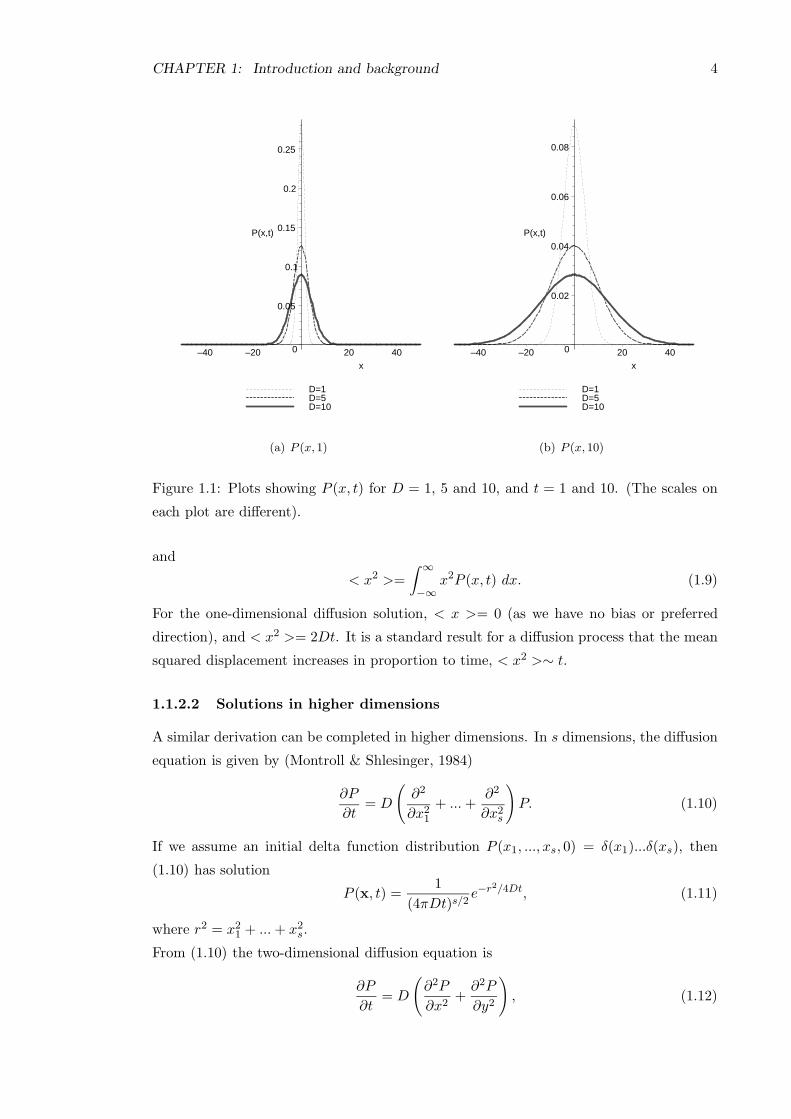
1.1.2.2 Solutions in higher dimensions
A similar derivation can be completed in higher dimensions. In s dimensions, the diffusion
equation is given by (Montroll & Shlesinger, 1984)
∂P
∂t= D
(
∂2
∂x21
+ ...+∂2
∂x2s
)
P. (1.10)
If we assume an initial delta function distribution P (x1, ..., xs, 0) = δ(x1)...δ(xs), then
(1.10) has solution
P (x, t) =1
(4πDt)s/2e−r
2/4Dt, (1.11)
where r2 = x21 + ...+ x2
s.
From (1.10) the two-dimensional diffusion equation is
∂P
∂t= D
(
∂2P
∂x2+∂2P
∂y2
)
, (1.12)

CHAPTER 1: Introduction and background 5
where P (x, y, 0) = δ(x)δ(y). From (1.11), the solution is
P (x, y, t) =1
4πDte−(x2+y2)/4Dt. (1.13)
Plots of example solutions for (1.13) are shown in Figure 1.2 for different diffusion coeffi-
cients, D.
–20
–10
0
10
20
x
–20
–10
0
10
20
y
0
0.02
0.04
0.06
0.08
P(x,y,t)
(a) P (x, y, 1) for D = 1
–20
–10
0
10
20
x
–20
–10
0
10
20
y
0
0.002
0.004
0.006
0.008
P(x,y,t)
(b) P (x, y, 10) for D = 1
–20
–10
0
10
20
x
–20
–10
0
10
20
y
0
0.002
0.004
0.006
0.008
0.01
0.012
0.014
0.016
P(x,y,t)
(c) P (x, y, 1) for D = 5
–20
–10
0
10
20
x
–20
–10
0
10
20
y
0
0.0002
0.0004
0.0006
0.0008
0.001
0.0012
0.0014
0.0016
P(x,y,t)
(d) P (x, y, 10) for D = 5
Figure 1.2: Plots showing P (x, y, t) for D = 1 and 5, and t = 1 and 10. (The scales on
each plot are different).
For the two-dimensional diffusion solution, the mean position is < (x, y) >= (0, 0) , and
the mean squared displacement is < r2 >=< (x2 + y2) >= 4Dt.
Looking at the solutions in (1.5) and (1.13), one can see that P (x, t) > 0 for any t > 0
and any x, y ∈ R. The diffusion process predicts a non-zero probability for arbitrarily
large displacements at arbitrarily small times, and in this sense the underlying speed
of propagation is infinite. Because of this, and because in (1.2) and (1.5) we assumed
that N → ∞ and δ → 0, the solution of the diffusion equation can be considered as an

CHAPTER 1: Introduction and background 6
asymptotic approximation, valid for large time, of equations that more accurately describe
the correlations in movement that are likely to be present at shorter time scales.
1.1.2.3 Using a difference equation to derive the diffusion equation
In the previous section, we showed how to derive an equation for the solution to the
diffusion equation P (x, t) directly. Working the other way, it is possible to set up a
difference equation and then derive the diffusion equation by completing a Taylor series
expansion and taking appropriate limits, see for example Lin & Segel (1974), Okubo
(1980) etc. With this method it is easy to introduce different probabilities for left and
right movement, and derive a form of the diffusion equation that includes drift.
Consider a walker moving along a one-dimensional lattice, where at each time step τ it
either moves a distance δ to the left with probability l, or a distance δ to the right with
probability r, or stays in the same position with probability 1−r− l (the isotropic random
walk has r = l = 1/2). We define the probability that an individual walker is at a position
x at time t by P (x, t). One time step earlier, at time t− τ , the walker must have been at
position x − δ and then moved to the right, or at position x + δ and then moved to the
left, or at position x and then not moved at all. Thus
P (x, t) = P (x, t− τ)(1 − l − r) + P (x− δ, t− τ)r + P (x+ δ, t− τ)l. (1.14)
We now assume that τ and δ are small when compared to t and x respectively, so that
(1.14) can be expanded as a Taylor series in x and t. Writing P for P (x, t), we have
P =
(
P − τ∂P
∂t
)
(1 − l − r) +
(
(P − τ∂P
∂t− δ
∂P
∂x+δ2
2
∂2P
∂2x
)
r
+
(
(P − τ∂P
∂t+ δ
∂P
∂x+δ2
2
∂2P
∂2x
)
l +O(δ3) +O(τ2). (1.15)
Rearranging this gives
∂P
∂t= −δǫ
τ
∂P
∂x+kδ2
2τ
∂2P
∂x2+O(δ3) +O(τ2), (1.16)
where ǫ = r − l and k = l + r. We now let δ, τ, ǫ → 0 in such a way that the following
limits are finite:
u = limδ,ǫ,τ→0
δǫ
τ, (1.17)
D = k limδ,ǫ,τ→0
δ2
2τ. (1.18)
Taking these limits, the O(δ3) and O(τ2) terms in (1.16) go to zero yielding
∂P
∂t= −u∂P
∂x+D
∂2P
∂x2. (1.19)

CHAPTER 1: Introduction and background 7
This is a form of the diffusion equation that includes drift. Note that if we set r = l = 1/2
as in the isotropic random walk, then u = 0, giving (1.6).
The fact that we have introduced waiting into the random walk by allowing a walker to
stay in the same position (with probability 1 − r − l), does not change the final diffusion
equation solution. However, from (1.18) one can see that k = l + r < 1 in this case, and
hence the value of the diffusion constant D will be smaller.
For x ∈ R and t ∈ R+, Montroll & Shlesinger (1984) give the solution that satisfies (1.19)
with initial condition P (x, 0) = δ(x) as
P (x, t) =1√
4πDte−(x−ut)2/4Dt. (1.20)
Solution plots for (1.20) are shown in Figure 1.3.
t=1t=10t=50
0.05
0.1
0.15
0.2
0.25
P(x,t)
–20 20 40 60 80 100 120x
(a) P (x, t) with D = 1, u = 1
t=1t=10t=50
0.05
0.1
0.15
0.2
0.25
P(x,t)
–20 20 40 60 80 100 120x
(b) P (x, t) with D = 1, u = 2
Figure 1.3: Plots of P (x, t), the solution of the drift diffusion equation, for various u
Similar derivations can be completed for two-dimensional random walks, and results are
presented in Chapter 2.
It is possible to calculate the statistics < x > and < x2 > directly from the drift-diffusion
equation without having to solve to find P (x, t). This is a technique that we will exploit
in later chapters. To find < x >, multiply (1.19) by x and integrate over R to give
∫
∞
−∞
x∂P
∂tdx = −u
∫
∞
−∞
x∂P
∂xdx+D
∫
∞
−∞
x∂2P
∂t2dx. (1.21)
Using integration by parts and making the assumption that P (x, t) and its first two x
derivatives tend to zero as |x| → ∞ gives
d < x >
dt= u, (1.22)

CHAPTER 1: Introduction and background 8
which with the initial condition < x > (0) = 0, has solution
< x > (t) = ut. (1.23)
In a similar manner we can derive a differential equation for < x2 >,
d < x2 >
dt= 2u2t+ 2D, (1.24)
which with the initial condition < x2 > (0) = 0, has solution
< x2 > (t) = u2t2 + 2Dt. (1.25)
The same solutions can be obtained by multiplying (1.20) by x or x2 and then integrating
over R. The statistic
σ2(t) =
∫
∞
−∞
[x− < x >]2P (x, t) dx, (1.26)
that measures the dispersal about the mean position, is more appropriate for a diffusion
drift process than < x2 >, which measures the dispersal about the origin. For (1.19),
σ2(t) = 2Dt, the same value as < x2 > for a diffusion process without drift.
The limiting process in (1.18) is such that terms of the form δ2/τ tend to be finite as
δ, τ → 0, which means that δ/τ → ∞ as δ, τ → 0, implying an infinite propagation
speed, see Okubo (1980). Othmer et al. (1988) classified this way of modelling movement
using an uncorrelated random walk as a ‘position jump process’.
1.1.3 Random walks to a barrier — a simple example
Using the simple random walk models described above it is possible to investigate the
effect of placing a barrier into the random walk. To model movement in a confined domain
(for example fish swimming in a tank), then one can impose a ‘repelling’ or ‘reflecting’
barrier — a walker reaching the barrier will turn around and move away in the opposite
direction. To model movement where walkers leave the system upon reaching a given
point (for example larval fish recruiting to a reef — see Chapter 10), then one can impose
an ‘absorbing’ barrier — a walker reaching the barrier will be absorbed and is no longer
part of the system. The following simple example of an absorbing barrier is adapted from
an example in Grimmett & Stirzaker (2001).
Suppose we have a random walk process that satisfies the diffusion equation with drift
(1.19), i.e. we have∂g
∂t= −u∂g
∂x+σ2
2
∂2g
∂x2x > 0, (1.27)
where g is the probability density, u is the drift in the x direction, and σ2 is the variance
about the x position. Suppose the walker starts at position x = d > 0, and we have an
‘absorbing barrier’ at x = 0 — if a walker reaches the point x = 0 it is ‘absorbed’ and

CHAPTER 1: Introduction and background 9
removed from the system. This gives the boundary conditions
g(t, 0) = 0 t ≥ 0, (1.28)
g(0, x) = δ(x− d) x ≥ 0. (1.29)
From (1.20), the solution to (1.27) with boundary condition (1.29) is
g(t, x) =1
σ√
2πtexp
(
−(x− d− ut)2
2σ2t
)
. (1.30)
From Grimmett & Stirzaker (2001), the solution to (1.27) that takes into account both
boundary conditions (1.28) and (1.29) is
g(t, x) =1
σ√
2πt
[
exp
(
−(x− d− ut)2
2σ2t
)
− exp
(
−(x+ d− ut)2
2σ2t− 2ud
σ2
)]
. (1.31)
It is a simple step to derive the density function of the time ta until the absorption of the
walker. At time t, either the walker has been absorbed, or its position has density function
given by (1.31), and hence
P (ta ≤ t) = 1 −∫
∞
0g(t, x)dx. (1.32)
Differentiation with respect to t of the cumulative distribution in (1.32) gives the proba-
bility density function fa(t) of the absorbing time ta,
fa(t) =d
σ√
2πt3exp
(
−(d+ ut)2
2σ2t
)
. (1.33)
The probability of absorption taking place (ta <∞) is given by
P (ta <∞) =
1 if u ≤ 0
e−2ud if u > 0.(1.34)
1.1.4 The telegraph equation
In the previous section we derived diffusion equations as the governing equations behind
the spatial distribution of a simple random walk. The random walks did not include
correlation — the direction of motion chosen at a certain step was independent of the
previous direction of movement. As a consequence, solutions of the diffusion equation can
have infinite propagation speed. The solutions are satisfactory for large time-scales but
for smaller time-scales we must look for a better model that includes correlation effects.
The one-dimensional telegraph equation was first derived by Goldstein (1951), (see also
Kac (1974), Okubo (1980), Othmer et. al (1988), etc), and we present the derivation here.

CHAPTER 1: Introduction and background 10
1.1.4.1 The unbiased one-dimensional telegraph equation
We restrict the population to moving left or right along an infinite line at a constant speed
v. We split the population into left-moving individuals β and right-moving individuals α,
where the total population is given by p = α + β. At each time step τ the individuals
either move a distance δ in the direction they were previously moving (with a probability
given by q = 1 − λτ) or they change direction and then move a distance δ in this new
direction (with the turning probability given by r = λτ).
If we take a forward time step then the number density of individuals at position x moving
right and left respectively is given by
α(x, t+ τ) = qα(x− δ, t) + rβ(x− δ, t),
β(x, t+ τ) = rα(x+ δ, t) + qβ(x+ δ, t).
We can expand these equations as Taylor series to give
α+ τ∂α
∂t+O(τ2) = q(α− δ
∂α
∂x+O(δ2)) + r(β − δ
∂β
∂x+O(δ2)),
β + τ∂β
∂t+O(τ2) = q(β + δ
∂β
∂x+O(δ2)) + r(α+ δ
∂α
∂x+O(δ2)).
Substituting for q and r gives
α+ τ∂α
∂t+O(τ2) = α− δ
∂α
∂x− λτα+ λτδ
∂α
∂x+ λτβ − λτδ
∂β
∂x+O(δ2),
β + τ∂β
∂t+O(τ2) = β + δ
∂β
∂x− λτβ − λτδ
∂β
∂x+ λτα+ λτδ
∂α
∂x+O(δ2).
Now divide through by τ and take the limit such that δ/τ → v as δ → 0 and τ → 0 (where
v is the constant speed), giving
∂α
∂t= −v∂α
∂x+ λ(β − α), (1.35)
∂β
∂t= v
∂β
∂x− λ(β − α). (1.36)
Adding (1.35) and (1.36) gives
∂(α + β)
∂t= v
∂(β − α)
∂x, (1.37)
which can be differentiated to give
∂2(α+ β)
∂t2= v
∂2(β − α)
∂x∂t. (1.38)
Subtracting (1.36) from (1.35) gives
∂(β − α)
∂t= v
∂(α + β)
∂x− 2λ(β − α), (1.39)
which can be differentiated to give
∂2(β − α)
∂x∂t= v
∂2(α+ β)
∂x2− 2λ
∂(β − α)
∂x. (1.40)

CHAPTER 1: Introduction and background 11
Substituting (1.40) into (1.38), and using (1.37) and the fact that α+ β = p, gives
∂2p
∂t2+ 2λ
∂p
∂t= v2 ∂
2p
∂x2. (1.41)
This is the telegraph equation. The equation can be solved if given initial conditions
specified by the initial distribution p(x, 0). We have a fixed speed v and so (unlike the
diffusion equation) we cannot have an arbitrarily large propagation speed.
Multiplying (1.41) by x, and integrating over R gives the mean < x >, which for the
unbiased telegraph equation is zero. Multiplying (1.41) by x2, and integrating over R
gives a differential equation for the mean squared displacement < x2 > ,
d2 < x2 >
dt2+ 2λ
d < x2 >
dt= 2s2. (1.42)
Assuming that p(x, 0) = δ(x) and ∂p∂t (x, 0) = 0, then the appropriate initial conditions for
(1.42) are < x2(0) >= ddt < x2(0) >= 0, and the solution is
< x2(t) >=v2
λ
(
t− 1
2λ(1 − e−2λt)
)
. (1.43)
For small t, < x2(t) >∼ v2t2, which is characteristic of a wave propagation process, and
for large t, < x2(t) >∼ v2t/λ, which is characteristic of a diffusion process with diffusion
coefficient D = v2/2λ.
When deriving the uncorrelated random walk we showed that D = δ2/2τ , and these two
results can be related. In a Poisson process of intensity λ the mean time between events
is 1/λ, see Grimmett & Stirzaker (2001). Thus the average distance travelled between
reversals is δ = v/λ, and therefore
D =v2
2λ=δ2λ
2. (1.44)
Since τ = 1/λ, the ‘diffusion limit’ of the telegraph process consists of letting λ → ∞(equivalent to τ → 0 for uncorrelated process), and v → ∞ (equivalent to δ/τ → ∞for uncorrelated process), while maintaining v2/λ constant (equivalent to δ2/τ constant
in uncorrelated process). Thus we can argue that when λ → ∞ both the uncorrelated
random walk and the telegraph process tend to the same limit. This is equivalent to the
large time limit of both processes being the same — correlation effects become less evident
as t→ ∞.
Morse & Feshbach (1953) give a solution to the one-dimensional telegraph equation (1.41),
subject to the initial conditions p(x, 0) = δ(x), ∂p∂t (x, 0) = 0 as
p(x, t) =
e−λt
2
δ(x− vt) + δ(x+ vt) + λv
[
I0(Z) + λtZ I1(Z)
]
for |x| < vt,
0 for |x| ≥ vt,(1.45)
where Z = λ√
t2 − x2/v2 and I0 and I1 are the modified Bessel functions of the first kind.
Plots of (1.45) are shown in Figure 1.4.

CHAPTER 1: Introduction and background 12
v=1, l=1v=1, l=5v=5, l=1
Legend
0
0.05
0.1
0.15
0.2
0.25
p(x,t)
–20 –10 10 20x
Figure 1.4: Plots of p(x, t), the solution of the telegraph equation for various parameter
values
From Abramowitz and Stegun (1965), the Bessel functions have the following asymptotic
expansions
I0(Z) ∼ eZ√2πZ
+O(1/Z),
I1(Z) ∼ eZ√2πZ
+O(1/Z),
for Z → ∞. The solution of (1.45) for x → ∞, t → ∞ and for |x| ≪ vt (so terms of the
form α = x2/v2t2 ∼ 0), can be shown to be
p(x, t) ∼ 1√4πDt
e−x2/4Dt + e−λtO(α2). (1.46)
Thus far from the boundaries |x| = vt, the solution of (1.45) reduces as t → ∞ to the
solution of the diffusion equation, as expected.
1.1.4.2 The biased one-dimensional telegraph equation
The derivation of the biased one-dimensional telegraph equation is similar to the derivation
for the unbiased telegraph equation, except that we now have different turning probabilities
depending on which way the individual is moving. This introduces a bias to the direction
of movement. We split the population into right-moving individuals α and left-moving

CHAPTER 1: Introduction and background 13
individuals β where the total population is given by p = α+ β. At each time step τ each
individual either moves a distance δ in the direction they were previously moving (with
a probability given by q1 = 1 − λ1τ if they are right-moving or q2 = 1 − λ2τ if they are
left-moving) or they change direction and then move a distance δ in this new direction
(with the turning probability given by r1 = λ1τ if they are right-moving or r2 = λ2τ if
they are left-moving).
Using a difference equation in a similar way to the unbiased case we get the following
equation for the
population density
∂2p
∂t2+ (λ1 + λ2)
∂p
∂t+ v(λ2 − λ1)
∂p
∂x= v2 ∂
2p
∂x2. (1.47)
This is the biased telegraph equation. It is of similar form as the unbiased telegraph
equation (1.41) but has an additional ‘drift’ term due to the bias. If λ1 > λ2 then an
individual is more likely to turn if right-moving and hence there will be a drift to the left.
If λ2 > λ1 then the opposite is true and we get drift to the right. One can see that for the
biased case with equal turning probability (λ1 = λ2) we get the original unbiased equation
again.
As with the unbiased telegraph equation, it is possible to calculate the moments < x >
and < x2 > directly from (1.47) but we do not do so here.
1.2 Circular statistics
In general, the simple random walk models discussed previously were restricted to ‘lattices’
so that there are only a finite number of choices of direction at each move. A more realistic
model will allow for a continuous choice of direction. In two dimensions this means we
allow a walker to move in any direction θ on the unit circle, where −π < θ ≤ π, and where
−π and π correspond to the same direction. Such models generate data and statistics on
the direction of movement. Linear statistical measures cannot be used because of the fact
that the angles on a unit circle have modulus 2π (e.g. π = 3π = 5π etc), and the fact that
−π and π correspond to the same direction.
Fisher (1993), and Fisher, Lewis & Embleton (1987) provide a general introduction and
methodology for dealing with statistics of circular data and spherical data respectively,
while Batschelet (1981) uses circular statistics to model particular problems that occur in
biology, and Mardia & Jupp (1999) provide a large amount of theoretical background and
models for use with directional data. The main relevant results that we will require are
presented here.

CHAPTER 1: Introduction and background 14
1.2.1 The mean direction
Suppose that we are given unit vectors x1, . . . ,xn with corresponding angles θi, i =
1, . . . , n. The mean direction θ of θ1, . . . , θn is the direction of the resultant x1 + . . .+ xn
of x1, . . . ,xn. It is also the direction of the centre of mass x of x1, . . . ,xn. Since the
Cartesian coordinates of xj are (cos θj, sin θj) for j = 1, . . . , n, the Cartesian coordinates
of the centre of mass are (C, S), where
C =1
n
n∑
j=1
cos θj and S =1
n
n∑
j=1
sin θj. (1.48)
Therefore θ is the solution of the equations
C = R cos θ, S = R sin θ (1.49)
(provided that R > 0), where the mean resultant length R is given by
R =√
C2 + S2. (1.50)
Note that θ is not defined when R = 0. When R > 0, θ is given explicitly by
θ =
tan−1(S/C), if C ≥ 0,
tan−1(S/C) + π, if C < 0,(1.51)
where the inverse tangent function takes values in the range [−π/2, π/2].In the context of circular statistics θ does not mean (θ1 + . . . + θn)/n, which is not well
defined. The mean direction of θ1 −α, . . . , θn− α is θ−α, i.e. the sample mean direction
is equivariant under rotation.
1.2.2 The mean resultant length and the circular variance
The mean resultant length R was introduced above as the length of the centre of mass
vector x, and is given by
R =√
C2 + S2.
Since x1, . . . ,xn are unit vectors, we have
0 ≤ R ≤ 1.
If the directions θ1, . . . , θn are tightly clustered then R will be almost 1. If θ1, . . . , θn are
widely dispersed then R will be almost 0. Thus R is a measure of concentration of a data
set. Note that any data set of the form θ1, . . . , θn, θ1 + π, . . . , θn + π has R = 0. It follows
that R ≈ 0 does not imply that the directions are spread almost evenly round the circle,
see Figure 1.5.
The resultant length R is the length of the vector x1 + . . .+ xn. Thus
R = nR.

CHAPTER 1: Introduction and background 15
Figure 1.5: Example of a data set on a circle with R ≈ 0 but with a non-uniform spread
of points.
By analogy with the standard deviation in linear statistics, we can define the angular
deviation s to be
s =√
2(1 − R), (1.52)
and then s2 is the circular variance. An alternative definition is
s0 =√
−2ln(R), (1.53)
which arises from the analogy between a circular distribution called the wrapped normal
distribution and the normal distribution of linear statistics. Both s and s0 tend to the
same limit, 0, as R tends to one, but s0 becomes infinite as R tends to zero.
1.2.3 Probability distributions on the circle
Probability distribution functions f(θ) on a circle satisfy
f(θ) ≥ 0 ∀ − π ≤ θ < π, (1.54)
and the normalization condition that the total probability is one, i.e.
∫ π
−πf(θ) dθ = 1. (1.55)
Corresponding to the moments of a linear probability distribution function (p.d.f.), the
angular (or trigonometric) moments are defined by
an =
∫ π
−πcos(nθ)f(θ) dθ, bn =
∫ π
−πsin(nθ)f(θ) dθ, (1.56)
where n = 1, 2, 3, . . .. The polar forms of these moments are written as ρn and φn where
ρneiφn = an + ibn. (1.57)
ρ1 and φ1 are simply interpreted as the mean length and mean angle of the distribution.
The following three distributions are particularly useful.

CHAPTER 1: Introduction and background 16
1.2.3.1 The uniform distribution
When the distribution is uniform, points are distributed with equal probability around
the unit circle and
f(θ) = U(θ) ≡ 1
2π. (1.58)
For the uniform distribution, ρ1 = 0, φ is undefined and s =√
2.
1.2.3.2 The von Mises distribution
The von Mises distribution, M(θ;µ, κ), has probability density function
f(θ) = M(θ;µ, κ) =1
2πI0(κ)eκ cos(θ−µ), (1.59)
where I0 denotes the modified Bessel function of the first kind and order 0, which is defined
by
I0(κ) =1
2π
∫ π
−πeκ cos θdθ. (1.60)
The parameter µ is the mean angle and the parameter κ is known as the concentration
parameter, where κ ≥ 0. The distribution is unimodal and is symmetrical about θ = µ.
The mode is at θ = µ and the antimode is at θ = µ+ π.
When κ = 0 the von Mises distribution equals the uniform distribution, and as κ → ∞the distribution becomes sharply peaked about the mean angle µ, see Figure 1.6.
k=0.5k=1k=2k=4
0.1
0.2
0.3
0.4
0.5
0.6
0.7
–3 –2 –1 1 2 3
θ
Figure 1.6: Examples of the von Mises distribution for various values of κ, and µ = 0.

CHAPTER 1: Introduction and background 17
For the von Mises distribution, φ1 = µ and ρn = An(κ) where
An(κ) =In(κ)
I0(κ), (1.61)
which is readily calculated numerically and tabulated (Batschelet 1981; Mardia & Jupp
1999).
1.2.3.3 The wrapped normal distribution
The wrapped normal distribution is the linear normal distribution wrapped around the
unit circle. It too is unimodal and defined by
f(θ) = W (θ;µ, σ) ≡ 1
σ√
2π
k=∞∑
k=−∞
exp
[
−(θ − µ+ 2πk)2
2σ2
]
, (1.62)
where µ and σ > 0 are parameters. For the wrapped normal distribution, ρ1 = e−σ2
2 and
φ1 = µ. For this distribution,
σ =√
−2lnρ1, (1.63)
which motivates the alternative definition of the angular deviation in (1.53).
An important point to note is that when σ is related to κ by
A1(κ) = e−σ2
2 , (1.64)
then the von Mises and the wrapped normal distributions only differ by a few percent so
that in applications it is convenient to treat their properties as being the same.
This relation between κ and σ2 is plotted in Figure 1.7.
0
2
4
6
8
10
12
σ2
1 2 3 4 5
κ
Figure 1.7: Plot of κ against σ2.
The function A1(κ) and its inverse A−1(κ) are readily computed numerically using com-
puter software (e.g. Maple 8), or can be found by looking at tables of the inverse Bessel

CHAPTER 1: Introduction and background 18
functions (Batschelet 1981; Mardia & Jupp 1999). As κ→ 0, σ2 → ∞ asymptotically and
as κ→ ∞, σ2 → 0 asymptotically.
1.3 Modelling biological motion
The random walk models described in Sections 1.1.2 and 1.1.4 have been applied to a wide
range of different problems in the biological sciences at many different spatial scales. Many
of the results can be generalised and are applicable to more than one situation. Skellam
(1951) was one of the first in the literature to use random walks to specifically model the
dispersal of animal populations. Skellam (1973) and Levin (1986) both discuss the validity
and limitations of the simple isotropic random walk model, in particular the problem of
infinite propagation at small time scales arising from the lack of correlation, and the
fact that this model cannot account for interaction of individuals or habitat variability.
Okubo (1980) discusses a wide range of diffusion problems in many different biological
settings, and provides a detailed discussion of the derivation and limitations of the various
random walk models. Murray (1993) gives a brief overview of some biological diffusion
problems that can be modelled using the simple random walk models discussed previously.
A useful glossary of terms that are associated with directed movement and random walks
by Tranquillo & Alt is published in Alt & Hoffmann (1990), which also contains many
other models of biological motion and includes discussions on experimental limitations of
observing motion at different scales.
1.3.1 The movement of animals and micro-organisms as a random walk
Patlak (1953) developed an extended version of the random walk model, accounting for
correlation between successive steps, nonhomogeneity in the environment, and external
forces, as well as allowing for a variable speed and time interval between steps. Unfortu-
nately, the model is too general and is only practical when several simplifying assumptions
are made about the motion, see Okubo (1980). Siniff & Jessen (1969) were one of the first
in the literature to use a simulation model of a correlated and unbiased random walk that
included the von Mises distribution as the probability distribution for the turning angle at
each step, see Section 1.2.3.2. The task of judging the statistical accuracy of the results of
simulations when compared to data of telemetrically observed fox movement is difficult as
there is no criterion of goodness of fit — the problem is one of pattern recognition. Lovely
& Dahlquist (1975) used a random walk model to describe the motion of the bacteria
Escherichia coli when there is no preferred direction and showed how to derive a diffusion
coefficient for the flux of bacteria. They also discussed some bulk statistical measures
when there is a preferred direction, but did not link this to a random walk model for the
motion of individual cells.
Correlated random walks have been used by Hall (1977) when studying the movement of

CHAPTER 1: Introduction and background 19
Dictyostelium discoideum amoeba, Dunn (1983) to model the motion of chick heart fibrob-
lasts, Kareiva & Shigesada (1983) to model cabbage butterflies ovipositing or searching
for nectar sites, and many others. Bovet & Benhamou (1988) set up a simulation model
of a correlated random walk and suggest sinuosity as a spatial measure of the trajectory
that is independent of the sampling length imposed. More recently, Byers (2000) has used
simulations of correlated random walks to study the dispersal of bark beetles in forests,
and Byers (2001) uses the same simulation model to find a correction factor between the
root of the mean squared displacement and the mean dispersal distance. Details of the
main results of all these correlated random walk models are given in Section 1.4.
1.3.2 Biased movement and taxis
Berg & Brown (1972) and Berg (1983) studied the movement of bacteria, in particular
E. coli. The motion of the bacteria can be described as a ‘run and tumble’ or ‘run and
twiddles’ — long straight moves are separated by periods of very short random turns. An
uncorrelated random walk was used to model the movement, but bias is introduced by
making the probability of a long straight run more likely if the direction is preferable.
Berg also introduced the idea of rotational diffusivity to help describe the periods of rapid
random turning (tumbles).
Keller & Segel (1971a) also modelled the movement of E. coli as an uncorrelated random
walk. The rate of turning of the bacteria depends on the concentrations of chemical
attractants — this is known as klinokinesis (see Tranquillo & Alt in Alt & Hoffmann,
1990). With this model, the chemotaxis of bacteria is determined by diffusion, where
the diffusivity depends on the concentration of chemical substance, and advection, which
depends on the gradient of the concentration of the chemical substance. Using this model
of chemotaxis, Keller & Segel (1971b) were able to explain the phenomenon of wavelike
propagation of bands of certain species of bacteria under the influence of a chemical
substrate. A similar chemotaxis problem was also studied by Alt (1980). Othmer et al.
(1988) looked at a wide number of applications of the random walk in different biological
systems, both with and without bias. They classified two types of process — position jump
processes, which are essentially the simple uncorrelated random walk models that allow
for infinite propagation as described in Section 1.1.2; and velocity jump processes, where
the random walk is governed by a master transport equation and infinite propagation is
avoided. The simplest example of a one-dimensional velocity jump process is the telegraph
equation, as described in Section 1.1.4. We will discuss the velocity jump process model
of Othmer et al. in more detail in Chapter 3.
More recent models of chemotaxis have included interactions between the walkers and the
chemical substrate — the simplest example being when the initial walkers leave a trail
for other walkers to follow. This type of movement is modelled as a reinforced random
walk. A reinforced random walk is a position jump process where the weight of the

CHAPTER 1: Introduction and background 20
transition probabilities (the probability of moving from one point on the lattice to any of
the neighbouring lattice points, see for example Okubo (1980)) change when the position
has been occupied by a cell — the walk is ‘reinforced’ as cells cross a point. This type
of random walk also has the advantage that it allows easy transition between the discrete
model and its continuum limit. When modelling the movement and aggregation of bacteria
such as E. Coli, or slime mould amoeba such as D. discoideum, Othmer & Stevens (1997)
derived the continuum limit for several choices of the transition probabilities called the
local model, the barrier model, the nearest neighbour model and the gradient model.
Similar reinforced random walk models have been used by Levine & Sleeman (1997) and
by Plank & Sleeman (2003) when modelling angiogenesis leading to the development of
tumours. More recent work by Othmer & Hillen (2002) has looked at using velocity
jump processes in place of the standard position jump process to derive the chemotaxis
equations.
Hill & Hader (1997) studied the motion of algae such as C. nivalis and modelled their
movement as a continuous correlated and biased random walk, with two methods of re-
orientation depending on whether the motion was governed by gyrotaxis or phototaxis.
Section 1.5 explores their results in more detail.
1.3.3 Other applications of the random walk in biology
The random walk models discussed do not have to be restricted to animals or cells moving
in space. Branching models using correlated random walks have been used to model the
growth of the root structure of the Sitka spruce by Henderson et al. (1984), as well as
the growth of polymer chains (Tchen, 1952; Flory, 1969). Pitchford et al. (2003) use a
random walk in the weight of a fish larva with an absorbing barrier at a critical survival
size (recruitment size), to show how the variability in the environment and foraging rate
is important to the survival probability. Hillen (1996) used a correlated random walk in a
reaction-diffusion system and compared results to the standard reaction diffusion system
with diffusion through a standard isotropic random walk (Turing, 1952).
1.4 Properties of correlated random walks
We have shown in Section 1.1.2 that it is straightforward to derive expressions for the
probability density function, p(x, t) of an uncorrelated random walk in one or more di-
mensions, that has purely random (Brownian) motion. If we know the distribution function
p(x, t) it is simple to calculate the various moments of interest or to investigate various
modifications of the model (for example introducing an absorbing or reflecting barrier).
Unfortunately, with a correlated random walk it is not always as simple to calculate the
probability density function, p(x, t). In one dimension we have the telegraph equation
(Section 1.1.4), but it is not possible to complete a similar derivation in two dimensions,

CHAPTER 1: Introduction and background 21
as we shall demonstrate in Chapter 2. However, it is possible to derive equations for
certain statistics of the random walk directly, namely the mean squared displacement and
subsequently the mean dispersal distance.
1.4.1 Mean squared displacement
The theory of branching processes is highly applicable to the growth of polymer chains and
other large molecules, and such growth has been modelled by a correlated random walk
by for example, Tchen (1952) and Flory (1969). Both Tchen and Flory derived equations
for the mean squared displacement, while Tchen showed that the spatial distribution of
Xn and Yn is Normal if n is large (where Xn and Yn are the position in the X and Y
directions after n steps respectively). A similar equation to those derived by Tchen and
Flory for the mean squared displacement in a one-dimensional random walk is shown in
the next section.
1.4.1.1 Simple one-dimensional model
We demonstrated earlier that it is possible to derive equations for the moments (< x > and
< x2 >) of a one-dimensional random walk using either the probability density function
p(x, t), or the underlying diffusion or telegraph equation for the p.d.f. It is also possible
to calculate some statistics of simple random walks directly.
Okubo (1980) gives the following one-dimensional example of a correlated random walk to
demonstrate a result given by Skellam (1973), that the square of the distance of dispersal
(mean squared displacement) is asymptotically proportional to time.
Let xj, (j = 1, 2, ..., n), be the displacement of an organism after a succession of time
intervals τ . We assume that the length of each step is constant, |xj | = λ. The square of
the distance from the origin after nτ time has elapsed is given by
R2n = (x1 + x2 + ...+ xn)
2. (1.65)
Taking the average of this quantity gives,
R2n = (x1 + x2 + ...+ xn)2 = x2
1 + x22 + ...+ x2
n + 2(x1x2 + x2x3 + ...)
= nλ2 + 2(x1x2 + x2x3 + ...+ xrxs + ...). (1.66)
If we assume that there is only correlation between successive steps and define xjxj+1/λ2 =
γ, then xjxj+2/λ2 = γ2, xjxj+s/λ
2 = γs and so on, then (1.66) becomes
R2n = nλ2 + 2λ2[nγ + (n− 1)γ2 + (n− 2)γ3 + ...+ γn]
= λ2
(
n+2nγ
1 − γ− 2γ2(1 − γn
(1 − γ)2
)
, (1.67)
where we assume that γ < 1. Thus (1.67) reduces to
R2n = λ2 1 + γ
1 − γn− 2λ2γ2(1 − γn)
(1 − γ)2. (1.68)

CHAPTER 1: Introduction and background 22
As n becomes large, γn becomes small, and the second term on the right hand side of
(1.68) becomes negligible so that
R2n ∼ λ2 1 + γ
1 − γn. (1.69)
So we have the result that R2n is asymptotically proportional to the time in the limit as n
gets large. If γ = 0 and there is no correlation, then (1.68) reduces to R2n = λ2n, which is
comparable to the result < x2 >= 2Dt for an isotropic one-dimensional random walk.
1.4.1.2 Two-dimensional models
Nossal & Weiss (1974) modelled the movement of chemotactic cells and derived a similar
expression for the mean squared displacement of a random walk that included bias in the
step length but not the turning angle distribution.
Kareiva and Shigesada (1983) looked at data on butterfly flight and set up a correlated
random walk model to describe the movement. They complete a more complicated analysis
than the above example from Okubo (1980) as, similar to the model of Nossal & Weiss,
they do not insist that there is a fixed step length. The flight of a butterfly can easily be
broken down into a series of straight line steps with endpoints corresponding to landing
sites. Each step has a direction and turning angle, and a move length. They argue
that their method is equally applicable to continuous movement as this type of motion is
generally observed as a decomposition of straight line moves. In their model they designate
the mth move as (xm, ym), and θm as the turning angle at the end of the mth move. They
assume that the length of the mth move, lm =√
(x2m + y2
m), and the size of each turning
angle θm, are independent random variables where p(l) dl is the probability that the length
of each flight (step) has a value between l and l + dl, and g(θ) dθ is the probability that
and angle between two consecutive flights (steps) measured clockwise has a value between
θ and θ + dθ. Associated with these random variables are the expected values
E(l) =
∫
∞
0lp(l) dl, (1.70)
E(l2) =
∫
∞
0l2p(l) dl, (1.71)
c = E(cos θ) =
∫ π
−πcos θg(θ)dθ, (1.72)
s = E(sin θ) =
∫ π
−πsin θg(θ)dθ. (1.73)
Their random walk then consists of a series of random draws from p(l) and g(θ) for each
step, where each random draw is independent of the preceding draws (i.e. the process is
a first order Markov chain, see Grimmett & Stirzaker, 2001). The distribution g(θ) thus
provides a measure of the degree to which the direction of movement is correlated. If we
have a purely random walk (isotropic), g(θ) is uniform and c and s above are both zero.

CHAPTER 1: Introduction and background 23
Using this model they derive the following equation for the expected mean square dis-
placement after n steps
E(R2n) = nE(l2) + 2E(l)2
(c− c2 − s2)n− c
(1 − c)2 + s2+ 2E(l)2
2s2 + (c+ s2)(n+1)/2
[(1 − c)2 + s2]2γ, (1.74)
where
γ = [(1 − c)2 − s2] cos((n + 1)α) − 2s(1 − c) sin((n+ 1)α),
α = tan−1s/c.
This reduces to a much simpler form in particular cases. If g(θ) has a uniform density,
then (1.74) reduces to E(R2n) = nE(l2). A more realistic case is when organisms exhibit
equal probability of moving left or right and so g(θ) is symmetric about θ = 0. In this
case E(sin θ) ≡ 0, and (1.74) reduces to
E(R2n) = nE(l2) + 2E(l)2
c
1 − c
(
n− 1 − cn
1 − c
)
. (1.75)
This formula directly relates changes in g(θ) or p(l) with consequent changes in the mean
squared displacement.
1.4.2 Sinuosity and mean dispersal distance
Bovet and Benhamou (1988) suggested a purely spatial index of sinuosity, which expresses
the amount of turning associated with a given path length. They set up a simple random
walk model with steps of fixed length P between turns, and investigated the effect on the
sinuosity of rediscretizing the random walk with different step lengths. Using a similar
movement model to Siniff and Jessen (1969), they set the von Mises distribution with
mean angle 0 and parameter κ as the turning angle distribution. The parameter κ is
related to σ2δ , the variance of the turning angle, by (1.64).
By simulating many random walks, rediscretizing each of these paths with new step lengths
and measuring the new turning angle standard deviation σ∗R, they found the following
relation between the rediscretized step length R and σ∗R
σ∗R = 0.85σδ
√
R
P, (1.76)
which holds for R 6= P and assumes that R > 0.5P to avoid artefactual alignments of
points. Rearranging this equation they defined sinuosity as
S∗ =σδ√P
= 1.18σ∗R√R, (1.77)
where the first part of the equation is a theoretical expression for the sinuosity (as in
experiments the true value of P and σδ are usually not known).
An important point to note is that equation (1.77) was only found to hold when σ∗R < 1.2
rads. If R is too large then, as there is no bias in the original turning angle distribution,

CHAPTER 1: Introduction and background 24
the distribution of the changes in direction becomes uniform. In this case σ∗R becomes
large (> 1.2 rads) and no longer increases proportionally to√R, so the sinuosity cannot
be calculated. They make the point that it is not surprising that many animal paths
that may have not been recorded in enough detail (with too large distances between
successive locations) approximately fit the uniform random walk model. This provides no
information about the original path and for this reason they restricted σ∗R < 1.2 rads for
their simulations.
Bovet and Benhamou also related their measure of sinuosity to the expected diffusion.
The diffusion is characterized by the beeline distance D between the first and last point of
a walk, the mean squared displacement being D2. A more sinuous path will involve more
turns and thus the beeline distance will be smaller. Using the fact that the random walk
is correlated but not biased (so that there is no preferential orientation in space), they
calculated the expected value of D, given by
E(D) = P
√
0.79N(1 + r)
(1 − r), (1.78)
where P is the step length, N is the number of steps and r is a measure of the correlation
between the direction of successive steps and is given by r = exp(−σ2δ/2), where σ2
δ is the
variance of the turning angle. From results of simulations they concluded that the beeline
distance D is on average proportional to the square root of the path length and inversely
proportional to the sinuosity. Further details of their derivation of (1.78) are given in
Chapter 9.
A direct calculation of the beeline distance, D (or mean dispersal distance, MDD), was
also attempted by McCulloch & Cain (1989), who derived an approximate formula which
was complex to compute and only valid for a limited number of moves. Byers (2000) has
extended the work of Kareiva & Shigesada and Bovet & Benhamou to find an equation for
the mean dispersal distance (MDD), related to (1.75) and (1.78), where MDD = E(D)
from Bovet & Benhamou. The mean dispersal distance is a more realistic measure for
dispersal as it measures the absolute displacement not the displacement squared. There is
an error factor between the square root of the mean squared displacement and the mean
dispersal distance, so that√
R2n 6= MDD. Details of Byers’ work and our extensions to
the models and results are presented in Chapter 9.
1.5 The circular random walk and reorientation models aris-
ing from experiments on algae
Suspensions of algae such as Chlamydomonas nivalis and Peridinium gatunense are known
to form cooperative bioconvection patterns on length-scales of millimetres, much greater
than the size of individual cells. In order to understand the fluid dynamics of such macro-
scopic patterns, the suspension has been modelled mathematically as a continuum, see for

CHAPTER 1: Introduction and background 25
example Childress et al. (1975), Pedley et al. (1988), Hill et al. (1989) and Pedley &
Kessler (1990). An important feature of such models is the fact there exists a preferred
direction of swimming influenced by external factors such as gravity or light (Kessler et
al., 1992), and at the same time there is a degree of ‘randomness’ in the behaviour of
individuals and across the whole population.
Experiments tracking individual algae such as described in Hader & Lebert (1985), have
limitations due to the size of the algae and resolution of available camera equipment, and
because heat from the camera can cause convection currents in the fluid — results are
likely to be subject to experimental noise. More recent experiments with laser tracking
may prove a better alternative (Vladimirov et al., 2000).
From experimental observations, algae such as C. nivalis are subject to i) gyrotaxis which
orients the cells to move upwards on average and is thought to be due to a passive,
mechanical torque due to the cells being bottom heavy (Kessler, 1986); ii) phototaxis
which in contrast, is an active internal mechanism by which the cells move towards the
light (presumably to increase their rate of photosynthesis), or away from the light if it
is too bright, see for example Hill & Vincent (1993) and Vincent & Hill (1996). Kessler
was the first to discover the role of the gravitational torque in producing macroscopic
bioconvection patterns. He shows that the rate of reorientation of a spherical cell, when it
is not swimming vertically, is determined by the balance between the gravitational torque,
due to its offset centre of mass, and the viscous torque as it rotates in the fluid, giving
ω = dθ/dt = −B−1 sin θ, where B represents the typical reorientation time. This balance
between the viscous and gravitational torques is what is known as gyrotaxis.
In experimental observations, the motion of the cells is not deterministic and subject to
variations in the speed and direction of movement for several reasons: i) the population
of cells is not cloned so there are intrinsic differences in shape and behaviour between
individual cells; ii) the internal biochemistry of cells is such that they can seemingly
change their direction at random or occasionally not move at all; and iii) cells collide with
each other (at high concentrations) and with the walls of the container which introduces
further randomness into an individual cell trajectory (Kessler et al., 1992).
Hill and Hader (1997) analysed the results of experiments looking at the motion of swim-
ming micro-organisms, in particular C. nivalis which exhibits both gyrotaxis and photo-
taxis. By modelling the motion as a continuous limit of a biased and correlated random
walk on a circle, they derived a Fokker–Planck equation (see Chandreskar, 1943; Risken,
1989) for the probability distribution function of the orientation of the cells. They then
checked that the solutions of the Fokker–Planck equation fitted experimental data. Their
methods are described in detail in the following sections. More recently, Vladimirov et al.
(2000) used lasers to track individual algae and found the average velocity to be directed
upwards. However, they use a much larger timescale than Hill & Hader, and initial results
could not be used to calculate orientation statistics.

CHAPTER 1: Introduction and background 26
1.5.1 Deriving the Fokker–Planck equation for a circular random walk
We are interested in the p.d.f. for θ, the angle that a particular swimming organism is
moving in. Following Hill & Hader (1997), we set up a difference equation for the random
walk on a circle and then take appropriate limits to derive a Fokker–Planck equation for
the p.d.f. of θ. This is effectively a position jump process (Othmer et al., 1988) on the
unit circle.
Suppose that there is a small fixed time step τ between changes in direction and that at
time t the direction equals θ(t). At time t + τ , the direction either changes by a small
angle ±δ or is unchanged with probabilities given by
P (δ) = p(θ), (1.79)
P (−δ) = q(θ), (1.80)
P (0) = 1 − p(θ) − q(θ), (1.81)
where p(θ) and q(θ) are small, continuous functions of θ. Now noting the distinction
between the random variable Θ and its value θ, we define the p.d.f. f(θ, t) of Θ by
f(θ, t)δ = P [θ ≤ Θ(t) < θ + δ]. (1.82)
By considering the previous time step, we see that
f(θ, t) = f(θ − δ, t− τ)p(θ − δ) + f(θ, t− τ)[1 − p(θ) − q(θ)]
+f(θ + δ, t− τ)q(θ + δ). (1.83)
Expanding (1.83) as a Taylor series and rearranging gives
τ∂f
∂t= −δ(p − q)
∂f
∂θ− δ
(
∂p
∂θ− ∂q
∂θ
)
f
+δ2
2(p+ q)
∂2f
∂θ2+ δ2
(
∂p
∂θ+∂q
∂θ
)
∂f
∂θ
+δ2
2
(
∂2p
∂θ2+∂2q
∂θ2
)
f +O(τδ) +O(τ2) +O(δ3), (1.84)
where f = f(θ, t), p = p(θ) and q = q(θ).
The mean and variance of Θ(t+ τ)−Θ(t) = ∆(θ, τ), the random variable for the turning
angle are given by
E[∆(θ, τ)] = µδ(θ, τ) = δ(p − q), (1.85)
Var[∆(θ, τ)] = σ2δ (θ, τ) = δ2(p+ q) − (E[∆(θ, τ)])2. (1.86)
We now insist that the following relations hold asymptotically as τ → 0
µδ(θ, τ) = µ0(θ)τ (1.87)
σ2δ (θ, τ) = σ2
0(θ)τ , (1.88)

CHAPTER 1: Introduction and background 27
so that the mean and variance have a linear dependence on τ and both tend to zero as
τ → 0. We now have
µ0(θ) =δ
τ(p − q), (1.89)
σ20(θ) =
δ2
τ(p+ q) − µ2
0τ2. (1.90)
These conditions are satisfied if
p(θ) = [σ20(θ) + µ0(θ)δ]/2A, (1.91)
q(θ) = [σ20(θ) − µ0(θ)δ]/2A, (1.92)
and δ2/τ = A as τ → 0, where A is a positive constant. Taking this limit as τ → 0 in the
Taylor series expansion in (1.84) yields the Fokker–Planck equation for f(θ, t)
∂
∂tf(θ, t) = − ∂
∂θ[µ0(θ)f(θ, t)] +
1
2
∂2
∂θ2[σ2
0(θ)f(θ, t)]. (1.93)
In experiments Hill & Hader verified that the distribution of the turning angle, ∆, tended
to the correct limits, (1.87) and (1.88), as the time step is decreased.
The parameter µ0(θ) is referred to as the orientation (or drift) coefficient for the Fokker–
Planck equation, while
D =σ2
0
2(1.94)
is the effective rotational diffusivity, see Berg (1983).
The Fokker–Planck equation (1.93) is solved subject to the conditions that f(θ, t) and the
probability flux
j(θ, t) ≡ µ0(θ)f(θ, t)− 1
2
∂
∂θ[σ2
0(θf(θ, t)] (1.95)
are both periodic, and specifically that
f(−π, t) = f(π, t) and j(−π, t) = j(π, t) (1.96)
for all t > 0. In addition, for f(θ, t) to be a valid p.d.f. it must be non-negative
f(θ) ≥ 0 ∀ − π ≤ θ < π, (1.97)
and normalized∫ π
−πf(θ) dθ = 1, (1.98)
and for the time-dependent solution of (1.93), must satisfy a suitable initial condition.
All the solutions of (1.93) ultimately decay to a steady state independent of the initial
conditions, which is the state observed in experiments completed by Hill & Hader.
1.5.2 Reorientation models and solutions to the Fokker–Planck equation
To solve (1.93) Hill & Hader considered two possible models for the orientation coefficient
µ0(θ) and assumed that σ0(θ) is a constant. The first reorientation response model is
sinusoidal corresponding to the gravitational torque present in gyrotaxis, while the second
is linear corresponding to phototaxis, see Figure 1.8.

CHAPTER 1: Introduction and background 28
Figure 1.8: Plot comparing µ0(θ) for sinusoidal (—) and linear reorientation (- -), for
−π ≤ θ < π and B−1 = 0.1.
1.5.2.1 Sinusoidal reorientation
Suppose that the orientation coefficient takes the form
µ0(θ) = −B−1 sin(θ − θ0) (−π ≤ θ, θ0 < π), (1.99)
where θ0 is a constant corresponding to the preferred direction of movement (direction of
the bias), and B−1 is the amplitude of the orientation coefficient and is assumed to be
a positive constant. When σ0 is a constant, then the normalized solution of the steady
state Fokker–Planck equation (1.93) plus boundary conditions can be shown to be the von
Mises distribution (see Section 1.2.3.2).
f(θ) = M(θ; θ0, 2B−1/σ2
0) =1
2πI0(2B−1/σ20)
exp
(
2B−1
σ20
cos(θ − θ0)
)
, (1.100)
where I0(2B−1/σ2
0) is the modified Bessel function of the first kind and zero order. This
corresponds to the sinusoidal response observed by Kessler (1986) in gyrotactic algae.
1.5.2.2 Linear reorientation
A second model for the orientation coefficient is
µ0(θ) =
−B−1θ, −π < θ < π,
0, θ = ±π,(1.101)
where B−1 is the amplitude of the orientation coefficient and is a positive constant, and
θ0 = 0 is assumed to be the preferred direction. If σ20 is a positive constant, then the
normalized solution of the steady state Fokker–Planck equation can be shown to be
f(θ) = B(λ)e−λθ2
, λ = B−1/σ20 , (1.102)

CHAPTER 1: Introduction and background 29
where B(λ) is the normalization function defined by
B(λ) =
(∫ π
−πe−λθ
2
dθ
)
−1
=√λ(√
πerf(π√λ))
−1. (1.103)
1.5.3 Experimental results
Hill and Hader carried out a number of experiments to validate the conclusions from the
above analysis. In particular they tested the validity of the relations given in (1.87) and
(1.88), and the long time solutions given by (1.100) and (1.102). They also collected
data on the speed of swimming algae and found values for the mean speed v and standard
deviation of the speed vsd. The sampling time steps were not fixed due to the experimental
set-up, but the smallest average time step between turns τ that they could measure was
τ = 0.08 s. (1.104)
Although the experiments contained a lot of ‘noise’, they found that (1.87) fitted the data
well. Values of B−1, the amplitude of the orientation coefficient, were extrapolated back
from plotted graphs of the data. As there was some doubt over how to extrapolate the
data, different values for B−1 were suggested. One estimate was made over all the sampling
time steps observed, while another was made using only those sampling time steps that
were less than 0.4 s. It was found harder to verify (1.88) due to a lot of experimental
noise. Using the expected long-time angular distributions, (1.100) and (1.102), and the
estimates of the parameter B−1 they calculated a value of σ20 . Hence, for each estimate of
B−1 a different value for σ20 was calculated. Using this estimate the rotational diffusivity,
D = σ20/2, can also be calculated.
The parameter estimates from Hill & Hader’s experimental data for each data set are
given in Table 1.1.
Data Set v vsd B−1 σδ(τ)
C1 55 µms−1 31 µms−1 0.37 (0.80) s−1 1.3 (2.0)√τ rad
C3 60 µms−1 41 µms−1 0.44 (0.62) s−1 1.8 (2.1)√τ rad
C4 59 µms−1 47 µms−1 0.19 (0.61) s−1 0.9 (1.7)√τ rad
Table 1.1: Swimming speed and reorientation parameters estimated by Hill & Hader for
the data sets C1, C3 and C4.
Data set C1 corresponds to C. nivalis moving in a vertical plane and exhibiting gyrotaxis,
while C2 and C3 correspond to C. nivalis moving in a horizontal plane and exhibiting
phototaxis due to a light source of 80 klux and 200 klux repsectively. In each data set,
the figures inside the brackets show possible different values for the parameters if the
extrapolation from the data is completed for sampling time steps less than 0.4 s only. We
will henceforth refer to the results for the data sets using all sampling time steps as C1:a,

CHAPTER 1: Introduction and background 30
C3:a and C4:a; while the alternative results using only sampling time steps less than 0.4
s (the estimates given in brackets) will be referred to as C1:b, C3:b and C4:b.
1.6 Overview of subsequent chapters
In Chapter 2 we show how to derive the two-dimensional diffusion equation using a dif-
ference equation. We discuss the limitations of the diffusion model when attempting to
incorporate the sinusoidal and linear reorientation models of Hill & Hader (1997). We also
show how it is not possible to extend the telegraph process to two dimensions.
In Chapter 3 we explain the two-dimensional velocity jump process of Othmer et al. (1988),
and show how it is possible to derive and solve differential equations for the higher order
moments and statistics of interest, even though it is not possible to find an equation for
the probability density of the underlying spatial distribution.
In Chapters 4 and 5 we use the method of calculating moments from Othmer et al. to
derive asymptotic solutions for the higher order moments and statistics of interest for
velocity jump processes that include the reorientation models of Hill & Hader. Several
assumptions have to be made to close and solve the derived system of differential equations.
In Chapter 6 we introduce an algorithm to simulate the movement of a population of
walkers moving with the velocity jump models set up in Chapters 4 and 5. We compare
results of simulations to the expected results given by the asymptotic equations derived
in Chapters 4 and 5.
We revisit the method of analysing the angular statistics used by Hill & Hader to estimate
the reorientation parameters from experimental data in Chapter 7. Simulations are used
to test the validity of their method and to discuss the limitations when used on data from
a velocity jump process.
In Chapter 8 we extend the simulation algorithm introduced in Chapter 6 to investigate
velocity jump processes where the asymptotic solution equations from Chapters 4 and 5
are no longer valid — including simulations over a full range of reorientation parameter
values and non-homogenous environments.
We discuss in Chapter 9 the various correlated random walk models in the literature and
show that it is possible to calculate the mean dispersal distance from a correction of the
root of the mean squared displacement. We suggest a simpler model for the correction
factor in an unbiased but correlated random walk. Simulations are then used to look at the
correction factor in a biased random walk and the its relevance to the spatial distribution
of the population is discussed.
The simulations and results from previous chapters are used in Chapter 10 to investigate
a particular biological problem — the recruitment of reef fish larvae. We explain how
variability is important if there is a low survival probability and investigate the optimal
swimming behaviour in various reef environments.

Chapter 2
Simple two-dimensional random
walk models
2.1 Introduction
In the previous chapter (Section 1.1.2) we discussed two methods of deriving the diffusion
equation for an isotropic random walk in one dimension. One can derive the solution
directly as the limiting solution of a binomial process (1.5) or by using a difference equation
to derive the diffusion equation (1.19). Similar methods can be used to derive equations
and solutions for a random walk process in two dimensions. The case of an isotropic
random walk in two dimensions has been discussed previously (Section 1.1.2.2), but it is
also possible to use a difference equation derivation and introduce bias into the solution
by having non-equal probabilities of moving in different directions. In this chapter we
introduce several discrete (lattice) models, and then show that using the same methods
it is straightforward to develop this to a continuous model. All these methods can be
described as ‘position jump processes’, see Othmer et al. (1988).
The solutions to the two-dimensional diffusion process have the same major problem as
the one-dimensional model — the solution allows for a non-zero probability of being an
arbitrarily large distance away from the start point after an arbitrarily small time. In this
sense the underlying speed of propagation is infinite. The solution of the diffusion equation
can be considered as an asymptotic approximation, valid for large time, of equations that
more accurately describe the correlations in movement that are present at shorter time
scales.
In Section 1.1.4 we showed how by introducing correlation into the one-dimensional model
a different equation and solution can be derived. This ‘velocity jump process’ (Othmer et
al., 1988) results in the ‘telegraph equation’, which does not allow for infinite propagation
as the underlying speed is fixed. In this chapter we attempt a similar derivation in two
dimensions and show that this does not lead to a closed form equation for the population
31

CHAPTER 2: Simple two-dimensional random walk models 32
distribution for our simple random walk model.
2.2 Two-dimensional uncorrelated random walks
We are looking for an equation that describes how a population of individuals moves and
spreads out in two-dimensional space. From this we want to be able to calculate spatial
statistics for all time, which can then be used in continuum models. In all the following
models we assume that there is no interaction between individuals and that more than
one individual can occupy a given position — this is reasonable if we assume a low density
of individuals per unit area. We also assume that the population is moving around in a
static medium — there are no flow effects.
2.3 Lattice model
2.3.1 Turning probabilities independent of position
We restrict the population to moving on a two-dimensional infinite lattice (see Figure
2.1). At each time step τ an individual can move a distance δ either up, down, left or
right with probabilities independent of position, given by u, d, l and r respectively, where
u+ d+ l + r ≤ 1, or remain at the same position with probability 1 − u− l − d− r.
x
y
Figure 2.1: Example of a two-dimensional lattice random walk.
If we take a forward time step from time t− τ to time t, then the number density f(x, y, t)
of individuals at position (x, y) is given by
f(x, y, t) = f(x, y, t− τ)[1 − l − r − u− d]
+f(x− δ, y, t − τ)r + f(x+ δ, y, t − τ)l
+f(x, y − δ, t− τ)u+ f(x, y + δ, t− τ)d. (2.1)
We can expand each term as a Taylor series up to O(δ2) and O(τ), giving
f(x, y, t) = (f − τ∂f
∂t)[1 − l − r − u− d]
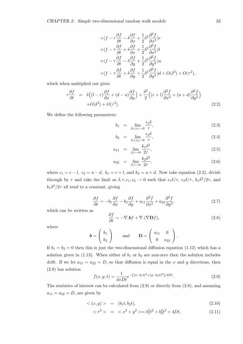
CHAPTER 2: Simple two-dimensional random walk models 33
+(f − τ∂f
∂t− δ
∂f
∂x+
1
2δ2∂2f
∂x2)r
+(f − τ∂f
∂t+ δ
∂f
∂x+
1
2δ2∂2f
∂x2)l
+(f − τ∂f
∂t− δ
∂f
∂y+
1
2δ2∂2f
∂y2)u
+(f − τ∂f
∂t+ δ
∂f
∂y+
1
2δ2∂2f
∂y2)d+O(δ3) +O(τ2),
which when multiplied out gives
τ∂f
∂t= δ
(
(l − r)∂f
∂x+ (d− u)
∂f
∂y
)
+δ2
2
(
(r + l)∂2f
∂x2+ (u+ d)
∂2f
∂y2
)
+O(δ3) +O(τ2). (2.2)
We define the following parameters:
b1 = limδ,τ,ǫ1→0
ǫ1δ
τ, (2.3)
b2 = limδ,τ,ǫ2→0
ǫ2δ
τ, (2.4)
a11 = limδ,τ→0
k1δ2
2τ, (2.5)
a22 = limδ,τ→0
k2δ2
2τ, (2.6)
where ǫ1 = r − l, ǫ2 = u− d, k1 = r+ l, and k2 = u+ d. Now take equation (2.2), divide
through by τ and take the limit as δ, τ, ǫ1, ǫ2 → 0 such that ǫ1δ/τ , ǫ2δ/τ , k1δ2/2τ , and
k1δ2/2τ all tend to a constant, giving
∂f
∂t= −b1
∂f
∂x− b2
∂f
∂y+ a11
∂2f
∂x2+ a22
∂2f
∂y2, (2.7)
which can be written as∂f
∂t= −∇.bf + ∇.(∇Df), (2.8)
where
b =
b1
b2
and D =
a11 0
0 a22
.
If b1 = b2 = 0 then this is just the two-dimensional diffusion equation (1.12) which has a
solution given in (1.13). When either of b1 or b2 are non-zero then the solution includes
drift. If we let a11 = a22 = D, so that diffusion is equal in the x and y directions, then
(2.8) has solution
f(x, y, t) =1
4πDte−((x−b1t)2+(y−b2t)2)/4Dt. (2.9)
The statistics of interest can be calculated from (2.9) or directly from (2.8), and assuming
a11 = a22 = D, are given by
< (x, y) > = (b1t, b2t), (2.10)
< r2 > = < x2 + y2 >= b21t2 + b22t
2 + 4Dt, (2.11)

CHAPTER 2: Simple two-dimensional random walk models 34
and
σ2 =< r2 > − < (x, y) >2= 4Dt. (2.12)
These solutions are comparable to the one-dimensional solutions in (1.23) and (1.25).
2.3.2 Turning probabilities dependent on position
As before, we restrict the population to moving on a two-dimensional infinite lattice. At
each time step τ an individual can move a distance δ either up, down, left or right with
probabilities dependent on position, given by u(x, y), d(x, y), l(x, y) and r(x, y) respec-
tively, where u(x, y) + d(x, y) + l(x, y) + r(x, y) ≤ 1, or remain at the same position with
probability 1 − u(x, y) − l(x, y) − d(x, y) − r(x, y).
If we take a forward time step, then the number density of individuals at position (x, y)
is given by
f(x, y, t) = f(x, y, t− τ)[1 − l(x, y) − r(x, y) − u(x, y) − d(x, y)]
+f(x− δ, y, t − τ)r(x− δ, y) + f(x+ δ, y, t − τ)l(x+ δ, y)
+f(x, y − δ, t− τ)u(x, y − δ) + f(x, y + δ, t− τ)d(x, y + δ).
We can expand each term as a Taylor series up to O(δ2) and O(τ), giving
f(x, y, t) = (f − τ∂f
∂t)[1 − l − r − u− d]
+(f − τ∂f
∂t− δ
∂f
∂x+δ2
2
∂2f
∂x2)(r − δ
∂r
∂x+δ2
2
∂2r
∂x2)
+(f − τ∂f
∂t+ δ
∂f
∂x+δ2
2
∂2f
∂x2)(l + δ
∂l
∂x+δ2
2
∂2l
∂x2)
+(f − τ∂f
∂t− δ
∂f
∂y+δ2
2
∂2f
∂y2)(u− δ
∂u
∂y+δ2
2
∂2u
∂y2)
+(f − τ∂f
∂t+ δ
∂f
∂y+δ2
2
∂2f
∂y2)(d + δ
∂d
∂y+δ2
2
∂2d
∂y2)
+O(δ3) +O(τ2) +O(δτ),
which when multiplied out gives
τ∂f
∂t= δ(
∂l
∂x− ∂r
∂x)f + δ(
∂d
∂y− ∂u
∂y)f +
δ2
2(∂2r
∂x2+∂2l
∂x2)f
+δ2
2(∂2d
∂y2+∂2u
∂y2)f + δ(l − r)
∂f
∂x+ δ(d− u)
∂f
∂y
+δ2(∂l
∂x+∂r
∂x)∂f
∂x+ δ2(
∂d
∂y+∂u
∂y)∂f
∂y+δ2
2(l + r)
∂2f
∂x2
+δ2
2(d+ u)
∂2f
∂y2+O(δ3) +O(τ2) +O(δτ). (2.13)
We define the following parameters:
b1 = limδ,τ,ǫ1→0
ǫ1δ
τ, (2.14)

CHAPTER 2: Simple two-dimensional random walk models 35
b2 = limδ,τ,ǫ2→0
ǫ2δ
τ, (2.15)
a11 = limδ,τ→0
k1δ2
2τ, (2.16)
a22 = limδ,τ→0
k2δ2
2τ, (2.17)
where ǫ1 = r − l, ǫ2 = u− d, k1 = r + l and k2 = u+ d. Similarly, we have
∂b1∂x
= limδ,τ,ǫ1→0
∂ǫ1∂x
δ
τ,
∂2b1∂x2
= limδ,τ,ǫ1→0
∂2ǫ1∂x2
δ
τetc.
We now take equation (2.13), divide through by τ and take the limit as δ, τ, ǫ1, ǫ2 → 0
such that ǫ1δ/τ , ǫ2δ/τ , k1δ2/2τ , and k1δ
2/2τ all tend to a constant, giving
∂f
∂t= −∂(fb1)
∂x− ∂(fb2)
∂y+∂2(fa11)
∂x2+∂2(fa22)
∂y2, (2.18)
which can be written as∂f
∂t= −∇.(bf) + ∇.(∇(Df)), (2.19)
where
b =
b1(x, y)
b2(x, y)
and D =
a11(x, y) 0
0 a22(x, y)
.
This is the same result as the previous case (2.8), except that b and D are now dependent
on position. This is a special case of the Fokker–Planck diffusion equation.
In principle equation (2.19) can be solved if the dependence of the parameters in D and
b on (x, y) are known but this can be extremely complex so we do not try and solve for
general solutions here.
2.4 Multi-directional discrete direction model and continu-
ous direction model
2.4.1 Multi-directional discrete direction model
Suppose we now allow the population to move around freely in any direction and not
restrict ourselves to a lattice. Suppose at each time step τ an individual can move a
distance δ in one of N possible directions given by θi, where θi ∈ θ1, ..., θN : 0 ≤ θi < 2π,with probability dependent on position given by pi(x, y), where
N∑
i=1
pi(x, y) ≤ 1.

CHAPTER 2: Simple two-dimensional random walk models 36
θ
θ θ
i
j k
t0
t1 t2
θ = 0
Figure 2.2: Example of a multi-directional random walk.
If we take a forward time step then the number density, f(x, y), of individuals at position
(x, y) is given by
f(x, y, t) =N∑
i=1
(
f(x− δ sin θi, y − δ cos θi, t− τ)pi(x− δ sin θi, y − δ cos θi))
+f(x, y, t− τ)(
1 −N∑
i=1
pi(x, y))
. (2.20)
We can expand each term in the above as a Taylor series up to O(δ2) and O(τ), which
gives
f = (f − τ∂f
∂t)(
1 −N∑
i=1
pi)
+N∑
i=1
(
(f − τ∂f
∂t− δ sin θi
∂f
∂x− δ cos θi
∂f
∂y
+δ2 sin θi cos θi∂2f
∂x∂y+δ2 sin2 θi
2
∂2f
∂x2+δ2 cos2 θi
2
∂2f
∂y2)
(pi − δ sin θi∂pi∂x
− δ cos θi∂pi∂y
+ δ2 cos θi sin θi∂2pi∂x∂y
+δ2 sin 2θi
2
∂2pi∂x2
+δ2 cos2 θi
2
∂2pi∂y2
))
+O(δ3) +O(τ2) +O(δτ). (2.21)
We can expand this out to give
τ∂f
∂t= δ
(
−N∑
i=1
(sin θi∂pi∂x
) −N∑
i=1
(cos θi∂pi∂y
))
f
+δ2
2
(
N∑
i=1
(2 cos θi sin θi∂2pi∂x∂y
) +N∑
i=1
(sin2 θi∂2pi∂x2
) +N∑
i=1
(cos2 θi∂2pi∂y2
))
f
+ δ(
−N∑
i=1
(sin θipi))∂f
∂x+ δ2
(
N∑
i=1
(sin2 θi∂pi∂x
) +N∑
i=1
(sin θi cos θi∂pi∂y
))∂f
∂x
+ δ(
−N∑
i=1
(cos θipi))∂f
∂y+ δ2
(
N∑
i=1
(cos2 θi∂pi∂y
) +N∑
i=1
(sin θi cos θi∂pi∂x
))∂f
∂y
+ δ2(
N∑
i=1
(sin θi cos θipi)) ∂2f
∂x∂y+δ2
2
(
N∑
i=1
(sin2 θipi))∂2f
∂x2

CHAPTER 2: Simple two-dimensional random walk models 37
+δ2
2
(
N∑
i=1
(cos2 θipi))∂2f
∂y2+O(δ3) +O(τ2) +O(δτ). (2.22)
We define the following parameters:
b1 = limδ,τ,ǫ1→0
(
ǫ1δ
τ
)
, (2.23)
b2 = limδ,τ,ǫ2→0
(
ǫ2δ
τ
)
, (2.24)
a11 = limδ,τ→0
(
N∑
i=1
(pi sin2 θi)
δ2
2τ
)
, (2.25)
a22 = limδ,τ→0
(
N∑
i=1
(pi cos2 θi)
δ2
2τ
)
, (2.26)
a12 = limδ,τ→0
(
N∑
i=1
(pi sin θi cos θi)δ2
2τ
)
, (2.27)
where ǫ1 =∑Ni=1(pi sin θi), ǫ2 =
∑Ni=1(pi cos θi). In a similar way we have
∂b1∂x
= limδ,τ,ǫ1→0
(
∂ǫ1∂x
δ
τ
)
,
∂2b1∂x2
= limδ,τ,ǫ1→0
(
∂2ǫ1∂x2
δ
τ
)
etc.
We now take equation (2.22), divide through by τ and take the limit as δ, τ, ǫ1, ǫ2 → 0
such that ǫ1δ/τ , ǫ2δ/τ , and δ2/τ all tend to a constant.
After rearranging, we get
∂f
∂t= −∂(fb1)
∂x− ∂(fb2)
∂y+ 2
∂2(fa12)
∂x∂y+∂2(fa11)
∂x2+∂2(fa22)
∂y2(2.28)
which can be written as∂f
∂t= −∇.(bf) + ∇.(∇(Df)) (2.29)
where
b =
b1
b2
and D =
a11 a12
a12 a22
.
This is the same equation as (2.19), except that the diffusion matrix D now has non-zero
off-diagonal terms. These off-diagonal terms arise from the covariance we introduced by
allowing movement in both the x and y directions during one step.
2.4.2 Continuous direction model
We can extend the above result to allow movement in any direction rather than just one
of N directions. Suppose at each time step τ an individual can either move a distance δ
in any direction θ, where −π ≤ θ < π, with probability dependent on position given by
p(θ;x, y), where∫ π
−πp(θ;x, y) dθ ≤ 1,

CHAPTER 2: Simple two-dimensional random walk models 38
or remain in the same position with probability
1 −∫ π
−πp(θ;x, y) dθ.
If we take a forward time step then the number density, f(x, y), of individuals at position
(x, y) is given by
f(x, y, t) =
∫ π
−πf(x− δ sin θ, y − δ cos θ, t− τ)p(θ;x− δ sin θ, y − δ cos θ) dθ
+f(x, y, t− τ)(
1 −∫ π
−πp(θ;x, y)dθ
)
. (2.30)
We can expand each term in the above as a Taylor series up to O(δ2) and O(τ), which
gives
f =
∫ π
−π
(
(f − τ∂f
∂t− δ sin θ
∂f
∂x− δ cos θ
∂f
∂y+ δ2 sin θ cos θ
∂2f
∂x∂y
+δ2 sin2 θ
2
∂2f
∂x2+δ2 cos2 θ
2
∂2f
∂y2)(p − δ sin θ
∂p
∂x− δ cos θ
∂p
∂y
+δ2 cos θ sin θ∂2p
∂x∂y+δ2 sin 2θ
2
∂2p
∂x2+δ2 cos2 θ
2
∂2p
∂y2))
dθ
+(f − τ∂f
∂t)(
1 −∫ π
−πp dθ
)
+O(δ3) +O(τ2) +O(δτ). (2.31)
Multiplying out gives
τ∂f
∂t= δ
(
−∫ π
−π(sin θ
∂p
∂x)dθ −
∫ π
−π(cos θ
∂p
∂y)dθ)
f
+δ2
2
(
∫ π
−π(2 cos θ sin θ
∂2p
∂x∂y)dθ +
∫ π
−π(sin2 θ
∂2p
∂x2)dθ +
∫ π
−π(cos2 θ
∂2p
∂y2)dθ)
f
+δ(
−∫ π
−π(sin θp)dθ
)∂f
∂x+ δ2
(
∫ π
−π(sin2 θ
∂p
∂x)dθ +
∫ π
−π(sin θ cos θ
∂p
∂y)dθ)∂f
∂x
+δ(
−∫ π
−π(cos θp)dθ
)∂f
∂y+ δ2
(
∫ π
−π(cos2 θ
∂p
∂y)dθ +
∫ π
−π(sin θ cos θ
∂p
∂x)dθ)∂f
∂y
+δ2(
∫ π
−π(sin θ cos θp)dθ
) ∂2f
∂x∂y+δ2
2
(
∫ π
−π(sin2 θp)dθ
)∂2f
∂x2
+δ2
2
(
∫ π
−π(cos2 θp)dθ
)∂2f
∂y2+O(δ3) +O(τ2) +O(δτ). (2.32)
We define the following parameters:
b1 = limδ,τ,ǫ1→0
(
ǫ1δ
τ
)
, (2.33)
b2 = limδ,τ,ǫ2→0
(
ǫ2δ
τ
)
, (2.34)
a11 = limδ,τ→0
(
∫ π
−π(p sin2 θ)dθ
δ2
2τ
)
, (2.35)
a22 = limδ,τ→0
(
∫ π
−π(p cos2 θ)dθ
δ2
2τ
)
, (2.36)
a12 = limδ,τ→0
(
∫ π
−π(p sin θ cos θ)dθ
δ2
2τ
)
, (2.37)

CHAPTER 2: Simple two-dimensional random walk models 39
where ǫ1 =∫ π−π(p sin θ)dθ and ǫ2 =
∫ π−π(p cos θ)dθ. In a similar way we have
∂b1∂x
= limδ,τ,ǫ1→0
(
∂ǫ1∂x
δ
τ
)
,
∂2b1∂x2
= limδ,τ,ǫ1→0
(
∂2ǫ1∂x2
δ
τ
)
etc.
We now take equation (2.32), divide through by τ and take the limit as δ, τ, ǫ1, ǫ2 → 0
such that ǫ1δ/τ , ǫ2δ/τ , and δ2/τ all tend to a constant. As with the previous models, for
the limit to be valid we must assume that the ǫ1 and ǫ2 terms and their derivatives tend to
zero in the same limit. Thus we need∫ π−π(p sin θ)dθ ∼ O(δ) and
∫ π−π(p cos θ)dθ ∼ O(δ),
which is only true if the distribution p(θ;x, y) is close to uniform when considering the
probability of moving with a particular angle θ. Thus this model will only be valid if there
is a small amount of bias and the angular distribution is close to uniform.
After rearranging, we get
∂f
∂t= −∂(fb1)
∂x− ∂(fb2)
∂y+ 2
∂2(fa12)
∂x∂y+∂2(fa11)
∂x2+∂2(fa22)
∂y2, (2.38)
which can be written as∂f
∂t= −∇.(bf) + ∇.(∇Df), (2.39)
where
b =
b1
b2
and D =
a11 a12
a12 a22
.
This is exactly the same equation that we derived for the multi-directional case (2.29). The
parameters given in (2.33)—(2.37) can be calculated if we know the form of the probability
distribution for the direction of motion, p(θ;x, y).
2.5 Solution of the Fokker–Planck diffusion equation
One can solve (2.39) after choosing an appropriate probability distribution for p(θ;x, y),
the probability of moving in a certain direction θ given the current position (x, y). Note
that p(θ;x, y) will thus be independent of the previous direction of movement — there is
no directional correlation as this is a position jump process.
2.5.1 Solution for isotropic movement
Suppose that p(θ;x, y) = 1/2π, so that there is no bias and the probability of move-
ment is independent of the (x, y) position. We would expect (2.39) to reduce to the
two-dimensional isotropic diffusion equation (1.12) with corresponding solution (1.13).
Recalling that θ = 0 in the y direction, then from (2.33)—(2.37) we have
b1 = limδ,τ,ǫ1→0
(
ǫ1δ
τ
)
= 0, (2.40)

CHAPTER 2: Simple two-dimensional random walk models 40
b2 = limδ,τ,ǫ2→0
(
ǫ2δ
τ
)
= 0, (2.41)
a11 = limδ,τ→0
(
∫ π
−π
sin2 θ
2πdθδ2
2τ
)
=δ2
4τ, (2.42)
a22 = limδ,τ→0
(
∫ π
−π
cos2 θ
2πdθδ2
2τ
)
=δ2
4τ, (2.43)
a12 = limδ,τ→0
(
∫ π
−π
sin θ cos θ
2πdθδ2
2τ
)
= 0 (2.44)
which are the same parameters as in (2.8) with r = l = u = d = 1/4, i.e. the isotropic
two-dimensional random walk. The corresponding diffusion equation is given in (1.12),
with solution in (1.13).
2.5.2 Solution for biased movement
We have discussed previously how the solution of the diffusion equation is only valid as
a long-time approximation. If we assume that this is the case, we can use the steady
state solution independent of position (so p(θ;x, y) = p(θ)) that is given by Hill & Hader’s
solutions to the Fokker–Planck equation for a circular random walk (1.100) and (1.102).
Assuming the preferred direction is given by θ0 = 0 then for sinusoidal reorientation we
have
p(θ) =1
2πI0(γ)eγ cos θ, (2.45)
where γ = 2B−1/σ20 , and for linear reorientation we have
p(θ) = B(λ)e−λθ2
, (2.46)
where λ = B−1/σ20 .
We can now calculate the parameters given in (2.33)—(2.37).
2.5.2.1 Sinusoidal model
In the following parameter equations we use p(θ) = 12πI0(γ)
eγ cos θ, where γ = 2B−1/σ20 and
I0(γ) is the modified Bessel function of the first kind and zero order. We use the standard
integral of the von Mises distribution from Mardia & Jupp (1999)
1
2πI0(κ)
∫ π
−πsinnθeκ cos θdθ = 0, (2.47)
1
2πI0(κ)
∫ π
−πcosnθeκ cos θdθ =
In(κ)
I0(κ). (2.48)
From (2.33) we have
b1 = limδ,τ,ǫ1→0
(
ǫ1δ
τ
)
= 0, (2.49)
since ǫ1 =∫ π−π(p sin θ)dθ = 0 from (2.47).

CHAPTER 2: Simple two-dimensional random walk models 41
From (2.34) we have
b2 = limδ,τ,ǫ2→0
(
ǫ2δ
τ
)
= limδ,τ,γ→0
(
I1(γ)
I0(γ)
δ
τ
)
, (2.50)
since ǫ2 =∫ π−π(p cos θ)dθ = I1(γ)/I0(γ), using (2.48).
From (2.35) we have
a11 = limδ,τ→0
(
∫ π
−π(p sin2 θ)dθ
δ2
2τ
)
(2.51)
= limδ,τ→0
(
(
1
2− I2(γ)
2I0(γ)
)
δ2
2τ
)
, (2.52)
since∫ π−π(p sin2 θ)dθ = 1/2(1 − I2(γ)/I0(γ)), using (2.48).
From (2.36) we have
a22 = limδ,τ→0
(
∫ π
−π(p cos2 θ)dθ
δ2
2τ
)
(2.53)
= limδ,τ→0
(
(
1
2+
I2(γ)
2I0(γ)
)
δ2
τ
)
, (2.54)
since∫ π−π(p cos2 θ)dθ = 1/2(1 + I2(γ)/I0(γ)), using (2.48).
From (2.37) we have
a12 = limδ,τ→0
(
∫ π
−π(p sin θ cos θ)dθ
δ2
2τ
)
= 0, (2.55)
since∫ π−π(p sin θ cos θ)dθ = 0, using (2.47).
For this analysis to be valid we need ǫ2 ∼ O(δ), and thus I1(γ)/I0(γ) ∼ O(δ). This is
true only if γ is small, which in turn means that the reorientation parameter B−1 must
be small or the variance per unit time, σ20 , must be large. In either case this implies that
there cannot be a large amount of bias in the system and the angular distribution p(θ)
must be close to the uniform distribution.
2.5.2.2 Linear model
In the following parameter equations we use p(θ) = B(λ)e−λθ2
, where λ = d0/σ20 and B(λ)
is the normalization function defined in (1.103).
From (2.33) we have
b1 = limδ,τ,ǫ1→0
(
ǫ1δ
τ
)
= 0, (2.56)
since ǫ1 =∫ π−π(p sin θ)dθ = 0 as p(θ) is symmetric about θ = 0.
From (2.34) we have
b2 = limδ,τ,ǫ2→0
(
ǫ2δ
τ
)
, (2.57)

CHAPTER 2: Simple two-dimensional random walk models 42
where ǫ2 = B(λ)∫ π−π cos θe−λθ
2
dθ.
From (2.35) we have
a11 = limδ,τ→0
(
∫ π
−π(p sin2 θ)dθ
δ2
2τ
)
(2.58)
= limδ,τ→0
(
(
1 −∫ π
−πcos 2θe−λθ
2
dθ
)
δ2
4τ
)
. (2.59)
From (2.36) we have
a22 = limδ,τ→0
(
∫ π
−π(p cos2 θ)dθ
δ2
2τ
)
(2.60)
= limδ,τ→0
(
(
1 +
∫ π
−πcos 2θe−λθ
2
dθ
)
δ2
4τ
)
. (2.61)
From (2.37) we have
a12 = limδ,τ→0
(
∫ π
−π(p sin θ cos θ)dθ
δ2
2τ
)
= 0, (2.62)
since p(θ) is symmetric about θ = 0.
As in the sinusoidal model, this analysis will only be valid if ǫ2 ∼ O(δ), which consequently
means that p(θ) must be close to the uniform distribution.
2.5.2.3 Solution of the Fokker–Planck equation
For both the sinusoidal and linear models b1 = a12 = 0, and (2.39) simplifies to
∂f
∂t= −b2
∂f
∂y+ a11
∂2f
∂x2+ a22
∂2f
∂y2, (2.63)
where one can substitute for b2 from either (2.50) or (2.57) depending on which model is
being used, and similarly for the parameters a11 and a22.
By inspection, we see that the following is a solution of (2.63)
f(x, y, t) =1
4π√a11
√a22t
exp
(
− x2
4a11t− (y − b2t)
2
4a22t
)
, (2.64)
where the parameters b2, a11 and a22 are dependent on the reorientation model chosen.
Solution plots for (2.64) are shown in Figure 2.3 (note that the parameter values are chosen
to illustrate the behaviour of the solution and are not necessarily ‘realistic’).
The moments < (x, y) >, < r2 >=< x2 + y2 > and σ2 can be calculated directly from
the differential equation (2.63) or from the solution (2.64), assuming that f(x, y, t) and its
derivatives tend to zero as |x|, |y| → ∞. Using either method, we have
< (x, y)(t) >= (0, b2t), (2.65)
< r2(t) >=< x2(t) + y2(t) >= b22t2 + 2(a11 + a22)t, (2.66)

CHAPTER 2: Simple two-dimensional random walk models 43
–100
–50
0
50
100
x
–50
0
50
100
150
y
0
0.0005
0.001
0.0015
0.002
0.0025
f(x,y,t)
(a) b2 = 1, a11 = 1, a22 = 10.
–100
–50
0
50
100
x
–50
0
50
100
150
y
0
0.0005
0.001
0.0015
0.002
0.0025
f(x,y,t)
(b) b2 = 10, a11 = 10, a22 = 1.
Figure 2.3: Plots showing f(x, y, t) for various parameter values at t = 10.
and
σ2(t) = 2(a11 + a22)t. (2.67)
In the simple random walk models presented previously, the walkers can have a bias in
their movement which is either fixed or dependent on the spatial position, but not de-
pendent on the previous direction of movement, i.e. there is no correlation. As suggested
in the introduction chapter, the diffusion equation and corresponding solutions can be
considered as the long-time limiting solution of the underlying process that includes cor-
relation effects. The main problem with all the diffusion-type equations we have derived
is that the solutions allow for effectively infinite propagation speeds. This comes about
because of the way we take certain limits, see for example Okubo (1980). We assume that
limδ,τ→0
δ2
τ= constant.
One can easily see that as a consequence of this we have
limδ,τ→0
δ
τ→ ∞.
Over large time scales the solution reaches a steady state and this effectively infinite
propagation can be ignored but over small timescales it is not valid. If we introduce
correlation into the model we can avoid this problem of infinite propagation and make the
model more biologically realistic.
Henderson et al. (1984) modelled the growth of the roots of the Sitka spruce as a two-
dimensional correlated but unbiased random walk on a square lattice. In their model the
probability of moving forward f, back b, left l and right r at each step was fixed (where
the directions are relative to the previous direction of movement). They derived equations

CHAPTER 2: Simple two-dimensional random walk models 44
for the mean position (which was found to be zero) and the variance in position (spread
from the origin). The variance was found to be dependent on the differences between the
probabilities of moving forward and back, (f − b), and left or right, (r − l). The variance
was found to be minimum when (f − b) was large and negative, decreasing as (r − l)
increased, and a maximum when (f − b) was large and positive. As might be expected,
the larger spread in spatial position was found to be for the motion that was most like a
straight line (corresponding to f ≈ 1).
By taking appropriate limits such that δt = δx2/σ2 for some fixed constant σ, they showed
that the limiting equation for the motion was the two-dimensional diffusion equation
(1.12). Thus even though they included correlation in the model, the limits chosen to
close the system results in a diffusion solution with the inherent ‘infinite propagation’
problem.
By modelling the random walk as the limit of a telegraph process that includes correlation
and a fixed velocity we showed that, in one dimension we can avoid the problem of infinite
propagation (see Section 1.1.4). We now attempt a similar derivation in two dimensions.
2.6 The telegraph equation in higher dimensions
The solution to the two-dimensional diffusion process with or without drift has been shown
to be only valid as a long-time approximation to the true underlying solution that includes
correlation effects. One can introduce correlation by completing a similar derivation as in
Section 1.1.4 but working with an infinite two-dimensional lattice rather than a line.
We now have four possible directions of movement — right, left, up and down. To start
with, we assume that the probability of turning is independent of the direction of movement
(so we have no bias). As before we assume a constant speed v. We split the population
into up-moving individuals α1, right-moving individuals α2, down-moving individuals α3
and left moving individuals α4, where α1 +α2 +α3 +α4 = p, the total population. At each
time step τ an individual can either move a distance δ in the direction it was previously
moving (with probability f = 1− (λ1 +λ2 +λ3)τ); or turn 90 to the left (so right-moving
becomes up-moving etc) and move a distance δ in this new direction (with probability
l = λ1τ); or turn 90 to the right (so right-moving becomes down-moving etc) and move
a distance δ in this new direction (with probability r = λ2τ); or turn 180 around (so
right-moving becomes left-moving etc) and move a distance δ in this new direction (with
probability b = λ3τ).
If we take a forward time step then the number of individuals at position x moving up,
right, down and left respectively is given by
α1(x, y, t+ τ) = fα1(x, y − δ, t) + lα2(x, y − δ, t) + bα3(x, y − δ, t) + rα4(x, y − δ, t),
α2(x, y, t+ τ) = fα2(x− δ, y, t) + lα3(x− δ, y, t) + bα4(x− δ, y, t) + rα1(x− δ, y, t),

CHAPTER 2: Simple two-dimensional random walk models 45
α3(x, y, t+ τ) = fα3(x, y + δ, t) + lα4(x, y + δ, t) + bα1(x, y + δ, t) + rα2(x, y + δ, t),
α4(x, y, t+ τ) = fα4(x+ δ, y, t) + lα1(x+ δ, y, t) + bα2(x+ δ, y, t) + rα3(x+ δ, y, t).
We can expand the above equations as Taylor series to give
α1 + τ∂α1
∂t+O(τ2) = f(α1 − δ
∂α1
∂y) + l(α2 − δ
∂α2
∂y) + b(α3 − δ
∂α3
∂y) + r(α4 − δ
∂α4
∂y)
+O(δ2),
α2 + τ∂α2
∂t+O(τ2) = f(α2 − δ
∂α2
∂x) + l(α3 − δ
∂α3
∂x) + b(α4 − δ
∂α4
∂x) + r(α1 − δ
∂α1
∂x)
+O(δ2),
α3 + τ∂α3
∂t+O(τ2) = f(α3 − δ
∂α3
∂y) + l(α4 − δ
∂α4
∂y) + b(α1 − δ
∂α1
∂y) + r(α2 − δ
∂α2
∂y)
+O(δ2),
α4 + τ∂α4
∂t+O(τ2) = f(α4 − δ
∂α4
∂x) + l(α1 − δ
∂α1
∂x) + b(α2 − δ
∂α2
∂x) + r(α3 − δ
∂α3
∂x)
+O(δ2).
We can now substitute for f, l, b and r. After dividing through by τ and taking the limit
as τ → 0 and δ → 0 such that δτ → v we get
∂α1
∂t= −v∂α1
∂y− (λ1 + λ2 + λ3)α1 + λ1α2 + λ3α3 + λ2α4, (2.68)
∂α2
∂t= −v∂α2
∂x− (λ1 + λ2 + λ3)α2 + λ1α3 + λ3α4 + λ2α1, (2.69)
∂α3
∂t= v
∂α3
∂y− (λ1 + λ2 + λ3)α3 + λ1α4 + λ3α1 + λ2α2, (2.70)
∂α4
∂t= v
∂α4
∂x− (λ1 + λ2 + λ3)α4 + λ1α1 + λ3α2 + λ2α3. (2.71)
Adding (2.68) + (2.69) + (2.70) + (2.71) gives
∂p
∂t= v
(∂(α4 − α2)
∂x+∂(α3 − α1)
∂y
)
, (2.72)
which can be differentiated to give
∂2p
∂t2= v
(∂2(α4 − α2)
∂x∂t+∂2(α3 − α1)
∂y∂t
)
. (2.73)
One can differentiate (2.69) and (2.71) with respect to x, which after rearranging gives
∂(α4 − α2)
∂x∂t= v
∂2(α2 + α4)
∂x2− (λ1 + λ2 + 2λ3)
(α4 − α2)
∂x+ (λ2 − λ1)
∂(α3 − α1)
∂x. (2.74)
Similarly, after differentiating (2.68) and (2.70) with respect to y and rearranging we get
∂(α3 − α1)
∂y∂t= v
∂2(α1 + α3)
∂y2− (λ1 + λ2 + 2λ3)
(α3 − α1)
∂y+ (λ2 − λ1)
∂(α2 − α4)
∂y. (2.75)
We can substitute (2.74) and (2.75) back into (2.73) and use (2.72) to give
∂2p
∂t2= v2
(∂2(α2 + α4)
∂x2+∂2(α1 + α3)
∂y2
)
− v(λ1 + λ2 + 2λ3)∂p
∂t
+(λ2 − λ1)(∂(α3 − α1)
∂x− ∂(α4 − α2)
∂y
)
. (2.76)

CHAPTER 2: Simple two-dimensional random walk models 46
One can see that the two-dimensional equation we have derived has a very similar form to
our original one-dimensional telegraph equation (1.41), but the system cannot be written
in terms of the total population p. We could solve equations (2.68)—(2.71) simultaneously
to find solutions for α1-α4 but we cannot solve directly to find a solution for p.
It is possible to do a similar analysis for models with more than four directions. However,
as above, this results in a system of equations that cannot be closed to find an equation
for p, see also the discussions in Othmer & Hillen (2000; 2002).
The two-dimensional telegraph equation does exist and is straightforward to solve in princi-
ple, see Morse & Feshbach (1953). However it is not the limiting equation to the correlated
random walk process we have described above.
2.7 Conclusions
In this chapter we have shown how it is straightforward to extend the one-dimensional
uncorrelated random walk process (a position jump process) to a two-dimensional lattice
and derive the Fokker–Planck diffusion equation. It is possible to make the probabilities
of moving in a certain direction dependent on position, extend the allowed moves from a
lattice to a discrete number of movement directions with differing probabilities, or allow a
continuous range of directions of movement on the unit circle with probability distribution
p(θ), all of which result in similar Fokker–Planck equations, albeit with slightly different
parameter definitions. We can use the experimental results of Hill & Hader and substitute
p(θ) for their predicted long-time angular distribution and calculate the parameters in the
Fokker–Planck equation, but this is only valid if we have a small amount of bias in the sys-
tem and p(θ) is close to uniform. All the solutions of the Fokker–Planck equation allow for
effectively infinite propagation and thus can only be considered large time approximations
to the true solutions.
If we try and extend the one-dimensional telegraph process (a velocity jump process) to
two dimensions with a simple correlated random walk on a lattice we cannot derive a
closed equation for the probability distribution.
To find out information about the underlying spatial distribution we need to approach the
problem in a slightly different manner. In Chapters 3, 4 and 5 we discuss a method of
calculating the moments of the spatial distribution rather then trying to find an equation
that describes the spatial distribution directly.
The main results of this chapter are summarised below:
• It is straightforward to develop the one-dimensional uncorrelated random walk model
to a two-dimensional lattice and using difference equations, the two-dimensional
Fokker–Planck diffusion equation can be derived.

CHAPTER 2: Simple two-dimensional random walk models 47
• Bias is introduced by setting the probability of moving in a particular direction to be
greater than the probability of moving in any other direction. The Fokker–Planck
equation will then include drift terms.
• The probabilities of moving in a certain direction can be made dependent on position,
which results in a similar Fokker–Planck equation that has parameters that are
spatially dependent.
• The model can easily be extended from a lattice to a continuous angle probability
distribution p(θ) which results in the same Fokker–Planck diffusion equation.
• The long-time angular distribution for sinusoidal or linear reorientation from Hill &
Hader can be substituted for p(θ) and the parameters in the Fokker–Planck equation
calculated. However, this is only valid if there is a small amount of bias and p(θ) is
close to uniform.
• All the solutions of the Fokker–Planck diffusion equation allow for effectively infinite
propagation and thus can only be considered as long-time approximations to the
true solutions.
• It is not possible to extend the one-dimensional correlated random walk telegraph
process to two dimensions to derive a closed equation for the population distribution.
Chapter 3
Spatial statistics of
two-dimensional velocity jump
processes
3.1 Introduction
We have seen in the previous chapter (Section 2.6) that it is not possible to derive the
telegraph equation in two dimensions for our simple random walk model. A different
method must be used to get information about the system. Although it does not seem
possible to find a simple equation that describes the spatial distribution for all time, it
is possible to calculate the moments of this distribution. Equations (1.22) and (1.24) are
simple to solve and were easy to derive from the differential equation that describes the
underlying spatial distribution.
When looking at models of dispersal in biological systems, Othmer et al. (1988) suggested
a generalized equation to model velocity jump processes and derived a ‘linear transport
equation’ for the underlying spatial and velocity distribution p(x,v, t). Although they
did not try to solve directly for p(x,v, t), they showed how to derive equations for the
moments of the distribution from the linear transport equation.
In this chapter we present the velocity jump process model of Othmer et al. (1988) and
explain all their working and methods (that were unpublished in their paper). We shall
then extend this velocity jump process model and method of taking moments in later
chapters.
48

CHAPTER 3: Spatial statistics of two-dimensional velocity jump processes 49
3.2 Generalized equation for velocity jump processes
3.2.1 Generalized model
Let p(x,v, t) be the density function for individuals in a 2n-dimensional phase space with
coordinates (x,v), where x ∈ Rn is the position of an individual, and v ∈ Rn is its
velocity. Then p(x,v, t)dxdv is the number density of individuals with position between
x and x + dx and velocity between v and v + dv, and
n(x, t) =
∫
p(x,v, t)dv (3.1)
is the number density of individuals at x, whatever their velocity. As p(x,v, t) is a density
function we have p(x,v, t) ≥ 0 ∀ x,v, t. We assume that p(x,v, t) is integrable, and that
p(x,v, t) → 0 as |x| → ∞. The evolution of p is governed by the partial differential
equation∂p
∂t+ ∇
x.vp+ ∇
v.Fp = R, (3.2)
where F denotes the external force acting on the individuals and R is the rate of change of
p due to reaction, random choice of velocity, etc. We assume that F ≡ 0 and that the only
process that contributes to the changes on the right hand side of (3.2) is a process that
generates random velocity changes. We assume that the random velocity changes are the
result of a Poisson process of intensity λ, where λ may depend upon other variables (see
for example Grimmett & Stirzaker (2001)). Thus λ−1 is a mean time between the random
choices of direction. The net rate at which individuals enter the phase-space volume at
(x,v) is given by(
∂p
∂t
)
sp= −λp+ λ
∫
T (v,v′)p(x,v′, t)dv′ (3.3)
where ‘sp’ denotes the change due to the stochastic process. The kernel T (v,v′) is the
probability of a change in velocity from v′ to v , given that a reorientation occurs, and
therefore T (v,v′) is non-negative and normalised so that
∫
T (v,v′)dv = 1. (3.4)
This normalization condition just means that no individuals are lost during the process
of changing velocity. We assume that T (v,v′) is independent of the time between jumps.
Applying the above assumptions means that (3.2) becomes
∂p
∂t+ ∇
x.vp = −λp+ λ
∫
T (v,v′)p(x,v′, t)dv′. (3.5)
Equation (3.5) is the linear transport equation first introduced to model the velocity jump
process by Othmer et al. (1988), and also discussed more recently by Othmer & Hillen
(2000; 2002).
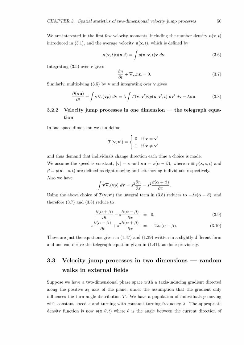
CHAPTER 3: Spatial statistics of two-dimensional velocity jump processes 50
We are interested in the first few velocity moments, including the number density n(x, t)
introduced in (3.1), and the average velocity u(x, t), which is defined by
n(x, t)u(x, t) =
∫
p(x,v, t)v dv. (3.6)
Integrating (3.5) over v gives∂n
∂t+ ∇
x.nu = 0. (3.7)
Similarly, multiplying (3.5) by v and integrating over v gives
∂(nu)
∂t+
∫
v∇.(vp) dv = λ
∫
T (v,v′)vp(x,v′, t) dv′ dv− λnu. (3.8)
3.2.2 Velocity jump processes in one dimension — the telegraph equa-
tion
In one space dimension we can define
T (v,v′) =
0 if v = v′
1 if v 6= v′
and thus demand that individuals change direction each time a choice is made.
We assume the speed is constant, |v| = s and nu = s(α − β), where α ≡ p(x, s, t) and
β ≡ p(x,−s, t) are defined as right-moving and left-moving individuals respectively.
Also we have∫
v∇.(vp) dv = s2∂n
∂x= s2
∂(α+ β)
∂x.
Using the above choice of T (v,v′) the integral term in (3.8) reduces to −λs(α− β), and
therefore (3.7) and (3.8) reduce to
∂(α + β)
∂t+ s
∂(α− β)
∂x= 0, (3.9)
s∂(α− β)
∂t+ s2
∂(α+ β)
∂x= −2λs(α− β). (3.10)
These are just the equations given in (1.37) and (1.39) written in a slightly different form
and one can derive the telegraph equation given in (1.41), as done previously.
3.3 Velocity jump processes in two dimensions — random
walks in external fields
Suppose we have a two-dimensional phase space with a taxis-inducing gradient directed
along the positive x1 axis of the plane, under the assumption that the gradient only
influences the turn angle distribution T . We have a population of individuals p moving
with constant speed s and turning with constant turning frequency λ. The appropriate
density function is now p(x, θ, t) where θ is the angle between the current direction of

CHAPTER 3: Spatial statistics of two-dimensional velocity jump processes 51
motion and the positive x1-axis. Thus the direction of travel is ξ = (cos θ, sin θ) and the
direction of the gradient is ξ1 = (1, 0). The evolution equation (3.5) reduces to
∂p
∂t+ sξ.∇
xp = −λp+ λ
∫ π
−πT (θ, θ′) p(x, θ′, t) dθ′. (3.11)
When modelling the motion of leukocytes in a constant chemotactic gradient, Othmer et
al. assumed that the turning angle distribution T is the sum of a symmetric probability
distribution h(δ), where δ = θ − θ′, and a bias term k(θ) that results from the taxis-
inducing gradient. Since the gradient is directed along the x1-axis, the bias term takes its
maximum at θ = 0, and is symmetric about θ = 0, see Figure 3.1. Thus
T (θ, θ′) = h(θ − θ′) + k(θ), (3.12)
where T ≥ 0 for all (θ, θ′) and h and k are normalized as follows:
∫ π
−πh(δ) dδ = 1,
∫ π
−πk(θ) dθ = 0,
∫ π
−πT (θ, θ′) dθ = 1, (3.13)
and also
∫ π
−πh(δ) cos δ dδ = ψd is defined as the directional persistence, (3.14)
and
∫ π
−πk(θ) cos θ dθ = χ is defined as the taxis coefficient. (3.15)
π−π
h
−π π
k
θ
(θ)
δ
(δ)
Figure 3.1: Sketch of the probability distributions for h(δ) and k(θ) as used by Othmer et
al. (1988).
3.3.1 Defining statistics of interest
Othmer et al. used (3.12) to calculate the statistics of interest, which include the mean
location of cells H(t), their mean squared displacement D2(t), and their mean velocity
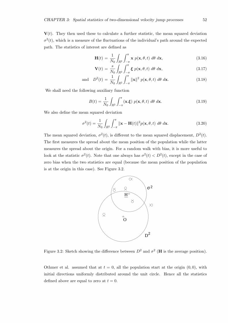
CHAPTER 3: Spatial statistics of two-dimensional velocity jump processes 52
V(t). They then used these to calculate a further statistic, the mean squared deviation
σ2(t), which is a measure of the fluctuations of the individual’s path around the expected
path. The statistics of interest are defined as
H(t) =1
N0
∫
R2
∫ π
−πx p(x, θ, t) dθ dx, (3.16)
V(t) =s
N0
∫
R2
∫ π
−πξ p(x, θ, t) dθ dx, (3.17)
and D2(t) =1
N0
∫
R2
∫ π
−π‖x‖2 p(x, θ, t) dθ dx. (3.18)
We shall need the following auxiliary function
B(t) =1
N0
∫
R2
∫ π
−π(x.ξ) p(x, θ, t) dθ dx. (3.19)
We also define the mean squared deviation
σ2(t) =1
N0
∫
R2
∫ π
−π‖x − H(t)‖2p(x, θ, t) dθ dx. (3.20)
The mean squared deviation, σ2(t), is different to the mean squared displacement, D2(t).
The first measures the spread about the mean position of the population while the latter
measures the spread about the origin. For a random walk with bias, it is more useful to
look at the statistic σ2(t). Note that one always has σ2(t) < D2(t), except in the case of
zero bias when the two statistics are equal (because the mean position of the population
is at the origin in this case). See Figure 3.2.
O
H
D2
σ 2
Figure 3.2: Sketch showing the difference between D2 and σ2 (H is the average position).
Othmer et al. assumed that at t = 0, all the population start at the origin (0, 0), with
initial directions uniformly distributed around the unit circle. Hence all the statistics
defined above are equal to zero at t = 0.

CHAPTER 3: Spatial statistics of two-dimensional velocity jump processes 53
3.3.2 Deriving equations for spatial statistics
3.3.2.1 Changing the order of integration
We use Fubini’s theorem (see for example Cox (1998)) so that the order of integration can
be changed from dθ dx to dx dθ and dθ′ dθ to dθ dθ′.
If a(θ) and b(x) are bounded over the integral range (−π to π) and R2 respectively, then
the following result holds
∫
R2
∫ π
−πa(θ)b(x) dθ dx =
∫ π
−π
∫
R2
a(θ)b(x) dx dθ, (3.21)
and if f(θ) and g(θ′) are bounded over the integral range (−π to π) then the following
holds∫ π
−π
∫ π
−πf(θ)g(θ′) dθ′ dθ =
∫ π
−π
∫ π
−πf(θ)g(θ′) dθ dθ′. (3.22)
3.3.2.2 The divergence theorem
We shall make use of the divergence theorem (see for example Cox (1998)). The divergence
theorem states that in three-dimensional space the integral of the gradient of a function
is the same as the integral around the surface of the normal to the function.
∫
V∇
x.u dV =
∫
∂Vu.n dS.
The divergence theorem can be shown to hold in two dimensions as well, and we can write
∫
R2
∇x.u dx =
∫
Su.n dS,
where S is now the boundary surrounding our domain R2. Since we have assumed an
infinite domain, S will be the boundary at |x| → ∞. Now, because we have a finite
speed of propagation and start at x = 0, we make the assumption that within finite time
p(x, θ, t) = 0 on S. Hence all functions of the form up(x, θ, t), where u is a bounded vector
function, are zero on S. Thus
∫
R3
∇x.(up) dx =
∫
S(up).n dS = 0. (3.23)
In the subsequent analysis we will need to use the following equations that are straight-
forward to derive using the properties of the gradient and divergence functions. If a is a
scalar function then
∫
R2
−a(ξ.∇xp) dx =
∫
R2
(−∇x.(ξap) + pξ.(∇
xa)) dx =
∫
R2
pξ.(∇xa) dx (3.24)
since∫
R2 −∇x.(ξap) dx = 0 from (3.23).
If v is a vector function then
∫
R2
−v(ξ.∇xp) dx =
∫
R2
(−ξ.∇x(vp) + p(ξ.∇
x)v) dx. (3.25)

CHAPTER 3: Spatial statistics of two-dimensional velocity jump processes 54
Rewriting the second term in the right hand side of the above gives
∫
R2
−v(ξ.∇xp) dx =
∫
R2
(−∇x.(ξv1p)ξ1 −∇
x.(ξv2p)ξ2 + p(ξ.∇
x)v) dx, (3.26)
where ξ1 = (1, 0) and ξ2 = (0, 1). Using (3.23), the first two terms in the right hand side
of the above are zero and we get
∫
R2
−v(ξ.∇xp) dx =
∫
R2
(p(ξ.∇x)v) dx. (3.27)
3.3.2.3 Deriving equation for H(t)
Multiply the original equation (3.11) by x, integrate over θ and x, and divide by N0, to
give
1
N0
∫
R2
∫ π
−πx∂p
∂tdθ dx = − s
N0
∫
R2
∫ π
−πx (ξ.∇
xp) dθ dx
− λ
N0
∫
R2
∫ π
−πx p dθ dx
+λ
N0
∫
R2
∫ π
−π
∫ π
−πx T (θ, θ′) p(θ′) dθ′ dθ dx.
In the final term, we can use the fact that the order of integration of dθ and dθ′ can be
changed to give the inner integral
∫ π
−πT (θ, θ′) dθ = 1.
Substituting for H(t) from (3.16) and using the divergence theorem (3.27) gives
dH
dt=
s
N0
∫
R2
∫ π
−π(pξ.∇
x)x dθ dx − λH +
λ
N0
∫
R2
∫ π
−πx p(θ′) dθ′ dx.
The last two terms now cancel, giving
dH
dt=
s
N0
∫
R2
∫ π
−πξp dθ dx.
Substituting for V(t) from (3.17) gives the final differential equation for H(t)
dH
dt= V. (3.28)
3.3.2.4 Deriving equation for V(t)
Multiply the original equation (3.11) by sξ, integrate over θ and x, and divide by N0, to
give
s
N0
∫
R2
∫ π
−πξ∂p
∂tdθ dx = − s2
N0
∫
R2
∫ π
−πξ (ξ.∇
xp) dθ dx
− sλ
N0
∫
R2
∫ π
−πξ p dθ dx
+sλ
N0
∫
R2
∫ π
−π
∫ π
−πξ T (θ, θ′) p(θ′) dθ′ dθ dx.

CHAPTER 3: Spatial statistics of two-dimensional velocity jump processes 55
The first term in the right hand side of the above is zero due to the divergence theorem
(3.27). Recalling that ξ = (cos θ, sin θ) and substituting for V(t) from (3.17) and for
T (θ, θ′) from (3.12), gives
dV
dt= −λV +
sλ
N0
∫
R2
∫ π
−π
∫ π
−π(cos θ, sin θ) (h(θ − θ′) + k(θ)) p(θ′) dθ′ dθ dx.
The order of the integral in the above can be changed (changing dθ and dθ′) to give
dV
dt= − λV +
sλ
N0
∫
R2
∫ π
−π
∫ π
−π(cos θ, sin θ) h(θ − θ′) p(θ′) dθ dθ′ dx
+sλ
N0
∫
R2
∫ π
−π
∫ π
−π(cos θ, sin θ) k(θ)) p(θ′) dθ dθ′ dx.
The distribution k(θ) is symmetric about θ = 0, so∫ π
−πsin θ k(θ) dθ = 0.
We also use the definition of χ from (3.14) to give
dV
dt= − λV
+sλ
N0
∫
R2
∫ π
−π
∫ π
−π(cos θ, sin θ) h(θ − θ′) p(θ′) dθ dθ′ dx + λχsξ1.
Fixing θ′, we can make the substitution δ = θ−θ′, and hence dδ = dθ. Using the standard
trigonometric identities gives
cos θ = cos δ cos θ′ − sin δ sin θ′, sin θ = sin δ cos θ′ + cos δ sin θ′.
Substituting these identities back into the equation and noting that we now have to change
the limits of integration, gives
dV
dt= − λV + λχsξ1
+sλξ1
N0
∫
R2
∫ π
−π
∫ π−θ′
−π−θ′(cos δ cos θ′ − sin δ sin θ′) h(δ) p(θ′) dδ dθ′ dx
+sλξ2
N0
∫
R2
∫ π
−π
∫ π−θ′
−π−θ′(sin δ cos θ′ + cos δ sin θ′) h(δ) p(θ′) dδ dθ′ dx.
Now, because the function being integrated is 2π-periodic, the limits from −π−θ′ to π−θ′
are the same as the limits from −π to π. The distribution h(δ) is also symmetric about
δ = 0 so that∫ π
−πsin δ h(δ) dδ = 0.
Recalling the definition of ψd from (3.15), we get
dV
dt= − λV + λχsξ1
+sλ
N0
∫
R2
∫ π
−π(cos θ′, sin θ′) ψd p(θ
′) dθ′ dx.
This simplifies todV
dt= −λ0V + λχsξ1 (3.29)
where
λ0 = λ(1 − ψd).

CHAPTER 3: Spatial statistics of two-dimensional velocity jump processes 56
3.3.2.5 Deriving equation for D2(t)
Multiply the original equation (3.11) by ‖x‖2, integrate over θ and x, and divide by N0,
to give
1
N0
∫
R2
∫ π
−π‖x‖2 ∂p
∂tdθ dx = − s
N0
∫
R2
∫ π
−π‖x‖2 (ξ.∇
xp) dθ dx
− λ
N0
∫
R2
∫ π
−π‖x‖2 p dθ dx
+λ
N0
∫
R2
∫ π
−π
∫ π
−π‖x‖2 T (θ, θ′) p(θ′) dθ′ dθ dx.
In the final term, we use the fact that the order of integration of dθ and dθ′ can be
changed to give the inner integral
∫ π
−πT (θ, θ′) dθ = 1.
Substituting for D2(t) from (3.18) and using the divergence theorem (3.24) gives
dD2
dt=
s
N0
∫
R2
∫ π
−π(ξp).∇
x(‖x‖2) dθ dx
− λD2 +λ
N0
∫
R2
∫ π
−π‖x‖2 p(θ′) dθ′ dx.
The final two terms cancel, giving
dD2
dt=
s
N0
∫
R2
∫ π
−π(ξp).∇
x(‖x‖2) dθ dx.
This givesdD2
dt=
s
N0
∫
R2
∫ π
−π(ξp).(2x1, 2x2) dθ dx
which can be rewritten as
dD2
dt=
2s
N0
∫
R2
∫ π
−π(ξ.x)p dθ dx.
Finally, we can substitute for B(t) from (3.19) to give the final differential equation for
D2(t),dD2
dt= 2sB. (3.30)
3.3.2.6 Deriving equation for B(t)
Multiply the original equation (3.11) by (x.ξ), integrate over θ and x, and divide by N0,
to give
1
N0
∫
R2
∫ π
−π(x.ξ)
∂p
∂tdθ dx = − s
N0
∫
R2
∫ π
−π(x.ξ)(ξ.∇
xp) dθ dx
− λ
N0
∫
R2
∫ π
−π(x.ξ) p dθ dx
+λ
N0
∫
R2
∫ π
−π
∫ π
−π(x.ξ) T (θ, θ′) p(θ′) dθ′ dθ dx.

CHAPTER 3: Spatial statistics of two-dimensional velocity jump processes 57
Substituting for B(t) from (3.19) and for T (θ, θ′) from (3.12), and using the divergence
theorem (3.24) gives
dB
dt=
s
N0
∫
R2
∫ π
−πp dθ dx− λB
+λ
N0
∫
R2
∫ π
−π
∫ π
−π(x1 cos θ + x2 sin θ) (h(θ − θ′) + k(θ)) p(θ′) dθ′ dθ dx.
The order of the integration in the above can be changed (changing dθ and dθ′) to give
dB
dt= s− λB +
λ
N0
∫
R2
∫ π
−π
∫ π
−π(x1 cos θ + x2 sin θ) k(θ) p(θ′) dθ dθ′ dx
+λ
N0
∫
R2
∫ π
−π
∫ π
−π(x1 cos θ + x2 sin θ) (θ − θ′) p(θ′) dθ dθ′ dx
The distribution k(θ) is symmetric about θ = 0 so that∫ π
−πsin θ k(θ) dθ = 0.
We use the definition of χ from (3.14) to give
dB
dt= s− λB + λχx1 +
λ
N0
∫
R2
∫ π
−π(x1 cos θ + x2 sin θ) h(θ − θ′) p(θ′) dθdθ′ dx,
where
x1 =1
N0
∫
R2
∫ π
−πx1 p(θ
′) dθ′dx = H.ξ1. (3.31)
Fixing θ′, we can make the substitution δ = θ − θ′, and hence have dδ = dθ. Using the
standard trigonometric identities we have
cos θ = cos δ cos θ′ − sin δ sin θ′, sin θ = sin δ cos θ′ + cos δ sin θ′.
Substituting back into the equation and noting that we now have to change the limits of
integration, gives
dB
dt= s− λB + λχx1
+λ
N0
∫
R2
∫ π
−π
∫ π−θ′
−π−θ′(x1 cos δ cos θ′ − x1 sin δ sin θ′) h(δ) p(θ′) dδdθ′ dx
+λ
N0
∫
R2
∫ π
−π
∫ π−θ′
−π−θ′(x2 sin δ cos θ′ + x2 cos δ sin θ′) h(δ) p(θ′) dδdθ′ dx.
Now, because the function being integrated is 2π-periodic, the limits from −π−θ′ to π−θ′
are the same as the limits from −π to π. The distribution h(δ) is symmetric about δ = 0,
so∫ π
−πsin δ h(δ) dδ = 0.
Recalling the definition of ψd from (3.15), we get
dB
dt= s− λB + λχx1 +
λ
N0
∫
R2
∫ π
−π(x1 cos θ′ + x2 sin θ′) ψd p(θ
′) dδdθ′ dx.
This simplifies todB
dt= s− λ0B + λχx1. (3.32)

CHAPTER 3: Spatial statistics of two-dimensional velocity jump processes 58
3.3.2.7 Deriving equation for σ2(t)
Rather than derive a differential equation for σ2(t), we derive an equation that relates it
to the other statistics defined earlier.
σ2(t) =1
N0
∫
R2
∫ π
−π‖x − H(t)‖2p(x, θ, t) dθdx
=1
N0
∫
R2
∫ π
−π(x − H(t)).(x − H(t))p(x, θ, t) dθdx
=1
N0
∫
R2
∫ π
−π(x.x− 2x.H(t) + H(t).H(t))p(x, θ, t) dθdx
The H(t) terms can be taken outside the integral (we are taking the average of an average),
and using the definition of D2(t), we have
σ2(t) = D2(t) − 2H(t)1
N0
∫
R2
∫ π
−πx p(x, θ, t) dθdx + H(t).H(t)
= D2(t) − 2‖H(t)‖2 + ‖H(t)‖2.
So finally we have
σ2(t) = D2(t) − ‖H(t)‖2. (3.33)
3.3.2.8 Final system of equations
The final system of equations that Othmer et al. derived is closed due to their choice of
probability distributions for the reorientation kernel T (θ, θ′). The system is
dH
dt= V, (3.34)
dV
dt= −λ0V + λχsξ1, (3.35)
dD2
dt= 2sB, (3.36)
anddB
dt= s− λ0B + λχx1, (3.37)
where
ξ1 = (1, 0) (the direction of the gradient),
x1 = H.ξ1,
and λ0 = λ(1 − ψd).
We also have the equation relating σ2 to H(t) and D2(t),
σ2(t) = D2(t) − ‖H(t)‖2. (3.38)
3.3.3 Solving equations for spatial statistics
The above system of differential equations is straightforward to solve as all the equations
are linear.

CHAPTER 3: Spatial statistics of two-dimensional velocity jump processes 59
3.3.3.1 Solution for V(t)
From (3.35) and assuming that V(0) = 0, we get
V(t) = sλχ
λ0(1 − e−λ0t)ξ1.
This can be written in the form Othmer et al. give in their paper,
V(t) = sχ
1 − ψd(1 − e−λ0t)ξ1. (3.39)
As t tends to infinity, the mean velocity of movement becomes parallel to the direction of
the gradient and approaches the value
V∞ = sχ
1 − ψdξ1.
For this to be consistent we must have (1−ψd) ≥ χ. We cannot have an absolute velocity
that is greater than the speed of movement.
3.3.3.2 Solution for H(t)
From (3.34) and assuming that H(0) = 0, we get
H(t) = sχ
1 − ψd
(
t− 1
λ0(1 − e−λ0t)
)
ξ1. (3.40)
3.3.3.3 Solution for B(t)
From (3.37) and assuming that B(0) = 0, we get
B(t) =s
λ0
(
1 − e−λ0t + C2I
(
λ0t− 2(1 − e−λ0t) + λ0te−λ0t
))
, (3.41)
where C2I = λ2χ2/λ2
0.
3.3.3.4 Solution for D2(t)
From (3.36) and assuming that D2(0) = 0, we get
D2(t) =2s2
λ0
[
(1 − 2C2I )t− C2
I te−λ0t +
(3C2I − 1)
λ0(1 − e−λ0t) +
C2Iλ0t
2
2
]
. (3.42)
3.3.3.5 Solution for σ2(t)
Substituting (3.40) and (3.42) into (3.33) gives
σ2(t) =2s2
λ0
[
(1 − 2C2I )t− C2
I te−λ0t +
(3C2I − 1)
λ0(1 − e−λ0t) +
C2Iλ0t
2
2
]
−2s2
λ0
[ C2I
2λ0(λ2
0t2 + e−2λ0t + 1 + 2λ0te
−λ0t − 2λ0t− 2e−λ0t)]
.

CHAPTER 3: Spatial statistics of two-dimensional velocity jump processes 60
This simplifies to
σ2(t) =2s2
λ0
(
(1 − C2I )t− 2C2
I te−λ0t +
(2C2I − 1)
λ0(1 − e−λ0t) +
C2I
2λ0(1 − e−2λ0t)
)
. (3.43)
Note that in the paper of Othmer et al. there is an error in their solution for σ2(t). They
incorrectly have (1 − e−λ0t)2 instead of (1 − e−2λ0t) in the final term in the equation.
As t tends to infinity the solution tends to
σ2(t) ∼ 2s2
λ0
[
(1 − C2I )t+
1
λ0(5
2C2I − 1)
]
. (3.44)
The quantity
CI =χ
1 − ψd
measures the net effect of the bias due to the taxis-inducing gradient on the motion in the
direction ξ1. For the solution to give a sensible answer we must have CI ≤ 1.
3.3.3.6 Solution plots
The following plots show the general behaviour of the solutions to the equations of Othmer
et al. For each plot we have fixed λ0 = 1 and s = 1, and then plotted solutions for CI = 0.2,
CI = 0.4, CI = 0.6, and CI = 0.8.
CI=0.2CI=0.4CI=0.6CI=0.8
0
0.2
0.4
0.6
0.8
V(t)
2 4 6 8 10
t
(a) Vx1(t).
CI=0.2CI=0.4CI=0.6CI=0.8
0
1
2
3
4
5
6
7
H(t)
2 4 6 8 10
t
(b) Hx1(t).
Figure 3.3: Plots of Vx1(t) and Hx1(t) for various values of CI .
Looking at the plots, one can see that the solutions very quickly tend to their asymptotic
limits. Even after a small time period (t = 10), the solutions have reached a constant
gradient (except for D2(t) as it is proportional to t2). The plots for V(t) and H(t) show

CHAPTER 3: Spatial statistics of two-dimensional velocity jump processes 61
CI=0.2CI=0.4CI=0.6CI=0.8
0
5
10
15
20
25
30
35
D^2(t)
2 4 6 8 10
t
(a) D2(t).
CI=0.2CI=0.4CI=0.6CI=0.8
0
1
2
3
4
5
6
7
Sig^2(t)
2 4 6 8 10
t
(b) σ2(t).
Figure 3.4: Plots of D2(t) and σ2(t) for various values of CI .
the velocity and average position in the x1 direction only (the preferred direction), as both
statistics will be zero in the x2 direction.
From Figure 3.3, one can see that the solution for V(t) quickly tends to a limiting value
given by sCI , and the solution for H(t) tends to a solution that is linear in time with
gradient also given by sCI . Thus the limiting behaviour of V(t) and the absolute velocity
H(t)/t are the same.
From Figure 3.4, one can see that the solution for D2(t) behaves as t2 as t increases,
while σ2(t) is linear in time. The spread about the origin has behaviour characteristic
of a wave propagation process, while the spread about the mean position has behaviour
characteristic of a diffusive process (where σ2(t) ∼ t).
As CI increases we get motion that is less random and more like a straight line, up to
CI = 1 when we have straight line motion. We cannot have CI > 1, as the maximum
possible movement in the preferred direction is a straight line. If CI = 1 then it follows
that V(t) = s, H(t) ∼ st, D2(t) ∼ s2t2, and σ2 ∼ 0, and we no longer have diffusive-like
motion.
3.4 Conclusions
In this chapter we have presented the velocity jump process model of Othmer et al. (1998)
and demonstrated how using a generalized master ‘linear transport equation’ (3.5), one can
derive the telegraph equation in one dimension. In two dimensions, the general solution
is not specified but it is possible to use a method of calculating differential equations

CHAPTER 3: Spatial statistics of two-dimensional velocity jump processes 62
for the moments of the underlying spatial distribution if the reorientation kernel T (θ, θ′)
is specified. To model bias in the system, Othmer et al. used two separate probability
distributions for the bias and the turning angle, k(θ) and h(δ) respectively (see Figure
3.1). Assuming the reorientation kernel T (θ, θ′) is a superposition of these probability
distributions, it is straightforward to derive differential equations for the average velocity
V(t), the average position H(t), the spread about the origin D2(t) and a further higher
moment B(t). These equations are all linear and simple to solve. Using the solutions
for H(t) and D2(t) it is possible to define a further statistic, the spread about the mean
position σ2(t), given by σ2(t) = D2(t) − ‖H(t)‖2. The solutions to these equations are
dependent on the moments of the angular distributions h(δ) and k(θ), as well as the fixed
speed s and the turning frequency λ. Unlike equations derived from a position jump
process, the solution equations for the spatial statistics from the velocity jump process of
Othmer et al. are valid for all time.
The main results from this chapter are summarised below:
• Othmer et al. derived a generalized model for velocity jump processes using a linear
transport equation.
• In one dimension this generalized equation can be shown to simplify to the telegraph
equation.
• In two dimensions a general solution is not specified but by using a method of taking
the moments of the linear transport equation, differential equations for the higher
moments of the underlying spatial distribution can be derived.
• To model bias in the system, Othmer et al. suggested a reorientation probability
distribution that is a superposition of two separate probability distributions, one
a symmetric turn angle distribution h(δ), and one a symmetric bias distribution
k(θ). Using this superposition of two separate probability distributions to model the
reorientation, Othmer et al. derive a closed system of differential equations for the
moments of the underlying spatial distribution.
• These differential equations are easily solved to give final solution equations for the
spatial statistics of interest: the average position H(t), the average velocity V(t), the
spread about the origin D2(t) and the spread about the mean position σ2(t). These
solution equations are valid for all time, unlike equations derived from a position
jump process.
• The solution equations for the spatial statistics of interest are dependent on the
speed of movement s, the turning frequency λ, the mean cosine of the turning angle
distribution ψd and the taxis coefficient χ. The latter two parameters being moments
of the two angular distributions h(δ) and k(θ) used to model the reorientation.

Chapter 4
Velocity jump processes using
sinusoidal reorientation
4.1 Introduction
In the previous chapter we presented the generalised velocity jump process model of Oth-
mer et al. (1988). The two-dimensional example they looked at used two separate and
independent probability distributions k(θ) and h(θ − θ′) to account for the bias and cor-
relation in the reorientation respectively. The sum of these two distributions gives the
probability distribution for moving from angle θ′ to angle θ, denoted by T (θ, θ′). The
choice of these probability distributions results in a closed system for the moments of the
underlying spatial distribution.
After analysing data from experiments on algae, Hill & Hader (1997) suggested that the
mean turning angle is dependent on the absolute direction, and showed how this results
in two models for reorientation — sinusoidal and linear (see Section 1.5). Sinusoidal
reorientation has been observed in algae such as C. nivalis that are gyrotactic due to
being bottom heavy and thus subject to a gravitational torque, see for example Kessler
(1986), Pedley & Kessler (1990), Kessler et al. (1992).
In this chapter we develop the velocity jump process model and method of calculating
the moments used by Othmer et al. (1988) to derive equations for the moments of the
underlying spatial distribution of a population moving with a turning angle distribution,
T (θ, θ′), that has a mean turning angle given by Hill & Hader’s sinusoidal reorientation
model.
63

CHAPTER 4: Velocity jump processes using sinusoidal reorientation 64
4.2 Reorientation model
4.2.1 Hill & Hader’s general reorientation model
As discussed in the introductory chapter (see Section 1.5), when looking at the trajectories
of swimming micro-organisms such as C. nivalis, Hill & Hader derived an equation for
the probability distribution of the long-time orientation of the cells, from which certain
parameters can be calculated. After analysing experimental results they showed that
the mean turning angle is dependent on the direction of movement and for gyrotactic
movement is given by
µδ = −B−1τ sin(θ − θ0) (−π ≤ θ, θ0 < π), (4.1)
from (1.87) and (1.99), where τ is the average time between turns, B is the average
reorientation time and θ0 is the preferred direction.
Without loss of generality, we shall assume that θ0 = 0 in the subsequent analysis.
4.2.1.1 Mean turning angle
When sampling the trajectories of swimming cells, Hill & Hader showed that the amplitude
of the mean turning angle was dependent on the sampling time step used, τ , and the
reorientation time, B. We define the dimensionless parameter dτ as
dτ = B−1τ. (4.2)
From (1.104), the smallest average time step between turns that Hill & Hader measured
is τ = 0.08 s and we will use this value as an estimate of the actual time between turns in
our model, τ . However, it should be noted that this value for τ was due to experimental
constraints and not necessarily due to the actual turning frequency of the algae. The
turning frequency is given by
λ =1
τ. (4.3)
From Table 1.1 we have 0.19 ≤ B−1 ≤ 0.80, and so for values of the parameters that
correspond to experimental data we have dτ ≪ 1, a fact that we shall exploit in later
analysis.
We assume that the cells are negatively gyrotactic and hence individuals prefer to move
upwards against gravity, and that the amplitude of the reorientation coefficient B−1 is
fixed and not dependent on the spatial position.
4.2.1.2 Variance of the turning angle
Hill & Hader also showed that the variance of the turning angle σ2δ is dependent on the
sampling time step and a constant parameter σ20 (the variance per unit time step), and is
given by
σ2δ = σ2
0τ. (4.4)

CHAPTER 4: Velocity jump processes using sinusoidal reorientation 65
From (1.64) we define the concentration parameter that corresponds to σ20 as
κ0 = A−11
(
e−σ2
0/2)
, (4.5)
where A−11 (z) is the inverse of A1(z) = I1(z)
I0(z), and In(z) is the modified Bessel function of
order n.
Similarly, the concentration parameter that corresponds to σ2δ is
κ = A−11
(
e−σ2
0τ/2)
, (4.6)
Combining (4.5) and (4.6) gives
A1(κ) = [A1(κ0)]τ . (4.7)
From now on in our model, when we specify κ we mean the κ defined in (4.6) that is
related to the concentration parameter for unit time (κ0) by (4.7).
4.2.2 The reorientation kernel T (θ, θ′)
In the velocity jump process model of Othmer et al. the reorientation kernel T (θ, θ′) is
not restricted to any particular distribution, except for the condition that
∫ π
−πT (θ, θ′) dθ = 1, where T (θ, θ′) ≥ 0. (4.8)
Hill & Hader did not specify a particular probability distribution for the turning angle,
but for their reorientation models showed that the mean turning angle, µδ, was dependent
on the absolute angle, θ, with an amplitude dependent on the time step used (see (1.87)
and (1.99)). They also specified that the variance of the turning angle was independent
of the absolute angle and dependent on the time step used.
For our model we assume a von Mises distribution for the turning angle (or reorientation)
distribution. This is the simplest symmetric and unimodal circular probability distribu-
tion, and it takes the form
f(δ) =1
2πI0(κ)eκ cos(δ−µδ)
where µδ is the mean turning angle and
∫ π
−πf(δ) dδ = 1,
see Section 1.2.3.2.
The von Mises distribution has been used to model correlated random walks by, for exam-
ple, Siniff & Jessen (1969), Okubo (1980), Batschelet (1981), Bovet & Behhamou (1988)
etc. By setting the mean turning angle to be zero, the von Mises distribution is peaked
around θ = 0, and a walker is likely to carry on moving in the same direction as previously
— a realistic model for animal movement. By increasing or decreasing the concentration

CHAPTER 4: Velocity jump processes using sinusoidal reorientation 66
parameter κ, one can increase or decrease how sharply peaked the turning angle distri-
bution is, and thus how correlated the random walk will be. As the mean turning angle
is always zero these models do not include bias and the population average position will
always be the origin (or start point) and there is no average drift.
By using Hill & Hader’s mean turning angle that is dependent on the absolute angle
(rather than always being zero) we can introduce bias into the distribution so that at each
turn there is a balance between the walker trying to continue in the same direction as
previously and trying to turn back to the preferred direction.
4.2.3 Sinusoidal reorientation model
To model the sinusoidal reorientation observed in gyrotaxis using the velocity jump process
model of Othmer et al. we substitute for Hill & Hader’s µδ = −dτ sin θ (assuming that
θ0 = 0 for convenience) and recognise that if we define δ = θ−θ′, the von Mises distribution
f(δ) can be used as the reorientation kernel T (θ, θ′). This gives
T (θ, θ′) =1
2πI0(κ)eκ cos(θ−θ′+dτ sin θ′) (4.9)
where (4.9) satisfies the conditions in (4.8). Thus we now have a probability distribution
for reorientation that implicitly includes bias.
The velocity jump process of Othmer et al. (1988), presented in the previous chapter, is
such that the turning process is discrete in time — a walker will move for a certain random
time, then turn through a random angle, then move for a certain random time etc. Hill &
Hader assumed a continuous time turning model as the time step between turns tended
to zero, but these two models are not incompatible.
From (4.2) and (4.7), one can see that as τ → 0, the concentration parameter κ→ ∞ and
dτ → 0. If these values for the reorientation parameters are substituted into (4.9), the
reorientation distribution becomes ever more sharply peaked about the previous direction
of movement as τ → 0. This is exactly the behaviour that Hill & Hader proposed in their
continuous random walk model.
In reality, most measurements of animal movement patterns are discretized in either time
or space and continuous random walks are not observed unless the sampling length is
very small. In the case of a movement process with a discretized observed time step with
average value of τ (such as Hill & Hader’s experimental data) our model is appropriate as
an approximation to the underlying continuous random walk. Our model is also suitable for
random walks where the underlying motion may not actually be continuous, for example
butterflies moving in discrete jumps from site to site as modelled by Kareiva & Shigesada
(1983).

CHAPTER 4: Velocity jump processes using sinusoidal reorientation 67
4.2.4 The biological relevance of the turning angle distribution param-
eters
The turning or reorientation parameters dτ and κ affect the reorientation kernel given by
(4.9) in different ways. From (4.9) one can see that the reorientation distribution will
be centred on (and take its maximum value at) θ = θ′ − dτ sin θ′, since κ cos(α) has its
maximum when α = 0. Thus, the new mean absolute angle of movement θ will be balanced
between carrying on in the same direction (θ = θ′) and moving back towards the preferred
direction (the dτ sin θ′ term). The larger the value of dτ , the more the mean absolute angle
of movement is shifted back towards the preferred direction. However, it should be made
clear that it is just the mean direction of movement that is shifted back to the preferred
direction — the distribution will still be spread around this value with a corresponding
concentration parameter κ.
The concentration parameter κ gives a measure of how peaked the reorientation distribu-
tion, (4.9), will be peaked about the ‘shifted mean’ described above. If κ is small then
the distribution will be quite flat and there will be a lot of randomness in the choice of
direction at each step. Conversely, if κ is large then the distribution is sharply peaked
about the shifted mean and the walker is likely to move in a direction very close to the
shifted mean. So κ can be thought of as the ability of a random walker to overcome the
inherent randomness in its movement through the environment (which could be due to
turbulence and other external factors, or internal mechanisms of movement).
For these reasons we can think of dτ as a sensing ability and κ as a swimming or orientating
ability.
We now extend the velocity jump process model of Othmer at al. (1988) using our prob-
ability distribution for reorientation that implicitly includes bias (4.9).
4.3 Defining statistics of interest
The statistics of interest are the mean location of cells H(t), their mean squared displace-
ment D2(t), and their mean velocity V(t), which are defined as follows
H(t) =1
N0
∫
R2
∫ π
−πx p(x, θ, t) dθ dx, (4.10)
V(t) =s
N0
∫
R2
∫ π
−πξ p(x, θ, t) dθ dx, (4.11)
D2(t) =1
N0
∫
R2
∫ π
−π‖x‖2 p(x, θ, t) dθ dx, (4.12)
D2x1(t) =
1
N0
∫
R2
∫ π
−πx2
1 p(x, θ, t) dθ dx, (4.13)
and D2x2(t) =
1
N0
∫
R2
∫ π
−πx2
2 p(x, θ, t) dθ dx. (4.14)

CHAPTER 4: Velocity jump processes using sinusoidal reorientation 68
In addition, we introduce the following higher order moments
Fn(t) =1
N0
∫
R2
∫ π
−πcosnθ p(x, θ, t) dθ dx, (4.15)
Gn(t) =1
N0
∫
R2
∫ π
−πx1 cosnθ p(x, θ, t) dθ dx, (4.16)
Yn(t) =1
N0
∫
R2
∫ π
−πsinnθ p(x, θ, t) dθ dx, (4.17)
and Zn(t) =1
N0
∫
R2
∫ π
−πx2 sinnθ p(x, θ, t) dθ dx. (4.18)
Note that using these definitions V(t) = s(F1(t), Y1(t)) and D2(t) = D2x1(t) +D2
x2(t).
4.4 Results and assumptions to be used in analysis
4.4.1 Integrals of the von Mises distribution
For the subsequent analysis we need to be able to calculate certain integrals of the modified
von Mises distribution. Mardia & Jupp (1999) give the following standard integrals for
the modified von Mises distribution:
1
2πI0(κ)
∫ π
−πcos(pθ − pµ) eκ cos(θ−µ) dθ =
Ip(κ)
I0(κ), (4.19)
1
2πI0(κ)
∫ π
−πsin(pθ − pµ) eκ cos(θ−µ) dθ = 0, (4.20)
where Ip(κ) is the modified Bessel function of order p.
We now derive further standard integrals that we will need later. Working with equation
(4.19), we can expand the cosine term using the standard trigonometric identities
Ip(κ)
I0(κ)=
1
2πI0(κ)
∫ π
−π(cos pθ cos pµ+ sin pθ sin pµ) eκ cos(θ−µ) dθ.
Rearranging and taking µ-dependent terms outside of the integral gives
Ip(κ)
I0(κ)=
cos pµ
2πI0(κ)
∫ π
−πcos pθ eκ cos(θ−µ) dθ +
sin pµ
2πI0(κ)
∫ π
−πsin pθ eκ cos(θ−µ) dθ. (4.21)
Expanding the sine term in equation (4.20), and rearranging the terms results in a similar
equation
0 =cos pµ
2πI0(κ)
∫ π
−πsin pθ eκ cos(θ−µ) dθ − sin pµ
2πI0(κ)
∫ π
−πcos pθ eκ cos(θ−µ) dθ. (4.22)
If we multiply equation (4.21) by cos pµ and equation (4.22) by sin pµ, and then take the
latter from the former (i.e. cos pµ (4.21) − sin pµ (4.22)), we get
1
2πI0(κ)
∫ π
−πcos pθ eκ cos(θ−µ) dθ =
Ip(κ)
I0(κ)cos pµ. (4.23)
A similar calculation using (4.20) gives
1
2πI0(κ)
∫ π
−πsin pθ eκ cos(θ−µ) dθ =
Ip(κ)
I0(κ)sin pµ. (4.24)

CHAPTER 4: Velocity jump processes using sinusoidal reorientation 69
Substituting for µ = θ′ − dτ sin θ′ from Hill & Hader’s model for reorientation, we get the
following integrals
1
2πI0(κ)
∫ π
−πcos pθ eκ cos(θ−θ′+dτ sin θ′) dθ =
Ip(κ)
I0(κ)cos(pθ′ − pdτ sin θ′), (4.25)
1
2πI0(κ)
∫ π
−πsin pθ eκ cos(θ−θ′+dτ sin θ′) dθ =
Ip(κ)
I0(κ)sin(pθ′ − pdτ sin θ′). (4.26)
These will be used in the subsequent analysis.
4.4.2 Asymptotic expansions of the trigonometric functions
We assume that 0 ≤ dτ ≪ 1, and seek an asymptotic expansion in powers of dτ for the
trigonometric functions.
The standard Taylor Series expansions for the trigonometric functions that will be needed
in the later analysis are:
cos(nθ − ndτ sin θ) = cosnθ + ndτ sin θ sinnθ − n2d2τ
2sin2 θ cosnθ +O(d3
τ ) (4.27)
sin(nθ − ndτ sin θ) = sinnθ − ndτ sin θ cosnθ − n2d2τ
2sin2 θ sinnθ +O(d3
τ ). (4.28)
Using the standard trigonometric identities, (4.27) and (4.28) reduce for n = 1 and n = 2
to
cos(θ − dτ sin θ) =dτ2
+
(
1 − d2τ
8
)
cos θ − dτ2
cos 2θ +d2τ
8cos 3θ +O(d3
τ ), (4.29)
cos(2θ − 2dτ sin θ) =d2τ
2+ dτ cos θ +
(
1 − d2τ
)
cos 2θ − dτ cos 3θ +O(d3τ ), (4.30)
sin(θ − dτ sin θ) =
(
1 − 3d2τ
8
)
sin θ − dτ2
sin 2θ +d2τ
8sin 3θ +O(d3
τ ), (4.31)
sin(2θ − 2dτ sin θ) = dτ sin θ +(
1 − d2τ
)
sin 2θ − dτ sin 3θ +O(d3τ ). (4.32)
4.4.3 Previous results
• As in the previous chapter (see Section 3.3.2.1), we assume that we can change the
order of integration between dx, dθ and dθ′.
• As in the previous chapter (see Section 3.3.2.2), we use the divergence theorem to
show that the following integrals hold
∫
R2
−a(ξ.∇xp) dx =
∫
R2
pξ.(∇xa) dx, (4.33)
for scalar functions a, and
∫
R2
−v(ξ.∇xp) dx =
∫
R2
(p(ξ.∇x)v) dx, (4.34)
for vector functions v.

CHAPTER 4: Velocity jump processes using sinusoidal reorientation 70
4.4.4 Other assumptions
• We assume that all the population starts at (0, 0) at t = 0, and assume that at
t = 0, the directions of movement of the population are spread equally around the
unit circle. Hence all the statistics and higher moments previously defined will be
zero at t = 0.
• Also, for convenience in the subsequent calculations, we shall write p(θ) or p in place
of p(θ,x, t).
4.5 Differential equations for the spatial statistics and higher
order moments
Using a similar method to Othmer et al., differential equations for the statistics of interest
and higher moments can be derived using the linear transport equation given in (3.11).
4.5.1 Deriving equations for spatial statistics
4.5.1.1 Differential equation for H(t)
In the previous chapter, the differential equation derived for H(t) for the reorientation
model used by Othmer et al. (3.28), was independent of the choice of T (θ, θ′), and so the
equation for H(t) for our model that uses sinusoidal re-orientation will be the same, i.e.
dH
dt= V. (4.35)
4.5.1.2 Differential equation for V(t)
From the definitions of F1(t) and Y1(t) in (4.15) and (4.17) respectively, we have
V(t) = s(F1(t), Y1(t)), (4.36)
and thus it is not necessary to derive a differential equation for V(t) directly if we are able
to find solutions for F1(t) and Y1(t).
4.5.1.3 Differential equation for D2(t)
From the definitions of D2x1(t) and D2
x2(t) in (4.13) and (4.14) respectively, we have
D2(t) = D2x1(t) +D2
x2(t), (4.37)
and thus it is not necessary to derive a differential equation for D2(t) directly if we are
able to find solutions for D2x1(t) and D2
x2(t).

CHAPTER 4: Velocity jump processes using sinusoidal reorientation 71
4.5.1.4 Differential equation for D2x1(t)
Multiply the linear transport equation (3.11) by x21, integrate over θ and x, and divide by
N0, to give
1
N0
∫
R2
∫ π
−πx2
1
∂p
∂tdθ dx = − s
N0
∫
R2
∫ π
−πx2
1(ξ.∇xp) dθ dx
− λ
N0
∫
R2
∫ π
−πx2
1 p dθ dx
+λ
N0
∫
R2
∫ π
−π
∫ π
−πx2
1 T (θ, θ′) p(θ′) dθ′ dθ dx.
Substituting for D2x1(t) from (4.13) and using the divergence theorem (see Section 3.3.2.2),
gives
dD2x1
dt=
s
N0
∫
R2
∫ π
−π(ξp).(∇
xx2
1) dθ dx− λ
N0
∫
R2
∫ π
−πx2
1p dθ dx
+λ
N0
∫
R2
∫ π
−π
∫ π
−πx2
1 T (θ, θ′) p(θ′) dθ′ dθ dx.
The last two terms in the above cancel and we get
dD2x1
dt=
s
N0
∫
R2
∫ π
−π(ξp).(2x1, 0) dθ dx,
which can be written as
dD2x1
dt=
2s
N0
∫
R2
∫ π
−πpx1 cos θ dθ dx.
Recalling the definition of G1(t) from (4.16) gives
dD2x1
dt= 2sG1. (4.38)
4.5.1.5 Differential equation for D2x2(t)
Multiply the linear transport equation (3.11) by x22, integrate over θ and x, and divide by
N0, to give
1
N0
∫
R2
∫ π
−πx2
2
∂p
∂tdθ dx = − s
N0
∫
R2
∫ π
−πx2
2(ξ.∇xp) dθ dx
− λ
N0
∫
R2
∫ π
−πx2
2 p dθ dx
+λ
N0
∫
R2
∫ π
−π
∫ π
−πx2
2 T (θ, θ′) p(θ′) dθ′ dθ dx.
Substituting for D2x2(t) from (4.14) and using the divergence theorem (see Section 3.3.2.2),
gives
dD2x2
dt=
s
N0
∫
R2
∫ π
−π(ξp).(∇
xx2
2) dθ dx− λ
N0
∫
R2
∫ π
−πx2
2p dθ dx
+λ
N0
∫
R2
∫ π
−π
∫ π
−πx2
2 T (θ, θ′) p(θ′) dθ′ dθ dx.
CHAPTER 4: Velocity jump processes using sinusoidal reorientation 72
The last two terms in the above cancel and we get
dD2x2
dt=
s
N0
∫
R2
∫ π
−π(ξp).(0, 2x2) dθ dx,
which can be written as
dD2x2
dt=
2s
N0
∫
R2
∫ π
−πpx2 sin θ dθ dx.
Recalling the definition of Z1(t) from (4.18) gives
dD2x2
dt= 2sZ1. (4.39)
4.5.2 Deriving equations for the higher order moments
4.5.2.1 Differential equation for F1(t)
Multiply the linear transport equation (3.11) by cos θ, integrate over θ and x, and divide
by N0, to give
1
N0
∫
R2
∫ π
−πcos θ
∂p
∂tdθ dx = − s
N0
∫
R2
∫ π
−πcos θ (ξ.∇
xp) dθ dx
− λ
N0
∫
R2
∫ π
−πcos θ p dθ dx
+λ
N0
∫
R2
∫ π
−π
∫ π
−πcos θ T (θ, θ′) p(θ′) dθ′ dθ dx.
We can substitute for F1(t) from (4.15) and substitute for T (θ, θ′) from (4.9), giving
dF1
dt= − s
N0
∫
R2
∫ π
−π∇
x.(cos θξp) dθ dx
−λF1 +λ
N0
∫
R2
∫ π
−π
∫ π
−π
cos θ
2πI0(κ)eκ cos(θ−θ′+dτ sin θ) p(θ′) dθ′ dθ dx.
The first term in the right hand side of the above is zero due to the divergence theorem
(see Section 3.3.2.2). Also, the order of the integration in the above can be changed (see
Section 3.3.2.1), and then using the von Mises integral (4.25), we get
dF1
dt= −λF1 +
λI1(κ)
N0I0(κ)
∫
R2
∫ π
−πcos(θ′ − dτ sin θ′) p(θ′) dθ′ dx.
We can expand the above using the Taylor Series expansion of the trigonometric functions
(4.29) and then substitute using the definition of Fn(t) in (4.15), to give
dF1
dt= −λ11F1 + as1 − as1F2 + as2F3 +O(d3
τ ), (4.40)
where
λ11 = λ
(
1 − (1 − d2τ
8)A1(κ)
)
, as1 =λdτ2A1(κ), as2 =
λd2τ
8A1(κ), (4.41)
and A1(κ) = I1(κ)I0(κ) .

CHAPTER 4: Velocity jump processes using sinusoidal reorientation 73
4.5.2.2 Differential equation for F2(t)
Multiply the linear transport equation (3.11) by cos 2θ, integrate over θ and x, and divide
by N0, to give
1
N0
∫
R2
∫ π
−πcos 2θ
∂p
∂tdθ dx = − s
N0
∫
R2
∫ π
−πcos 2θ (ξ.∇
xp) dθ dx
− λ
N0
∫
R2
∫ π
−πcos 2θ p dθ dx
+λ
N0
∫
R2
∫ π
−π
∫ π
−πcos 2θ T (θ, θ′) p(θ′) dθ′ dθ dx.
We can substitute for F2(t) from (4.15) and substitute for T (θ, θ′) from (4.9), giving
dF2
dt= − s
N0
∫
R2
∫ π
−π∇
x.(cos 2θξp) dθ dx− λF2
+λ
N0
∫
R2
∫ π
−π
∫ π
−π
cos 2θ
2πI0(κ)eκ cos(θ−θ′+dτ sin θ) p(θ′) dθ′ dθ dx.
The first term in the right hand side of the above is zero due to the divergence theorem
(see Section 3.3.2.2). Also the order of the integration in the above can be changed (see
Section 3.3.2.1)), and then using the von Mises integral (4.25), we get
dF2
dt= −λF2 +
λI2(κ)
N0I0(κ)
∫
R2
∫ π
−πcos(2θ′ − 2dτ sin θ′) p(θ′) dθ′ dx.
We can expand the above using the Taylor Series expansion of the trigonometric functions
(4.30) and then substitute using the definition of Fn(t) in (4.15), to give
dF2
dt= −λ2F2 + bs1F1 − bs1F3 + bs2 + bs2F4 +O(d3
τ ), (4.42)
where
λ2 = λ(
1 − (1 − d2τ )A2(κ)
)
, bs1 = λdτA2(κ), bs2 =λd2
τ
2A2(κ, ) (4.43)
and A2(κ) = I2(κ)I0(κ) .
4.5.2.3 Differential equation for Y1(t)
Multiply the linear transport equation (3.11) by sin θ, integrate over θ and x, and divide
by N0, to give
1
N0
∫
R2
∫ π
−πsin θ
∂p
∂tdθ dx = − s
N0
∫
R2
∫ π
−πsin θ (ξ.∇
xp) dθ dx
− λ
N0
∫
R2
∫ π
−πsin θ p dθ dx
+λ
N0
∫
R2
∫ π
−π
∫ π
−πsin θ T (θ, θ′) p(θ′) dθ′ dθ dx.

CHAPTER 4: Velocity jump processes using sinusoidal reorientation 74
We can substitute for Y1(t) from (4.17) and substitute for T (θ, θ′) from (4.9), giving
dY1
dt= − s
N0
∫
R2
∫ π
−π∇
x.(sin θξp) dθ dx
−λY1 +λ
N0
∫
R2
∫ π
−π
∫ π
−π
sin θ
2πI0(κ)eκ cos(θ−θ′+dτ sin θ) p(θ′) dθ′ dθ dx.
The first term in the right hand side of the above is zero due to the divergence theorem
(see Section 3.3.2.2). Also, the order of the integration in the above can be changed (see
Section 3.3.2.1), and then using the von Mises integral (4.26), we get
dY1
dt= −λY1 +
λI1(κ)
N0I0(κ)
∫
R2
∫ π
−πsin(θ′ − dτ sin θ′) p(θ′) dθ′ dx.
We can expand the above using the Taylor Series expansion of the trigonometric functions
(4.31) and then substitute using the definition of Yn(t) in (4.17), to give
dY1
dt= −λ12Y1 − as1Y2 + as2Y3 +O(d3
τ ), (4.44)
where
λ12 = λ
(
1 − (1 − 3d2τ
8)A1(κ)
)
, (4.45)
and as1 and as2 are as defined in (4.41).
4.5.2.4 Differential equation for Y2(t)
Multiply the linear transport equation (3.11) by sin 2θ, integrate over θ and x, and divide
by N0, to give
1
N0
∫
R2
∫ π
−πsin 2θ
∂p
∂tdθ dx = − s
N0
∫
R2
∫ π
−πsin 2θ (ξ.∇
xp) dθ dx
− λ
N0
∫
R2
∫ π
−πsin 2θ p dθ dx
+λ
N0
∫
R2
∫ π
−π
∫ π
−πsin 2θ T (θ, θ′) p(θ′) dθ′ dθ dx.
We can substitute for Y2(t) from (4.17) and substitute for T (θ, θ′) from (4.9), giving
dY2
dt= − s
N0
∫
R2
∫ π
−π∇
x.(sin 2θξp) dθ dx − λY2
+λ
N0
∫
R2
∫ π
−π
∫ π
−π
sin 2θ
2πI0(κ)eκ cos(θ−θ′+dτ sin θ) p(θ′) dθ′ dθ dx.
The first term in the right hand side of the above is zero due to the divergence theorem
(see Section 3.3.2.2). Also the order of the integration in the above can be changed (see
Section 3.3.2.1)), and then using the von Mises integral (4.26), we get
dY2
dt= −λY2 +
λI2(κ)
N0I0(κ)
∫
R2
∫ π
−πsin(2θ′ − 2dτ sin θ′) p(θ′) dθ′ dx.

CHAPTER 4: Velocity jump processes using sinusoidal reorientation 75
We can expand the above using the Taylor Series expansion of the trigonometric functions
(4.32) and then substitute using the definition of Yn(t) in (4.17), to give
dY2
dt= −λ2Y2 + bs1Y1 − bs1Y3 + bs2Y4 +O(d3
τ ), (4.46)
where λ2, bs1 and bs2 are as defined in (4.43).
4.5.2.5 Differential equation for G1(t)
Multiply the linear transport equation (3.11) by x1 cos θ, integrate over θ and x, and divide
by N0, to give
1
N0
∫
R2
∫ π
−πx1 cos θ
∂p
∂tdθ dx = − s
N0
∫
R2
∫ π
−πx1 cos θ (ξ.∇
xp) dθ dx
−λN0
∫
R2
∫ π
−πx1 cos θ p dθ dx
+λ
N0
∫
R2
∫ π
−π
∫ π
−πx1 cos θ T (θ, θ′) p(θ′) dθ′ dθ dx.
We can substitute for G1(t) from (4.16) and substitute for T (θ, θ′) from (4.9), giving
dG1
dt= − s
N0
∫
R2
∫ π
−π(ξp).(∇
xx1 cos θ) dθ dx − λG1
+λ
N0
∫
R2
∫ π
−π
∫ π
−π
x1 cos θ
2πI0(κ)eκ cos(θ−θ′+dτ sin θ) p(θ′) dθ′ dθ dx.
The order of the integration in the above can be changed (see Section 3.3.2.1), and then
using the von Mises integral (4.25) we get
dG1
dt=
s
N0
∫
R2
∫ π
−πp cos2 θ dθ dx − λG1
+λI1(κ)
N0I0(κ)
∫
R2
∫ π
−πx1 cos(θ′ − dτ sin θ′) p(θ′) dθ′ dx.
Expanding the above using the Taylor Series expansion of the trigonometric functions
(4.29) and the identity cos2 θ = 12(1 + cos 2θ), and then using the definition of Fn(t) and
Gn(t) in (4.15) and (4.16) respectively, gives
dG1
dt=s
2+s
2F2 − λ11G1 − as1G2 + as2G3 + as1x1 + h.o.t., (4.47)
where λ11, as1 and as2 are as defined in (4.41), and
x1 =
∫
R2
∫ π
−πx1p(θ
′) dθ′dx = H.ξ1. (4.48)
The higher order terms (h.o.t.) that have been rounded off may be dependent on x1, which
is itself time dependent.

CHAPTER 4: Velocity jump processes using sinusoidal reorientation 76
4.5.2.6 Differential equation for G2(t)
Multiply the linear transport equation (3.11) by x1 cos 2θ, integrate over θ and x, and
divide by N0, to give
1
N0
∫
R2
∫ π
−πx1 cos 2θ
∂p
∂tdθ dx = − s
N0
∫
R2
∫ π
−πx1 cos 2θ (ξ.∇
xp) dθ dx
−λN0
∫
R2
∫ π
−πx1 cos 2θ p dθ dx
+λ
N0
∫
R2
∫ π
−π
∫ π
−πx1 cos 2θ T (θ, θ′) p(θ′) dθ′ dθ dx.
We can substitute for G2(t) from (4.16) and substitute for T (θ, θ′) from (4.9), giving
dG2
dt= − s
N0
∫
R2
∫ π
−π(ξp).(∇
xx1 cos 2θ) dθ dx − λG2
+λ
N0
∫
R2
∫ π
−π
∫ π
−π
x1 cos 2θ
2πI0(κ)eκ cos(θ−θ′+dτ sin θ) p(θ′) dθ′ dθ dx.
The order of the integration in the above can be changed (see Section 3.3.2.1), and then
using the von Mises integral (4.25) we get
dG2
dt=
s
N0
∫
R2
∫ π
−πp cos θ cos 2θ dθ dx− λG2
+λI2(κ)
N0I0(κ)
∫
R2
∫ π
−πx1 cos(2θ′ − 2dτ sin θ′) p(θ′) dθ′ dx.
Expanding the above using the Taylor Series expansion of the trigonometric functions
(4.30) and the identity cos θ cos 2θ = 12(cos θ + cos 3θ), and then using the definition of
Fn(t) and Gn(t) in (4.15) and (4.16) respectively, gives
dG2
dt=s
2F1 +
s
2F3 − λ2G2 + bs1G1 − bs1G3 + bs2G4 + bs2x1 + h.o.t., (4.49)
where λ2, bs1 and bs2 are as defined in (4.43), and x1 is as defined in (4.48).
The higher order terms (h.o.t.) that have been rounded off may be dependent on x1 which
is time dependent itself.
4.5.2.7 Differential equation for Z1(t)
Multiply the linear transport equation (3.11) by x2 sin θ, integrate over θ and x, and divide
by N0, to give
1
N0
∫
R2
∫ π
−πx2 sin θ
∂p
∂tdθ dx = − s
N0
∫
R2
∫ π
−πx2 sin θ (ξ.∇
xp) dθ dx
−λN0
∫
R2
∫ π
−πx2 sin θ p dθ dx
+λ
N0
∫
R2
∫ π
−π
∫ π
−πx2 sin θ T (θ, θ′) p(θ′) dθ′ dθ dx.

CHAPTER 4: Velocity jump processes using sinusoidal reorientation 77
We can substitute for Z1(t) from (4.18) and substitute for T (θ, θ′) from (4.9), giving
dZ1
dt= − s
N0
∫
R2
∫ π
−π(ξp).(∇
xx2 sin θ) dθ dx − λZ1
+λ
N0
∫
R2
∫ π
−π
∫ π
−π
x2 sin θ
2πI0(κ)eκ cos(θ−θ′+dτ sin θ) p(θ′) dθ′ dθ dx.
The order of the integration in the above can be changed (see Section 3.3.2.1), and then
using the von Mises integral (4.26) we get
dZ1
dt=
s
N0
∫
R2
∫ π
−πp sin2 θ dθ dx− λZ1
+λI1(κ)
N0I0(κ)
∫
R2
∫ π
−πx2 sin(θ′ − dτ sin θ′) p(θ′) dθ′ dx.
Expanding the above using the Taylor Series expansion of the trigonometric functions
(4.31) and the identity sin2 θ = 12(1 − cos 2θ), and then using the definition of Fn(t) and
Zn(t) in (4.15) and (4.18) respectively, gives
dZ1
dt=s
2− s
2F2 − λ12Z1 − as1Z2 + as2Z3 + h.o.t., (4.50)
where λ12 is as defined in (4.45 and as1 and as2 are as defined in (4.41).
4.5.2.8 Differential equation for Z2(t)
Multiply the linear transport equation (3.11) by x2 sin 2θ, integrate over θ and x, and
divide by N0, to give
1
N0
∫
R2
∫ π
−πx2 sin 2θ
∂p
∂tdθ dx = − s
N0
∫
R2
∫ π
−πx2 sin 2θ (ξ.∇
xp) dθ dx
−λN0
∫
R2
∫ π
−πx2 sin 2θ p dθ dx
+λ
N0
∫
R2
∫ π
−π
∫ π
−πx2 sin 2θ T (θ, θ′) p(θ′) dθ′ dθ dx.
We can substitute for Z2(t) from (4.18) and substitute for T (θ, θ′) from (4.9), giving
dZ2
dt= − s
N0
∫
R2
∫ π
−π(ξp).(∇
xx2 sin 2θ) dθ dx − λZ2
+λ
N0
∫
R2
∫ π
−π
∫ π
−π
x2 sin 2θ
2πI0(κ)eκ cos(θ−θ′+dτ sin θ) p(θ′) dθ′ dθ dx.
The order of the integration in the above can be changed (see Section 3.3.2.1), and then
using the von Mises integral (4.26) we get
dZ2
dt=
s
N0
∫
R2
∫ π
−πp sin θ sin 2θ dθ dx − λZ2
+λI2(κ)
N0I0(κ)
∫
R2
∫ π
−πx2 sin(2θ′ − 2dτ sin θ′) p(θ′) dθ′ dx.

CHAPTER 4: Velocity jump processes using sinusoidal reorientation 78
Expanding the above using the Taylor Series expansion of the trigonometric functions
(4.31) and the identity sin θ sin 2θ = 12(cos θ − cos 3θ), and then using the definition of
Fn(t) and Zn(t) in (4.15) and (4.18) respectively, gives
dZ2
dt=s
2F1 −
s
2F3 − λ2Z2 + bs1Z1 − bs1Z3 + bs2Z4 + h.o.t., (4.51)
where λ2, bs1 and bs2 are as defined in (4.43).
4.6 Closing and solving the system of equations for H(t),
V(t), Fn(t) and Yn(t)
The system of differential equations that we have derived is not closed. We have dif-
ferential equations for the higher order moments, Fn(t) and Yn(t), that are dependent
on successively higher order moments. We could carry on deriving differential equations
for these successively higher order moments until we had an extremely large ‘cascade’ of
equations. In principle this could be solved to any order as all the equations are linear,
but in practice this is likely to be very complicated.
The orientation distribution, p(θ, t), will on average be symmetric about the preferred
direction, θ = 0, and thus we would expect the angular moments Fn(t) and Yn(t) to
get smaller as n increases since they are integrals of a smooth function multiplied by
oscillating functions of decreasing wavelength and zero average (we shall demonstrate this
result in Chapter 7). We shall assume we can close the systems of equations up to O(d3τ )
by approximating the higher order moments, Fn(t), Yn(t) for n ≥ 3, as time independent
constants using the equation for the expected long-time angular distribution from Hill &
Hader (1997), see (1.100). This proves to be a reasonable approach as long as the higher
moments Fn(t) and Yn(t) for n ≥ 3, are not large. The assumption will no longer be valid
if the random walk is highly correlated (i.e. if the parameter κ is very large), see results
in Chapter 7.
4.6.1 Approximating the higher order moments
From (1.100), the expected long-time angular distribution for a population moving with
sinusoidal reorientation is given by
f(θ) =1
2πI0(z)e(z cos θ), (4.52)
where
z =2B−1
σ20
= − dτln(A1(κ))
, (4.53)
and A1(κ) = I1(κ)/I0(κ). Also, from (4.15) and (4.17) we have

CHAPTER 4: Velocity jump processes using sinusoidal reorientation 79
Fn(t) =1
N0
∫
R2
∫ π
−πcosnθ p(x, θ, t) dθ dx,
Yn(t) =1
N0
∫
R2
∫ π
−πsinnθ p(x, θ, t) dθ dx.
To close the system we now make an assumption about the form of the underlying spatial
distribution p(x, θ, t). In general, it is not the case that the x and θ components of p(x, θ, t)
are independent, but we assume that when averaging over all positions x for these higher
moments we can approximate p(x, θ, t) by
p(x, θ, t) = f(θ)p(x, t), (4.54)
where f(θ) is the long-time angular distribution given by (4.52), and
∫ π
−πf(θ) dθ = 1, and
∫
R2
p(x, t) dx = 1. (4.55)
Thus the higher moments Fn(t) and Yn(t) for n ≥ 3 are given by
Fn(t) =1
N0
∫
R2
(∫ π
−π
cosnθ
2πI0(z)e(z cos θ) dθ
)
p(x, t) dx,
Yn(t) =1
N0
∫
R2
(∫ π
−π
sinnθ
2πI0(z)e(z cos θ) dθ
)
p(x, t) dx,
and evaluating these using (4.19) and (4.20) gives
Fn(t) =In(z)
I0(z)= An(z), (4.56)
Yn(t) = 0. (4.57)
To close the systems of equations in (4.40)—(4.46), we use the time independent approx-
imations F3(t) = A3(z), F4(t) = A4(z), and Y3(t) = Y4(t) = 0, where z = −dτ/ ln(A1(κ)).
The differential equations for F1(t) and F2(t), (4.40) and (4.42), can now be written as
dF1
dt= −λ11F1 − as1F2 + as1 + as2A3(z) +O(d3
τ ), (4.58)
dF2
dt= bs1F1 − λ2F2 − bs1A3(z) + bs2 + bs2A4(z) +O(d3
τ ), (4.59)
and similarly for Y1(t) and Y2(t), (4.44) and (4.46) become
dY1
dt= −λ12Y1 − as1Y2 +O(d3
τ ), (4.60)
dY2
dt= bs1Y1 − λ2Y2 +O(d3
τ ). (4.61)
4.6.2 The general solution to a linear system of differential equations
If x is a vector with n components, A is an n × n matrix, and b(t) is a vector with n
components which may or may not be dependent on t, then the linear differential equation
x = Ax + b, (4.62)

CHAPTER 4: Velocity jump processes using sinusoidal reorientation 80
is straightforward to solve by rearranging first.
If the n eigenvalues of A are given by ψi = ψ1, . . . , ψn, then we define D to be the n × n
diagonal matrix of eigenvalues (where the i-th diagonal entry is given by ψi and all other
entries are zero) and P to be the corresponding n × n matrix of eigenvectors. It is a
standard result in linear algebra (Lipschutz, 1987) that
D = P−1AP. (4.63)
Left-multiplying (4.62) by the inverse of P and using the fact that P−1P = I, where I is
the identity matrix, gives
P−1x = P−1APP−1x + P−1b, (4.64)
and using (4.63) this becomes
P−1x = DP−1x + P−1b, (4.65)
We now define y = P−1x to give the final equation
y = Dy + P−1b. (4.66)
The solution of (4.66) is given by
y =(
e−Dt)
−1∫
e−DtP−1b dt+(
e−Dt)
−1c, (4.67)
where c is a constant vector and e−Dt is the n×n diagonal matrix where the i-th diagonal
entry is given by e−ψit and all other entries are zero. The solution in (4.67) is then left-
multiplied by P to give x = Py.
4.6.3 Solving the final system of equations for H(t), V(t), Fn(t) and Yn(t)
Now that we have closed the original system of equations up to O(d3τ ), it is straightforward
to solve.
4.6.3.1 Solving equations for F1(t) and F2(t)
The differential equations in (4.58) and (4.59) form a linear coupled system. Together
with the initial conditions F1(0) = F2(0) = 0, this is solved using the method described in
Section 4.6.2. The solutions to leading order are
F1(t) = Af1
(
1 − e−φ1t)
+Bf1
(
1 − e−φ2t)
, (4.68)
and
F2(t) = Af2
(
1 − e−φ1t)
+Bf2
(
1 − e−φ2t)
, (4.69)
where
φ1 =1
2
(
λ11 + λ2 −√
(λ11 − λ2)2 − 4as1bs1
)
, (4.70)
CHAPTER 4: Velocity jump processes using sinusoidal reorientation 81
φ2 =1
2
(
λ11 + λ2 +√
(λ11 − λ2)2 − 4as1bs1
)
, (4.71)
Af1 =λ2 − φ1
bs1φ1(φ2 − φ1)
(
bs1Cf1 − (λ2 − φ2)Cf2
)
, (4.72)
Bf1 =−(λ2 − φ2)
bs1φ2(φ2 − φ1)
(
bs1Cf1 − (λ2 − φ1)Cf2
)
, (4.73)
Af2 =1
φ1(φ2 − φ1)
(
bs1Cf1 − (λ2 − φ2)Cf2
)
, (4.74)
Bf2 =−1
φ2(φ2 − φ1)
(
bs1Cf1 − (λ2 − φ1)Cf2
)
, (4.75)
where the terms Cf1 and Cf2 correspond to the constant terms in the revised differential
equations (4.58) and (4.59) and are given by
Cf1 = (as1 + as2A3(z)) (4.76)
Cf2 =(
bs2 + bs2A4(z) − bs1A3(z))
(4.77)
and all other constant terms are as defined in (4.41) or (4.43).
Note that in the solutions (4.68) and (4.69), φ1 > 0 and φ2 > 0, and thus as t → ∞ the
long-time limiting solutions are
F1(∞) = Af1 +Bf1, (4.78)
F2(∞) = Af2 +Bf2, (4.79)
and thus the solutions tend to constant positive values that must be ≤ 1 as we shall see
later.
Solution for complex eigenvalues
If (λ11 −λ2)2 − 4as1bs1 < 0 then the eigenvalues in (4.68) and (4.69) are complex and take
the form φ1 = a + bi and φ2 = a − bi (where i =√−1). Recalling the definitions of the
constant terms from (4.41) and (4.43), one can see that this is likely to occur only if the
reorientation parameters κ and dτ are both large. Although we shall show later that these
complex-eigenvalue solutions are still valid in the sense that they give real-valued solutions
that are a reasonable match to simulation results, it seems likely that this behaviour occurs
because of the breakdown of the assumption that dτ is small.
The equations (4.68) and (4.69) give real valued solutions that are straightforward to
rearrange into the following form
F1C(t) = Af1C
(
1 − e−at cos(bt))
+Bf1Ce−at sin(bt), (4.80)
and
F2C(t) = Af2C
(
1 − e−at cos(bt))
+Bf1Ce−at sin(bt), (4.81)

CHAPTER 4: Velocity jump processes using sinusoidal reorientation 82
where
Af1C =Cf1bs1λ2 + Cf2(2aλ2 − a2 − b2 − λ2
2)
bs1(a2 + b2), (4.82)
Bf1C =Cf1bs1(a
2 − aλ2 + b2) + Cf2(a3 − 2a2λ2 + aλ2
2 + ab2)
bs1b(a2 + b2), (4.83)
Af2C =Cf1bs1 − Cf2(λ2 − 2a)
a2 + b2, (4.84)
Bf2C =−Cf1abs1 + Cf2(b
2 − a2 + aλ2)
b(a2 + b2). (4.85)
Since a > 0 is the real part of the eigenvalues, the solutions (4.80) and (4.81) will tend to
long-time limiting solutions given by
F1C(∞) = Af1C , (4.86)
F2C(∞) = Af2C , (4.87)
which must both be ≤ 1.
4.6.3.2 Solving equations for Y1(t) and Y2(t)
The differential equations in (4.60) and (4.61) form a linear coupled system. Together
with the initial conditions Y1(0) = Y2(0) = 0, this gives the trivial solutions
Y1(t) = Y2(t) = 0. (4.88)
This is not unexpected as the Yn(t) terms are the angular moments associated with move-
ment in the direction perpendicular to the preferred direction, which we would expect to
be zero on average.
4.6.3.3 Solution for V(t)
From the definitions in (4.11), (4.15) and (4.17), one can see that if all Yn terms are zero
then
V(t) = sF1(t)ξ1, (4.89)
and substituting for F1(t) from (4.68) gives the leading order solution
V(t) = s(
Af1
(
1 − e−φ1t)
+Bf1
(
1 − e−φ2t))
ξ1, (4.90)
where the constants Af1 and Bf1 are as defined in (4.72) and (4.73).
If we have complex eigenvalues then from (4.80) we can write (4.90) as
VC(t) = s(
Af1C
(
1 − e−at cos(bt))
+Bf1Ce−at sin(bt)
)
ξ1, (4.91)
where the constants Af1C and Bf1C are as defined in (4.82) and (4.83).
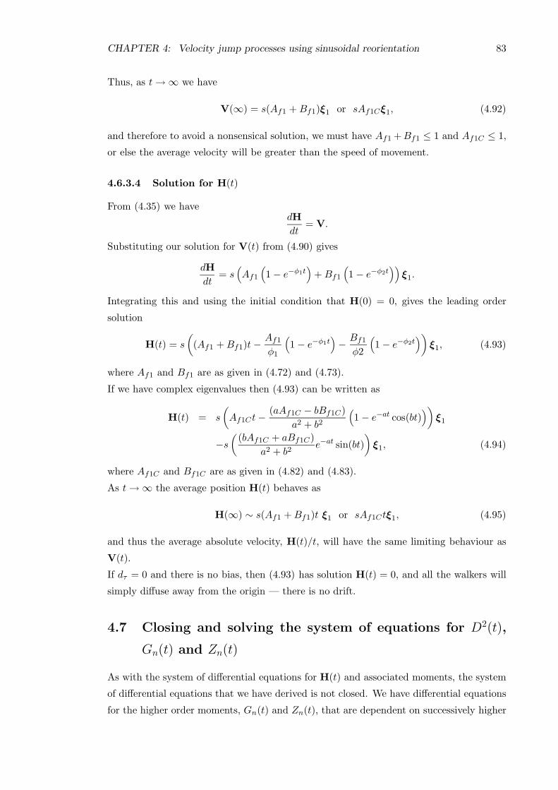
CHAPTER 4: Velocity jump processes using sinusoidal reorientation 83
Thus, as t→ ∞ we have
V(∞) = s(Af1 +Bf1)ξ1 or sAf1Cξ1, (4.92)
and therefore to avoid a nonsensical solution, we must have Af1 +Bf1 ≤ 1 and Af1C ≤ 1,
or else the average velocity will be greater than the speed of movement.
4.6.3.4 Solution for H(t)
From (4.35) we havedH
dt= V.
Substituting our solution for V(t) from (4.90) gives
dH
dt= s
(
Af1
(
1 − e−φ1t)
+Bf1
(
1 − e−φ2t))
ξ1.
Integrating this and using the initial condition that H(0) = 0, gives the leading order
solution
H(t) = s
(
(Af1 +Bf1)t−Af1
φ1
(
1 − e−φ1t)
− Bf1
φ2
(
1 − e−φ2t)
)
ξ1, (4.93)
where Af1 and Bf1 are as given in (4.72) and (4.73).
If we have complex eigenvalues then (4.93) can be written as
H(t) = s
(
Af1Ct−(aAf1C − bBf1C)
a2 + b2
(
1 − e−at cos(bt))
)
ξ1
−s(
(bAf1C + aBf1C)
a2 + b2e−at sin(bt)
)
ξ1, (4.94)
where Af1C and Bf1C are as given in (4.82) and (4.83).
As t→ ∞ the average position H(t) behaves as
H(∞) ∼ s(Af1 +Bf1)t ξ1 or sAf1Ctξ1, (4.95)
and thus the average absolute velocity, H(t)/t, will have the same limiting behaviour as
V(t).
If dτ = 0 and there is no bias, then (4.93) has solution H(t) = 0, and all the walkers will
simply diffuse away from the origin — there is no drift.
4.7 Closing and solving the system of equations for D2(t),
Gn(t) and Zn(t)
As with the system of differential equations for H(t) and associated moments, the system
of differential equations that we have derived is not closed. We have differential equations
for the higher order moments, Gn(t) and Zn(t), that are dependent on successively higher

CHAPTER 4: Velocity jump processes using sinusoidal reorientation 84
order moments. We could carry on deriving differential equations for these successively
higher order moments until we had an extremely large ‘cascade’ of equations. As with
the previous system, in theory this would be possible to solve to a high order as all the
equations are linear, but in practice this is likely to be very complicated.
As with the angular moments, Fn(t) and Yn(t), we would expect the moments Gn(t) and
Zn(t) to get smaller as n increases. Unlike the previous system however, the moments are
dependent on both the angle and position. For n = 1, it is clear that we cannot assume
that the spatial distribution p(x, θ, t) can be split into f(θ)p(x, t), as for example in the
extreme case when the x1 value is very large and negative, it is much more likely that
cos θ is also negative (since in order to reach a point where x1 is large and negative the
walker will have had to move almost directly along an angle close to θ = ±π and hence
cos θ is likely to be negative). For the higher moments (n > 1), this ‘correlation’ between
the angle and spatial position will become weaker and we make a similar approximation
as for the previous system.
4.7.1 Approximating the higher order moments
In a similar way to Section 4.6.1 we assume that for n ≥ 3 we can approximate p(x, θ, t)
by
p(x, θ, t) = f(θ)p(x, t), (4.96)
where f(θ) is the long-time angular distribution given by (4.52), and∫ π
−πf(θ) dθ = 1, and
∫
R2
p(x, t) dx = 1. (4.97)
Thus from (4.16) and (4.18), the higher moments Gn(t) and Zn(t) for n ≥ 3 are given by
Gn(t) =1
N0
∫
R2
(∫ π
−π
cosnθ
2πI0(z)e(z cos θ) dθ
)
x1p(x, t) dx,
Zn(t) =1
N0
∫
R2
(∫ π
−π
sinnθ
2πI0(z)e(z cos θ) dθ
)
x2p(x, t) dx,
and evaluating these using (4.19) and (4.20) gives
Gn(t) =In(z)
I0(z)x1 = An(z)x1, (4.98)
Zn(t) = 0, (4.99)
where x1 = H.ξ1 from (4.48).
To close the systems of equations in (4.47)—(4.51), we use the approximations F3(t) =
A3(z), G3(t) = A3(z)x1, G4(t) = A4(z)x1, and Z3(t) = Z4(t) = 0, where z = −dτ/ ln(A1(κ)).
The differential equations for G1(t) and G2(t), (4.47) and (4.49), can now be written as
dG1
dt=
s
2+s
2F2 − λ11G1 − as1G2 + (as1 + as2A3(z)) x1 + h.o.t., (4.100)
dG2
dt=
s
2F1 +
s
2A3(z) − λ2G2 + bs1G1 +
(
bs2 + bs2A4(z) − bs1A3(z))
x1
+h.o.t., (4.101)

CHAPTER 4: Velocity jump processes using sinusoidal reorientation 85
and similarly for Z1(t) and Z2(t), (4.50) and (4.51) become
dZ1
dt=
s
2− s
2F2 − λ12Z1 − as1Z2 + h.o.t., (4.102)
dZ2
dt=
s
2F1 −
s
2A3(z) − λ2Z2 + bs1Z1 + h.o.t. (4.103)
4.7.2 Solving the final system of equations for D2(t), Gn(t) and Zn(t)
Now that we have closed the original system of equations up to leading order it is straight-
forward to solve.
4.7.2.1 Solving equations for G1(t) and G2(t)
The differential equations in (4.100) and (4.101) form a linear coupled system. Together
with the initial conditions G1(0) = G2(0) = 0 and the solutions from (4.68), (4.69) and
(4.93), this is straightforward to solve using the method described in Section 4.6.2. The
solution for G1(t) to leading order is
G1(t) = s(
(Af1 +Bf1)2t+Ag1
(
1 − e−φ1t)
+Bg1(
1 − e−φ2t)
+ Cg1te−φ1t
+Dg1te−φ2t + Eg1
(
e−φ1t − e−φ2t))
, (4.104)
where
Ag1 = −2A2
f1
φ1−Af1Bf1
(
1
φ1+
1
φ2
)
+(λ2 − φ1)
2φ1(φ2 − φ1)(1 +Af2 +Bf2)
−(λ2 − φ1)(λ2 − φ2)
2bs1φ1(φ2 − φ1)(Af1 +Bf1 +A3(z)) , (4.105)
Bg1 = −2B2
f1
φ2−Af1Bf1
(
1
φ1+
1
φ2
)
− (λ2 − φ2)
2φ2(φ2 − φ1)(1 +Af2 +Bf2)
+(λ2 − φ1)(λ2 − φ2)
2bs1φ2(φ2 − φ1)(Af1 +Bf1 +A3(z)) , (4.106)
Cg1 = A2f1 +
(λ2 − φ1)
2bs1(φ2 − φ1)
(
Af1(λ2 − φ2) −Af2bs1)
, (4.107)
Dg1 = B2f1 −
(λ2 − φ2)
2bs1(φ2 − φ1)
(
Bf1(λ2 − φ1) −Bf2bs1)
, (4.108)
Eg1 = −(λ2 − φ1)
(
bs1(Bf2 − 2Cf1Bf1/φ2) − (λ2 − φ2)(Bf1 − 2Cf2Bf1/φ2))
2bs1(φ2 − φ1)2
+(λ2 − φ2)
(
bs1(Af2 − 2Cf1Af1/φ1) − (λ2 − φ1)(Af1 − 2Cf2Af1/φ1))
2bs1(φ2 − φ1)2,
(4.109)
and φ1, φ2, Af1, Bf1, Af2, and Bf2 are as defined in (4.70) — (4.75).
The solution for G2(t) is of a similar form to (4.104) but is omitted as it is not required
when solving the subsequent differential equations for the spread.
Equation (4.104) gives real-valued solutions if the eigenvalues φi are complex conjugates.

CHAPTER 4: Velocity jump processes using sinusoidal reorientation 86
4.7.2.2 Solving equations for Z1(t) and Z2(t)
The differential equations in (4.102) and (4.103) form a linear coupled system. Together
with the initial conditions Z1(0) = Z2(0) = 0 and the solutions from (4.68) and (4.69),
this is straightforward to solve using the method described in Section 4.6.2. The solution
for Z1(t) to leading order is
Z1(t) = s(
Az1(
1 − e−φ3t)
+Bz1(
1 − e−φ4t)
+ Cz1(
e−φ1t − e−φ3t)
+ Dz1
(
e−φ2t − e−φ3t)
+ Ez1(
e−φ1t − e−φ4t)
+Fz1(
e−φ2t − e−φ4t))
, (4.110)
where
φ3 =1
2
(
λ12 + λ2 −√
(λ12 − λ2)2 − 4as1bs1
)
, (4.111)
φ4 =1
2
(
λ12 + λ2 +√
(λ12 − λ2)2 − 4as1bs1
)
, (4.112)
Az1 =(λ2 − φ3)
2bs1φ3(φ4 − φ3)
(
bs1(1 −Af2 −Bf2) − (λ2 − φ4)(Af1 +Bf1 −A3(z)))
, (4.113)
Bz1 = − (λ2 − φ4)
2bs1φ4(φ4 − φ3)
(
bs1(1 −Af2 −Bf2) − (λ2 − φ3)(Af1 +Bf1 −A3(z)))
, (4.114)
Cz1 =(λ2 − φ3)
2bs1(φ3 − φ1)(φ4 − φ3)
(
bs1Af2 + (λ2 − φ4)Af1
)
, (4.115)
Dz1 =(λ2 − φ3)
2bs1(φ3 − φ2)(φ4 − φ3)
(
bs1Bf2 + (λ2 − φ4)Bf1
)
, (4.116)
Ez1 = − (λ2 − φ4)
2bs1(φ4 − φ1)(φ4 − φ3)
(
bs1Af2 + (λ2 − φ3)Af1
)
, (4.117)
Fz1 = − (λ2 − φ4)
2bs1(φ4 − φ2)(φ4 − φ3)
(
bs1Bf2 + (λ2 − φ3)Bf1
)
, (4.118)
and φ1, φ2, Af1, Bf1, Af2, and Bf2 are as defined in (4.70) — (4.75).
The solution for Z2(t) is of a similar form but is omitted as it is not required when solving
the subsequent differential equations for the spread.
Equation (4.110) gives real-valued solutions if the eigenvalues φi are complex conjugates.
4.7.2.3 Solving equation for D2x1(t)
We havedD2
x1
dt= 2sG1. (4.119)
Substituting for G1(t) from (4.104), integrating, and recalling the initial condition that
D2x1(0) = 0, gives
D2x1(t) = 2s2
(
(Af1 +Bf1)2
2t2 +Ag1
(
t− 1
φ1(1 − e−φ1t)
)
+Bg1
(
t− 1
φ2(1 − e−φ2t)
)

CHAPTER 4: Velocity jump processes using sinusoidal reorientation 87
−Cg1φ1
(
te−φ1t − 1
φ1(1 − e−φ1t)
)
− Dg1
φ2
(
te−φ2t − 1
φ2(1 − e−φ2t)
)
+Eg1
(
1
φ1(1 − e−φ1t) − 1
φ2(1 − e−φ2t)
))
, (4.120)
where the constant terms are as given in (4.105) — (4.109), and φ1, φ2, Af1, Bf1, Af2,
and Bf2 are as defined in (4.70) — (4.75).
As t→ ∞ the spread about the origin in the preferred direction, D2x1(t), behaves as
D2x1(t) ∼ s2(Af1 +Bf1)
2t2, (4.121)
and thus the limiting behaviour of the solution is such that D2x1(t) ∼ t2.
4.7.2.4 Solving equation for D2x2(t)
We havedD2
x2
dt= 2sZ1. (4.122)
Substituting for Z1(t) from (4.110), integrating, and recalling the initial condition that
D2x2(0) = 0, gives
D2x2(t) = 2s2
(
(Az1 +Bz1)t−1
φ3(Az1 + Cz1 +Dz1)
(
1 − e−φ3t)
− 1
φ4(Bz1 +Ez1 + Fz1)
(
1 − e−φ4t)
+1
φ1(Cz1 + Ez1)
(
1 − e−φ1t)
+1
φ2(Dz1 + Fz1)
(
1 − e−φ2t)
)
, (4.123)
where the constant terms are as given in (4.113) — (4.118).
As t→ ∞ the spread about the origin in the non-preferred direction, D2x2(t), behaves as
D2x2(t) ∼ 2s2(Az1 +Bz1)t, (4.124)
and thus the limiting behaviour of the solution is such that D2x2(t) ∼ t — the characteristic
behaviour of a diffusive process.
4.7.2.5 Solving equation for D2(t)
From the definitions in (4.12) — (4.14), we have
D2(t) = D2x1(t) +D2
x2(t), (4.125)
so that the total spread D2(t) is found by adding the equations for the spread in each
direction (4.120) and (4.123).
If dτ = 0 and there is no bias in the system, then the original differential equations for
G1(t) and Z1(t), (4.47) and (4.50), reduce to
dG1
dt=s
2− λ0G1, (4.126)
dZ1
dt=s
2− λ0Z1, (4.127)

CHAPTER 4: Velocity jump processes using sinusoidal reorientation 88
where λ0 = λ(
1 − I1(κ)I0(κ)
)
. This gives the solutions
D2x1(t) = D2
x2(t) =s2
λ0
(
t− 1
λ0(1 − e−λ0t)
)
, (4.128)
and hence the spread about the origin is the same in each direction, and our solution for
D2(t) is the same as in the model of Othmer et al. (1988) with no bias (3.42).
In the absence of bias the spread about the origin in both directions will increase as the
random walk becomes more correlated (κ→ ∞), up to the limiting value of D2(t) = (st)2.
This corresponds to straight line motion directly from the origin along the initial direction
of facing. If bias is present, then this will no longer be true in general as the spread about
the origin will be greater in the preferred direction and if we increase κ to a large enough
value then the spread in the non-preferred direction will start to decrease.
4.7.3 Equations for the spread about the mean position
Now that we have solutions for H(t), D2x1(t) and D2
x2(t) we can solve the equation for
σ2(t). From the definition of σ2x1 and σ2
x2 as the spread about the mean position in the
preferred and non-preferred directions respectively, we have
σ2x1(t) = D2
x1(t) − ‖Hx1(t)‖2, (4.129)
σ2x2(t) = D2
x2(t) − ‖Hx2(t)‖2, (4.130)
where the total spread about the mean position is given by
σ2(t) = σ2x1(t) + σ2
x2(t). (4.131)
4.7.3.1 Equation for σ2x1
The solution for σ2x1 is found by substituting for (4.120) and (4.93) into (4.129). Although
we omit the full solution here, it should be noted that the t2 terms in D2x1(t) and ‖Hx1(t)‖2
cancel so that σ2x1 ∼ t, and the spread about the mean position in the preferred direction
has the characteristic behaviour of a diffusive process (unlike the spread about the origin
in the preferred direction D2x1(t)).
The equation for σ2x1(t) is likely to be highly sensitive to errors in our other equations. For
example, a small relative error in D2x1(t) (which is large) and a small error in H(t) which
is then squared, can result in a large relative error in σ2x1(t). This will occur when the
assumptions we have made about the reorientation parameters being small are no longer
valid.
4.7.3.2 Equation for σ2x2
The mean position in the non-preferred direction has been shown to be zero, Hx2(t) = 0
for all t. Thus the spread about the mean position in the non-preferred direction is the

CHAPTER 4: Velocity jump processes using sinusoidal reorientation 89
same as the spread about the origin in the non-preferred direction,
σ2x2(t) = D2
x2(t). (4.132)
If there is no bias in the system, then the average position H(t) is zero in both directions
and σ2x1 = σ2
x2 = D2x1(t) = D2
x2(t) as given in (4.128).
4.8 Solution plots
Our final solutions for the statistics of interest are of a similar form as the statistic equa-
tions in the model of Othmer et al. (see (3.39)-(3.43)), but with different constant coeffi-
cients and different exponentially decaying terms as we have included higher moments in
our system. The limiting behaviour of our solutions and those of Othmer et al. have the
same form.
The following plots show the general behaviour of the solutions to the equations for the
statistics of interest that we have derived. For each plot we have fixed λ = 1 and s = 1,
and either dτ = 0.1 or dτ = 0.3, and then plotted solutions for κ = 0.1, κ = 1, κ = 2,
κ = 4, and κ = 8 in order to illustrate a wide range of parameter values.
To compare the statistics for the spread in different directions D2x1 and D2
x2, and σ2x1 and
σ2x2, we have plotted solutions for dτ = 0.3 only, as for smaller values of dτ there is less
difference between the spread in each direction.
The plots showing V(t) and H(t) show the expected values for the statistics in the preferred
direction only (x1). The expected values of these statistics in the x2-direction are zero.
4.8.1 Comment on solutions
In general all the plots show sensible behaviour except for the extreme parameter values
in our range — dτ = 0.3 and κ = 8. In this case we start to get nonsensical results —
our assumption that we can round off and/or approximate higher order terms is no longer
valid.
From Figures 4.1 and 4.2, it is clear that the solution for V(t) quickly tends to a fixed
limiting value and H(t) quickly tends to a linear time dependent solution with a fixed
gradient. Both the fixed value for V(t) and the fixed gradient for H(t) are given by
s(Af1 +Bf1) which has a maximum value of 1.
From Figures 4.3 and 4.4, one can see that the solution for D2(t) increases as both κ and
dτ increase, but the solution for σ2(t) decreases as dτ increases, and for dτ = 0.3 starts to
decrease for larger values of κ also. If bias is present, then more of the motion is used to
move in the preferred direction and there is less diffusion away from the mean position.

CHAPTER 4: Velocity jump processes using sinusoidal reorientation 90
k=0.1k=1k=2k=4k=8
0
0.1
0.2
0.3
0.4
0.5
V(t)
20 40 60 80 100
t
(a) dτ = 0.1.
k=0.1k=1k=2k=4k=8
0
0.2
0.4
0.6
0.8
V(t)
20 40 60 80 100
t
(b) dτ = 0.3.
Figure 4.1: Plot of V(t) for dτ = 0.1 and dτ = 0.3 and various values of κ. (The scale of
each plot is different)
k=0.1k=1k=2k=4k=8
0
10
20
30
40
50
H(t)
20 40 60 80 100
t
(a) dτ = 0.1.
k=0.1k=1k=2k=4k=8
0
20
40
60
80
H(t)
20 40 60 80 100
t
(b) dτ = 0.3.
Figure 4.2: Plot of H(t) for dτ = 0.1 and dτ = 0.3 and various values of κ. (The scale of
each plot is different)

CHAPTER 4: Velocity jump processes using sinusoidal reorientation 91
k=0.1k=1k=2k=4k=8
0
1000
2000
3000
4000
20 40 60 80 100
t
(a) dτ = 0.1.
k=0.1k=1k=2k=4k=8
0
1000
2000
3000
4000
5000
6000
7000
20 40 60 80 100
t
(b) dτ = 0.3.
Figure 4.3: Plot of D2(t) for dτ = 0.1 and dτ = 0.3 and various values of κ. (The scale of
each plot is different)
k=0.1k=1k=2k=4k=8
0
200
400
600
800
1000
1200
1400
20 40 60 80 100
t
(a) dτ = 0.1.
k=0.1k=1k=2k=4k=8
0
100
200
300
400
500
20 40 60 80 100
t
(b) dτ = 0.3.
Figure 4.4: Plot of σ2(t) for dτ = 0.1 and dτ = 0.3 and various values of κ. (The scale of
each plot is different)

CHAPTER 4: Velocity jump processes using sinusoidal reorientation 92
k=0.1k=1k=2k=4k=8
0
1000
2000
3000
4000
5000
6000
7000
20 40 60 80 100
t
(a) D2
x1(t).
k=0.1k=1k=2k=4k=8
0
50
100
150
200
250
300
20 40 60 80 100
t
(b) D2
x2(t).
Figure 4.5: Plot of D2x1(t) and D2
x2(t) for dτ = 0.3 and various values of κ. (The scale of
each plot is different)
k=0.1k=1k=2k=4k=8
–50
0
50
100
150
200
250
20 40 60 80 100
t
(a) σ2
x1(t).
k=0.1k=1k=2k=4k=8
0
50
100
150
200
250
300
20 40 60 80 100
t
(b) σ2
x2(t).
Figure 4.6: Plot of σ2x1(t) and σ2
x2(t) for dτ = 0.3 and various values of κ. (The scale of
each plot is different)

CHAPTER 4: Velocity jump processes using sinusoidal reorientation 93
From Figures 4.5 and 4.6, our equations show that the spread will increase as κ increases
for small κ, but for larger values the spread will start to decrease if κ is increased further.
The plot for σ2x1(t) clearly shows that when κ = 8 our model breaks down as, although
we expect a small spread when we have large values for the parameters and ‘straight-line’
motion, it is nonsensical to have ‘negative’ spread. We have already discussed how the
equation for σ2x1(t) is likely to be highly sensitive to errors in the other statistic equations
even if these errors are of a small relative size.
More detailed studies of how accurate these equations are and the effect of the parameters
on the solutions are given in Chapter 6.
4.9 Working with the equations for the statistics of interest
4.9.1 Limitations of the model and solutions
Although we have found some useful general results and we have equations to find the
statistics of interest we should be aware of the assumptions we have made during the
modelling process and how this introduces limitations to the model.
• We have assumed 0 ≤ dτ ≪ 1 so that we ignored some higher order dnτ terms in the
asymptotic expansion. This may make our solutions less accurate as these higher
order terms are not taken into account in the final equations. We would expect our
solutions to become less accurate as the assumption that dτ ≪ 1 becomes less valid
(i.e. if we make dτ large).
• To close the systems of differential equations in (4.40) — (4.50) we first assumed that
the underlying spatial distribution p(x, θ, t) could be approximated by p(x, t)f(θ)
and then approximated the higher moments using the equation for the expected long-
time angular distribution f(θ) from Hill & Hader (1.100). These approximations are
likely to become less valid as the reorientation parameters κ and dτ increase.
• It is clear from solution plots that our solution equations break down for large values
of the parameters κ and dτ due to either or both of the above assumptions. The
equation for σ2x1(t) is highly sensitive to errors in the other equations and we get
nonsensical results for this equation with large values of the parameters.
4.9.2 Rescaling the equations
The equations for the statistics of interest that were derived in the previous section for the
statistics of interest are dependent on time t, and four parameters — the turning frequency
λ, the fixed speed of movement s, and the non-dimensional reorientation parameters κ and

CHAPTER 4: Velocity jump processes using sinusoidal reorientation 94
dτ . The first two parameters can be scaled out of the equations to make them simpler.
The equations will then only be dependent on time and the parameters κ and dτ .
From (4.70), (4.71), (4.111) and (4.112), one can see that the eigenvalues φi are all multi-
ples of λ. It can be seen from (4.72) — (4.75), (4.105) — (4.109) and (4.113) — (4.118)
that the constant terms Af1, Bf1, Af2 and Bf2 are all non-dimensional, while the constant
terms Ag1, Az1 etc are all multiples of 1/λ.
Let us now rewrite φi in the form
φi = λψi for i = 1, 2, 3, 4, (4.133)
and let Ag1 = λAg1, Az1 = λAz1 etc.
We now use the following rescalings
t = λt so t =t
λ,
V(t) = V(t)/s so V(t) = V(t)s,
H(t) = H(t)λ/s so H(t) = H(t)s/λ,
D2x1(t) = D2
x1(t)λ2/s2 so D2
x1(t) = D2x1(t)s
2/λ2,
D2x2(t) = D2
x2(t)λ2/s2 so D2
x2(t) = D2x2(t)s
2/λ2. (4.134)
Using these rescalings, the equation for the average velocity V(t), (4.90), becomes
V(t)s = s(
Af1
(
1 − e−λψ1 t/λ)
+Bf1
(
1 − e−λψ2 t/λ))
ξ1, (4.135)
which simplifies to
V(t) =(
Af1
(
1 − e−ψ1 t)
+Bf1
(
1 − e−ψ2t))
ξ1. (4.136)
In a similar way, the equation for the average position H(t), (4.93), rescales to
H(t) =
(
(Af1 +Bf1)t−Af1
ψ1
(
1 − e−ψ1 t)
− Bf1
ψ2
(
1 − e−ψ2 t)
)
ξ1, (4.137)
and the equations for the spread about the origin in each direction (4.120) and (4.123)
rescale to
D2x1(t) = 2
(
(Af1 +Bf1)2
2t2 + Ag1
(
t− 1
ψ1(1 − e−ψ1 t)
)
+ Bg1
(
t− 1
ψ2(1 − e−ψ2 t)
)
− Cg1ψ1
(
te−ψ1 t − 1
ψ1(1 − e−ψ1 t)
)
− Dg1
ψ2
(
te−ψ2 t − 1
ψ2(1 − e−ψ2 t)
)
+Eg1
(
1
ψ1(1 − e−ψ1 t) − 1
ψ2(1 − e−ψ2 t)
))
, (4.138)
and
D2x2(t) = 2
(
(Az1 + Bz1)t−1
ψ3(Az1 + Cz1 + Dz1)
(
1 − e−ψ3 t)
− 1
ψ4(Bz1 + Ez1 + Fz1)
(
1 − e−ψ4 t)
+1
ψ1(Cz1 + Ez1)
(
1 − e−ψ1 t)
+1
ψ2(Dz1 + Fz1)
(
1 − e−ψ2 t)
)
. (4.139)

CHAPTER 4: Velocity jump processes using sinusoidal reorientation 95
We also define the non-dimensionalised equation for the spread about the mean position
to be
σ2x1(t) = D2
x1(t) − ‖Hx1(t)‖2, (4.140)
σ2x2(t) = D2
x2(t) − ‖Hx2(t)‖2. (4.141)
The rescaled equations can also be obtained by setting the speed to be s = 1 and the
turning frequency to be λ = 1 in the original equations (4.90), (4.93), (4.120) and (4.123),
and changing the time and distance units accordingly.
The non-dimensionalised equations are now dependent on only two parameters — κ and
dτ .
4.9.3 Limits on the parameters
We have observed two possibly unrealistic properties of our solution equations that occur
with large values of the reorientation parameters.
4.9.3.1 Complex eigenvalues
The equations for the spatial statistics derived previously allowed for complex eigenvalues.
The solutions, (4.91) and (4.94), are real valued and there is no reason to assume that they
are not valid. However, it is not clear whether this behaviour is part of the underlying
behaviour of the system, or as seems more likely, is due to the rounding assumptions made
during the derivation of the equations.
From (4.70) and (4.71), the function inside the square root that gives rise to the complex
eigenvalues is given by
ζ1 = (λ11 − λ2)2 − 4as1bs1, (4.142)
where from (4.41) and (4.43) all the constant terms are dependent on the reorientation
parameters κ and dτ . The function ζ1 is of the above form because we have made the
rounding assumptions that dτ is small to enable an asymptotic expansion, and that we
can approximate higher moments as fixed constants using Hill & Hader’s equation for the
long-time angular distribution. With these assumptions we have a closed coupled system
of two differential equations.
Figure 4.7 shows how the non-dimensionalised (s = 1, λ = 1) function ζ1 changes and
becomes negative (resulting in complex eigenvalues), as κ increases for dτ = 0, 0.1, 0.2, 0.3.
Using (4.111) and (4.112), a very similar plot is obtained for φ3 and φ4, where the λ11
terms in (4.142) are replaced by λ12.
From Figure 4.7 it is clear that the larger values of dτ result in complex eigenvalues for
smaller values of κ, while if dτ = 0 the eigenvalues are never complex and ζ1 → 0 as
κ→ ∞.

CHAPTER 4: Velocity jump processes using sinusoidal reorientation 96
d=0d=0.1d=0.2d=0.3
–0.1
–0.05
0
0.05
0.1
0.15
2 4 6 8 10 12 14 16 18 20
k
Figure 4.7: Plot of ζ1 against κ for dτ = 0, 0.1, 0.2, 0.3.
As κ gets larger our assumption that we can approximate the higher order moments such
as Fn(t) for n > 2 will become less valid. All the higher moments Fn → 1 ∀n as κ → ∞.
As dτ gets larger our assumption that dτ ≪ 1 so that we can complete an asymptotic
expansion to a leading order will become less valid.
Thus, it seems likely that the complex eigenvalues that are obtained when we have larger
values of the reorientation parameters are due to the two rounding assumptions made and
are not part of the underlying behaviour of the system, although we have not proved this
to be true.
4.9.3.2 Negative spread
There is no doubt that our solution equation for σ2x1(t) breaks down for larger values of the
reorientation parameters as can be seen in Figure 4.6. Since σ2x1(t) = D2
x1(t) − ‖H(t)‖2,
a small relative error in the equations for H(t) and D2x1 can result in a large error in
σ2x1(t). The errors in the equations are introduced because of the two rounding assumptions
introduced to close the system.
The solution for σ2x1(t) is linear in t and from (4.93) and (4.120), the leading order term
is given by ζ2t where
ζ2 = Ag1 +Bg1 − (Af1 +Bf1)
(
Af1
φ1+Bf1
φ2
)
, (4.143)
and the constants are as defined earlier in (4.72) etc. If ζ2 becomes negative then the long-
time solution for σ2x1(t) will become negative resulting in ‘negative spread’ as discussed
previously and seen in Figure 4.6.

CHAPTER 4: Velocity jump processes using sinusoidal reorientation 97
Figure 4.8 shows how the non-dimensionalised (s = 1, λ = 1) function ζ2 changes and
becomes negative as κ increases for dτ = 0.1, 0.2, 0.3.
d=0.1d=0.2d=0.3
–0.5
0
0.5
1
1.5
2
2.5
3
2 4 6 8 10 12 14 16 18 20
k
Figure 4.8: Plot of ζ2 against κ for dτ = 0.1, 0.2, 0.3.
From Figure 4.8 it is clear that the larger values of dτ result in ‘negative spread’ for
smaller values of κ. Although the exact values of the reorientation parameters do not quite
correspond, there seems to be a parallel between the behaviour shown in Figures 4.7 and
4.8 — some of our equations become unrealistic or nonsensical if we choose reorientation
parameters that are too large.
4.10 Conclusions
We have shown in this chapter that it is possible to extend the velocity jump process
model and method of calculating moments used by Othmer et al. (1988). We have devel-
oped their model by using a reorientation probability distribution based on the von Mises
distribution with mean turning angle given by the sinusoidal reorientation model of Hill &
Hader (1997) that implicitly includes bias. The original probability distributions used by
Othmer et al. were chosen so that a closed system of differential equations was derived for
the moments of the underlying spatial distribution (see Chapter 3). When using a more re-
alistic reorientation probability distribution that includes sinusoidal reorientation, we have
shown in our analysis that the system of differential equations derived for the moments
of the spatial distribution is not closed, even when working to leading order by assuming
that the reorientation parameter dτ is small. We are able to close the system of differen-
tial equations by approximating the higher order moments using Hill & Hader’s equation
for the expected long-time angular distribution (1.100), and making an assumption about

CHAPTER 4: Velocity jump processes using sinusoidal reorientation 98
the underlying spatial distribution. This results in a system of equations for the spatial
statistics (V(t), H(t), D2(t) and σ2(t)) of the population of random walkers that are valid
for all time and not just long-time approximations as in the diffusion model. Othmer et
al. did not derive equations for the spread in each direction, but we have extended the
analysis to include equations for D2x1(t), D
2x2(t), σ
2x1(t) and σ2
x2(t). The equations for the
spatial statistics are dependent on the turning frequency λ, the fixed speed of movement
s, and the reorientation parameters κ and dτ . Using suitable rescalings the equations can
be non-dimensionalised to be dependent on the reorientation parameters only. Because of
the various assumptions made during the analysis, the equations are not valid over all the
parameter space for κ and dτ , and if both are ‘large’ then the equations underestimate
the spread about the mean position, or give the nonsensical result of ‘negative spread.’
The sinusoidal reorientation model is motivated by the gyrotactic movement of algae such
as C. nivalis under a gravitational torque, but the model and solution equations presented
in this chapter could be used to describe the movement of any random walker moving in
a homogenous environment with sinusoidal reorientation.
The main results of this chapter are summarised below:
• We have developed the velocity jump process of Othmer et al. to include a realistic
reorientation probability distribution that implicitly introduces bias to the movement
by including the dependence of the mean turning angle on the sine of the absolute
angle (sinusoidal reorientation model) from Hill & Hader’s experimental results.
• We have derived equations for the statistics of the underlying spatial distribution
that are valid for all time, these statistics being the mean velocity V(t), the mean
position H(t), the spread about the origin D2(t) and the spread about the mean
position σ2(t).
• We also have equations that are valid for all time for the spread in each of the
preferred and non-preferred directions, D2x1(t), D
2x2(t), σ
2x1(t) and σ2
x2(t).
• To close and solve the system of differential equations we had to make certain as-
sumptions about the reorientation parameters and the properties of the higher mo-
ments. We assumed that the parameter dτ was small to allow Taylor expansions of
the trigonometric functions and so all the equations are only leading order approxi-
mations. We also approximated the higher moments using Hill & Hader’s equation
for the expected long-time angular distribution in order to close the final system of
differential equations.
• Because of these assumptions, the equations for the spatial statistics are not valid
for large values of the reorientation parameters to avoid nonsensical results.

Chapter 5
Velocity jump processes using
linear reorientation
5.1 Introduction
In the previous chapter we have shown how it is possible to extend the velocity jump
process and method of calculating moments used by Othmer et al. (1988) to include a
reorientation distribution, T (θ, θ′), that has a mean turning angle given by the sinusoidal
reorientation model of Hill & Hader (1997). After analysing data from experiments on
algae, Hill & Hader suggested that the mean turning angle is dependent on the absolute
direction, and showed how this results in two models for reorientation — sinusoidal and
linear (Section 1.5). Linear reorientation has been observed in algae such as C. nivalis or
P. gatunese that move towards or away from light, a process known as phototaxis, see for
example Hill & Vincent (1993) and Vincent & Hill (1996). In this chapter we develop the
velocity jump process model and method of calculating the moments used by Othmer et
al. (1988) to derive equations for the moments of the underlying spatial distribution of
a population moving with a reorientation distribution, T (θ, θ′), that has a mean turning
angle given by Hill & Hader’s linear reorientation model.
5.2 Results and assumptions to be used in analysis
5.2.1 Reorientation model
As discussed in the introductory chapter, when looking at the trajectories of swimming
micro-organisms such as C. nivalis, Hill & Hader (1997) derived a probability distribution
function for the orientation of the cells, from which certain parameters can be calculated.
After analysing experimental results they showed that the mean turning angle is dependent
99

CHAPTER 5: Velocity jump processes using linear reorientation 100
on the direction of movement and for phototaxis is given by
µδ(θ) =
−B−1τθ, −π < θ < π,
0, θ = ±π,(5.1)
from (1.87) and (1.101), where τ is the average time between turns, B is the average
reorientation time and θ0 = 0 is the preferred direction. We define dτ and κ in the same
way as in the sinusoidal model (see (4.2) and (4.6)). We assume that the taxis is positive
(i.e. individuals prefer to move towards the light source), and that the amplitude of the
reorientation coefficient B−1 is fixed and not dependent on the spatial position. As in
the sinusoidal model, the symmetric probability distribution we use for the reorientation
distribution is the von Mises distribution (see Section 1.2.3.2).
To model the linear reorientation observed in phototaxis using the velocity jump process
model of Othmer et al. we substitute for Hill & Hader’s µδ = −dτθ (assuming that θ0 = 0
for convenience) and recognise that if we define δ = θ− θ′, the von Mises distribution f(δ)
can be used as the reorientation kernel T (θ, θ′). This gives
T (θ, θ′) =1
2πI0(κ)eκ cos(θ−θ′+dτ θ′) (5.2)
where∫ π
−πT (θ, θ′) dθ = 1.
Thus we have a probability distribution for reorientation that implicitly includes bias. We
now extend the velocity jump process model of Othmer at al. (1988) using our probability
distribution for reorientation that implicitly includes bias.
5.2.2 Defining higher order moments
The statistics of interest are the mean location of cells H(t), their mean squared displace-
ment D2(t), and their mean velocity V(t), which are defined as in (4.10)—(4.12). We also
derive equations for the statistics of the spread in each direction D2x1(t) and D2
x2(t) which
are defined in (4.13) and (4.14). In addition we recall the definition of σ2(t) (3.20).
We introduce the following extra auxiliary functions
Fn(t) =1
N0
∫
R2
∫ π
−πcosnθ p(x, θ, t) dθ dx, (5.3)
Yn(t) =1
N0
∫
R2
∫ π
−πsinnθ p(x, θ, t) dθ dx, (5.4)
Kn(t) =1
N0
∫
R2
∫ π
−πθ sinnθ p(x, θ, t) dθ dx, (5.5)
Ln(t) =1
N0
∫
R2
∫ π
−πθ cosnθ p(x, θ, t) dθ dx, (5.6)
Mn(t) =1
N0
∫
R2
∫ π
−πθ2 cosnθ p(x, θ, t) dθ dx, (5.7)
Nn(t) =1
N0
∫
R2
∫ π
−πθ2 sinnθ p(x, θ, t) dθ dx, (5.8)

CHAPTER 5: Velocity jump processes using linear reorientation 101
Gn(t) =1
N0
∫
R2
∫ π
−πx1 cosnθ p(x, θ, t) dθ dx, (5.9)
Zn(t) =1
N0
∫
R2
∫ π
−πx2 sinnθ p(x, θ, t) dθ dx, (5.10)
Pn(t) =1
N0
∫
R2
∫ π
−πx1θ sinnθ p(x, θ, t) dθ dx, (5.11)
Qn(t) =1
N0
∫
R2
∫ π
−πx2θ cosnθ p(x, θ, t) dθ dx, (5.12)
Rn(t) =1
N0
∫
R2
∫ π
−πx1θ
2 cosnθ p(x, θ, t) dθ dx, (5.13)
Sn(t) =1
N0
∫
R2
∫ π
−πx2θ
2 sinnθ p(x, θ, t) dθ dx, (5.14)
which will be used in the subsequent analysis. The higher moments Fn(t), Gn(t), Yn(t)
and Zn(t) were used in the sinusoidal model and have been discussed previously. The
other moments are dependent on the functions θ sinnθ, θ cosnθ, θ2 cosnθ and θ2 sinnθ.
As in the sinusoidal model, we assume that all the population starts at the origin (0, 0)
and that the initial directions are equally distributed around the unit circle. Using this
assumption
Fn(0) = Gn(0) = Yn(0) = Zn(0) = 0,
and
Pn(0) = Qn(0) = Rn(0) = Sn(0) = 0.
The initial conditions for Kn(0), Ln(0), Mn(0) and Nn(0) are straightforward to derive.
If we start at the origin with an equal spread of directions then p(0, θ, 0) = 1/2π, and so
we have
K1(0) =1
N0
∫
R2
∫ π
−π
θ sin θ
2πdθ dx = 1,
L1(0) =1
N0
∫
R2
∫ π
−π
θ cos θ
2πdθ dx = 0,
M1(0) =1
N0
∫
R2
∫ π
−π
θ2 cos θ
2πdθ dx = −2.
N1(0) =1
N0
∫
R2
∫ π
−π
θ2 sin θ
2πdθ dx = 0,
K2(0) =1
N0
∫
R2
∫ π
−π
θ sin 2θ
2πdθ dx = −1
2,
L2(0) =1
N0
∫
R2
∫ π
−π
θ cos 2θ
2πdθ dx = 0,
M2(0) =1
N0
∫
R2
∫ π
−π
θ2 cos 2θ
2πdθ dx =
1
2,
and N2(0) =1
N0
∫
R2
∫ π
−π
θ2 sin 2θ
2πdθ dx = 0.
All other statistics we are interested in are assumed to be 0 at t = 0.

CHAPTER 5: Velocity jump processes using linear reorientation 102
5.2.3 Integrals of the von Mises distribution
From (4.23) and (4.24), we use the following identities for the integrals of the modified
von Mises distribution∫ π
−π
cos pθ
2πI0(κ)eκ cos(θ−θ′+dτ θ′) dθ =
Ip(κ)
I0(κ)cos(pθ′ − pdτθ
′) (5.15)
∫ π
−π
sin pθ
2πI0(κ)eκ cos(θ−θ′+dτ θ′) dθ =
Ip(κ)
I0(κ)sin(pθ′ − pdτθ
′). (5.16)
5.2.4 Asymptotic expansions of the trigonometric functions
We assume that 0 ≤ dτ ≪ 1, and seek an asymptotic expansion in powers of dτ for the
trigonometric functions.
The standard Taylor Series expansions for the trigonometric functions that will be needed
in the later analysis are:
cos(nθ − ndτθ) = cosnθ + ndτθ sinnθ − n2d2τ
2θ2 cosnθ +O(d3
τ ) (5.17)
sin(nθ − ndτθ) = sinnθ − ndτθ cosnθ − n2d2τ
2θ2 sinnθ +O(d3
τ ). (5.18)
Using the standard trigonometric identities, (5.17) and (5.18) reduce for n = 1 and n = 2
to
cos(θ − dτθ) = cos θ + dτθ sin θ − d2τ
2θ2 cos θ +O(d3
τ ), (5.19)
cos(2θ − 2dτθ) = cos 2θ + 2dτθ sin 2θ − 2d2τθ
2 cos 2θ +O(d3τ ), (5.20)
sin(θ − dτθ) = sin θ − dτθ cos θ − d2τ
2θ2 sin θ +O(d3
τ ), (5.21)
sin(2θ − 2dτθ) = sin 2θ − 2dτθ cos 2θ − 2d2τθ
2 sin 2θ +O(d3τ ). (5.22)
5.2.5 Previous results
• As in the previous chapters (see Section 3.3.2.1), we assume that we can change the
order of integration between dx, dθ and dθ′.
• As in the previous chapters (see Section 3.3.2.2), we use the divergence theorem to
show that the following integrals hold∫
R2
−a(ξ.∇xp) dx =
∫
R2
pξ.(∇xa) dx, (5.23)
for scalar functions a, and∫
R2
−v(ξ.∇xp) dx =
∫
R2
(p(ξ.∇x)v) dx, (5.24)
for vector functions v.
• Also, for convenience in the subsequent calculations, we shall write p(θ) or p in place
of p(θ,x, t).

CHAPTER 5: Velocity jump processes using linear reorientation 103
5.3 Differential equations for the spatial statistics and higher
order moments
Using a similar method to Othmer et al. (1988), differential equations for the statistics
of interest and higher moments can be derived using the evolution equation given earlier
(3.11).
5.3.1 Deriving equations for spatial statistics
5.3.1.1 Differential equation for H(t)
In the previous chapters the differential equation derived for H(t) (see (3.28)), was in-
dependent of the choice of T (θ, θ′), and so the equation for H(t) for the case of linear
re-orientation will be the same, i.e.dH
dt= V. (5.25)
5.3.1.2 Differential equation for V(t)
From the definitions of F1(t) and Y1(t) in (5.3) and (5.4) respectively, we have
V(t) = s(F1(t), Y1(t)), (5.26)
and thus it is not necessary to derive a differential equation for V(t) directly if we are able
to find solutions for F1(t) and Y1(t).
5.3.1.3 Differential equation for D2(t)
From the definitions of D2x1(t) and D2
x2(t) in (4.13) and (4.14) respectively, we have
D2(t) = D2x1(t) +D2
x2(t), (5.27)
and thus it is not necessary to derive a differential equation for D2(t) directly if we are
able to find solutions for D2x1(t) and D2
x2(t).
5.3.1.4 Differential equation for D2x1(t)
In the previous chapter the differential equation derived for D2x1(t) (see (4.38)), was in-
dependent of the choice of T (θ, θ′), and so the equation for D2x1(t) for the case of linear
re-orientation will be the samedD2
x1
dt= 2sG1, (5.28)
where G1 is defined in (5.9).

CHAPTER 5: Velocity jump processes using linear reorientation 104
5.3.1.5 Differential equation for D2x2(t)
In the previous chapter the differential equation derived for D2x2(t) (see (4.39)), was in-
dependent of the choice of T (θ, θ′), and so the equation for D2x2(t) for the case of linear
re-orientation will be the samedD2
x2
dt= 2sZ1, (5.29)
where Z1 is defined in (5.10).
5.3.1.6 Equation for σ2(t)
We also have the equation derived earlier for σ2(t) (see (3.43)),
σ2(t) = D2(t) − ‖H(t)‖2, (5.30)
and the corresponding equations for the spread in each direction
σ2x1(t) = D2
x1(t) − ‖Hx1(t)‖2, (5.31)
and σ2x2(t) = D2
x2(t) − ‖Hx2(t)‖2. (5.32)
5.3.2 Deriving equations for the higher order moments
5.3.2.1 Estimating the integrals
To derive differential equations for all the following higher order moments it is necessary
to solve the following integrals
kn(µ, κ) =
∫ π
−πθ sinnθ eκ cos(θ−µ) dθ, (5.33)
ln(µ, κ) =
∫ π
−πθ cosnθ eκ cos(θ−µ) dθ, (5.34)
mn(µ, κ) =
∫ π
−πθ2 cosnθ eκ cos(θ−µ) dθ , (5.35)
and
nn(µ, κ) =
∫ π
−πθ2 sinnθ eκ cos(θ−µ) dθ , (5.36)
for n = 1 and 2, and where µ = θ′ − dτθ′.
These integrals are then multiplied by p(θ′) and integrated over dθ′ and dx to give differ-
ential equations for the moments of the population distribution.
While it is possible to solve the integrals numerically for fixed parameter values, we are
unable to solve these integrals in an analytic way. It should be noted that even if an
analytic solution exists, the final solutions will still only be leading order approximations
due to the assumption we have made that dτ ≪ 1. As we are able to evaluate the integrals
numerically, we fit simple known functions (dependent on µ and κ), to allow us to make
further analytical progress.

CHAPTER 5: Velocity jump processes using linear reorientation 105
5.3.2.2 Fitting a function to integral (5.33) with n = 1
By inspection we fitted functions of Bessel functions to plots of the integral that had been
evaluated for fixed values of the parameter κ. We found that as κ increases, increasingly
complex terms involving higher order Bessel functions are needed to obtain a good fit. To
avoid over-complication, the function
k1(µ, κ) = 2πI0(κ) − πI1(κ) cos µ− πI2(κ) cos 2µ, (5.37)
was used to approximate (5.33) with n = 1. Plots comparing the function k1(µ, κ) to the
exact integral for |µ| ≤ π, are shown for various values of κ in Figure 5.1.
Note that when κ = 0, both the exact integral and the test function k1(µ, κ) equal 2π.
This function is a good fit for small values of the parameter κ but becomes increasingly
less of a fit as κ gets larger.
5.3.2.3 Fitting functions to the further integrals
Similarly, we fitted the following functions to the integrals given in (5.33) — (5.36) re-
spectively, for n = 1 and n = 2.
l1(µ, κ) = −I1(κ)π sinµ+ 2I2(κ)π sin 2µ, (5.38)
m1(µ, κ) = −4πI0(κ) + 8πI1(κ) cos µ− 4πI2(κ) cos 2µ, (5.39)
n1(µ, κ) = 6πI1(κ) sinµ, (5.40)
k2(µ, κ) = −πI0(κ) + 3πI1(κ) cos µ− 3
2πI2(κ) cos 2µ, (5.41)
l2(µ, κ) = −3
2I1(κ)π sinµ− I2(κ)π sin 2µ, (5.42)
m2(µ, κ) = πI0(κ) − 4πI1(κ) cos µ+ 6πI2(κ) cos 2µ, (5.43)
n2(µ, κ) = −4πI1(κ) sinµ+ 8πI2(κ) sin 2µ. (5.44)
Plots comparing the functions defined above, (5.38) — (5.44) to the exact integrals for
|µ| ≤ π, are shown for various values of κ in Figures 5.2 — 5.8.
5.3.2.4 Comment on the fitted functions
The functions (5.37)—(5.44) are used to approximate the integrals (5.33)—(5.36) with
n = 1 and 2, in the subsequent analysis.
The method of estimating the exact integrals (5.33)—(5.36) by fitting simple functions that
approximate the solution could be considered quite crude, and more sophisticated ways
may possibly be found to calculate better approximations or even the exact solutions.
However, it should be noted that even if we had exact solutions to these integrals our final
differential equations will still only be approximations themselves due to the assumptions
we make in working to a leading order and assuming O(d3τ ) terms are negligible. As
we are aware that our final differential equations and solutions will only be leading order

CHAPTER 5: Velocity jump processes using linear reorientation 106
Test function k1Exact integral
Legend
5.8
6
6.2
6.4
6.6
6.8
7
7.2
7.4
–3 –2 –1 0 1 2 3µ
(a) κ = 0.5.
Test function k1Exact integral
Legend
6
6.5
7
7.5
8
8.5
9
–3 –2 –1 0 1 2 3µ
(b) κ = 1.
Test function k1Exact integral
Legend
8
10
12
14
16
18
–3 –2 –1 0 1 2 3µ
(c) κ = 2.
Test function k1Exact integral
Legend
20
40
60
80
100
–3 –2 –1 0 1 2 3µ
(d) κ = 4.
Figure 5.1: Plots comparing k1(µ, κ) to the exact integral for various values of κ. (The
scale of each plot is different).

CHAPTER 5: Velocity jump processes using linear reorientation 107
Test function l1Exact integral
Legend
–0.8
–0.6
–0.4
–0.2
0
0.2
0.4
0.6
0.8
–3 –2 –1 1 2 3µ
(a) κ = 0.5.
Test function l1Exact integral
Legend
–2
–1
0
1
2
–3 –2 –1 1 2 3µ
(b) κ = 1.
Test function l1Exact integral
Legend
–10
–5
5
10
–3 –2 –1 1 2 3µ
(c) κ = 2.
Test function l1Exact integral
Legend
–80
–60
–40
–20
0
20
40
60
80
–3 –2 –1 1 2 3µ
(d) κ = 4.
Figure 5.2: Plots comparing l1(µ, κ) to the exact integral for various values of κ. (The
scale of each plot is different).
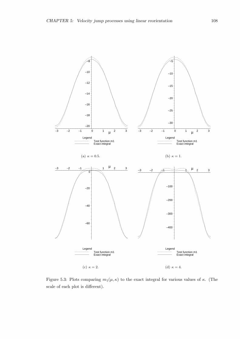
CHAPTER 5: Velocity jump processes using linear reorientation 108
Test function m1Exact integral
Legend
–20
–18
–16
–14
–12
–10
–8
–3 –2 –1 0 1 2 3µ
(a) κ = 0.5.
Test function m1Exact integral
Legend
–30
–25
–20
–15
–10
–5
–3 –2 –1 0 1 2 3µ
(b) κ = 1.
Test function m1Exact integral
Legend
–60
–40
–20
0–3 –2 –1 1 2 3µ
(c) κ = 2.
Test function m1Exact integral
Legend
–400
–300
–200
–100
–3 –2 –1 1 2 3µ
(d) κ = 4.
Figure 5.3: Plots comparing m1(µ, κ) to the exact integral for various values of κ. (The
scale of each plot is different).

CHAPTER 5: Velocity jump processes using linear reorientation 109
Test function n1Exact integral
Legend
–4
–2
0
2
4
–3 –2 –1 1 2 3µ
(a) κ = 0.5.
Test function n1Exact integral
Legend
–10
–5
0
5
10
–3 –2 –1 1 2 3µ
(b) κ = 1.
Test function n1Exact integral
Legend
–30
–20
–10
10
20
30
–3 –2 –1 1 2 3µ
(c) κ = 2.
Test function n1Exact integral
Legend
–200
–100
0
100
200
–3 –2 –1 1 2 3µ
(d) κ = 4.
Figure 5.4: Plots comparing n1(µ, κ) to the exact integral for various values of κ. (The
scale of each plot is different).

CHAPTER 5: Velocity jump processes using linear reorientation 110
Test function k2Exact integral
Legend
–5
–4
–3
–2
–1
–3 –2 –1 0 1 2 3µ
(a) κ = 0.5.
Test function k2Exact integral
Legend
–10
–8
–6
–4
–2
–3 –2 –1 1 2 3µ
(b) κ = 1.
Test function k2Exact integral
Legend
–25
–20
–15
–10
–5
0
5
–3 –2 –1 1 2 3µ
(c) κ = 2.
Test function k2Exact integral
Legend
–160
–140
–120
–100
–80
–60
–40
–20
20
–3 –2 –1 1 2 3µ
(d) κ = 4.
Figure 5.5: Plots comparing k2(µ, κ) to the exact integral for various values of κ. (The
scale of each plot is different).

CHAPTER 5: Velocity jump processes using linear reorientation 111
Test function l2Exact integral
Legend
–1
–0.5
0
0.5
1
–3 –2 –1 1 2 3µ
(a) κ = 0.5.
Test function l2Exact integral
Legend
–2
–1
0
1
2
–3 –2 –1 1 2 3µ
(b) κ = 1.
Test function l2Exact integral
Legend
–8
–6
–4
–2
0
2
4
6
8
–3 –2 –1 1 2 3µ
(c) κ = 2.
Test function l2Exact integral
Legend
–60
–40
–20
0
20
40
60
–3 –2 –1 1 2 3µ
(d) κ = 4.
Figure 5.6: Plots comparing l2(µ, κ) to the exact integral for various values of κ. (The
scale of each plot is different).
CHAPTER 5: Velocity jump processes using linear reorientation 112
Test function m2Exact integral
Legend
1
2
3
4
5
6
7
–3 –2 –1 0 1 2 3µ
(a) κ = 0.5.
Test function m2Exact integral
Legend
2
4
6
8
10
12
14
–3 –2 –1 1 2 3µ
(b) κ = 1.
Test function m2Exact integral
Legend
–10
0
10
20
30
40
–3 –2 –1 1 2 3µ
(c) κ = 2.
Test function m2Exact integral
Legend
–100
0
100
200
300
–3 –2 –1 1 2 3µ
(d) κ = 4.
Figure 5.7: Plots comparing m2(µ, κ) to the exact integral for various values of κ. (The
scale of each plot is different).

CHAPTER 5: Velocity jump processes using linear reorientation 113
Test function n2Exact integral
Legend
–3
–2
–1
0
1
2
3
–3 –2 –1 1 2 3µ
(a) κ = 0.5.
Test function n2Exact integral
Legend
–8
–6
–4
–2
0
2
4
6
8
–3 –2 –1 1 2 3µ
(b) κ = 1.
Test function n2Exact integral
Legend
–30
–20
–10
10
20
30
–3 –2 –1 1 2 3µ
(c) κ = 2.
Test function n2Exact integral
Legend
–200
–100
100
200
–3 –2 –1 1 2 3µ
(d) κ = 4.
Figure 5.8: Plots comparing n2(µ, κ) to the exact integral for various values of κ. (The
scale of each plot is different).

CHAPTER 5: Velocity jump processes using linear reorientation 114
approximations to the true solutions, this method of estimating the exact integrals with the
fitted functions is reasonable. The final solutions are validated by comparing to numerical
simulations in Chapter 6.
5.3.2.5 Differential equation for F1(t)
Multiply the original linear transport equation (3.11) by cos θ, integrate over θ and x, and
divide by N0, to give
1
N0
∫
R2
∫ π
−πcos θ
∂p
∂tdθ dx =
s
N0
∫
R2
∫ π
−πcos θ (ξ.∇
xp) dθ dx
− λ
N0
∫
R2
∫ π
−πcos θ p dθ dx
+λ
N0
∫
R2
∫ π
−π
∫ π
−πcos θ T (θ, θ′) p(θ′) dθ′ dθ dx.
The first term in the right hand side of the above is zero due to the divergence theorem
(see Section 3.3.2.2). Substituting for F1(t) from (5.3) and for T (θ, θ′) from (5.2), gives
dF1
dt= −λF1 +
λ
2πI0(κ)N0
∫
R2
∫ π
−π
∫ π
−πcos θ eκ cos(θ−µ) p(θ′) dθ′ dθ dx,
where µ = θ′ − dτθ′.
The order of the integral in the above can be changed (see Section 3.3.2.1), and then using
(5.15) we get
dF1
dt= −λF1 +
λI1(κ)
I0(κ)N0
∫
R2
∫ π
−πcos(θ′ − dτθ
′) p(θ′) dθ′ dx.
Expanding this using the Taylor Series expansion of the trigonometric functions (5.19)
and then substituting using the definitions of the higher moments given in (5.3) — (5.14),
givesdF1
dt= −λ
(
1 − I1(κ)
I0(κ)
)
F1 +dτλI1(κ)
I0(κ)K1 −
d2τλI1(κ)
2I0(κ)M1 +O(d3
τ ). (5.45)
5.3.2.6 Differential equation for K1(t)
Recalling the definition of K1(t) from (5.5) and using the same method as in Section
5.3.2.5, we get
dK1
dt= −λK1 +
λ
2πI0(κ)N0
∫
R2
∫ π
−π
∫ π
−πθ sin θ eκ cos(θ−µ) p(θ′) dθ′ dθ dx,
where µ = θ′ − dτθ′.
The order of the integral in the above can be changed (see Section 3.3.2.1), and then using
(5.37) and substituting for µ we get
dK1
dt= −λK1 +
λ
2πI0(κ)N0
∫
R2
∫ π
−π(2πI0(κ) − πI1(κ) cos(θ′ − dτθ
′)) p(θ′) dθ′ dx
− λ
2πI0(κ)N0
∫
R2
∫ π
−π(πI2(κ) cos(2θ′ − 2dτθ
′)) p(θ′) dθ′ dx,

CHAPTER 5: Velocity jump processes using linear reorientation 115
Expanding this using the Taylor Series expansion of the trigonometric functions (5.19)
and (5.20), and then substituting using the definitions of the higher moments given in
(5.3) — (5.14), gives
dK1
dt= −λ
(
1 +dτI1(κ)
2I0(κ)
)
K1 + λ− λI1(κ)
2I0(κ)F1
+λI1(κ)d
2τ
4I0(κ)M1 −
λI2(κ)
2I0(κ)F2 −
λI2(κ)dτI0(κ)
K2 +λI2(κ)d
2τ
I0(κ)M2 +O(d3
τ ). (5.46)
5.3.2.7 Differential equation for M1(t)
Recalling the definition of M1(t) from (5.7) and using the same method as in Section
5.3.2.5, we get
dM1
dt= −λM1 +
λ
2πI0(κ)N0
∫
R2
∫ π
−π
∫ π
−πθ2 cos θ eκ cos(θ−µ) p(θ′) dθ′ dθ dx,
where µ = θ′ − dτθ′.
The order of the integral in the above can be changed (see Section 3.3.2.1), and then using
(5.39) and substituting for µ we get
dM1
dt= −λM1 +
λ
2πI0(κ)N0
∫
R2
∫ π
−π(−4πI0(κ) + 8πI1(κ) cos(θ′ − dτθ
′)) p(θ′) dθ′ dx
− λ
2πI0(κ)N0
∫
R2
∫ π
−π(4πI2(κ) cos(2θ′ − 2dτθ
′)) p(θ′) dθ′ dx,
Expanding this using the Taylor Series expansion of the trigonometric functions (5.19)
and (5.20), and then substituting using the definitions of the higher moments given in
(5.3) — (5.14), gives
dM1
dt= −λ
(
1 +2d2τ I1(κ)
I0(κ)
)
M1 − 2λ+4λI1(κ)
I0(κ)F1 +
4λI1(κ)dτI0(κ)
K1
−2λI2(κ)
I0(κ)F2 −
4λI2(κ)dτI0(κ)
K2 +4λI2(κ)d
2τ
I0(κ)M2 +O(d3
τ ). (5.47)
5.3.2.8 Differential equation for F2(t)
Recalling the definition of F2(t) from (5.3) and using the same method as in Section 5.3.2.5,
we get
dF2
dt= −λF2 +
λ
2πI0(κ)N0
∫
R2
∫ π
−π
∫ π
−πcos 2θ eκ cos(θ−µ) p(θ′) dθ′ dθ dx,
where µ = θ′ − dτθ′.
The order of the integral in the above can be changed (see Section 3.3.2.1), and then using
(5.15) and substituting for µ we get
dF2
dt= −λF2 +
λI2(κ)
I0(κ)N0
∫
R2
∫ π
−π
∫ π
−πcos(2θ′ − 2dτθ
′)) p(θ′) dθ′ dθ dx,

CHAPTER 5: Velocity jump processes using linear reorientation 116
Expanding this using the Taylor Series expansion of the trigonometric functions (5.20)
and then substituting using the definitions of the higher moments given in (5.3) — (5.14),
gives
dF2
dt= −λ
(
1 − I2(κ)
I0(κ)
)
F2 +2λI2(κ)dτI0(κ)
K2 −2λI2(κ)d
2τ
I0(κ)M2 +O(d3
τ ). (5.48)
5.3.2.9 Differential equation for K2(t)
Recalling the definition of K2(t) from (5.5) and using the same method as in Section
5.3.2.5, we get
dK2
dt= −λK2 +
λ
2πI0(κ)N0
∫
R2
∫ π
−π
∫ π
−πθ sin 2θ eκ cos(θ−µ) p(θ′) dθ′ dθ dx,
where µ = θ′ − dτθ′.
The order of the integral in the above can be changed (see Section 3.3.2.1), and then using
(5.41) and substituting for µ we get
dK2
dt= −λK2 +
λ
2πI0(κ)N0
∫
R2
∫ π
−π(−πI0(κ) + 3πI1(κ) cos(θ′ − dτθ
′)) p(θ′) dθ′ dθ dx
− λ
2πI0(κ)N0
∫
R2
∫ π
−π(3
2πI2(κ) cos(2θ′ − 2dτθ
′)) p(θ′) dθ′ dθ dx,
Expanding this using the Taylor Series expansion of the trigonometric functions (5.19)
and (5.20), and then substituting using the definitions of the higher moments given in
(5.3) — (5.14), gives
dK2
dt= −λ
(
1 +3dτ I2(κ)
2I0(κ)
)
K2 −λ
2+
3λI1(κ)
2I0(κ)F1 +
3λI1(κ)dτ2I0(κ)
K1
−3λI1(κ)d2τ
4I0(κ)M1 −
3λI2(κ)
4I0(κ)F2 +
3λI2(κ)d2τ
2I0(κ)M2 +O(d3
τ ). (5.49)
5.3.2.10 Differential equation for M2(t)
Recalling the definition of M2(t) from (5.7) and using the same method as in Section
5.3.2.5, we get
dM2
dt= −λM2 +
λ
2πI0(κ)N0
∫
R2
∫ π
−π
∫ π
−πθ2 cos 2θ eκ cos(θ−µ) p(θ′) dθ′ dθ dx,
where µ = θ′ − dτθ′.
The order of the integral in the above can be changed (see Section 3.3.2.1), and then using
(5.43) and substituting for µ we get
dM2
dt= −λM2 +
λ
2πI0(κ)N0
∫
R2
∫ π
−π(πI0(κ) − 4πI1(κ) cos(θ′ − dτθ
′)) p(θ′) dθ′ dθ dx
+λ
2πI0(κ)N0
∫
R2
∫ π
−π(6πI2(κ) cos(2θ′ − 2dτθ
′)) p(θ′) dθ′ dθ dx,

CHAPTER 5: Velocity jump processes using linear reorientation 117
Expanding this using the Taylor Series expansion of the trigonometric functions (5.19)
and (5.20), and then substituting using the definitions of the higher moments given in
(5.3) — (5.14), gives
dM2
dt= −λ
(
1 +6d2τ I2(κ)
I0(κ)
)
M2 +λ
2− 2λI1(κ)
I0(κ)F1 −
2λI1(κ)dτI0(κ)
K1
+λI1(κ)d
2τ
I0(κ)M1 +
3λI2(κ)
I0(κ)F2 +
6λI2(κ)dτI0(κ)
K2 +O(d3τ ). (5.50)
5.3.2.11 Differential equation for Y1(t)
Recalling the definition of Y1(t) from (5.4) and using the same method as in Section 5.3.2.5,
we get
dY1
dt= −λY1 +
λ
2πI0(κ)N0
∫
R2
∫ π
−π
∫ π
−πsin θ eκ cos(θ−µ) p(θ′) dθ′ dθ dx,
where µ = θ′ − dτθ′.
The order of the integral in the above can be changed (see Section 3.3.2.1), and then using
(5.16) and substituting for µ we get
dY1
dt= −λY1 +
λI1(κ)
I0(κ)N0
∫
R2
∫ π
−π
∫ π
−πsin(θ′ − dτθ
′)) p(θ′) dθ′ dθ dx,
Expanding this using the Taylor Series expansion of the trigonometric functions (5.21)
and then substituting using the definitions of the higher moments given in (5.3) — (5.14),
givesdY1
dt= −λ
(
1 − I1(κ)
I0(κ)
)
Y1 −λI1(κ)dτI0(κ)
L1 −λI1(κ)d
2τ
2I0(κ)N1 +O(d3
τ ). (5.51)
5.3.2.12 Differential equation for L1(t)
Recalling the definition of L1(t) from (5.6) and using the same method as in Section
5.3.2.5, we get
dL1
dt= −λL1 +
λ
2πI0(κ)N0
∫
R2
∫ π
−π
∫ π
−πθ cos θ eκ cos(θ−µ) p(θ′) dθ′ dθ dx,
where µ = θ′ − dτθ′.
The order of the integral in the above can be changed (see Section 3.3.2.1), and then using
(5.38) and substituting for µ we get
dL1
dt= −λL1 +
λ
2πI0(κ)N0
∫
R2
∫ π
−π(−πI1(κ) sin(θ′ − dτθ
′)) p(θ′) dθ′ dθ dx
+λ
2πI0(κ)N0
∫
R2
∫ π
−π(2πI2(κ) sin(2θ′ − 2dτθ
′)) p(θ′) dθ′ dθ dx,
Expanding this using the Taylor Series expansion of the trigonometric functions (5.21)
and (5.22), and then substituting using the definitions of the higher moments given in

CHAPTER 5: Velocity jump processes using linear reorientation 118
(5.3) — (5.14), gives
dL1
dt= −λ
(
1 − dτ I1(κ)
2I0(κ)
)
L1 −λI1(κ)
2I0(κ)Y1 +
λI1(κ)d2τ
4I0(κ)N1 +
λI2(κ)
I0(κ)Y2
−2λI2(κ)dτI0(κ)
L2 −2λI2(κ)d
2τ
I0(κ)N2 +O(d3
τ ). (5.52)
5.3.2.13 Differential equation for N1(t)
Recalling the definition of N1(t) from (5.8) and using the same method as in Section
5.3.2.5, we get
dN1
dt= −λN1 +
λ
2πI0(κ)N0
∫
R2
∫ π
−π
∫ π
−πθ2 sin θ eκ cos(θ−µ) p(θ′) dθ′ dθ dx,
where µ = θ′ − dτθ′.
The order of the integral in the above can be changed (see Section 3.3.2.1), and then using
(5.40) and substituting for µ we get
dN1
dt= −λN1 +
λ
2πI0(κ)N0
∫
R2
∫ π
−π
∫ π
−π(6πI1(κ) sin(θ′ − dτθ
′)) p(θ′) dθ′ dθ dx,
Expanding this using the Taylor Series expansion of the trigonometric functions (5.21)
and then substituting using the definitions of the higher moments given in (5.3) — (5.14),
gives
dN1
dt= −λ
(
1 +3d2τ I1(κ)
2I0(κ)
)
N1 +3λI1(κ)
I0(κ)Y1 −
3λI1(κ)dτI0(κ)
L1 +O(d3τ ). (5.53)
5.3.2.14 Differential equation for Y2(t)
Recalling the definition of Y2(t) from (5.4) and using the same method as in Section 5.3.2.5,
we get
dY2
dt= −λY2 +
λ
2πI0(κ)N0
∫
R2
∫ π
−π
∫ π
−πsin 2θ eκ cos(θ−µ) p(θ′) dθ′ dθ dx,
where µ = θ′ − dτθ′.
The order of the integral in the above can be changed (see Section 3.3.2.1), and then using
(5.16) and substituting for µ we get
dY2
dt= −λY2 +
λI2(κ)
I0(κ)N0
∫
R2
∫ π
−π
∫ π
−πsin(2θ′ − 2dτθ
′)) p(θ′) dθ′ dθ dx,
Expanding this using the Taylor Series expansion of the trigonometric functions (5.22)
and then substituting using the definitions of the higher moments given in (5.3) — (5.14),
gives
dY2
dt= −λ
(
1 − I2(κ)
I0(κ)
)
Y2 −2λI2(κ)dτI0(κ)
L2 −2λI2(κ)d
2τ
I0(κ)N2 +O(d3
τ ). (5.54)

CHAPTER 5: Velocity jump processes using linear reorientation 119
5.3.2.15 Differential equation for L2(t)
Recalling the definition of L2(t) from (5.6) and using the same method as in Section
5.3.2.5, we get
dL2
dt= −λL2 +
λ
2πI0(κ)N0
∫
R2
∫ π
−π
∫ π
−πθ cos 2θ eκ cos(θ−µ) p(θ′) dθ′ dθ dx,
where µ = θ′ − dτθ′.
The order of the integral in the above can be changed (see Section 3.3.2.1), and then using
(5.42) and substituting for µ we get
dL2
dt= −λL2 +
λ
2πI0(κ)N0
∫
R2
∫ π
−π(−3
2πI1(κ) sin(θ′ − dτθ
′)) p(θ′) dθ′ dθ dx
− λ
2πI0(κ)N0
∫
R2
∫ π
−π(πI2(κ) sin(2θ′ − 2dτθ
′)) p(θ′) dθ′ dθ dx,
Expanding this using the Taylor Series expansion of the trigonometric functions (5.21)
and (5.22), and then substituting using the definitions of the higher moments given in
(5.3) — (5.14), gives
dL2
dt= −λ
(
1 − dτ I2(κ)
I0(κ)
)
L2 −3λI1(κ)
4I0(κ)Y1 +
3λI1(κ)dτ4I0(κ)
L1 +3λI1(κ)d
2τ
8I0(κ)N1
−λI2(κ)2I0(κ)
Y2 +λI2(κ)d
2τ
I0(κ)N2 +O(d3
τ ). (5.55)
5.3.2.16 Differential equation for N2(t)
Recalling the definition of N2(t) from (5.8) and using the same method as in Section
5.3.2.5, we get
dN2
dt= −λN1 +
λ
2πI0(κ)N0
∫
R2
∫ π
−π
∫ π
−πθ2 sin 2θ eκ cos(θ−µ) p(θ′) dθ′ dθ dx,
where µ = θ′ − dτθ′.
The order of the integral in the above can be changed (see Section 3.3.2.1), and then using
(5.44) and substituting for µ we get
dN2
dt= −λN2 +
λ
2πI0(κ)N0
∫
R2
∫ π
−π(−4πI1(κ) sin(θ′ − dτθ
′)) p(θ′) dθ′ dθ dx
+λ
2πI0(κ)N0
∫
R2
∫ π
−π(8πI2(κ) sin(2θ′ − 2dτθ
′)) p(θ′) dθ′ dθ dx,
Expanding this using the Taylor Series expansion of the trigonometric functions (5.21)
and (5.22), and then substituting using the definitions of the higher moments given in
(5.3) — (5.14), gives
dN2
dt= −λ
(
1 +8d2τ I2(κ)
I0(κ)
)
N2 −2λI1(κ)
I0(κ)Y1 +
2λI1(κ)dτI0(κ)
L1 +λI1(κ)d
2τ
I0(κ)N1
+4λI2(κ)
I0(κ)Y2 −
8λI2(κ)dτI0(κ)
L2 +O(d3τ ). (5.56)

CHAPTER 5: Velocity jump processes using linear reorientation 120
5.3.2.17 Differential equation for G1(t)
Multiply the original equation (3.11) by x1 cos θ, integrate over θ and x, and divide by
N0, to give
1
N0
∫
R2
∫ π
−πx1 cos θ
∂p
∂tdθ dx =
s
N0
∫
R2
∫ π
−πx1 cos θ (ξ.∇
xp) dθ dx
− λ
N0
∫
R2
∫ π
−πx1 cos θ p dθ dx
+λ
N0
∫
R2
∫ π
−π
∫ π
−πx1 cos θ T (θ, θ′) p(θ′) dθ′ dθ dx.
The first term in the right hand side can be rewritten using the divergence theorem (see
Section 3.3.2.2) and then substituting for G1(t) from (5.9) and for T (θ, θ′) from (5.2), gives
dG1
dt=
s
N0
∫
R2
∫ π
−πpξ.(∇
xx1 cos θ) dθ dx − λG1
+λ
2πI0(κ)N0
∫
R2
∫ π
−π
∫ π
−πx1 cos θ eκ cos(θ−θ′+dτ θ′) p(θ′) dθ′ dθ dx.
The order of the integration in the above can be changed (see Section 3.3.2.1), and then
using the von Mises integral (5.15), we get
dG1
dt=
s
N0
∫
R2
∫ π
−πcos2 θp dθ dx − λG1
+λI1(κ)
N0I0(κ)
∫
R2
∫ π
−πx1 cos(θ′ − dτθ
′) p(θ′) dθ′ dx.
Expanding this using the Taylor Series expansion of the trigonometric functions (5.19)
and then substituting using the definitions of the higher moments given in (5.3) — (5.14),
gives
dG1
dt=s
2+s
2F2 − λ
(
1 − I1(κ)
I0(κ)
)
G1 +λdτI1(κ)
I0(κ)P1 −
λd2τI1(κ)
2I0(κ)R1 + h.o.t., (5.57)
where h.o.t. represents higher order terms that are assumed small compared to the leading
order terms in the equation.
5.3.2.18 Differential equation for P1(t)
Recalling the definition of P1(t) from (5.11) and using the same method as in Section
5.3.2.17, we get
dP1
dt=
s
N0
∫
R2
∫ π
−πpξ.(∇
xx1θ sin θ) dθ dx − λP1
+λ
2πI0(κ)N0
∫
R2
∫ π
−π
∫ π
−πx1θ sin θ eκ cos(θ−θ′+dτ θ′) p(θ′) dθ′ dθ dx.
The order of the integration in the above can be changed (see Section 3.3.2.1), and then
using (5.37) and substituting for µ we get
dP1
dt=
s
N0
∫
R2
∫ π
−πθ sin θ cos θp dθ dx− λP1

CHAPTER 5: Velocity jump processes using linear reorientation 121
+λ
2πI0(κ)N0
∫
R2
∫ π
−πx1(2πI0(κ) − πI1(κ) cos(θ′ − dτθ
′)) p(θ′) dθ′ dx
− λ
2πI0(κ)N0
∫
R2
∫ π
−π(πI2(κ)x1 cos(2θ′ − 2dτθ
′) p(θ′) dθ′ dx.
Expanding this using the Taylor Series expansion of the trigonometric functions (5.19)
and (5.20), and then substituting using the definitions of the higher moments given in
(5.3) — (5.14), gives
dP1
dt=
s
2K2 − λ
(
1 +dτI1(κ)
2I0(κ)
)
P1 + λx1 −λI1(κ)
2I0(κ)G1 +
d2τλI1(κ)
4I0(κ)R1
−λI2(κ)2I0(κ)
G2 −dτλI2(κ)
I0(κ)P2 +
d2τλI2(κ)
I0(κ)R2 + h.o.t. (5.58)
5.3.2.19 Differential equation for R1(t)
Recalling the definition of R1(t) from (5.13) and using the same method as in Section
5.3.2.17, we get
dR1
dt=
s
N0
∫
R2
∫ π
−πpξ.(∇
xx1θ
2 cos θ) dθ dx
−λR1 +λ
2πI0(κ)N0
∫
R2
∫ π
−π
∫ π
−πx1θ
2 cos θ eκ cos(θ−θ′+dτ θ′) p(θ′) dθ′ dθ dx.
The order of the integration in the above can be changed (see Section 3.3.2.1), and then
using (5.39) and substituting for µ we get
dR1
dt=
s
N0
∫
R2
∫ π
−πθ2 cos2 θp dθ dx− λR1
+λ
2πI0(κ)N0
∫
R2
∫ π
−πx1(−4πI0(κ) + 8πI1(κ) cos(θ′ − dτθ
′)) p(θ′) dθ′ dx
− λ
2πI0(κ)N0
∫
R2
∫ π
−πx1(4πI2(κ) cos(2θ′ − 2dτθ
′)) p(θ′) dθ′ dx.
Expanding this using the Taylor Series expansion of the trigonometric functions (5.19)
and (5.20), and then substituting using the definitions of the higher moments given in
(5.3) — (5.14), gives
dR1
dt=
s
2M0 +
s
2M2 − λ
(
1 +2d2τ I1(κ)
2I0(κ)
)
R1 − 2λx1 +4λI1(κ)
I0(κ)G1
+4dτλI1(κ)
I0(κ)P1 −
2λI2(κ)
I0(κ)G2 −
4dτλI2(κ)
I0(κ)P2 +
4d2τλI2(κ)
I0(κ)R2
+h.o.t. (5.59)
5.3.2.20 Differential equation for G2(t)
Recalling the definition of G2(t) from (5.9) and using the same method as in Section
5.3.2.17, we get
dG2
dt=
s
N0
∫
R2
∫ π
−πpξ.(∇
xx1 cos 2θ) dθ dx− λG2
+λ
2πI0(κ)N0
∫
R2
∫ π
−π
∫ π
−πx1 cos 2θ eκ cos(θ−θ′+dτ θ′) p(θ′) dθ′ dθ dx.

CHAPTER 5: Velocity jump processes using linear reorientation 122
The order of the integration in the above can be changed (see Section 3.3.2.1), and then
using (5.15) and substituting for µ we get
dG2
dt=
s
N0
∫
R2
∫ π
−πcos 2θ cos θp dθ dx
−λG2 +λI2(κ)
N0I0(κ)
∫
R2
∫ π
−πx1 cos(2θ′ − 2dτθ
′) p(θ′) dθ′ dx.
Expanding this using the Taylor Series expansion of the trigonometric functions (5.20)
and then substituting using the definitions of the higher moments given in (5.3) — (5.14),
gives
dG2
dt=
s
2F1 +
s
2F3 − λ
(
1 − I2(κ)
I0(κ)
)
G2 +2dτλI2(κ)
I0(κ)P2 −
2d2τλI2(κ)
I0(κ)R2
+h.o.t. (5.60)
5.3.2.21 Differential equation for P2(t)
Recalling the definition of P2(t) from (5.11) and using the same method as in Section
5.3.2.17, we get
dP2
dt=
s
N0
∫
R2
∫ π
−πpξ.(∇
xx1θ sin 2θ) dθ dx− λP2
+λ
2πI0(κ)N0
∫
R2
∫ π
−π
∫ π
−πx1θ sin 2θ eκ cos(θ−θ′+dτ θ′) p(θ′) dθ′ dθ dx.
The order of the integration in the above can be changed (see Section 3.3.2.1), and then
using (5.41) and substituting for µ we get
dP2
dt=
s
N0
∫
R2
∫ π
−πθ cos θ sin 2θp dθ dx
−λP2 +λ
2πI0(κ)N0
∫
R2
∫ π
−πx1(−πI0(κ) + 3πI1(κ) cos(θ′ − dτθ
′)) p(θ′) dθ′ dx
− λ
2πI0(κ)N0
∫
R2
∫ π
−πx1(
3
2πI2(κ) cos(2θ′ − 2dτθ
′)) p(θ′) dθ′ dx.
Expanding this using the Taylor Series expansion of the trigonometric functions (5.19)
and (5.20), and then substituting using the definitions of the higher moments given in
(5.3) — (5.14), gives
dP2
dt=
s
2K1 +
s
2K3 − λ
(
1 +3dτ I2(κ)
2I0(κ)
)
P2 −λ
2x1 +
3λI1(κ)
2I0(κ)G1
+3dτλI1(κ)
2I0(κ)P1 −
3d2τλI1(κ)
4I0(κ)R1 −
3λI2(κ)
4I0(κ)G2 +
3d2τλI2(κ)
2I0(κ)R2
+h.o.t. (5.61)
5.3.2.22 Differential equation for R2(t)
Recalling the definition of R2(t) from (5.13) and using the same method as in Section
5.3.2.17, we get
dR2
dt=
s
N0
∫
R2
∫ π
−πpξ.(∇
xx1θ
2 cos 2θ) dθ dx
CHAPTER 5: Velocity jump processes using linear reorientation 123
−λR2 +λ
2πI0(κ)N0
∫
R2
∫ π
−π
∫ π
−πx1θ
2 cos 2θ eκ cos(θ−θ′+dτ θ′) p(θ′) dθ′ dθ dx.
The order of the integration in the above can be changed (see Section 3.3.2.1), and then
using (5.43) and substituting for µ we get
dR2
dt=
s
N0
∫
R2
∫ π
−πθ2 cos θ cos 2θp dθ dx
−λR2 +λ
2πI0(κ)N0
∫
R2
∫ π
−πx1(πI0(κ) − 4πI1(κ) cos(θ′ − dτθ
′)) p(θ′) dθ′ dx
+λ
2πI0(κ)N0
∫
R2
∫ π
−πx1(6πI2(κ) cos(2θ′ − 2dτθ
′)) p(θ′) dθ′ dx.
Expanding this using the Taylor Series expansion of the trigonometric functions (5.19)
and (5.20), and then substituting using the definitions of the higher moments given in
(5.3) — (5.14), gives
dR2
dt=
s
2M1 +
s
2M3 − λ
(
1 +6d2τ I2(κ)
I0(κ)
)
R2 +λ
2x1 −
2λI1(κ)
I0(κ)G1
−2dτλI1(κ)
I0(κ)P1 +
d2τλI1(κ)
I0(κ)R1 +
3λI2(κ)
I0(κ)G2 +
6dτλI2(κ)
I0(κ)P2
+h.o.t. (5.62)
5.3.2.23 Differential equation for Z1(t)
Recalling the definition of Z1(t) from (5.10) and using the same method as in Section
5.3.2.17, we get
dZ1
dt=
s
N0
∫
R2
∫ π
−πpξ.(∇
xx2 sin θ) dθ dx− λZ1
+λ
2πI0(κ)N0
∫
R2
∫ π
−π
∫ π
−πx2 sin θ eκ cos(θ−θ′+dτ θ′) p(θ′) dθ′ dθ dx.
The order of the integration in the above can be changed (see Section 3.3.2.1), and then
using the von Mises integral (5.16), we get
dZ1
dt=
s
N0
∫
R2
∫ π
−πsin2 θp dθ dx− λZ1
+λI1(κ)
N0I0(κ)
∫
R2
∫ π
−πx2 sin(θ′ − dτθ
′) p(θ′) dθ′ dx. (5.63)
Expanding this using the Taylor Series expansion of the trigonometric functions (5.21)
and then substituting using the definitions of the higher moments given in (5.3) — (5.14),
gives
dZ1
dt=s
2− s
2F2 − λ
(
1 − I1(κ)
I0(κ)
)
Z1 −λdτ I1(κ)
I0(κ)Q1 −
λd2τI1(κ)
2I0(κ)S1 + h.o.t. (5.64)
CHAPTER 5: Velocity jump processes using linear reorientation 124
5.3.2.24 Differential equation for Q1(t)
Recalling the definition of Q1(t) from (5.12) and using the same method as in Section
5.3.2.17, we get
dQ1
dt=
s
N0
∫
R2
∫ π
−πpξ.(∇
xx2θ cos θ) dθ dx− λQ1
+λ
2πI0(κ)N0
∫
R2
∫ π
−π
∫ π
−πx2θ cos θ eκ cos(θ−θ′+dτ θ′) p(θ′) dθ′ dθ dx.
The order of the integration in the above can be changed (see Section 3.3.2.1), and then
using (5.38) and substituting for µ we get
dQ1
dt=
s
N0
∫
R2
∫ π
−πθ sin θ cos θp dθ dx
−λQ1 +λ
2πI0(κ)N0
∫
R2
∫ π
−πx2(−πI1(κ) sin(θ′ − dτθ
′)) p(θ′) dθ′ dx
+λ
2πI0(κ)N0
∫
R2
∫ π
−πx2(2πI2(κ) sin(2θ′ − 2dτθ
′)) p(θ′) dθ′ dx.
Expanding this using the Taylor Series expansion of the trigonometric functions (5.21)
and (5.22), and then substituting using the definitions of the higher moments given in
(5.3) — (5.14), gives
dQ1
dt=
s
2K2 − λ
(
1 − dτI1(κ)
2I0(κ)
)
Q1 −λI1(κ)
2I0(κ)Z1 +
d2τλI1(κ)
4I0(κ)S1
+λI2(κ)
I0(κ)Z2 −
2dτλI2(κ)
I0(κ)Q2 −
2d2τλI2(κ)
I0(κ)S2 + h.o.t. (5.65)
5.3.2.25 Differential equation for S1(t)
Recalling the definition of S1(t) from (5.14) and using the same method as in Section
5.3.2.17, we get
dS1
dt=
s
N0
∫
R2
∫ π
−πpξ.(∇
xx2θ
2 sin θ) dθ dx − λS1
+λ
2πI0(κ)N0
∫
R2
∫ π
−π
∫ π
−πx2θ
2 sin θ eκ cos(θ−θ′+dτ θ′) p(θ′) dθ′ dθ dx.
The order of the integration in the above can be changed (see Section 3.3.2.1), and then
using (5.40) and substituting for µ we get
dS1
dt=
s
N0
∫
R2
∫ π
−πθ2 sin2 θp dθ dx− λS1
+λ
2πI0(κ)N0
∫
R2
∫ π
−πx2(6πI1(κ) sin(θ′ − dτθ
′)) p(θ′) dθ′ dx.
Expanding this using the Taylor Series expansion of the trigonometric functions (5.21)
and then substituting using the definitions of the higher moments given in (5.3) — (5.14),
gives
dS1
dt=
s
2M0 −
s
2M2 − λ
(
1 +3d2τ I1(κ)
2I0(κ)
)
S1 +3λI1(κ)
I0(κ)Z1 −
3dτλI1(κ)
I0(κ)Q1
+h.o.t. (5.66)

CHAPTER 5: Velocity jump processes using linear reorientation 125
5.3.2.26 Differential equation for Z2(t)
Recalling the definition of Z2(t) from (5.9) and using the same method as in Section
5.3.2.17, we get
dZ2
dt=
s
N0
∫
R2
∫ π
−πpξ.(∇
xx2 sin 2θ) dθ dx − λZ2
+λ
2πI0(κ)N0
∫
R2
∫ π
−π
∫ π
−πx2 sin 2θ eκ cos(θ−θ′+dτ θ′) p(θ′) dθ′ dθ dx.
The order of the integration in the above can be changed (see Section 3.3.2.1), and then
using (5.16) and substituting for µ we get
dZ2
dt=
s
N0
∫
R2
∫ π
−πsin θ sin 2θp dθ dx
−λZ2 +λI2(κ)
N0I0(κ)
∫
R2
∫ π
−πx2 sin(2θ′ − 2dτθ
′) p(θ′) dθ′ dx.
Expanding this using the Taylor Series expansion of the trigonometric functions (5.22)
and then substituting using the definitions of the higher moments given in (5.3) — (5.14),
gives
dZ2
dt=
s
2F1 −
s
2F3 − λ
(
1 − I2(κ)
I0(κ)
)
Z2 −2dτλI2(κ)
I0(κ)Q2 −
2d2τλI2(κ)
I0(κ)S2
+h.o.t. (5.67)
5.3.2.27 Differential equation for Q2(t)
Recalling the definition of Q2(t) from (5.12) and using the same method as in Section
5.3.2.17, we get
dQ2
dt=
s
N0
∫
R2
∫ π
−πpξ.(∇
xx2θ cos 2θ) dθ dx − λQ2
+λ
2πI0(κ)N0
∫
R2
∫ π
−π
∫ π
−πx2θ cos 2θ eκ cos(θ−θ′+dτ θ′) p(θ′) dθ′ dθ dx.
The order of the integration in the above can be changed (see Section 3.3.2.1), and then
using (5.42) and substituting for µ we get
dQ2
dt=
s
N0
∫
R2
∫ π
−πθ sin θ cos 2θp dθ dx
−λQ2 −λ
2πI0(κ)N0
∫
R2
∫ π
−πx2(
3
2πI1(κ) sin(θ′ − dτθ
′)) p(θ′) dθ′ dx
− λ
2πI0(κ)N0
∫
R2
∫ π
−πx2πI2(κ) sin(2θ′ − 2dτθ
′)) p(θ′) dθ′ dx.
Expanding this using the Taylor Series expansion of the trigonometric functions (5.21)
and (5.22), and then substituting using the definitions of the higher moments given in
(5.3) — (5.14), gives
dQ2
dt=
s
2K3 −
s
2K1 − λ
(
1 − dτI2(κ)
I0(κ)
)
Q2 −3λI1(κ)
4I0(κ)Z1 +
3dτλI1(κ)
4I0(κ)Q1
+3d2τλI1(κ)
8I0(κ)S1 −
λI2(κ)
2I0(κ)Z2 +
d2τλI2(κ)
I0(κ)S2 + h.o.t. (5.68)

CHAPTER 5: Velocity jump processes using linear reorientation 126
5.3.2.28 Differential equation for S2(t)
Recalling the definition of S2(t) from (5.14) and using the same method as in Section
5.3.2.17, we get
dS2
dt=
s
N0
∫
R2
∫ π
−πpξ.(∇
xx2θ
2 sin 2θ) dθ dx − λS2
+λ
2πI0(κ)N0
∫
R2
∫ π
−π
∫ π
−πx2θ
2 sin 2θ eκ cos(θ−θ′+dτ θ′) p(θ′) dθ′ dθ dx.
The order of the integration in the above can be changed (see Section 3.3.2.1), and then
using (5.44) and substituting for µ we get
dS2
dt=
s
N0
∫
R2
∫ π
−πθ2 sin θ sin 2θp dθ dx
−λS2 +λ
2πI0(κ)N0
∫
R2
∫ π
−πx2(−4πI1(κ) sin(θ′ − dτθ
′)) p(θ′) dθ′ dx
+λ
2πI0(κ)N0
∫
R2
∫ π
−πx2(8πI2(κ) sin(2θ′ − 2dτθ
′)) p(θ′) dθ′ dx.
Expanding this using the Taylor Series expansion of the trigonometric functions (5.21)
and (5.22), and then substituting using the definitions of the higher moments given in
(5.3) — (5.14), gives
dS2
dt=
s
2M1 −
s
2M3 − λ
(
1 +8d2τ I2(κ)
I0(κ)
)
S2 −2λI1(κ)
I0(κ)Z1 +
2dτλI1(κ)
I0(κ)Q1
+d2τλI1(κ)
I0(κ)S1 +
4λI2(κ)
I0(κ)Z2 −
8dτλI2(κ)
I0(κ)Q2 + h.o.t. (5.69)
5.3.3 System of equations for non-spatial moments
The differential equations derived above can be split into four separate systems of equa-
tions, two for the non-spatial higher moments and two for the spatial higher moments.
The non-spatial higher moments can themselves be split into a system arising from the
even higher moments (Fn(t), Kn(t) and Mn(t)) and a system arising from the odd higher
moments (Yn(t), Ln(t) and Nn(t)).
For simplicity, we can write the first system as
F1
K1
M1
F2
K2
M2
= λ
a11 a12 a13 0 0 0
a21 a22 a23 a24 a25 a26
a31 a32 a33 a34 a35 a36
0 0 0 a44 a45 a46
a51 a52 a53 a54 a55 a56
a61 a62 a63 a64 a65 a66
F1
K1
M1
F2
K2
M2
+ λ
0
1
−2
0
−12
12
+O(d3τ ), (5.70)
or
F = AFF + BF , (5.71)
CHAPTER 5: Velocity jump processes using linear reorientation 127
where the aij correspond to the constant coefficients (dependent on dτ and κ only) from
the differential equations given previously.
We also have the initial conditions
F1(0)
K1(0)
M1(0)
F2(0)
K2(0)
M2(0)
=
0
1
−2
0
−12
12
. (5.72)
Similarly, we can write the second system as
Y1
L1
N1
Y2
L2
N2
= λ
b11 b12 b13 0 0 0
b21 b22 b23 b24 b25 b26
b31 b32 b33 0 0 0
0 0 0 b44 b45 b46
b51 b52 b53 b54 b55 b56
b61 b62 b63 b64 b65 b66
Y1
L1
N1
Y2
L2
N2
+O(d3τ ), (5.73)
or
Y = AYY, (5.74)
where the bij correspond to the constant coefficients (dependent on dτ and κ only) from
the differential equations given previously.
We also have the initial conditions that Y1(0) = L1(0) = N1(0) = Y2(0) = L2(0) =
N2(0) = 0.
5.3.4 System of equations for spatial moments
The spatial higher moments can themselves be split into a system arising from the even
higher moments (Gn(t), Pn(t) and Rn(t)) and a system arising from the odd higher mo-
ments (Zn(t), Qn(t) and Sn(t)).
For simplicity, we can write the first system as
G1
P1
R1
G2
P2
R2
= λ
c11 c12 c13 0 0 0
c21 c22 c23 c24 c25 c26
c31 c32 c33 c34 c35 c36
0 0 0 c44 c45 c46
c51 c52 c53 c54 c55 c56
c61 c62 c63 c64 c65 c66
G1
P1
R1
G2
P2
R2
+ λ
0
1
−2
0
−12
12
x1

CHAPTER 5: Velocity jump processes using linear reorientation 128
+s
2
1 + F2
K2
M0 +M2
F1 + F3
K1 +K3
M1 +M3
+ h.o.t., (5.75)
or
G = AFG + BG(t), (5.76)
where the cij correspond to the constant coefficients (dependent on dτ and κ only) from
the differential equations given previously.
We also have the initial conditions that G1(0) = P1(0) = R1(0) = G2(0) = P2(0) =
R2(0) = 0.
Similarly, we can write the second system as
Z1
Q1
S1
Z2
Q2
S2
= λ
d11 d12 d13 0 0 0
d21 d22 d23 d24 d25 d26
d31 d32 d33 0 0 0
0 0 0 d44 d45 d46
d51 d52 d53 d54 d55 d56
d61 d62 d63 d64 d65 d66
Z1
Q1
S1
Z2
Q2
S2
+s
2
1 − F2
K2
M0 −M2
F1 − F3
K3 −K1
M1 −M3
+ h.o.t, (5.77)
or
Z = AY Z + BZ(t), (5.78)
where the dij correspond to the constant coefficients (dependent on dτ and κ only) from
the differential equations given previously.
We also have the initial conditions that Z1(0) = Q1(0) = S1(0) = Z2(0) = Q2(0) =
S2(0) = 0.
5.3.4.1 Higher moments
The systems of equations in (5.75) and (5.77) are not closed. We have the terms M0,
F3, K3 and M3. We know from the definitions of Fn, Kn and Mn (5.3), (5.5) and (5.7)
respectively, that these higher moments are only dependent on the angular distribution of
p(θ,x, t) and not on the spatial distribution. We can close the two systems of equations

CHAPTER 5: Velocity jump processes using linear reorientation 129
in (5.75) and (5.77) by approximating these higher moments with the expected long-time
angular distribution of p(θ,x, t) as in Section 4.6.1. From Hill & Hader’s results, the
expected long-time angular distribution for a population moving with linear reorientation
is given by
f(θ) = B(λ)e−λθ2
, λ = B−1/σ20 , (5.79)
where B(λ) is the normalization function defined in (1.103). In a similar way to the higher
moment approximations in Section 4.6.1 for the sinusoidal model, we estimate the higher
moments as follows
F3 =1
N0
∫
R2
∫ π
−πcos 3θ B(λ)e−λθ
2
dθ dx, (5.80)
K3 =1
N0
∫
R2
∫ π
−πθ sin 3θ B(λ)e−λθ
2
dθ dx, (5.81)
M0 =1
N0
∫
R2
∫ π
−πθ2B(λ)e−λθ
2
dθ dx, (5.82)
M3 =1
N0
∫
R2
∫ π
−πθ2 cos 3θ B(λ)e−λθ
2
dθ dx, (5.83)
where all the moments evaluate to a constant independent of t. Note that, although M0(t)
is not a higher moment as such we approximate it in a similar way to the higher moments.
Simulation results given in Section 7.2.1 show that M0(t) reaches the steady state solution
very quickly and thus this approximation is reasonable.
Under this assumption the systems in (5.75) and (5.77) are closed and can be solved.
5.4 Solving the systems of equations
The systems of differential equations in (5.70)—(5.77) are all linear and are readily solved
in principle. We use the method as described in Section 4.6.2, to solve a general system
of linear differential equations.
5.4.1 Solving for the non-spatial higher order moments
We have a closed system of differential equations for V(t), H(t) and the associated higher
order moments Fn(t), Kn(t), Mn(t), Yn(t), Ln(t) and Nn(t), see (5.25), (5.70) and (5.73).
The equations for the higher order moments form two coupled systems and these must be
solved first.
(5.70) and (5.73) are systems of linear differential equations and are readily solved in
principle. However, because of the complicated coefficients that are dependent on the
parameters dτ , κ and λ, the solution becomes algebraically cumbersome. It is easier to
leave the solutions in their most general form and then solve the system numerically for
fixed values of the parameters. The numerical solutions were found using Maple.

CHAPTER 5: Velocity jump processes using linear reorientation 130
In general, the eigenvalues of the matrix in (5.70) are −λφ1,−λφ2,−λ,−λ,−λ,−λ, where
φ1 = Ψ − 1
4
√Ω, (5.84)
φ2 = Ψ +1
4
√Ω, (5.85)
and
Ψ = 1 −A1(κ)
(
1
2− dτ
4− d2
τ
)
−A2(κ)
(
1
2− 3dτ
4− 3d2
τ
)
, (5.86)
Ω = A1(κ)(
4 − 4dτ − 15d2τ + 8d3
τ + 16d4τ
)
+A2(κ)(
4 − 12dτ − 39d2τ + 72d3
τ + 144d4τ
)
−A1(κ)A2(κ)(
8 − 16dτ − 34d2τ + 32d3
τ + 32d4τ
)
, (5.87)
and An(κ) = In(κ)I0(κ) , such that the real part of φi > 0 for all parameter values.
To leading order, the system has general solutions
Fn(t) = Afne−λφ1t +Bfne
−λφ2t + Cfn,
Kn(t) = Akne−λφ1t +Bkne
−λφ2t + Ckn,
Mn(t) = Amne−λφ1t +Bmne
−λφ2t + Cmn, (5.88)
where Afn, Bfn, Cfn etc are all O(1) constants.
When solving the system numerically, the constants multiplying e−λt terms in the solution
are found to be O(10−m), where m is the number of digits used in the numerical solutions.
This suggests these terms are in fact zero, and it may be possible to show algebraically
that this is true but we do not do so here.
The solution to (5.73) is more straightforward. Although the matrices in (5.70) and (5.73)
are similar, the fact that all the initial conditions in (5.73) are zero, results in the following
trivial solution
Yn(t) = Ln(t) = Nn(t) = 0 ∀ t. (5.89)
The higher moments that correspond to the non-preferred direction are zero for all time.
5.4.2 Solving for V(t) and H(t)
5.4.2.1 Equation for V(t)
From the definitions in (4.11), (5.3) and (5.4), one can see that if all Yn terms are zero
then
V(t) = sF1(t)ξ1, (5.90)
and substituting for F1(t) from (5.88) gives the leading order solution
V(t) = s(
Af1e−λφ1t +Bf1e
−λφ2t +Cf1
)
ξ1, (5.91)
where Af1, Bf1 and Cf1 are all constants such that Cf1 = −(Af1 + Bf1) and V(0) = 0.
(These constant terms Af1 etc, are not the same as those defined in the previous chapter
for the sinusoidal model).

CHAPTER 5: Velocity jump processes using linear reorientation 131
The long-time solution for V∞ is given by
V∞ ∼ sCf1ξ1 (5.92)
Thus we would expect similar long-time behaviour as in the solutions for the sinusoidal
model and the solutions of Othmer et al. which have the same form. For the solution to
be self consistent Cf1 < 1, as the velocity V must be smaller than the speed of movement
s.
5.4.2.2 Equation for H(t)
From (5.25), we have the differential equation for H(t),
dH
dt= V,
Integrating (5.91) and recalling the initial condition H(0) = 0 gives
H(t) = s
(
Cf1t+Af1
φ1+Bf1
φ2+EH(t)
)
ξ1 (5.93)
where the term EH(t) takes into account all the decaying exponential terms dependent on
the eigenvalues φi and the constants multiplying them. Thus EH(t) → 0 as t→ ∞, and
H∞ ∼ sCf1tξ1. (5.94)
5.4.3 Solving for the spatial higher order moments
We have a closed system of differential equations for D2(t) and the other associated higher
moments Gn(t), Pn(t), Rn(t), Zn(t), Qn(t) and Sn(t). The systems of equations in (5.75)
and (5.77) have the leading order solutions
Gn(t) = Agn +Bgnt+ Egn(t), (5.95)
Pn(t) = Apn +Bpnt+ Epn(t), (5.96)
Rn(t) = Arn +Brnt+ Ern(t), (5.97)
Zn(t) = Azn +Ezn(t), (5.98)
Qn(t) = Aqn + Eqn(t), (5.99)
Sn(t) = Asn +Esn(t), (5.100)
where the constants Agn, Bgn, etc can be calculated numerically for particular values of the
parameters κ and dτ . The Egn(t) and similar terms correspond to decaying exponential
functions that are dependent on the eigenvalues of the relevant matrices in (5.75) and
(5.77) respectively.

CHAPTER 5: Velocity jump processes using linear reorientation 132
5.4.4 Solving for D2(t) and σ2(t)
From (5.28) and (5.29) we have
dD2x1
dt= 2sG1, and
dD2x2
dt= 2sZ1.
Using (5.95) and (5.98), the leading order solutions for D2x1(t) and D2
x2(t) are
D2x1(t) = ADx1 +BDx1t+ CDx1t
2 + EDx1(t), (5.101)
D2x2(t) = ADx2 +BDx2t+ EDx2(t), (5.102)
where ADx1, BDx1 etc are constants and EDx1 and EDx2 are decaying exponential terms.
Since, D2(t) = D2x1(t) +D2
x2(t), the leading order solution for D2(t) is
D2(t) = AD +BDt+ CDt2 + ED(t). (5.103)
In a similar way, using (5.30)—(5.32) the leading order solutions for σ2(t) are given by
σ2x1(t) = Aσx1 +Bσx1t+ Eσx1(t), (5.104)
σ2x2(t) = Aσx2 +Bσx2t+ Eσx2(t), (5.105)
σ2(t) = Aσ +Bσt+ Eσ(t), (5.106)
where the Aσx1 etc are constants and the Eσx1 etc correspond to decaying exponential
functions.
As t→ ∞ the E(t) terms will decay away to zero and the dominant terms in the equations
will either be of O(t2) (for D2x1(t), or O(t) for the other statistics. As Hx2(t) = 0 for all t,
it follows that D2x2(t) = σ2
x2(t).
If there is no bias and dτ = 0,
D2(t) = σ2(t) =2s2
λ1
(
t− 1
λ1(1 − e−λ1t)
)
. (5.107)
Thus when dτ = 0 we have the exact long-time solutions
D2∞
= σ2∞
=2s2t
λ1− 1
λ1. (5.108)
This is obviously the same result as the sinusoidal model with zero bias, and gives the
characteristic diffusive behaviour, D2(t) ∼ t, which is obtained with an unbiased random
walk.
5.5 Final system of solutions
We have not presented full analytic solutions for the system of equations as we did for the
sinusoidal case in the previous chapter. There are many complicated coefficients and as
such the system is easier to work with by solving numerically for particular values of the
parameters. We show the solutions as numerical values that correspond to the long-time
limit solutions and also as solution plots for a short time range (t = 0 to 100).

CHAPTER 5: Velocity jump processes using linear reorientation 133
5.5.1 Numerical solutions
As discussed previously the solutions that we have found numerically contain exponential
terms that quickly decay away to zero. We present here the numerical values for the
dominant terms that are present in the long-time solutions. We have fixed the parameters
s = 1 and λ = 1 (effectively non-dimensionalising our equations, see Section 4.9.2), and
then calculated the numerical solutions for various values of κ and dτ . All solutions are
shown are accurate to 4 decimal places.
5.5.1.1 Long-time numerical solutions for V(t)
We have shown in (5.92) that the long-time solution for V(t) is given by
V∞ = sCf1ξ1. (5.109)
The solution will tend to a fixed limiting value that is dependent on the parameters κ and
dτ . This limiting value has been calculated up to 4 decimal places for various values of the
parameters in Table (5.1). When there is no bias (dτ = 0), then V(t) = 0 for all values of
κ.
κ 0.1 0.5 1.0 2.0 4.0 8.0
Cf1 for dτ = 0.1 0.0058 0.0345 0.0842 0.2197 0.4732 0.7156
Cf1 for dτ = 0.2 0.0125 0.0727 0.1695 0.3895 0.6729 0.8477
Cf1 for dτ = 0.3 0.0202 0.1131 0.2487 0.5052 0.7593 0.8917
Table 5.1: Long-time numerical solutions for V(t) with linear reorientation
5.5.1.2 Long-time numerical solutions for H(t)
We have shown in (5.94) that the long-time solution for H(t) is given by
H∞ ∼ sCf1tξ1, (5.110)
The solution will tend to a time dependent solution with a fixed gradient Cf1 that is
dependent on the parameters κ and dτ . The value of Cf1 is given in Table 5.1 for particular
values of the reorientation parameters.
5.5.1.3 Long-time numerical solutions for D2(t) and σ2(t)
The long-time solutions for D2x1,∞, D2
x2,∞ and σ2x1,∞ have a dominant term of O(t2) or
O(t) that is dependent on the parameters κ and dτ . The dominant terms in the long-time
solutions have been calculated up to 4 decimal places for various values of the parameters
in Table (5.2), Table (5.3), and Table (5.4) respectively. The long-time solutions for σ2x2,∞

CHAPTER 5: Velocity jump processes using linear reorientation 134
are the same as D2x2,∞ and are omitted. The dominant terms in the long-time solutions
for D2(t) and σ2(t) can be found by adding the appropriate long-time solutions for D2x1,∞
and D2x2,∞ or σ2
x1,∞ and σ2x2,∞ respectively and these solutions are not displayed.
κ 0.1 0.5 1.0
D2x1,∞ for dτ = 0.1 0.0000t2 + 1.0485t 0.0012t2 + 1.2815t 0.0071t2 + 1.6434t
D2x1,∞ for dτ = 0.2 0.0002t2 + 1.0424t 0.0053t2 + 1.2188t 0.0287t2 + 1.3808t
D2x1,∞ for dτ = 0.3 0.0004t2 + 1.0345t 0.0128t2 + 1.1376t 0.0618t2 + 1.0868t
κ 2.0 4.0 8.0
D2x1,∞ for dτ = 0.1 0.0483t2 + 2.2220t 0.2239t2 + 0.6225t 0.5212t2 − 5.3196t
D2x1,∞ for dτ = 0.2 0.1517t2 + 0.9347t 0.4528t2 − 1.9376t 0.7187t2 − 4.8707t
D2x1,∞ for dτ = 0.3 0.2552t2 + 0.1228t 0.5765t2 − 2.1426t 0.7952t2 − 3.7264t
Table 5.2: Long-time numerical solutions for D2x1(t) with linear reorientation
κ 0.1 0.5 1.0 2.0 4.0 8.0
D2x2,∞ for dτ = 0.1 1.0547t 1.3385t 1.8648t 3.4903t 6.7977t 7.4193t
D2x2,∞ for dτ = 0.2 1.0556t 1.3431t 1.8519t 3.0751t 3.6194t 1.9337t
D2x2,∞ for dτ = 0.3 1.0556t 1.3371t 1.7792t 2.4467t 2.0504t 1.1349t
Table 5.3: Long-time numerical solutions for D2x2(t) with linear reorientation
κ 0.1 0.5 1.0 2.0 4.0 8.0
σ2x1,∞ for dτ = 0.1 1.0486t 1.2846t 1.6677t 2.4948t 2.7496t 1.0650t
σ2x1,∞ for dτ = 0.2 1.0427t 1.2321t 1.4713t 1.6242t 0.8118t −0.0498t
σ2x1,∞ for dτ = 0.3 1.0353t 1.1681t 1.2625t 1.0476t 0.3150t −0.1440t
Table 5.4: Long-time numerical solutions for σ2x1(t) with linear reorientation
5.5.2 Solution plots
Although we have left our solutions in a general form it is straightforward to calculate
the values of the various constants and the eigenvalues numerically. The following plots
show the general behaviour of the solutions to the equations for the statistics of interest
that we have derived. For each plot we have fixed λ = 1 and s = 1 (effectively non-
dimensionalising our equations, see Section 4.9.2), and either dτ = 0.1 or dτ = 0.3, and
then plotted solutions for κ = 0.5, 1, 2, 4, 8. Note that the solution plots show the full
solution, they are not just the long-time solutions as calculated previously. To compare

CHAPTER 5: Velocity jump processes using linear reorientation 135
the spread in different directions D2x1 and D2
x2, and σ2x1 and σ2
x2, we have plotted solutions
for dτ = 0.3 only, as for smaller values of dτ there is less difference between the values of
the two statistics.
k=0.5k=1k=2k=4k=8
0
0.2
0.4
0.6
0.8
1
V(t)
20 40 60 80 100
t
(a) dτ = 0.1.
k=0.5k=1k=2k=4k=8
0
0.2
0.4
0.6
0.8
1
V(t)
20 40 60 80 100
t
(b) dτ = 0.3.
Figure 5.9: Plot of V(t) for dτ = 0.1 and dτ = 0.3 and various values of κ.
k=0.5k=1k=2k=4k=8
0
20
40
60
80
100
H(t)
20 40 60 80 100
t
(a) dτ = 0.1.
k=0.5k=1k=2k=4k=8
0
20
40
60
80
100
H(t)
20 40 60 80 100
t
(b) dτ = 0.3.
Figure 5.10: Plot of H(t) for dτ = 0.1 and dτ = 0.3 and various values of κ.

CHAPTER 5: Velocity jump processes using linear reorientation 136
k=0.5k=1k=2k=4k=8
0
1000
2000
3000
4000
5000
20 40 60 80 100
t
(a) dτ = 0.1.
k=0.5k=1k=2k=4k=8
0
2000
4000
6000
20 40 60 80 100
t
(b) dτ = 0.3.
Figure 5.11: Plot of D2(t) for dτ = 0.1 and dτ = 0.3 and various values of κ. (The scale
of each plot is different)
k=0.5k=1k=2k=4k=8
0
200
400
600
800
20 40 60 80 100
t
(a) dτ = 0.1.
k=0.5k=1k=2k=4k=8
0
50
100
150
200
250
300
350
20 40 60 80 100
t
(b) dτ = 0.3.
Figure 5.12: Plot of σ2(t) for dτ = 0.1 and dτ = 0.3 and various values of κ. (The scale of
each plot is different)

CHAPTER 5: Velocity jump processes using linear reorientation 137
k=0.5k=1k=2k=4k=8
0
1000
2000
3000
4000
5000
6000
7000
20 40 60 80 100
t
(a) D2
x1(t).
k=0.5k=1k=2k=4k=8
0
50
100
150
200
20 40 60 80 100
t
(b) D2
x2(t).
Figure 5.13: Plot of D2x1(t) and D2
x2(t) for dτ = 0.3 and various values of κ. (The scale of
each plot is different)
k=0.5k=1k=2k=4k=8
0
20
40
60
80
100
120
20 40 60 80 100
t
(a) σ2
x1(t).
k=0.5k=1k=2k=4k=8
0
50
100
150
200
20 40 60 80 100
t
(b) σ2
x2(t).
Figure 5.14: Plot of σ2x1(t) and σ2
x2(t) for dτ = 0.3 and various values of κ. (The scale of
each plot is different)

CHAPTER 5: Velocity jump processes using linear reorientation 138
5.5.3 Comment on solutions
Looking at both the long-time and full solutions we can see a few general results.
• The average velocity V(t), and hence the average position H(t), get larger as each
or either of the parameters (κ and dτ ) gets larger.
• The parameter dτ seems to have little effect on the absolute velocity and average
position if κ is small, whereas when κ is large changing dτ affects the solution much
more. If we think of dτ as the ‘sensing ability’ parameter and κ as the ‘swimming
ability’ parameter this makes sense — it is of no use being good at sensing (large
dτ ) if one cannot swim (small κ), see Section 4.2.4.
• The spread about the mean σ2(t) increases as the parameters get larger but reaches a
maximum and starts to decrease as one looks at the more extreme parameter values.
For extreme values of the parameters, σ2x1(t) becomes negative and our solutions are
not valid. We have the same problem of ‘negative spread’ as encountered with the
sinusoidal model.
A more detailed study of how well our theoretical equations fit real and simulated data,
and the effect of the parameter values on the solutions is given in Chapter 6.
5.5.4 Limitations of the model and solutions
Although we have found some useful general results and we have equations to find the
statistics of interest we should be aware of the assumptions we have made during the
modelling process and how this introduces limitations to the model.
• We have assumed dτ ≪ 1 and rounded off higher order dnτ terms. This will make
our solutions less accurate, as these higher order terms aren’t taken into account in
the final solutions.
• We have estimated the complicated integrals discussed previously with fitted func-
tions. These functions are quite good fits for small values of κ but become increas-
ingly poorer fits as κ increases. We have effectively not included higher order Bessel
functions that would improve the fit but make the solution unworkably complicated.
• Because we have rounded off higher order terms with the two assumptions given
above, the solutions may not be valid for all parameter ranges. When the reorienta-
tion parameters are both large the solution for σ2x1(t) becomes negative and is not
valid — we have the nonsensical result of ‘negative spread’ as encountered in the
sinusoidal model.

CHAPTER 5: Velocity jump processes using linear reorientation 139
5.6 Comparing solutions of the sinusoidal and linear models
From the results presented in this chapter and the previous chapter, we have time-
dependent solutions for the statistics of interest for both the sinusoidal and linear reorien-
tation models. The non-dimensionalised solutions are dependent only on the parameters
of the respective reorientation distributions.
We can compare the behaviour of the statistics of interest between the two reorientation
models for fixed parameter values. The most useful statistics to compare in a biased
random walk are the mean position H(t) and the total spread about the mean position
σ2(t).
In Table (5.5) and Table (5.6) we compare the long-time numerical solutions for the linear
and sinusoidal models for the statistics H(t) and σ2(t) respectively. The linear solutions
have been found numerically as described earlier in this chapter, while the sinusoidal
solutions have been found by substituting the relevant parameter values into the non-
dimensionalised long-time general solutions, (4.95) etc, derived in the previous chapter.
5.6.1 Comparing solutions for H(t)
κ 0.1 0.5 1.0 2.0 4.0 8.0
H∞ (lin, dτ = 0.1) 0.0058 t 0.0345 t 0.0842 t 0.2197 t 0.4732 t 0.7156 t
H∞ (sin, dτ = 0.1) 0.0026 t 0.0160 t 0.0402 t 0.1143 t 0.2999 t 0.5793 t
H∞ (lin, dτ = 0.3) 0.0202 t 0.1131 t 0.2487 t 0.5052 t 0.7593 t 0.8917 t
H∞ (sin, dτ = 0.3) 0.0079 t 0.0478 t 0.1187 t 0.3185 t 0.6665 t 0.8875 t
Table 5.5: Comparing long-time numerical solutions for H(t)
The dominant term in the long-time solutions, for both the linear and sinusoidal models,
is the O(t) term, and it is this that we must look at to compare the different models.
Looking at the results in Table (5.5) one can see that the long-time average position,
H∞, is consistently larger for the linear model, for all parameter values. This result is
not unexpected when recalling the way the reorientation responses work. In the sinusoidal
model, if a walker is facing completely opposite to the preferred direction (θ = π) then there
is no average response as sin θ = 0. In the linear model the walker will have its maximum
average response in this case. Thus we would expect the linear model to move the walkers
back to the preferred direction quicker and hence have a larger absolute velocity, and this
is what is suggested by the results presented in Table (5.5).

CHAPTER 5: Velocity jump processes using linear reorientation 140
κ 0.1 0.5 1.0 2.0 4.0 8.0
σ2∞
(lin, dτ = 0.1) 2.1033 t 2.6232 t 3.5325 t 5.9851 t 9.5474 t 8.4843 t
σ2∞
(sin, dτ = 0.1) 2.1048 t 2.6368 t 3.5942 t 6.4246 t 12.2222 t 13.938 t
σ2∞
(lin, dτ = 0.3) 2.0909 t 2.5052 t 3.0418 t 3.4944 t 2.3654 t 0.9909 t
σ2∞
(sin, dτ = 0.3) 2.1024 t 2.6096 t 3.4528 t 5.1640 t 4.1195 t 0.1842 t
Table 5.6: Comparing long-time numerical solutions for σ2(t)
5.6.2 Comparing solutions for σ2(t)
Looking at the results in Table (5.6) one can see that the long-time spread about the mean
position σ2∞
, is larger for the sinusoidal model except for κ = 8 and dτ = 0.3. The results
for κ = 8 and dτ = 0.3 are unreliable as we know that σ2x1(t) is not valid for either model
with these values of the parameters.
Excluding the latter result, the spread is always larger for the sinusoidal reorientation
model. This can be explained in a similar way to the result for the average position —
the linear response would seem to be a ‘better’ response in that walkers are redirected to
the preferred direction quicker. Once moving in the preferred direction they are then less
likely to move off in other directions and hence the overall spread about the mean position
will be less.
5.7 Conclusions
In a similar manner to the previous chapter that developed the sinusoidal model, we have
shown in this chapter that it is possible to extend the velocity jump process model and
method of calculating moments used by Othmer et al. (1988). We have extended their
model by using a reorientation probability distribution based on the von Mises distribution
with mean turning angle given by the linear reorientation model of Hill & Hader (1997)
that implicitly includes bias. The original probability distributions used by Othmer et
al. were chosen so that they resulted in a closed system of differential equations for the
moments of the underlying spatial distribution. By using a more realistic reorientation
probability distribution, we have shown that to derive a system of differential equations for
the moments, it is necessary to estimate certain intractable integrals with simple known
functions. Even when working to leading order, by assuming that the reorientation pa-
rameter dτ is small, the system of differential equations is not closed and we have had to
estimate further higher angular moments using Hill & Hader’s equation for the expected
long-time angular distribution (1.102). The final system of differential equations is linear
and readily solved in principle. However, the eigenvalues and other constants in the system
are algebraically cumbersome and general solutions dependent on only the reorientation
CHAPTER 5: Velocity jump processes using linear reorientation 141
parameters κ and dτ are not presented. Instead, solutions have been found for particular
parameter values, although it is straightforward to find solution equations for any pa-
rameter values. For these particular parameter values we have solution equations for the
spatial statistics (V(t), H(t), D2(t) and σ2(t)) of the population of random walkers that
are valid for all time and not just long-time approximations as in the diffusion model. We
also have solution equations for the spread in each direction (D2x1(t), D
2x2(t), σ
2x1(t) and
σ2x2(t)). Because of the various assumptions made during the analysis, the equations may
be not valid over all the parameter space for κ and dτ , and if both are ‘large’ then the
solutions underestimate the spread about the mean position and can give the nonsensical
result of ‘negative spread.’
The linear reorientation model is motivated by the phototactic movement of algae such
as C. nivalis or P. gatunense moving towards a light source, but the model and solutions
presented in this chapter could be used to describe the movement of any population of
random walkers moving in a homogenous environment with linear reorientation.
The main results of this chapter are summarised below:
• We have extended the velocity jump process of Othmer et al. to include a realistic
reorientation probability distribution that implicitly introduces bias to the movement
by including the dependence of the mean turning angle on the the absolute angle
(linear reorientation model) from Hill & Hader’s experimental results.
• We have derived solution equations for the statistics of the underlying spatial dis-
tribution that are valid for all time, these statistics being the mean velocity V(t),
the mean position H(t), the spread about the origin D2(t) and the spread about the
mean position σ2(t). The general form of the equations are algebraically cumbersome
so solutions for particular parameter values have been presented.
• We also have equations that are valid for all time for the spread in each of the
preferred and non-preferred directions, D2x1(t), D
2x2(t), σ
2x1(t) and σ2
x2(t).
• To close and solve the derived system of differential equations we have had to i)
assume that the parameter dτ is small to allow Taylor expansions of the trigonometric
functions, and hence all the solution equations are only leading order approximations;
ii) fit simple known functions to several intractable integrals that occur when deriving
equations for the higher moments, and estimate some further higher moments using
Hill & Hader’s equation for the expected long-time angular distribution.
• Because of these assumptions, the equations for the spatial statistics are only valid
for smaller values of the reorientation parameters to avoid nonsensical results.
• Comparisons between the equations for the average position for the linear and sinu-
soidal models shows that the linear model is ‘better’ in the sense that the distance
moved in the preferred direction is greater.

Chapter 6
Spatial statistics of simulated
random walks
6.1 Introduction
In the previous two chapters we have presented a new model that develops the velocity
jump process model of Othmer et al. (1988) to include the sinusoidal and linear reorien-
tation models of Hill & Hader (1997). During the relevant analysis in each chapter we
made a number of assumptions and the final asymptotic solutions for the statistics of the
underlying spatial distribution are themselves only leading order approximations.
In this chapter we set up and run simulations of biased and correlated random walks
for populations of walkers moving with the reorientation models specified in the previous
chapters (see Sections 4.2 and 5.2). The motivation for carrying out these simulations is
as follows:
i) to test the validity of the asymptotic solutions with respect to simulated random
walks using the same parameters — because of various assumptions made during
the derivation of the solution equations we do not know if they will be valid over all
parameter ranges; and to carry out a detailed study of the effect of the parameters
on the final asymptotic solutions.
ii) to study the effect of changing the sampling length on the angular statistics of a
random walk and to validate the theory of Hill & Hader (1997).
iii) to get information about the spatial statistics for parameter ranges when the theo-
retical model breaks down or for more complicated models that are not covered by
the theoretical model (e.g. spatial dependence of the reorientation parameters).
In this chapter we will carry out systematic studies to investigate point i) above, while ii)
is studied in Chapter 7 and iii) is studied in Chapter 8.
142

CHAPTER 6: Spatial statistics of simulated random walks 143
6.2 Computer simulations of random walks
6.2.1 Simulation of an individual random walk
1) Enter parameter values and initialconditions.
2) Produce uniform random deviates between 0 and 1.
3) Produce a random time step length.
4) Produce a random angle from the von Mises distribution.
5) Calculate new position using random angle and time step length.
6) Stop after required number of steps.
7) Calculate positions for each unit time.
Figure 6.1: Simple algorithm for an individual random walk.
A simple algorithm to simulate the random walk of an individual organism is straight-
forward to program (see Figure 6.1). In the basic algorithm we assume that the walker
moves in a stepwise fashion using the reorientation models described in the previous two
chapters. The walker moves forward with a fixed speed for a time step of random length,
the length of the time step being given by a Poisson process with turning frequency λ
(so the mean run length time is 1/λ). The walker then changes direction, with the new
direction (as an angle) given by a probability distribution with parameters κ and dτ that
are fixed at the start of the simulation. The probability distribution used is the von Mises
distribution as introduced in previous chapters. The mean of this probability distribution
depends on the direction the walker is currently moving in and so introduces bias. In

CHAPTER 6: Spatial statistics of simulated random walks 144
the basic model there are no other external effects on the movement of the organism, e.g.
environmental factors, interactions or flow.
6.2.1.1 Algorithm to simulate an individual random walk
Step 1
The parameters that are fixed at the start of the simulation are the speed s, the turning
rate λ and the reorientation parameters κ and dτ . The initial position (x0, y0) is assumed
to be (0, 0), while the initial direction θ is chosen at random (p(θ) = 1/2π).
Step 2
A simple loop is used to calculate the new position at each step. To produce a random
time step from a Poisson process and a random angle from the von Mises distribution, it is
first necessary to produce random deviates between 0 and 1. An algorithm that produces
uniform random deviates between 0 and 1 that have no correlation between successive
deviates (RAN1), was taken from Numerical Recipes in C (Press et al., 1992). It produces
an effectively infinite sequence with no correlation between successive values. However the
algorithm needs a seed number and produces the same sequence for the same seed. The
internal computer timer was used to produce different seeds for each simulation.
Step 3
To produce a random time step length as a result of a Poisson process of intensity λ,
another algorithm (GAMDEV), was taken from Numerical Recipes in C (Press et al.,
1992).
Step 4
To produce a random angle from the von Mises distribution, an algorithm by Fisher and
Best (1979) was used. This uses a wrapped Cauchy distribution as an envelope to give
an acceptance-rejection method to produce random angles from the required von Mises
distribution.
Step 5
Using the angle produced from step 4 it is merely simple trigonometry to calculate the
new position from the old position, given the fixed speed and the time step. The position
after each time step is then sent to a data file.

CHAPTER 6: Spatial statistics of simulated random walks 145
Step 6
A counter keeps track of the total time (the sum of all the random time steps) and when
the required maximum time is reached the simulation stops.
Step 7
The data file produced has the (x, y) position after each random time step. To compare
with the theoretical results, we now calculate the (x, y) position after each unit time
step (i.e. the position at t = 1, t = 2 etc), and save the results in a different data file.
This is simply a linear interpolation of the raw data, and will not have an effect on the
spatial statistics. The effect of changing the sampling length on the angular statistics is
investigated in Chapter 7.
6.2.1.2 Examples of simulated random walks of an individual walker
The following plots are examples of how changing the reorientation parameters (κ and dτ )
and introducing bias alters the movement pattern of the organism. All initial directions are
in the preferred direction θ = 0 (so that the x1-direction from our theory in the previous
chapters corresponds to the y-direction). Each random walk has 1000 steps and starts at
(x, y) = (0, 0), with the same turning rate and speed in each (λ = 1 and s = 1).
Figure 6.2: i) Random walk with κ = 0.1, dτ = 0. The random walk is close to being
completely random (Brownian) motion.
Figure 6.2 shows that when κ ≈ 0 and dτ = 0, the motion is close to random (Brownian
motion). Figure 6.3 shows that when κ is large but dτ = 0, the motion is more correlated

CHAPTER 6: Spatial statistics of simulated random walks 146
Figure 6.3: ii) Random walk with κ = 2, dτ = 0. The random walk appears more
correlated but there is no overall preferred direction.
Figure 6.4: iii) Random walk with κ = 0.5, dτ = 0.2. The random walk is less correlated
but there is a definite preferred direction (y-direction).
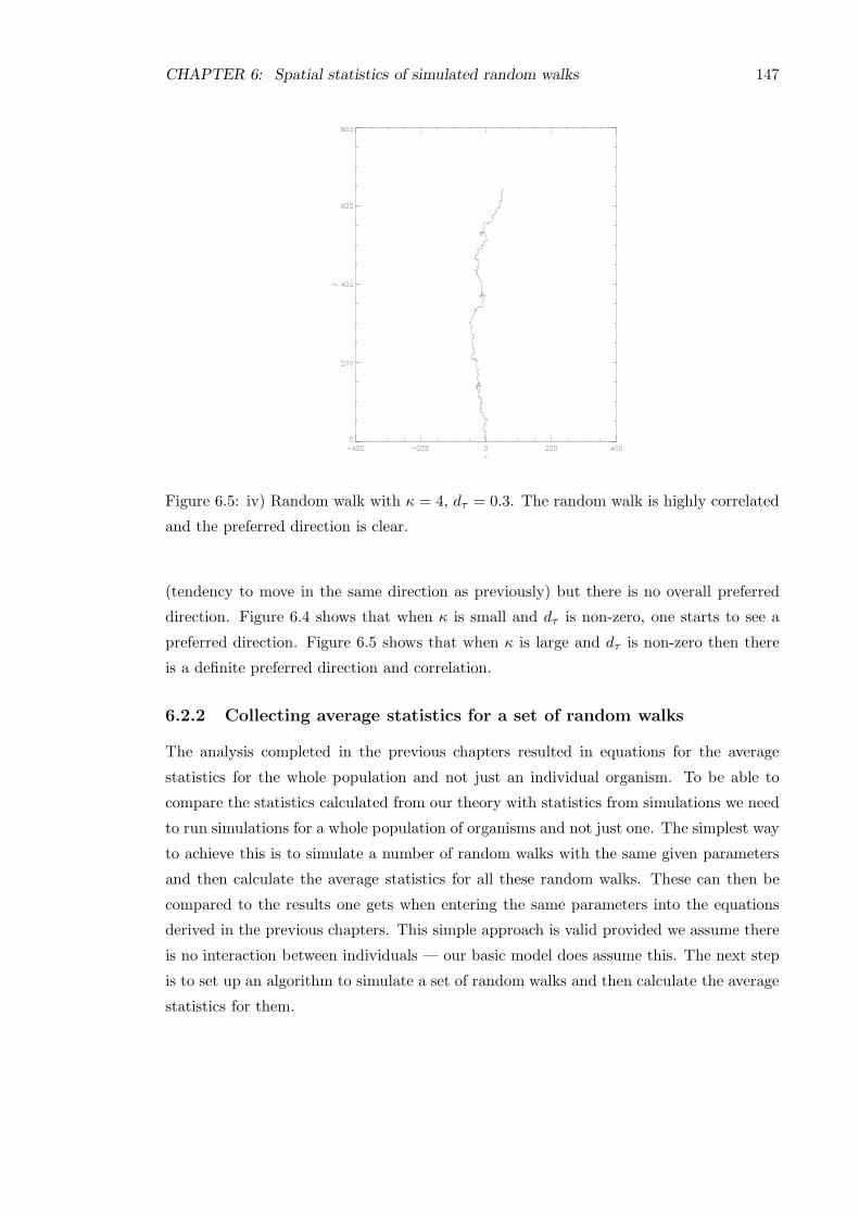
CHAPTER 6: Spatial statistics of simulated random walks 147
Figure 6.5: iv) Random walk with κ = 4, dτ = 0.3. The random walk is highly correlated
and the preferred direction is clear.
(tendency to move in the same direction as previously) but there is no overall preferred
direction. Figure 6.4 shows that when κ is small and dτ is non-zero, one starts to see a
preferred direction. Figure 6.5 shows that when κ is large and dτ is non-zero then there
is a definite preferred direction and correlation.
6.2.2 Collecting average statistics for a set of random walks
The analysis completed in the previous chapters resulted in equations for the average
statistics for the whole population and not just an individual organism. To be able to
compare the statistics calculated from our theory with statistics from simulations we need
to run simulations for a whole population of organisms and not just one. The simplest way
to achieve this is to simulate a number of random walks with the same given parameters
and then calculate the average statistics for all these random walks. These can then be
compared to the results one gets when entering the same parameters into the equations
derived in the previous chapters. This simple approach is valid provided we assume there
is no interaction between individuals — our basic model does assume this. The next step
is to set up an algorithm to simulate a set of random walks and then calculate the average
statistics for them.

CHAPTER 6: Spatial statistics of simulated random walks 148
1) Enter parameter values and initialconditions.
2) Simulate an individual random walkwith given parameters.
4) Stop after required number of randomwalks (ie. required population size).
3) Send position data to a results file.
5) Apply required sampling length toresults file.
6) Calculate average statistics for eachtime step from data.
7) Calculate confidence intervals forthe average staistics at each time step.
8) Calculate average statistics for eachtime step from equations.
9) Stop after required number of timesteps.
Figure 6.6: Algorithm used to calculate average statistics for a set of random walks.

CHAPTER 6: Spatial statistics of simulated random walks 149
6.2.2.1 Algorithm to simulate a population of random walkers
Step 1
As described in the previous section, certain parameters and initial conditions need to be
entered into the algorithm. The parameters are the same as those needed in simulating
an individual random walk. One also needs to enter the population size (number of
random walks to be simulated). All the random walks use the same parameters and initial
conditions. We assume that the population all start at the same point, (x0, y0) = (0, 0),
and initial orientations θ0 are chosen randomly from a uniform distribution on a unit circle
(so for a large population we would expect E(cos θ0) ≈ 0).
Steps 2 and 3
This part of the algorithm is simply the algorithm for an individual random walk repeated
as many times as necessary. This produces a data file with a set of ‘runs’ each of the same
length. Each ‘run’ consists of the (x, y) position at each unit time step.
Step 4
The algorithm includes a counter that counts the number of ‘runs’ completed so far. When
this reaches the required population size the algorithm moves on to the next step.
Step 5
The data file consists of a set of ‘runs’ each of which consists of a list of coordinates at each
time step. It is possible to produce a second data file from this first file where one looks
at the coordinates at every second time step (or third, or fourth etc). This is effectively
changing the sampling length used. This will be investigated further in Chapter 7 when
looking at angular statistics and for the results presented in this chapter the time step
remains unchanged and the data file is thus also unchanged.
Steps 6, 7 and 8
The algorithm now looks through the data file taking the coordinates for the first time step
in each ‘run’ and calculating average statistics from them. The algorithm also calculates
the values predicted by the equations derived in the previous chapter for the average
statistics. This part of the algorithm uses a program taken from Numerical Recipes (Press
et al., 1992) to calculate Bessel functions (BESSI). These steps form a loop in the program,
the algorithm moving onto the next time step in each run after every loop.

CHAPTER 6: Spatial statistics of simulated random walks 150
Step 9
A counter is again used to track where the algorithm is in the data file. When the end of
the data file is reached the algorithm stops and the results for each time step are presented
in a new data file.
6.3 Simulations to validate theoretical results
In the following systematic study a number of simulations were carried out using the
algorithm in Figure 6.6. The results of the simulation and the expected value given by our
theory are then compared and displayed as a set of plots. The turning rate and speed are
both fixed for all the simulations (λ = 1 and s = 1), this is effectively non-dimensionalising
with respect to time as discussed in Section 4.9.2. The only parameters that are changed
between each simulation run are κ and dτ . Each simulation run used a population of 1000
walkers (n = 1000) and produced statistics from t = 0 to t = 100.
All the subsequent plots are samples of the behaviour of the population. Each simulation
run looks at the movement of 1000 walkers, and by nature each individual run includes
a lot of ‘random noise.’ For this reason no two simulation runs will be exactly the same
and will give slightly different plots each time. What we have included is typical plots of
the average behaviour. When looking at a particular statistic, completely new runs were
simulated. This means for example, that the simulation run to calculate H(t) with κ = 2
and dτ = 0.1 is a different simulation run to the run to calculate σ2(t) with κ = 2 and
dτ = 0.1.
6.3.1 Mean position — H(t)
The mean position is only non-zero in the preferred direction (which we assume to be the
y-direction in our model, so in the notation of the previous chapters x1 = y and x2 = x).
The expected mean position in the non-preferred direction (x2 = x) is always 0. Hence,
in the following studies we look at the mean of the position in the y-direction (i.e. we
use Hy(t)). As there is a relatively large amount of random noise in the mean position
for smaller values of the parameters, even with n = 1000, the comparison between theory
and simulation has been done by comparing the theoretical value with a 95% confidence
interval calculated from the sample mean and variance.
6.3.1.1 Confidence intervals for the population mean
Clarke & Cooke (1992) give the following definitions for the confidence interval of a pop-
ulation mean. In sampling from a normal distribution with known variance σ2 and whose
mean takes some unknown value µ, the sample mean x has a N(µ, σ2/n) distribution.
Also, Z =√n(x− µ)/σ has a N(0, 1) distribution. Using a standard table of the normal

CHAPTER 6: Spatial statistics of simulated random walks 151
distribution, we can say that
Pr(−1.96 ≤ x− µ
σ/√n≤ +1.96) = 0.95.
This statement is equivalent to
Pr(x− 1.96σ/√n ≤ µ ≤ x+ 1.96σ/
√n) = 0.95. (6.1)
We call the interval in the brackets a 95% confidence interval for µ.
Using the Central Limit Theorem, in general the mean of a non-normal distribution will
tend to be normally distributed as the sample size increases. Let us now suppose that a
large sample is available, of n observations from a non-normal distribution. The statement
in (6.1) is now true with probability approximately 0.95, rather than exactly.
If we do not know the population variance σ2, then we must use the estimated standard
deviation s instead of σ. When the sample size is small the ratio
x− µ
s/√n
has a t-distribution, with (n − 1) degrees of freedom, rather than a normal distribution.
The appropriate 95% confidence interval is
x− s√nt(n−1,0.05) ≤ µ ≤ x+
s√nt(n−1,0.05).
As the sample size n increases, the t-distribution becomes closer to the normal distribution.
In fact, t(120,0.05) = 1.98 and as n increases t(n−1,0.05) approaches the value 1.96. In our
simulations we will be dealing with sample sizes of n = 1000 so an appropriate 95 %
confidence interval for the population mean in our simulations is
x− 1.96s√n≤ µ ≤ x+ 1.96
s√n
(6.2)
To calculate the confidence interval for Hy(t), we must use the sample variance in the
y-direction, σ2y(t), not the sample value of the total variance σ2(t).
6.3.1.2 Results for the sinusoidal reorientation model
Plots comparing the mean position Hy(t) from our theoretical equation with sinusoidal
reorientation (4.93) to simulated random walks are shown in Figures 6.7 — 6.9. When
dτ = 0 there is no bias and no overall drift so that Hy(t) = 0, and plots are omitted.
6.3.1.3 Comments on the sinusoidal reorientation model
The plots displayed in Figures 6.7-6.9 show for various values of κ and dτ , the theoretical
expected value for the mean y-position calculated from our equation for Hy(t) with a
sinusoidal reorientation model (4.93), and a 95% confidence interval calculated from the
simulation mean and variance.

CHAPTER 6: Spatial statistics of simulated random walks 152
(a) κ = 0.1, dτ = 0.1. (b) κ = 0.5, dτ = 0.1.
(c) κ = 1, dτ = 0.1. (d) κ = 2, dτ = 0.1.
(e) κ = 4, dτ = 0.1. (f) κ = 8, dτ = 0.1.
Figure 6.7: Plots showing theoretical Hy(t) (—), and 95% confidence interval from sim-
ulated (· · ·), against time for sinusoidal reorientation with dτ = 0.1. (The scale used for
each plot is different.)

CHAPTER 6: Spatial statistics of simulated random walks 153
(a) κ = 0.1, dτ = 0.2. (b) κ = 0.5, dτ = 0.2.
(c) κ = 1, dτ = 0.2. (d) κ = 2, dτ = 0.2.
(e) κ = 4, dτ = 0.2. (f) κ = 8, dτ = 0.2.
Figure 6.8: Plots showing theoretical Hy(t) (—), and 95% confidence interval from sim-
ulated (· · ·), against time for sinusoidal reorientation with dτ = 0.2. (The scale used for
each plot is different.)

CHAPTER 6: Spatial statistics of simulated random walks 154
(a) κ = 0.1, dτ = 0.3. (b) κ = 0.5, dτ = 0.3.
(c) κ = 1, dτ = 0.3. (d) κ = 2, dτ = 0.3.
(e) κ = 4, dτ = 0.3. (f) κ = 8, dτ = 0.3.
Figure 6.9: Plots showing theoretical Hy(t) (—), and 95% confidence interval from sim-
ulated (· · ·), against time for sinusoidal reorientation with dτ = 0.3. (The scale used for
each plot is different.)

CHAPTER 6: Spatial statistics of simulated random walks 155
Simulations with 0.1 ≤ dτ ≤ 0.2.
When dτ 6= 0 we have a bias towards the y-direction and there is an overall drift in this
direction. Looking at the plots shown in Figures 6.7 — 6.9, our theoretical solutions are a
good fit to the simulations for all these values of the parameters. There is a larger absolute
velocity as κ and dτ increase.
Simulations with dτ = 0.3.
When dτ = 0.3 we need to consider the limits imposed on κ and dτ as discussed earlier
(see Section 4.9.3). Looking at the plots shown in Figure 6.9, our theoretical solutions
are a good fit to the simulation results up to κ = 4, but when κ = 8 our theoretical
solution appears to overestimate the simulation results slightly. As discussed earlier when
calculating limits on the parameters (Section 4.9.3), this is only a very small relative error
when looking at just the average position but when calculating σ2y(t) this error can result
in nonsensical solutions.
Our theoretical solution for the mean y-position, Hy(t), with sinusoidal reorientation from
(4.93), appears to be a good fit to results from simulations, except for the extreme values
of the parameters κ and dτ . When one approaches the limiting values of these parameters
then our model starts to break down and produce an overestimating error that, although
relatively small, can produce nonsensical results when looking at σ2y(t) as discussed in
Section 4.9.3. This is due to the fact that we assumed dτ ≪ 1 and approximated higher
order moments in our derivation of the solution equations. As dτ and κ get larger then
these assumptions become less valid.
6.3.1.4 Results for the linear reorientation model
Plots comparing the mean position Hy(t) for our theoretical equation with linear reorien-
tation (5.93) to simulated random walks are shown in Figures 6.10 — 6.12. When dτ = 0
there is no bias and no overall drift so that Hy(t) = 0, and plots are omitted.
6.3.1.5 Comments on the linear reorientation model
The plots in Figures 6.10-6.12 show for various values of κ and dτ , the theoretical expected
value for the mean y-position calculated from our equation for Hy(t) with a linear reori-
entation model, and a 95% confidence interval calculated from the simulation mean and
variance.
We have similar results to the sinusoidal model although it should be noted that the linear
model has a larger absolute velocity than the sinusoidal model, as expected.

CHAPTER 6: Spatial statistics of simulated random walks 156
(a) κ = 0.1, dτ = 0.1. (b) κ = 0.5, dτ = 0.1.
(c) κ = 1, dτ = 0.1. (d) κ = 2, dτ = 0.1.
(e) κ = 4, dτ = 0.1. (f) κ = 8, dτ = 0.1.
Figure 6.10: Plots showing theoretical Hy(t) (—), and 95% confidence interval from sim-
ulated (· · ·), against time for linear reorientation with dτ = 0.1. (The scale used for each
plot is different.)

CHAPTER 6: Spatial statistics of simulated random walks 157
(a) κ = 0.1, dτ = 0.2. (b) κ = 0.5, dτ = 0.2.
(c) κ = 1, dτ = 0.2. (d) κ = 2, dτ = 0.2.
(e) κ = 4, dτ = 0.2. (f) κ = 8, dτ = 0.2.
Figure 6.11: Plots showing theoretical Hy(t) (—), and 95% confidence interval from sim-
ulated (· · ·), against time for linear reorientation with dτ = 0.2. (The scale used for each
plot is different.)

CHAPTER 6: Spatial statistics of simulated random walks 158
(a) κ = 0.1, dτ = 0.3. (b) κ = 0.5, dτ = 0.3.
(c) κ = 1, dτ = 0.3. (d) κ = 2, dτ = 0.3.
(e) κ = 4, dτ = 0.3. (f) κ = 8, dτ = 0.3.
Figure 6.12: Plots showing theoretical Hy(t) (—), and 95% confidence interval from sim-
ulated (· · ·), against time for linear reorientation with dτ = 0.3. (The scale used for each
plot is different.)

CHAPTER 6: Spatial statistics of simulated random walks 159
Simulations with 0 < dτ ≤ 0.3.
When dτ 6= 0 we have a bias towards the y-direction and there is an overall drift in this
direction. Looking at the plots shown in Figures 6.10 — 6.12, our theoretical solutions are
a good fit to the simulations for these values of the parameters. There is a larger absolute
velocity as κ increases.
It is not clear that our theoretical solution starts to break down and overestimate the simu-
lated results as in the sinusoidal model but as discussed previously, even very small relative
errors can produce nonsensical results when calculating theoretical values for σ2x1(t).
Our theoretical model for Hy(t), the mean y-position, for linear reorientation, appears
to be a good fit to results from simulations for all values of the parameters used. This
suggests that, even though we had to fit simple functions to the intractable integrals during
the derivation of the linear solution equations, the linear solution equations for Hy(t) are
possibly a better fit than the sinusoidal solution equations for the more extreme parameter
values.
6.3.2 Average velocity — V(t)
6.3.2.1 Absolute and instantaneous velocity
The equations derived in the previous chapters for V(t), give the instantaneous velocity
at a particular point in time. This is the average direction that the population is moving
in at that instant. Due to the random nature of our model and the simulations, this
instantaneous velocity will include an amount of random noise — even if the population is
moving steadily in the average direction there can still be large random fluctuations in the
instantaneous velocity at any time step. It is more useful to look at the absolute velocity,
H(t)/t. The absolute velocity will have less random fluctuations as t increases, and the
limiting values of both Vy(t) and Hy(t)/t are the same. We have compared theoretical
results to simulations for dτ = 0.1 and dτ = 0.3 only, to illustrate some of the points made
in the previous section.
6.3.2.2 Results for sinusoidal reorientation model
Plots comparing the absolute velocity Hy(t)/t for our theoretical model with sinusoidal
reorientation to simulated random walks are shown in Figure 6.13 and Figure 6.14.
6.3.2.3 Comments on the sinusoidal reorientation model
The plots shown in Figures 6.13 and 6.14 confirm the results that we found for the average
position Hy(t). Allowing for the random noise in the simulations, the only plot that
seems to show a large error between theory and simulation is the plot with κ = 8 and

CHAPTER 6: Spatial statistics of simulated random walks 160
(a) κ = 0.1, dτ = 0.1. (b) κ = 0.5, dτ = 0.1.
(c) κ = 1, dτ = 0.1. (d) κ = 2, dτ = 0.1.
(e) κ = 4, dτ = 0.1. (f) κ = 8, dτ = 0.1.
Figure 6.13: Plots showing theoretical (—), and simulated (· · ·), absolute velocity
(Hy(t)/t) in the y-direction against time for sinusoidal reorientation with dτ = 0.1. (The
scale used for each plot is different.)

CHAPTER 6: Spatial statistics of simulated random walks 161
(a) κ = 0.1, dτ = 0.3. (b) κ = 0.5, dτ = 0.3.
(c) κ = 1, dτ = 0.3. (d) κ = 2, dτ = 0.1.
(e) κ = 4, dτ = 0.3. (f) κ = 8, dτ = 0.3.
Figure 6.14: Plots showing theoretical (—), and simulated (· · ·) absolute velocity (Hy(t)/t)
in the y-direction against time for sinusoidal reorientation with dτ = 0.3. (The scale used
for each plot is different.)

CHAPTER 6: Spatial statistics of simulated random walks 162
dτ = 0.3. In this case the theoretical solution is bigger than the solution obtained from
simulations. This fits with the conclusion made earlier that when κ and dτ are both large,
our theoretical solutions break down and overestimate the average position and hence the
absolute velocity as well.
In general, the simulation and theoretical solutions are very similar, although there is a lot
of random noise when t is close to zero — this is because we have a random spread of initial
directions. As time increases, the simulation solution tends to a constant limiting value
that is very close to that predicted by our theory (except for the extreme case discussed
above).
6.3.2.4 Results for linear reorientation model
Plots comparing the absolute velocity Hy(t)/t for our theoretical model with linear reori-
entation to simulated random walks are shown in Figure 6.15 and Figure 6.16.
6.3.2.5 Comments on the linear reorientation model
The plots shown in Figures 6.15 and 6.16 confirm the results that we found for the average
position Hy(t). Allowing for the random noise in the simulations at smaller parameter
values and small t, all the theoretical and simulated plots show a good match.
6.3.3 Measure of spread about the origin — D2(t)
Our theory predicts spread about the origin in both the x and y-directions, D2(t) being the
sum of the spread in each of the directions. As the simulations do not seem to introduce
significant random noise in the average spread about the origin, D2(t), the comparison
between theory and simulation has been made by just comparing the theoretical values
with the simulation values.
As the average position becomes further and further away from the origin (as we expect in
a biased random walk), then D2(t) becomes less useful as a statistic. In the extreme cases
when one is almost moving linearly then the statistic D2(t) ∼ Hy(t)2. The spread about
the mean position σ2(t) is a more useful statistic to look at when dealing with a biased
random walk. When dτ = 0, there is no bias and the spread about the mean position is
the same as the spread about the origin, D2(t) = σ2(t) — this case has been included in
the section looking at σ2(t).
6.3.3.1 Results for sinusoidal reorientation model
Plots comparing the mean squared displacement D2(t) for our theoretical equation with
sinusoidal reorientation to simulated random walks are shown in Figure 6.17 and Figure
6.18.

CHAPTER 6: Spatial statistics of simulated random walks 163
(a) κ = 0.1, dτ = 0.1. (b) κ = 0.5, dτ = 0.1.
(c) κ = 1, dτ = 0.1. (d) κ = 2, dτ = 0.1.
(e) κ = 4, dτ = 0.1. (f) κ = 8, dτ = 0.1.
Figure 6.15: Plots showing theoretical (—), and simulated (· · ·), absolute velocity
(Hy(t)/t) in the y-direction against time for linear reorientation with dτ = 0.1. (The
scale used for each plot is different.)

CHAPTER 6: Spatial statistics of simulated random walks 164
(a) κ = 0.1, dτ = 0.3. (b) κ = 0.5, dτ = 0.3.
(c) κ = 1, dτ = 0.3. (d) κ = 2, dτ = 0.3.
(e) κ = 4, dτ = 0.3. (f) κ = 8, dτ = 0.3.
Figure 6.16: Plots showing theoretical (—), and simulated (· · ·), absolute velocity
(Hy(t)/t) in the y-direction against time for linear reorientation with dτ = 0.3. (The
scale used for each plot is different.)

CHAPTER 6: Spatial statistics of simulated random walks 165
(a) κ = 0.1, dτ = 0.1. (b) κ = 0.5, dτ = 0.1.
(c) κ = 1, dτ = 0.1. (d) κ = 2, dτ = 0.1.
(e) κ = 4, dτ = 0.1. (f) κ = 8, dτ = 0.1.
Figure 6.17: Plots showing theoretical (—), and simulated (· · ·), D2(t) against time for
sinusoidal reorientation with dτ = 0.1. (The scale used for each plot is different.)
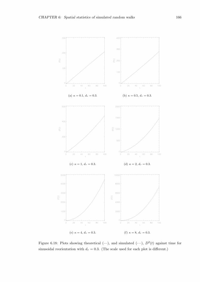
CHAPTER 6: Spatial statistics of simulated random walks 166
(a) κ = 0.1, dτ = 0.3. (b) κ = 0.5, dτ = 0.3.
(c) κ = 1, dτ = 0.3. (d) κ = 2, dτ = 0.3.
(e) κ = 4, dτ = 0.3. (f) κ = 8, dτ = 0.3.
Figure 6.18: Plots showing theoretical (—), and simulated (· · ·), D2(t) against time for
sinusoidal reorientation with dτ = 0.3. (The scale used for each plot is different.)
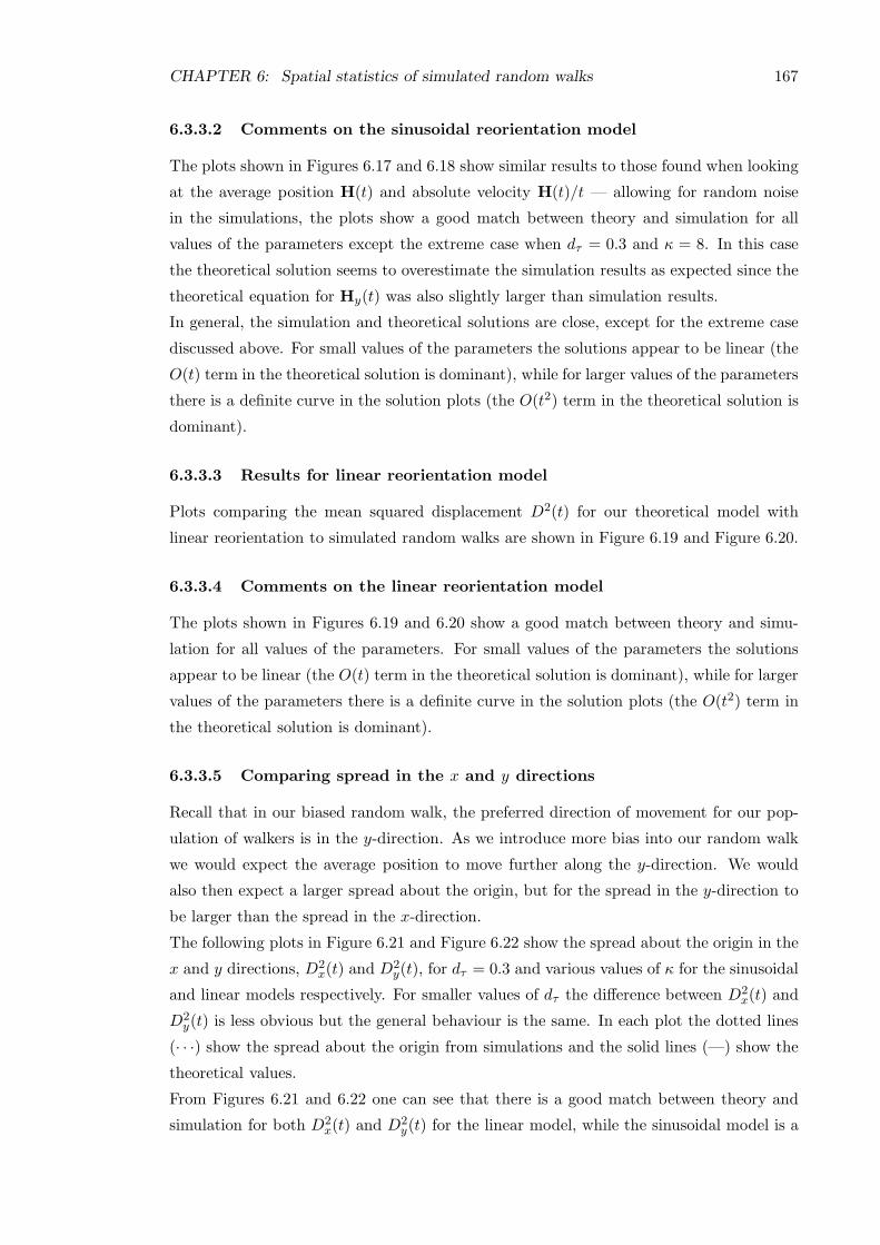
CHAPTER 6: Spatial statistics of simulated random walks 167
6.3.3.2 Comments on the sinusoidal reorientation model
The plots shown in Figures 6.17 and 6.18 show similar results to those found when looking
at the average position H(t) and absolute velocity H(t)/t — allowing for random noise
in the simulations, the plots show a good match between theory and simulation for all
values of the parameters except the extreme case when dτ = 0.3 and κ = 8. In this case
the theoretical solution seems to overestimate the simulation results as expected since the
theoretical equation for Hy(t) was also slightly larger than simulation results.
In general, the simulation and theoretical solutions are close, except for the extreme case
discussed above. For small values of the parameters the solutions appear to be linear (the
O(t) term in the theoretical solution is dominant), while for larger values of the parameters
there is a definite curve in the solution plots (the O(t2) term in the theoretical solution is
dominant).
6.3.3.3 Results for linear reorientation model
Plots comparing the mean squared displacement D2(t) for our theoretical model with
linear reorientation to simulated random walks are shown in Figure 6.19 and Figure 6.20.
6.3.3.4 Comments on the linear reorientation model
The plots shown in Figures 6.19 and 6.20 show a good match between theory and simu-
lation for all values of the parameters. For small values of the parameters the solutions
appear to be linear (the O(t) term in the theoretical solution is dominant), while for larger
values of the parameters there is a definite curve in the solution plots (the O(t2) term in
the theoretical solution is dominant).
6.3.3.5 Comparing spread in the x and y directions
Recall that in our biased random walk, the preferred direction of movement for our pop-
ulation of walkers is in the y-direction. As we introduce more bias into our random walk
we would expect the average position to move further along the y-direction. We would
also then expect a larger spread about the origin, but for the spread in the y-direction to
be larger than the spread in the x-direction.
The following plots in Figure 6.21 and Figure 6.22 show the spread about the origin in the
x and y directions, D2x(t) and D2
y(t), for dτ = 0.3 and various values of κ for the sinusoidal
and linear models respectively. For smaller values of dτ the difference between D2x(t) and
D2y(t) is less obvious but the general behaviour is the same. In each plot the dotted lines
(· · ·) show the spread about the origin from simulations and the solid lines (—) show the
theoretical values.
From Figures 6.21 and 6.22 one can see that there is a good match between theory and
simulation for both D2x(t) and D2
y(t) for the linear model, while the sinusoidal model is a

CHAPTER 6: Spatial statistics of simulated random walks 168
(a) κ = 0.1, dτ = 0.1. (b) κ = 0.5, dτ = 0.1.
(c) κ = 1, dτ = 0.1. (d) κ = 2, dτ = 0.1.
(e) κ = 4, dτ = 0.1. (f) κ = 8, dτ = 0.1.
Figure 6.19: Plots showing theoretical (—), and simulated (· · ·), D2(t) against time for
linear reorientation with dτ = 0.1. (The scale used for each plot is different.)

CHAPTER 6: Spatial statistics of simulated random walks 169
(a) κ = 0.1, dτ = 0.3. (b) κ = 0.5, dτ = 0.3.
(c) κ = 1, dτ = 0.3. (d) κ = 2, dτ = 0.3.
(e) κ = 4, dτ = 0.3. (f) κ = 8, dτ = 0.3.
Figure 6.20: Plots showing theoretical (—), and simulated (· · ·), D2(t) against time for
linear reorientation with dτ = 0.3. (The scale used for each plot is different.)

CHAPTER 6: Spatial statistics of simulated random walks 170
(a) D2
x(t) with κ = 0.1, dτ =
0.3.
(b) D2
y(t) with κ = 0.1, dτ =
0.3.
(c) D2
x(t) with κ = 2.0, dτ =
0.3.
(d) D2
y(t) with κ = 2.0, dτ =
0.3.
(e) D2
x(t) with κ = 8.0, dτ =
0.3.
(f) D2
y(t) with κ = 8.0, dτ =
0.3.
Figure 6.21: Plots showing D2x(t) and D2
y(t) against time for sinusoidal reorientation with
various values of the parameters. (The scale used for each plot is different.)

CHAPTER 6: Spatial statistics of simulated random walks 171
(a) D2
x(t) with κ = 0.1, dτ =
0.3.
(b) D2
y(t) with κ = 0.1, dτ =
0.3.
(c) D2
x(t) with κ = 2.0, dτ =
0.3.
(d) D2
y(t) with κ = 2.0, dτ =
0.3.
(e) D2
x(t) with κ = 8.0, dτ =
0.3.
(f) D2
y(t) with κ = 8.0, dτ =
0.3.
Figure 6.22: Plots showing D2x(t) and D2
y(t) against time for linear reorientation with
various values of the parameters. (The scale used for each plot is different.)

CHAPTER 6: Spatial statistics of simulated random walks 172
good match up to κ = 8 when we know our theoretical results are unreliable. It is clear
that as κ increases the difference between D2x(t) and D2
y(t) becomes greater. The plots
of D2x(t) are linear in t while those for D2
y(t) become more like t2 as κ increases. When
κ = 8, the sinusoidal model overestimates the true value of D2y(t), but this is expected
as our equation for Hy(t) also overestimates simulation results when the parameters are
this large. When κ = 8, the solution for the sinusoidal case for D2x(t) underestimates the
simulation results. In all cases, the linear model gives significantly larger values for D2y(t),
while D2x(t) is similar for both models.
6.3.4 Measure of spread about the mean position — σ2(t)
As was the case with D2(t), our theory predicts spread about the mean position in both
the x and y-directions, σ2(t) being the sum of the spread in each of the directions. As
the simulations do not seem to introduce significant random noise in the average spread
about the mean position, σ2(t), the comparison between theory and simulation has been
done by just comparing the theoretical values with the simulation values.
6.3.4.1 Results for sinusoidal reorientation model
Plots comparing the spread about the mean position σ2(t) for our theoretical model with
sinusoidal reorientation to simulated random walks are shown in Figures 6.23 — 6.26.
6.3.4.2 Comments on the sinusoidal reorientation model
The plots displayed in Figures 6.23 - 6.26 show, for various values of κ and dτ , the theo-
retical expected value for the average spread about the mean position calculated from our
equation for σ2(t) with sinusoidal reorientation. Looking at the solution plots it is clear
that, allowing for the random nature of the simulations, the theoretical solution equation
fits the simulations almost exactly for all smaller values of the parameters, and only breaks
down and underestimates the actual spread when dτ = 0.2 and κ = 8, or dτ = 0.3 and
κ ≥ 4. This is unsurprising as we know that our equations for the spread are likely to be
unreliable at these extreme values of the parameters.
In general, as we increase κ the spread σ2(t) increases until we reach the extreme values of
the parameters when the spread starts to decrease. This is because as we increase the size
of the parameters we are finding that the walkers are tending to all move in the preferred
direction. If we kept increasing the parameters, eventually we would expect motion in
a straight line directly in the y-direction, and the total spread about the mean position
would be close to zero.

CHAPTER 6: Spatial statistics of simulated random walks 173
(a) κ = 0.1, dτ = 0. (b) κ = 0.5, dτ = 0.
(c) κ = 1, dτ = 0. (d) κ = 2, dτ = 0.
(e) κ = 4, dτ = 0. (f) κ = 8, dτ = 0.
Figure 6.23: Plots showing theoretical (—), and simulated (· · ·), σ2(t) against time for
sinusoidal reorientation with dτ = 0. (The scale used for each plot is different.)

CHAPTER 6: Spatial statistics of simulated random walks 174
(a) κ = 0.1, dτ = 0.1. (b) κ = 0.5, dτ = 0.1.
(c) κ = 1, dτ = 0.1. (d) κ = 2, dτ = 0.1.
(e) κ = 4, dτ = 0.1. (f) κ = 8, dτ = 0.1.
Figure 6.24: Plots showing theoretical (—), and simulated (· · ·), σ2(t) against time for
sinusoidal reorientation with dτ = 0.1. (The scale used for each plot is different.)

CHAPTER 6: Spatial statistics of simulated random walks 175
(a) κ = 0.1, dτ = 0.2. (b) κ = 0.5, dτ = 0.2.
(c) κ = 1, dτ = 0.2. (d) κ = 2, dτ = 0.2.
(e) κ = 4, dτ = 0.2. (f) κ = 8, dτ = 0.2.
Figure 6.25: Plots showing theoretical (—), and simulated (· · ·), σ2(t) against time for
sinusoidal reorientation with dτ = 0.2. (The scale used for each plot is different.)

CHAPTER 6: Spatial statistics of simulated random walks 176
(a) κ = 0.1, dτ = 0.3. (b) κ = 0.5, dτ = 0.3.
(c) κ = 1, dτ = 0.3. (d) κ = 2, dτ = 0.3.
(e) κ = 4, dτ = 0.3. (f) κ = 8, dτ = 0.3.
Figure 6.26: Plots showing theoretical (—), and simulated (· · ·), σ2(t) against time for
sinusoidal reorientation with dτ = 0.3. (The scale used for each plot is different.)

CHAPTER 6: Spatial statistics of simulated random walks 177
6.3.4.3 Results for linear reorientation model
Plots comparing the spread about the mean position σ2(t) for our theoretical model with
linear reorientation to simulated random walks are shown in Figures 6.27 — 6.29.
When dτ = 0, the motion is the same for both the sinusoidal and linear models — both
will have zero response to the bias. Thus plots for linear reorientation with dτ = 0 are
omitted as the behaviour is the same as that shown in Figure 6.23.
6.3.4.4 Comments on the linear reorientation model
The plots displayed in Figures 6.23 — 6.26 show, for various values of κ and dτ , the
theoretical expected value for the average spread about the mean position calculated from
our equation for σ2(t) with linear reorientation. The same conclusions as found with the
sinusoidal model apply — up to the extreme values of the parameters there is an excellent
fit between theoretical and simulation results. At these more extreme parameter values
our theoretical solution underestimates the actual spread.
In general the spread about the mean σ2(t) is less for the linear model than the sinusoidal
model for the same values of the parameters.
6.3.4.5 Comparing spread in the x and y directions
Our theoretical models show a good match to the simulations for the statistic σ2(t) up to
the more extreme values of the parameters. However, as discussed when looking at D2(t),
this statistic is made up of components in the x and y-directions. If dτ 6= 0, these separate
components σ2x(t) and σ2
y(t) are not equal and it is useful to compare the spread about
the mean in each of these directions.
The following plots in Figures 6.30 — 6.33 show the spread about the mean position in the
x and y directions, σ2x(t) and σ2
y(t), for various values of the parameters for the sinusoidal
and linear models respectively. In each plot the dotted lines (· · ·) show the spread about
the mean position from simulations, and the solid lines (—) show the theoretical spread
about the mean position.
From Figures 6.30 — 6.33 one can see that for there is a very good match between theory
and simulation for both σ2x(t) and σ2
y(t) for both the sinusoidal and linear models, except
for the extreme case of dτ = 0.3 and κ = 8.
Sinusoidal model, dτ = 0.3, κ = 8
Looking at Figure 6.31, it is obvious that our model for σ2y(t) breaks down for these
values of the parameters — it is nonsensical to have ‘negative’ spread (see Section 4.9.3).
However, it is an important point to note that the simulated results do show a decrease
in the spread about the mean position. We might expect this spread to tend to zero as
the parameters kept increasing and the motion becomes more like straight line motion. In

CHAPTER 6: Spatial statistics of simulated random walks 178
(a) κ = 0.1, dτ = 0.1. (b) κ = 0.5, dτ = 0.1.
(c) κ = 1, dτ = 0.1. (d) κ = 2, dτ = 0.1.
(e) κ = 4, dτ = 0.1. (f) κ = 8, dτ = 0.1.
Figure 6.27: Plots showing theoretical (—), and simulated (· · ·), σ2(t) against time for
linear reorientation with dτ = 0.1. (The scale used for each plot is different.)

CHAPTER 6: Spatial statistics of simulated random walks 179
(a) κ = 0.1, dτ = 0.2. (b) κ = 0.5, dτ = 0.2.
(c) κ = 1, dτ = 0.2. (d) κ = 2, dτ = 0.2.
(e) κ = 4, dτ = 0.2. (f) κ = 8, dτ = 0.2.
Figure 6.28: Plots showing theoretical (—), and simulated (· · ·), σ2(t) against time for
linear reorientation with dτ = 0.2. (The scale used for each plot is different.)
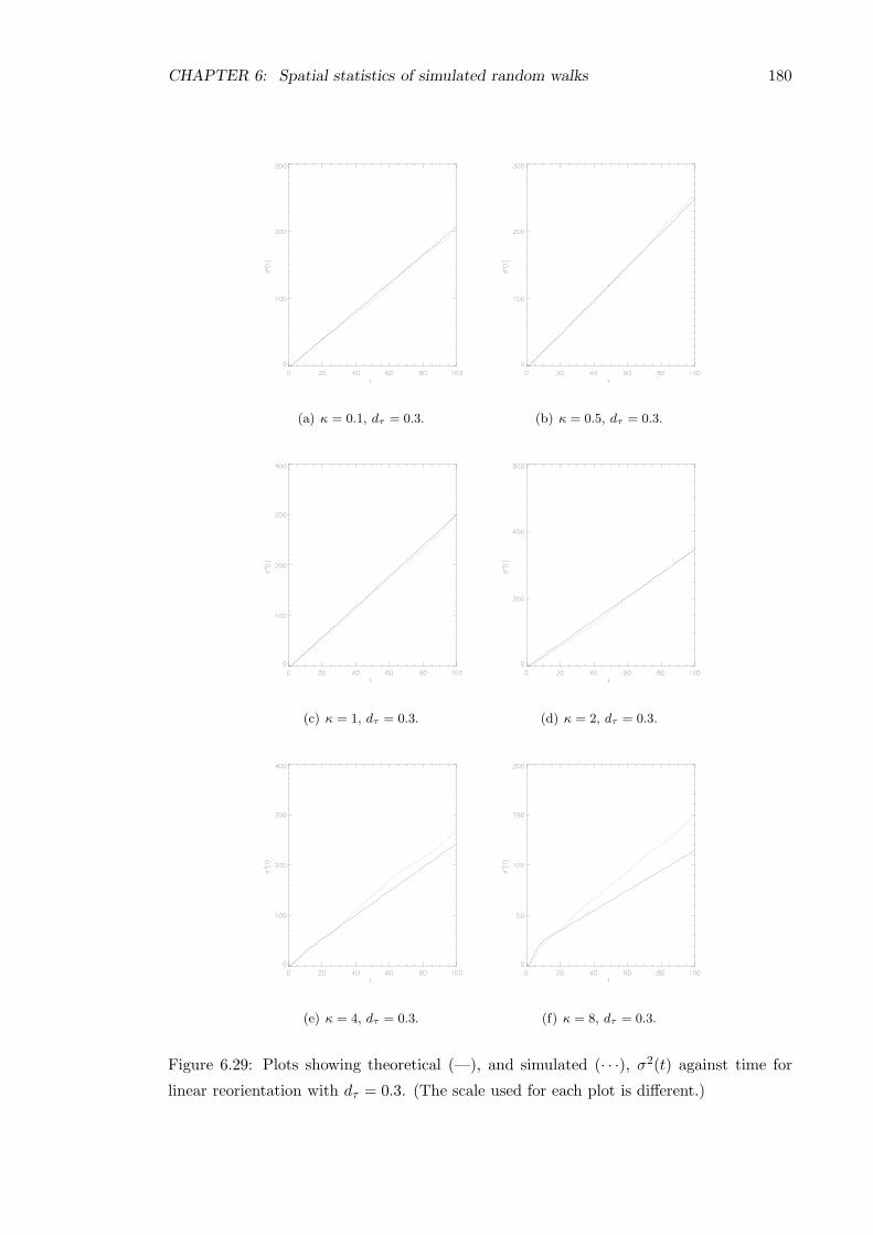
CHAPTER 6: Spatial statistics of simulated random walks 180
(a) κ = 0.1, dτ = 0.3. (b) κ = 0.5, dτ = 0.3.
(c) κ = 1, dτ = 0.3. (d) κ = 2, dτ = 0.3.
(e) κ = 4, dτ = 0.3. (f) κ = 8, dτ = 0.3.
Figure 6.29: Plots showing theoretical (—), and simulated (· · ·), σ2(t) against time for
linear reorientation with dτ = 0.3. (The scale used for each plot is different.)
CHAPTER 6: Spatial statistics of simulated random walks 181
(a) κ = 0.1, dτ = 0.1. (b) κ = 0.1, dτ = 0.3.
(c) κ = 2.0, dτ = 0.1. (d) κ = 2.0, dτ = 0.3.
(e) κ = 8.0, dτ = 0.1. (f) κ = 8.0, dτ = 0.3.
Figure 6.30: Plots showing σ2x(t) against time for sinusoidal reorientation with various
values of the parameters. (The scale used for each plot is different.)

CHAPTER 6: Spatial statistics of simulated random walks 182
(a) κ = 0.1, dτ = 0.1. (b) κ = 0.1, dτ = 0.3.
(c) κ = 2.0, dτ = 0.1. (d) κ = 2.0, dτ = 0.3.
(e) κ = 8.0, dτ = 0.1. (f) κ = 8.0, dτ = 0.3.
Figure 6.31: Plots showing σ2y(t) against time for sinusoidal reorientation with various
values of the parameters. (The scale used for each plot is different.)

CHAPTER 6: Spatial statistics of simulated random walks 183
(a) κ = 0.1, dτ = 0.1. (b) κ = 0.1, dτ = 0.3.
(c) κ = 2.0, dτ = 0.1. (d) κ = 2.0, dτ = 0.3.
(e) κ = 8.0, dτ = 0.1. (f) κ = 8.0, dτ = 0.3.
Figure 6.32: Plots showing σ2x(t) against time for linear reorientation with various values
of the parameters. (The scale used for each plot is different.)

CHAPTER 6: Spatial statistics of simulated random walks 184
(a) κ = 0.1, dτ = 0.1. (b) κ = 0.1, dτ = 0.3.
(c) κ = 2.0, dτ = 0.1. (d) κ = 2.0, dτ = 0.3.
(e) κ = 8.0, dτ = 0.1. (f) κ = 8.0, dτ = 0.3.
Figure 6.33: Plots showing σ2y(t) against time for linear reorientation with various values
of the parameters. (The scale used for each plot is different.)
CHAPTER 6: Spatial statistics of simulated random walks 185
correlated but unbiased random walks the spread always increases as the motion becomes
more like a straight line (Bovet & Benhamou (1988)), and when dτ and κ are small this
is true for our results. However, for a fixed value of dτ , there appears to be a value of κ
after which the spread starts to decrease as the motion becomes more like a straight line.
So even though there is no bias in the x direction, the spread in the direction will start to
decrease. Looking at Figure 6.30(f) it seems that our model for σ2x(t) underestimates the
simulated results in a similar manner to D2x(t) (the statistics are equivalent as Hx(t) = 0).
From the simulation results in Figures 6.30 and 6.31 it is clear that the spread in the
non-preferred direction x is greater than the spread in the preferred direction y for the
extreme values of the parameters discussed above, although both show a decrease in the
spread compared to some smaller values of the parameters.
In all cases the simulated long-time limiting solutions for σ2x(t) and σ2
y(t) appear to be
linear in t, and the spread about the mean position is proportional to the square root of
time — this suggests that the dispersion about the mean position is diffusive.
Linear model, dτ = 0.3, κ = 8
The comments made above for the sinusoidal model apply to the linear model also, al-
though the solution for σ2x(t) is a much better match between theory and simulation. It is
nonsensical to have negative spread and the solution for σ2y(t) breaks down when dτ = 0.3
and κ = 8. In general the spread about the mean in both directions is less for the linear
model than the sinusoidal model for the same values of the parameters.
6.3.4.6 Comparison with an isotropic random walk
From Section 1.1.2.2, we have the expected spread for a completely random (isotropic)
walk
< r2 >=< x2 + y2 >= 4Dt. (6.3)
Recall that when taking the limit of the isotropic random walk we defined δ2/τ ≡ 2D,
thus in a normalized random walk where s = λ = 1, we have D = 12 . From (6.3) we
might expect for a completely random walk using our simulation model that σ2(t) = 2t
and σ2x(t) = σ2
y(t) = t. This is very close to the behaviour observed in the plots displayed
previously for κ = 0.1 (for all values of dτ ), and shows how our model is related to the
standard Brownian diffusion model.
6.4 The effect of the reorientation parameters on fixed time
solutions
In the previous section we have tested the validity of our theoretical solutions for the
sinusoidal and linear reorientation models by comparing to results of simulations. For

CHAPTER 6: Spatial statistics of simulated random walks 186
smaller values of the reorientation parameters κ and dτ there is a very good match between
simulations and theory for all the statistics of interest. In general, it is only the extreme
values of the parameters discussed previously where our theoretical solutions break down.
In this section we complete a more detailed study into the exact effect of the reorientation
parameters on the statistics of interest as we work through the parameter range.
6.4.1 Fixed time spatial distribution
To compare the effect of changing κ and dτ on the solution equations for the spatial
statistics we fix t = 100. Examples to illustrate the spatial distribution at t = 100 for
various parameter values are shown in Figure 6.34. The plots displayed are for simulation
runs with 500 walkers for clarity.
The dotted circle in the plots shows the maximum possible range of movement and hence
with unit speed s = 1, has radius r = 100. The solid circle show a measure of the spread
in each direction. This has been drawn as an ellipse of length rx and height ry with area
A, given by
A = πrxry = πσ2 = π(σ2x + σ2
y), (6.4)
where σx and σy are calculated from the simulation results. The length and width are
related byrxry
=σxσy. (6.5)
Solving (6.4) and (6.5) for rx and ry gives
rx =
√
σxσy +σ3x
σy, (6.6)
and
ry =
√
σxσy +σ3y
σx. (6.7)
Looking at the plots with κ = 8 and dτ = 0.3 in Figure 6.34, one can clearly see the spread
is greater in the x direction than the y direction. Looking at the other plots, one can see
that the spread does increase as κ increases, until one reaches the extreme values of the
parameters.
6.4.2 The effect of changing the reorientation parameters κ and dτ
In this section we carry out a more detailed study of the effect of the parameters dτ and
κ on the solution equations for the spatial statistics.
The following plots all show how the solutions at t = 100 change as the reorientation pa-
rameters vary. The plots of the results from simulations can be compared to our theoretical
solutions for sinusoidal and linear reorientation. The simulation results may contain some
random noise as we are only looking at one time position but the general behaviour should

CHAPTER 6: Spatial statistics of simulated random walks 187
(a) Sinusoidal κ = 0.1, dτ =
0.1.
(b) Linear κ = 0.1, dτ = 0.1.
(c) Sinusoidal κ = 2.0, dτ =
0.2.
(d) Linear κ = 2.0, dτ = 0.2.
(e) Sinusoidal κ = 8.0, dτ =
0.3.
(f) Linear κ = 8.0, dτ = 0.3.
Figure 6.34: Example plots of the population position and spread at t = 100.

CHAPTER 6: Spatial statistics of simulated random walks 188
be clear. All the plots show how the relevant statistic at t = 100 changes as κ increases
from 0 to 8, for 4 values of dτ .
6.4.2.1 Average position H(t)
The plots in Figure 6.35 show how the simulated and theoretical solutions for the average
position in the preferred direction at t = 100, Hy(100), change as the parameter κ increases
from 0 to 8, for dτ = 0, 0.1, 0.2 and 0.3.
(a) Sinusoidal simulation (b) Sinusoidal theory
(c) Linear simulation (d) Linear theory
Figure 6.35: Plots showing Hy(100) against κ for sinusoidal and linear reorientation with
dτ = 0 (—), dτ = 0.1 (· · ·), dτ = 0.2 (−−) and dτ = 0.3 (· − ·).
As observed in the previous section, there is a good match between the simulated and
theoretical solutions displayed in Figure 6.35. The plots all show similar behaviour — for
small values of κ the average position appears to increase linearly as κ increases, with the
greatest rate of increase for the larger values of dτ . Obviously this linear increase cannot

CHAPTER 6: Spatial statistics of simulated random walks 189
continue indefinitely, as in this non-dimensionalised system the maximum displacement at
t = 100 is given by Hy = 100. As κ increases further the rate of increase in Hy(t) slows
and tends asymptotically to the maximum value of 100 as κ→ ∞.
In general, the linear reorientation model gives a larger displacement in the preferred
direction, although at the extreme values of the parameters there is little difference between
the two models.
6.4.2.2 Spread about the origin D2(t)
The plots in Figure 6.36 show how the simulated and theoretical solutions for the spread
about the origin at t = 100, D2(100), change as the parameter κ increases from 0 to 8,
for dτ = 0, 0.1, 0.2 and 0.3. Figure 6.36 shows a good match between the theoretical and
(a) Sinusoidal simulation (b) Sinusoidal theory
(c) Linear simulation (d) Linear theory
Figure 6.36: Plots showing D2(100) against κ for sinusoidal and linear reorientation with
dτ = 0 (—), dτ = 0.1 (· · ·), dτ = 0.2 (−−) and dτ = 0.3 (· − ·).

CHAPTER 6: Spatial statistics of simulated random walks 190
simulated solutions. From the plots the general behaviour as κ increases seems to be a slow
increase in D2(100) at first, then a linear increase, before slowly tending to the asymptotic
limit, which for this system is D2(100) = 10, 000 (corresponding to Hy(100) = 100).
The plots in Figure 6.37 show how the simulated and theoretical solutions for the spread
about the origin in the non-preferred direction at t = 100, D2x(100), change as the param-
eter κ increases from 0 to 8, for dτ = 0, 0.1, 0.2 and 0.3. Figure 6.37 shows a good match
(a) Sinusoidal simulation (b) Sinusoidal theory
(c) Linear simulation (d) Linear theory
Figure 6.37: Plots showing D2x(100) against κ for sinusoidal and linear reorientation with
dτ = 0 (—), dτ = 0.1 (· · ·), dτ = 0.2 (−−) and dτ = 0.3 (· − ·).
between the theoretical and simulated solutions. Recall that the average displacement in
the non-preferred direction is zero, Hx(t) = 0 ∀ t. Thus, the spread about the origin
D2x(t), is the same as the spread about the mean position σ2
x(t). If dτ 6= 0, from Figure
6.37 the general behaviour of D2x(100) as κ increases is a gradual increase before reaching a
maximum value and then decreasing towards zero. For a particular value of κ the spread is

CHAPTER 6: Spatial statistics of simulated random walks 191
greater for the smaller values of dτ . If dτ = 0, the spread increases linearly before tending
towards the asymptotic limit (which in our system is D2x(100) = 5000) as κ → ∞. Bovet
& Benhamou (1988) observed that, in an unbiased random walk the spread will increase
as the correlation (governed by the parameter κ in our model) increases. However, the
presence of bias in a random walk will decrease the spread in the non-preferred direction
in comparison to a completely unbiased random walk. In general, increasing the bias will
decrease the spread in the non-preferred direction for a fixed value of κ. As κ increases
the walkers will move more like a straight line in the preferred direction, leaving less of
the available movement to spread out in the non-preferred direction and this is exactly
the behaviour to be seen in Figure 6.37.
The plots in Figure 6.38 show how the simulated and theoretical solutions for the spread
about the origin in the preferred direction at t = 100, D2y(100), change as the parameter κ
increases from 0 to 8, for dτ = 0, 0.1, 0.2 and 0.3. Figure 6.38 shows a good match between
the theoretical and simulated solutions. The behaviour shown in the plots in Figure 6.38
is almost identical to that shown in Figure 6.36 and the same comments apply. This is
unsurprising since for dτ 6= 0, the spread about the origin in the preferred direction D2y(t)
is always larger than the spread in the non-preferred direction D2x(t), and as κ increases
D2y(t) becomes dominant over D2
x(t), and D2y(t) ∼ D2(t).
6.4.2.3 Spread about the mean position σ2(t)
The plots in Figure 6.39 show how the simulated and theoretical spread about the mean
position at t = 100, σ2(100), change as the parameter κ increases from 0 to 8, for dτ =
0, 0.1, 0.2 and 0.3. In general, Figure 6.39 shows a good match between the theoretical and
simulated solutions. If bias is present then the spread about the mean position σ2(100)
initially increases as κ increases, before reaching a maximum and then starting to decrease
towards zero. For a particular value of κ the spread is less for the larger values of dτ (more
bias). If there is no bias and dτ = 0, then we have a simple correlated random walk and
σ2(100) has the same behaviour as D2(100) with no bias — the spread increases as κ
increases up to the limiting value as described by Bovet & Benhamou (1988). In general,
for the same parameter values the sinusoidal model has more spread about the mean
position than the linear model.
Since the average position in the x direction is zero, we have σ2x(t) = D2
x(t) and the
behaviour of σ2x(t) is given in Figure 6.37. The same comments and conclusions apply.
The plots in Figure 6.40 show how the solutions for the simulated and theoretical spread
about the origin in the preferred direction at t = 100, σ2y(100), change as the parameter
κ increases from 0 to 8, for dτ = 0, 0.1, 0.2 and 0.3. From Figure 6.40 we see that at large
values of κ our solutions break down and give the nonsensical ‘negative spread’ as described
earlier — this is due to the limitations introduced in our modelling process, see Section
4.9.3. However, the qualitative behaviour in the simulated and theoretical solutions is the
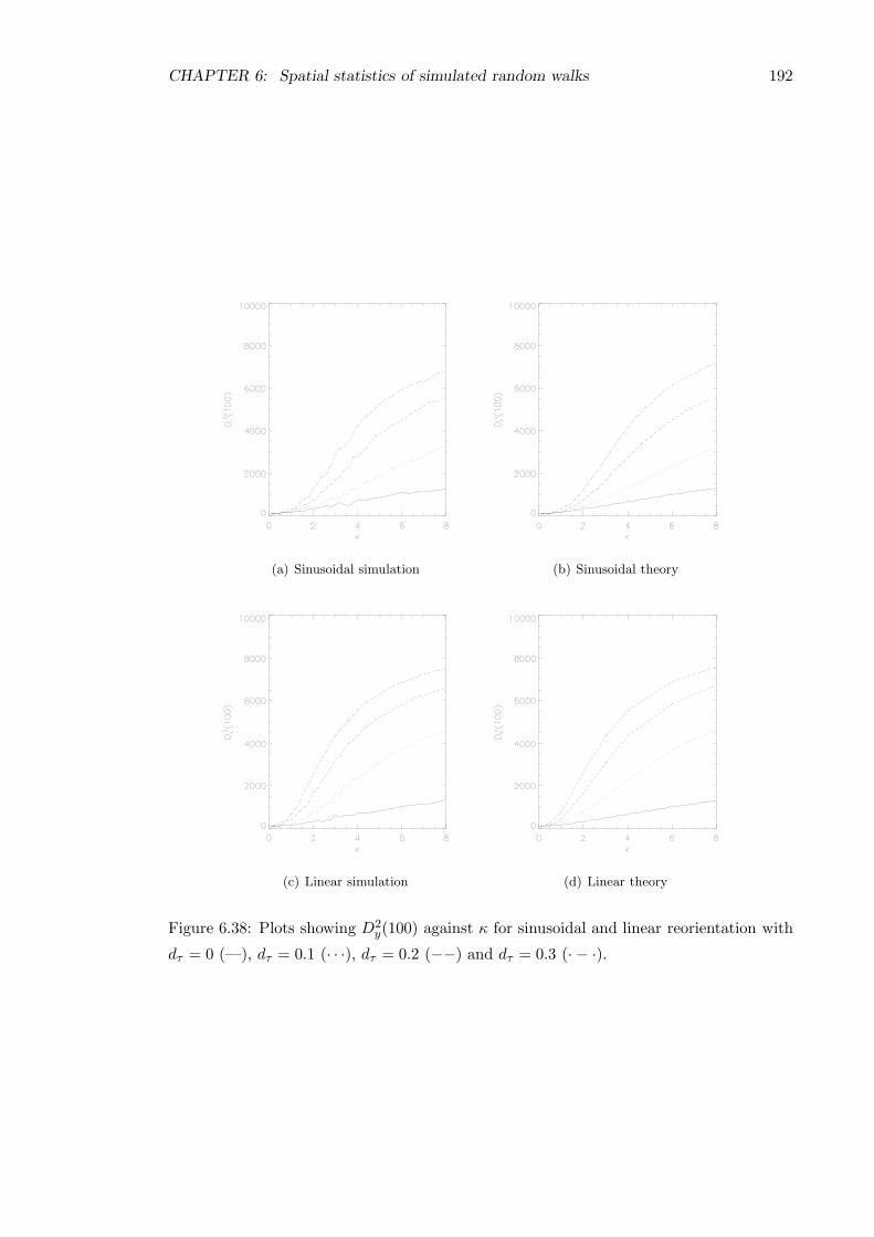
CHAPTER 6: Spatial statistics of simulated random walks 192
(a) Sinusoidal simulation (b) Sinusoidal theory
(c) Linear simulation (d) Linear theory
Figure 6.38: Plots showing D2y(100) against κ for sinusoidal and linear reorientation with
dτ = 0 (—), dτ = 0.1 (· · ·), dτ = 0.2 (−−) and dτ = 0.3 (· − ·).

CHAPTER 6: Spatial statistics of simulated random walks 193
(a) Sinusoidal simulation (b) Sinusoidal theory
(c) Linear simulation (d) Linear theory
Figure 6.39: Plots showing σ2(100) against κ for sinusoidal and linear reorientation with
dτ = 0 (—), dτ = 0.1 (· · ·), dτ = 0.2 (−−) and dτ = 0.3 (· − ·).

CHAPTER 6: Spatial statistics of simulated random walks 194
(a) Sinusoidal simulation (b) Sinusoidal theory
(c) Linear simulation (d) Linear theory
Figure 6.40: Plots showing σ2y(100) against κ for sinusoidal and linear reorientation with
dτ = 0 (—), dτ = 0.1 (· · ·), dτ = 0.2 (−−) and dτ = 0.3 (· − ·).

CHAPTER 6: Spatial statistics of simulated random walks 195
same — for dτ 6= 0 the solutions initially increase, before reaching a maximum and then
decreasing to zero. As κ increases the average motion becomes more like a straight line
in the preferred direction and the spread will decrease to zero corresponding to an exact
straight line when all the movement at each step is in the preferred direction only. As
discussed previously, for a particular value of κ the spread is greater for the sinusoidal
model and also for smaller values of dτ (less bias). For the same parameter values, the
spread about the mean in the preferred direction is less than the spread about the mean
in the non-preferred direction, σ2x(t) > σ2
y(t).
6.5 Simulations with parameters from experimental data
The motivation for including sinusoidal and linear reorientation in our velocity jump pro-
cess model comes from the experimental results of Hill & Hader (1997) as described in
the introductory chapter (Section 1.5). The main results of their experiments are given in
Section 1.5.3. From their data they were unable to determine a value for the angular vari-
ance per unit time σ20 (corresponding to our κ0), and were not certain as to which values
of the sampling time-step τs they should extrapolate back over to estimate the parameter
B−1. Two estimates for the parameter B−1 were given — one by fitting a straight line by
linear regression through the data points for all values of τs, and one by fitting a straight
line by linear regression through the data points for values of τs ≤ 0.4 s only.
The expected long-time angular distributions (1.100) and (1.102) are dependent onB−1/2σ20 ,
so using the observed long-time angular distribution they were able to use (1.100) and
(1.102) with the two given estimates for B−1 to obtain two corresponding estimates for
σ20 . Since both sets of parameter estimates give the same expected long-time angular dis-
tribution they were unable to determine which parameter set was the most realistic. In
this section we show that by observing and analysing the spatial data of experiments as
well as the angular data, it may be possible to overcome the problem described above,
since the two different parameter sets can produce different spatial statistics.
In Hill & Hader’s experiments the mean time step between recorded observations was
τ = 0.08 s. We will use this value as an estimate of the actual time between turns for
our velocity jump model, τ , although it should be noted that this value was obtained as
a consequence of experimental sampling limitations rather than the actual motion of the
algae.
6.5.1 Data set C1 (Sinusoidal model)
From Hill & Hader’s experiments (Section 1.5.3), the data set C1 is obtained from tracking
a population of C. nivalis in a vertical plane guided by negative gravitaxis, the swimming
behaviour being axisymmetric about the vertical axis — this corresponds to our sinusoidal
model. The average speed of movement for this population was found to be v = 55 µms−1.

CHAPTER 6: Spatial statistics of simulated random walks 196
6.5.1.1 Data set C1:a
The results obtained from the data after fitting a straight line by linear regression through
the data points for all values of τs are as follows
B−1 = 0.37,
σ20 = 1.7, which gives κ0 = 0.95.
With these values and τ = 0.08 s we get the following values for the reorientation param-
eters in our sinusoidal velocity jump model (see Section 4.2).
dτ = τB−1 ≈ 0.03,
σ2δ = τσ2
0 ≈ 0.136, which gives κ = 7.89.
Simulations using the sinusoidal reorientation model with these reorientation parameters
and λ = 1/τ = 12.5 s−1 and s = v = 55 µms−1 were completed and the results are
displayed in Figure 6.41.
Figure 6.41(a) shows the spatial distribution at t = 100 (see Section 6.4.1), while Figures
6.41(b) — 6.41(d) show the theoretical (—) and simulated (· · ·) values for the average
position Hy(t), and the spread in the x and y directions, σ2x(t) and σ2
y(t), respectively.
From Figures 6.41(b) — 6.41(d) it is clear that our theoretical model fits the simulated
results, and thus our theoretical equations for the spatial statistics should be able to
predict the experimental spatial statistics of a population similar to that observed by Hill
& Hader.
6.5.1.2 Data set C1:b
The alternative results obtained from the data after fitting a straight line by linear regres-
sion through the data points for values of τs ≤ 0.4 s only are as follows
B−1 = 0.8,
σ20 = 4, which gives κ0 = 0.27.
With these values and τ = 0.08 s we get the following values for the reorientation param-
eters in our sinusoidal velocity jump model (see Section 4.2).
dτ = τB−1 = 0.064,
σ2δ = τσ2
0 = 0.32, which gives κ = 3.73.
Simulations using the sinusoidal reorientation model with these reorientation parameters
and λ = 1/τ = 12.5 s−1 and s = v = 55 µms−1 were completed and the results are
displayed in Figure 6.42.
From Figures 6.42(b) — 6.42(d) it is clear that our theoretical model fits the simulated
results, and thus our theoretical equations for the spatial statistics should be able to

CHAPTER 6: Spatial statistics of simulated random walks 197
(a) C1:a at t = 100 (b) C1:a Hy(t)
(c) C1:a σ2
x(t) (d) C1:a σ2
y(t)
Figure 6.41: Plots showing (a) final position and spread (t = 100), (b) Hy(t), (c) σ2x(t)
and (d) σ2y(t) for reorientation parameters from data set C1:a.

CHAPTER 6: Spatial statistics of simulated random walks 198
(a) C1:b at t = 100 (b) C1:b Hy(t)
(c) C1:b σ2
x(t) (d) C1:b σ2
y(t)
Figure 6.42: Plots showing (a) final position and spread (t = 100), (b) Hy(t), (c) σ2x(t)
and (d) σ2y(t) for reorientation parameters from data set C1:b.

CHAPTER 6: Spatial statistics of simulated random walks 199
predict the experimental spatial statistics of a population similar to that observed by Hill
& Hader.
Comparing the results for the two data sets C1:a and C1:b, we see that although Hill
& Hader observed that both data sets have the same long-time angular distribution, the
spatial statistics of a population moving with these parameters are different. The mean
position Hy(t) is slightly larger for set data C1:a but this may be hard to distinguish in
experimental data. However, the spread is significantly larger for data set C1:a (which has
the larger reorientation parameter κ). This corresponds to the simulated results observed
previously that if dτ is small, the spread will increase as κ increases.
In their experiments Hill & Hader could not distinguish which of the data sets C1:a or C1:b
was most appropriate for the observed population just by analysing the angular statistics.
From this example we can see that if the two data sets have a large difference in the
reorientation parameter κ then the observed spatial spread will be significantly different,
and thus it should be possible to distinguish between the two data sets in experiments by
considering the spatial statistics as well as the angular statistics.
6.5.2 Data set C3 (Linear model)
From Hill & Hader’s experiments, the data set C3 is obtained from tracking a population of
C. nivalis in a horizontal plane subject to illumination of 80 klux from the side, resulting
in positive phototaxis — this corresponds to our linear model. The average speed of
movement for this population was found to be v = 60 µms−1.
6.5.2.1 Data set C3:a
The results obtained from the data after fitting a straight line by linear regression through
the data points for all values of τs are as follows
B−1 = 0.44,
σ20 = 3.2, which gives κ0 = 0.41.
With these values and τ = 0.08 s we get the following values for the reorientation param-
eters in our linear velocity jump model (see Section 5.2).
dτ = τB−1 ≈ 0.035
σ2δ = τσ2
0 = 0.256, which gives κ = 4.48.
Simulations using the linear reorientation model with these reorientation parameters and
λ = 1/τ = 12.5 s−1 and s = v = 60 µms−1 were completed and the results are displayed
in Figure 6.43.
Figures 6.43(b) — 6.43(d) show a good match between theoretical and simulated results.

CHAPTER 6: Spatial statistics of simulated random walks 200
(a) C3:a at t = 100 (b) C3:a Hy(t)
(c) C3:a σ2
x(t) (d) C3:a σ2
y(t)
Figure 6.43: Plots showing (a) final position and spread (t = 100), (b) Hy(t), (c) σ2x(t)
and (d) σ2y(t) for reorientation parameters from data set C3:a.

CHAPTER 6: Spatial statistics of simulated random walks 201
6.5.2.2 Data set C3:b
The alternative results obtained from the data after fitting a straight line by linear regres-
sion through the data points for values of τs ≤ 0.4 s only are as follows
B−1 = 0.62,
σ20 = 4.4, which gives κ0 = 0.22.
With these values and τ = 0.08 s we get the following values for the reorientation param-
eters in our linear velocity jump model (see Section 4.2).
dτ = τB−1 ≈ 0.05,
σ2δ = τσ2
0 = 0.352, which gives κ = 3.45.
Simulations using the linear reorientation model with these reorientation parameters and
λ = 1/τ = 12.5 s−1 and s = v = 60 µms−1 were completed and the results are displayed
in Figure 6.44.
Figures 6.44(b) — 6.44(d) show a good match between theoretical and simulated results.
Comparing the results for the two data sets C3:a and C3:b, we see that similarly to data
set C1, the spatial statistics are different, albeit not as significantly different as data
set C1. The mean position Hy(t) is similar for both C3:a and C3:b, but the spread is
slightly larger for data set C3:a (which has the larger reorientation parameter κ). This
corresponds to the simulated results observed previously that if dτ is small, the spread will
increase as κ increases. The difference in spread between data sets C3:a and C3:b is not as
significant as the difference observed in data set C1, because the difference in the values
of the reorientation parameter κ is not as large. The difference in spread seems significant
though, so as with dataset C1, by looking at both the spatial and angular statistics of
experimental data it should be possible to distinguish between populations moving with
the two different sets of reorientation parameters.
6.5.3 Data set C4 (Linear model)
From Hill & Hader’s experiments, the data set C4 is obtained from tracking a population of
C. nivalis in a horizontal plane subject to illumination of 200 klux from the side, resulting
in positive phototaxis — this corresponds to our linear model. The average speed of
movement for this population was found to be v = 59 µms−1.
6.5.3.1 Data set C4:a
The results obtained from the data after fitting a straight line by linear regression through
the data points for all values of τs are as follows
B−1 = 0.19,

CHAPTER 6: Spatial statistics of simulated random walks 202
(a) C3:b at t = 100 (b) C3:b Hy(t)
(c) C3:b σ2
x(t) (d) C3:b σ2
y(t)
Figure 6.44: Plots showing (a) final position and spread (t = 100), (b) Hy(t), (c) σ2x(t)
and (d) σ2y(t) for reorientation parameters from data set C3:b.
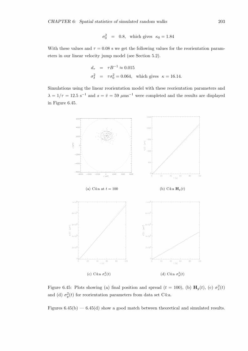
CHAPTER 6: Spatial statistics of simulated random walks 203
σ20 = 0.8, which gives κ0 = 1.84
With these values and τ = 0.08 s we get the following values for the reorientation param-
eters in our linear velocity jump model (see Section 5.2).
dτ = τB−1 ≈ 0.015
σ2δ = τσ2
0 = 0.064, which gives κ = 16.14.
Simulations using the linear reorientation model with these reorientation parameters and
λ = 1/τ = 12.5 s−1 and s = v = 59 µms−1 were completed and the results are displayed
in Figure 6.45.
(a) C4:a at t = 100 (b) C4:a Hy(t)
(c) C4:a σ2
x(t) (d) C4:a σ2
y(t)
Figure 6.45: Plots showing (a) final position and spread (t = 100), (b) Hy(t), (c) σ2x(t)
and (d) σ2y(t) for reorientation parameters from data set C4:a.
Figures 6.45(b) — 6.45(d) show a good match between theoretical and simulated results.

CHAPTER 6: Spatial statistics of simulated random walks 204
6.5.3.2 Data set C4:b
The alternative results obtained from the data after fitting a straight line by linear regres-
sion through the data points for values of τs ≤ 0.4 s only are as follows
B−1 = 0.61,
σ20 = 2.8, which gives κ0 = 0.51.
With these values and τ = 0.08 s we get the following values for the reorientation param-
eters in our linear velocity jump model (see Section 4.2).
dτ = τB−1 ≈ 0.05,
σ2δ = τσ2
0 = 0.224, which gives κ = 5.03.
Simulations using the linear reorientation model with these reorientation parameters and
λ = 1/τ = 12.5 s−1 and s = v = 59 µms−1 were completed and the results are displayed
in Figure 6.46.
Figures 6.46(b) — 6.46(d) show a good match between theoretical and simulated results.
Comparing the results for the two data sets C4:a and C4:b, we see that similarly to data
sets C1 and C3, the spatial statistics are different, with the difference in the spread being
even more significant with this data set. As in the previous cases, the mean position
Hy(t) is similar for both C4:a and C4:b, but the spread is significantly larger for data set
C4:a (which has the larger reorientation parameter κ). This corresponds to the simulated
results observed previously that if dτ is small, the spread will increase as κ increases.
The difference in spread between data sets C4:a and C4:b is more significant than the
differences observed in data sets C1 and C3, because the difference in the values of the
reorientation parameter κ is larger. As with data sets C1 and C3, by looking at both
the spatial and angular statistics of experimental data it should be possible to distinguish
between populations moving with the two different sets of reorientation parameters.
Assuming our velocity jump process model is a reasonable approximation of how a pop-
ulation of the algae C. nivalis moves, then our theory and simulations can give us useful
results to look for in any future experiments. Irrespective of which of the two parameter
estimates used, the algae with gyrotactic motion (sinusoidal model) appear to move less
far than the algae with phototactic motion (linear model), while the phototactic motion
produces the largest displacement with the more intense light (200 klux).
6.6 Conclusions
In this chapter we have presented a computer algorithm to simulate the movement of a
population of random walkers moving with either the linear or sinusoidal velocity jump

CHAPTER 6: Spatial statistics of simulated random walks 205
(a) C4:b at t = 100 (b) C4:b Hy(t)
(c) C4:b σ2
x(t) (d) C4:b σ2
y(t)
Figure 6.46: Plots showing (a) final position and spread (t = 100), (b) Hy(t), (c) σ2x(t)
and (d) σ2y(t) for reorientation parameters from data set C4:b.

CHAPTER 6: Spatial statistics of simulated random walks 206
process models introduced in Chapters 4 and 5. Using these simulations, it is possible to
test the validity of the theoretical equations for the spatial statistics derived in Chapters
4 and 5. In general there is good agreement between simulation and theoretical results,
although as expected the theoretical model does start to break down at extreme values of
the allowed reorientation parameter range for dτ and κ.
In general, the mean position in the preferred direction, Hy(t) always increases as the
reorientation parameters increase up to a maximum limit where the motion is a straight
line in the preferred direction. For the same parameter values, the linear model produces
a greater displacement in the preferred direction than the sinusoidal model.
For a particular value of the parameter κ, the spread about the mean position in either
direction is always larger for the smaller values of dτ (less bias). For a fixed non-zero
value of dτ , the spread increases as κ increases up to a maximum value and then starts to
decrease towards zero, the limiting value that corresponds to motion in a straight line in
the preferred direction. If dτ = 0 then we have an unbiased but correlated random walk
similar to Bovet & Benhamou (1988), and the spread about the mean position is the same
as the spread about the origin and will increase up to a limiting value (given by s2t2) as
κ increases.
A useful application of the simulation model has been to complete simulations with pa-
rameter values from the experiments of Hill & Hader. Although populations of walkers
moving with two different sets of reorientation parameters can have the same long-time
angular distribution and similar values for the mean position Hy(t), the spatial spread
σ2(t) can be significantly different between the two populations if there is a large differ-
ence between the values of the two concentration parameters (κ) that correspond to the
spread in the reorientation distributions. This may prove to be a useful result to use if
analysing experimental data and (as in Hill & Hader’s results) it is hard to distinguish
which set of parameters are appropriate for a particular population of random walkers.
The main results of this chapter are summarised below:
• A computer algorithm has been designed to simulate and analyse the movement of
a population of random walkers all moving with the velocity jump process models
with sinusoidal or linear reorientation as introduced in Chapters 4 and 5.
• In general, there is a good match between the theoretical and simulated results for
all the spatial statistics of interest for most of the parameter values in the range
investigated.
• For more extreme parameter values in the range, the models start to break down
— in particular the asymptotic solution for the sinusoidal model for Hy(t) and
the asymptotic solutions for both reorientation models for the spread in the non-
preferred direction D2y(t), seem to produce unrealistic results for extreme values of
the parameters.

CHAPTER 6: Spatial statistics of simulated random walks 207
• The mean position Hy(t) will increase as the reorientation parameters both increase,
up to a maximum value corresponding to straight line motion (st).
• The average spread about the origin in the non-preferred direction is the same as
the spread about the mean position, D2x(t) = σ2
x(t), since Hx = 0. If dτ = 0 the
spread always increases as κ increases up to a limiting value (s2t2/2). If dτ 6= 0 then
as κ increases, the spread initially increases before reaching a maximum value and
then decreases to zero. For a particular value of κ the spread is greater for smaller
values of dτ .
• The average spread about the origin in the preferred direction D2y(t) increases as
both the reorientation parameters increase, up to a maximum value corresponding
to straight line motion (s2t2).
• The average spread about the mean position in the preferred direction σ2y(t), be-
haves in a similar manner to σ2x(t). If dτ 6= 0 then as κ increases, the spread initially
increases before reaching a maximum value and then decreases to zero. For a partic-
ular value of κ the spread is greater for smaller values of dτ . For the same parameter
values, σ2x(t) > σ2
y(t).
• By analysing the spatial statistics of experimental data it should be possible to
distinguish between random walks with two different sets of reorientation parameters
that produce the same long-time angular statistics as seen in Hill & Hader (1997).

Chapter 7
Angular statistics and the effect of
sampling length
7.1 Introduction
In the previous chapter we used simulations to test the validity of our asymptotic equations
for the spatial statistics of a population of random walkers as well as to investigate the
effect of the reorientation parameters κ and d0 on the spatial statistics. The fact that
we have a good match between theoretical and simulation results, not only means that
we can be confident our asymptotic equations are valid but also that our simulations
work. In this chapter we revisit the results of Hill & Hader (1997) and investigate how
accurate their method is when using simulation data. One of the problems that they found
when analysing experimental data was noise due to heat convection currents and other
environmental factors, and also the fact that for some experiments they only had a small
number of data points. Both these problems can be avoided by running our simulations,
collecting the angular statistics and then completing a similar analysis to Hill & Hader. We
run simulations using known values for the reorientation parameters, compare simulation
results to theory for the expected long-time absolute angular distribution, and see what
effect changing the sampling length has on the turning angle statistics.
7.2 The long-time absolute angular distribution
Section 1.5 gives details of how Hill & Hader (1997) used a simple model of a random walk
on a circle to derive a Fokker–Planck equation (1.93) for the absolute angular distribution
f(θ). Using the assumption that the following results hold as τ → 0,
µδ(θ, τ) = µ0(θ)τ, (7.1)
σ2δ (θ, τ) = σ2
0(θ)τ, (7.2)
208

CHAPTER 7: Angular statistics and the effect of sampling length 209
so that the mean and variance have a linear dependence on τ and both tend to zero as
τ → 0, the following results were obtained.
Sinusoidal reorientation
Assuming that σ20(θ) = σ2
0 is a constant and that
µ0(θ) = −B−1 sin(θ − θ0) (−π ≤ θ, θ0 < π), (7.3)
where θ0 = 0 is the preferred direction and B is the average reorientation time, the long-
time steady state solution to (1.93 ), the Fokker–Planck equation plus boundary conditions,
is given by
f(θ) = M(θ; θ0, 2/Bσ20) =
1
2πI0(2/Bσ20)
exp
(
2
Bσ20
cos(θ − θ0)
)
, (7.4)
where I0(2
Bσ2
0
) is the modified Bessel function of the first kind and zero order.
Linear reorientation
Assuming that σ20(θ) = σ2
0 is a constant and that
µ0(θ) = −B−1θ (−π ≤ θ < π), (7.5)
where θ0 = 0 is the preferred direction and B is the average reorientation time, the long-
time steady state solution to (1.93 ), the Fokker–Planck equation plus boundary conditions,
is given by
f(θ) = B(λ)e−λθ2
, λ = B−1/σ20 , (7.6)
where B(λ) is the normalization function defined by
B(λ) =
(∫ π
−πe−λθ
2
dθ
)
−1
=√λ(√
πerf(π√λ))
−1. (7.7)
See Section 1.5 for further details.
The experimental results of Hill & Hader (1997) were a reasonable fit to the expected
theoretical distributions but they had a lot of noisy data. Using simulations we can verify
that given a population of walkers moving with certain reorientation parameters, the
expected long-time angular distributions in (7.4) and (7.6) are a reasonable fit to data.
When deriving the asymptotic solution equations for the statistics of interest in Chapters
4 and 5 we assumed that we could approximate the higher order angular moments of
our unknown underlying spatial distribution by higher moments of the long-time angular
distributions in (7.4) and (7.6), see Sections 4.6.1 and 5.3.4.1. Using simulations we can
also verify that these higher moments are small in the parameter range that our asymptotic
solution equations are valid, and the approximation using the moments of (7.4) and (7.6)
is reasonable.

CHAPTER 7: Angular statistics and the effect of sampling length 210
7.2.1 Validating the approximation for M0(t)
When closing the systems of differential equations for the linear reorientation model in
Chapter 5, we approximated the higher order moments F3(t), K3(t), M3(t) and also the
moment M0(t) as time-independent constants using the steady state solution (7.6). Using
simulations we can demonstrate that the approximation for M0(t) as a time-independent
constant is reasonable. Figure 7.1 compares values of M0(t) for simulated data and ap-
proximations using the steady state solution (7.6). Note that assuming there is a uniform
spread of initial directions, M0(0) = π2/3 ≈ 3.29. The simulations have been completed
with three values of κ and all have dτ = 0.2 and λ = 1. It is clear from Figure 7.1 that
Figure 7.1: Plots of M0(t) against t. Legend: (- -) simulation κ = 1, (· · ·) simulation
κ = 2, (− · −) simulation κ = 4, (+) approximation κ = 1, (*) approximation κ = 2, (♦)
approximation κ = 4.
the simulated values reach a steady state very quickly. Thus, although the approxima-
tions using Hill & Hader’s steady state solution, (7.6), seem to slightly underestimate the
simulated values, it seems reasonable to approximate M0(t) as a time-independent con-
stant as we have done in Chapter 5. The reason for this slight underestimation of the
simulation results is discussed later in this chapter and seems likely to be because Hill &
Hader’s steady state approximation, (7.6), is valid for continuous random walks. If we
use a smaller time step between turns (larger value of λ) then the approximations become
closer to the simulated results, although the simulations now take longer to reach the
steady state solutions.
7.2.2 Comparing theoretical distributions to simulation results
For the following results we have run simulations of 2000 walkers moving for 500 time
steps, where each time step τ = 0.1 s, and the reorientation parameters are taken from

CHAPTER 7: Angular statistics and the effect of sampling length 211
Hill & Hader’s experimental results so that we can make direct comparisons with their
data.
7.2.2.1 Sinusoidal reorientation
Plots of the long-time angular distribution using parameters from Hill & Hader’s experi-
mental results with data set C1 are shown in Figure 7.2. Data set C1 is the set of data
collected on algae moving with sinusoidal reorientation due to gyrotaxis, set C1:a being
the reorientation parameter values estimated using all sampling time steps, and set C1:b
being the reorientation parameter values estimated using only sampling time steps for
τs ≤ 0.4 s (see Section 1.5.3).
Simulation p.d.f.Theoretical p.d.f.
Legend
0
0.05
0.1
0.15
0.2
0.25
0.3
–3 –2 –1 1 2 3θ
(a) C1:a : κ0 = 0.95, B−1 = 0.37.
Simulation p.d.f.Theoretical p.d.f.
Legend
0
0.05
0.1
0.15
0.2
0.25
0.3
–3 –2 –1 1 2 3θ
(b) C1:b : κ0 = 0.27, B−1 = 0.8.
Figure 7.2: Plots showing theoretical and simulated long-time p.d.f., f(θ), with parameter
values taken from Hill and Hader’s experiments with data set C1.
Both sets of parameter values produce the same long-time theoretical probability distri-
bution for f(θ). This is expected since Hill & Hader used the observed long-time angular
distribution from experiments to estimate σ20 given two different estimates of B−1 (Section
1.5.3). Even with 2000 data points our simulation data is fairly noisy, but the simulated
results seem a reasonable fit to the theoretical distribution. It would be possible to do
various tests to see how good the fit between theory and simulation is (see for example,
Fisher (1993), or Mardia & Jupp (1999)), but for our purposes, it is easier to compare by
looking at the moments of the distributions as we do in the next section.

CHAPTER 7: Angular statistics and the effect of sampling length 212
7.2.2.2 Linear reorientation
Plots of the long-time angular distribution using parameters from Hill & Hader’s exper-
imental results with data set C3 and C4 are shown in Figures 7.3 and 7.4 respectively.
Data set C3 is the set of data collected on algae moving with linear reorientation due to
phototaxis with an 80 klux light source, while C4 is the set of data collected on algae
moving with linear reorientation due to phototaxis with a 200 klux light source. Sets
C3:a and C4:a are the reorientation parameter values estimated using all sampling time
steps, and set C3:b and C4:b are the reorientation parameter values estimated using only
sampling time steps for τs ≤ 0.4 s (see Section 1.5.3).
Simulation p.d.f.Theoretical p.d.f.
Legend
0
0.05
0.1
0.15
0.2
0.25
0.3
–3 –2 –1 1 2 3θ
(a) C3:a : κ0 = 0.41, B−1 = 0.44.
Simulation p.d.f.Theoretical p.d.f.
Legend
0
0.05
0.1
0.15
0.2
0.25
0.3
–3 –2 –1 1 2 3θ
(b) C3:b : κ0 = 0.22, B−1 = 0.62.
Figure 7.3: Plots showing theoretical and simulated long-time p.d.f., f(θ), with parameter
values taken from Hill and Hader’s experiments with data set C3.
As with the sinusoidal model, sets C3:a and C3:b, and C4:a and C4:b produce the same
long-time theoretical probability distribution for f(θ) respectively.
As with the sinusoidal model, there is a reasonable fit between simulation and theoretical
results. We will comment more on the fit by looking at the moments of the distributions
in the next section.
7.2.2.3 Limitations of the theoretical model
The previous simulations were completed with a time step of τ = 0.1 s and produced a
reasonable fit between theoretical and simulation results. Since τ = 0.1 s, the variance
of the turning angle was small, σ2δ = 0.1σ2
0 . The solutions for the long-time angular
distributions in (7.4) and (7.6) are independent of τ since dτ/σ2δ = B−1/σ2
0 , and predict

CHAPTER 7: Angular statistics and the effect of sampling length 213
Simulation p.d.f.Theoretical p.d.f.
Legend
0
0.05
0.1
0.15
0.2
0.25
0.3
–3 –2 –1 1 2 3θ
(a) C4:a : κ0 = 1.84, B−1 = 0.19.
Simulation p.d.f.Theoretical p.d.f.
Legend
0
0.05
0.1
0.15
0.2
0.25
0.3
–3 –2 –1 1 2 3θ
(b) C4:b : κ0 = 0.51, B−1 = 0.61.
Figure 7.4: Plots showing theoretical and simulated long-time p.d.f., f(θ), with parameter
values taken from Hill and Hader’s experiments with data set C4.
the same theoretical distribution for all values of τ . However when deriving the Fokker–
Planck equation, Hill & Hader made the assumption that (7.3) and (7.5) hold only as
τ → 0.
The following simulations have been run with the same values for σ20 and B−1 but with
τ = 1 s. Thus, there is now a large variance in the turning angle σ2δ when compared to
the previous section.
Figure 7.5 show plots of the long-time angular distribution for data set C1, while Figure
7.6 show the distribution for data set C4, both completed with simulations with τ = 1 s.
From Figures 7.5 and 7.6, it is clear that the simulated data is now not a good fit to
the theoretical expected long-time angular distribution. The fit seems to be worse for
the smaller κ values corresponding to a large value of σ2δ . This makes sense — if one
increased the time step used by each walker so that σ2δ became very large, then at some
point the variance of the turning angle at each step would be greater than the variance of
the expected long-time angular distribution.
This is obviously nonsensical — consider the unlikely situation of a population all facing
the preferred direction after a long-time period. After one further time step all walkers will
now be distributed according to the turning angle distribution and have a larger variance
than the expected theoretical absolute angle distribution. If the walkers start with a
distribution that is not all facing the preferred direction then the subsequent variance
after one step will be even greater. This result is confirmed when looking at the moments
of the long-time angular distribution in the next section.

CHAPTER 7: Angular statistics and the effect of sampling length 214
Simulation p.d.f.Theoretical p.d.f.
Legend
0
0.05
0.1
0.15
0.2
0.25
0.3
–3 –2 –1 1 2 3θ
(a) C1:a : κ0 = 0.95, B−1 = 0.37.
Simulation p.d.f.Theoretical p.d.f.
Legend
0
0.05
0.1
0.15
0.2
0.25
0.3
–3 –2 –1 1 2 3θ
(b) C1:b : κ0 = 0.27, B−1 = 0.8.
Figure 7.5: Plots showing theoretical and simulated long-time p.d.f., f(θ), for data set C1
with τ = 1.
Simulation p.d.f.Theoretical p.d.f.
Legend
0
0.05
0.1
0.15
0.2
0.25
0.3
–3 –2 –1 1 2 3θ
(a) C4:a : κ0 = 1.84, B−1 = 0.19.
Simulation p.d.f.Theoretical p.d.f.
Legend
0
0.05
0.1
0.15
0.2
0.25
0.3
–3 –2 –1 1 2 3θ
(b) C4:b : κ0 = 0.51, B−1 = 0.61.
Figure 7.6: Plots showing theoretical and simulated long-time p.d.f., f(θ), for data set C4
with τ = 1.

CHAPTER 7: Angular statistics and the effect of sampling length 215
7.2.3 Moments of the long-time absolute angular distribution
From Section 1.2 the angular moments of a circular distribution f(θ) are given by
an =
∫ π
−πcos(nθ)f(θ) dθ, bn =
∫ π
−πsin(nθ)f(θ) dθ, (7.8)
where bn = 0 ∀n if the distribution is symmetric about θ = 0. We are interested in the
moments for n ≤ 4, corresponding to the moments we defined for our unknown underlying
spatial distribution Fn(t) in (4.15). The moments F3 and F4 were assumed to be time
independent and approximated by a3 and a4, the moments of the expected long-time
angular distribution f(θ) from (7.4) and (7.6) in order to close our system of differential
equations, see Section 4.6.1.
From Section 4.6.1, the angular moments for the expected long-time angular distribution
with sinusoidal reorientation are simply
an =In(z)
I0(z), (7.9)
where z = 2/Bσ20 . The angular moments for the expected long-time angular distribution
with linear reorientation are not as simple and are given in Section 5.3.4.1.
In the following simulations we have calculated the simulated angular moments using
an =1
N
N∑
i=1
cosnθF,i, (7.10)
where each simulation is run with N = 2000 walkers, and θF,i is the final angle of facing
of the i-th walker.
7.2.3.1 First angular moment, n = 1
The plots in Figures 7.7 and 7.8, show how the first angular moment a1 changes as the
concentration parameter for unit time κ0 increases, for sinusoidal and linear reorientation
respectively. Two different plots show results for B−1 = 0.1 and B−1 = 0.5, while each
plot shows the theoretical result, the simulated result using a time step of τ = 0.1 s, and
the simulated result using a time step of τ = 1 s. The latter will thus have a much larger
variance in the turning angle σ2δ (and a larger value of B−1).
Figures 7.7 and 7.8 confirm the main result observed in the previous section — the simu-
lated results for τ = 0.1 s are a reasonable fit to the theoretical expected angular moments,
but the simulated results for τ = 1 s are consistently smaller than the theoretical expected
moments, with the greatest difference being when κ0 is small corresponding to a large
variance in the turning angle distribution. In general, a1 is larger for the linear model
for the same reorientation parameters — this corresponds to the linear model giving a
larger absolute displacement as observed in previous chapters (the moment a1 is the same
moment that results in the equation for the absolute velocity Vy(t) in previous chapters).

CHAPTER 7: Angular statistics and the effect of sampling length 216
(a) a1 , B−1 = 0.1 (b) a1, B−1 = 0.5
Figure 7.7: Plots showing the first angular moment a1 against k0 for the sinusoidal re-
orientation model, with (a) B−1 = 0.1, (b) B−1 = 0.5. Legend: theoretical results (—),
simulation results with τ = 0.1 s (- -), simulation results with τ = 1 s (· · ·).
(a) a1 , B−1 = 0.1 (b) a1, B−1 = 0.5
Figure 7.8: Plots showing the first angular moment a1 against k0 for the linear reorientation
model, with (a) B−1 = 0.1, (b) B−1 = 0.5. Legend: theoretical results (—), simulation
results with τ = 0.1 s (- -), simulation results with τ = 1 s (· · ·).

CHAPTER 7: Angular statistics and the effect of sampling length 217
Similar results are obtained for the angular moment a2; the results are not presented as
we have made no previous assumptions about this moment in our analysis in Chapters 4
and 5.
7.2.3.2 Third angular moment, n = 3
The plots in Figure 7.9 show how the third angular moment a3 changes as the concentration
parameter for unit time κ0 increases and B−1 = 0.5, for sinusoidal and linear reorientation
respectively. Each plot shows the theoretical result, the simulated result using a time step
of τ = 0.1 s, and the simulated result using a time step of τ = 1 s.
(a) Sinusoidal a3 , B−1 = 0.5 (b) Linear a3, B−1 = 0.5
Figure 7.9: Plots showing the third angular moment a3 against k0 with B−1 = 0.5, for (a)
sinusoidal reorientation model (b) linear reorientation model. Legend: theoretical results
(—), simulation results with τ = 0.1 s (- -), simulation results with τ = 1 s (· · ·).
When B−1 = 0.1 the simulated and theoretical values of a3 ≈ 0, and there is a large
amount of relative noise in the simulation data. For this reason results are not shown.
The plots shown in Figure 7.9 show similar results to that seen with the moment a1 —
there is a reasonable fit between the theoretical results and simulations with τ = 0.1
s, but the theoretical solutions overestimate the simulation results when τ = 1 s. In
general, the higher moment a3 is relatively small even with large values of the reorientation
parameters — it seems that our approximation using Hill & Hader’s long-time expected
angular distribution for the higher moments in our system derived in the previous chapters
is reasonable. For the same reorientation parameter values, the linear model has a higher
value of a3.

CHAPTER 7: Angular statistics and the effect of sampling length 218
7.2.3.3 Fourth angular moment, n = 4
The plots in Figure 7.10 show how the fourth angular moment a4 changes as the con-
centration parameter for unit time κ0 increases and B−1 = 0.5, for sinusoidal and linear
reorientation respectively. Each plot shows the theoretical result, the simulated result
using a time step of τ = 0.1 s, and the simulated result using a time step of τ = 1 s.
(a) Sinusoidal a4 , B−1 = 0.5 (b) Linear a4, B−1 = 0.5
Figure 7.10: Plots showing the fourth angular moment a4 against k0 with B−1 = 0.5,
for (a) sinusoidal reorientation model (b) linear reorientation model. Legend: theoretical
results (—), simulation results with τ = 0.1 s (- -), simulation results with τ = 1 s (· · ·).
The plots in Figure 7.10 show similar results to those in Figure 7.9 and the same comments
apply. For the same reorientation parameter values and allowing for simulation noise,
a3 > a4 for both reorientation models.
The long-time expected angular distributions of Hill & Hader, (7.4) and (7.6), are only
likely to be a reasonable fit to experimental or simulation data if the time step used by
the walkers τ is small and the subsequent variance of the turning angle distribution is
also small. If we have a large value for dτ and σ2δ then the moments of the theoretical
distribution will overestimate the true angular moments.
There is a reasonable fit between simulation and theory for the higher order moments that
we approximated in Section 4.6.1. However, in Section 4.6.1 we also made the assumption
that the approximations were time independent and so for small time they may not be as
valid. In general these higher moments are approximately zero except for large values of the
reorientation parameters and this is unlikely to affect our asymptotic solution equations
(as the results in Chapter 6 suggest).

CHAPTER 7: Angular statistics and the effect of sampling length 219
7.3 The effect of sampling length on the angular statistics
of a velocity jump process
In the following analysis of the angular statistics of random walks we refer to the sampling
length, τs, as the fixed time between observations of the spatial position of each trajectory.
By changing the sampling length we change the time between observations — this results
in a linear interpolation of the original trajectory data for each sampling length.
Recall the assumption made by Hill & Hader that, as τ → 0,
µδ(θ, τ) = µ0(θ)τ,
σ2δ (θ, τ) = σ2
0(θ)τ.
Using this assumption Hill & Hader applied different sampling lengths, τs, to their data
and calculated the parameter µ0 for each value of τs. Assuming the linear dependence
on τs they were able to extrapolate back and estimate the value of B−1. This resulted in
two different estimates for B−1, depending on whether they used all values of τs or just
those values such that τs ≤ 5τ (where τ is the average of the observed time step between
turns subject to the limitations of the experimental set-up), see Section 1.5. They knew
that the assumption that the observed value of µδ(θ, τ) = µ0(θ)τs was only valid for small
τs, but their data was quite noisy hence the two possible estimates for B−1. Using these
estimates and the observed long-time angular distribution, they were able to use (7.4) and
(7.6) to estimate the parameter σ20 .
It is possible to repeat the method of Hill & Hader using simulations with a lot more data
and with reorientation parameters that we fix for the whole population of walkers. Thus,
we can compare the known reorientation parameters that were used in the simulations to
the reorientation parameters that are calculated using Hill & Hader’s method.
It should be made clear that from now on when we refer to τ we mean the time step
between turns used by the population of walkers in the original random walk. When we
refer to τs we mean the new time step between points on the trajectories imposed by
changing the sampling length.
When changing the sampling length we use a linear interpolation of the spatial position
at each time step. The algorithm is given in Section 7 of Hill & Hader (1997). Using
this simple linear interpolation the observed spatial statistics will be unchanged, but the
angular statistics will be different. In a biased random walk, Hill & Hader predicted that
as τs → ∞, the p.d.f. of the direction of movement, θ, will become more peaked about
the preferred direction, with a consequent reduction in the mean turning angle µδ(τs)
(averaged over all swimming directions) and thus in σ2δ (τs). This is clearer when looking
at the example plots in the next section.

CHAPTER 7: Angular statistics and the effect of sampling length 220
7.3.1 Examples of changing the sampling length
Figure 7.11(a) shows an individual random walk using the sinusoidal simulation model
(where the turning rate is given by a Poisson process with parameter λ) for 500 time
steps, with s = λ = 1 and reorientation parameters κ = 1 and dτ = 0.3. Figures 7.11(b)—
(f), show the same random walk rediscretized with different fixed sampling lengths.
It is clear from Figure 7.11 that as τs increases the observed speed decreases and the total
distance travelled appears less, although the overall absolute displacement is the same.
Increasing the sampling length, τs, has the effect of smoothing out the trajectory and a
lot of information about the original random walk is lost.
7.3.2 Angular statistics of a velocity jump process with sinusoidal re-
orientation
For the following study we ran the velocity jump process simulation with sinusoidal reori-
entation for 200 time steps with a population of 2500 walkers. Thus, for a unit sampling
length we would expect approximately 500,000 turning angles to collect statistics from
(Hill & Hader had only approximately 5000 turning angles to work with and encountered
problems with small numbers of data points with large sampling lengths). The simulation
has been run with ‘typical’ parameters from Hill & Hader’s experimental results. We as-
sume that τ = 0.08 s, B−1 = 0.6, and σ20 = 2, so that in the simulations we use dτ = 0.05,
σ2δ ≈ 0.2 and correspondingly κ = 6. These parameter values are comparable to the values
in data sets C1 — C4 from Hill & Hader, see Section 1.5.3. As we are only interested in the
angular statistics, we assume that we can rescale with respect to time so that s = λ = 1
for convenience (Section 4.9.2).
Using the data from this simulation run we then apply different sampling lengths τs and
calculate a new set of absolute angles (θ) and corresponding turning angles (δ) for each
sampling length. Each new set of absolute angles is split into 18 bins of size π9 rads, and for
each bin we calculate the mean turning angle µδ(θ) and angular variance σ2δ (θ). Sampling
lengths of less than τ/2 are not used to avoid spurious correlations.
Recall from (7.3), that we expect µδ(θ) = −dτs sin θ and σ2δ (θ) = σ2
δ = constant. Using
the assumption that µδ(θ, τ) decreases linearly as τ decreases we can then calculate an
estimate for B−1, which should be the gradient of the graph of dτs plotted against τs (and
we might expect to find B−1 = 0.05). This is exactly the method used by Hill & Hader
so we are able to compare results.
7.3.2.1 Mean turning angle, µδ(θ)
Plots showing µδ(θ) against θ for various sampling lengths τs are shown in Figure 7.12.
Other sampling lengths were also used but plots are omitted — see Table 7.1.
Hill & Hader encountered a lot of noise in their experimental results and also had only

CHAPTER 7: Angular statistics and the effect of sampling length 221
(a) Poisson time step (λ = 1). (b) τs = 1.
(c) τs = 2. (d) τs= 5.
(e) τs = 10. (f) τs = 50.
Figure 7.11: Plots showing the effect of changing the sampling length τs of an individual
random walk.

CHAPTER 7: Angular statistics and the effect of sampling length 222
(a) τs = 0.6τ (b) τs = τ (c) τs = 2τ
(d) τs = 5τ (e) τs = 10τ (f) τs = 20τ
Figure 7.12: Plots showing how µδ(θ) changes with θ for the sinusoidal model with various
sampling lengths τs. Simulation results for angular bins of π9 rads (—), and functions fitted
by inspection to the data (- -).

CHAPTER 7: Angular statistics and the effect of sampling length 223
a small number of data points for larger sampling lengths. Consequently, they used a
method of least squares to fit a sinusoidal function to their data. In the plots displayed in
Figure 7.12, we have simply fitted a sinusoidal function by inspection — this is reasonable
as there seems to be little noise in the data (except for τs = 20).
7.3.2.2 Variance of the turning angle, σ2δ (θ)
Plots showing σ2δ (θ) against θ for various sampling lengths τs are shown in Figure 7.13.
Other sampling lengths were also used but plots are omitted — see Table 7.1.
(a) τs = 0.6τ (b) τs = τ (c) τs = 2τ
(d) τs = 5τ (e) τs = 10τ (f) τs = 20τ
Figure 7.13: Plots showing how σ2δ (θ) changes with θ for the sinusoidal model with various
sampling lengths τs. Simulation results for angular bins of π9 rads (—), and the mean from
the data averaging over all θ (- -).
In the above plots the straight line plotted is the mean of the variance, σ2δ (θ), averaged
over all angles, which Hill & Hader assumed to be a constant. It is clear however, that
for larger sampling lengths the variance is not constant over θ, but small for θ ≈ 0
and significantly larger for θ ≈ ±π. Hill & Hader also encountered this effect in their
experimental results and suggested that there was possibly a weak sinusoidal dependence
of the form σδ(θ) = a− b sin θ. However, from the above (and subsequent) results, if σ2δ (θ)

CHAPTER 7: Angular statistics and the effect of sampling length 224
is a constant for the original random walk but the sampling length is such that τs ≫ τ
then the variance of the turning angle will become small close to θ = 0 and large close to
θ = ±π. It seems likely that this is the effect observed by Hill & Hader and this suggests
that their sampling length was too large (although it was not possible for them to sample
at shorter time scales due to experimental constraints).
A possible explanation for this effect is as follows: walkers that are moving close to the
preferred direction (θ ≈ 0) will become increasingly likely to still be orientated towards
the preferred direction as the sampling length increases, and thus there will be a small
relative variance in σ2δ (θ) for θ ≈ 0. However, a walker moving opposite to the preferred
direction (θ ≈ ±π) will become increasingly likely to turn towards the preferred direction
as the sampling length increases, and this seems to introduce a large relative variance in
σ2δ (θ) for θ ≈ ±π. As suggested by Hill & Hader, if the sampling length of a correlated
and biased random walk keeps on increasing then eventually we would expect to observe a
decrease in the variance of the turning angle as almost every turn will be back towards the
preferred direction — this is observed in later results. Bovet & Benhamou (1988) showed
that if the sampling length of a correlated but unbiased random walk keeps on increasing
then the variance of the turning angle tends to infinity and the walk appears completely
random (Brownian) and all correlation effects are lost.
7.3.2.3 Estimating the reorientation parameters
Table 7.1 shows the amplitude of the functions fitted by inspection for the plots of µδ(θ)
v θ, and the values of the mean calculated over all θ for σ2δ for the sinusoidal model.
τs/τ 0.6 1 2 3 4 5 6
dτs 0.02 0.03 0.06 0.09 0.12 0.15 0.18
σ2δ 0.09 0.15 0.29 0.49 0.59 0.72 0.89
τs/τ 8 10 12 14 16 18 20
dτs 0.24 0.28 0.37 0.42 0.49 0.55 0.60
σ2δ 1.17 1.41 1.73 1.98 2.21 2.41 2.51
Table 7.1: Estimated value for the amplitude of the mean turning angle µδ(θ), and calcu-
lated mean value of σ2δ , for the sinusoidal model with rescaled sampling length τs/τ .
The data from Table 7.1 is plotted in Figure 7.14. In each plot the observed values
from Table 7.1 are represented by a dashed line (- -), and the expected value by a solid
line (—). The expected value is simply calculated from the reorientation parameters
used in the original simulation (including τ = 0.1) so that E(dτs) = B−1τs = 0.5τs and
E(σ2δ (τs)) = σ2
0τs = 2τs.
From Figure 7.14(a) it appears that for the sampling lengths we have used the observed

CHAPTER 7: Angular statistics and the effect of sampling length 225
(a) dτsv τs/τ (b) σ2
δ v τs/τ
Figure 7.14: Plots showing (a) the amplitude of the mean turning angle dτs , (b) variance
of the turning angle σ2δ , against rescaled sampling length τs/τ for the sinusoidal model.
reorientation parameter dτs does increase linearly as the sampling length increases. The
gradient of the plot appears linear for all values of τs unlike the results of Hill & Hader
that appeared to level off if the sampling length was too large. The value of B−1 estimated
from the gradient of the observed values (and recalling that τ = 0.1) is given by
B−1 = dτs/τs = 0.3. (7.11)
So the assumption made by Hill & Hader that the observed reorientation parameter dτs
increases linearly with τs appears to hold for these sampling lengths but the gradient
calculated from these observed values, B−1 = 0.3, underestimates the expected value,
B−1 = 0.5.
From Figure 7.14(b) it can be seen that the mean variance in the turning angle σ2δ increases
linearly with τs only for small values of τs, and for larger values the increase is non-linear
and appears to level off. This fits with the previous argument and Hill & Hader’s comment
that the variance in the turning angle will start to decrease if the sampling length is large
enough. As with the estimate of dτs , the value of σ20 estimated from the gradient of the
plot for small τs, given by
σ20 = σ2
δ/τs ≈ 1.5, (7.12)
is also an underestimate of the known variance used in the original simulation, σ20 = 2.
Even if we use a sampling length of τs = τ so that we are sampling with the same average
time between turns as the original trajectory, we still underestimate the known value of dτ
and σ2δ that we know the walkers are using. Recall that our velocity jump process model
uses a Poisson process to model the time between turns, where τ is only the average time
between turns. It seems likely that by applying a fixed sampling length to the Poisson time

CHAPTER 7: Angular statistics and the effect of sampling length 226
steps in the original random walk some smoothing of the trajectory will have taken place
and/or some ‘turns’ will be wrongly recorded as δ = 0 if a particular part of a trajectory
is in the same direction for a larger time than the sampling length. This could explain
why using a unit sampling length (τs = τ) underestimates the reorientation parameters.
However, as we shall see later in Section 7.4.1, this does not completely explain why at
larger sampling lengths the reorientation parameters are underestimated.
7.3.3 Angular statistics of a velocity jump process with linear reorien-
tation
We use the same simulation parameters and method as described in Section 7.3.2 to look
at the effect of the sampling length on the angular statistics of a velocity jump process with
linear reorientation. Recall from (7.3), that we expect µδ(θ) = −dτsθ and σ2δ (θ) = σ2
δ =
constant. Using the assumption that dτs and σ2δ decrease linearly with τs we can estimate
the reorientation parameters from the observed data exactly as Hill & Hader did.
7.3.3.1 Mean turning angle, µδ(θ)
Plots showing µδ(θ) against θ for various sampling lengths τs are shown in Figure 7.15.
Other sampling lengths were also used but plots are omitted — see Table 7.2.
As for the sinusoidal model, in the plots displayed in Figure 7.12 we have simply fitted a
linear function by inspection — this is reasonable as there seems to be little noise in the
data (except for θ ≈ ±π). It would be possible to use a method of least squares as Hill &
Hader did with their data but this seems unnecessary for the level of accuracy we require.
7.3.3.2 Variance of the turning angle, σ2δ (θ)
Plots showing σ2δ (θ) against θ for various sampling lengths τs are shown in Figure 7.16.
Other sampling lengths were also used but plots are omitted — see Table 7.2.
The plots in Figure 7.16 show similar behaviour to the sinusoidal model — the variance
in the turning angle is independent of θ for small sampling lengths, but at large sampling
lengths the variance is much greater when θ ≈ ±π compared to the variance when θ ≈ 0.
Possible reasons for this have been discussed previously.
7.3.3.3 Estimating the reorientation parameters
Table 7.2 shows the amplitude of the functions fitted by inspection for the plots of µδ(θ)
v θ, and the values of the mean calculated over all θ for σ2δ for the linear reorientation
model.
The data from Table 7.2 is plotted in Figure 7.17. In each plot the observed values
from Table 7.2 are represented by a dashed line (- -), and the expected value by a solid
line (—). The expected value is simply calculated from the reorientation parameters
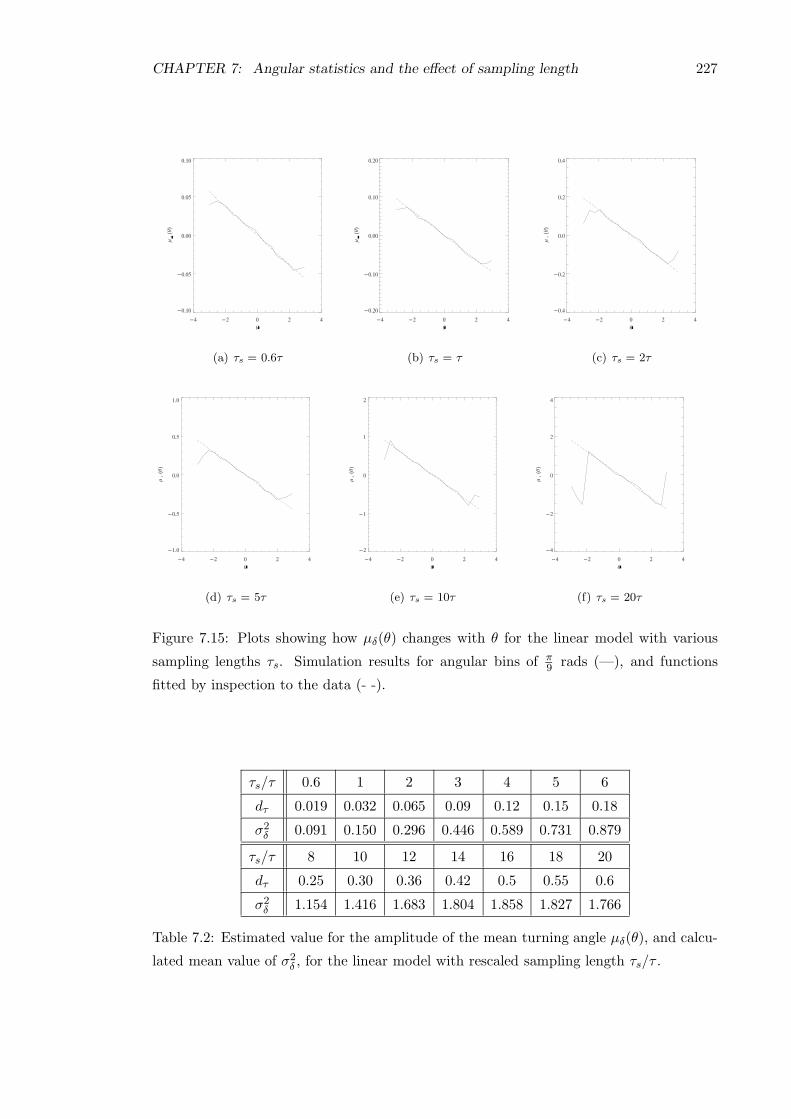
CHAPTER 7: Angular statistics and the effect of sampling length 227
(a) τs = 0.6τ (b) τs = τ (c) τs = 2τ
(d) τs = 5τ (e) τs = 10τ (f) τs = 20τ
Figure 7.15: Plots showing how µδ(θ) changes with θ for the linear model with various
sampling lengths τs. Simulation results for angular bins of π9 rads (—), and functions
fitted by inspection to the data (- -).
τs/τ 0.6 1 2 3 4 5 6
dτ 0.019 0.032 0.065 0.09 0.12 0.15 0.18
σ2δ 0.091 0.150 0.296 0.446 0.589 0.731 0.879
τs/τ 8 10 12 14 16 18 20
dτ 0.25 0.30 0.36 0.42 0.5 0.55 0.6
σ2δ 1.154 1.416 1.683 1.804 1.858 1.827 1.766
Table 7.2: Estimated value for the amplitude of the mean turning angle µδ(θ), and calcu-
lated mean value of σ2δ , for the linear model with rescaled sampling length τs/τ .

CHAPTER 7: Angular statistics and the effect of sampling length 228
(a) τs = 0.6τ (b) τs = τ (c) τs = 2τ
(d) τs = 5τ (e) τs = 10τ (f) τs = 20τ
Figure 7.16: Plots showing how σ2δ (θ) changes with θ for the linear model with various
sampling lengths τs. Simulation results for angular bins of π9 rads (—), and the mean from
the data averaging over all θ (- -).

CHAPTER 7: Angular statistics and the effect of sampling length 229
used in the original simulation (including τ = 0.1) so that E(dτs) = B−1τs = 0.5τs and
E(σ2δ (τs)) = σ2
0τs = 2τs.
(a) dτsv τs/τ (b) σ2
δ v τs/τ
Figure 7.17: Plots showing (a) the amplitude of the mean turning angle dτs , (b) variance
of the turning angle σ2δ , against rescaled sampling length τs/τ for the linear model.
From Figure 7.17 we have very similar behaviour to the results observed from the sinusoidal
model. From Figure 7.17(a), the estimated value of the reorientation parameter is B−1 =
0.3 which underestimates the known value of B−1 = 0.5, and is the same value as observed
in the sinusoidal model.
From Figure 7.17(b), the estimated value of the mean variance of the turning angle for
small sampling lengths, τs < 10τ , is σ20 = 1.5 which underestimates the known value of
σ20 = 2, and is the same value as observed in the sinusoidal model. For large sampling
lengths the mean variance in the turning angle starts to decrease as observed and discussed
previously.
As with the sinusoidal model, the observed values of the reorientation parameters always
underestimate the known reorientation parameters even with a unit sampling length, τs =
τ .
7.4 Limitations of using the angular statistics to estimate
the reorientation parameters of a velocity jump process
In the previous section we have used the method of Hill & Hader to calculate the reori-
entation parameters of a velocity jump process from the observed data from simulations
using different sampling lengths. For small sampling lengths, the assumption made by
Hill & Hader that the amplitude of the mean turning angle, dτs , and the mean variance
of the turning angle, σ2δ , decrease linearly as τs decreases holds. However, even using a

CHAPTER 7: Angular statistics and the effect of sampling length 230
unit sampling length, τs = τ , the observed values of the reorientation parameters seem to
underestimate the known values used in the simulations.
One possible reason for this is that by applying a unit sampling length, τs = τ , to the
trajectory of a random walk where the time between turns is given by a Poisson process
with average τ , we smooth out the data and some information about the random walk is
lost. Another possible reason is that the method of Hill & Hader is only valid when the
original random walk is continuous and by using a velocity jump process as an approxima-
tion in the simulations we cannot accurately estimate the reorientation parameters from
observed data with different sampling lengths.
7.4.1 The effect of sampling length on the angular statistics of a velocity
jump process with a fixed time between turns
To test if the variable Poisson step length in the original random walk causes the under-
estimation of the reorientation parameters, we carry out simulations in exactly the same
manner and using the same parameters as in Section 7.3.2, except we now use a fixed time
step between turns, τ = 0.1.
7.4.1.1 The mean and variance of the turning angle
Example plots showing µδ(θ) and σ2δ (θ) against θ for fixed τ and τs = τ and τs = 10τ , are
shown in Figures 7.18 and 7.19, for the sinusoidal and linear models respectively. Other
sampling lengths were also used but plots are omitted — see Tables 7.3 and 7.4 and Figures
7.20 and 7.21.
From Figures 7.18 and 7.19, it is clear that when we have unit sampling length τs = τ ,
then dτ = 0.05 and σ2δ ≈ 0.2 as we expect. However, for τs = 10τ it appears that the
observed parameter values underestimate the known values used in the simulations, and
the plots are very similar to those observed in the previous section for the same sampling
length.
7.4.1.2 Estimating the reorientation parameters
Tables 7.3 and 7.4 show the amplitude of the functions fitted by inspection for the plots
of µδ(θ) v θ, and the values of the mean calculated over all θ for σ2δ , for the sinusoidal and
linear reorientation models with fixed time between turns respectively.
The data from Tables 7.3 and 7.4 is plotted in Figures 7.20 and 7.21. In each plot the
observed values from Tables 7.3 and 7.4 are represented by a dashed line (- -), and the
expected values by a solid line (—). The expected values are simply calculated from
the reorientation parameters used in the original simulation (where τ = 0.1) so that
E(dτs) = B−1τs = 0.5τs and E(σ2δ (τs)) = σ2
0τs = 2τs.

CHAPTER 7: Angular statistics and the effect of sampling length 231
(a) τs = τ (b) τs = 10τ
(c) τs = τ (d) τs = 10τ
Figure 7.18: Plots showing how µδ(θ) and σ2δ change with θ for the sinusoidal model with
fixed time between turns.
τs/τ 0.6 1 2 5 10 20
dτ 0.024 0.05 0.08 0.16 0.3 0.65
σ2δ 0.095 0.226 0.339 0.773 1.506 2.755
Table 7.3: Estimated value for the amplitude of the mean turning angle µδ(θ), and calcu-
lated mean value of σ2δ , for the sinusoidal model with fixed time between turns and with
rescaled sampling length τs/τ .

CHAPTER 7: Angular statistics and the effect of sampling length 232
(a) τs = τ (b) τs = 10τ
(c) τs = τ (d) τs = 10τ
Figure 7.19: Plots showing how µδ(θ) and σ2δ change with θ for the linear model with fixed
time between turns.
τs/τ 0.6 1 2 5 10 20
dτ 0.02 0.05 0.08 0.17 0.35 0.66
σ2δ 0.010 0.226 0.340 0.773 1.493 1.653
Table 7.4: Estimated value for the amplitude of the mean turning angle µδ(θ), and cal-
culated mean value of σ2δ , for the linear model with fixed time between turns and with
rescaled sampling length τs/τ .

CHAPTER 7: Angular statistics and the effect of sampling length 233
(a) dτsv τs/τ (b) σ2
δ v τs/τ
Figure 7.20: Plots showing (a) the amplitude of the mean turning angle dτs , (b) variance
of the turning angle σ2δ , against rescaled sampling length τs/τ for the sinusoidal model
with fixed time between turns.
(a) dτsv τs/τ (b) σ2
δ v τs/τ
Figure 7.21: Plots showing (a) the amplitude of the mean turning angle dτs , (b) variance
of the turning angle σ2δ , against rescaled sampling length τs/τ for the linear model with
fixed time between turns.

CHAPTER 7: Angular statistics and the effect of sampling length 234
Although estimates of the reorientation parameters from the observed data for a velocity
jump process with fixed τ match the known values of the parameters for a unit sampling
length τs = τ , the subsequent behaviour as the sampling length increases is very similar
to that observed in a velocity jump process with variable τ , see Figures 7.14 and 7.17.
From the observed data, the estimates of the reorientation parameters using sampling
lengths larger than the unit length, τs > τ , always underestimate the known values used
in the simulations. It appears that if observing experimental/simulation data from a
velocity jump process with a fixed time between turns, the estimates for the values of the
reorientation parameters underestimate the true values, unless the sampling length used
is the same as the time between turns of the original random walk.
7.4.2 Estimating the reorientation parameters for large and small values
of τ and τs
A possible explanation for the fact that our estimates of the reorientation parameters
using observed data from simulated velocity jump processes, is that the method of Hill &
Hader only holds for a continuous random walk. Thus, our velocity jump processes that
approximate a continuous random walk are likely to produce only approximate estimates
for the reorientation parameters.
It is also worth considering at this point the validity of Hill & Hader’s method in more
extreme velocity jump process models.
7.4.2.1 The sampling resolution and effect of large sampling lengths
We have discussed earlier the comment from Hill & Hader that with a biased and correlated
random walk, the variance in the turning angle will start to decrease if the sampling length
is large enough (unlike an unbiased and correlated random walk where the variance will
keep increasing as the sampling length increases and the walk appears more random). The
simulation results shown earlier confirm this result.
It is also worth considering the effect that increasing the sampling length has on the
amplitude of the mean turning angle, dτs . Consider the linear reorientation velocity jump
model — as the sampling length, τs, increases the turns in the observed trajectory will
become increasingly likely to be back towards the preferred direction whatever the previous
direction of movement. Thus we might expect the mean turning angle to take the form
µδ(τs, θ) = −θ, (7.13)
when τs is sufficiently large. Thus the estimate for dτs is likely to be 1. Increasing the
sampling length further will not affect the form of (7.13) and the estimate of dτs is still
likely to be 1. Consequently we would not expect the increase in dτs to be linear for
large sampling lengths but to gradually tend to the limiting value of 1. The value of

CHAPTER 7: Angular statistics and the effect of sampling length 235
B−1 using these estimates of dτs and the large sampling lengths, τs, is likely to make a
large underestimate of the true value of B−1. A similar argument could be made for the
sinusoidal model although it is not quite as obvious what the form of µδ(τs, θ) will be.
This problem was encountered by Hill & Hader with their experimental data and was the
reason that they made two different estimates for the reorientation parameter B−1. It
seems likely that their estimate using only smaller sampling lengths τs ≤ 0.4 s will be
closer to the true value, although even these smaller sampling lengths are likely to be too
large. However, they also encountered a lot of experimental noise so by only using a few
data points corresponding to τs ≤ 0.4 s they could introduce more errors into the estimate.
7.4.2.2 How the values of the reorientation parameters used in the original
random walk affect observed estimates
Consider our linear velocity jump process model with parameters τ = 1 time unit (t.u.),
B−1 = 1 t.u.−1, so that the non-dimensional parameter dτ = 1 (possibly an unrealistic
model). From (7.5) the mean turning angle will on average move a walker back towards the
preferred direction at each turn. Thus using a similar argument to the previous section,
we can see that by using sampling lengths τs > τ we are unlikely to observe a situation
where dτs > 1, as dτs = 1 corresponds to the case where the mean turning angle is such
that it takes all the walkers back to the preferred direction. Thus, as we increase τs we will
not observe an increase in dτs past 1, and any estimates of the reorientation parameters
using Hill & Hader’s method will give a large underestimate of the true value.
Applying this argument to velocity jump processes with τ < 1 t.u., it seems likely that
the larger our value of τ and the less like a continuous random walk our model is, the
less useful Hill & Hader’s method will be to estimate the reorientation parameters. We
illustrate this point in the next section.
7.4.2.3 Estimating the parameter B−1 using the linear velocity jump model
with different values of τ
Using a similar method as in the previous sections we have studied simulated results for
the linear velocity jump process model with parameters B−1 = 0.5, σ20 = 2 and various
values of τ , so that the parameters dτ and κ are different for each walk but the expected
observed values should be the same.
We define the parameter ρ to be the ratio between the expected observed reorientation
parameter B−1 and the estimate from the observed data B−1,
ρ =B−1
B−1, (7.14)
so that ρ = 1 corresponds to a perfect estimate of B−1 from the data, ρ < 1 corresponds to
an underestimate, and ρ > 1 an overestimate. Table 7.5 shows the values of ρ calculated

CHAPTER 7: Angular statistics and the effect of sampling length 236
from velocity jump processes using different values for τ , the average time between turns
in the original random walk (not to be confused with τs which is the various sampling
lengths applied later).
τ 0.2 0.15 0.1 0.05 0.01 0.001
ρ 0.58 0.59 0.61 0.70 0.8 0.98
Table 7.5: Values of ρ, the ratio between the expected and observed values of B−1 with
the corresponding average time step between turns in the original random walk, τ .
In general, when estimating the observed reorientation parameters for the above random
walks in Table 7.5 we found that the smaller the value of τ , the larger the relative value of
τs could be before the linear relationship between dτs and τs started to break down. This
fits with earlier comments that the linear relation breaks down when dτ is large and dτs
becomes close to 1 for small sampling lengths.
The data in Table 7.5 has been plotted as a log-plot (with base 10) in Figure 7.22.
Figure 7.22: Log-plot of − log10(τ) against ρ.
The results that are plotted in Figure 7.22 confirm the suggestion that as our velocity jump
process becomes closer to a continuous random walk, as the average time between turns
τ decreases, the method of Hill & Hader produces estimated values of the reorientation
parameters that are much closer to the true values used in the simulations. For the values
of τ used, the slope in Figure 7.22 appears almost linear — it seems unlikely this will be
the case if we decrease τ even further, as in such cases we would expect ρ→ 1.
A similar simple was study was completed looking at the variance of the turning angle,
σ2δ , and the main conclusion was the same as above — as τ decreases the estimate of σ2
0
becomes closer to the known value of σ20 used in the simulations. However, for the same
value of τ the value of ρ for the parameter B−1 was greater than ρ for σ20 — there was a
greater relative error with the estimate of σ20 . This suggests that the estimate of σ2
0 is less
reliable than the estimate of B−1 for a particular value of τ .

CHAPTER 7: Angular statistics and the effect of sampling length 237
7.5 Conclusions
In this chapter we have revisited the experimental results and method of analysis of the
angular statistics of Hill & Hader (1997). Their equation for the long-time absolute angular
distribution is shown to be a good fit to simulation results if the time step between turns, τ ,
used in the simulation is small. If τ is large and we use the same value for the unit variance
σ20 , then the subsequent variance of the mean turning angle σ2
δ is large and the absolute
angular distribution will not have an angular variance that is less than the variance of
the turning angle. Thus the moments of the expected distribution will overestimate the
simulated values in this case.
In general, the higher order moments, F3 and F4, approximated in the derivation of the
asymptotic solution equations in Chapters 4 and 5 and assumed to be time independent,
are either close to zero or a good fit to the expected values using Hill & Hader’s expected
long-time angular distribution. However, for large reorientation parameter values the
approximation breaks down, as observed in simulations in Chapter 6.
It is possible to use a similar method to Hill & Hader to estimate the reorientation parame-
ters used in simulated velocity jump processes. For small sampling lengths the assumption
made by Hill & Hader that the observed amplitude of the mean turning angle and the ob-
served mean variance of the turning angle will decrease linearly with the sampling length
appears to hold. However, the estimates from the observed data underestimate the known
values used in the simulations. Decreasing the average time step between turns in the
original random walk, so that the velocity jump process becomes more like a continuous
random walk, results in estimates for the reorientation parameters that are much closer to
the known values used in simulations. In general, if the sampling length used to estimate
the parameters is too large then the assumption that there is a linear relation between
the sampling length τs and the observed parameters dτs and σ2δ (τs) breaks down, so that
estimates of B−1 and σ20 are likely to be too small. As the sampling length increases,
each observed turn is more likely to result in a move back towards the preferred direction
and consequently we would expect the variance to decrease and this is observed in simu-
lations. We also expect the observed amplitude of the mean turning angle dτs to tend to
the limiting value of 1 (for the linear model) and not keep on increasing indefinitely.
Returning to Hill & Hader’s experimental results, it seems likely that their estimate using
only the small sampling lengths, τs ≤ 0.4 s will give a better estimate of the true value
of B−1 than an estimate using all the sampling lengths. However, comparing their results
to the results of simulations it appears that even their smaller sampling lengths were too
large and may underestimate the parameter values. It should be noted however that by
using only the smallest sampling lengths to estimate the parameters there are fewer data
points and there is more chance of errors being introduced into the estimate.
The main results of this chapter are summarised below:

CHAPTER 7: Angular statistics and the effect of sampling length 238
• The theoretical long-time angular distributions derived from the Fokker–Planck
equation by Hill & Hader for the sinusoidal and linear reorientation models are
only valid when the variance of turning angle distribution at each step, σ2δ , is small.
For random walks that approximate a continuous random walk such that σ2δ = σ2
0τ ,
this implies that for the theoretical p.d.f. to be valid, the time step between turns,
τ , must be small.
• The higher order moments F3(t) and F4(t) approximated in Chapter 4 using the long-
time distribution of Hill & Hader, are approximately zero except for large values of
the reorientation parameters when there is a good fit between theory and simulation
if σ2δ is small. The assumption in Chapter 4 assumed time independence of these
higher order moments — this is unlikely to have an effect on the asymptotic solution
equations unless the reorientation parameters are large.
• Using our simulations of the velocity jump models described in Chapters 4 and
5, it is possible to use the method of Hill & Hader to estimate the reorientation
parameters B−1 and σ20 from the observed data using different sampling lengths,
τs. The assumption made by Hill & Hader that the parameters decrease linearly as
the sampling length decreases appears to hold. However, estimates of the parameter
values calculated from the observed results underestimate the known values used in
the simulations.
• Estimates of the reorientation parameters from observed data of simulated velocity
jump processes with fixed time between turns, τ , give similar results — except for a
unit sampling length, τs = τ , the estimates from the data always underestimate the
known values used in the simulations.
• If the sampling length, τs, becomes too large then the variance in the turning angle
will start to decrease, and the amplitude of the mean turning angle dτs will tend to 1
(in the linear model) and there is no longer a linear relationship with τs. Thus, esti-
mates of the values of the reorientation parameters B−1 and σ20 with large sampling
lengths are likely to underestimate the true values. It seems likely that the sampling
lengths used by Hill & Hader were too large, although their smallest sampling length
used was governed by experimental constraints.
• If the average time between turns, τ , in the original velocity jump model is made
smaller the subsequent estimates of the reorientation parameters B−1 and σ20 are
likely to be closer to the true values than estimates made from simulations with
larger values of τ .

Chapter 8
Further modelling with computer
simulations
8.1 Introduction
The asymptotic equations for the statistics of interest we derived in Chapters 4 and 5 are
only valid for certain parameter ranges (namely ‘small’ κ and dτ ). However, when running
computer simulations as described in Chapter 6, there is no need to be restricted to these
‘small’ values of the parameters and using simulations it is also possible to investigate
other scenarios such as spatially dependent parameters or a changing preferred direction.
In particular, we shall study
i) the effect that extreme values of the reorientation parameters κ and dτ have on the
spatial statistics (i.e. parameter values where the theoretical equations are no longer
valid);
ii) allowing the reorientation parameters κ and dτ to be spatially dependent and the
subsequent effect on the spatial statistics;
iii) allowing a variable preferred direction or a preferred direction that is dependent on
the spatial position, a simple example being if the preferred direction is to a point
source.
8.2 Simulations with parameter values outside the limits of
the theoretical models
The plots in the following sections show results of simulations run using extreme values
of the parameters, using the same computer program as described and used in Chapter
6. We fix the parameters for the speed and turning frequency, λ = s = 1, so that we
effectively have a non-dimensionalised system dependent on only the parameters κ and dτ
239

CHAPTER 8: Further modelling with computer simulations 240
(see Section 4.9.2). Using the same notation as Chapter 6, we assume that the preferred
direction is always the y direction.
8.2.1 The effect of the parameter κ
The concentration parameter κ can be thought of as the ‘swimming ability’ (see Section
4.2.4) and gives a measure of the spread of the reorientation angle distribution. For large
values of κ the reorientation distribution is sharply peaked and the average motion becomes
less random and more like a straight line.
8.2.1.1 Average position — Hy(t)
The plots in Figure 8.1 show how the simulated mean position at t = 100, Hy(100), for
sinusoidal and linear reorientation changes as the parameter κ increases over a large range,
for dτ = 0.1 and dτ = 0.3 (compare to Figure 6.35).
(a) Sinusoidal (b) Linear
Figure 8.1: Plots showing Hy(100) against κ for sinusoidal and linear reorientation for
dτ = 0.1 (—), and dτ = 0.3 (· · ·).
The plots in Figure 8.1 show the same behaviour observed previously in Figure 6.35. For
both reorientation models, there is initially a linear increase in Hy(100) as κ increases,
but as κ increases further the rate of increase of Hy(100) slows down and the solution
tends asymptotically to the maximum possible value given by Hy(100) = 100 for this
non-dimensionalised system. For the same parameter values, the linear model produces
a larger displacement in the preferred direction. For a particular value of κ, the larger
displacement in the preferred direction is for the larger value of dτ .
If we assume that the ‘optimal’ motion is that which produces the largest displacement in
the preferred direction (i.e. a straight line) then clearly the larger the value of κ the more

CHAPTER 8: Further modelling with computer simulations 241
‘optimal’ the motion will be. However, as the rate of increase of Hy(100) decreases as κ
increases, the greatest relative increase in Hy(100) is when κ is small.
In a biological sense it could be argued that if a population has a poor average orientat-
ing/swimming ability (small κ) then a small increase in this ability will produce a large
difference in the average displacement. However, if the population has a good average
orientating/swimming ability (large κ), then a similar increase in the ability would not
produce much difference to the average displacement.
8.2.1.2 Spread about the mean position — σ2(t)
The plots in Figures 8.2 and 8.3 show the simulated spread in the x-direction and y-
direction about the mean position at t = 100, σ2x(100) and σ2
y(100) respectively. Plots
show how the spread for sinusoidal and linear reorientation changes as the parameter κ
increases over a large range, for dτ = 0.1 and dτ = 0.3 (compare to Figures 6.37 and 6.40).
(a) Sinusoidal (b) Linear
Figure 8.2: Plots showing σ2x(100) against κ for sinusoidal and linear reorientation for
dτ = 0.1 (—), and dτ = 0.3 (· · ·).
Allowing for the random nature of the simulations, the plots in Figures 8.2 and 8.3 all
show the same qualitative behaviour as seen previously in Figures 6.37 and 6.40. Initially
there is an increase in the spread as κ increases up to a maximum value, and then the
spread decreases asymptotically towards zero as κ increases further. In general, the spread
is greater for the smaller value of dτ , and smaller for the linear model — as the motion
becomes more like a straight line in the preferred direction (more ‘optimal’), the spread
will decrease. For the same parameter values, the spread in the non-preferred direction
(x) is greater than the spread in the preferred direction (y).

CHAPTER 8: Further modelling with computer simulations 242
(a) Sinusoidal (b) Linear
Figure 8.3: Plots showing σ2y(100) against κ for sinusoidal and linear reorientation for
dτ = 0.1 (—), and dτ = 0.3 (· · ·).
8.2.1.3 Examples of the population spread at t = 100
The plots in Figure 8.4 show examples of the spread at t = 100 for a population of walkers
moving with dτ = 0.1 and various values of κ. As in Section 6.4.1, the maximum possible
displacement is marked as a dotted circle, while an estimation of the simulation average
spread is marked as a solid circle.
The plots in Figure 8.4 illustrate the points made previously — for a fixed value of dτ , as
κ increases the average motion becomes more like a straight line directly in the preferred
direction and consequently the average displacement increases and the average spread de-
creases. For the same parameter values the linear model has a larger average displacement
and a smaller spread.
8.2.2 The effect of the parameter dτ
The parameter dτ can be thought of as ‘sensing ability’ (see Section 4.2.4) and it controls
by how much an individual walker will reorientate itself back to the preferred direction at
each step. It is not necessarily the case that we will get ‘optimal’ motion by increasing dτ
to be as large as possible (as was the case with changing κ).
8.2.2.1 Average position — Hy(t)
The plots in Figure 8.5 show how the simulated mean position at t = 100, Hy(100), for
sinusoidal and linear reorientation changes as the parameter dτ increases from 0 to 3 for
the sinusoidal model, and from 0 to 2 for the linear model, for κ = 1 and κ = 4.
It is clear from the plots in Figure 8.5 that there is an optimal value of dτ that produces
the largest displacement in the preferred direction. Unlike the parameter κ, if we increase

CHAPTER 8: Further modelling with computer simulations 243
(a) Sinusoidal κ = 0.1 (b) Linear κ = 0.1
(c) Sinusoidal κ = 10 (d) Linear κ = 10
(e) Sinusoidal κ = 50 (f) Linear κ = 50
Figure 8.4: Plots showing distribution at t = 100 for sinusoidal and linear reorientation
for dτ = 0.1 and κ = 0.1, κ = 10 and κ = 50.

CHAPTER 8: Further modelling with computer simulations 244
(a) Sinusoidal (b) Linear
Figure 8.5: Plots showing Hy(100) against dτ for sinusoidal and linear reorientation for
κ = 1 (—), and κ = 4 (· · ·).
dτ further then there is a decrease in the average displacement.
The results for the sinusoidal model in Figure 8.5(a) show that there is a different optimal
value of dτ for each value of κ. When κ = 1 the maximum average displacement is when
dτ ≈ 1.5, but when κ = 4 the maximum average displacement is when dτ is slightly larger
than 1. The results for the linear model in Figure 8.5(b) show that for both values of κ
the maximum average displacement appears to be when dτ = 1.
8.2.2.2 Spread about the mean position — σ2(t)
The plots in Figures 8.6 and 8.7 show the simulated spread in the x-direction and y-
direction about the mean position at t = 100, σ2x(100) and σ2
y(100) respectively. Plots
show how the spread for sinusoidal and linear reorientation changes as the parameter dτ
increases from 0 to 3 for the sinusoidal model, and from 0 to 2 for the linear model, for
κ = 1 and κ = 4 (compare to Figures 6.37 and 6.40).
From Figure 8.6 the behaviour of σ2x(100) as dτ increases is similar for both the linear
and sinusoidal reorientation models. For small dτ the spread is much larger for the larger
value of κ, but as dτ initially increases the spread decreases at a faster rate for the larger
value of κ, and for larger values of dτ the spread is larger for the smaller value of κ. For
the larger parameter values the motion becomes more like a straight line and the spread
is smaller. When dτ increases past 1 it seems that there is a slight increase in the spread
for the larger value of κ although this may be due to random noise in the simulations.
From Figure 8.7(a) the behaviour of σ2y(100) as dτ increases for the sinusoidal model is
similar to the behaviour of σ2x(100) and the same comments apply.
From Figure 8.7(b) the behaviour of the linear model as dτ increases is clear. For smaller

CHAPTER 8: Further modelling with computer simulations 245
(a) Sinusoidal (b) Linear
Figure 8.6: Plots showing σ2x(100) against dτ for sinusoidal and linear reorientation for
κ = 1 (—), and κ = 4 (· · ·).
(a) Sinusoidal (b) Linear
Figure 8.7: Plots showing σ2y(100) against dτ for sinusoidal and linear reorientation for
κ = 1 (—), and κ = 4 (· · ·).

CHAPTER 8: Further modelling with computer simulations 246
values of dτ the spread is larger for the larger value of κ, and the spread decreases to a
minimum when dτ at which point the spread is smaller for the larger value of κ (since the
motion is more like a straight line). As dτ increases past 1, the spread increases and the
plot actually appears to be symmetric about dτ = 1 so that the spread when dτ = 2 is
approximately the same as when dτ = 0. We shall explain this result in the next section.
8.2.2.3 Examples of the population spread at t = 100
The plots in Figure 8.8 show examples of the spread at t = 100 for a population of walkers
moving with κ = 4 and various values of dτ . As in Section 6.4.1, the maximum possible
displacement is marked as a dotted circle, while an estimation of the simulation average
spread is marked as a solid circle.
The plots in Figure 8.8 illustrate the points made previously — for a fixed value of κ, as
dτ increases up to 1 the motion becomes more like a straight line in the preferred direction
and the average displacement increases and the spread decreases for both reorientation
models. Increasing dτ further past 1 has little effect on the sinusoidal model, but the linear
model shows completely different behaviour — there is no average displacement and the
spread is much larger in the preferred direction than in the non-preferred direction. This
behaviour is explained in the next section.
8.2.3 Theoretical optimal value of dτ
We have seen in the plots in Figures 8.5(a) and 8.5(b) that if we increase the parameter
dτ too much then we produce motion that has a smaller average displacement in the
preferred direction. However the sinusoidal and linear models appear to have different
values of ‘optimal’ dτ that produce the maximum displacement in the preferred direction.
Recall that at each turn in an individual random walk there is a mean correction term, µδ,
that is dependent on the absolute direction of movement θ. This mean correction term is
different for our two reorientation models (see Section 1.5).
8.2.3.1 Sinusoidal model
In this model we have
µδ = −dτ sin θ.
At any particular turning point in the random walk we assume the walker will be facing
an absolute direction θ and is about to turn through an angle δ. To turn back to the
preferred direction (θ = 0) in one turn would require the walker to turn through δ = −θ.If the walker turns through a smaller angle (δ < θ) then it will not have corrected enough
to be moving in the preferred direction, while if it turns through a larger angle (δ > θ)
then it will have corrected too much and will have turned past the preferred direction.

CHAPTER 8: Further modelling with computer simulations 247
(a) Sinusoidal dτ = 0.1 (b) Linear dτ = 0.1
(c) Sinusoidal dτ = 1 (d) Linear dτ = 1
(e) Sinusoidal dτ = 2 (f) Linear dτ = 2
Figure 8.8: Plots showing distribution at t = 100 for sinusoidal and linear reorientation
for κ = 4 and dτ = 0.1, dτ = 1 and dτ = 2.

CHAPTER 8: Further modelling with computer simulations 248
Equal angular spread
The optimal value of dτ will depend on what angle θ the walker is facing and will be
different for each walker. However, in our simple model the parameter dτ is a fixed
constant so it is necessary to find the value of dτ that minimizes the difference between θ
and dτ sin θ for all the possible values of θ.
Let Td represent the total difference between θ and dτ sin θ over all values of θ for the
population for a fixed value of dτ . The function θ− dτ sin θ can be positive or negative so
to find the total difference we must look at the absolute value of the function, |θ−dτ sin θ|.Thus, we have
Td = 2
∫ π
0|θ − dτ sin θ| dθ = 2
∫ a
0(dτ sin θ − θ) dθ + 2
∫ π
a(θ − dτ sin θ) dθ,
where a is the value of θ such that θ = dτ sin θ. Evaluating the integrals gives
Td =π2
2− 2dτ cos a− a2. (8.1)
By definition θ = a when θ = dτ sin θ, so a = dτ sin a, or dτ = a/ sin a. Substituting this
into (8.1) gives
Td =π2
2− 2a cos a
sin a− a2. (8.2)
To find the optimal value of a and hence the optimal value of dτ , we must first calculate
the minimum value of Td.dTdda
=−2 cos a
sin a+
2a cos2 a
sin2 a.
The minimum of Td occurs when dTda = 0, so a = π/2. If a = π/2 then dτ = π/2. So
averaging over all θ in the sinusoidal model the optimal value is dτ = π/2.
Non-equal angular spread
The above analysis is perfectly valid if we assume that all angles θ are equally likely to
occur throughout the whole population and then the optimal value of dτ can be found by
minimizing the function Td for these θ. However, from Hill & Hader’s analysis we know
that for a biased random walk with sinusoidal reorientation, the long-time limit of the
angular distribution is not uniform and from (1.100) and the results of Chapter 7, a good
approximation is given by
f(θ) =1
2πI0(z1)e(z1 cos(θ)), (8.3)
where z1 = 2B−1/σ20 . From Section 4.2, we have B−1 = dτ/τ and σ2
0 = σ2/τ =
−2 ln(A1(κ))/τ , where A1(κ) = I1(κ)I0(κ) , and substituting this into the above equation gives
f(θ) =1
2πI0(z2)e(z2 cos(θ)), (8.4)

CHAPTER 8: Further modelling with computer simulations 249
where z2 = − dτ
lnA1(κ) Thus, a better estimate for the optimal value of dτ assuming a
non-equal angular spread would be found by minimizing the function
Td = 2
∫ π
0f(θ)| θ − dτ sin θ| dθ, (8.5)
where f(θ) is given by (8.4). From (8.4), Td will be dependent on both κ and dτ . If we
fix κ we can then find the value of dτ that minimizes Td. This has been done numerically
using Maple 8. Figure 8.9 shows how the optimal value of dτ , which we write as dopt,
changes as κ increases. It is clear from Figure 8.9 that when κ ≈ 0, and the angular
Figure 8.9: Plot of dopt against κ for sinusoidal reorientation.
distribution is almost uniform, then dopt ≈ π2 as calculated previously. As κ increases,
and the angular distribution becomes more peaked about θ = 0, dopt initially decreases
linearly but then decreases asymptotically tending to the value 1, which agrees with the
behaviour suggested by the simulation results in Figure 8.5(a).
Because of the nature of the sinusoidal reorientation model and the fact that dopt > 1,
it seems the optimal reorientation behaviour is that which results in some walkers (those
close to θ = 0) overcorrecting and moving past the preferred direction, while others (those
close to θ = π) do not reorient far enough back to the preferred direction. When κ is large
and the population angular distribution is more peaked about θ = 0, it makes sense that
the dopt parameter decreases as there are now more walkers close to θ = 0 that are liable
to overcorrect if dτ > 1.
8.2.3.2 Linear model
The analysis for this case is more straightforward. Looking at the simulation results in
Figure 8.5(b), it is clear that the largest displacement seems to occur when dτ = 1 for
both values of κ. We can show that dτ = 1 is the optimal value in a similar way to the

CHAPTER 8: Further modelling with computer simulations 250
sinusoidal model by minimizing the total difference between θ and dτθ. Let Td be this
difference, defined by
Td = 2
∫ π
0g(θ) |θ − dτθ| dθ, (8.6)
where g(θ) is the long term angular distribution defined in (1.102). This is clearly min-
imized when Td = 0, corresponding to dτ = 1. Thus, dopt = 1 is the optimal value for
dτ in the linear reorientation model. If dτ < 1 then the population will all under-correct
on average, while if dτ > 1 the population will all overcorrect on average, and this agrees
well with the results displayed in Figure 8.5(b).
We can now explain the results observed in Figures 8.7(b) and 8.8(f). We observed that
if dτ > 1 the spread in the preferred direction increases as dτ increases up to a maximum
at dτ = 2. If for example, dτ = 2 then the mean turning angle is given by µδ = −2θ
and all walkers will on average always overcorrect past the preferred direction. With this
mean turning angle, a walker moving parallel to the preferred y-direction with θ = 0
or θ = π (where π and −π are equivalent), will keep moving in the same direction on
average, while a walker moving parallel to the non-preferred direction with θ = ±π2 , will
reorientate to move completely the opposite direction as previously. Hence, the spread in
the non-preferred direction is likely to be small and the spread in the preferred direction is
likely to be large, while the average displacement in either of the directions will be small.
This is exactly the behaviour observed in Figures 8.5(b), 8.6(b), 8.7(b) and 8.8(f).
Although we have found the optimal values of dτ for the sinusoidal and linear models,
it does not mean that a population with dτ = dopt will always turn to the preferred
direction. The parameter dopt is the amplitude of the mean turning angle and although
the mean turning angle will result in an average reorientation that is close to the preferred
direction (sinusoidal) or exactly the preferred direction (linear), the reorientation is still
highly dependent on the parameter κ which governs how much randomness there is in the
reorientation distribution. In a biological sense, it is no good for a swimmer to have a
perfect sensing ability if it does not have the swimming or orientating ability to act upon
it.
The above optimal values of dτ for the sinusoidal and linear models are based on the
assumption that the optimal motion is that which produces the largest average displace-
ment in the preferred direction. This may not always be the ‘optimal’ motion in a natural
environment, for example searching a particular area in detail.
Our asymptotic solution equations for the spatial statistics derived in Chapters 4 and 5,
could not use values of dτ this large as we made the assumption that dτ ≪ 1 in order to
close and solve the systems of differential equations.

CHAPTER 8: Further modelling with computer simulations 251
8.2.4 Biological relevance of larger reorientation parameter values
Our simulation models can use any values for the reorientation parameters that we choose.
Assuming that the largest displacement in the preferred direction is optimal, the optimal
values of the reorientation parameters is κ→ ∞ and correspondingly dτ = 1 for both the
sinusoidal and linear models. With these reorientation parameters we have motion where
a walker will always turn back to the preferred direction at each step. If κ is smaller then
there will be some randomness in the choice of direction but the average behaviour will
be to turn back to the preferred direction at every step (or close to the preferred direction
for the sinusoidal model). There is no problem doing this with our abstract simulations
but this is not necessarily biologically realistic.
Consider the continuous random walk model of Hill & Hader from Section 1.5. They
assumed that the underlying motion of the algae was continuous, and only when fixed
sampling lengths are imposed, is it possible to determine the reorientation parameters.
If the time step between turns τ → 0 corresponding to a continuous random walk, then
our parameter κ→ ∞ and we have dτ = B−1τ where B is the average reorientation time
(time taken to turn back to the preferred direction). Thus, if τ → 0 then it is nonsensical
to assume that in this continuous random walk the underlying movement could have a
value of dτ ≈ 1 unless B → 0 also. However, we know that B has been measured and is
O(1) so this is unrealistic. When fitting a fixed sampling time step length to a continuous
walk it is certainly possible to observe a value of dτ ≈ 1 if the sampling time step is large
enough, but this will not be the same time step that the actual underlying motion will
have, see Chapter 7.
For biological motion that is modelled as a velocity jump process that is not a continuous
random walk then there is no reason not to allow values of dτ ≈ 1. This may be appro-
priate to model for example butterflies moving between ovipositing sites as in Kareiva &
Shigesada (1983), or if we just wish to approximate a continuous random walk using a
certain fixed time step τ 6= 0.
8.3 Simulations with non-constant parameters
The theoretical equations for the spatial statistics derived earlier were dependent on fixed
constant values for the parameters κ and dτ . Using our simulations we can investigate the
effect of making these parameters spatially dependent.
8.3.1 Spatial dependence of κ
We have seen in Section 8.2.1 that there is no limit on the value of κ for the simulations
to work. As κ → ∞ we observed that the average motion becomes more like a straight
line in the preferred direction. When κ → ∞ our original probability distribution for the

CHAPTER 8: Further modelling with computer simulations 252
turning angle will become more and more peaked about the mean turning angle (which is
itself dependent on the absolute angle a walker is facing).
8.3.1.1 The model for κ(x)
We assume that the parameter κ increases as a walker moves further in the y-direction
only. Thus κ is dependent on the y-position only and is independent of the x-position.
In a sense, we are saying that the ‘orientating/swimming ability’ will increase as a walker
moves further along the preferred direction. If the walker is moving away from the preferred
direction we assume κ decreases down to a minimum value of zero. We also specify the
initial value of κ at y = 0, namely κI . The simplest model that has the behaviour described
above is an exponential growth function:
κ(y) = κIepy, (8.7)
where p is a parameter that controls the rate of increase of κ with movement in the y-
direction. From (8.7), κ(y) → 0 as y → −∞, κ(0) = κI , and κ(y) → ∞ as y → ∞. The
function in (8.7) has been chosen for simplicity and is fairly arbitrary — there is no reason
why other functions could not be used. Figure 8.10 shows examples of κ(y) with various
parameter values: p = 0.01, 0.05 and 0.1.
Figure 8.10: Plot of κ(y) against y with κI = 1, for p = 0.01 (—), p = 0.05 (· · ·), and
p = 0.1 (- -).
Our original theoretical model is a special case of this general model, where p ≡ 0.
8.3.1.2 Examples of individual random walks
The plots in Figure 8.11 show examples of simulations of individual random walks using
the model for spatially dependent κ(y). We fix κI = 1, and fix the parameters dτ and p

CHAPTER 8: Further modelling with computer simulations 253
as constants in all simulations. Each simulation is run for t = 0 up to t = 1000.
(a) p = 0.01, dτ = 0. (b) p = 0.01, dτ = 0.1.
(c) p = 0.05, dτ = 0. (d) p = 0.05, dτ = 0.1.
Figure 8.11: Plots showing individual random walks for sinusoidal reorientation with κ(y)
for various parameter values. (The scale of each plot is different)
The plots in Figure 8.11 show plots using sinusoidal reorientation only. Similar simulations
have been completed using linear reorientation and as the qualitative results are similar,
the plots are omitted.
Looking at the plots in Figure 8.11 one can see that for small dτ and p there is not an
obvious preferred direction and the motion is quite random. When the parameter p is
increased slightly, the walker is now much more sensitive to the increase in κ along the
preferred direction. It should be noted that because κ increases as a walker moves along
the preferred direction we can introduce a bias to the motion even though the parameter
dτ = 0. In this case, the walker is likely to keep moving in the same direction (since κ
increases), and the further in the preferred direction it moves the less likely it is to turn,
even if the movement is not directly in the preferred direction. If dτ 6= 0 then the walker
is directed back to the preferred direction and once moving in this direction, is unlikely

CHAPTER 8: Further modelling with computer simulations 254
to turn away from it as κ will keep increasing as long as the walker keeps moving in the
same direction.
The above comments apply only to a particular individual random walk. In a whole
population it is unlikely that all walkers will move in exactly the same way. Simulations
for a whole population of walkers moving with this model for κ(y) can be completed and
the average motion analysed.
8.3.1.3 Average position — Hy(t)
The plots in Figure 8.12 show how the simulated mean position at t = 100, Hy(100), for
the sinusoidal and linear reorientation models with spatially dependent κ, changes as the
parameter p increases from 0 to 1, for dτ = 0.1 and dτ = 0.3.
(a) Sinusoidal (b) Linear
Figure 8.12: Plots showing Hy(100) against p for sinusoidal and linear reorientation for
dτ = 0.1 (—), and dτ = 0.3 (· · ·).
Figure 8.12 shows similar behaviour to Figure 8.1 in that the average displacement in the
preferred direction increases asymptotically towards Hy(100) = 100 as the parameter p
increases, with the greatest rate of increase for the smaller values of p. However, unlike
Figure 8.1, if p = 0 then Hy 6= 0 — this is simply because p measures how the parameter
κ changes with the y-position. If p = 0 then we simply have our previous spatially
independent model where κ is fixed for all (x, y). As observed in previous simulation, the
greatest displacement is for the larger values of dτ , and the linear model produces a larger
displacement than the sinusoidal model for the same parameter values.

CHAPTER 8: Further modelling with computer simulations 255
8.3.1.4 Spread about the mean position — σ2(t)
The plots in Figures 8.13 and 8.14 show the simulated spread in the x-direction and y-
direction about the mean position at t = 100, σ2x(100) and σ2
y(100) respectively. Plots
show how the spread for sinusoidal and linear reorientation with spatially dependent κ
changes as the parameter p increases from 0 to 1, for dτ = 0.1 and dτ = 0.3.
(a) Sinusoidal (b) Linear
Figure 8.13: Plots showing σ2x(100) against p for sinusoidal and linear reorientation for
dτ = 0.1 (—), and dτ = 0.3 (· · ·).
(a) Sinusoidal (b) Linear
Figure 8.14: Plots showing σ2y(100) against p for sinusoidal and linear reorientation for
dτ = 0.1 (—), and dτ = 0.3 (· · ·).
Figure 8.13 shows similar behaviour to previous plots, for example Figure 8.2. There is
initially an increase in the spread as p increases (p = 0 corresponding to a fixed value of

CHAPTER 8: Further modelling with computer simulations 256
κ), and then a decrease towards zero as p increases further. The larger spread is for the
smaller value of dτ .
Figure 8.14 does not show the same behaviour as previously. There is a large initial
increase in the spread as p increases, but then only a slight decrease as p increases further
(with dτ = 0.3 and the linear model there is actually an increase in the spread). In
general, the spread is greater for the smaller value of dτ . We have a large spread in
the y-direction because of the y dependence of κ — a walker starting to move in the
positive y-direction will become increasingly unlikely to turn away to a different direction
as it moves further. Conversely, a walker moving in the negative y-direction will become
more random in its movement as it moves further in the direction. Hence, there will be
some walkers still moving around near the origin, while other walkers are far along in the
positive y-direction, and the result will be a large spread about the mean position in the
y-direction.
8.3.1.5 Examples of the population spread at t = 100
The plots in Figure 8.15 show examples of the spread at t = 100 for a population of walkers
moving with dτ = 0.1 and various values of p with the spatially dependent κ reorientation
model.
The plots in 8.15 illustrate the points made previously very well. When p is small there
are only a few walkers that have a large displacement in the preferred direction, but when
p is large the majority of the walkers have a large displacement in the preferred direction.
However, even when p is large, there are a still a large number of walkers that are close to
the origin and this results in a large spread. Walkers that start off moving in the wrong
direction and don’t quickly reorientate back to the preferred direction seem likely to be
left behind.
8.3.2 Spatial dependence of dτ
We have seen in Section 8.2.2 that assuming straight line motion is optimal, then the
optimal value of dτ is dopt = π/2 for the sinusoidal reorientation model and dopt = 1 for
the linear reorientation model.
Recalling the definition of dτ from (4.2), we have
dτ = B−1τ. (8.8)
Since τ , the average time-step between turns, is assumed to be fixed, an increasing value
of dτ corresponds to a decreasing value of B, the average time taken to reorientate back
to the preferred direction. If dτ increases to dopt, then the smallest value that B can take
is
B =τ
dopt. (8.9)

CHAPTER 8: Further modelling with computer simulations 257
(a) Sinusoidal p = 0.05 (b) Linear p = 0.05
(c) Sinusoidal p = 0.5 (d) Linear p = 0.5
Figure 8.15: Plots showing distribution at t = 100 for sinusoidal and linear reorientation
for dτ = 0.1 and p = 0.05 and p = 0.5.

CHAPTER 8: Further modelling with computer simulations 258
Since dopt = π/2 for the sinusoidal model and dopt = 1 for the linear model, we will have
either B = 2τ/π for the sinusoidal model, or B = τ for the linear model.
8.3.2.1 The model for dτ (x)
We assume that the parameter dτ increases as a walker moves further in the y-direction
only, up to a maximum value of dopt. Thus dτ is dependent on the y-position only and
is independent of the x-position — the ‘sensing ability’ will increase as a walker moves
further along the preferred direction only. If the walker is moving away from the preferred
direction we assume that dτ decreases down to a minimum value of zero. We also specify
the initial value of dτ at y = 0, namely dint, where dint 6= 0. A suitable model for dτ (y) is
dτ (y) = dopt dint
(
1 + tanh(qy)
dopt(1 − tanh(qy)) + dint2 tanh(qy)
)
, (8.10)
where q is a parameter that controls the rate of increase of dτ with movement in the
y-direction. From (8.10), we have dτ (y) → 0 as y → −∞, dτ (0) = dint, and dτ (y) → dopt
as y → ∞. As with (8.7), the function in (8.10) is arbitrary and we have chosen it as it
clearly illustrates the desired behaviour that we have assumed.
Figure 8.16: Plot of dτ (y) against y with dint = 0.1 and dopt = 1, for q = 0.01 (—),
q = 0.05 (· · ·), and q = 0.1 (- -).
Figure 8.16 shows examples of dτ (y) with various parameter values: q = 0.01, 0.05 and
0.1.
Our original theoretical model is a special case of this general model, where q ≡ 0.

CHAPTER 8: Further modelling with computer simulations 259
8.3.2.2 Examples of individual random walks
In the following plots we show examples of simulations of individual random walks using
the model for spatially dependent dτ (y). We fix dint = 0.1, and fix the parameters κ and
q as constants in all simulations. Each simulation is run for t = 0 up to t = 1000.
(a) q = 0.01, κ = 1. (b) q = 0.01, κ = 4.
(c) q = 0.05, κ = 1. (d) q = 0.05, κ = 4.
Figure 8.17: Plots showing individual random walks for sinusoidal reorientation with dτ (y)
for various parameter values. (The scale of each plot is different)
The plots in Figure 8.17 show plots using sinusoidal reorientation only. Similar simulations
have been completed using linear reorientation and as the qualitative results are similar,
plots are omitted.
Looking at the plots in Figure 8.17, one can see that when κ = 1 there is some randomness
in the motion but for all values of q there is a definite movement in the preferred direction.
As q increases, the motion becomes slightly less random and the movement in the average
direction increases. When κ = 4, the motion tends to a straight line very quickly and the
motion is similar for all values of q. Note that even when dτ = dopt there is still some
randomness in the choice of direction for both values of κ — this is perhaps a more realistic

CHAPTER 8: Further modelling with computer simulations 260
model for animal and micro-organism movement than our model for κ(y). It makes more
sense for an animal to increase its ability to sense the preferred direction (dτ value) as
it moves further along it, than to be able to improve its swimming/orientating ability (κ
value) if the environment is homogenous.
The above comments apply only to a particular individual random walk. In a whole
population it is unlikely that all walkers will move in exactly the same way. Simulations
for a whole population of walkers moving with this model for dτ (y) can be completed and
the average motion analysed.
8.3.2.3 Average position — Hy(t)
The plots in Figure 8.18 show how the simulated mean position at t = 100, Hy(100), for
the sinusoidal and linear reorientation models with spatially dependent dτ , changes as the
parameter q increases from 0 to 1, for κ = 1 and κ = 4.
(a) Sinusoidal (b) Linear
Figure 8.18: Plots showing Hy(100) against q for sinusoidal and linear reorientation for
κ = 1 (—), and κ = 4 (· · ·).
The plots in Figure 8.18 show that as the parameter q increases there is a slow gradual
increase in the average displacement in the preferred direction. In general, the linear
model produces the larger displacement, and there is also larger displacement for the
larger values of κ. When q = 0 there is a fixed (non-zero) value of dτ and hence Hy(100)
is also non-zero. For larger values of q the plots seem to tend to an asymptotic limit
that is not the maximum allowed displacement. The parameter q controls how quickly
the walkers reach the optimal value of dτ = dopt as they move in the positive y-direction.
However, even if dτ = dopt for all (x, y) the average displacement is still dependent on the
value of κ, see Figure 8.5, and this κ value will control what this asymptotic limit will

CHAPTER 8: Further modelling with computer simulations 261
be. A population of walkers with perfect ‘sensing ability’ (dτ = dopt) will not have a very
large average displacement if there is too much randomness in the movement (small κ).
8.3.2.4 Spread about the mean position — σ2(t)
The plots in Figures 8.19 and 8.20 show the simulated spread in the x-direction and y-
direction about the mean position at t = 100, σ2x(100) and σ2
y(100) respectively. Plots
show how the spread for sinusoidal and linear reorientation with spatially dependent dτ
changes as the parameter q increases from 0 to 1, for κ = 1 and κ = 4.
(a) Sinusoidal (b) Linear
Figure 8.19: Plots showing σ2x(100) against q for sinusoidal and linear reorientation for
κ = 1 (—), and κ = 4 (· · ·).
(a) Sinusoidal (b) Linear
Figure 8.20: Plots showing σ2y(100) against q for sinusoidal and linear reorientation for
κ = 1 (—), and κ = 4 (· · ·).

CHAPTER 8: Further modelling with computer simulations 262
From Figure 8.19, the spread in the non-preferred direction decreases as q increases, al-
though the rate of decrease for κ = 1 is very small. The spread is larger for the larger
value of κ.
Figure 8.14 shows similar behaviour to Figure 8.20 — as q increases the spread in the
preferred direction increases to a large value. The spread is larger for the larger value of
κ. The reason for this increase in the spread is for the same reason as discussed in the
spatially dependent κ model — the walkers that move a distance in the preferred direction
will get better at sensing and become less likely to turn away, while those that have not
moved very far in the preferred direction will have a much more random motion. Hence,
there will be a large spread about mean position in the preferred direction.
8.3.2.5 Examples of the population spread at t = 100
The plots in Figure 8.21 show examples of the spread at t = 100 for a population of walkers
moving with κ = 4 and various values of q with the spatially dependent dτ reorientation
model.
The plots in 8.21 illustrate the points made previously. When q is small there are only a
few walkers that have a large displacement in the preferred direction and there is a large
spread. When q is larger, the majority of the walkers have a large displacement in the
preferred direction but there are still a number of walkers close to the origin, which results
in a large spread in the preferred direction.
8.3.3 Biological relevance of spatially dependent reorientation parame-
ters
We have seen that our simulations can easily be adapted to include spatial dependence
of the reorientation parameters, but as in Section 8.2.4 we should question whether these
models are realistic. The parameter κ is a measure of the variance of the reorienta-
tion probability distribution, and as discussed previously can be considered as the ‘swim-
ming/orientating ability’ of the walker. The parameter dτ is a measure of how quickly a
walker will reorientate back to the preferred direction and can be considered as the ‘sensing
ability’ of the walker.
Our model that includes spatial dependence of the parameter κ on the y-position is not
necessarily a realistic model for biological motion. It seems unlikely that an animal could
increase its ability to overcome the inherent randomness in the environment (due to exter-
nal turbulence or internal mechanisms) simply by moving further in the preferred direction.
It could be argued that if the environment was non-homogenous then this model could be
valid — a fish swimming from the open sea to a lagoon for example. However, if we assume
a homogeneous environment then it seems sensible to have a fixed constant ‘orientating
ability’ and hence a fixed value of κ.

CHAPTER 8: Further modelling with computer simulations 263
(a) Sinusoidal q = 0.01 (b) Linear q = 0.01
(c) Sinusoidal q = 0.1 (d) Linear q = 0.1
Figure 8.21: Plots showing distribution at t = 100 for sinusoidal and linear reorientation
for κ = 4 and q = 0.01 and q = 0.1.

CHAPTER 8: Further modelling with computer simulations 264
The model that includes spatial dependence of the parameter dτ on the y-position is
perhaps more realistic. An animal that moves closer to the source of the signal that is
producing the bias response is likely to be able to sense that source better — for example
a fish larvae responding to the noise of a reef will arguably be able to hear better the closer
it is, or phototactic algae that are closer to a light source may be able to sense it better
(although some algae lose their phototactic ability if the light source is too strong).
If we include spatially dependent parameters in the model then we must also be aware of
the comments made earlier in Section 8.2.4. It may not be sensible to allow the reorien-
tation parameters to increase indefinitely or to an extreme limiting value as the spatial
position changes.
8.4 Simulations with a changing preferred direction
In all the simulations and theoretical results so far we have assumed that the preferred
direction is fixed and walkers with bias will on average keep moving in this direction for
all time. This is a reasonable model if the distance a walker is moving at each step is
far smaller than the distance to the source of the bias, for example algae moving under
gyrotaxis. In reality this may not always be the case, and the source of the bias may
not always be in the same direction relative to a walker, for example fish larvae swimming
towards a small reef. In such cases the source of the bias is better modelled as a point source
and at each step of the random walk the preferred direction will be towards this point
source and hence the preferred direction will change depending on the spatial position.
8.4.1 Reorientation models for a changing preferred direction
If the preferred direction is always towards a fixed point source then the preferred absolute
angle of movement at each step θ0, will be different depending on the spatial position of
the walker (previous models have all assumed that θ0 = 0 ∀ (x, y) for simplicity).
Assume we have a fixed point source at position (xp, yp) and a population of walkers that
move with similar reorientation models as described in Section 4.2 or Section 5.2, except
that now at each step each walker will try to reorientate to be facing the point source
rather than a fixed direction. Assume that the walkers move around the x, y plane, and
have a direction θ, where θ = 0 corresponds to the positive y-direction and θ is measured
clockwise from here. Under these assumptions a walker at position (x, y) will have a
preferred direction of movement given by
θ0 =
tan−1(
xp−xyp−y
)
if y < yp
tan−1(
xp−xyp−y
)
+ π if y > yp
±π2 if y = yp.
(8.11)

CHAPTER 8: Further modelling with computer simulations 265
Without loss of generality we can choose our y-axis such that the point source and the
origin both lie upon it and hence xp = 0.
In the previous models we found that by increasing the reorientation parameters to their
optimal values we produced a larger displacement in the fixed preferred direction and a
smaller spread. However, if we have movement towards a point source we may expect that
the walkers will reach the preferred point and stay in the vicinity of it rather than carrying
on moving in the same direction indefinitely. However, it may be the case that we are only
interested in modelling the movement of the walker before it reaches the point source and
are not concerned with what happens afterwards, for example fish larvae recruiting to a
reef (see examples in Chapter 10).
The following simulations have been run using the simulation model presented in Chapter
6, with the addition of a point source for the source of the preferred direction — the
reorientation parameters are fixed constants and not spatially dependent.
8.4.2 Examples of individual random walks
The plots in Figure 8.22 show examples of simulations of individual random walks using
the model for a point source as the preferred direction. We have dτ = 0.3 and κ = 4 as
constants in all simulations, and the position of the point source is given by (xp, yp) =
(0, 100). Each simulation is run for t = 0 up to t = 1000.
(a) Sinusoidal (b) Linear
Figure 8.22: Plots showing individual random walks for sinusoidal and linear reorientation
where the preferred direction is to a point.
Figure 8.22 illustrates the behaviour that we may have expected — the walkers move
towards the point source and then stay in the vicinity of it rather than moving in the

CHAPTER 8: Further modelling with computer simulations 266
same direction indefinitely. There appears to be less randomness in the linear model, both
approaching the point source and subsequent movement in its vicinity.
8.4.3 Average position — Hy(t)
The plots in Figure 8.23 show how the simulated mean position Hy(t), for the sinusoidal
and linear reorientation models with a point source as the preferred direction, changes as
t increases from 0 to 100 for various reorientation parameter values. In all the simulations
we have (xp, yp) = (0, 40).
(a) Sinusoidal κ = 1, dτ = 0.1 (b) Linear κ = 1, dτ = 0.1
(c) Sinusoidal κ = 4, dτ = 0.3 (d) Linear κ = 4, dτ = 0.3
Figure 8.23: Plots showing the average position in the y-direction, Hy(t), against t for
sinusoidal and linear reorientation.
When the reorientation parameters are small as in Figures 8.23(a) and 8.23(b), there is
a linear increase in the average displacement with time. This is exactly the behaviour
observed in the simple simulation model in Chapter 6 with the same parameter values,

CHAPTER 8: Further modelling with computer simulations 267
see Figures 6.7(c) and 6.10(c). If the walkers do not move with a large enough absolute
velocity to get near to the point source, then they move in a very similar manner to that
observed when the preferred direction is fixed.
When we have larger parameter values as in Figures 8.23(c) and 8.23(d), the initial be-
haviour for small t is the same as described above, but then when the walkers reach the
point source the average displacement stops increasing and stays at y = 40, as might be
expected. The average displacement of the linear model reaches the point source quicker
than the average displacement of the sinusoidal model.
8.4.4 Spread about the mean position — σ2(t)
The plots in Figures 8.24 and 8.25 show how the simulated spread about the mean posi-
tion in the x and y directions σ2x(t) and σ2
y(t) respectively, for the sinusoidal and linear
reorientation models with a point source as the preferred direction, change as t increases
from 0 to 100 for various reorientation parameter values. In all the simulations we have
(xp, yp) = (0, 40).
Figures 8.24 and 8.25 both show similar results. When the reorientation parameters are
small, there is a linear increase in the spread in each direction with time. This is exactly the
behaviour observed in the simple simulation model in Chapter 6 with the same parameter
values, see Figures 6.30, 6.30, 6.32 and 6.33. If the walkers do not move with a large
enough absolute velocity to get near to the point source, then they move in a very similar
manner to that observed when the preferred direction is fixed.
When the reorientation parameters are large then the spread initially increases linearly,
but then quickly decreases and tends to a constant value corresponding to the population
all moving to be close to the point source. The final limiting spread is larger for the
sinusoidal model than the linear model.
8.4.4.1 Examples of the population spread at t = 100
The plots in Figure 8.26 show examples of the spread at t = 100 for a population of walkers
moving with various reorientation parameter values and a point source as the preferred
direction.
The plots in Figure 8.26 illustrate the points made earlier — for small values of the
reorientation parameters there is little difference between moving to a point source and
moving towards a fixed preferred direction (simple simulation model) as the absolute
velocity of the walkers does not allow them to get near to the point source in the given
time. For larger values of the reorientation parameters the population all move to be close
to the point source and stay nearby. There is still a random spread about the point source
as the walkers are continuing to move — this limiting spread is larger for the sinusoidal
model than for the linear model.

CHAPTER 8: Further modelling with computer simulations 268
(a) Sinusoidal κ = 1, dτ = 0.1 (b) Linear κ = 1, dτ = 0.1
(c) Sinusoidal κ = 4, dτ = 0.3 (d) Linear κ = 4, dτ = 0.3
Figure 8.24: Plots showing the spread in the x-direction, σ2x(t), against t for sinusoidal
and linear reorientation.

CHAPTER 8: Further modelling with computer simulations 269
(a) Sinusoidal κ = 1, dτ = 0.1 (b) Linear κ = 1, dτ = 0.1
(c) Sinusoidal κ = 4, dτ = 0.3 (d) Linear κ = 4, dτ = 0.3
Figure 8.25: Plots showing the spread in the y-direction, σ2y(t), against t for sinusoidal
and linear reorientation.

CHAPTER 8: Further modelling with computer simulations 270
(a) Sinusoidal κ = 1, dτ = 0.1 (b) Linear κ = 1, dτ = 0.1
(c) Sinusoidal κ = 4, dτ = 0.3 (d) Linear κ = 4, dτ = 0.3
Figure 8.26: Plots showing distribution at t = 100 for sinusoidal and linear reorientation
where the preferred direction is to a point.

CHAPTER 8: Further modelling with computer simulations 271
8.5 Conclusions
In this chapter we have extended the simple computer simulation described in Chapter 6
to investigate models where our theoretical results are no longer valid.
The theoretical equations for the spatial statistics from Chapters 4 and 5 are valid for
only a limited parameter range due to assumptions made when deriving the model (see
Section 4.9.3). Using simulations we can investigate the effect of extreme values of the
reorientation parameters on the subsequent motion. In general, the parameter κ can take
any positive value, and (assuming dτ 6= 0) as κ → ∞ the subsequent motion becomes
more like a straight line directly in the preferred direction. Thus the average displacement
increases and the spread decreases as κ→ ∞. The parameter dτ has an optimal value given
by dopt = 1 for the linear model, and 1 ≤ dopt ≤ π/2 depending on the value of κ for the
sinusoidal model. For the sinusoidal model the optimal motion is thus when on average part
of the population ‘overcorrects’ and reorientates past the preferred direction, so that the
rest of the population do not ‘under-correct’ too much. These extreme parameter values
may not be biologically realistic — dτ ≈ 1 is certainly not appropriate for a continuous
random walk model unless the average reorientation time tends to zero which is unrealistic.
Using simulations it is also possible to make the movement model more complex by includ-
ing spatially dependent reorientation parameters κ(y) and dτ (y). We now have two new
parameters p and q which control the rate at how quickly the parameters increase towards
their optimal values as the y-position increases. Similarly to previous results, the aver-
age displacement increases and the spread decreases as the parameters p and q increase.
In the spatially dependent model for dτ , even if we have a population that very quickly
reaches the optimal value of dτ , the average displacement and spread is still highly depen-
dent on κ and the choice of κ will limit the maximum average displacement at t = 100.
Conversely, as long as dτ is non-zero, the spatially dependent κ model will always tend
asymptotically towards the maximum theoretical displacement at t = 100 (y = 100 in this
non-dimensionalised system). In a biological sense this means that it is no good having a
perfect sensing ability if a walker cannot overcome the randomness inherent in the envi-
ronment to be able to reorientate to the preferred direction. The spatially dependent dτ
model seems more realistic then the spatially dependent κ model — it makes more sense
for an animal to increase its ability to sense the preferred direction (dτ value) as it moves
further along it, than to be able to improve its swimming/orientating ability (κ value).
We can also model a changing preferred direction where the preferred movement is towards
a point source and not a fixed direction. In this model the results for small reorientation
parameters are indistinguishable from the results in Chapter 6 for the simple simulation
model. For larger parameter values the population of walkers will tend to cluster around
the point source although they will still be moving and have a certain amount of spread.
Possible further extensions could also be modelled using our simulation approach. Ran-

CHAPTER 8: Further modelling with computer simulations 272
dom walks with a choice of two preferred directions have recently been used by Plank &
Sleeman (2003), when modelling angiogenesis using reinforced random walks. This might
also be applicable to for example, fish larvae recruiting where there are a choice of two
possible reefs to move towards, or other similar biological situations. It would be simple
to introduce time dependency into the reorientation parameters, for example a decaying
dτ parameter might be used to model a signal that is getting weaker with time.
The main results of this chapter are summarised below:
• Simulations with extreme κ values have been completed. The largest average dis-
placement in the preferred direction is found as κ → ∞ for both the sinusoidal and
linear models.
• Simulations with extreme dτ values have been completed. The largest average dis-
placement in the preferred direction is found when dτ = dopt, where dopt is different
for the sinusoidal and linear models. In the sinusoidal model dopt = π/2 when there
is a uniform angular spread (corresponding to κ ≈ 0), and dopt → 1 as κ → ∞. In
the linear model dopt = 1 for all values of κ.
• Simulations with a spatial dependence for κ have been completed. In general (as-
suming dτ 6= 0), as the parameter that controls the change in κ with the y-position
(p) increases, the average displacement increases asymptotically to the theoretical
maximum and the spread decreases to zero.
• Simulations with a spatial dependence for dτ have been completed. In general (as-
suming dτ 6= 0), as the parameter that controls the change in dτ with the y-position
(q) increases, the average displacement increases and the spread decreases. The lim-
iting values for the average displacement and spread are determined by the value of
κ used even if dτ very quickly reaches dopt.
• The above models may not be biologically realistic if for example we are trying
to approximate a continuous random walk, or the walkers are moving around a
homogenous environment.
• Simulations with movement towards a point source rather than a fixed preferred
direction have been completed. In general for t = 100, for small reorientation pa-
rameter values the results are the same as the simple simulation model with a fixed
preferred direction. For larger parameter values the population tends to cluster
around the point source with a certain spread that is larger for smaller κ values and
also larger for the sinusoidal model compared to the linear model.
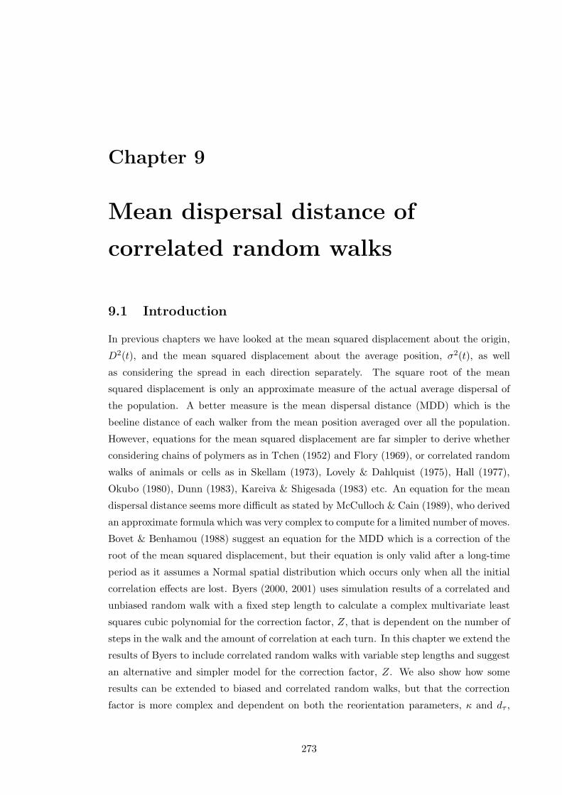
Chapter 9
Mean dispersal distance of
correlated random walks
9.1 Introduction
In previous chapters we have looked at the mean squared displacement about the origin,
D2(t), and the mean squared displacement about the average position, σ2(t), as well
as considering the spread in each direction separately. The square root of the mean
squared displacement is only an approximate measure of the actual average dispersal of
the population. A better measure is the mean dispersal distance (MDD) which is the
beeline distance of each walker from the mean position averaged over all the population.
However, equations for the mean squared displacement are far simpler to derive whether
considering chains of polymers as in Tchen (1952) and Flory (1969), or correlated random
walks of animals or cells as in Skellam (1973), Lovely & Dahlquist (1975), Hall (1977),
Okubo (1980), Dunn (1983), Kareiva & Shigesada (1983) etc. An equation for the mean
dispersal distance seems more difficult as stated by McCulloch & Cain (1989), who derived
an approximate formula which was very complex to compute for a limited number of moves.
Bovet & Benhamou (1988) suggest an equation for the MDD which is a correction of the
root of the mean squared displacement, but their equation is only valid after a long-time
period as it assumes a Normal spatial distribution which occurs only when all the initial
correlation effects are lost. Byers (2000, 2001) uses simulation results of a correlated and
unbiased random walk with a fixed step length to calculate a complex multivariate least
squares cubic polynomial for the correction factor, Z, that is dependent on the number of
steps in the walk and the amount of correlation at each turn. In this chapter we extend the
results of Byers to include correlated random walks with variable step lengths and suggest
an alternative and simpler model for the correction factor, Z. We also show how some
results can be extended to biased and correlated random walks, but that the correction
factor is more complex and dependent on both the reorientation parameters, κ and dτ ,
273

CHAPTER 9: Mean dispersal distance of correlated random walks 274
and time t. Using simulations to find the correction factor for biased random walks with
different reorientation models and reorientation parameters, it is possible to gain more
information about the long-time spatial distribution of the population.
9.2 The mean squared displacement
The standard measure of dispersal is the mean squared displacement. As we have seen
previously, the dispersal (or spread) about the mean position is defined as
σ2(t) =
∫
R2
∫ π
−π‖x − H(t)‖2 p(x, t) dθdx. (9.1)
In an unbiased random walk H(t) = (0, 0) and the spread about the mean position is the
same as the spread about the origin. In Chapter 3 we showed how to derive an equation
for σ2(t) for an unbiased random walk and this is given in (3.43).
9.2.1 Comparing the mean squared displacement for unbiased discrete
random walks and velocity jump processes
Kareiva & Shigesada (1983) derived an equation for the mean squared displacement for a
correlated random walk with a discrete number of time steps n and a symmetric turning
angle distribution g(θ), see (1.75). We can relate their discrete random walk to our
continuous velocity jump process by assuming that n = λt, so that the number of discrete
turns is just the product of the turning frequency and the total time. We now assume
that g(θ) in their model is the same as our von Mises reorientation distribution with no
bias (see (4.9) and (5.2)). The turning frequency in our velocity jump process is governed
by a Poisson process with parameter λ. The time between events in a Poisson process is
exponentially distributed with mean 1/λ and variance 1/λ2. Thus, for our velocity jump
process we have E(l) = sλ , Var(l) = s2
λ2 and E(l2) = 2s2
λ2 . With these results (1.75) becomes
E(R2t ) =
2s2
λ0
(
t− 1
λ0(c− cλt+1)
)
, (9.2)
where c = I1(κ)/I0(κ), and λ0 = λ(1 − c).
For an unbiased random walk, the velocity jump process model gives a solution for the
mean squared displacement, see (3.43). In the absence of bias we have
σ2 =2s2
λ0
(
t− 1
λ0(1 − eλ0t)
)
, (9.3)
where λ0 = λ(1 − c) and c = I1(κ)/I0(κ).
Since 0 < c < 1, the long-time limits of (9.2) and (9.3) are given by
E(R2t )∞ =
2s2
λ0
(
t− c
λ0
)
, (9.4)
and σ2(t)∞ =2s2
λ0
(
t− 1
λ0
)
. (9.5)

CHAPTER 9: Mean dispersal distance of correlated random walks 275
Thus the equations for spread from the velocity jump process model and the model of
Kareiva and Shigesada are very similar with only a slight difference in the constant term,
and the two solutions have the same long-time limiting behaviour.
9.2.2 Mean squared displacement for variable and fixed step lengths
It is worth mentioning that (1.75) highlights the difference between the mean squared
displacement of a random walk with a fixed step length l, so that E(l)2 = E(l2) = l2, and
a random walk with a variable step length with a given mean. An example is the Poisson
process time step in our velocity jump model where our mean step length is l = s/λ and
E(l)2 = (s/λ)2 and E(l2) = 2s2/λ2.
For example, in a random walk with a fixed step length l, E(l)2 = E(l2) = l2, and if we
assume that n = λt and l = s/λ, (1.75) reduces to
E(R2t ) =
s2t(1 − c2) − 2s2c(1 − cλt)
λ20
, (9.6)
where λ0 = λ(1 − c).
From (9.3), a random walk with a step length that is exponentially distributed due to a
Poisson process with parameter λ, has E(l)2 = l2 and E(l2) = 2l2, and if we assume that
n = λt and l = s/λ, (1.75) reduces to
E(R2t ) =
2s2t(1 − c) − 2s2c(1 − cλt)
λ20
. (9.7)
It is immediately clear that for c < 1 the mean squared displacement for the random walk
with the variable step length (9.7), is always larger than the mean squared displacement
for the random walk with the fixed step length (9.6), even though both have the same
mean step length. As c → 0 the former becomes almost twice as large. The variability
of the step length has an important effect on the expected mean square displacement.
This suggests that it is not sensible to model the movement of animals or micro-organisms
with fixed step lengths, if there is likely to be variability in the actual step length used in
the original random walk and one wants to predict information about the mean squared
displacement.
9.3 The mean dispersal distance of unbiased random walks
The mean squared displacement is not always a useful statistic as it is much larger than
the mean dispersal distance (MDD), around which the population will be distributed
(Byers (2001)). Using the notation of the previous chapters, the mean dispersal distance,
MDD(t), is defined as
MDD(t) =
∫
R2
∫ π
−π‖x − H(t)‖ p(x, t) dθdx. (9.8)

CHAPTER 9: Mean dispersal distance of correlated random walks 276
It is not possible to derive a differential equation for MDD(t) for a velocity jump process
as we did for σ2(t) in Chapters 3, 4 and 5. However, equations have been found for
MDD(n), the mean dispersal distance after n steps in a discrete random walk.
9.3.1 Calculating the mean dispersal distance from the mean squared
displacement in a discrete random walk
Using a similar equation for the mean squared displacement given in (1.68), Bovet &
Benhamou (1988) derived an equation for the mean dispersal distance, MDD(n), after a
large number of steps, n. Similar equations to (1.68) have also been used by Flory (1969),
Skellam (1973), Lovely & Dahlquist (1975), Hall (1977), Okubo (1980), Dunn (1983) etc.
when modelling correlated and unbiased random walks.
Assuming a fixed step length l, and a von Mises distribution for the turning angle so that
c = I1(κ)/I0(κ), (1.68) gives
E(R2n) = l2
1 + c
1 − cn− l2
2c(1 − cn)
(1 − c)2. (9.9)
(9.9) has the same limiting behaviour as the equation of Kareiva & Shigesada (1.75) with
a fixed time step for which E(l)2 = E(l2) = l2, see also (9.6). As n becomes large, cn
becomes small since c < 1, and the second term on the right hand side of the above
becomes negligible. The long-time solution is then
E(R2n) ∼ l2
1 + c
1 − cn. (9.10)
Bovet & Benhamou used the following argument to calculate an equation for the mean
dispersal distance MDD(n). Splitting R2n into components gives
R2n = X2
n + Y 2n .
Tchen (1952) showed that when n is large, the two components Xn and Yn are normally
distributed and statistically independent. In a correlated but unbiased random walk there
is no preferential orientation in space and
E(Xn) = E(Yn) = 0, s.d.(Xn) = s.d.(Yn) = δ,
where s.d. represents standard deviation. From this it follows that
E(X2n) = E(Y 2
n ) = δ2,
and therefore
E(R2n) = E(X2
n) + E(Y 2n ) = 2δ2,
or
δ =
√
E(R2n)
2.

CHAPTER 9: Mean dispersal distance of correlated random walks 277
Now let D be the beeline distance from the origin , and let u = Xn/δ and v = Yn/δ, so that
u and v are two independent random variables distributed according to the normal law
N(0, 1). The variable d = D/δ =√u2 + v2 is thus a random variable distributed according
to the χ law with two degrees of freedom. From Evans et al. (2000), the expected value
of a χ law is given by
E(z) =
√2Γ(1
2(µ+ 1))
Γ(µ/2), (9.11)
where µ is number of degrees of freedom. For two dimensions, µ = 2, and we have
E(d) =
√
π
2
and
E(D) = δE(d) =
√
E(R2n)π
4. (9.12)
Thus if E(D) = MDD(n), we can write
MDD(n) =
√
π
4
√
E(R2n), (9.13)
and substituting for (9.10) gives the equation already seen in (1.78):
MDD(n) = l
√
0.79(1 + c)
(1 − c)n. (9.14)
The equation in (9.14) is only valid for large n, as we have only used the long-time limiting
solution for R2n given in (9.10), and because Tchen’s result that the distribution of Xn and
Yn are normally distributed only holds for n large enough so that all correlation effects
have been lost and the spread appears diffusive.
9.3.2 A better model for MDD(n)
The equation derived in the previous section for MDD(n), (9.14), is only valid for large n.
For smaller n the assumption that the spatial distribution is Normal breaks down. Recall
(1.43), the equation for the mean squared displacement of the 1-d telegraph equation:
< x2(t) >=v2
λ
(
t− 1
2λ(1 − e−2λt)
)
. (9.15)
λ is the probability of reversing direction, and thus governs the correlation — if λ is
small the walk is highly correlated. For small λ and small t, < x2(t) >∼ v2t2, which is
characteristic of a wave propagation process, and for large t, < x2(t) >∼ v2t/λ, which is
characteristic of a diffusion process with diffusion coefficient D = s2/2λ.
9.3.2.1 The spread of a two-dimensional correlated random walk
We might expect a similar result to (9.15) in two dimensions — if the random walk is
highly correlated, the initial behaviour will be to spread out linearly from the origin with

CHAPTER 9: Mean dispersal distance of correlated random walks 278
few turns, similar to a wave propagating outwards. As t increases the walk will start to
lose the initial correlation effects and the population spread will become diffusive. If the
walk is not highly correlated we would expect the behaviour to become diffusive more
quickly. This predicted behaviour can be clearly seen in Figure 9.1, for correlated random
walks with κ = 1 (low correlation) and κ = 50 (very high correlation) after a short time.
(a) κ = 1. (b) κ = 50.
Figure 9.1: Plots of the spread of a population of 500 walkers after t = 100, moving as
an unbiased and correlated velocity jump process with (a) κ = 1, (b) κ = 50. The dotted
circle shows the maximum possible displacement at t = 100.
At t = 100 the highly correlated random walk is still spreading out linearly with time
and the spatial distribution is definitely not Normal. After the same time period, the
walk with low correlation appears to be spreading diffusively and the spatial distribution
appears Normal.
This illustrates that the equation of Bovet & Benhamou for the mean dispersal distance,
(9.14), is likely to be valid for smaller n if there is low correlation, but if the walk is highly
correlated, (9.14) will only be valid for very large n.
9.3.2.2 Correction factor method
Byers (2001) compares the equation of Bovet & Benhamou for MDD(n), (9.14), to a
corrected form of the equation of Kareiva & Shigesada (1983):
MDD(n) = Z√
E(R2n), (9.16)
where Z is a correction factor dependent on the number of steps, n, and the degree of
correlation, c, and E(R2n) is calculated from (1.75). The correction factor is needed as
the mean dispersal distance can differ from the root of the mean squared displacement
by as much as 12%. Byers simulated simple random walks with a fixed step length for
various degrees of correlation (giving a range of values of c) and various numbers of steps

CHAPTER 9: Mean dispersal distance of correlated random walks 279
n. Byers fitted a complicated multivariate least squares polynomial to the simulation data
to find the correction factor Z. This was a reasonable fit over only a limited range so five
constraints were also needed. The main result was that 0.89 ≤ Z ≤ 1, with a higher value
of Z for smaller numbers of steps n and higher correlation (c ≈ 1). Byers then shows how
the correction factor equation (9.16) is a better fit to simulation data then the equation of
Bovet & Benhamou, (9.14), for small numbers of steps and high correlation. This seems
obvious as Bovet & Benhamou made it clear that their equation was only a long-time
limiting solution and one would not expect it to be valid if the spatial distribution is not
Normal (which corresponds to small numbers of steps n, and/or high correlation c).
The result obtained by Byers (2001), that the correction factor lies in the range 0.89 ≤Z ≤ 1, is not surprising when one considers the equation of Bovet & Benhamou, (9.14)
and the results in 9.3.2.1. In a correlated random walk, the long-time spatial distribution
will become Normal as n increases (Tchen, 1952), where highly correlated walks will take
a larger number of steps to have a Normal distribution when compared to walks with low
correlation. Bovet & Benhamou show that if the spatial distribution is Normal, then the
ratio between MDD(n) and√
E(R2n) is given by
√
π/4 ≈ 0.89. If the spatial distribution
is similar to a linear spread in time (as in Figure 9.1(b)), then we would expect the ratio
between MDD(n) and√
E(R2n) to be close to 1. If the number of steps is very small then
we also expect the ratio between MDD(n) and√
E(R2n) to be close to 1 (and exactly
equal to 1 for n ≤ 1).
9.3.3 The mean dispersal distance of an unbiased velocity jump process
with a variable time step
We have shown that our equation for σ2(t), (9.3), has the same behaviour as the equation
derived for the mean squared displacement by Kareiva and Shigesada (9.2), when we
assume that n = λt. From (9.13) and the results of Byers, we suggest the following
equation for the mean dispersal distance of an unbiased velocity jump process with a
variable time step:
MDD(t) = Z(c, t)√
σ2(t), (9.17)
where the correction factor Z(c, t) will be dependent on the amount of correlation, c, and
the time, t. In a highly correlated unbiased random walk we would expect Z(c, t) →√
π/4
slowly as t increases, while in a walk with low correlation Z(c, t) →√
π/4 more quickly as
t increases. As long as the walk is unbiased and c < 1, the long-time spatial distribution
will always be Normal and we will always have Z(c,∞) =√
π/4.
The multivariate least squares polynomial fitted by Byers is complicated, has a limited
range, and is calculated from simulation data from a random walk with a fixed step length.
Taking into account the comments on how we expect Z(c, t) to behave, we suggest the

CHAPTER 9: Mean dispersal distance of correlated random walks 280
following simple model for the correction factor
Z(c, t) =
√
π
4+
(
1 −√
π
4
)
exp (−a(1 − c)t) , (9.18)
where a is a constant to be determined and c = I1(κ)/I0(κ). The equation in (9.18) is a
simple decaying function that behaves in the manner described previously, i.e. Z(c, 0) = 1
and Z(c, t) →√
π/4 as t→ ∞, with a slower decrease in Z(c, t) for larger values of c < 1.
9.3.3.1 Estimating Z(c, t)
The equation in (9.18) was fitted against simulation data for a range of values of c and t
to see if the model is reasonable and to find an estimate for the constant a. The simulated
decrease in Z(c, t) does appear to be an exponential decay and our simple model seems
reasonable. The best fit to simulated data was given when a = 16 , although we cannot
justify why it should be this value exactly. Plots comparing the simulated results for Z(c, t)
to the expected values from (9.18) with a = 16 are shown in Figure 9.2 for 0 ≤ t ≤ 500 and
four values of κ.
Allowing for simulation noise, there is a reasonable match between the expected and
simulated values of Z(c, t) as shown in Figure 9.2. The decrease in the simulated Z(c, t)
appears to be exponential and in all the plots Z(c, t) → 0.89 as t increases.
9.3.3.2 Comparing the equation for MDD(t) to simulated random walks
Now that we have a reasonable model for Z(c, t) we can compare the equation for the
mean dispersal distance, MDD(t), given in (9.17) to simulated random walks and also to
other equations in the literature.
In Figure 9.3 we compare our equation for MDD(t) from (9.17) and using the correction
factor in (9.18) with a = 16 , to two other equations for the mean dispersal distance in
the literature — a correction of (9.2) from Kareiva & Shigesada using (9.18) a = 16 , and
the equation of Bovet & Benhamou, (9.14). In Figure 9.4 we demonstrate how our time
dependent correction factor (9.18) with a = 16 , results in a much better estimate for the
mean dispersal distance for highly correlated random walks (large κ) than simply using
the constant long-time limiting value of (9.18).
Figure 9.3 shows two plots of MDD(t) v t for 0 ≤ t ≤ 100. In each plot, we have compared
simulation data with i) the equation for MDD(t) from (9.17) using σ2(t) from (9.3) and
Z(c, t) from (9.18), ii) the equation for MDD(t) from (9.17) using Kareiva & Shigesada’s
equation for R2t , (9.2), in place of σ2(t) and Z(c, t) from (9.18), iii) Bovet & Benahmou’s
equation for MDD(n) from (9.14), using n = λt.
From Figure 9.3 it is hard to distinguish between our equation and the equation of Kareiva
& Shigesada, and both are a very good fit to simulation results. From Figure 9.3(a), for
κ = 1 the equation of Bovet & Benhamou underestimates both the simulated results and
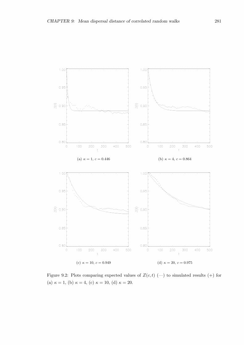
CHAPTER 9: Mean dispersal distance of correlated random walks 281
(a) κ = 1, c = 0.446 (b) κ = 4, c = 0.864
(c) κ = 10, c = 0.949 (d) κ = 20, c = 0.975
Figure 9.2: Plots comparing expected values of Z(c, t) (—) to simulated results (+) for
(a) κ = 1, (b) κ = 4, (c) κ = 10, (d) κ = 20.

CHAPTER 9: Mean dispersal distance of correlated random walks 282
(a) MDD(t) with κ = 1. (b) MDD(t) with κ = 20.
Figure 9.3: Plots of MDD(t) v t for the velocity jump process model (—), Kareiva &
Shigesada’s model (· · ·), Bovet & Benhamou’s model (- -), and simulation results (+).
the results expected from the other two equations. This is because of the point made
in Section 9.2.2 — the equation of Bovet & Benhamou does not take into account the
variable step length that is present. From Figure 9.3(b), for κ = 20 the equation of Bovet
& Benhamou overestimates both the simulated results and the results expected from the
other two equations. This is because the equation of Bovet & Benhamou is only valid
as the long-time limiting solution when the spatial distribution has settled down and is
Normal. A highly correlated random walk (κ = 20) will take a longer time before Bovet &
Benhamou’s equation is valid. If we look at a longer time period (not shown) the equation
of Bovet & Benhamou starts to underestimate the simulated results because of the point
made above about the variable step length.
Figure 9.4 shows plots comparing the results of simulated random walks with i) the equa-
tion forMDD(t) from (9.17) using σ2(t) from (9.3) and Z(c, t) from (9.18), ii) the equation
for MDD(t) from (9.17) using σ2(t) from (9.3) and Z(c, t) = 0.89 ∀ c, t, for 0 ≤ t ≤ 200
and four values of κ.
From Figure 9.4 it is clear that, for all values of κ, there is a good match between simulated
results and expected results for the equation for MDD(t) from (9.17) using σ2(t) from
(9.3) and Z(c, t) from (9.18). For small κ there is little difference between using Z(c, t)
from (9.18) and Z = 0.89 — this is because for a walk with low correlation the spatial
distribution very quickly becomes Normal. When κ is large the expected values using
Z = 0.89 underestimate the simulated values and the expected values using Z(c, t) from

CHAPTER 9: Mean dispersal distance of correlated random walks 283
(a) κ = 1 (b) κ = 4
(c) κ = 10 (d) κ = 20
Figure 9.4: Plots of MDD(t) v t for velocity jump process model with Z(c, t) (—), Z =
0.89 (- -), and simulation results (+).

CHAPTER 9: Mean dispersal distance of correlated random walks 284
(9.18) — this is because the walk is highly correlated and the spatial distribution is not
Normal for these values of t.
9.3.4 The mean dispersal distance in each direction for an unbiased
velocity jump process
In Chapters 4 and 5 we considered not only the total spread about the mean position,
σ2(t), but also the spread about the mean position in each direction, σ2x(t) and σ2
y(t). In a
similar manner we can define MDDx(t) and MDDy(t) to be the mean dispersal distance
in the x and y directions respectively. In an unbiased random walk we would expect
MDDx(t) ≈ MDDy(t) as from previous Chapters we know that if the walk is unbiased,
then σ2x(t) = σ2
y(t).
From Section 9.3.1,we might expect a similar relation between the mean dispersal in each
direction and the spread about the mean in each direction as existed for the total spread
and total mean dispersal. In fact from Evans et al. (2000), the expected value of a χ law
is given in (9.11), and if we consider only one direction, µ = 1 and
E(d) =
√
2
π
and
MDDx(t) =
√
2
πσx(t) ≈ 0.798σx(t), (9.19)
MDDy(t) =
√
2
πσy(t) ≈ 0.798σy(t). (9.20)
Simulations confirm these equations as the long-time limiting relations. The behaviour of
Zx(c, t) and Zy(c, t) is similar to that of Z(c, t) — the ratio between the mean dispersal
distance and the root of the mean squared displacement is equal to 1 at t = 0 and tends
to the limiting value of 0.798 as t increases, with a slower decrease in Z(c, t) for a more
correlated random walk (c ≈ 1). The decrease appears exponential as we found with
Z(c, t), but we have not attempted to fit a function to simulation data.
In a biased random walk we known from Chapters 4, 5 and 6 that the spread is greater
in the non-preferred direction (x) so we would expect the mean dispersal distance to be
greater in the x direction also.
9.4 The mean dispersal distance of biased random walks
In a biased random walk it is not as easy to calculate the mean dispersal distance for
two reasons: i) the spread is larger in the non-preferred direction, and ii) the spread is
not normally distributed. Figure 9.5 shows the spread at t = 100 of a population of 500
walkers moving as a velocity jump process with with parameter dτ = 0.1 and (a) κ = 1
and sinusoidal reorientation, (b) κ = 50 and sinusoidal reorientation, (c) κ = 1 and linear
reorientation, (d) κ = 50 and linear reorientation. Similar results are shown in Figure 8.4.

CHAPTER 9: Mean dispersal distance of correlated random walks 285
(a) Sinusoidal, κ = 1. (b) Sinusoidal, κ = 50.
(c) Linear, κ = 1. (d) Linear, κ = 50.
Figure 9.5: Simulated plots of the spread of a population of 500 walkers after t = 100,
moving as a biased and correlated velocity jump process with dτ = 0.1 and (a) sinusoidal
reorientation, κ = 1, (b) sinusoidal reorientation, κ = 50, (c) linear reorientation, κ = 1,
(d) linear reorientation, κ = 50.

CHAPTER 9: Mean dispersal distance of correlated random walks 286
By inspection of the plot in Figure 9.5(a) and (c), the random walks with small correlation
and bias appear to be approximately normally distributed with similar spread about the
mean in each direction. However, the plots in Figures 9.5(b) and (d) clearly show that the
random walks with bias and high correlation have greater average spread in the x direction,
and the distributions in the y direction do not look Normal and appear skewed towards
the preferred direction (with a larger ‘tail’ for the sinusoidal model). The distributions in
the x direction do appear to be approximately Normal.
9.4.1 The limiting value of the correction factor
From the theoretical and simulated results in Chapters 4, 5, 6 and 8, we know that for
a fixed value of dτ , σ2x(t) → 0 and σ2
y(t) → 0 as κ → ∞, but for a particular value of κ,
σ2x(t) > σ2
y(t).
Now, suppose that the mean dispersal distance in each direction is given by
MDDx(t) = Zxσx(t), (9.21)
MDDy(t) = Zyσy(t), (9.22)
where Zx and Zy are correction factors. In an unbiased random walk we expect Zx, Zy →0.798 as t increases. By definition, we have σ2(t) = σ2
x(t) + σ2y(t) and MDD(t) = Zσ(t),
and combining these and (9.21) and (9.22) gives
Z =MDD(t)
√
MDD2x(t)
Z2x
+MDD2
y(t)
Z2y
. (9.23)
If the walk is weakly biased and correlated then as t → ∞ we will have σ2x(t) ≈ σ2
y(t)
and we would expect Z → 0.89 as in the unbiased random walk. However, if the walk is
highly correlated and biased and σ2x(t) ≫ σ2
y(t) and σ2y(t) ≈ 0, then MDD ≈MDDx and
MDDy ≈ 0. If this is the case then from (9.23), we would expect Z ≈ Zx as t→ ∞.
9.4.2 Simulated behaviour of the limiting value of the correction factor
We have completed simulations of 1000 random walkers, looking at the value of the correc-
tion factor Z(κ, dτ , t) for various values of κ and dτ . In general, the correction factor is 1
when t = 0 and then tends to some limiting value Z(κ, dτ ,∞), but we have not attempted
to fit a decaying exponential function as in the previous section. Simulations were run
up to t = 1000, which gives a good estimate of the long-time limiting behaviour even for
large κ. Figure 9.6 show how the correction factors Z(κ, dτ , 1000), Zx(κ, dτ , 1000) and
Zy(κ, dτ , 1000) change as κ increase from 0 to 50, for dτ = 0.1, 0.5 and 1, and sinusoidal
and linear reorientation.
Allowing for simulation noise, Figures 9.6(a) and (b) show the behaviour that we pre-
dicted. For small κ, Z(κ, dτ , 1000) ≈ 0.89 which suggests that the spatial distribution

CHAPTER 9: Mean dispersal distance of correlated random walks 287
(a) Sinusoidal Z(κ, dτ , 1000) (b) Linear Z(κ, dτ , 1000)
(c) Sinusoidal Zx(κ, dτ , 1000) (d) Linear Zx(κ, dτ , 1000)
(e) Sinusoidal Zy(κ, dτ , 1000) (f) Linear Zy(κ, dτ , 1000)
Figure 9.6: Plots of values of Z(κ, dτ , t), Zx(κ, dτ , t), and Zy(κ, dτ , t) as a function of κ at
t = 1000 from numerical simulations of sinusoidal and linear reorientation with dτ = 0.1
(- -), dτ = 0.5 (· · ·), and dτ = 1 (- · -). The solid lines (—) correspond to Z = 0.798 or
Z = 0.89 respectively, the expected values if the distribution is Normal.

CHAPTER 9: Mean dispersal distance of correlated random walks 288
could be Normal. As κ increases, we start to get MDDx ≫MDDy and Z(κ, dτ , 1000) →Zx(κ, dτ , 1000) ≈ 0.798 as suggested in (9.23). As κ increases, the correction factor de-
creases faster for the larger values of dτ — this is because as κ increases, the spread in the
y direction decreases faster when dτ is larger, as observed in Chapters 4, 5, 6, and 8.
The plots in Figures 9.6(c) and (d), show similar behaviour allowing for simulation noise.
The correction factor for the mean dispersal distance in the non-preferred direction,
Zx(κ, dτ , 1000) appears to be approximately equal to 0.798 for all values of κ in the
simulation. Recall that if the spatial distribution in the x direction is normal then
Zx(κ, dτ ,∞) = 0.798. From the simulation results, we cannot say that the spatial distri-
bution in the x direction is Normal, but we do not have evidence to reject the statement
either. Statistical tests could be used to confirm this result or calculate confidence limits,
but we have not attempted to do this.
The plots in Figure 9.6(f) shows similar behaviour to Figures 9.6(c) and (d) allowing for
simulation noise. We cannot reject the possibility that the spread in the y direction for the
linear model is Normal. However, with the sinusoidal model, the plots in Figure 9.6(e) show
that the correction factor, Zy(κ, dτ , 1000) decreases as κ increases, with the largest decrease
for the larger values of dτ . It appears that the spatial distribution in the y direction for
the sinusoidal reorientation model is not Normal, since Zy(κ, dτ , 1000) 6= 0.798. Recall
the plot of the spatial distribution in Figure 9.5 (b) which suggested a spatial distribution
in the y direction, skewed in the positive y direction with a long tail. In such a spatial
distribution, the mean squared displacement is likely to be a larger relative size than the
mean dispersal distance when compared to a Normal distribution, and hence the correction
factor will be smaller.
Recall that as κ→ ∞, the long-time solutions for the mean dispersal distance will behave
like MDDy(t) → 0 and MDDx(t) ≫ MDDy(t), so that MDDx(t) ≈ MDD(t). This
explains why the plots of Z(κ, dτ , 1000) in Figure 9.6(b) decrease as κ increases, even
though the plots of Zx(κ, dτ , 1000) and Zy(κ, dτ , 1000) both appear to be ≈ 0.798 for all
values of κ.
9.5 Conclusions
In this chapter we have extended the correction factor method of Bovet & Benhamou
(1988) and Byers (2000, 2001), to calculate an equation for the mean dispersal distance
of a correlated and unbiased velocity jump process that is valid for all time. In general, it
is not possible to easily extend the model to include biased random walks as the spatial
distribution does not seem to be Normal. However, by looking at the correction factors
Z(κ, dτ ,∞), Zx(κ, dτ ,∞) and Zy(κ, dτ ,∞) it is possible to gain some information about
the actual spatial distribution in each direction of simulated random walks.
The main results of this chapter are summarised below:

CHAPTER 9: Mean dispersal distance of correlated random walks 289
• The mean squared displacement (MSD) of an unbiased and correlated velocity jump
process is equivalent to the MSD of an unbiased and correlated discrete random
walk, if we assume that the number of steps is given by n = λt.
• An unbiased and correlated random walk with a variable step length can have an
MSD as much as twice as large as an unbiased and correlated random walk with a
fixed step length, given that both walks have the same mean step length, E(l) = l.
• The mean dispersal distance (MDD) of a correlated and unbiased random walk can
be calculated from the square root of the MSD and a correction factor. If the number
of steps, n is large enough so that all initial correlation effects have been lost, then
the population spread is Normally distributed and the correction factor is given by
Z ≈ 0.89. If n is small or the walk is highly correlated, then the population spread
is not Normally distributed and the correction factor lies in the range 0.89 ≤ Z ≤ 1.
• The multivariate least squares polynomial used by Byers (2001) to approximate
Z(c, t) is complicated and limited by constraints. A simple exponential decay model
for Z(c, t) fits simulated data very well for an unbiased and correlated velocity jump
process with a variable step length.
• In a biased and correlated random walk the MSD and MDD are not equal in each
direction as they are in an unbiased walk. If bias is present then MDDx(t) >
MDDy(t), where y is the preferred direction. The spread in the preferred direction
is not normally distributed in general, but the spread in the non-preferred direction
could be normally distributed.
• In a biased and correlated random walk the correction factor lies in the range
0.798 < Z(κ, dτ , t) < 1, while the long-time correction factor lies in the range
0.798 ≥ Z(κ, dτ ,∞) ≥ 0.89. Z(κ, dτ ,∞) is smallest for a random walk with the least
spread in the preferred direction (high correlation and bias), and Z(κ, dτ ,∞) ≈ 0.89
for a walk with small bias and correlation as the walk is similar to an unbiased
walk and the spatial distribution is approximately Normal. The correction factor
Z(κ, dτ , t) is dependent on the correlation and the bias parameters, as well as time
— a simple function for Z(κ, dτ , t) has not been found.
• Simulation results suggest that the spatial distribution in the preferred direction
is not Normal for a biased random walk with sinusoidal reorientation and large
values of the reorientation parameters, as the long-time limiting correction factor
Zy(κ, dτ ,∞) 6= 0.798. For small values of reorientation parameters (κ < 5) in the
sinusoidal model, and all values of κ in the linear model, the spatial distribution in the
y direction could be Normal as Zy(κ, dτ ,∞) ≈ 0.798. The spatial distribution in the
x direction for both reorientation models could be Normal as Zx(κ, dτ ,∞) ≈ 0.798.

Chapter 10
Random walks to a barrier and
the recruitment of fish larvae
10.1 Introduction
In this chapter the random walk models developed in previous chapters are used to inves-
tigate the probability of surviving to reach an absorbing barrier, given that we introduce
a simple mortality model. This model is appropriate to the movement and subsequent
recruitment of fish larvae that typically have a very small chance of survival (recruitment
meaning that the immature larvae are considered to become part of the adult population).
Fish larvae foraging in the open sea have been modelled by Pitchford & Brindley (2001)
and Pitchford et al. (2003), and the variability in an individual’s foraging rate is found to
be critical to its survival probability. Deterministic models of reef fish larvae returning and
recruiting to the reef have been studied by Armsworth (2000, 2001), who demonstrates
that the ability of the larvae to orientate to the reef and direct their motion dramatically
increases the chance of survival when compared to passively advected fish larvae.
We consider three basic reef models: a simple ‘infinite’ linear reef, a finite circular reef,
and a finite circular reef with a constant cross-current.
There are two main conclusions to be taken from our results:
i) If there is a very low survival probability then the variability in the system has an
important effect. Deterministic models are likely to underestimate the true survival
probability.
ii) The survival probability for a fish larva attempting to recruit to a reef is highly
sensitive to its sensing and orientating/swimming abilities. Small changes in the
environment can have a critical impact on the survival probability of a typical reef
fish.
Deterministic models are unlikely to be valid if there is a very low survival probability,
290

CHAPTER 10: Random walks to a barrier and the recruitment of fish larvae 291
and in such cases the variability in the environment or in an individual’s motion cannot
be ignored.
10.2 Background to fish larval movement and recruitment
10.2.1 Recruitment of fish larvae in the open sea
Cushing & Horwood (1994) used a deterministic model to predict the survival probability
of fish larvae in the open sea. Alvarez (2000) showed that if stochastic fluctuations are
included in a system where the growth rate is convex (a positive increasing function with
positive second derivative) then the expected population density will be larger. This is
related to Jensen’s inequality: if f(x) is convex and X is a random variable with mean
X then E(f(X)) > f(X), i.e. the average of the function is greater than the function of
the average (Houston & McNamara, 1999). Using this result, Pitchford & Brindley (2001)
showed that the deterministic model of Cushing & Horwood (1994) will underestimate the
survival probability — the variability in the system is important. More recently, Pitchford
et al. (2003) show that it is not necessarily the fact that the growth rate is convex that is
important, but that it is stochastic and includes an amount of variability. They compare
a deterministic model with a fixed constant growth rate to a stochastic model with the
same fixed constant growth rate plus some white noise. By modelling the weight of the
larvae as a random walk with an absorbing barrier they show that the survival probability
for the stochastic model is always larger than the survival probability for the deterministic
model. The greatest difference between the two models occurs with a large death rate,
large variance and small growth rate.
10.2.2 Recruitment of reef fish larvae
Most reef fishes have a dispersing larval stage which is thought to provide the larvae a
greater chance of avoiding reef predators (Bonhomme & Planes, 2000). This dispersing
stage ends when the larvae leave the pelagic environment and recruit into adult reef
populations. The supply rate of larvae to reefs for recruitment is believed to be a critical
determinant of the structure of reef fish populations (Doherty & Williams, 1988), and the
importance of considering supply rates is acknowledged by those managing reef fisheries
and other industries exploiting these populations, see for example Done et al. (1997).
The dispersal paths of pelagic larvae are determined by local advection in the hydrody-
namic regime around reefs, and initial models assumed that fish larvae were passive during
the dispersal and recruitment process (Dight et al., 1990a,b). Such models predicted a
very small recruitment probability and it was thought that recirculatory features in the lee
of reefs could entrap dispersing larvae, see for example Dight & Black (1991). This idea
led to considerable investment in fine-scale numerical simulations of the hydrodynamic

CHAPTER 10: Random walks to a barrier and the recruitment of fish larvae 292
features of flows around individual reefs (Wolanski & Sarenski, 1997).
However, more recent evidence shows that fish larvae can exhibit directed motion and
are not simply passive (Leis et al., 1996). If swimming of the larvae is included in the
models then the probability of recruitment is increased, see Wolanski et al. (1997). The
most recent theoretical models in the literature that include swimming effects are mainly
deterministic using the assumption that the introduced component of velocity due to
swimming of the larvae aims directly at the target destination, see Wolanski et al. (1997),
Armsworth (2000) and (2001).
We shall show that such deterministic models may be too simple and that the random
variability in the movement of the fish larvae can have a significant effect on the probability
of recruitment.
10.2.3 Theoretical models of fish larvae returning to a reef
Armsworth & Bode (1998) examine the effect of including directed motion in the ensuing
population dynamics and spatial structure. Armsworth (2000) looked at the effects of
directed motion on recruitment by considering 4 cases — strong or weak swimmers, and
current-dependent or current-independent orientation cues. The extent of sensory capa-
bilities of the larvae is critical and the rate of recruitment depends sensitively upon it
for both current-dependent and current-independent orientation cues. Armsworth (2001)
uses a deterministic model to find the most efficient swimming strategy for various reef
environments. To swim efficiently, fish larvae should exploit favourable currents and avoid
unfavourable currents by either directed movement or altering depth of swimming. Such
models do not take into account the variable nature of both the environment and the
swimming of the fish larvae.
10.2.4 Experimental data for fish larvae returning to a reef
There is a large amount of experimental data in the literature mainly from observations
made around the Great Barrier Reef (G.B.R.) in Australia for various coral reef fish species.
Data on current speeds near to reefs
Frith et al. (1986) collected data on current speeds around Lizard Island on the G.B.R.
They found typical current speeds to be 10 − 17 cms−1, but could range from < 5 cms−1
to as much as 60 cms−1.
Data on swimming ability of fish larvae
Leis & Carson-Ewart (1999) made in situ observations of the coral trout (Plectropomus
leopardus) and found that they swam directionally and/or changed depth and were not
simply passive. In general, the swimming speed appeared to be greater moving away from

CHAPTER 10: Random walks to a barrier and the recruitment of fish larvae 293
reefs. In a further study, Leis & Carson-Ewart (2000) observed the movement of four coral
reef fish species and again found that they swam directionally. The larvae swam deeper
in the open ocean and could detect predators 3–6 m away and could change depth and/or
direction to avoid them. They also make the point that in situ observations of reef fish
larvae are extremely difficult due to the depth and nature of the movement. In addition,
the development of swimming ability in larvae of three reef fish species was studied by
Fisher et al. (2000), and development was considerably faster than expected.
Data on swimming speed of fish larvae
Leis & Carson-Ewart (1997) made in situ observations of swimming speeds of fish larvae
near Lizard Island on the G.B.R. and found an average speed of 20.6 cms−1 which is
considered strong. Stobutzki & Bellwood (1997) measured swimming speed duration of
various fish larvae — some larvae can maintain speeds of 13.5 cms−1 for several days with-
out rest. Leis & Carson-Ewart (1999) measured swimming speeds of 7.2 cms−1 towards
the reef and 17.9 cms−1 away from the reef. Sustained swimming times were measured
by Fisher & Bellwood (2002). Speeds between 4 cms−1 and 16 cms−1 were measured and
the average swimming time for each speed recorded. The smallest speed gave the longest
swimming time and also the largest total distance travelled. Bellwood & Fisher (2001)
measured swimming speed for different developmental stages of larvae. The greatest rel-
ative speed (body lengths per second) was for the smaller larvae, but the critical speed
(when leaving pelagic stage and returning to the reef) was determined by developmental
stage and size.
Data on orientation cues
Leis et al. (1996) observed directed motion relative to the reef from over 1 km away.
The orientation cue was unknown, but the average movement was away from the reef,
although measurements were made in daylight. Plumes of warmer water up to 2 km south
of One Tree Reef on the G.B.R. were observed by Doherty et al. (1996), which may pro-
vide a signal or temperature gradient for fish larvae to orientate to. McCauley & Cato
(1998) documented nocturnal peaks in noise levels on reefs from 15 km away, which was
attributed to adult reef fish calling. Similarly, McCauley & Cato (2000) collected statis-
tics of reef noise and found fish calling either en masse or individually ad nauseum, with
the highest activity at night. One call type was found to have a lunar trend. Nocturnal
orientation in response to sound originating from the reef was also measured by Stobutzki
& Bellwood (1998). A review of possible orientation cues available to fish larvae is pre-
sented by Montgomery et al. (2001). Possible cues that were discussed include an innate
sensing ability that may be some sort of magnetic compass sense, ambient sound from the
reef, chemo-sensory signals at small scales, ocean swell and/or wave direction, and visual

CHAPTER 10: Random walks to a barrier and the recruitment of fish larvae 294
location at small distances. Logistical constraints limit experiments designed to establish
which cues are used at small scales of the order of metres, as discussed by for example,
Sweatman (1988) and Stobutzki & Bellwood (1998).
We use the above data from the literature to estimate realistic values for the swimming
speed, current speed, and reef distance in the subsequent random walk models. The exact
values used are given with each model.
Data on reorientation parameters
There is little data available on the turning and orientating behaviour of fish larvae on
both individual and population levels. In the absence of data, a biased random walk
model is plausible because we have evidence of directed swimming plus random changes of
direction — either intrinsic or due to local fluid velocity and turbulence. We do not have
any data to use to estimate the values of the reorientation parameters, κ and dτ , or the
turning frequency, λ, so in the following models we use values that are ‘typical’ of those
observed in swimming micro-organisms by Hill & Hader (1997).
10.3 The effect of variability on fish larvae recruitment
10.3.1 Model 1: simple reef environment
We initially assume a very simple model for the reef environment so that we can use the
asymptotic results derived in Chapters 4 and 5. We assume our fish larvae move around
the (x, y) plane (where the preferred direction is y = x1, and x = x2 using the notation of
Chapters 4 and 5), with no current or flow effects and no interactions between individuals.
We assume that there exists an infinite linear reef at a distance R from the origin in the
y-direction. Thus, any fish larva reaching the position (x, yR) where yR ≥ R and x can
be any value, is assumed to have recruited successfully. Figure 10.1 illustrates this simple
environment.
This ‘infinite’ reef model is reasonable if we assume that the size of the reef is much greater
than the distance the larvae need to move to recruit, R.
As in the velocity jump process models described in Sections 4.2 and 5.2, we assume
that all the fish larvae start at the origin (0, 0) and the population is initially orientated
uniformly around the unit circle, so that for t = 0 we have E(cos(θ)) = 0. We assume
that each fish moves with a fixed speed s, a fixed turning frequency λ, and turns at each
step using either the sinusoidal or linear models with reorientation parameters κ and dτ .

CHAPTER 10: Random walks to a barrier and the recruitment of fish larvae 295
Figure 10.1: Simple ‘infinite’ reef model.
10.3.2 Deterministic model for population dynamics
For walkers moving with the simple random walk model described in Section 10.3.1 we
have derived in Chapters 4 and 5, asymptotic equations for the average position, H(t), and
the average spread about the mean position in each direction, σ2x(t) and σ2
y(t) respectively,
that are dependent on the parameters s, λ, κ and dτ .
A simple deterministic model is to assume that all the population move with the average
absolute velocity Hy(t)/t = VA(t). With the large time scale involved in this system it is
reasonable to approximate the solutions in (4.93) and (5.93) as being linear for all time so
that
VA = VF , (10.1)
where VF = s(Af1 + Bf1) for the sinusoidal model (see (4.72) and (4.73)), and VF is
determined numerically for the linear model. The equations in (4.93) and (5.93) have
extra terms (decaying in time and constants) due to the assumption that we initially have
an equal spread of directions around the unit circle. However, in general the equation in
(10.1) produces results with a relative error of < 1% when compared to (4.93) and (5.93),
due to the large time scales involved in this model.
From (10.1), the time taken to reach the reef is given by
tR =R
VF. (10.2)
To model the effects of natural death, predation etc., we assume the simplest possible
mortality model — deaths occur as a Poisson process with rate µ. Thus, the probability
that an individual survives to a certain time tR is simply exp(−µtR), and the probability
of surviving to reach the reef is given by
PR(VF , 0) = exp
(
−µRVF
)
, (10.3)

CHAPTER 10: Random walks to a barrier and the recruitment of fish larvae 296
where the notation PR(VF , 0) denotes the probability of reaching the reef for a fish larva
moving with absolute velocity in the y-direction given by VF and with variance per unit
time γ2, where γ = 0 for this deterministic model.
10.3.3 Stochastic model for population dynamics
As in the deterministic model we assume that the average absolute velocity Hy(t)/t can
be approximated by the linear function VF because of the large time scale used. Similarly,
the long-time equations for the spread about the mean position are linear in time (see
Chapters 4, 5 & 6), and it is reasonable to assume that the equations for the spread about
the mean position in each direction, σ2x(t) and σ2
y(t), can be approximated by the linear
functions ς2t and γ2t respectively. To calculate the time at which each walker reaches a
specified position in the y direction, we only consider the mean position in the y direction,
VF t, and the spread in the y direction, γ2t.
From Section 1.1.3, (1.30) gives the stopping time for a population of walkers with an ab-
sorbing barrier at y = R, and whose movement is governed by the drift diffusion equation:
∂g
∂t= −u∂g
∂y+v2
2
∂2g
∂y2y > 0, (10.4)
where g(y, t) is the probability density function (p.d.f.), ut gives the average position and
v2t gives the variance about the average position. In the absence of a barrier, such a
population is normally distributed in space with p.d.f. N(ut, v2t), see Section 1.1.2.
Our velocity jump process models are not the same as random diffusive processes as we
have extensively discussed in previous chapters. The advantage of the diffusion equation
with drift, (10.4), is that it is easily solved with various boundary conditions, including
an absorbing barrier (Grimmett & Stirzaker, 2001), whereas this is not possible with
the velocity jump process as we do not know the underlying spatial distribution. From
Chapter 9, we know that the long-time spatial distribution of the velocity jump process
is approximately Normal if the reorientation parameters are small. To make comparisons
to simulated results, we assume that for small reorientation parameters our velocity jump
process can be approximated by (10.4) with u = VF and v2 = γ2. We do not expect an
exact fit between this model and simulated results as the velocity jump process used in
the simulations is not the same as simple diffusion with drift. We will see later that even
this approximate model that includes stochastic effects is a better fit to simulated results
than the deterministic model in Section 10.3.2.
From Section 1.1.3 and Grimmett & Stirzaker (2001), the p.d.f. for the stopping time, tR,
for a population with movement governed by (10.4) and with a barrier at y = R is given
by
ftR =R
√
2πγ2t3exp
(
−(R− VF t)2
2γ2t
)
, (10.5)

CHAPTER 10: Random walks to a barrier and the recruitment of fish larvae 297
which takes a similar form to the stopping time p.d.f. derived by Pitchford et al. (2003)
when modelling the growth of foraging fish larvae as a Brownian process. To calculate
the probability of survival it is necessary to take into account this distribution of stopping
times rather than just assuming all the fish larvae reach the reef at the same time. The
probability of an individual reaching the reef is given by
PR(VF , γ) =
∫
∞
0ftRe
−µt dt
= exp
[
RVFγ2
(
1 −√
1 +2µγ2
V 2F
)]
, (10.6)
which is again similar to the solution obtained by Pitchford et al. (2003). From Pitchford
et al. (2003), PR(VF , γ) > PR(VF , 0) for any γ > 0 — the variance in the model always
results in a higher survival probability even in this simple model. The relative survival
probability is given by
RSP ≡ PR(VF , γ)
PR(VF , 0)= exp
[
Rµ2γ2
2V 3F
+O
(
Rµ3γ4
V 5F
)]
, (10.7)
and as in Pitchford et al. (2003), the beneficial effects of the variance are felt most strongly
in a high death rate, high spatial spread, low absolute velocity regime. Fish larvae are
certainly susceptible to a very high death rate mainly due to predation. In the open sea, a
typical survival rate is O(1%) (Chambers and Trippel, 1997) while Pitchford & Brindley
(2001) use a death rate per day of ∼ 10%, so we may expect variance in the movement of
the larvae to have an important effect on the survival probability.
10.3.4 Survival probabilities for the simple reef model
From the experimental data in the literature given in Section 10.2.4 a realistic value for the
average speed of fish larvae is 0.1 ms−1, while the distance of the reef can be anything from
a few metres to several kilometres — we shall use a value of R = 200 m for the following
simulations. Estimates for the turning rate λ and reorientation parameters κ and dτ are
not available in the literature so we have chosen values that seem sensible and are not
too extreme, these values being λ = 1/2, κ = 2 and dτ = 0.1. With these parameters,
and using the sinusoidal reorientation model, VF = 0.0114 and γ2 = 0.0640, so that we
have a small absolute velocity. The expected arrival time at the reef for the deterministic
model is given by tR ≈ 17500s (just under 5 hours), while the stochastic model gives a
distribution of arrival times peaked around tR.
To illustrate the main result in Section 10.3.3 (that variance is important and the deter-
ministic model will underestimate the survival probability), we have looked at a range of
values for the death rate µ, between 0.0001 s−1 and 0.0004 s−1. This death rate may seem
quite low compared to the death rates discussed previously, but considering the large time
taken to reach the reef it is actually quite high and the probability of survival will be seen
to be O(5%).

CHAPTER 10: Random walks to a barrier and the recruitment of fish larvae 298
Simulations were completed with 100,000 walkers all moving with the random walk model
described in Section 10.3.1, and subject to a Poisson process death rate with values of the
parameter µ between 0.0001 s−1 and 0.0004 s−1. Figure 10.2(a) and (b) show the survival
probability against µ for the deterministic model (10.3), the stochastic model (10.6) and
the simulation results PR(sim), with (a) 0.0001 ≤ µ ≤ 0.0002, and (b) 0.0002 ≤ µ ≤0.0004. We have displayed two separate plots to highlight the relative difference between
the deterministic, stochastic and simulated results at very small survival probabilities.
(a) PR(VF , γ) v µ (b) PR(VF , γ) v µ
Figure 10.2: Plots showing (a) survival probability PR(VF , γ) against death rate for (a)
0.0001 ≤ µ ≤ 0.0002, and (b) 0.0002 ≤ µ ≤ 0.0004. Legend: deterministic model (—),
stochastic model (- -), simulation model (+).
From Figures 10.2(a) and (b), one can see that, although the simulation data is fairly
noisy, the simulated survival probability, PR(sim), is always larger than the deterministic
survival probability, PR(VF , 0). Allowing for simulation noise, there is a reasonable fit
between PR(sim) and PR(VF , γ), the stochastic survival probability, even though PR(VF , γ)
is only a diffusion approximation to the velocity jump process used in the simulations. The
behaviour in Figures 10.2(a) and (b) is very similar to that shown in Figure 1 of Pitchford
et al. (2003).
Figure 10.3 shows the relative survival probability for the theoretical and simulated models,
(see (10.7)), when compared to the deterministic survival probability, PR(VF , 0).
Although Figure 10.3 shows a lot of simulation noise, the general behaviour is clear — as
the death rate µ increases (and consequently PR(VF , 0) decreases), the relative survival
probabilities of both the simulated and stochastic models become larger when compared
to the deterministic model.

CHAPTER 10: Random walks to a barrier and the recruitment of fish larvae 299
Figure 10.3: Plots of relative survival probability RSP against PR(VF , 0) from theoretical
(—) and simulation (+) results.
The simulations were completed using the sinusoidal reorientation model — results using
the linear reorientation model are qualitatively similar, although the linear model gives a
higher survival probability with the same values for the reorientation parameters (recall
that the linear model always gives a higher absolute displacement for the same parameter
values). Similarly, if reorientation parameters that produce a larger absolute displacement
are used then the survival probability is larger and the relative survival probability is
smaller, but the qualitative results are similar. Similar results might also be expected if
the death rate is made smaller but the distance to the reef is made larger.
When dealing with systems with very small survival probabilities, such as this simple
example of fish larvae attempting to recruit to a reef or the model of Pitchford et al. (2003)
with foraging fish, it seems clear that the variability in the model cannot be discounted
as deterministic models will underestimate the true survival probability.
From the literature (Leis et al. (1996), Stobutzki & Bellwood (1988) etc.), it seems likely
that fish larvae move away from the reef during the day (possibly to maintain their position
in the open water), and attempt to reach the reef at night. If we assume that a fish larva
can only recruit during the hours of darkness, then there will be a 6-10 hour time limit for
recruitment to the reef to take place. Any fish that are still in the open water after this time
limit are assumed to die. To model this in our theory and simulations we can introduce
a ‘cut-off’ time, T , and assume that PR(t > T ) = 0. This has important implications —
if our deterministic model predicts that R/VF = tR > T then we now have an expected
survival probability of zero, P (VF , 0) = 0, and the deterministic model is useless. The

CHAPTER 10: Random walks to a barrier and the recruitment of fish larvae 300
stochastic model could still be used although we now have different boundary conditions
and the probability of survival will be smaller.
10.4 Optimal swimming behaviour for fish larvae attempt-
ing to recruit to a reef
In the previous section we noted that the survival probability will increase if the expected
average displacement towards the reef increases. In this section we will investigate the
effect of changing the reorientation parameters on the survival probability. From Section
4.2.4, we consider the parameter dτ as the ‘sensing’ ability and the parameter κ as the
‘orientating/swimming’ ability (the ability to overcome the inherent randomness in the
environment). We have seen in Sections 8.2.1 and 8.2.2 that the optimal values of the
parameters (to produce the maximum average displacement) are κ → ∞ and dτ = 1
(linear model) and 1 ≤ dτ ≤ π2 (sinusoidal model), and we might expect the largest
survival probabilities for these optimal parameter values.
We have looked at a simple infinite reef model in the previous section and the results are
not repeated here. Similarly to the simulation results presented in Chapter 8, the models
and parameter values considered in this section do not fit for the asymptotic solutions
from Chapters 4 and 5, and so we only look at simulation results.
10.4.1 Model 2: simple circular reef model
We assume exactly the same environment as in Section 10.3.1, except that instead of an
infinite linear reef we now have a small circular reef of radius r, centred at the point (0, C),
see Figure 10.4. We also introduce a cut-off time, T , after which any fish larvae that have
not reached the reef are assumed to be dead.
In a similar manner to the model described in Section 8.4, the fish larvae always attempt
to reorientate to the centre of the reef, so that the preferred direction is not constant but
dependent on the spatial position.
Simulations of 1000 fish larvae moving towards a circular reef have been completed for the
sinusoidal and linear reorientation models for various values of the reorientation parameters
κ and dτ . In all the simulations we use the following parameter values: the cut-off time
T = 10 hours (36, 000 s), the speed s = 0.1 ms−1, the turning frequency λ = 0.5 s−1, the
distance to the centre of the reef C = 500 m, the radius of the reef r = 10 m, and the death
rate µ = ln(0.5)/36, 000 s−1, so that the probability of surviving the effects of predation,
natural death etc. for 10 hours is Psurv(10hrs) = 0.5 (at which point any surviving fish
larvae that have not reached the reef are killed off). Up to the cut-off point T , this is a
low death rate compared to the previous section.

CHAPTER 10: Random walks to a barrier and the recruitment of fish larvae 301
Figure 10.4: Simple circular reef model.
With these parameters, the theoretical minimum time to reach the reef is given by tmin =
4900 s, corresponding to moving directly from the origin to the edge of the reef in a straight
line (i.e. VF = s = 0.1). Such models that do not include random fluctuations of the
individual movement have been considered by Armsworth (2000, 2001). The probability
of reaching the reef and surviving in this extreme case is PR(VF = 0.1) = 0.9100. This
gives an expected upper bound for the survival probabilities of the subsequent simulations
that do include the effects of random reorientations in the individual movement.
10.4.1.1 Sinusoidal reorientation
The plots in Figure 10.5 show how the simulated survival probability for reef model 2 with
sinusoidal reorientation changes as (a) κ increases for 4 values of dτ , (b) dτ increases for
4 values of κ.
In Figure 10.5(a) the survival probability PR(dτ , κ) > 0 as long as dτ > 0 and κ is large
enough, while in Figure 10.5(b) PR(dτ , κ) = 0 for κ < 0.4 and all values of dτ , indicating
that the survival probability is likely to be less than 1/1000 for these values.
10.4.1.2 Linear reorientation
The plots in Figure 10.6 show how the simulated survival probability for reef model 2 with
linear reorientation changes as (a) κ increases for 4 values of dτ , (b) dτ increases for 4
values of κ.
As in the sinusoidal model, in Figure 10.6(a) the survival probability PR(dτ , κ) > 0 as long
as dτ > 0 and κ is large enough, while in Figure 10.6(b) PR(dτ , κ) = 0 for κ < 0.4 and
all values of dτ , indicating that the survival probability is likely to be less than 1/1000 for
these values.

CHAPTER 10: Random walks to a barrier and the recruitment of fish larvae 302
(a) PR(dτ , κ) v κ (b) PR(dτ , κ) v dτ
Figure 10.5: Plots showing survival probability PR(dτ , κ) for sinusoidal reorientation and
Model 2 against (a) κ, for dτ = 0.1 (—), dτ = 0.3 (- -), dτ = 0.5 (· · ·), and dτ = 1.0 (- · -);
(b) dτ , for κ = 0.4 (—), κ = 1.0 (- -), κ = 2.0 (· · ·), and κ = 4.0 (- · -).
(a) PR(dτ , κ) v κ (b) PR(dτ , κ) v dτ
Figure 10.6: Plots showing survival probability PR(dτ , κ) for linear reorientation and
Model 2 against (a) κ, for dτ = 0.1 (—), dτ = 0.3 (- -), dτ = 0.5 (· · ·), and dτ = 1.0
(- · -); (b) dτ , for κ = 0.4 (—), κ = 1.0 (- -), κ = 2.0 (· · ·), and κ = 4.0 (- · -).

CHAPTER 10: Random walks to a barrier and the recruitment of fish larvae 303
10.4.1.3 Comments on survival probabilities for Model 2
Figures 10.5(a) and 10.6(a) show similar behaviour — for each value of dτ there is a critical
value of κ, such that for all κ < κcrit, PR(dτ , κ) = 0 in our simulations. Compare these
results to the plots in Figure 8.1 — the highest survival probability corresponds to the
highest average displacement in the preferred direction, as might be expected. However,
the increase in the average displacement in Figure 8.1 is approximately linear with κ for
small κ. The plots in 10.5(a) and 10.6(a) show a sudden jump from a survival probability
close to zero to a survival probability that is close to the theoretical maximum. As κ
increases further the survival probability seems to tend asymptotically to the theoretical
maximum.
Figures 10.5(b) and 10.6(b) also show similar behaviour — there is a sudden jump in the
survival probability for a critical value of dτ . Comparing to the plots in Figure 8.5, the
largest survival probability corresponds to the optimal value of dτ , however the increase
in the average displacement with dτ is a lot smoother and there is no sudden jump as we
see with the survival probability plots. The maximum survival probability seems to be
independent of dτ and critically dependent on κ — even if the sensing ability is optimal
dτ = dopt, if there is too much turbulence or the fish larvae cannot orientate to the preferred
direction very well (small κ) then the survival probability will always be low.
If the reef is further away, or the fish have a slower speed, then the survival probabilities
decrease but the qualitative behaviour is similar and plots are omitted.
It seems that in general, the fish larvae either have a very low (or zero) survival probability
or a reasonably high survival probability with not much middle ground. The values of the
reorientation parameters are critical to determining the survival probability.
It is not unreasonable to think that our fish larvae would evolve to be just good enough
swimmers to give a high survival probability but would not be any better than necessary
(i.e. they would be just at the top of the switch in survival probabilities observed above).
If this were the case, a slight change in the environment would result in a catastrophic
change in survival probability that results in massive decrease in the number of fish larvae
managing to recruit.
10.4.2 Model 3: simple current model
We assume exactly the same environment as in Section 10.4.1, except that we now intro-
duce a cross-current of fixed magnitude U , see Figure 10.7.
A cross-current would have no effect on the simple infinite linear reef model as the current
only increases the x position and fish larvae would still reach the reef at the same time
(albeit at a different point on the reef). However, the cross-current will certainly have an
effect when the fish larvae are trying to reach a small circular reef. It is not of particular

CHAPTER 10: Random walks to a barrier and the recruitment of fish larvae 304
Figure 10.7: Circular reef with a constant current.
interest to look at a current that produces a drift directly towards the reef relative to the
origin of the fish larvae, as this just increases the absolute velocity VF , while a current that
produces a drift away from the reef will decrease the absolute velocity VF , see Armsworth
(2000).
Simulations of 1000 fish larvae moving towards a circular reef with a constant cross-current
have been completed for the sinusoidal and linear reorientation models for various values
of the reorientation parameters κ and dτ . In all the simulations we have used the same
parameter values as in Section 10.4.1, and the current speed U = 0.05 ms−1, which is not
unrealistic when compared to measured current speeds near reefs, see Frith et al. (1986).
With these parameters, the theoretical minimum time to reach the reef is found by
Pythagoras Theorem, where we have a triangle of sides 490 m, 0.05tmin m and hypotenuse
0.1tmin m. Thus, the optimal orientation is to move slightly into the current, so that the
drift takes one to the reef, see Armsworth (2001). Solving this gives tmin = 5658 s. The
probability of reaching the reef and surviving in this case is PR = 0.8968, which gives an
expected upper bound that is only slightly smaller than in Section 10.4.1. It is clear that
by increasing the magnitude of the current U , the minimum time to reach the reef tmin
will increase and consequently the survival probability will decrease. In fact as U → s the
theoretical survival probability tends to zero, PR → 0.
10.4.2.1 Sinusoidal reorientation
The plots in Figure 10.8 show how the simulated survival probability for reef model 3 with
sinusoidal reorientation changes as (a) κ increases for 4 values of dτ , (b) dτ increases for
4 values of κ.

CHAPTER 10: Random walks to a barrier and the recruitment of fish larvae 305
(a) PR(dτ , κ) v κ (b) PR(dτ , κ) v dτ
Figure 10.8: Plots showing survival probability PR(dτ , κ) for sinusoidal reorientation and
Model 3 against (a) κ, for dτ = 0.2 (—), dτ = 0.5 (- -), dτ = 1.0 (· · ·), and dτ = 1.5 (- · -);
(b) dτ , for κ = 1.8 (—), κ = 2.0 (- -), κ = 3.0 (· · ·), and κ = 5.0 (- · -).
In Figure 10.8(a) the survival probability PR(dτ , κ) > 0 as long as dτ > 0.1 and κ is large
enough, while in Figure 10.8(b) PR(dτ , κ) = 0 for κ < 1.8 and all values of dτ . Thus, the
true survival probability is likely to be less than 1/1000 for κ < 1.8, which is larger than
the equivalent value in the non-current model (κ < 0.4). Unlike the non-current model, for
this range of κ values the survival probability is likely to be less than 1/1000 for dτ < 0.2.
10.4.2.2 Linear reorientation
The plots in Figure 10.9 show how the simulated survival probability for reef model 3 with
linear reorientation changes as (a) κ increases for 4 values of dτ , (b) dτ increases for 4
values of κ.
In Figure 10.9(a) the survival probability PR(dτ , κ) > 0 as long as dτ > 0 and κ is large
enough (unlike the sinusoidal model with current for these values of κ), while in Figure
10.9(b) PR(dτ , κ) = 0 for κ < 1.4 and all values of dτ . Thus, the true survival probability
is likely to be less than 1/1000 for κ < 1.4 which is larger than the equivalent value in the
non-current model (κ < 0.4), but smaller than the critical value for the sinusoidal model
with current (κ < 1.8).
10.4.2.3 The effect of the current on the survival probability
The plots in Figure 10.10 show how the simulated survival probability for reef model 3 with
dτ = 0.8 changes as U increases for (a) sinusoidal reorientation, (b) linear reorientation.
As expected, the survival probability tends to zero as the current speed increases, PR → 0
as U → s, but the behaviour is not smooth and features the same sudden jump as discussed

CHAPTER 10: Random walks to a barrier and the recruitment of fish larvae 306
(a) PR(dτ , κ) v κ (b) PR(dτ , κ) v dτ
Figure 10.9: Plots showing survival probability PR(dτ , κ) for linear reorientation and
Model 3 against (a) κ, for dτ = 0.1 (—), dτ = 0.3 (- -), dτ = 0.5 (· · ·), and dτ = 1.0
(- · -); (b) dτ , for κ = 1.4 (—), κ = 2.0 (- -), κ = 3.0 (· · ·), and κ = 5.0 (- · -).
(a) Sinusoidal PR(U, κ) v U (b) Linear PR(U, κ) v U
Figure 10.10: Plots showing survival probability PR(U, κ) v U with dτ = 0.8 for (a)
sinusoidal reorientation and (b) linear reorientation. Legend: κ = 1.0 (—), κ = 2.0 (- -),
κ = 3.0 (· · ·), and κ = 5.0 (- · -).

CHAPTER 10: Random walks to a barrier and the recruitment of fish larvae 307
previously. For fixed reorientation parameters there is a critical current magnitude, such
that U > Ucrit results in a zero survival probability in the simulations. For the same
parameter values, it is clear that the survival probability for the linear model is greater
than that for the sinusoidal model.
10.4.2.4 Comments on survival probabilities for Model 3
The plots in Figures 10.8 and 10.9 show very similar qualitative behaviour to Figures 10.5
and 10.6 and similar conclusions and comments to those made in Section 10.4.1.3 apply.
The survival probabilities have significantly decreased when compared to the results from
Model 2, and the critical values of the reorientation parameters are now larger — the fish
larvae need to be better at sensing and orientating towards the reef because in general the
current is taking them away from it.
For fixed reorientation parameters, the survival probability is also critically dependent on
the current magnitude, U . For small U , the survival probability is close to the upper
bound predicted, with a slow decrease in survival probability as U increases. However,
once U > Ucrit there is a massive drop in the survival probability which becomes close to
zero. If the current is faster than the speed of movement, U > s, then the fish larvae have
zero survival probability in this reef environment.
10.4.3 Further models
It is straightforward to adapt our simulation model to include even more realistic effects
such as spatially dependent parameters as in Sections 8.3.1 and 8.3.2 — it makes sense for
the larvae’s sensing ability (dτ ) to increase as it gets closer to the reef, while an increase
in κ could correspond to the larvae moving away from the turbulent open water and into
the calmer waters near the reef so that we have an inhomogeneous environment.
If we model the sensing ability as spatially dependent it is necessary to consider the
orientation cues to the reef that the larvae use, see Montgomery et al. (2001). If the cue
is sound (McCauley & Cato (1998) and (2000), Stobutzki & Bellwood (1998) etc.), then
although the fluid dynamics and turbulence of the water could effect the dispersal of the
sound wave, it is not unreasonable to model the signal as spreading out in all directions
from the centre of the reef. If the cues are chemical, then currents and turbulence will
have a much more obvious effect on the dispersal of the signal — the orientation cue
will be different depending on whether a larvae is upstream or downstream from the reef
(Armsworth, 2000) It is likely that fish larvae use a number of different orientation cues
at different scales — sound at large distances, and then chemical or even visual cues at
smaller distances, see Montgomery et al. (2001).
We have completed several simulations looking at the spatial dependence of the orienta-
tion cues, and consequently the reorientation parameters κ and dτ . In general, there is

CHAPTER 10: Random walks to a barrier and the recruitment of fish larvae 308
little qualitative difference to the results in Sections 10.4.1 and 10.4.2 and results are not
presented. For example, the survival probability will decrease if dτ is spatially dependent
with a limiting value dopt, when compared to a fixed value of dτ = dopt for all spatial
positions. The overall survival probability is still highly sensitive to the value of κ that is
used.
One extension to the model that may be worth considering is a variable death rate µ
depending on the spatial position and also the depth of the fish larvae (which may require a
three dimensional simulation model). There is evidence that fish larvae can sense predators
and will move away and or change their depth to avoid being eaten, see Leis & Carson-
Ewart (1999). There is also the possibility that fish larvae use the fact that currents
are different magnitudes (and possibly even different directions) at different depths, to
maximise their chances of reaching the reef (Armsworth, 2001).
What seems certain is that passive advection of the fish larvae through pure diffusion or
favourable currents is unlikely to result in a non-zero survival probability. By developing
basic reorientation and swimming abilities a reef fish larva can dramatically increase its
chances of surviving to reach the reef and recruit into the adult population.
10.5 Conclusions
By adding individual-based mortality to the theoretical and simulation random walk mod-
els developed in previous chapters we have shown how they can be applied to a useful
application — the survival probability of pelagic reef fish larvae. We have used data from
the literature to estimate parameter values such as swimming speed and current speed.
There does not appear to be any data in the literature that we can use to estimate our
reorientation parameters, so we have made what we consider sensible estimates.
For a simple ‘infinite’ linear reef environment model with a high death rate we have very
similar results to Pitchford et al. (2003), in that a simple deterministic model (where all
the fish larvae are assumed to have the same absolute velocity) will always underestimate
the survival probability obtained from stochastic models and simulation results. The
variability in the movement of the fish larvae is important when the survival probability
is very low.
More complicated reef environment models have been studied using simulations — it is
possible to introduce a circular reef of fixed size and also a cross-current of constant mag-
nitude. Using these simulation models we have investigated the effect that the individual
sensing ability (dτ parameter) and orientating ability (κ parameter) of the fish larvae has
on the survival probability of a population attempting to recruit. There appears to be
a critical dependence on the reorientation parameters with either a very low (or zero)
survival probability, or a relatively high survival probability and no middle ground. This

CHAPTER 10: Random walks to a barrier and the recruitment of fish larvae 309
may be significant if fish larvae have evolved to be adapted to a particular environment
— if the environment changes and the fish larvae subsequently are less able to sense or
orientate to the reef then there will be huge decrease in the survival probability. Deter-
ministic models such as Armsworth (2000) and (2001) do not predict this high sensitivity
on the swimming abilities of the fish larvae.
More complicated models such as spatially dependent reorientation parameters or diffusive
signals have been considered, but initial simulation results do not show any significantly
different behaviour to the simpler models. Worthwhile extensions may be to investigate
a variable death rate that could account for the fish larvae avoiding predators by moving
away or changing their depth, or a variable current to take into account the fish larvae
altering their depth to find more favourable currents. Both these extensions may be better
suited to three-dimensional simulations.
The main results of this chapter are summarised below:
• Our theoretical and simulation random walk models can be used to model the move-
ment and recruitment of fish larvae returning to reefs.
• In general, deterministic models underestimate the survival probability if there is
variability in the system. The variability will have more effect on the survival prob-
ability if there is a high death rate, a large spatial spread and a small absolute
velocity.
• The survival probability is highly sensitive to the reorientation parameters κ (which
we consider the orientating ability), and dτ (which we consider the sensing ability).
A change in the environment could have produce a large decrease in the survival
probability if the fish larvae can not change their swimming abilities.
• The parameter κ is highly critical to the survival probability even if dτ is optimal
— it is no use being able to sense the direction of the reef perfectly if the fish larvae
cannot orientate to move in that direction.
• More complex reef environment models that we have simulated produce similar re-
sults, but further three dimensional simulations that take into account the depth of
the fish, variable currents, and a variable death rate may be worthwhile if there is a
need to study a particular environment.

Chapter 11
Concluding remarks
11.1 Main results
In this thesis we have extended the method of calculating the moments of the underlying
spatial distribution of a two-dimensional velocity jump process (Othmer et al., 1988) to
include realistic reorientation models as suggested by Hill & Hader (1997), where bias
is introduced by the dependence of the mean turning angle on the absolute angle of the
previous direction of movement. Simple diffusive models based on position jump processes
allow for infinite propagation and cannot take account of the dependence of the mean
turning angle on the previous direction of movement, whereas a velocity jump process
can take this into account as the random walk is in the velocity and not the position.
The main problem encountered with the velocity jump process is that it is not possible
to derive an equation for the underlying spatial distribution in two dimensions, although
in one dimension one can derive the telegraph equation (Goldstein, 1952; Kac, 1974).
Othmer et al. got around this problem by deriving equations for the moments of the
underlying spatial distribution directly. The reorientation models used by Othmer et al.
are somewhat artificial, but do result in a simple closed system of differential equations for
the moments of the underlying spatial distribution. Hill & Hader’s reorientation models
are more realistic and have reorientation parameters (κ and dτ ) that can be directly
measured by simple experiments. However, to arrive at a closed system of differential
equations for the higher order moments using these more realistic reorientation models, it
is necessary to make several assumptions and the final solutions for the required statistics
are asymptotic expansions only valid for small values of the parameter dτ .
Using numerical simulations of velocity jump processes with Hill & Hader’s reorientation
models, we show that the asymptotic solutions are a good fit to simulated data over a
wide range of parameter values, and only start to break down when both reorientation
parameters are large. Using the same simulation model it is also possible to investigate ve-
locity jump processes at parameter values for which the asymptotic solutions are not valid.
We have looked at large reorientation parameters and spatially dependent parameters, as
310

CHAPTER 11: Concluding remarks 311
well as the effect of a changing preferred direction. The same simulation model could be
used to investigate further extensions of the velocity jump process where it may not be
possible to derive theoretical solutions or approximations. Extensions to the model that
would be biologically relevant include variable speed and/or turning frequency, waiting
times between steps, temporally dependent parameters, nonhomogeneity in the environ-
ment, interactions between individual walkers, and allowing movement in three dimensions
rather than restricting the model to two dimensions.
With the same simulation model, we have investigated how valid the method used by Hill
& Hader to calculate the reorientation parameters from observed data is, when the original
random walk is not continuous but a velocity jump process. Their method is valid but
for velocity jump processes with large times between turns it tends to underestimate the
true values of the reorientation parameters. The closer the velocity jump process is to a
continuous random walk, the better the estimates of the reorientation parameters are. If
the sampling length used is too large the method will also underestimate the reorientation
parameters, and comparing simulation results to the results of Hill & Hader suggests that
their sampling length was too large, although their smallest sampling length used was an
experimental constraint.
Various authors have tried to determine the relation between the root of the mean squared
displacement (MSD) and the mean dispersal distance (MDD), either by resolving simula-
tions (Byers, 2000, 2001) or finding a direct analytic relation (Bovet & Benhamou, 1988;
McCulloch & Cain, 1989). We have suggested a model for the correction factor between
the root of the MSD and the MDD for a correlated and unbiased random walk that is
valid for all time. The model is much simpler than previous ones in the literature (Byers,
2000, 2001), but fits simulated data well. With simulations we have studied the MDD of a
biased and correlated random walk, and although we have not found a simple equation for
the correction factor, we have shown for certain cases that the spatial distribution cannot
be Normal, unlike the case with the long-time distribution of an unbiased and correlated
random walk.
Finally, we have demonstrated a direct application of our velocity jump process model
to the directed movement and subsequent recruitment of reef fish larvae. With a simple
reef environment, we use a diffusion approximation of our velocity jump process model
to compare to simulated results, and show that deterministic models underestimate the
survival probability if there is a high death rate. In more complex reef environments, sim-
ulations are used to investigate the optimal swimming behaviour — although the sensing
ability has an effect on the survival probability, it seems to be the swimming and orientat-
ing ability that determines the maximum survival probability. The survival probability is
found to be highly sensitive to critical parameter values, suggesting that in a homogeneous
population, fluctuations in the environment could have a catastrophic effect on the size
of the recruited population. More complex reef models can be simulated, for example by

CHAPTER 11: Concluding remarks 312
adding spatially dependent parameters but this has little effect on the main conclusions
previously made. Realistic effects mentioned in the literature that we have not considered
and that may effect the survival probability include a variable death rate, the effects of
the larvae altering depth, and variable currents and tides. All could be readily modelled
with more sophisticated simulations.
We believe we have presented a fundamental framework for modelling the movement of
animals and micro-organisms using random walks where bias is introduced through the
dependence of the mean turning angle on the previous direction of movement, as observed
in Hill & Hader’s experiments. Modelling the random walk as a velocity jump process with
this realistic reorientation model has its limitations — the asymptotic equations derived
for the spatial statistics of interest are only valid for small reorientation parameter values.
However, this is not a major problem as experimental observations show that realistic
values of the parameters are small. If the asymptotic equations are not valid then simu-
lations can still be used to investigate the behaviour in various situations. Experimental
methods as suggested by Hill & Hader can be used to find the reorientation parameters
for any population of walkers and these can then be used in the theoretical or simulation
models.
11.2 Possible future research
The asymptotic equations we have derived are valid only for a homogenous environment.
In the simple model in Chapter 10, we had to approximate the walk as a diffusive process to
use the absorbing barrier result that corresponds to fish larvae reaching the reef. However,
in situations such as this model where the probability of survival is very small and the
tails of the spatial distribution are very important, it does not seem sensible to use the
diffusion equation. We have discussed previously how the diffusion equation allows for
infinite propagation and it is not a realistic model for the tails of the spatial distribution.
The velocity jump process is much more realistic but much harder to manipulate and use
in different environments as we do not know the underlying spatial distribution. It is
possible to run simulations of such problems to generate results, but a theory for the tails
of distributions in biased and correlated random walks would be a significant advance.
Research into models using the velocity jump process and transport equations (similar
to those used for our analysis) to model directed motion and chemotaxis is ongoing, see
review by Hillen (2002). In general, the systems of equations derived using a transport
equation are not closed and there is no standard moment-closure method. We believe
we are the first to use a moment-closure method with a velocity jump process that has
bias introduced through the dependence of the mean turning angle on the absolute angle
(sinusoidal and linear reorientation models).

CHAPTER 11: Concluding remarks 313
The simple velocity jump process model with sinusoidal or linear reorientation is applicable
to any population of animals or micro-organisms moving with directed motion, and can
be used at many spatial scales. There is no data in the literature on the turning behaviour
of fish larvae but we demonstrated in Chapter 10 that this can have a critical effect on he
survival probability. Experiments on tracking fish larvae may be difficult to implement in
situ, but if data can be collected it would be straightforward to analyse using the method
of Hill & Hader to estimate the reorientation parameters, which can then be used in our
theoretical and simulation models. Similar experiments could in theory be carried out on
any organisms that have a directed motion, although at very small spatial scales it becomes
hard not to influence the movement through the experimental set-up (as discussed by Hill
& Hader). Finally, as evidence of the value of this theory, it is interesting to note that
other researchers are now using simulations based on Hill & Hader’s work to study, for
example, the motion of endothelial cells in angiogenesis leading to the development of
tumours (Plank & Sleeman, 2003).

Bibliography
Abramowitz, M. & Stegun, I. (1965) Handbook of mathematical functions. New
York: Dover.
Alt, W. (1980) Biased random walk models for chemotaxis and related diffusion
approximations. J. Math. Biol 9, 147-177.
Alt, W. & Hoffmann, G. (1990) Biological Motion. Berlin: Springer-Verlag. Lecture
Notes in Biomathematics 89.
Alvarez, L. (2000) On the comparative static properties of the expected population
density in the presence of stochastic fluctuations. J. Math. Biol. 40, 432-442.
Armsworth, P.R. & Bode, L. (1999) The consequences of non-passive advection and
directed motion for population dynamics. Proc. R. Soc. Lond. Ser. A 455, 4045-
4060.
Armsworth, P.R. (2000) Modelling the swimming response of late stage larval reef
fish to different stimuli. Mar. Ecol. Prog. Ser. 195, 231-247.
Armsworth, P.R. (2001) Directed motion in the sea: efficient swimming by reef fish
larvae. J. Theo. Biol. 210, 81-91.
Batschelet, E. (1981) Circular Statistics in Biology. London: Academic Press.
Bellwood, D.R. & Fisher, R. (2001) Relative swimming speeds in reef fish larvae.
Mar. Ecol. Prog. Ser. 211, 299-303.
Berg, H.C. & Brown, D.A. (1972) Chemotaxis in Escherichia coli analysed by three-
dimensional tracking. Nature 239, 500-504.
Berg, H.C. (1983) Random Walks in Biology. Princeton University Press.
Bonhomme, F. & Planes, S. (2000) Some evolutionary arguments about what main-
tains the pelagic interval in reef fishes. Env. Biol. of Fishes 59, 365-383.
Bovet, P. & Benhamou, S. (1988) Spatial analysis of animals’ movement using a
correlated random walk model. J. Theo. Biol. 131, 419-433.
314

BIBLIOGRAPHY 315
Brown, R. (1828) A brief account of microscopical observations made in the months
of June, July and August, 1827, on the particles contained in the pollen of plants;
and the general existence of active molecules in organic and inorganic bodies. Phil.
Mag. (new series) 4, 161-173.
Byers, J.A. (2000) Wind-aided dispersal of simulated bark beetles flying through
forests. Ecol. Modelling 125, 231-243.
Byers, J.A. (2001) Correlated random walk equations of animal dispersal resolved by
simulation. Ecology 82, 1680-1690.
Chambers, R.C. & Trippel, E.A. (1997) Early Life History and Recruitment in Fish
Populations. London: Chapman and Hall.
Chandreskar, S. (1943) Stochastic problems in physics and astronomy. Rev. Mod.
Phys. 15, 2-89.
Childress, S., Levandowsky, M., & Spiegel, E.A. (1975) Pattern formation in a sus-
pension of swimming micro-organisms: equations and stability theory. J. Fluid Mech.
63, 591-613.
Clarke, G.M. & Cooke, D. (1992) A basic course in statistics. London: Edward
Arnold.
Cox, W. (1998) Vector calculus. London: Arnold.
Cox, D.R. & Miller, H.D. (1965) The Theory of Stochastic Processes. New York:
John Wiley and Sons Inc.
Cushing, D.H. & Horwood, J.W. (1994) The growth and death of fish larvae. J.
Plank. Res. 16 (3), 291-300.
Dight I.J., James, M.K. & Bode, L. (1990a) Modelling the larval dispersal of Acan-
thaster planci I: large scale hydrodynamics, Cairns Section, Great Barrier Reef Ma-
rine Park. Coral Reefs 9, 115-123.
Dight I.J., James, M.K. & Bode, L. (1990b) Modelling the larval dispersal of Acan-
thaster planci II: patterns of reef connectivity. Coral Reefs 9, 125-134.
Dight, I.J. & Black, K.P. (1991) Numerical simulation of larval dispersal and re-
cruitment to coral reefs from the mainstream water circulation. Proc. 7th Symp.
Coastal Ocean Managment 3, 1995-2009.
Doherty, P., Williams, D. (1988) The replenishment of coral reef fish populations.
Oceanogr. Mar. Biol. Ann. Rev. 26, 487-551.

BIBLIOGRAPHY 316
Doherty, P., Kingsford, M., Booth, D. & Carleton, J. (1996) Habitat selection before
settlement by Pomacentrus codestis. Aust. J. Mar. Freshw. Res. 47, 391-399.
Done, T., Bode, L., Coles, R., Crossland, C., Engelhardt, U., Furnas, M., & Woolfe,
K. (1997) Issue driven research for managing the Great Barrier Reef: progress and
future direction. Proc. G.B.R. Science Use Management. GBRMPA, Townsville 1,
141-150.
Dunn, G.A. (1983) Characterising a kinesis response: time averaged measures of cell
speed and directional persistence. In: Keller, H.O. & Till, G.O. (eds.) Leukocyte
Locomotion and Chemotaxis. Basel: Birkhauser.
Einstein, A. (1905) Uber die von der molekularkinetischen Theorie der Warme geforderte
Bewegung von in ruhenden Flussigkeiten suspendierten Teilchen. Ann. der Physik
(4) 17, 549-560.
Einstein, A. (1906) Zur Theorie der Brownschen Bewegung. Ann. der Physik 19,
371-381.
Evans, M., Hastings, N., & Peacock, B. (2000) Statistical Distributions. New York:
Wiley.
Fisher, N.I. & Best, D.J. (1979) Efficient simulation of the von Mises distribution.
Appl. Statist. 28, 152-157.
Fisher, N.I. (1993) Statistical analysis of circular data. Cambridge University Press.
Fisher, N.I., Lewis, T. & Embleton, B.J.J. (1987) Statistical Analysis of Spherical
Data. Cambridge University Press.
Fisher, R., Bellwood, D.R. & Job, S.D. (2000) Development of swimming abilities
in reef fish larvae. Mar. Ecol. Prog. Ser. 202, 163-173.
Fisher, R., & Bellwood, D.R., (2002) The influence of swimming speed on sustained
swimming performance of late-stage reef fish larvae. Mar. Biol. 140 (4), 801-807.
Flory, P.J. (1969) Statistical Mechanics of Chain Molecules. New York: Wiley.
Frith, C.A., Leis, J.M. & Goldman, B. (1986) Currents in the Lizard Island region of
the Great Barrier Reef Lagoon and their relevance to potential movements of larvae.
Coral Reefs 5, 81-92.
Goldstein, S. (1951) On diffusion by discontinuous movements, and on the telegraph
equation. Quart. J. Mech. Applied Math. VI, 129-156.
Grimmett, G. & Stirzaker, D. (2001) Probability and random processes. Oxford
University Press.

BIBLIOGRAPHY 317
Hader, D.P. & Lebert, M. (1985) Real time computer-controlled tracking of micro-
organisms. Photochem. Photobiol. 42, 509-514.
Hall, R.L. (1977) Amoeboid movement as a correlated walk. J. Math. Biol. 4,
327-335.
Henderson, R., Renshaw, E. & Ford, D. (1984) A correlated random walk model for
two-dimensional diffusion. J. Appl. Prob. 21, 233-246.
Hill, N.A., Pedley, T.J. & Kessler, J.O. (1989) Growth of bioconvection patterns in
a suspension of gyrotactic microorganisms in a layer of finite depth. J. Fluid Mech.
208, 509-543.
Hill, N.A. & Vincent, R.V.V. (1993) A simple model and strategies for orientation
in phototactic microorganisms. J. Theo. Biol. 163, 223-235.
Hill, N.A. & Hader, D.P. (1997) A biased random walk model for the trajectories of
swimming micro-organisms. J. Theo. Biol. 186, 503-526.
Hillen, T. (1996) A Turing model with correlated random walk. J. Math. Biol. 35,
49-72.
Hillen, T. (2002) Hyperbolic models for chemosensitive movement. Math. Mod.
Meth. in Appl. Sci. 12 (7), 1007-1034.
Houston, A.I. & McNamara, J.M. (1999) Models of Adaptive Behaviour. Cambridge:
Cambridge University Press.
Kac, M. (1974) A stochastic model related to the telegraphers equation. Rocky Mtn.
J. Maths. 4, 497-509.
Kareiva, P.M. & Shigesada, N. (1983) Analyzing insect movement as a correlated
random walk. Oecologia 56, 234-238.
Keller, E.F. & Segel, L.A. (1971a) Model for chemotaxis. J. Theor. Biol. 30, 225-234.
Keller, E.F. & Segel, L.A. (1971b) Travelling bands of chemotactic bacteria: a theo-
retical analysis. J. Theor. Biol. 30, 235-248.
Kessler, J.O. (1986) Individual and collective fluid dynamics of swimming cells. J.
Fluid Mech. 73, 191-205.
Kessler, J.O., Hill, N.A. & Hader, D.P. (1992) Orientation of swimming flagellates
by simultaneously acting external factors. J. Phycology 28, 816-822.

BIBLIOGRAPHY 318
Leis, J.M., Sweatman, H.P.A. & Reader, S.E. (1996) What the pelagic stages of
coral reef fishes are doing out in blue water: daytime field observations of larval
behavioural capabilities. Aust. J. Mar. Freshw. Res. 47, 401-411.
Leis, J.M. & Carson-Ewart, B.M. (1997) In situ swimming speeds of the late pelagic
larvae of some Indo-Pacific coral-reef fishes. Mar. Ecol. Prog. Ser. 159, 165-174.
Leis, J.M. & Carson-Ewart, B.M. (1999) In situ swimming and settlement behaviour
of larvae of an Indo-Pacific coral-reef fish, the coral trout Plectropomus leopardus.
Marine Biology 134, 51-64.
Leis, J.M. & Carson-Ewart, B.M. (2000) Behaviour of pelagic larvae of four coral-reef
fish species in the ocean and an atoll lagoon. Coral Reefs 19, 247-257.
Levin, S.A. (1986) Random walk models of movement and their implications. In:
Hallam, T.G. & Levin, S.A. (eds.) Mathematical Ecology: An Introduction. Berlin:
Springer-Verlag.
Levine, H.A. & Sleeman, B.D. (1997) A system of reaction diffusion equations arising
in the theory of reinforced random walks. S.I.A.M. J. Appl. Math. 57, 683-730.
Lin, C.C. & Segel, L.A. (1974) Mathematics applied to deterministic problems in
the natural sciences. New York: Macmillan.
Lipschutz, S (1987) Schaum’s Theory and Problems of Linear Algebra. McGraw-Hill.
Lovely, P.S. & Dahlquist, F.W. (1975) Statistical measures of bacterial motility and
chemotaxis. J. Theo. Biol. 50, 477-496.
Mardia, K.V. & Jupp, P.E. (1999) Directional Statistics. Chichester: Wiley.
McCauley, R.D. & Cato, D.H. (1998) Evening fish choruses near coral reef systems
in the Great Barrier Reef, Australia. In: Proc. 16th Int. Congr. Acoustics. Seattle:
Acoustic Society of America.
McCauley, R.D. & Cato, D.H. (2000) Patterns of fish calling in a nearshore envi-
ronment in the Great Barrier Reef. Phil. Trans. R. Soc. Lond. 355, 1289-1293.
McCulloch, C.E. & Cain, M.L. (1989) Analyzing discrete movement data as a cor-
related random walk. Ecology 70, 383-388.
Montroll, E.W. & Shlesinger, M.F. (1984) On the wonderful world of random walks.
In: Lebowitz, J.L. & Montroll, E.W. (eds.) Nonequilibrium Phenomena II: From
Stochastics to Hydrodynamics. Amsterdam: North-Holland.
Montgomery, J.C., Tolimieri, N. & Haine, O.S. (2001) Active habitat selection by
pre-settlement reef fishes. Fish & Fisheries 2, 261-277.

BIBLIOGRAPHY 319
Morse, P.M. & Feshbach, H. (1953) Methods of theoretical physics. New York:
McGraw-Hill.
Murray, J.D. (1993) Mathematical Biology. Berlin: Springer-Verlag.
Nossal, R. & Weiss, G.H. (1974) A descriptive theory of cell migration on surfaces.
J. Theo. Biol. 47, 103-113.
Okubo, A. (1980) Diffusion and Ecological Problems: Mathematical Models. Berlin:
Springer - Verlag.
Othmer, H.G., Dunbar, S.R. & Alt, W. (1988) Models of dispersal in biological
systems. J. Math. Biol. 26, 263-298.
Othmer, H.G. & Hillen, T. (2000) The diffusion limit of transport equations derived
from velocity-jump processes. S.I.A.M. J. Appl. Math. 61-3, 751-775.
Othmer, H.G. & Hillen, T. (2002) The diffusion limit of transport equations II:
Chemotaxis equations. S.I.A.M. J. Appl. Math. 62-4, 1222-1250.
Othmer, H.G. & Stevens, A. (1997) Aggregation, Blowup, and Collapse: the ABC’s
of taxis in reinforced random walks. S.I.A.M. J. Appl. Math. 57-4, 1044-1081.
Patlak, C.S. (1953) Random walk with persistence and external bias. Bull. Math.
Biophys. 15, 311-338.
Pedley, T.J., Hill, N.A. & Kessler, J.O. (1988) The growth of bioconvection patterns
in a uniform suspension of gyrotactic micro-organisms. J. Fluid Mech. 195, 223-237.
Pedley, T.J. & Kessler, J.O. (1990) A new continuum model for suspensions of gy-
rotactic micro-organisms. J. Fluid Mech. 212, 155-182.
Pitchford, J.W. & Brindley, J. (2001) Prey patchiness, predator survival and fish
recruitment. Bull. Math. Biol. 63, 527-546.
Pitchford, J.W., James, A. & Brindley, J. (2003) Quantifying the effects of individ-
ual and environmental variability in fish recruitment. Fisheries Oceanography, in
submission.
Plank, M. & Sleeman, B. (2003) A biased circular random walk model for tumour
angiogenesis. In preparation.
Press, W.H. et al. (1992) Numerical recipes in C: the art of scientific computing.
Cambridge: Cambridge University Press.
Risken, H. (1989) The Fokker—Planck Equation. Berlin: Springer - Verlag.

BIBLIOGRAPHY 320
Siniff, D.P. & Jessen, C.R. (1969) A simulation model of animal movement patterns.
Adv. Ecol. Res. 6, 185-219.
Skellam, J.G. (1951) Random dispersal in theoretical populations. Biometrika 38,
196-218.
Skellam, J.G. (1973) The formulation and interpretation of mathematical models
of diffusionary processes in population biology. In: Bartlett, M.S. & Hiorns, R.W.
(eds.) The mathematical theory of the dynamics of biological populations. New
York: Academic Press.
Smoluchowski, M. (1916) Drei Vortrage uber Diffusion, Brownsche Bewegung und
Koagulation von Kolloidteilchen. Physik. Z. 17, 557-585.
Stobutzki, I.C. & Bellwood, D.R. (1997) Sustained swimming abilities of the late
pelagic stages of coral reef fishes. Mar. Ecol. Prog. Ser. 149, 35-41.
Stobutzki, I.C. & Bellwood, D.R. (1998) Nocturnal orientation to reefs by late pelagic
stage coral reef fishes. Coral Reefs 17, 103-110.
Sweatman, H. (1988) Field evidence that settling coral reef fish larvae detect resident
fishes using dissolved chemical cues. J. Exp. Mar. Biol. Ecol. 124, 163-174.
Tchen, C.M. (1952) Random flight with multiple partial correlations. J. Chem. Phys.
20, 214
Turing, A.M. (1952) The chemical basis of morphogenesis. Phil. Trans. R. Soc. B
237, 5-72.
Wolanski, E. & Sarenski, J. (1997) Larvae dispersion in coral reefs and mangroves.
Am. Sci. 85, 236-243.
Wolanski, E., Doherty, P. & Carleton, J. (1997) Directional swimming of fish larvae
determines connectivity of fish populations on the Great Barrier Reef. Naturwis-
senschaften 84, 262-268.
Uhlenbeck, G.E. & Ornstein, L.S. (1930) On the theory of the Brownian motion.
Phy. Rev. 36, 823-841.
Vincent, R.V.V. & Hill, N.A. (1996) Bioconvection in a suspension of phototactic
algae. J. Fluid Mech. 327, 343-371.
Vladimirov, V.A., Denissenko, P.V., Pedley, T.J., Wu, M. & Moskalev, I.S. (2000)
Algal motility measured by a laser-based tracking method. Mar. Freshwater Res. 51,
589-600.