Biased Perceptions of Income Inequalityand Redistribution

Carina Engelhardt∗

University of HannoverAndreas Wagener∗

University of Hannover

Abstract

When based on perceived income distributions rather than on objective ones, theMeltzer-Richard hypothesis and the POUM hypothesis work quite well empirically:there exists a positive link between, respectively, perceived inequality and perceivedupward mobility and the extent of redistribution in democratic countries, although sucha link does not exist when objective measures for inequality and social mobility are used.Our observations suggest that political preferences and choices might depend more onperceptions than on facts and data.

JEL Codes: H53, D72, D31Keywords: Misperceptions of inequality, Majority Voting, Social expenditure.

∗Leibniz University of Hannover, School of Economics and Management, Koenigsworther Platz 1, 30167Hannover, Germany. E-mail: engelhardt@sopo.uni-hannover.de; wagener@sopo.uni-hannover.de.

1 Introduction

The relationship between income inequality and redistribution in democracies is puzzling(Persson and Tabellini, 2000, p. 52). A seminal answer from a political-economy perspec-tive is provided by Meltzer and Richard (1981) and Romer (1975), predicting that greaterinequality of gross incomes leads to higher levels of redistribution in a majority-voting equi-librium. Higher levels of inequality – measured by the ratio between mean and median grossincomes – imply that the politically decisive agent can gain more from, and consequentlywill demand for, more redistribution.

While theoretically convincing, the empirical performance of this prediction is mixed, at best(see Section 2). Given that the Meltzer-Richard (henceforth: MR) model entails a long chainof logical steps from the ex-ante inequality in incomes to the extent of redistribution in apolitical equilibrium, this need not be surprising. The logical steps encompass the validity ofthe median voter hypothesis (actual policies are the median voter’s most preferred policy),the identity of median voter and median income earner, a purely materialistic and selfishattitude towards redistribution in a static framework, a direct link from voter preferences topolicies, etc.

This paper suggests a complementary explanation why empirical tests of the MR hypothesisoften appear to be inconclusive or negative: they use objective income distributions ratherthan perceived ones. “Objective” refers to official data, which are meant to give a statistiallyaccurate decsription of a country’s income distribution; “perceived” refers to how individu-als view the income distribution and their position in it. There is ample of evidence – andwe provide a further piece, too – that individuals hold erroneous beliefs about income in-equality in their societies, typically underestimate its extent and consider themselves to berelatively richer than they really are (see Section 2). If preferences for redistribution arebased on perceived income inequality then less redistribution should emerge in a majorityvoting equilibrium, compared to the equilibrium predicted with the true income distribution.This follows from the comparative statics of the MR model. Moreover, since misperceptionsof income inequality might differ across countries, the inequality ranking of countries basedon perceived distributions may differ from that based on true data.

The idea that perceptions rather than facts and data drive redistributive politics is not re-stricted to the MR hypothesis but can also be applied to other theories. A particularly fruitfulextension of the MR framework is provided by the Prospect of Upward Mobility (POUM)hypothesis. It posits that people with below average incomes today might not support redis-tribution from rich to poor because they hope that they or their children will move upwardon the economic ladder in the future where a more progressive tax system will hurt them(Benabou and Ok, 2001). It is well established that citizens hold distorted (generally: toooptimistic) expectations of (their) upward social mobility (Bjoernskov et al., 2013). Politicalpreferences and policies formulated on the ground of these expectations will then differ fromthose based on factual data.

In this paper we, first, assess the MR hypothesis when based on perceptions of inequality.We use survey data from various waves of the International Social Survey Programme (ISSP)where individuals are asked to locate their own incomes on a range between 1 (poorest) and

1

10 (richest). From these self-assessments of incomes we construct a perceived distributionof incomes with an attending mean-to-median ratio. It turns out that these perceived ratiosare for all countries and in all years of our sample considerably below their true values, in-dicating a widespread underestimation of income inequality. Employing perceived inequal-ity measures as explanatory variables for social expenditure, the MR hypothesis works fineempirically: a larger degree of perceived inequality goes along with a greater amount ofredistribution, measured by social spending as a percentage of GDP. This observation sur-vives all robustness checks to which we took it. Moreover, in an international comparison,the stronger the misjudgement, i.e., the more benign the inequality situation in a country isviewed relative to the objective one, the lower are social expenditures.

In a second part, we also test a “perceived version” of the POUM hypothesis. We rely onthe ISSP question that asks individuals how important, on a range from 1 to 5, they findhard work to get ahead. In line with the literature we interpret the assignment of a greaterimportance to hard work as an indicator for a higher perceived social mobility. As a factualmeasure of upward social mobility we use the share of people in the ISSP who report thatthey actually are in higher occupations than their fathers. Regressing social expenditure onperceived and actual upward mobility, the former performs much better than the latter, bothwith respect to the sign of the effect and its statistical significance.

Section 2 embeds our study into the extant literature. Section 3 presents our analysis of theMR hypothesis, describing data and methodology, results, and robustness checks. Section 4does the same for the POUM hypothesis. Section 5 concludes. The Appendix collects infor-mation on data sources, variable definitions and supplementary regressions and robustneeschecks.

2 Related observations

Previous research by economists and political scientists tried to confirm the Meltzer andRichard (1981) model empirically. The resulting evidence is mixed, though. Some studiesfind the hypothesized positive link between inequality and redistribution (see, e.g., Borgeand Rattsoe, 2004; Finseraas, 2009; Mahler, 2008; Meltzer and Richard, 1983; Milanovic,2000), while others suggest a negative relationship (e.g., Georgiadis and Manning, 2012;Gouveia and Masia, 1998; Rodrìguez, 1999) or no significant link at all (e.g., Kenworthyand McCall, 2008; Larcinese, 2007; Lindert, 1996; Pecoraro, 2014; Pontusson and Rueda,2010; Scervini, 2012).

Rather than actual redistributive policies (often measured by social expenditure in percentof GDP), some studies correlate individual preferences (“demand”) for redistribution withincome inequality. For the MR hypothesis, the performance of such studies is typicallybetter than that of social quota-studies, indicating that individuals in more unequal societieswould like to see more redistribution. However, such stated preferences for redistributionmight be regarded as cheap-talk; the link from voter preferences to actual policies is stilllacking (and, at least for the MR hypothesis, seems to be broken). A direct test of the MRhypothesis should use policy outcomes as dependent variables.

2

The studies differ in how they measure incomce inequality (the ratio of mean income tomedian income, the Gini coefficient, the income share of the 1% richest, etc.). However,almost all of them (for exceptions, see below) evaluate the inequality measures they usewith “objective” data of the income distribution, obtained from statistical offices, the OECD,the LIS, or tax authorities. While probably factually accurate, these data and the picture ofinequality they portray need not coincide with how citizens and voters themselves perceivethe income distribution.

There are good reasons to assume that citizens hold distorted views on inequality. Experi-ments show that respondents fail to determine their own position in the income scale (Cruceset al., 2013). Furthermore, they underestimate income inequality per se. Norton and Ariely(2011) observe considerable discrepancies between actual and perceived levels of inequalityin wealth in the US: citizens view the wealth distribution vastly more equal than it actuallyis. Similarly, Osberg and Smeeding (2006) show that estimated disparities between the earn-ings of different occupational groups are much smaller than actual differences, suggestingagain an underestimation of income inequality. Bartels (2005, 2008) argues that knowledgeabout inequality in the U.S. is not only low but also shaped by political ideology, with con-servatives [liberals] being less [more] aware of the rising inequality, even after controllingfor their level of general political knowledge.

Sociologists have since long established that individuals systematically underestimate theextent of inequality. This occurs mainly due to the failure to locate their own position inthe income distribution. Several reasons may account for such incorrect self-positioning,ranging from limited availability of social comparisons – which leads individuals to falselybelieve that they are close to the average income earner (Evans and Kelley, 2004; Runciman,1966) – to so-called self-enhancement biases – individuals are inclined to see their own(income) position rosier and relatively better than it actually is (generally see, e.g., Guentherand Alicke, 2010). Such misperceptions generally invoke an underestimation of (income)inequality.

Inequality is not the only economically relevant variable that is subject to biased perceptions.For the public sphere, divergences between subjective perceptions and more objective mea-sures have been observed in the very different contexts of inflation (Gärling and Gamble,2008), corruption (Olken, 2009), tax rates (Fujii and Hawley, 1988), teacher performance(Jacob and Lefgren, 2008), and social mobility (Bjoernskov et al., 2013). This latter aspectis relevant especially for the POUM hypothesis.

In that spirit, a few studies on the political economy of redistribution have recently started tosubstitute objective measures of inequality by perceived ones. E.g., Kenworthy and McCall(2008) measure perveived inequality by the perceived relative wage difference between ahigh-paying occupation and lesser-paying occupations, thus proxying decile ratios. In theirmainly explorative analysis, they do not find any relationship between (changes in) incomeredistribution and (changes in) perceived inequaliy. A potential drawback of their measureof perceived inequality is, hwoever, that it does not take into account possible biases from anincorrect self-positioning, which is an important driver of misperceptions. Niehues (2014)looks at what respondents in the ISSP believe in which type of society (out of five possibleones) they are living. Types are visualized by pyramid- to rhomb-shaped graphs, representing

3

the compostion of strata in society. In countries where the composition is perceived to be ofa lesser equalized type the demand for redistribution is then found to be higher. Strikingly,when comparing the respondents’ assessments of their coutry type with the “true” type,inequality is found to be overestimated in some European countries.

Bredemeier (2014) theoretically discusses determinants of rising inequality that can accountfor a lower demand for redistribution. The paper argues that when the incomes of the poor in-crease, perceived inequality decreases (even though the mean-to-median ratio might actuallyincrease) and the demand for redistribution goes down. This is in line with our hypothesisthat political outcomes based on expectations will differ from those based on factual data.

The POUM hypothesis has mainly been tested with respect to preferences for redistribution.Corneo and Grüner (2002) show that the degrees both of perceived social mobility (basedon a “hard work”-question) and of experienced social mobility (based on the comparisonto one’s father’s job) weaken the support for the statement that governments should reduceinequalities. However, this is again more a statement on inequality aversion than on politicaloutcomes. The dependent variable in Alesina and La Ferrara (2005) is more specific (agree-ment with the statement that “the government should reduce income differences between therich and the poor”). Interestingly, in this study all measures of “perceived” social mobilityare negatively correlated with the support of more redistribution – while most measures ofexperienced upward mobility show no association with the desire for larger social spending.In Section 4 we will show that this also holds for actual (rather than desired) redistribution.

3 The MR hypothesis and perceived inequality

3.1 Data and descriptive statistics

The ISSP provides the best available comparative data on public opinion regarding inequalityand redistribution (Brooks and Manza, 2006; Kenworthy and McCall, 2008; Lübker, 2006;Osberg and Smeeding, 2006). Using the ISSP, we design a measure of perceived inequalityin the income distribution. The measure is based on the following survey question:

“In our society there are groups which tend to be towards the top and groupswhich tend to be toward the bottom. Below is a scale that runs from top tobottom (vertical scale (10 top - 1 bottom)). Where would you put yourself nowon this scale?”

Data on the answers are available for the years 1987, 1992, 1999 and 2006-2009 for 26OECD countries covered on the ISSP.1 The empirical analysis is based on cross-sectional

1These are: Austria, Belgium, Canada, Chile, Czech Republic, Denmark, Finland, France, Germany, Ire-land, Italy, Japan, Mexico, the Netherlands, New Zealand, Norway, Poland, Portugal, Slovenia, South Korea,Spain, Sweden, Switzerland, Turkey, UK, and the US.

4

data.2 Summary statistics including all inequality measures, control variables and the depen-dent variable are provided in Table A.2 in the Appendix.

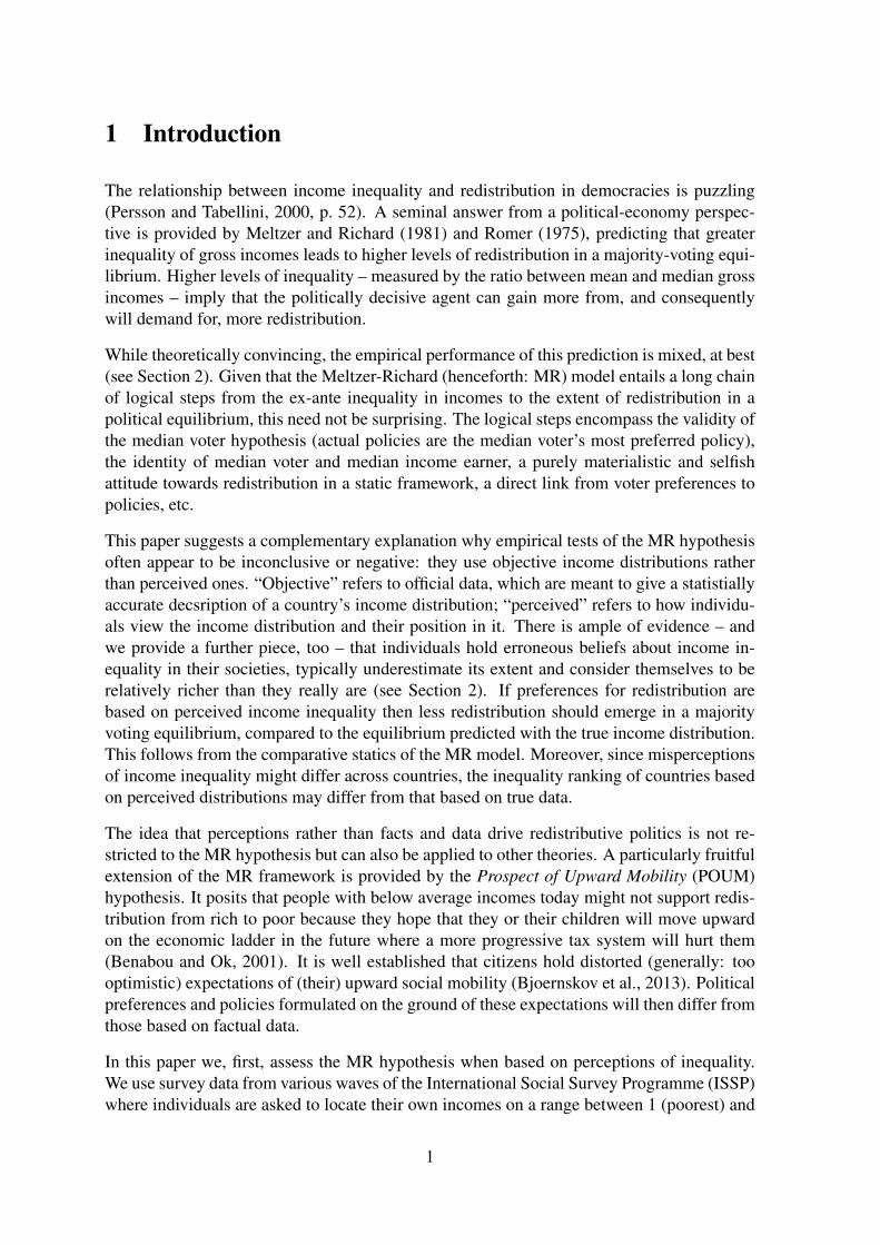
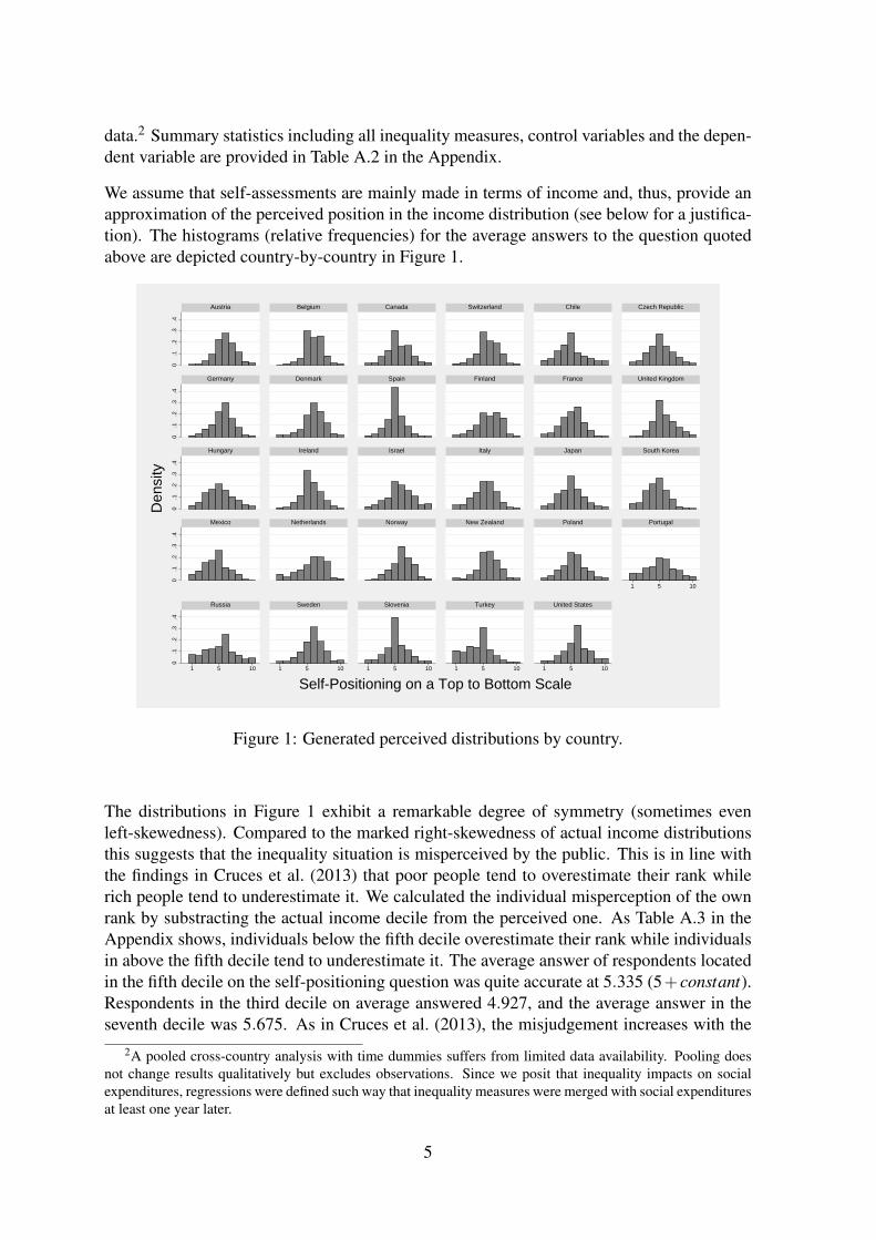
We assume that self-assessments are mainly made in terms of income and, thus, provide anapproximation of the perceived position in the income distribution (see below for a justifica-tion). The histograms (relative frequencies) for the average answers to the question quotedabove are depicted country-by-country in Figure 1.

0.1

.2.3

.40

.1.2

.3.4

0.1

.2.3

.40

.1.2

.3.4

0.1

.2.3

.4

1 5 10

1 5 10 1 5 10 1 5 10 1 5 10 1 5 10

Austria Belgium Canada Switzerland Chile Czech Republic

Germany Denmark Spain Finland France United Kingdom

Hungary Ireland Israel Italy Japan South Korea

Mexico Netherlands Norway New Zealand Poland Portugal

Russia Sweden Slovenia Turkey United States

Den

sity

Self-Positioning on a Top to Bottom Scale

Figure 1: Generated perceived distributions by country.

The distributions in Figure 1 exhibit a remarkable degree of symmetry (sometimes evenleft-skewedness). Compared to the marked right-skewedness of actual income distributionsthis suggests that the inequality situation is misperceived by the public. This is in line withthe findings in Cruces et al. (2013) that poor people tend to overestimate their rank whilerich people tend to underestimate it. We calculated the individual misperception of the ownrank by substracting the actual income decile from the perceived one. As Table A.3 in theAppendix shows, individuals below the fifth decile overestimate their rank while individualsin above the fifth decile tend to underestimate it. The average answer of respondents locatedin the fifth decile on the self-positioning question was quite accurate at 5.335 (5+constant).Respondents in the third decile on average answered 4.927, and the average answer in theseventh decile was 5.675. As in Cruces et al. (2013), the misjudgement increases with the

2A pooled cross-country analysis with time dummies suffers from limited data availability. Pooling doesnot change results qualitatively but excludes observations. Since we posit that inequality impacts on socialexpenditures, regressions were defined such way that inequality measures were merged with social expendituresat least one year later.

5

distance to the centre the distribution. Moreover, the results in Table A.3 suggest that whenanswering the ISSP question quoted above, respondents indeed associated the somewhatloose terms “groups in society”, “towards the top” or “towards the bottom” in accordancewith their view on income stratification.

The hypothetical income distributions in Figure 1 are based on the aggregation of individualand categorical data. They are, thus, not perceptions of the income distribution that any spe-cific individual in society holds but rather a summary view on how society categorizes itselfwith respect to inequality. According to the MR framework, the tax rate mostly preferred bythe median will win the voting. The higher the median perception of his position in society,the lower the prefered tax rate compared to the one which would have been chosen underperfect information.

To approximate the bias in perception, we compare the perceived mean to median ratio andthe actual one. We, first, define as the “perceived” mean-to-median ratio the ratio betweenthe average and the median value of self-categorizations. To capture the relative degree ofmisperception we form the ratio of the perceived mean-to-median ratio and the actual ratioone. We call this measure the “weighted perception” of income inequality:

weighted perception :=mean-to-median (perceived)

mean-to-median (actual).

Table 1 reports the actual mean-to-median ratios (calculated from OECD statistics), the per-ceived ratios, and the measure of weighted perceived inequality.

There are three remarkable observations:

• The actual mean-to-median ratios are uniformly greater than the perceived ones, in-dicating that inequality is underestimated everywhere. Correspondingly, the measureof weighted perceived inequality only takes values below 1. Its range from 0.986 to0.594 evidences that inequality is underestimated to a quite considerable degree.

• The degree of underestimation of inequality tends to be more pronounced in coun-tries with higher actual inequality: the coefficient of correlation between actual andperceived mean-to-median ratios is −0.36.

• In spite of this correlation, the country rankings with respect to actual and perceivedmean-to-median income ratios differ widely: the rank correlation coefficient is verylow at −0.06.

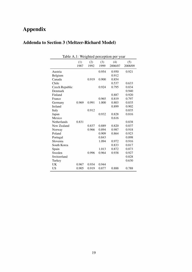
The numbers in Table 1 are based on cross-sectional data. Table A.1 in the Appendix reportsthe weighted perceived inequality measure per wave, confirming the widespread underesti-mation of inequality for every period.

6

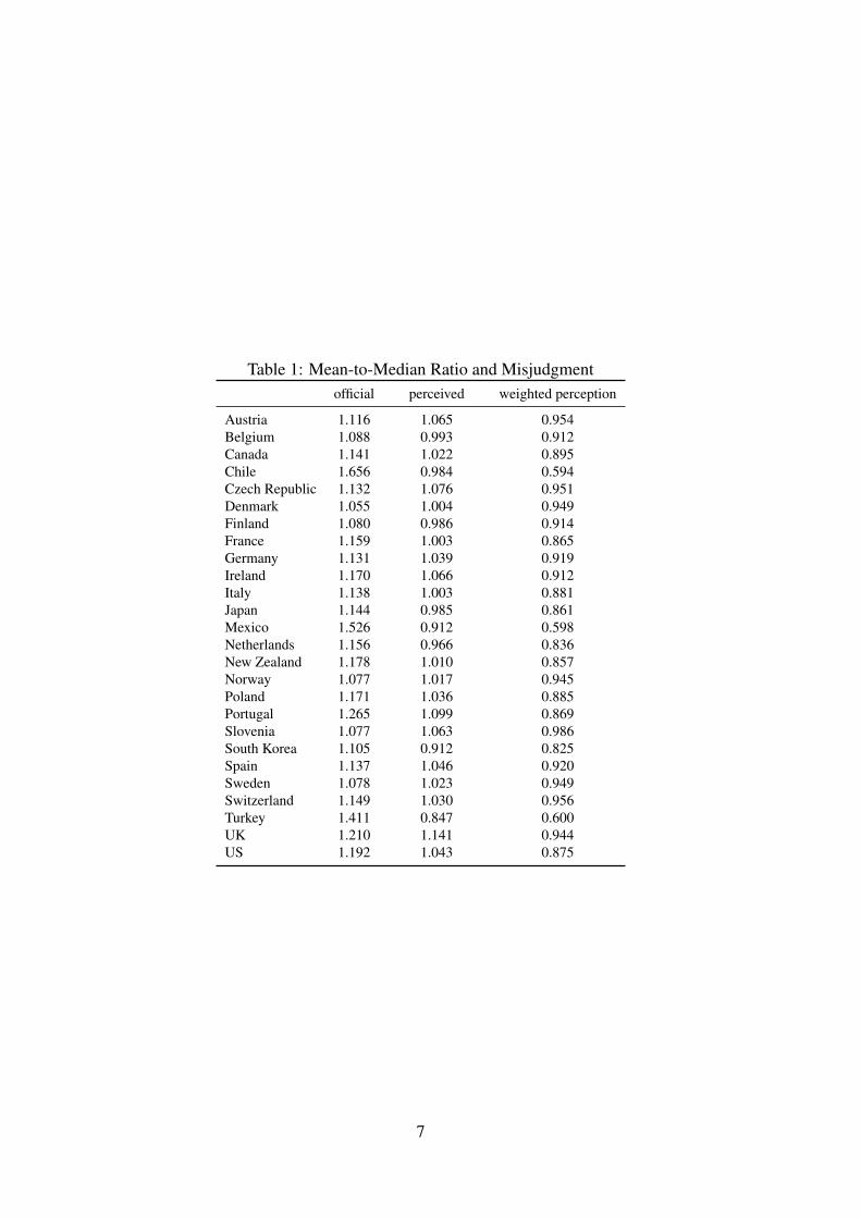
Table 1: Mean-to-Median Ratio and Misjudgmentofficial perceived weighted perception

Austria 1.116 1.065 0.954Belgium 1.088 0.993 0.912Canada 1.141 1.022 0.895Chile 1.656 0.984 0.594Czech Republic 1.132 1.076 0.951Denmark 1.055 1.004 0.949Finland 1.080 0.986 0.914France 1.159 1.003 0.865Germany 1.131 1.039 0.919Ireland 1.170 1.066 0.912Italy 1.138 1.003 0.881Japan 1.144 0.985 0.861Mexico 1.526 0.912 0.598Netherlands 1.156 0.966 0.836New Zealand 1.178 1.010 0.857Norway 1.077 1.017 0.945Poland 1.171 1.036 0.885Portugal 1.265 1.099 0.869Slovenia 1.077 1.063 0.986South Korea 1.105 0.912 0.825Spain 1.137 1.046 0.920Sweden 1.078 1.023 0.949Switzerland 1.149 1.030 0.956Turkey 1.411 0.847 0.600UK 1.210 1.141 0.944US 1.192 1.043 0.875

7

3.2 Empirical results

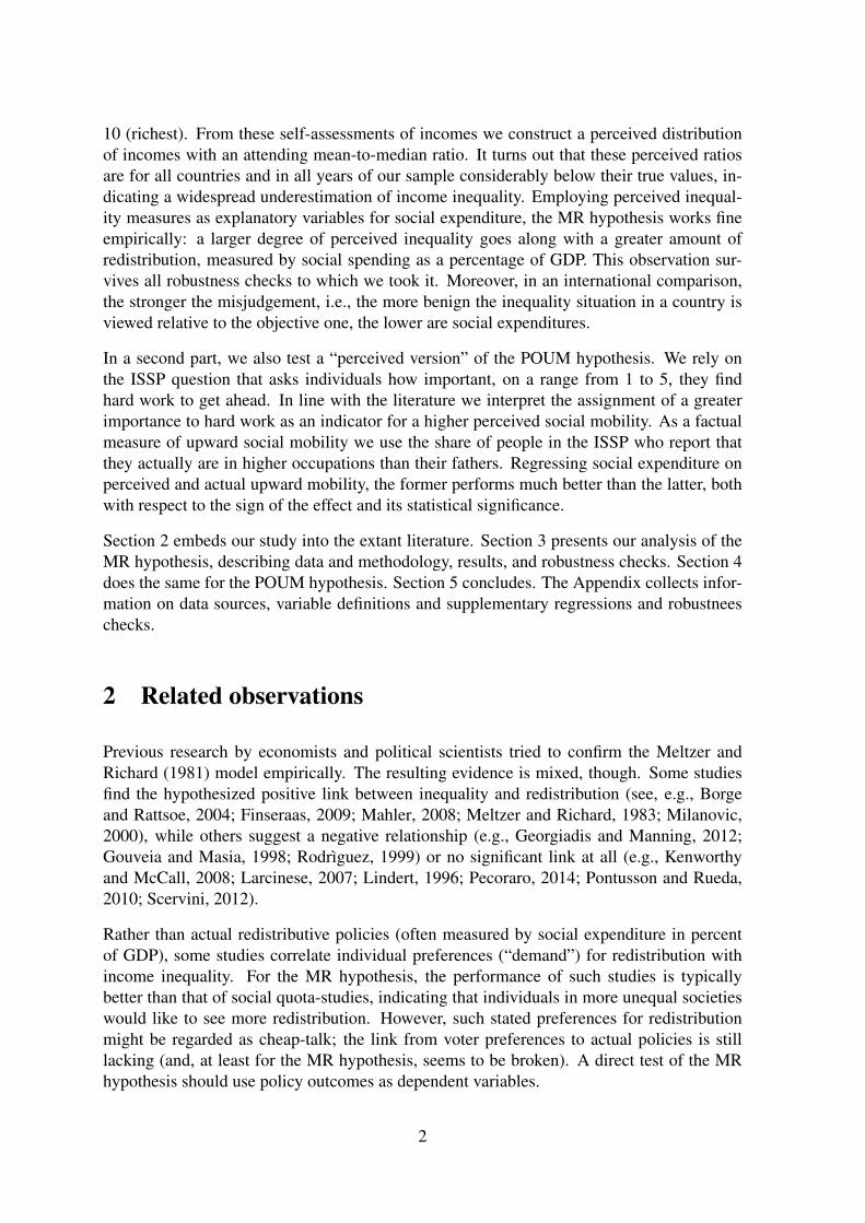
Figure 2 provides first insights into the relationship between social spending (taken from theOECD iLibrary) and the different inequality measures. Plotting social expenditures (in per-cent of GDP) against actual and perceived inequality in different countries shows a negativecorrelation between social expenditures and actual inequality (left panel), while social ex-penditure and the perceived inequality (middle and right panel) exhibit a positive association.

ATBE

CACH

CL

CZ

DE

DK

ES

FI

FR

GB

IE

IT

JP

KR MX

NLNO

NZPL PT

SE

SI

TR

US

510

1520

2530

Soc

ial E

xpen

ditu

res

(% o

f GD

P)

1 1.2 1.4 1.6 1.8Inequality (OECD)

ATBE

CACH

CL

CZ

DE

DK

ES

FI

FR

GB

IE

IT

JP

KRMX

NL NO

NZPL PT

SE

SI

TR

US

510

1520

2530

.8 .9 1 1.1 1.2Perceived Inequality

ATBE

CACH

CL

CZ

DE

DK

ES

FI

FR

GB

IE

IT

JP

KRMX

NL NO

NZPLPT

SE

SI

TR

US

510

1520

2530

.6 .7 .8 .9 1Weighted Perception

Figure 2: Misjudgment and social expenditures

Table 2 provides statistical support for these correlations.

Panel A of Table 2 reports the regressions, for various specifications, of social expenditures(in percent of GDP) on actual income inequality, i.e., on the ratio of mean to median incomebased on official OECD statistics. Specification (1) is the simple regression between actualinequality and social spending, while regressions (2) to (5) add further potential determinantsof social spending: current GDP (to capture the positive income elasticity of social spend-ing), the average of total exports and imports as a percentage of GDP (as a standard indicatorfor international trade openness), the dependency ratio (both to capture the necessity for so-cial spending), and average social expenditure in the 1980s (to capture the path-dependenceof social policies). Column (3) is the same as column (1) with data from the 1980s omit-ted, which are again included in columns (4) and (5) as independent variables. In conflictwith the predictions of the MR hypothesis – but quite in line with what previous studies also

8

Tabl

e2:

Mel

tzer

-Ric

hard

Mod

el

(1)

(2)

(3)

(4)

(5)

Pane

lAC

oef.

Std.

Err

.C

oef.

Std.

Err

.C

oef.

Std.

Err

.C

oef.

Std.

Err

.C

oef.

Std.

Err

.

ineq

ualit

y(O

EC

D)

-29.

95**

*(7

.738

)-3

2.04

**(1

4.47

)-2

9.46

***

(7.1

50)

-11.

98**

(5.6

17)

-22.

40**

(8.0

66)

soce

x80s

0.65

0***

(0.1

46)

0.64

6***

(0.1

59)

logG

DP

0.91

3(4

.409

)-3

.988

**(1

.418

)op

enne

ss0.

0353

(0.0

240)

-0.0

0950

(0.0

179)

depe

nden

cyra

tio1.

574*

*(0

.729

)0.

518

(0.4

38)

cons

tant

54.9

1***

(9.3

44)

-6.5

28(5

5.58

)54

.90*

**(8

.781

)23

.69*

*(9

.214

)60

.68*

**(1

8.52

)

R2

0.40

80.

607

0.39

40.

834

0.86

4N

2626

2626

26

(1)

(2)

(3)

(4)

(5)

Pane

lBC

oef.

Std.

Err

.C

oef.

Std.

Err

.C

oef.

Std.

Err

.C

oef.

Std.

Err

.C

oef.

Std.

Err

.

perc

eive

din

equa

lity

54.0

2**

(20.

17)

31.9

8*(1

7.30

)49

.95*

*(1

9.71

)21

.51*

(12.

46)

21.4

0(1

3.70

)so

cex8

0s0.

703*

**(0

.115

)0.

716*

**(0

.172

)lo

gGD

P7.

529*

*(3

.468

)-0

.082

4(1

.943

)op

enne

ss0.

0426

(0.0

346)

-0.0

0610

(0.0

277)

depe

nden

cyra

tio0.

911

(0.6

35)

-0.0

510

(0.3

18)

cons

tant

-35.

00(2

0.51

)-1

23.2

***

(36.

25)

-30.

18(1

9.98

)-1

2.96

(11.

09)

-10.

06(2

7.63

)

R2

0.24

40.

507

0.21

20.

819

0.82

0N

2626

2626

26

(1)

(2)

(3)

(4)

(5)

Pane

lCC

oef.

Std.

Err

.C

oef.

Std.

Err

.C

oef.

Std.

Err

.C

oef.

Std.

Err

.C

oef.

Std.

Err

.

wei

ghte

dpe

rcep

tion

44.7

7***

(6.7

24)

52.7

3***

(14.

41)

43.8

4***

(6.7

46)

20.4

3***

(6.0

40)

36.7

3***

(8.3

40)

soce

x80s

0.61

1***

(0.1

13)

0.62

1***

(0.1

00)

logG

DP

-1.6

98(3

.851

)-5

.259

**(2

.119

)op

enne

ss0.

0316

(0.0

263)

-0.0

103

(0.0

154)

depe

nden

cyra

tio1.

562*

**(0

.464

)0.

530

(0.3

13)

cons

tant

-19.

20**

*(5

.714

)-6

2.53

*(3

1.51

)-1

7.65

***

(5.5

86)

-7.4

09*

(3.6

35)

15.7

2(1

6.78

)

R2

0.52

00.

690

0.49

10.

861

0.90

8N

2626

2626

26

Rob

usts

tand

ard

erro

rsin

pare

nthe

ses:∗∗

∗p<

0.01

,∗∗

p<

0.05

,∗p<

0.1

Dep

ende

ntva

riab

le:

Soci

alex

pend

iture

sin

perc

ento

fGD

P

9

found –, the correlation between actual inequality and social spending is always significantlynegative, suggesting that lower inequality fosters redistribution.

Panel B of Table 2 reports the results from regressing, in the same sequence of specificationsas before, social expenditures (as a percentage of GDP) on perceived income inequality,as measured by the ratio of mean to median income in the distributions imputed from theanswers in the ISSP. The correlation between inequality and social expenditure now turnsout to be positive, in harmony with the MR hypothesis. In all but the last specification,the coefficient is statistically significant – and even the insignificant coefficient in the lastcolumn is more in line with the theory than the corresponding negative one in Panel A. Inessence, using perceived rather than actual inequality leads to a better performance of theMR hypothesis.

Since there exists a (negative) correlation between actual and perceived inequality (see Sec-tion 3.1) and a (negative) correlation between actual inequality and social spending, as shownin Panel A of Table 2, we have to include actual inequality to avoid provoking an omittedvariable bias. Therefore, Panel C in Table 2 reports the regressions of social expenditureon the weighted perception of inequality. The coefficients of the measure of weighted per-ceptions are highly statistically significant in all specifications and substantiate the positiverelationship.

Across all panels in Table 2, the coefficients of the control variables show the expected signs,when statistically significant. Only specification (5) does lead to an unexpected negative co-efficient of per-capita GDP. Excluding lagged social expenditures eliminates this unexpectedsign, which can be explained by the relatively high correlation between per-capita GDP andlagged social spending. This correlation impedes an efficient estimation of the correlationbetween both explanatory variables and the dependent variable.

In view of well-known endogeneity issues regressions of social spending on other variablesshould be interpreted with caution. We cannot fully resolve these issues, but try to capturethem by including lagged social spending as an independent variable. This decreases the ab-solute size of all coefficients for the inequality measures (see columns (4) and (5) in Table 2).It does not affect, however, the apparent difference in signs across panels. Out of caution, werefrain from economically interpreting the numerical magnitudes of coefficients. Still ourresults show that it is important to differentiate between actual and perceived inequality.

3.3 Robustness checks

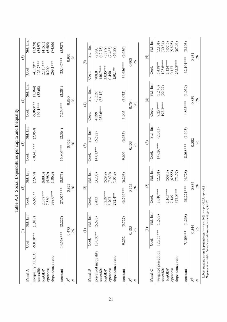
We subject our analysis to a variety of robustness checks, none of which qualitatively affectsour general conclusion. First, measuring the degree of redistribution by social expendituresper capita (rather than by its percentage in GDP) again produces a positive link betweenperceived inequality and redistribution (see Table A.4 in the Appendix).

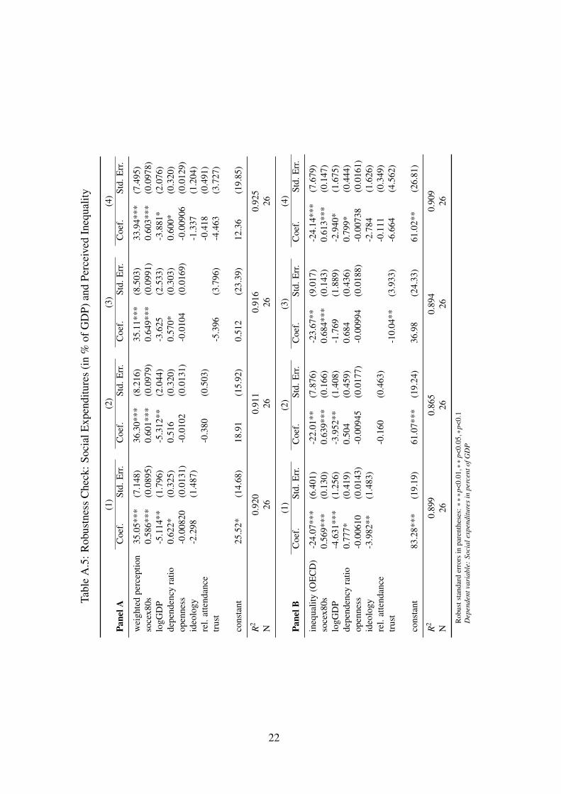
We also included variables that previous studies found to be imporant drivers for (a prefer-ence for) more redistribution. These include religious attendance, trust, and political ideol-ogy (left/right). We constructed quantitative measures for these variables, using data from

10

the World Values Surveys.3 The results reported in Panels A and B of Table A.5 in theAppendix show that, while statistically insignificant jointly, a more leftist attitude, a lowerdegree of trust and more frequent religious attendance ceteris paribus go along with moreredistribution (the latter only insignificantly). The associations between social spending andthe inequality measures remain unaffected, though.

Figure 2 suggests that Mexico, Turkey, South Korea and Chile might be outliers in our dataset. To rule out that statistical significance is driven by these countries, we also ran regres-sions that excluded them. This does not affect results in a significant way.4

4 The POUM hypothesis and perceived social mobility

4.1 Perceived vs. experienced social mobility

The POUM hypothesis posits that redistribution by the government is lower in democraciesthe higher is the degree of upward moility. As with the MR model in the previous sec-tion, we again argue that distinguishing between perceived and actual mobility is of crucialimportance when empirically testing this hypothesis.

The ISSP provides data that can be used to measure experienced (= actual) as well as per-ceived social upward mobility. A widely used measure of experienced mobility is based onthe following survey question:

“Please think about your present job (or your last one if you don’t have onenow). If you compare this job to the job your father had when you were14,15,16, would you say that the level of status of your job is (or was) . . . 1.Much lower than your father’s, 2. Lower, 3. About equal, 4. Higher or 5. Muchhigher than your father’s?”

The share of respondents who choose answers 4 or 5 (i.e., the fraction of people who thinkthey moved ahead of their fathers in their occupations) can serve as a measure of experiencedmobility in a society.5

A common measure of expected or perceived upward mobility is based on the hard-workquestion:

“Please tick one box to show how important you think hard work is for gettingahead in life (1 – not important at all; 5 – essential).”

3Data can also be obtained from the ISSP. We use the World Values Surveys to keep our sample constant(the ISSP lacks data for Belgium, Mexico, South Korea, Finland, and Turkey).

4Results are available on request. Essentially, regressions using the simple perceived inequality measurelose statistical significance, while maintaining their previous signs.

5When calculating the measure, we exclude all people who have never had a job or who do not know whattheir father did, never knew their father or whose father never had a job.

11

Higher numbers indicate a stronger perception that social structures are permeable. allowingfor upward mobility. For sake of comparability, we normalized this measure to the unitinterval, measuring the average importance of hard work for getting ahead.

Table 3: Upward mobility(1) (2)

experienced perceived

Austria 0.436 0.721Canada 0.501 0.740Chile 0.358 0.669Czech Republic 0.362 0.638Denmark 0.468 0.681Finland 0.482 0.744France 0.552 0.629Germany 0.420 0.696Hungary 0.411 0.646Italy 0.524 0.730Israel 0.482 0.677Japan 0.212 0.703New Zealand 0.438 0.784Norway 0.420 0.726Poland 0.504 0.724Portugal 0.600 0.703Slovenia 0.389 0.649South Korea 0.377 0.858Spain 0.523 0.675Sweden 0.391 0.718Switzerland 0.466 0.761Turkey 0.353 0.798UK 0.496 0.727US 0.500 0.816

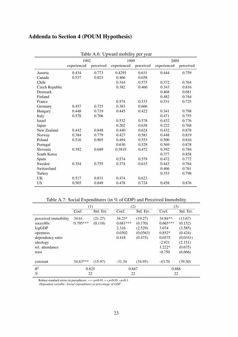
Table 3 reports the average values of experienced and expected mobility in our sample. Thesample covers the years in 1992, 1999 and 2009 for 24 OECD countries in the ISSP.6 Figuresper year are shown in Table A.6 in the Appendix. As can be seen from column (1), thelikelihood of being in a higher occupation than one’s father ranges from 0.212 in Japan to0.552 in France. Column (2) shows the values of perceived mobility which range between0.638 and 0.858. Thus, people in all countries tend to believe in the importance of hardwork to get ahead and therefore view their society as allowing for social mobility (albeit todifferent degrees).

4.2 Empirical results

Figure 3 visualizes a (positive) association between social expenditures (in percent of GDP)and experienced upward mobility as well as a (negative) correlation between social spending

6These are: Austria, Canada, Chile, Czech Republic, Denmark, Finland, France, Germany, Hungary, Italy,Israel, Japan, New Zealand, Norway, Poland, Portugal, Sweden, Slovenia, South Korea, Spain, Switzerland,Turkey, UK, and the US.

12

and perceived upward mobility. The contrast in directions is similar to what we encounteredfor the MR hypothesis.7

AT

CACH

CL

CZ

DE

DK

ES

FI

FR

GB

HU

IL

IT

JP

KR

NO

NZPL PT

SE

SI

TR

US

510

1520

2530

Soc

ial E

xpen

ditu

res

(% o

f GD

P)

.2 .3 .4 .5 .6Upward Mobility

AT

CACH

CL

CZ

DE

DK

ES

FI

FR

GB

HU

IL

IT

JP

KR

NO

NZPLPT

SE

SI

TR

US

510

1520

2530

.6 .65 .7 .75 .8 .85Perceived Upward Mobility

Figure 3: Redistribution and upward mobility

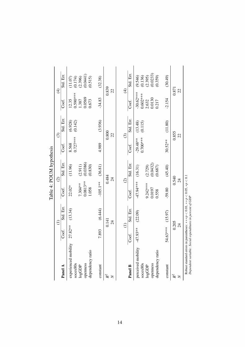
The regressions reported in Table 4 confirm the prima facie evidence of Figure 3:

The regressions of redistribution on experienced mobility in Panel A indicate – if anything– a weakly positive correlation between redistribution and social mobility, contradicting thePOUM hypothesis. Yet, except for the simple regression of column (1), the results are sta-tistically insignificant. By contrast, using perceptions as an explanatory variable vindicatesthe POUM hypothesis (see Panel B): the greater is perceived social mobility in a country, thesmaller is the extent of redistribution; all coefficients are statistically significant. Moreover,these observations are invariant across different specifications, which follow the same patternas in the previous section (see columns (1) to (4)).

4.3 Robustness checks

Again, we subjected our analysis to various robustness checks. First, we re-defined themeasure of actual (= experienced) mobility by calculating the probability of being in a muchbetter occupation than one’s father. This more restrictive definition renders all results based

7While cross-sectional data are used in Figure 3, we again checked that these correlations also hold forevery single time period.

13

Tabl

e4:

POU

Mhy

poth

esis

(1)

(2)

(3)

(4)

Pane

lAC

oef.

Std.

Err

.C

oef.

Std.

Err

.C

oef.

Std.

Err

.C

oef.

Std.

Err

.

expe

rien

ced

mob

ility

27.8

2**

(13.

34)

22.0

2*(1

1.96

)8.

568

(6.9

28)

12.3

5(1

1.07

)so

cex8

0s0.

727*

**(0

.142

)0.

590*

**(0

.174

)lo

gGD

P7.

304*

*(2

.911

)1.

387

(2.3

96)

open

ness

0.08

13**

(0.0

386)

0.05

69(0

.044

1)de

pend

ency

ratio

1.05

8(0

.830

)0.

673

(0.5

15)

cons

tant

7.89

3(6

.444

)-1

05.1

**(3

6.81

)4.

989

(3.9

36)

-34.

83(3

2.38

)

R2

0.14

10.

484

0.80

00.

839

N24

2422

22

(1)

(2)

(3)

(4)

Pane

lBC

oef.

Std.

Err

.C

oef.

Std.

Err

.C

oef.

Std.

Err

.C

oef.

Std.

Err

.

perc

eive

dm

obili

ty-4

7.93

**(2

2.09

)-4

7.94

***

(16.

31)

-29.

48**

(13.

48)

-30.

62**

*(9

.546

)so

cex8

0s0.

700*

**(0

.115

)0.

602*

**(0

.136

)lo

gGD

P9.

242*

**(2

.729

)2.

632

(2.3

95)

open

ness

0.01

97(0

.043

2)0.

0130

(0.0

233)

depe

nden

cyra

tio0.

558

(0.6

87)

0.21

7(0

.359

)

cons

tant

54.6

3***

(15.

97)

-59.

80(4

5.40

)30

.52*

*(1

1.80

)-2

.154

(30.

49)

R2

0.20

50.

540

0.85

50.

871

N24

2422

22

Rob

usts

tand

ard

erro

rsin

pare

nthe

ses:∗∗

∗p<

0.01

,∗∗

p<

0.05

,∗p<

0.1

Dep

ende

ntva

riab

le:

Soci

alex

pend

iture

sin

perc

ento

fGD

P

14

on experienced mobility statistically significant (but with coefficients still positive) and, thus,does not alter our general conclusion.

The “hard-work question”, though widely used in the literature, need not perfectly reflectexpected upward mobility: even if (one believes that) social mobility is low one could beconvinced of the importance of hard work for getting ahead. Therefore, we experimentedwith a measure of perceived immobility: it takes a value of one for a respondent who statesthat hard work is not important at all to get ahead (and value zero otherwise). For such arespondent we can assume that he does not believe in upward mobility. In line with thePOUM hypothesis we would expect that social spending increases with higher perceivedsocial immobility, measured by the population average of the immobility values. As can beseen in Table A.7 in the Appendix, this in fact holds empirically.

Table A.8 in the Appendix demonstrates that controlling for political and religious attitudescorroborates our findings: Panel A suggests that redistribution is lower the higher is ac-tual social mobility (thus, questioning the factual version of the POUM hypothesis), whilePanel B evidences a negative correlation between perceived mobility and social spending.

5 Concluding remarks

In democratic political systems the perceptions of the electorate on policy issues matter, po-tentially even more than objective data. If citizen-voters see an issue, politics has to respond– even if there is no issue; conversely, if a (real) problem is not salient with voters, it willprobably not be pursued forcefully.

This idea can be applied to “populist” politics of progressive tax-transfer problems. Ourstudy suggests that perceived inequality and expected upwards mobility are good predictorsof social policy, at least better ones than objective, offical or actual measures.

As a first attempt to trace social expenditures back to perceptions of inequality, our resultsare preliminary. But they open directions for future research. First, to check the stability ofour oberservations it will be interesting to repeat some of the more elaborate empirical stud-ies in the literature that test the MR or the POUM hypothesis with measures for perceivedinequality or social mobility, rather than with objective measures. Second, changing thedependent variable from actual social spending to preferences for redistribution will showwhether perceptions also matter for voters’ political demands and wishes. Third, while ourstudy takes perceptions as exogenous, one could study how these perceptions are shaped.This could then give rise to a more complete understanding of political choices in democ-racies. Finally, the discrepancies between perceptions and actual data might also matter forpolicy areas other than social spending.

15

Acknowledgments

The authors are grateful to Carsten Schroeder and Frank Neher for fruitful discussions andadvice. Seminar and conference participants in Hannover and Berlin provided helpful com-ments. The usual disclaimer applies.

ReferencesAlesina, A., La Ferrara, E., 2005. Preferences for redistribution in the land of opportunities.

Journal of Public Economics 89, 897–931.

Bartels, L. M., 2005. Homer gets a tax cut: Inequality and public policy in the Americanmind. Perspectives on Politics 3, 15–31.

Bartels, L. M., 2008. Unequal Democracy: The Political Economy of the New Gilded Age.Princeton University Press, Princeton, NJ.

Benabou, R., Ok, E. A., 2001. Social mobility and the demand for redistribution: The POUMhypothesis. Quarterly Journal of Economics 116, 447–487.

Bjoernskov, C., Dreher, A., Fischer, J. A., Schnellenbach, J., Gehring, K., 2013. Inequal-ity and happiness: When perceived social mobility and economic reality do not match.Journal of Economic Behavior and Organization 91, 75–92.

Borge, L.-E., Rattsoe, J., 2004. Income distribution and tax structure: Empirical test of theMeltzer-Richard hypothesis. European Economic Review 48, 805–826.

Bredemeier, C., 2014. Imperfect information and the Meltzer-Richard hypothesis. PublicChoice 159, 561–576.

Brooks, C., Manza, J., 2006. Social policy responsiveness in developed democracies. Amer-ican Sociological Review 71, 474–494.

Corneo, G., Grüner, H.-P., 2002. Individual preferences for political redistribution. Journalof Public Economics 83, 83–107.

Cruces, G., Perez-Truglia, R., Tetaz, M., 2013. Biased perception of income distributionand preferences for redistribution: Evidence from a survey experiment. Journal of PublicEconomics 98, 100–112.

Evans, M., Kelley, J., 2004. Subjective social location: Data from 21 nations. InternationalJournal of Public Opinion Research 16, 3–38.

Finseraas, H., 2009. Income inequality and demand for redistribution: A multilevel analysisof European public opinion. Scandinavian Political Studies 32 (1), 94–119.

Fujii, E. T., Hawley, C. B., 1988. On the accuracy of tax perceptions. Review of Economicsand Statistics 70 (2), 344–47.

16

Gärling, T., Gamble, A., 2008. Perceived inflation and expected future prices in differentcurrencies. Journal of Economic Psychology 29 (4), 401–416.

Georgiadis, A., Manning, A., 2012. Spend it like Beckham? Inequality and redistribution inthe UK, 1983-2004. Public Choice 151, 537–563.

Gouveia, M., Masia, N. A., 1998. Does the median voter model explain the size of govern-ment? evidence from the States. Public Choice 97, 159–177.

Guenther, C. L., Alicke, M. D., 2010. Deconstructing the Better-than-Average effect. Journalof Personality and Social Psychology 99, 755–770.

Jacob, B. A., Lefgren, L., 2008. Can principals identify effective teachers? evidence onsubjective performance evaluation in education. Journal of Labor Economics 26, 101–136.

Kenworthy, L., McCall, L., 2008. Inequality, public opinion and redistribution. Socio-Economic Review 6, 35–68.

Larcinese, V., 2007. Voting over redistribution and the size of the welfare state. PoliticalStudies 55, 565–585.

Lindert, P., 1996. What limits social spending? Explorations in Economic History 33, 1–34.

Lübker, M., 2006. Inequality and the demand for redistribution: Are assumptions of the newgrowth theory valid? Socio-Economic Review 5, 117–148.

Mahler, V. A., 2008. Electoral turnout and income redistribution by the state: A cross-national analysis of developed democracies. European Journal of Political Research 47,161–183.

Meltzer, A. H., Richard, S. F., 1981. A rational theory of the size of government. The Journalof Political Economy 89 (5), 914–927.

Meltzer, A. H., Richard, S. F., 1983. Tests of a rational theory of the size of government.Public Choice 41 (3), 403–418.

Milanovic, B., 2000. The median-voter hypothesis, income inequality, and income redistri-bution: An empirical test with the required data. European Journal of Political Economy16 (3), 367–410.

Niehues, J., 2014. Subjective perceptions of inequality and redistributive preferences: An in-ternational comparison. Discussion paper, Cologne Institute for Economic Research (IW).

Norton, M. I., Ariely, D., 2011. Building a better America – one wealth quintile at a time.Perspectives on Psychological Science 6, 9–12.

Olken, B. A., 2009. Corruption perceptions vs. corruption reality. Journal of Public Eco-nomics 93 (7-8), 950–964.

Osberg, L., Smeeding, T., 2006. “Fair” inequality? Attitudes toward pay differentials: TheUnited States in comparative perspective. American Sociological Review 71, 450–473.

17

Pecoraro, B., 2014. Inequality in democracies: Testing the classic democratic theory of re-distribution. Economics Letters 123, 398–401.

Persson, T., Tabellini, G., 2000. Political Economics: Explaining Economic Policy. The MITPress, Cambridge, MA.

Pontusson, J., Rueda, D., 2010. The politics of inequality: Voter mobilization and left partiesin advances industrial states. Comparative Political Studies 43, 675–705.

Rodrìguez, F. C., 1999. Does distributional skewness lead to redistribution? Evidence fromthe United States. Economics and Politics 11 (2), 171–199.

Romer, T., 1975. Individual welfare, majority voting and the properties of a linear incometax. Journal of Public Economics 4 (2), 163–185.

Runciman, W. G., 1966. Relative Deprivation and Social Justice: A Study of Attitudes toSocial Inequality in Twentieth-Century England. Routledge Kegan Paul, London.

Scervini, F., 2012. Empirics of the median voter: Democracy, redistribution and the role ofthe middle class. Journal of Economic Inequality 10, 529–550.

18

Appendix

Addenda to Section 3 (Meltzer-Richard Model)

Table A.1: Weighted perception per year(1) (2) (3) (4) (5)

1987 1992 1999 2006/07 2008/09

Austria 0.954 0.950 0.921Belgium 0.912Canada 0.919 0.900 0.854Chile 0.537 0.633Czech Republic 0.924 0.795 0.834Denmark 0.940Finland 0.887 0.920France 0.965 0.819 0.797Germany 0.969 0.991 1.000 0.803 0.835Ireland 0.899 0.902Italy 0.912 0.835Japan 0.932 0.828 0.816Mexico 0.616Netherlands 0.831 0.838New Zealand 0.837 0.889 0.820 0.837Norway 0.966 0.894 0.987 0.918Poland 0.909 0.864 0.923Portugal 0.843 0.898Slovenia 1.094 0.972 0.916South Korea 0.833 0.817Spain 1.013 0.872 0.873Sweden 0.996 0.964 0.938 0.927Switzerland 0.828Turkey 0.630UK 0.967 0.934 0.944US 0.905 0.919 0.877 0.888 0.788

19

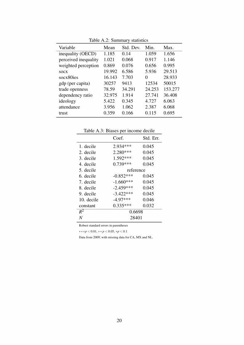
Table A.2: Summary statisticsVariable Mean Std. Dev. Min. Max.inequality (OECD) 1.185 0.14 1.059 1.656perceived inequality 1.021 0.068 0.917 1.146weighted perception 0.869 0.076 0.656 0.995socx 19.992 6.586 5.936 29.513socx80ies 16.143 7.703 0 28.933gdp (per capita) 30257 9413 12534 50015trade openness 78.59 34.291 24.253 153.277dependency ratio 32.975 1.914 27.741 36.408ideology 5.422 0.345 4.727 6.063attendance 3.956 1.062 2.387 6.068trust 0.359 0.166 0.115 0.695

Table A.3: Biases per income decileCoef. Std. Err.

1. decile 2.934*** 0.0452. decile 2.280*** 0.0453. decile 1.592*** 0.0454. decile 0.739*** 0.0455. decile reference6. decile -0.852*** 0.0457. decile -1.660*** 0.0458. decile -2.459*** 0.0459. decile -3.422*** 0.04510. decile -4.97*** 0.046constant 0.335*** 0.032R2 0.6698N 28401Robust standard errors in parentheses

∗∗∗p < 0.01, ∗∗ p < 0.05, ∗p < 0.1

Data from 2009; with missing data for CA, MX and NL.

20

Tabl

eA

.4:S

ocia

lExp

endi

ture

spe

rcap

itaan

dIn

equa

lity

(1)

(2)

(3)

(4)

(5)

Pane

lAC

oef.

Std.

Err

.C

oef.

Std.

Err

.C

oef.

Std.

Err

.C

oef.

Std.

Err

.C

oef.

Std.

Err

.

ineq

ualit

y(O

EC

D)

-9,0

10**

*(1

,817

)-5

,653

**(2

,679

)-1

0,41

3***

(2,0

59)

-5,0

60**

*(1

,364

)-4

,179

**(1

,920

)so

cxx8

0s19

9.1*

**(3

2.68

)12

3.7*

**(3

4.97

)lo

gGD

P2,

337*

**(6

80.3

)2,

113*

**(4

15.1

)op

enne

ss7.

560

(5.9

89)

0.20

9(5

.585

)de

pend

ency

ratio

398.

0***

(106

.3)

269.

1***

(74.

66)

cons

tant

14,5

68**

*(2

,227

)-2

7,07

5***

(8,8

71)

16,8

06**

*(2

,564

)7,

250*

**(2

,201

)-2

3,14

7***

(5,9

27)

R2

0.47

50.

827

0.45

20.

830

0.93

1N

2626

2626

26

(1)

(2)

(3)

(4)

(5)

Pane

lBC

oef.

Std.

Err

.C

oef.

Std.

Err

.C

oef.

Std.

Err

.C

oef.

Std.

Err

.C

oef.

Std.

Err

.

perc

eive

din

equa

lity

13,0

50**

(5,6

73)

2,43

3(3

,203

)14

,013

**(6

,582

)4,

599

(3,5

59)

708.

8(2

,980

soce

x80s

232.

6***

(35.

12)

140.

7***

(42.

75)

logG

DP

3,75

9***

(529

.9)

3,03

5***

(337

.8)

open

ness

8.70

7(7

.630

)0.

450

(7.4

83)

depe

nden

cyra

tio27

2.4*

*(1

05.9

)15

0.1*

*(6

4.38

)

cons

tant

-9,2

52(5

,727

)-4

6,74

6***

(6,2

93)

-9,6

06(6

,635

)-3

,905

(3,0

72)

-34,

636*

**(6

,636

)

R2

0.18

30.

765

0.15

30.

764

0.90

8N

2626

2626

26

(1)

(2)

(3)

(4)

(5)

Pane

lCC

oef.

Std.

Err

.C

oef.

Std.

Err

.C

oef.

Std.

Err

.C

oef.

Std.

Err

.C

oef.

Std.

Err

.

wei

ghte

dpe

rcep

tion

12,7

55**

*(1

,578

)8,

010*

**(2

,281

)14

,626

***

(2,0

33)

7,25

7***

(1,5

40)

5,43

8**

(2,1

01)

soce

x80s

192.

3***

(22.

27)

123.

6***

(30.

34)

logG

DP

2,16

5***

(558

.3)

2,12

4***

(457

.5)

open

ness

7.14

9(6

.555

)0.

127

(5.8

95)

depe

nden

cyra

tio37

7.8*

**(7

1.57

)24

5.8*

**(6

7.04

)

cons

tant

-7,1

09**

*(1

,268

)-3

8,22

1***

(4,7

28)

-8,0

88**

*(1

,603

)-4

,865

***

(1,0

59)

-32,

101*

**(5

,103

)

R2

0.54

40.

834

0.50

20.

839

0.93

1N

2626

2626

26

Rob

usts

tand

ard

erro

rsin

pare

nthe

ses:∗∗

∗p<

0.01

,∗∗

p<

0.05

,∗p<

0.1

Dep

ende

ntva

riab

le:

Soci

alex

pend

iture

sas

perc

enta

geof

GD

P

21

Tabl

eA

.5:R

obus

tnes

sC

heck

:Soc

ialE

xpen

ditu

res

(in

%of

GD

P)an

dPe

rcei

ved

Ineq

ualit

y

(1)

(2)

(3)

(4)

Pane

lAC

oef.

Std.

Err

.C

oef.

Std.

Err

.C

oef.

Std.

Err

.C

oef.

Std.

Err

.

wei

ghte

dpe

rcep

tion

35.0

5***

(7.1

48)

36.3

0***

(8.2

16)

35.1

1***

(8.5

03)

33.9

4***

(7.4

95)

soce

x80s

0.58

6***

(0.0

895)

0.60

1***

(0.0

979)

0.64

9***

(0.0

991)

0.60

3***

(0.0

978)

logG

DP

-5.1

14**

(1.7

96)

-5.3

12**

(2.0

44)

-3.6

25(2

.533

)-3

.881

*(2

.076

)de

pend

ency

ratio

0.62

2*(0

.325

)0.

516

(0.3

20)

0.57

0*(0

.303

)0.

600*

(0.3

20)

open

ness

-0.0

0820

(0.0

131)

-0.0

102

(0.0

131)

-0.0

104

(0.0

169)

-0.0

0906

(0.0

129)

ideo

logy

-2.2

98(1

.487

)-1

.337

(1.2

04)

rel.

atte

ndan

ce-0

.380

(0.5

03)

-0.4

18(0

.491

)tr

ust

-5.3

96(3

.796

)-4

.463

(3.7

27)

cons

tant

25.5

2*(1

4.68

)18

.91

(15.

92)

0.51

2(2

3.39

)12

.36

(19.

85)

R2

0.92

00.

911

0.91

60.

925

N26

2626

26

(1)

(2)

(3)

(4)

Pane

lBC

oef.

Std.

Err

.C

oef.

Std.

Err

.C

oef.

Std.

Err

.C

oef.

Std.

Err

.

ineq

ualit

y(O

EC

D)

-24.

07**

*(6

.401

)-2

2.01

**(7

.876

)-2

3.67

**(9

.017

)-2

4.14

***

(7.6

79)

soce

x80s

0.56

9***

(0.1

30)

0.63

9***

(0.1

66)

0.68

4***

(0.1

43)

0.61

3***

(0.1

47)

logG

DP

-4.6

31**

*(1

.256

)-3

.952

**(1

.408

)-1

.769

(1.8

89)

-2.9

40*

(1.6

75)

depe

nden

cyra

tio0.

777*

(0.4

19)

0.50

4(0

.459

)0.

684

(0.4

36)

0.79

9*(0

.444

)op

enne

ss-0

.006

10(0

.014

3)-0

.009

45(0

.017

7)-0

.009

94(0

.018

8)-0

.007

38(0

.016

1)id

eolo

gy-3

.982

**(1

.483

)-2

.784

(1.6

26)

rel.

atte

ndan

ce-0

.160

(0.4

63)

-0.1

11(0

.349

)tr

ust

-10.

04**

(3.9

33)

-6.6

64(4

.562

)

cons

tant

83.2

8***

(19.

19)

61.0

7***

(19.

24)

36.9

8(2

4.33

)61

.02*

*(2

6.81

)

R2

0.89

90.

865

0.89

40.

909

N26

2626

26

Rob

usts

tand

ard

erro

rsin

pare

nthe

ses:∗∗

∗p<0

.01,∗∗

p<0.

05,∗

p<0.

1D

epen

dent

vari

able

:So

cial

expe

nditu

res

inpe

rcen

tofG

DP

22

Addenda to Section 4 (POUM Hypothesis)

Table A.6: Upward mobility per year1992 1999 2009

experienced perceived experienced perceived experienced perceived

Austria 0.434 0.773 0.4293 0.631 0.444 0.759Canada 0.537 0.823 0.466 0.658Chile 0.344 0.575 0.372 0.764Czech Republic 0.382 0.460 0.343 0.816Denmark 0.468 0.681Finland 0.482 0.744France 0.574 0.533 0.531 0.725Germany 0.457 0.725 0.383 0.666Hungary 0.448 0.719 0.445 0.422 0.341 0.798Italy 0.578 0.706 0.471 0.755Israel 0.532 0.578 0.432 0.776Japan 0.202 0.638 0.222 0.768New Zealand 0.442 0.848 0.440 0.624 0.432 0.878Norway 0.384 0.779 0.427 0.581 0.448 0.819Poland 0.516 0.805 0.494 0.553 0.500 0.816Portugal 0.630 0.529 0.569 0.878Slovenia 0.392 0.689 0.3819 0.472 0.392 0.784South Korea 0.377 0.858Spain 0.574 0.579 0.472 0.772Sweden 0.354 0.755 0.374 0.615 0.443 0.784Switzerland 0.466 0.761Turkey 0.353 0.798UK 0.517 0.831 0.474 0.623US 0.565 0.849 0.478 0.724 0.458 0.876

Table A.7: Social Expenditures (in % of GDP) and Perceived Immobility(1) (2) (3)

Coef. Std. Err. Coef. Std. Err. Coef. Std. Err.

perceived immobility 34.61 (21.27) 34.23* (19.27) 34.84** (13.67)socex80s 0.795*** (0.118) 0.681*** (0.170) 0.665*** (0.152)logGDP 2.316 (2.529) 3.074 (3.585)openness 0.0302 (0.0363) 0.852* (0.424)dependency ratio 0.418 (0.475) 0.0575 (0.0341)ideology -2.921 (2.151)rel. attendance 1.222* (0.675)trust -0.750 (6.666)

constant 54.63*** (15.97) -31.34 (34.95) -43.70 (39.30)

R2 0.825 0.847 0.888N 22 22 22

Robust standard errors in parentheses: ∗∗∗p<0.01,∗∗ p<0.05,∗p<0.1Dependent variable: Social expenditures as percentage of GDP

23

Tabl

eA

.8:S

ocia

lExp

endi

ture

s(%

gdp)

and

Perc

eive

dM

obili

ty-R

obus

tnes

sC

heck

(1)

(2)

(3)

(4)

Pane

lAC

oef.

Std.

Err

.C

oef.

Std.

Err

.C

oef.

Std.

Err

.C

oef.

Std.

Err

.

perc

eive

dm

obili

ty-2

6.27

**(9

.812

)-3

3.10

***

(9.8

98)

-24.

86**

(10.

37)

-26.

86**

(11.

14)

soce

x80s

0.59

6***

(0.1

38)

0.60

7***

(0.1

14)

0.63

7***

(0.1

36)

0.62

0***

(0.1

34)

logG

DP

2.37

3(2

.488

)3.

418

(2.2

87)

4.04

7(3

.057

)3.

922

(3.5

16)

depe

nden

cyra

tio0.

298

(0.4

28)

0.51

6(0

.346

)0.

383

(0.3

91)

0.64

2(0

.363

)op

enne

ss0.

0188

(0.0

234)

0.03

39(0

.022

6)0.

0260

(0.0

261)

0.04

36(0

.025

2)id

eolo

gy-1

.425

(1.6

11)

-1.0

14(1

.889

)re

l.at

tend

ance

1.17

6**

(0.5

19)

1.10

5*(0

.619

)tr

ust

-5.9

06(4

.358

)-3

.069

(6.3

40)

cons

tant

2.10

8(3

1.70

)-2

4.30

(27.

39)

-25.

65(4

1.41

)-3

2.14

(42.

75)

R2

0.87

50.

889

0.88

00.

895

N22

2222

22

(1)

(2)

(3)

(4)

Pane

lBC

oef.

Std.

Err

.C

oef.

Std.

Err

.C

oef.

Std.

Err

.C

oef.

Std.

Err

.

expe

rien

ced

mob

ility

7.96

6(1

2.04

)10

.92

(11.

76)

6.41

7(1

1.50

)2.

360

(13.

11)

soce

x80s

0.59

2***

(0.1

59)

0.60

2***

(0.1

70)

0.65

9***

(0.1

59)

0.65

9***

(0.1

56)

logG

DP

1.25

5(2

.538

)1.

702

(2.5

12)

3.76

1(3

.206

)3.

451

(3.4

52)

depe

nden

cyra

tio0.

677

(0.5

25)

0.79

5(0

.541

)0.

748

(0.5

11)

0.90

6(0

.512

)op

enne

ss0.

0550

(0.0

406)

0.06

63(0

.048

6)0.

0615

(0.0

430)

0.07

23(0

.043

8)id

eolo

gy-2

.375

(1.7

94)

-1.9

65(2

.152

)re

l.at

tend

ance

0.52

9(0

.756

)0.

766

(0.7

60)

trus

t-8

.467

(5.0

65)

-6.1

22(5

.599

)

cons

tant

-18.

70(3

3.70

)-4

4.33

(35.

23)

-57.

39(4

0.34

)-5

1.54

(41.

50)

R2

0.85

10.

842

0.85

50.

865

N22

2222

22

Rob

usts

tand

ard

erro

rsin

pare

nthe

ses:∗∗

∗p<0

.01,∗∗

p<0.

05,∗

p<0.

1D

epen

dent

vari

able

:So

cial

expe

nditu

rein

perc

ento

fGD

P

24