Bi-Clustering

Jinze Liu

Outline

• The Curse of Dimensionality

• Co-Clustering Partition-based hard clustering

• Subspace-ClusteringPattern-based

2

3

Clustering

k

t citi

t

cxdist1

2),(

m

jtjijti cxcxdist

1

2)(),(WhereK-means clustering minimizes

The Curse of Dimensionality

The dimension of a problem refers to the number of input variables (actually, degrees of freedom).

The curse of dimensionality

•The exponential increase in data required to densely populate space as the dimension increases.

•The points are equally far apart in high dimensional space.

1–D

2–D 3–D

Motivation

5

110000000

111000000

011100000

100000010

000001100

000010010

000010010

000002110

000010110

000000011

000000101

000001001

Doc

Term

Document Clustering:

Define a similarity measure

Clustering the documents using e.g. k-means

Term Clustering:

Symmetric with Doc Clustering

Motivation

6

Genes

Patients

Hierarchical Clustering of Genes

Hierarchical Clustering of Patients

Contingency Tables• Let X and Y be discrete random variables

X and Y take values in {1, 2, …, m} and {1, 2, …, n}

p(X, Y) denotes the joint probability distribution—if not known, it is often estimated based on co-occurrence data

Application areas: text mining, market-basket analysis, analysis of browsing behavior, etc.

• Key Obstacles in Clustering Contingency Tables High Dimensionality, Sparsity, Noise Need for robust and scalable algorithms

Co-Clustering

• SimultaneouslyCluster rows of p(X, Y) into k disjoint groups Cluster columns of p(X, Y) into l disjoint groups

• Key goal is to exploit the “duality” between row and column clustering to overcome sparsity and noise

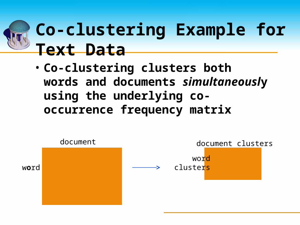
Co-clustering Example for Text Data

document

wordword

clusters

document clusters

• Co-clustering clusters both words and documents simultaneously using the underlying co-occurrence frequency matrix

Result of Co-Clustering

10

http://adios.tau.ac.il/SpectralCoClustering/

http://adios.tau.ac.il/SpectralCoClustering/

A presentation topic – Hierarchical Co-Clustering

Clustering by Patterns

11

12

Clustering by Pattern Similarity (p-Clustering)

• The micro-array “raw” data shows 3 genes and their values

in a multi-dimensional space Parallel Coordinates Plots

Difficult to find their patterns

• “non-traditional”

clustering

13

Clusters Are Clear After Projection

14

Motivation

• E-Commerce: collaborative filtering

Movie 1

Movie 2

Movie 3

Movie 4

Movie 5

Movie 6

Movie 7

Viewer 1 1 2 4 3 5

Viewer 2 4 6 7 1

Viewer 3 2 3 4 6 3

Viewer 4 3 4 5 7

Viewer 5 5 5 3 4

15

Motivation

012345678

rating

viewer 1

viewer 2

viewer 3

viewer 4

viewer 5

16

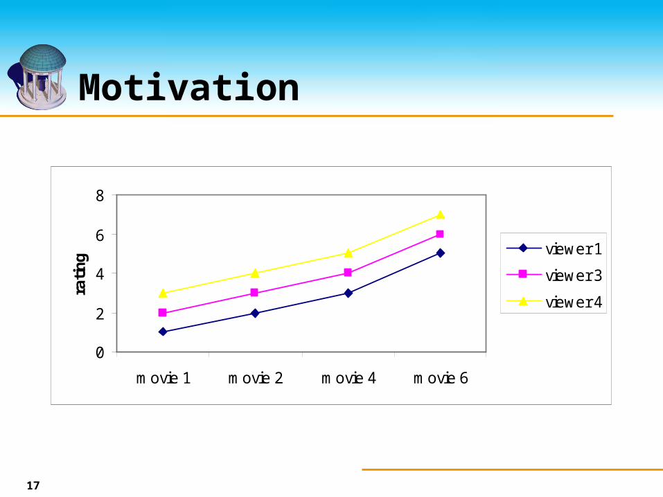
Motivation

Movie 1

Movie 2

Movie 3

Movie 4

Movie 5

Movie 6

Movie 7

Viewer 1 1 2 4 3 5

Viewer 2 4 6 7 1

Viewer 3 2 3 4 6 3

Viewer 4 3 4 5 7

Viewer 5 5 5 3 4

17

Motivation

0

2

4

6

8

movie 1 movie 2 movie 4 movie 6

rating

viewer 1

viewer 3

viewer 4

18

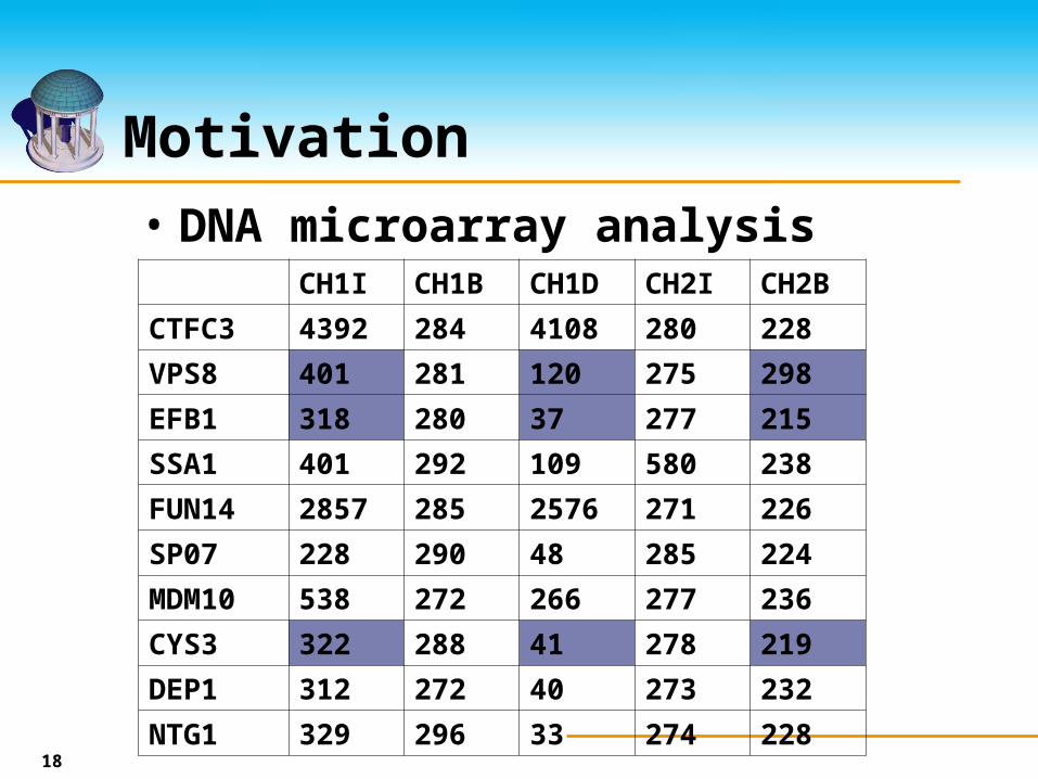
Motivation• DNA microarray analysis

CH1I CH1B CH1D CH2I CH2B

CTFC3 4392 284 4108 280 228

VPS8 401 281 120 275 298

EFB1 318 280 37 277 215

SSA1 401 292 109 580 238

FUN14 2857 285 2576 271 226

SP07 228 290 48 285 224

MDM10 538 272 266 277 236

CYS3 322 288 41 278 219

DEP1 312 272 40 273 232

NTG1 329 296 33 274 228

19

Motivation

0

50100

150

200250

300

350400

450

CH1I CH1D CH2B

condition

strength

20

Motivation

• Strong coherence exhibits by the selected objects on the selected attributes.They are not necessarily close to each other but

rather bear a constant shift.Object/attribute bias

• bi-cluster

21

Challenges

• The set of objects and the set of attributes are usually unknown.

• Different objects/attributes may possess different biases and such biasesmay be local to the set of selected

objects/attributesare usually unknown in advance

• May have many unspecified entries

22

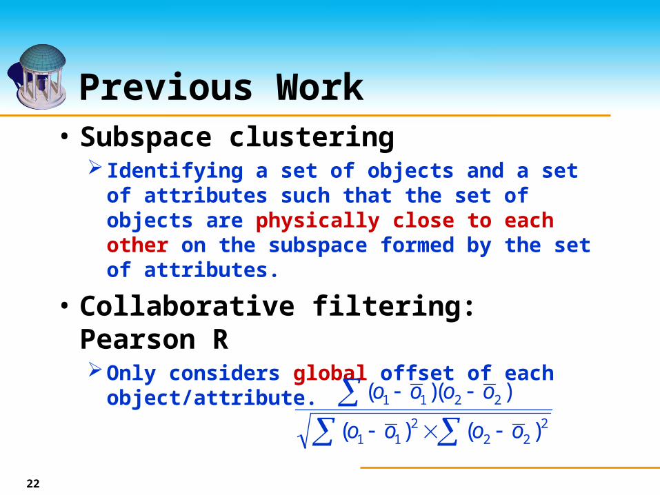
Previous Work• Subspace clustering

Identifying a set of objects and a set of attributes such that the set of objects are physically close to each other on the subspace formed by the set of attributes.

• Collaborative filtering: Pearson ROnly considers global offset of each object/attribute.

2

222

11

2211

)()(

))((

oooo

oooo

23

bi-cluster

• Consists of a (sub)set of objects and a (sub)set of attributesCorresponds to a submatrixOccupancy threshold

Each object/attribute has to be filled by a certain percentage.

Volume: number of specified entries in the submatrix

Base: average value of each object/attribute (in the bi-cluster)

24

bi-cluster

CH1I CH1B CH1D CH2I CH2B Obj base

CTFC3

VPS8 401 120 298 273

EFB1 318 37 215 190

SSA1

FUN14

SP07

MDM10

CYS3 322 41 219 194

DEP1

NTG1

Attr base 347 66 244 219

25

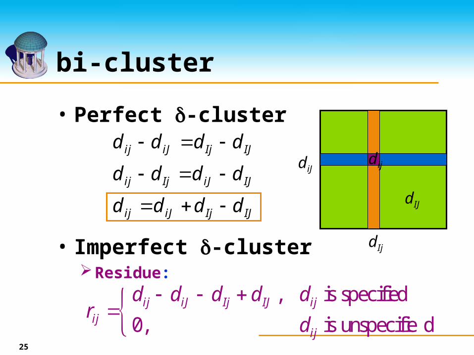
bi-cluster

• Perfect -cluster

• Imperfect -clusterResidue:

IJIjiJij

IJiJIjij

IJIjiJij

dddd

dddd

dddd

îíì

dunspecifie is ,0

specified is ,

ij

ijIJIjiJijij d

dddddr

dIJ

dIj

diJ dij

26

bi-cluster

• The smaller the average residue, the stronger the coherence.

• Objective: identify -clusters with residue smaller than a given threshold

27

Cheng-Church Algorithm

• Find one bi-cluster.

• Replace the data in the first bi-cluster with random data

• Find the second bi-cluster, and go on.

• The quality of the bi-cluster degrades (smaller volume, higher residue) due to the insertion of random data.

28

The FLOC algorithm

Generating initial clusters

Determine the best action for each row and each column

Perform the best action of each row and column sequentially

Improved?Y

N

29

The FLOC algorithm

• Action: the change of membership of a row(or column) with respect to a cluster

3 4

4

1 3

2 2

3

2

2

0 4

column

row 1

3

2

1

2 3 4

M+N actions arePerformed ateach iteration

N=3

M=4

30

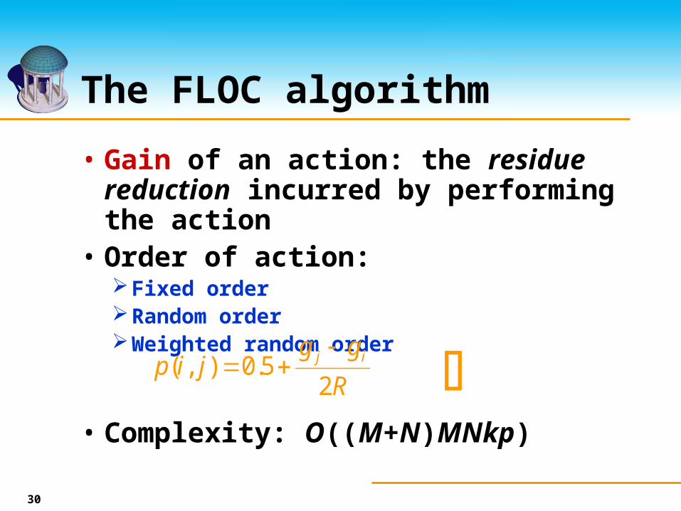
The FLOC algorithm

• Gain of an action: the residue reduction incurred by performing the action

• Order of action:Fixed orderRandom orderWeighted random order

• Complexity: O((M+N)MNkp)

R

ggjip ij

25.0),(

31

The FLOC algorithm

• Additional featuresMaximum allowed overlap among clustersMinimum coverage of clustersMinimum volume of each cluster

• Can be enforced by “temporarily blocking” certain action during the mining process if such action would violate some constraint.

32

Performance

• Microarray data: 2884 genes, 17 conditions100 bi-clusters with smallest residue were

returned.Average residue = 10.34

The average residue of clusters found via the state of the art method in computational biology field is 12.54

The average volume is 25% biggerThe response time is an order of magnitude

faster

33

Conclusion Remark

• The model of bi-cluster is proposed to capture coherent objects with incomplete data set.base residue

• Many additional features can be accommodated (nearly for free).