Beyond Classical Search

C h a p t e r 4

1

(Adapted from Stuart Russel, Dan Klein, and others. Thanks guys!)

2

Outline

•  Hill-climbing

•  Simulated annealing

•  Genetic algorithms (briefly)

•  Local search in continuous spaces (very briefly)

•  Searching with non-deterministic actions

•  Searching with partial observations

•  Online search

Motivation:Typesofproblems

4

LocalSearchAlgorithms

•  So far: our algorithms explore state space methodically •  Keep one or more paths in memory

•  In many optimization problems, path is irrelevant •  the goal state itself is the solution •  State space is large/complex à keeping whole frontier in memory is

impractical

•  Local = Zen = has no idea where it is, just immediate descendants

•  State space = set of “complete” configurations •  A graph of boards, map locations, whatever •  Connected by actions

•  Goal: find optimal configuration (e.g. Traveling Salesman) or, find configuration satisfying constraints, (e.g., timetable)

•  In such cases, can use local search algorithms •  keep a single “current” state, try to improve it •  Constant space, suitable for online as well as offline search

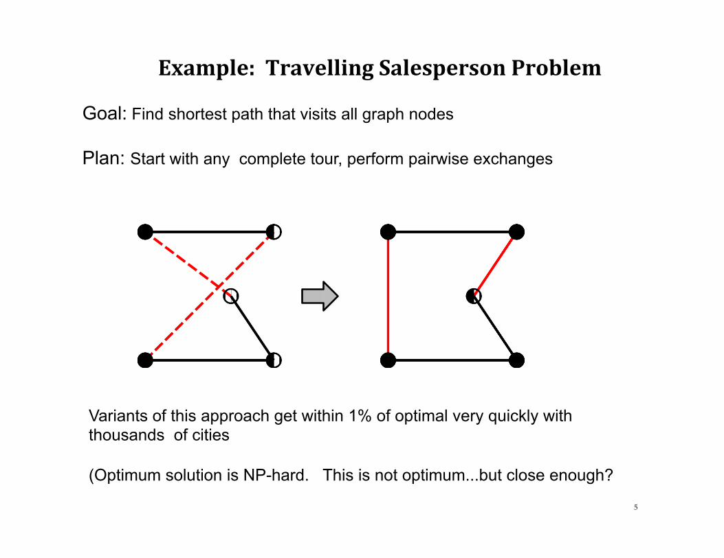
Example:TravellingSalespersonProblem

Goal: Find shortest path that visits all graph nodes Plan: Start with any complete tour, perform pairwise exchanges

Variants of this approach get within 1% of optimal very quickly with thousands of cities (Optimum solution is NP-hard. This is not optimum...but close enough?

5

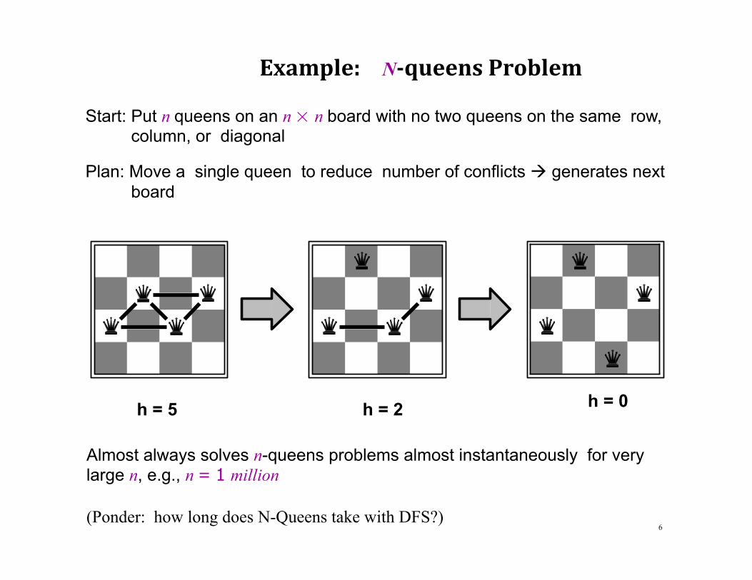
Example: N-queensProblem

Start: Put n queens on an n × n board with no two queens on the same row, column, or diagonal

Plan: Move a single queen to reduce number of conflicts à generates next board

h = 0

6

h = 5 h = 2 Almost always solves n-queens problems almost instantaneously for very large n, e.g., n = 1 million (Ponder: how long does N-Queens take with DFS?)

7

Hill-climbingSearch

“Like climbing Everest ... in thick fog ... with amnesia”

function Hill-Climbing( problem) returns a state that is a local maximum inputs: problem, a problem local variables: current, a node

neighbor, a node

current ← Make-Node(Initial-State[problem]) loop do

neighbor ← a highest-valued successor of current if Value[neighbor] ≤ Value[current] then return State[current] current ← neighbor

end

Plan: From current state, always move to adjacent state with highest value

•  “Value” of state: provided by objective function •  Essentially identical to goal heuristic h(n) from Ch.3

•  Always have just one state in memory!

Hill-climbing:challenges

Useful to consider state space landscape

currentstate

objective function

state space

global maximum

shoulder

local maximum "flat" local maximum

8

“Greedy” nature à can get stuck in:

•  Local maxima

•  Ridges: ascending series but with downhill steps in between

•  Plateau: shoulder or flat area.

Hillclimbing:Gettingunstuck

Pure hill climbing search on 8-queens: gets stuck 86% of time! 14% success

Hill climbing modifications and variants:

•  Allow sideways moves hoping plateau is shoulder, will find uphill gradient - but limit the number of them! (allow 100: 8-queens= 94% success!)

•  Stochastic hill-climbing Choose randomly between uphill successors - choice weighted by steepness of uphill move

•  First-choice: randomly generate successors until find an uphill one - not necessarily the most uphill one à so essentially stochastic too.

•  Random restart: do successive hill-climbing searches - start at random start state each time - guaranteed to find a goal eventually - the most you do, the more chance of optimizing goal

Overall Observation: “greediness” insists on always uphill moves Overall Plan for all variants: Build in ways to allow *some* non-optimal moves

à get out of local maximum and onward to global maximum

10

SimulatedannealingBased metaphorically on metalic annealing Idea: ü  escape local maxima by allowing some random “bad” moves ü  but gradually decrease the degree and frequency ü  à jiggle hard at beginning, then less and less to find global maxima

function Simulated-Annealing( problem, schedule) returns a solution state inputs: problem, a problem

schedule, a mapping from time to “temperature” local variables: current, a node

next, a node T, a “temperature” controlling prob. of downward steps

current ← Make-Node(Initial-State[problem]) for t ← 1 to ∞ do

T ← schedule[t] if T = 0 then return current next ← a randomly selected successor of current ∆E ← Value[next] – Value[current] if ∆E > 0 then current ← next else current ← next only with probability e∆E/T

PropertiesofSimulatedAnnealing

•  Widely used in VLSI layout, airline scheduling, etc.

11

12

Localbeamsearch

Observation: we do have some memory. Why not use it?

Plan: keep k states instead of 1 •  choose top k of all their successors •  Not the same as k searches run in parallel! •  Searches that find good states place more successors in top k

à “recruit" other searches to join them

Problem: quite often, all k states end up on same local maximum Solution: add stochastic element •  choose k successors randomly, biased towards good ones •  note: a fairly close analogy to natural selection (survival of fittest)

Geneticalgorithms

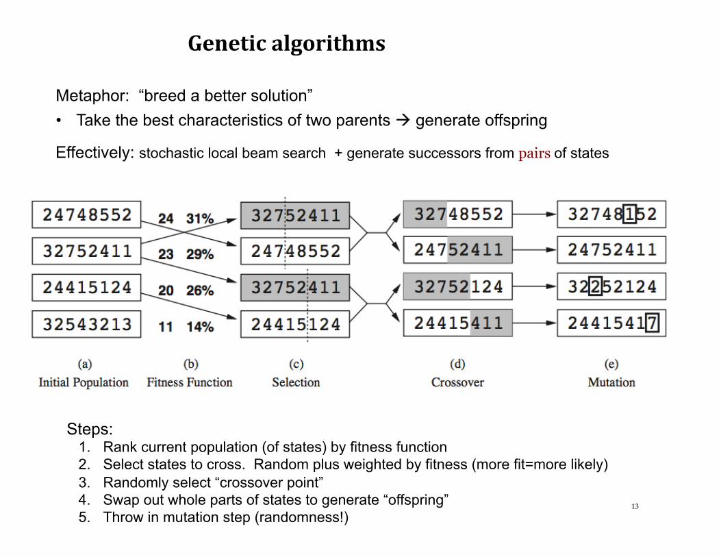
Effectively: stochastic local beam search + generate successors from pairs of states

13

Metaphor: “breed a better solution” •  Take the best characteristics of two parents à generate offspring

Steps: 1.  Rank current population (of states) by fitness function 2.  Select states to cross. Random plus weighted by fitness (more fit=more likely) 3.  Randomly select “crossover point” 4.  Swap out whole parts of states to generate “offspring” 5.  Throw in mutation step (randomness!)

GeneticAlgorithm:N-Queensexample

Geneticalgorithms:analysis

15

Pro: Can jump search around the search space... •  In larger jumps. Successors not just one move away from parents •  In “directed randomness”. Hopefully directed towards “best traits” •  In theory: find goals (or optimum solutions) faster, more likely.

Concerns: Only really works in “certain” situations... •  States must be encodable as strings (to allow swapping pieces) •  Only really works if substrings somehow related functionally meaningful pieces.

à counter-example:

+ = !!!

Overall: Genetic algorithms are a cool, but quite specialized technique •  Depend heavily on careful engineering of state representation •  Much work being done to characterize promising conditions for use.

Searchingincontinuousstate spaces(brieFly...)

16

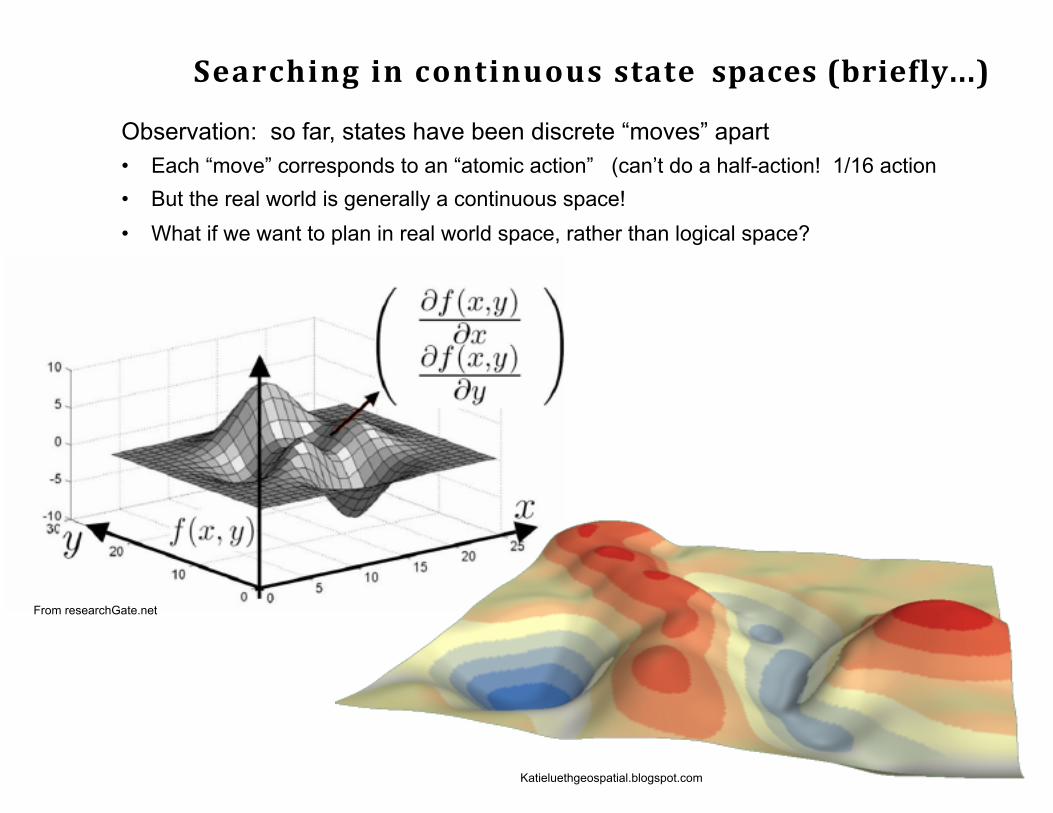
Observation: so far, states have been discrete “moves” apart •  Each “move” corresponds to an “atomic action” (can’t do a half-action! 1/16 action •  But the real world is generally a continuous space! •  What if we want to plan in real world space, rather than logical space?

From researchGate.net

Katieluethgeospatial.blogspot.com

SearchingContinuousspaces

Example: Suppose we want to site three airports in Romania: •  6-D state space defined by (x1, y2), (x2, y2), (x3, y3) •  objective function f (x1, y2, x2, y2, x3, y3) = sum of squared distances from each city

to nearest airport (six dimensional search space)

Approaches: Discretization methods turn continuous space into discrete space •  e.g., empirical gradient search considers ±δ change in each coordinate •  If you make δ small enough, you get needed accuracy

Gradient methods actually compute a gradient vector as a continuous fn.

∇ f = ⎜ ⎜

∂ f ∂ f ∂ f , , , , ,

⎛ ∂ f ∂ f ∂ f ⎞ ⎟ ⎟

⎝ ∂x1 ∂y1 ∂x2 ∂y2 ∂x3 ∂y3 ⎠

to increase/reduce f , e.g., by x ← x + α∇ f (x)

Summary: interesting area, highly complex

Searching with Non-deterministic actions

•  So far: fully-observable, deterministic worlds. –  Agent knows exact state. All actions always produce one outcome. –  Unrealistic?

•  Real world = partially observable, non-deterministic –  Percepts become useful: can tell agent which action occurred

–  Goal: not a simple action sequence, but contingency plan

•  Example: Vacuum world, v2.0 –  Suck(p1, dirty)= (p1,clean)

and sometimes (p2, clean) –  Suck(p1, clean)= sometimes (p1,dirty)

–  If start state=1, solution= [Suck, if(state=5) then [right,suck] ]

AND-OR trees to represent non-determinism

•  Need a different kind of search tree –  When search agent chooses an action: OR node

•  Agent can specifically choose one action or another to include in plan. •  In Ch3 : trees with only OR nodes.

–  Non-deterministic action= there may be several possible outcomes •  Plan being developed must cover all possible outcomes •  AND node: because must plan down all branches too.

•  Search space is an AND-OR tree –  Alternating OR and AND layers –  Find solution= search this tree using same methods from Ch3.

•  Solution in a non-deterministic search space –  Not simple action sequence –  Solution= subtree within search tree with:

•  Goal node at each leaf (plan covers all contingencies) •  One action at each OR node •  A branch at AND nodes, representing all possible outcomes

•  Execution of a solution = essentially “action, case-stmt, action, case-sttmt”.

Non-deterministic search trees

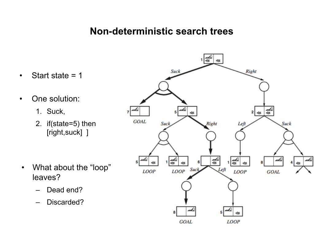
•  Start state = 1

•  One solution: 1.  Suck,

2.  if(state=5) then [right,suck] ]

•  What about the “loop”

leaves? –  Dead end?

–  Discarded?

Non-determinism: Actions that fail

•  Action failure is often a non-deterministic outcome –  Creates a cycle in the search tree

•  If no successful solution (plan) without a cycle: –  May return a solution that contains a

cycle

–  Represents retrying the action

•  Infinite loop in plan execution? –  Depends on environment

•  Action guaranteed to succeed eventually?

–  In practice: can limit loops •  Plan no longer complete (could fail)

Searching with Partial Observations

•  Previously: Percept gives full picture of state –  eg. Whole chess board, whole boggle board, entire robot maze

•  Partial Observation: incomplete glimpse of current state –  Agent’s percept: zero <= percept < full state –  Consequence: we don’t always know exactly what state we’re in.

•  Concept of believe state –  set of all possible states agent could be in.

•  Find a solution (action sequence) that the leads to goal –  Actions applied to a believe state à new believe state based on union of that

action applied to all real states within believe state

Conformant (sensorless) search

•  Worst possible case: percept= null. Blind! –  Actually quite useful: finds plan that works regardless of sensor failure

•  Plan: –  Build a belief state space based on the real state space –  Search that state space using the usual search techniques!

•  Belief state space: –  Believe states: Power-set(real states).

•  Huge! All possible combinations! N physical states = 2N believe states! •  Usually: only small subset actually reachable!

–  Initial State: All states in world •  No sensor input = no idea what state I’m really in. •  So I “believe” I might be in any of them.

Conformant (sensorless) search

•  Belief state space (cont.): –  Actions: basically same actions as in physical space.

•  For simplicity: Assume that illegal actions have no effect •  Example: Move(left, p1) = p1 if p1 is the left edge of the board. •  Can adapt for contexts in which illegal actions are fatal (more complex).

–  Transitions (applying actions): •  Essentially take Union of action applied to all physical states in belief state •  Example: b={s1,s2,s3), then action(b) = Union( action(s1), action(s2),action(s3) ) •  If non-deterministic actions: just Union the set of states that each action produces.

–  Goal Test: Plan must work regardless! •  Believe state is goal iff all physical states it contains are goals!

–  Path cost: tricky •  What if a given action has different costs of different physical states? •  Assume for now: all actions = same cost in all physical states.

•  With this framework: –  can *automatically* construct belief space from any physical space –  Now simply search belief space using standard algos.

Conformant (sensorless) search: Example space

•  Belief state space for the super simple vacuum world •  Observations:

–  Only 12 reachable states. Versus 28= 256 possible belief states –  State space still gets huge very fast! à seldom feasible in practice –  We need sensors! à Reduce state space greatly!

Start!

Goalstates

Searching with Observations (percepts)

•  Obviously: must state what percepts are available

–  Specify what part of “state” is observable at each percept

–  Ex: Vacuum knows position in room, plus if local square dirty •  But no info about rest of squares/space. •  In state 1, Percept = [A, dirty] •  If sensing non-deterministic à could return a set of possible percepts à

multiple possible belief states

•  So now transitions are: –  Predict: apply action to each physical

states in belief state to get new belief state

•  Like sensorless –  Observe: gather percept

•  Or percepts, if non-det. –  Update: filter belief state based on

percepts

Example: partial percepts

•  Initial percept = [A, dirty] •  Partial observation = partial certainty

–  Percept could have been produced by several states (1...or 3) –  Predict: Apply Action à new belief state –  Observe: Consider possible percepts in new b-state –  Update: New percepts then prune belief space

•  Percepts (may) rule out some physical states in the belief state. •  Generates successor options in tree

–  Look! Updated belief states no larger than parents!! •  Observations can only help reduce uncertainty à much better than sensorless state

space explosion!

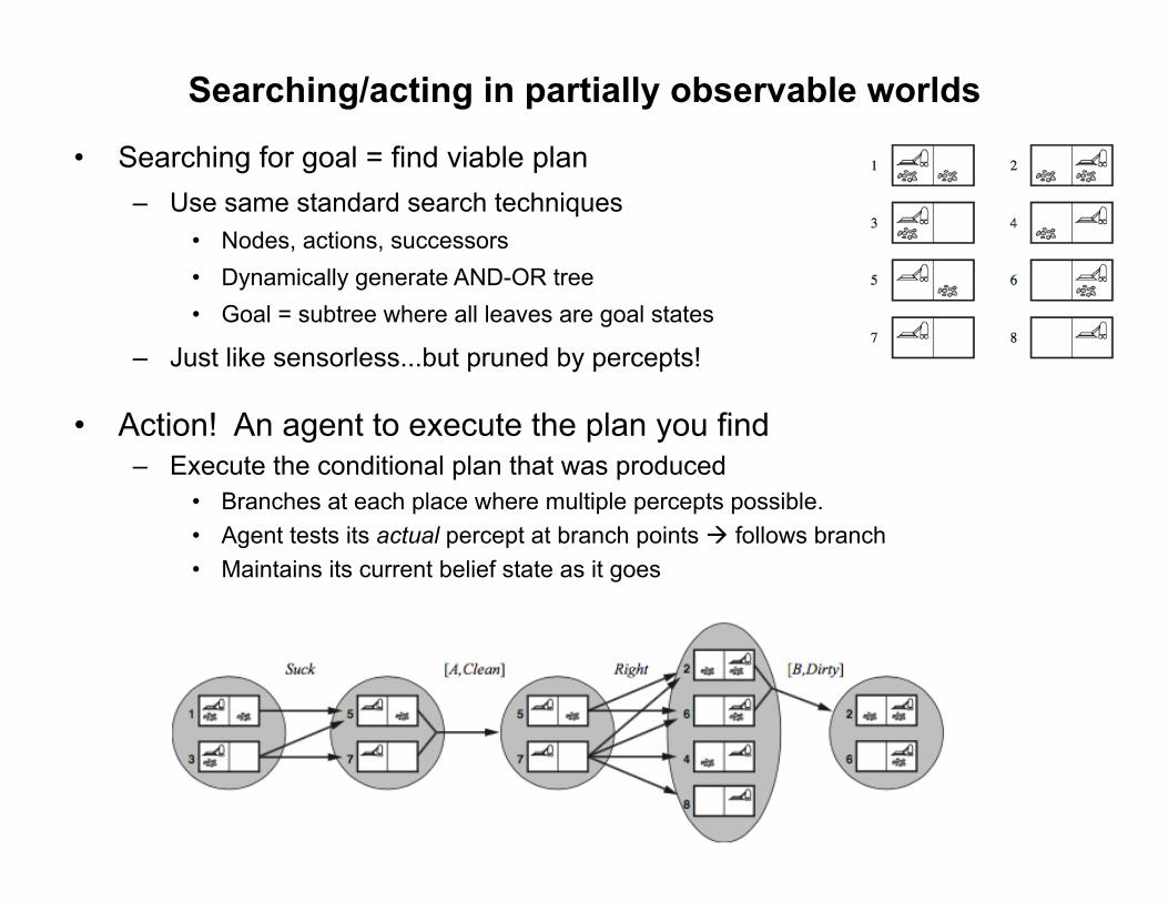
Searching/acting in partially observable worlds

•  Action! An agent to execute the plan you find –  Execute the conditional plan that was produced

•  Branches at each place where multiple percepts possible. •  Agent tests its actual percept at branch points à follows branch •  Maintains its current belief state as it goes

•  Searching for goal = find viable plan –  Use same standard search techniques

•  Nodes, actions, successors •  Dynamically generate AND-OR tree •  Goal = subtree where all leaves are goal states

–  Just like sensorless...but pruned by percepts!

Online Search

•  So far: Considered “offline” search problem –  Works “offline” à searches to compute a whole plan...before ever acting –  Even with percepts à gets HUGE fast in real world

•  Lots of possible actions, lots of possible percepts...plus non-det.

•  Online search –  Idea: Search as you go. Interleave search + action

–  Pro: actual percepts prune huge subtrees of search space @ each move –  Con: plan ahead less à don’t foresee problems

•  Best case = wasted effort. Reverse actions and re-plan •  Worst case: not reversible actions. Stuck!

•  Online search only possible method in some worlds –  Agent doesn’t know what states exist (exploration problem)

–  Agent doesn’t know what effect actions have (discovery learning) –  Possibly: do online search for awhile

•  until learn enough to do more predictive search

The nature of active online search

•  Executing online search = algorithm for planning/acting –  Very different than offline search algos! –  Offline: search virtually for a plan in constructed search space...

•  Can use any search algorithm, e.g., A* with strong h(n) •  A* can expand any node it wants on the frontier (jump around)

–  Online agent: Agent literally is in some place! •  Agent is at one node (state) on frontier of search tree •  Can’t just jump around to other states...must plan from current state. •  (Modified) Depth first algorithms are ideal candidates!

–  Heuristic functions remain critical! •  H(n) tells depth first which of the successors to explore! •  Admissibility remains relevant too: want to explore likely optimal paths first •  Real agent = real results. At some point I find the goal

–  Can compare actual path cost to that predicted at each state by H(n) –  Competitive Ratio: Actual path cost/predicted cost. Lower is better. –  Could also be basis for developing (learning!) improved H(n) over time.

Online Local Search for Agents

•  What if search space is very bushy? –  Even IDS version of depth-first are too costly –  Tight time constraints could also limit search time

•  Can use our other tool for local search! –  Hill-climbing (and variants)

•  Problem: agents in in the physical world, operating –  Random restart methods for avoiding local minima are problematic

•  Can’t just move robot back to start all the time!

–  Random Walk approaches (highly stochastic hill-climbing) can work

–  Will eventually wander across the goal place/state.

•  Random walk + memory can be helpful –  Chooses random moves but…

–  remembers where it’s been, and updates costs along the way –  Effect: can “rock” its way out of local minima to continue search

Online Local Search for Agents

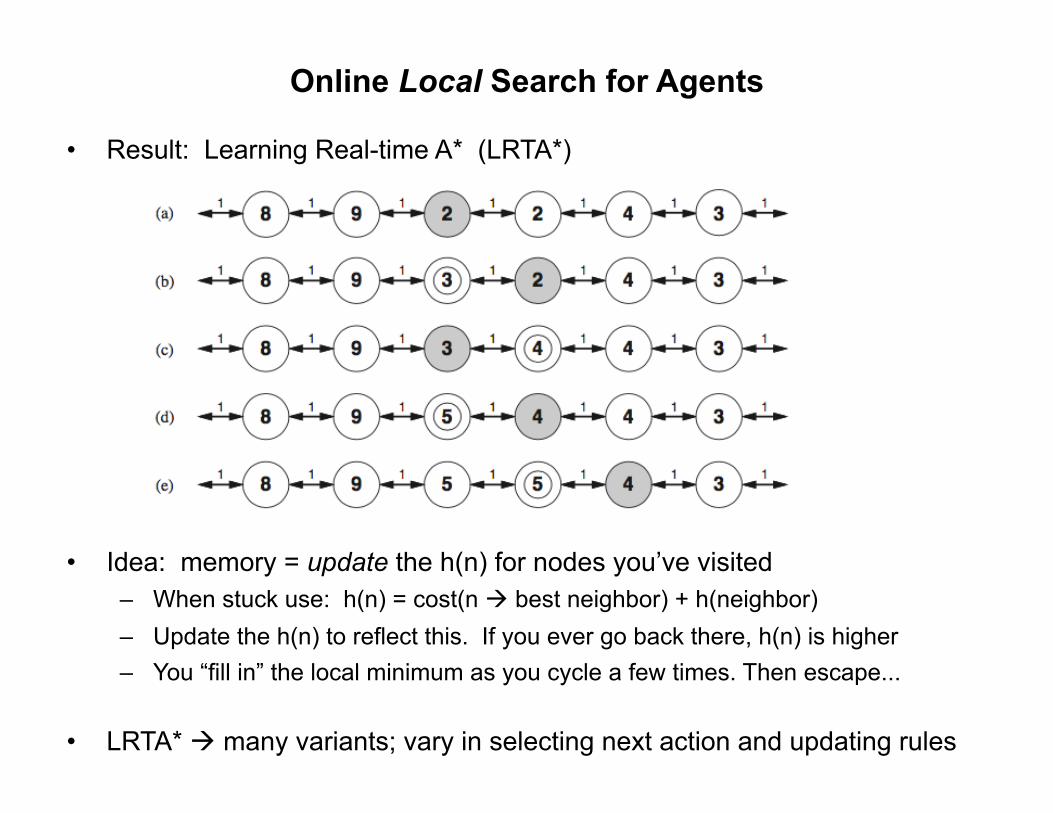
•  Result: Learning Real-time A* (LRTA*)

•  Idea: memory = update the h(n) for nodes you’ve visited –  When stuck use: h(n) = cost(n à best neighbor) + h(neighbor) –  Update the h(n) to reflect this. If you ever go back there, h(n) is higher –  You “fill in” the local minimum as you cycle a few times. Then escape...

•  LRTA* à many variants; vary in selecting next action and updating rules

Chapter 4: Summary

•  Search techniques from Ch.3 –  still form basic foundation for possible search variants –  Are not well-suited directly to many real-world problems

•  Pure size and bushiness of search spaces •  Non-determinism. In Action outcomes. In Sensor reliability. •  Partial observability. Can see all features of current state.

•  Classic search must be adapted and modified for the real world –  Hill-climbing: can be seen as DFS + h(n) ... with depth limit of one. –  Beam search: can be seen as Best First...with Frontier queue limit = k.

–  Stochastic techniques (incl. simulated annealing) = seen as Best-first with weighted randomized Q selection.

–  Belief State Search = identical to normal search...only searching belief space –  Online Search: Applied DFS or local searching

•  With high cost of backtracking and becoming stuck •  Pruning by moving before complete plans made.