Beyond CES: Three Alternative Classes of Flexible ...

©Kiminori Matsuyama and Philip Ushchev, Three Alternative Classes

of 37

Beyond CES: Three Alternative Classes of Flexible Homothetic Demand Systems

Kiminori Matsuyama1 Philip Ushchev2

December 19, 2017, Keio University December 20. 2017, University of Tokyo

1 Department of Economics, Northwestern University, Evanston, USA. Email: [email protected]

2 National Research University Higher School of Economics, Russian Federation. Email: [email protected]


of 37

Homothetic preferences: A general case Common across many fields of applied general equilibrium,

preferences are homothetic and technologies are CRS A preference ≿ over ℝ is called homothetic if any two

indifference sets can be mapped one into the other by a uniform rescaling

Thedirectutilityfunction푢(퐱)is푙푖푛푒푎푟ℎ표푚표푔푒푛푒표푢푠 Theindirectutility푉(퐩,ℎ)canberepresentedas

푉(퐩,ℎ) ≡ 푚푎푥퐱∈ℝ

{푢(퐱)|퐩퐱 ≤ ℎ} =ℎ

푃(퐩)

o ℎ is consumer’s income o 푃(퐩) is an ideal price index


of 37

Homothetic demands and elasticities; A general case The demand system associated with 푃(퐩):

푥 =ℎ푝ℰ (푃)

The inverse demand system associated with 푢(퐱):

푝 =ℎ푥ℰ (푢)

ℰ (푃) and ℰ (푢) are the elasticities defined by:

ℰ (푃) ≡휕푃휕푝

푝푃

, ℰ (푢) ≡휕푢휕푥

푥푢


of 37

Why are homothetic preferences and CRS technologies important?

Under identical homothetic preferences, aggregate consumption

behavior is derived from utility maximization of a representative consumer, even though incomes may vary across households

Perfect competition is valid only when the industry has CRS technologies

Simple behavior of budget shares: o holding the prices constant, the budget share of each good (or factor) is independent

of the household expenditure (or the scale of operation by industries) o this allows us to focus on the role of relative prices in the allocation of resources

Ensure the existence of a balanced growth path in multi-sector growth

models


of 37

CES and its restrictive features In practice, most models assume that preferences/technologies also satisfy constant-elasticity-of-substitution (CES) property, which implies that the price elasticity of demand for each good/factor is constant and identical

across goods/factors relative demand for any two goods/factors is independent of the prices of any

other goods/factors the marginal rate of substitution between any two goods is independent of the

consumption of any other goods in the case of gross substitutes (complements) all goods are inessential

(essential) in a monopolistically competitive setting, each firm sells its product at a

markup independent of the market environment


of 37

Our paper In this paper, we characterize three alternative classes of flexible

homothetic demand systems In each of the three classes, the demand system only depends on

one or two price aggregators for any number of goods Each of these classes contains CES as a special case Yet, they offer three alternative ways of departing from CES,

because non-CES demand systems in these three classes do not overlap

Each of these three classes is flexible in the sense that they are

defined non-parametrically


of 37


of 37

Homothetic demand systems

with a single aggregator (HSA)


of 37

HSA demand systems

Consider a mapping 풔(풛) = 푠 (푧 ), … , 푠 (푧 ) from ℝ to ℝ , A homothetic demand system with a single aggregator (HSA) is

given by:

푥 =ℎ푝푠

푝퐴(퐩)

, 푖 = 1, … ,푛

where 퐴(퐩) is a common price aggregator defined as a solution to

푠푝퐴

= 1


of 37

Example 1: Cobb-Douglas

Set 푠 (푧 ) = 훼 , where 훼 , … ,훼 are positive constants such that

훼 = 1

In this case, we obtain the Cobb-Douglas demand system 푃(퐩) = 푐 ∏ 푝 , but 퐴(퐩) is indeterminate


of 37

Example 2: CES

We obtain the CES demand system if we set 푠 (푧 ) = 훽 푧

Here 휎 > 0 is the constant elasticity of substitution

The price aggregator 퐴(퐩) is proportional to the ideal price index:

퐴(퐩) = 훽 푝 = 푐푃(퐩).

NB: this need not be true in general!


of 37

Example 2: CES The functions 푠 (푧 ) = 훽 푧 are:

increasing when 0 < 휎 < 1 (the goods are gross complements) decreasing when 휎 > 1 (the goods are gross substitutes) constant when 휎 = 1 (the Cobb-Douglas case)


of 37

Example 2: CES and its restrictive nature Definition: Good 푖 is essential (or indispensable) if 푥 = 0 implies 푢(퐱) = 0

(or equivalently, if 푝 → ∞ implies 푃(퐩) → ∞). Good 푖 is inessential (or dispensable), otherwise. Under CES Each good is inessential if 휎 > 1. A good is essential only if 휎 ≤ 1 CES cannot capture situations when only some goods are

essential: if one good is essential, all goods must be essential The very distinction of a good being essential or inessential is

redundant: gross complements (respectively, substitutes) are always essential (inessential) goods


of 37

Integrability Question What are the restrictions to be imposed on the functions 푠 (∙) for

a “candidate” HSA demand system to be compatible with rational consumer behavior?

The answer is given by the following Proposition


of 37

A characterization of HSA

Proposition 1. Consider a mapping 풔(풛) = 푠 (푧 ), … , 푠 (푧 ) from ℝ to ℝ , which is normalized by ∑ 푠 (1) = 1 and satisfies the conditions:

푧 푠 (푧 ) < 푠 (푧 ), 푠 (푧 )푠 푧 ≥ 0 Then: (i) there exists a unique monotone, convex, continuous and homothetic

preference ≿ over ℝ , such that the candidate HSA demand system associated with 풔(풛) is generated by ≿

(ii) the preference ≿ is described by the following ideal price index

ln푃(퐩) = ln퐴(퐩) +푠 (휉)휉

d휉

/ (퐩)

(iii) when 푛 ≥ 3, 퐴(퐩) = 푐푃(퐩) iff ≿ is a CES preference


of 37

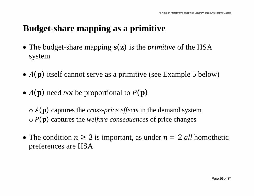
Budget-share mapping as a primitive The budget-share mapping 퐬(퐳) is the primitive of the HSA

system 퐴(퐩) itself cannot serve as a primitive (see Example 5 below) 퐴(퐩) need not be proportional to 푃(퐩) o 퐴(퐩) captures the cross-price effects in the demand system o 푃(퐩) captures the welfare consequences of price changes

The condition 푛 ≥ 3 is important, as under 푛 = 2 all homothetic

preferences are HSA


of 37

Self-duality of the HSA demand systems

Consider a mapping풔∗(풚) = 푠∗(푦 ), … , 푠∗(푦 ) from ℝ to ℝ , The inverse HSA demand system is given by

푝 =ℎ푥푠∗

푥퐴∗(풙)

, 푖 = 1, … ,푛

where 퐴∗(풙) is a common quantity aggregator defined as a solution to

푠∗푥퐴∗

= 1

The two classes of HSA demand systems are self-dual to each other with a one-to-one correspondence between 퐬(퐳) and 퐬∗(퐲), defined by 푠∗ = 푠 (푠∗/푦 )


of 37

Example 3a: Separable translog The translog ideal price index is given by

ln푃(퐩) = 훿 ln 푝 −12

훾 ln푝 ln 푝 − ln 푐,

Here 훿 > 0, while (훾 ) is symmetric and positive semidefinite The following normalizations hold for all 푖 = 1, … , 푛:

훿 = 1, 훾 = 0


of 37

Example 3a: Separable translog In general, the translog demand system is not HSA However, assume additionally the following separability:

훾 =훾훽 (1 − 훽 ), 푖 = 푗−훾훽 훽 , 푖 ≠ 푗 훽 = 1

By setting 푠 (푧 ) = 훿 − 훾훽 ln 푧 , we get:

푥 =ℎ푝푠

푝퐴(풑)

=ℎ푝

훿 − 훾훽 ln푝퐴(풑)


of 37

Example 3a: Separable translog The price aggregator 퐴(퐩) is the weighted geometric mean of

prices:

ln퐴(퐩) = 훽 ln 푝

The price index 푃(퐩) differs from the price aggregator 퐴(퐩):

푃(퐩) = 푐 ⋅ exp 훿 ln푝 −훾2

훽 (ln푝 ) − 훽 ln푝 ≠ 퐴(퐩)


of 37

Example 5: A Hybrid of Cobb-Douglas and CES Consider a convex combination of Cobb-Douglas budget shares

and CES budget shares:

푠 (푧) = 휀훼 + (1 − 휀)훽 푧 Here 0 < 휀 < 1, while 훼 and 훽 are such that

훼 ≥ 0, 훽 > 0, 훼 = 훽 = 1


of 37

Example 5: A Hybrid of Cobb-Douglas and CES The price aggregator 퐴(퐩) is independent of 휀:

퐴(퐩) = 훽 푝

The ideal price index is given by

푃(퐩) = 푐 푝 훽 푝


of 37

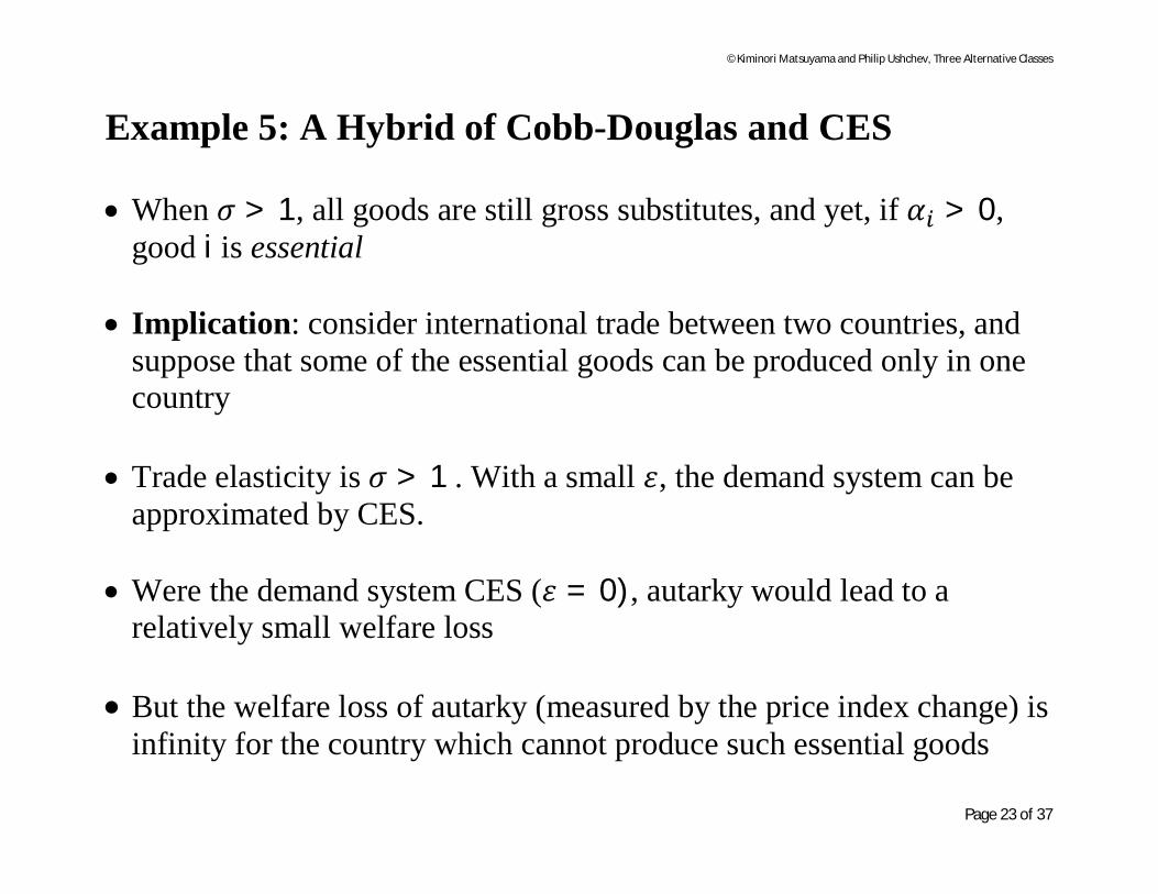
Example 5: A Hybrid of Cobb-Douglas and CES When 휎 > 1, all goods are still gross substitutes, and yet, if 훼 > 0,

good i is essential Implication: consider international trade between two countries, and

suppose that some of the essential goods can be produced only in one country

Trade elasticity is 휎 > 1 . With a small 휀, the demand system can be

approximated by CES. Were the demand system CES (휀 = 0), autarky would lead to a

relatively small welfare loss But the welfare loss of autarky (measured by the price index change) is

infinity for the country which cannot produce such essential goods


of 37

Implicitly additive homothetic

preferences


of 37

HDIA preferences A preference ≿ over ℝ is said to be homothetic with direct

implicit additivity (HDIA) if 푢(퐱) is implicitly defined as a solution to

휙푥푢

= 1

Here the sufficiently differentiable functions 휙 :ℝ → ℝ are o either strictly increasing and strictly concave (goods are gross

substitutes) o or strictly decreasing and strictly convex (goods are gross

complements)

Moreover, 휙 (∙) are normalized as follows: ∑ 휙 (1) = 1


of 37

HDIA preferences Proposition 2. Assume ≿ is a HDIA preference. Then: (i) the Marshallian demands are given by

푥 =ℎ

푃(퐩)(휙 )

푝퐵(퐩)

,

where 푃(푝) is the ideal price index, while 퐵(푝) is another price aggregator:

휙 (휙 )푝퐵

= 1, 푃(푝) = 푝 (휙 )푝퐵(퐩) ;

(ii) when 푛 ≥ 3, we have 퐵(퐩) = 푐푃(퐩) iff ≿ is a CES preference.


of 37

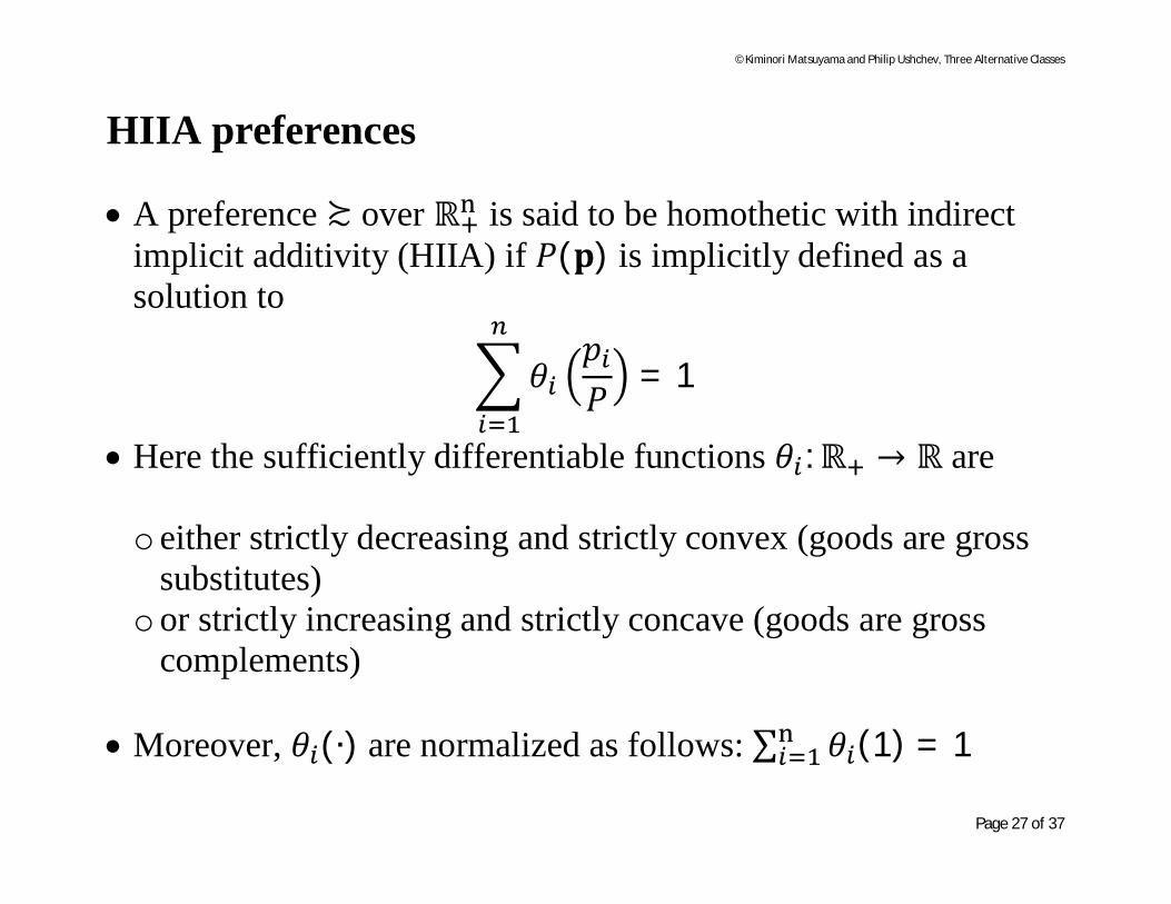
HIIA preferences A preference ≿ over ℝ is said to be homothetic with indirect

implicit additivity (HIIA) if 푃(퐩) is implicitly defined as a solution to

휃푝푃

= 1

Here the sufficiently differentiable functions 휃 :ℝ → ℝ are o either strictly decreasing and strictly convex (goods are gross

substitutes) o or strictly increasing and strictly concave (goods are gross

complements) Moreover, 휃 (∙) are normalized as follows: ∑ 휃 (1) = 1


of 37

HIIA preferences Proposition 3. Assume a preference ≿ is HIIA. Then:

(i) the Marshallian demands are given by

푥 =ℎ

퐶(풑)휃

푝푃(풑)

,

where 푃(풑) is the ideal price index, while 퐶(풑) is another price aggregator:

퐶(풑) ≡ 푝 휃푝푃(풑)

;

(ii) when 푛 ≥ 3, we have 퐶(풑) = 푐푃(풑) iff ≿ is a CES preference.


of 37

Comparing HSA, HDIA, and HIIA


of 37

Three alternative ways of departure from CES Proposition 4. Assume that 푛 ≥ 3. Then: (i) HDIA ∩ HSA = CES; (ii) HIIA ∩ HSA = CES; (iii) HDIA ∩ HIIA = CES.


of 37


of 37

Thank you for your attention!


of 37

HSA are GAS HSA demand systems are the homothetic restriction of what

Pollak (1972) refers to as generalized additively separable (GAS) demand systems

We prefer to call HSA instead of homothetic generalized

additively separable, because it does not nest the demand systems generated by additively separable preferences.

We provide sufficient conditions for the “candidate” HSA demand system to actually be a demand system generated by some continuous and convex homothetic preference


of 37

Example 3b: Modified translog Separable translog is incompatible with gross complementarity To overcome this, consider the following modification:

푠 (푧 ) = max{훿 + 훾훽 ln 푧 , 훾훽 } Here 훿 and 훽 are all positive and such that

훽 = 훿 = 1, 0 < 훾 < min,…,

훿훽


of 37

Example 3b: Modified translog The price aggregator A(퐩) has the same form as under the

separable translog:

ln퐴(퐩) = 훽 ln 푝

The price index 푃(퐩) is given by:

푃(퐩) = 푐 ⋅ exp 훿 ln푝 +훾2

훽 (ln푝 ) − 훽 ln푝 ≠ 퐴(퐩)


of 37

Example 4: Linear expenditure shares Another natural extension of Cobb-Douglas is a demand system

with linear expenditure shares:

푠 (푧 ) = max{(1 − 훿)훼 + 훿훽 푧 , 0} Here δ < 1, 훼 > 0, 훽 > 0, and ∑ 훼 = ∑ 훽 = 1 The goods are o gross complements when 0 < 훿 < 1 o gross substitutes when 훿 < 0


of 37

Example 4: Linear expenditure shares The price aggregator 퐴(퐩) is the weighted arithmetic mean of

prices:

퐴(퐩) = 훽 푝

The ideal price index is given by

푃(퐩) = 푐[퐴(퐩)] 푝 ≠ 퐴(퐩)

Beyond CES: Three Alternative Classes of Flexible ...

Documents

Transcript of Beyond CES: Three Alternative Classes of Flexible ...