Beyond Association Rules: Generalized Rule Discovery Rules/Beyond... · Beyond Association Rules:...

Beyond Association Rules: Generalized Rule Discovery

Geoffrey I. Webb ([email protected])School of Computer Science and Software Engineering,Monash University,Building 26, Melbourne, Victoria 3800 AustraliaTelephone +61 3 9905 3296 Facsimile +61 3 99055146

Songmao Zhang ([email protected])National Library of Medicine (LHC/CgSB)8600 Rockville Pike, MS 43 (Bldg 38A, B1N28T)Bethesda, MD 20894 USA

Abstract. Generalized rule discovery is a rule discovery framework that subsumes association rule discovery and thetype of search employed to find individual rules in classification rule discovery. This new rule discovery framework escapesthe limitations of the support-confidence framework inherent in association rule discovery. This empowers data minersto identify the types of rules that they wish to discover and develop efficient algorithms for discovering those rules. Thispaper presents a scalable algorithm applicable to a wide range of generalized rule discovery task and demonstrates itsefficiency.

Keywords: Rule Discovery, Association Rules, Classification Rules, Rule Search, Pruning Rules

1. Introduction

Rule discovery has evolved within two distinct paradigms. The earliest approaches to rule discov-ery (Buchanan and Feigenbaum, 1978; Michalski, 1977) evolved into the field of classification rulediscovery (Clark and Niblett, 1989; Clearwater and Provost, 1990; Cohen, 1995; Segal and Etzioni,1994; Webb, 1995). Work in affinity analysis led to the development of association rule discoverytechniques (Agrawal et al., 1993; Agrawal and Srikant, 1994; Agrawal et al., 1996). Classificationrule discovery is characterized by a concern for finding highly predictive rules, often using heuristictechniques. Association rule discovery is characterized by complete search to discover all rules thatsatisfy minimum bounds on support (the frequency with which the antecedent and consequent jointlyoccur) and other metrics such as confidence.

Techniques developed in the classification rule discovery paradigm are applicable when the primaryobjective is to obtain a classification capability. They are less useful, however, where the primaryobjective is to increase understanding of a domain by identifying unexpected regularities. Whileclassification learning techniques will identify regularities, they will only identify one type of regularity,antecedents that are highly predictive of a consequent. To use association rule terminology, they arerestricted to finding rules with very high confidence. However, as is well understood in the associationrule community, predictiveness is not a universal measure of how interesting a rule is likely to be(Piatetsky-Shapiro, 1991). The interestingness of a rule will often be a function of both the strengthof the correlation between the antecedent and the consequent and the expected strength of thatcorrelation if the two were independent. For example, a rule buys lingerie→ buys confectionary withconfidence 0.95 (meaning 95% of customers that buy lingerie also buy confectionary) is unlikely to beof interest if 95% of all customers buy confectionary.

Another deficiency of classification rule discovery techniques when applied to gain insight (asopposed to gain classification capability), is that most classification rule discovery techniques seekto find a small set of rules with high coverage. In this context, the antecedents of the rules that areidentified will not usually substantially overlap. In consequence, where there are alternative rules thatapply to a particular class of records (for example rules that have either pregnant or female in theirantecedents) only one is likely to be generated and presented to the user. Often, however, the relativeinterestingness of these rules will depend upon factors that it is infeasible to capture and representto the data mining system. Hence it is valuable to have both alternatives presented to the user, whois then empowered to select which is of greater interest.

c© 2003 Kluwer Academic Publishers. Printed in the Netherlands.

GRD.tex; 21/03/2003; 13:31; p.1

2 Geoffrey I. Webb & Songmao Zhang

Association rules have a different set of strengths and limitations. They allow the use of interest-ingness metrics that consider the difference between the observed and expected degree of correlationand find all rules that satisfy user defined constraints. However, they are based on the applicationof a minimum support constraint. This constraint is required in order to prune the search space andmake computation feasible. However, support is often not directly related to the interestingness ofthe rule. One example of this is the so called vodka and caviar problem (Cohen et al., 2000). A strongcorrelation between Ketel vodka and Beluga caviar may be of considerable interest (as they are highprofit items and hence the affinity is likely to have high financial implications), even though theyare very low volume items that will have low support. Where support is not directly related to theinterestingness of a rule, the application of a minimum support constraint carries a risk that the mostinteresting rules will not be discovered.

In this paper we provide a general characterization of the rule discovery task that encompassesboth classification and association rule discovery as well as supporting new categories of rule discoveryactivity. We provide an algorithm that supports rule discovery for a large and useful subset of thesegeneralized rule discovery tasks and argue that there is a valuable role for the new types of rulediscovery that this algorithm supports.

2. Association and Classification Rule Discovery

In this section we first provide a high level description of association rule discovery and then outlinesome key characteristics that distinguish classification rule discovery.

2.1. Association Rule Discovery

The association rule discovery task can be characterized as follows.

− A dataset D is a finite set of records, where each record is an element to which we apply Booleanpredicates called conditions.

− An itemset I is a set of conditions. The name itemset derives from association rule discovery’sorigins in market basket analysis where each condition denotes the presence of an item in amarket basket.

− coverset(I) denotes the set of records from a dataset that satisfy itemset I.

− An association rule consists of two conjunctions of conditions called the antecedent and conse-quent. An association rule with antecedent a and consequent c is denoted as a→c.

− the support of an association rule a→c = |coverset(a ∪ c)|/|D|.

− the confidence of an association rule a→c = |coverset(a ∪ c)|/|coverset(a)|.

The task involves finding all association rules that satisfy user defined constraints on minimum supportand confidence with respect to a given dataset.

Most association rule discovery algorithms utilize the frequent itemset strategy as exemplifiedby the Apriori algorithm (Agrawal et al., 1993). The frequent itemset strategy first discovers allfrequent itemsets {I : |coverset(I)|/|D| ≥ min support}, those itemsets whose support exceeds a userdefined threshold min support. Association rules are then generated from these frequent itemsets.This approach is very efficient if there are relatively few frequent itemsets. It is, however, subject toa number of limitations.

1. There may be no natural lower bound on support. Associations with support lower than thenominated min support will not be discovered. Infrequent itemsets may actually be especiallyinteresting for some applications. As illustrated by the vodka and caviar problem, in manyapplications high value transactions are likely to be both relatively infrequent and of great interest.

GRD.tex; 21/03/2003; 13:31; p.2

Generalized Rule Discovery 3

2. Even if there is a natural lower bound on support the analyst may not be able to identify it. Ifmin support is set too high then important associations will be overlooked. If it is set too low thenprocessing may become infeasible. There is no means of determining, even after an analysis hasbeen completed, whether it may have overlooked important associations due to the lower boundon support being set too high.

3. Even when a relevant minimum frequency can be specified, the number of frequent itemsets maybe too large for computation to be feasible. Many datasets are infeasible to process using thefrequent itemset approach with sensible specifications of minimum support (Bayardo, 1998).

4. The frequent itemset approach does not readily admit to techniques for improving efficiency byusing constraints on the properties of rules that cannot be derived directly from the propertiesonly of the antecedent, the consequent, or the union of the antecedent and consequent. Thus,they can readily benefit from a constraint on support (which depends solely on the frequencyof the union of the antecedent and consequent) but cannot readily benefit from a constraint onconfidence (which relates to the relationship between the support of the antecedent and of theunion of the antecedent and the consequent). Where such constraints can be specified, potentialefficiencies are lost.

An extension of the frequent itemset approach allows min support to vary depending upon theitems that an itemset contains (Liu et al., 1999). While this introduces greater flexibility to thefrequent itemset strategy, it does not resolve any of the four issues identified above.

Most research in association rule discovery has sought to improve the efficiency of the frequentitemset discovery process (Agarwal et al., 2000; Han et al., 2000; Savasere et al., 1995; Toivonen, 1996,for example). This has not addressed any of the above problems, except the closed itemset approaches(Pasquier et al., 1999; Pei et al., 2000; Zaki, 2000), which reduce the number of itemsets required,alleviating the problems of point 3, but not addressing 1, 2 or 4.

2.2. Classification Rule Discovery

Whereas the primary objective of association rule discovery is to find rules that are interesting to theuser, the primary objective of classification rule discovery is to find rules that can be used to accuratelyclassify objects. Our work falls within the former category. We wish to find interesting rules. However,to do this we extend techniques developed in the classification rule discovery paradigm.

Classification rule discovery usually employs some variant of the covering algorithm (Clark andNiblett, 1989; Cohen, 1995; Michalski, 1977) to find successive rules of the form a → c, where, incommon with association rules, a is a set of conditions, but, unlike association rules, the consequentc is a single condition, a specification that a record belongs to one of a set of disjoint class values.The covering algorithm repeatedly performs a search to discover a rule that optimizes an objectivefunction with respect to the training examples that have not been covered by a rule discovered so far.

A classification rule usually consists of a conjunction of conditions called the antecedent and asingle condition called the consequent. In keeping with the notation for association rule discovery, weuse a→c to denote a classification rule with antecedent a and consequent c.

The classification rule search task involves finding a single classification rule that optimizes a userdefined objective function with respect to a given dataset. Most classification rule discovery algorithmsperform search through the space of combinations of conditions that may appear in the antecedentseeking the combination that optimize the objective function with respect to a given consequent.

3. Generalized rule discovery

A number of research groups have explored rule discovery paradigms that combine elements of associ-ation and classification rule discovery (Bayardo et al., 2000; Bayardo and Agrawal, 1999; Clearwaterand Provost, 1990; Rymon, 1992). From classification rule discovery they retain the objectives ofsearching for rules that optimize an objective function and that restrict the consequent to a single

GRD.tex; 21/03/2003; 13:31; p.3


condition that represents a value of a single class variable. From association rule discovery theytake the objective of finding multiple rules, abandoning the covering objective, seeking instead manyrules that each individually optimize some objective function. These approaches have advantagesover standard classification and association rule discovery in numerous applications. Unlike standardclassification rule discovery algorithms they return all rules that satisfy the objective function. Thisallows the user to select between these rules on criteria that may be difficult to specify and quantifyin a manner suitable for application by the rule discovery system. Unlike standard association rulediscovery algorithms they do not have to apply a constraint on minimum support. This greatlyincreases their versatility and allows the application solely of objective functions that are directlyapplicable to a particular rule discovery task.

However, these new rule discovery algorithms restrict discovery to rules with a value of a prespec-ified class variable as the consequent, a restriction that limits their applicability in “classical” datamining contexts where users wish to perform a wide ranging exploration for unexpected patterns indata. Having to specify a class variable greatly limits the rules that might be found. It might bethought that the process could simply be repeated for each potential consequent. However, in manydata mining applications there are many thousands of potential consequents and such a strategywould be infeasible.

We propose a new rule discovery paradigm, generalized rule discovery, that combines elementsof classification and association rule discovery as in previous research, but without the requirementthat a class variable be specified. The result is a very general and flexible approach to rule discoverythat can support search for rules that satisfy a wider range of constraints than the minimum supportand confidence constraints of association rule discovery while freeing the discovery task from thelimitations of a prespecified class variable. We maintain that this new paradigm facilitates valuablenew forms of rule discovery.

Note that this differs from approaches to classification rule discovery that use association rulediscovery techniques to find rules for classification (Liu et al., 1998). Rather, we extend algorithmsdeveloped in the classification context to support the same objective as association rule discovery.Our new algorithm is aimed at discovering interesting rules rather than rules for classification.

3.1. Formal Description of Generalized Rule Discovery

A formal definition of the generalized rule discovery task is given in the following.

Definition 1. A generalized rule discovery task (abbreviated as GRDtask) is a 4-tuple 〈A, C,D,M〉and the solution to the generalized rule discovery task is a set of rules each of which takes the formof X→Y , where

A: is a nonempty set of conditions, called antecedent conditions;

C: is a nonempty set of conditions, called consequent conditions;

D: is a nonempty set of records, called the dataset, where for each record d ∈ D, conditions(d) ⊆ A∪C,where conditions(d) is the set of conditions that apply to d. For any set of conditions S ⊆ A∪C,

let coverset(S) = {d|d ∈ D ∧ S ⊆ conditions(d)}, and let cover(S) = |coverset(S)||D| ;

M: is a set of constraints on the rules that form the solution for the generalized rule discovery task.

X: is a nonempty set of conditions, called the antecedent;

Y : is a nonempty set of conditions, called the consequent;

solution : 〈A, C,D,M〉 → {X →Y } is a many-to-one function mapping a GRDtask to its solution,satisfying solution(〈A, C,D,M〉) = {X→Y |X ⊆ A∧ Y ⊆ C ∧X→Y satisfies all constraints inM with respect to D}.

GRD.tex; 21/03/2003; 13:31; p.4


Generalized rule discovery separates the available conditions into two sets, the antecedent condi-tions and the consequent conditions. These specify, respectively, the conditions that may appearin the antecedent or the consequent of a solution to a GRDtask. These two sets may overlap.These are distinguished in the specification of a GRDtask in recognition that in many data miningcontexts some conditions represent factors that may be directly manipulated while others representoutcomes that users would like to influence by manipulation of the first set of conditions. In sucha context the user will be interested in rules where the antecedent is a selection from the first setof conditions and the consequent is a selection from the second set. This is because such rules canbe operationalized. For example, conditions that represent identifiable characteristics of a customermake natural antecedents because they can be manipulated by strategies to acquire customers withspecific profiles or by selecting such customers for a specific action once acquired. Conditions thatrepresent a customer’s propensity to engage in a particular type of action make natural consequents,as it is for their propensity to act that we want to select a particular group.

3.2. Configuration

To emulate association rule discovery, the antecedent conditions and consequent conditions shouldboth be the set of all conditions that appear in the dataset, and the set of constraints M shouldconsist of constraints on the minimum allowed values for support and confidence. To emulate searchfor rules within classification rule discovery, the consequent conditions should be set to the valuesof the class variable, the antecedent conditions should be set to all other conditions, and M shouldconstrain the solution to the rule that optimizes the objective function.

In the current work, however, we utilize a set of constraints that illustrate the manner in whichGRD can support types of rule discovery not supported by other existing rule discovery paradigms.To this end we define four measures with respect to a rule X→Y :

coverage(X →Y ) = cover(X),

support(X→Y ) = cover(X ∪ Y ),

confidence(X →Y ) =support(X→Y )

coverage(X →Y ),

leverage(X →Y ) = support(X→Y ) − cover(X) × cover(Y ).

Piatetsky-Shapiro (1991) argues that many measures of interestingness are based on the differencebetween the observed joint frequency of the antecedent and consequent, support(X → Y ), and thefrequency that would be expected if the two were independent, cover(X)× cover(Y ). He asserts thatthe simplest such measure is one that we call leverage, as defined above. Note that leverage can alsobe expressed as cover(X)×(confidence(X →Y ) − cover(Y )). Expressed in this form, it has also beencalled weighted relative accuracy (Todorovski et al., 2000).

Leverage is of interest because it measures the number of additional records that an interactioninvolves above and beyond those that should be expected if one assumes independence. This directlyrepresents the volume of an effect and hence will often directly relate to the ultimate metric of interestto the user such as the magnitude of the profit associated with the interaction between the antecedentand consequent. This contrasts with the traditional association rule measure

lift(X→Y ) =support(X→Y )

cover(X) × cover(Y )

which is the ratio of the observed frequency with which the consequent occurs in the context ofthe antecedent over that expected if the two were independent. A rule with high lift may be oflittle interest because it applies very infrequently. This might be provided as justification for theapplication of minimum support constraints in conjunction with the lift measure, but this is at best acrude approximate fix to the problem. It results in a step function with the very undesirable propertythat the addition of one more record in support of a rule with very high lift can transform it from

GRD.tex; 21/03/2003; 13:31; p.5


{}

{a}

{b} {a, b}

{c}{a, c}

{b, c} {a, b, c}

{d}

{a, d}

{b, d} {a, b, d}

{c, d}{a, c, d}

{b, c, d} {a, b, c, d}

Figure 1. A fixed-structure search space

being of no interest whatsoever because it fails to meet a minimum support criterion to being of veryhigh interest because it now meets that criterion. In contrast to the use of support and lift as measuresof interest, the use of leverage ensures both that rules with very low support will receive low valuesand that there are no artificial threshold values at which dramatic changes in the objective functionoccur.

With these considerations in mind, for the purposes of this paper we restrict the set of constraintsM to constraints on the coverage, support, confidence, and leverage of a rule. M is composed of

maxRules denoting the maximum number of rules in the solution (which will consist of the ruleswith the highest values for leverage of those that satisfy all other constraints),

maxLHSsize denoting maximum number of conditions allowed on the antecedent of rule

minCoverage denoting the minimum coverage,

minSupport denoting the minimum support,

minConfidence denoting the minimum confidence, and

minLeverage = max(0.0, β(RS,maxRules)), where RS is the set of rules {R|coverage(R) > minCoverage∧support(R) > minSupport ∧ confidence(R) > minConfidence}, and β(Z, n) is the leverage ofthe nth rule in Z sorted from highest to lowest by leverage.

These user configured constraints are augmented by the constraints that the antecedent of a rule iscomposed of at least one condition and the consequent of rule is composed of single condition.

In consequence, in the current work, solution : 〈A, C,D,M〉 → {X→Y } is a many-to-one functionmapping a GRDtask to its solution, satisfying solution(〈A, C,D,M〉) = {X → Y |X ⊆ A ∧ Y ⊆C ∧ 1 6 |X| 6 maxLHSsize ∧ |Y | = 1 ∧ coverage(X →Y ) > minCoverage ∧ support(X →Y ) >

minSuport ∧ confidence(X →Y ) > minConfidence ∧ leverage(X →Y ) > minLeverage}.

4. The OPUS Search Algorithm

We propose an algorithm for solving a useful class of GRD tasks based on the OPUS (Webb, 1995)search algorithm. OPUS provides efficient search for subset selection, such as selecting a subsetof available conditions that optimizes a specified measure. It was developed for classification rulediscovery. Prior to the development of OPUS, classification rule discovery algorithms that performedcomplete search ordered the available conditions and then conducted a systematic search over theordering in such a manner as to guarantee that each subset was investigated once only, as illustratedin Figure 1.

Critical to the efficiency of such search is the ability to identify and prune sections of the searchspace that cannot contain solutions to the search task. This is usually achieved by identifying subsetsthat cannot appear in a solution. For example, it might be determined that no superset of {b} can be

GRD.tex; 21/03/2003; 13:31; p.6


{}

{a}

{b} ×

{c}{a, c}

{b, c} {a, b, c}

{d}

{a, d}

{b, d} {a, b, d}

{c, d}{a, c, d}

{b, c, d} {a, b, c, d}

Figure 2. Pruning a branch from a fixed-structure search space

{}

{a}

{b} ×

{c}{a, c}× ×

{d}

{a, d}× ×

{c, d}{a, c, d}

× ×

Figure 3. Pruning all nodes containing a single condition from a fixed-structure search space

a solution in the search space illustrated in Figure 1. Under previous search algorithms (Clearwaterand Provost, 1990; Morishita and Nakaya, 2000; Provost et al., 1999; Rymon, 1992; Segal and Etzioni,1994), the search space below such a node was pruned, as illustrated in Figure 2. In this example,pruning removes one subset from the search space.

This contrasts with the pruning that would occur if all supersets of the pruned subset were removedfrom the search space, as illustrated in Figure 3. This optimal pruning almost halves the search spacebelow the parent node.

OPUS achieves the pruning illustrated in Figure 3 by maintaining a set of available items at eachnode in the search space. When adding an item i to the current subset s results in a subset s∪{i} thatcan be pruned from the search space, i is simply removed from the set of available items at s whichis propagated below s. As supersets of s ∪ {i} below s can only be explored after s ∪ {i}, this simplemechanism with negligible computational overheads guarantees that no superset of a pruned subsetwill be generated in the search space below the parent of the pruned node. This greatly expands thescope of a pruning operation from that achieved by previous algorithms which only extended to thespace directly beneath the pruned node. Further pruning can be achieved by reordering the searchspace (Webb, 1995). However, this proves to be infeasible in generalized rule discovery search as thereis a large amount of information associated with each node in the search space (specifically, the setof records covered by the current antecedent) and it is more efficient to utilize this information whenit is first calculated than to either store it for later use or recalculate it at a later stage as would berequired if the nodes were reordered before expansion.

Note that nodes are pruned only when they need not be explored during the search. Nodes mayneed to be explored even when they are not candidate solutions because candidate solutions mightoccur deeper in the search space below those nodes. Pruning is applied only when this is not the case.In consequence, OPUS does not require either monotonicity or anti-monotonicity from its objectivefunction. It requires only that the value of the objective function can be bounded so that branch andbound techniques can exclude sections of the search space from exploration.

It is interesting to observe that while the rule discovery systems Max-Miner and Dense-Miner havebeen described as using SE-Tree search (Bayardo, 1998; Bayardo et al., 2000), they are perhaps more

GRD.tex; 21/03/2003; 13:31; p.7


accurately described as using OPUS search, as they use both the propagation of a set of availableitems and search space reordering, two strategies that distinguish OPUS search from SE-Tree search.

5. The GRD Algorithm

The GRD algorithm extends the OPUS search algorithm to generalized rule discovery (Webb, 2000).To simplify the search problem, the consequent of a rule is restricted to a single condition. Rules ofthis restricted form are of interest for many data mining applications, and indeed many associationrule discovery systems also impose such a constraint.

Whereas OPUS supports search through spaces of subsets, the generalized rule discovery taskrequires search through the space of pairs 〈a ⊆ AntecedentConditions, c ∈ ConsequentConditions〉,where a is the antecedent and c the consequent of rule. GRD achieves this by performing OPUS searchthrough the space of antecedents, maintaining at each node a set of potential consequents, each ofwhich is explored at each node.

GRD extends previous algorithms that perform OPUS-like search for rule discovery (Bayardo, 1998;Bayardo et al., 2000) by removing the requirement that the consequent of each of the rules discoveredbe one of the values of a single ‘class’ variable. Unlike Bayardo and Agrawal’s (1999) technique thatfinds all rules that can maximize any of a number of widely used measures of interestingness, GRDfinds all rules that satisfy a specified set of constraints. These may include rules that achieve highscores but not the highest according to the primary measure of interestingness. We believe that thisis important, as it is often not possible for the user to provide formal measures of all criteria thatrelate to the degree of interestingness of a rule. It can be valuable for the user to be provided witha range of alternative rules that score highly on the specified interestingness measure, in order thatthey can then apply further criteria to select the rules of greatest interest, such as the feasibility ofoperationalizing business plans based on a rule.

The algorithm relies upon there being a set of user defined constraints on the acceptable rules.These are used to prune the search space. Such constraints can take many forms, ranging from thetraditional association rule discovery constraints on support and confidence to a constraint that onlythe n rules that maximize some statistic be returned. The solution to a GRDtask is the set of rulesthat satisfy all the constraints. Note that it may not be apparent when a rule is encountered whetheror not it is in the solution. For example, if we are seeking the 100 rules with the highest leverage, wemay not know the cutoff value for leverage until the search has been completed.

To manage this problem, GRD is restricted to GRDtasks 〈A, C,D,M〉 that satisfy the followingproperty:

∀R ⊆ {W →Z |W ⊆ A∧ Z ⊆ C},

solution(〈A, C,D,M〉) ∩ R ⊆ solution(〈A, C,D,M∧ X→Y ∈ R〉)) (1)

This allows an incremental search to be performed. In this search, rules in the search space areconsidered one at a time. Let S represent the set of rules in the search space explored so far. A recordcurrentSolution is maintained such that currentSolution = solution(〈A, C,D,M ∧ X → Y ∈ S〉).For each new rule r considered during the search, the algorithm need only update currentSolutionby

− adding r if r ∈ solution(〈A, C,D,M∧ X→Y ∈ S ∪ {r}〉), and

− removing any z ∈ currentSolution if z 6∈ solution(〈A, C,D,M∧ X→Y ∈ S ∪ {r}〉).

Appendix A presents a proof that the update strategy for currentSolution is sufficient andnecessary to ensure that on termination currentSolution = solution(〈A, C,D,M〉).

This simple constraint, (1), greatly simplifies the search task. The constraint is not unduly re-strictive as it is satisfied by all M that we have considered to date. Note in particular that it allowsmonotone and anti-monotone constraints, as well as constraints that are neither. Our algorithm usesbranch-and-bound techniques, and hence relies on neither monotonicity nor anti-monotonicity in its

GRD.tex; 21/03/2003; 13:31; p.8


constraints. The objective function, leverage, used in our experiments is non-monotone. The additionof a new condition to an antecedent can raise, lower or leave unaffected the leverage of a rule.

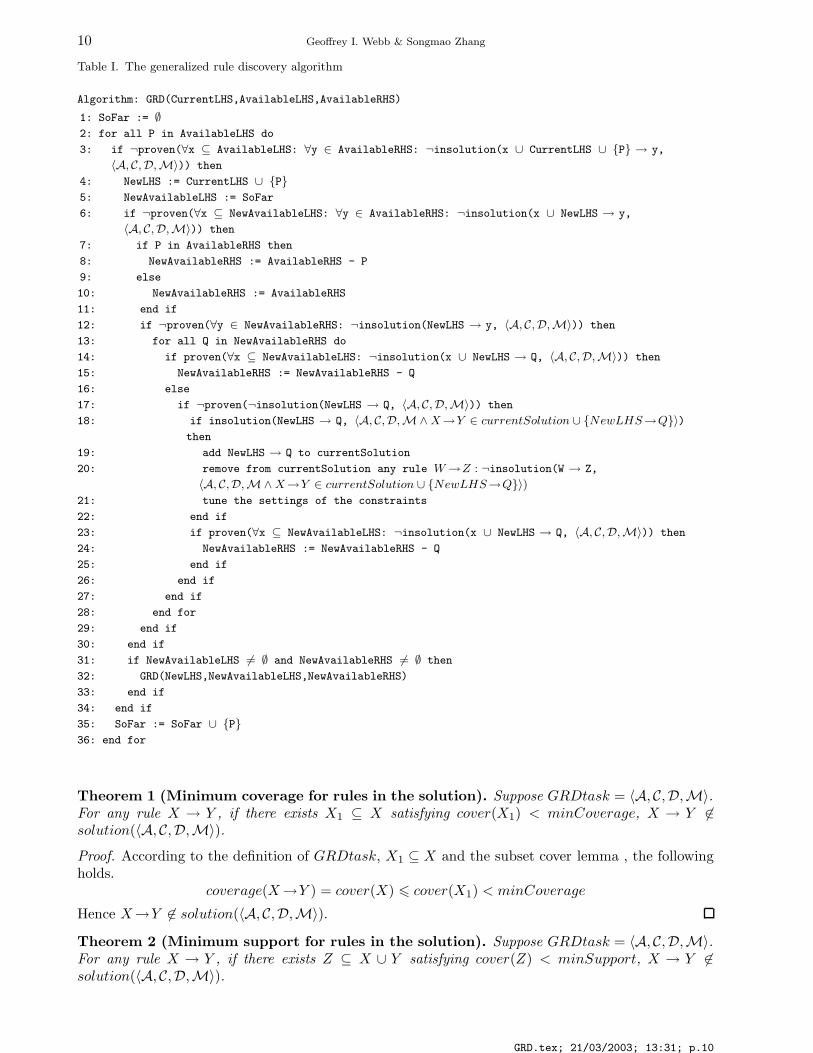
Table I displays the algorithm that results from extending the OPUS search algorithm (Webb,1995) to obtain efficient search for this rule discovery task. The algorithm is presented as a recursiveprocedure with three arguments:

CurrentLHS: the set of conditions in the antecedent of the rule currently being considered.

AvailableLHS: the set of conditions that may be added to the antecedent of rules to be exploredbelow this point

AvailableRHS: the set of conditions that may appear on the consequent of a rule in the searchspace at this point and below

The algorithm also maintains a global variable currentSolution, the solution to GRDtask constrainedto the rules in the search space considered so far.

To solve GRDtask 〈A, C,D,M〉, currentSolution is initialized to ∅ and the initial call to GRD ismade with CurrentLHS=∅, AvailableLHS=A, and AvailableRHS=C.

The GRD algorithm is a search procedure that starts with rules with one condition in the an-tecedent and searches through successive rules formed by adding conditions to the antecedent. Itloops through each condition in AvailableLHS and adds it to CurrentLHS to form the NewLHS. Forthe NewLHS, it loops through each condition c in AvailableRHS to check whether NewLHS →{c}might be in the solution. After the AvailableRHS loop, the procedure is recursively called with thearguments NewLHS, NewAvailableLHS and NewAvailableRHS. The two latter arguments are formedby removing the pruned conditions from AvailableLHS and AvailableRHS, respectively.

Pruning rules seek to identify areas of the search space that cannot contain a solution. This isrepresented within the algorithm by the use of a predicate insolution(a → c, T ) that is true iff therule a→ c is in the solution to the GRDtask, T . The predicate proven(X) is true iff pruning rulesprovided to the algorithm prove the proposition X. The use of this predicate allows us to abstractthe algorithm from the sets of pruning rules that might be used to provide efficient search for a givenset of constraints. The efficiency of GRD will depend critically on the power of the pruning rules withwhich it is provided.

As GRD traverses the space of rules, the minLeverage constraint is increased dynamically so thatit is always the maxRulesth leverage value of all the rules searched so far. Line 19 records the rulessatisfying the current constraints. Whenever adding a rule to currentSolution causes the number ofrules in currentSolution to exceed maxRules, Line 20 removes the unqualified rule whose leveragevalue ranks (maxRules + 1). When the search is finished, currentSolution is the solution to theGRDtask.

Appendix B proves the correctness of the GRD′ algorithm, a variant of GRD with all pruningremoved. In the following section, we will list the pruning techniques adopted in GRD. Their correct-ness lies in the theorems on properties of rules in the solution and relations between rules. As GRD ′

is correct, GRD will also be correct so long as all the pruning rules are correct.

6. Pruning in Search for Rules

6.1. Properties of the rules in the solution of GRDtask

To facilitate the analysis of the GRD algorithm, we analyze some necessary properties of GRDtasksand their solutions. Before presenting the theorems, we give the following lemma.

Lemma 1 (Subset cover). Suppose GRDtask = 〈A, C,D,M〉. For any S1, S2 ⊆ A∪C, if S1 ⊆ S2,then coverset(S2) ⊆ coverset(S1), and hence, cover(S2) 6 cover(S1) holds.

Proof. For any d ∈ coverset(S2), according to the definition of GRDtask, S2 ⊆ conditions(d) holds.Since S1 ⊆ S2, S1 ⊆ conditions(d) holds. Hence d ∈ coverset(S1). So coverset(S2) ⊆ coverset(S1)holds.

GRD.tex; 21/03/2003; 13:31; p.9


Table I. The generalized rule discovery algorithm

Algorithm: GRD(CurrentLHS,AvailableLHS,AvailableRHS)

1: SoFar := ∅

2: for all P in AvailableLHS do

3: if ¬proven(∀x ⊆ AvailableLHS: ∀y ∈ AvailableRHS: ¬insolution(x ∪ CurrentLHS ∪ {P} → y,

〈A, C,D,M〉)) then

4: NewLHS := CurrentLHS ∪ {P}

5: NewAvailableLHS := SoFar

6: if ¬proven(∀x ⊆ NewAvailableLHS: ∀y ∈ AvailableRHS: ¬insolution(x ∪ NewLHS → y,

〈A, C,D,M〉)) then

7: if P in AvailableRHS then

8: NewAvailableRHS := AvailableRHS - P

9: else

10: NewAvailableRHS := AvailableRHS

11: end if

12: if ¬proven(∀y ∈ NewAvailableRHS: ¬insolution(NewLHS → y, 〈A, C,D,M〉)) then

13: for all Q in NewAvailableRHS do

14: if proven(∀x ⊆ NewAvailableLHS: ¬insolution(x ∪ NewLHS → Q, 〈A, C,D,M〉)) then

15: NewAvailableRHS := NewAvailableRHS - Q

16: else

17: if ¬proven(¬insolution(NewLHS → Q, 〈A, C,D,M〉)) then

18: if insolution(NewLHS → Q, 〈A, C,D,M∧ X→Y ∈ currentSolution ∪ {NewLHS→Q}〉)

then

19: add NewLHS → Q to currentSolution

20: remove from currentSolution any rule W →Z : ¬insolution(W → Z,

〈A, C,D,M∧ X→Y ∈ currentSolution ∪ {NewLHS→Q}〉)

21: tune the settings of the constraints

22: end if

23: if proven(∀x ⊆ NewAvailableLHS: ¬insolution(x ∪ NewLHS → Q, 〈A, C,D,M〉)) then

24: NewAvailableRHS := NewAvailableRHS - Q

25: end if

26: end if

27: end if

28: end for

29: end if

30: end if

31: if NewAvailableLHS 6= ∅ and NewAvailableRHS 6= ∅ then

32: GRD(NewLHS,NewAvailableLHS,NewAvailableRHS)

33: end if

34: end if

35: SoFar := SoFar ∪ {P}

36: end for

Theorem 1 (Minimum coverage for rules in the solution). Suppose GRDtask = 〈A, C,D,M〉.For any rule X → Y , if there exists X1 ⊆ X satisfying cover(X1) < minCoverage, X → Y 6∈solution(〈A, C,D,M〉).

Proof. According to the definition of GRDtask, X1 ⊆ X and the subset cover lemma , the followingholds.

coverage(X →Y ) = cover(X) 6 cover(X1) < minCoverage

Hence X→Y 6∈ solution(〈A, C,D,M〉).

Theorem 2 (Minimum support for rules in the solution). Suppose GRDtask = 〈A, C,D,M〉.For any rule X → Y , if there exists Z ⊆ X ∪ Y satisfying cover(Z) < minSupport, X → Y 6∈solution(〈A, C,D,M〉).

GRD.tex; 21/03/2003; 13:31; p.10


Proof. According to the definition of GRDtask, Z ⊆ X∪Y and the subset cover lemma, the followingholds.

support(X→Y ) = cover(X ∪ Y ) 6 cover(Z) < minSupport

Hence X→Y 6∈ solution(〈A, C,D,M〉).

Theorem 3 (Minimum leverage for rules in the solution). Suppose GRDtask = 〈A, C,D,M〉.

For any rule X → Y , if cover(Y ) > 1 − minLeveragecover(X) or cover(X) > 1 − minLeverage

cover(Y ) , X → Y 6∈

solution(〈A, C,D,M〉).

Proof. Let us first prove the theorem when cover(Y ) > 1 − minLeveragecover(X) . According to the definition

of GRDtask, we obtain:

leverage(X →Y ) = support(X→Y )− cover(X) × cover(Y ) = cover(X ∪ Y ) − cover(X) × cover(Y )

From cover(Y ) > 1 − minLeveragecover(X) we obtain cover(X) × cover(Y ) > cover(X) − minLeverage, thus

leverage(X →Y ) satisfies:

leverage(X →Y ) < cover(X∪Y )−(cover(X)−minLeverage) = cover(X∪Y )−cover(X)+minLeverage

From the subset cover lemma we obtain cover(X ∪ Y ) 6 cover(X). Thus the following holds.

leverage(X →Y ) < minLeverage

Hence X → Y 6∈ solution(〈A, C,D,M〉). Similarly the theorem is proved when cover(X) > 1 −minLeverage

cover(Y ) .

Theorem 4 (Minimum leverage for the antecedent of rules in the solution). SupposeGRDtask = 〈A, C,D,M〉. For any rule X → Y , if cover(X) × (1 − cover(X)) < minLeverage,X→Y 6∈ solution(〈A, C,D,M〉).

Proof. Firstly let us assume cover(X) 6 cover(Y ). Thus 1−cover(X) > 1−cover(Y ) holds. Accordingto the definition of GRDtask and the subset cover lemma, we obtain:

leverage(X →Y ) = support(X→Y ) − cover(X) × cover(Y ) = cover(X ∪ Y ) − cover(X) × cover(Y )

6 cover(X) − cover(X) × cover(Y ) = cover(X) × (1 − cover(Y ))

6 cover(X) × (1 − cover(X)) < minLeverage

Secondly let us assume cover(X) > cover(Y ). Thus cover(Y )cover(X) < 1 holds. According to the definition

of GRDtask and the subset cover lemma, we obtain:

leverage(X →Y ) = support(X→Y ) − cover(X) × cover(Y ) = cover(X ∪ Y ) − cover(X) × cover(Y )

6 cover(Y ) − cover(X) × cover(Y ) = cover(Y ) × (1 − cover(X))

< cover(Y ) ×minLeverage

cover(X)< minLeverage

So for both cases leverage(X →Y ) < minLeverage holds. Hence X→Y 6∈ solution(〈A, C,D,M〉).

Theorem 5 (Minimum confidence for rules in the solution). Suppose GRDtask =

〈A, C,D,M〉. For any rule X→Y , if cover(Y )cover(X) < minConfidence, X→Y 6∈ solution(〈A, C,D,M〉).

Proof. According to the definition of GRDtask and the subset cover lemma, we obtain:

confidence(X→Y ) =support(X→Y )

coverage(X →Y )=

cover(X ∪ Y )

cover(X)6

cover(Y )

cover(X)

From cover(Y )cover(X) < minConfidence, confidence(X → Y ) < minConfidence holds. Hence, X → Y 6∈

solution(〈A, C,D,M〉).

GRD.tex; 21/03/2003; 13:31; p.11


Theorem 6 (Full cover). Suppose GRDtask = 〈A, C,D,M〉. For any rule X→Y , if cover(X) = 1or cover(Y ) = 1, leverage(X →Y ) = 0 holds.

Proof. When cover(X) = 1, cover(X ∪ Y ) = cover(Y ) holds. Thus the following holds.

leverage(X →Y ) = support(X→Y ) − cover(X) × cover(Y ) = cover(Y ) − cover(Y ) = 0

Similarly the theorem is proved when cover(Y ) = 1.

Theorem 7 (Coverage for rules in the solution). Suppose GRDtask = 〈A, C,D,M〉. For anyrule X→Y ∈ solution(〈A, C,D,M〉), coverage(X →Y ) > minSupport holds.

Proof. According to the definition of GRDtask, the subset cover lemma and that X → Y is in thesolution, we obtain:

coverage(X →Y ) = cover(X) > cover(X ∪ Y ) = support(X→Y ) > minSupport

Theorem 8 (Support for rules in the solution). Suppose GRDtask = 〈A, C,D,M〉. For anyrule X→Y ∈ solution(〈A, C,D,M〉), support(X→Y ) > minCoverage × minConfidence holds.

Proof. According to the definition of GRDtask and that X→Y is in the solution, we obtain:

support(X→Y ) = coverage(X →Y ) × confidence(X→Y ) > minCoverage × minConfidence

Theorem 9 (Support for rules in the solution related to leverage). Suppose GRDtask =A, C,D,M〉. For any rule X→Y ∈ solution(〈A, C,D,M〉), support(X→Y ) > minLeverage holds.

Proof. According to the definition of GRDtask and that X→Y is in the solution, we obtain:

support(X→Y ) = leverage(X →Y ) + cover(X) × cover(Y ) > leverage(X →Y ) > minLeverage

6.2. Relations between rules in GRDtask

We investigate the relations between two rules when they share the same coverage value under somecondition. We start with the following lemma.

Lemma 2 (Union cover). Suppose GRDtask = 〈A, C,D,M〉. For any nonempty S1, S2, S3 ⊆ A∪Csatisfying S1 ∩ S2 = ∅, S2 ∩ S3 = ∅ and S1 ∩ S3 = ∅, if

cover(S1) = cover(S1 ∪ S2) (2)

the following holds.cover(S1 ∪ S3) = cover(S1 ∪ S2 ∪ S3) (3)

Proof. From (2) and the definition of GRDtask, we obtain:

|coverset(S1)| = |coverset(S1 ∪ S2)| (4)

From the subset cover lemma, we obtain:

coverset(S1) ⊇ coverset(S1 ∪ S2) (5)

From (4) and (5), we obtain:coverset(S1) = coverset(S1 ∪ S2) (6)

GRD.tex; 21/03/2003; 13:31; p.12


For any d ∈ D ∧ S1 ∪ S3 ⊆ conditions(d), S1 ⊆ conditions(d) and S3 ⊆ conditions(d) hold. FromS1 ⊆ conditions(d) and (6), we obtain S1 ∪ S2 ⊆ conditions(d). And since S3 ⊆ conditions(d),S1 ∪ S2 ∪ S3 ⊆ conditions(d) holds. Hence we obtain:

coverset(S1 ∪ S3) ⊆ coverset(S1 ∪ S2 ∪ S3) (7)

From the subset cover lemma, we obtain:

coverset(S1 ∪ S3) ⊇ coverset(S1 ∪ S2 ∪ S3) (8)

From (7) and (8), coverset(S1 ∪ S3) = coverset(S1 ∪ S2 ∪ S3) holds, proving (3).

Theorem 10 (Relation from confidence). Suppose GRDtask = 〈A, C,D,M〉. For any rule X→Y , if confidence(X→Y ) = 1, for any X1 ⊂ A satisfying X1 ∩ X = ∅ and X1 ∩ Y = ∅, the followingholds.

leverage(X ∪ X1→Y ) 6 leverage(X →Y )

Proof. From confidence(X→Y ) = 1 and the definition of GRDtask, we obtain:

cover(X) = cover(X ∪ Y ) (9)

According to the definition of GRDtask and (9), we obtain:

leverage(X →Y ) = support(X→Y ) − cover(X) × cover(Y )

= cover(X ∪ Y ) − cover(X) × cover(Y )

= cover(X) − cover(X) × cover(Y )

= cover(X) × (1 − cover(Y ))

(10)

From (9) and the union cover lemma, we obtain:

cover(X ∪ X1) = cover(X ∪ X1 ∪ Y ) (11)

According to the definition of GRDtask and (11), we obtain:

leverage(X ∪ X1→Y ) = support(X ∪ X1→Y ) − cover(X ∪ X1) × cover(Y )

= cover(X ∪ X1 ∪ Y ) − cover(X ∪ X1) × cover(Y )

= cover(X ∪ X1) − cover(X ∪ X1) × cover(Y )

= cover(X ∪ X1) × (1 − cover(Y ))

(12)

From the subset cover lemma we obtain cover(X ∪ X1) 6 cover(X). Thus, from (10) and (12), thefollowing holds.

leverage(X ∪ X1 → Y ) 6 leverage(X →Y )

Theorem 11 (Relation from coverage). Suppose GRDtask = 〈A, C,D,M〉. For any rule X→Yand X ∪ X1 → Y where X ∩ X1 = ∅, if

coverage(X →Y ) = coverage(X ∪ X1 → Y ) (13)

the following holds.

support(X→Y ) = support(X ∪ X1 → Y ) (14)

confidence(X→Y ) = confidence(X ∪ X1 → Y ) (15)

leverage(X →Y ) = leverage(X ∪ X1 → Y ) (16)

GRD.tex; 21/03/2003; 13:31; p.13


Proof. According to (13) which is cover(X) = cover(X ∪ X1), and from the union cover lemma, weobtain:

cover(X ∪ Y ) = cover(X ∪ X1 ∪ Y )

proving (14). From (13) and (14), obviously (15) and (16) are proved.

6.3. Pruning the condition before it is added to the antecedent

This pruning rule, applied at line 3 in the GRD algorithm, prunes a condition in AvailableLHSbefore it is added to CurrentLHS.

Pruning 1. In GRD for GRDtask = 〈A, C,D,M〉, for any condition P ∈ AvailableLHS, ifcover({P}) < minCoverage, P can be pruned from SoFar.

According to the theorem of minimum coverage for rules in the solution, there does not exist anyrule X→Y ∈ solution(〈A, C,D,M〉) such that P ∈ X, thus P can be pruned from SoFar so that Pwill not go into any NewAvailableLHS.

6.4. Pruning the new antecedent

This pruning rule, applied at line 6 in GRD, is used to prune the new antecedent NewLHS which isformed by the union CurrentLHS ∪ {P} where P ∈ AvailableLHS.

Pruning 2. In GRD for GRDtask = 〈A, C,D,M〉, for NewLHS = CurrentLHS ∪ {P} whereP ∈ AvailableLHS, if cover(NewLHS) < minCoverage, P can be pruned from SoFar.

According to the theorem of minimum coverage for rules in the solution, there does not exist anyrule X →Y ∈ solution(〈A, C,D,M〉) such that NewLHS ⊆ X, thus P can be pruned from SoFarso that P will not go into any NewAvailableLHS ready to be added to the antecedent containingCurrentLHS.

6.5. Pruning the consequent condition before the evaluation of rule

Pruning rules applied at line 14 in GRD are used to prune the consequent condition before theevaluation of a rule. We give three pruning rules.

Pruning 3. In GRD for GRDtask = 〈A, C,D,M)〉, for any condition Q ∈ NewAvailableRHS, ifcover({Q}) < minSupport, then Q can be pruned from NewAvailableRHS.

According to the theorem of minimum support for rules in the solution, if cover({Q}) <minSupport then ∀A ⊆ A, support(A→Q) < minSupport, therefore Q can be pruned.

The second pruning rule functions according to the current lower bound on minLeverage before theevaluation of the rule. Note that the lower bound on minLeverage is the leverage of the maxRulesth

rule that satisfies the other criteria of those found so far, ordered from highest to lowest value onleverage.

Pruning 4. In GRD for GRDtask = 〈A, C,D,M〉, for the current NewLHS, for any condi-

tion Q ∈ NewAvailableRHS, if cover({Q}) > 1 − minLeveragecover(NewLHS) , then Q can be pruned from

NewAvailableRHS.

According to the theorem of minimum leverage for rules in the solution, if cover({Q}) > 1 −minLeverage

cover(NewLHS) then NewLHS→Q cannot be in the solution, therefore Q can be pruned.

The third pruning rule is for any consequent condition that covers the whole dataset.

Pruning 5. In GRD for GRDtask = 〈A, C,D,M)〉, for any condition Q ∈ NewAvailableRHS, ifcover({Q}) = 1 and minLeverage > 0, then Q can be pruned from NewAvailableRHS.

GRD.tex; 21/03/2003; 13:31; p.14


According to the theorem of full cover, if cover({Q}) = 1 then ∀A ⊆ A, leverage(NewLHS →Q) = 0. When minLeverage > 0, such a rule cannot be in the solution. Therefore Q can be pruned.

6.6. Pruning the consequent condition after the evaluation of rule

This pruning rule at line 23 in GRD is used to prune the consequent condition after the evaluationof the current rule. We give three pruning rules.

Pruning 6. In GRD for GRDtask = 〈A, C,D,M)〉, after the evaluation of the current ruleNewLHS→Q, if confidence(NewLHS→Q) = 1 and leverage(NewLHS→Q) < minLeverage, Qcan be pruned from NewAvailableRHS.

According to the theorem of relation from confidence, if confidence(NewLHS→Q) = 1 then norule with Q as the consequent in the search space below the current node can have higher leveragethan NewLHS→Q. Therefore if leverage(NewLHS →Q) < minLeverage, none of these rules canbe in the solution. Hence Q can be pruned from NewAvailableRHS.

The second pruning rule utilizes opt confidence, an upper bound on the value of the confidencefor a rule with Q as the consequent in the search space below the current node.

Pruning 7. In GRD for GRDtask = 〈A, C,D,M〉, after the evaluation of the current ruleNewLHS → Q where NewLHS = CurrentLHS ∪ {P}, P ∈ AvailableLHS, opt confidence iscomputed by:

opt confidence =support(NewLHS→Q)

min cover

wheremin cover = max(minCoverage, cover(NewLHS) − max spec × max reduce) (17)

wheremax spec = min(maxLHSsize − |NewLHS|, |NewAvailableLHS|)

and

max reduce = maxS∈NewAvailableLHS

(cover(CurrentLHS) − cover(CurrentLHS ∪ {S}))

If opt confidence < minConfidence, Q can be pruned from NewAvailableRHS. Let

opt leverage = support(NewLHS→Q) − min cover × cover({Q})

If opt leverage < minLeverage, Q can be pruned from NewAvailableRHS.

Proof. Assume when opt confidence < minConfidence, Q cannot be pruned fromNewAvailableRHS. So there exists a rule NewLHS ∪ L → Q ∈ solution(〈A, C,D,M〉)where L ⊆ NewAvailableLHS and L 6= ∅. Let L = {L1} ∪ · · · ∪ {Ll} where L1, · · · , Ll ∈NewAvailableLHS, 1 6 l 6 |NewAvailableLHS|. Since only maxLHSsize of conditions are allowedon antecedent of rules in the solution, l 6 maxLHSsize − |NewLHS| holds. Thus we obtain:

l 6 min(maxLHSsize − |NewLHS|, |NewAvailableLHS|) = max spec (18)

cover(NewLHS ∪L) is the number of records covered by NewLHS minus the number of records notcovered by NewLHS ∪ L, divided by |D|. Thus the following holds.

cover(NewLHS ∪ L) = cover(NewLHS)−

|{d | d ∈ D ∧ NewLHS ⊂ conditions(d) ∧ NewLHS ∪ L 6⊂ conditions(d)}|

|D|(19)

For any d1 ∈ {d | d ∈ D ∧ NewLHS ⊂ conditions(d) ∧ NewLHS ∪ L 6⊂ conditions(d)}, sinceNewLHS = CurrentLHS ∪ {P} and NewLHS ⊂ conditions(d1), CurrentLHS ⊂ conditions(d1)

GRD.tex; 21/03/2003; 13:31; p.15


holds. From NewLHS∪L 6⊂ conditions(d1), we obtain L 6⊂ conditions(d1). Thus CurrentLHS∪L 6⊂conditions(d1) holds. Hence,

d1 ∈ {d | d ∈ D ∧ CurrentLHS ⊂ conditions(d) ∧ CurrentLHS ∪ L 6⊂ conditions(d)}

Thus the following holds.

{d | d ∈ D ∧ NewLHS ⊂ conditions(d) ∧ NewLHS ∪ L 6⊂ conditions(d)} ⊆

{d | d ∈ D ∧ CurrentLHS ⊂ conditions(d) ∧ CurrentLHS ∪ L 6⊂ conditions(d)} (20)

According to the definition of max reduce in (17), for any 1 6 i 6 l,

|{d | d ∈ D ∧ CurrentLHS ⊂ conditions(d) ∧ CurrentLHS ∪ {Li} 6⊂ conditions(d)}|

|D|6 max reduce

(21)Since L = {L1} ∪ · · · ∪ {Ll}, and from (18), (20) and (21), we obtain:

|{d|d ∈ D ∧ NewLHS ⊂ conditions(d) ∧ NewLHS ∪ L 6⊂ conditions(d)}|

|D|

6|{d|d ∈ D ∧ CurrentLHS ⊂ conditions(d) ∧ CurrentLHS ∪ L 6⊂ conditions(d)}|

|D|

6

l∑

i=1

|{d|d ∈ D ∧ CurrentLHS ⊂ conditions(d) ∧ CurrentLHS ∪ {Li} 6⊂ conditions(d)}|

|D|

6 max spec × max reduce

(22)

From (19) and (22), we obtain:

cover(NewLHS ∪ L) > cover(NewLHS) − max spec × max reduce (23)

Since NewLHS ∪ L → Q ∈ solution(〈A, C,D,M〉), cover(NewLHS ∪ L) > minCoverage holds.From (23) and (17), we obtain:

cover(NewLHS ∪ L) > min cover

Therefore, according to the subset cover lemma, confidence(NewLHS ∪ L → Q) satisfies:

confidence(NewLHS ∪ L → Q) =cover(NewLHS ∪ L ∪ {Q})

cover(NewLHS ∪ L)

6cover(NewLHS ∪ {Q})

cover(NewLHS ∪ L)

=support(NewLHS→Q)

cover(NewLHS ∪ L)

6support(NewLHS→Q)

min cover= opt confidence

< minConfidence

GRD.tex; 21/03/2003; 13:31; p.16


This contradicts the proposition that NewLHS ∪ L → Q is in the solution. Therefore Q can bepruned from NewAvailableRHS. Accordingly, leverage(NewLHS ∪ L → Q) satisfies:

leverage(NewLHS ∪ L → Q) = support(NewLHS ∪ L → Q) − cover(NewLHS ∪ L) × cover({Q})

= cover(NewLHS ∪ L ∪ {Q}) − cover(NewLHS ∪ L) × cover({Q})

6 cover(NewLHS ∪ {Q}) − cover(NewLHS ∪ L) × cover({Q})

6 cover(NewLHS ∪ {Q}) − min cover × cover({Q})

= support(NewLHS→Q) − min cover × cover({Q})

= opt leverage

< minLeverage

This contradicts the proposition that NewLHS ∪ L → Q is in the solution. Therefore Q can bepruned from NewAvailableRHS.

Inherent in the selection of pruning rules is a trade-off between the amount of computation requiredto identify opportunities to prune and the amount of computation saved by applying pruning. Theopt confidence measure requires little computation to evaluate, but is a very loose upper bound onconfidence, and hence is less effective at pruning than a tighter bound would be.

The third pruning rule utilizes a tighter bound on confidence, opt confidence ′ which requires aone-step lookahead to compute. This requires greater computation than opt confidence, and henceis evaluated only after other pruning rules have failed to prune a node in the search space.

Pruning 8. In GRD for GRDtask = 〈A, C,D,M〉, after the evaluation of the current ruleNewLHS→Q, opt confidence′ is computed by:

opt confidence′ =support(NewLHS→Q)

min cover′

where

min cover′ = max(minCoverage, cover(NewLHS) − max spec × max reduce′) (24)

wheremax spec = min(maxLHSsize − |NewLHS|, |NewAvailableLHS|)

andmax reduce′ = max

S∈NewAvailableLHS(cover(NewLHS) − cover(NewLHS ∪ {S}))

If opt confidence′ < minConfidence, Q can be pruned from NewAvailableRHS. Let

opt leverage′ = support(NewLHS→Q) − min cover′ × cover({Q})

If opt leverage′ < minLeverage, Q can be pruned from NewAvailableRHS.

Proof. Assume when opt confidence′ < minConfidence, Q cannot be pruned fromNewAvailableRHS. So there exists a rule NewLHS ∪ L → Q ∈ solution(〈A, C,D,M〉) where L ⊆NewAvailableLHS and L 6= ∅. Let L = {L1}∪· · ·∪{Ll} where L1, · · · , Ll ∈ NewAvailableLHS, 1 6

l 6 |NewAvailableLHS|. Since only maxLHSsize conditions are allowed on antecedent of rules inthe solution, l 6 maxLHSsize − |NewLHS| holds. Thus we obtain:

l 6 min(maxLHSsize − |NewLHS|, |NewAvailableLHS|) = max spec (25)

cover(NewLHS ∪L) is the number of records covered by NewLHS minus the number of records notcovered by NewLHS ∪ L, divided by |D|. Thus the following holds.

cover(NewLHS ∪ L) = cover(NewLHS)−


|D|(26)

GRD.tex; 21/03/2003; 13:31; p.17


According to the definition of max reduce′ in (24), for any 1 6 i 6 l,

|{d|d ∈ D ∧ NewLHS ⊂ conditions(d) ∧ NewLHS ∪ {Li} 6⊂ conditions(d)}|

|D|6 max reduce′ (27)

Since L = {L1} ∪ · · · ∪ {Ll}, and from (25) and (27), we obtain:


|D|

6

l∑

i=1

|{d|d ∈ D ∧ NewLHS ⊂ conditions(d) ∧ NewLHS ∪ {Li} 6⊂ conditions(d)}|

|D|

6 max spec × max reduce′

(28)

From (26) and (28), we obtain:

cover(NewLHS ∪ L) > cover(NewLHS) − max spec × max reduce′ (29)

Since NewLHS ∪ L → Q ∈ solution(〈A, C,D,M〉), cover(NewLHS ∪ L) > minCoverage holds.From (29) and (24), we obtain:

cover(NewLHS ∪ L) > min cover′

Therefore, according to the subset cover lemma, confidence(NewLHS ∪ L → Q) satisfies:

confidence(NewLHS ∪ L → Q) =cover(NewLHS ∪ L ∪ Q)

cover(NewLHS ∪ L)

6cover(NewLHS ∪ Q)

cover(NewLHS ∪ L)

=support(NewLHS→Q)

cover(NewLHS ∪ L)

6support(NewLHS→Q)

min cover′

= opt confidence′

< minConfidence

This contradicts the proposition that NewLHS ∪ L → Q is in the solution. Therefore Q can bepruned from NewAvailableRHS. Accordingly, leverage(NewLHS ∪ L → Q) satisfies:

leverage(NewLHS ∪ L → Q) = support(NewLHS ∪ L → Q) − cover(NewLHS ∪ L) × cover({Q})

= cover(NewLHS ∪ L ∪ {Q}) − cover(NewLHS ∪ L) × cover({Q})

6 cover(NewLHS ∪ {Q}) − cover(NewLHS ∪ L) × cover({Q})

6 cover(NewLHS ∪ {Q}) − min cover′ × cover({Q})

= support(NewLHS→Q) − min cover′ × cover({Q})

= opt leverage′

< minLeverage

This contradicts the proposition that NewLHS ∪ L → Q is in the solution. Therefore Q can bepruned from NewAvailableRHS.

Although it requires considerable additional computation to evaluate cover(NewLHS∪{S}) whereS ∈ NewAvailableLHS for max reduce′, pruning by opt confidence′ and opt leverage′ still improvesthe efficiency of the search.

GRD.tex; 21/03/2003; 13:31; p.18


6.7. Dynamic constraint update

Although the constraints minCoverage, minSupport, and minConfidence are initialized by theuser, during search it may be possible to derive tighter constraints on these statistics than thoseinitial values. Such tighter constraints can be used to prune more of the search space or save theevaluation of rules. Based on the theorem of support for rules in the solution, the theorem of coveragefor rules in the solution and the theorem of support for rules in the solution related to leverage,whenever a new rule is added to currentSolution at line 19 of the algorithm, all the constraints canbe updated at line 21 according to the rules listed below.

1. If minSupport < minCoverage × minConfidence, then minSupport = minCoverage ×minConfidence.

2. If minCoverage < minSupport, then minCoverage = minSupport.

3. If minSupport < minLeverage, then minSupport = minLeverage.

6.8. Saving data access by identifying unqualified antecedents

One of the large computational overheads in rule discovery is accessing the dataset to evaluate therequired statistics with respect to each antecedent, consequent, and antecedent-consequent pair. Oneof the key factors in the success of the Apriori algorithm is its success in minimizing the numberof such data accesses that are required. In addition to pruning regions of the search space, anotherimportant technique used in GRD to reduce compute time is to save data access. Data access isrequired to evaluate the cover and support of a rule or a set of conditions. However, data access canbe avoided when these values can be derived from other evidence or it can be determined that thevalues will not satisfy the search constraints. Different saving rules can be adopted at different stagesduring the search process. Whereas the pruning rules save data access by discarding the region of thesearch space below a node, the saving rules save data access for a node without removing its branch.

In order to evaluate the number of records covered by set of conditions, the dataset is normallyaccessed by GRD at least once for each antecedent (NewLHS) and once for the union of the antecedentand consequent. Techniques for saving such data access are directed at avoiding the need to performone or the other of these computations.

Line 12 in GRD is for saving data access for the rules with NewLHS as antecedent. We give twosaving rules. The first is based on the theorem of minimum leverage for the antecedent of rules in thesolution.

Saving 1. In GRD for GRDtask = 〈A, C,D,M〉, if |NewLHS| = maxLHSsize andcover(NewLHS) × (1 − cover(NewLHS)) < minLeverage, for any Q ∈ NewAvailableRHS, thereis no need to access data to evaluate NewLHS→Q, as it is not in the solution.

Please note that although such a NewLHS is not qualified to be the antecedent for a rulein the solution, it cannot be pruned since some of its supersets might have leverage larger thanminLeverage. Saving the data access for all rules with NewLHS as the antecedent might preventapplication of pruning rules due to the absence of information about cover(NewLHS ∪ Q) whereQ ∈ NewAvailableRHS. For this reason, we add the limitation to the above saving rule that|NewLHS| = maxLHSsize, which is the maximum search depth and below which no pruningwill be performed. Saving data access at this stage cannot slow down the overall efficiency, ascover(NewLHS ∪ Q) is not used for pruning.

The second saving rule is for a NewLHS that covers the whole dataset.

Saving 2. In GRD for GRDtask = 〈A, C,D,M〉, if |NewLHS| = maxLHSsize,cover(NewLHS) = 1 and minLeverage > 0, for any Q ∈ NewAvailableRHS, there is no needto access data to evaluate NewLHS→Q, as it is not in the solution.

GRD.tex; 21/03/2003; 13:31; p.19


According to the theorem of full cover, the leverage value of any rule with such NewLHS as theantecedent is 0. When minLeverage > 0, such a rule cannot be in the solution. However, such aNewLHS cannot be pruned since some of its supersets may not cover the whole dataset anymoreand thus can make the rule have leverage larger than 0.

6.9. Saving data access by identifying unqualified rules

Line 17 in GRD is for saving data access for the current rule NewLHS → Q. We give two savingrules. The first is based on the theorem of minimum confidence for rules in the solution.

Saving 3. In GRD for GRDtask = 〈A, C,D,M)〉, for the current rule NewLHS → Q, if

|NewLHS| = maxLHSsize and cover(Q)cover(NewLHS) < minConfidence, there is no need to access data to

evaluate NewLHS→Q, as it is not in the solution.

The reason that the saving is adopted instead of pruning under this situation is in the branchbelow the current NewLHS →Q, some of the supersets of NewLHS with lower values of coveragemight make the rule have confidence larger than minConfidence. While saving data access, it is nolonger possible to perform pruning based on the results of the data access. In consequence, the overallefficiency might be slowed down accordingly. Due to this, the constraint |NewLHS| = maxLHSsizeis added to the above saving rule to ensure that it is applied only at the maximum search depth whereno pruning is necessary.

The next saving rule is based on the theorem of minimum leverage for rules in the solution.

Saving 4. In GRD for GRDtask = 〈A, C,D,M)〉, for the current rule NewLHS → Q, if

|NewLHS| = maxLHSsize and cover(NewLHS) > 1 − minLeveragecover({Q}) , there is no need to access

data to evaluate NewLHS→Q, as it is not in the solution.

Any rule as described above has a value for leverage less than minLeverage. However no pruningshould be performed here as some of the supersets of NewLHS might have lower cover than (1 −minLeveragecover({Q}) ) and thus have leverage larger than minLeverage.

6.10. Saving data access by identifying generalizations with identical statistics

During the evaluation of the current rule NewLHS →Q, where NewLHS = CurrentLHS ∪ {P},P ∈ AvailableLHS, line 18 in GRD adopts a data access saving rule utilizing the relationship betweenCurrentLHS and P . It is based on the theorem of relation from coverage.

Saving 5. In GRD for GRDtask = 〈A, C,D,M〉, for the current rule NewLHS → Q whereNewLHS = CurrentLHS ∪ {P}, P ∈ AvailableLHS, if |NewLHS| = maxLHSsize, thenumber of rules in curentSolution is less than |coverset(NewLHS)|, and cover(CurrentLHS) =cover(NewLHS), instead of accessing data to evaluate NewLHS→Q, check if CurrentLHS→Q ex-ists in currentSolution, and if yes, copy all the statistic values of CurrentLHS→Q to NewLHS→Q,otherwise, NewLHS→Q is not in the solution.

Since CurrentLHS → Q is investigated before NewLHS → Q in GRD, and they share thesame statistic values, NewLHS → Q will be in currentSolution if and only if CurrentLHS → Qis in currentSolution. Due to the same reasons as in the above subsection, we add |NewLHS| =maxLHSsize in the saving rule to make sure that application of the saving rule cannot slow down theoverall efficiency. If the number of rules in currrentSolution is greater than |coverset(NewLHS)|,searching these rules might be less efficient than accessing coverset(NewLHS) to computecover(NewLHS ∪ Q).

GRD.tex; 21/03/2003; 13:31; p.20


Table II. Datasets for experiments

name records attributes values

BMS-WebView-1 59,602 497 497

connect-4 67,557 43 129

covtype 581,012 55 125

ipums.la.99 88,443 61 1,883

kddcup98 52,256 480 4,244

mush 8,124 23 127

pendigits 10,992 17 58

shuttle 58,000 10 34

splice junction 3,177 61 243

ticdata2000 5,822 86 709

7. Proof-of-concept experiments

We investigate the computational efficiency of GRD search for rules that optimize leverage. Experi-ments are performed on ten large datasets, nine from the UCI ML and KDD repositories (Blake andMerz, 2001; Bay, 2001) and one market-basket dataset used in previous association rule discoveryresearch (Kohavi et al., 2000; Zheng et al., 2001). These datasets are listed in Table II. In ourexperiments for all the datasets, all the conditions available are allowed both in the antecedent andconsequent of rules. Numeric attributes were discretized into three sub-ranges, each containing asclose as possible to one third of the records.

It might be thought that traditional association rule techniques could be applied to this problemby first finding all frequent itemsets and then generating all rules from those itemsets, sorting themon leverage, and discarding all but the top n. We evaluate the feasibility of this approach by applyingBorgelt’s (2000) efficient implementation of Apriori. We do not include recent alternatives to Aprioriin this study as it has been argued elsewhere (Zheng et al., 2001) that they suffer the same performancedegradation as Apriori on tasks for which minimum support is set to a level that results in excessivelylarge numbers of frequent itemsets, as is the case for the current task with respect to many real worlddatasets.

A difficulty with applying the frequent itemset approach to discovering the n rules with highestleverage is that there does not appear to be any way to determine apriori what minimum supportlevel to employ. However, it follows from the definitions of leverage and support that leverage(X →Y ) ≤ support(X →Y ). Hence, if rules R are derived from the set of itemsets {i | support(i) ≥ nth},where nth is the nth highest leverage a rule in R, then it follows that the n rules with highest leveragederived from those itemsets are the n rules with highest leverage that would be derived withouta minimum support constraint. Using this insight, an iterative process could repeatedly generatefrequent itemsets at gradually lowering values of minSupport and generate rules R therefrom untilleverage(Rn) ≥ minSupport, where leverage(Rn) is the nth highest value of leverage of a rule inR. To give an indication of a lower bound on the overheads of such an approach, we use Aprioriwith minSupport set to the minimum value for leverage of the 1000 rules with highest leverage asdiscovered by GRD.

It might be thought that the earlier OPUS (Webb, 1995), Max-Miner (Bayardo, 1998) and Dense-Miner (Bayardo et al., 2000) algorithms, upon which GRD builds, should also be comparators againstwhich GRD is evaluated. However, this is not feasible, as those algorithms require that the consequentbe restricted to a single pre-specified value, and hence are not capable of performing the generalizedrule discovery task. It is, indeed, this very limitation that GRD has been designed to overcome.

In all the experiments, GRD seeks the top 1000 rules on leverage within the constraints of themaximum number of conditions in the antecedent of a rule is 4 and the maximum number of conditionsin the consequent of a rule is 1. The specific constraint on the size of the antecedent was chosenbecause it is the default for the implementation of Apriori that we also used in this study. The same

GRD.tex; 21/03/2003; 13:31; p.21


Table III. Efficiency of GRD and Apriori on real world datasets

GRD Apriori

CPU time rules minimum CPU time itemsets

Datasets hr:min:sec evaluated leverage hr:min:sec generated

BMS-WebView-1 0:0:4 91,244 0.0019 0:0:1 150,136

connect-4 0:0:55 94,682 0.1279 1:0:2 2,360,136

covtype 0:8:3 155,489 0.2212 30:2:55 6,070,334

ipums.la.99 0:0:29 104,582 0.2424 1:30:6 2,649,154

kddcup98 1:31:30 6,259,666 0.2431 Not enough memory

mush 0:0:1 12,892 0.1558 0:0:4 47,867

pendigits 0:0:1 50,733 0.0698 0:0:3 25,108

shuttle 0:0:1 10,029 0.0504 0:0:4 6,451

splice junction 0:0:6 2,160,784 0.0454 0:0:38 2,084,694

ticdata2000 0:0:33 187,247 0.1899 0:38:47 13,216,656

maximum antecedent and consequent size used for GRD were also used for Apriori. The experimentswere performed on a Linux server with 2 CPUs each 933MHz in speed, 1.5G RAM, and 4G virtualmemory.

Table III shows the efficiency of GRD and Apriori on the ten large datasets. For GRD this tablepresents the compute time in hours, minutes, and seconds; the number of rules evaluated; and theminimum leverage for a rule in the top 1000 rules on leverage. For Apriori this table lists the computetime for frequent itemset generation in hours, minutes and seconds, and the number of itemsetsgenerated.

Comparing CPU times we can see that on every dataset other than BMS-WebView-1, for whichcompute times are extremely small, GRD requires less compute time than Apriori. For kddcup98Apriori runs out of memory when generating itemsets. This supports previous analyses of the ineffi-ciency of the frequent itemset strategy for dense datasets (Bayardo, 1998). It also suggests that GRDprovides a more widely applicable approach to the generalized rule discovery problem than Aprioriwhen the user seeks to discover a limited number of rules that optimize an interestingness measure.

8. Computational complexity and scalability

The worst-case complexity of GRD is exponential on the number of conditions that are available forinclusion in the antecedent and consequent, as in the worst case no pruning is possible and the entirerule space must be explored. If there are k conditions that may appear in an antecedent then thespace of possible antecedents is 2k. If any one of these k conditions may also appear in the consequent,then the space of possible rules is of order O(2k+1), despite a restriction that a condition may notappear in both the antecedent and conclusion of the same rule. The efficiency of the algorithm dependscritically, then, upon the effectiveness of the pruning mechanisms for a given task. As the experimentsabove have demonstrated, for a number of larger real-world datasets, efficient search by leverage is areality.

This raises the question, however, of how well will the algorithm scale to even larger datasets. Afundamental limitation of the current algorithm is that it requires that all data be retained in memoryduring search, as it requires frequent assessment of relevant statistics. With current hardware, thisrestricts application of the algorithm to datasets of size measured in gigabytes. It is conceivable,however, that a variant of the algorithm could be created that uses the strategy developed for Dense-Miner (Bayardo et al., 2000), performing breadth-first search with two stages at each level, the firstgenerating candidate rules and the second evaluating them all in a single pass through the data.

In theory, the computation required by GRD should increase linearly with respect to the sizeof the data, as the size of the data affect directly only the process of counting the statistics used

GRD.tex; 21/03/2003; 13:31; p.22


0 25 50 75 100 125 150 175 200

0

100

200

300

400

500

600

700

800

900

1000

1100

1200

�

�

�

�

�

�

�

�

Size (%)

Tim

ein

seco

nds

Figure 4. Compute time vs data set size for variants of the covtype dataset

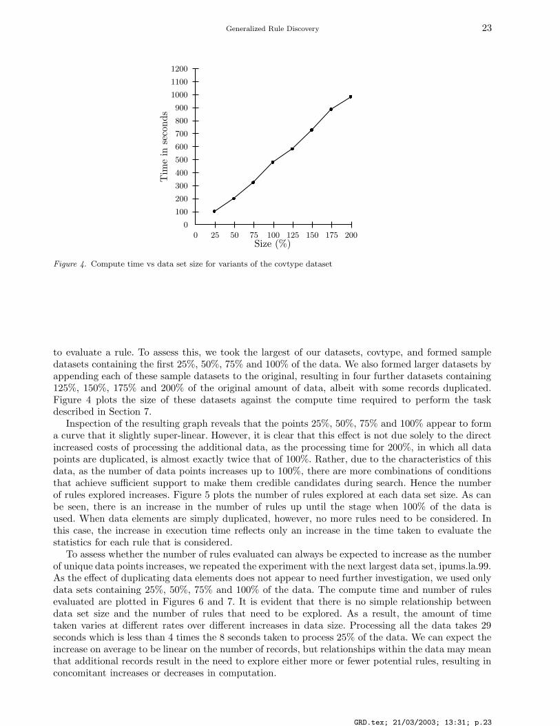
to evaluate a rule. To assess this, we took the largest of our datasets, covtype, and formed sampledatasets containing the first 25%, 50%, 75% and 100% of the data. We also formed larger datasets byappending each of these sample datasets to the original, resulting in four further datasets containing125%, 150%, 175% and 200% of the original amount of data, albeit with some records duplicated.Figure 4 plots the size of these datasets against the compute time required to perform the taskdescribed in Section 7.

Inspection of the resulting graph reveals that the points 25%, 50%, 75% and 100% appear to forma curve that it slightly super-linear. However, it is clear that this effect is not due solely to the directincreased costs of processing the additional data, as the processing time for 200%, in which all datapoints are duplicated, is almost exactly twice that of 100%. Rather, due to the characteristics of thisdata, as the number of data points increases up to 100%, there are more combinations of conditionsthat achieve sufficient support to make them credible candidates during search. Hence the numberof rules explored increases. Figure 5 plots the number of rules explored at each data set size. As canbe seen, there is an increase in the number of rules up until the stage when 100% of the data isused. When data elements are simply duplicated, however, no more rules need to be considered. Inthis case, the increase in execution time reflects only an increase in the time taken to evaluate thestatistics for each rule that is considered.

To assess whether the number of rules evaluated can always be expected to increase as the numberof unique data points increases, we repeated the experiment with the next largest data set, ipums.la.99.As the effect of duplicating data elements does not appear to need further investigation, we used onlydata sets containing 25%, 50%, 75% and 100% of the data. The compute time and number of rulesevaluated are plotted in Figures 6 and 7. It is evident that there is no simple relationship betweendata set size and the number of rules that need to be explored. As a result, the amount of timetaken varies at different rates over different increases in data size. Processing all the data takes 29seconds which is less than 4 times the 8 seconds taken to process 25% of the data. We can expect theincrease on average to be linear on the number of records, but relationships within the data may meanthat additional records result in the need to explore either more or fewer potential rules, resulting inconcomitant increases or decreases in computation.

GRD.tex; 21/03/2003; 13:31; p.23


0 25 50 75 100 125 150 175 200

0

10000

20000

30000

40000

50000

60000

70000

80000

90000

100000

110000

120000

130000

140000

150000

160000

�

�

�

�

� �

�

�

Size

Num

ber

ofru

les

eval

uat

ed

Figure 5. Number of rules evaluated vs data set size for variants of the covtype dataset

0 25 50 75 100

0

5

10

15

20

25

30

�

�

�

�

Size (%)

Tim

ein

seco

nds

Figure 6. Compute time vs data set size for variants of the ipums.la.99 dataset

9. Conclusions

Rule discovery techniques have evolved within two distinct paradigms, classification rule discoveryand association rule discovery. The focus of classification rule discovery on finding small sets of highlypredictive rules that jointly cover all available data is not well suited to contexts in which the primaryobjective is to gain insight into interactions within the data. While association rule discovery is directlyaimed at this objective, its support-confidence framework also limits its applicability. In particular,where minimum support is not a relevant criterion for selecting rules, the frequent itemset strategiesthat have been developed for association rule discovery risk failing to identify interesting rules.

We have presented a new framework for rule discovery which we call generalized rule discovery.Generalized rule discovery subsumes association rule discovery and the form of rule search generallyemployed to discover individual rules within classification rule discovery. We have presented a scalablealgorithm for generalized rule discovery. The computational complexity of the algorithm is linear with

GRD.tex; 21/03/2003; 13:31; p.24


0 25 50 75 100

0

10000

20000

30000

40000

50000

60000

70000

80000

90000

100000

110000 �

�

� �

Size

Num

ber

ofru

les

eval

uat

ed

Figure 7. Number of rules evaluated vs data set size for variants of the ipums.la.99 dataset

respect to data set size, although different sets of data imply different search spaces which may requiregreater or lesser computation to explore. We have demonstrated that GRD can efficiently solve aninteresting class of generalized rule discovery task, finding the 1000 rules with the highest leverage. Wehave further demonstrated that it is difficult to tackle this task using the frequent itemset frameworkpioneered within the association rule discovery paradigm.

An important benefit of the generalized rule discovery framework is the ability to impose andgain computational benefit from contraints on the maximum number of rules to discover. A commoncomplaint levelled against association rule discovery is that the user cannot control how many rules arereturned. The number of rules returned is controlled indirectly by the minimum support constraint.Small changes in this constraint can transform a problem for which very few rules are discoveredto one for which millions of rules are discovered. In the generalized rules discovery framework theuser can place an upper limit maxRules on the number of rules to discover. This constraint ensuresthat the user is only presented with the most interesting rules according to the specified measure ofinterestingness. It also speeds up the rule discovery task by allowing pruning of areas of the searchspace that cannot contain one of the maxRules most interesting rules.

This work demonstrates the efficiency of the GRD algorithm for one type of interesting rule dis-covery task. It falls to future research to identify further sets of interesting constraints for generalizedrule discovery and develop pruning rules that will facilitate their efficient solution.

Appendix

A. Proof of sufficiency and necessity of update strategy

The following theorems prove that the update strategy for currentSolution is sufficient and necessaryto ensure that on termination currentSolution = solution(〈A, C,D,M〉).

Theorem 12 (Sufficiency of currentSolution). Suppose GRDtask = 〈A, C,D,M〉. For any S ⊆{X → Y |X ⊆ A ∧ Y ⊆ C}, let currentSolution = solution(〈A, C,D,M ∧ X → Y ∈ S〉). For anys ∈ solution(〈A, C,D,M〉) ∩ S, s ∈ currentSolution holds.

This follows directly from (1).

Theorem 13 (Necessity of currentSolution). Suppose GRDtask = 〈A, C,D,M〉. For any S ⊆{X → Y |X ⊆ A ∧ Y ⊆ C}, let currentSolution = solution(〈A, C,D,M ∧ X → Y ∈ S〉). For anys ∈ currentSolution, s ∈ solution(〈A, C,D,M〉) ∩ S holds.

GRD.tex; 21/03/2003; 13:31; p.25


Proof. Assume there exists a rule s1 satisfies s1 ∈ currentSolution but s1 /∈ solution(〈A, C,D,M〉)∩S. So s1 /∈ solution(〈A, C,D,M〉) or s1 /∈ S holds. If s1 /∈ solution(〈A, C,D,M〉), then s1 /∈solution(〈A, C,D,M ∧ X → Y ∈ S〉), contradicting s1 ∈ currentSolution; if s1 /∈ S, obviouslys1 /∈ solution(〈A, C,D,M∧X→Y ∈ S〉), contradicting s1 ∈ currentSolution. Therefore s1 does notexist.

Due to the following theorem, it is not necessary to keep track of S. Rather, it is sufficient toupdate currentSolution as each rule is added to S.

Theorem 14 (Sufficiency of addition to currentSolution). Suppose GRDtask = 〈A, C,D,M〉.For any S ⊆ {X→Y |X ⊆ A∧Y ⊆ C} and rule r /∈ S, let currentSolution = solution(〈A, C,D,M∧X→Y ∈ S〉) and currentSolution′ = solution(〈A, C,D,M∧X→Y ∈ S∪{r}〉). The following holds.

solution(〈A, C,D,M∧ X→Y ∈ currentSolution ∪ {r}〉) ⊆ currentSolution′ (30)

Proof. Assume there exists a rule s1 that satisfies

s1 ∈ solution(〈A, C,D,M∧ X→Y ∈ currentSolution ∪ {r}〉) (31)

but s1 /∈ currentSolution′ which is

s1 /∈ solution(〈A, C,D,M∧ X→Y ∈ S ∪ {r}〉) (32)

According to the theorem of sufficiency of currentSolution, the following holds.

solution(〈A, C,D,M〉) ∩ (S ∪ {r}) ⊆ solution(〈A, C,D,M∧ X→Y ∈ S ∪ {r}〉) (33)

From (32) and (33), we obtain

s1 /∈ solution(〈A, C,D,M〉) ∩ (S ∪ {r}) (34)

From (31) we obtain s1 ∈ currentSolution∪ {r}. Let us first assume s1 ∈ currentSolution, which iss1 ∈ solution(〈A, C,D,M∧X→Y ∈ S〉). According to the theorem of necessity of currentSolution,s1 ∈ solution(〈A, C,D,M〉)∩S holds. Thus s1 ∈ S. So s1 ∈ S∪{r}. So s1 ∈ solution(〈A, C,D,M〉)∩(S ∪ {r}) holds, contradicting (34).

Now let us assume s1 ∈ {r}. This means s1 ∈ S ∪ {r}. From (31) and according to the theoremof necessity of currentSolution, s1 ∈ solution(〈A, C,D,M〉) ∩ (currentSolution ∪ {r}) holds. Thuss1 ∈ solution(〈A, C,D,M〉). From s1 ∈ S ∪ {r}, we obtain s1 ∈ solution(〈A, C,D,M〉) ∩ (S ∪ {r})holds, contradicting (34). Thus s1 does not exist. It follows that (30) holds.

Actually, the necessity of addition to currentSolution also holds, as shown in the following theorem.

Theorem 15 (Necessity of addition to currentSolution). Suppose GRDtask = 〈A, C,D,M〉.For any S ⊆ {X→Y |X ⊆ A∧Y ⊆ C} and rule r /∈ S, let currentSolution = solution(〈A, C,D,M∧X→Y ∈ S〉) and currentSolution′ = solution(〈A, C,D,M∧X→Y ∈ S∪{r}〉). The following holds.

currentSolution′ ⊆ solution(〈A, C,D,M∧ X→Y ∈ currentSolution ∪ {r}〉) (35)

Proof. For any s ∈ currentSolution′, which means s ∈ solution(〈A, C,D,M ∧ X → Y ∈ S ∪ {r}〉),according to the theorem of necessity of currentSolution, s ∈ solution(〈A, C,D,M〉) ∩ (S ∪ {r})holds. Thus

s ∈ solution(〈A, C,D,M〉) (36)

and s ∈ S ∪ {r} holds. Let us first assume s ∈ S. From (36), s ∈ solution(〈A, C,D,M〉) ∩ S.According to the theorem of sufficiency of currentSolution, s ∈ solution(〈A, C,D,M ∧ X → Y ∈S〉) = currentSolution. Thus s ∈ currentSolution ∪ {r}. Now let us assume s ∈ {r}. Obviouslys ∈ currentSolution ∪ {r} holds. Therefore we obtain

s ∈ currentSolution ∪ {r} (37)

From (36) and (37), s ∈ solution(〈A, C,D,M〉)∩(currentSolution∪{r}). According to the theorem ofsufficiency of currentSolution, we obtain s ∈ solution(〈A, C,D,M∧X→Y ∈ currentSolution∪{r}〉).Thus (35) holds.

GRD.tex; 21/03/2003; 13:31; p.26


Table IV. The generalized rule discovery algorithm without pruning

Algorithm: GRD′(CurrentLHS,AvailableLHS,AvailableRHS)

1: SoFar := ∅

2: for all P in AvailableLHS do

3: NewLHS := CurrentLHS ∪ {P}

4: NewAvailableLHS := SoFar

5: if P in AvailableRHS then

6: NewAvailableRHS := AvailableRHS - P

7: else

8: NewAvailableRHS := AvailableRHS

9: end if

10: for all Q in NewAvailableRHS do

11: if insolution(NewLHS → Q, 〈A, C,D,M∧ X→Y ∈ currentSolution ∪ {NewLHS→Q}〉) then

12: add NewLHS → Q to currentSolution

13: remove from currentSolution any rule W →Z : ¬insolution(W → Z,

〈A, C,D,M∧ X→Y ∈ currentSolution ∪ {NewLHS→Q}〉)

14: end if

15: end for

16: if NewAvailableLHS 6= ∅ and NewAvailableRHS 6= ∅ then

17: GRD′(NewLHS,NewAvailableLHS,NewAvailableRHS)

18: end if

19: SoFar := SoFar ∪ {P}

20: end for

B. Correctness of the GRD algorithm without pruning

By removing all the pruning in GRD, we get the GRD′ algorithm shown in Table IV. The correctnessof GRD′ is proven by its uniqueness and completeness. We first prove the completeness of GRD ′ inthe following theorem.

Theorem 16 (Completeness). Suppose GRDtask = 〈A, C,D,M〉. For any CurrentLHS,AvailableLHS ⊆ A and AvailableRHS ⊆ C satisfying AvailableLHS 6= ∅,AvailableRHS 6= ∅, CurrentLHS ∩ AvailableLHS = ∅ and CurrentLHS ∩AvailableRHS = ∅, let AvailableLHS = {P1, · · · , Pn} where n > 1 and P1, · · · , Pn ∈ A,let SEARCHED(CurrentLHS, {P1, · · · , Pm}, AvailableRHS) denote the set of rulesGRD′(CurrentLHS, AvailableLHS, AvailableRHS) has searched after the loop from P1 to Pm

at line 2 where 1 6 m 6 n, the following holds.

SEARCHED(CurrentLHS, {P1, · · · , Pm}, AvailableRHS) =

{CurrentLHS ∪ L→{Q}|L 6= ∅ ∧ L ⊆ {P1, · · · , Pm} ∧ Q ∈ AvailableRHS ∧ Q /∈ L}

Proof. The proof is by induction on m. For the basis, it is readily seen that the theorem is true whenm = 1, that is,

SEARCHED(CurrentLHS, {P1}, AvailableRHS) =

{CurrentLHS ∪ {P1}→{Q}|Q ∈ AvailableRHS ∧ Q 6= P1}

For the inductive hypothesis, assume that the theorem is true for 1 6 m 6 k. We willprove that the theorem is true for m = k + 1. When GRD′ loops at line 2 until Pk+1,SEARCHED(CurrentLHS, {P1, · · · , Pk, Pk+1}, AvailableRHS) is composed of two parts, one isSEARCHED(CurrentLHS, {P1, · · · , Pk}, AvailableRHS), and the other is the set of rules GRD′

searches from lines 3 to 19 for Pk+1. For Pk+1, from lines 3 to 15, GRD′ searches

{CurrentLHS ∪ {Pk+1}→{Q}|Q ∈ AvailableRHS ∧ Q 6= Pk+1}

GRD.tex; 21/03/2003; 13:31; p.27


and at line 17, GRD′(CurrentLHS ∪ {Pk+1}, {P1, · · · , Pk}, AvailableRHS) is called since at thispoint SoFar = {P1, · · · , Pk}. Applying the inductive hypothesis, we obtain:

SEARCHED(CurrentLHS, {P1, · · · , Pk, Pk+1}, AvailableRHS)

= SEARCHED(CurrentLHS, {P1, · · · , Pk}, AvailableRHS)

∪ {CurrentLHS ∪ {Pk+1}→{Q}|Q ∈ AvailableRHS ∧ Q 6= Pk+1}

∪ SEARCHED(CurrentLHS ∪ {Pk+1}, {P1, · · · , Pk}, AvailableRHS)


∪ {CurrentLHS ∪ {Pk+1}→{Q}|Q ∈ AvailableRHS ∧ Q 6= Pk+1}

∪ {CurrentLHS ∪ {Pk+1} ∪ L1→{Q}|L1 6= ∅ ∧ L1 ⊆ {P1, · · · , Pk}

∧ Q ∈ AvailableRHS ∧ Q /∈ L1 ∪ {Pk+1}}


∪ {CurrentLHS ∪ {Pk+1} ∪ L1→{Q}|L1 ⊆ {P1, · · · , Pk}

∧ Q ∈ AvailableRHS ∧ Q /∈ L1 ∪ {Pk+1}}

= {CurrentLHS ∪ L→{Q}|L 6= ∅ ∧ L ⊆ {P1, · · · , Pk} ∧ Q ∈ AvailableRHS ∧ Q /∈ L}

∪ {CurrentLHS ∪ {Pk+1} ∪ L1→{Q}|L1 ⊆ {P1, · · · , Pk} ∧ Q ∈ AvailableRHS

∧ Q /∈ L1 ∪ {Pk+1}}

= {CurrentLHS ∪ L→{Q}|L 6= ∅ ∧ L ⊆ {P1, · · · , Pk, Pk+1} ∧ Q ∈ AvailableRHS ∧ Q /∈ L}

proving the theorem.

For any GRDtask = 〈A, C,D,M〉, according to the theorem of sufficiency of addi-tion to currentSolution, the variable currentSolution at line 12 in GRD′ always recordssolution(〈A, C,D,M∧ X→Y ∈ S ∪ {r}〉) where S is the search space considered so far and r is thecurrent rule being considered. According to its completeness, when it finishes, GRD ′ has searched allthe rules, thus what the variable currentSolution records now is solution(〈A, C,D,M〉). This provesthe uniqueness of GRD′.

References

Agarwal, R. C., C. C. Aggarwal, and V. V. V. Prasad: 2000, ‘Depth First Generation of Long Patterns’. In: Proceedingsofthe Sixth ACM SIGKDD International Conference on Knowledge Discovery and Data Mining (KDD2000). Boston,MA, pp. 108–118, ACM.

Agrawal, R., T. Imielinski, and A. Swami: 1993, ‘Mining Associations between Sets of Items in Massive Databases’. In:Proceedings of the 1993 ACM-SIGMOD International Conference on Management of Data. Washington, DC, pp.207–216.

Agrawal, R., H. Mannila, R. Srikant, H. Toivonen, and A. I. Verkamo: 1996, ‘Fast Discovery of Association Rules’. In:U. M. Fayyad, G. Piatetsky-Shapiro, P. Smyth, and R. Uthurusamy (eds.): Advances in Knowledge Discovery andData Mining. Menlo Park, CA.: AAAI Press, pp. 307–328.

Agrawal, R. and R. Srikant: 1994, ‘Fast Algorithms for Mining Association Rules’. In: Proceedings of the 20thInternational Conference on Very Large Databases. Santiago, Chile, pp. 487–499.

Bay, S. D.: 2001, ‘The UCI KDD Archive’. [http://kdd.ics.uci.edu] Irvine, CA: University of California, Department ofInformation and Computer Science.

Bayardo, Roberto J., J.: 1998, ‘Efficiently Mining Long Patterns from Databases’. In: Proceedings of the 1998 ACM-SIGMOD International Conference on Management of Data. pp. 85–93.

Bayardo, Roberto J., J. and R. Agrawal: 1999, ‘Mining the Most Interesting Rules’. In: Proceedings of the Fifth ACMSIGKDD International Conference on Knowledge Discovery and Data Mining. pp. 145–154.

Bayardo, Roberto J., J., R. Agrawal, and D. Gunopulos: 2000, ‘Constraint-Based Rule Mining in Large, DenseDatabases’. Data Mining and Knowledge Discovery 4(2/3), 217–240.

Blake, C. and C. J. Merz: 2001, ‘UCI Repository of Machine Learning Databases’. [Machine-readable data repository].University of California, Department of Information and Computer Science, Irvine, CA.

Borgelt, C.: 2000, ‘Apriori’. (Computer Software) http://fuzzy.cs.Uni-Magdeburg.de/~borgelt/.

GRD.tex; 21/03/2003; 13:31; p.28


Buchanan, B. G. and E. A. Feigenbaum: 1978, ‘DENDRAL and Meta-DENDRAL: Their Applications Dimension’.Artificial Intelligence 11, 5–24.

Clark, P. and T. Niblett: 1989, ‘The CN2 Induction Algorithm’. Machine Learning 3, 261–284.Clearwater, S. H. and F. J. Provost: 1990, ‘RL4: A Tool for Knowledge-based Induction’. In: Proceedings of Second Intl.

IEEE Conf. on Tools for AI. Los Alamitos, CA, pp. 24–30, IEEE Computer Society Press.Cohen, E., M. Datar, S. Fujiwara, A. Gionis, R. Indyk, P. a nd Motwani, J. Ullman, and C. Yang: 2000, ‘Finding

Interesting Associations without Support Pruning’. In: Proceedings International Conference on Data Engineering.Cohen, W. W.: 1995, ‘Fast Effective Rule Induction’. In: Proceedings of the Twelfth International Conference on Machine

Learning. Morgan Kaufmann.Han, J., J. Pei, and Y. Yin: 2000, ‘Mining Frequent Patterns without Candidate Generation’. In: Proc. 2000 ACM-

SIGMOD Int. Conf. on Management of Data (SIGMOD’00). Dallas, TX, pp. 1–12.Kohavi, R., C. Brodley, B. Frasca, L. Mason, and Z. Zheng: 2000, ‘KDD-Cup 2000 organizers’ report: Peeling the onion’.

SIGKDD Explorations 2(2), 86–98.Liu, B., W. Hsu, and Y. Ma: 1998, ‘Integrating Classification and Association Rule Mining’. In: Proceedings Knowledge

Discovery and Data Mining (KDD-98). pp. 80–86.Liu, B., W. Hsu, and Y. Ma: 1999, ‘Mining Association Rules with Multiple Minimum Supports’. In: Proceedings of the

ACM SIGKDD International Conference on Knowledge Discovery and Data Mining (KDD-99). San Diego, CA, pp.337–341.

Michalski, R. S.: 1977, ‘Synthesis of Optimal and Quasi-optimal Variable-valued Logic Formulas’. In: Proceedings of the1975 International Symposium on Multiple Valued Logic. Bloomington, Indiana, pp. 76–87, Reidel.

Morishita, S. and A. Nakaya: 2000, ‘Parallel Branch-and-Bound Graph Search for Correlated Association Rules’. In:Proceedings of the ACM SIGKDD Workshop on Large-Scale Parallel KDD Systems, Vol. LNAI 1759. Berlin: Springer,pp. 127–144.

Pasquier, N., Y. Bastide, R. Taouil, and L. Lakhal: 1999, ‘Discovering frequent closed itemsets for association rules’. In:Proceedings of the Seventh International Conference on Database Theory (ICDT’99). Jerusalem, Israel, pp. 398–416.

Pei, J., J. Han, and R. Mao: 2000, ‘CLOSET: An Efficient Algorithm for Mining Frequent Closed Itemsets’. In: Proc.2000 ACM-SIGMOD Int. Workshop on Data Mining and Knowledge Discovery (DMKD’00). Dallas, TX, pp. 21–30.

Piatetsky-Shapiro, G.: 1991, ‘Discovery, Analysis, and Presentation of Strong Rules’. In: G. Piatetsky-Shapiro and J.Frawley (eds.): Knowledge Discovery in Databases. AAAI/MIT Press, pp. 229–248.

Provost, F., J. Aronis, and B. Buchanan: 1999, ‘Rule-Space Search for Knowledge-Based Discovery’. CIIO WorkingPaper IS 99-012, Stern School of Business, New York University, , NY, NY 10012.

Rymon, R.: 1992, ‘Search through Systematic Set Enumeration’. In: Proceedings KR-92. Cambridge, MA, pp. 268–275.Savasere, A., E. Omiecinski, and S. Navathe: 1995, ‘An Efficient Algorithm for Mining Association Rules in Large

Databases’. In: Proceedings of the 21st International Conference on Very Large Data Bases. pp. 432–444, MorganKaufmann.

Segal, R. and O. Etzioni: 1994, ‘Learning Decision Lists Using Homogeneous Rules’. In: AAAI-94. Seattle, WA, AAAIpress.

Todorovski, L., P. Flach, and N. Lavrac: 2000, ‘Predictive Performance of Weighted Relative Accuracy’. In: D. A.Zighed, J. Komorowski, and J. Zytkow (eds.): Proceedings of the Fourth European Conference on Principles of DataMining and Knowledge Discovery (PKDD2000). pp. 255–264, Springer-Verlag.

Toivonen, H.: 1996, ‘Sampling Large Databases for Association Rules’. In: Proceedings of the 22nd InternationalConference on Very Large Data Bases. pp. 134–145, Morgan Kaufmann.

Webb, G. I.: 1995, ‘OPUS: An Efficient Admissible Algorithm for Unordered Search’. Journal of Artificial IntelligenceResearch 3, 431–465.

Webb, G. I.: 2000, ‘Efficient search for association rules’. In: The Sixth ACM SIGKDD International Conference onKnowledge Discovery and Data Mining. Boston, MA, pp. 99–107, The Association for Computing Machinery.

Zaki, M. J.: 2000, ‘Generating Non-Redundant Association Rules’. In: Proceedings of the Sixth ACM SIGKDDInternational Conference on Knowledge Discovery and Data Mining (KDD2000). Boston, MA, pp. 34–43, ACM.

Zheng, Z., R. Kohavi, and L. Mason: 2001, ‘Real World Performance of Association Rule Algorithms’. In: KDD-2001:Proceedings of the Seventh International Conference on Knowledge Discovery and Data Mining. San Francisco, pp.401–406, ACM.

GRD.tex; 21/03/2003; 13:31; p.29

GRD.tex; 21/03/2003; 13:31; p.30

Beyond Association Rules: Generalized Rule Discovery Rules/Beyond... · Beyond Association Rules:...

Documents

Transcript of Beyond Association Rules: Generalized Rule Discovery Rules/Beyond... · Beyond Association Rules:...