Bexhill Hastings Link Road Best and Final Funding Bid ... · Best and Final Funding Bid Assignment...

Bexhill Hastings Link RoadBest and Final Funding BidAssignment Model Validation Report

Bexhill Hastings LinkRoad

Best and FinalFunding Bid

Assignment ModelValidation Report

East Sussex County CouncilCounty HallSt Anne's CrescentLewesEast Sussex


Bexhill Hastings LinkRoad

Best and FinalFunding Bid

Assignment ModelValidation Report

Issue and Revision RecordRev Date Originator Checker Approver Description

A March 2009 N Gordon/P Shears I Johnston I Johnston For Issue

B July 2011N Gordon

I Johnston I Johnston Issued for comments

C August2011

N GordonI Johnston I Johnston For Issue

Bexhill Hastings Link RoadBest and Final Funding BidAssignment Model Report

i

List of Contents Page

Chapters and Appendices

1 Introduction...............................................................................................................1

2 SATURN Model Description .....................................................................................2

2.1 Introduction...............................................................................................................2

2.2 Network Description..................................................................................................2

2.3 Zoning System..........................................................................................................4

3 SATURN Matrices ..................................................................................................11

3.1 Roadside Interview Surveys ...................................................................................11

3.2 Observed Matrix Building........................................................................................11

3.3 Prior Matrix .............................................................................................................13

3.4 Matrix Estimation ....................................................................................................14

4 SATURN Model Assignment...................................................................................22

4.1 Assignment.............................................................................................................22

4.2 Network calibration and model convergence ..........................................................22

5 SATURN Model Validation......................................................................................24

5.1 Validation Criteria ...................................................................................................24

5.2 Calibration Results .................................................................................................24

5.3 Flow Validation .......................................................................................................25

5.4 Journey Time Validation .........................................................................................32

5.5 Additional Journey Time Validation.........................................................................39

5.6 Internal Trip Distribution..........................................................................................41

6 Public Transport Model...........................................................................................46

6.1 Model Network........................................................................................................46

6.2 Matrices..................................................................................................................48

6.3 Bus Fares ...............................................................................................................53

6.4 Rail validation .........................................................................................................54

6.5 Bus validation .........................................................................................................55

7 Present Year Validation ..........................................................................................57

7.2 2011 Reference Highway Matrix Totals ..................................................................59

7.3 2011 Reference public transport matrices...............................................................60

7.4 2011 Present Year Highway Validation...................................................................62


2

7.5 A271 Flow Adjustment............................................................................................65

7.6 Journey Time Validation .........................................................................................73

8 Conclusion..............................................................................................................79

List of Figures

Figure 2-1: Glyne Gap September 2004 ATC daily profile ......................................................2Figure 2-2: Model Network Area.............................................................................................5Figure 2-3: Speed Flow Curves ..............................................................................................6Figure 2-4: Local Zoning System - Bexhill ..............................................................................7Figure 2-5: Local Zoning System – Hastings ..........................................................................8Figure 2-6: External Zoning System .......................................................................................9Figure 2-7: Zoning System UK .............................................................................................10Figure 3-1: Roadside Interview Locations.............................................................................18Figure 3-2: Sectors in the Study Area...................................................................................19Figure 3-3: AM Trip Length Distribution ................................................................................20Figure 3-4: IP Trip Length Distribution..................................................................................20Figure 3-5: PM Trip Length Distribution ................................................................................21Figure 5-1: AM Flow Validation Screenlines .........................................................................35Figure 5-2: IP Flow Validation Screenlines ...........................................................................36Figure 5-3: PM Flow Validation Screenlines .........................................................................37Figure 5-4: Journey Time Survey Routes .............................................................................38Figure 5-5: Baldslow Journey Time Routes ..........................................................................40Figure 5-6: Bexhill Ward Subsets .........................................................................................44Figure 5-7: Hastings Ward Subsets......................................................................................45Figure 6-1: Local Bus Routes ...............................................................................................47Figure 7-1: AM Peak Modelled Flows (total vehs (hgv%)) ....................................................69Figure 7-2: Interpeak Modelled Flows (total vehs (hgv%)) ....................................................70Figure 7-3: PM Peak Modelled Flows (total vehs (hgv%)) ....................................................71Figure 7-1: Journey Time Survey Routes .............................................................................74

List of Tables

Table 2.1: Speed Flow Curve Data.........................................................................................3Table 3.1: RSI Sample Rates ...............................................................................................11Table 3.2: Roadside Interview Survey Factors .....................................................................12Table 3.3: RSI Matrix User Class Split..................................................................................13Table 3.4: Matrix Data by Sector ..........................................................................................14Table 3.5: Pre Matrix Estimation Trips..................................................................................15Table 3.6: Post Matrix Estimation Trips ................................................................................16Table 4.1: Generalised Cost Parameters..............................................................................22Table 4.2: Convergence Parameters....................................................................................23Table 4.3: Achieved Convergence........................................................................................23Table 5.1: Assignment Validation - Acceptability Guidelines.................................................24Table 5.2: Flow Calibration Results (Counts used for Matrix Estimation)..............................25Table 5.3: AM Peak RSI Flow Calibration.............................................................................26Table 5.4: Inter Peak RSI Flow Calibration...........................................................................27Table 5.5: PM Peak RSI Flow Calibration.............................................................................28


3

Table 5.6: AM Peak Screenline Flow Validation ...................................................................29Table 5.7: Interpeak Screenline Flow Validation...................................................................30Table 5.8: PM Peak Screenline Flow Validation ...................................................................31Table 5.9: AM Peak Journey Time Validation .......................................................................33Table 5.10: Interpeak Journey Time Validation.....................................................................33Table 5.11: PM Peak Journey Time Validation .....................................................................34Table 5.12: Baldslow AM Peak Journey Time Comparison ..................................................40Table 5.13: Baldslow Interpeak Journey Time Comparison..................................................41Table 5.14: Baldslow PM Peak Journey Time Comparison ..................................................41Table 5.15: Bexhill Census Distribution ................................................................................42Table 5.16: Bexhill Modelled Distribution..............................................................................42Table 5.17: Hastings Census Distribution.............................................................................43Table 5.18: Hastings Modelled Distribution ..........................................................................43Table 6.1: Weekday and weekend assumed splits by ticket group .......................................49Table 6.2: Outward time of travel assumptions by ticket group.............................................50Table 6.3: Return time of travel assumptions by ticket group................................................50Table 6.4: Journey purpose by ticket group assumptions .....................................................51Table 6.5: Journey purpose by time of travel assumptions ...................................................51Table 6.6: Rail Trip Car Availability Split ...............................................................................52Table 6.7: Split of Trips by Time Period and Journey Purpose .............................................53Table 6.8: Bus Trip Car Availability Split ...............................................................................53Table 6.9: AM (0800-0900) Peak Rail Passenger Validation ................................................54Table 6.10: Interpeak (1000-1600 average) Rail Passenger Validation ................................55Table 6.11: PM Peak (1600-1800 average) Rail Passenger Validation.................................55Table 6.12: Bus Passengers Validation Results ...................................................................56Table 7.1: Main Business Developments in Bexhill and Hastings (2004-2011).....................57Table 7.2: Housing Completions 2004-2011.........................................................................58Table 7.3: Central Growth Rate for LGV and HGV ...............................................................59Table 7.4: AM Peak Matrix Totals.........................................................................................59Table 7.5: Interpeak Matrix Totals ........................................................................................60Table 7.6: PM Peak Matrix Totals.........................................................................................60Table 7.7: AM Peak Public Transport Matrix Totals ..............................................................61Table 7.8: Interpeak Public Transport Matrix Totals..............................................................61Table 7.9: PM Peak Public Matrix Totals ..............................................................................61Table 7-10: DIADEM parameters .........................................................................................62Table 7.11: AM Peak Flow Validation...................................................................................63Table 7.12: Inter Peak Flow Validation .................................................................................64Table 7.13: PM Peak Flow Validation...................................................................................65Table 7.14: AM Peak Flow Validation post matrix estimation................................................66Table 7.15: Inter Peak Flow Validation post matrix estimation..............................................67Table 7.16: PM Peak Flow Validation post matrix estimation................................................68Table 7.17: AM Peak Journey Time Validation .....................................................................76Table 7.18: Interpeak Journey Time Validation.....................................................................77Table 7.19: PM Peak Journey Time Validation .....................................................................78

Bexhill Hastings Link RoadBest and Final Funding BidAssignment Model Report

1

1 Introduction

1.1.1 This report describes the Hastings Bexhill traffic model created in 2004and validated to 2004 traffic flows. The model was updated in line with variabledemand modelling guidance issued in September 2005.

1.1.2 To ensure the different variable demand responses can be assessedaccurately, the model has five separate user classes of cars commuting, cars onemployers business, other cars, light good vehicles and heavy goods vehicles.The model has been validated to an average September 2004 weekday for threetime periods, am, interpeak and pm peak period.

1.1.3 The report also describes the present year validation undertaken usingMay 2011 survey data


2

2 SATURN Model Description

2.1 Introduction

2.1.1 The model was built using the SATURN suite of programs. Analysis ofthe Highways Agency Automatic Traffic Counter Data at Glyne Gap has beenused to determine the modelled periods. The am peak is represented by the hourbetween 0800 and 0900. The interpeak model is for an average hour between1000 and 1600and the PM peak model assesses an average hour between 1600and 1800 as the ATC revealed little difference in flow levels of these two hours.Figure 2.1 shows the daily profile at the Glyne Gap ATC site.

Figure 2-1: Glyne Gap September 2004 ATC daily profile

0

200

400

600

800

1000

1200

1400

1600

1800

2000

2200

2400

2600

1 2 3 4 5 6 7 8 9 10 11 12 13 14 15 16 17 18 19 20 21 22 23 24

Hour Ending

Flo

w(v

ehs)

Eastbound

Westbound

Total

2.1.2 The model has been built to represent an average weekday inSeptember 2004 as this was the only neutral month in 2004 for which a completemonths’ worth of ATC data was available.

2.2 Network Description

2.2.1 The geographical extend of the model network, and the links andjunctions included, is shown in Figure 2.2. The network is comprised ofsimulation areas and buffer areas. The simulation area extends to Pevensey Bayin the West, Battle in the North and Icklesham in the East. The main corridors inthe area are the A259 between Pevensey Bay and Icklesham, the A269 betweenBoreham Street and Bexhill, the A2102 and the A21 between Sedlescombe and


3

Hastings, the A28 from Bede to Baldslow and the B2093 between Baldslow andOre.

2.2.2 The buffer network extends to Hailsham in the west, Robertsbridge inthe north and Rye in the east. All link lengths, number of lanes and widths usedin the model were checked against 1:2500 scale AutoCAD drawings to ensurethat the roads had been correctly coded.

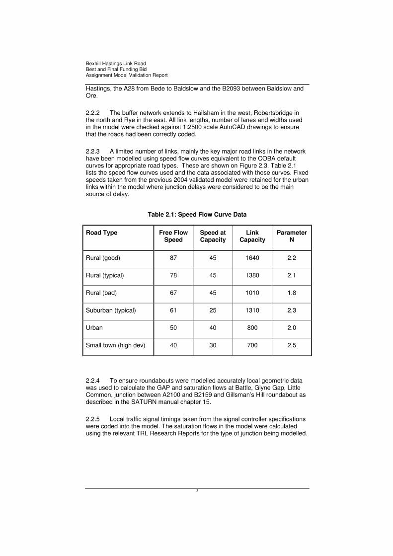
2.2.3 A limited number of links, mainly the key major road links in the networkhave been modelled using speed flow curves equivalent to the COBA defaultcurves for appropriate road types. These are shown on Figure 2.3. Table 2.1lists the speed flow curves used and the data associated with those curves. Fixedspeeds taken from the previous 2004 validated model were retained for the urbanlinks within the model where junction delays were considered to be the mainsource of delay.

Table 2.1: Speed Flow Curve Data

Road Type Free FlowSpeed

Speed atCapacity

LinkCapacity

ParameterN

Rural (good) 87 45 1640 2.2

Rural (typical) 78 45 1380 2.1

Rural (bad) 67 45 1010 1.8

Suburban (typical) 61 25 1310 2.3

Urban 50 40 800 2.0

Small town (high dev) 40 30 700 2.5

2.2.4 To ensure roundabouts were modelled accurately local geometric datawas used to calculate the GAP and saturation flows at Battle, Glyne Gap, LittleCommon, junction between A2100 and B2159 and Gillsman’s Hill roundabout asdescribed in the SATURN manual chapter 15.

2.2.5 Local traffic signal timings taken from the signal controller specificationswere coded into the model. The saturation flows in the model were calculatedusing the relevant TRL Research Reports for the type of junction being modelled.


4

2.3 Zoning System

2.3.1 The zoning system includes smaller zones covering the simulation areaand external zones to ensure full trip lengths were coded into the model. Theexternal zones were based on combinations of census output areas, districts andcounty boundaries. Figures 2.4 and 2.5 show the local Bexhill and Hastingszoning system, whilst Figures 2.6 and 2.7 detail the external zones.


5

Figure 2-2: Model Network Area


10

Figure 2-7: Zoning System UK


11

3 SATURN Matrices

3.1 Roadside Interview Surveys

3.1.1 Roadside Interview Survey (RSI) Data was available at four locations asshown on Figure 3.1. The surveys on the A259 at Glyne Gap and the B2095 andA271 west of Battle were undertaken in May 2002 as part of LATS. ESCC carriedout RSI’s at Glyne Gap in the opposite direction to the London Area TransportSurvey (LATS) in April 2004 and on Crowhurst Road in June 2005.

3.1.2 To ensure the model includes as much observed data as possible, all ofthe above surveys have been included in the matrix building process.

3.2 Observed Matrix Building

3.2.1 The above LATS and ESCC roadside interview (RSI) data were used toderive the observed matrices. These were the key sites for establishing the east-west movement through the study area.

3.2.2 Table 3.1 below shows a comparison of the sample rate achieved ateach site and the rate required for the sample to be accurate to 5% within a 95%confidence interval. The Glyne Gap westbound survey is just outside the requiredsample rate but all other survey locations achieved the required sample rate.

Table 3.1: RSI Sample Rates

Survey SampleRate

RequiredSample Rate

A271 21% 19%

B2096 33% 32%

A259 Glyne Gapwestbound

9% 10%

A259 Glyne Gapeastbound

18% 11%

Crowhurst Road 84% 54%


12

3.2.3 The interview sample records were multiplied up to the total recordedsurvey day flow on the link by half hour or hourly factors. These factors are givenin Appendix B of the Traffic Survey Report. The following hours of interviewrecords were used for each modelled hour matrix building:

• AM Peak: 08:00 - 09:00

• Interpeak: 10:00 – 16:00

• PM Peak: 16:00 - 1800

3.2.4 The observed RSI data were then factored to September 2004 torepresent the base year. The conversion factors used for each site for each timeperiod were shown in Table 3.2. These factors were calculated by comparing theflow from the Glyne Gap ATC site for the day of the RSI survey with an averageSeptember 2004 flow. Matrices were created for 5 different user classes as CarCommuting, Car Business, Car Other, LGV and HGV.

Table 3.2: Roadside Interview Survey Factors

Conversion Factor

Sites Survey Date AM IP PM

LATS at A259 at Glyne Gap,B2095 and A271 west ofBattle

May 2002 1.21 1.26 1.13

RSI’s at Glyne Gap April 2004 1.15 1.10 1.09

RSI’s at Crowhurst Road June 2005 1.04 1.01 0.99

3.2.5 For the Crowhurst Road, B2095 and A271 sites, the pm peak RSI matrixwas transposed and added to the am peak RSI direction to give total am peakflows, and the am peak RSI matrix was transposed and added to the pm peakRSI direction to give total pm peak flows. For the Interpeak period, the RSIdirection matrix was added to a transpose of itself to give total Interpeak flows.

3.2.6 The matrices for the different sites were then added together by userclass and time period. To produce the final observed matrices the different userclass matrices were stacked separately for each time period.

3.2.7 The interpeak and pm peak hour matrices were then divided by six andtwo respectively to obtain average hourly matrices for the modelled time periods.The final RSI matrices had the following split of user classes by time period.


13

Table 3.3: RSI Matrix User Class Split

AM Peak Interpeak PM Peak

Cars – commuting 51% 12% 40%

Cars – employersbusiness

7% 12% 7%

Cars – other 27% 57% 37%

LGVs 12% 14% 13%

HGVs 3% 5% 3%

All 100% 100% 100%

3.3 Prior Matrix

3.3.1 As mentioned above, the RSI sites provided observed east-westmovements through the study area. They would not have picked up internalBexhill or internal Hastings trips. To provide an initial estimate of the internalBexhill and Hastings trips, these elements were extracted from the final validatedmatrices of the previous (2004) model.

3.3.2 The previous model took its internal Hastings and Bexhill trips from the1997 Hastings Bexhill Transport Study model. Tempro growth rates were appliedthen matrix estimation was used to match observed data.

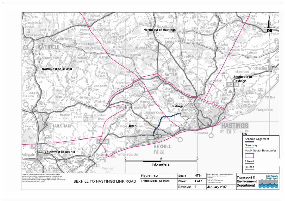
3.3.3 Table 3.4 shows the provenance of the data used to build the pre matrixestimation matrices on a sector basis. The sectors are Hastings, Bexhill, SW ofBexhill, NW of Bexhill, SE of Hastings and NE of Hastings. Figure 3.2 shows thelocation of the sectors used.


14

Table 3.4: Matrix Data by Sector

1 2 3 4 5 6

Hastings Bexhill Southwestof Bexhill

Northwestof Bexhill

SoutheastofHastings

NortheastofHastings

1 Hastings 2004model

RSIdata RSI data RSI data

2004model

2004model

2 Bexhill RSI data2004model

2004model

2004model

RSI data RSI data

3 Southwestof Bexhill RSI data

2004model

2004model

2004model

RSI data RSI data

4 Northwestof Bexhill RSI data

2004model

2004model

2004model RSI data RSI data

5 SoutheastofHastings

2004model

RSIdata

RSI data RSI data2004model

2004model

6 NortheastofHastings

2004model

RSIdata

RSI data RSI data2004model

2004model

3.4 Matrix Estimation

3.4.1 A selection of the count data from both manual classified counts andautomatic counts were used for matrix estimation. The zone to zone flowsthrough the RSI survey sites were frozen during this process. Tables 3.6 and 3.7show the pre and post matrix estimation trip totals by sector. Trip totals for allsectors and time periods reduced slightly during matrix and sector to sectorchanges are minor.


15

Table 3.5: Pre Matrix Estimation Trips

AM Peak

Sectors 1 2 3 4 5 6 Total

1 13,808 1,189 394 375 426 1,772 17,963

2 1,250 7,097 464 1,016 13 201 10,041

3 455 542 0 15 26 113 1,150

4 547 647 17 13 4 183 1,412

5 646 85 43 29 114 76 994

6 1,766 272 143 142 51 76 2,451

Total 18,473 9,832 1,062 1,591 634 2,420 34,011

Interpeak


1 11,678 880 303 272 367 1,210 14,710

2 832 6,412 309 605 36 177 8,371

3 289 406 5 6 19 93 817

4 272 567 4 18 13 95 970

5 402 47 8 7 99 61 624

6 1,171 217 93 83 55 63 1,682

Total 14,643 8,529 722 992 589 1,698 27,174


16

PM Peak


1 13,839 1,142 535 538 492 1,446 17,992

2 1,115 6,547 848 834 39 260 9,643

3 450 789 0 17 38 184 1,477

4 474 934 15 13 39 182 1,658

5 454 41 14 3 107 43 663

6 1,652 250 117 187 71 39 2,318

Total 17,984 9,702 1,530 1,593 786 2,155 33,751

Table 3.6: Post Matrix Estimation Trips

AM Peak


1 14,030 1,050 422 302 355 1,353 17,512

2 1,242 6,862 534 635 11 187 9,471

3 424 373 0 15 18 135 965

4 506 324 17 11 2 198 1,058

5 436 78 42 28 79 78 741

6 1,244 220 169 154 55 91 1,934

Total 17,882 8,907 1,184 1,146 521 2,042 31,682


17

Interpeak


1 12,242 857 340 290 307 972 15,006

2 795 6,463 302 381 36 212 8,189

3 253 300 5 6 14 73 651

4 278 313 4 18 13 76 703

5 299 46 7 7 71 46 477

6 948 186 91 82 47 93 1,448

Total 14,815 8,165 749 785 489 1,472 26,475

PM Peak


1 14,621 1,155 489 410 401 1,175 18,252

2 1,029 6,947 560 513 40 222 9,312

3 383 578 0 17 32 169 1,180

4 465 608 15 11 44 173 1,315

5 323 35 14 3 92 32 499

6 1,240 265 76 92 85 106 1,865

Total 18,063 9,587 1,155 1,046 694 1,877 32,422

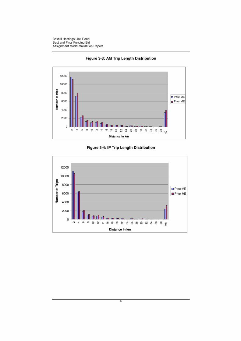
3.4.2 Figures 3.3 to 3.5 show the trip length distribution for all three timeperiods from before and after the matrix estimation process. It is again apparentthat the distribution changes are small and the pattern of changes is similar in alltime periods.


20

Figure 3-3: AM Trip Length Distribution

0

2000

4000

6000

8000

10000

12000

2 4 6 8 10 12 14 16 18 20 22 24 26 28 30 32 34 36 38

40+

Distance in km

Nu

mb

ero

ftr

ips

Post ME

Prior ME

Figure 3-4: IP Trip Length Distribution

0

2000

4000

6000

8000

10000

12000

2 4 6 8 10 12 14 16 18 20 22 24 26 28 30 32 34 36 38

40+

Distance in km

Nu

mb

ero

fT

rip

s

Post ME

Prior ME


21

Figure 3-5: PM Trip Length Distribution

0

2000

4000

6000

8000

10000

120002 4 6 8 10 12 14 16 18 20 22 24 26 28 30 32 34 36 38 40+

Distance in km

Nu

mb

ero

fTri

ps

Post ME

Prior ME


22

4 SATURN Model Assignment

4.1 Assignment

4.1.1 The separate trip matrices produced for each time period were stackedbefore being assigned to the model network. The heavy vehicle matrices weremultiplied by a factor of 2 to convert them to pcu equivalents.

4.1.2 A pre-peak hour has been modelled for the am and pm peak periods toensure the appropriate level of queues and delays were modelled. The matricesfor the pre-peak hour were a proportion, 90 % of the peak hour matrices, basedon analysis of September 2004 ATC daily profile at Glyne Gap.

4.1.3 The generalised cost parameters for each vehicle type were calculatedusing values of time and fuel operating costs from WebTAG and a weightedaverage produced. This gave the parameters for time, PPM (pence per minute)and distance, PPK (pence per kilometre) as shown in Table 4.1. More detail onthe calculation is provided in Appendix A, and the full spreadsheet calculation issupplied electronically.

Table 4.1: Generalised Cost Parameters

PPM (penceper minute)

PPK (pence perkilometre)

Car Commuting 1 0.45

Car Business 1 0.25

Car Other 1 0.32

LGV 1 0.75

HGV 1 2.54

4.1.4 Using these parameters, the matrices were then assigned usingWardrop Equilibrium assignment method.

4.2 Network calibration and model convergence

4.2.1 The network was calibrated by independent checking of the link lengthsand junction layouts against OS mapping and site visit notes. Evidence of the linklength checks undertaken is provided in Appendix B. Routes between zoneswere also checked to ensure sensible route choice was occurring.


23

4.2.2 Route choice was identified in the model and checked for logical routing,while junction coding was compared against layouts observed during site visits.Evidence of some sample calibration checks have been added to Appendix B.

4.2.3 The convergence parameters used ensured that each of the am,interpeak and pm peak models met all of the DMRB Volume 12 (Section 2 Part 1Appendix H) criteria given below:

Table 4.2: Convergence Parameters

Convergence Measure Acceptable Value

Duality gap � Less than 1%

AND one of the following

Percentage of links with flow change <5%

Four consecutive iterations greater than95%

Relative Absolute Average Difference(RAAD) in flows

Less than 1%

AAD in flows Less than 1 veh/hr

4.2.4 To ensure the model was well converged, the validation criteria for flowchanges between loops was tightened to a difference of 2% for 97% of links inthe network. A ‘tighter’ convergence of the SATURN highway network is alsoessential for variable demand modelling using DIADEM and to get robusteconomic results with TUBA. Table 4.3 below shows the final convergenceparameters for each of the modelled parameters:

Table 4.3: Achieved Convergence

Timeperiod

DualityGap (%)

No of loopswith flow

change <2%

RAAD (%) AAD(pcu/hr)

AM 0.051 4 0.29 0.59

IP 0.017 4 0.18 0.31

PM 0.034 4 0.24 0.49

Bexhill Hastings Link Road Best and Final Funding Bid ... · Best and Final Funding Bid Assignment...

Documents

Transcript of Bexhill Hastings Link Road Best and Final Funding Bid ... · Best and Final Funding Bid Assignment...