Between-Firm Redistribution of Profitin Competitive Industries:

Why Labor Market Policies May Not Work∗

Galina Vereshchagina†

Abstract

Empirical studies document differences in firms’ response to theintroduction of various labor market policies. In particular, large andmature firms tend to participate more actively in the targeted employ-ment subsidy programs (under which firms receive subsidies for hiringdisadvantaged workers). This paper offers an explanation for this phe-nomenon and argues that it might have important consequences forpolicy making.

Namely, such behavior of firms may indicate that large and maturefirms benefit from the introduction of the new subsidy program, whilesmall and young firms incur indirect cost. In this case, the policyimplicitly redistributes profit from young to mature firms and maydiscourage startups if the entry into the industry is competitive. Theresulting decrease in the number of operating firms is likely to have asignificant impact on the policy’s outcomes. These effects are gettingmore pronounced as heterogeneity between young and mature firmsincreases.

∗This research was supported by a grant from CERGE-EI Foundation under a programof the Global Development Network. All opinions expressed are those of the author andhave not been endorsed by CERGE-EI, WIIW, or the GDN.

†Contact address: CERGE-EI, Politickych veznu 7, 111 21 Prague 1, Czech Republic,gala@cerge-ei.cz.

1

1 Introduction

In economies with substantial firm heterogeneity, some firms may incur losseswhile others may benefit as a result of a new labor market policy introducedby the government. In other words, the policy may redistribute profit amongdifferent groups of firms. This paper argues that such redistribution mayhave important implications for policymaking if (i) entry into the industryis competitive and (ii) there are substantial differences in size or productiv-ity between young and mature firms. In particular, if mature firms are theones who, for some reason, benefit from the introduction of a labor marketpolicy, the expected lifetime profit of entrants may decrease, thereby discour-aging start-ups and reducing the number of operating firms. Naturally, theresulting decline of the size of the production sector might have importantimplications for policy analysis.

For example, a government may introduce an employment subsidy pro-gram aimed at increasing economy’ total employment level. While designingthis program, a policymaker may believe that either the policy would haveno impact on the number of firms operating in the economy or that it wouldaffect entrants as much as mature firms. Relying on these assumptions, thepolicymaker would expect that the new subsidy program would reduce econ-omy’s unemployment level. However, this paper presents a theory and anumerical example illustrating that the opposite may happen after the pol-icy is implemented, due to the adverse effect on total employment caused bya massive exit of firms.

This study focuses on the effects of are the employment subsidies paid tothe firms hiring workers with particular characteristics (e.g., having relativelylow skills, being long term unemployed). Even though such policy is primarilytargeted to a special group of workers, it also implicitly favors those firmswho either create relatively more jobs for the workers from the targeted groupor appear to be more responsive to a decrease in these workers’ labor cost.

Several versions of such targeted employment subsidy programs have beenused by policymakers in different countries during the last decade.1 Availabil-ity of the data about the participants in these subsidy programs stimulateda large number of empirical studies evaluating their outcomes. Some of theseworks focus on the labor market perspectives of the targeted group of work-

1The examples of such policies include Targeted Job Tax Credit in the U.S., New Dealin Britain, various wage subsidies in Canada and Sweden, etc.

2

ers, others study displacement effects and potential deadweight losses, severalmore focus on the subsidies’ effects on aggregate employment in a particularsector.2 At the same time, there is no unanimous agreement regarding thesuccess of these subsidy programs because empirical evidence is quite con-troversial and depends on the program’s setup, its scale, size of the targetedgroup and many other factors. In contribution to the existing literature, thispaper suggests that the heterogeneity between young and mature firms mightserve as a potential explanatory variable in the empirical analysis evaluatingthe targeted employment subsidy programs. The theory developed in thisstudy predicts that, in the competitive industries, the bigger are the differ-ences between young and mature firms, the more likely it is that the subsidyprogram will not be successful.

Despite much attention that the existing theoretical literature has paidto understanding the impacts of various labor market policies and identify-ing the important mechanisms responsible for the policies’ outcomes, therehas not been, to my knowledge, any study focusing primarily on the role ofbetween-firm redistribution driven by the introduction of a new policy. Apossible reason for such gap in the literature is that in many cases the as-sumptions used in theoretical models do not allow to account fully for therelationship between this redistribution effect and the number of firms oper-ating in the economy. For example, some studies explicitly assume that thenumber of firms in the industry is fixed at an exogenously given level andcannot change in response to an introduction of a new policy.3 Another classof models allows to pin down the number of firms endogenously, but relieson the assumption that the entrants are no different from the mature firms,thereby neglecting the potential effect that redistribution of profit betweenfirms with different characteristics may have on the the number of firms inthe economy.4

A different approach is taken in the work by Hopenhayn and Rogerson(1993), in which the impacts of firing taxes are analyzed in the context ofindustry dynamics framework with heterogeneous firms and endogenous en-

2See, for example, Bishop and Montgomery (1986), Hollenbeck and Willke (1991),Katz (1996), Bell, Blundell and Van Reen (1999), Blundell and Meghir (2001), Calmfors,Forslund and Hemstrom (2001), Martin and Grebb (2001), Sianesi (2001) and many others.

3See, for example Alvarez and Veracierto (2000), Richardson (1997), etc.4In Mortensen and Pissarides (1998) the number of vacancies is determined endoge-

nously, but it is assumed that entrants draw a productivity shock from the same distribu-tion as older firms do.

3

try and exit flows. Their paper draws attention to the welfare implicationsof the firing taxation program as well as its impacts on the productivity ofentering and surviving firms. At the same time, it neither describes the re-distributionary effects of the policy nor poinst out their potential importancefor policy analysis. That is why, in the current paper I modify Hopenhaynand Rogerson’s (1993) framework and use it to study the response of theeconomy to the introduction of targeted employment subsidy program. Thegoal of this exercise is to identify the role of between-firm redistribution inexplaining some of the policy’s outcomes.

The theoretical framework developed in this paper is based on a simplemodel of industry equilibrium with heterogeneity on both sides of the labormarket. Firms differ in their size and age, which are positively related toeach other. As in Hopenhayn (1992), entry into the industry is competi-tive, so in the equilibrium the value of entrants, measured as their expecteddiscounted life-time flow of profit, is equal to the cost of starting a new enter-prize. Workers have different skills, and low-skilled workers ought to receiveadditional training before starting their job. For this reason, in the equilib-rium low-skilled workers receive lower wage and have higher unemploymentrate than high-skilled workers do.

Firms incur a cost for training unskilled employees. Empirical evidencesuggests that larger firms tend to provide more training per one employedworker5 as well as to participate more actively in the subsidy programs6.These implications endogenously arise in the model if the training cost func-tion is convex in the fraction of firms’ unskilled employees. Intuitively, iffirms’ production technology is concave, the convexity of the training cost iseasily derived from the assumption that skilled workers have to spend someof their working time training their unskilled colleagues rather than produc-ing. In reality, firms report that much of the training they provide is indeeddone in this way.7

Another implication of the training cost’s convexity explains why the gov-ernment might consider employment subsidies for hiring unskilled workers asa good policy instrument aimed at increasing total employment. It turns outthat in response to a decrease in the wage of unskilled workers every operat-

5For instance, see the data from the 1995 Survey of Employer-Provided Training col-lected by the Bureau of Labor Statistics (Sept95).

6For evidence see Bishop and Montgomery (1986).7In Sept95 survey firms report that over 70 percent of training is usually delivered

through informal instructions rather then officially organized classes.

4

ing firm not only decides to hire more unskilled employees, but also createsmore jobs for skilled workers. Intuitively, if a firm hires more employees re-quiring additional training, it must also hire more workers, who are able toprovide training services, otherwise training all new unskilled hires becomestoo expensive. Such complementarity in the workers’ types gives a hope thatsubsidizing unskilled workers would stimulate demand for both types of laborand, consequently, would raise aggregate employment.

The above argument would be correct if the number of firms in the econ-omy were not affected by the subsidy program. However, if the number ofoperating firms is determined endogenously, the subsidy could induce somefirms to exit and the total unemployment could rise. For example, a cal-ibrated numerical exercise shows that if 30% of unskilled workers’ wage issubsidized by the government, aggregate unemployment rate falls from 6%to 3.4% in the economy with the constant number of firms. On the otherhand, it turns out the same subsidy increases unemployment from 6% to7.6% if the number of firms is determined endogenously.

In general, exit of firms from the economy could occur for two reasons:either because the subsidy program redistributes profit from entrants to ma-ture firms or because the subsidy expenditures are financed by a distortionarytax. That is why, in order to illustrate the importance of the former redis-tributionary effect, the second part of the numerical exercise compares thecalibrated benchmark economy, in which entrants are 68% smaller than in-cumbent firms, with the economy where the entrants are only 41% smallerthan the incumbents. In the absence of subsidies, the equilibrium allocationsin the two economies are identical. However, it turns out that if the samesubsidy program is implemented in both economies, fewer firms exit from theeconomy with relatively large entrants, and, therefore, the resulting equilib-rium unemployment rate is higher in the economy with more heterogeneitybetween young and mature firms. In particular, the 30% subsidy, which in-duces unemployment rate to rise to 7.6% in the benchmark economy, reducesunemployment to 4.7% in the modified economy with larger entrants.

The remaining of the paper is organized as follows. Section 2 describesfirms’ decision in a partial equilibrium framework, explains in details why andhow the redistribution effect may occur and derives the aggregate economy’sdemand for both types of labor. Section 3 describes how the equilibriumallocation in the economy is determined and argues that accounting for en-dogeneity of the number of firms is likely to have an important effect. Section4 describes the calibration technique and summarizes the results of numerical

5

policy experiments. Section 5 outlines the main findings of the paper andcomments on some of the assumption made in the theoretical model.

2 Firms’ Hiring Decision

This Section characterizes employment decision of firms in a partial equilib-rium framework. It shows that, under the assumption of a convex trainingcost, large firms, as compared to the small ones, hire more unskilled labor,incur higher training expenditures and, correspondingly, benefit more fromthe introduction of targeted employment subsidies. This is done in two steps.First, I describe the hiring policies of firms in a static setup and analyze theeffects of employment subsidies on one-period firms’ profits. Then I showthat static results can be extended to a dynamic setting. The last part ofthe Section describes the aggregate firm dynamics, derives the economy’s de-mand for both types of labor and discusses why the introduction of targetedemployment subsidies may affect the total number of firms in the economy.

2.1 The effect of targeted employment subsidies onfirms’ current profit

Consider an economy in which there are two types of workers, skilled andunskilled. Only skilled employees can be productively working in a firm.That is why, if a firm hires unskilled workers it must provide them with acertain amount of training. Training is costly. Firms’ training cost riseswith the number nl of unskilled hires and falls with the amount nh of skilledemployees. Without loss of generality, it is assumed that the training cost canbe represented as a function of the fraction of unskilled to skilled employees,nl/nh. I also assume that the training cost is convex in nl/nh:

c

(nl

nh

)=

(nl

Anh

)1+γ

, (1)

where A > 0 and γ > 0 for all nh > 0 and nl > 0. As it is shown later, theassumption of convexity allows to obtain a positive relationship between thefirm size and the amount of training provided by the firm, which is observedin the data.8

8In a more general case, these properties of the cost function c(nh, nl) could be derivedendogenously under the assumption that skilled employees have to spend some of their

6

Given this cost function and the wages wh and wl paid to skilled andunskilled workers respectively, every firm decides how many employees ofeach type it wants to hire. Hiring decision is made in the very beginningof the period, then training is provided for unskilled workers, and after thatproduction takes place. Since unskilled workers become identical to skilledemployees after the former receive necessary training, firms’ output can beexpressed as a function of total employment l = nh + nl. The productiontechnology is given by sf(l), where f(·) is a concave increasing productionfunction having the property of decreasing returns to scale and satisfyingInada conditions, s ∈ [0, s] is a firm productivity level. Productivity israndom and follows Markov process with the conditional distribution givenby Q(s′|s).

For simplicity, I assume that firms face no fixed production cost, thusinstantaneous profit of a firm having productivity shock s and hiring nh andnl workers of each type is given by

π(s, nh, nl; wh, wl) = sf(nh + nl)− whnh − wlnl − c(nl/nh).

Note that, due to the absence of a fixed cost, a firm hiring no workers pro-duces no output and pays no cost, so its profit is equal to zero, π(s, 0, 0) = 0.

The optimal hiring policies n∗h(s; wh, wl) and n∗l (s; wh, wl) are derived ina simple profit maximization problem:

π∗(s; wh, wl) = maxnh,nl

{π(s, nh, nl; wh, wl)} (2)

The following Lemma describes the properties of the firms’ hiring decision.

Lemma 1 If f(·) satisfies Inada conditions, wh > wl and the training costfunction c(·) is given by (1) then

(i) for every s > 0 there exist a unique set of hiring policies n∗h(s; wh, wl) >0 and n∗l (s; wh, wl) > 0, which solve (2);

(ii) total employment l∗(s; wh, wl) = n∗h(s; wh, wl) + n∗l (s; wh, wl) and thefraction of unskilled employees n∗l (s; wh, wl)/l

∗(s; wh, wl) are increasingin firms’ productivity level s.

working time training their unskilled colleagues. Assuming that λ units of time are requiredto train one worker, one can easily show that endogenous cost of hiring arising in thisenvironment satisfies the following conditions for some λ < 1 and all λ > λ: c1(nh, nl) < 0,c2(nh, nl) > 0, c11(nh, nl) > 0, c12(nh, nl) < 0, and c22(nh, nl) > 0. It is straightforwardto verify that similar properties hold for the cost function determined by (1).

7

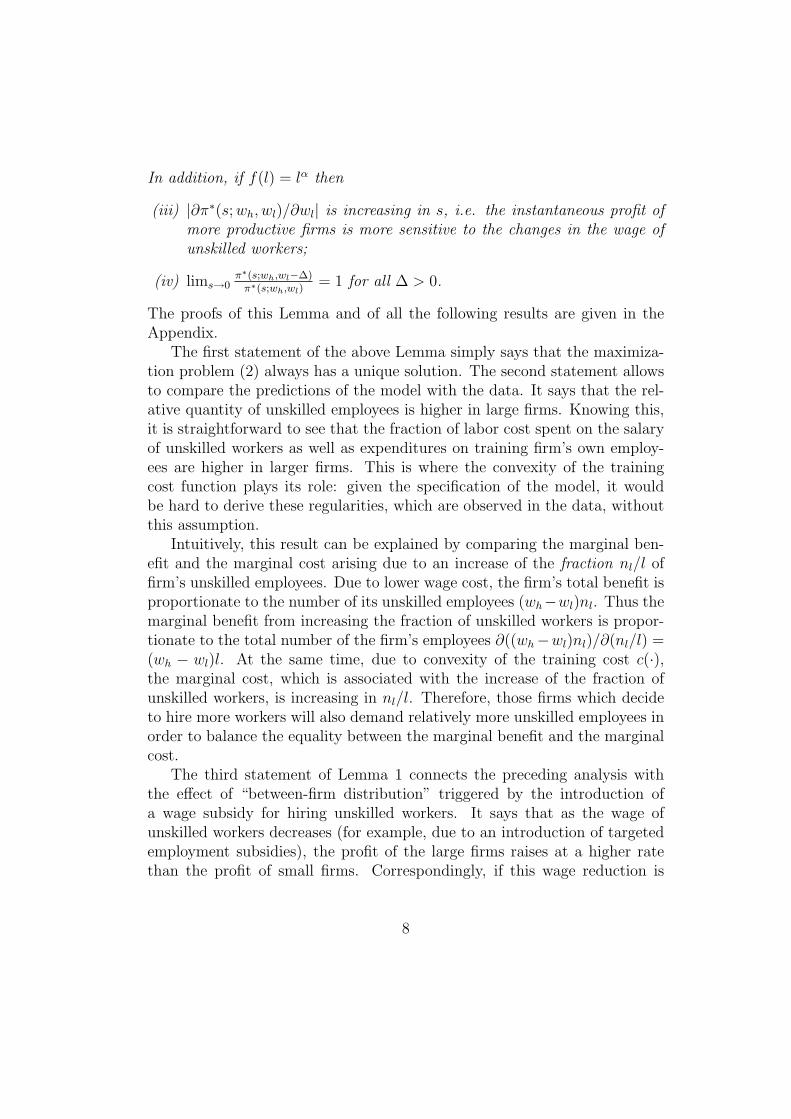
In addition, if f(l) = lα then

(iii) |∂π∗(s; wh, wl)/∂wl| is increasing in s, i.e. the instantaneous profit ofmore productive firms is more sensitive to the changes in the wage ofunskilled workers;

(iv) lims→0π∗(s;wh,wl−∆)

π∗(s;wh,wl)= 1 for all ∆ > 0.

The proofs of this Lemma and of all the following results are given in theAppendix.

The first statement of the above Lemma simply says that the maximiza-tion problem (2) always has a unique solution. The second statement allowsto compare the predictions of the model with the data. It says that the rel-ative quantity of unskilled employees is higher in large firms. Knowing this,it is straightforward to see that the fraction of labor cost spent on the salaryof unskilled workers as well as expenditures on training firm’s own employ-ees are higher in larger firms. This is where the convexity of the trainingcost function plays its role: given the specification of the model, it wouldbe hard to derive these regularities, which are observed in the data, withoutthis assumption.

Intuitively, this result can be explained by comparing the marginal ben-efit and the marginal cost arising due to an increase of the fraction nl/l offirm’s unskilled employees. Due to lower wage cost, the firm’s total benefit isproportionate to the number of its unskilled employees (wh−wl)nl. Thus themarginal benefit from increasing the fraction of unskilled workers is propor-tionate to the total number of the firm’s employees ∂((wh−wl)nl)/∂(nl/l) =(wh − wl)l. At the same time, due to convexity of the training cost c(·),the marginal cost, which is associated with the increase of the fraction ofunskilled workers, is increasing in nl/l. Therefore, those firms which decideto hire more workers will also demand relatively more unskilled employees inorder to balance the equality between the marginal benefit and the marginalcost.

The third statement of Lemma 1 connects the preceding analysis withthe effect of “between-firm distribution” triggered by the introduction ofa wage subsidy for hiring unskilled workers. It says that as the wage ofunskilled workers decreases (for example, due to an introduction of targetedemployment subsidies), the profit of the large firms raises at a higher ratethan the profit of small firms. Correspondingly, if this wage reduction is

8

financed by a proportionate profit tax9, the after-tax profit decreases for thesmall firms and rises for the large ones after the subsidy is introduced.

For better exposition, Figure 1 (in the end of the paper) illustrates therelative change in the profit as a function of firms’ productivity that occursif wage of unskilled workers falls by 10 per cent. The left panel plots thechange in before-tax profit, π∗(s; wh, (1 − θ)wl)/π

∗(s; wh, wl). Note that,according to the last statement of Lemma 1, the profit of a very smallfirm is very little affected by the wage reduction. This happens becausesmall firms hire very few of unskilled workers. The right panel of Figure 1plots the after-tax change in the profit. For every positive tax rate τ > 0,lims→0((1 − τ)π∗(s; wh, (1 − θ)wl)/π

∗(s; wh, wl)) < 1, so all firms with rela-tively low productivity levels (s < s∗) experience a decrease in instantaneousprofit, and those with s > s∗ benefit from the introduction of the subsidy.Obviously, in this example the tax rate is chosen arbitrarily (τ = 0.05). Ina general equilibrium framework it is determined by a government budgetconstraint, which is later defined in Section 4.

2.2 The effect of targeted employment subsidies onfirms’ life-time value

This Section characterizes the stay/exit decision of the firms that have al-ready entered into the industry and argues that introduction of a subsidyfor unskilled employees, financed by a profit tax, decreases the value of smallfirms and increases the value of the large ones. Entry decision and its relationto aggregate dynamics are described in the following section.

Assume that firms decide whether to stay or exit before the realizationof their current productivity shock. If the outside opportunity is normalizedto zero, the value of the firm that has decided to stay in the industry in thecurrent period is given by

V (s; wh, wl) = π∗(s; wh, wl) +1

1 + rmax

{0,

∫V (s′; wh, wl)dQ(s′|s)

}, (3)

9It is easy to see that if the subsidy is financed by a payroll tax, or by the tax on thewage income of skilled employees, the same redistribution effect occurs. In the latter case,it even becomes stronger because an implicit increase in the relative labor cost of skilledemployees works in the same direction as a reduction of the wage of unskilled workers,thereby reinforcing the redistribution effect.

9

where r denotes a risk-free interest rate. Before characterizing the propertiesof V (s; wh, wl) I make the following assumptions about the properties of theprocess of firms’ productivity shocks:

ASSUMPTION 1 (Continuity and monotonicity) Q(s′|s) is continu-ous in both s and s′; Q(·|s) is strictly decreasing in s.

Continuity implies that if V (s′; wh, wl) is a continuous function of s′ then∫V (s′; wh, wl)dQ(s′|s) is also continuous in s. From monotonicity it follows

that the integral in the right hand side of equation (3) preserves the mono-tonicity of V (s′; wh, wl) with respect to s′.

ASSUMPTION 2 (Absorbing state) Q(0|0) = 1, i.e. s = 0 is an ab-sorbing state.

In the modelled environment this assumption is necessary to generatepositive flows of entry and exit. Due to the absence of a fixed production cost,the current profit of firms is nonnegative at any level of productivity shock.Correspondingly, the value of the firm with zero productivity level wouldbe positive if assumption 2 were not imposed (because even not operationalfirms would have a positive probability of becoming productive again in thefuture), and no exit would ever occur. The absence of a fixed productioncost is obviously a simplifying assumption but it allows to abstract from thepolicy’s impact on the average productivity in the industry, thus allowing tofocus on the between-firms distributional effect.

In addition, Assumption 2 guarantees that the after-tax present value ofexpected life-time profit decreases for the firms with sufficiently low produc-tivity levels after the targeted employment subsidy is introduced. If s = 0were not an absorbing state it could happen that the value of small firmswould increase after the introduction of the subsidy, given that the probabil-ity of getting high productivity in the future is large enough. On the otherhand, if low productivity shocks are sufficiently persistent (as it is reportedin the data), the results of Lemma 2 will still be valid even if Assumption 2does not imply. In other words, neither of the two implications of Assump-tion 2 is crucial for the validity of the main argument of the paper, but theyboth allow conveying the idea in a more illustrative way.

Lemma 2 If all assumptions of Lemma 1 hold and the process of firms’productivity shocks satisfies Assumptions 1 and 2 then dynamic programmingproblem (3) has a unique solution V (s; wh, wl), such that:

10

(i) V (s; wh, wl) is increasing and continuous in s, V (s; wh, wl) > 0 if andonly if s > 0;

(ii) |∂V (s; wh, wl)/∂wl| is increasing in s;

(iii) lims→0V (s;wh,(1−ε)wl)

V (s;wh,wl)= 1 for all ε ∈ (0, 1);

(iv) for every ε ∈ (0, 1) and τ > 0 there exist such s that Vτ (s; wh, (1 −ε)wl) < V (s; wh, wl) for all s < s, where

Vτ (s; wh, (1− ε)wl) =(1− τ)π∗(s; wh, (1− ε)wl)+

+1

1 + rmax

{0,

∫Vτ (s

′; wh, (1− ε)wl)dQ(s′|s)}

.

(4)

Lemma 2 establishes that the properties of the instantaneous profit π∗(s; wh, wl)are mapped into similar properties of the firms’ life-time value V (s; wh, wl),and only the firms with sufficiently high productivity levels (s > s) maybenefit from the presence of the targeted employment subsidies (conditionalon the tax rate τ and wages wh and wl being fixed).

In order to proceed with the definitions of the equilibrium it is now nec-essary to describe how the distribution of firms’ productivity levels evolvesover time and how it relates to the distribution of entrants’ productivityshocks and the number of entering firms. This mechanism is characterizedin the following Section and is similar to the formalization of firm dynamicsin Hopenhayn (1993).

2.3 Aggregate Firm Dynamics

In the beginning of each period, before the individual productivity shocks aredrawn, an unlimited number of potential firms faces an option of entering intothe industry. If a firm decides to enter it draws a productivity shock from thedistribution characterized by c.d.f. G(s), s ∈ [0, s]. Its future productivityshocks follow Markov process Q(s′|s) described above. Opening up a firmrequires fixed cost η, which should be paid before the initial productivityshock is drawn.

If the markets are perfectly competitive, entry into the industry occurs aslong as the present value of expected life-time profit for the entrants exceeds

11

entry cost η. No firms are willing to enter if the following condition holds:∫

V (s; wh, wl)dG(s) = η. (5)

The above free entry condition determines the equilibrium number of firmsentering into the industry every period. It is balanced through the mechanismof wage determination on the labor market. For example, if too many firmsenter, the aggregate demand for labor input is very large. If the number ofpotential workers is limited (e.g., the population size is restricted), high labordemand drives wages up and pushes firms’ expected value below the entrycost. This makes entry unprofitable and discourages potential start ups. Onthe contrary, if very few firms enter, the wages are low and firms’ profits arehigh. In this case, the number of entering firms increases until the equalityis reached in the free entry condition (5).

Equation (5) plays the crucial role in analyzing the effects of labor marketpolicies. In particular, the larger is the decrease in the left hand side ofthe free entry condition generated by the introduction of the employmentsubsidy, the more firms would have to exit from the industry, and, as aconsequence, aggregate employment may fall. This is likely to happen ifthe distribution of entrants’ productivity shocks is concentrated over therelatively small values of s, because, as it has been shown in the previousSection, the after-tax value of sufficiently small firms decreases when thesubsidy program is implemented.

To describe formally the link between the aggregate labor demand and theflow of entrants, one has to characterize the low of motion of the distributionof firms’ productivity shocks. Assume that by the end of the period t theaggregate distribution of firms’ productivity levels is described by the densityfunction µt(S) (S is form the Borel set of [0, s]) and λt+1 firms decide to enterinto the industry in the beginning of the period t + 1, then the distributionof firms’ productivity shocks µt+1 by the end of the period t + 1 is given by

µt+1([0, s′]) =

∫

s∈(0,s)

Q(s′|s)dµt(s) + λt+1G(s′)

The first term in the above expression describes how the distribution of ex-isting firms changes from period t to period t+1 and accounts for those firmswho receive productivity shock s = 0 in period t and exit from the indus-try. The second term adds to it the distribution of newcomers’ productivityshocks.

12

ASSUMPTION 3 For every s ∈ [0, s] there exist N ≥ 1 such thatQN(0|s) > 0.

This assumption suggests that every firm exits with positive probabilitywithin a finite number of periods. As a consequence of this assumption,it can be shown that every firm’s expected life-time is finite. Precisely thiscondition is driving the existence of stationary distribution of firms’ produc-tivity shocks in the long run.

Lemma 3 If Q(s′|s) satisfies Assumptions 1-3, G(0) < 1 and λt = λ for allt ≥ 0 then

(i) there exists a unique distribution µλ such that T nµ0 ⇒ µλ for every µ0:

µλ([0, s′)) =

∫

s∈(0,s)

Q(s′|s)dµλ(s) + λG(s′); (6)

(ii) if λ1 = kλ then µλ1 = kµλ.

(Proof of Lemma 3 follows the line of argument in Hopenhayn (1993).)In other words, the presence of absorbing state guarantees the existence of

unique invariant distribution µλ with a relatively limited number of assump-tions. Intuitively, the evolution of µt can be decomposed into two processes.On one hand, as time goes on, more of those firms, who were present in theindustry at time 0, exit. After sufficiently many periods very few of them re-main active, therefore the limiting distribution µλ (if it exists) is not affectedby the initial distribution µ0. On the other hand, λ firms open up everyperiod and at least some of them receive positive productivity shocks (sinceG(0) < 1). This prevents the industry from dying out. The fact that everyfirm’s expected life time is finite guarantees that the distribution generatedby the inflow of new firms every period does not explode and converges to afinite distribution µλ, as it is stated in (i) of Lemma 3.

Therefore, if the number of entrants λ and the distribution of their pro-ductivity shocks G(·) are known, the aggregate labor demands in the sta-tionary allocation are given by

NDh (wh, wl, λ) =

∫ s

0

nh(s; wh, wl)dµλ(s), (7)

NDl (wh, wl, λ) =

∫ s

0

nl(s; wh, wl)dµλ(s). (8)

13

Before switching to a formal definition of an equilibrium allocations, itis useful to formulate the following result describing the properties of theaggregate labor demand:

Lemma 4 Assume that f(l) = lα, α ∈ (0, 1), c(·) is given by (1) and Q(s′|s)satisfies Assumptions 1-3. Then for every λ > 0

(i)∂ND

l (wh,wl,λ)

∂wl< 0 and

∂NDh (wh,wl,λ)

∂wh< 0.

(ii) If, in addition, wl

wh< 1− 1−α

1+γthen

∂NDh (wh,wl,λ)

∂wl< 0.

The above Lemma characterizes how aggregate demands for labor respondto the changes in the wage rates. Part (i) of Lemma 4 states an obvious result:if a wage for any type of labor falls, firms respond by hiring more workersof this type. The second result of Lemma 4 is less obvious and is drivenby the convexity of the training cost as a function of a fraction of unskilledemployees. In particular, part (ii) claims that a decrease in the wage ofunskilled workers not only stimulates the demand for unskilled labor but alsodrives up the demand for skilled employees, thus creating a complementaritybetween both types of workers.

Intuitively, in response to a decrease in wl the firm would primarily in-crease the number of its unskilled workers. If, at the same time, the firm doesnot adjust the number of its skilled employees, the fraction nl/nh increasestoo fast. Since the training cost is convex, this could imply that the firm’sexpenditures on training grow faster than its benefits resulting from a fall inwl. Thus, in order to slow down the growth of the marginal training cost,the firm must also increase the number of its unskilled employees.

Obviously, the above argument will apply only if the degree of convex-ity of the training cost function is large enough, which is stipulated by thecondition wl

wh< 1 − 1−α

1+γthat appears in (ii) of Lemma 4. Note that the

firm’s productivity s does not enter this inequality, implying that the twotypes of labor are substitutes in all incumbent firms, independent of theirsize. Clearly, this condition could be relaxed if certain properties are knownabout the distribution of firms’ productivity shocks µλ. In particular, forevery individual firm the result of (ii) would hold if its current fraction ofunskilled workers nl/(nl + nh) is small enough (it is easy to verify that thestatement is always true if nl/(nl + nh) → 0).

However, even in its general form the condition wl

wh< 1 − 1−α

1+γis not too

restrictive, as it is illustrated on Figure 2 in the Appendix. In particular, the

14

top panels of Figure 2 draw the subsets of (α, γ), which satisfy this conditionfor different wl/wh. For example, if α = 0.64 (which corresponds to a laborshare of output observed in the data) and wl/wh = 0.66 (which is consistentwith the wage distribution observed in the data10), all positive values of γsatisfy this sufficient condition.

Recalling that the assumption of convexity of training cost can be derivedfrom the assumption of on-job training provided by the skilled employees totheir less skilled colleagues, the second result of Lemma 4 becomes very intu-itive: if a firm increases a number of employees requiring additional training,it must also hire more workers, who are able to provide this training, other-wise it incurs too large losses.

Such complementarity property is obviously an extreme case and is un-likely to find a strong support in the data. However, it turns out to be veryhelpful in conveying the main argument of the paper: I show that even inthe presence of such complementarity, redistributional effect can revert thepredictions of policy analysis. Lemma 4 implies that a reduction in the wagefor unskilled workers would stimulate demand for both types of employees,thus suggesting that the introduction of employment subsidy could poten-tially have a positive impact on total employment if the number of entrantsλ remains unchanged. However, this prediction may fail if λ is determinedendogenously because an increase in labor demand for skilled workers canbe outweighed by an endogenous decrease in the number of operating firmsarising due to profit redistribution from young to mature firms. This channelis studied more carefully in the following Section.

3 Equilibrium Allocation and Policy Analysis

This Section defines an equilibrium allocation and explains why accountingfor general equilibrium effects, arising due to endogeneity of the numberof firms in the economy, might have important implications for evaluatingemployment subsidy programs. The analysis in the first part of the Sectiondoes not specify how labor supply is generated because the results formulatedbelow hold for any increasing labor supply function. However, a particularshape of labor supply has to be chosen if one wants to relate the results to thedata and analyze numerically the effects of targeted employment subsidies.

10The relation between wl and wh is described in details in Section 4 while summarizingthe calibration methodology.

15

That is why the last part of this Section presents one possible example ofendogenizing labor supply curves and explaining how unemployment arises.

3.1 Stationary equilibrium allocation

Assume that the labor supply curves of both types of labor are given by theupward sloping functions NS

h (wh) and NSl (wl).

11

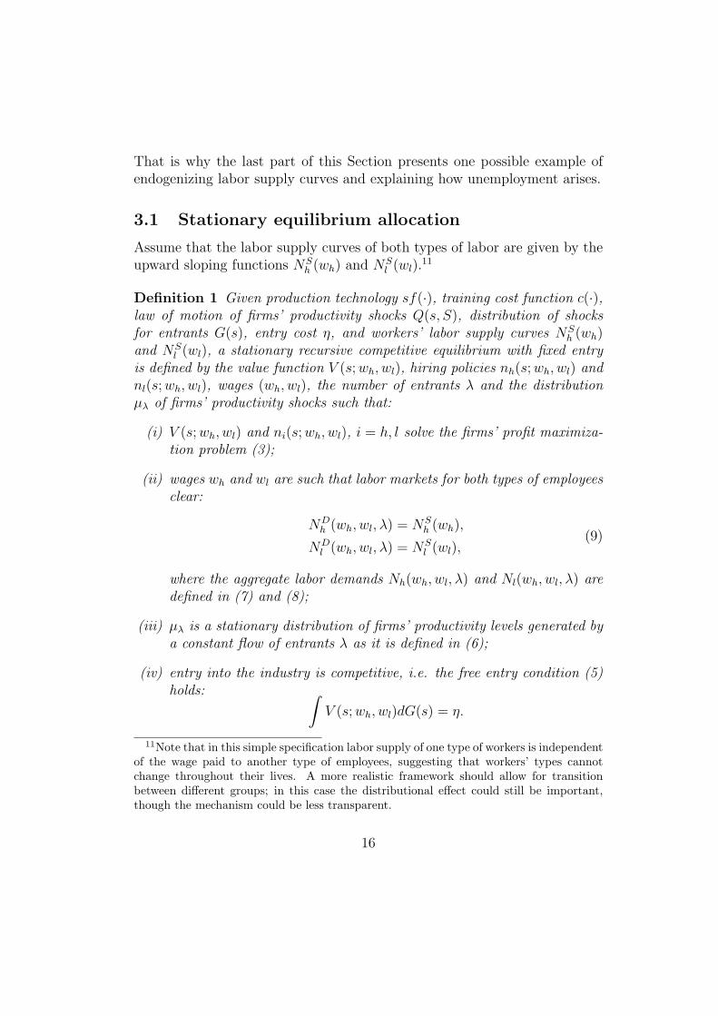
Definition 1 Given production technology sf(·), training cost function c(·),law of motion of firms’ productivity shocks Q(s, S), distribution of shocksfor entrants G(s), entry cost η, and workers’ labor supply curves NS

h (wh)and NS

l (wl), a stationary recursive competitive equilibrium with fixed entryis defined by the value function V (s; wh, wl), hiring policies nh(s; wh, wl) andnl(s; wh, wl), wages (wh, wl), the number of entrants λ and the distributionµλ of firms’ productivity shocks such that:

(i) V (s; wh, wl) and ni(s; wh, wl), i = h, l solve the firms’ profit maximiza-tion problem (3);

(ii) wages wh and wl are such that labor markets for both types of employeesclear:

NDh (wh, wl, λ) = NS

h (wh),

NDl (wh, wl, λ) = NS

l (wl),(9)

where the aggregate labor demands Nh(wh, wl, λ) and Nl(wh, wl, λ) aredefined in (7) and (8);

(iii) µλ is a stationary distribution of firms’ productivity levels generated bya constant flow of entrants λ as it is defined in (6);

(iv) entry into the industry is competitive, i.e. the free entry condition (5)holds: ∫

V (s; wh, wl)dG(s) = η.

11Note that in this simple specification labor supply of one type of workers is independentof the wage paid to another type of employees, suggesting that workers’ types cannotchange throughout their lives. A more realistic framework should allow for transitionbetween different groups; in this case the distributional effect could still be important,though the mechanism could be less transparent.

16

In the remainder of the paper this equilibrium allocation is referred to asa free entry equilibrium because it stipulates that the free entry condition issatisfied with equality. Altogether, conditions (9) and (5) constitute a systemof three equations with three unknown aggregate variables - wages wh andwl, and the number of entrants λ.

As an alternative to a free entry equilibrium, one could also consider aneconomy where the total number of firms is fixed endogenously, i.e. λ is aparameter rather than exogenous variable. In such economy the free entrycondition (5) would not necessarily hold, while the conditions (i)-(iii) wouldstill have to be satisfied in an equilibrium allocation. For convenience, let uslabel such equilibrium allocation, characterized by an exogenous parameterλ, as a fixed entry equilibrium with λ entrants.12

3.2 The effects of targeted employment subsidies

Consider the following policy experiment. Assume that the government sub-sidizes firms for hiring unskilled workers by compensating a fraction θ ofthese workers’ wage wl. Suppose that the government finances these subsidyexpenditures by levying a profit tax at a flat rate τ . This means that firms’cost of hiring an unskilled worker drops to (1 − θ)wl, and, correspondingly,firms’ value Vτ (s; wh, (1 − θ)wl) is now given by the maximization problem(4). Note also that profit tax financing does not affect firms’ hiring policies,because their labor decision is derived from instantaneous profit maximiza-tion problem.13

In an equilibrium allocation, the government should determine tax and

12In a general case, it is not possible to claim either existence or uniqueness of any of thedefined above equilibria. Multiple equilibria can occur due to the fact that the condition

NDh (wh, wl, λ)

NDl (wh, wl, λ)

=Nh(wh)Nl(wl)

,

which should always hold in the equilibrium due to (9), may generate a non-monotonerelationship between wl and wh for any given λ. That is why in the numerical examplein the last Section of the paper I choose such set of the parameters that the benchmarkfree entry equilibrium is unique, and then study the deviations around this equilibriumgenerated by the introduction of the subsidy program.

13This implication is not crucial for the analysis in the paper. Any other form offinancing, e.g. payroll or output taxation, would lead to a redistribution effect as longas it is “spread” across all firms. Adopting the assumption of profit taxation makes theanalysis more transparent.

17

subsidy rates in such a way that the government budget constraint holdswith equality:

τ

∫π∗(s; wh, (1− θ)wl) dµλ(s) = θ wl N

Dl (wh, (1− θ)wl, λ), (10)

where π∗(s; wh, (1− θ)wl) is the optimal value of firms’ instantaneous profitfound in (2) and ND

l (wh, (1 − θ)wl, λ) is the function of firms’ aggregatedemand for unskilled labor defined earlier in (8).

Such a government policy has a potential of reducing unemployment since,according to (ii) of Lemma 4, it drives up individual firms’ demand for bothtypes of labor. That is why, after the subsidy program is implemented,economy’s employment should increase if the total number of operating firmsremains unchanged, as it happens in a fixed entry equilibrium. In contrast,in a free entry equilibrium, an endogenous change in the number of firmsmay outweigh an increase in individual firms’ demand. This could happenif the new subsidy program crowds out some firms from the industry by, forexample, inducing substantial redistribution of profit from young to maturefirms. The following Proposition formally states this intuitive result.

PROPOSITION 1 Assume that f(l) = lα, c(·) is given by (1) and Q(s′|s)satisfies Assumptions 1-3. Suppose also that labor supply curves NS

h (wh) andNS

l (wl) are upward sloping. Then:

(A) in an economy with the fixed number of entering firms λ, equilibriumwages, total employment as well as employment rates of each group ofworkers rise after an introduction of the subsidy program;

(B) in a free entry equilibrium, in which number of entering firms λ isdetermined endogenously, an introduction of the subsidy program

(i) has an ambiguous effect on the number of entering firms λ as wellas on unemployment rates and wages of each particular group ofworkers;

(iii) discourages entry if G(s∗) = 1 for some s∗ < s, i.e. if entrantsare sufficiently small compared to mature firms; in this case un-employment among skilled workers rises.

In order to understand better the results of the above Proposition, it isconvenient to analyze at the first place how the introduction of the employ-ment subsidy affects the value of the entrants in a fixed entry economy. Since

18

the subsidy stimulates firms’ demand for both types of workers, both wageswould increase in a fixed entry equilibrium. Depending on the elasticities oflabor demand and supply functions, these increases can be large or moder-ate. In any case, the value of the large firms, who benefit from hiring biggerfractions of subsidized unskilled workers, goes up. However, if the accompa-nying rise in the skilled workers’ wage (driven by the large firms’ necessity tohire more skilled workers in order to reduce marginal training cost) is sub-stantial, the value of the small firms, who hire almost no unskilled labor, islikely to decrease. Therefore, even only due to complementarity of employeeswith different skills, an introduction of the subsidy program may induce aredistribution of profit from small to large firms.

On top of it, a new profit tax, imposed to finance the subsidy payments,makes this redistribution effect more pronounced. As it has been suggestedby Lemmas 1 and 2, the large firms’ one-period gross profit increases at higherrate than the profit of small firms, thus implying that the after-tax profit ofthe smallest firms falls, while the large firms’ after-tax profit might still behigher than in the benchmark economy. Correspondingly, if the entrantsare sufficiently small, an introduction of the targeted employment subsidieswould necessarily reduce the entrants’ value, thus triggering the exit of firmsfrom the industry. As firms exit, the aggregate demand levels for both typesof workers decrease, thereby causing the drop of wages wl and wh belowtheir levels in a subsidized fixed entry equilibrium. This generates a decreasein corresponding employment levels, thereby making the total effect of thesubsidy ambiguous. Obviously, a simple intuitive argument also suggest thatif the subsidy level is quite high, a large fraction of firms would experiencea decrease in the after-tax profit in the fixed entry equilibrium. This woulddiscourage many firms from entering the industry, and, correspondingly, thetotal employment would be likely to drop after the introduction of a subsidy.

Finally, it is also important to notice that the fall in the number of en-tering firms should not necessarily be driven by a profit redistribution fromyoung to mature firms, but may also arise due to a distortionary effect of theemployment subsidies.14

14This argument is best illustrated by analyzing the response to the subsidy program inthe industry with homogeneous firms. In the absence of frictions, the economy’s welfare,measured as a sum of firms’ and workers’ total surplus, decreases after the introductionof distortionary employment subsidies. In a fixed entry equilibrium, due to an increasein wages and employment levels of both types of employees, the workers’ total surplusrises. Correspondingly, firms’ surplus has to go down after the new government policy is

19

3.3 Workers’ labor supply: an example

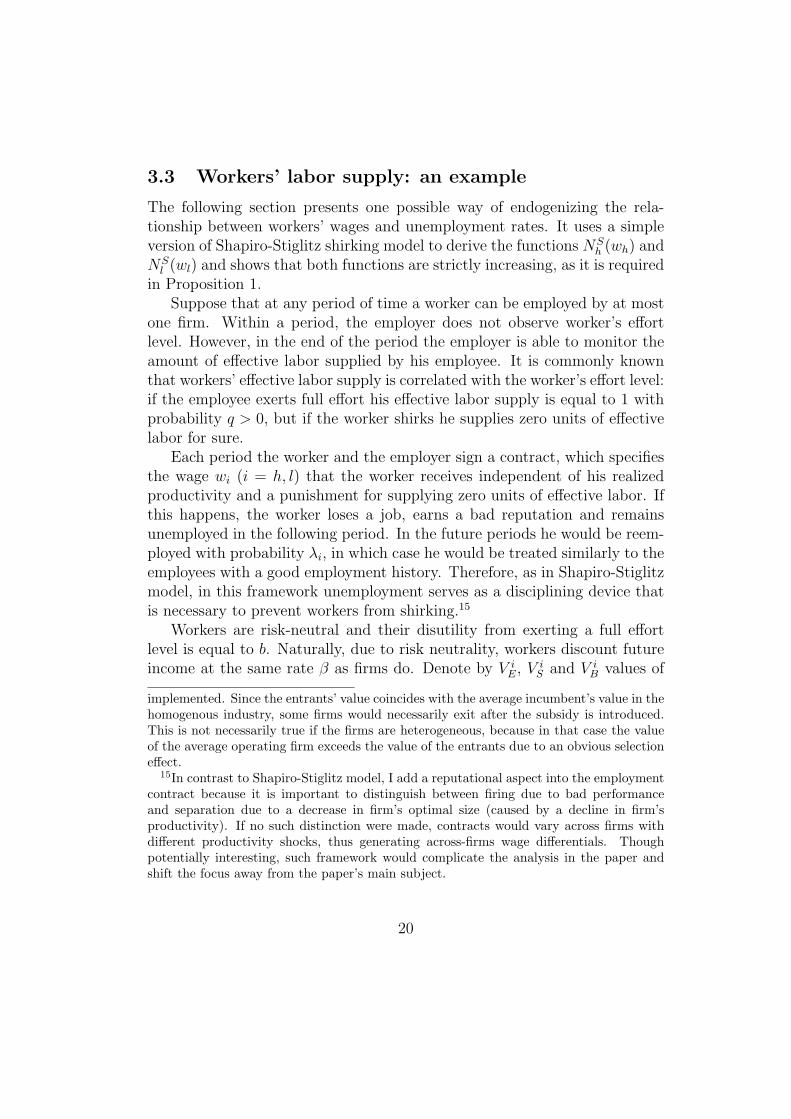
The following section presents one possible way of endogenizing the rela-tionship between workers’ wages and unemployment rates. It uses a simpleversion of Shapiro-Stiglitz shirking model to derive the functions NS

h (wh) andNS

l (wl) and shows that both functions are strictly increasing, as it is requiredin Proposition 1.

Suppose that at any period of time a worker can be employed by at mostone firm. Within a period, the employer does not observe worker’s effortlevel. However, in the end of the period the employer is able to monitor theamount of effective labor supplied by his employee. It is commonly knownthat workers’ effective labor supply is correlated with the worker’s effort level:if the employee exerts full effort his effective labor supply is equal to 1 withprobability q > 0, but if the worker shirks he supplies zero units of effectivelabor for sure.

Each period the worker and the employer sign a contract, which specifiesthe wage wi (i = h, l) that the worker receives independent of his realizedproductivity and a punishment for supplying zero units of effective labor. Ifthis happens, the worker loses a job, earns a bad reputation and remainsunemployed in the following period. In the future periods he would be reem-ployed with probability λi, in which case he would be treated similarly to theemployees with a good employment history. Therefore, as in Shapiro-Stiglitzmodel, in this framework unemployment serves as a disciplining device thatis necessary to prevent workers from shirking.15

Workers are risk-neutral and their disutility from exerting a full effortlevel is equal to b. Naturally, due to risk neutrality, workers discount futureincome at the same rate β as firms do. Denote by V i

E, V iS and V i

B values of

implemented. Since the entrants’ value coincides with the average incumbent’s value in thehomogenous industry, some firms would necessarily exit after the subsidy is introduced.This is not necessarily true if the firms are heterogeneous, because in that case the valueof the average operating firm exceeds the value of the entrants due to an obvious selectioneffect.

15In contrast to Shapiro-Stiglitz model, I add a reputational aspect into the employmentcontract because it is important to distinguish between firing due to bad performanceand separation due to a decrease in firm’s optimal size (caused by a decline in firm’sproductivity). If no such distinction were made, contracts would vary across firms withdifferent productivity shocks, thus generating across-firms wage differentials. Thoughpotentially interesting, such framework would complicate the analysis in the paper andshift the focus away from the paper’s main subject.

20

(i) being employed and exerting full effort; (ii) being employed and shirking;(iii) being unemployed due to having bad reputation, i = h, l. Formally,these values are related to each other in the following way:

V iE = wi − b + β[ q V i

E + (1− q)V iB ],

V iS = wi + βV i

B,

V iB = β[ λi V

iE + (1− λi)V

iB ].

(11)

If the employment contract is designed properly, workers never decide toshirk, i.e. the incentive constraint V i

E ≥ V iS must be satisfied implying that

βq(V iE − V i

B) ≥ b. (12)

Obviously, in a competitive labor market the incentive constraint should besatisfied with equality. Combining (12) with the first and the last equationsfrom (11) results in

wi =b

βq(1 + βλi). (13)

In the steady state, λi determines the unemployment rate ui among i−typeworkers. Recalling that only workers with bad reputation experience diffi-culties finding new job after being fired, it is obvious that

1− ui = (1− q)(1− ui) + λiui. (14)

Together with (13), the above equation implies that

ui =β(1− q)

βq wi/b− 1 + β(1− q). (15)

Correspondingly, total employment level of the workers of type i is equal to

NSi (wi) = Ni(1−ui) = Ni

(1− β(1− q)

βq wi/b− 1 + β(1− q)

), i = l, h, (16)

where Ni is the total number of workers of type i living in the economy.Note that NS

i (wi) is a strictly increasing function, as it was required inProposition 1. In addition, (16) implies that unemployment rate amongunskilled workers is higher than unemployment rate among skilled workersbecause the condition wh > wl is necessary to generate positive demand forunskilled labor.

21

Finally, it is also necessary to account for the fact that a fraction 1 − qof firms’ employees fail to supply any effective labor. This is easily correctedby modifying firms’ production function in the following way:

f(l) = f(ql).

Since such transformation preserves all the stipulated above properties of theproduction function, all the preceding results remain valid for f(l).

4 Numerical Analysis

This Section presents the results of a simulation exercise illustrating that,while evaluating the expected policy’s outcomes, it is important to take intoconsideration the structure of the production sector. First, it might be crucialto account for a potential change in the number of operating firms if the entryinto the industry is competitive. Second, a heterogeneity between youngand mature firms is also likely to play an important role in policy analysisbecause it can aggravate the policy’s adverse effect on the number of existingfirms. The numerical example below shows that overlooking any of thesetwo aspects may generate wrong predictions about the expected effects ofthe subsidy program.

4.1 Calibration procedure

The first part of this Section describes the calibration procedure. The pa-rameter values are chosen in such a way that the properties of the free-entryequilibrium allocation are consistent with the data on firms’ growth and sur-vival, amount of employer-provided training as well as the distribution ofworkers’ wages and unemployment rates. Table 1 lists all the exogenous pa-rameters of the model together with the data sources that are used to pindown the parameters’ values.

A time period is equal to one year, thus the time preference rate is setto β = 1/(1 + r) = 0.9524, where r = 0.05 stands for the annual interestrate. In order to set the parameters of the labor supply functions, I usethe relationship (15) between the workers’ wage and unemployment rates, wi

and ui, so that their equilibrium values match the distributions of wages andunemployment levels across workers with different skills.

22

Nickell and Bell (1996) classify US workers into two groups, with high andlow education, and report that: (i) the wages of more educated workers are1.51 times higher than the wages of the workers with relatively low education;(ii) unemployment rates among workers with high and low education areequal to 3% and 11% respectively; (iii) the average unemployment rate isequal to 6%16. Normalizing b = 1 and using (15), it is easy to derive thatq = 0.9734 would generate the equilibrium unemployment rates consistentwith the above observations. For this value of q, the equilibrium wages shouldbe equal to wh = 1.96 and wl = 1.3.17

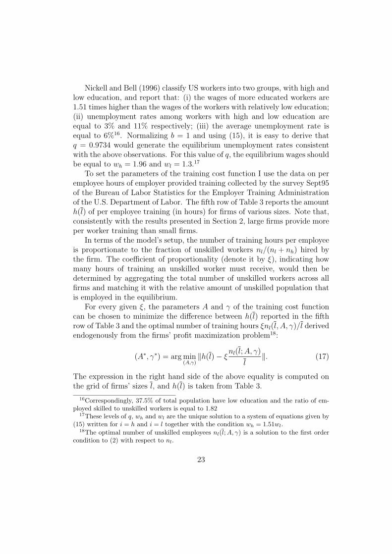
To set the parameters of the training cost function I use the data on peremployee hours of employer provided training collected by the survey Sept95of the Bureau of Labor Statistics for the Employer Training Administrationof the U.S. Department of Labor. The fifth row of Table 3 reports the amounth(l) of per employee training (in hours) for firms of various sizes. Note that,consistently with the results presented in Section 2, large firms provide moreper worker training than small firms.

In terms of the model’s setup, the number of training hours per employeeis proportionate to the fraction of unskilled workers nl/(nl + nh) hired bythe firm. The coefficient of proportionality (denote it by ξ), indicating howmany hours of training an unskilled worker must receive, would then bedetermined by aggregating the total number of unskilled workers across allfirms and matching it with the relative amount of unskilled population thatis employed in the equilibrium.

For every given ξ, the parameters A and γ of the training cost functioncan be chosen to minimize the difference between h(l) reported in the fifthrow of Table 3 and the optimal number of training hours ξnl(l, A, γ)/l derivedendogenously from the firms’ profit maximization problem18:

(A∗, γ∗) = arg min(A,γ)

‖h(l)− ξnl(l; A, γ)

l‖. (17)

The expression in the right hand side of the above equality is computed onthe grid of firms’ sizes l, and h(l) is taken from Table 3.

16Correspondingly, 37.5% of total population have low education and the ratio of em-ployed skilled to unskilled workers is equal to 1.82

17These levels of q, wh and wl are the unique solution to a system of equations given by(15) written for i = h and i = l together with the condition wh = 1.51wl.

18The optimal number of unskilled employees nl(l;A, γ) is a solution to the first ordercondition to (2) with respect to nl.

23

In turn, ξ is chosen to match the fraction of high skilled workers employedin the equilibrium with the one observed in the data. Given the wage levelswh and wl,

NDh (wh, wl, λ)

NDl (wh, wl, λ)

=

∑i µin

ih∑

i µinil

=Nh(1− uh)

Nl(1− ul)= 1.82, (18)

where {µi} stands for the observed in the data size distribution of firms(reported in the third row of Table 3), and the last number is taken from theestimations of Nickell and Bell (1996)19. It is easy to verify that the secondterm in the above equality is increasing in ξ if ξnl(l, A, γ)/l approximatesh(l) well enough. Thus ξ is well determined by the condition (18).

Therefore, using (17) and (18), I find that γ = 0.8249, A = 0.1352 andξ = 30.5 produce the best (in terms of (17)) approximation of the trainingfunction if the equilibrium wages are equal to wh = 1.96 and wl = 1.3.20 Thecorresponding optimal training hours derived from the model are reported inthe last row of Table 3.

Further, the vector of firms’ productivity shocks s is fixed in such a waythat the grid vector of firms’ possible sizes l is derived endogenously fromfirms’ maximization problem (i.e., it solves the first order condition to (2)with respect to l). Then the empirical evidence on firms’ growth and exitrates (summarized in the third and forth rows of Table 3) is used to set thevalues of the transition matrix Q. In turn, the distribution of entrants’ pro-ductivity shocks is determined as a solution to (6), where the equilibrium sizedistribution {µi} of firms is taken from the data.21 The corresponding valuesof the productivity shocks, the transition matrix Q and the distribution ofentrants G are reported in Table 2. Chosen in this way G implies that allthe entrants, who account for 35% of all incumbent firms, are responsiblefor 19% of total industry’s output (Dunne, Roberts and Samuelson (1988)

19See footnote 1520These computations are made for the production function f(l) = lα, in which α = 0.64

corresponds to the labor share of output. It is easy to see from the first order conditionsto the firm’s problem that the total firm’s expenditures on workers’ wages are equal towhl− (wh−wl)nl = sf ′(l)l = αf(l). Note that for this pair (α, γ) the second statement ofLemma 4 holds as long as wl/wh ≤ 0.80 (while in the benchmark equilibrium allocationwl/wh = 0.66).

21As it has been noted before, µλ is homogenous of degree 1 in λ, thus implying thatthe entrants’ distribution G, if found as solution to (6), is invariant in λ. Therefore λ = 1can be used to set G in this calibration exercise.

24

report this number being equal to 15.2% in the US manufacturing). Thismeans that, on average, entrants are significantly smaller than older firms:in the model the average entrants’ number of employees constitutes only 32%of the average employment of incumbent firms.

At the last stage, the entry cost η is set to satisfy the free entry conditiongiven that the equilibrium wages coincide with the obtained earlier valueswh = 1.96 and wl = 1.3. In the economy with the parameter levels definedabove, the entry cost η is equal to 100.6, which constitutes 29% of the valueof the average incumbent firm.

Finally, it has been verified that for the parameter values listed in Table1 the economy has the unique free entry equilibrium, i.e. the system ofequations (9) and (5) has a unique solution bundle (wh, wl, λ). To summarize,in this equilibrium allocation, the average economy’s unemployment rate isequal to 6%, with unemployment rates among skilled and unskilled workersbeing equal to 3% and 11% respectively. Skilled workers’ wage is 1.51 timeshigher than the wage of their unskilled colleagues. The average incumbentfirm hires 76 workers, while the average entering firm employs 24 workers(32% of the incumbent firm’s size). The equilibrium distribution of firms andtheir growth and survival rates coincide precisely with the data reported inthe upper part of Table 2. The hours of employer-provided training derived inthe model for different firm sizes are also listed in Table 2. As can be noticed,they approximate very well their empirical counterpart. When measured interms of firms’ output, the smallest and the largest firms spend respectively1.1% and 3.6% of their total revenue on own employees’ training.

4.2 Policy analysis: the role of competitive entry

This Section compares the effects of targeted employment subsidies on equi-librium allocations in the fixed entry and free entry economies. Suppose thatin the absence of subsidies the two equilibria are identical and all their en-dogenous variables coincide with those of the benchmark economy calibratedin the previous Section. Now assume that the government subsidizes a frac-tion θ of unskilled workers’ wage. Figure 3 illustrates the most importantdifferences in the two economies’ responses to such subsidy program. It plotsthe stationary equilibrium levels of the average unemployment rates and thenumber of operating firms for different levels of subsidies. The results for thefree entry equilibrium are plotted with solid line.

In a fixed entry equilibrium, the number of firms is fixed exogenously

25

at a given level (normalized to 1), thus a dashed line on the right panel ofFigure 3 is completely flat. In contrast, the number of firms in a free entryequilibrium adjusts as the subsidy rate varies: the bigger is the subsidy rate,the fewer firms operate in the industry because the increased tax pressurereduces the value of entrants and discourages start ups.

The more striking is the difference in the behavior of average unemploy-ment rates in the two economies illustrated on the left panel of Figure 3. Ina fixed entry equilibrium, the fraction of the economy’s employed populationincreases as the subsidy rate rises. However, once we account for a generalequilibrium effect arising due to endogeneity of the number of firms, the re-lationship between the subsidy rate and the unemployment level becomesnon-monotone. A relatively small subsidy rate stimulates labor demand andhas a positive effect on economy’s employment. However, as the subsidybecomes sufficiently large (more than 30%), it has an adverse effect on thevalue of entrants, is accompanied by a massive exit of firms and, as a result,it drives up the average unemployment rate above its value in the benchmarkeconomy. Correspondingly, there exist a level of subsidy, which minimizesaggregate unemployment rate. In this economy it is equal to 17% and itreduces average unemployment from 6% to 5%.

Figure 4 provides a more detailed characterization of the economy’s re-sponse to the targeted employment subsidy program. It explains the de-scribed above differences in the behavior of unemployment rates by illustrat-ing how the new policy affects wage and unemployment rates of each group ofworkers. First, in accordance with (ii) of Lemma 4, wages and employmentlevels of both types of workers rise after the introduction of the subsidiesbecause the number of firms in the economy remains unaffected and, at eachindividual firm’s level, skilled and unskilled workers serve as complementarylabor inputs.

At the same time, in a fixed entry equilibrium the increased tax pressurepushes the after-tax value of entrants below the level of the entry cost η.That is why, in a free entry equilibrium , both wage levels should decreasecompared to their values in the fixed entry allocation in order to balance thefree entry condition. More formally, such wage reduction is driven by thedecrease in the aggregate labor demand stipulated by the exit of firms. Af-ter the equality in the free entry condition is established, the wage of skilledworkers falls below its benchmark level (correspondingly, unemployment rateof skilled workers rises), but the wage of unskilled workers still remains aboveits level in a not subsidized economy. Therefore, even though the two labor

26

types are complementary from the viewpoint of every individual firm, theybecome substitutes at the aggregate level: the targeted employment subsidyprogram stimulates labor demand for unskilled workers, but the total de-mand for skilled employees decreases due to a fall in the number of operatingfirms.22

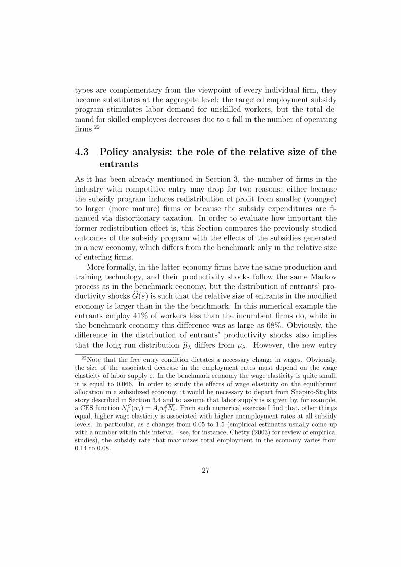
4.3 Policy analysis: the role of the relative size of theentrants

As it has been already mentioned in Section 3, the number of firms in theindustry with competitive entry may drop for two reasons: either becausethe subsidy program induces redistribution of profit from smaller (younger)to larger (more mature) firms or because the subsidy expenditures are fi-nanced via distortionary taxation. In order to evaluate how important theformer redistribution effect is, this Section compares the previously studiedoutcomes of the subsidy program with the effects of the subsidies generatedin a new economy, which differs from the benchmark only in the relative sizeof entering firms.

More formally, in the latter economy firms have the same production andtraining technology, and their productivity shocks follow the same Markovprocess as in the benchmark economy, but the distribution of entrants’ pro-ductivity shocks G(s) is such that the relative size of entrants in the modifiedeconomy is larger than in the the benchmark. In this numerical example theentrants employ 41% of workers less than the incumbent firms do, while inthe benchmark economy this difference was as large as 68%. Obviously, thedifference in the distribution of entrants’ productivity shocks also impliesthat the long run distribution µλ differs from µλ. However, the new entry

22Note that the free entry condition dictates a necessary change in wages. Obviously,the size of the associated decrease in the employment rates must depend on the wageelasticity of labor supply ε. In the benchmark economy the wage elasticity is quite small,it is equal to 0.066. In order to study the effects of wage elasticity on the equilibriumallocation in a subsidized economy, it would be necessary to depart from Shapiro-Stiglitzstory described in Section 3.4 and to assume that labor supply is is given by, for example,a CES function NS

i (wi) = Aiwεi Ni. From such numerical exercise I find that, other things

equal, higher wage elasticity is associated with higher unemployment rates at all subsidylevels. In particular, as ε changes from 0.05 to 1.5 (empirical estimates usually come upwith a number within this interval - see, for instance, Chetty (2003) for review of empiricalstudies), the subsidy rate that maximizes total employment in the economy varies from0.14 to 0.08.

27

cost η is chosen so that the benchmark equilibrium wages wh = 1.96 andwl = 1.30 are also consistent with the free entry equilibrium in the new econ-omy. That is why the corresponding unemployment rates coincide in the twoeconomies in the absence of subsidies.

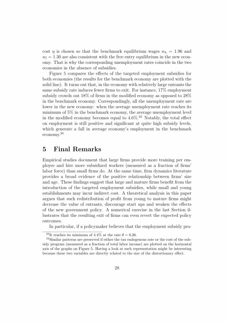
Figure 5 compares the effects of the targeted employment subsidies forboth economies (the results for the benchmark economy are plotted with thesolid line). It turns out that, in the economy with relatively large entrants thesame subsidy rate induces fewer firms to exit. For instance, 17% employmentsubsidy crowds out 18% of firms in the modified economy as opposed to 28%in the benchmark economy. Correspondingly, all the unemployment rate arelower in the new economy: when the average unemployment rate reaches itsminimum of 5% in the benchmark economy, the average unemployment levelin the modified economy becomes equal to 4.6%.23 Notably, the total effecton employment is still positive and significant at quite high subsidy levels,which generate a fall in average economy’s employment in the benchmarkeconomy.24

5 Final Remarks

Empirical studies document that large firms provide more training per em-ployee and hire more subsidized workers (measured as a fraction of firms’labor force) than small firms do. At the same time, firm dynamics literatureprovides a broad evidence of the positive relationship between firms’ sizeand age. These findings suggest that large and mature firms benefit from theintroduction of the targeted employment subsidies, while small and youngestablishments may incur indirect cost. A theoretical analysis in this paperargues that such redistribution of profit from young to mature firms mightdecrease the value of entrants, discourage start ups and weaken the effectsof the new government policy. A numerical exercise in the last Section il-lustrates that the resulting exit of firms can even revert the expected policyoutcomes.

In particular, if a policymaker believes that the employment subsidy pro-

23It reaches its minimum of 4.4% at the rate θ = 0.26.24Similar patterns are preserved if either the tax endogenous rate or the cost of the sub-

sidy program (measured as a fraction of total labor income) are plotted on the horizontalaxis of the graphs on Figure 5. Having a look at such representation might be interestingbecause these two variables are directly related to the size of the distortionary effect.

28

gram does not affect a number of operating firms or if he does not take intoaccount the large heterogeneity between young and mature firms observedin the data, he would expect that a 30% subsidy for hiring unskilled work-ers should have a positive impact on total employment. However, in themodelled economy this subsidy rate would actually decrease the total em-ployment level if one accounts for endogeneity of the number of operatingfirms as well as the realistic differences between young and mature firms.In addition, the simulation exercise presented in the papershows that therelationship between economy’s employment and subsidy rate is not mono-tone and that the same subsidy rate would generate more employment as thedegree of heterogeneity between young and mature firms increases.

In general, the main argument made of this work is not specific to thetargeted employment subsidy programs, but could be applied to many otherpolicies that are likely to have different impacts on the firms of different ages(firing taxes, start-up subsidies, etc.). Obviously, the described in the papergeneral equilibrium effect would be important only if a policy is implementedat a large scale (e.g., industry or economy level). For instance, in the nu-merical example discussed above the targeted group of workers is quite large,constituting about 35% of population. If the size of this group were muchsmaller, no significant effect on total employment would be observed.

A large number of empirical and theoretical studies discuss the sizes ofsubstitution and replacement effects associated with the introduction of var-ious subsidy programs. The goal of these works is to find out whether theseprograms create incentives for the firms to fire their regular workforce andhire instead subsidized workers. Traditionally, the replacement effects areevaluated by looking at the individual firms’ decisions. This paper describesa replacement mechanism that cannot be traced at the individual firms’ level.In response to the introduction of the subsidies, an average firm in the in-dustry hires more workers of each type. However, the total employmentlevel of skilled population may drop due to an endogenous decrease in thenumber of operating firms. Such aggregate replacement effect is likely to getbigger as the heterogeneity between young and mature firms gets more pro-nounced. From the econometric point of view, this observation suggests that(i) a structural general equilibrium model would produce a more accurateestimate of the replacement effects than a reduced-form approach and (ii)some measure of heterogeneity between young and mature firms could be animportant explanatory variable while estimating the effects of employmentsubsidy programs.

29

References

Alvarez, F. and M. Veracierto (2000). “Labor Market Policies in an Equilib-rium Search Model”. NBER Macro Annual, 265-316.

Bell, B., Blundell, R, and John Van Reenen (1999). “Getting the Unem-ployed back to Work: The Role of Targeted Employment Subsidies”. TheInstitute for Fiscal Studies Working Paper Series No. W99/12.

Bishop, John H. and Mark Montgomery (1986). “Evidence on Firm Par-ticipation in Employment Subsidy Programs”. Industrial Relations, Vol. 25,No. 1:56-64.

Blundell, K. and Costas Meghir (2001). “Active Labor Market Policy vsEmployment Tax Credit: Lessons from Recent UK Reforms”. Swedish Eco-nomic Policy Review, 8(2): 239-366.

Burtless, G. (1985). “Are targeted employment subsidies harmful? Evidencefrom a wage voucher experiment”. Industrial and Labor Relations Review39, 105-114.

Carling, K. and K. Richardson (2001). “The relative efficiency of labor mar-ket programs: Swedish experience from the 1990’s”. IFAU Working paper2001:2.

Calmfors, L., Forslund, M., and Maria Hemstrom (2001). “Does active labormarket policy work? Lessons from the Swedish experiences”. Swedish Eco-nomic Policy Review, 8(2): 63-124.

Chetty, Raj (2003). “A New Method of Estimating Risk Aversion”. NBERWorking paper 9988.

Davis, Steven and John Haltiwanger (1992). “Gross Job Creation, GrossJob Destruction, and Employment Reallocation”. The Quarterly Journal ofEconomics, 107(3):819-63.

Dunne, T., M. Roberts and L. Samuelson (1988). “Patterns of Firm Entryand Exit in U.S. Manufacturing Industries”. RAND Journal of Economics

30

19(4):495-515.

Dunne, T., M. Roberts and L. Samuelson (1989). “The Growth and Failureof U.S. Manufacturing Plants”. Quarterly Journal of Economics, 104 (1989),671-698.

Frazis, H., Gittleman, M, Horrigan, M., and Mary Joyce (1998). “Resultsfrom the 1995 Survey of Employer-Provided Training”. Monthly Labor Re-view Online. June 1998, Vol. 121, No. 6.

Hopenhayn, H.A. (1992). “Entry, exit, and firm dynamics in long run equi-librium”. Econometrica 60 (5), 1127-1150.

Hopenhayn, H.A. and R. Rogerson (1993). “Job turnover and policyevaluation: a general equilibrium analysis”. Journal of Political Economy101(5), 915-938.

Hui, W.T. and P.K. Trivedi (1986). “Duration dependence, targeted employ-ment subsidies and unemployment benefits”. Journal of Public Economics31, 105-129.

Kadlor, N. (1976). “Wage Subsidies as a Remedy for Unemployment”. Jour-nal of Political Economy, 44.

Katz, Lawrence (1996). “Wage Subsidies for the Disadvantaged”. NBERWorking Paper 5679.

Kambourov, Gueorgui and Iourii Manovskii (2002). “Rising Occupationaland Industry Mobility in the US: Evidence from the 1968-1993 PSID”.Manuscript.

Katz, Lawrence F. (1996). “Wage Subsidies for the Disadvantaged”. NBERWorking Paper 5679.

Martin, J., and David Grubb (2001). “What works and for whom: A reviewof OECD countries’ experience with active labor market policies”. SwedishEconomic Policy Review, 8(2): 11-60.

31

Mortensen, Dale T. and Christopher A. Pissarides (1998). “Taxes, Subsi-dies and Equilibrium Labor Market Outcomes”. CEPR Discussion paperNo. 2989.

Nickell, S., and Brian Bell (1996). “Changes in the Distribution of Wagesand Unemployment in OECD Countries”. American Economic Review 86(2):302-308.

Orszag, Michael J. and Dennis J. Snower (2002). “Unemployment Vouchersversus Low-Wage Subsidies“. IZA Discussion Paper Series No. 537.

Phelps, E. (1994). “Low-wage employment subsidies versus the welfarestate”. American Economic Review 84(2), 54-58.

Richardson, J. (1997). “Can Active Labor Market Policy work? Some Theo-retical Considerations”. Center for Economic Performance Discussion PaperNo. 331.

Shapiro, C. and Joseph Stiglitz (1984). “Equilibrium Unemployment as aWorker Discipline Device”. American Economic Review 74(3): 433-444.

Sianesi, B. (2001). “Differential effects of Swedish active labor market pro-grammes for unemployed adults during the 1990s”. IFAU Working Paper2001.

Veracierto, Marcelo (2000). “Employment Flows, Capital Mobility, and Pol-icy Analysis”. Federal Reserve Bank of Chicago Working Paper Series, No.2000-05.

32

6 Figures

0.96

0.98

1

1.02

1.04

1.06

1.08

1.1

1.12

0.96

0.98

1

1.02

1.04

1.06

1.08

1.1

1.12

0 0 productivity shock, s

Before tax, π*(s;wh,(1−θ)w

l) / π*(s;w

h,w

l) After tax, (1−τ)π*(s;w

h,(1−θ)w

l) / π*(s;w

h,w

l)

s* productivity shock, s

Figure 1: The effect of change in the unskilled workers’ wage wl on firmsprofit as a function of firms’ productivity level.

33

0 0.2 0.4 0.6 0.8 10

0.5

1

1.5

2

2.5

3

3.5

4

curvature of prod. function, α

curv

atur

e of

trai

ning

cos

t, γ

wl/w

h = 0.44

0 0.2 0.4 0.6 0.8 10

0.5

1

1.5

2

2.5

3

3.5

4

curvature of prod. function, α

curv

atur

e of

trai

ning

cos

t, γ

wl/w

h = 0.66

0 1 2 3 40.4

0.5

0.6

0.7

0.8

0.9

curvature of training cost, γ

Max

imal

rat

io w

l/wh

α = 0.44

0 0.2 0.4 0.6 0.8 10.4

0.5

0.6

0.7

0.8

0.9

1

curvature of prod. function, α

Max

imal

rat

io w

l/wh

γ = 0.83

Figure 2: Subsets of variables and parameters of the model for which thesufficient condition in (ii) of Lemma 4 holds: the shaded area on the toppanels correspond to the sets of (α, γ) for which wl/wh < 1− (1−α)/(1− γ)for wl/wh = 0.44 and wl/wh = 0.66 respectively; the bottom left panel graphsthe upper bound for wl/wh as a function of γ given that α = 0.64; the bottomright panel graphs the upper bound for wl/wh as a function of α given thatγ = 0.83.

34

0 0.05 0.1 0.15 0.2 0.250.03

0.035

0.04

0.045

0.05

0.055

0.06

0.065

0.07Unemployment rate

subsidy rate, θ0 0.05 0.1 0.15 0.2 0.25

0.4

0.5

0.6

0.7

0.8

0.9

1

1.1Number of firms

subsidy rate, θ

Figure 3: Comparison of the effects of targeted employment subsidies onaverage unemployment and the number of operating firms in the free entry( – ) and fixed entry ( – – ) economies.

35

0 0.05 0.1 0.15 0.2 0.250

0.01

0.02

0.03

0.04

0.05

0.06

0.07

0.08

0.09Unemployment, skilled

subsidy rate, θ0 0.05 0.1 0.15 0.2 0.25

0

0.02

0.04

0.06

0.08

0.1

Unemployment, unskilled

0 0.05 0.1 0.15 0.2 0.25

1.4

1.5

1.6

1.7

1.8

1.9

2

2.1Wage of skilled workers

0 0.05 0.1 0.15 0.2 0.251.3

1.35

1.4

1.45

1.5

1.55

1.6

1.65

1.7

Wage of unskilled workers

subsidy rate, θ

subsidy rate, θsubsidy rate, θ

Figure 4: Comparison of the effects of targeted employment subsidies onunemployment rates and wages in the free entry ( – ) and fixed entry ( – – )economies.

36

0 0.1 0.2 0.30.04

0.05

0.06

0.07

Unemployment rate

0 0.1 0.2 0.30.4

0.6

0.8

1

Number of firms

0 0.1 0.2 0.30

0.02

0.04

0.06

0.08

Unemployment, skilled

0 0.1 0.2 0.30

0.02

0.04

0.06

0.08

0.1

Unemployment, unskilled

0 0.1 0.2 0.3

1.4

1.6

1.8

2

Wage of skilled workers

0 0.1 0.2 0.31.3

1.35

1.4

1.45

1.5

1.55

1.6

Wage of unskilled workers

subsidy rate, θ

subsidy rate, θ subsidy rate, θ

subsidy rate, θ

subsidy rate, θ subsidy rate, θ

Figure 5: Comparison of the effects of targeted employment subsidies in theeconomies with small ( – ) and large ( – · – ) entrants.

37

7 Tables

The parameters of the model

Parameter Value Data to match

Time preference rate, β 0.9524 annual interest rate

Probability of supplying 0.9734 distribution of wagesfull labor, q and unemployment rates

Curvature of f(l), α 0.64 labor share of output

Multipl. of the training cost function, A 0.1352 per employee training

Curv. of the training cost function, γ 0.8249 per employee training

Per employee hrs of training, ξ 30.5 ratio of empl. levels

Vector of prod. shocks, s see Table 2 grid of firm sizes

Transition matrix, Q see Table 2 firms’ growth and exit

Distr. of entrants’ shocks, G see Table 2 size distr. of firms

Entry cost, η 101.6 average firm size

Table 1: The parameters of the model

38

Firms’ productivity shocks

Vector of productivityshocks, s

[0 9.3949 13.2989 17.2139 21.6806 25.0223

]

Distribution of shocksfor entrants, G

[0.3494 0.6086 0.0009 0.0368 0.0028 0.0015

]

Transition matrix, Q

1.0000 0 0 0 0 00.3796 0.5362 0.0655 0.0186 0 00.3460 0.0046 0.6213 0.0092 0.0190 00.2910 0 0.0081 0.6594 0.0324 0.00910.1910 0 0 0.0029 0.7685 0.03760.0500 0 0 0 0.0665 0.8835

Table 2: Values of firms’ productivity shocks, distribution of shocks for en-trants and transition matrix for incumbents.

39

Firms in the US manufacturing

Number of employees1, l 0-49 50-99 100-249 250-499 ≥ 500

Data:Fraction of firms2, µ 0.70 0.13 0.10 0.04 0.03Growth rates of survivors3 0.391 0.130 0.077 0.026 -Firm exit rates 0.379 0.346 0.291 0.191 -

Hours of training4, h(l) 3.34 8.2 11.39 14.56 16.6

Model:Fraction of firms 0.391 0.130 0.077 0.026 -Growth rates of survivors 0.391 0.130 0.077 0.026 -Firm exit rates 0.379 0.346 0.291 0.191 -

Hours of training, ξnl(l)/l 3.15 7.49 11.33 14.72 16.66

Notes:1In the numerical exercise it is assumed that firms’ productivity shocks can take sixpossible values, so that the corresponding employment levels fall in the middle if thesesize intervals, l = [25, 75, 175, 375, 600].2Source: Veracierto (2000), Table 2.3Source: This and the next rows are taken from Dunne, Roberts and Samuelson(1989).4Source: Frazis, Gittleman, Horrigan and Joyce (1998), Table 3, Column 4. Originallythe data are reported for firms with more than 50 employees, so the first number inthis row is obtained by extrapolation on the smaller levels of firms’ size under theassumption that firms with zero employees provide no training.

Table 3: Firms in the US manufacturing

40

8 Appendix

Proof of Lemma 1. Rewrite (2) as a function oh nl and l = nh + nl:

π∗(s; wh, wl) = maxl,nl

{sf(l)− wh(l − nl)− wlnl − c(nl, l − nl)} . (19)

To save on the notations, denote σ(nl, l) = c(nl, l− nl). Then the first orderconditions for the profit maximization problem (19) can be written as:

(l) : sf ′(l) = wh + σ2(nl, l)

(nl) : wh − wl = σ1(nl, l).(20)

Substituting (1) into the first order condition with respect to nl implies that

l =1 + γ

(wh − wl)A1+γ

(nl/l)γ

(1− nl/l)2+γ. (21)

The right hand side of the above equation is increasing in nl/l, so firm sizeand fraction of unskilled workers among its employees are positively related.Now substitute (21) into the expression for σ2(nl, l) and obtain that

σ2(nl, l) = −(1 + γ)

(nl

A(l − nl)

)γnl

A(l − nl)= −(wh − wl)

nl

l.

Then from the first order condition with respect to l it follows that

sf ′(l) = wh − (wh − wl)nl

l. (22)

Equations (21) and (22) form a system of equations with two unknowns, land nl

l∈ [0, 1]. It is straightforward to show (given concavity of f(·) that the

system has a unique solution (n∗l ,n∗ll∗ ). Consequently, (n∗l , l

∗) is the uniquesolution of the first order conditions (20).

The properties of the training cost function (c11 > 0, c12 < 0 and c22 > 0)insure that the second order condition is satisfied, i.e. the profit maximizationproblem (19) has a unique interior solution (n∗l (s; wh, wl), l

∗(s; wh, wl)). Thisproves (i) of Lemma 1. In addition, (21) and (22) imply that ∂l∗(s; wh, wl)/∂s >0, which, combined with the positive relationship between l and h/l derivedfrom (21), implies (ii) of Lemma 1.

41

In order to determine the sign of ∂l∂wl

, denote x = nl/l and differentiate

(21) and (22) with respect to wl:

sf ′′(l)∂l

∂wl

+ (wh − wl)∂x

∂wl

= x

1

l

∂l

∂wl

− 2x + γ

x(1− x)

∂x

∂wl

=1

wh − wl

.(23)

Solving the above system of equations we obtain that

∂l

∂wl

(1− x +2x + γ

x

sf ′′(l)lwh − wl

) =1

wh − wl

(1 +2x + γ

1− x)

∂x

∂wl

=x

wh − wl

− sf ′′(l)lwh − wl

∂l

∂wl

.

(24)

Correspondingly, ∂l∂wl

< 0 if and only if

1− x +2x + γ

x

sf ′′(l)lwh − wl

< 0. (25)

If f(l) = lα then

sf ′′(l)lwh − wl

=s(α− 1)f ′(l)

wh − wl

= (1− α)(x− wh

wh − wl

), (26)

where the last equality is obtained from (22). Therefore, inequality (25)holds if and only if

1− x + (2 +γ

x)(1− α)(x− wh

wh − wl

) < 0. (27)

The fraction x = nl/l lies within (0, 1) interval. As x → 0, the left handside of the above inequality is negative. At x = 1, it collapses to a negativeexpression (1 − α)(2 + γ)(1 − wh

wh−wl). Further, a simple algebraic exercise

verifies that if the left hand side of (27) has a local maximum point withinthe interval (0, 1), the value at this point is always negative.

In order to show that (iv) holds it is enough to prove that ∂2π∗(s; wh, wl)/∂wl∂s <0. Substituting (22) into the expression for the profit implies that

π∗(s; wh, wl) = sf(l)− slf ′(l)− c(nl, l).

42

Differentiating it with respect to s suggests that

∂π∗

∂s= f(l)− lf ′(l)− slf ′′(l)

∂l

∂s− (wh − wl)

∂nl

∂s− (sf ′(l)− wh)

∂l

∂s. (28)

Equation (22) allows to express ∂nl/∂s as a function of l and ∂l/∂s:

(wh − wl)∂nl

∂s= wh

∂l

∂s− lf ′(l)− s(f ′(l) + f ′′(l)l)

∂l

∂s.

Substituting the above expression into (28) implies that ∂π∗∂s

= f(l). Then∂2π∗∂s∂wl

= f ′(l) ∂l∂wl

, which is less than zero if and only if ∂l∂wl

< 0.

Finally, it is straightforward to see that lims→0∂2π∗∂π∂s

(s; wh, wl) = 0, whichimplies (iv) of Lemma 1.

Q.E.D

Proof of Lemma 2. By the Blackwell Sufficient Condition, the func-tional operator in the right hand side of the Bellman equation (3) is a contrac-tion and thus, by Contraction Mapping Theorem, (3) has a unique solutionV (s; wh, wl). A standard recursive argument, together with Assumption 1implies that V (s; wh, wl) is a continuous and increasing function in s.

Since s = 0 is an absorbing state, lims→0

∫V (s′; wh, wl)Q(s, ds′) = V (0; wh, wl).

Therefore, V (0; wh, wl) = π∗(0; wh, wl) + 11+r

max{0, V (0; wh, wl)}, which im-plies that V (0; wh, wl) = 0. By monotonicity of V (s; wh, wl) in its first argu-ment,

V (s; wh, wl) ≥ π∗(s; wh, wl) + 0 > 0,

for all s > 0. This completes the proof of (i) of Lemma 2.Note that

∫V (s′; wh, wl)Q(s, ds′) > 0 for all s > 0, thus for any positive s

(3) can be rewritten as

V (s; wh, wl) = π∗(s; wh, wl) +1

1 + r

∫V (s′; wh, wl)Q(s, ds′). (29)

Differentiating (29) with respect to wl, applying monotonicity of Q(s, S) andusing (iii) of Lemma 1, verifies (ii) of Lemma 2 in a straightforward way. In

addition, from Assumptions 1 and 2, combined with lims→0∂2π∗(s;wh,wl)

∂s∂wh= 0

it follows that (iii) of Lemma 2 holds.

43

Finally, it is easy to see that the value function Vτ (s; wh, wl) = (1−τ)V (s; wh, wl)solves the Bellman equation (4). Thus

lims→0

Vτ (s; wh, wl −∆)

V (s; wh, wl)= (1− τ) lim

s→0

V (s; wh, wl −∆)

V (s; wh, wl)= 1− τ < 1.

Employing continuity and monotonicity of both V (s; wh, wl) and Vτ (s; wh, wl)allows to conclude that (iv) of Lemma 2 holds.

Q.E.D

Proof of Lemma 3 is similar to Hopenhayn (1993).

Proof of Lemma 4. Since wl and wh have no impact on the shape ofthe stationary distribution µλ, it is enough to show that similar propertieshold for the individual firms’ hiring policies. The structure in the proofis reminiscent with the one used in the proof of (iii) in the first Lemma:differentiating (21) and (22) with respect to wh (or wl) produces the systemof two equations with two unknown partial derivatives. Solving this systemallows to determine the derivatives’ signs.

First, note that∂nl

∂wl

=∂x

∂wl

l +∂l

∂wl

x, (30)

where x = nl/l. Equations (21) and (22) have been already differentiatedwith respect to wl in (24). Substituting them into (30) implies that

∂nl

∂wl

=l

wh − wl

[1 + x + γ

1− x + 2x+γx

sf ′′(l)lwh−wl

(x− sf ′′(l)l

wh − wl

)+ x

]. (31)

Rearranging the terms in the right hand side of the above expression andusing inequality (25), which has been established earlier as a necessary con-dition for ∂l

∂wl< 0, one easily derives that ∂nl

∂wl< 0 if and only of

2x + γx− sf ′′(l)lwh − wl

> 0.

Concavity of f(l) implies that the above inequality is always true. Thus∂nl

∂wl< 0 holds for every operating firm, and, a similar property is satisfied for

the aggregate demand,∂ND

l (wh,wl,λ)

∂wl< 0.

44

In order to prove the second part of the statement (i) of Lemma 4, dif-ferentiate (21) and (22) with respect to wh:

∂x

∂wh

=1− x

wh − wl

− sf ′′(l)wh − wl

∂l

∂wh

γ + 2x

x(1− x)

∂x

∂wh

=1

wh − wl

+1

l

∂l

∂wh

.

(32)

This allows to express ∂nh

∂whas

∂nh

∂wh

=l(1− x)

wh − wl

(γ + x)(1− x + sf ′′(l)lwh−wl

)− x(1− x + γ+2xx

sf ′′(l)lwh−wl

)

1− x + γ+2xx

sf ′′(l)lwh−wl

.

As it has been shown earlier, the denominator of the right hand side isnegative since ∂l

∂wl< 0. Thus ∂nl

∂wlis negative if and only if the nominator

of right hand side is positive. One can easily verify that this is true byrearranging the terms of the nominator and showing that it collapses to apositive expression γ(1 − x) − x sf ′′(l)l

wh−wl. This completes the proof of (i) of

Lemma 3.Finally, ∂nh

∂wl= ∂l

∂wl(1−x)− ∂x

∂wll. Substitute into this equation the expres-

sions for ∂l/∂wl and ∂x/∂wl that solve (24). This results in

∂nh

∂wl

=l(1− x)

wh − wl

(1 +

2x + γ

1− x

)1− x + sf ′′(l)l

wh−wl

1− x + 2x+γx

sf ′′(l)lwh−wl

− xl

wh − wl

.

Rearranging the terms in the above equation and using the inequality (25) we

conclude that ∂nh/∂wl < 0 if and only if 1 + γ + sf ′′(l)lwh−wl

> 0. Substitute (26)

into the above inequality to obtain that it holds for every x if wl

wh< 1− 1−α

1+γ.

Therefore, (ii) of Lemma 3 is also verified.

Q.E.D

Proof of Proposition 1 is straightforward and is summarized in thediscussion following the proposition.

45