E2e Working Paper 015

Does Better Information Lead to Better Choices? Evidence from Energy-Efficiency Labels

Lucas Davis and Gilbert Metcalf

November 2015

E2e is a joint initiative of the Energy Institute at Haas at the University of California, Berkeley, the Center for Energy and Environmental Policy Research (CEEPR) at the Massachusetts Institute of Technology, and the Energy Policy Institute at Chicago, University of Chicago. E2e is supported by a generous grant from The Alfred P. Sloan Foundation. The views expressed in E2e working papers are those of the authors and do not necessarily reflect the views of the E2e Project. Working papers are circulated for discussion and comment purposes. They have not been peer reviewed.

Revised version published in Journal of Association of Environmental and Resource

Economists, 2016, 3(3), 589-625.

* (Davis) Haas School of Business, University of California, Berkeley; Energy Institute at Haas; and National Bureau of Economic Research. Email: ldavis@haas.berkeley.edu. (Metcalf) Department of Economics, Tufts University and National Bureau of Economic Research. Email: gmetcalf@tufts.edu. We are grateful to Hunt Allcott, Stefano DellaVigna, Matthew Harding, Sébastien Houde, Kelsey Jack, and seminar participants at Iowa State, Illinois, UC Berkeley, Harvard, and the NBER for helpful comments. We also thank Poom Nukulkij at GfK for his work on the experiment. Data collected by Time-sharing Experiments for the Social Sciences, NSF Grant 0818839, Jeremy Freese and James Druckman, Principal Investigators. This RCT was registered in the American Economic Association Registry for randomized control trials under Trial number 560. The authors have not received any financial compensation for this project nor do they have any financial relationships that relate to this research.

Does Better Information Lead to Better Choices? Evidence from Energy-Efficiency Labels

Lucas W. Davis* UC Berkeley and NBER

Gilbert E. Metcalf

Tufts University and NBER

November 2015

Abstract

Information provision is a key element of government energy-efficiency policy, but the information that is provided is often too coarse to allow consumers to make efficient decisions. An important example is the ubiquitous yellow “EnergyGuide” label, which is required by law to be displayed on all major appliances sold in the United States. These labels report energy cost information based on average national usage and energy prices. We conduct an online stated-choice experiment to measure the potential welfare benefits from labels tailored to each household’s state of residence. We find that state-specific labels lead to significantly better choices. Consumers choose to invest about the same amount overall in energy-efficiency, but the allocation is much better with more investment in high-usage high-price states and less investment in low-usage low-price states.

Key Words: Energy-Efficiency, Inattention, Information Provision, Energy Demand, EnergyGuide JEL: D12, H49, Q41, Q48

1

1. Introduction

Information provision is a key element of government energy-efficiency policy.

An important example is the ubiquitous yellow “EnergyGuide” label, which is required

by law to be displayed on all major appliances sold in the United States. Similarly, new

cars and trucks sold in the United States must display information about vehicle fuel

efficiency and an estimate of annual gasoline expenditures. Over 40 countries worldwide

have some sort of energy-efficiency labelling requirements (CLASP, 2014).

This information is intended to help consumers make better decisions. However,

in many cases government-mandated labels do not provide accurate information

necessary for consumers to make efficient decisions. In particular, most labels report only

very coarse information based on national average energy prices and typical national

usage. In practice, energy prices and typical usage vary substantially, so the labels

provide information that is highly inaccurate for many consumers.

The objective of our project is to evaluate the potential welfare benefits from

providing more accurate information. We focus on room air conditioners because they

are a particularly lucid example. Within the lower 48 U.S. states we show that annual

cooling hours range by a 9:1 ratio, while electricity prices vary by more than a 2:1 ratio.

As a result, typical operating costs vary widely, from $28 per year in Washington state, to

$316 per year in Florida. Despite these very large differences in operating costs,

consumers in all states see the exact same EnergyGuide label.

We designed and implemented an online stated-choice experiment to measure

how consumer decisions would change with information tailored to each household’s

state of residence. We find that better labels indeed lead to better choices. When

presented with more accurate information, the average energy-efficiency of selected air

conditioners stays about the same, but the allocation is much better. Households facing

low energy prices and low expected usage invest less in energy-efficiency, while

households facing high energy prices and high expected usage invest more. This

reallocation leads to lower lifetime costs – defined as the sum of purchase price plus

present discounted value of energy costs – for both types of households.

2

The implied aggregate savings are substantial. State-specific labels decrease

lifetime cost by an average of $11.60 per air conditioner. U.S. consumers purchase more

than 4 million room air conditioners each year, so the implied aggregate cost savings

exceed $50 million annually. Moreover, our results suggest that state-specific labels

would improve decision-making not just for room air conditioners, but for a whole host

of residential appliances.

We then provide additional analysis and evidence aimed at better understanding

the mechanisms underlying our results. We find that immediately after the experiment

most participants are unable to correctly answer basic questions about the information

they have just seen. Most do not know whether the labels they just saw were based on

national or state energy prices, nor do they know how energy prices or appliance usage in

their state compares to the national average.

Overall, the evidence points to people taking the information in these labels as

given without analyzing it carefully. Daniel Kahneman (2011) has referred to this kind of

decision making as WYSIATI: “What You See Is All There Is.” The content of the labels

changes participants’ decisions, so it is not that they are ignoring this information

completely. But they appear not to be exerting the additional effort that would be

required to understand what this information means nor are they spontaneously

transforming this information to take local conditions into account.

Our paper differs from most previous studies of energy-efficiency. While there is

an extensive theoretical and empirical literature on the economic determinants of

investments in energy-efficient capital, there is little that has taken an explicit

experimental approach. None of the work to date has focused on the efficiency cost of

inaccurate information provided to consumers as this study does.1,2 Our paper

complements a growing broader literature that shows that customized information can 1 Studies focusing on consumer choice of energy efficient capital include Hausman (1979), Dubin and McFadden (1984), Metcalf (1994), Revelt and Train (1998), Metcalf and Hassett (1999), and Davis (2008) among others. See Gillingham, Newell, and Palmer (2009) and Gillingham and Palmer (2014) for recent surveys. 2 Two related studies perform online experiments using the same nationally-representative panel that we employ. Newell and Siikamaki (2014) analyze optimal EnergyGuide label design while Allcott and Taubinsky (2015) measure the effect of information provision on willingness-to-pay for energy-efficient lightbulbs. Neither study considers the role of inaccurate information provided to consumers.

3

significantly improve education, health, and finance-related choices (see, e.g., Hastings

and Weinstein, 2008; Bertrand and Morse, 2011; Kling et al., 2012; and Hoxby and

Turner, 2013).

It is worth emphasizing that our evidence comes from a stated-choice experiment.

The highly-stylized setting allows us to eliminate many of the factors that complicate

these decisions in real-world settings. This facilitates analysis and interpretation, but it

also may lead participants to focus more on labels than they otherwise would. One

approach to validating our results is to look for complementary evidence from actual

choices. Examining nationally-representative data from air conditioner purchases, we

find no evidence of a positive correlation between operating costs and investments in

energy-efficiency. Although this doesn’t tell us how much choices would change with

better information, it provides some corroboration for other results in the paper about the

lack of effectiveness of current labels.

The paper proceeds as follows. Section 2 provides background information, and

makes the case for why better information might matter. Section 3 describes our online

experiment. Sections 4 and 5 provide the main results and additional analysis. Section 6

offers concluding comments.

2. Background

A. Previous Research

Economists have long been interested in how consumers make energy-related

decisions. Hausman (1979) and Dubin and McFadden (1984) model durable good

purchase decisions as a household production problem with a tradeoff between purchase

price and operating cost. Following these seminal studies, much of the literature has

focused on whether or not consumers undervalue operating cost when making these

tradeoffs (see, e.g., Metcalf 1994 and Metcalf and Hassett 1999). The most recent

evidence comes from vehicle purchases and indicates that consumers do not undervalue

(Busse, Knittel, and Zettelmeyer, 2013) or modestly undervalue operating costs (Allcott

and Wozny, 2014).

Another recent strand in the literature has aimed at understanding specific

4

behavioral biases in energy-related decisions. Allcott (2011a) and Allcott (2013)

examine “MPG Illusion’’, the idea that consumers may not understand the non-linear

relationship between miles-per-gallon and motor vehicle fuel consumption. Camilleri and

Larrick (2014) test whether vehicle preferences are affected by the scale in which fuel

economy information is expressed, for example, gallons per 100 miles versus gallons per

1000 miles. Lastly, Allcott and Taubinsky (2015) and Allcott and Sweeney (2014) test

for biased beliefs and imperfect information by measuring the effect of information

provision on demand for energy-efficient lightbulbs and hot water heaters, respectively.

There are also studies that examine the effect of environmental messaging like

Energy Star Certification (e.g. Newell and Siikamaki (2014); Houde (2014b)) and

“normative” letter grades for the energy-efficiency characteristics of products (e.g.

Brounen and Kok (2011)).3 The evidence shows that people respond to these non-price

interventions though it is not always clear if this is because they trigger “warm glow”

responses or because they are indirectly providing information about private costs.

Finally, there is a group of papers that study the effect of peer comparisons.

Learning about how your electricity consumption compares to your neighbors tends to

significantly reduce consumption, both in the short-run and long-run. See, for example,

Ayres, Raseman, and Shih (2009), Allcott (2011b), and Allcott and Rogers (2014).

We see what we are doing as quite different. We are not studying consumers’

undervaluation of energy costs, nor are we studying a specific behavioral bias like MPG

illusion. Moreover, we have designed our experiment explicitly to exclude any

environmental messaging or peer comparisons. Instead, we are focused sharply on the

quality of the information that is publicly provided, and we want to ask whether better

tailoring this information to consumers’ characteristics can lead to more efficient choices.

B. U.S. Energy Labeling Requirements

EnergyGuide labels must be displayed on all major appliances sold in the United 3 Newell and Siikamaki (2014) is similar to our study in that it uses an online stated-choice experiment to evaluate components of EnergyGuide labels. In addition to comparing choices with and without Energy Star certification, they randomly include or exclude information about carbon dioxide emissions, normative letter grades, and other elements of label design. They do not, however, vary the operating cost information itself or explore information that is tailored to the participant’s local usage or prices.

5

States. As of 2015, this includes clothes washers, dishwashers, refrigerators, freezers,

televisions, water heaters, window air conditioners, central air conditioners, furnaces,

boilers, heat pumps, and pool heaters. Collectively, these appliances account for over

60% of residential energy consumption, and 13% of total U.S. energy consumption.4

Energy efficiency labels have existed since the first energy crisis in the mid-

1970s. France mandated labels for a variety of appliances in 1976 and Japan, Canada,

and the United States followed soon after (Wiel and McMahon, 2001).5 The Energy

Policy and Conservation Act of 1975 mandated labels for certain appliances beginning in

1980. Changes to the labeling program were made in the Energy Policy Act of 1992

which gave rise to the EnergyGuide labels in their current form.

The Federal Trade Commission (FTC) is charged with enforcing these labeling

requirements. The FTC provides templates on its website for manufacturers to use and

the Energy Labeling Rule in the Code of Federal Regulations provides samples of

acceptable labels (Federal Trade Commission, 2014).

Information provision requirements for vehicles are similar. Since 1977, all new

cars and trucks sold in the United States must display information about vehicle fuel

efficiency. Until recently, labels reported estimated city, highway, and combined fuel

efficiency in miles-per-gallon (MPG). Starting with model year 2013, new labels provide

additional information including estimated gallons per 100 miles, annual fuel cost, and

five year fuel cost savings compared the average new vehicle. The inclusion of gallons

per 100 miles brings the United States in line with the European Union which reports

liters per 100 kilometers.

Fuel economy labels on vehicles suffer from the same problem as do appliance

labels in using national energy prices to compute fuel savings and ignoring variation in

vehicle miles traveled across the states. Paradoxically, the improvement in fuel economy

4 According to U.S. DOE (2014a), Table A4, space heating, space cooling, water heating, refrigeration, clothes dryers, freezers, clothes washers, and dishwashers accounted for 62% of total residential energy consumption in 2012. These end-uses represented in 2012 a total of 12.5 quadrillion Btu compared to 95.0 quadrillion Btu from all sectors and sources in 2012. 5 Wiel and McMahon (2001) discuss the early motivation for energy labels. Thorne and Egan (2002) conduct qualitative interviews with focus groups about alternative graphical elements and other aspects of EnergyGuide label design.

6

labels on motor vehicles may exacerbate losses from inaccurate information on the labels.

When labels only reported miles per gallon, consumers had to undertake significant

mental computations to balance the cost savings from a more fuel efficient vehicle

against the higher purchase price (holding other attributes constant). The current labels

now report estimated five year cost savings for each vehicle relative to the fleet average.

Now it is more straightforward to balance cost savings from more efficient vehicles

against higher purchase price. But cost savings can differ significantly given differences

in average gasoline prices and driving patterns across states. Whether consumers will

make those mental adjustments is not clear.

C. Focus on Air Conditioning

More accurate labels could be important for many different appliance types but in

our experiment we focus specifically on room air conditioners. More than 25 million

American households own one or more room air conditioners so this is an appliance that

is of large intrinsic interest.6 It is also a particularly lucid example of an energy-efficiency

investment for which consumers face a clear tradeoff between purchase price and energy

costs, and for which operating costs vary substantially across states. Moreover, most

consumers install room air conditioners themselves, thereby avoiding any principal-agent

problem that arises when contractors are involved in selecting and installing equipment.

More broadly, residential air conditioning is of large and growing policy interest

nationwide because of the high level of energy consumption associated with it. In the

United States, there is air-conditioning in nearly 100 million homes (87% of homes), and

households spend an estimated $22 billion dollars annually on electricity for air-

conditioning.7 Table 1 shows that air conditioner usage is pervasive in all parts of the

country. The lowest share is in the West where one-third of households have no form of

air conditioning. The table also illustrates considerable variation in the shares of central

versus room air conditioning among those households with air conditioning with central

air conditioning dominating in all regions except the Northeast.

6 U.S. Department of Energy, Residential Energy Consumption Survey 2009. See Table HC7.1 “Air Conditioning in U.S. Homes”. 7 Data from U.S. Department of Energy (2009). See Table HC7.1 “Air Conditioning in U.S. Homes” and Table CE3.6 “Household Site End-Use Consumption in the U.S.”.

7

Figure 1 shows annual cooling hours by state from U.S. Department of Energy

(2014).8 This is the number of hours per year for which a household should expect to use

an air conditioner. On average, Americans face 1,265 cooling hours per year, but there is

enormous geographic variation. Within the continental United States average annual

cooling hours range from 310 in Maine to 2,771 in Florida, almost a 9:1 ratio.

Figure 2 shows average residential electricity prices by state for 2012 from U.S.

Department of Energy (2013a), Table 2.10. The average price is 12.4 cents per kilowatt

hour, but again there is substantial geographic variation. The lowest electricity prices in

2012 were in Louisiana (8.4 cents), while New York had the most expensive prices (17.6

cents), so more than a 2:1 ratio. Figure 2 is only showing variation in prices across states.

But there is variation within states across utilities as well. Using data from the 2013 EIA

Form 861, we computed the standard deviation of residential electricity prices by utility

across the United States. The standard deviation in prices across the country is 3.7 cents

per kWh. The standard deviation across states is 5.22 cents per kWh while the standard

deviation within states is only 2.7 cents per kWh. This much lower variation within states

suggests the potential for improving information with state-specific labels.

Annual operating cost for a room air conditioner depends on cooling hours and

electricity prices according to this simple equation,

(1)

Annual Operating Cost

(dollars)

=

Annual Cooling Hours

*

Electricity Price (dollars

per watt hour)

*

Size of Air Conditioner,

(BTUs)

/

Energy-Efficiency Ratio

of Air Conditioner

(BTUs per watt)

The “energy-efficiency ratio”, or EER, of an air conditioner is the ratio of the unit’s

cooling capacity (in BTUs) to its electricity consumption (in watts). The higher the EER,

the more energy-efficient the air conditioner. Figure 3 shows annual operating costs for a

medium-sized (10,000 Btu), medium-efficiency (10.0 EER) room air conditioner by state.

Operating costs vary widely across states, from $28 per year in Washington to $316 per

year in Florida, more than an 11:1 ratio. The geographic pattern reflects variation in both

8 U.S. Department of Energy (2014) reports annual cooling hours for room air conditioners for 218 U.S. cities. We aggregated to the state level taking a weighted average of cities within each state weighting by population.

8

cooling hours and electricity prices.

3. Experimental Design

A. Overview

Our experiment was implemented through Time-Sharing Experiments for the

Social Sciences (TESS), an NSF-funded program aimed at making it easier for academics

to run online experiments. TESS contracts with GfK (formerly “Knowledge Networks”)

a company that administers surveys and experiments using a nationally-representative

panel which they call the KnowledgePanel. This platform has been widely used by

economists, see, e.g., Allcott (2013), Allcott and Taubinsky (2015), and Newell and

Siikamaki (2014).

The KnowledgePanel is a nationally representative panel of some 55,000 adults

selected using random-digit dialing and address-based sampling (GfK, 2013).

Participants are provided with a computer and free internet service if they do not already

have it. From this panel, GfK constructs samples to respond to surveys and participate in

experiments on a wide variety of topics. Samples are constructed to represent the

underlying population of interest and upon completion of the survey or experiment,

study-specific sample weights are provided to ensure that the observable characteristics

of the final sample match the characteristics of the population of interest (GfK, nd). The

TESS-funded surveys put limits on sample size and the number of questions. For our

experiment, GfK asked 3,744 participants to take the survey, of whom 2,440 completed

the experiment (completion rate of 62.5 percent).

Participants in our experiment were asked to make three hypothetical purchase

decisions. Each decision involved selecting one of three room air conditioners that varied

by purchase price and expected annual energy cost. Participants were told that the three

air conditioners were otherwise identical except for these features. And, as we explain in

the appendix,we designed the choice sets carefully to maximize the precision of our

estimates.We designed the experiment as a simple randomized controlled trial with

participants randomly assigned to either the control group or the treatment group. During

the experiment, the only difference between these two groups was the labels that they

9

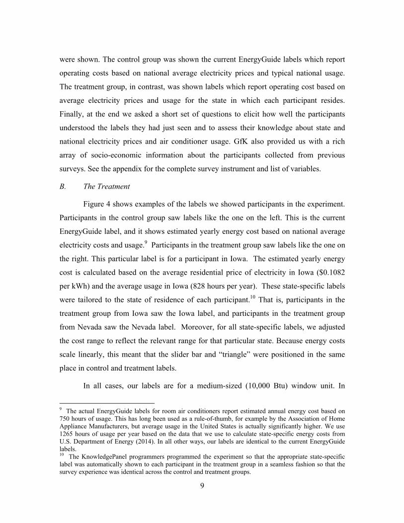
were shown. The control group was shown the current EnergyGuide labels which report

operating costs based on national average electricity prices and typical national usage.

The treatment group, in contrast, was shown labels which report operating cost based on

average electricity prices and usage for the state in which each participant resides.

Finally, at the end we asked a short set of questions to elicit how well the participants

understood the labels they had just seen and to assess their knowledge about state and

national electricity prices and air conditioner usage. GfK also provided us with a rich

array of socio-economic information about the participants collected from previous

surveys. See the appendix for the complete survey instrument and list of variables.

B. The Treatment

Figure 4 shows examples of the labels we showed participants in the experiment.

Participants in the control group saw labels like the one on the left. This is the current

EnergyGuide label, and it shows estimated yearly energy cost based on national average

electricity costs and usage.9 Participants in the treatment group saw labels like the one on

the right. This particular label is for a participant in Iowa. The estimated yearly energy

cost is calculated based on the average residential price of electricity in Iowa ($0.1082

per kWh) and the average usage in Iowa (828 hours per year). These state-specific labels

were tailored to the state of residence of each participant.10 That is, participants in the

treatment group from Iowa saw the Iowa label, and participants in the treatment group

from Nevada saw the Nevada label. Moreover, for all state-specific labels, we adjusted

the cost range to reflect the relevant range for that particular state. Because energy costs

scale linearly, this meant that the slider bar and “triangle” were positioned in the same

place in control and treatment labels.

In all cases, our labels are for a medium-sized (10,000 Btu) window unit. In

9 The actual EnergyGuide labels for room air conditioners report estimated annual energy cost based on 750 hours of usage. This has long been used as a rule-of-thumb, for example by the Association of Home Appliance Manufacturers, but average usage in the United States is actually significantly higher. We use 1265 hours of usage per year based on the data that we use to calculate state-specific energy costs from U.S. Department of Energy (2014). In all other ways, our labels are identical to the current EnergyGuide labels. 10 The KnowledgePanel programmers programmed the experiment so that the appropriate state-specific label was automatically shown to each participant in the treatment group in a seamless fashion so that the survey experience was identical across the control and treatment groups.

10

addition to reporting the estimated yearly energy cost in dollars, the label also reports the

unit’s EER, and further below, the label includes the language “Your cost will depend on

your utility rates and use.” Finally, the bottom of the label provides three bullets with

additional details. The first bullet explains that the cost range is based only on models

with similar capacity and characteristics. The second bullet explains how the energy cost

was calculated. This is important for our experiment, and we varied the text here

depending on treatment status. For the control group, the text reads, “Estimated energy

cost based on a national average electricity cost of 12.4 cents per kWh and national

average usage.” For the treatment group, the text reads, "Estimated energy cost based on

average electricity costs and usage for [State Name]." Finally, the last bullet points

consumers to the FTC website for more information.

C. Balance in Sample

Before moving on to results, we test for balance between the control and

treatment groups. Since treatment status was randomly assigned, we expect very similar

characteristics in the two groups. Table 2 reports mean characteristics for the control and

treatment groups as well as p-values from tests that the means are equal. We report

weighted means using the sampling weights that GfK constructed specifically for our

experiment. This socio-economic information including political party affiliation was

collected from the individuals in the KnowledgePanel by GfK during previous surveys.11

Not surprisingly, given the design of the experiment, we fail to reject equality of

means between the two groups for any of the socioeconomic characteristics. The p-

values of 1.0 for educational status, sex, and race reflect the fact that the experiment-

specific sampling weights are balancing on these attributes.12 The mean characteristics

also match national data quite well. For example, the proportion of households with

central air conditioners (65.5 and 67.5 percent) is similar to the national average from the 11 Political party affiliation is measured by GfK as "strong", "not strong", or "leans." We constructed indicator variables for Democratic and Republican affiliation based on whether each participant indicated "strong" or "not strong" support for a particular party. 12 The unweighted means are also very similar between the control and treatment groups. We also computed p-values for equality of means between the two groups with the unweighted data and we continue to find p-values in excess of 10 percent for the demographic and economic characteristics. In addition we ran a weighted regression of a treatment indicator variable on all the variables in Table 2. The F-statistic for the joint test that all the estimated coefficients are zero has a p-value of 0.75.

11

2009 Residential Energy Consumption Survey reported in Table 1 (63 percent). The

fraction of participants with high school and college degrees is also similar to data from

the U.S. Census Bureau.

Despite households being randomly assigned to control and treatment groups, the

average residential electricity price is slightly higher in the control group and statistically

significant at the 10 percent level. Consequently, average yearly energy costs are also

slightly higher in the control group, though this difference is not statistically significant.

We attribute these modest differences to sampling variation and in our preferred

estimates will control for state fixed effects.

4. Results

We present results in this section as follows. First we provide a simple graphical

depiction of our main results. We then turn to a regression framework to quantify the

magnitude of the effect controlling for state-fixed effects and other observable

characteristics, and we compare treatment effects across subsets of participants. Finally,

we use our preferred estimates to calculate aggregate national impacts.

A. Graphical Evidence

As a first cut at the data, we compare the average characteristics of the air

conditioners selected by the treatment and control groups. We hypothesize, for example,

that participants living in states with high electricity prices will respond to more accurate

labels by choosing more energy-efficient air conditioners (i.e. with a higher EER). The

same prediction can be made for participants living in states with a large number of

annual cooling hours.

Figure 5 provides an initial attempt to answer our central research question. We

divided states into those with low, medium, and high operating costs. Specifically, we

ranked states by estimated annual energy cost (average state electricity price multiplied

by average state usage) and assigned states to these three categories based on whether the

state was in the lower, middle, or upper third of all states. For each group of states, we

plot the mean energy-efficiency of air conditioners selected by the treatment and control

groups. In addition to plotting these means, the figure also includes 95 percent confidence

12

intervals for each group constructed using standard errors clustered by participant.

The results are striking. The participants who see the current EnergyGuide labels

choose similar levels of energy-efficiency in all three groups of states. This is interesting

and perhaps surprising given the large variation in cooling hours and electricity prices

across states that we documented earlier. The participants who see state-specific labels

choose less energy-efficient air conditioners in low-cost states and more energy-efficient

air conditioners in high-cost states. This suggests a more efficient allocation of energy-

efficiency. The returns to energy-efficiency are higher in states with high operating costs

because electricity expenditures are a larger share of the total cost of cooling.

While illustrative, this figure does not control for electricity prices and other

factors that are imperfectly balanced between the treatment and control groups. Nor does

it allow us to quantify the cost of any misallocation of energy efficiency across

households. We turn to that analysis next.

B. Measuring the Lifetime Cost of Appliance Ownership

With energy-efficiency investments the relevant measure is the lifetime cost of

the appliance. Lifetime cost (LTC) is the sum of an appliance’s purchase price (PP) and

the present discounted value of its annual energy costs (EC) over the appliance's lifetime.

Specifically

(2) 1 1

where ρ is the consumer's discount rate and T is the expected operating life of the

appliance.13

Our conjecture is that the group shown state-specific labels will make better

choices leading to lower average lifetime cost.14 When we make these calculations we

13 We assume that the best estimate of future electricity prices is the electricity price at time of purchase. This is consistent with U.S. Energy Information Administration (2014a) which predicts a flat ten-year real price trend for U.S. retail electricity prices. 14 Lifetime cost is an appropriate measure of welfare in our context because the air conditioners in our experiment are otherwise undifferentiated. With actual air conditioners, consumers also derive utility from the manufacturer brand, color, ease of use, etc. These other characteristics are easily observable so

13

use a twelve-year appliance lifetime and use a discount rate which we estimate from our

data.15 Given the considerable discussion in the energy literature on the relevant discount

rate for thinking about energy-efficient capital, we also report results based on other

discount rates. But as a starting point, we believe it is reasonable to estimate a discount

rate using our data following long standing practice in the literature. Specifically, we first

analyze the data using a discrete choice model as has been done in previous studies of

consumer take-up of energy efficient appliances.16

Participants are assumed to choose the appliance that yields the highest level of

utility,

(3) ,

where i indexes the participant and j indexes the different air conditioner alternatives.

Purchase prices are the same for all participants regardless of where they live, but

annual energy costs vary across participants.17 The idiosyncratic term is assumed

to be independent across participants and alternatives and to have an extreme value

distribution so the choice probabilities take the well-known conditional logit form.

Table 3 reports estimates and standard errors. Both coefficient estimates are

negative as expected. The ratio of the coefficient estimates on purchase price and energy

cost is 0.174, indicating that participants are willing to tradeoff $1.00 in purchase price

for a $0.17 change in annual energy costs. This corresponds to a discount rate (ρ) of 13.7

percent assuming a 12-year lifetime.18 In the results which follow we report lifetime costs

using this discount rate as well as alternative discount rates corresponding to a ratio of

appliance buyers are presumably already making efficient purchase decisions along these margins, and we would not expect those choices to change materially with changes in EnergyGuide label design. 15 The U.S. Energy Information Administration (2014b) assumes room air conditioners have a minimum life of 8 years and a maximum life of 16 years. EIA assumes an approximately linear retirement schedule so the average expected lifetime is 12 years. 16 Hausman (1979) and Dubin and McFadden (1984) are seminal papers in this literature. 17 In particular, we assume that participants make decisions based on the information provided on the label. For the control group, this is based on national average electricity prices and usage, and for the treatment group, this is based on their state’s electricity prices and usage. We have also estimated the model restricting the sample to include the treatment group only, and our estimate of the discount rate is similar. 18 This discount rate is similar to recent estimates in the literature from vehicle purchases including Busse, Knittel, and Zettelmeyer (2013) and Allcott and Wozny (2014). Newell and Siikamaki (2015) estimate a mean annual discount rate of 19 percent with large heterogeneity across individuals.

14

coefficients that are 5 percentage points higher and lower. As will become clear, our

qualitative results are not affected by the discount rate we choose.

C. Regression Estimates

We estimate regressions of the following form,

(4) ∙ ′

where the dependent variable is one of our three different measures of cost (purchase

price, annual energy cost, or lifetime cost) based on the purchase decisions made by the

participants. The subscript indexes participant i, purchase decision j (j = 1, 2, 3), and state

s. Energy costs were calculated for all participants using state-specific measures of

cooling hours and electricity prices, and thus reflect our best estimate of actual operating

costs regardless of which labels the participant was shown.19 Regressions are estimated

using all 7,275 choices made by the 2,440 participants in our online experiment. We

estimate these models in levels, but we have also estimated specifications in which costs

are measured in logs and the results are similar.

The covariate of interest is , an indicator variable equal to 0 if the

individual is in the control group and 1 if in the treatment group. Thus, the treatment

effect is the estimated difference in cost between the treatment and control groups, after

controlling for covariates. The vector X includes household income and indicator

variables for college graduate, non-white, married, age 65 and older, and political

affiliation. We also control for state fixed effects ( ). These controls increase the

precision of our estimates and correct for the modest imbalance in observed

characteristics between the treatment and control groups observed in Table 2.

Identification of comes from within-state comparisons between participants in the

treatment and control groups.

Table 4 reports the regression estimates. The treatment group paid on average 19 These calculations implicitly assume that the price elasticity of demand for cooling is zero (i.e. that there is no “rebound” effect). A richer framework would describe air conditioning as a household production problem in which thermal comfort is traded off against electricity expenditure. Allowing for a non-zero elasticity would increase the lifetime pecuniary cost of an energy-efficient unit, but also provide utility in the form of improved thermal comfort. Because households are choosing usage levels optimally, these two components will be similar in magnitude for small differences in energy-efficiency.

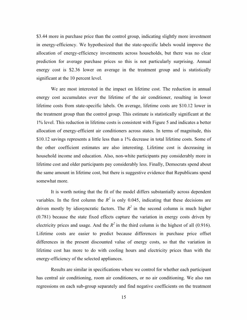
15

$3.44 more in purchase price than the control group, indicating slightly more investment

in energy-efficiency. We hypothesized that the state-specific labels would improve the

allocation of energy-efficiency investments across households, but there was no clear

prediction for average purchase prices so this is not particularly surprising. Annual

energy cost is $2.36 lower on average in the treatment group and is statistically

significant at the 10 percent level.

We are most interested in the impact on lifetime cost. The reduction in annual

energy cost accumulates over the lifetime of the air conditioner, resulting in lower

lifetime costs from state-specific labels. On average, lifetime costs are $10.12 lower in

the treatment group than the control group. This estimate is statistically significant at the

1% level. This reduction in lifetime costs is consistent with Figure 5 and indicates a better

allocation of energy-efficient air conditioners across states. In terms of magnitude, this

$10.12 savings represents a little less than a 1% decrease in total lifetime costs. Some of

the other coefficient estimates are also interesting. Lifetime cost is decreasing in

household income and education. Also, non-white participants pay considerably more in

lifetime cost and older participants pay considerably less. Finally, Democrats spend about

the same amount in lifetime cost, but there is suggestive evidence that Republicans spend

somewhat more.

It is worth noting that the fit of the model differs substantially across dependent

variables. In the first column the R2 is only 0.045, indicating that these decisions are

driven mostly by idiosyncratic factors. The R2 in the second column is much higher

(0.781) because the state fixed effects capture the variation in energy costs driven by

electricity prices and usage. And the R2 in the third column is the highest of all (0.916).

Lifetime costs are easier to predict because differences in purchase price offset

differences in the present discounted value of energy costs, so that the variation in

lifetime cost has more to do with cooling hours and electricity prices than with the

energy-efficiency of the selected appliances.

Results are similar in specifications where we control for whether each participant

has central air conditioning, room air conditioners, or no air conditioning. We also ran

regressions on each sub-group separately and find negative coefficients on the treatment

16

variable in all three regressions, but only statistically significant results for survey

participants with central air conditioners. The lower statistical significance reflects, in

part, the smaller sample sizes and that more than two-thirds of the survey participants

have central air conditioning. Finally, we also estimated regressions with interaction

effects between treatment and participant characteristics. The interaction terms are

imprecisely estimated but suggest that the gains from better labels are larger for college

graduates and democrats. See Appendix Table A1.

D. The Allocation of Energy Efficiency across Regions

Table 5 reports additional regression estimates. Focusing on cost savings across

the entire sample masks important heterogeneity. As suggested by Figure 5, participants

in low-cost states may respond differently to state-specific labels than participants in

high-cost states. The top row corresponds exactly to the regression estimates in Table 4,

but also includes estimates of lifetime cost corresponding to alternative values of the

discount rate (ρ). Estimated savings increase to $15.60 with a 6.7 percent discount rate

and fall to $7.09 with a 19.8 percent discount rate. In all cases, the savings are

statistically significant at the 5 percent level or lower.

For the regressions reported in the second through fourth rows, the sample is split

into three parts corresponding to low-, middle-, and high-energy cost states. As we saw

initially with Figure 5, the impact of state-specific labels varies considerably across

groups. Participants in low-cost states spend less upfront on air conditioners, and incur

less overall lifetime cost. With a 13.7% discount rate, lifetime savings are $6.78, a

difference that is statistically significant at the 5 percent level. Participants in medium-

cost states incur about the same amount in overall lifetime cost. For these states, state-

specific labels provide information that is very similar to the current EnergyGuide labels,

so it makes sense that there would not be large differences in behavior. Finally,

participants in high-cost states spend considerably more upfront on air conditioners, and

then incur considerably lower lifetime costs, ranging from $12.81 to $41.61 for the

discount rates we consider. In all cases the lifetime savings for this group are statistically

significant at the 5 percent level.

17

E. Aggregate Savings Nationwide from State-Specific Labels

Households can make two kinds of mistakes when buying air conditioners with

inaccurate information about operating costs. Households in low-cost states (e.g.

Massachusetts) may purchase overly energy-efficient air conditioners despite the fact

they will operate these air conditioners only a few days a year. In our experiment,

participants from low-cost states save nearly $7 on average in lifetime costs with better

information. Conversely, households in high-cost states (e.g. Florida) may purchase less

energy-efficient air conditioners than is optimal given the expected heavy usage in that

state. In our experiment, participants from high-cost states save $23 on average in

lifetime costs with better information. Overall, better information leads to private gains of

over $10 per air conditioner purchase.

Table 6 reports the aggregate national savings implied by our estimates. That is,

the table reports how much consumers would save nationwide from a shift to state-

specific EnergyGuide labels. We calculated the average lifetime cost savings across

states using a weighted average of the cost savings for low, medium, and high operating

cost states weighted by the distribution of room air conditioners in the United States as

reported in the 2009 Residential Energy Consumption Survey.20 The weighted average

lifetime cost savings is $11.60 per unit. Given nationwide annual sales of 4.4 million

units, the cost savings for room air conditioners sold in a given year is $51.0 million.21

Discounting future year savings at 13.7 percent (and assuming no increase in sales or

annual energy costs), we get a present discounted value of savings of $424 million.

Our findings suggest that state-specific labels would improve purchase decisions

not just for room air conditioners, but also for many different types of appliances. Central

air conditioners, furnaces, and heat pumps are obvious examples because cooling and

heating demand varies across states. But appliances like refrigerators, freezers, clothes 20 We used the distribution of room air conditioners rather than sales of room air conditioners due to the lack of data on the latter. 21 These calculations ignore potential responses by appliance manufacturers and retailers. In the short-run, firms might adjust pricing in response to the change in demand for different models. The U.S. appliance market has become more competitive with the recent entry of LG, Samsung, and other international manufacturers, but firms are still able to charge significant markups particularly for high-end models (Houde (2014a); Spurlock (2014)). Moreover, in the long-run manufacturers might respond to better information by changing the set of appliances offered for sale.

18

washers, and dishwashers could also benefit from state-specific labels. As we showed

earlier, residential electricity prices vary by more than 2:1 across states, so there are

significant potential efficiency gains from improved information even for products with

little predictable cross-state variation in usage.22

These estimated benefits need to be compared to the costs of implementing state-

specific labels. Requiring manufacturers to ship appliances with state-specific labels

would not require any additional appliance testing. The FTC currently maintains label

templates that manufacturers download and print. Instead of one template per appliance,

the FTC would need to maintain 50 different templates, one for each state, perhaps

accessible through a drop-down menu. At the same time it might also make sense to

automate the simple calculation required to fill in estimated yearly energy cost. Although

these changes with the FTC website would presumably be relatively inexpensive, the

more substantive administrative burden would fall on the manufacturers themselves. The

challenge for manufacturers is that labels are often attached to appliances even before it is

known where they are going to be shipped. Moreover, appliances are frequently rerouted

across states. For example, an appliance originally intended for California can end up

Nevada. It might make sense to use region-specific labels, rather than state-specific, to

reduce the amount of relabeling that is required and/or to ship appliances with labels

prepared for several different states.23

An alternative deployment option would be add a QR scan code to existing labels

which consumers could scan with their smart phones.24 The phone would then

automatically display a label with state-specific or even county-specific annual energy

22 While we have not addressed the issue of externalities associated with appliance use and the interaction with better labels, we note that carbon pricing, for example, would change – and perhaps increase – the regional variation in electricity prices. See, for example, Graff Ziven, Kotchen, and Mansur (2014). 23 The U.S. Department of Energy has taken a region-based approach with new minimum efficiency standards for central air conditioners and heat pumps. The United States has been divided into three regions (North, Southwest, and Southeast) and, beginning January 1, 2015, central air conditioners and heat pumps manufactured for the two Southern regions must meet a higher minimum efficiency standard. See U.S. Court of Appeals Case # 11-1485, April 24, 2014 for details. Interestingly, a regional standard likely decreases the potential benefits from customized labels by eliminating the least energy-efficient models in high operating cost states. 24 The new EPA vehicle mileage labels that went into effect beginning with model year 2013 include a QR scan code providing smart phone access to online information about fuel economy and environmental factors.

19

costs. This would require the FTC to maintain a website with data on average annual

energy costs that would be queried by the phone's QR scan app. The cost of including a

QR scan code on labels would be near zero, and the cost to the FTC of developing the

software and maintaining such a system would be relatively low, though whether or not

consumers would use the information is unclear. Another related deployment option

would be to develop an automated system for online retailers. By law retailers must make

EnergyGuide labels available for online shoppers and an automated system could display

labels that are tailored to each consumer’s state or county of residence. This

customization would be somewhat easier logistically than the physical labels because of

the issue of not knowing where appliances are going to be shipped.

5. Underlying Mechanisms

Having documented substantial treatment effects from the introduction of state-

specific EnergyGuide labels, we next turn to an analysis of the underlying mechanisms

driving our results. Specifically, we ask three questions: (1) Do participants understand

the labels? (2) Do participants know whether their state's annual energy cost from

operating an air conditioner is higher or lower than the national average? (3) Do

participants take local factors into account when selecting a level of efficiency?

A. Do Participants Understand the Labels?

Table 7 shows the responses to two multiple choice questions we asked

participants immediately after they made their hypothetical appliance choices. The exact

wording of the questions is provided in the table. These questions were aimed at

investigating how well participants understood the labels they had just seen. Participants

were not able to go back and look again at the labels before answering the questions.

Most participants were not able to correctly answer questions about how yearly

operating costs were calculated. Over half the participants were not sure whether the

national or state electricity price was used to compute yearly costs, and among those who

had an opinion, many incorrectly answered the question. There is no statistical difference

between the percentage of each group that thought it was the national average price (33.6

versus 30.8 percent). However, the treatment group was more likely to answer correctly

20

that it was the state price (17.0 versus 10.1 percent). This difference is statistically

significant, but indicates that only a relatively small fraction of participants in the

treatment group actually realized they were seeing operating costs calculated using state-

specific information. The responses are similar for the question about what usage level

was used. Again, over half of the participants were not sure whether national or state

information was used and again, among those who expressed an opinion there is a large

fraction of incorrect responses.

B. Do Participants Know How Their State Compares?

Part of the rationale for the current EnergyGuide labels is that individuals should

be able to “translate” the operating cost information to incorporate information about

local electricity prices and usage. The labels include the phrase, “Your cost will depend

on your utility rates and use.” And, at least in theory, an individual could transform the

estimated yearly energy cost to a more meaningful measure reflecting local information.

This hinges, however, on individuals having some sense of how their local energy prices

and usage compare to the national average.

Table 8 shows the responses to two multiple choice questions aimed at evaluating

this knowledge. We first asked participants how electricity prices in their state compare

to the national average. More than two-thirds of the participants answered that they were

not sure and, overall, only 20% of participants were able to correctly answer the question.

Participants have a somewhat better understanding of how their air conditioning usage

compares to the national average. A larger fraction of participants felt confident in taking

a position (60 percent versus 30 percent) and, overall, 40% of participants were able to

correctly answer the question.25

C. Do Participants Take Local Factors Into Account?

The evidence from the previous subsections suggests that consumers are not

going to be able to mentally adjust the information in the current EnergyGuide labels to

25 We also examined responses separately for the treatment and control groups and the distribution of responses is very similar and not statistically different (p-values 0.41 and 0.70). This suggests that participants in the treatment group are not inferring anything about their state’s electricity prices or usage based on the labels they are shown.

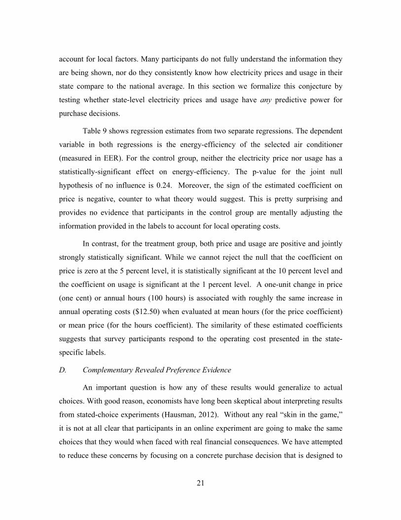
21

account for local factors. Many participants do not fully understand the information they

are being shown, nor do they consistently know how electricity prices and usage in their

state compare to the national average. In this section we formalize this conjecture by

testing whether state-level electricity prices and usage have any predictive power for

purchase decisions.

Table 9 shows regression estimates from two separate regressions. The dependent

variable in both regressions is the energy-efficiency of the selected air conditioner

(measured in EER). For the control group, neither the electricity price nor usage has a

statistically-significant effect on energy-efficiency. The p-value for the joint null

hypothesis of no influence is 0.24. Moreover, the sign of the estimated coefficient on

price is negative, counter to what theory would suggest. This is pretty surprising and

provides no evidence that participants in the control group are mentally adjusting the

information provided in the labels to account for local operating costs.

In contrast, for the treatment group, both price and usage are positive and jointly

strongly statistically significant. While we cannot reject the null that the coefficient on

price is zero at the 5 percent level, it is statistically significant at the 10 percent level and

the coefficient on usage is significant at the 1 percent level. A one-unit change in price

(one cent) or annual hours (100 hours) is associated with roughly the same increase in

annual operating costs ($12.50) when evaluated at mean hours (for the price coefficient)

or mean price (for the hours coefficient). The similarity of these estimated coefficients

suggests that survey participants respond to the operating cost presented in the state-

specific labels.

D. Complementary Revealed Preference Evidence

An important question is how any of these results would generalize to actual

choices. With good reason, economists have long been skeptical about interpreting results

from stated-choice experiments (Hausman, 2012). Without any real “skin in the game,”

it is not at all clear that participants in an online experiment are going to make the same

choices that they would when faced with real financial consequences. We have attempted

to reduce these concerns by focusing on a concrete purchase decision that is designed to

22

look similar to actual decisions that individuals face, but we recognize the limitations

inherent with stated choice, and an important priority for future research is to replicate

these experiments in the field.

In our context, it is not even possible to make strong statements about the

direction of bias. On the one hand, better labels might tend to be less effective than in the

real-world because there is no actual money at stake, so participants are going to tend to

answer these questions quickly and perhaps not read the fine print. On the other hand, our

stated-choice setting removes some additional factors like appliance manufacturer and

differences in sizes, color, and other design considerations potentially leading participants

to focus more on these labels than they would in the real-world. It is impossible to know

which of these potential biases is more important.

Federal law requires that EnergyGuide labels be displayed on all major appliances

sold in the United States. Thus, it would not be straightforward to replicate this online

experiment in the field. Strictly speaking, it would be illegal to go into an appliance

retailer and replace the current labels with labels providing state-specific information.

One possibility would be to supplement the existing labels with additional information of

some form. Although this would indeed be interesting, the results of such an experiment

would be somewhat difficult to interpret. Such a treatment would inevitably increase

attention on operating costs, and it would be difficult to disentangle the impact of that

attention from the pure information content.

Another approach to validating our stated-choice experiment is to look for

complementary evidence from actual choices. Figure 6 shows the fraction of new central

air conditioners sold in each state in 2009 that had an Energy Star rating.26 What is

potentially interesting about this figure is the lack of correlation between these choices

and the pattern of operating costs we showed in Figure 3. Operating costs are highest

throughout the South, from Texas through Louisiana, Mississippi, Alabama, Georgia,

South Carolina and Florida. So if choices are being made efficiently, we would expect to

26 We would have also been interested in examining this pattern for room air conditioners but state-level Energy Star shares are not available. These data on central air conditioners come from U.S. Department of Energy (2010) and are derived from a survey that includes about 60 percent of the retail market.

23

see large investments in energy-efficiency in these states. Instead, the states with the

highest Energy Star shares are in the Northeast and upper Midwest. The cross-state

correlation between the Energy Star share and estimated annual operating costs is -0.23.27

Thus, the correlation is actually negative, which would imply that Energy Star purchases

are biased away from what would be required for efficiency.

As always, however, it is important to interpret cross-sectional comparisons with

caution. The high penetration of Energy Star air conditioners in states like Vermont and

Massachusetts suggests that other factors including political ideology may come into play

when households make choices about energy-efficiency. Our experiment provides some

supportive evidence for this hypothesis. In particular, political party affiliation did seem

to matter for air conditioner choices in Table 4. While being affiliated with the

Democratic Party does not have a statistically significant effect, participants who are

affiliated with the Republican Party tend to choose less expensive (i.e. less energy-

efficient) air conditioners and thus spend more in annual operating cost.28 Political

ideology is not the only possible explanation for this geographic pattern of Energy Star

adoption. Air conditioning is less common in the North, so it tends to be higher-income

households making these purchases, and this compositional effect could provide an

alternative explanation.

That said, this apparent lack of positive correlation between appliance choices and

operating costs is not without precedent in the existing literature. In related work,

Jacobsen (forthcoming) finds using panel data no evidence that electricity prices increase

purchases of Energy Star appliances. Similarly, Houde (2014b) finds using transaction-

level data from a major retailer little sensitivity of appliance choices to local electricity

27 We also estimated regressions with Energy Star penetration as the dependent variable and average operating cost along with average state household income, education, gender, age, and political ideology covariates. Even after controlling for these other factors, operating cost continues to be negatively correlated with Energy Star penetration albeit with a t-statistic of -0.97. 28 Previous papers have documented similar correlations between political ideology and adoption of energy-efficient vehicles and buildings (Kahn and Vaughn, 2009). One of the potential explanations that has been suggested is that in "green" communities, driving an energy-efficient vehicle or owning an energy-efficient building could be perceived as a symbol of "status" (Kahn, 2007). We are not aware of previous attempts to correlate political ideology with air conditioner choices, but these purchases are considerably less visible than vehicles and buildings, suggesting that other more intrinsic explanations may play a role.

24

prices. These are surprising findings given how much electricity rates vary across states

but perhaps make sense given the coarse information provided by current labels and that

most consumers appear to have little understanding about how their electricity rates

compare to the national average.

Revealed preference cannot tell us how much choices would be improved by

better information, but it does provide some real-world corroboration for the evidence in

our stated-choice experiment suggesting that the current labels are not working as well as

they could. It may not be enough to simply say, as the current labels do, that “Your cost

will depend on your utility rates and use.” We may need to provide better information to

help consumers connect the dots.

E. Discussion and Implications

The state-specific labels changed participants’ behavior, so participants are not

ignoring these labels completely. But at the same time, participants are not exerting the

effort that would be required to understand the information beyond a superficial level. In

the labels the annual operating cost appears in 24-point font, bigger than all other text.

Participants in the experiment appear to have read and internalized that one number, but

then failed to read or internalize anything else. Moreover, there is no evidence of

individuals spontaneously incorporating local information when they see only national-

average information.

Most participants do not make intertemporal decisions like this regularly. Getting

a decision like this exactly right would require real time and cognitive effort, so it makes

sense that participants may try to simplify these decisions, either consciously or

unconsciously. One way to simplify the problem is to take the headline operating cost

number as given, and ignore everything else. Whether this inattention is rational or

irrational is unclear. It could be that participants are weighing the potential benefits of

becoming perfectly informed against attention and other costs and choosing consciously

to be inattentive (Sallee, 2014). Or it could be that they have unconsciously switched into

an inattentive mode and could switch back at relatively low cost.

Another point that emerges from this analysis is the distinction between

25

information programs and energy conservation programs. While providing state-specific

information to households appears to lead to more economically efficient appliance

purchases, it does not necessarily mean that aggregate energy use will fall. Additional

regression evidence in Table 10 shows that, in our experiment, electricity consumption,

in fact, does go down, by an average of 16.5 kilowatt hours per year, driven by significant

decreases in consumption high-cost states. However, this need not be the case. In general,

providing better information leads energy consumption to decrease in high-cost states but

increase in low-cost states. Whether the net change in consumption is positive or

negative depends on the type of information provided and characteristics of the

households receiving that better information. But – and this is important – better

information is efficiency enhancing regardless of the effect on energy use.29

6. Conclusion

Energy efficiency is critically important both as an element of a portfolio of

measures to reduce greenhouse gas emissions to address global climate change

(Intergovernmental Panel on Climate Change, 2014) as well as concerns about local

pollutants from the burning of fossil fuels. This paper contributes to our understanding of

the role information plays in shaping consumer purchase decisions as well as possible

instruments to improve purchase decisions for optimal levels of energy-efficient capital.

We find that better labels lead to better choices. State-specific labels decrease the

lifetime cost of air conditioning both in high- and low- operating costs states. In high-cost

states like Florida and Texas, consumers invest more in energy-efficiency and this

increase in upfront spending is outweighed by a substantial decrease in annual energy

expenditures. In low-cost states like Maine and Oregon, consumers invest less in energy-

efficiency and this decrease in upfront spending outweighs a modest increase in annual

energy expenditures.

Despite the improved allocation, there remains a puzzle. Although participants

respond to the labels, they do so without a precise understanding about how the

29 This ignores the fact that the private cost of energy may not match the social cost. For an in depth analysis of the externalities associated with energy production and consumption, see National Research Council (2009).

26

information was calculated. For example, few participants knew whether the information

they had just seen was based on state- or national-level electricity rates, even though this

information was available at the bottom of the label. One possible explanation for the

puzzle is that participants treat the label as WYSIATI. That is, when they look at the

labels they fixate on the main headline summary number in large font, while essentially

ignoring everything else. If this is correct, it has important implications for label design.

Most importantly, it suggests that we should be working hard to make sure that the

headline number is as accurate as possible, and that we should not assume that

households can “translate” information to reflect local or personal variation in prices and

usage. This conjecture suggests a fruitful line of future research, both in the lab and in

the field.

Our research has practical significance as well. The implied aggregate cost

savings for this appliance category alone exceeds $50 million annually. Moreover, our

results suggest that customized information could improve decision making not only for

air conditioners, but for many different types of appliances. While the usage of most

appliances does not vary geographically as much as air conditioning, electricity prices

vary by more than 2:1 across states, so there are potentially significant efficiency gains

from improved information even for products with little variation in usage.

27

References Allcott, Hunt. 2011a. "Consumers' Perceptions and Misperceptions of Energy Costs."

American Economic Review Papers & Proceedings no. 101 (3):98-104. Allcott, Hunt. 2011b. "Social Norms and Energy Conservation." Journal of Public

Economics no. 95 (9-10):1082-1095. Allcott, Hunt. 2013. "The Welfare Effects of Misperceived Product Costs: Data and

Calibrations from the Automobile Market." American Economic Journal: Economic Policy no. 5 (3):30-66.

Allcott, Hunt, and Todd Rogers. 2014. "The Short-Run and Long-Run Effects of

Behavioral Interventions: Experimental Evidence From Energy Conservation." American Economic Review no. 104 (10):3003-3037.

Allcott, Hunt, and Richard Sweeney. 2014. "Can Retailers Inform Consumers About

Energy Costs? Evidence from a Field Experiment." E2e Working Paper. Allcott, Hunt, and Dmitry Taubinsky. 2015. "Evaluating Behaviorally-Motivated Policy:

Experimental Evidence from the Lightbulb Market." American Economic Review no. 105 (8):2501-2538.

Allcott, Hunt, and Nathan Wozny. 2014. "Gasoline Prices, Fuel Economy, and the

Energy Paradox." Review of Economics and Statistics no. 96 (10):779-795. Ayres, Ian, Sophie Raseman, and Alice Shih. 2009. "Evidence From Two Large Field

Experiments That Peer Comparison Feedback Can Reduce Residential Energy Usage." National Bureau of Economic Research NBER Working Paper No. 15386.

Bertrand, Marianne, and Adair Morse. 2011. "Information Disclosure, Cognitive Biases,

and Payday Borrowing." Journal of Finance no. 66 (6):1865-1893. Brounen, Dirk, and Nils Kok. 2011. "On the Economics of Energy Labels in the Housing

Market." Journal of Environmental Economics and Management no. 62 (2):166-179.

Busse, Megan R., Christopher R. Knittel, and Florian Zettelmeyer. 2013. "Are

Consumers Myopic? Evidence from New and Used Car Purchases." American Economic Review no. 103 (1):220-256.

Camilleri, Adrian R., and Richard P. Larrick. 2014. "Metric and Scale Design as Choice

Architecture Tools." Journal of Public Policy and Marketing no. 33 (1):108-125.

28

Collaborative Labeling and Appliance Standards Program (CLASP). 2014. Global S&L Database. CLASP 2014 [cited Sept. 25, 2014 2014]. Available from http://www.clasponline.org/en/Tools/Tools/SL_Search.aspx.

Davis, Lucas W. 2008. "Durable Goods and Residential Demand for Energy and Water:

Evidence from a Field Trial." RAND Journal of Economics no. 39 (2):530-546. Dubin, Jeffrey A., and Daniel L. McFadden. 1984. "An Econometric Analysis of

Residential Electric Appliance Holdings and Consumption." Econometrica no. 52 (2):345-362.

Federal Trade Commission. 2014. EnergyGuide Labeling: FAQs for Appliance

Manufacturers 2014 [cited October 9, 2014 2014]. Available from http://www.business.ftc.gov/documents/bus-82-energyguide-labels-faqs.

GfK. KnowledgePanel Design Summary 2013 [cited September 26, 2014. Available

from http://www.gfk.com/Documents/GfK-KnowledgePanel-Design-Summary.pdf.

GfK. nd. "GfK Methodology." Gillingham, Kenneth, Richard G. Newell, and Karen Palmer. 2009. "Energy Efficiency

Economics and Policy." Annual Review of Resource Economics no. 1 (1):597-619.

Gillingham, Kenneth, and Karen Palmer. 2014. "Bridging the Energy Efficiency Gap:

Policy Insights from Economic Theory and Empirical Evidence." Review of Environmental Economics and Policy no. 8 (1):18-38.

Graff Ziven, Joshua, Matthew J. Kotchen, and Erin T. Mansur. 2014. "Spatial and

Temporal Heterogeneity of Marginal Emissions: Implications for Electric Cars and Other Electricity-Shifting Policies." Journal of Economic Behavior and Organization no. 107 (Part A, November):248-268.

Hastings, Justine S., and Jeffrey M. Weinstein. 2008. "Information, School Choice, and

Academic Achievement: Evidence From Two Experiments." Quarterly Journal of Economics no. 123 (4):1373-1414.

Hausman, Jerry A. 1979. "Individual Discount Rates and the Purchase and Utilization of

Energy-Using Durables." Bell Journal of Economics no. 10 (1):33-54. Hausman, Jerry A. 2012. "Contingent Valuation: From Dubious to Hopeless." Journal of

Economic Perspectives no. 26 (4):43-56. Houde, Sebastien. 2014a. "Bunching with the Stars: How Firms Respond to

Environmental Certification."

29

Houde, Sebastien. 2014b. "How Consumers Respond to Environmental Certification and

the Value of Energy Information." E2e Project Working Paper 007. Hoxby, Caroline, and Sarah Turner. 2013. "Expanding College Opportunities for High-

Achieving, Low Income Students." SIEPR Discussion Paper Intergovernmental Panel on Climate Change. 2014. Climate Change 2014: Mitigation of

Climate Change, Working Group III Contribution to the Fifth Assessment Report of the Intergovernmental Panel on Climate Change.

Jacobsen, Grant. forthcoming. "Do Energy Prices Influence Investment in Energy

Efficiency? Evidence from Energy Star Appliances." Journal of Environmental Economics and Management.

Kahn, Matthew E. 2007. "Do Greens Drive Hummers? Environmental Ideology as a

Determinant of Consumer Choice." Journal of Environmental Economics and Management no. 54:129-145.

Kahn, Matthew E., and Ryan K. Vaughn. 2009. "Green Market Geography: The Spatial

Clustering of Hybrid Vehicles and LEED Registered Buildings." B.E. Journal of Economic Analysis & Policy no. 9 (2, Article 2):1-24.

Kahneman, Daniel. 2011. Thinking Fast and Slow. New York: Farrar, Strauss and

Giroux. Kling, Jeffrey R., Sendhil Mullainathan, Eldar Shafir, Lee C. Vermeulen, and Marian V.

Wrobel. 2012. "Comparison Friction: Experimental Evidence from Medicare Drug Plans." Quarterly Journal of Economics no. 127 (1):199-235.

Metcalf, Gilbert E. 1994. "Economics and Rational Conservation Policy." Energy Policy

no. 22 (10):819-825. Metcalf, Gilbert E., and Kevin A. Hassett. 1999. "Measuring the Energy Savings From

Home Improvement Investments: Evidence From Monthly Billing Data." Review of Economics and Statistics no. 81 (3):516-528.

National Research Council. 2009. Hidden Costs of Energy: Unpriced Consequences of

Energy Production and Use. Washington, DC: National Academies Press. Newell, Richard G., and Juha V. Siikamaki. 2014. "Nudging Energy Efficiency Behavior:

The Role of Information Labels." Journal of the Association of Environmental and Natural Resource Economists no. 1 (4):555-598.

30

Newell, Richard G., and Juha V. Siikamaki. 2015. "Individual Time Preferences and Energy Efficiency." American Economic Review: Papers & Proceedings no. 105 (5):196-200.

Revelt, David, and Kenneth Train. 1998. "Mixed Logit with Repeated Choices:

Households' Choices of Appliance Efficiency Level." Review of Economics and Statistics no. 80 (4):647-657.

Sallee, James M. 2014. "Rational Inattention and Energy Efficiency." Journal of Law and

Economics no. 57 (3):781-820. Spurlock, Anna. 2014. "Appliance Efficiency Standards and Price Discrimination."

Lawrence Berkeley Lab Thorne, Jennifer, and Christine Egan. 2002. "An Evaluation of the Federal Trade

Commission's EnergyGuide Appliance Label." American Council for an Energy Efficient Economy

U.S. Department of Energy. 2014. Residential Energy Consumption Survey (RECS) 2009.

DOE EIA 2009 [cited September 25, 2014 2014]. Available from http://www.eia.gov/consumption/residential/data/2009/.

U.S. Department of Energy. 2009 Unit Shipment Data Collection Forms. Energy Star

2010. Available from https://www.energystar.gov/index.cfm?c=partners.unit_shipment_data_archives.

U.S. Department of Energy. 2013a. Electric Power Annual. Washington, DC:

Government Printing Office. U.S. Department of Energy. 2014. Energy Star Unit Shipment and Market Penetration

Report Calendar Year 2012 Summary. DOE 2013b [cited September 25, 2014 2014]. Available from https://www.energystar.gov/index.cfm?c=partners.unit_shipment_data_archives.

U.S. Department of Energy. 2014. Room Air Conditioner Savings Calculator 2014 [cited

September 26, 2014 2014]. Available from http://www.energystar.gov/buildings/sites/default/uploads/files/RoomAC_Calculator.xls.

U.S. Energy Information Administration. 2014a. Annual Energy Outlook 2014.

Washington, DC. U.S. Energy Information Administration. 2014b. Assumptions to the Annual Energy

Outlook 2014: Residential Demand Model. Washington, DC: U.S. Department of Energy.

31

Wiel, Stephen, and James E. McMahon. 2001. Energy-Efficiency Labels and Standards. Washington, DC: Collaborative Labeling and Appliance Standards Program (CLASP).

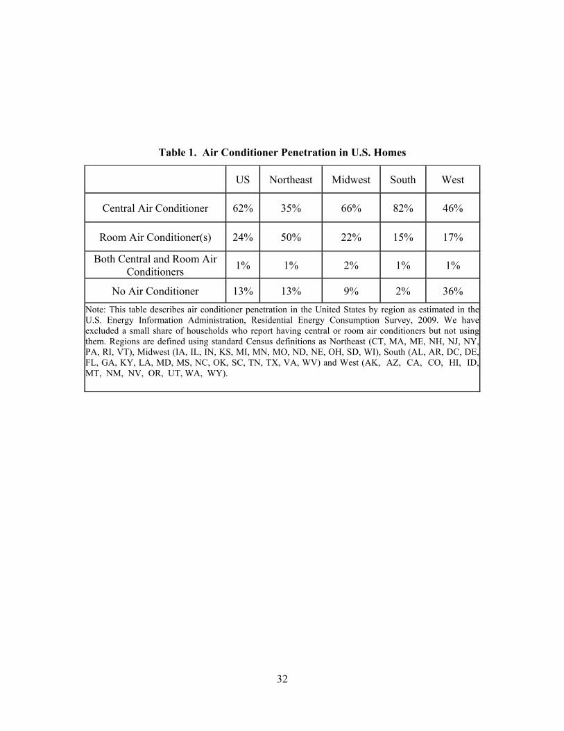
32

Table 1. Air Conditioner Penetration in U.S. Homes

US Northeast Midwest South West

Central Air Conditioner 62% 35% 66% 82% 46%

Room Air Conditioner(s) 24% 50% 22% 15% 17%

Both Central and Room Air Conditioners 1% 1% 2% 1% 1%

No Air Conditioner 13% 13% 9% 2% 36% Note: This table describes air conditioner penetration in the United States by region as estimated in the U.S. Energy Information Administration, Residential Energy Consumption Survey, 2009. We have excluded a small share of households who report having central or room air conditioners but not using them. Regions are defined using standard Census definitions as Northeast (CT, MA, ME, NH, NJ, NY, PA, RI, VT), Midwest (IA, IL, IN, KS, MI, MN, MO, ND, NE, OH, SD, WI), South (AL, AR, DC, DE, FL, GA, KY, LA, MD, MS, NC, OK, SC, TN, TX, VA, WV) and West (AK, AZ, CA, CO, HI, ID, MT, NM, NV, OR, UT, WA, WY).

33

Table 2. Testing for Balance in Randomized Sample Control Treatment p-value

(1) (2) (3) Annual Household Income (in dollars) 72,817 70,848 0.363

High School Graduate 0.874 0.874 1.000 College Graduate 0.289 0.289 1.000 Household Size 2.745 2.756 0.871 Married 0.533 0.533 0.981 Employed 0.582 0.564 0.408 Age 65 and older 0.174 0.179 0.723 Female 0.519 0.519 1.000 Nonwhite 0.338 0.338 1.000 Homeowner 0.728 0.695 0.100 Multiunit Property 0.250 0.256 0.718 Household has a Central Air Conditioner 0.655 0.675 0.322

Democratic Affiliation 0.316 0.314 0.942 Republican Affiliation 0.217 0.244 0.115 Average Residential Electricity Price in the State of Residence (cents per kWh)

12.49 12.32 0.088

Average Annual Hours of Air Conditioning Use in the State of Residence

1,260 1,265 0.840

Annual Cost of Operating a Medium-Sized Room Air Conditioner in the State of Residence (in dollars)

154.58 153.04 0.601

Note: This table tests for balance between the control and treatment groups. There are 1231 participants in the control group and 1209 participants in the treatment group. Columns 1 and 2 report means of the variables listed in the row headings, weighted using sampling weights. Proportion high school graduate, college graduate, employment status, and the other individual characteristics correspond to the individual in each household who participates in the KnowledgePanel, not for the head of household. The annual cost of operating a medium-sized room air conditioner is calculated for a 10,000 Btu unit with an EER of 10.0. Column 3 reports p-values from tests that the weighted means in the two groups are equal.

34

Table 3. Conditional Logit Regression Results

Variable Coefficient Estimate

Purchase Price (PP) -0.00223 (0.0004)

Energy cost (EC) -0.01281 (0.0016)

Ratio of the Coefficient Estimates on PP and EC

0.174 (0.013)

Implied Discount Rate ( ) 0.137 (0.017)

Note: This table reports coefficients from a conditional logit model estimated using all 7,275 choices made by the 2,440 participants in our online experiment. There are slightly less than 3 choices per participant because a small number of participants failed to finish the experiment. The implied discount rate is calculated using an assumed 12-year appliance lifetime. Observations are weighted using sampling weights. Standard errors, clustered by state, are reported in parentheses. For the ratio we calculate the standard error using the delta method and for the implied discount rate we calculate the standard error using bootstrap with 1000 replications. All coefficient estimates are statistically significant at the 1 percent level.

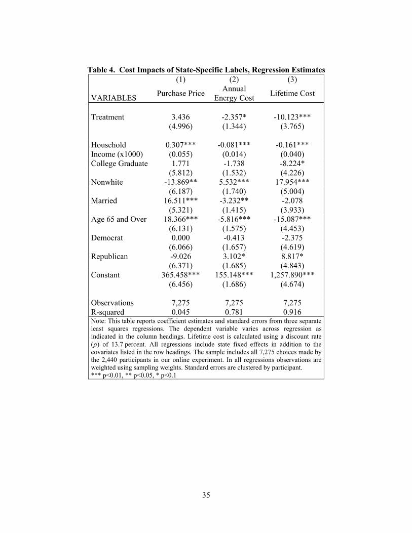
35

Table 4. Cost Impacts of State-Specific Labels, Regression Estimates (1) (2) (3)

VARIABLES Purchase Price Annual Energy Cost Lifetime Cost

Treatment 3.436 -2.357* -10.123***

(4.996) (1.344) (3.765) Household Income (x1000)

0.307*** -0.081*** -0.161*** (0.055) (0.014) (0.040)

College Graduate 1.771 -1.738 -8.224* (5.812) (1.532) (4.226)

Nonwhite -13.869** 5.532*** 17.954*** (6.187) (1.740) (5.004)

Married 16.511*** -3.232** -2.078 (5.321) (1.415) (3.933)

Age 65 and Over 18.366*** -5.816*** -15.087*** (6.131) (1.575) (4.453)

Democrat 0.000 -0.413 -2.375 (6.066) (1.657) (4.619)

Republican -9.026 3.102* 8.817* (6.371) (1.685) (4.843)

Constant 365.458*** 155.148*** 1,257.890*** (6.456) (1.686) (4.674)

Observations 7,275 7,275 7,275 R-squared 0.045 0.781 0.916 Note: This table reports coefficient estimates and standard errors from three separate least squares regressions. The dependent variable varies across regression as indicated in the column headings. Lifetime cost is calculated using a discount rate ( ) of 13.7 percent. All regressions include state fixed effects in addition to the covariates listed in the row headings. The sample includes all 7,275 choices made by the 2,440 participants in our online experiment. In all regressions observations are weighted using sampling weights. Standard errors are clustered by participant. *** p<0.01, ** p<0.05, * p<0.1

36

Table 5. Cost Impacts of State-Specific Labels, Additional Regression Estimates Lifetime Cost

Purchase Price Annual Energy Cost =.137 =.067 =.198

(1) (2) (3) (4) (5) Entire Sample $3.44

(5.00) -$2.36* (1.34)

-$10.12*** (3.76)

-$15.60** (6.61)

-$7.09*** (2.49)

Low Operating Cost States -$12.49 (7.82)

$0.99 (1.09)

-$6.78** (2.77)

-$4.48 (2.87)

-$8.06** (3.58)

Medium Operating Cost States

$1.50 (9.35)

-$0.02 (2.31)

$1.37 (4.40)

$1.32 (9.58)

$1.40 (1.99)

High Operating Cost States $22.86** (9.02)

-$7.98** (3.23)

-$23.06** (9.98)

-$41.61** (17.39)

-$12.81** (5.97)

Note: This table reports coefficient estimates and standard errors corresponding to the treatment indicator variable from twenty separate least squares regressions. Positive numbers indicate a higher price or cost for the treatment group. The dependent variable varies across regressions as indicated in the column headings. Lifetime costs are calculated using the discount rates as indicated. All regressions include state fixed effects as well as household income and indicator variables for college graduate, non-white, married, age 65 or over, and political party affiliation. For the first row the sample includes all 7,275 choices made by the 2,440 participants in our online experiment. For the regressions reported in the second through fourth rows, states are divided into three groups (terciles) based on average energy costs (residential electricity prices multiplied by annual hours of air conditioning use) and then regressions are run using participants from each subset of states. In all regressions observations are weighted using sampling weights. Standard errors are clustered by participant. *** p<0.01, ** p<0.05, * p<0.1

37

Table 6. Implied Aggregate National Savings from State-Specific Labels Lifetime Cost Savings per Room Air Conditioner (weighting by RAC distribution across states)

$11.60

Annual U.S. Sales of Room Air Conditioners 4.4 million Total Cost Savings per Year $51.0 million Total Cost Savings – All Future Years (discounted at 13.7 percent) $423.5 million Note: This table reports the implied aggregate national savings implied by our estimates. Lifetime cost savings per air conditioner come from the full-sample regression estimate corresponding to a discount rate of 13.7%. Annual sales of room air conditioners come from U.S. Department of Energy (2013b). Total cost savings for all room air conditioners is the product of the first and second rows. The final row reports the present discounted value of total cost savings implied by a permanent switch to state-specific labels.

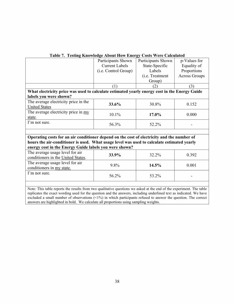
38

Table 7. Testing Knowledge About How Energy Costs Were Calculated Participants Shown

Current Labels (i.e. Control Group)

Participants Shown State-Specific

Labels (i.e. Treatment

Group)

p-Values for Equality of Proportions

Across Groups

(1) (2) (3) What electricity price was used to calculate estimated yearly energy cost in the Energy Guide labels you were shown? The average electricity price in the United States 33.6% 30.8% 0.152

The average electricity price in my state. 10.1% 17.0% 0.000

I’m not sure. 56.3% 52.2% -

Operating costs for an air conditioner depend on the cost of electricity and the number of hours the air-conditioner is used. What usage level was used to calculate estimated yearly energy cost in the Energy Guide labels you were shown?The average usage level for air conditioners in the United States. 33.9% 32.2% 0.392

The average usage level for air conditioners in my state. 9.8% 14.5% 0.001

I’m not sure. 56.2% 53.2% -

Note: This table reports the results from two qualitative questions we asked at the end of the experiment. The table replicates the exact wording used for the question and the answers, including underlined text as indicated. We have excluded a small number of observations (<1%) in which participants refused to answer the question. The correct answers are highlighted in bold. We calculate all proportions using sampling weights.

39

Table 8: Testing Knowledge About How State Energy Costs Compare to National Average

The national average residential electricity price is 12.4 cents per kilowatt hour (kWh). How does the average residential electricity price in your state compare to the national average? My state’s electricity prices are higher than the national average. 14.3%

My state’s electricity prices are lower than the national average. 16.6%

I’m not sure. 69.2%

Percentage Correct 20.2%

How do you think average air conditioning usage in your state compares to the average usage nationally? Average usage in my state is probably higher than the national average. 30.6%

Average usage in my state is probably lower than the national average. 28.1%

I’m not sure. 41.3%

Percentage Correct 40.4%

Note: This table reports the results from two questions we asked at the end of the experiment. The table replicates the exact wording used for the question and the answers, including underlined text as indicated. We have excluded a small number of observations (<1%) in which participants refused to answer the question. The percentage correct is the fraction of participants who are able to answer the question (i.e. they don’t respond “I’m not sure”) and are correct in how their local conditions compare to the national average. We calculate all proportions using sampling weights.

40

Table 9. Do Participants Take Local Factors Into Account? Participants Shown

Current Labels (i.e. Control Group)

Participants Shown State-Specific Labels

(i.e. Treatment Group) (1) (2) Electricity Price (cents per

kWh) -0.036 (0.025)

0.041* (0.024)

Annual Hours of Air Conditioning Usage

(in 100s)

0.005 (0.008)

0.040*** (0.008)

p-value for joint test that price and usage do not influence EER choice

0.24 0.00

Number of Observations 3670 3605 Note: This table reports estimated coefficients and standard errors from two separate regressions. For column (1) the sample is restricted to the 3,670 choices made by participants in the control group and for column (2) the sample is restricted to the 3,605 choices made by participants in the treatment group. The dependent variable in both regressions is the energy-efficiency of the selected air conditioner (measured in EER). In addition to the independent variables listed in the row headings, both regressions include household income and indicator variables for college graduate, non-white, married, age 65 or over, and political party affiliation. In both regressions observations are weighted using sampling weights. Standard errors are clustered by participant. *** p<0.01, ** p<0.05, * p<0.1

41

Table 10. The Impact of State-Specific Labels on Electricity Consumption

Annual Electricity Consumption

(in kilowatt hours) Entire Sample -16.5

(11.1) Low Operating Cost States 10.2

(9.2) Medium Operating Cost States 8.5

(16.2) High Operating Cost States -64.6**

(27.0) Note: This table reports coefficient estimates and standard errors corresponding to the treatment indicator variable from four separate least squares regressions. The dependent variable in all regressions is the annual electricity consumption in kilowatt hours of the air conditioner selected by the participant based on annual cooling hours in the state where the participant lives. All regressions include state fixed effects as well as household income and indicator variables for college graduate, non-white, married, age 65 or over, and political party affiliation. For the first row the sample includes all 7,275 choices made by the 2,440 participants in our online experiment. For the regressions reported in the second through fourth rows, states are divided into three groups (terciles) based on average energy costs (residential electricity prices multiplied by annual hours of air conditioning use) and then regressions are run using participants from each subset of states. In all regressions observations are weighted using sampling weights. Standard errors are clustered by participant. *** p<0.01, ** p<0.05, * p<0.1

42

Figure 1: Annual Cooling Hours by State

0 − 500500 − 10001000 − 15001500 − 20002000 − 25002500 − 3000

43

Figure 2: Residential Electricity Prices by State

8 − 1010 − 1212 − 1414 − 1616 − 18

Cents/kWh

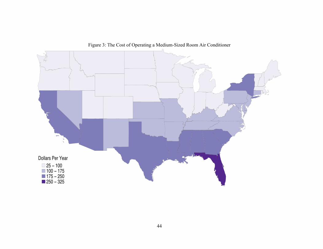
44

Figure 3: The Cost of Operating a Medium-Sized Room Air Conditioner

25 − 100100 − 175175 − 250250 − 325

Dollars Per Year

45

Figure 4: Control and Treatment Labels

Control Group Treatment Group

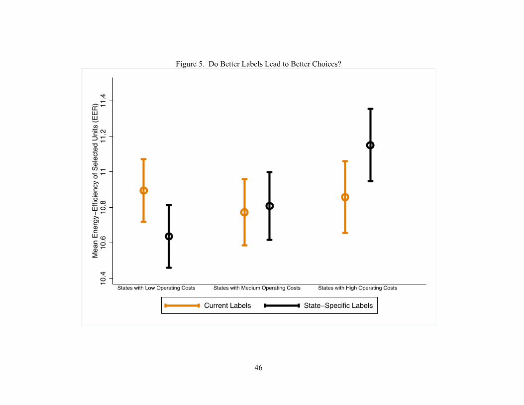
46

Figure 5. Do Better Labels Lead to Better Choices?

10.4

10.6

10.8

1111

.211

.4M

ean

Ener

gy−E

ffici

ency

of S

elec

ted

Uni

ts (E

ER)

States with Low Operating Costs States with Medium Operating Costs States with High Operating Costs

Current Labels State−Specific Labels

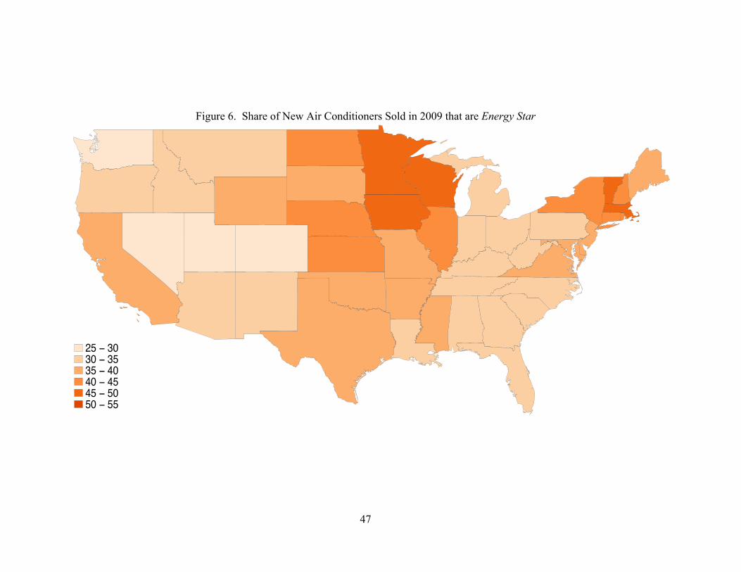
47

Figure 6. Share of New Air Conditioners Sold in 2009 that are Energy Star

25 − 3030 − 3535 − 4040 − 4545 − 5050 − 55

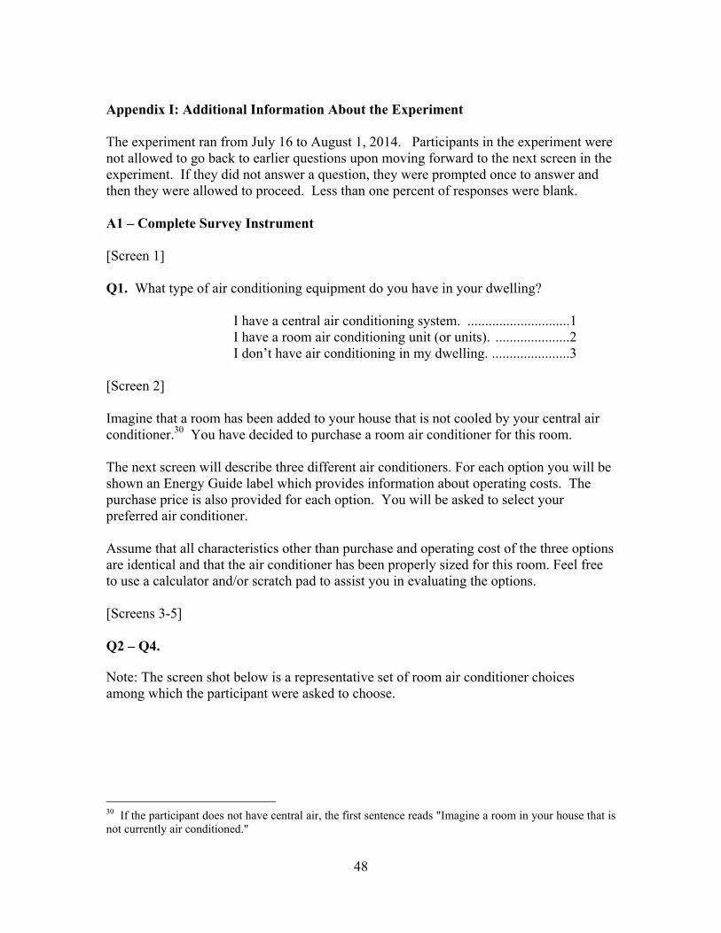
48

Appendix I: Additional Information About the Experiment The experiment ran from July 16 to August 1, 2014. Participants in the experiment were not allowed to go back to earlier questions upon moving forward to the next screen in the experiment. If they did not answer a question, they were prompted once to answer and then they were allowed to proceed. Less than one percent of responses were blank. A1 – Complete Survey Instrument [Screen 1] Q1. What type of air conditioning equipment do you have in your dwelling?

I have a central air conditioning system. .............................1 I have a room air conditioning unit (or units). .....................2 I don’t have air conditioning in my dwelling. ......................3

[Screen 2] Imagine that a room has been added to your house that is not cooled by your central air conditioner.30 You have decided to purchase a room air conditioner for this room. The next screen will describe three different air conditioners. For each option you will be shown an Energy Guide label which provides information about operating costs. The purchase price is also provided for each option. You will be asked to select your preferred air conditioner. Assume that all characteristics other than purchase and operating cost of the three options are identical and that the air conditioner has been properly sized for this room. Feel free to use a calculator and/or scratch pad to assist you in evaluating the options. [Screens 3-5] Q2 – Q4. Note: The screen shot below is a representative set of room air conditioner choices among which the participant were asked to choose.

30 If the participant does not have central air, the first sentence reads "Imagine a room in your house that is not currently air conditioned."

49

[Screen 6] Q5. What electricity price was used to calculate estimated yearly energy cost in the Energy Guide labels you were shown?

The average electricity price in the United States. ...........................................................1

The average electricity price in my state. .........2 I’m not sure. .....................................................3

[Screen 7] Q6. The national average residential electricity price is 12.4 cents per kilowatt hour (kWh). How does the average residential electricity price in your state compare to the national average?

My state’s electricity prices are higher than the national average. ..........................................1

My state’s electricity prices are lower than the national average. ..........................................2

I’m not sure. .....................................................3 [Screen 8] Q7. Operating costs for an air conditioner depend on the cost of electricity and the number of hours the air-conditioner is used. What usage level was used to calculate estimated yearly energy cost in the Energy Guide labels you were shown?

The average usage level for air conditioners in the United States. .........................................1

50

The average usage level for air conditioners in my state. .......................................................2

I’m not sure. .....................................................3 [Screen 9] Q8. How do you think average air conditioning usage in your state compares to the average usage nationally?

Average usage in my state is probably higher than the national average. .............................1

Average usage in my state is probably lower than the national average. ............................2

I’m not sure. .....................................................3 [Screen 10] Q9. How do you think air conditioning usage in your home compares to the average usage in your state?

Usage in my home is probably higher than the state average. ................................................1

Usage in my home is probably lower than the state average. ................................................2

Usage in my home is probably very close to the state average. ................................................3

End of Experiment

A2 –Sampling Design 1. Sample designed to match key benchmarks

• Gender: Male or Female • Age: 18–29, 30–44, 45–59, and 60+ • Race/Ethnicity: Hispanic and non-Hispanic White, Black, Other, and 2+ Races • Education: Less than High School, High School, Some College, Bachelor and

beyond • Census Region: Northeast, Midwest, South, and West • Household Income: $0-$10K, $10K-<$25K, $25K-<$50K, $50K-<$75K, $75K-

<$100K, and $100K+ • Home Ownership: Own or Rent/Other • Metropolitan Area: Yes or No • Home Internet Access: Yes or No

2. Study specific final weights computed to adjust for experiment-specific nonresponse

along the following dimensions x gender x race/ethnicity

51

x education x census region x household income x home internet service

A3 – Appliance Choice Questions Each participant in the experiment was shown a screen with three room air conditioner choices and asked to select their most preferred model. The choices ranged from least to most expensive. More energy-efficient air conditioners were more expensive. After selecting their preferred model, they were asked to make two additional purchase decisions in an identical manner to their first selection decision. The design matrix for the three sets of choices was as follows:

Table A1. Purchase Prices for Air Conditioner Choices Energy Efficiency Rating (EER) 7.8 11.0 13.1

Decision 1 $200 $420 $550 Decision 2 $200 $505 $600 Decision 3 $200 $335 $440

That is, the energy-efficiency rating of the three choices was the same for all participants and all decisions. We varied the purchase prices across decisions as indicated above. For all three questions, participants were shown labels that calculated energy costs as a function of the EER rating (7.8, 11.0, or 13.1) and either average national usage and electricity prices (control group) or average state usage and electricity prices. Annual energy costs (EC) are given by the following formula:

(A1) ∙

where BTU is the rated size of the air conditioner (10,000 BTU's for our experiment).

We designed the choice set for our experiment to match the range of EER values available for 10,000 BTU room air conditioners for sale in the United States in 2014. Then we selected the purchase prices based on simulation evidence to maximize the precision of our estimates. In particular, we selected the combination of choice sets which in ex ante simulations minimized the standard error on the ratio of the coefficient estimates on purchase price and energy cost. For these simulations, we constructed synthetic nationally-representative data based on an assumed distribution for the ratio of the coefficients on purchase price and energy cost. For each observation we simulated choices using draws from an extreme value distribution. We included both a treatment group and a control group and assumed both would take the information in the labels at face value. Then with the generated “data” we estimated the ratio of the coefficient

52

estimates on purchase price and energy cost and examined the distribution of choices across states as in Figure 5 from the paper. The choice sets described above were those that minimized the standard error of the estimated ratio and provided a good mix of choices across states for both the treatment and control groups.

53

Appendix II: Additional Results

Table A1. Cost Impacts of State-Specific Labels, Additional Results with Interaction Terms

(1) (2) (3)

VARIABLES Purchase Price Annual Energy Cost Lifetime Cost

Treatment -7.95 0.771 -3.52

(9.47) (2.56) (7.25) Treatment x Household income (1000s)

0.054 (0.103)

-.004 (.027)

.030 (.076)

Treatment x College Graduate

13.3 (11.6)

-5.10* (3.04)

-16.0* (8.39)

Treatment x Democrat

11.7 (10.9)

-4.33 (2.96)

-13.2 (8.29)

Household Income ($1000s)

0.285*** -0.080*** -0.176*** (0.076) (0.021) (0.060)

College Graduate -5.07 0.884 0.006 (8.51) (2.27) (6.25)

Nonwhite -13.85** 5.56*** 18.1*** (6.18) (1.74) (4.99)

Married 16.3*** -3.17** -1.97 (5.32) (1.41) (3.91)

Age 65 and Over 18.6*** -5.88*** -15.2*** (6.14) (1.57) (4.43)

Democrat -5.92 1.77 4.27 (8.24) (2.23) (6.09)

Republican -8.83 3.04* 8.66* (6.37) (1.68) (4.83)

Constant 371*** 153*** 1,254*** (7.59) (1.99) (5.60)

Observations 7,275 7,275 7,275 R-squared 0.046 0.781 0.916 Note: This table is identical to Table 4 in the paper except we have added interaction terms for household income, college graduate, and Democrat. *** p<0.01, ** p<0.05, * p<0.1