Beta Is Still Alive!∗

Yexiao Xuand

Yihua Zhao

School of ManagementThe University of Texas at Dallas

This revision: March 2012

Abstract

This paper investigates whether beta can predict the expected return after control-ling for the beta instability resulting from shift in the covariance structure. Such a shift isdriven by idiosyncratic volatility’s clientele effect: speculative investors prefer stocks withhigh idiosyncratic volatility. Consequently, these stocks tend to have low future returnsfrom overpricing, and high beta because clientele-based trading also contains systematiccomponent. Indeed, we find that the beta estimate of the current period is positivelyrelated to the beta estimate and negatively related to the idiosyncratic volatility measureof the last period. More important, different from existing studies, we find that betaestimates of the current period can significantly explain the cross-sectional differences infuture returns of individual stocks, when allowing for an interaction between the currentidiosyncratic volatility and the beta estimates. We also show that our simple model canpredict the historical expected return well. All results are robust with respect to differentmeasures of beta and idiosyncratic volatility and to different subsamples.

Key Words: Expected Return, Idiosyncratic Volatility, Beta Instability, and Misspric-ing

∗We are indebt to John Y. Campbell, Michael Rebello, Harold Zhang, Feng Zhao for his insightful comments.We have also benefited from helpful comments from seminar participants at Cheung Kong Graduate School ofBusiness and the University of Texas at Dallas. The corresponding author’s address is: Yexiao Xu, 800 WestCampbell Road, SM31, The University of Texas at Dallas, Richardson, TX 75083; Telephone (972)883-6703;FAX (972)883-6522; Email: yexiaoxu@utdallas.edu.

i

Beta Is Still Alive!

Abstract

This paper investigates whether beta can predict the expected return after control-ling for the beta instability resulting from shift in the covariance structure. Such a shift isdriven by idiosyncratic volatility’s clientele effect: speculative investors prefer stocks withhigh idiosyncratic volatility. Consequently, these stocks tend to have low future returnsfrom overpricing, and high beta because clientele-based trading also contains systematiccomponent. Indeed, we find that the beta estimate of the current period is positivelyrelated to the beta estimate and negatively related to the idiosyncratic volatility measureof the last period. More important, different from existing studies, we find that betaestimates of the current period can significantly explain the cross-sectional differences infuture returns of individual stocks, when allowing for an interaction between the currentidiosyncratic volatility and the beta estimates. We also show that our simple model canpredict the historical expected return well. All results are robust with respect to differentmeasures of beta and idiosyncratic volatility and to different subsamples.

Key Words: Expected Return, Idiosyncratic Volatility, Beta Instability, and Misspricing

ii

1 Introduction

The Capital asset pricing model (CAPM) of Sharpe (1964), Lintner (1965), and Black (1972)

predicts that differences in the expected returns of individual securities are completely deter-

mined by the covariance based beta measure of risk. Many empirical studies including Fama

and French (1992), however, provide no or weak evidence to support this prediction. In this

study, we show that the lack of empirical evidence is largely due to short-run shifts in the co-

variance structure between individual stock return and the market return. We further identify

that such a shift can be predicted by idiosyncratic volatility. Consequently, we provide strong

evidence in supporting a positive relation between the beta measure of risk and the expected

return once controlling for the interaction between beta and idiosyncratic volatility.

Although the classical CAPM model is an equilibrium model, it is static in nature with

a constant beta measure of risk for each security. There are several reasons, however, to

believe that the covariance based beta measure of risk might shift in structure over time.

Perhaps, Merton (1973) is the first one to propose a model that allows for time-varying risk as

a result of changes in the investment opportunities. Using labor income as a proxy for time-

varying investment opportunities, Jagannathan and Wang (1996) provide evidence on the

validity of the conditional CAPM.1 Alternatively, one can treat the position held by equity-

holders as a call option on the firm’s total asset (Black and Scholes, 1973) since they have the

limited liability and the residual claim. Following the idea, Galai and Masulis (1976) (also

see Berk, Green, and Naik, 1999) have shown that the equity beta will vary not only with

leverage, but also with the volatility of underlying assets even when the asset beta is stable.

Bernardo, Chowdhry, and Goyal (2007) and Da, Guo, and Jagannathan (2011) have provide

some empirical evidence in supporting this view.1Lewellen and Nagel (2006) find that the covariance between time-varying beta and time-varying risk pre-

mium is too small to explain deviations from the CAPM.

1

In this paper, we propose and test an alternative explanation for the failure of the beta

measure of risk to differentiate the cross-sectional return differences of individual securities.

Using daily returns within a month to estimate a monthly beta measure of an individual stock,

we find that the current and the next month beta estimates are weakly correlated and vary

a lot (with an average autocorrelation being less than 25%). This means that even when the

CAPM holds month by month, it is difficult to use the past beta measure to predict next month

returns. Such a large instability in the beta measure is unlikely to be a result of changing

fundamental risks of a firm which tend to occur over a longer period. Estimation errors are also

implausible to account for such large changes in the beta measure since betas are estimated

using high frequency returns. One possible explanation is the speculative investment behavior

of both institutions and individual investors who tend to chase certain stocks. As a result,

not only these stocks tend to be over- or under-priced relative to their rational prices, but

the collective activities of these investors will also move the market in the same direction as

well. Therefore, the current beta estimates of these stocks will rise temporarily. Moreover,

if over-pricing reverses with a lag because of short-sale constraints, returns tend to drop in

the subsequent periods. Such a negative relation between current beta and future returns will

obscure the true CAPM relation.

There are ample evidence to support our view. Using mutual fund equity holdings data,

Falkenstein (1996) shows that mutual funds have a significant preference towards stocks with

high visibility and are averse to stocks with low idiosyncratic volatility. Based on the Japanese

experience from 1975 to 2003, Chang and Dong (2006) find that institutional herding is

positively related to idiosyncratic volatility. For individual investors, Han and Kumar (2008)

have shown that retail investors prefer to hold and actively trade high idiosyncratic volatility

stocks due to their propensity to speculate. Such special preference by investors’ will not only

move the prices of these individual stocks but will move the market as well. Using both the

2

TAQ and ISSM data, Barber, Odean, and Zhu (2009) show that not only individual investors’

trading tends to be correlated, but their coordinated trading move the market in a substantial

way that causes significant future return difference between heavily bought and heavily sold

stocks. One thing in common from all these studies is investors’ preference toward stocks with

high idiosyncratic volatility. If this is the case, the possible instability of the beta measure

should be related to idiosyncratic volatility. Following this logic, idiosyncratic volatility can

predict changes in beta estimates, which means we might be able to restore the CAPM relation

once controlling for the instability issue.

Indeed, for stocks with large betas and high idiosyncratic volatilities in the current month,

future betas tend to be low. At the same time, these stocks also appear to have low future

returns due to limited arbitrage (see, Ang, et. al., 1996). In other words, contemporaneously,

the CAPM relation seems to hold because small (large) beta seems to be associated with low

(high) return. However, the predictive cross-sectional regression will fail. After controlling for

the interactive effect between beta and idiosyncratic volatility, we show that the rolling beta

measure estimated based on the past monthly returns (see Fama and French, 1992) can explain

the cross-sectional return differences of individual stocks. Moreover, if it is these stocks with

high current betas and large idiosyncratic volatilities but low future returns that obscure the

true beta and return relation, we should expect to see that the CAPM relation holds for the

rest of the stocks. After deleting 10% of the stocks with the largest beta and idiosyncratic

volatility (accounting for 5% of the market capitalization), the 25 size and book-to-market

sorted portfolio returns using the remaining stocks are significantly and positively related to

their betas. Our approach not only restore the CAPM relation in a simple way, but also

shows the importance of accounting for the instability in beta estimate. To the very least, the

CAPM holds in a first order.

3

Our findings are robust. Both portfolio analysis and Fama-MacBeth regression analysis

provides consistent conclusions. While all previously documented firm-level variables, such as

the book-to-market ratio, Amihud illiquidity measure, momentum, and return reversal, have

significant explanatory power for stock returns, they do not subsume the predictive power of

the conventional beta measure for expected return once we control for the interactive effect

between beta and idiosyncratic volatility. Moreover, our results are also robust to both the

NY SE/AMEX market subsample and the NASDAQ market subsample, and to the two

evenly split subsample periods from 1963 to 1986 and from 1987 to 2010. In all these cases,

we continue to find both significant explanatory power of the beta variable and the interaction

term between beta and idiosyncratic volatility for the cross-sectional return differences among

individual stocks.

In addition, our results are insensitive to different beta estimates. For example, Fama and

MacBeth (1973) use a two-step procedure to enhance the power of tests by reducing the noise

in the beta estimates. In particular, Fama and French (1992) use the post-sorting portfolio

beta estimates instead of the pre-sorting firm-level beta estimates. Recently, Ang, Liu and

Schwarz (2010) argue that portfolio beta estimates conceal important information contained

in the individual stocks’ betas. Therefore, our main results are based on the rolling beta

estimates of individual stocks. This choice is also motived by our argument of instable betas.

In the robustness section, we also apply the Lewellen and Negal’s (2006) short window beta

estimator and the Fama and French’s (1992) portfolio beta in the cross-sectional regressions.

In all these cases, we consistently show that our main finding of significant effect of beta on

the expected return is not altered when using portfolio betas provided that we continue to

control for the interaction between beta and idiosyncratic volatility.

This study is also related to several studies on the pricing of idiosyncratic risk. Using the

4

realized idiosyncratic volatility measured estimated from daily returns, Ang, Hodric, Xing,

and Zhang (2006) document a negative relation between current idiosyncratic volatility and

the next month return. No matter whether such a negative relation is due to return rever-

sal (Huang, Liu, Rhee, and Zhang, 2010) or gambling (Bali, Cakici, Whitelaw, 2010), it is

consistent with our findings. However, we take a step further to examine how idiosyncratic

volatility affects the role of beta, and in turn alters future returns. Using alternative measures

of idiosyncratic risk, such as the conditional measure (Fu, 2009) or the portfolio measure of

idiosyncratic risk (Malkiel and Xu, 2003), others find that idiosyncratic volatility is positively

related to future returns, which suggests a pricing effect of idiosyncratic risk. As suggested

by Cao and Xu (2009), the priced component of idiosyncratic risk is a relatively small por-

tion due to general diversification effect, mispricing might be a first order effect in short-run.

Therefore, we primarily focus on the realized idiosyncratic volatility measure. Other recent

studies including Paster and Veronesi (2009) also document the importance of idiosyncratic

risk in affecting asset prices. In addition, researchers have found that idiosyncratic volatility

is related to the growth option of a firm (see Bernardo, Chowdhry, and Goyal, 2007, Cao,

Simin, and Zhao, 2008, Da, Guo, and Jagannathan, 2011, and Johnson, 2004).

We contribute to the asset pricing literature in several important way. First, we show

that individual securities’ betas vary a lot over time. Such instability makes it difficult for

the beta variable alone to predict future returns even if the CAPM holds period-by-period.

In Jagannathan and Wang (1996), apart from time-varying betas, the risk premia are also

required to change significantly over time in order for the covariance between time-varying

beta and time-varying risk premium to be large enough to patch the deviation from the CAPM.

In contrast, we only make an effort to predict possible deviations from the CAPM for some

stocks directly. Second, motivated by possible investors’ preferences toward trading volatile

stocks, we find that the realized idiosyncratic volatility is capable of predicting variations

5

in beta estimates. This means that we are able to predict and adjust deviation from the

CAPM for stocks that fail the empirical tests. Finally, as a practical matter, we demonstrate

that the simple CAPM model holds for 90% of the individual stocks (or 95% of the market

capitalization). At the same time, the beta and return relation holds well for the whole sample

of stocks once we control for the interaction between the idiosyncratic volatility and the time-

varying beta. In fact, the estimated market risk premium from a multivariate cross-sectional

regression resembles the historical average excess return of the market portfolio.

Also related to this paper is the study by Ang and Chen (2007), where they focus on an

econometrics approach that explicitly model the dynamics of market risk premium, market

volatility, and asset betas. They find that the time-varying beta estimates explains return

differences between value and growth stocks. In contrast, we rely on a much simpler approach

and be able to show how pervasive is the return and beta relation. The rest of the paper

proceeds as follows. In the next section, we describe the data and defines variables used in the

study. In addition, we discuss our framework to implement the cross-sectional tests. Section

3 reports our main results. Robustness study is carried out in section 4. Finally, Section 5

concludes.

6

2 Data and Methodology

In this section, we will first motive our testing strategy. In order to be consistent with existing

studies, we also provide information on our sample selection and variable construction in this

section.

2.1 Methodology

Fama and French’s (1992) results are both surprising and controversial. Some researchers

argue that both the size and the book-to-market variables are not robust or subject to certain

bias.2 Regardless the merits of these arguments, the beta variable continues to be insignifi-

cant in explaining the cross-sectional return differences. Others try to patch the CAPM with

different elements. One example is the idea of time-varying risk and risk premium of Merton

(1976) as a result of changing investment opportunities. Even when a conditional CAPM

model holds perfectly, investors require additional compensation for the covariance risk be-

tween time-varying risk and time-varying risk premium. (see Jagannathan and Wang, 1996)

Despite the fact that the beta estimate does vary substantially over time, Lewellen and Nagel

(2007) find that the covariance between time-varying beta and time-varying risk premium is

too small to account for deviations from the CAPM.

Lewellen and Nagel (2007) also find that there is a large variation in the beta estimates.

Such large changes in the beta estimates from month to month make it difficult for the beta

variable to predict future returns even when the CAPM holds period by period. The large

instability in the beta estimates is unlikely to be a result of changes in the fundamental risk

(time-varying risk) since it is over relatively short time period. To some degree, Fama and2An incomplet list includes Ang and Chen (2007), Daniel and Titman (1997), Daniel, Titman and Wei

(2001), Horowitz, Loughran and Savin (2000), Knez and Ready (1997), Kim (1997), Kothari, Shanken, Sloan(1995), Loughran (1997), Shumway (1997),B arber and Lyon (1997), Dijk (2011).

7

Frenh (1992) recognize the issue as a estimation error problem and offer to use portfolio betas

as a proxy for individual stocks’ betas. We believe that the failure of the beta measure to

explain return differences is not mainly an issue of estimation error since we can use high

frequency data to estimate beta. Instead, if change in beta has a systematic component and

is predictable, we may be able to restore the predictive power of beta as prescribed by the

CAPM model. We propose that one possible cause for beta instability is related to investors’

speculative trading behavior.

When investors are actively chasing certain stocks, their action will not only affect the

prices of these individual stocks but will move the market as well. Consequently, the covari-

ance based beta estimates for these stocks will systematically deviate from their fundamental

values. By its nature, such a deviation will not alter the long-term expected return of a firm

and is likely to revert in near future. In other words, individual stocks’ return may still be

contemporaneously correlated with the market return, which makes the market factor remain

to be the single most powerful factor in explaining time-series asset returns, while the beta

measure is incapable to differentiate the cross-sectional return differences.3 In addition, the

nature of these deviations suggests that they are not necessarily covary with macro factors,

which makes it difficult to correct by relying on the idea of time-varying betas. This may be

the reason that, even considering the time-varying factor, the conventional measure of beta

is insignificant in cross-sectional tests. Note for a particular stock, such a deviation may be

temporally. For the market as a whole, there exist such deviations in the beta estimates at

any given point of time, but for different stocks. Therefore, instability is likely to be pervasive.

There are ample evidence supporting that speculators tend to focus on stocks with large

idiosyncratic volatilities. For example, using retail level data, Han and Kumar (2008) have3In fact, these stocks tend to have low future returns because of temporally increase in prices despite

increases in betas, which further weakens the possibility of finding a positive relation between beta and futurereturn.

8

shown that investors prefer to hold and actively trade high idiosyncratic volatility stocks due

to their propensity to speculate. On the institutional investor level, Falkenstein (1996) shows

that mutual funds have a significant preference towards stocks with high visibility and are

averse to stocks with low idiosyncratic volatility. Using Japanese data from 1975 to 2003,

Chang and Dong (2006) find that institutional herding is positively related to idiosyncratic

volatility. No matter who is trading, the heavy trading activity will not only affects the prices

of these stocks but move the overall market as well since individual investors trading on these

stocks tend to be correlated. Indeed, using both the TAQ and ISSM data, Barber, Odean,

and Zhu (2006) document that not only individual investors’ trading tends to be correlated,

but their coordinated trading move the market in a substantial way that causes significant

future return difference between heavily bought and heavily sold stocks. Consequently, the

increased comovement of these stocks with the market will induce temporally increases in the

beta estimates of these stocks. If the future expected return of an individual stock is still

determined by its true beta, we will find a weaker relation between the current beta estimate

and future returns. Therefore, stocks with large idiosyncratic volatilities are more likely to

experience large deviation in their beta estimates. At the same time, as Ang, Hodrick, Xing

and Zhang (2006) have shown that stocks with large idiosyncratic risks are more likely to have

low future returns, other things being equal.4 These two factors–deviation in betas and low

future returns will obscure the true beta and return relation as predicted by the CAPM.

Without the deviations in beta and the low return of some volatile stocks, the CAPM

relation may hold well, at least in the first order. A simple control for low future returns

using idiosyncratic volatility in the cross-sectional regression won’t solve the problem. As our

analysis above suggests that stocks with large idiosyncratic volatilities are more likely to have4It is also reasonable to argue that overpricing is more likely to prevail than underpricing due to high

arbitrage costs created by large idiosyncratic volatility (see Shleifer and Vishny, 1997). Therefore, stocks withlarge idiosyncratic volatilities may have low future returns.

9

positive deviation in their beta estimates, we propose to control for the beta instability using

an interaction term between beta and idiosyncratic volatility in the cross-sectional regression.

Since these stocks with both large beta and idiosyncratic volatility tend to have low future

returns, we hypothesize that the interaction turn in the regression will not only have a negative

sign but also make the beta variable itself positive and significant. Idiosyncratic volatility is

a key variable in solving the beta-return puzzle of the CAPM, we will further investigate its

ability to predict variations in beta estimates.

2.2 Data Sample

Similar to most studies in asset pricing, our sample covers stocks traded on the NYSE, AMEX,

and NASDAQ exchanges over the sample period from July 1963 to December 2010. This

choice of the sample period also reflects the availability of daily returns. All stock returns

are obtained from the Center of Research in Security Price (CRSP ), while factors returns

are obtained from Kennneth French’s website. As a common practice, our sample of stocks is

restricted to ordinary common stocks with share code 10 and 11. Financial firms, ADRs, shares

of beneficial interest, companies incorporated outside U.S., American Trust components, close-

ended funds, preferred stocks, and real estate investment trusts (REITs) are excluded from

our sample. Accounting measures, including book-to-market, are constructed according to

Fama and French (1992) using the COMPUSTAT database. To ensure that we have all the

information for each stock, we use the merged CRSP and COMPUSTAT database.

In cross-sectional regressions, at any given month, we require all firms in our sample to

have data in all the variables. As a result, we have over 5000 firms each month on average.

In order to avoid possible outliers or influential observations, we apply the following filters to

the population of firms. In particular, we winsorize all the variables each month at the 0.5%

10

and 99.5% level to control for the potential data errors the effect of extreme values on the

coefficient estimates. To ensure the robustness of our results, we also split the whole universe

of stocks into the NY SE/AMEX subsample and the NASDAQ subsample, and divide the

whole sample period into two equal subsample periods of 1963-1986 and 1987-2010.

2.3 Variables

In order to be comparable with the original study by Fama and French (1992), we follow

their approach in estimating the key variable, beta. In particular, it is estimated from a

market model based on the past 24- to 60-month returns (as available) to accommodate the

feature of time-varying beta. It is denoted as Betar . At the same time, such a measure

might also capture the instability in the beta estimates. Fama and French also use the post-

ranking beta estimates (Betap) to alleviate possible large estimation error. Such a noise in an

individual stock’s beta estimate will bias down the regression coefficient in the second-stage

cross-sectional regression due to the error-in-variables problem. We thus also estimate the

100 portfolio betas, where portfolios are constructed by sorting individual stocks based on

their size and pre-ranking betas at the beginning of June each year. Since the post-ranking

betas of individual stocks are obtained by reassigning the portfolio beta to individual stocks

within the portfolio, the post-ranking beta may still reflect beta instability to some degree.5

These two methods of estimating beta may not be powerful enough to capture all the features

of beat instability since both measures rely on the long window (more than 5 years return

data) to estimate. Lewellen and Nagel(2006) has proposed an alternative approach by using

short-window regressions to estimate beta. They argue that beta estimates from these short

horizon regressions are unbiased estimated of the conditional betas. Therefore, we also adopt

a similar procedure using the daily returns over the last three months to estimate beta in our5In fact, whether a stock is belong to a high or low beta group is determined by its pre-ranking beta.

11

study (Beta3d).

Our second key variable is the idiosyncratic risk measure. Following Campbell, Lettau,

Malkiel, and Xu (2001) and Ang et al (2006), we use realized idiosyncratic volatility calculated

based on the daily residual returns of individual stocks in the last month. In particular, we

regress daily excess returns of each stock on the Fama-French three factors plus the Carhart’s

momentum factor each month as in the following model,

ri,t − rf,t = αi + βi(rm,t − rf,t) + sirSMB,t + hirHML,t + uirUMD,t + εi,t. (1)

where rm,t, rsmb,t, rhml,t, rumd,t are returns from the market portfolio, the size portfolio, the

book-to-market portfolio, and the momentum portfolio, respectively. The residual square is

then summed to compute the idiosyncratic volatility in that month (IVd). On average, there

are 21 daily returns each month. In order to have a comparable sample as that used to

compute Betar , we also require that there are at least three-month of trading data in order

to include the firm in the cross-sectional regression at a particular month.6 Of course, any

estimates of idiosyncratic risk depend on a particular asset pricing model. As a robust check,

we also use the total volatilities of individual stocks (TVd) as a proxy since over 80% of the

total volatility is idiosyncratic.

We focus on the realized idiosyncratic volatility for two reasons. First, as argued by

Merton, the estimate of volatility is more accurate when high frequency return data are used.

Second, our use of idiosyncratic volatility is primarily to predict beta instability rather than

assessing its pricing effect. If the conditional idiosyncratic volatility measure of Fu (2009) is

used, we will not only limit our sample size because of convergence issue but also our ability

to capture beta instability. However, we do apply the above model to monthly returns on

a rolling basis using the last 24- to 60-months (as available) (see Malkiel and Xu, 2003) to6In order to reduce the impact of extreme returns and for robustness, we also estimate the idiosyncratic

volatility using daily returns in the last three months. Results are generally a little stronger.

12

obtain the rolling idiosyncratic volatility estimate (IVr) as an alternative measure.

As popularized in the current literature, we construct several control variables that are

related to firm characteristics that might be related to the cross-section of expected stock

returns. Following the Fama French’s (1992), we obtain the market capitalization (ME) and

the book-to-market ration (B/M) of a firm. We also include the one-month lag return of

Ret(−1) to capture the return reversal effect, the lag two-month to seven-month compounded

return of Ret(−2,−7) to control for the momentum effect, and the Amihud (2002) illiquidity

measure (Illiq) to control for the indirect trading cost. Specifically, the Amihud illiquidity is

defined as the average ratio of the daily absolute return to the dollar trading volume in the

last month.

13

3 Empirical Results

We provide evidence in supporting the pricing role of beta risk under the framework of beta

instability from several perspectives. In order to understand the consequence of beta instability

and how it is related to idiosyncratic volatility, we first offer two-way sorting results sorted

on beta and idiosyncratic volatility. In cross-sectional analysis, we explicitly control for the

interaction between beta and idiosyncratic volatility to show the pricing power of the beta

risk. To further demonstrate how instability of beta affects the cross-sectional results, we

study the “dynamics” of beta over time. Before getting to the details of our empirical results,

we take a brief look at the characteristics of our sample to ensure the comparability of our

analysis with the existing studies in the literature.

3.1 Summary Statistics

The summary statistics for variables used in our study is reported in Table 1. Over the sample

period from 1963 to 2010, the average monthly return (Ret) is 1.2%. Although, it is a little

high than the historical norm, this is not the average market return (rather the firm-month

average).7 The median return of 0.0% indicate a skewed return distribution. The average

portfolio beta (Betap) of 1.36 seems to be high, but it is close to that reported in Fama and

French (1992). In contrast, the average rolling beta (Betar) of 1.16 is reasonable (with a

median of 1.09). Since the rolling beta is measured on individual stocks, it has more than

twice of the variation (0.74) as that of the portfolio beta. As expected, the average beta

computed from daily returns (Betad,−1) is much lower (0.737), which is consistent with that

reported in Ang, Hodrick, Xing and Zhang (2006). However, the standard deviation is as high7One can consider the standard deviation of the firm-month observations of 15.9% as the total volatility of

return, which is consistent with the fining of Campbell et al (2001) that idiosyncratic volatility accounts forthe majority part of the total volatility.

14

as 1.37. To reduce possible noise, we use Betad,−3 estimated using past three-month returns

in the robust analysis section.

Insert Table 1 Approximately here

Although the average idiosyncratic volatilities calculated using daily returns, IVd, and

calculated using the past 24 to 60 monthly returns, IVr, are very similar (12.7% versus 12.6%

per month), the IVd measure fluctuate 40% more than the IVr measure. Therefore, the realized

idiosyncratic volatility measure (IVd) might be easier than the rolling idiosyncratic volatility

measure (IVr) to capture the beta instability if there is any. To be expected, idiosyncratic

volatility accounts for majority part of the total volatility, which is 15.1% on average. In

addition, the average firm size is $100 million with 25% of the firms have an average market

value less than $20 million, and 25% of the firms have an average market value more than $440

million. The mean and median of log book-to-market ratios are −0.47 and −0.38, respectively,

indicating a negative skewed distribution in the variable. The mean and standard deviation

of the last 2- to 7-month compounded returns are 7.8% and 43.1%, respectively, which are

consistent with those of the average monthly return. Also consistant with other studies, the

Amihud (2002) illiquidity measure tends to skew to the right. Following the practice in the

literature, we control for size, book-to-market, momentum, return reversal, and illiquidity in

our cross-sectional regression. The statistics for all these variables are comparable to those

reported in the literature.

3.2 Portfolio Analysis

Although the market factor seems to be the most important factor in explaining the time-

series variation in individual stock returns, beta has been consistently shown to lack the

cross-sectional explanatory power for return differences. As discussed in the first section, one

15

contributing factor might be the instability of beta, which could alter the relation between

return and beta. Moreover, as hypothesized that such instability should be related to idiosyn-

cratic volatility. The simplest way to examine a potential complicated relation among beta,

idiosyncratic volatility, and expected return is the two-way sorting approach. In order to be

consistent with our cross-sectional regressions in the next section, we fist sort all stocks into

five groups based on their rolling beta measure (Betar) at the beginning of each month. These

groups of stocks are then divided into five sub-quintiles based on their realized idiosyncratic

volatility measure (IVd). As a result, we obtain 25 portfolios each month. The average returns

of each portfolio are report in Panel A of Table 2.

Insert Table 2 Approximately here

At a first glance, we see that portfolios with large idiosyncratic volatility and large beta

have far lower returns than those of small beta and low idiosyncratic volatility portfolios,

which is inconsistent with the CAPM prediction. Moreover, portfolio returns seem to vary

with idiosyncratic volatility in a systematic way. As shown by Ang, et. al. (2006), the low

idiosyncratic volatility portfolio tends to have a high average return than that of the high

idiosyncratic volatility portfolio as shown in the last row of Panel A of Table 2. Although the

difference between the two extreme portfolio returns is negative, such a pattern is only true

when beta is relatively large. In fact, the relation between return and idiosyncratic volatility

is hump shape for any given level of beta. This is consistent with Bail, et. al.’s (2007) finding

of a non-monotonic relation between idiosyncratic volatility and portfolio returns.

For the beta variable, when idiosyncratic volatility is relative low, portfolio returns increase

with beta monotonically as predicted by the CAPM. In fact, the difference between the low

and high beta portfolio returns is 0.43% per month and is significant for the low idiosyncratic

16

volatility group. When idiosyncratic volatility increases, such a monotonic relation starts to

reverse. In particular the relation between return and beta looks hump shape for portfolio

with median level of idiosyncratic volatility. At the largest idiosyncratic volatility level, we

observe a decreasing relation between portfolio return and beta. The difference between low

beta and high beta portfolio returns is −0.64% and is statistically significant. Therefore, such

a complicated nonlinear relation is unlikely to be captured by a single beta or a simple control

for idiosyncratic volatility.

In Panel B, we group stocks into portfolios according to their post-ranking betas each

month as in Fama and French (1992). The nonlinear relation observed in Panel A for the

rolling-beta sorted portfolios repeats to a large extend. Perhaps, the positive relation between

portfolio return and beta is even stronger than what is seen in Panel A when idiosyncratic

volatilities is relatively low. In addition, the negative relation between portfolio returns and

idiosyncratic volatilities is also even stronger when beta is large. Because of the persistent

non-monotonic relation between beta and return seen in both panels with different level of

idiosyncratic volatilities, we need to control for the interactive effect between beta and id-

iosyncratic volatility. By doing so, we may restore the first order line relation between beta

and portfolio returns.

3.3 Fama-MacBeth Regression Results

Portfolio analysis in the previous section has revealed the nonlinear relation among return,

beta, and idiosyncratic risk, which is important in understanding why the beta measure of

systematic risk cannot predict expected returns suggested by the existing literature. However,

the portfolio sorting approach is often limited by the number of dimensions by which we can

sort, and is unable to reveal a true relation when other factors are likely to be important

17

simultaneously. In order to better isolate the effect of beta on future stock returns and

to incorporate the possible time-varying structure, we employ the standard Fama-MacBeth

regression approach. In addition, we also control for other known factors that affect the cross-

sectional return difference, such as, size, book-to-market, momentum, liquidity, and return

reversal. To increase the power of our tests, we focus on individual stocks in our analysis.

Each month, we regress the monthly individual stock returns on the past rolling beta

estimate and the past idiosyncratic volatility measure. We further add the interaction term

between beta and past idiosyncratic volatility in our regression model. This interaction term

captures the possible future beta change due to the instability of the beta measure. The

time-series average of coefficient estimates are reported in Table 3 along with the Newey-West

(1987) robust t−statistics to account for the correlation among the estimates.

Insert Table 3 Approximately Here

The results shown under Model 2 and Model 3 in Table 3 confirm the finding in Fama

and French (1992) that the beta measure of the systematic risk has no explanatory power

for expected return, while variables related to firm characteristics, such as book-to-market,

do offer explanatory power. Different from Fama and French (1992), the size variable is

insignificant. This is consistent with many other studies that finding weak explanatory power

for the size variable in recent years. When including the realized idiosyncratic volatility in

Model 4, the size variable becomes very significant again. This might be due to the high

correlation between idiosyncratic volatility and the size variable (see Malkiel and Xu, 1997)

which helps to reduce the noise in the size variable if size is a proxy for some risk factors.

Consistent with Ang, et. al.’s (2006) finding, the realized idiosyncratic volatility is negatively

related to future returns. However, the beta measure remains insignificant.

18

Our portfolio analysis suggests that stocks with both large beta and idiosyncratic volatility

tend to have low return. As suggested in section 1, this is largely due to the instability of

the beta measure and the likelihood of mispricing for these stocks. In order to test this

hypotheses by controlling for such nonlinearity, we include the interaction terms between beta

and idiosyncratic volatility in our regression model. Consistent with the CAPM theory, the

beta variable becomes very significant with a positive coefficient estimate of 0.5% per month

as shown in Model 1. Although this is a little high than the average excess market return of

0.44%, it is a big step forward comparing with that of Fama and French’s (1992) estimate.

At the same time, the interaction between beta and the realized idiosyncratic volatility is

negative and statistically significant. This result further reveals two important features. First,

the failure of Fama and French in finding a positive relation between return and beta is not a

simple control of missing factors. As shown by the interaction term, the instability in future

betas is largely a function idiosyncratic volatility as hypothesized. Second, even when the

CAPM holds at any moments, temporary systematic deviation can be large enough to temper

the true relation because the systematic risk only counts for a small portion of the total risk

of individual stocks.

The cross-sectional regression coefficient for the beta variable remains very significant even

after we control for the Fama and French’s (1992) size and book-to-market factors, despite

the estimate increases to 0.6% as shown in Model 5. Comparing with Model 4, the negative

relation between the realized idiosyncratic volatility and future returns is subsumed by the

interaction term. In other words, the negative relation is limited to stocks with large beta

due to investors’ short-term behavior of chasing stocks with high idiosyncratic volatility. In

fact, idiosyncratic volatility is positive although insignificant in Model 1. This indicates that

idiosyncratic risk might have a pricing effect, but the realized idiosyncratic volatility measure

is too noisy to capture the priced component of idiosyncratic risk as argued by Cao and Xu

19

(2009).

The coefficient estimates drops to 0.4% when controlling for return reversal and momen-

tum as in Model 6, and controlling for liquidity in addition as in Model 7. Such estimates

matche with the actual market excess return over the same sample period. The interaction

term continues to be significant, while idiosyncratic volatility is insignificant. Our evidence,

once again, suggests that beta estimated based on the past information can’t predict the ex-

pected returns for stocks with both large betas and high idiosyncratic volatilities, because of

the possible over-pricing and instable beta for these stocks in short-run. Our results is also

consistent with Kothari, Shanken, Sloan (1995) who argues that the CAPM relation holds

in low frequency data. This is because that beta instability and overpricing is less likely to

exist in long-run. What is important from our analysis is that for stocks with relatively low

idiosyncratic volatilities and small betas, the beta variable predicts the expected return well.

We further illustrate this point in the following section.

3.4 Cross-sectional Regression with Partial Sample

Cross-sectional regression results reveal the important role played by the interaction term in

affecting the true beta-return relation. As we argue in section 2.1, this is a result of beta

instability among stocks with large beta and high idiosyncratic risk. Potentially, empirical

results from the last section is also consistent with an alternative hypothesis that idiosyncratic

risk has a pervasive pricing effect through affecting the sensitivity of individual stock returns

to the market risk. In this section, we adopt a simple strategy to see if this alternate channel

has a dominant effect. In particular, we eliminate a small group of stocks with both large beta

and high idiosyncratic volatility. If beta instability is the dominant factor, we should expect

to see a significant beta-return relation without introducing the interaction term. Otherwise,

20

the beta variable will remain to be insignificant. Based on the two-way table results in Table

2, we will study two cases. In the first case, we delete four portfolios of stocks with largest

idiosyncratic volatilities and betas in the lower right corner along with four portfolios of stocks

with either largest beta or largest idiosyncratic volatility next to them. In this case, we retain

70% of the stocks, or over 90% of the market capitalization. In the second case, we push

the limit by only deleting the four portfolios in the lower right corner. The remaining stocks

counts over 90% of the total number of stocks, or 95% of the market capitalization. Results

are reported in Table 4.

Insert Table 4 Approximately here

For the first case in Panel A of Table 4, we see that the beta variable is indeed significant

at a 10% level. This is for individual stock. In contrast, when Fama and MacBeth (1978)

claim that beta is significant, they did it for portfolio in early sample period with a similar

adjusted t value (see Malkiel and Xu, 2003). When controlling for idiosyncratic volatility, the

beta variable is actually significant at a 5% level. As Ang, et. al. (2006) have shown that the

realized idiosyncratic volatility is negatively related to future returns, the negative effect seems

to be concentrated on stocks with large idiosyncratic volatilities and betas since it is positive

and insignificant for our reduced sample as in Model 1. Instead of controlling for idiosyncratic

volatility, we can examine the original Fama and French specification in Model 3. Different

from Fama and French (1992), the beta variable is significant at a 1% level, although size and

book to market is still significant. This result not only suggests that a multi-risk factor model

matters, but also makes the Fama and French’s (1993) three factor model to be consistent

with the cross-sectional evidence. Idiosyncratic volatility is still insignificant in the Fama and

French model specification as show in Model 4. In addition, controlling for return reversal

and momentum in Model 6 or illiquidity in Model 7 has no affect to the significance of the

21

beta variable.

To investigate how pervasive beta instability really is, we further investigate the significance

of beta when only eliminate 10% of the sample with largest beta and idiosyncratic volatility

in the second case. As show in Panel B of Table 4, beta is insignificant when used alone with

a p-vale of 16%. However, when used with idiosyncratic volatility, beta is significant at a 10%

level. To our surprise, beta is actually significant at a 5% level in the Fama and French (1992)

framework. Since beta and size are correlated to some degree, this result may suggest that

both the size variable and the beta variable share common noise, which makes both variables

significant in the multivariate regression.8 The beta variable remains very significant when

controlling for other popular variables in Model 4 through Model 7. All these results indicate

that beta instability among a small group of stocks is more likely to be the cause for the failure

of beta in the conventional cross-sectional regressions.

3.5 Beta and Idiosyncratic Volatility

Despite the weak explanatory power of the systematic risk measure beta in the cross-sectional

regression, the market factor usually is the most important factor in capturing time-series

variations of individual stock returns as acknowledged by Fama and French (1996). This

means that the failure of the cross-sectional test of the CAPM is unlikely a result of noisy

beta estimates. Alternatively, as argued in section 2.1, beta instability could result in good

time-series fit despite weak cross-sectional explanatory power. Although we show the existence

of beta instability in the last section by examining partial samples, the selection of a partial

sample might look arbitrary. Different from noise in the beta estimate, beta instability might

be predictable. Therefore, we can also show directly that controlling for the interaction term in

restoring the return-beta relation is a direct result of predicting beta instability. In particular,8Run, Sun, and Xu (2011) discuss the case noise cancellation in a multivariate regression.

22

we demonstrate in this section, how instable is the short-run beta estimate, and whether such

instability can be predicted by idiosyncratic volatility. By doing so, we further show that the

significant CAPM relation found in section 3.3 is not a coincidence.

In order to see if beta is instable over time and inherently predictable, we first estimate

beta and idiosyncratic volatility each month for each stock using daily returns in Panel A of

Table 5. As shown in Model 1, when regressing the current month beta estimate on the last

month beta, the estimated coefficient is only 0.24 although very significant. This means that

the short-run beta estimates are not very persistent at all with very low autocorrelation. It

is such instability that makes the beta measure incapable of explaining the return in the next

period. In contrast, we find that the interaction term between beta and idiosyncratic volatility

in the last month can significantly predict the movement in beta in the current month. The

estimated coefficients is −0.389 and is statistically significant at a 1% level. For stocks with

large idiosyncratic volatility, beta seems to drop in short-run. Consequently, future return

will drop too.

Insert Table 5 Approximately Here

Perhaps one may argue that beta instability is due to estimation error when using in-

sufficient data. A second exercise is to use daily returns from last quarter (three month) to

estimate beta Betad,−3. As shown in Panel B of Table 5, when future beta estimate is regressed

on such a new beta measure Betad,−3, the correspondingly estimated coefficient increases to

0.45, but is still not sufficiently large enough. In other words, there is still substantial beta

instability. Similar to results in Panel A of Table 5, the coefficient estimate increases to 0.56

when the interaction term between past beta and idiosyncratic volatility is also included in

the regression. This result is consistent with Galai and Masulis’s (1976) prediction that beta

23

drops with the increase in the total volatility, which largely consists of idiosyncratic volatility

for individual stocks.

These results further demonstrate that it is the large changes in the beta estimates from

period to period that prevent the beta variable to explain the cross-sectional return differences.

With our ability to predict such instability in beta estimates using idiosyncratic risk measure,

we are able to recover the explanatory power of the systematic risk measure beta in predicting

stock returns.

3.6 Predicting the Expected Return

The significance of a factor from a cross-sectional regression does not necessarily indicate

a large explanatory power for cross-sectional returns. To further assess the power of our

model, we compute the predicted returns from a cross-sectional regression for each stock

according to Model 1 of Table 3. The choice of Model 1 instead of the complete Model 7

is for illustration purpose, and to eliminate possible contribution from other factors. We

then aggregate individual stocks’ expected returns into 100 portfolios’ expected returns to

achieve better visualization. In particular, we first sort stocks into 10 groups according to

their rolloing beta measure in June each year, stocks in each group are sorted again into 10

groups according to their realized idiosyncratic volatility measure.9 The time-series average

of each portfolio’s expected returns is plotted against the average return of each portfolio in

Figure 2. For comparison, we also compute the expected returns of individual stocks using the

rolling beta and the realized idiosyncratic volatility only as a base model. The corresponding

portfolios’ expected returns and the average portfolio returns is plotted in Figure 1.

Insert Figure 1 and Figure 2 Approximately Here9This sorting schedule ensures the maximum spread in expected returns.

24

In theory, each portfolio should lie on the 45 degree line in the graph. When the expected

return is computed from the base model with beta and idiosyncratic volatility only, there is

virtually no relation between the expected returns and the average returns as shown in Figure

1. In contrast, when taking into account the interaction term between beta and idiosyncratic

volatility to compute the expected return (Model 1 of Table 3), portfolios are now scatted

around the 45 degree line as shown in Figure 2. The dramatic difference between the two

graphs not only shows the importance of the traditional CAPM model, but also demonstrates

the economic significance of including the interactive term in our simple model.

4 Robustness

Given the strong results in supporting the CAPM relation, it is important to investigate the

robustness of our results. Despite using popular control variables in our analysis, too often we

see that results in other studies are challenged when applying different measures or different

samples. Therefore, we further investigate our main results using different measures of beta

and idiosyncratic volatility, as well as different samples and sample periods.

4.1 Alternative Measures of Beta

Noise in the beta estimates may still be significant in affecting the return-beta relation despite

the importance of beta instability. Post-ranking portfolio betas Betap are thus commonly used

in cross-sectional regressions to reduce the error-in-variables bias as proposed by Fama and

French (1992). To a particular stock, its post-ranking beta measure may still vary over time

since the stock could belong to a different portfolio over time. However, some of the instability

feature might be lost. Moreover, it may conceal important information contained in individual

stock betas as pointed out by Ang, Schwarz, and Liu (2010). Since the performance of beta

25

in our model relies on not only how it captures the instability feature of the beta estimate

but also the accuracy of the estimate, we use portfolio beta in Panel A of Table 6 to see if the

results still hold.

Insert Table 6 Approximately Here

Again, the overall results are similar to those reported in Panel A of Table 3. As expected,

the estimate on Betap increase somewhat although still insignificant when the variable is used

alone in the regression (see Model 2). When controlling for the interaction term in Model

1, the portfolio beta becomes significant without the popular control variables. However,

the coefficient estimate of 0.9% seems to be too large compared to the average market risk

premium of 0.44% over the same time period. Such an estimate does drop significantly to

0.5% after controlling for the size and the book-to-market factors although significant at a

5% level. Further control for return reversal, momentum, and liquidity does not seem to

alter the estimate. It is also interesting to see that idiosyncratic volatility alone have positive

and significant effect on the expected return once we control for the interaction between

idiosyncratic volatility and beta. This suggests that the idiosyncratic volatility puzzle of Ang,

et. al. (2006) is limited to stocks with large beta.

In general, volatility can be accurately estimated when using high frequency returns as

pointed out by Merton. By the same token, we may be able to estimate beta more accurately

when using daily returns. It is also possible that such a beta estimate may be noisier than

the rolling monthly estimate when market microstructure effect is important. In balance, we

choose to use past three month daily returns to estimate individual stocks’ beta measures.

Results are reported in Panel B of Table 6. When beta is used alone in Model 2, the result

is even worse with a negative and insignificant coefficient estimate. However, our model still

26

holds when the interaction term is used as shown in Model 1. The coefficient estimate for

the beta variable is again close to the market excess return when all the control variables are

included in the regression (see Model 5).

4.2 Alternative Measures of Idiosyncratic Volatility

Since idiosyncratic volatility plays an important role in our main results, it is important to

see if results continue to holds when alternative measures of idiosyncratic volatility is used. In

addition to the realized idiosyncratic volatility measure computed using daily residual returns

as in Campbell, et. al. and Ang et al (2006), the rolling realized idiosyncratic volatility

measure of Bali, et. al. (2009) is an alternative approach.10 Such a measure is computed

using the past 24 to 60 monthly residual returns with respect to the Fama and French’s

(1993) three factors plus the momentum factor. Results are reported in Table 7.

Insert Table 7 Approximately here

The overall results are very similar to those reported in Table 3. Consistent with Bali,

et. al. (2009), idiosyncratic volatility is now only marginally significant as shown in Model

3. What is surprising is that the beta variable is also marginally significant at the same time.

When controlling for the interaction term (see Model 1), the beta variable becomes significant

as expected. Different from the realized idiosyncratic volatility measure using daily residual

returns within a month, the rolling idiosyncratic volatility measure puts more emphasis on

intertemporal dependence. It is such intertemporal dependence that helps to predict future

beta movement. When controlling for size and book-to-market in equation 5, the coefficient

estimate for the beta variable increase to 0.6%, similar to that reported in Table 3. We find10We do not use Fu’s (2009) EGARCH idiosyncratic volatility measure since we are not focusing on the

pricing effect of idiosyncratic volatility. As discussed in section 2.1, beta instability is related to the mispricingeffect of idiosyncratic volatility instead.

27

that results are quite closer to our original results after further control for return reversal,

momentum, and liquidity in Model 5.

Although theory requires us to use idiosyncratic risk in our empirical study, estimate a

measure of idiosyncratic risk is model dependent. In general, idiosyncratic risk counts over

80% of the variations in individual stocks. As an alternative, we can simply use the total

volatility as a proxy for idiosyncratic risk as a robust check. Of course, other things being

equal, it will bias us against finding supporting evidence when using a noisy measure. However,

if we continue to find supporting evidence, our conclusion reached in the empirical section is

very robust. Therefore, we replace idiosyncratic volatility in Panel B of Table 7 by total

volatility, estimated using daily returns within a month.

Our basic conclusion for the significant beta variable continues to hold well. Although

the coefficient estimates for each model in Panel B of Table 7 seems to be a little larger than

those in Table 3, they could be biased upward since the total volatility is a noisy measure of

the idiosyncratic volatility. We also see that the coefficient estimate for the total volatility is

positive but insignificant as shown in Model 1. However, total idiosyncratic volatility becomes

negative and remains insignificant after controlling for other popular variables as shown in

Models 4 and 5. Finally, the beta variable is always positive and very significant once the

interaction term is controlled for.

4.3 Subsample

The beta stability issue might be different for stocks traded on different exchange. Stocks

traded on NYSE/AMEX tend to be large mature firms, while NASDAQ firms are usually

young firms. Despite the difference, the coefficient estimates should be similar since the CAPM

should hold for all stocks. Therefore, we will exam the significance of the beta variable for

28

the two subsample markets, that is NY SE/AMEX market and NASDAQ Market. Results

are reported in Table 7. The behavior of idiosyncratic volatility has changed a lot in the past

decade. In fact, Campbell, Lettau, Malkiel, and Xu (2001) have documented that idiosyncratic

risk has been on the rise in recent decade. At the same time, the explanatory power of the

market factor becomes less significant in explaining the time-series variation. In order to

make sure the robustness of our approach, we further divide our sample period equally into

two subsample periods, from 1963 to 1986 and from 1987 to 2010. Table 8 summarizes the

main results. For comparability, we use the same measure of beta and idiosyncratic volatility

as in Table 3. However, if both the rolling beta and the rolling idiosyncratic volatility measures

are used instead, results are much stronger.

Insert Table 8 Approximately here

Comparing estimates in Panel A and Panel B in Table 8, the beta variable is insignificant

for both exchange groups when used alone. Perhaps it is more so for the NASDAQ group.

In the Fama and French’s (1992) framework with the added idiosyncratic volatility variable,

the book-to-market variable is significant for both groups of stocks. However, the size variable

is only marginally significant for NASDAQ stocks (Model 3 in Panel B). When controlling

for the interaction term in Model 1, the beta variable become significant for both groups of

stocks. However, the coefficient estimate is much smaller for NASDAQ stocks than that for

NY SE/AMEX stocks. Finally, with all the control variables, the coefficient estimates for

beta are 0.4% and 0.3 for NY SE/AMEX and NASDAQ, respectively. Therefore, the results

are stronger for large and mature firms than for young firms.

When separating the whole sample period into two subsample periods, our basic results

for the beta variable continue to hold as shown in Models 1, 4 and 5 of Table 9 for both

29

subsample periods. Consistent with the evidence on dropping risk premium in recent years,

the coefficient estimates for the beta variable are 0.5% and 0.4% for the subsample periods

from 1963 to 1986 and from 1987 to 2011, respectively. In addition, it is also interesting to see

that the size variable is marginally significant in the first subsample period, but insignificant

in the second subsample period, which is consistent with other studies. Therefore, our results

are also robust with respect to different subsamples and sample periods.

Insert Table 9 Approximately here

In summary, our results found in Table 3 are neither sensitive to different measures of

beta estimate and idiosyncratic volatility, nor sensitive to different subsamples. Therefore, the

systematic risk measure beta still matters in differentiate cross-sectional returns of individual

stocks.

5 Conclusion

In quest for understanding the failure of the CAPM model from an empirical perspective, we

offer an alternative story related to the instability of the beta estimate. Even when the CAPM

holds period by period in a dynamic setting, for example, the current period beta estimate

may not be reliable in predicting future returns when beta changes dramatically from period

to period. One of the reasons for large changes in beta is due to investors’ behavior of chasing

certain stocks. Their action will not only move the stocks they are after, but also move the

overall market. This suggests that these stocks’ beta estimates will change in short term.

Since there are evidence that investors tend to chase stocks with large idiosyncratic volatility,

we propose a novel way to control for such change in beta. In particular, we add an interaction

between beta and idiosyncratic volatility as a control to the original cross-sectional regression

30

specification. By doing, we are able to restore the predictive power of beta in cross-sectional

regression.

From an empirical perspective, we demonstrate that the beta variable is not only significant

in predicting future returns, but the coefficient estimate is very close to the actual risk premium

over the same time period as predicted by the CAPM theory. This is only true after controlling

for the interaction between beta and idiosyncratic volatility. Our results are very robust in

terms of popular controls, different measures of beta and idiosyncratic volatility, different

groups of stocks, and subsample periods. In addition, we also show that beta does seem to

change a lot from period to period, and much of the change can be predicted by the interaction

between beta and idiosyncratic volatility.

Our main contribution lies in not only documenting large changes in beta estimates from

period to period, but also offering a practical way to predict such changes in order to restore

the CAPM relation. Of course, there might be other ways to control for such changes from

both behavior side and rational side. It is our belief that the fundamental CAPM relation

holds, at least in the first order, but the relation is likely distorted among a small group of

stocks from time to time.

31

References

[1] Amihud, Yakov, 2002, Illiquidity and stock returns: Cross-section and time-series effects,

Journal of Financial Markets 5, 31–56.

[2] Ang, Andrew, and Joe Chen, 2007, CAPM Over the Long Run:1926-2001, Journal of

Empirical Finance, 14(1), 1-40.

[3] Ang, Andrew, Robert Hodrick, Yuhang Xing, and Xiaoyan Zhang, 2006, The cross-section

of volatility and expected returns, Journal of Finance 51(1), 259–299.

[4] Ang, Andrew, Robert Hodrick, Yuhang Xing, and Xiaoyan Zhang, 2009, High Idiosyn-

cratic Volatility and Low Returns: International and Further U.S. Evidence, Journal of

Financial Economics, 2009(91), 1-23.

[5] Ang, Andrew, Jun Liu , and Schwarz Krista, 2010, Using Stocks or Portfolios in Tests of

Factor Models, working paper, Columbia University.

[6] Bali, Turan G. and Nusret Cakici, Idiosyncratic Volatility and the Cross-Section of Ex-

pected Returns, Journal of Financial and Quantitative Analysis, 43(1), 29-58.

[7] Bali, Turan, Nusret Cakici, and Robert F. Whitelaw, 2011, Maxing Out: Stocks as

Lotteries and the Cross-Section of Expected Returns, Journal of Financial Economics,

99(2), 427-446.

[8] Barber B. and J. Lyon, 1997, Firm size, book-to-market ratio, and security returns: a

holdout sample of financial firms, Journal of Finance, 52(2), 875-883.

[9] Barber, Brad M., Terrance Odean, and Ning Zhu, N., 2009, Do retail trades move mar-

kets? Review of Financial Studies, 22, 152-186.

32

[10] Berk, Jonathan, Green, Richard, and Naik, Vasant, 1999, Optimal Investment, Growth

Options, and Security Returns, The Journal of Finance,54(5),1553-1607.

[11] Bernardo Antonio, Chowdhry Bhagwan, and Goyal Amit, 2007, Growth Options, Beta,

and the Cost of Capital, Financial Management, 36(2), 1-13.

[12] Black, Fischer, 1972, Capital Market Equilibrium with Restricted Borrowing, Journal of

Business, 45(3), 444-454.

[13] Black, Fischer, and Myron Scholes, 1973, The pricing of options and corporate liabilities,

Journal of Political Economy, 81, 637-654.

[14] Cao Charles, Tim Simin and Jing Zhao, 2008, Can Growth Options Explain the Trend

in Idiosyncratic Risk?, Review of Financial Studies, 21, 2599-2633.

[15] Cao, Xuying, and Yexiao Xu, 2009, Long-Term Idiosyncratic Volatilities and Cross-

Sectional Returns, working paper, University of Texas at Dallas.

[16] Chang, Eric C. and Sen Dong, 2006, Idiosyncratic Volatility, Fundamentals, and In-

stitutional Herding: Evidence from the Japanese Stock Market, Pacific-Basin Finance

Journal, 14(2), 135-154.

[17] Da Zhi, Guo Re-Jin, and Jagannathan Ravi, 2012, CAPM for Estimating the Cost of

Equity Capital: Interpreting the Empirical Evidence, Journal of Financial Economics,

103, 204-220.

[18] Daniel, K. and S. Titman, 1997, Evidence on the characteristics of cross sectional variation

in stock returns, Journal of Finance, 52(1), 1-33.

[19] Daniel, K., S. Titman, and K. Wei, 2001, Explaining the cross-section of stock returns in

Japan: factors or characteristics? Journal of Finance, 56(2), 743-766.

33

[20] Dijk, Van M., 2011, Is size dead? A review of the size effect in equity returns, Journal of

Banking and Finance, 35(12), 3263-3274.

[21] Dorn, Daniel, Gur Huberman, and Paul Sengmueller, 2008, Correlated trading and re-

turns, Journal of Finance, 63, 885-919.

[22] Falkenstein, Eric G., 1996, Preferences for Stock Characteristics as Revealed by Mutual

Fund Portfolio Holdings, Journal of Finance, 51, 111-135.

[23] Fama, Eugene F., and Kenneth R. French, 1992, The cross-section of expected stock

returns, Journal of Finance 47, 427-465.

[24] Frazzini, Andrea, and Pedersen, Lasse H.,2012, Betting against beta, Working paper,

New York University.

[25] Fu, Fangjian, 2009, Idiosyncratic risk and the cross-section of expected stock returns,

Journal of Financial Economics 91 , 24U37.

[26] Fama, Eugene F., and Kenneth R. French, 1993, Common risk factors in the returns on

stocks and bonds, Journal of Financial Economics 33, 3-56.

[27] Fama, Eugene F., MacBeth James, Risk, Return, and Equilibrium: Empirical Tests,

1973, Journal of Political Economy, 81(3), 607-636.

[28] Fama, Eugene F., and Kenneth R. French, 1996, Multifactor Explanations of Asset Pric-

ing Anomalies, Journal of Finance, 51, 55-84.

[29] Galai, Dan and Ronald W. Masulis, 1976, The option pricing model and the risk factor

of stocks, Journal of Financial Economics 3, 53-81.

[30] Han, Bing, and Alok Kumar, 2012, Speculative Trading and Asset Prices,Journal of

Financial and Quantitative Analysis, Forthcoming.

34

[31] Hong, Harrison G. and Sraer , David,2012, Speculative Betas, Working Paper, Princeton

University.

[32] Horowitz, Joel L., Tim Loughran and N. E. Savin, 2000, Three Analyses of the Firm Size

Premium, Journal of Empirical Finance, 7, 143-153.

[33] Huang, Victor, Qianqiu Liu, Ghon Rhee, and Liang Zhang, 2010, Return Reversals,

Idiosyncratic Risk, and Expected Returns, Review of Financial Studies, 23(1), 147-168.

[34] Jagannathan, Ravi and Zhenyu Wang, 1996, The Conditional CAPM and the Cross-

Section of Expected Returns, Journal of Finance. 51(1), 3-53.

[35] Johnson, Timothy, 2004, Forecast Dispersion and the Cross Section of Expected Returns,

Journal of Finance 59, 1957-1978.

[36] Kim, D., 1997, A reexamination of firm size, book-to-market, and earnings price in the

cross-Section of expected stock returns, Journal of Financial and Quantitative Analysis,

32(4), 463-489.

[37] Kenz, P. and M. Ready, 1997, The robustness of size and book-to-market in cross-sectional

regressions, Journal of Finance, 52(4), 1355-1382.

[38] Kothari, S.P., J. Shanken, and R. G. Sloan, 1995, Another Look at the Cross-Sectional

Stock Returns, Journal of Finance 50(1), 185–224.

[39] Kumar, Alok, 2009, Who Gambles in the Stock Market? Journal of Finance, 64(4),

1889-1933.

[40] Kumar, Alok, and Lee, Charles, 2009,Retail Investor Sentiment and Return Comove-

ments, Journal of Finance, 61(5), 2451-2486.

35

[41] Lewellena Jonathan, and Nagelb Stefan, 2006, The conditional CAPM does not explain

asset-pricing anomalies, Journal of Financial Economics, 82(2), 289-314.

[42] Lintner, John, 1965, The valuation of risk assets and the selection of risky investments

in stock portfolios and capital budgets, Review of Economics and Statistics,47(1),13-37.

[43] Loughran, T., 1997, Book-to-market across firm size, exchange, and seasonality: Is there

an effect? Journal of Financial and Quantitative Analysis, 32(3), 246-268.

[44] Malkiel, Burton G., and Yexiao Xu, 2002, Idiosyncratic Risk and Security Returns, Work-

ing Paper, University of Texas at Dallas.

[45] Malkiel, Burton G., and Yexiao Xu, 2002, Investigating the Behavior of Idiosyncratic

Volatility, Journal of Business, 76(4), 613-644.

[46] Merton, Robert C, 1973, An Intertemporal Capital Asset Pricing Model, Econometrica,

41(5), 867-887.

[47] Pastor Lubos, and Veronesi Pietro, 2009, Learning in Financial Markets, Annual Review

of Financial Economics, Annual Reviews, 1(1), 361-381.

[48] Sharpe, William, 1964, Capital asset prices: a theory of market equilibrium under con-

ditions of risk. Journal of Finance 19(3),425-442.

36

Table 1: Summary Statistics

This table provides the summary statistics for variables used in the study. The sample period spans fromJuly 1963 to December 2010. RET is the monthly dividend and spilt-adjusted return. Betar represents anindividual stock’s rolling beta, estimated from a market model using the past 60-month stock returns. Betap isthe portfolio beta, estimated following the procedure in Fama French (1992). Beta(d,−1) and Beta(d,−3) are themonthly rolling beta, estimated using a stock’s daily returns within last month or within last 3 months. IVd

is the monthly realized idiosyncratic volatility based on the daily residual stock returns from the past monthwith respect to the Carhart’s four factor model (see Ang et al, 2006). IVr is the rolling realized idiosyncraticvolatility, computed following Bali and Cakici (2009). Ln(ME) is the log market capitalization (ME) of thelast June, and Ln(BM) is the log of the fiscal year-end book value of equity divided by the calendar year-endmarket value of equity. RET(−2,−7) is the compounded gross return from months t − 7 to t − 2 (inclusive).Illiq is the last year Amihud illiquidity measure defined in Amihud (2002) and calculated in last year y − 1.P25 and P75 represent 25% and 75% percentile, respectively. In order to control for the potential data errorsand extreme values, all variables are winsorized at the 0.5% and the 99.5% level.

Mean STD P25 Median P75

RET 0.012 0.159 -0.067 0.000 0.075Betar 1.160 0.740 0.687 1.090 1.544Betap 1.358 0.332 1.139 1.330 1.623

Beta(d,−1) 0.737 1.374 0.066 0.666 1.368Beta(d,−3) 0.761 0.868 0.238 0.695 1.229

IVd 0.127 0.108 0.060 0.096 0.157IVr 0.126 0.072 0.076 0.109 0.157TV 0.151 0.121 0.075 0.118 0.186

Ln(ME) 11.515 2.154 9.918 11.362 13.001Ln(BM) -0.466 0.965 -0.989 -0.379 0.165

RET(−2,−7) 0.078 0.431 -0.156 0.027 0.228Illiq 0.056 0.242 0.000 0.002 0.020

37

Table 2: Sorted Portfolio Returns

This table shows the average stock returns of the 25 equal weighted portfolios formed by first sorting individualstocks according to their beta estimates, Betar , estimated using past 60 month returns, or Betar, estimatedfollowing Fama and French (1992), and then sorting stocks according to idiosyncratic volatilities, IVd, basedon the daily residual stock returns from the past month with respect to the Carhart’s four factor model (seeAng et al, 2006). The sample period ranges from July 1963 to Dec. 2010. H − L represents the portfolioreturn difference between the highest and lowest portfolios. In panel A, computed are equal weighted returnsof portfolio sorted by Betar and IVd, while in Panel B computed are equal weighted returns of portfolio sortedby Betap and IVd,. The robust Newey West t-statistic is reported in the bracket. The symbols ∗, ∗∗, ∗ ∗ ∗denote significance level of 10%, 5%, and 1%, respectively.

Panel A: Rolling BetaColumn{Betar}; Row{IVd}

1(low) 2 3 4 5(High) H-L

1(low) 0.89 1.09 1.21 1.23 1.26 0.37(5.65) (6.11) (5.85) (5.57) (3.82) (1.33)

2 1.05 1.25 1.33 1.42 1.29 0.24(6.96) (6.88) (6.92) (6.25) (4.35) (1.04)

3 1.15 1.28 1.37 1.39 1.17 0.02(6.31) (6.72) (6.35) (5.54) (3.59) (0.07)

4 1.13 1.38 1.52 1.23 0.9 -0.23(5.58) (6.42) (5.53) (4.09) (2.43) (-0.82)

5(high) 1.31 1.41 1.38 1.17 0.62 -0.70***(4.77) (4.21) (3.97) (3.16) (1.47) (-2.61)

H-L 0.43* 0.32 0.17 -0.06 -0.64**(1.85) (1.07) (0.58) (-0.23) (-2.24)

Panel B: Portfolio BetaColumn{Betap}; Row{IVd}

1(low) 0.92 1.06 1.15 1.17 1.07 0.15(6.42) (6.79) (7.40) (6.62) (5.70) (1.08)

2 1.02 1.22 1.32 1.25 1.06 0.04(5.62) (6.53) (6.47) (5.62) (3.55) (0.20)

3 1.25 1.38 1.41 1.4 1.11 -0.14(5.95) (6.43) (6.37) (5.31) (3.43) (-0.64)

4 1.19 1.47 1.45 1.31 1.01 -0.18(5.46) (5.66) (4.96) (4.08) (2.84) (-0.82)

5 1.45 1.54 1.5 1.09 0.67 -0.78***(5.11) (4.58) (4.37) (2.95) (1.54) (-3.29)

H-L 0.53** 0.48 0.36 -0.07 -0.41(1.99) (1.51) (1.15) (-0.22) (-1.21)

38

Tab

le3:

Fam

a-M

acB

eth

Reg

ress

ion

for

Indiv

idual

Sto

cks

This

table

pre

sents

the

Fam

a-M

acB

eth

regre

ssio

nre

sult

sofm

onth

lyin

div

idualst

ock

retu

rns

on

diff

eren

tfa

ctors

.T

hes

efa

ctors

incl

udes

,B

eta

res

tim

ate

dusi

ng

last

60

month

lyre

turn

,id

iosy

ncr

ati

cvola

tility

IV

des

tim

ate

dbase

don

the

daily

resi

dualst

ock

retu

rns

from

the

past

month

wit

hre

spec

tto

the

Carh

art

’sfo

ur

fact

or

model

(see

Ang

etal,

2006),

the

log

mark

etca

pit

aliza

tion

Ln(M

E)

ofth

ela

stJune,

the

log

ofbook-t

o-m

ark

etL

n(B

M),

last

month

retu

rnR

ET

(−1),th

eco

mpounded

gro

ssre

turn

from

month

st−

7to

t−

2(i

ncl

usi

ve)

RE

T(−

2,−

7),and

the

Am

ihud

illiquid

ity

mea

sure

defi

ned

inA

mih

ud

(2002)

Illiq

.B

eta

r∗I

Vd

isth

ein

tera

ctio

nte

rmbet

wee

nbet

aand

idio

syncr

ati

cvola

tility

.In

ord

erto

contr

olfo

rth

epote

nti

aldata

erro

rsand

extr

eme

valu

es,all

vari

able

sare

win

sori

zed

at

the

0.5

%and

the

99.5

%le

vel

.M

onth

lyre

turn

sare

div

iden

dand

split-

adju

sted

,in

per

centa

ges

.T

he

robust

New

eyW

est

t-st

ati

stic

isre

port

edin

the

bra

cket

.T

he

sym

bols

∗,∗∗

,∗∗

∗den

ote

signifi

cance

level

at

the

10%

,5%

,and

1%

,re

spec

tivel

y.

Model

1M

odel

2M

odel

3M

odel

4M

odel

5M

odel

6M

odel

7

IV

d0.0

24

-0.0

47***

-0.0

05

0.0

02

-0.0

08

(1.2

6)

(-4.9

8)

(-0.3

7)

(0.1

5)

(-0.5

9)

Bet

ar∗I

Vd

-0.0

37***

-0.0

34***

-0.0

28***

-0.0

26***

(-4.3

)(-

4.1

4)

(-3.6

7)

(-3.4

5)

Bet

ar

0.0

05***

0.0

01

0.0

01

0.0

02

0.0

06***

0.0

04***

0.0

04***

(3.1

3)

(0.4

9)

(0.6

7)

(1.4

9)

(3.6

4)

(2.8

4)

(2.9

7)

Ln(B

M)

0.0

03***

0.0

02***

0.0

02***

0.0

03***

0.0

02***

(4.2

3)

(3.7

8)

(4.0

1)

(3.9

4)

(3.7

1)

Ln(M

E)

-0.0

01

-0.0

01***

-0.0

01***

-0.0

01**

-0.0

01**

(-1.6

3)

(-3.3

4)

(-3.2

7)

(-2.5

6)

(-1.9

8)

RE

T(−

1)

-0.0

65***

-0.0

65***

(-8.8

6)

(-8.7

6)

RE

T(−

2,−

7)

0.0

06**

0.0

06**

(2.5

1)

(2.5

0)

Illiq

0.0

33**

(2.5

3)

39

Table 4: Fama-MacBeth Regression for Partial Sample

This table presents the Fama-MacBeth regression results of monthly individual stock returns on different factors.These factors includes, Betar estimated using last 60 monthly return, idiosyncratic volatility IVd estimatedbased on the daily residual stock returns from the past month with respect to the Carhart’s four factor model(see Ang et al, 2006), the log market capitalization Ln(ME) of the last June, the log of book-to-marketLn(BM), last month return RET(−1), the compounded gross return from months t − 7 to t − 2 (inclusive)RET(−2,−7) , and the Amihud illiquidity measure defined in Amihud (2002) Illiq. In order to control for thepotential data errors and extreme values, all variables are winsorized at the 0.5% and the 99.5% level. Monthlyreturns are dividend and split-adjusted, in percentages. The robust Newey West t-statistic is reported in thebracket. The symbols ∗, ∗∗, ∗ ∗ ∗ denote significance level at the 10%, 5%, and 1%, respectively.

Model 1 Model 2 Model 3 Model 4 Model 6 Model 7

Panel A: With 70% of the Sample

IVd 0.020 -0.004 0.007 0.003(1.12) (-0.40) (0.65) (0.28)

Betar 0.002** 0.002* 0.003*** 0.003*** 0.003** 0.003**(1.98) (1.85) (2.72) (2.60) (2.51) (2.56)

Ln(BM) 0.002*** 0.002*** 0.002*** 0.002***(3.02) (3.05) (3.07) (2.96)

Ln(ME) -0.001** -0.001** -0.001* -0.001*(-2.02) (-2.22) (-1.65) (-1.65)

RET(−1) -0.063*** -0.062***(-9.24) (-9.19)

RET(−2,−7) 0.007*** 0.007***(3.46) (3.56)

Illiq 0.012(0.86)

Panel B: With 90% of the Sample

IVd -0.003 -0.027*** -0.014 -0.023**(-0.18) (-2.97) (-1.48) (-2.48)

Betar 0.002* 0.002 0.003** 0.003** 0.002** 0.002**(1.61) (1.54) (2.21) (2.21) (1.91) (2.14)

Ln(BM) 0.002*** 0.002*** 0.002*** 0.002***(3.71) (3.46) (3.49) (3.32)

Ln(ME) -0.001** -0.001** -0.001** -0.001*(-1.96) (-2.27) (-2.14) (-1.77)

RET(−1) -0.064*** -0.063***(-9.94) (-9.85)

RET(−2,−7) 0.007*** 0.007***(3.05) (3.08)

Illiq 0.032**(2.29)

40

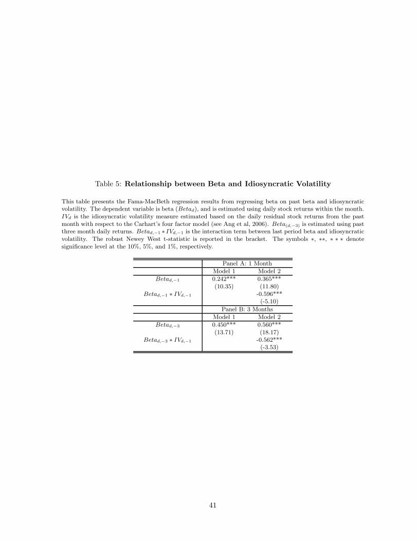
Table 5: Relationship between Beta and Idiosyncratic Volatility

This table presents the Fama-MacBeth regression results from regressing beta on past beta and idiosyncraticvolatility. The dependent variable is beta (Betad), and is estimated using daily stock returns within the month.IVd is the idiosyncratic volatility measure estimated based on the daily residual stock returns from the pastmonth with respect to the Carhart’s four factor model (see Ang et al, 2006). Beta(d,−3) is estimated using pastthree month daily returns. Betad,−1 ∗ IVd,−1 is the interaction term between last period beta and idiosyncraticvolatility. The robust Newey West t-statistic is reported in the bracket. The symbols ∗, ∗∗, ∗ ∗ ∗ denotesignificance level at the 10%, 5%, and 1%, respectively.

Panel A: 1 Month

Model 1 Model 2

Betad,−1 0.242*** 0.365***(10.35) (11.80)

Betad,−1 ∗ IVd,−1 -0.596***(-5.10)

Panel B: 3 Months

Model 1 Model 2

Betad,−3 0.450*** 0.560***(13.71) (18.17)

Betad,−3 ∗ IVd,−1 -0.562***(-3.53)

41

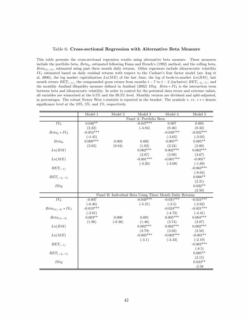
Table 6: Cross-sectional Regression with Alternative Beta Measure

This table presents the cross-sectional regression results using alternative beta measure. These measuresinclude the portfolio beta, Betap, estimated following Fama and French’s (1992) method, and the rolling beta,Beta(d,−3), estimated using past three month daily returns. Other regressors include idiosyncratic volatilityIVd estimated based on daily residual returns with respect to the Carhart’s four factor model (see Ang etal, 2006), the log market capitalization Ln(ME) of the last June, the log of book-to-market Ln(BM), lastmonth return RET(−1) , the compounded gross return from months t − 7 to t − 2 (inclusive) RET(−2,−7) , andthe monthly Amihud illiquidity measure defined in Amihud (2002) Illiq. Beta ∗ IVd is the interaction termbetween beta and idiosyncratic volatility. In order to control for the potential data errors and extreme values,all variables are winsorized at the 0.5% and the 99.5% level. Monthly returns are dividend and split-adjusted,in percentages. The robust Newey West t-statistic is reported in the bracket. The symbols ∗, ∗∗, ∗ ∗ ∗ denotesignificance level at the 10%, 5%, and 1%, respectively.

Model 1 Model 2 Model 3 Model 4 Model 5

Panel A: Portfolio Beta

IVd 0.046** -0.047*** 0.007 0.005(2.22) (-4.84) (0.46) (0.32)

Betap ∗ IVd -0.054*** -0.038*** -0.032***(-4.45) (-3.65) (-3.03)

Betap 0.009*** 0.003 0.002 0.005** 0.005**(3.03) (0.84) (1.02) (2.24) (2.00)

Ln(BM) 0.002*** 0.002*** 0.002***(3.87) (3.99) (3.67)

Ln(ME) -0.001*** -0.001*** -0.001*(-3.26) (-3.09) (-1.69)

RET(−1) -0.063***(-8.64)

RET(−2,−7) 0.006**(2.21)

Illiq 0.032**(2.50)

Panel B: Individual Beta Using Three Month Daily Returns

IVd -0.007 -0.049*** -0.031*** -0.024***(-0.46) (-5.21) (-3.5) (-2.62)

Beta(d,−3) ∗ IVd -0.019*** -0.024*** -0.021***(-3.81) (-4.72) (-4.41)

Beta(d,−3) 0.003** 0.000 0.001 0.005*** 0.004***(1.96) (-0.36) (1.46) (3.74) (3.07)

Ln(BM) 0.002*** 0.002*** 0.002***(3.79) (3.93) (3.58)

Ln(ME) -0.002*** -0.002*** -0.001**(-3.1) (-3.43) (-2.19)

RET(−1) -0.062***(-8.5)

RET(−2,−7) 0.005**(2.15)

Illiq 0.033**-2.58

42

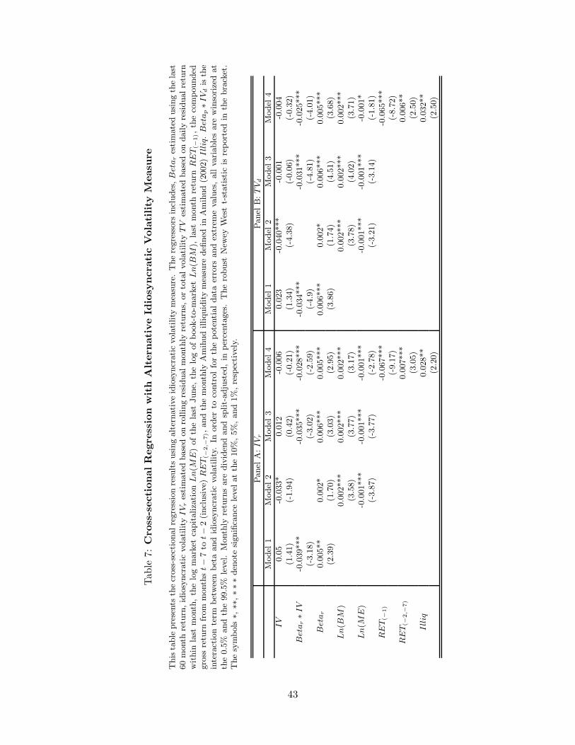
Tab

le7:

Cro

ss-s

ecti

onal

Reg

ress

ion

wit

hA

lter

nat

ive

Idio

syncr

atic

Vol

atility

Mea

sure

This

table

pre

sents

the

cross

-sec

tionalre

gre

ssio

nre

sult

susi

ng

alt

ernati

ve

idio

syncr

ati

cvola

tility

mea

sure

.T

he

regre

ssors

incl

udes

,B

eta

res

tim

ate

dusi

ng

the

last

60

month

retu

rn,id

iosy

ncr

ati

cvola

tility

IV

res

tim

ate

dbase

don

rollin

gre

sidualm

onth

lyre

turn

s,or

tota

lvola

tility

TV

esti

mate

dbase

don

daily

resi

dualre

turn

wit

hin

last

month

,th

elo

gm

ark

etca

pit

aliza

tion

Ln(M

E)

of

the

last

June,

the

log

of

book-t

o-m

ark

etL

n(B

M),

last

month

retu

rnR

ET

(−1),th

eco

mpounded

gro

ssre

turn

from

month

st−

7to

t−

2(i

ncl

usi

ve)

RE

T(−

2,−

7),and

the

month

lyA

mih

ud

illiquid

ity

mea

sure

defi

ned

inA

mih

ud

(2002)

Illiq

.B

eta

p∗I

Vd

isth

ein

tera

ctio

nte

rmbet

wee

nbet

aand

idio

syncr

ati

cvola

tility

.In

ord

erto

contr

ol

for

the

pote

nti

aldata

erro

rsand

extr

eme

valu

es,

all

vari

able

sare

win

sori

zed

at

the

0.5

%and

the

99.5

%le

vel

.M

onth

lyre

turn

sare

div

iden

dand

split-

adju

sted

,in

per

centa

ges

.T

he

robust

New

eyW

est

t-st

ati

stic

isre

port

edin

the

bra

cket

.T

he

sym

bols

∗,∗∗

,∗∗

∗den

ote

signifi

cance

level

at

the

10%

,5%

,and

1%

,re

spec

tivel

y.

Panel

A:IV

rPanel

B:T

Vd

Model

1M

odel

2M

odel

3M

odel

4M

odel

1M

odel

2M

odel

3M

odel

4

IV

0.0

5-0

.033*

0.0

12

-0.0

06

0.0

23

-0.0

40***

-0.0

01

-0.0

04

(1.4

1)

(-1.9

4)

(0.4

2)

(-0.2

1)

(1.3

4)

(-4.3

8)

(-0.0

6)

(-0.3

2)

Bet

ar∗I

V-0

.039***

-0.0

35***

-0.0

28***

-0.0

34***

-0.0

31***

-0.0

25***

(-3.1

8)

(-3.0

2)

(-2.5

9)

(-4.9

)(-

4.8

1)

(-4.0

1)

Bet

ar

0.0

05**

0.0

02*

0.0

06***

0.0

05***

0.0

06***

0.0

02*

0.0

06***

0.0

05***

(2.3

9)

(1.7

0)

(3.0

3)

(2.9

5)

(3.8

6)

(1.7

4)

(4.5

1)

(3.6

8)

Ln(B

M)

0.0

02***

0.0

02***

0.0

02***

0.0

02***

0.0

02***

0.0

02***

(3.5

8)

(3.7

7)

(3.1

7)

(3.7

8)

(4.0

2)

(3.7

1)

Ln(M

E)

-0.0

01***

-0.0

01***

-0.0

01***

-0.0

01***

-0.0

01***

-0.0

01*

(-3.8

7)

(-3.7

7)

(-2.7

8)

(-3.2

1)

(-3.1

4)

(-1.8

1)

RE

T(−

1)

-0.0

67***

-0.0

65***

(-9.1

7)

(-8.7

2)

RE

T(−

2,−

7)

0.0

07***

0.0

06**

(3.0

5)

(2.5

0)

Illiq

0.0

28**

0.0

32**

(2.2

0)

(2.5

0)

43

Tab

le8:

Cro

ss-s

ecti

onal

Reg

ress

ion

inD

iffer

ent

Mar

kets

This

table

pre

sents

the

Fam

a-M

acB

eth

regre

ssio

nre

sult

sfo

rdiff

eren

tst

ock

exch

anges

.T

hes

ere

gre

ssors

incl

udes

,B

eta

res

tim

ate

dusi

ng

the

last

60

month

lyre

turn

,id

iosy

ncr

ati

cvola

tility

IV

des

tim

ate

dbase

don

the

daily

resi

dualst

ock

retu

rns

from

the

past

month

wit

hre

spec

tto

the

Carh

art

’sfo

ur

fact

or

model

(see

Ang

etal,

2006),

the

log

mark

etca

pit

aliza

tion

Ln(M

E)

of

the

last

June,

the

log

of

book-t

o-m

ark

etL

n(B

M),

last

month

retu

rnR

ET

(−1),

the

com

pounded

gro

ssre

turn

from

month

st−

7to

t−

2(i

ncl

usi

ve)

RE

T(−

2,−

7),and

the

month

lyA

mih

ud

illiquid

ity

mea

sure

defi

ned

inA

mih

ud

(2002)

Illiq

.B

eta

p∗I

Vd

isth

ein

tera

ctio

nte

rmbet

wee

nbet

aand

idio

syncr

ati

cvola

tility

.In

ord

erto

contr

ol

for

the

pote

nti

aldata

erro

rsand

extr

eme

valu

es,

all

vari

able

sare

win

sori

zed

at

the

0.5

%and

the

99.5

%le

vel

.M

onth

lyre

turn

sare

div

iden

dand

split-

adju

sted

,in

per

centa

ges

.T

he

robust

New

eyW

est

t-st

ati

stic

isre

port

edin

the

bra

cket

.T

he

sym

bols

∗,∗∗

,∗∗

∗den

ote

signifi

cance

level

at

the

10%

,5%

,and

1%

,re

spec

tivel

y.

Panel

A:N

YSE

Panel

B:A

ME

X&

NA

SD

AQ

Model

1M

odel

2M

odel

3M

odel

4M

odel

5M

odel

1M

odel

2M

odel

3M

odel

4M

odel

5

IV

d0.0

22

-0.0

51***

-0.0

09

-0.0

18

-0.0

1-0

.034***

-0.0

17

-0.0

20

(1.0

7)

(-5.0

3)

(-0.6

)(-

1.1

6)

(-0.8

3)

(-3.8

3)

(-1.4

6)

(-1.5

2)

Bet

ar∗I

Vd

-0.0

39***

-0.0

35***

-0.0

25***

-0.0

13***

-0.0

15***

-0.0

10**

(-3.9

1)

(-3.6

9)

(-2.7

5)

(-2.9

5)

(-3.0

3)

(-2.0

6)

Bet

ar

0.0

05***

0.0

01

0.0

01

0.0

05***

0.0

04**

0.0

03**

0.0

00.0

02

0.0

05***

0.0

03*

(3.1

1)

(0.4

4)

(1.2

7)

(3.2

7)

(2.5

1)

(2.0

3)

(0.0

0)

(1.3

6)

(2.7

7)

(1.8

7)

Ln(B

M)

0.0

02***

0.0

02***

0.0

02***

0.0

04***

0.0

04***

0.0

04***

(3.2

8)

(3.4

5)

(3.1

5)

(5.4

9)

(5.5

7)

(4.9

1)

Ln(M

E)

-0.0

01***

-0.0

01***

-0.0

01*

-0.0

01*

-0.0

01**

0.0

00

(-3.0

6)

(-3.0

0)

(-1.9

3)

(-1.8

3)

(-2.0

0)

(-0.7

3)

RE

T(−

1)

-0.0

58***

-0.0

55***

(-6.9

3)

(-9.4

8)

RE

T(−

2,−

7)

0.0

07***

0.0

01

(2.6

0)

(0.5

3)

Illiq

0.0

40***

0.0

19***

(2.9

9)

(2.7

7)

44

Tab

le9:

Cro

ss-s

ecti

onal

Reg

ress

ion

Res

ult

sov

erD

iffer

ent

Subsa

mple

Per

iods

This

table

pre

sents

the

Fam

a-M

acB

eth

regre

ssio

nre

sult

sov

erdiff

eren

tsu

bsa

mple

per

iods.

Thes

ere

gre

ssors

incl

udes

,B

eta

res

tim

ate

dusi

ng

the

last

60

month

lyre

turn

,id

iosy

ncr

ati

cvola

tility

IV

des

tim

ate

dbase

don

the

daily

resi

dualst

ock

retu

rns

from

the

past

month

wit

hre

spec

tto

the

Carh

art

’sfo

ur

fact

or

model

(see

Ang

etal,

2006),

the

log

mark

etca

pit

aliza

tion

Ln(M

E)

of

the

last

June,

the

log

of

book-t

o-m

ark

etL

n(B

M),

last

month

retu

rnR

ET

(−1),

the

com

pounded

gro

ssre

turn

from

month

st−

7to

t−

2(i

ncl

usi

ve)

RE

T(−

2,−

7),and

the

month

lyA

mih

ud

illiquid

ity

mea

sure

defi

ned

inA

mih

ud

(2002)

Illiq

.B

eta

p∗I

Vd

isth

ein

tera

ctio

nte

rmbet

wee

nbet

aand

idio

syncr

ati

cvola

tility

.In

ord

erto

contr

ol

for

the

pote

nti

aldata

erro

rsand

extr

eme

valu

es,

all

vari

able

sare

win

sori

zed

at

the

0.5

%and

the

99.5

%le

vel

.M

onth

lyre

turn

sare

div

iden

dand

split-

adju

sted

,in

per

centa

ges

.T

he

robust

New

eyW

est

t-st

ati

stic

isre

port

edin

the

bra

cket

.T

he

sym

bols

∗,∗∗

,∗∗

∗den

ote

signifi

cance

level

at

the

10%

,5%

,and

1%

,re

spec

tivel

y.

Panel

A:1963-1

986

Panel

B:1987-2

010

Model

1M

odel

2M

odel

3M

odel

4M

odel

5M

odel

1M

odel

2M

odel

3M

odel

4M

odel

5

IV

r0.0

48

-0.0

67***

0.0

02

0.0

04

0.0

01

-0.0

27***

-0.0

12

-0.0

19

(1.4

0)

(-4.8

7)

(0.1

0)

(0.1

6)

(0.0

6)

(-2.9

5)

(-0.9

4)

(-1.4

8)

Bet

ap∗I

Vr

-0.0

60***

-0.0

54***

-0.0

45***

-0.0

15***

-0.0

14***

-0.0

08*

(-4.5

1)

(-4.1

7)

(-3.6

6)

(-3.1

3)

(-2.9

)(-

1.8

4)

Bet

ap

0.0

07**

0.0

00

0.0

01

0.0

06**

0.0

05**

0.0

04**

0.0

01

0.0

02

0.0

05***

0.0

04**

(2.4

7)

(0.0

3)

(0.5

8)

(2.5

3)

(2.2

1)

(1.9

8)

(0.7

5)

(1.6

0)

(2.6

9)

(2.0

0)

Ln(B

M)

0.0

02**

0.0

02**

0.0

02**

0.0

03***

0.0

03***

0.0

03***

(1.9

8)

(2.1

6)

(2.1

3)

(3.6

3)

(3.7

6)

(3.3

1)

Ln(M

E)

-0.0

02***

-0.0

02**

-0.0

01*

-0.0

01**

-0.0

01**

-0.0

01

(-2.6

7)

(-2.5

5)

(-1.6

7)

(-2.4

2)

(-2.4

6)

(-1.2

)R

ET

(−1)

-0.0

81***

-0.0

49***

(-7.5

)(-

7.7

7)

RE

T(−

2,−

7)

0.0

10***

0.0

02

(3.4

7)

(0.6

3)

Illiq

0.0

41*

0.0

25***

(1.6

6)

(3.1

3)

45

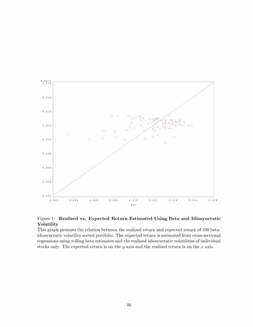
E ( R e t )

0 . 0 0 2

0 . 0 0 4

0 . 0 0 6

0 . 0 0 8

0 . 0 1 0

0 . 0 1 2

0 . 0 1 4

0 . 0 1 6

0 . 0 1 8

R e t

0 . 0 0 2 0 . 0 0 4 0 . 0 0 6 0 . 0 0 8 0 . 0 1 0 0 . 0 1 2 0 . 0 1 4 0 . 0 1 6 0 . 0 1 8

Figure 1: Realized vs. Expected Return Estimated Using Beta and IdiosyncraticVolatilityThis graph presents the relation between the realized return and expected return of 100 beta-idiosyncratic volatility sorted portfolio. The expected return is estimated from cross-sectionalregressions using rolling beta estimates and the realized idiosyncratic volatilities of individualstocks only. The expected return is on the y axis and the realized return is on the x axis.

46

E ( R e t )

0 . 0 0 2

0 . 0 0 4

0 . 0 0 6

0 . 0 0 8

0 . 0 1 0

0 . 0 1 2

0 . 0 1 4

0 . 0 1 6

0 . 0 1 8

R e t

0 . 0 0 2 0 . 0 0 4 0 . 0 0 6 0 . 0 0 8 0 . 0 1 0 0 . 0 1 2 0 . 0 1 4 0 . 0 1 6 0 . 0 1 8

Figure 2: Realized vs. Expected Return Estimated Using Beta, IdiosyncraticVolatility and Interaction TermThis graph presents the relation between the realized return and expected return of 100beta-idiosyncratic volatility sorted portfolio. The expected return is estimated from cross-sectional regressions using rolling beta estimates, the realized idiosyncratic volatilities, andthe interaction between beta and idiosyncratic volatility of individual stocks. The expectedreturn is on the y axis and the realized return is on the x axis.

47