NPL REPORT MAT 65

NPL REPORT MAT 65 Best practice guide for the generation and measurement of DC magnetic fields in the magnetic field range of 1 nT to 1 mT Dr Michael Hall, Steven Turner and Stuart Harmon from NPL Sylke Bechstein, Dr Thomas Schurig and Dr Martin Albrecht from PTB Michal Janosek and Aleš Zikmund from CTU in Prague Michal Ulvr and Dr Josef Kupec from CMI JUNE 2014

NPL REPORT MAT 65

i

Best practice guide for the generation and measurement of DC magnetic fields in the magnetic field range of 1 nT to 1 mT

Dr Michael Hall, Steven Turner and Stuart Harmon from NPL Sylke Bechstein, Dr Thomas Schurig and Dr Martin Albrecht from PTB

Michal Janosek and Aleš Zikmund from CTU in Prague Michal Ulvr and Dr Josef Kupec from CMI

NPL REPORT MAT 65

ii

Queen’s Printer and Controller of HMSO, 2014

ISSN 1754-2979

National Physical Laboratory Hampton Road, Teddington, Middlesex, TW11 0LW

Extracts from this report may be reproduced provided the source is acknowledged and the extract is not taken out of context.

Approved on behalf of NPLML by Neil Olds, Director of the Materials Division.

NPL REPORT MAT 65

iii

Best practice guide for the generation and measurement of DC magnetic fields in the magnetic field range of 1 nT to 1 mT

Scope of guide The object of this guide is to define the general principles and the technical details of the generation and measurement of DC magnetic fields in the range 1 nT to 1 mT. Calibration at temperatures in the range - 55 ºC to 125 ºC will be described along with calibration methods for 3 axis magnetometers. After introducing the facilities that are required to establish the necessary ambient magnetic field conditions, methods for generating magnetic fields with the required range and uniformity will be explained. This will include aspects such as the size and geometry of the coil system necessary to establish a suitably uniform field through the volume of the sensor. How the coil systems and customer magnetometers are calibrated and the uncertainties of these calibrations established will be covered along with typical additional uncertainties that need to be considered when the magnetometer is used in an industrial location. Examples of European facilities and measurement case studies will be used to demonstrate these principles.

NPL REPORT MAT 65

iv

Contents

Best practice guide for the generation and measurement of DC magnetic fields in the magnetic field range of 1 nT to 1 mT ..............................................................................................................................iii

Scope of guide ........................................................................................................................................iii

Introduction.............................................................................................................................................. 1

Concepts and general principles ............................................................................................................. 1

Units and SI/CGS conversion ............................................................................................................. 1

Magnetic environment ............................................................................................................................. 3

Location and design considerations .................................................................................................... 3

Cancellation systems .......................................................................................................................... 5

Remote reference magnetometer ................................................................................................... 5

Magnetically screened environments .............................................................................................. 7

Field generating methods ........................................................................................................................ 9

Helmholtz coils .................................................................................................................................... 9

Solenoids........................................................................................................................................... 12

Gradient coils .................................................................................................................................... 13

Astatic coils ....................................................................................................................................... 15

Modelling of field at a distance ...................................................................................................... 15

Fabrication of astatic coil system .................................................................................................. 16

Measurements of field at a distance ............................................................................................. 16

Three axis coil systems ..................................................................................................................... 18

Field Measuring methods ...................................................................................................................... 18

DC SQUID magnetometer ................................................................................................................ 18

Fluxgate magnetometers .................................................................................................................. 19

Proton precession magnetometers ................................................................................................... 21

Atomic magnetometers ..................................................................................................................... 22

Measurement parameters ..................................................................................................................... 23

Gain ................................................................................................................................................... 23

Linearity ............................................................................................................................................. 24

DC offsets.......................................................................................................................................... 24

Noise ................................................................................................................................................. 24

Orthogonality ..................................................................................................................................... 25

AC field rejection ............................................................................................................................... 25

Measurements at elevated temperatures ......................................................................................... 25

Commercial systems ..................................................................................................................... 25

Design considerations ................................................................................................................... 25

Temperature chamber materials ................................................................................................... 25

NPL REPORT MAT 65

v

Temperature control ...................................................................................................................... 26

Uncertainty of measurement ................................................................................................................. 26

General principles ............................................................................................................................. 26

Sources of uncertainty ...................................................................................................................... 27

Statistical assessment of uncertainties ............................................................................................. 28

Measurement uncertainty for industrial locations ............................................................................. 29

Traceability ............................................................................................................................................ 30

European capabilities for low magnetic field measurements ................................................................ 30

References ............................................................................................................................................ 32

NPL REPORT MAT 65

1

Introduction Magnetic field measurements at flux density levels of 1 nT to 1 mT are required by industries ranging from deep space exploration to those involved with removing contamination from food products. An understanding of the principles of operation, calibration methods and limitations of the sensors and magnetometers used for these measurements is required so that dependant industries are in a sustainable position. This Best Practice Guide aims to provide industry end users, instrument manufactures and accredited Calibration Laboratories with a framework of understanding that underpins the measurements of such a vast range of uses. No written standards exist for these measurements and it is hoped that this Best Practice Guide will form the starting point of a standardisation programme.

This guide covers the environment necessary for magnetic measurements at the nT level, methods for generating magnetic fields, the various magnetometers used to measure magnetic fields and the typical parameters that are calibrated and concludes with a description of how to determine the uncertainties associated with the measurements.

When making magnetic field measurements in this range the contribution from the ambient magnetic environment can be a significant part of the measured field. Advice will be given on how to make these measurements when it is not possible to reduce these contributions significantly.

Concepts and general principles

Units and SI/CGS conversion SI units should be used at all times. Since there are many text books that use older systems of units, the following explains the conversion factors needed to change between them.

To the uninitiated, magnetic measurements seem to be shrouded in mystery. It is apparent that confusion exists in understanding the fundamental definitions and units. This is not at all surprising since there has been a proliferation of unit systems and these have affected the field of magnetism perhaps more than any other branch of physics. Even in the two main unit systems, CGS and SI, there have been changes; the situation is summarised in the following Table 1:

NPL REPORT MAT 65

2

Table 1

Quantity

CGS unit

SI unit

1900-1932

1933-1953

1954-1959

1960-1986 magnetic field strength, H

gauss

oersted

ampere/metre

ampere/metre

magnetic flux density, B and magnetic polarisation, J

gauss

gauss

weber/metre2

tesla

magnetic constant, μo

1

1

henry/metre

henry/metre

magnetic flux, Φ

maxwell

maxwell

weber

weber

Note: In geomagnetism, the unit "gamma" is used. In the CGS system 1 gamma is equivalent to 10-5 oersted, however in SI units it is deemed to be 1 nanotesla. In the International System of Units (SI), magnetic units depend upon the fundamental units of length (metre), mass (kilogram), time (second) and upon the definition of the ampere, based upon Ampere's law for the force between two current carrying conductors: "If two straight parallel conductors a distance d apart carry currents I1 and I2 the force, F, between them per unit length in rationalised units is given by: F = μoI1I2/2πd 1 where μo is a constant called the magnetic constant (permeability of free space)". From the definition of the ampere, the value of the magnetic constant (permeability of free space) in SI units is: μo = 4π x 10-7 (henry/metre) 2 The definition of magnetic flux density (magnetic induction), B, is related to the force exerted on a current carrying conductor in a magnetic field, normal to the direction of that field. If the current is I, the force, F, per unit length is the vector product of B and I: F = B x I (newton/metre) 3 The dimensional equation gives: N/m = [B] A 4 thus:

[𝐵] = 𝑛𝑒𝑤𝑡𝑜𝑛𝑎𝑚𝑝.𝑚𝑒𝑡𝑟𝑒

= 𝑤𝑎𝑡𝑡.𝑠𝑒𝑐𝑜𝑛𝑑𝑎𝑚𝑝.𝑚𝑒𝑡𝑟𝑒2

= 𝑣𝑜𝑙𝑡.𝑠𝑒𝑐𝑜𝑛𝑑𝑚𝑒𝑡𝑟𝑒2

= 𝑤𝑒𝑏𝑒𝑟𝑚𝑒𝑡𝑟𝑒2

= 𝑡𝑒𝑠𝑙𝑎 5

The magnetic field strength (magnetic field, magnetising force), H, can be defined in free space by the expression:

NPL REPORT MAT 65

3

B = μoH 5 that is, H is the magnetic vector quantity at a point in a magnetic field which measures the ability of electric currents or magnetized bodies to produce a magnetic flux density at that point. The dimensional equation gives: [H] = T/Hm-1 6 thus:

[𝐻] =𝑣𝑜𝑙𝑡.𝑠𝑒𝑐𝑜𝑛𝑑𝑚𝑒𝑡𝑟𝑒2

𝑣𝑜𝑙𝑡.𝑠𝑒𝑐𝑜𝑛𝑑𝑎𝑚𝑝𝑒𝑟𝑒.𝑚𝑒𝑡𝑟𝑒

� = 𝑎𝑚𝑝𝑒𝑟𝑒𝑚𝑒𝑡𝑟𝑒

7

The more common conversions of units between SI and CGS are given in Table 2.

Table 2

Quantity SI CGS

Magnetic field strength, H 1 A/m 0.012566 Oe 79.58 A/m 1 Oe

Magnetic flux density, B 1 T 10000 Gs 0.0001 T 1 Gs

Magnetic environment

Location and design considerations Due to the nature of the measurements made in low field laboratories, there are few locations near built up areas that are suitable since the magnetic field gradients and variations in magnetic field are too large to be sufficiently compensated. An older brick construction or wooden building is necessary due to the use of mild steel in modern building construction and should be sited in as remote a location as possible.

For a laboratory to achieve the required level of performance for these measurements, it is necessary to locate it away from sources of man-made magnetic field and electromagnetic interference. Examples of such fields are the movement of vehicles, people, elevators and buildings constructed of modern building materials such as mild steel. All of these will produce locally varying magnetic fields that cannot be removed due to the resulting magnetic field gradient. Within the laboratory it is necessary to remove all ferrous materials.

The location considered for calibration campaigns should be at least 10 km from DC railway lines, 5 km from subway or tramway lines. Otherwise up to 50 nT p-p low-frequency peaks may be observed. If the area is geologically difficult, those fields can be also of highly gradient character complicating the use of field cancelling systems. Avoid also the vicinity of high-pressure gas piping or

NPL REPORT MAT 65

4

other metallic piping. If the site is not located within one mile of AC power lines then no significant local DC currents will be introduced by ground currents and load asymmetries. The field conditions on site should be checked with a proton/Overhauser magnetometer together with 3-axial fluxgate and the data should be compared to the nearest INTERMAGNET observatory data. If the location is not ideal measurements should be taken at assessable minima such as night / early morning and/or sufficient averaging has to be used, although this will not guarantee adequate precision. The location should also minimize temperature drifts, i.e. provide shadow during the day. Care must be taken for stray fields using active air conditioning.

The following details give approximations to indicate the scale of the requirements. They are based on the facility at NPL and could also be those of equivalent facilities elsewhere. For other facilities the details will vary but the information below establishes the main requirements. Individual requirements will be different and may compromise the operational range and associated uncertainties.

• An ambient magnetic field variation with time that is no worse than that shown in Figure 3. • A room for the main coil system and associated field standards that is sufficiently large (in

the case of NPL this is 8 m by 8 m by 8 m). Temperature should be controlled in this space to ± 1 °C during testing using a system containing no ferrous parts. The actual temperature is usually between 19 and 24 °C and should be agreed prior to starting the measurements.

• A control room for the hardware used at a distance far enough away to avoid interaction between the coil system and the electronics (in the case of NPL this is 3 m by 3 m by 3 m and is 25 m from the main laboratory).

• For a remote magnetometer based system (see Figure 2) such as the cancellation system at NPL, a magnetically clean and hermetically sealed space is used for the reference magnetometer. The distance to the coil system should be as small as possible, but, it must ensure that there is no measurable influence of the stray field of the coil system at the location of the remote magnetometer (usually that is no closer than 70 m from the main laboratory for a Helmholtz-coil system).

• Watertight conduits between these rooms and spaces for supply and signal cables • All rooms must be constructed of non-magnetic materials with the main laboratory being on

solid foundations • Field cancellation system should be constructed from non-magnetics materials, either

aluminium frame or paper based such as Fibrelam • Ability to level the horizontal axis of the main coil system. • No cars closer than 100 m to the main laboratory, control room and reference magnetometer

space • No people traffic closer than 30 m to the main laboratory and reference magnetometer space

To illustrate the building requirement for such a facility, the NPL Low Magnetic Field Laboratory is based in an old building and unlike modern buildings, when built in 1663 no magnetic materials were used in the construction. As a consequence, the magnetic signature of the building is very small. This made the building suitable for a low magnetic field laboratory based on coil systems to reduce the ambient magnetic field to the required level. The downside to the NPL location is the influence from the local electric train service where the third rail ground currents produce variations in the local ambient magnetic field. Although the system has been modified to operate within this environment the ideal situation would be to locate a laboratory as far away from such sources of ambient variation so that there is no influence on the measurements performed.

The remote reference magnetometer system shown in Figure 2 is operated at NPL where the remote magnetometer is located approximately 70 m away from the reference magnetometer in the laboratory. The gradient between the monitoring magnetometer based in the main laboratory and the remote magnetometer has been determined to be 1.3 nT/m and is shown in Figure 1 below. At this distance the interaction between the two magnetometers is negligible, but any increase in distance would lead to a larger total difference between the two locations.

NPL REPORT MAT 65

5

Figure 1. Gradient measured at the NPL low magnetic field laboratory.

Cancellation systems

Remote reference magnetometer Using a reference magnetometer to cancel the fixed component and variations in the Earth’s ambient magnetic field requires and environment where the magnetic gradients are as low as possible over a reasonably large distance. The compromise is to locate the remote magnetometer so that the difference between it and the reference magnetometer is negligible but also so that the interaction between the two is also negligible. Generally the distance between the two magnetometers is of the order of 10’s of meters.

The following describes the NPL Low Field Cancellation system as an example.

Cancellation is achieved using a reference three axis fluxgate magnetometer. The experimental layout is shown in Figure 2.

30

40

50

60

70

80

90

10 20 30 40 50 60

From straight line fit, the gradient is 1.3 nT / m.

y = +1.29638x1 +3.97470, max dev:11.5003, r2=0.922486

The Y axis is determined by first taking the difference between the measured magneticfields at a fixed point and a point X meters away.The Max and Min difference is then determined for the residuals obtained.

Distance X, (m)Max

and

Min

diff

eren

ce b

etwe

en th

e m

easu

red

mag

netic

fiel

ds (n

T) Bushy House existing location

NPL REPORT MAT 65

6

Figure 2. Schematic showing the cancellation method used.

The remote reference magnetometer is 70 m from the triaxial Helmholtz coil and is used to generate currents in each of its three axes to cancel the fixed component in that direction. The smaller time variations are removed by adjusting these currents using an identical magnetometer at the centre of the triaxial Helmholtz coils in the main laboratory. This magnetometer is then removed during calibrations.

Using this approach a noise floor of 20 pT/√Hz at 1 Hz is achieved within a spherical volume of 150 mm at the centre of the triaxial coil system.

Shown in Figure 3 is the magnetic field variation in the laboratory before and after cancellation. The black curve was measured by the remote magnetometer and shows the field variations that also occur in the main laboratory where the cancellation is operated. The origins of the variations with time before the cancellation system is operated are mainly due to the electric train system used in the area. The electrical return of the circuit is not insulated and so earth leakage currents are generated causing a variation mainly in the vertical component. These currents then produce the very small magnetic fields shown in Figure 3. Other sources of disturbance in the ambient magnetic field are from the Earth’s daily diurnal variation, ‘Sun Spot’ activity and the effect of vehicles and other nearby ferromagnetic items.

X

Y

Z

X

Y

Z

Servo controlinputs

Keithley DVM's

Outputs frommagnetometer

Fluxgatemagnetometer

Fluxgate probe Kepco power supplies

supplementarypower supply

Remotefluxgate probe

Remote fluxgatemagnetometer

supplementarypower supply

Triaxialcoil

system

NPL REPORT MAT 65

7

Figure 3. Cancellation achieved with existing system.

As more sensitive magnetometers are developed the noise floor of Fluxgate based cancellation systems needs to be lowered to 1 pT/√Hz at 1 Hz. This can be achieved by using atomic magnetometers to lower the measurement noise floor from the 7 pT/√Hz at 1 Hz limit currently achieved using low noise fluxgate magnetometers.

Magnetically screened environments Magnetic shielding can be used to reduce the ambient magnetic field to very low levels. This approach is only suitable if magnetic fields are not to be generated in the cancelled space. This is because magnetic images generated in the material of the shielding as a result of the very high magnetic permeability alter the behaviour of the shield as well as create unknown contributions to the magnetic field being generated.

To determine the noise of a magnetometer at very low frequencies of 1 mHz or less it is necessary to use a shielded environment. This is because the stability of the cancelled field obtained using a coil system is not sufficient for the very long measurement runs necessary. For example, to measure noise at 0.1 mHz it is necessary to measure the output(s) of the magnetometer for at least 70000 seconds. This corresponds to 7 cycles and using less than this will lead to artefacts in the Logarithmic Power Spectral Density (LPSD) calculation used to determine the noise.

When the output of the magnetometer is sensitive to temperature, it is also necessary to maintain a very stable temperature. If this is not the case, slow drifts in the output(s) of the magnetometer due to temperature will contribute to the noise measurement at these frequencies.

-75

-60

-45

-30

-15

0

15

30

0 120 240 360 480 600 720 840 960 1080

Remote magnetometerLaboratory Magnetometer

Time (s)

Mag

netic

flux

den

sity

(nT)

NPL REPORT MAT 65

8

Shown in Figure 4 is the outer can of a three layer can used to measure noise at 0.1 mHz. This has been placed inside the NPL cancellation system to reduce the ambient variation to an already low level.

Figure 4. Noise measurements at 0.1 mHz.

To measure the LPSD shown in Figure 5, this was placed inside a thermal isolation box that achieved a temperature stability of ± 0.05 °C for the measurement time of at least 70000 seconds.

NPL REPORT MAT 65

9

Figure 5. LPSD for determining noise at 0.1 mHz.

For the PSD in Figure 5 the noise at 0.1 mHz is (475 ± 220) pT/√Hz. This was measured using a fluxgate magnetometer and the noise is probably limited by the magnetometer and not the environment. To determine if the noise of the environment is less than this, a SQUID magnetometer would be needed.

Field generating methods

Helmholtz coils Helmholtz coils are used to generate a uniform region of magnetic field along the axis of the coil. When the separation, s, of two identical coils is equal to the radius r, the Helmholtz condition is satisfied. A typical setup is shown in Figure 6 where:

S is the separation between coil 1 and coil 2,

R is the coil radius,

A is the distance from each coil to the mid-plane, a = s/2,

100

200

500

0.0001 0.001 0.01

Frequency [Hz]

Mag

neto

met

er o

utpu

t (pT

/√Hz

)

NPL REPORT MAT 65

10

Figure 6. Diagram of the arrangement of Helmholtz coils.

For the lowest uncertainty, the coil constant, defined as the ratio of the magnetic field strength to the current in the coils, is determined at DC using a resonance method. The required field strength is then established by calculating the current needed to generate the field, and measuring the current using a calibrated resistor and calibrated digital voltmeter (DVM).

In a pair of Helmholtz coils, the accuracy of the magnetic fields produced within them is primarily affected by the accuracy with which they are constructed, and the accuracy with which the current driving them is known. The coil constant of Helmholtz coils is given by the relationship:

rN

IH

558

= 8

where

H is the axial magnetic field strength, in A/m,

I is the current in the coils, in A,

N is the number of turns on each coil,

R is the radius of each coil, in m,

The magnetometer to be calibrated is positioned coaxially and midway between the two Helmholtz coils, and aligned to produce maximum output voltage by monitoring this voltage as small rotations of the plane of the magnetometer are made. At the required magnetic field strength, the output reading of the magnetometer is recorded. When the output is an analogue voltage a calibrated DVM is used. The resistor voltage is recorded, and used to determine the coil current and the magnetic field. The percentage error caused by field non-uniformity along the length of the magnetometer and across the diameter can be found from Figure 7 and Figure 8 which are plots of the coil constant against the ratio of the radius of the magnetometer and the distance along the axis to the radius of the coils respectively.

NPL REPORT MAT 65

11

Figure 7. Variation of H/I along the x-axis (axis through the centre) of the coils.

Figure 8. Variation of H/I across the central plane (x = 0) between the coils.

0.975

0.980

0.985

0.990

0.995

1.000

0 0.1 0.2 0.3 0.4

Normalised distance, x/coil radius

Norm

alise

d H/

I

Helmholtz CoilsVariation for H/I along axis general case

0.990

0.995

1.000

0 0.1 0.2 0.3 0.4

Normalised distance, x/coil radius

Norm

alise

d H/

I

Helmholtz CoilsVariation for H/I across central plane general case

NPL REPORT MAT 65

12

When the windings have a finite width the uniformity can be improved by adjusting the spacing. Alternative coil arrangements that provide more homogeneous field regions like compensated coils can be used [1].

Equation 8 assumes that the “coils” are a single circle of wire of negligible cross-section. In practice they consist of a large number of turns of wire of adequate cross-section to carry the required current without undue heating, wound in grooves of width, w, and depth d. This condition is met when

5𝑎2

𝑐2− 1 + 4

75 𝑟2(31𝑑2 − 36𝑤2) 9

where c is the hypotenuse of a right angled triangle with sides of a and r.

One way of meeting this condition for optimum separation to provide good uniformity is to make the turns per layer equal to the number of layers and to separate the layers by plastic ribbon of thickness such as to increase the depth by the required amount. Although this solution, making the two terms of equation 10 vanish independently, is perhaps more elegant, it risks being impracticable if the material of the coil formers is available only in standard thicknesses. The alternative is to reduce the second term as far as possible with standard material, and change the coil separation 2a by an amount necessary to satisfy equation 10.

Solenoids They are many types of solenoids, with single layer or thick massive coils. Solenoids are very often constructed with several symmetrical sections so that magnetic field inside has greater homogeneity. According to their original authors their names are Helmholtz solenoid, Barker solenoid, Garrett coil and Montgomery massive coils. Homogeneity of magnetic flux density in the central space of such a coil system depends on the type of coil, relations of sections and its dimensions and is well described in literature.

A uniform region of magnetic field can also be produced by a solenoid.

For an infinitely long solenoid the magnetic field at the centre is given by:

𝐻 = 𝑛𝐼 10

Where n is the number of turns per meter and I the current in Amps.

More generally:

𝐻 = 𝑛𝐼𝑙/2

[𝑟2+𝑙24 ]1/2

11

where l is the length of the solenoid and r is the radius.

When (l/r) is at least 10, r2 is negligible compared to l2/4 and equation 11 is obtained.

NPL REPORT MAT 65

13

Gradient coils When calibrating gradiometers a gradient field standard is required that exhibits a constant gradient. One such coil is a Maxwell pair and this is shown in Figure 9.

The full gradient tensor is:

12

In the absence of local current

13

because ∇ × B = 0.

Also, since the magnetic gradient tensor is symmetric and has a zero trace

14

the number of independent components that need to be determined is 5.

Shown in Figure 9 is a gradient coil used to calibrate these components. This is a Maxwell coil and consists of two identical coils separated at a distance equal to the diameter.

NPL REPORT MAT 65

14

Figure 9. Gradient coil for the calibration of gradiometers.

For the calibration of the diagonal terms of the gradient tensor the coils shown in Figure 9 are connected so that the current is in opposite directions. The resulting magnetic gradient profile is shown in Figure 10.

Figure 10. Uniformity along the coil axis of the magnetic field gradient of the coil shown in Figure 9 for the Maxwell configuration. Zero is the midpoint between the coils.

Since the off diagonal components of the gradient tensor are zero for a Maxwell coil, it is necessary to connect the coils so that the current in each of the coils is in the same direction. For this Helmholtz configuration, the variation of Bx against increasing distance along Y is shown in Figure 11.

-0.035

-0.030

-0.025

-0.020

-0.015

-0.010

-0.005

0

0.005

0.010

0.015

-30 -25 -20 -15 -10 -5 0 5 10 15 20 25 30

Distance from centre (mm)

Chan

ge in

gra

dien

t fro

m v

alue

at c

entre

(%)

NPL REPORT MAT 65

15

Figure 11. Bx magnetic field profile against Y at X=0 for the coil shown in Figure 9 for the Helmholtz configuration of the coil current.

This is done by measuring the outputs of the fluxgate magnetometers that form the gradient pair as the gradiometer is moved in the increasing Y direction by known distances. By comparing the results to the curve in Figure 11, the effective spacing between the gradient pair can be determined. This baseline is then used to determine unknown off diagonal gradients components.

Astatic coils In certain situations it is necessary to prevent interference between field generating coils and a magnetometer. An example is the control loop of the single volume low magnetic field system discussed in this guide. Due to the separation between the magnetometer being calibrated (DUT) and the caesium magnetometer used to stabilise the field, each magnetometer will experience a small but significant difference in the field caused by the non-perfect homogeneity of the field of the Helmholtz coils. It is therefore necessary to keep this distance as small as possible to limit this difference. To correct for what remains, a coil is used to generate a biasing field. To provide optimum compensation the biasing field should not be detected by (or coupled to) the DUT. In practice any field generated by a coil system within the cancelled volume, although greatly reduced with distance, will still be present at the centre of the volume. An astatic coil is able to generate a magnetic field that falls-off (with distance) at a rate greater than that of the conventional cubic law.

Modelling of field at a distance An astatic coil is composed of two coplanar and co-centred coils connected in series opposition, where the dimensions are such that the optimum fall-off rate, for a coil of any size, is achieved when the criteria described by the following equation are met.

2211 ANAN = 15

7

8

9

10

0 50 100 150 200

Y (mm)

B (u

T)

Bx along Y at X=0

X

Y

Z

NPL REPORT MAT 65

16

Here the product of the number of turns, N, given as an integer and the area enclosed by the coil, A, for each coil must be equal. The subscripts 1 and 2 are used to distinguish between the two coils.

Using this equation, various coil configurations were modelled by applying the Biot-Savart engine from Opera 3D’s finite element modelling software. The influence of the windings width, length and the optimum spacing between coils were evaluated. This revealed that the maximum fall-off is achieved when the coil diameter, length and spacing between coils is minimal. Therefore to accommodate the number of turns required to generate a minimum 20 µT/A and minimise coil length, each coil is wound using multiple layers.

Table 3 shows the data generated from a batch analysis of coils using 2 mm diameter enamelled copper wire, a 200 µm thick insulator between coils and a minimum coil diameter of 0.14 m. The minimum coil diameter is restricted due to the field uniformity required across the volume of the feedback transducer, which for this application is a Caesium magnetometer. In addition to this there exists physical restriction placed on the minimum coil diameter, which must house the magnetometer at an angle of 45°. This tumble angle between the magnetometer’s optical axis and the field generated by the astatic coil is critical to the generation of a Lamour signal.

Table 3. Change in fall-off at a distance of 0.5 m from the coil centre, given as a percentage of the maximum field, for matched integer values of N1 and N2.

N1

(Turns) N2

(Turns) Fall-off

(%) 15 13 99.947 16 14 99.960 17 15 99.973 18 16 99.985 19 17 99.997 20 18 99.992

Fabrication of astatic coil system The finite element analysis found that, for the dimensions given above, an optimum fall-off rate of 99.997% at a distance of 0.5 m was achieved when 191 =N and 172 =N turns. Therefore a former

was fabricated from non-metallic materials (i.e. Acetal) using these dimensions and the 191 =N turns ratio. The actual coil was wound using solderable enamelled copper wire with a diameter of 2 mm giving the coil a maximum current carrying capacity of 11.5 A.

The innermost coil, N1, was comprised of two layers with 10 turns and 9 turns for the bottom and top layers respectively. The outermost coil, N2, was also comprised of two layers where the bottom layer had 9 turns and the top layer had 8 turns. A strip of 200 µm thick insulation paper was used to separate the two coils and provided a flat surface on which to wind the second coil.

Measurements of field at a distance For comparison, the outermost coil of the fabricated Astatic coil was electrically isolated and so only the innermost coil was used to generate approximately 50 µT in the centre of the coil from a 0.4 A DC supply current. This effectively represents a short-solenoid, which obeys the conventional cubic law and is comparable in size to the astatic coil.

The z-axis of a calibrated Bartington Mag03-MC70 fluxgate magnetometer was used to measure the magnetic flux density at 50 mm intervals from the centre of the solenoid and up to a distance of 0.5 m. The fluxgate’s core is actually made from relatively long strands of amorphous wire (i.e. 18 mm), and so its centre was determined by moving the fluxgate through the coil until a maximum output was

NPL REPORT MAT 65

17

observed. A calibrated 0.6 m steel rule was used to measure and mark out the distance between the centres of both the fluxgate and the coil.

All measurements were performed inside a triaxial cancellation system, where the magnitude and variations in the Earth’s magnetic field were reduced to minimize their contributions to the measured magnetic flux density. Due to the magnetic properties of the steel rule it was removed from the laboratory, along with all other magnetic materials (i.e. coins, belt buckles, keys, etc…), before performing any magnetic measurements.

At each 50 mm interval the fluxgate was aligned and rotated to give the maximum output from the z-axis and magnetic flux density was determined from an average of three measurements. To account for any residual offset, the polarity of the current supply was switch to reverse the direction of the field generated by the coil and the measurements were repeated at each interval. The offset can then be calculated from the difference between the flux density measured whilst applying the field in the forward and reverse directions.

This same procedure was repeated using both coils connected in series opposition to form an astatic coil. However, the electric current was increased to 2 A DC, in order to generate a 50 µT peak field. The results for both the Inner and astatic coils are shown in Figure 12.

The measured flux density generated by the astatic coil drops from 50.6 µT in the centre of the coil down to below 2 nT at a distance of 0.5 m. This represents a 99.997% fall-off and correlates well with the modelled data, which also exhibits a drop of 99.997%.

Figure 12. Comparison of flux density measured at a distance of up to 0.5 m, generated by (a) modelling and (b) measuring the 19 turn inner coil and the complete astatic coil.

NPL REPORT MAT 65

18

Three axis coil systems Triaxial coil systems should be built of appropriate material with low thermal expansion and rigid enough to prevent instability of angular misalignments. Non-conducting material is preferred because of possible eddy currents and the risk of electrical shorts. Multiple coil systems are preferred to Helmholtz coils because of the greater homogeneity.

Field Measuring methods

DC SQUID magnetometer SQUIDs (Superconducting QUantum Interference Devices) are the most sensitive detectors for magnetic flux changes presently available. With a typical spectral magnetic flux noise density of a few µΦ0/Hz½, SQUID magnetometers are for example used for the detection of biomagnetic signals generated by human or animal brain or heart activities. Other applications are geophysical/archaeological projects, or the non-destructive evaluation of material, e. g. magnetically shielded rooms or boxes can be evaluated with respect to residual fields and noise.

Both, the performance of the SQUID sensors and the scale of integration have been continuously improved in the last decades. By now, single sensors or small systems including the read out electronics are sold by SMBs, whereas large multi-channel systems have been developed and manufactured rather by research institutes.

SQUIDs always operate at temperatures below the critical temperature Tc of the superconductor, which depends on the applied material and the fabrication process. Most common dc SQUIDs are fabricated in conventional Nb/AlxOy/Nb trilayer technology. These SQUID magnetometers are mostly operated in low-noise liquid helium cryostats at a temperature of 4.2 K.

In principle, a dc SQUID magnetometer consists of a superconducting loop interrupted by two Josephson junctions (Figure 13b), whereas the loop of rf SQUIDs is interrupted by a single junction. Both types are described in [2]. If a SQUID is appropriately biased, the output voltage is a periodic function of the applied flux changes with the period of one flux quantum (Figure 13c, black). Basically, the SQUID acts as a non-linear flux-to-voltage converter. The conversion can be linearised by applying a Flux Locked Loop (FLL), in which the output signal is coupled back to the SQUID via a feedback circuitry. Thus the SQUID keeps locked in the working point W.

Figure 13. (a) Example of SQUID chip. (b) Scheme of dc SQUID. (c) Output voltage V for a steadily increased magnetic flux Φ. The period is associated with one flux quantum Φ0.

A well known design for a SQUID magnetometer is the thin-film multi-turn SQUID or ‘cartwheel SQUID’, developed in 1990 by D. Drung at PTB [3]. Another method for magnetometer application is the combination of a current sensor and a pickup coil, whereas the coil can be wire wounded or integrated on chip. For extremely low-noise applications, a two-stage configuration may be useful, where the signal of the SQUID sensor is pre-amplified by a SQUID amplifier.

(c) (b) (a)

NPL REPORT MAT 65

19

The most important parameters of a SQUID magnetometer are the spectral magnetic flux noise density SΦ, the transfer coefficient VΦ, and the effective area Aeff. The flux noise density defines the resolution, the transfer coefficient and the effective area the sensitivity to a magnetic field applied.

Typical parameters of two different SQUID magnetometers developed at PTB are listed in Table 4.

Table 4. Typical specification of two magnetometers developed and fabricated at PTB.

SQUID magnetometer W7A [4] WS (C6)

Date 1993 2012

chip size 7.2 mm x 7.2 mm 3.3 mm x 3.3 mm

sensitive area Aeff1 4.4 mm2 0.3 mm2

field sensitivity 470 pT/Φ0 7 nT/Φ0

transfer coefficient VΦ 1 mV/Φ0 1 mV/Φ0

white noise S½ 1.3 fT/Hz½ (2.8 µΦ0/Hz½) 7 fT/Hz½ (1 µΦ0/Hz½)

A typical measurement setup for SQUID magnetometer includes:

• low-noise cryostat, filled with liquid Helium, • probe stick with the SQUID magnetometer, • FLL electronics for biasing and read out the SQUID magnetometer

(e. g. XXF-1 with maximum FLL bandwidth of up to 20 MHz [5]), • oscilloscope with XY mode to adjust the SQUID magnetometer, • spectrum analyser or an appropriate analogue-to-digital converter to check the system noise

(e. g. PXI-system with NI-4462 device [6]), • PC with software to deal with the FLL electronics and for data acquisition.

Since SQUID magnetometers are very sensitive electronic devices, it is important to avoid both electrostatic discharge and rf interference [7].

SQUIDs always detect the change in magnetic flux, thus dc or low frequency measurements with SQUID magnetometers require a relatively complicated measurement setup and procedure [8].

To measure the magnetic flux at exactly one point, a SQUID system consisting of at least 5 SQUIDs is required, because the sensitive area of three magnetometers or other magnetic sensors e.g. fluxgates cannot be positioned at accurately the same point.

Fluxgate magnetometers Fluxgate magnetometers measure DC and low-frequency AC fields up to approximately 1 mT - most fluxgate magnetometers have 100 µT or 200 µT range which is optimum to measure the Earth’s field of 50 µT. The top fluxgates have 10 pT resolution, 100 pT being the standard. The sensors are 1 Usually, Aeff is determined by applying a magnetic field and measuring the resulting change in flux. If the exact field sensitivity and therefore the effective area have to be known, this parameter should be measured in all of the three field directions in a calibrated tri-axial coil system. SQUID magnetometers with a precisely calculated sensitive area as developed within the MetMags Project may supersede this external calibration.

NPL REPORT MAT 65

20

always feedback-compensated resulting in excellent linearity (10 ppm is the standard for precise devices and 2 ppm is achievable) and temperature stability of the gain (usually below 40 ppm/K, top devices have this compensated below 1 ppm/K). These parameters make them the most precise solid-state room-temperature vectorial magnetic sensors. Two weak points of fluxgate magnetometers are: temperature drift of the offset and crossfield error.

Temperature drift of the offset is below 0.1 nT/K for precise instruments. The crossfield error is usually not specified by the manufacturer datasheets. This non-linear response caused by strong perpendicular field can cause 10 nT or even larger error. The best prevention is to completely compensate the measured field in all 3 directions and use 3-axial fluxgate only as a null indicator inside 3-axial coil set.

The fluxgate effect is modulation of the permeability of the sensor’s core by an AC excitation field. This modulation creates changes in the dc flux through the pick-up coil. This flux and also the induced voltage is on the second harmonics of the excitation frequency. Most of the fluxgate sensors have either ring core or core made of two magnetic rods or wires. The latter is called a Vacquier-type fluxgate. Both designs have advantages: while ring-core sensors usually have better offset stability and lower noise, Vacquier-type sensors are less susceptible to crossfield error. Due to very different demagnetization factors, the sensing direction of ring-core sensors is given by the feedback-coil, the sensing direction of the Vacquier-type sensors is given by the magnetic core.

An FGM with sensing head separated from its electronics is preferred as stray fields and magnetically soft materials of the electronics may affect FGM reading. However some compact modules with good parameters are available on the market. The performance of fluxgate sensors degrades with decreasing size and reduced power. Standard size of the sensor is several centimetres and the power consumption approximately 1 W. Most of the power is spent in generating the excitation current, which should deeply saturate the core to reduce offset variations by remanence.

As FGMs are generally susceptible to RFI, care has to be taken for low-frequency (10 - 100 kHz) and RF fields (> 1 MHz) – switching the generator, transmitter or other RFI generating device should not effect any change of offset or oscillations in the FGM output. FGMs are also susceptible to temperature drifts so manufacturer specifications have to be observed. As fluxgate sensors contain a ferromagnetic core, the sensitivity of FGMs may be affected by ferromagnetic objects in their vicinity.

Fluxgate sensor heads with three orthogonal sensors are also available. The mismatch of individual sensor sensitivities and deviation from orthogonality must be calibrated and stable. Numerical corrections of these errors are possible using correction matrices. An effective check for these errors is to rotate the sensor in several directions in a magnetically quiet location without magnetic gradients. The total scalar field B calculated from three vectorial components Bx, By, and Bz should be constant.

Fluxgate sensors have many applications in metrology, such as:

- a null indicator for the comparison of magnetic flux density standards realized by precise solenoids

- for calibration of coil systems

- for the measurement and monitoring of magnetic field for sensitive experiments and measurements

- measuring magnetic remanence of objects

Their other applications include use as a precise compass, detection of vehicles, Earth’s field monitoring, and distance and position sensors. 3-axial Fluxgates are often combined with resonance magnetometers to combine stability of scalar resonance magnetometers and directional sensitivity of fluxgates. Uniaxial fluxgates are sometimes mounted on top or non-magnetic theodolite to measure

NPL REPORT MAT 65

21

magnetic inclination and declination by geophysics. This system can also be used for the calibration of 3-axial coil systems.

Fluxgate gradiometers reject the homogenous part of the Earth’s field and search for the local field gradients caused by unexploded ordnance (UXO) or other ferromagnetic objects from small tags and archaeological objects to deeply buried bombs. Fluxgate gradiometers are also used in geophysics for mineral prospection.

Proton precession magnetometers The measurement of magnetic fields by means of nuclear magnetic resonance (NMR) methods is based on the linear dependence of flux density B on precession frequency ω p, by which nuclear magnetic moments rotate around the vector of B according to

B = ω p / γ p 17

where γ p is the gyromagnetic coefficient, i.e. the quotient of the magnetic moment and the spin of the nucleus used. The gyromagnetic coefficients of certain nuclei are very well known. The gyromagnetic coefficient of protons in water molecules, for example, is known as a fundamental constant with a very small relative uncertainty of 5 × 10-8, agreed internationally [10]. Presently, the most accurate values for magnetic field strengths are obtained by measuring the precession frequency of nuclei in DC magnetic fields.

NMR magnetometers using the absorption method for field strengths above 1 mT

As an example of one implementation, in PTB the effect of absorption of energy by the precessing nuclei serves to detect the magnetic nuclear resonance at mid-range field strengths. The absorption of energy results in a damping of the amplitude of a “marginal oscillator” which is only slightly oscillating. This damping serves to detect the magnetic nuclear resonance of the NMR probe in the resonance circuit coil of the oscillator: Absorption of energy occurs if the oscillator frequency coincides with the precession frequency of the nuclei determined by the magnetic field and the gyromagnetic coefficient. Fields down to 2 mT can now be measured with a signal-to-noise ratio of 10 by detecting the proton resonance in slightly paramagnetic water solutions. With a sample volume of about 1 cm3, a sample absorption line width of about 2 µT, and a measuring time of about 1 s, the instrument allows for quasi-continuous measurements with a resolution of 5 nT.

The NMR magnetometer is used for the calibration of magnetometers based on other physical effects, e. g., Hall-effect sensors. Field coils intended to be used for supervision of the production of magnetic field sensors can also be calibrated with a relative uncertainty of the order of 10-4 or less in the range from 1 mT to 100 mT.

NMR measurements using the free precession method for field strengths above 1 nT

In the low field regime and if the relaxation times are long enough, NMR signals of sufficient duration and of suitable frequencies can be obtained and detected by the method of free precession of nuclei. With the help of this method flux densities of 1 nT up to approximately 2 mT can be measured. A pure water sample is polarized by a field pulse (20 mT amplitude, 10s duration). The sample is momentarily excited resonantly by an alternating field. Thus, a phase coherence of the individual nuclear magnetic moments is created for a short time. After switching off the alternating field an exponential decaying alternating voltage can be observed with a frequency corresponding to the field to be measured.

For the principles followed at NPL see [9].

NPL REPORT MAT 65

22

Atomic magnetometers Atomic Magnetometers are scalar and do not provide directional information.

Magnetic field measurements performed by atomic magnetometers are based on quantum mechanical principles, the principles of optical pumping and self-oscillation. When the sensing cell is properly oriented in relation to the ambient magnetic field, caesium vapour in the sensor oscillates continuously by itself without any assistance. The frequency of oscillation (defined as the Larmor frequency) is proportional to the ambient magnetic field.

The sensor outputs a signal at the Larmor frequency which is normally processed by an external magnetometer processor linked to the system. The magnetometer processor converts the Larmor frequency into digital magnetic field readings and presents them for display and recording. Modern magnetic processors have a resolution of 0.001 nT and read 10 times each second or faster.

Figure 14. Schematic arrangement of an atomic resonance magnetometer.

The sensor head has an electrodeless discharge lamp (containing, for example, Cesium vapour) and absorption cell. Electrical heaters bring the lamp and the cell to optimum operating temperature with control and driving circuits located in the electronics console. Heating currents are supplied to the sensor head through the interconnecting cable.

When operating, an RF oscillator in the electronics console provides RF power to a lamp exciter in the sensor head and the radio frequency (RF) field produces a corresponding resonant optical radiation (light). The light radiating from the caesium lamp is collimated by a lens. The light propagates in the direction of the sensor optical axis and passes through an interference filter which selects only the Cesium D1 spectral line. The light is subsequently polarized in a split, right/left hand circular polarizer before it is allowed to optically excite Cesium vapour in the absorption cell.

The narrow bandwidth resonant light causes momentary alignment (polarization) of the atomic magnetic moments to the direction of the ambient magnetic field. The resonant light "optically pumps" the Cesium atoms to a higher energy state. (Note that the polarizing light beam has to be oriented in the general direction of the ambient field to be effective.)

Large numbers of caesium atoms can be polarized by optical pumping and then induced to precess coherently in phase around the ambient field by means of a small magnetic field, H1. This small magnetic field is transverse to the ambient field and alternates at the Larmor frequency.

NPL REPORT MAT 65

23

The H1 field is produced by a coil. The coil is coaxial with the sensor optical axis and wound around the absorption cell. Polarized resonant light perpendicular to the ambient magnetic field detects the precession. This light is alternately more or less absorbed, depending on the instantaneous orientation of the polarization.

In the magnetometer, this probing light is the perpendicular component of the resonant light beam. If the modulation of through-the-absorption-cell transmitted light is detected with the photosensitive detector, and the resulting Larmor signal is sufficiently amplified and phase-shifted before being fed back to the H1 coil, then a closed loop self-oscillating circuit results.

The resonance occurs at the Larmor frequency, which in weak fields, e.g. the Earth's magnetic field, is precisely linear with the field in which the absorption cell is located. For the Cesium 133 the proportionality constant (gyromagnetic constant) is 3.498577 Hz per nT.

As indicated, different components of the same resonant light beam perform two functions:

• the component parallel to the ambient field performs the optical pumping

• the perpendicular component detects the coherent precession.

Therefore, no pumping is taking place if the light beam (the optical axis) is perpendicular to the ambient field (the equatorial orientation) and consequently the sensor is not operating. Equally, no light modulation is taking place if the light beam is parallel with the ambient field (the polar orientation) and consequently the sensor will not operate.

The second reason for the sensor not operating in the polar orientation is that the H1 field, being parallel to the ambient field, cannot induce precession of the magnetic polarization.

The plane perpendicular to the ambient field divides the sensor operating zones into two hemispheres - northern and southern operating hemisphere. In the northern operating hemisphere the sensor light beam, which propagates in the direction of the optical axis forms an angle from 0° to 90° with the direction of the ambient field. In this hemisphere, the phase shift of the Larmor signal amplifier required for the self-oscillation at the peak of the resonance is -90°.

Measurement parameters

Gain Gain is the scaling factor used to convert sensor voltages to magnetic field values.

The gain of instruments such as fluxgate magnetometers can be determined using Earth’s field cancellation systems and field generating coils such as calibrated Helmholtz coils systems. With the field generating system placed inside of a triaxial cancellation system where the magnitude and variations in the Earth’s magnetic field have been reduced to an insignificant level, it can be used to generate known values of magnetic field as per the requirements of the instrument under test. Based on the instrument reading/output and calculation of the actual magnetic field generated, the instruments calibration factor can be derived.

The following is needed to generate a known magnetic field:

• A calibrated coil system such as Helmholtz coils; • A calibrated ammeter to measure the current • A calibrated resistor and calibrated DVM to determine the current from the voltage across the

resistor.

NPL REPORT MAT 65

24

It is important that the output of the magnetometer is zeroed before the application of the known field. When placed in the zero field of a cancellation system the reading of the magnetometer is the zero offset that needs to be corrected. If a zero field environment is not available, the reading of the magnetometer should be recorded for - H and + H and the modulus of the readings averaged.

Linearity For linearity better than 10 nT, either a field compensating system, or a magnetically clean location should be used. The quietest time of day in terms of geomagnetic disturbances is after sunset; after midnight also the industrial noise is lower. Sufficient averaging should be used at all times. Integrating voltmeters are preferred as they suppress AC noise. The current in the calibrating coils should be measured synchronously with the magnetometer output, possibly with the same type of voltmeter (same integrating constant). Preferably the sensor axis to be calibrated for linearity will be positioned, together with the calibrating coils, along the N-S direction in order to avoid any crossfield effect affecting the linearity measurement.

The following is needed to generate known magnetic field increments:

• A calibrated coil system such as Helmholtz coils; • A calibrated ammeter to measure the current • A calibrated resistor and calibrated DVM to determine the current from the voltage across the

resistor.

DC offsets DC offsets can be determined in a zero field environment produced by either a cancellation system or a multi-layered magnetic shield. The shielding chamber should be demagnetized with a sufficiently high, decaying AC-field. The sensor should be rotated so that the remanent field of the shielding can be subtracted. A typical 600-mm long, 5/6 layer shielding system with 200-mm inner diameter can have up to 5 – 6 nT remanent field in its center. The sensor direction should be kept radially in a cylindrical shield, i.e. the sensitive direction is in the direction of highest shield factor. DC offset can be quickly checked in a quiet and gradient-free magnetic field by rotating the sensor by exactly 180° in plane and noting the two readings.

Noise Noise can be determined in a zero field environment produced by either a cancellation system or a multi-layered magnetic shield. When using a cancellation system, the field stability should be sufficient at the frequency at which the noise measurement needs to be made. Measurements at 0.1 mHz were discussed earlier in the section on magnetically screened environments.

A 3-layer shield providing a shielding factor of better than 100,000 at 1 Hz can be used for noise measurements. The sensor should be located in the position of highest shielding factor and preferably either a facility with low magnetic noise is used or the measurement is taken during the night. The typical laboratory noise can be up to 100 nTrms/√Hz at 1Hz resulting in 1pT noise for a shielding factor of 100.000. The length of time for the noise measurements depends on the frequency at which the noise will be determined. For a noise value at f Hz, the voltage measurements should be taken for not less than 10/f seconds. This prevents errors appearing in the Power Spectrum Density at the required frequency.

The typical noise PSD of a commercial fluxgate is 10 pT/√Hz at 1 Hz. For noise below 0.1 Hz, special care has to be taken over mechanical stability and temperature stability.

NPL REPORT MAT 65

25

Orthogonality Orthogonality in one plane can be measured by minimizing the response to perpendicular fields in the respective axes by rotating the sensor in a horizontal plane using a field generated by a Helmholtz coil. By repeating the procedure for the two remaining planes, if the sensor has sufficient geometry (cube), all angles can be calculated. The field should not be too large to avoid crossfield effect or nonlinearities. Alternatively, an AC field and AC measurement with synchronous detection might be used if the environment is noisy and a field cancellation system is not available. The sensor should be either kept on a non-magnetic theodolite, or indirect angle measurement using triangulation should be used. In a quiet and stable magnetic field and if the expected orthogonality is much larger than 0.1°, the orthogonalities might be calculated from two subsequent azimuth readings using the two axes readings when the coil field is switched off. Well-calibrated triaxial coils speed up the procedure and avoid full rotations. For orthogonalities with uncertainty better than 0.1°, either a scalar calibration using the earth´s field or similar scalar calibration in well-calibrated triaxial coils has to be performed. Uncertainty up to 0.01° is then possible.

AC field rejection The interference caused by AC magnetic fields to the operation of DC magnetometers can be significant. An example is where the AC magnetic field broadens the resonance line width of atomic magnetometers and reduces the reading resolution achievable. The susceptibility of magnetometers to AC magnetic fields can be determined by applying an AC magnetic field generated using, for example, a Helmholtz coil. At power line frequencies the low impedance of the Helmholtz coil should make it possible to generate AC magnetic field of the required amplitude. If higher frequency magnetic fields approaching 100 kHz are of interest, it is necessary to reduce the impedance of the Helmholtz coils. This is usually achieved by reducing the number of turns as this reduces the reactance and also reduces the intra winding capacitance.

When generating fields at frequencies in the kHz range the shunt used to measure the current should be calibrated for AC/DC difference and the input impedance of the voltmeter should be considered to avoid loading errors.

Measurements at elevated temperatures

Commercial systems Commercial systems such as the ThermoJet precision-controlled temperature forcing system provide a wide operating temperature range -80 °C to 225 °C with an accuracy of ± 0.1°C.

The AC magnetic signature of the main control unit is important and should be accessed to determine if suitable for the required measurements.

Design considerations The thermostat should be kept away from the measurement chamber. Either an evaporating medium (liquid nitrogen, dry ice) and a heater is used, or a circulating medium is used for both heating and cooling. In the case of circulating media, care has to be taken to avoid generating of magnetic field by electric current flowing in the medium due to temperature gradients. However in this case the temperature is limited to approximately - 40 to 80 °C.

Temperature chamber materials Non-magnetic and non-conducting material should be used to avoid electric currents from thermal gradients. It should also have low thermal expansion and high thermal conductivity. Glass-filled Teflon, MACOR or similar high-tech material should be used. If the temperature chamber is used in a magnetic shielding, the insulation should avoid heat transfer to the magnetic shield material.

NPL REPORT MAT 65

26

Temperature control Either the temperature should be kept sufficiently stable (better than 1°C stability) or if the temperature is not controlled at all, it should be measured at short intervals. For the latter, the temperature measurement would ideally be made at the point where the measurements are performed to avoid equilibrium errors. The temperature sensing element should have quick response to measure the exact temperature. High temperature gradients are to be avoided and the heating/cooling rate should not exceed 10 °C/hour to minimize stress effects and hysteretic behaviour of the response. It should be non-magnetic and the temperature measuring period should be well defined. A PT-100 sensor with sufficiently low DC current (below 100uA) can be used with no effect on nearby sensor when using twisted pair cable. Thermocouples are quick and small, but also slightly magnetic if containing nickel.

Uncertainty of measurement

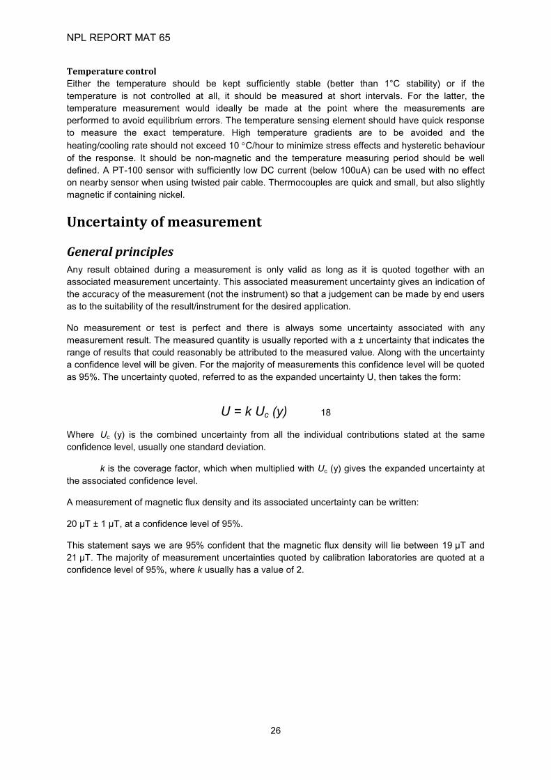
General principles Any result obtained during a measurement is only valid as long as it is quoted together with an associated measurement uncertainty. This associated measurement uncertainty gives an indication of the accuracy of the measurement (not the instrument) so that a judgement can be made by end users as to the suitability of the result/instrument for the desired application.

No measurement or test is perfect and there is always some uncertainty associated with any measurement result. The measured quantity is usually reported with a ± uncertainty that indicates the range of results that could reasonably be attributed to the measured value. Along with the uncertainty a confidence level will be given. For the majority of measurements this confidence level will be quoted as 95%. The uncertainty quoted, referred to as the expanded uncertainty U, then takes the form:

U = k Uc (y) 18

Where Uc (y) is the combined uncertainty from all the individual contributions stated at the same confidence level, usually one standard deviation.

k is the coverage factor, which when multiplied with Uc (y) gives the expanded uncertainty at the associated confidence level.

A measurement of magnetic flux density and its associated uncertainty can be written:

20 µT ± 1 µT, at a confidence level of 95%.

This statement says we are 95% confident that the magnetic flux density will lie between 19 µT and 21 µT. The majority of measurement uncertainties quoted by calibration laboratories are quoted at a confidence level of 95%, where k usually has a value of 2.

NPL REPORT MAT 65

27

Figure 15. Gaussian distribution

It should be noted that statistically there is a 1 in 20 chance that the value could lay outside of this range. Referring to

Figure 15, this is the area of the Gaussian distribution for which the value is more than ± 2σ from the mean. Where higher confidence levels are required further information is given in [11] and [12].

Measurement uncertainties may be made up of many different contributions, some are statistical evaluations that may vary depending upon the device under test, and some contributions are fixed systematic contributions such as uncertainties from calibrated equipment used to conduct the measurement. Traditionally, these were referred to as random and systematic but are now referred to as:

Type A evaluations: uncertainty contributions using statistical analysis, e.g. from repeated measurements.

Type B evaluations: uncertainty contributions from sources such as calibrations certificates, manufacturers specifications, published information and also from common sense and past experience.

Every step of the measurement process and environment should be evaluated to identify the contributions that should be combined to produce the final uncertainty estimate.

The terminology used for reporting measurements can lead to confusion. For example:

• The use of terms such as ‘error’ and ‘uncertainty’ are sometimes incorrectly used interchangeably. The error is the deviation of a result from a true value.

• Specifications are not uncertainties. Specifications give an indication as to the level of performance only.

• Accuracy is not the same as uncertainty. • Tolerances are not uncertainties.

Full and detailed information to assist with the analysis of uncertainties can be found in the ISO Guide to the expression of uncertainty in measurement [11] and UKAS document M3003 [12].

Sources of uncertainty Prior to combining contributions in the uncertainty budget all sources of uncertainty should be assessed. Once assessed they must be quoted in the same units, so that the contributions can be combined at the same level of confidence, usually at a level of one standard deviation, k = 1.

NPL REPORT MAT 65

28

It is not possible to detail all the possible contributions for all circumstances but some general points to be considered are given below:

• Effects of environmental conditions on the measurement process or item under test; • Instrument resolution; • Imperfect realisation of the test procedure; • Measurement repeatability may not be fully representative; • Personal bias in reading instrumentation; • Values of constants used in data evaluation; • Values assigned to measurement standards; • Changes in the characteristics or performance since the last calibration.

Statistical assessment of uncertainties Table 5 shows a typical uncertainty budget used at NPL for the calculation of the uncertainty for the calibration of an instrument measuring magnetic flux densities in the range 90 µT to 350 µT.

Table 5. Typical uncertainty budget.

Calibration of d.c.magnetic flux densities from 90 µT to 350 µT using a fluxgate magnetometer

Source of Uncertainty Reference Value Probability Divisor c1 u1 veff

% Distribution %Calibration of Helmholtz coils Proc. 272 Part 3 0.030 normal 2 1 0.0150 inf

Measurement of voltage across resistor certificate 0.010 rectangular 1.732 1 0.0058 inf.

Value of resistor certificate 0.001 normal 2 1 0.0005 inf.Resolution of fluxgate magnetometer 0.015 rectangular 1.732 1 0.0087 inf.Alignment of probe 0.015 rectangular 1.732 1 0.0087 inf.Repeatability of measurement 0.010 normal 1 1 0.0100 5

Combined uncertainty 0.0226 129Expanded uncertainty for k = 2 0.0451

Uncertainty rounded up to ± 0.05% Shown in Table 5 are the sources of uncertainty and the values associated with that contribution. These contributions should all be as a % or in the same unit such as µT.

The next step is to convert all the values from each source to the same confidence level, usually one standard deviation, or k = 1. For contributions from other equipment calibrations, such as the resistor calibration, the expanded uncertainty quoted on its calibration certificate is entered and the divisor 2 (or whatever k value is quoted on the certificate) applied to obtain the k = 1 value. The two main probability distributions encountered are normal or Gaussian (see

Figure 15) or rectangular. The rectangular distribution is associated with contributions where there is a fixed limit that can be assigned to the value and taken forward into the budget. The probability is that the values will not fall outside of this range, an example of which is instrument resolution.

In the example above the one Type A contribution which has been statistically evaluated is ‘Repeatability of measurement’ and is calculated as the standard error of the mean for each individual set of measurements. Generally, measurements are repeated 3 to 5 times depending upon the parameter/instrument being calibrated. In some circumstances it is not always practical to repeat measurements many times during a calibration. In these circumstances the standard deviation of the measurement system can be obtained from an earlier Type A evaluation. Once the contributions have

NPL REPORT MAT 65

29

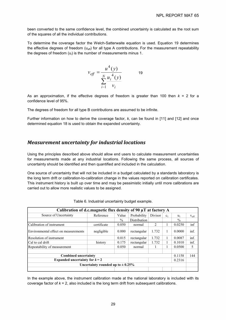
been converted to the same confidence level, the combined uncertainty is calculated as the root sum of the squares of all the individual contributions.

To determine the coverage factor the Welch-Satterwaite equation is used. Equation 19 determines the effective degrees of freedom (υeff) for all type A contributions. For the measurement repeatability the degrees of freedom (υi) is the number of measurements minus 1.

∑−

=N

i i

ieff

vyu

yuv

1

4

4

)()(

19

As an approximation, if the effective degrees of freedom is greater than 100 then k = 2 for a confidence level of 95%.

The degrees of freedom for all type B contributions are assumed to be infinite.

Further information on how to derive the coverage factor, k, can be found in [11] and [12] and once determined equation 18 is used to obtain the expanded uncertainty.

Measurement uncertainty for industrial locations Using the principles described above should allow end users to calculate measurement uncertainties for measurements made at any industrial locations. Following the same process, all sources of uncertainty should be identified and then quantified and included in the calculation.

One source of uncertainty that will not be included in a budget calculated by a standards laboratory is the long term drift or calibration-to-calibration change in the values reported on calibration certificates. This instrument history is built up over time and may be pessimistic initially until more calibrations are carried out to allow more realistic values to be assigned.

Table 6. Industrial uncertainty budget example.

Calibration of d.c.magnetic flux density of 90 µT at factory ASource of Uncertainty Reference Value Probability Divisor c1 u1 veff

% Distribution %Calibration of instrument certificate 0.050 normal 2 1 0.0250 inf

Environmental effect on measurements negligible 0.000 rectangular 1.732 1 0.0000 inf.

Resolution of instrument 0.015 rectangular 1.732 1 0.0087 inf.Cal to cal drift history 0.175 rectangular 1.732 1 0.1010 inf.Repeatability of measurement 0.050 normal 1 1 0.0500 5

Combined uncertainty 0.1158 144Expanded uncertainty for k = 2 0.2316

Uncertainty rounded up to ± 0.25%

In the example above, the instrument calibration made at the national laboratory is included with its coverage factor of k = 2, also included is the long term drift from subsequent calibrations.

NPL REPORT MAT 65

30

Some contributions will be more significant than others. While it may seem unnecessary to include contributions where the values are negligible to the overall value, this can demonstrate to assessors that the contribution has been considered and assessed even if it doesn’t appear to contribute significantly to the overall uncertainty.

Traceability For measurement accuracy to be consistent regardless of the individual, time of measurement or location of measurement, traceability to rigorously maintained measurement standards is required. Traceability requires an unbroken chain of measurements where the primary measurement is usually carried out by the national standards laboratory of the country where the measurements are performed (e.g. NPL in the UK, PTB in Germany). The national standards laboratories are generally, but not exclusively, the pinnacle of each countries measurement pyramid where the lowest measurement uncertainties are offered. The primary standards maintained by the national standards laboratories are then used to calibrate instruments and materials from the next tier of the pyramid, accredited laboratories, which have been accredited to conform to international standard ISO/IEC 17025 [13].

International inter-comparisons

NMI NMI NMI NMI Accredited

laboratories

Industrial &

testing labs.

International comparisons such as [14] as conducted to establish the NMI equivalence.

European capabilities for low magnetic field measurements Information about each national laboratories measurement capabilities in the area of DC magnetic flux density can be found at the BIPM website:

http://www.bipm.org/

Specific information can be found on the ‘Calibration and Measurement Capabilities’ (CMC’s) database:

http://kcdb.bipm.org/AppendixC/default.asp

Using the advanced search drop down menu’s select:

Metrology area: Electricity and Magnetism (EM) Branch: Electric and magnetic fields Service: Electric and magnetic fields Sub-service: Magnetic fields at frequencies below 50 kHz Individual service: DC Magnetic flux density and applied magnetic field strength

NPL REPORT MAT 65

31

Table 7 below gives a brief breakdown of the DC magnetic flux density capabilities of the laboratories taking part in the EMRP 2010 Joint Research Project ‘Metrology for Advanced Industrial Magnetics’ (MetMags).

Table 7. DC Magnetic flux density measurement capabilities

Measurement range BMC (k=2) Method of measurement Czech Republic – CMI 0.05 mT to 100 mT 0.5% Comparison with solenoid 0.02 T to 2 T 0.5% NMR methods Germany – PTB 0.01 mT to 2 mT 20 to 50 nT NMR (free precession) 0.8 mT to 2 mT 2 nT 0.5 mT to 150 mT 0.05 to 6 µT NMR (energy absorption) 100 µT to 150 mT 1 to 10 mT/T Comparison with standard coil 100 µT to 150 mT 0.05 to 10 mT/T Field coils based on NMR Italy – INRIM 15 µT to 500 µT 0.15 to 3 mT/T Helmholtz coils 500 µT to 20 mT 0.15 mT/T 36 mT to 1 T 10 to 25 µT/T NMR United Kingdom - NPL 1 nT to 20 µT 0.15% + 0.5 nT

Fluxgate magnetometers 20 µT to 90 µT 0.003% 90 µT to 350 µT 0.05% 350 µt to 50 mT 0.2% Hall effect magnetometers 50 mT to 8 T 0.0015% NMR

The following countries have entries on the BIPM CMC database for DC Magnetic flux density and applied magnetic field strength.

Table 8

Country NMI Website Australia NMIA http://www.measurement.gov.au/ Bulgaria BIM http://www.damtn.government.bg/index_en.html China NIM http://www.nim.ac.cn/ Czech Republic CMI http://www.cmi.cz/ France LNE http://www.lne.fr/ Germany PTB http://www.ptb.de/ Italy INRIM http://www.inrim.it/ Korea, Republic of KRISS http://www.kriss.re.kr/ Malaysia NML-SIRIM http://www.sirim.my/ Netherlands VSL http://www.vsl.nl/ Poland GUM http://www.gum.gov.pl/pl/strona-glowna/ Russian Federation VNIIFTRI

VNIIM http://www.vniiftri.ru/index.php/ru/ http://www.vniim.ru/

Sweden SP http://www.sp.se/sv/Sidor/default.aspx Switzerland METAS http://www.metas.ch/ Turkey UME http://www.ume.tubitak.gov.tr/ Ukraine NSCIM http://www.metrology.kharkov.ua/ United Kingdom NPL http://www.npl.co.uk/

NPL REPORT MAT 65

32

References [1] J. Lüdke, H. Ahlers, M. Albrecht, Novel Compensated Moment Detection Coil IEEE

Transactions on Magnetics, Volume: 43, Issue: 9, Part: 1.

[2] J. Clarke and A. I. Braginski, ‘The SQUID Handbook Volume 1: Fundamentals and Technology of SQUIDs and SQUID Systems,’ Eds. Weinheim: WILEY-VCH, May 2004.

[3] D. Drung, R. Cantor, M. Peters, H.-J. Scheer, and H. Koch, ‘Low-noise high-speed dc superconducting quantum interference device magnetometer with simplified feedback electronics,’ Appl. Phys. Let., vol. 57, No. 4, pp. 406-408, 23 July 1990.

[4] D. Drung and H. Koch, ‘An integrated DC SQUID magnetometer with variable additional positive feedback,’ Supercond. Sci. Technol. 7 (1994) 242-245.

[5] http://www.magnicon.com/squid-electronics/

[6] http://sine.ni.com/nips/cds/view/p/lang/de/nid/14309

[7] High Performance dc SQUID Electronics XXF-1, Manual, v3.3.8, Magnicon GmbH, 09/2011

[8] A. Schnabel, S. Knappe-Grueneberg, D. Drung, M. Burghoff ,’3-axis measurement of weak dc magnetic fields with SQUID magnetometers, to be published

[9] The Principle of Nuclear Magnetism by A. Abragam. Clarendon Press, ISBN: 978-0198520146.

[10] "The 2006 CODATA Recommended Values of the Fundamental Physical Constants". 7 March 2007. http://physics.nist.gov/cuu/Constants/index.html.

[11] ISO/IEC Guide 98-3:2008 “Guide to the expressions of uncertainty in measurement”.

[12] UKAS document M3003: The Expression of Uncertainty and confidence in Measurement.

[13] ISO/IEC 17025.

[14] K Weyand. Metrologia, 2005, 42, Tech. Suppl., 01006.