BEST PRACTICE IN GRAVITY SURVEYING - Geoscience Australia · BEST PRACTICE IN GRAVITY SURVEYING...

BEST PRACTICE IN GRAVITY SURVEYING

by

Alice S MurrayRay M. Tracey

2

BEST PRACTICE IN GRAVITY SURVEYING

Contents

IntroductionWhat does gravity measure?DefinitionsWhat are we looking for?How can gravity help us?

Gravity SurveyingGravity survey design

Choosing survey parameters for the targetStation selectionCombining different disciplinesAssessment of different platforms

Precision & accuracyWhat can we aim for?What are the constraints?What accuracy do we really need for the job?

EquipmentGravity equipmentPositioning equipment

GPS positioningGravity Survey logistic planning and preparation

Survey numberingPlotting proposed points on the base mapsNative Title clearancesStation sequencingLeapfroggingDesigning a robust network

Marine SurveysTies to land network - no repeat stations

Airborne, satellite and gradiometry measurementsLimitations

Field techniquesCalibrating the metersHow to read the meterKeeping the meters on heatKeep an eye on the readingsLimiting the loop timesUnfavourable conditionsOpen-ended loopsGPS methodsMarking base stationsSite descriptions for bases or terrain corrections

Field logging and pre-processingData loggingProcessing in the field

ProcessingMeter drift

Causes of driftDrift removal

Scale factors and calibrationVariability of scale factorsProcessing of calibration results

3

Post processing and network adjustmentDefinition of the network adjustmentIs the network well conditioned?Processing each meter separatelyChoosing the nodes

Marine and satellite processingEOTVOS correctionsNetwork adjustment - using crossovers

Earth Tide correctionsReason for tidal correctionEAEG tablesThe Longman formulaUncertainties in computationAutomatic correctionsLumping it in with the drift

Gravity anomaliesWhat are gravity anomalies?

Terrain correctionsDefinitionAutomatic corrections - what do we need?What size effect is involved?Some quantitative examples

Error detection and quality controlWhat do errors look like?Automated detection methodsIs it an error or an anomaly?QC checklist

How to rectify errors in a gravity surveyCheck for gravity survey self-consistencyIdentifying tie-points and comparing valuesStatistical comparison and grid differencingIs the coordinate projection compatibleChanging datum, stretching and tilting

The Australian Fundamental Gravity NetworkThe development of the AFGNSite selectionDocumentationCalibration RangesInternational tiesGeodesy

Future DirectionsAbsolute measurementsGradiometryMulti-disciplinary surveys

References

AppendicesA. Standard data interchange format

4

Introduction

What does gravity measure?

Gravity is the force of attraction between masses. In geophysical terms it is the forcedue to the integrated mass of the whole Earth, which acts on the mechanism of ameasuring instrument. Measurements are usually made at the surface of the Earth, inaircraft or on ships. They may also be made in mines or on man-made structures. Thegravity field in space may be inferred from the orbit of a satellite. The measuringinstrument may be a very precise spring balance, a pendulum or a small body fallingin a vacuum.

If the Earth were a perfect homogeneous sphere the gravity field would only dependon the distance from the centre of the Earth. In fact the Earth is a slightly irregularoblate ellipsoid which means that the gravity field at its surface is stronger at thepoles than at the equator. The mass (density) distribution is also uneven, particularlyin the rigid crust, which causes gravity to vary from the expected value as themeasurement position changes. These variations are expressed as gravity anomalies,the mapping of which gives us an insight into the structure of the Earth.

Gravity varies as the inverse square of the distance of the observer from a mass sothat nearby mass variations will have a more pronounced (higher frequency) effectthan more distant masses whose effect will be integrated over a larger area (lowerfrequency). The force is proportional to the mass so that, per unit volume, higherdensity bodies will cause a more positive gravity anomaly than lower density bodies.

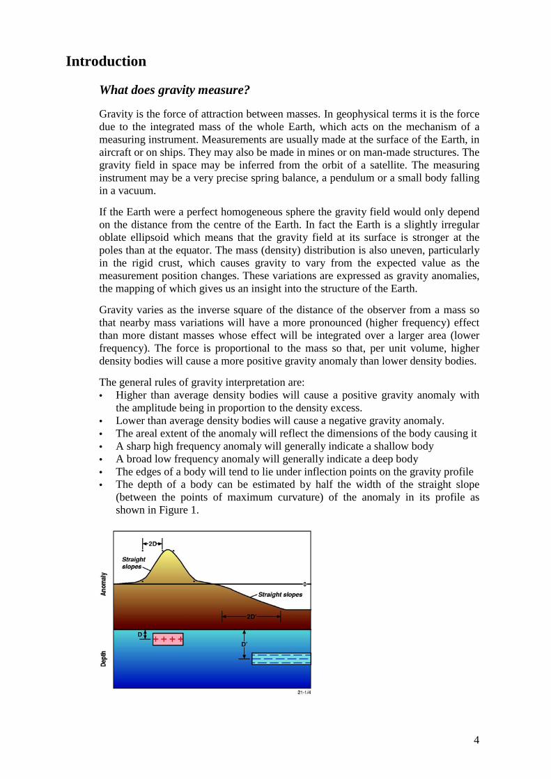
The general rules of gravity interpretation are:• Higher than average density bodies will cause a positive gravity anomaly with

the amplitude being in proportion to the density excess.• Lower than average density bodies will cause a negative gravity anomaly.• The areal extent of the anomaly will reflect the dimensions of the body causing it• A sharp high frequency anomaly will generally indicate a shallow body• A broad low frequency anomaly will generally indicate a deep body• The edges of a body will tend to lie under inflection points on the gravity profile• The depth of a body can be estimated by half the width of the straight slope

(between the points of maximum curvature) of the anomaly in its profile asshown in Figure 1.

5

Definitions

Measurements of gravity are usually expressed in a mass independent term, such asacceleration. The range of gravitational acceleration at the Earth’s surface rangesfrom approximately 9.83 metres per second squared (ms-2) at the poles to 9.77 ms-2 atthe Equator. Gravity variations within countries and particularly within mineralprospects are much smaller and more appropriate units are used. These units are:◊ �� -2) = 10-6 ms-2 (the SI unit)◊ Milligal (mgal) = 10-3cm.s-2 = 10-5 ms-2�� -2 (the traditional cgs unit)◊ �� -2 (the old American measure = 1 meter scale division)◊ �� -8 ms-2 �� -2 (often used for absolute measurements)◊ Newton metre per kilogram (Nm.kg-1) = 1 ms-2 (an alternative form of units)

In this document gravity surveying refers to the field measurement of gravity and theaccompanying measurement of position and elevation; surveying used alone has itscommon meaning of measuring positions and elevations.

What are we looking for?

Gravity operates measurably over the whole range of distances we deal with ingeological interpretations and is not shielded, as may be the case withelectromagnetic fields. The gravity fields of high and low density distributions may,however, interact to mask their individual signatures.

Gravity is just as useful a tool for investigating deep tectonic structures as part ofregional syntheses as it is for finding buried streambeds or caves in urbanengineering studies; it is just that the survey parameters and precision required willbe quite different. In between these extremes we may be interested in outliningsedimentary basins, rifts, faults, dykes or sills, granitic plutons, regolith drainagepatterns or kimberlite pipes. An effective gravity survey can be designed to solvemany of the pertinent physical geological questions. We should first decide what weare looking for, and then design the gravity survey accordingly.

How can gravity help us?

Gravity anomalies only occur when there are density contrasts in the Earth, sogravity surveying is only useful if the structure we are investigating involves bodiesof different density. The density contrast between the bodies must be high enough togive an anomaly that rises above the background noise recorded in the survey. If thedifferences in magnetisation or susceptibility are more characteristic of the bodiesthan density changes then gravity is not the best tool for the job.

The structures we are looking for must vary in density in the direction of themeasurements; a series of flat lying strata of constant thickness will not give anychange in the anomaly at the Earth’s surface. The only deduction we can make is thatthe mean density of the whole suite is more or less than the crustal average based onthe sign of the anomaly. A complicated geological structure at depth may not give asignal at the surface that can be resolved into separate anomalies. In these casesseismic surveys may be more effective.

The size and depth of the bodies we are looking for will determine the optimumobservation spacing for the gravity survey. Sampling theory indicates that the

6

observation spacing should be closer than half the wavelength of the anomaly we areseeking. For shallow bodies an observation spacing equal to the dimension (in themeasurement direction) of the body or twice the dimension for deeper bodies willdetect the existence of a body but not define its shape. Four observations across abody, two just off each edge and two on top of the body (ie spacing about a third ofthe body dimension) will give a reasonable idea of the shape.

The amplitude of the anomaly we are expecting will determine the survey technique�� !� �� "�� -2 anomaly barometer��!�� #��!��$��# ��-2 in��!�� #� ��-2) would notbe effective. The introduction of GPS height determination to better than 0.1 m hasenabled gravity surveying to become effective for regolith modelling.

If the existing gravity coverage in an area is spaced at 11 kilometres and we areinterested in structures of 10 km dimensions we should see some evidence for thesebodies in the existing anomaly pattern. If the anomaly pattern is basically featurelessit indicates that no 10km bodies with significant density contrast are present in thearea. When considering doing a gravity survey it is essential to look at the existingdata and use that in the decision process and survey planning.

The environment may have a bearing on the type of survey that can be done or if onecan be done at all. For example, it may be impossible to do a ground survey in aheavily rainforested area without cutting access lines. The landscape may be sorugged that even though a land survey can be done, the terrain corrections (describedbelow) are the main part of the measured anomalies and accurate calculation of thesecorrections is very difficult. The area may be covered by shifting sand or swamp,making the stabilisation of a meter very difficult, even if you could place one on thesurface. In these areas a lower resolution airborne survey may be the only possibility.

The gravity anomaly pattern is ambiguous in that the same pattern can be producedby an infinite number of structures, however, most of these are physically impossibleor highly unlikely and a skilled interpreter can usually narrow the range of solutionsto a fairly well defined class. Problems can arise when the effect of one body largelycancels out the effect of another body. Subtle high frequency perturbations on theanomaly profile can indicate that this is occurring.

Gravity Surveying

Gravity Survey design

Choosing survey parameters for the targetThe scientific design of gravity surveys can make the difference between a highlysuccessful interpretation tool and a waste of resources. The broad scale surveying ofthe continent with an observation spacing of 11 kilometres could be justified by theneed to define the tectonic structure of the continent and to determine the size andextent of the major tectonic units. Surveys designed to solve geological problemsshould contain sections of various station spacing.

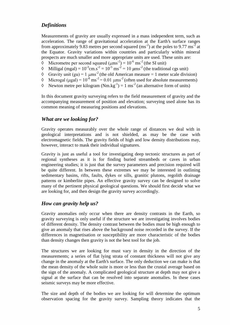
• OrientationDesigning a gravity survey at an angle of about 30/60 degrees to the strike directionof the geology can often provide more information than one oriented at right angles,as illustrated in Figure 2. If a 4km grid runs parallel to a dyke 500m wide it is

7

possible to miss the full effect of the body. If the grid is aligned at 30%�� grid spacing is 2km (4km sin30%�� "�� &�!�� much better defined. If we were looking for small circular features such as kimberlitepipes the station spacing would be critical but not the orientation.

• Density / spacingIn regional surveys, observation density or station spacing is often calculated fromthe area to be covered divided by the number of stations that can be afforded withinthe budget. When planning the station spacing consideration should be given to theexisting anomaly pattern (which areas show high frequency effects and which seemto be smoothly varying) in conjunction with the known geology (where are the densebodies and where are the sedimentary rocks or granites). Using this information and,if available, the aeromagnetic anomalies a series of polygons can be constructed todelimit areas of higher and lower desired station density. In areas of long linearfeatures it is worth considering anisotropic spacing (eg 2 x 1km) with the closerspacing aligned across the features. If no previous or indicative gravity data isavailable an evenly spaced coverage should be surveyed first, followed by targetedin-fill based on the results of this even coverage.

• Regular grid or opportunity (along roads)In most parts of the country a regular grid of observations will necessitate the use ofa helicopter for transport; this will increase the cost by 50 to 100% compared withroad vehicle gravity surveys. In urban areas and farming areas with smallholdingsfairly regular grids of 1, 2 or 4km can be achieved by utilising road transport.

Access may be influenced by the geology, so when conducting gravity surveys onroads it is necessary to check that the roads are not located preferentially along thegeology if that is going to adversely bias the results. For example, roads are oftenpositioned along ridgelines or river valleys for convenience of construction. In somecases this bias is an advantage; such as the greenstone belts of the Eastern Goldfieldsof Western Australia where the land is more fertile on the greenstones and henceroads and sheep or cattle stations tend to be located on them.

• Effectiveness of detailed traversesDetailed traverses provide useful information for interpreting extensive linearfeatures but are of limited use in constructing a reliable gridded surface of an area.When planning a regional gravity survey of an area the coverage should be asregularly spaced as possible in all directions. If, for example, the survey is alongroads spaced at 20km apart, reading stations at less than 5km spacing along the roadsmay not be cost effective. If minimal extra cost is involved closer stations may beread to give greater reliability to the data.

8

Station SelectionThe position of gravity stations should be chosen carefully. The aim is to avoid thereading being influenced by physical effects that are difficult to quantify. Therequirements for stations that need to be re-occupied are described in a later section.

• In rugged countryThe standard formulae for the calculation of simple gravity anomalies assume a flatearth surface at the observation point. Any deviation from a flat surface needs to becompensated by a terrain correction (see below). As terrain corrections are difficultto compute accurately for features near the station it is better to choose a stationposition that minimises this problem (Leaman 1998). If possible the gravity stationshould be sited on a flat area with at least 200m clearance from any sharp change inground elevation.

• What to avoid - moving locationsIn addition to avoidance of large changes in elevation nearby, the gravity station mayneed to be moved from its predesignated location because:◊ Dense vegetation prevents a helicopter landing or would interfere with the GPS◊ Boggy, swampy or snow covered ground prevents access to the site◊ Soft sand, loose rock or mud does not provide a stable footing for the meter◊ The site is exposed to strong winds◊ The site is in a river or lake◊ The site has an important cultural significance◊ Access to the site has not been granted or the site is dangerousWhen the station location needs to be moved it should not be moved more than 10%of the station spacing unless absolutely essential so as to maintain regular coverage..

• City gravity surveysConstructions in cities, towns, airports or mines, for example, can introduce manyterrain effects that are not immediately obvious. Noise and vibration may also be acause of concern in these locations. The following points need to be considered:◊ Measurements near excavations (pits, tunnels, underground car parks) will need

to be corrected for terrain effects◊ Dams, drains, sumps and (underground) tanks that have variable fluid levels

should be avoided.◊ Measurements in or near tall buildings or towers will be affected by terrain and

are susceptible to noise from wind shear. GPS reception may also be poor.◊ Sites near major roads, railways, factories or heavy equipment will be subject to

intermittent vibrationUrban measurements should be made in parks, outside low-rise public buildings or atbenchmarks (for quick position and height control).

Combining different disciplinesBroad scale geophysical surveying is a costly exercise whichever scientific techniqueis being employed. It is sensible to consider employing two or more techniques whenthis can be done at a marginal cost increase over the primary technique and withoutundue compromise to the efficiency and scientific validity of either technique.

• Gravity and geology - competing requirementsJoint gravity and geochemical sampling has been done successfully in WesternAustralia with a reasonably regular 4 km gravity grid being established. Thedemands of the geological sampling may bias the positions to streambeds, outcrops

9

or particular soil types. These positions may also pose terrain effect problems. Thecombined methods can best be accommodated in regional in-fill using 4 or 5 kmstation spacing.

• Gravity bases at geodetic or magnetic sites - synergiesSiting gravity stations at geodetic or magnetic primary reference points has severaladvantages. The total number of sites may be reduced. Measurements can be madeconcurrently thus reducing the operational costs. Deflections of the vertical anddefining of the local slope of the geoid may be important in very precisemeasurements. Precise measurements at exactly the same point over time can becorrelated to define crustal movement.

Assessment of different platformsGravity meters measure gravity acceleration so any other acceleration acting on themeter, such as occurs in a moving platform (aircraft, ship, etc.), will distort themeasurement. If the platform is moving at a constant speed or the instantaneousaccelerations can be calculated, a correction can be applied to the gravity reading togive a meaningful result, however, the value will not be as accurate as ameasurement made on the ground.

• Aircraft - airborne gravity & gradiometry surveys'�� -2 for their work The�� "�#� ��-2. The former figure may reflect the relativeprecision along a flight line but the values are subject to instrument drift and airmovements that cannot be adequately adjusted out by using crossover ties. Airbornereadings are usually filtered by a moving average 5 or 10 point filter so the effectivewavelength is longer than the sample spacing would imply. These methods are quiteexpensive compared with conventional ground readings and do not compete on priceor quality. They are only effective in areas which are very remote, forested, watercovered, swampy or dangerous (pollution, mines or animals). They are ineffective inareas of rugged terrain due to terrain effects and the extreme difficulty in maintaininga perfectly steady flight path.Airborne gradiometry promises to be a much more useful exploration tool. It relieson the simultaneous measurement of gravity at two or more closely separatedlocations. The apparatus is constructed in such a way that nearly all the extraneousforces will cancel out in the comparison of the two (or more) observations and theoutput will be a gravity gradient tensor (gradient vector). The gradients are useful bythemselves as high frequency response sensors of the geology, but for quantitativemodelling a good ground gravity survey of the area is required to provide the groundconstraint.

• Ship - submarineSeaborne gravity surveys are subject to similar stability problems as airborne gravitysurveys but to a lesser degree. The movements of the sea in deep water tend to beslower and more predictable than air currents and a large ship will not be greatlyaffected by chop and swell on a calm day. Obviously gravity surveying in roughweather will give poor results. The elevation of the observation, which is critical incalculating the gravity anomaly, is reasonably well defined for sea surfacemeasurements. Before GPS positioning became the standard the accuracy of marine�� !�� #(�� -2 or worse. New gravity surveys appear to have an�� (# ��-2 which is an order of magnitude less accurate than land gravitysurveys. Submarine gravity surveys are less accurate still and have been only acuriosity. Submarine or sea bottom gravity surveys may be useful in the future for

10

pinpointing high-grade mineral deposits on the sea floor. Underwater gravity metershave been used in shallow water and can give similar accuracy to terrestrial readings.

• Vehicle - car, 4WD, quadbike, motorbikeConventional gravity surveys are often carried out using a wheeled vehicle totransport the operator and equipment between the observation sites. At theobservation site the gravity meter is lifted out of its box or cradle and placed on theground or a base-plate and the meter is levelled and read (optically or digitally)Standard vehicles are used in built up areas or closely settled farmland with goodroads. 4WD vehicles are used on rough tracks, along fence lines or across paddocks,quadbikes (4WD agricultural motorbikes are useful in densely timbered or scrubbyareas where turning ability and vehicle weight are important. Two wheel motorbikesmay be convenient along traverse lines. Care must be taken that gravity meters areprotected from bumps and vibration as much as possible.

• Helicopter - heligravHelicopter transport may be used for conventional gravity surveys where largedistances are travelled between the observation sites and where a regular grid isrequired. They are the most effective (though more expensive) method of transport inremote areas. Heavily forested and very rugged terrain may be problematic.The Scintrex Heligrav system is a self-levelling digital reading gravity meter, withattached tripod, which is suspended by cable from a helicopter. The system iscarefully lowered onto the ground and the helicopter backs off to remove the down-draft from the meter and slacken the cable and then hovers while the reading ismade. The data flows between the helicopter and the meter via an umbilical cordattached to the cable.

Precision & Accuracy

What can we aim for?)��!�� -2 or��*��+��!�� -2. Gravity anomalies,described later, are the most useful representation of the gravity field for interpreters;�� , ��-2.

What are the constraints?The accuracy and effectiveness of gravity surveys depends on several independentvariables as described below. The techniques for measuring these parametersimprove over time and at any stage one or other of the techniques may be thelimiting factor in attaining the ultimate precision.

• PositionsPositions were originally obtained by graphical methods - plotted on topographicmaps or pin pricked on air photos and transferred to base maps. The precision ofthese methods was about 0.1 minute of arc (~200m). Detailed gravity surveys weresurveyed with theodolites and are accurate to about 10 m. Hand held GPS receiverswith selective availability (SA) give positions to 100m and without SA to 7m.Differential GPS can give positions to ±1 cm.

• HeightsHeights for regional gravity surveys were originally measured using aneroidbarometers with accuracy of 10+m, then micro-barometers (5m) and then digitalbarometers (1m). In practice the accuracy achieved depended on the variability of theweather pattern. Detailed gravity survey heights were surveyed using theodolites andstadia to a precision of 0.1m but the accuracy of these measurements could drift by

11

several metres along traverses away from height control. Hand held GPS are notsuitable for heighting but dual frequency receivers with base control can give heightsto a few centimetres. The local model of the geoid must be known to correctgeocentric heights to local elevations or a local correction determined frombenchmarks. The correction (n values) from the geocentric height to the local geoid(AHD) can be found on the Internet. Airborne elevations were measured byaltimeters (pressure gauges) or radar but now GPS receivers are used. Marine waterdepths are measured by sonar.

• GravityGravity surveyors originally used quartz spring meters with a scale range of as little��-�� -2. Measurements could only be made over larger intervals by resettingthe scale range with a coarse reset screw or dial that required precise manualdexterity to achieve any repeatability of readings. Resetting the scale range alsocauses stresses in the mechanism, which relax slowly (over hours or days); this ismanifested by irregular meter drift. The precision of these quartz meters was about�� -2�� !�� -2 or more if a reset hadbeen made. The new electronic quartz meters, such as the Scintrex CG-3, have aworldwide range and incorporate software to compensate for meter tilt and to�� .�� -2.La Coste and Romberg (LC&R) steel spring gravimeters have a worldwide range�� -2. The scale factor varies with dial reading and istabulated by the manufacturer. The drift rate of LC&R meters decreases as they ageand is generally less than the drift of quartz meters.

What accuracy do we really need for the job?The accuracy required of the three components in gravity surveying (gravity value,position and height) is determined by the object of the measurements. Controlstations for one of the components will obviously need to have the greatest accuracyin that component, values for the other components may not even be necessary.Observations for anomaly mapping will generally be dependent on height accuracyfor the overall accuracy.

• Base networkGravity base stations are points where the gravity value is well defined and whichvalue can be used as a reference for gravity surveys being done in that area. TheFundamental Gravity Network (FGN) of base stations is used as the primary gravitycontrol points for Australia. Only the gravity value is necessary at these pointsalthough the position is useful for locating the station and the height may be useful �� )�� # ��-2.Many of the older network stations may have much worse accuracy than this.

• Bases within a general gravity survey/�� -2 and for height to 0.05 metre.

• Reconnaissance coverage'�� "�� 0 "�� -2

�� )�� !��1,�2 ��-2. Much of thehistoric reconnaissance data has height accuracy of only 5 metres.

• In-fill)�� -"�� 2"�� , ��-2 in gravity�� )�� !��1��-2 ��-2.

12

• Mineral prospectThe accuracy of mineral prospect gravity surveys is dictated by the expected�� '�� -2 may be quite significant in the �� )�� !�� # ��-2 and 0.1metre. The gravity values do not have to have FGN control, as relative anomalieswill serve the purpose, however a tie to the FGN will allow the survey to beintegrated into the regional context..• EngineeringEngineering gravity surveys are usually extremely detailed and of limited extent. Theheight precision may be relatively more important than for the mineral prospect case.)�� # ��-2 and 0.05 metre. For some engineering gravitysurveys a gravity value tied to absolute datum is required. Repeated measurements atthe same points over time, to detect crustal movements, need to be of the highestpossible accuracy.

• Detailed traverse - cross-sectionDetailed traverses require a high accuracy relative anomaly for modelling. Relative�� !�� # ��-2, and 0.1 and0.05 metre depending on the station spacing (eg 250 m and 50 m). The absolutevalues are not essential for modelling the traverse in isolation but are necessary whenintegrating the traverse into the regional field. The absolute accuracy is less critical.

Equipment

Gravity EquipmentThere are three main classes of gravity measuring instruments:◊ Pendulums - where the period of the pendulum is inversely proportional to g◊ Sensitive spring balances - where the spring extension is proportional to g◊ Falling bodies timed over a fixed distance of fall in a vacuum tubeWithin each class there are several variants; the types which have been used forgeophysics in Australia are described below. The spring balances are relativeinstruments, which means that they can only be used to measure the difference ingravity between two or more points. Pendulums can be used for relative and absolutemeasurements by calculating the ratio of periods measured at two points or the exactperiod at a particular point. The falling body class measures the absolute gravity.

• PendulumsThe pendulum method of measuring gravity was used all over the world up to themiddle of the 20th Century and was the basis for the 1930 Potsdam Gravity Datum.By the time pendulum measurements were phased out in the 1950s the instrumentshad become quite sophisticated with vacuum chambers, knife edge quartz pivots andprecision chronometers. Mechanical imperfections and wear of the pivot were thelimiting factors in the accuracy of this class of apparatus.

• Quartz spring gravimetersThe technique of crafting a ’zero-length’ spring out of fused quartz lies at the heart ofquartz spring gravimeters. The ’zero-length’ quartz coil (spring), in theory, exerts thesame force regardless of the extension; this implies that the meter has a constantscale factor over the dial range (play of the spring).The extension of the spring must be related to the gravitational force in a predictable,well-behaved way (preferably linear) in order that the meter can be properlycalibrated. The size and play of the quartz springs is limited to ranges between 1400

13

�� 2�� -2 and hence these meters require a mechanical range resetting screw to�� !�� !� � �� #�� -2. Quartz meters firstappeared on the market in the 1930s and were soon generally used for gravitysurveying. The early quartz meters were not thermostatically controlled and tendedto exhibit a diurnal drift curve. Examples of the quartz spring meters are the Worden,Sharpe and Sodin meters. Scintrex have developed an automatic gravimeter CG-3(and higher accuracy variant CG-3M) in which tilt compensation, resetting and driftcorrection is handled electronically; these meters have a worldwide range. Scintrexhas also developed the Heligrav system in which a CG-3 is mounted on a tripod andsuspended from a helicopter by a winch. The meter communicates with the operatorvia an umbilical cord. Manoeuvring the helicopter with the meter dangling below is ahighly skilled and risk-prone operation.

• Steel spring gravimetersLucien LaCoste developed a gravimeter, known as the LaCoste & Romberg (LCR),with a steel mechanism in the 1950s. This meter has a worldwide range and is lessprone to drift than the quartz meters. It is thermostatically controlled to about 50°C.The steel spring has a slowly varying parabolic scale factor which is represented by atable of scale factors for given dial readings. There is some evidence that these scalefactors do vary slightly in a non-linear way with age and depending on the way themeters are transported. There are three main variants of the LCR meters, all of whichare powered by a battery or plugged into a 12 volt power source. The original Gmeter had hand levelling screws, a mechanism locking screw, an eyepice focussingon a graduated scale and a graduated reading dial and revolution counter display.Later G meters were fitted with electronic readout but the nulling feedback was notalways reliable and optical reading still gave the best results. A high precision model,the D meter, was developed in the 1980s. This had a fine and a coarse dial and was�� -2 rather than the eyeball interpolation withthe G meter. The fully electronic E meter was introduced in the 1990s.

• Absolute metersAfter failing to perfect a highly accurate pendulum and with the development oflasers and atomic clocks, researchers in absolute gravimetry turned to the fallingcorner-cube method. The corner cube is raised and dropped in a vacuum chamber.Mirrors on the corner cube reflect laser light at particular points on the cube's fall,the distance is calculated by counting interference fringes The corner cube is thenraised by a mechanical cradle ready for the next drop. A set of 10 drops gives anaverage acceleration value. Several sets may be executed to obtain the desiredaccuracy.There have been various designs for this type of instrument; some prominentexamples are the JILAG, FG5 and A10 'portable' meter.

Positioning equipmentThe dramatic improvement in the accuracy of gravity surveying over the last 20years has been due to the revolution in positioning technology. Positions andparticularly heights had been the limiting factors in calculating accurate gravityanomalies. Positioning for the first reconnaissance gravity surveys was done withoutany equipment, it relied on the observer marking a spot on a map or aerialphotograph. Theodolites were used for positioning the more detailed gravity surveys.

• Pressure based height instrumentsAtmospheric pressure decreases with altitude, so pressure measurements can be usedto calculate elevation. A rough estimate of the pressure decrease is 1 millibar for

14

each 8.7 metre increase in altitude. Theoretically it is possible to calculate anabsolute height above sea level if one assumes a standard atmosphere, howeveratmospheric conditions are constantly changing due to movement of pressuresystems and daily heating cycles (diurnals). Reasonably accurate height differencescan be measured in a local area (within the same pressure regime as the base) if basepressure variations are recorded, the weather pattern is stable and repeat readings aremade at the base and selected field stations during the loop. A detailed description ofthe method is given by Leaman (1984). The height difference network can then betied into the Australian Height Datum at one or more benchmarks. Particularproblems occur if a pressure front travels through the area during a gravity survey asthe base pressure may be out of step with the field pressure during the transit.Pressure measuring apparatus that have been used in gravity surveys are altimeters,precision micro-barometers and digital barometers. The micro-barometers wereusually read in banks of three to improve the height statistics and the digitalbarometers could be directly logged by computers.

• Global positioning system receiversThe introduction of the Global Positioning System (GPS) in the late 1980s enabledgravity to take its place as a precision tool in mapping the fine detail of crustalstructure. The GPS receiver monitors time encoded signals being broadcast by aconstellation of GPS satellites orbiting the Earth, from 3 or more of these signals theposition of the receiver can be calculated in reference to the centre of the Geoid. Theposition values are referred to as the geocentric coordinates. The geocentric geoiddiffers from the local geoid so local coordinates have to be obtained by applying ageoid transformation and/or by tying the network to local spatial control points.

GPS positioning

The NAVSTAR Global Positioning System (GPS) provides a method of determininga position based on measurements to orbiting satellites. It is an all weather systemthat provides position accuracies from tens of metres to millimetres, depending uponthe equipment and configuration used. It can be used anywhere on the globe, 24hours of the day and with no user charge.GPS technology is used extensively in gravity surveying these days where it hasgreatly reduced the cost of providing accurate positions and heights. In particular, forsurveys where the error in station height is required to be less than 10cm, GPS isconsiderably cheaper than other methods such as optical levelling.The basic theory and operation of GPS is described in texts such as Hoffman-Wellenhof et al, 1994 or Leick, 1995. Commercial GPS receivers can be singlefrequency or dual frequency. The accuracy of a position obtained with a singlefrequency receiver is about 7m horizontal and 12m vertical compared with about 5mhorizontal and 8m vertical accuracy for a dual frequency receiver. These accuraciesare possible since Selective Availability, a deliberate degradation of the GPSpositions, was turned off on 1 May 2000.Clearly this vertical accuracy is not sufficient for gravity surveying but it can beimproved by employing differential or relative techniques using two or morereceivers. In the simplest case of differential GPS, one receiver is set up over aknown point, the base, while another receiver, the rover, occupies unknown points.The corrections that need to be applied to the GPS position for the base to obtain itstrue position are also applied to the GPS position obtained at the same time by therover at an unknown point. These corrections can be applied in near real-time byutilising a data link, such as radio-modems, to transmit the corrections to the rovingreceiver or they can be applied during post-processing of the recorded data from both

15

receivers. This form of differential GPS, or DGPS, can be employed using bothsingle and dual frequency receivers. The differential corrections can be obtained byusing your own receiver or can be obtained from a variety of commercial systemsthat make the corrections available either in real-time or for post-processing. Theaccuracy of this form of differential GPS can approach sub-metre horizontal andnear-metre vertical depending on the quality of receiver used, whether it is single ordual frequency, and the type of corrections applied. The vertical accuracy obtainedwith these systems, at least one metre, would introduce an error of about 3 µms-2 inthe gravity value. Clearly the vertical accuracy obtained with this type of differentialGPS is not sufficient for most gravity surveys.Carrier-phase differential GPS provides the highest accuracy and is best suited forgravity surveying. This technique uses the phase differences in the carrier wave ofthe signals transmitted from the GPS satellites that are received simultaneously at therover and the base to compute a position for the rover relative to the base. Sub-centimetre accuracy in horizontal and vertical position is achievable using thismethod of differential GPS. Carrier-phase differential GPS can be either post-processed or computed in real-time. The distance between the base and rovingreceivers is limited in carrier-phase DGPS owing to differences in the effect of theionosphere on the satellite signals received at the base and the rover if they are toodistant. This distance, known as the baseline, is generally limited to about 20km. Thebaseline distance may be extended to up to 80km or more in situations where there isno interruption in the satellite signals received by the rover, such as when the rovingreceiver is installed in a helicopter.The level of accuracy required in the determination of gravity station positions isdependent to a large degree on the type of gravity survey and the size of theanomalies that are expected to be detected. An error of 10cm in the height of astation would result in an error of about 0.3 µms-2. Errors of this magnitude areacceptable in regional gravity surveys with station spacings in the order of one ormore kilometres, however for more detailed surveys the height of the gravity stationneeds to be determined more accurately. To obtain these greater accuracies, shorterbaselines and a more rigorous approach to minimising errors needs to be employed.This more rigorous method increases the cost of the survey by increasing the numberof GPS base stations needed and the number of measurements required.The accuracy of the horizontal position of a gravity station is much less critical withlatitude errors producing the most effect. An error of 100 metres in the north-southposition will result in about 0.5 µms-2 error in the gravity value.

Gravity survey logistic planning and preparation

Survey numberingMost survey numbering schemes involve the year, or last two digits of the year, inthe survey number as a quick and easily recognisable guide to the age of the survey.The original AGSO numbering scheme, developed in the late 1950s, was a four digitnumber with the last two digits of the year as the first two digits of the surveynumber. The last two digits of the survey number originally signified the type ofsurvey according to the following rules:

00-29: surveys done by or for AGSO/BMR (00 sometimes for control work)30-89: surveys done by other organisations (state governments, private

companies, universities or international bodies). At some times certainnumbers were reserved for particular states (eg 50-59 for Tasmania) orfor marine surveys (60-89), but no consistent pattern was set.

90-98: control surveys for the Fundamental Gravity Network99: absolute gravity measurements

16

In the late 1980s the numbering system was changed to indicate the state as follows:00-19: AGSO or national surveys20-29: New South Wales30-39 Victoria40-49: Queensland50-59: South Australia60-69: Western Australia70-79: Tasmania80-89: Northern Territory90-99: Base and absolute stations as above

Within each state series the government surveys are numbered 0,1,2,etc. and theprivate company surveys as 9,8,7,etc. If more than ten surveys are done in a state inone year, general numbers from 00-19 may be used. Related small surveys should begiven the same number, as should surveys carrying over from one year to the next.The new AGSO survey numbers, for year 2000 and onwards, are six digits with thefirst four being the year of commencement of the survey. All the old surveys havehad 19 added as a prefix to bring them into line with the new scheme.

Plotting proposed points on the base mapsIt is good practice to plot the proposed observation locations on a topographic mapbefore starting the gravity survey. Areas of difficult terrain and cultural features willrequire the re-positioning of some stations. Private landholders may need to beinformed and permission sought for working on their property.

Native title clearancesA large part of Australia is now under Native Title or has been claimed. It isnecessary to negotiate access to the land with the leaders of the community. Maps ofthe proposed station locations will be necessary to help identify areas of exclusionand sacred sites. Negotiation with the titleholders normally takes several months andthis time should be allowed for in planning the gravity survey.

Station sequencingThe order in which stations are read may have a significant effect on the cost oftransport for the gravity survey and the efficiency of operation. Keeping the timetaken for each loop and the distance travelled to a minimum also reduces the risk oferror propagation and the loss of data through equipment problems. The position ofrepeat and tie stations in each loop has a bearing on the strength of the network; forbest results these stations should be evenly spaced in the reading order of the loop.

LeapfroggingIn difficult terrain, areas of limited access, or when transport is limited it may beimpracticable to control loops from a single base station. One crew may startworking from a base station, travel out to the limit of baseline reliability and set up anew base. The old base crew then travels past the new base crew and works untilthey set up a further base. This leapfrogging procedure continues until a loop closurecan be achieved. With limited transport, two crews may set out from base on thehelicopter or vehicle, one crew is dropped off at the first station and the second crewis carried to and dropped off at the second station. The transport then returns to thefirst station and transports the first crew to the third station, then the second crew tothe fourth station and so on. This method of leapfrogging is particularly efficientwhen each crew needs to spend a significant length of time at each station, as forexample in a joint geochemical and gravity survey.

Designing a robust networkA gravity survey network is a series of interlocking closed loops of gravityobservations. A robust network will generally allow two or more independent paths

17

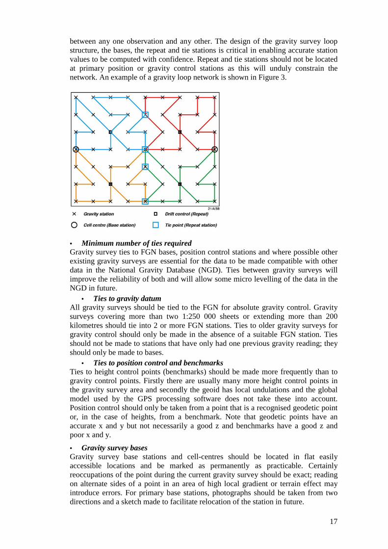
between any one observation and any other. The design of the gravity survey loopstructure, the bases, the repeat and tie stations is critical in enabling accurate stationvalues to be computed with confidence. Repeat and tie stations should not be locatedat primary position or gravity control stations as this will unduly constrain thenetwork. An example of a gravity loop network is shown in Figure 3.

• Minimum number of ties requiredGravity survey ties to FGN bases, position control stations and where possible otherexisting gravity surveys are essential for the data to be made compatible with otherdata in the National Gravity Database (NGD). Ties between gravity surveys willimprove the reliability of both and will allow some micro levelling of the data in theNGD in future.

• Ties to gravity datumAll gravity surveys should be tied to the FGN for absolute gravity control. Gravitysurveys covering more than two 1:250 000 sheets or extending more than 200kilometres should tie into 2 or more FGN stations. Ties to older gravity surveys forgravity control should only be made in the absence of a suitable FGN station. Tiesshould not be made to stations that have only had one previous gravity reading; theyshould only be made to bases.

• Ties to position control and benchmarksTies to height control points (benchmarks) should be made more frequently than togravity control points. Firstly there are usually many more height control points inthe gravity survey area and secondly the geoid has local undulations and the globalmodel used by the GPS processing software does not take these into account.Position control should only be taken from a point that is a recognised geodetic pointor, in the case of heights, from a benchmark. Note that geodetic points have anaccurate x and y but not necessarily a good z and benchmarks have a good z andpoor x and y.

• Gravity survey basesGravity survey base stations and cell-centres should be located in flat easilyaccessible locations and be marked as permanently as practicable. Certainlyreoccupations of the point during the current gravity survey should be exact; readingon alternate sides of a point in an area of high local gradient or terrain effect mayintroduce errors. For primary base stations, photographs should be taken from twodirections and a sketch made to facilitate relocation of the station in future.

18

• Control points should not be cell centresAs mentioned above, cell-centres and other repeat stations should not be located atposition or gravity control points. A control point may be used for the primary basestation of the gravity survey but this point should not be used as a cell centre as thiswould have the effect of splitting the network in the matrix inversion process, asdescribed later. The cell centre may be an arbitrary distance from the control pointand must have a different station number. For the same reason ties between loopsshould not be made at control points. To derive reliable statistics about a gravitysurvey the network nodes should be as freely adjustable as possible.• Repeat and tie stationsWith gravity surveying where each observation is a sample of a physical parameterthat is subject to errors from various sources (human or equipment), the more repeatsto verify the data, the better. Operationally, however, the less repeats the quicker thegravity survey can be completed. A balance must be struck between achievingreliable results and keeping the cost per new station affordable.Repeat stations are stations where a reading is made two or more times within theloop, but not as consecutive readings. Tie stations are stations read in two or moreloops or two or more gravity surveys. Repeat stations are used to check equipmentand processing performance and usually do not play a part in the networkadjustment.In a loop of 23 stations there should be two repeat or tie stations in addition to thecell-centre. For a standard cloverleaf pattern of four loops radiating from a cellcentre, if each has 23 stations and the cell-centre is common, there are 89 distinctstations. If there are two repeats or ties in each loop and one cell-centre there will benine repeats; which is close to 10% of the total

• As an insurance against equipment failuresMany problems can arise during a gravity survey but sound survey design can helpto minimise the effects. Problems may be due to equipment; battery failure, transportproblems or faulty data logging; or external sources; earthquakes or lack of satellites.When a problem does occur it usually means the loss of the most recently measureddata. Data loss can be kept to a minimum by designing repeat or tie stations no morethan ten stations apart, data loss is then limited to the stations after the last repeatstation.

Marine gravity surveys

Ties to land network - no repeat stationsThere are no ties or repeat stations in a marine gravity survey as it is practicallyimpossible to reposition a ship exactly and the tide level would be different anyway.Marine gravity surveys have to be tied to the absolute datum by using a portable landgravimeter to measure the interval between the ship-borne meter and an FGN orknown gravity base station at the port of call. Often the ship traverse will not be aclosed loop and the control will be two different bases, one at each end. Standardnetwork adjustment does not work in these cases and interpolation or error spreadingmust be used.Many marine gravity surveys are designed with crossover lines so an interpolated tieor repeat value can be calculated and used for network adjustment.

Airborne, satellite and gradiometry measurementsLimitationsDirect control of airborne gravity surveys is even more difficult than marine gravitysurveys. The best solution is good ground gravity control in strategic places so thatan upward continuation to the flying height can be used to check the airborne data.

19

Ground control is even more important for gradiometry surveys. Conventionalgravity survey interpretation can be ambiguous and gradiometry is even moreobscure. Using the ground survey as a quantitative constraint, the qualitative value ofthe gradiometry can be fully exploited.

Field Technique

Calibrating the metersAll spring type gravity meters have a scale factor. Quartz meters have a ’constant’scale factor that is often marked on the top of the meter. LCR meters come with amaker’s table of scale factors versus dial readings. Scale factors tend to vary slightlyas the meter ages, they may also be changed if the meter is overhauled or rebuilt. Thescale factor will also change if the level adjustment is off centre, the sensitivity hasbeen adjusted, the vacuum is not tight enough or the thermostat is not workingproperly. There is also evidence of non-linear effects, which have been documented(Murray, 1995), when several meters are used to measure the same differencesbetween points. For all the above reasons it is recommended that all gravity metersare calibrated before and after each gravity survey. Calibration involves reading themeter at two points of known gravity; the gravity interval between them should be at�� #�� -2. LCR meters should also be calibrated, even though they have avariable scale factor, as this will detect deviations from the maker’s table and help tostatistically define each meter’s behaviour. Inconsistent calibration results are a goodindicator of a faulty meter.Descriptions and values of suitable calibration points are available from AGSO.

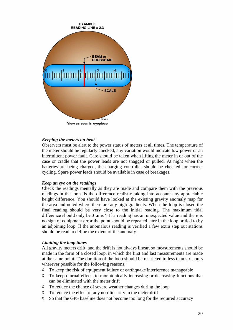
How to read the meterThe secret of consistent and accurate meter reading is following a routine. If thesame procedure is followed for each reading the sources of difference are reducedSome tips for a good reading technique with optical meters are:◊ Level the meter before unclamping◊ Do not turn the dial while the meter is clamped◊ Be familiar with the reading line on the graticule and where the beam should be

placed as shown in Figure 4 (eg just touching the left of the line)◊ Always turn the dial in the same direction when approaching the reading line -

you may need to wind the dial back past the reading line to do this◊ Always use the same eye for readingFor electronic meters, keep the recording time the same for each reading

20

Keeping the meters on heatObservers must be alert to the power status of meters at all times. The temperature ofthe meter should be regularly checked, any variation would indicate low power or anintermittent power fault. Care should be taken when lifting the meter in or out of thecase or cradle that the power leads are not snagged or pulled. At night when thebatteries are being charged, the charging controller should be checked for correctcycling. Spare power leads should be available in case of breakages.

Keep an eye on the readingsCheck the readings mentally as they are made and compare them with the previousreadings in the loop. Is the difference realistic taking into account any appreciableheight difference. You should have looked at the existing gravity anomaly map forthe area and noted where there are any high gradients. When the loop is closed thefinal reading should be very close to the initial reading. The maximum tidal � �� , ��-2. If a reading has an unexpected value and there isno sign of equipment error the point should be repeated later in the loop or tied to byan adjoining loop. If the anomalous reading is verified a few extra step out stationsshould be read to define the extent of the anomaly.

Limiting the loop timesAll gravity meters drift, and the drift is not always linear, so measurements should bemade in the form of a closed loop, in which the first and last measurements are madeat the same point. The duration of the loop should be restricted to less than six hourswherever possible for the following reasons:◊ To keep the risk of equipment failure or earthquake interference manageable◊ To keep diurnal effects to monotonically increasing or decreasing functions that

can be eliminated with the meter drift◊ To reduce the chance of severe weather changes during the loop◊ To reduce the effect of any non-linearity in the meter drift◊ So that the GPS baseline does not become too long for the required accuracy

21

Unfavourable conditionsGravity surveying can be adversely affected by environmental or cultural conditionsat individual station sites or applying to the whole gravity survey. The remedy forthese problems is to wait for them to abate or to move the station to a better site. Inparticular, base stations should not be placed in exposed or noisy positions.

• Earthquake noiseGravity meters are extremely sensitive instruments, they can be affected by largeearthquakes anywhere in the world. The effect is manifested by an unstable reading,which tends to oscillate with a period of a few seconds. The beam on an opticallyread meter will swing from side to side on the scale, the amount of movement willdepend on the sensitivity of the meter. On some less sensitive meters the mid-pointof the oscillation can be accurately judged and a reading recorded. Electronic metersmay show an increased error value and take longer to stabilise.The intensity and duration of the earthquake effect will depend on the geology of thearea, with the greatest effect being on a poorly consolidated sedimentary basin andleast effect on cratonic outcrop. Large earthquakes in distant parts can causedisruption to readings over many hours, whereas small local earthquakes have only afew minutes effect.

• Windy or stormy weatherGravity meters buffeted by the wind will give noisy readings and barometric heightswill be distorted by large pressure changes in storms. Close to coastlines groundnoise may be generated by large long period waves. Bad weather can also distract theobserver making the likelihood of errors greater.

• Ambient temperature too highThermostat controls on gravity meters are usually set at about 50°C, obviously if theambient temperature rises above this the meter temperature may fluctuate, causingerrors in the readings. The meter is usually read just above the ground where radiatedheat may drive the temperature well above the prevailing air temperature. If themeter is exposed to direct sunlight the, usually black, top plate will heat up andadversely affect level bubbles and cause temperature gradients inside the meter.Meters transported in vehicles without air-conditioning may also be exposed toexcessive temperatures. As far as possible meters should not be subject totemperature shocks, for example, taking the meter from an air-conditioned vehicle toa high external temperature.

• Unstable footingsCare must be taken when placing a gravimeter on unstable ground as the meter maymove off level during the measurement. Examples of unstable ground are mud, sand,shale, scree, floating ice, salt crust and loose pavement. The meter base-plate mayneed to be pushed in until the bottom of the flat plate is resting on the surface. Alarge board may be placed on mud, sand or salt crust to give stability to the meter.The operator should be careful not to dislodge the meter when kneeling or walkingbeside it.

• Cultural artefactsSome parts of Australia are under Native Title and negotiation is necessary with thetitle-holders to gain access to the land under their control. There will probably besome places on this land which are sacred sites or restricted areas and the positionsof stations and travel routes will need to be moved to avoid them.

22

War memorials and churches are often good stable and permanent sites for gravitybase stations but sensitivity should be shown and permission sought when apermanent mark is to be placed on the site.

Open-ended loopsAll gravity loops should be closed for normal land gravity surveys. Closing a loopmeans reading the gravimeter at the same place at the beginning and end of the loop.The only way reliable results can be obtained from a loop that is not closed is whenthe first and last points read are well-defined base stations. Examples of open loopsare ship traverses across an ocean or around a coastline, which start at one port andend at another. Another non-conventional loop structure is the ladder sequence, suchas A-B-A-B-C-B-C-D-C-D-etc. Although this sequence starts and finishes atdifferent points it can be seen that the series is made up of intersecting closed loops.

• Recovering from disastersSometimes a gravity loop can not be completed as planned. This may be due to avehicle breakdown, bad weather or equipment failure. In this case the last readstation should be clearly marked for a follow-up tie. If the last point read in theincomplete loop can not be exactly located the next last should be located and so onuntil a sure relocation is made. All stations read in the original loop after the surerelocation will be lost. A follow-up tie should be made by reading at this relocatedpoint, then at the original base of the loop and then back at the relocated point ifpossible, or a tie from base to relocated point to base.

GPS methodsThe most common field method used when GPS surveying for gravity surveys iscalled kinematic surveying. In this method data is recorded continuously by both thebase and roving receivers during the gravity loop. In the early days of kinematicsurvey it was necessary to start recording by occupying a known baseline to initialisethe system. This is no longer necessary, due to advances in receiver technology anddata processing algorithms and techniques. The kinematic method produces atrajectory of the GPS antenna’s position for the duration of recording. The data canbe post-processed or precise positions can be obtained in real-time using a data link.

Real-time kinematic, known as RTK, saves time as there is no need to post-processthe data, however it is limited in its use by the reliability of the data link. Most RTKsystems use UHF radio modems as the data link between the base and rovingreceivers. These systems can not be used in rough terrain or over long distanceswithout the use of radio repeaters because the UHF link is generally limited to line ofsight operation. Satellite telephones and cellular telephones have been usedsuccessfully for RTK surveying where UHF is not suitable, but this is a costlyalternative.

Marking base stationsGravity loop and network adjustment depends on exact reoccupation of a readingstation at a repeat, tie or loop-base station. These points are nodes in the adjustmentnetwork and any mis-location and consequent differential in gravity value will bepropagated through the network, thus reducing its accuracy. The required type andpermanence of station marking depends upon the significance of the station in thegravity survey and its use or future use.

• Repeat stations are those that are read twice or more within the loop and not inany other loop; a colour tape or spray of paint will suffice for these. This markonly needs to survive for the duration of the loop.

23

• Tie stations are those read in more than one loop, the permanence needed willdepend on the likely time between returns. The time span may be several months.A short stake with colour tape and a station number label should suffice.

• Loop-base stations or cell centres are the start and end point of loops. Usuallythese points will be used for a number of loops. Exact reoccupation is veryimportant at these points and a flat stable surface is recommended. The readingpoint should be marked with paint and a star picket with labelled tape or tagshould be driven into the ground beside (within 0.5 m) the reading point.

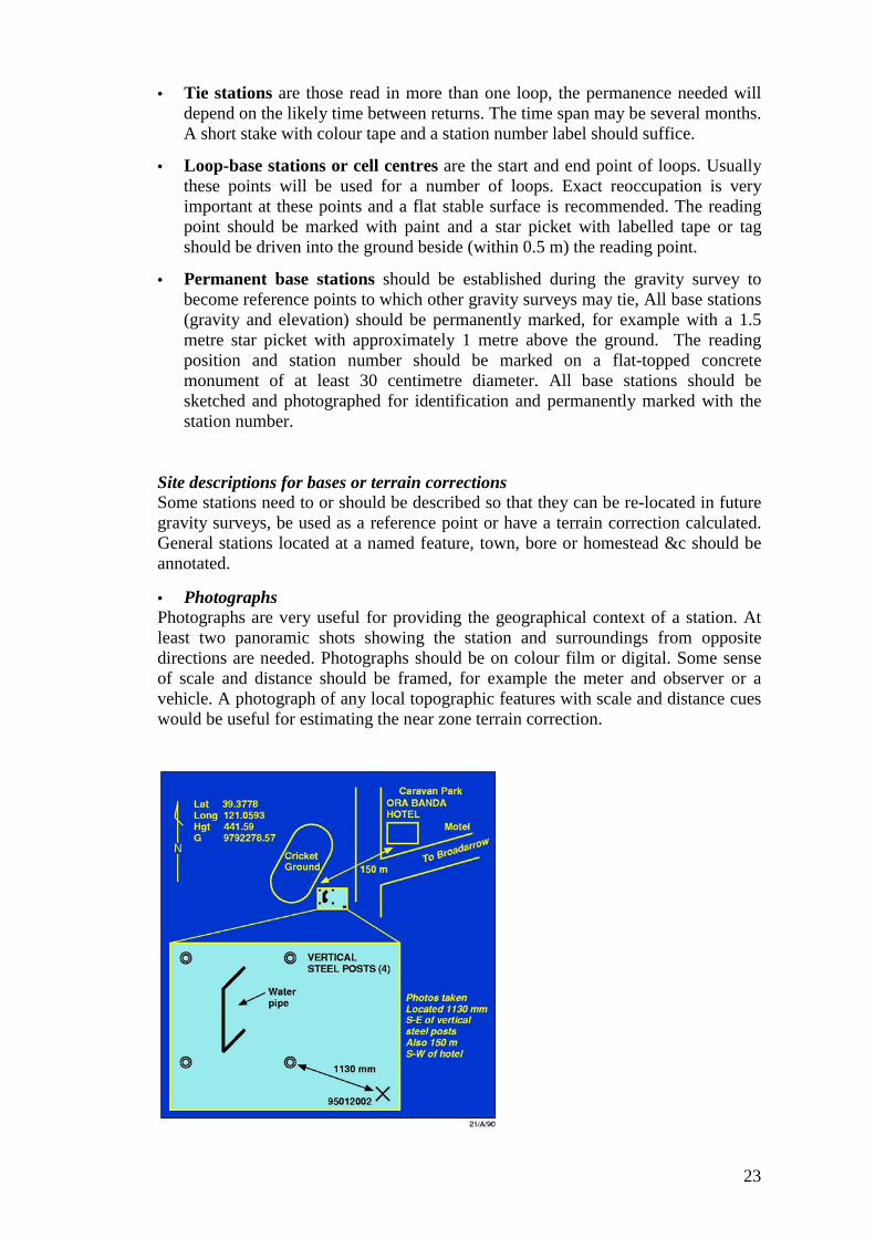
• Permanent base stations should be established during the gravity survey tobecome reference points to which other gravity surveys may tie, All base stations(gravity and elevation) should be permanently marked, for example with a 1.5metre star picket with approximately 1 metre above the ground. The readingposition and station number should be marked on a flat-topped concretemonument of at least 30 centimetre diameter. All base stations should besketched and photographed for identification and permanently marked with thestation number.

Site descriptions for bases or terrain correctionsSome stations need to or should be described so that they can be re-located in futuregravity surveys, be used as a reference point or have a terrain correction calculated.General stations located at a named feature, town, bore or homestead &c should beannotated.

• PhotographsPhotographs are very useful for providing the geographical context of a station. Atleast two panoramic shots showing the station and surroundings from oppositedirections are needed. Photographs should be on colour film or digital. Some senseof scale and distance should be framed, for example the meter and observer or avehicle. A photograph of any local topographic features with scale and distance cueswould be useful for estimating the near zone terrain correction.

24

• Sketch mapDiagrams, as illustrated in Figure 5, are useful for the precise location of theobservation site, particularly in relation to a building or cultural structure. Exactdistances and angles can be annotated and, if necessary, a side elevation can bedrawn. Sketch maps of the surrounding area and the district may be included to makethe re-location of the station easier. Sketch maps are always made for FGN stations.

• What is needed for estimating terrain correctionsIn order to calculate the near zone effect of terrain corrections an approximate modelof mass distributions around the station needs to be created. Distances, bearings andelevations need to be estimated for any topographic variation from a flat plain at theelevation of the observation point. If the observation point is on sloping ground theslope and the extent of the sloping ground needs to be estimated. Note that hills andvalleys do not cancel each other out in the calculations.

• Identifying marks/features, serial numbers of old pointsAll stations read on the site of an existing station should be annotated with the nameor number of the existing station. Stations located at a named place, in a town, at apoint which has a number (benchmark or geodetic station) or at a road junction, forexample, should have these details annotated in the description.

Field logging and pre-processing

Data loggingRecording of gravity survey readings up to the 1980s was done manually in fieldnotebooks. Some of these notebooks were designed for data entry to mainframecomputer processing and had the fields and columns delimited, but many gravitysurveys were recorded free hand. There was always the risk of transcription errors ordyslexia between the dial reading, notebook and keyboard.Hand held computers and data loggers were introduced in the 1980s. The moresophisticated systems had a basic capacity for prompting and data validation.In the 1990s digitally recording equipment with direct data logging to disc orcomputer became the standard.

Processing in the field - checking, verification, instant follow-upDaily processing of each day’s data is very important to check that equipment isfunctioning normally, satellite lock is maintained, the meter drift is reasonable, andthe station readings are sensible. If real time position values have been recordedthese can be used for the daily checking. Simple gravity anomalies should becalculated and plotted on a map or imaged to build up a progressive picture of thesurvey results. Unexpected anomalies should be checked for gravity, position orheight irregularity and any obvious errors flagged for re-measurement the next day.If the station values are plausible the station should be re-read, and if unchangedseveral step-out stations should be read to scope the anomaly.

Processing

Meter drift

Causes of driftAll gravity meters drift. Meter drift is caused by mechanical stresses and stains in themechanism as the meter is moved, subjected to vibration, knocked, unclamped, reset,subjected to heat stresses or has the dial turned etc, Meter drift does tend to moderate

25

with age as the mechanism creeps to a lower stress level. Meter drift is effectively atemporary and variable change in scale factor.

Drift removalRemoval of meter drift plays a significant part in the accuracy of gravity surveys.Meter drift can only be sampled at points of known gravity or at repeated stationsthat only account for about 10% of readings in a normal gravity survey. In betweenthese sample points we have to make assumptions about how the drift behaves.

• Piecewise linear driftThe simplest assumption is that drift is linear and, in the absence of documented driftbehaviour of each meter, this is probably the logical thing to do. This assumption isthe basis of the piecewise linear method of drift removal.

• Long term driftThe long-term drift of a meter can be documented by recording the readings atrepeated base stations over a number of weeks or months. From these readings, along-term drift curve can be constructed. The long-term drift curve is of limited usein modelling the drift performance of a meter over the time scale of a gravity loopbut may be useful for ties that take several days to complete.

• Drift curves from experienceThe short-term drift performance of meters should be tested more regularly. It isworthwhile running meters over a series of known base stations under operationalconditions to see how the meter drift performs. If this is done regularly, acharacteristic drift curve may be developed and applied to real gravity survey results.

• Automatic drift removalSome electronic gravimeters, such as the Scintrex CG-3, have in-built automatic driftremoval based on linear drift between loop-base station readings. It is important tocheck from time to time that the automatic drift correction is working properly, byreading at points with a known or previously read value between the loop-basestation readings. Many processing programs will apply a linear drift correction to theloops before network adjustment.

• TaresGravimeters are prone to have steps in their drift curves. Some mechanical hitch orstick catches or releases and causes the subsequent readings to be higher or lower�� )��3�� -2 in magnitude. Itis often difficult to determine where in the loop a tare has occurred unless it is largeenough to be obvious. Tares are detected by the difference in reading at base stationsor repeat points being much more than expected from normal drift. If a tare occurs ina loop it should be isolated to a segment between two repeated points and thatsegment will have to be re-measured. The before and after parts of the loop mayneed to be separated for processing.

• Resetting the rangeResetting the range on older quartz instruments is an imprecise process and is likelyto radically change the drift characteristics for some time after the change. Reliableresults will not be achieved if a meter is reset while measuring a loop. A reset couldbe considered to be a large tare.

• Bumps and bangsGravimeters are delicate instruments that can be adversely affected by roughhandling. Sudden accelerations may cause tares or changes to the drift behaviour. Ameter should be thoroughly checked and re-calibrated after a serious shock such asbeing knocked over.

26

• Travel sicknessProlonged or rough travel may change the drift behaviour of a meter. There is someevidence that meters transported by helicopter exhibit different drift behaviour fromthose transported by road or on foot.

• Morning sicknessFor the first few readings each morning a gravimeter often appears to have anelevated drift. This may be due to prolonged inactivity during the night. There isoften a saw-tooth pattern when the readings at a base station, that is read over severaldays, are plotted. Making one or two dummy readings at the base camp, beforestarting to make measurements from the loop-base, may alleviate this effect.

Scale factors and calibration

Variability of scale factorsAll gravimeters come from the manufacturer with a scale factor or table of factors.However this (these) factor(s) may change over time as the meter becomes worn andthe stresses in the materials dissipate. Quartz meters, with a single calibration factor,can be calibrated before and after a gravity survey and the average calibration factorused in the processing of the data. LCR meters, with varying scale factor, should becalibrated between points of known value across a wide range of the dial to detectany variation from the maker’s table.

• Variation over timeA table of scale factors versus time should be established so that the appropriatefactor can be chosen when reprocessing a gravity survey. For LCR meters a scalefactor adjustment factor may be stored. Scale factors may change significantly if themeter is overhauled or upgraded and new sets of factors and dates need to be stored.

• Variation with readingIt is possible that the LCR scale factor adjustment factor is also a function of the dialreading which would require a non-linear adjustment to the non-linear scale factor. Asimilar problem with the quartz meters is less likely if they are calibrated properly.

Processing of calibration resultsCalibration results should be processed before the gravity survey begins to check forany gross difference from the expected value, which could indicate a malfunction inthe meter. The average of the pre- and post-survey calibration results can be used todefine the scale factor to be used in reducing the gravity survey data.

Post processing and network adjustment

Definition of the network adjustmentThe gravity survey network is the set of interconnected loops and the attachedcontrol stations. When the scale factor has been determined and the Earth tidecorrection and meter drift have been removed from the readings in a loop asdescribed above, we are left with a series of gravity differences at each stationrelative to the loop-base. These differences need to be adjusted to fit any controlstations or tie points in the loop. The repeat points may have been adjusted to thesame value as part of the drift removal but may be left as measured and adjustedhere. The network adjustment is the process of fitting the loops together and usingthe control points as the datum level. In a simple network where one control valuecan be propagated throughout, loop by loop, there is no ambiguity in the values. Inthe case of two or more control values and loops which interconnect each other via

27

different paths a more complex adjustment is required. Commonly, a least squareadjustment solution is obtained via a matrix inversion.

Is the network well conditioned?For a network to be well conditioned all loops must be connected together and theconnection point must not be a control station. Adjustments can not be propagatedthrough a control station so a set of non-intersecting loops, which are only connectedat a control station, is a fragmented network. Incorrect station identification may alsocause a fragmented network.

Processing each meter separatelyResults from each meter should initially be processed separately to check that themeter performance is satisfactory. Comparing the tie point values between the metersmay also show systematic variations indicating the need for scale factor adjustment.Errors that are detected should be corrected or deleted at this stage.

Choosing the nodesA node in the network is a tie-point or base station whose several measurements willbe adjusted to a single value in the network adjustment. The choice of nodesdetermines how adjustments are spread through the network. At a minimum theloop-bases and tie points must be specified as free nodes and at least one controlpoint must be specified as a fixed node. Every point that has more than one readingmay be specified as a node and every point that has an external value can be used asa fixed node.

• Minimal constraint solutionAn adjustment should be made using one control point and the minimum number ofnodes needed to link the network. This adjustment will show the internal consistencyof the data and highlight station number errors and mis-occupations. Adjustmentswill be distributed throughout the network with minimal constraint

• Using control values to isolate the errorsAdding more than one control value to the adjustment will introduce constraints onthe node adjustments. This will tend to isolate problem areas. Errors in the meterscale factors will be indicated by an increase in the error statistics compared with thesingle meter adjustments.

Marine and satellite processing

EOTVOS correctionsThese corrections are applied to compensate for changes in heading and velocity(change in angular momentum).

Network adjustment - using crossoversNetwork adjustment for marine (and airborne) gravity surveys uses interpolatedvalues where the ship tracks cross as the tie points.

Earth Tide corrections

Reason for tidal correctionThe Earth is subject to the gravitational attraction of the Sun and Moon. If the Earthwere a homogeneous rigid sphere the effects of the Sun and Moon could just beadded to the Earth’s gravity to obtain a resultant acceleration at the surface; this casewould be easy to model and predict. However, the Earth is not homogeneous, rigidor a perfect sphere so the problem of prediction becomes much more complicated.

28

EAEG tablesFor many years the European Association of Exploration Geophysicists (EAEG)published tables of predicted tidal gravity corrections which could be used toestimate the tidal correction at any point at any time in the prospective year. Thesetables were useful in the days of hand calculation

The Longman formulaWith the advent of computer processing in the 1960s an automatic calculation oftidal gravity corrections was required. Longman (1959) developed a Fortran programto compute the tidal effect of the Sun and Moon at the Earth’s surface. This codebecame the basis for the AGSO tidal gravity correction program, which couldproduce listings of predicted corrections or apply corrections directly to gravitymeter readings.

Uncertainties in computationThe above tidal correction formula gives values that are accurate for the ideal Earthmodelled but it does not allow for the variable crustal elasticity and the effect ofocean loading. The Earth takes time to respond, by deformation, to the forces exertedby the sun and moon. This response time is manifested as a phase lag. The Earth willdeform to a different extent in different places, depending on the elasticity of thecrust and the effect of tidal slop in the oceans; this can be represented as anamplification factor. The phase lag and amplification factor are variables peculiar toeach point on the Earth’s surface. These variations are small but significant for veryprecise work and may be determined by recording tides for several days at each site.

Automatic correctionsThe Scintrex CG-3 gravimeter has tidal correction built in to its software. Mostcommercial processing software has tidal correction built into its data reduction tool.

Lumping it in with the driftIf the duration of the gravity loop is less than 6 hours it is usually safe, forpreliminary results, to assume a linear tide and remove it with the drift. There aretimes when the tide is large and the maximum or minimum lie in the middle of theloop; in this case the errors may be noticeable.

Gravity anomalies

What are gravity anomalies?Gravity anomalies are the difference between what is measured and what is expectedassuming the reading is made on an homogeneous spheroid. The observed reading iscorrected for the expected gravity value at that latitude and height, calculated fromthe reference spheroid. Other correction terms, which may be applied, are for anymasses above the geoid or lack of mass below the geoid, the curvature of the Earth,the weight of the atmosphere, isostatic balance, etc.

• Normal gravityThe normal or theoretical gravity value at a geographic location is calculated usingthe assumption that the Earth is a regular homogeneous ellipsoid of rotation (thereference ellipsoid). The following equation gives a closed form approximation tothe normal gravity based on the 1967 geodetic reference system:

gN = 9780318.5 [1.0 + 0.005278895 sin2 4��2,-52��4 6 ��-2

Where: is the geographic latitude of the pointA rough rule of thumb is that normal gravity decreases or increases by about one�� -2 per 160 metres) at 30° latitude in a north or south direction

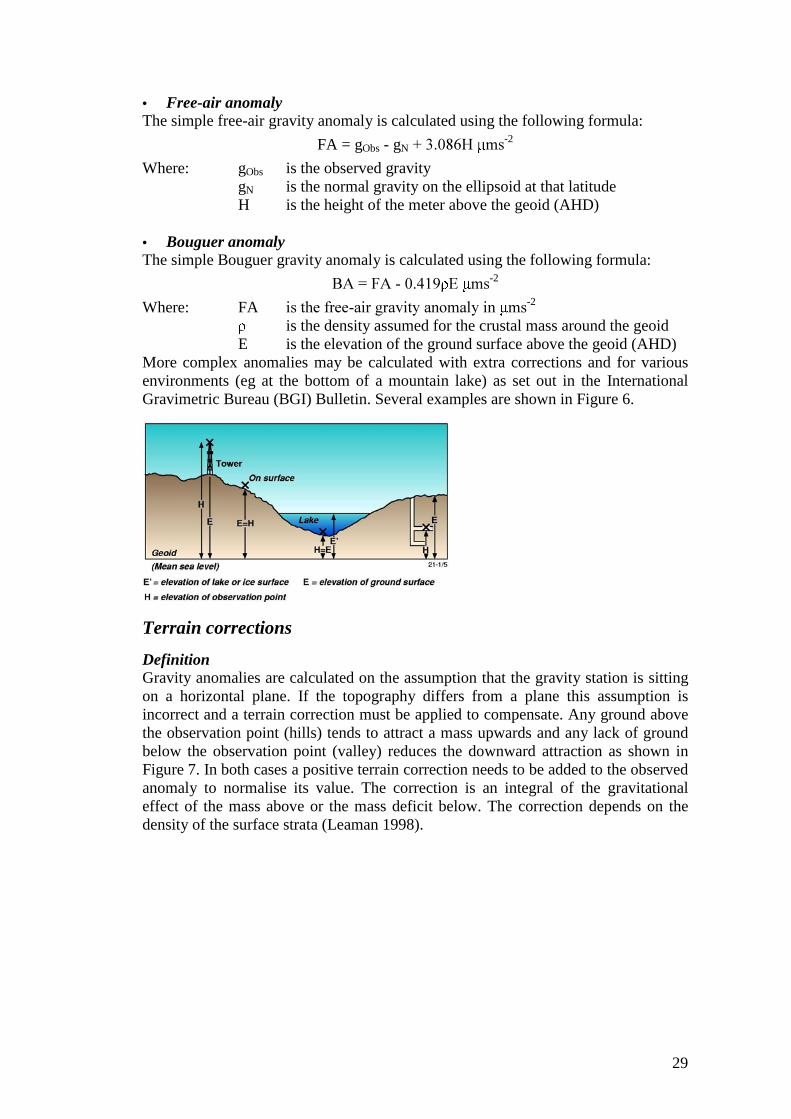
29

• Free-air anomalyThe simple free-air gravity anomaly is calculated using the following formula:

FA = gObs - gN4,��758 ��-2

Where: gObs is the observed gravitygN is the normal gravity on the ellipsoid at that latitudeH is the height of the meter above the geoid (AHD)

• Bouguer anomalyThe simple Bouguer gravity anomaly is calculated using the following formula:

/'�9'(��-�: ; ��-2

Where: FA �� (�� -2

is the density assumed for the crustal mass around the geoidE is the elevation of the ground surface above the geoid (AHD)

More complex anomalies may be calculated with extra corrections and for variousenvironments (eg at the bottom of a mountain lake) as set out in the InternationalGravimetric Bureau (BGI) Bulletin. Several examples are shown in Figure 6.

Terrain corrections

DefinitionGravity anomalies are calculated on the assumption that the gravity station is sittingon a horizontal plane. If the topography differs from a plane this assumption isincorrect and a terrain correction must be applied to compensate. Any ground abovethe observation point (hills) tends to attract a mass upwards and any lack of groundbelow the observation point (valley) reduces the downward attraction as shown inFigure 7. In both cases a positive terrain correction needs to be added to the observedanomaly to normalise its value. The correction is an integral of the gravitationaleffect of the mass above or the mass deficit below. The correction depends on thedensity of the surface strata (Leaman 1998).

30

.

Automatic corrections - what do we need?Many geophysical processing packages now include automatic terrain correctiontools. These tools require a file of the regional DTM and the near area DTM and anestimate of the ground slope at the observation point. Both DTMs must be derivedfrom the same topographic base. Australia is now covered by a 9 second (~250m)grid of elevation values. For the near area a 25m DTM is required but is not availablein most cases. Satellite radar/laser altimetry promises to provide a micro grid ofelevation in the near future.

What size effect is involved?Terrain corrections are much larger than you think, and extend for much further froma topographic feature. The maximum terrain correction for stations in the NGD is��2#� ��-2 even with sensible site selection. The effect of terrain in Australiacan extend for up to 50 kilometres.

Some quantitative examplesThe following table shows the gravity terrain effect, at various distances, of anescarpment of various heights (using 2.5D modelling). Terrain corrections are shown�� -2.

Escarpmentheight

Distance=200m 1 km 5 km 10 km 20 km 50 km

100 m 6.6 1.8 0.3 0.1 0 0

200 m 24.9 7.1 1.0 0.6 0.3 0

500 m 123.4 43.4 8.0 3.7 1.6 0.5

1000 m 344.6 157.7 32.4 14.8 6.4 1.8

Error detection and quality control

What do errors look like in lists or on maps and images?Any unexpected break in the pattern of a list or image may indicate an error. Errorscome in several forms; single station spikes, loop drift, station mis-tie, positionalshift, etc. Any significant single station anomaly is a candidate for error checking.Generally any gravity anomaly which seems to be an artefact of the data distributionshould be checked for being a systematic error.

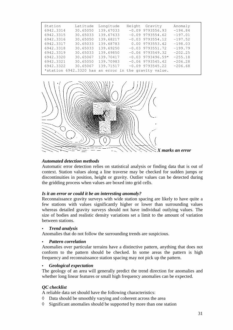
31

X marks an error

Automated detection methodsAutomatic error detection relies on statistical analysis or finding data that is out ofcontext. Station values along a line traverse may be checked for sudden jumps ordiscontinuities in position, height or gravity. Outlier values can be detected duringthe gridding process when values are boxed into grid cells.

Is it an error or could it be an interesting anomaly?Reconnaissance gravity surveys with wide station spacing are likely to have quite afew stations with values significantly higher or lower than surrounding valueswhereas detailed gravity surveys should not have individual outlying values. Thesize of bodies and realistic density variations set a limit to the amount of variationbetween stations.

• Trend analysisAnomalies that do not follow the surrounding trends are suspicious.

• Pattern correlationAnomalies over particular terrains have a distinctive pattern, anything that does notconform to the pattern should be checked. In some areas the pattern is highfrequency and reconnaissance station spacing may not pick up the pattern.

• Geological expectationThe geology of an area will generally predict the trend direction for anomalies andwhether long linear features or small high frequency anomalies can be expected.

QC checklistA reliable data set should have the following characteristics:◊ Data should be smoothly varying and coherent across the area◊ Significant anomalies should be supported by more than one station

Station Latitude Longitude Height Gravity Anomaly6942.3314 30.65050 139.67033 -0.09 9793556.93 -194.846942.3315 30.65033 139.67633 -0.09 9793554.62 -197.016942.3316 30.65050 139.68217 -0.03 9793554.12 -197.526942.3317 30.65033 139.68783 0.00 9793553.42 -198.036942.3318 30.65033 139.69250 -0.03 9793551.72 -199.796942.3319 30.65033 139.69850 -0.06 9793549.32 -202.256942.3320 30.65067 139.70417 -0.03 9793496.59* -255.186942.3321 30.65050 139.70983 -0.06 9793545.42 -206.286942.3322 30.65067 139.71517 -0.09 9793545.22 -206.68*station 6942.3320 has an error in the gravity value.

32

◊ Anomalies should not follow the boundaries of gravity surveys or traverses◊ Trends and lineaments should pass seamlessly across different gravity surveys◊ Anomaly patterns should not conflict with the mapped geology

How to rectify errors in a gravity survey

Check for gravity survey self-consistencyEach survey should be individually checked before being added to a database. Anysingle station anomalies and pieces of the survey that are inconsistent should bechecked. The problem variable should be identified as position, height or gravity bycomparing the station with its neighbours in sequence and in position.

Identifying tie points and comparing valuesThe control and tie points in the problem survey must be identified and their valueschecked against the current values for those points. In order to do this checking, thecontrol and tie points in a survey must be given the correct original number and beincluded in the data.

Statistical comparison and grid differencingTwo or more overlapping surveys may be checked by gridding the overlap area ofeach survey or group of surveys separately and comparing the statistics for the grids.A difference in average values may indicate a datum problem and a difference instandard error a scale problem. The grids may also be subtracted and the pattern ofthe difference inspected for systematic errors.

Is the projection of coordinates compatibleIf the incompatibility between surveys appears to be spatially based, the projectionsand positional datum should be checked. This may mean going back to the originaleasting and northing and checking the conversion to geographical.

Changing datum, stretching and tiltingIf a datum error has been found and corrected, care should be taken that any changeto the survey in question is also reflected in all dependent surveys. A new grid andimage should be generated for any area in which changes have been made to checkthat these changes were effective, were done properly and have not introduced anyconsequent problems. Where surveys need to be stretched or tilted to fit in withsurrounding data or because of a specific problem within the survey, great care needsto be taken to check that the result is satisfactory and to ensure that dependentsurveys are not put out of alignment. Usually the control and tie points will be fixednodes in the transformation and this should quarantine the changes to one survey.

33

The Australian Fundamental Gravity Network

The development of the AFGNThe Australian Fundamental Gravity Network (AFGN) defines the scale and datumfor gravity surveys in Australia and the surrounding oceans. The scale is used tochange differences in gravity meter readings to differences in gravity accelerationand the datum is used to convert those differences in acceleration to actualacceleration at each observation point (Wellman et al, 1985a).

The Australian Fundamental Gravity Network was established in the early 1950susing Cambridge pendulum apparatus (Dooley et al, 1961). Ties were made between59 sites with the observations relative to the station Melbourne A (AGSO stationnumber 5099.9901). Between 1964 and 1967, this network was expanded to a grid of200 sites consisting of primary stations and excentres on 14 east-west traverses and 3north-south traverses (McCracken, 1978). The east-west traverses were planned tojoin places of equal gravity and, for this reason, the network was referred to as theIsogal Network. As the variations in gravity along these traverses were limited to 50-100 µms-2, any calibration errors in the gravity meters were minimised. The north-south traverse along the east coast, known as the Australian Calibration Line(Wellman et al, 1974 and Wellman and McCracken, 1975), was used to define thescale of the network while the other two north-south traverse were used to detect anylarge errors in the network.In 1980 a survey was conducted (Wellman et al, 1985a) to strengthen this networkand increase its accuracy by taking precise measurements at 67 airports throughoutAustralia using seven LaCoste & Romberg gravity meters. Ties were also made tosix absolute gravity sites that were established in 1979 (Arnautov et al, 1979). Theseabsolute sites became the new datum for the network and for the Isogal84 values(Wellman, 1985b). Further densification of the network has taken place in later yearsas needed, such as the re-establishment of the Victorian part of the network in 1995(Murray and Wynne, 1995).

The Australian Fundamental Gravity Network currently consists of about 900stations at or near over 250 localities throughout Australia. Figure 1 shows thedistribution of these stations.

Site selectionFundamental Gravity Network Stations are preferably placed in a vibration free sitethat is sheltered from the weather and has an existing concrete base on which agravity meter can be placed. The actual reading position is marked with either a 6cmbrass disc glued to the concrete or, in more recent years, a 2.5cm blue aluminiumplug embedded in the concrete flush with the surface. Both markers are stamped withthe AGSO station number for identification.Generally, at least two stations are established at each location. The primary stationis located at the most suitable easily accessible site and at least one secondarystation, or excentre, is located at another site as a backup in case the primary stationis destroyed. Historically, most of these stations have been sited at airports becauseaircraft were used as transport when the stations were established. Redevelopment ofairport buildings over the years has resulted in many stations being destroyed.

DocumentationStation descriptions are available for all Fundamental Gravity Network Stations.These consist of one or more diagrams showing the location of the station andgenerally two photographs, one distant and one close-up. Information such as the

34

gravity value and, if available, latitude, longitude and elevation are included on thestation description. These descriptions, an example of which is shown in Figure 2,are available on request from AGSO and will soon be available on the web.

Calibration RangesA calibration range consists of two gravity stations that can be used to calibraterelative gravity meters. The Australian calibration ranges were initially establishedduring 1960 and 1961 primarily for the calibration of quartz type gravity meters(Barlow, 1967). Sites were chosen in Melbourne, Adelaide, Perth, Brisbane, Sydney,Hobart, Alice Springs and Townsville. Since then ranges have been established inCanberra, Darwin and Port Moresby. Some of the original sites have been destroyedand new sites have been established to replace them.

Most calibration ranges have a gravity interval of about 500 µms-2 because thisapproached the largest useable range for some quartz type meters. Barlow (1967)lists the following criteria that were used when selecting suitable sites for calibrationranges:1. The range should be within reasonable driving time to the area it serves.2. The gravity interval should be between 500µms-2 and 600µms-2.3. Driving time between stations should be as short as possible.4. The sites should be accessible at all times.5. The sites should be permanent.6. The sites should be easily located and obvious to a new observer.7. The sites should be free from vibration due to heavy traffic and other causes.8. The sites should preferably be sheltered from the wind and rain.

In order to obtain the required gravity interval within a short driving distance, mostranges have been located on hills, using the elevation difference to provide thedifference in gravity.

LaCoste and Romberg gravity meters are provided with a table of calibration factorscovering the full range of the instrument so it is therefore not necessary to calibratethem over the reading range that they will be operating in for a particular survey.However calibration ranges are useful to check the operation and repeatability ofthese instruments before and after a survey. Accurate calibration of these instrumentsrelative to the Australian Fundamental Gravity Network can be obtained by using anorth-south line such as the Australian Calibration Line (Wellman et al, 1985b).

International tiesThe AFGN has been tied to the world network by numerous international ties withrelative meters and by absolute measurements. A summary of international gravitymeasurements is given in Murray (1997). In the last four years a number of Japanese,French and Australian absolute measurements have been made at Mount Stromlonear Canberra.

GeodesyGeodesists use the gravity field to determine the shape of the Geoid throughout theAustralian region. The deflection of the vertical is calculated at each gravity stationto give an indication of the slope of the geoid around that point. Accurate gravitymeasurements at primary geodetic points will help to anchor these calculations. It issuggested that the primary geodetic points be included in the AFGN

35

Future Directions

Absolute MeasurementsA systematic network of absolute gravity measurements will be made throughoutAustralia at selected AFGN stations. These measurements will be used as thereference standard for readjusting the AFGN network to an absolute datum. Futureabsolute measurements are planned on geodetic points and state survey controlmarks.

GradiometryGradiometry is a new geophysical tool that provides a different view of crustaldensity variations. If measured as a full tensor, it contains more information than thevertical component of gravity, but in a qualitative rather than quantitative form. Onecomponent of the gradient tensor is the derivative of the observed gravity profile butthe gradients have no absolute gravity information so need good ground coverage toprovide the reference level.

Multi-disciplinary workLogistics are the principal costs in doing geophysical surveys. It is sensible tocombine several disciplines into one platform. This has been done for marine surveyswith seismic, gravity, magnetic and depth measurements being made simultaneously.Airborne surveys have combined magnetic, radiometric and elevation measurements.In future it should be possible to add EM and gravity gradiometry to airbornesurveys. Land surveys have combined gravity with geochemical sampling andgravity work has been done using the infrastructure from seismic surveys.

36

ReferencesArnautov, G.P., Boulanger, Yu.D., Karner, G.D., and Shcheglov, S.N., 1979 –

Absolute determination of gravity in Australia and Papua New Guinea during1979. BMR Journal of Australian Geology and Geophysics, 4, 383-393.

Barlow, B.C., 1967 – Gravity meter calibration ranges in Australia. Bureau ofMineral Resources, Australia, Report 122.

Bureau Gravimetrique International. 2000. Bulletin d'Information. 85, 14-16.

Dooley, J.C., McCarthy, E., Keating, W.D., Maddern, C.A., and Williams, L.W., 1961– Pendulum Measurements of Gravity in Australia 1950-51. Bureau of MineralResources, Australia, Bulletin 46.

Hoffman-Wellenhof, B., Lichtenegger, H., and Collins, J., 1994 – GPS Theory andPractice. Springer-Verlag Wien, 3rd Ed.

Leaman, D. E., 1984, Notes on microbarometer elevation determinations (short note):Expl. Geophys., Austr. Soc. Expl. Geophys., 15, 53-59.

Leaman, D.E., 1998. The gravity terrain correction – practical considerations. Expl.Geophys, 29, 467-471

Leick, A., 1995 – GPS Satellite Surveying. John Wiley and Sons, 2nd Ed.

Longman, I.M., 1959. Formulas for computing the tidal acceleration of the moon andthe sun. J. Geophys. Res. 64, 2351-2355.

McCracken, H.M., 1978 – Australian Gravity Network Adjustment, 1975. Bureau ofMineral Resources, Australia, Report 207; BMR Microform MF68.

Murray, A., and Wynne, P., 1995 – Fundamental gravity network in Victoria 1995 re-establishment survey. AGSO Record 1995/70.

Murray, A.S., 1997 – The Australian National Gravity Database.. AGSO Journal ofAustralian Geology and Geophysics, 17, 145-155..

Wellman, P., Boulanger, Yu,D., Barlow, B.C., Shcheglov, S.N., and Coutts, D.A.,1974 – Australian and Soviet gravity surveys along the Australian CalibrationLine. Bureau of Mineral Resources, Australia, Bulletin 161.

Wellman, P., McConnell, K., and Williams, J.W., 1985a – Australian gravity base-station network: 1980 survey. BMR Journal of Australian Geology andGeophysics, 9, 225-231.

Wellman, P., and McCracken, H.M., 1975 – Gravity measurements on Papua NewGuinea crustal movement markers, and along the Australian Calibration Line,1975. Bureau of Mineral Resources, Australia, Record 1975/126.

Wellman, P., Barlow, B.C., and Murray, A.S., 1985b – Gravity base-station networkvalues, Australia. Bureau of Mineral Resources, Australia, Report 261.

37

Appendix A: Gravity Point Located Data Interchange Standard

INTRODUCTION

At a gravity workshop organised by the Australian Geological Survey Organisation (AGSO)in Canberra on the 9th December 1999 a representative group of geoscientists responsible formanaging Australian gravity data decided that a standard should be established for theinterchange of digital gravity data, based on the ASEG-GDF2 standard. All States (exceptWestern Australia), the Northern Territory and the Commonwealth Government (AGSO andAUSLIG) were represented at the meeting. Des Fitzgerald of DFA (developer of the Intrepidgeophysical processing system) and two exploration industry representatives also attendedthe meeting. A decision was made at the conference of the Chief Government Geologists in2000 to adopt the ASEG-GDF2 standard for point located data as a minimum requirement.

AGSO is currently moving its geo-scientific databases from divers in-house andunsupported processing packages onto a corporate Oracle system. As part of this process theNational Gravity Database is being moved from an in-house database and processingsystem, which has been running for over 20 years, into an Oracle database with Intrepid asthe main data-processing system. This changeover provided an opportunity to consider theformat in which we exchange data with the States, Territories, industry and other clients.

In the move towards networked personal computers as the prime data-processing equipment,a standardised form of data exchange is becoming very important. We do not have the skilland facility to write small reformatting programs in the point-and-click environment ofWindows NT as we may have had in the command line environment of a mainframe or Unixmachine. We just want to be able to suck the data directly into a processing system or adatabase table with the minimum of effort.

The design of an Oracle point located database requires careful consideration of the requiredfields, their format and how look-up tables and acronyms are used. When dealing with adatabase of a million or more records the amount of duplication is important. Someparameters can be logically inferred from others and some can be stored in the survey meta-data table. The same philosophy and much of the structure can be carried across to the datainterchange format. Some fields in a point located gravity database or data interchange fileare critical and are common while others are more of a housekeeping concern and will bedifferent. Most data interchange involves current or new data and will tend to be a unitaryfile where all measuring units, gravity control points and positioning parameters, forexample, apply to every point value. These parameters can be specified in the meta-data fileor the definition file as defined in the ASEG-GDF2 standard (Pratt, 1994). Data may also beexchanged in projected form using northing and easting rather than latitude and longitude,and gravity anomalies rather than observed gravity values. The standard format for gravitydata interchange should be broad enough to be convenient and attractive for all types of userwhile retaining the rigour of a fully self-defining system. The software for packing andunpacking the data should be, ideally, included on the media being exchanged.

RATIONALE

What are the benefits of adopting a national standard for gravity data interchange and whychoose ASEG-GDF2? Apart from the aforementioned problem of having to keep writingreformatting code there are a number of important reasons for adopting this standard:• Discipline – having a standard that is widely publicised on the web, in literature and in

tender specifications will make creators and users of gravity data think more clearlyabout the significance of their data. The specification of mandatory fields will hopefullyovercome sloppy reporting practices in which key data fields or base-tie information are

38

omitted. Some parameters that a field operator may not consider as important, such asthe base map projection, become critical when divers data sets are assembled into anational database. Writing a standard into government tender specifications will ensurethat contracting companies become familiar with the standard and that full value can beextracted from the work performed. We can also encourage the standard being carriedover to private contracts by including it in exploration lease reporting requirements.

• Compatibility – having a commonly used standard will not only facilitate the seamlesstransfer of data between governments, industry and clients but will also encourage thesoftware developers to write the standard into the import/export tools of their processingpackages. Australia is fortunate to have several of the big geophysical or GIS softwarecompanies based in the country. The data exchange standard must also be independentof equipment and media.

• Integrity – standard specification of field definition, measurement units, base control,survey methods, equipment and accuracy will avoid mistakes and false assumptions andensure that the data are self contained and recoverable in the future. A standard thatincludes the survey meta-data will ensure that the information about timing, instruments,contractors, base control, etc. are transmitted digitally with the point data rather thanbeing filed as hard copy in one organisation’s archives.

CHOICE OF RECORDED PARAMETERS

The basic parameters or fields for an individual gravity station are those that are actuallymeasured/recorded, or derived from such, at the observation point, these are:

� Stationid – a unique station identifier usually including a survey identifier. Ifreading at an existing station the original number should be used (if known)

� Latitude or northing – may be result of GPS post-processing� Longitude or easting - may be result of GPS post-processing� Elevation of measurement point – often taken to be the ground elevation – may

be result of GPS post-processing or pressure measurements, surveying, etc.� Gravity reading – usually reduced to an (absolute) observed gravity� Elevation of ground surface or sea bottom if different from above elevation� Terrain correction – or the topographic information needed to calculate it� Station type – cell centre, repeat or tie point or normal (survey type) for example� Comments on location (eg town name), observation conditions (eg windy),

marked point (eg benchmark) or particular feature (gate, fence corner, etc.)� Gravity meter – may be put in the survey meta-data� Observer – may be put in the survey meta-data� Date and time – recorded with the field data, usually omitted for reduced data

The first five or six parameters above are mandatory for useful point data, the rest aredesirable and should be automatically included as digital data logging becomes the norm.Other information applies to the whole survey or data parcel and should be included in thesurvey meta-data or DEFN file. These parameters are:

� Survey number� Survey name� Time span of survey – start and end dates� State or country code� Position units� Estimated or actual position accuracy� Base map or projection details� Positioning method� Elevation units� Estimated or actual elevation accuracy� Elevation datum

39

� Elevation method� Gravity units� Estimated or actual gravity accuracy� Gravity reference point(s)� Gravity method� Date of processing the gravity field measurements to obtain reduced value� Terrain correction method� Contractor� Originating organisation

Many of the above parameters have traditionally been recorded in the report on the surveybut have not been stored in digital form. We should aim to capture this information digitally.Other parameters are usually not transmitted with the digital data but are stored in central ornational databases to provide a history trail of station records and access controls.

THE PROPOSED STANDARD

The proposed Point Located Gravity Data Interchange Standard allows for all the aboveparameters and gives guidelines for their definition. While complete information is desirableand will be required in future contract specifications we must accept that much of theexisting data in the National Gravity Database and other organisations’ data holdings doesnot contain all this information, or it may be too time-consuming or cost-ineffective torecover it. The standard must be flexible enough to accept as much or as little information ascan be provided.

The GDF2 standard permits three types of file for a parcel of data:• The main point located data file – one text record per observation (station). The records

may or may not have a record type label on each record.• Supporting descriptive information – the survey meta-data file (SMD). COMM type.• The GDF2 format definition file (DEFN) – may also include units and projection detail.

The gravity data interchange standard defines fields as mandatory, important and useful. Inthe descriptions that follow the standard fieldname is given in parentheses.

Definition of the mandatory fields:� Station number (stationno) – a unique gravity station or observation number applying

to the point in space where a measurement is made. This number should be usedwhen repeat measurements are made at the same point at later times. Thenumber will change if there is a change in the environment of the point leadingto a measurable change in gravity, eg: building changes, excavations or burial.The number is used as a reference to the observation in databases and digitalfiles. For the standard a 10 or 12 character format is adopted. The stationidentifier is composed of a 6-character survey label preceding a four or six digitstation number. The survey label is formed from the year and two additionalcharacters

� Latitude or Northing (latitude) – the latitude of the station in decimal degrees or thenorthing of the station in metres (projection, origin and zone details to besupplied in the survey meta-data file). Southern Hemisphere latitudes arenegative.

� Longitude or Easting (longitude) – the longitude of the station in decimal degrees orthe easting of the station in metres. Eastern Hemisphere longitudes are positive.

� Elevation (elevation) – of ground surface in metres (feet) at the position ofobservation point. The observation may be above (airborne or tower) or below(mine, tunnel, borehole) the ground surface. In marine areas this value is thewater depth.

40

� Observed gravity (obsgrav) – the gravity value tide and drift corrected and networkadjusted to the acceleration due to gravity at observation point inmicrometres.sec² or milligals. The gravity value may be specified as a free-air orBouguer anomaly but the method and density should be specified in the surveymeta-data (SMD).

� Observation elevation (obselevation) – of the gravimeter or measuring apparatus inmetres (feet) at observation point. This parameter is not mandatory ifobservation is made on the ground surface and the precise difference in heightbetween the ground surface and the measurement sensor position has not beenmeasured.

Definition of the important fields:� Survey number (surveyno) – the survey in which this (these) observations were

made. For repeat readings at a pre-existing station the survey number may differfrom the survey part of the station number. If all the data in the transmitted fileapplies to one survey this number or label should be recorded in the SMD file.

� Position units (posunits) – define the units in which the locations are recorded (egfeet, metres). This value is defined on the position DEFN records set out below.

� Coordinate frame (coordframe) – the description of the coordinate frame of referenceused for the positions (eg AMG, WGS84) recorded in the DEFN file. (see App.B)

� Reference ellipsoid (georeference) – the spheroid or geoid used for defining theframe of reference (eg Clarke 1858 Spheroid, Ausgeoid98) recorded in the SMDfile.

� Positioning method (posmethod) – defines the method in which the positions weremeasured or determined (eg GPS, photographs). Put in SMD file (see App. B).

� Elevation units (elevunits) – define the units used for the elevations (eg feet, metres).This value is defined on the elevation DEFN records set out in Appendix C.

� Elevation datum (elevdatum) – defines the datum level for the elevations (eg AHD).This parameter is specified in the SMD file but could be put on a DEFN record.

� Elevation method (elevmethod) – defines the method used to measure the elevationof the ground surface (eg GPS, barometer or survey) in SMD file (see App. B).

� Elevation type (elevtype) – describes the elevation environment of the observation(eg underground, submarine, etc.). It is mandatory if the situation is unusual andcannot be inferred from the elevation and obselevation or it is ambiguous. If allobservations are of same type this value can be put in SMD file (see App. B).

� Station type (stationtype) – classifies the station by importance based on method andquality. This important indicator of the reliability should be defined for eachstation if this is feasible. A value for the survey should be put in the SMD file

� Gravity units (obsgunits) – define the units used for the gravity values (eg milligals,micrometres). This value is defined on the obsgrav DEFN record (see App. C).

� Gravity datum (obsgdatum) – defines the datum on which the gravity values arebased. This parameter is specified in the SMD file but could be on the DEFNrecord.

� Gravity measuring method (obsgmethod) – defines the type of apparatus used for thegravity measurement (eg pendulum, Worden). Specified in SMD file (App. B).

� Gravimeter number (obsgmeterno) – specifies the number of the instrument used forthis measurement. Should be on data records where more than one meter wasused on a survey. Can be put in the SMD file if only one meter was used.

� Terrain correction (terraincorr) – is the terrain correction computed for theobservation point specified in the same units as the gravity value (obsgunits).The terrain correction may be calculated by hand using topographic informationrecorded at the point or computed from DTM heights or by statistical methods.

41

� Terrain correction density (TCdensity) – defines the density used in the terraincorrection calculations. This parameter is specified in SMD file if it is constant.

� Security classification (restriction) – is a key used to define who has access to thesedata. For most data transfers this code may be specified in the SMD file.

Definition of the useful fields:� Position error (poserror) – specifies standard deviation of the position computations

in the units used to specify the positions. For most data transfers this code maybe specified in the SMD file. This value may be estimated from the method ofdetermining positions (posmethod) but should be included when a value isknown.

� Elevation error (eleverror) – specifies standard deviation of the elevationcomputations in the units used to specify the elevation. For most data transfersthis code may be specified in the SMD file. This value may be estimated fromthe method of determining elevation (elevmethod) but should be included whenvalue is known.

� Observation date (observedate) – is the date on which the observation was made.This information is more important for base and control stations.

� Station description (stationname) – is a concise comment on location, conditions orsurvey design as exampled on page 3. It is very useful to identify tie points.

� Country or State of survey (countrycode) – indicates the country or State in whichthe measurement was made. Put in the SMD if it applies to all observationpoints.

� Gravity error (obsgerror) – specifies standard deviation of the gravity computationsin the units used to specify the gravity. For most data transfers this code may bespecified in the SMD file. This value may be estimated from the method ofdetermining gravity (obsgmethod) but should be included when a value isknown.

� Gravity calculation date (obsgcalcdate) – is of minor importance in most datatranfers but is useful in the National Database. It may be put in the SMD filewhen known.

� Observation elevation error (eleverror) – is only necessary when the computation ofthe observation and ground elevations are done independently. There may be anadditional error if the difference in heights is estimated.

� Terrain correction error (TCerror) – specifies standard deviation of the terraincorrection computations in the units used to specify the gravity. For most datatransfers this code may be specified in the SMD file. This value may beestimated from the method of determining terrain corrections (TCmethod) butshould be included when a value is known.

� Terrain Correction method (TCmethod) – defines the method used to calculate theterrain corrections. Specified in the SMD file (App. B).

� Comments – useful information or particularities of the processing history.

The standard GDF2 definition records (DEFN) for the above fields are set out in Table 1.

CONCLUSION

The Standard is reasonably straightforward and should not present much difficulty to meet,provided that it is well documented and publicised and is written into governmentexploration lease regulations and tender specifications. I recommend this Standard to theFederal, State and Territory governments, gravity survey contractors, private mineral andpetroleum exploration companies and universities as a positive step in assuring integrity andfacilitating exchange of gravity data.

42

REFERENCES

Pratt, D.A. (1994) ASEG-GDF2 – A data exchange standard for all computer users. ASEGPreview, Issue 50, 46-48.

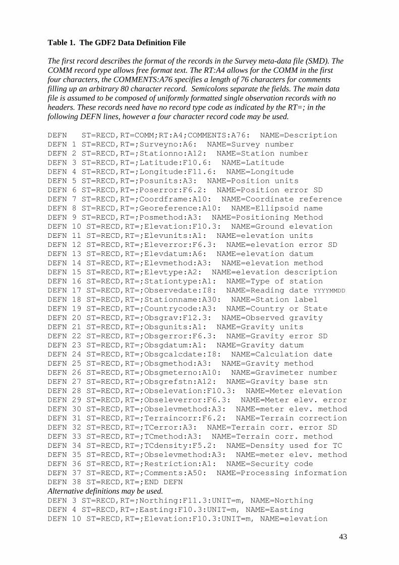
43

Table 1. The GDF2 Data Definition File

The first record describes the format of the records in the Survey meta-data file (SMD). TheCOMM record type allows free format text. The RT:A4 allows for the COMM in the firstfour characters, the COMMENTS:A76 specifies a length of 76 characters for commentsfilling up an arbitrary 80 character record. Semicolons separate the fields. The main datafile is assumed to be composed of uniformly formatted single observation records with noheaders. These records need have no record type code as indicated by the RT=; in thefollowing DEFN lines, however a four character record code may be used.

DEFN ST=RECD,RT=COMM;RT:A4;COMMENTS:A76: NAME=DescriptionDEFN 1 ST=RECD,RT=;Surveyno:A6: NAME=Survey numberDEFN 2 ST=RECD,RT=;Stationno:A12: NAME=Station numberDEFN 3 ST=RECD,RT=;Latitude:F10.6: NAME=LatitudeDEFN 4 ST=RECD,RT=;Longitude:F11.6: NAME=LongitudeDEFN 5 ST=RECD,RT=;Posunits:A3: NAME=Position unitsDEFN 6 ST=RECD,RT=;Poserror:F6.2: NAME=Position error SDDEFN 7 ST=RECD,RT=;Coordframe:A10: NAME=Coordinate referenceDEFN 8 ST=RECD,RT=;Georeference:A10: NAME=Ellipsoid nameDEFN 9 ST=RECD,RT=;Posmethod:A3: NAME=Positioning MethodDEFN 10 ST=RECD,RT=;Elevation:F10.3: NAME=Ground elevationDEFN 11 ST=RECD,RT=;Elevunits:A1: NAME=elevation unitsDEFN 12 ST=RECD,RT=;Eleverror:F6.3: NAME=elevation error SDDEFN 13 ST=RECD,RT=;Elevdatum:A6: NAME=elevation datumDEFN 14 ST=RECD,RT=;Elevmethod:A3: NAME=elevation methodDEFN 15 ST=RECD,RT=;Elevtype:A2: NAME=elevation descriptionDEFN 16 ST=RECD,RT=;Stationtype:A1: NAME=Type of stationDEFN 17 ST=RECD,RT=;Observedate:I8: NAME=Reading date YYYYMMDDDEFN 18 ST=RECD,RT=;Stationname:A30: NAME=Station labelDEFN 19 ST=RECD,RT=;Countrycode:A3: NAME=Country or StateDEFN 20 ST=RECD,RT=;Obsgrav:F12.3: NAME=Observed gravityDEFN 21 ST=RECD,RT=;Obsgunits:A1: NAME=Gravity unitsDEFN 22 ST=RECD,RT=;Obsgerror:F6.3: NAME=Gravity error SDDEFN 23 ST=RECD,RT=;Obsgdatum:A1: NAME=Gravity datumDEFN 24 ST=RECD,RT=;Obsgcalcdate:I8: NAME=Calculation dateDEFN 25 ST=RECD,RT=;Obsgmethod:A3: NAME=Gravity methodDEFN 26 ST=RECD,RT=;Obsgmeterno:A10: NAME=Gravimeter numberDEFN 27 ST=RECD,RT=;Obsgrefstn:A12: NAME=Gravity base stnDEFN 28 ST=RECD,RT=;Obselevation:F10.3: NAME=Meter elevationDEFN 29 ST=RECD,RT=;Obseleverror:F6.3: NAME=Meter elev. errorDEFN 30 ST=RECD,RT=;Obselevmethod:A3: NAME=meter elev. methodDEFN 31 ST=RECD,RT=;Terraincorr:F6.2: NAME=Terrain correctionDEFN 32 ST=RECD,RT=;TCerror:A3: NAME=Terrain corr. error SDDEFN 33 ST=RECD,RT=;TCmethod:A3: NAME=Terrain corr. methodDEFN 34 ST=RECD,RT=;TCdensity:F5.2: NAME=Density used for TCDEFN 35 ST=RECD,RT=;Obselevmethod:A3: NAME=meter elev. methodDEFN 36 ST=RECD,RT=;Restriction:A1: NAME=Security codeDEFN 37 ST=RECD,RT=;Comments:A50: NAME=Processing informationDEFN 38 ST=RECD,RT=;END DEFNAlternative definitions may be used.DEFN 3 ST=RECD,RT=;Northing:F11.3:UNIT=m, NAME=NorthingDEFN 4 ST=RECD,RT=;Easting:F10.3:UNIT=m, NAME=EastingDEFN 10 ST=RECD,RT=;Elevation:F10.3:UNIT=m, NAME=elevation

BEST PRACTICE IN GRAVITY SURVEYING - Geoscience Australia · BEST PRACTICE IN GRAVITY SURVEYING...

Documents

Transcript of BEST PRACTICE IN GRAVITY SURVEYING - Geoscience Australia · BEST PRACTICE IN GRAVITY SURVEYING...