Bernhard Steinberger

Dynamic topography

Deutsches GeoForschungsZentrum, Potsdam and

Centre for Earth Evolution and Dynamics, Univ. Oslo

What is dynamic topography?Commonly vertical displacement of the Earth's surface generated in response to flow in the Earth's mantle called “dynamic topography”

→ An effort to determine which part of topography is not due to crustal isostasy or ocean floor cooling

12

4

3

Contributions to topography (1) crustal isostasy (remove)(2) due to ocean floor cooling (remove)(3) other contributions within the lithosphere (~ isostatic – include)(4) beneath the lithosphere (“dynamic” in the proper sense – include)

Key point: Isostatic (3) and dynamic (4) topography very similar for shallow depth and large lateral scales, so don't distinguish for present day. But distinction important for time changes as (3) moves with plates (no change) and (4) doesn't (causes uplift and subsidence)

→ An effort to determine which part of topography is not due to crustal isostasy or ocean floor cooling

12

4

3

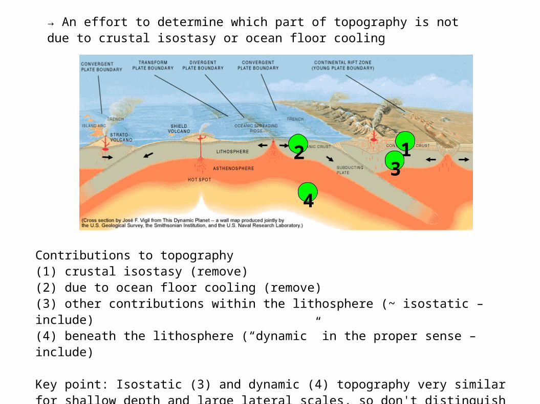
Density anomalies (3) and (4) can be inferred from seismic tomography, but lithosphere has also compositional anomalies.

Hence we are concerned with(a) which part of tomographic anomalies to include and which part not (and also, which tomography model(s) to use)(b) how to infer topography from the geoid

An important ingredient is a model of lithosphere thickness

→ An effort to determine which part of topography is not due to crustal isostasy or ocean floor cooling

12

4

3

To check the quality of our models, we compare(A) a model of “residual topography”, obtained by subtracting contributions (1) and (2) from actual topography(B) a model of topography due to contributions (3) and (4) obtained from seismic tomography (and deciding which parts to include) and subtracting contribution (2). (C) a model additionally based on the geoid

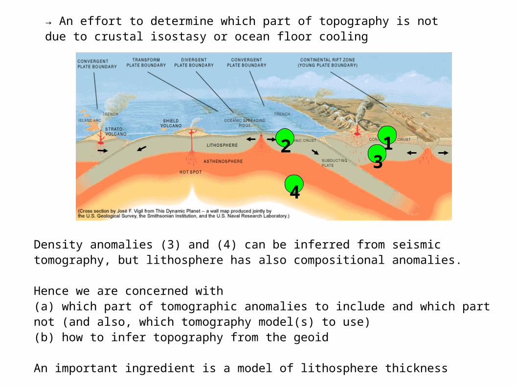
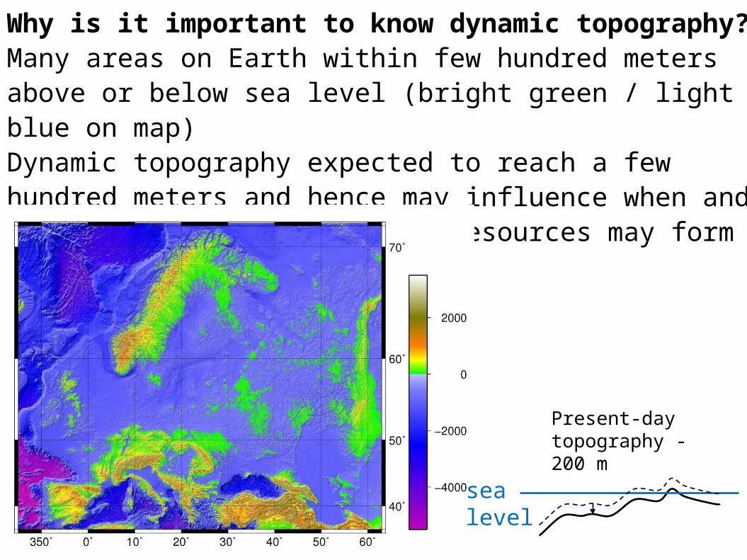
Why is it important to know dynamic topography?Many areas on Earth within few hundred meters above or below sea level (bright green / light blue on map)Dynamic topography expected to reach a few hundred meters and hence may influence when and where sediments and natural resources may form

Present-day topography

sealevel

Why is it important to know dynamic topography?Many areas on Earth within few hundred meters above or below sea level (bright green / light blue on map)Dynamic topography expected to reach a few hundred meters and hence may influence when and where sediments and natural resources may form

Present-day topography + 200 m

sealevel

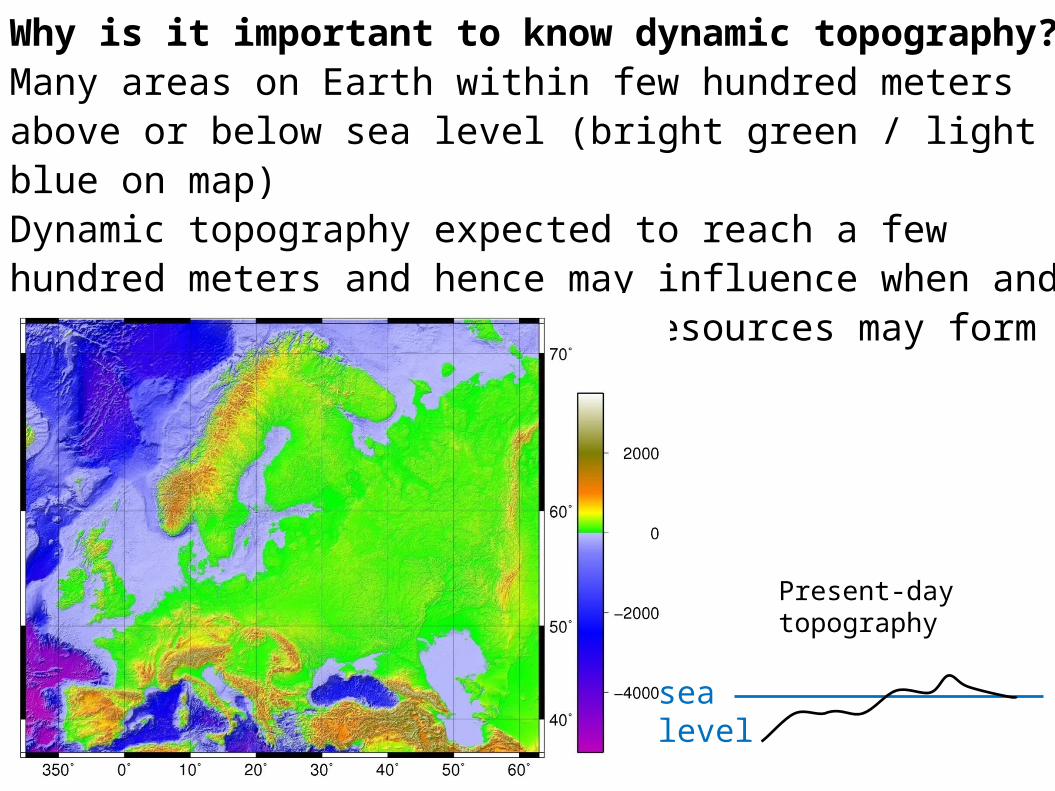
Why is it important to know dynamic topography?Many areas on Earth within few hundred meters above or below sea level (bright green / light blue on map)Dynamic topography expected to reach a few hundred meters and hence may influence when and where sediments and natural resources may form

Present-day topography - 200 m

sealevel

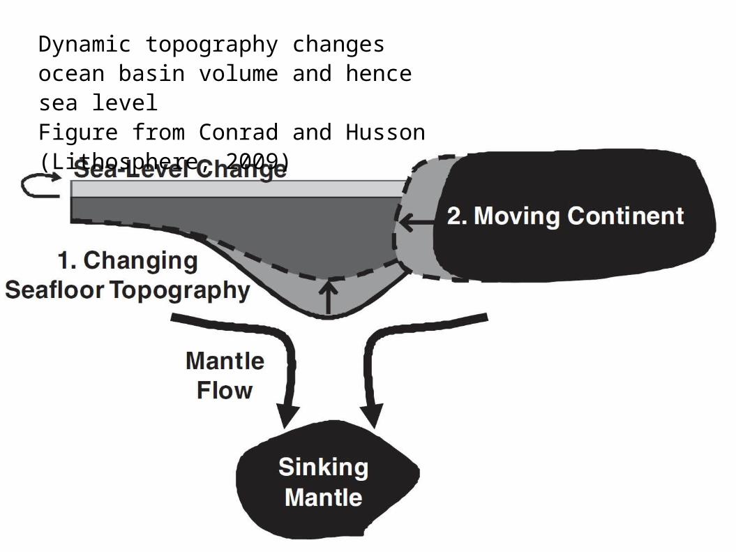
Dynamic topography changes ocean basin volume and hence sea level Figure from Conrad and Husson (Lithosphere, 2009)

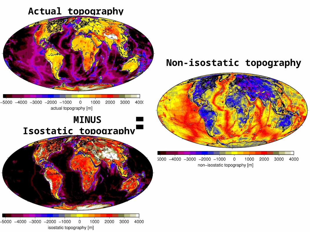
Actual topography

MINUSIsostatic topography

Airy Pratt

Inferring dynamic topography from observations

Computed based on densities and thicknesses of crustal layers in CRUST 1.0 model (Laske et al., http://igppweb.ucsd.edu/~gabi/crust1.html

Actual topography

MINUSIsostatic topography

Non-isostatic topography

=

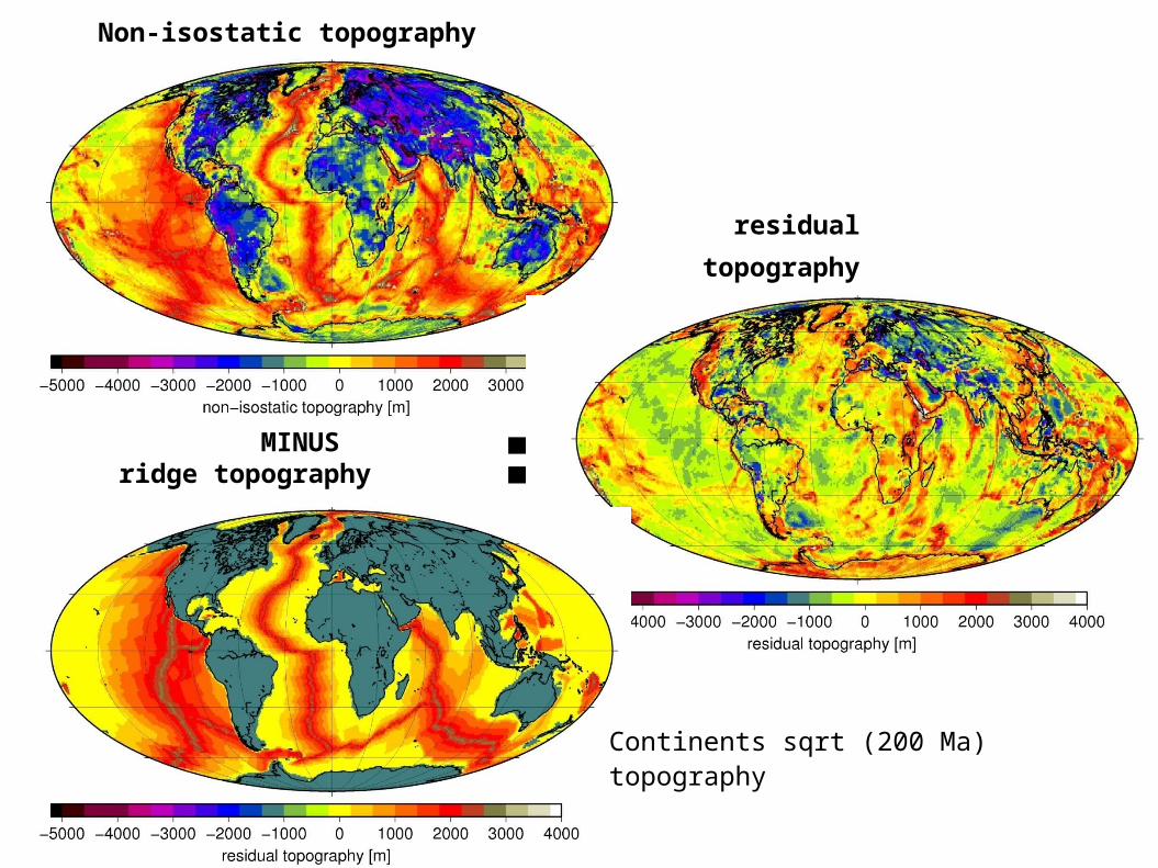
Non-isostatic topography

residual topography

MINUSridge topography =

Continents sqrt (200 Ma) topography

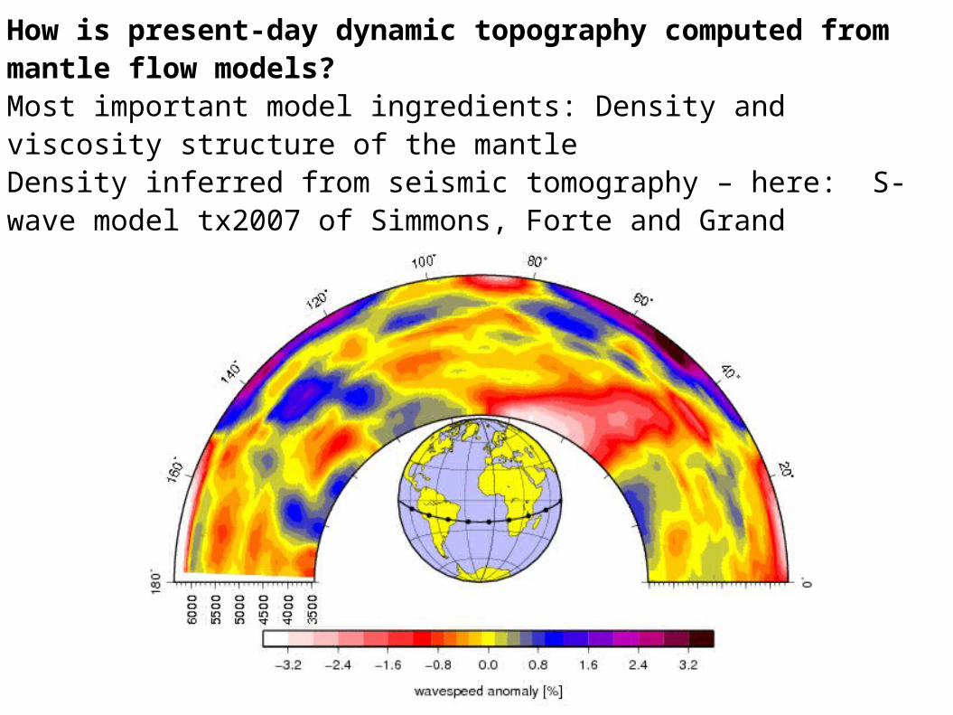
How is present-day dynamic topography computed from mantle flow models?Most important model ingredients: Density and viscosity structure of the mantleDensity inferred from seismic tomography – here: S-wave model tx2007 of Simmons, Forte and Grand

Seismic tomography

Convert to density anomalies

Blue line:Conversion factorfor thermal anomaliesinferred from mineralPhysics (Steinbergerand Calderwood, 2006)

Blue line:Conversion factorfor thermal anomaliesinferred from mineralPhysics (Steinbergerand Calderwood, 2006)

Here: attempt to “remove lithosphere” by setting density anomaly to 0.2 % wherever, above 400 km depth, inferred density anomaly is positive >0.2 % at that depth and everywhere above

Seismic tomography

Convert to density anomalies

Blue line:Conversion factorfor thermal anomaliesinferred from mineralPhysics (Steinbergerand Calderwood, 2006)

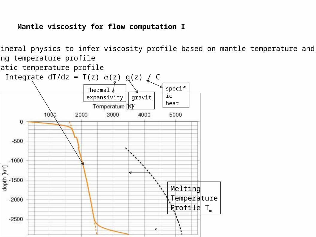
Mantle viscosity for flow computation I

Use mineral physics to infer viscosity profile based on mantle temperature and melting temperature profileAdiabatic temperature profile T(z): Integrate dT/dz = T(z) a(z) g(z) / C

Thermalexpansivity gravity

specific heat

Melting TemperatureProfile Tm

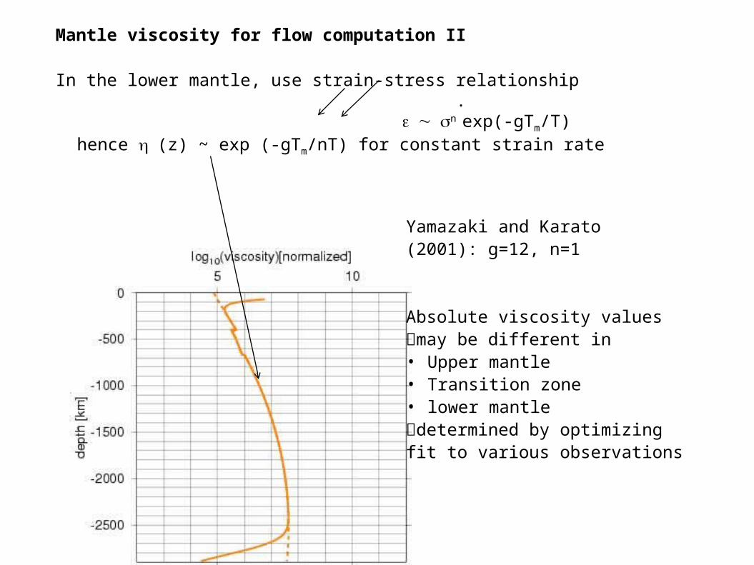
Mantle viscosity for flow computation II

In the lower mantle, use strain-stress relationship . ~ e sn exp(-gTm/T) hence h (z) ~ exp (-gTm/nT) for constant strain rate

Yamazaki and Karato(2001): g=12, n=1

Absolute viscosity valuesmay be different in• Upper mantle• Transition zone• lower mantledetermined by optimizingfit to various observations

Mantle flow computation• Density model based on tomography (here: Simmons,

Forte, Grand, 2006)

• velocity-density scaling based on mineral physics

• radial viscosity structure based on mineral physics and optimizing fit to geoid etc. (Steinberger and Calderwood, 2006)

• Spectral method (Hager and O'Connell, 1979, 1981)

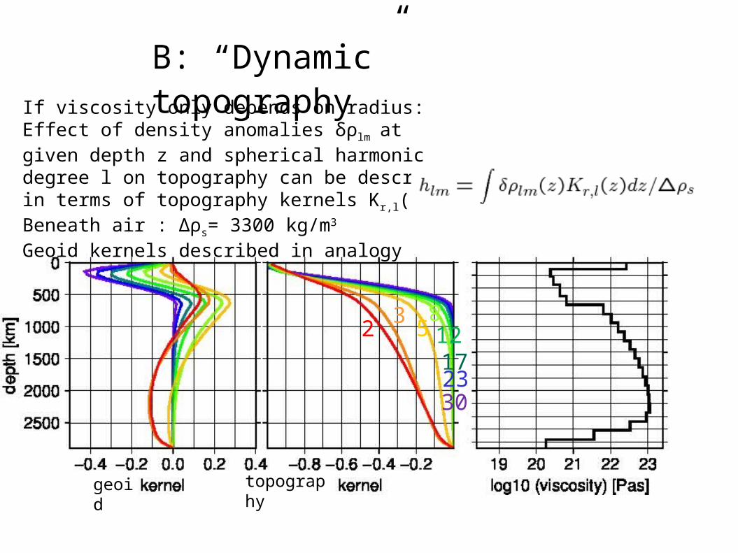
If viscosity only depends on radius:Effect of density anomalies δρlmat given depth z and spherical harmonic degree l on topography can be described in terms of topography kernels Kr,l(z):Beneath air : Δρs= 3300 kg/m3

Geoid kernels described in analogy

23

5

8

1217

3023

geoid topography

B: “Dynamic” topography

B: “Dynamic” topography: Why this is new (and exciting) (I) Recent tomography models have reached a new quality:Higher correlation with geoid in a degree and depth range where this is expected, based on kernels and amplitudes

B: “Dynamic” topography: Why this is new (and exciting) (ii) Based on new tomography models, develop a model of lithosphere thickness (and compare with other models)

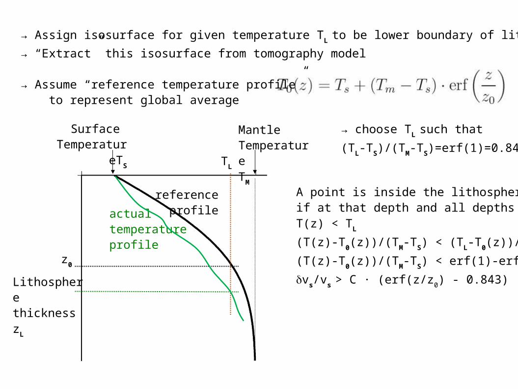
→ Assign isosurface for given temperature TL to be lower boundary of lithosphere

→ “Extract” this isosurface from tomography model

→ Assume “reference temperature profile” to represent global average

Surface TemperatureT

S

Mantle TemperatureT

MT

L

z0

referenceprofile

→ choose TL such that

(TL-T

S)/(T

M-T

S)=erf(1)=0.843

Lithosphere thickness z

L

actualtemperatureprofile

A point is inside the lithosphere,if at that depth and all depths aboveT(z) < T

L

(T(z)-T0(z))/(T

M-T

S) < (T

L-T

0(z))/(T

M-T

S)

(T(z)-T0(z))/(T

M-T

S) < erf(1)-erf(z/z

0)

vs/v

s > C · (erf(z/z0) - 0.843)

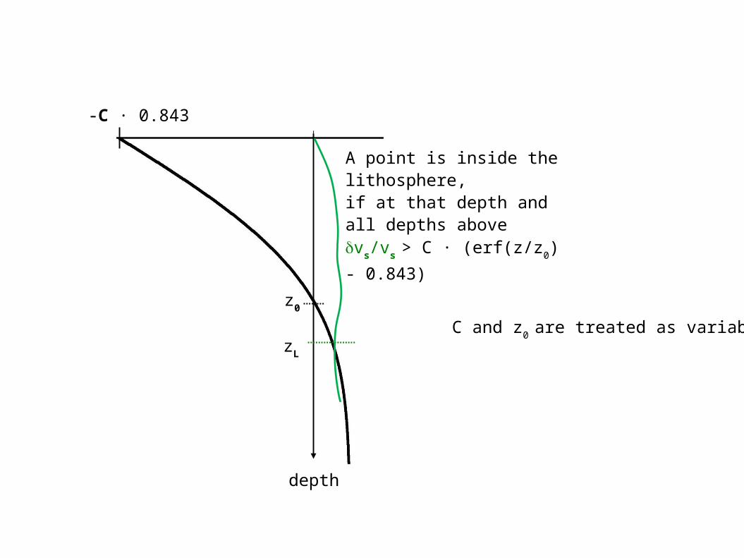
A point is inside the lithosphere,if at that depth and all depths abovev

s/v

s > C · (erf(z/z0) -

0.843)

z0

-C · 0.843

depth

C and z0 are treated as variables z

L

age_3.6 ocean floor age grid (Müller, Sdrolias, Gaina and Roest, G3, 2008)

t = ocean floor age = thermal diffusivity

For

→ determine for each point lithosphere thickness based on tomography model according to above-described procedure→ find parameters C and z

0 such that optimum fit with

is achieved for average thickness at given sea floor age.

SL2013SV:Schaeffer and Lebedev (2013)C = 9 %, z

0 = 60 km

theoretical: C = 11 %

Rychert et al. (2010) scattered wave imaging Artemieva (2006) thermal model

Priestley and McKenzie (2013) based on surface wave tomography

This model based on SL2013 tomography

Elastic lithosphere thicknessAudet and Burgmann (2011) Based on smean tomography

lRF = Rychert

1/q= 1/(heat flow) from Davies

lT = Artemieva

hC = crustal

thickness crust1

lST = simple

thickness from isovalue 

lSB = this work

seismological thickness

Te = elastic

thickness from Audet and Burgmann (2011)

→ Lithosphere = 0.2 %→ optimizedviscosity Structure→ l

max = 31

Correlation 0.77Ratio 1.08

Residual topography (before spherical harmonic expansion) divided by 1.45 in oceans to account for water coverage

Sea floor age contribution not subtracted

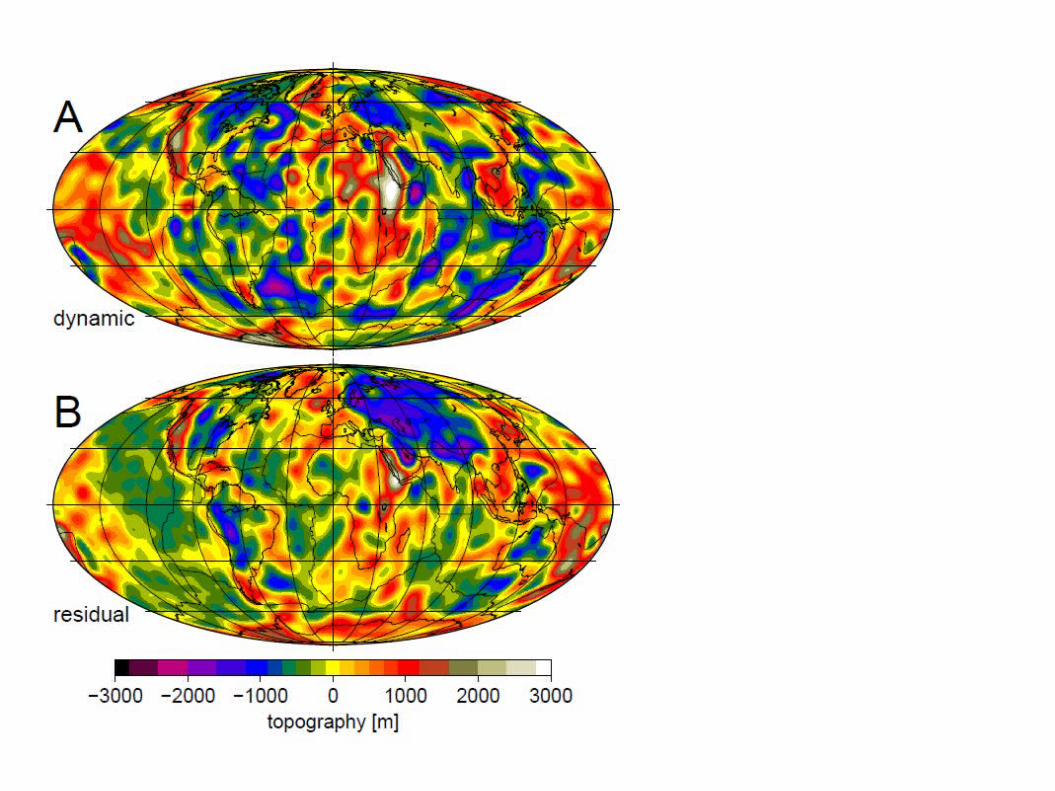
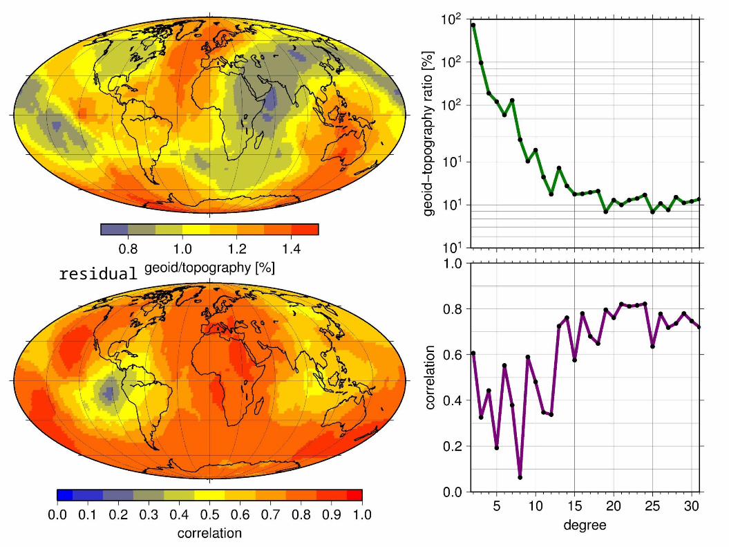
residual

Correlation and ratio of residual and “dynamic” and topography based on varioustomography models.Pink line = geoid-derived for l>~15

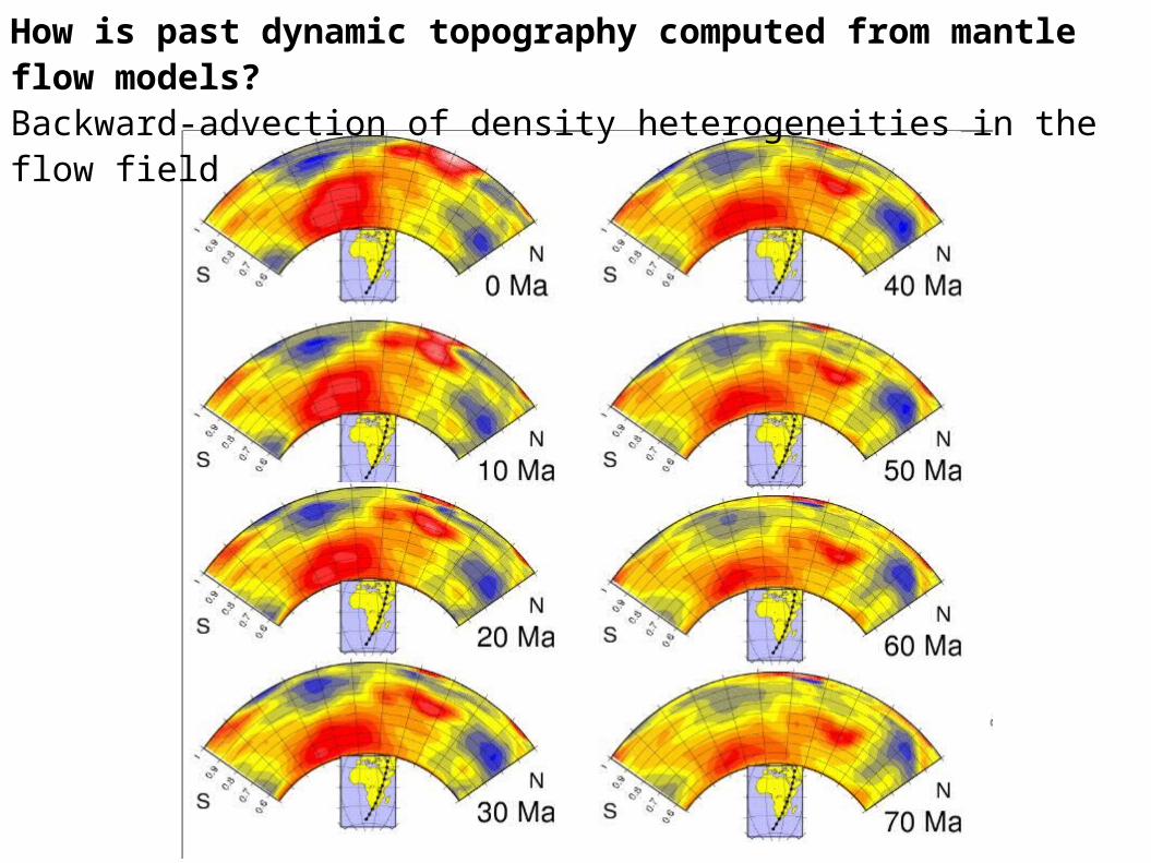
How is past dynamic topography computed from mantle flow models?Backward-advection of density heterogeneities in the flow field

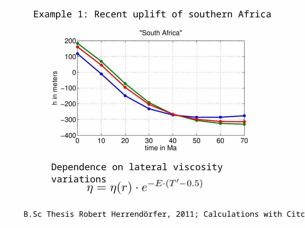
Dependence on lateral viscosity variations

B.Sc Thesis Robert Herrendörfer, 2011; Calculations with CitcomS

Example 1: Recent uplift of southern Africa

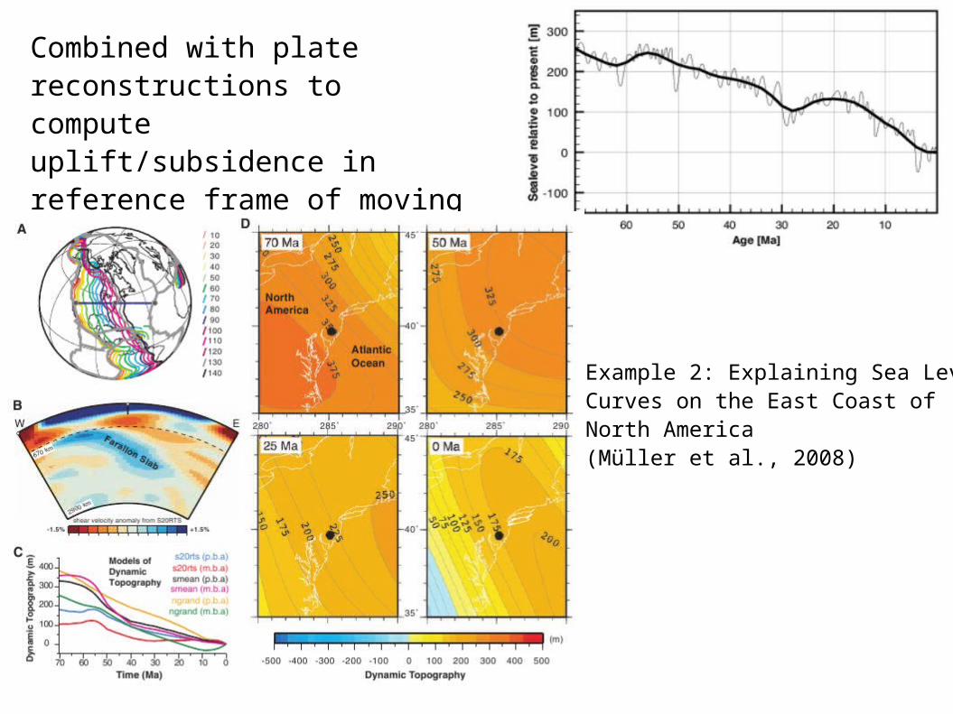
Combined with plate reconstructions to compute uplift/subsidence in reference frame of moving plate

Example 2: Explaining Sea LevelCurves on the East Coast ofNorth America (Müller et al., 2008)

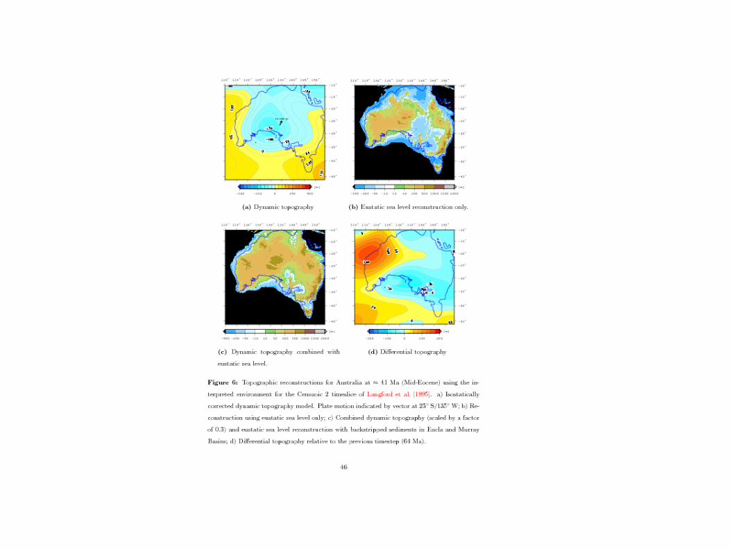
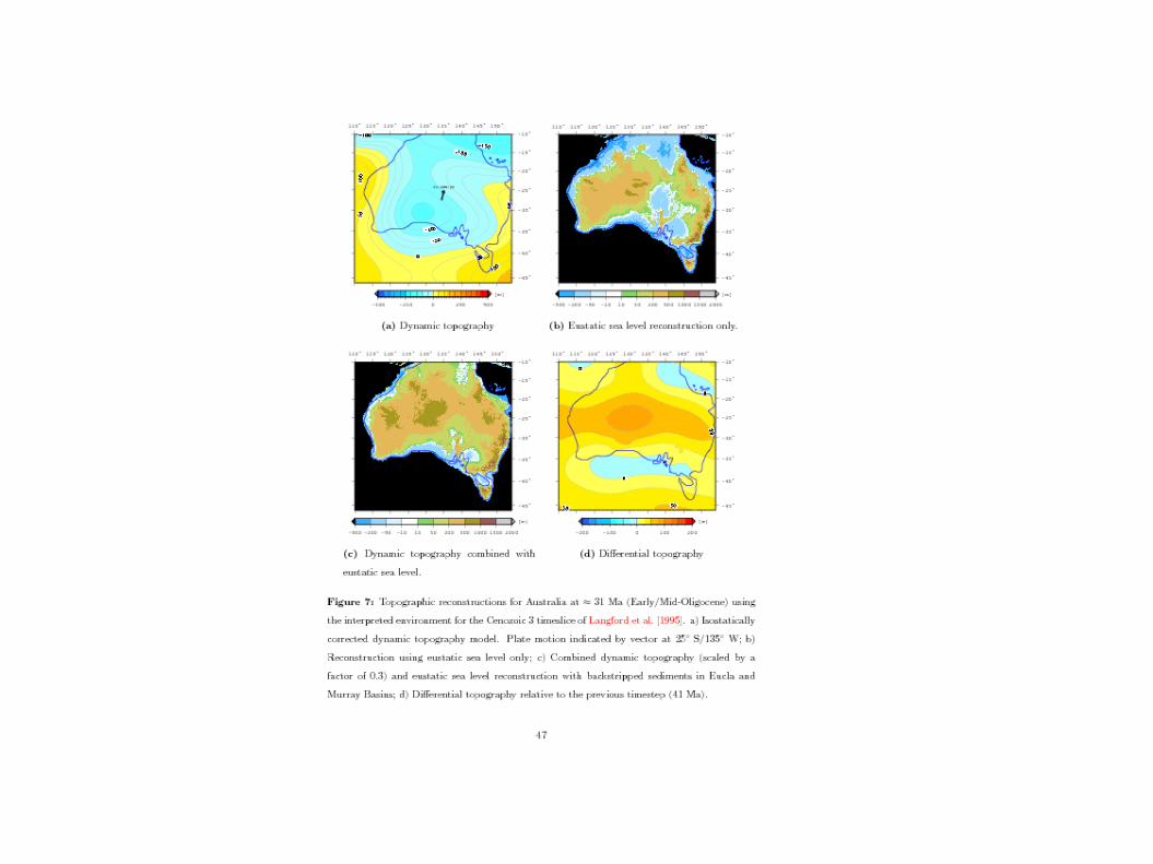
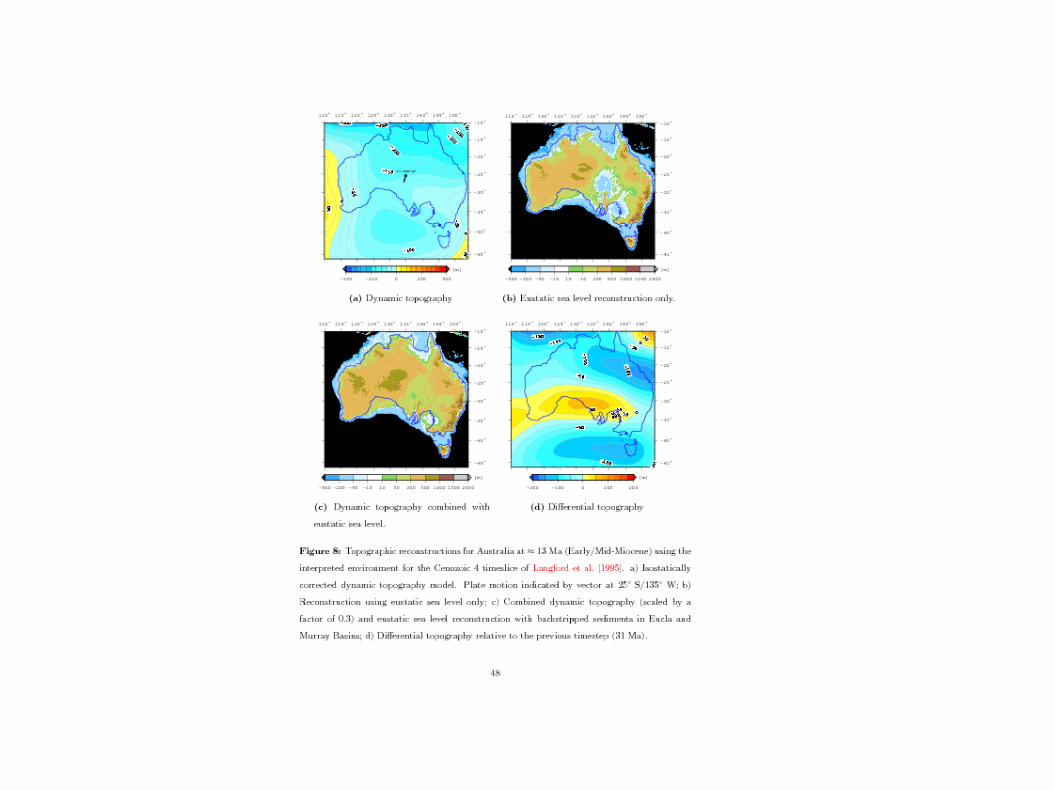
Example 3: Explaining marine inundations in Australia (Heine et al., 2009)

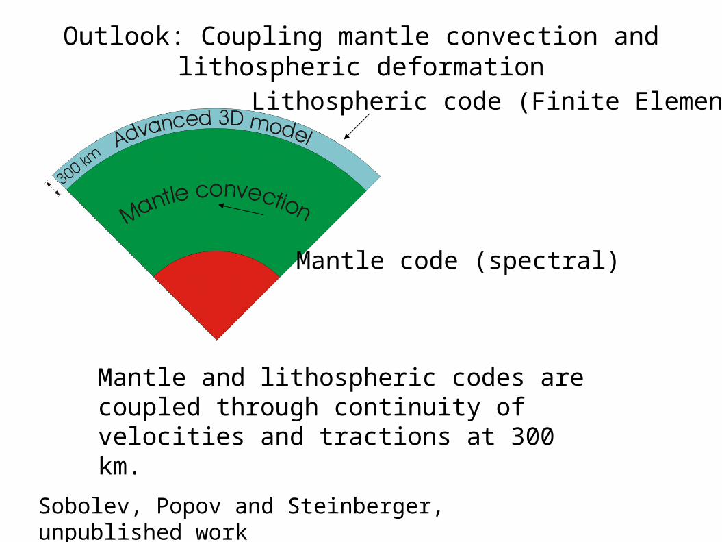
Mantle and lithospheric codes are coupled through continuity of velocities and tractions at 300 km.

Lithospheric code (Finite Elements)

Mantle code (spectral)

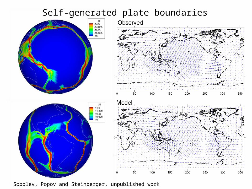
Outlook: Coupling mantle convection and lithospheric deformation

Sobolev, Popov and Steinberger, unpublished work

Sobolev, Popov and Steinberger, unpublished work

Self-generated plate boundaries

Conclusions

• Recent tomography models (in particular SL2013SV) have high correlation with geoid at intermediate degrees (l~4-50) and shallow depth, indicating substantial improvement

• Based on tomography models, we developed models of lithosphere thickness• We investigated correlation between lithosphere thickness models based on

various approaches• Rather high correlation between tomography-based and elastic thickness

estimate, but elastic lithosphere ~3 times thinner• Improved correlation between residual and „dynamic“ topography ~0.6