
Bentley RM Bridge Seismic Design and Analysis Alexander Mabrich, PE, Msc.
45
Bentley RM Bridge Seismic Design and Analysis Alexander Mabrich, PE, Msc
-
Upload
grant-flowers -
Category
Documents
-
view
225 -
download
10
Transcript of Bentley RM Bridge Seismic Design and Analysis Alexander Mabrich, PE, Msc.

Bentley RM Bridge Seismic Design and Analysis
Alexander Mabrich, PE, Msc

AGENDA
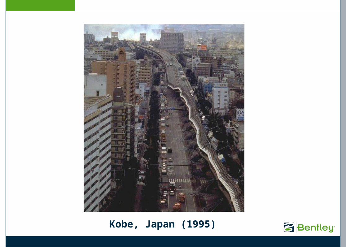
Kobe, Japan (1995)

AGENDA
Loma Prieta, California (1989)
RM Bridge Seismic Design and Analysis
• Critical infrastructures require:
– Sophisticated design methods
– Withstand collapse in earthquake occurrences

RM Bridge Seismic Design and Analysis
• AASTHO, Simple Seismic Load
• Basic concepts for Dynamic Analysis:
- Eigenvalues
- Eigenshapes
• Two non-linear dynamic options:
- Response Spectrum
- Time-History

AASHTO Bridge Design Specifications
• 7% probability of exceedence in 75years
• Seismic Design Categories
– Soil
– Site / location
– Importance
• Earthquake Resistant System
• Demand/Capacity
8 | WWW.BENTLEY.COM

• Site Location
AASHTO Bridge Design Specifications

• Type of Seismic Analysis Required
AASHTO Bridge Design Specifications
Static Seismic Load
11 | WWW.BENTLEY.COM
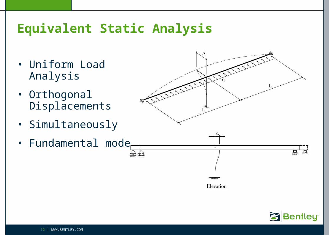
Equivalent Static Analysis
• Uniform Load Analysis
• Orthogonal Displacements
• Simultaneously
• Fundamental mode
12 | WWW.BENTLEY.COM
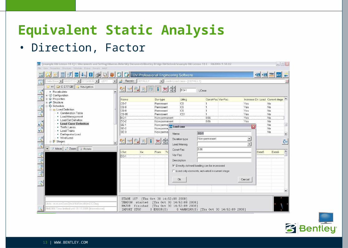
Equivalent Static Analysis• Direction, Factor
13 | WWW.BENTLEY.COM
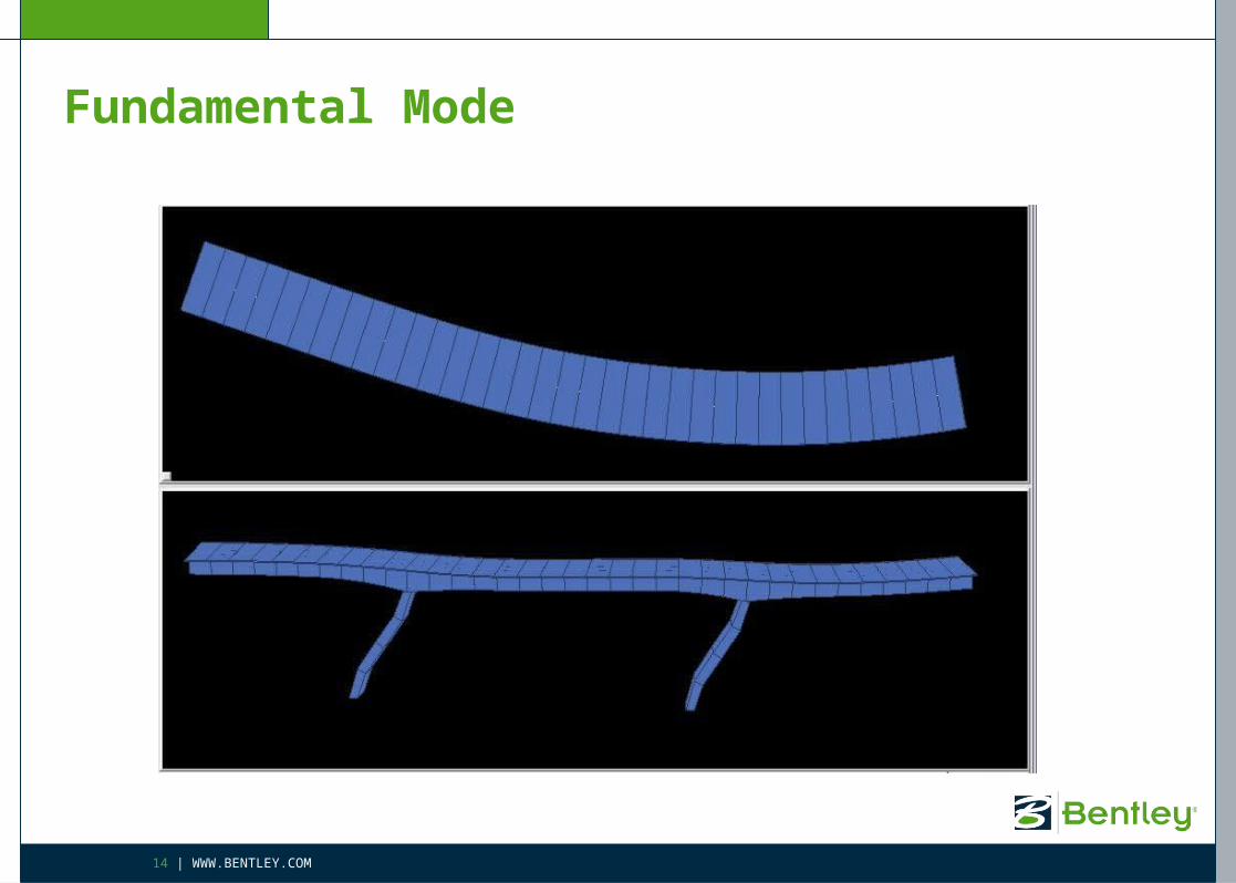
Fundamental Mode
14 | WWW.BENTLEY.COM
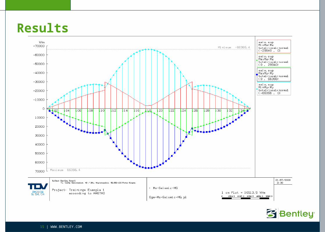
Results
15 | WWW.BENTLEY.COM
16 | WWW.BENTLEY.COM
Basic Concepts used inDynamic Analysis
Basic Concepts
• Vibration of Systems with one or more DOF
• Eigen values and Eigen modes
• Forced Vibration– Harmonic and Stochastic Simulation
• Linear and Non-linear behavior of the structure
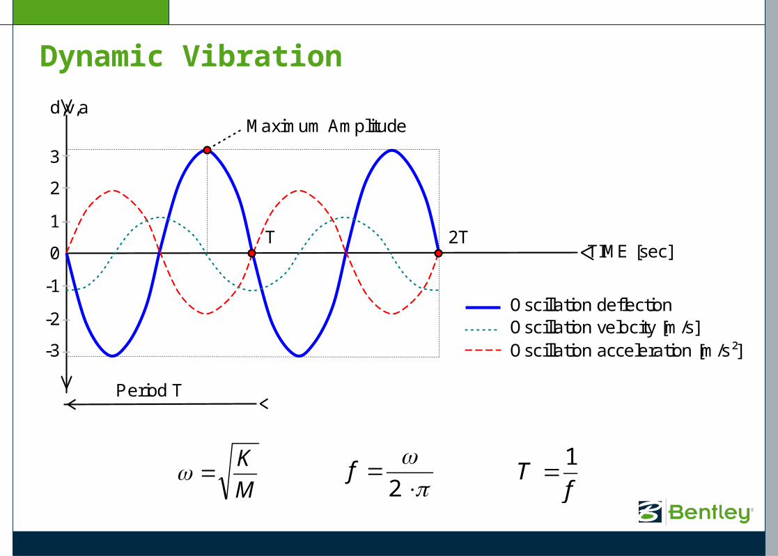
Dynamic Vibration
T 2T 1
2
3
-1
-2
-3
0 TIME [sec]
Oscillation deflection [m] Oscillation velocity [m/s] Oscillation acceleration [m/s²]
Maximum Amplitude
Period T
d,v,a
M
K
2
ff
T1
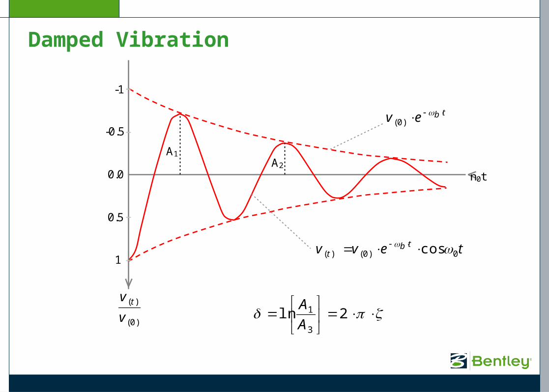
Damped Vibration
)0(
)(
v
v t
n0t
tevv tbt 0)0()( cos
tbev )0(
-1
1
0.5
-0.5
0.0
A1 A2
2ln
3
1
A
A
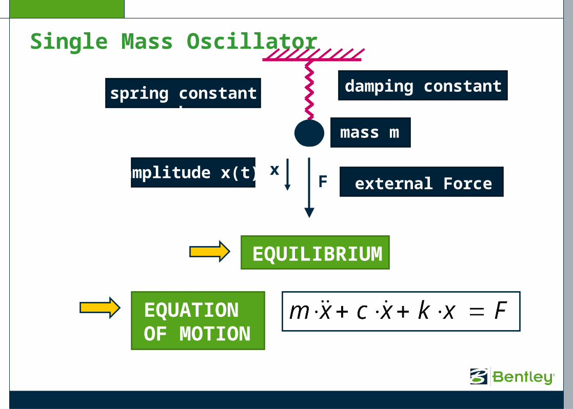
Single Mass Oscillator
spring constant k damping constant c
xF
mass m
external Force F(t)amplitude x(t)
EQUILIBRIUM
EQUATION OF MOTION

Damping Ratio
c0: 20
2
22
m
c
m
cs
t
u
=100%
t
u
t
u
=200%
t
u
=0%
=10%
Critic damping
Not damped
Below critic damping Above critic damping

0 kuucum
tutu
tu 00 sinsin)(
Solution:
Free Vibration
M
K
0c …no damping…and dividing by m…
0 um
ku But..
02 uu
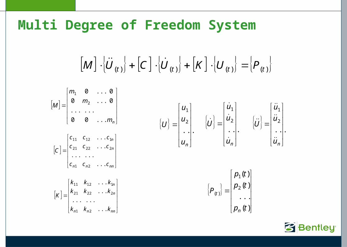
Multi Degree of Freedom System
)()()()( tttt PUKUCUM
nm
m
m
M
...00
......
0...0
0...0
2
1
nnnn
n
n
ccc
ccc
ccc
C
...
......
...
...
21
22221
11211
nnnn
n
n
kkk
kkk
kkk
K
...
......
...
...
21
22221
11211
nu
u
u
U...
2
1
nu
u
u
U
...
2
1
nu
u
u
U
...
2
1
)(
...
)(
)(
2
1
)(
tp
tp
tp
P
n
t

Numerical Methods for Dynamic Analysis
• Calculation of Eigen frequency
• Modal Analysis
• Direct Time integration, linear and non-linear
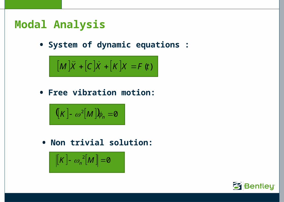
• System of dynamic equations :
)(tFXKXCXM
• Free vibration motion:
02 nMK
• Non trivial solution:
02 MK n
Modal Analysis
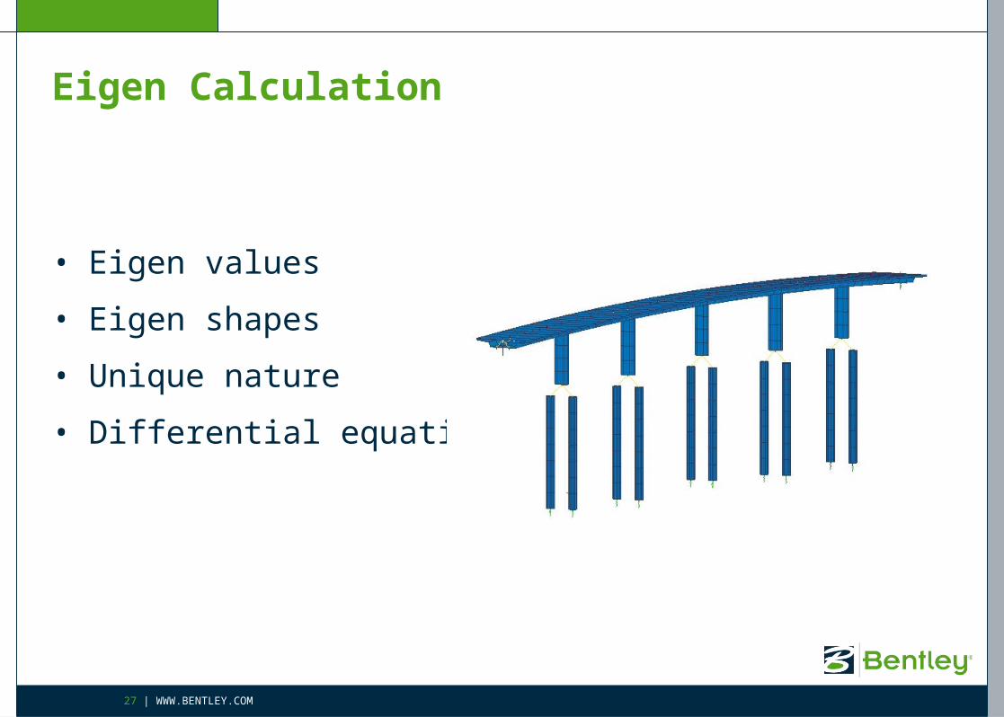
Eigen Calculation
• Eigen values
• Eigen shapes
• Unique nature
• Differential equations
27 | WWW.BENTLEY.COM
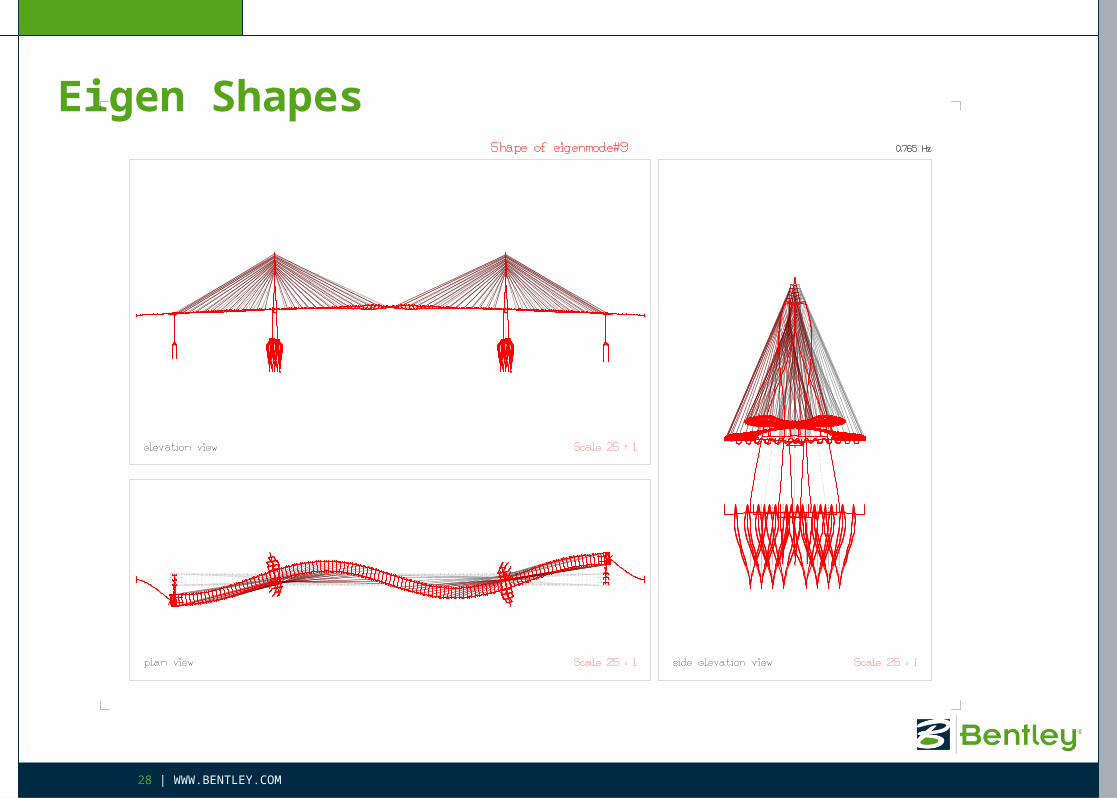
Eigen Shapes
28 | WWW.BENTLEY.COM
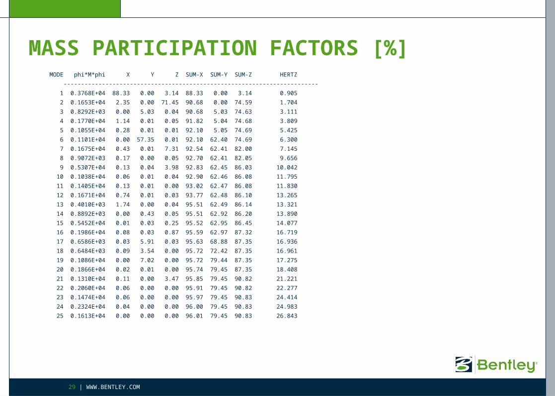
MASS PARTICIPATION FACTORS [%] MODE phi*M*phi X Y Z SUM-X SUM-Y SUM-Z HERTZ
-------------------------------------------------------------------------
1 0.3768E+04 88.33 0.00 3.14 88.33 0.00 3.14 0.905
2 0.1653E+04 2.35 0.00 71.45 90.68 0.00 74.59 1.704
3 0.8292E+03 0.00 5.03 0.04 90.68 5.03 74.63 3.111
4 0.1770E+04 1.14 0.01 0.05 91.82 5.04 74.68 3.809
5 0.1055E+04 0.28 0.01 0.01 92.10 5.05 74.69 5.425
6 0.1101E+04 0.00 57.35 0.01 92.10 62.40 74.69 6.300
7 0.1675E+04 0.43 0.01 7.31 92.54 62.41 82.00 7.145
8 0.9072E+03 0.17 0.00 0.05 92.70 62.41 82.05 9.656
9 0.5307E+04 0.13 0.04 3.98 92.83 62.45 86.03 10.042
10 0.1038E+04 0.06 0.01 0.04 92.90 62.46 86.08 11.795
11 0.1405E+04 0.13 0.01 0.00 93.02 62.47 86.08 11.830
12 0.1671E+04 0.74 0.01 0.03 93.77 62.48 86.10 13.265
13 0.4010E+03 1.74 0.00 0.04 95.51 62.49 86.14 13.321
14 0.8892E+03 0.00 0.43 0.05 95.51 62.92 86.20 13.890
15 0.5452E+04 0.01 0.03 0.25 95.52 62.95 86.45 14.077
16 0.1986E+04 0.08 0.03 0.87 95.59 62.97 87.32 16.719
17 0.6586E+03 0.03 5.91 0.03 95.63 68.88 87.35 16.936
18 0.6484E+03 0.09 3.54 0.00 95.72 72.42 87.35 16.961
19 0.1086E+04 0.00 7.02 0.00 95.72 79.44 87.35 17.275
20 0.1866E+04 0.02 0.01 0.00 95.74 79.45 87.35 18.408
21 0.1310E+04 0.11 0.00 3.47 95.85 79.45 90.82 21.221
22 0.2060E+04 0.06 0.00 0.00 95.91 79.45 90.82 22.277
23 0.1474E+04 0.06 0.00 0.00 95.97 79.45 90.83 24.414
24 0.2324E+04 0.04 0.00 0.00 96.00 79.45 90.83 24.983
25 0.1613E+04 0.00 0.00 0.00 96.01 79.45 90.83 26.843
29 | WWW.BENTLEY.COM
Response SpectrumModal Decomposition
30 | WWW.BENTLEY.COM
Response Spectrum
• Combination of natural modes
• One mass oscillator
• Oscillating loads
• Intensity factor
• Single contribution
• Synchronization by Stochastic Calculation Rules: ABS,SRSS,CQC, etc

Spectral Response Acceleration
32 | WWW.BENTLEY.COM
AASHTO Definition
Solution in Frequency Domain
• Solution by combining the contributions of the eigenvectors
• Superposition of eigenvectors– Loading has lost information about correlation during
conversion– Solution has no information on phase differences
between the contributions of different eigenvectorsUse Stochastic methodology
• Use Stochastic methodology
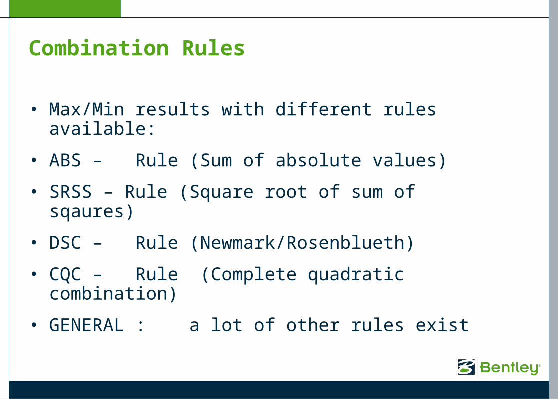
Combination Rules
• Max/Min results with different rules available:
• ABS – Rule (Sum of absolute values)
• SRSS – Rule (Square root of sum of sqaures)
• DSC – Rule (Newmark/Rosenblueth)
• CQC – Rule (Complete quadratic combination)
• GENERAL : a lot of other rules exist

Earthquake Load

Response Spectrum in RM Bridge

Time-HistoryTime Integration
41 | WWW.BENTLEY.COM
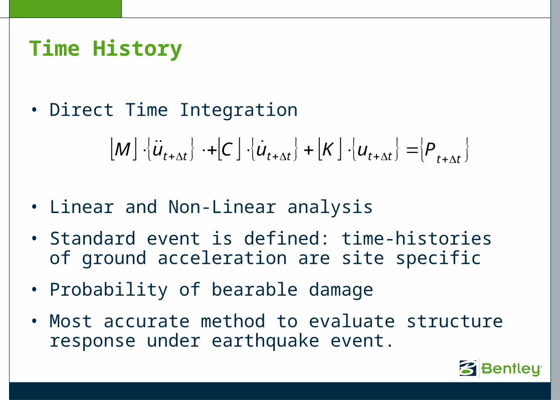
Time History
• Direct Time Integration
• Linear and Non-Linear analysis
• Standard event is defined: time-histories of ground acceleration are site specific
• Probability of bearable damage
• Most accurate method to evaluate structure response under earthquake event.
tttttttt PuKuCuM
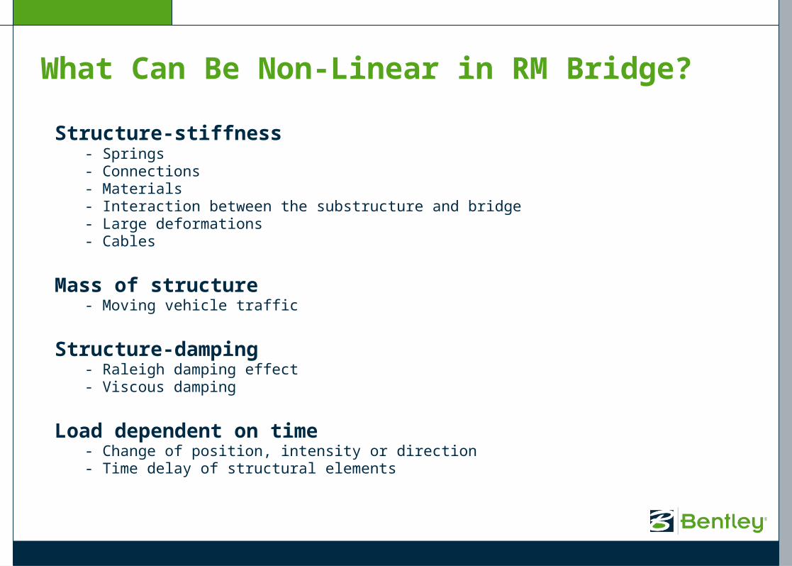
What Can Be Non-Linear in RM Bridge?
Structure-stiffness- Springs- Connections- Materials- Interaction between the substructure and bridge- Large deformations- Cables
Mass of structure- Moving vehicle traffic
Structure-damping- Raleigh damping effect- Viscous damping
Load dependent on time- Change of position, intensity or direction- Time delay of structural elements
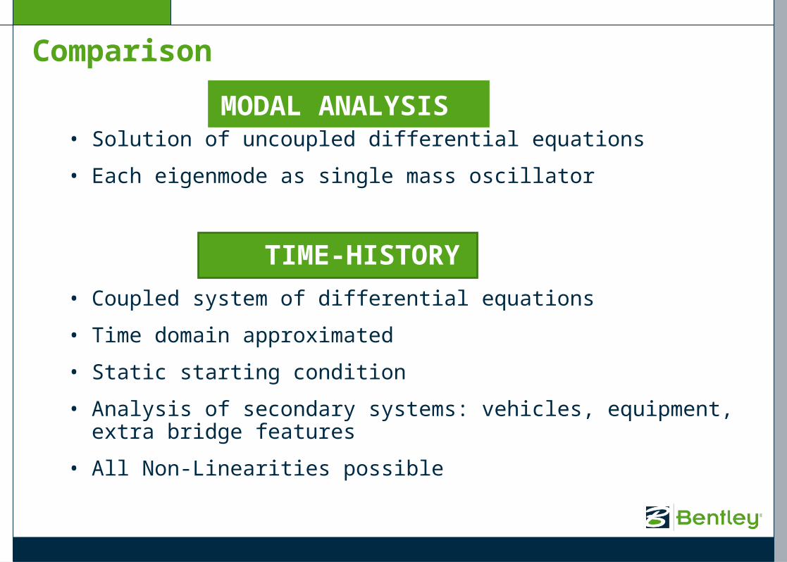
Comparison
• Solution of uncoupled differential equations
• Each eigenmode as single mass oscillator
• Coupled system of differential equations
• Time domain approximated
• Static starting condition
• Analysis of secondary systems: vehicles, equipment, extra bridge features
• All Non-Linearities possible
MODAL ANALYSIS
TIME-HISTORY
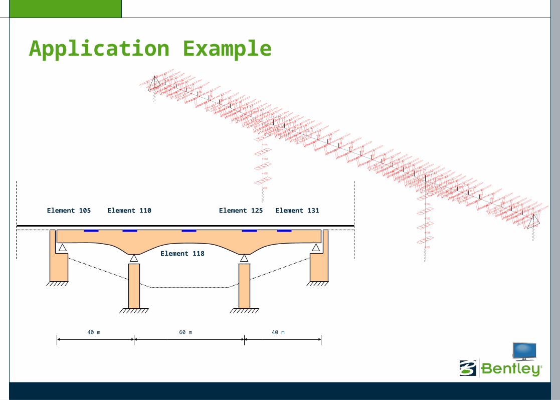
Element 105
40 m 60 m 40 m
Element 110
Element 118
Element 125 Element 131
Application Example

Bentley RM Bridge Seismic AnalysisConclusions
46 | WWW.BENTLEY.COM
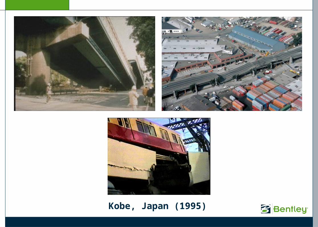
Kobe, Japan (1995)

48 | WWW.BENTLEY.COM
Akashi-Kaikyo – “Pearl Bridge”

RM Bridge Benefits
• Bentley BrIM vision
• Bentley portfolio
• Intuitive step-by-step calculation
• One tool for all: static, modal, time-history
• Integrated reports and drawings
Bentley RM Bridge Seismic Design and AnalysisQuestions
50 | WWW.BENTLEY.COM

Thank you for your [email protected]