www.elsevier.com/locate/marpolbul

Marine Pollution Bulletin 50 (2005) 264–275

Benthic diatom community response to environmental variablesand metal concentrations in a contaminated bay adjacent to

Casey Station, Antarctica

Laura Cunningham, Ian Snape, Jonathan S. Stark, Martin J. Riddle *

Human Impacts Research Program, Australian Antarctic Division, Channel Highway, Kingston, Tasmania 7050, Australia

Abstract

This study examined the effects of anthropogenic contaminants and environmental variables on the composition of benthic dia-

tom communities within a contaminated bay adjacent to an abandoned waste disposal site in Antarctica. The combination of geo-

graphical, environmental and chemical data included in the study explained all of the variation observed within the diatom

communities. The chemical data, particularly metal concentrations, explained 45.9% of variation in the diatom communities, once

the effects of grain-size and spatial structure had been excluded. Of the metals, tin explained the greatest proportion of variation in

the diatom communities (28%). Tin was very highly correlated (R2 > 0.95) with several other variables (copper, iron, lead, and sum

of metals), all of which explained similarly high proportions of total variation. Grain-size data explained 23% of variation once the

effects of spatial structure and the chemical data had been excluded. The pure spatial component explained only 1.8% of the total

variance. The study demonstrates that much of the compositional variability observed in the bay can be explained by concentrations

of metal contaminants.

Crown Copyright � 2004 Published by Elsevier Ltd. All rights reserved.

Keywords: Benthic diatoms; Community composition; Petroleum hydrocarbons; Metal contamination; Casey Station, Antarctica

1. Introduction

It is well established that high concentrations of somemetals can have toxic effects on diatoms (Fisher and

Frood, 1980). These effects include reduced photosyn-

thetic ability (Rijstenbil et al., 1994), reduced growth

rate (Cid et al., 1995), and the cessation or interruption

of cell division and deformation of the diatom frustule

(Dickman, 1998). Studies which examine the effects of

metal toxicity on diatoms are typically laboratory based

experiments involving either a single diatom species ex-posed to several metals at varying concentrations, or

0025-326X/$ - see front matter Crown Copyright � 2004 Published by Else

doi:10.1016/j.marpolbul.2004.10.012

* Corresponding author.

E-mail address: martin.riddle@aad.gov.au (M.J. Riddle).

several different diatom species exposed to varying con-

centrations of the one metal (Mason et al., 1995). Some

work of this nature has been undertaken with marinediatoms, however, this has almost exclusively involved

planktonic taxa (Payne and Price, 1999; Rijstenbil

et al., 1994). Estuarine and nearshore marine sediments

are major sinks for anthropogenic metal contamination,

it is therefore surprising that scant information is avail-

able on the toxicity of metals to benthic marine diatoms.

Petroleum hydrocarbons can also affect the composi-

tion of diatom communities. Compositional differences,with marked changes in the presence or absence of spe-

cies, have been observed between control communities

and those exposed to either light crude oil, or diesel

based oil-cuttings (Plante-Cuny et al., 1993). More sub-

tle compositional differences have also been recorded,

vier Ltd. All rights reserved.

L. Cunningham et al. / Marine Pollution Bulletin 50 (2005) 264–275 265

with pollution sensitive species inhibited, as a result of

hydrocarbon contamination (Morales-Los and Goutz,

1990). Typically, marine species are more sensitive to

hydrocarbon contamination than their freshwater coun-

terparts (Kusk, 1981). Despite this, there is little infor-

mation available regarding the impact of petroleumhydrocarbons on benthic marine diatoms.

The toxicity of anthropogenic contaminants to dia-

tom communities is dependant on a variety of factors

including light availability (Østgaard et al., 1984), salin-

ity (Eriksen et al., 2001), temperature (Cid et al., 1995)

and the presence of sea-ice (Siron et al., 1996). These

environmental variables differ dramatically between

the Antarctic environment and more temperate environ-ments. Despite this, few studies have assessed whether

diatom communities in Antarctica are affected by

anthropogenic contaminants even though contaminants

have been recorded around all Antarctic research sta-

tions so far examined (Kennicutt and McDonald,

1996). Detailed information about the extent of this con-

tamination, and resulting effects on biota are limited to

only a few sites, including McMurdo Station (Crockett,1997; Kennicutt et al., 1995), Signy Island (Cripps, 1992)

and Casey Station (Deprez et al., 1999; Snape et al.,

2001).

The marine environment around Casey Station, in

the Australian Antarctic Territory, has been contami-

nated with heavy metals and petroleum hydrocarbons.

Previous research has suggested these contaminants

may be influencing the diatom communities of marinebays immediately adjacent to this station (Cunningham,

2003; Cunningham et al., 2003). The purpose of this pa-

per was to assess the correlation between benthic diatom

communities and both anthropogenic contaminants and

other environmental variables in one of these contami-

nated bays. It was hypothesised that the anthropogenic

contamination would influence the diatom community

composition, and that the degree of disturbance to thediatom communities would be strongly correlated to

metal and/or hydrocarbon concentrations.

2. Site description

Casey Station is situated at 66�17 0 S, 110�32 0 E, on

Bailey Peninsula in the Windmill Islands, Antarctica(Fig. 1). It is the third permanent research station to

operate in the Windmill Islands. Its immediate predeces-

sor, �Old Casey� was also located on Bailey Peninsula,

approximately 800m northwest of the current Casey

Station. Approximately twenty sites in the immediate

vicinity of Casey and Old Casey Stations have been

identified as either contaminated, or potentially contam-

inated (Deprez et al., 1999). Documented contaminationevents include several fuels spills which have occurred in

the immediate area of these stations. In three separate

incidents between 1982 and 1999 more than 110,000 l

of Special Antarctic Blend (SAB) fuel leaked from

storage tanks, most of which entered the adjacent

marine environment (Deprez et al., 1999). In addition

to these large scale contamination events, smaller spills

associated with continuing operational activities havealso resulted in contaminants entering the Antarctic

environment.

Between 1969 and 1986 all refuse generated by the

Old Casey Station was dumped into the nearby Thala

Valley waste disposal site (Deprez et al., 1999) and occa-

sionally bulldozed onto the sea-ice in Brown Bay. The

dumped material included domestic and kitchen waste,

material from the various workshops, such as engineparts, batteries and old fuel drums, and waste from

the science laboratories and photographic darkroom

(Snape et al., 2001). Despite an earlier attempt to clean

up this site during the 1995–1996 summer season, it is

estimated that up to 2500m3 of rubbish and highly con-

taminated soil still remains (Snape et al., 2001).

The mobility of contaminants from these contami-

nated sites increases the potential for environmental im-pacts. Petroleum hydrocarbons have been traced from

the area surrounding the Old Casey mechanical work-

shop, through the Thala Valley catchment area, and into

the adjacent marine environment (Guille et al., 1997;

Cole et al., 2000). The processes responsible for this

movement have yet to be fully defined, however, both

surface run-off (Guille et al., 1997) and the movement

of groundwater (Cole et al., 2000) are implicated. Insummer, surface run-off flows through the Thala Valley

tip site where water dissolves and entrains contaminants

before discharging into the adjacent Brown Bay. An

estimated eight cubic meters of contaminated material

associated with the tip was removed by surface run-off

and deposited into Brown Bay during the 1998–1999

summer alone (Cole et al., 2000).

Metal concentrations (including Cu, Fe, Pb, Ag, Sn,Zn) in Brown Bay sediments are 10–100 times the con-

centrations in sediments from control locations (Snape

et al., 2001; Stark et al., 2003). Petroleum hydrocarbons,

derived from lubrication oil and Special Antarctic Blend

diesel fuel (SAB) are present in the surface sediments of

Brown Bay at concentrations ranging between 40 and

200mgkg�1 (unpublished data). In contrast, hydrocar-

bons that are unequivocally petroleum-derived contam-inants were not detected in sediments from control

locations (Snape et al., 2001).

Brown Bay is a small embayment aligned approxi-

mately east-west with rocky sides which grade to a rela-

tively homogenous muddy bottom (Stark, 2000). A

maximum depth of 20m occurs at the eastern end where

Brown Bay becomes part of Newcomb Bay. The Thala

Valley waste disposal site is located at the western endof the bay (Fig. 1) and waste material from the site is

widely dispersed over the floor of the bay.

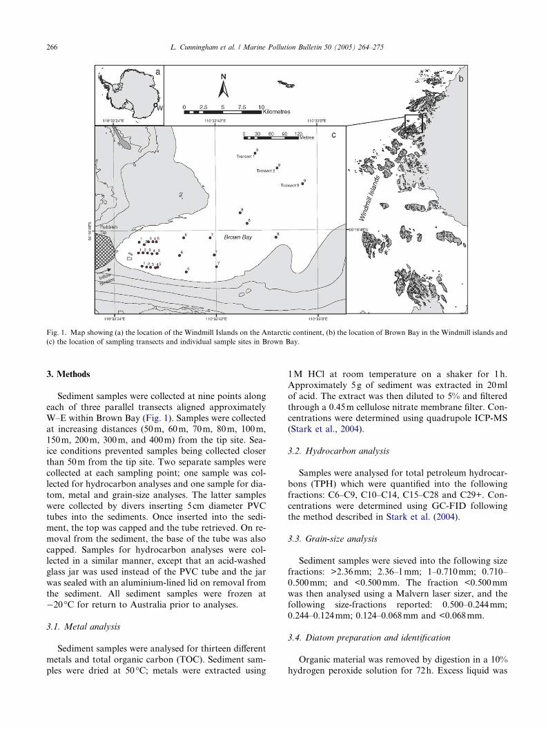
Fig. 1. Map showing (a) the location of the Windmill Islands on the Antarctic continent, (b) the location of Brown Bay in the Windmill islands and

(c) the location of sampling transects and individual sample sites in Brown Bay.

266 L. Cunningham et al. / Marine Pollution Bulletin 50 (2005) 264–275

3. Methods

Sediment samples were collected at nine points along

each of three parallel transects aligned approximately

W–E within Brown Bay (Fig. 1). Samples were collectedat increasing distances (50m, 60m, 70m, 80m, 100m,

150m, 200m, 300m, and 400m) from the tip site. Sea-

ice conditions prevented samples being collected closer

than 50m from the tip site. Two separate samples were

collected at each sampling point; one sample was col-

lected for hydrocarbon analyses and one sample for dia-

tom, metal and grain-size analyses. The latter samples

were collected by divers inserting 5cm diameter PVCtubes into the sediments. Once inserted into the sedi-

ment, the top was capped and the tube retrieved. On re-

moval from the sediment, the base of the tube was also

capped. Samples for hydrocarbon analyses were col-

lected in a similar manner, except that an acid-washed

glass jar was used instead of the PVC tube and the jar

was sealed with an aluminium-lined lid on removal from

the sediment. All sediment samples were frozen at�20 �C for return to Australia prior to analyses.

3.1. Metal analysis

Sediment samples were analysed for thirteen different

metals and total organic carbon (TOC). Sediment sam-

ples were dried at 50 �C; metals were extracted using

1M HCl at room temperature on a shaker for 1h.

Approximately 5g of sediment was extracted in 20ml

of acid. The extract was then diluted to 5% and filtered

through a 0.45m cellulose nitrate membrane filter. Con-

centrations were determined using quadrupole ICP-MS(Stark et al., 2004).

3.2. Hydrocarbon analysis

Samples were analysed for total petroleum hydrocar-

bons (TPH) which were quantified into the following

fractions: C6–C9, C10–C14, C15–C28 and C29+. Con-

centrations were determined using GC-FID followingthe method described in Stark et al. (2004).

3.3. Grain-size analysis

Sediment samples were sieved into the following size

fractions: >2.36mm; 2.36–1mm; 1–0.710mm; 0.710–

0.500mm; and <0.500mm. The fraction <0.500mm

was then analysed using a Malvern laser sizer, and thefollowing size-fractions reported: 0.500–0.244mm;

0.244–0.124mm; 0.124–0.068mm and <0.068mm.

3.4. Diatom preparation and identification

Organic material was removed by digestion in a 10%

hydrogen peroxide solution for 72h. Excess liquid was

L. Cunningham et al. / Marine Pollution Bulletin 50 (2005) 264–275 267

decanted, and the remaining slurry transferred to a cen-

trifuge tube. Distilled water was added so that the vol-

ume of each tube was 10ml. The samples were then

centrifuged for 5min at 3000rpm. The supernatant

was discarded, and the pellet was resuspended in dis-

tilled water (volume = 10ml). The centrifuging processwas repeated twice more. Following the third treatment,

the pellet was once again resuspended in distilled water.

This solution was diluted to approximately 10% and

pipetted onto coverslips. After air-drying, the coverslips

were mounted onto slides using Norland optical adhe-

sive 61 (Norland Products Inc., Cranberry, New Jersey).

Diatom valves were examined using a Zeiss KF2 light

microscope with 1000 · magnification, and phase con-trast illumination. Identification was primarily based

on Hasle and Syvertsen (1996), Roberts and McMinn

(1999) as well as Medlin and Priddle (1990). A minimum

of 400 individuals of the predominantly benthic taxa

was counted for each sample. The relative abundances

of these taxa were then calculated and used in the statis-

tical analyses. Only taxa which had a relative abundance

of 2% in at least one sample were included in the analy-sis. Exclusion of rare taxa was on the basis that they

may be allocthanous. For example, an exclusively fresh-

water species Luticola muticopsis (Van Heurck) Mann

was recorded in the sediment of Brown Bay, but was

probably derived from the meltstream that flows

through Thala Valley.

3.5. Statistical analysis

All of the chemical variables examined had skewed

distributions, and were therefore log (x + 1) transformed

prior to analysis. A detrended correspondence analysis

(DCA), detrending by segments, revealed the gradient

length of the ordination axis was less than 1, thus a lin-

ear response model was most applicable (ter Braak,

1987–1992). Redundancy analysis (RDA) was thereforeselected as the preferred ordination method. A prelimi-

nary ordination was used to determine the total varia-

tion explained by the spatial, chemical and grain-size

data. Multiple partitioning of variance (Borcard et al.,

1992) was used to assess the fraction of variance that

was explained by the chemical, grain-size and the spatial

data. This method also enables the amount of unex-

plained variation to be determined.The relationships between diatom data and the envi-

ronmental variables were assessed using RDA ordina-

tions. Multiple collinearity between variables was

examined using variance inflation factors (VIFs). Large

VIFs (>20) indicate that a variable is highly correlated

with other variables, and thus contributes little informa-

tion to the ordination (ter Braak, 1987–1992). Correla-

tion scores were used to determine which variableswere highly correlated (>0.90). Preliminary ordinations

revealed that high VIFs were common within the data

set, indicating that many variables were highly corre-

lated with each other. Further preliminary ordinations

were undertaken to select the combination of variables

that explained the greatest amount of the variation ob-

served in the species data while minimising multiple col-

linearity. In the final RDA this combination was used asactive variables, with the remaining variables incorpo-

rated as passive variables.

Intra-set correlations were used to examine the rela-

tive contribution of the environmental variables to the

separate ordination axis. The significance of the first

and second ordination axes were determined using

unrestricted Monte Carlo permutation tests (99

permutations).

4. Results

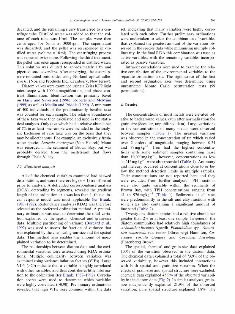
The concentrations of most metals were elevated rel-

ative to background values, even after normalisation for

grain-size (Scouller, unpublished data). Large variations

in the concentrations of many metals were observedbetween samples (Table 1). The greatest variation

was observed in the concentration of tin which varied

over 2 orders of magnitude, ranging between 0.24

and 37mgkg�1. Iron had the highest concentra-

tions with some sediment samples containing more

than 10,000mgkg�1, however, concentrations as low

as 216mgkg�1 were also recorded (Table 1). Antimony

and mercury occurred at concentrations close to or be-low the method detection limits in multiple samples.

Their concentrations are not reported here and they

were excluded from further analysis. TPH fractions

were also quite variable within the sediments of

Brown Bay, with TPH concentrations ranging from

41 to 976mgkg�1 (Table 1). Sediments at all sites

were predominantly in the silt and clay fractions with

some sites also containing a significant amount offine sand (Table 2).

Twenty one diatom species had a relative abundance

greater than 2% in at least one sample. In general, the

diatom communities had relatively high abundances of

Achnanthes brevipes Agardh, Planothidium spp., Stauro-

sira construens var. venter (Ehrenberg) Hamilton, Co-

cconeis costata Gregory and Cocconeis fasciolata

(Ehrenberg) Brown.The spatial, chemical and grain-size data explained

100% of the variation observed in the diatom data.

The chemical data explained a total of 73.9% of the ob-

served variability, however this included interactions

with both spatial and grain-size variables. When the

effects of grain-size and spatial structure were excluded,

chemical data explained 45.9% of the observed variabil-

ity in the diatom data (Fig. 2). In similar analyses, grain-size independently explained 21.9% of the observed

variation; pure spatial structure explained 1.8%. The

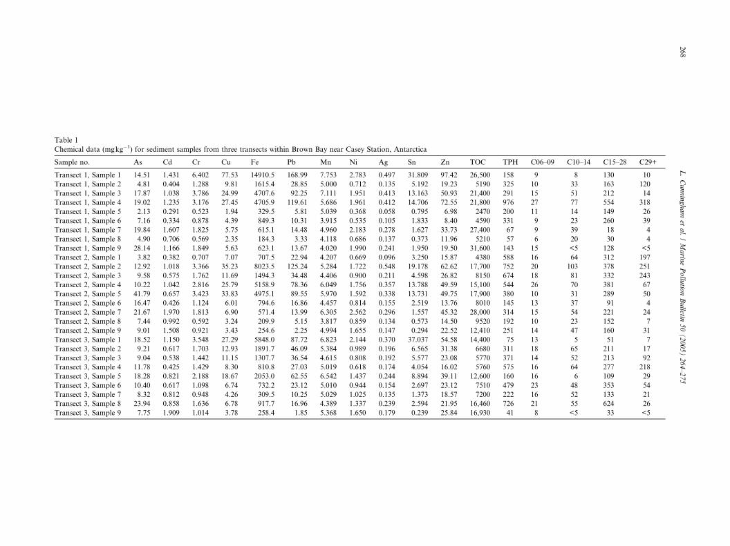
Table 1

Chemical data (mgkg�1) for sediment samples from three transects within Brown Bay near Casey Station, Antarctica

Sample no. As Cd Cr Cu Fe Pb Mn Ni Ag Sn Zn TOC TPH C06–09 C10–14 C15–28 C29+

Transect 1, Sample 1 14.51 1.431 6.402 77.53 14910.5 168.99 7.753 2.783 0.497 31.809 97.42 26,500 158 9 8 130 10

Transect 1, Sample 2 4.81 0.404 1.288 9.81 1615.4 28.85 5.000 0.712 0.135 5.192 19.23 5190 325 10 33 163 120

Transect 1, Sample 3 17.87 1.038 3.786 24.99 4707.6 92.25 7.111 1.951 0.413 13.163 50.93 21,400 291 15 51 212 14

Transect 1, Sample 4 19.02 1.235 3.176 27.45 4705.9 119.61 5.686 1.961 0.412 14.706 72.55 21,800 976 27 77 554 318

Transect 1, Sample 5 2.13 0.291 0.523 1.94 329.5 5.81 5.039 0.368 0.058 0.795 6.98 2470 200 11 14 149 26

Transect 1, Sample 6 7.16 0.334 0.878 4.39 849.3 10.31 3.915 0.535 0.105 1.833 8.40 4590 331 9 23 260 39

Transect 1, Sample 7 19.84 1.607 1.825 5.75 615.1 14.48 4.960 2.183 0.278 1.627 33.73 27,400 67 9 39 18 4

Transect 1, Sample 8 4.90 0.706 0.569 2.35 184.3 3.33 4.118 0.686 0.137 0.373 11.96 5210 57 6 20 30 4

Transect 1, Sample 9 28.14 1.166 1.849 5.63 623.1 13.67 4.020 1.990 0.241 1.950 19.50 31,600 143 15 <5 128 <5

Transect 2, Sample 1 3.82 0.382 0.707 7.07 707.5 22.94 4.207 0.669 0.096 3.250 15.87 4380 588 16 64 312 197

Transect 2, Sample 2 12.92 1.018 3.366 35.23 8023.5 125.24 5.284 1.722 0.548 19.178 62.62 17,700 752 20 103 378 251

Transect 2, Sample 3 9.58 0.575 1.762 11.69 1494.3 34.48 4.406 0.900 0.211 4.598 26.82 8150 674 18 81 332 243

Transect 2, Sample 4 10.22 1.042 2.816 25.79 5158.9 78.36 6.049 1.756 0.357 13.788 49.59 15,100 544 26 70 381 67

Transect 2, Sample 5 41.79 0.657 3.423 33.83 4975.1 89.55 5.970 1.592 0.338 13.731 49.75 17,900 380 10 31 289 50

Transect 2, Sample 6 16.47 0.426 1.124 6.01 794.6 16.86 4.457 0.814 0.155 2.519 13.76 8010 145 13 37 91 4

Transect 2, Sample 7 21.67 1.970 1.813 6.90 571.4 13.99 6.305 2.562 0.296 1.557 45.32 28,000 314 15 54 221 24

Transect 2, Sample 8 7.44 0.992 0.592 3.24 209.9 5.15 3.817 0.859 0.134 0.573 14.50 9520 192 10 23 152 7

Transect 2, Sample 9 9.01 1.508 0.921 3.43 254.6 2.25 4.994 1.655 0.147 0.294 22.52 12,410 251 14 47 160 31

Transect 3, Sample 1 18.52 1.150 3.548 27.29 5848.0 87.72 6.823 2.144 0.370 37.037 54.58 14,400 75 13 5 51 7

Transect 3, Sample 2 9.21 0.617 1.703 12.93 1891.7 46.09 5.384 0.989 0.196 6.565 31.38 6680 311 18 65 211 17

Transect 3, Sample 3 9.04 0.538 1.442 11.15 1307.7 36.54 4.615 0.808 0.192 5.577 23.08 5770 371 14 52 213 92

Transect 3, Sample 4 11.78 0.425 1.429 8.30 810.8 27.03 5.019 0.618 0.174 4.054 16.02 5760 575 16 64 277 218

Transect 3, Sample 5 18.28 0.821 2.188 18.67 2053.0 62.55 6.542 1.437 0.244 8.894 39.11 12,600 160 16 6 109 29

Transect 3, Sample 6 10.40 0.617 1.098 6.74 732.2 23.12 5.010 0.944 0.154 2.697 23.12 7510 479 23 48 353 54

Transect 3, Sample 7 8.32 0.812 0.948 4.26 309.5 10.25 5.029 1.025 0.135 1.373 18.57 7200 222 16 52 133 21

Transect 3, Sample 8 23.94 0.858 1.636 6.78 917.7 16.96 4.389 1.337 0.239 2.594 21.95 16,460 726 21 55 624 26

Transect 3, Sample 9 7.75 1.909 1.014 3.78 258.4 1.85 5.368 1.650 0.179 0.239 25.84 16,930 41 8 <5 33 <5

268

L.Cunningham

etal./Marin

ePollu

tionBulletin

50(2005)264–275

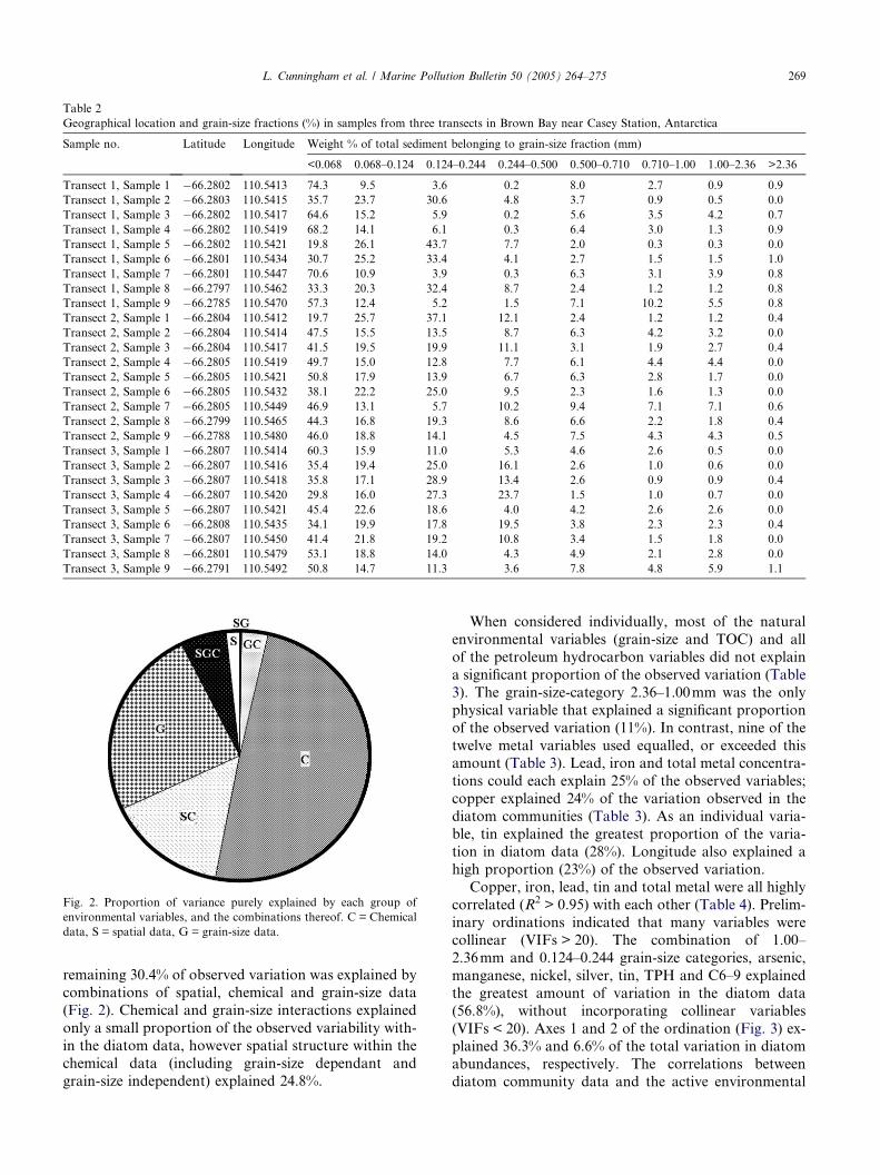
Table 2

Geographical location and grain-size fractions (%) in samples from three transects in Brown Bay near Casey Station, Antarctica

Sample no. Latitude Longitude Weight % of total sediment belonging to grain-size fraction (mm)

<0.068 0.068–0.124 0.124–0.244 0.244–0.500 0.500–0.710 0.710–1.00 1.00–2.36 >2.36

Transect 1, Sample 1 �66.2802 110.5413 74.3 9.5 3.6 0.2 8.0 2.7 0.9 0.9

Transect 1, Sample 2 �66.2803 110.5415 35.7 23.7 30.6 4.8 3.7 0.9 0.5 0.0

Transect 1, Sample 3 �66.2802 110.5417 64.6 15.2 5.9 0.2 5.6 3.5 4.2 0.7

Transect 1, Sample 4 �66.2802 110.5419 68.2 14.1 6.1 0.3 6.4 3.0 1.3 0.9

Transect 1, Sample 5 �66.2802 110.5421 19.8 26.1 43.7 7.7 2.0 0.3 0.3 0.0

Transect 1, Sample 6 �66.2801 110.5434 30.7 25.2 33.4 4.1 2.7 1.5 1.5 1.0

Transect 1, Sample 7 �66.2801 110.5447 70.6 10.9 3.9 0.3 6.3 3.1 3.9 0.8

Transect 1, Sample 8 �66.2797 110.5462 33.3 20.3 32.4 8.7 2.4 1.2 1.2 0.8

Transect 1, Sample 9 �66.2785 110.5470 57.3 12.4 5.2 1.5 7.1 10.2 5.5 0.8

Transect 2, Sample 1 �66.2804 110.5412 19.7 25.7 37.1 12.1 2.4 1.2 1.2 0.4

Transect 2, Sample 2 �66.2804 110.5414 47.5 15.5 13.5 8.7 6.3 4.2 3.2 0.0

Transect 2, Sample 3 �66.2804 110.5417 41.5 19.5 19.9 11.1 3.1 1.9 2.7 0.4

Transect 2, Sample 4 �66.2805 110.5419 49.7 15.0 12.8 7.7 6.1 4.4 4.4 0.0

Transect 2, Sample 5 �66.2805 110.5421 50.8 17.9 13.9 6.7 6.3 2.8 1.7 0.0

Transect 2, Sample 6 �66.2805 110.5432 38.1 22.2 25.0 9.5 2.3 1.6 1.3 0.0

Transect 2, Sample 7 �66.2805 110.5449 46.9 13.1 5.7 10.2 9.4 7.1 7.1 0.6

Transect 2, Sample 8 �66.2799 110.5465 44.3 16.8 19.3 8.6 6.6 2.2 1.8 0.4

Transect 2, Sample 9 �66.2788 110.5480 46.0 18.8 14.1 4.5 7.5 4.3 4.3 0.5

Transect 3, Sample 1 �66.2807 110.5414 60.3 15.9 11.0 5.3 4.6 2.6 0.5 0.0

Transect 3, Sample 2 �66.2807 110.5416 35.4 19.4 25.0 16.1 2.6 1.0 0.6 0.0

Transect 3, Sample 3 �66.2807 110.5418 35.8 17.1 28.9 13.4 2.6 0.9 0.9 0.4

Transect 3, Sample 4 �66.2807 110.5420 29.8 16.0 27.3 23.7 1.5 1.0 0.7 0.0

Transect 3, Sample 5 �66.2807 110.5421 45.4 22.6 18.6 4.0 4.2 2.6 2.6 0.0

Transect 3, Sample 6 �66.2808 110.5435 34.1 19.9 17.8 19.5 3.8 2.3 2.3 0.4

Transect 3, Sample 7 �66.2807 110.5450 41.4 21.8 19.2 10.8 3.4 1.5 1.8 0.0

Transect 3, Sample 8 �66.2801 110.5479 53.1 18.8 14.0 4.3 4.9 2.1 2.8 0.0

Transect 3, Sample 9 �66.2791 110.5492 50.8 14.7 11.3 3.6 7.8 4.8 5.9 1.1

Fig. 2. Proportion of variance purely explained by each group of

environmental variables, and the combinations thereof. C = Chemical

data, S = spatial data, G = grain-size data.

L. Cunningham et al. / Marine Pollution Bulletin 50 (2005) 264–275 269

remaining 30.4% of observed variation was explained by

combinations of spatial, chemical and grain-size data

(Fig. 2). Chemical and grain-size interactions explained

only a small proportion of the observed variability with-

in the diatom data, however spatial structure within the

chemical data (including grain-size dependant and

grain-size independent) explained 24.8%.

When considered individually, most of the natural

environmental variables (grain-size and TOC) and all

of the petroleum hydrocarbon variables did not explain

a significant proportion of the observed variation (Table

3). The grain-size-category 2.36–1.00mm was the only

physical variable that explained a significant proportion

of the observed variation (11%). In contrast, nine of the

twelve metal variables used equalled, or exceeded thisamount (Table 3). Lead, iron and total metal concentra-

tions could each explain 25% of the observed variables;

copper explained 24% of the variation observed in the

diatom communities (Table 3). As an individual varia-

ble, tin explained the greatest proportion of the varia-

tion in diatom data (28%). Longitude also explained a

high proportion (23%) of the observed variation.

Copper, iron, lead, tin and total metal were all highlycorrelated (R2 > 0.95) with each other (Table 4). Prelim-

inary ordinations indicated that many variables were

collinear (VIFs > 20). The combination of 1.00–

2.36mm and 0.124–0.244 grain-size categories, arsenic,

manganese, nickel, silver, tin, TPH and C6–9 explained

the greatest amount of variation in the diatom data

(56.8%), without incorporating collinear variables

(VIFs < 20). Axes 1 and 2 of the ordination (Fig. 3) ex-plained 36.3% and 6.6% of the total variation in diatom

abundances, respectively. The correlations between

diatom community data and the active environmental

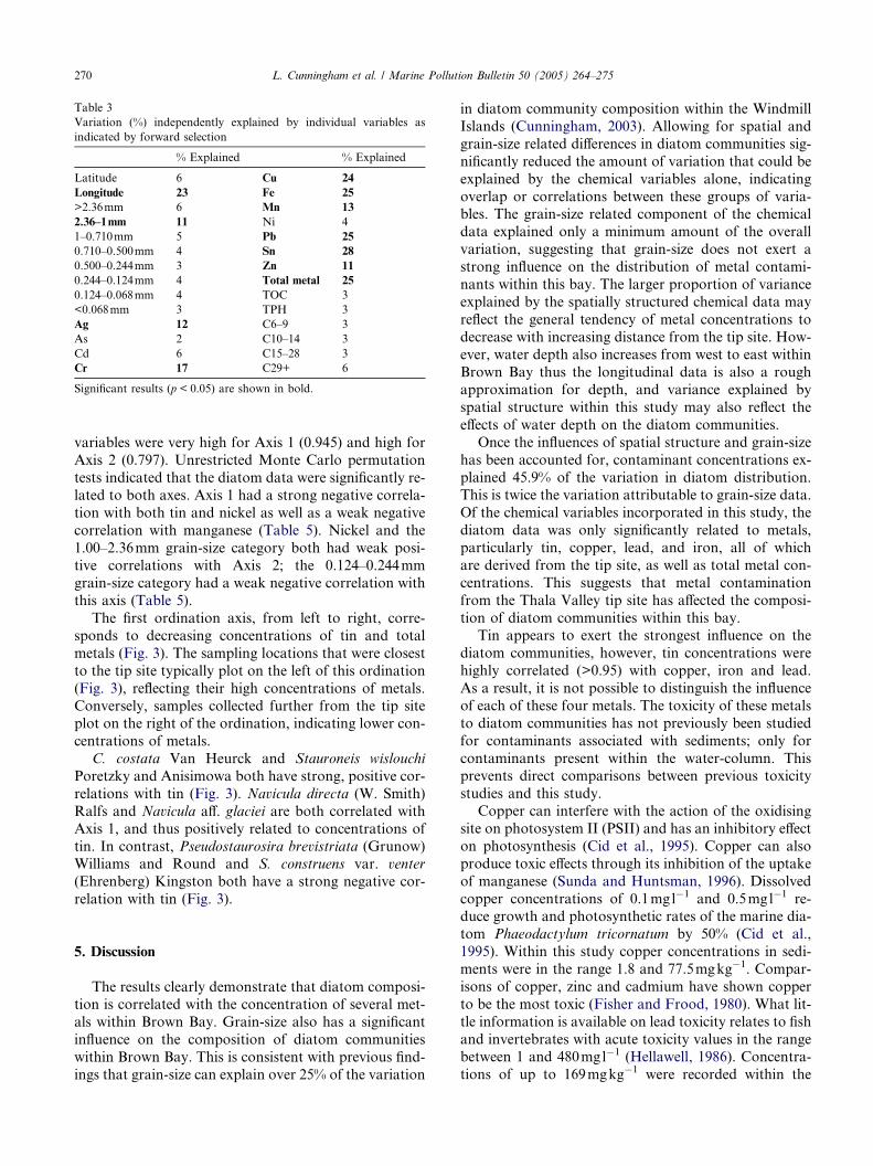
Table 3

Variation (%) independently explained by individual variables as

indicated by forward selection

% Explained % Explained

Latitude 6 Cu 24

Longitude 23 Fe 25

>2.36mm 6 Mn 13

2.36–1mm 11 Ni 4

1–0.710mm 5 Pb 25

0.710–0.500mm 4 Sn 28

0.500–0.244mm 3 Zn 11

0.244–0.124mm 4 Total metal 25

0.124–0.068mm 4 TOC 3

<0.068mm 3 TPH 3

Ag 12 C6–9 3

As 2 C10–14 3

Cd 6 C15–28 3

Cr 17 C29+ 6

Significant results (p < 0.05) are shown in bold.

270 L. Cunningham et al. / Marine Pollution Bulletin 50 (2005) 264–275

variables were very high for Axis 1 (0.945) and high for

Axis 2 (0.797). Unrestricted Monte Carlo permutation

tests indicated that the diatom data were significantly re-

lated to both axes. Axis 1 had a strong negative correla-

tion with both tin and nickel as well as a weak negative

correlation with manganese (Table 5). Nickel and the

1.00–2.36mm grain-size category both had weak posi-

tive correlations with Axis 2; the 0.124–0.244mmgrain-size category had a weak negative correlation with

this axis (Table 5).

The first ordination axis, from left to right, corre-

sponds to decreasing concentrations of tin and total

metals (Fig. 3). The sampling locations that were closest

to the tip site typically plot on the left of this ordination

(Fig. 3), reflecting their high concentrations of metals.

Conversely, samples collected further from the tip siteplot on the right of the ordination, indicating lower con-

centrations of metals.

C. costata Van Heurck and Stauroneis wislouchi

Poretzky and Anisimowa both have strong, positive cor-

relations with tin (Fig. 3). Navicula directa (W. Smith)

Ralfs and Navicula aff. glaciei are both correlated with

Axis 1, and thus positively related to concentrations of

tin. In contrast, Pseudostaurosira brevistriata (Grunow)Williams and Round and S. construens var. venter

(Ehrenberg) Kingston both have a strong negative cor-

relation with tin (Fig. 3).

5. Discussion

The results clearly demonstrate that diatom composi-tion is correlated with the concentration of several met-

als within Brown Bay. Grain-size also has a significant

influence on the composition of diatom communities

within Brown Bay. This is consistent with previous find-

ings that grain-size can explain over 25% of the variation

in diatom community composition within the Windmill

Islands (Cunningham, 2003). Allowing for spatial and

grain-size related differences in diatom communities sig-

nificantly reduced the amount of variation that could be

explained by the chemical variables alone, indicating

overlap or correlations between these groups of varia-bles. The grain-size related component of the chemical

data explained only a minimum amount of the overall

variation, suggesting that grain-size does not exert a

strong influence on the distribution of metal contami-

nants within this bay. The larger proportion of variance

explained by the spatially structured chemical data may

reflect the general tendency of metal concentrations to

decrease with increasing distance from the tip site. How-ever, water depth also increases from west to east within

Brown Bay thus the longitudinal data is also a rough

approximation for depth, and variance explained by

spatial structure within this study may also reflect the

effects of water depth on the diatom communities.

Once the influences of spatial structure and grain-size

has been accounted for, contaminant concentrations ex-

plained 45.9% of the variation in diatom distribution.This is twice the variation attributable to grain-size data.

Of the chemical variables incorporated in this study, the

diatom data was only significantly related to metals,

particularly tin, copper, lead, and iron, all of which

are derived from the tip site, as well as total metal con-

centrations. This suggests that metal contamination

from the Thala Valley tip site has affected the composi-

tion of diatom communities within this bay.Tin appears to exert the strongest influence on the

diatom communities, however, tin concentrations were

highly correlated (>0.95) with copper, iron and lead.

As a result, it is not possible to distinguish the influence

of each of these four metals. The toxicity of these metals

to diatom communities has not previously been studied

for contaminants associated with sediments; only for

contaminants present within the water-column. Thisprevents direct comparisons between previous toxicity

studies and this study.

Copper can interfere with the action of the oxidising

site on photosystem II (PSII) and has an inhibitory effect

on photosynthesis (Cid et al., 1995). Copper can also

produce toxic effects through its inhibition of the uptake

of manganese (Sunda and Huntsman, 1996). Dissolved

copper concentrations of 0.1mgl�1 and 0.5mgl�1 re-duce growth and photosynthetic rates of the marine dia-

tom Phaeodactylum tricornatum by 50% (Cid et al.,

1995). Within this study copper concentrations in sedi-

ments were in the range 1.8 and 77.5mgkg�1. Compar-

isons of copper, zinc and cadmium have shown copper

to be the most toxic (Fisher and Frood, 1980). What lit-

tle information is available on lead toxicity relates to fish

and invertebrates with acute toxicity values in the rangebetween 1 and 480mgl�1 (Hellawell, 1986). Concentra-

tions of up to 169mgkg�1 were recorded within the

Table 4

Correlations (R2) between variables, based on samples collected from Brown Bay adjacent to Casey Station, Antarctica

Longitude �0.72

GS8 �0.22 0.17

GS7 0.24 �0.12 �0.79

GS6 0.27 �0.16 �0.89 0.89

GS5 0.40 �0.09 �0.71 0.54 0.73

GS4 �0.43 0.36 0.78 �0.69 �0.82 �0.57

GS3 �0.51 0.40 0.67 �0.65 �0.78 �0.42 0.85

GS2 �0.46 0.54 0.45 �0.42 �0.57 �0.26 0.68 0.85

GS1 �0.55 0.38 0.29 �0.43 �0.43 �0.53 0.38 0.37 0.37

As 0.00 0.06 0.75 �0.57 �0.70 �0.37 0.53 0.62 0.42 0.00

Cd �0.43 0.47 0.76 �0.78 �0.84 �0.52 0.88 0.80 0.68 0.46 0.45

Cr 0.21 �0.45 0.73 �0.64 �0.68 �0.51 0.49 0.41 0.10 �0.02 0.66 0.39

Cu 0.39 �0.64 0.53 �0.44 �0.45 �0.33 0.32 0.22 �0.08 �0.16 0.50 0.18 0.94

Fe 0.41 �0.70 0.46 �0.35 �0.38 �0.33 0.23 0.15 �0.14 �0.20 0.45 0.06 0.92 0.97

Pb 0.56 �0.78 0.38 �0.30 �0.32 �0.22 0.11 0.06 �0.20 �0.28 0.46 �0.04 0.86 0.95 0.96

Mn 0.30 �0.40 0.51 �0.44 �0.53 �0.37 0.41 0.26 0.06 �0.10 0.38 0.43 0.78 0.73 0.68 0.62

Ni �0.21 0.11 0.88 �0.82 �0.94 �0.62 0.86 0.81 0.56 0.28 0.71 0.87 0.75 0.56 0.48 0.40 0.66

Ag 0.13 �0.32 0.76 �0.70 �0.73 �0.50 0.60 0.53 0.26 0.04 0.64 0.53 0.94 0.86 0.83 0.77 0.69 0.80

Sn 0.48 �0.74 0.42 �0.31 �0.32 �0.25 0.15 0.08 �0.24 �0.28 0.42 0.02 0.88 0.96 0.98 0.97 0.68 0.44 0.79

Zn 0.19 �0.32 0.76 �0.68 �0.73 �0.44 0.64 0.51 0.26 0.04 0.62 0.60 0.91 0.87 0.79 0.75 0.79 0.84 0.92 0.77

TOC �0.29 0.23 0.91 �0.83 �0.95 �0.63 0.87 0.87 0.66 0.31 0.81 0.84 0.69 0.48 0.40 0.33 0.48 0.95 0.76 0.34 0.76

TPH 0.39 �0.42 �0.19 0.18 0.16 0.26 �0.13 �0.12 �0.08 �0.31 0.05 �0.35 0.16 0.31 0.35 0.45 �0.06 �0.16 0.16 0.31 0.14 �0.11

C6�9 0.34 �0.27 0.07 �0.01 �0.10 0.18 0.03 0.18 0.17 �0.36 0.24 �0.03 0.26 0.33 0.35 0.46 0.14 0.14 0.29 0.36 0.33 0.15 0.74

C10�14 0.57 �0.40 �0.21 0.22 0.23 0.33 �0.27 �0.35 �0.16 �0.32 �0.09 �0.31 0.00 0.13 0.16 0.27 �0.06 �0.23 0.06 0.14 0.07 �0.24 0.71 0.47

C15�28 0.31 �0.33 �0.17 0.19 0.14 0.24 �0.05 �0.05 �0.04 �0.28 0.09 �0.32 0.18 0.31 0.35 0.42 �0.02 �0.13 0.16 0.31 0.13 �0.08 0.96 0.72 0.56

C29+ 0.55 �0.61 �0.32 0.30 0.33 0.32 �0.29 �0.35 �0.30 �0.34 �0.16 �0.43 0.11 0.33 0.36 0.45 0.03 �0.27 0.10 0.36 0.13 �0.31 0.86 0.54 0.75 0.73

Total metal 0.17 �0.65 0.48 �0.37 �0.39 �0.33 0.25 0.16 �0.13 �0.20 0.46 0.08 0.92 0.98 1.00 0.96 0.68 0.50 0.84 0.97 0.80 0.41 0.35 0.35 0.16 0.35 0.35

Latitude Longitude GS8 GS7 GS6 GS5 GS4 GS3 GS2 GS1 As Cd Cr Cu Fe Pb Mn Ni Ag Sn Zn TOC TPH C6–9 C10–14 C15–28 C29+

L.Cunningham

etal./Marin

ePollu

tionBulletin

50(2005)264–275

271

GS1

C4

GS3GS4

TOC

GS8

C15-28

Zn

Cr

CuMetalsPb

Fe C29+

C10-14

GS5

GS7

Lat

Long

GS3NiMn

TPH

Ag

Sn

AsC6-9

Axis 1A

xis

2

GS6

Axis 1

Axi

s 2

Achnanthesbrevipes

Trachyneisaspera

Cocconeisfasciolata

Pinnulariaquadratarea

Naviculasp.bStauroneiswislouchiiCocconeis costata

Naviculasp. aNaviculadirecta

Naviculaaff. glaciei

Achnanthessp. a

Planothidium spp.

CocconeispinnataNaviculasp. c

Amphora sp. c

Trigoniumarcticum

Cocconeis schuetti

Pseudostaurosirabrevistriata

Staurosiraconstruensvar. venter

Axis 1

Axi

s 2

2.42.3

1.4

1.7 1.9 2.7

2.93.9

2.83.41.3

2.5 2.1

1.5

3.7

3.81.8

3.6

2.6

1.6

1.1 3.51.2

3.1 2.23.3

3.2

(a) (b)

(c)

Fig. 3. Redundancy analysis (RDA) ordination of (a) environmental variables, (b) diatom species abundance, and (c) samples collected from Brown

Bay near Casey Station, Antarctica. The first numeral in the sample code (e.g., 2.4) represents the transect number (e.g., Transect 2) and the second

numeral represents the sample number (e.g., Sample 4) indicating the sample order in each transect, with samples numbers increasing with distance

from the tip site. Active environmental variables are shown in larger bold font; passive variables are shown in plain typeface.

272 L. Cunningham et al. / Marine Pollution Bulletin 50 (2005) 264–275

sediments of Brown Bay indicating the potential for bio-

logical impacts. Tin has previously been demonstratedto have toxic effects on diatoms at concentrations as

low as 0.04mgl�1 (Walsh et al., 1985); concentrations

reported in this study (up to 37.8mgkg�1). Insufficient

information exists regarding the toxicity of iron on

organisms for comparative assessments to be made.

Based on the available data, we cannot identify which

of these metals is causing the observed effect. The ob-

served relationship between diatom composition andtin may therefore result from the effects of copper, lead,

iron, tin, or a combination thereof.

Several contaminants explained similar percentages

of the variation within the diatom communities. Thiscan occur either when the distribution of several metals

is highly correlated, or when different metals have simi-

lar effects on the diatom communities. Antagonistic,

synergistic and over-additive responses have all been ob-

served when the toxic effects of two or more metals have

been examined. The metal pairs of copper–zinc, and

copper–cadmium both exhibit antagonism when applied

to the diatoms P. tricornatum and Skeletonema costa-

tum, clone Skel 0, decreasing the observed toxicity

(Braeck et al., 1980). In contrast, these metals acted in

Table 5

Intra-set correlations between active environmental variables and

ordination Axes 1 and 2

Axis 1 Axis 2

0.244–0.124mm 0.004 �0.516

2.36–1mm 0.414 0.544

As �0.083 0.315

Mn �0.511 0.481

Ni �0.770 0.553

Ag �0.492 0.397

Sn �0.819 0.205

TPH �0.170 0.219

C6–9 �0.108 0.362

Significant correlations are shown in bold.

L. Cunningham et al. / Marine Pollution Bulletin 50 (2005) 264–275 273

a synergistic manner when applied to the diatom Thalas-

siosira pseudonana, increasing the observed toxicity

(Braeck et al., 1980).The antagonism observed between metals is hypothe-

sised to result from competition for uptake sites (Braeck

et al., 1980). Manganese also competes with copper,

zinc, and cadmium for uptake sites in P. tricornatum

and it is likely that many divalent cations compete for

uptake via the same route in this species (Braeck et al.,

1980). Common uptake mechanisms have previously

been found in many different organisms (Braeck et al.,1980) and may explain why some divalent metals have

similar toxicological effects.

Compositional changes in benthic diatom communi-

ties resulting from metal contamination have previously

been documented in lakes (Ruggiu et al., 1998) and riv-

ers (Ivorra et al., 1999). Within our study, P. brevistriata

and S. construens var. venter had strong negative corre-

lations with metal concentrations, suggesting that thesespecies are sensitive to pollution. This is consistent with

previous reports of S. construens as pollution sensitive

(Ruggiu et al., 1998). The relative abundances of several

other species, including N. directa, N. aff. glaciei and

S. wislouchi, all increased with increasing concentrations

of tin, and associated metals, suggesting that these spe-

cies may be metal tolerant. Metal tolerance would

enable these species to compete more effectively andcapitalise on the reduced presence of pollution sensitive

species, thus increasing in abundance. The relative abun-

dances of these species may be of use in the assessment

of impacted sites elsewhere in Antarctica, however, it

would first be necessary to confirm that these responses

are consistently found at other locations and under a

range of contamination regimes.

It has previously been suggested that small algal spe-cies will become dominant in communities exposed to

chemical stress (Kinross et al., 1993). Increased abun-

dances of small forms of Navicula spp. have been related

to organic enrichment and eutrophication (Kelly and

Whitton, 1995) as well as zinc and cadmium pollution

(Ivorra et al., 1999). Within our study, abundances of

Navicula species did increase in conjunction with in-

creased metal concentrations, however this was true of

both large (N. directa) and small (N. aff. glaciei) species.

Furthermore, the relative abundances of other small

species, notably P. brevistriata and S. construens var.

venter decreased with increasing metal concentration.Our results do not support the suggestion that size is a

determining factor of sensitivity to pollutants.

The composition of benthic diatom communities

within Brown Bay is not strongly related to TPH con-

centrations. Measuring TPH, and fractions thereof, is

not sufficient to distinguish between naturally occurring

and anthropogenic hydrocarbons (Cripps and Priddle,

1991). TPH concentrations measured from two sedimentcores from a control location in the Windmill Islands,

ranged from <20mgkg�1 to 195mgkg�1 (unpublished

data). It is possible that the presence and variability

of these naturally occurring hydrocarbons may be mask-

ing any biological effects due to anthropogenic

contaminants.

A previous study in the Windmill Islands which used

experimental field manipulations to assess the impact ofanthropogenic contaminants found that both petroleum

hydrocarbon and metal contamination could signifi-

cantly affect the composition of benthic diatom commu-

nities recruiting to sediments, and that contamination by

petroleum hydrocarbons resulted in a comparatively lar-

ger effect (Cunningham et al., 2003). This contrasts with

the results of the current study, where hydrocarbons had

only a minimal effect. This could be because of the dif-ferent types of hydrocarbons involved. The previous

study applied petroleum hydrocarbons directly to the

sediments, to yield a mix of �200mgkg�1 SAB and

�200mgkg�1 lubrication oil. The current study exam-

ined total hydrocarbon concentrations, including the

natural diesel range organics, with concentrations in

the range 41–976mgkg�1. Metal concentrations also dif-

fer between the two studies; concentrations of tin andiron measured here are 20 times greater than in the

experimental study, and copper and zinc concentrations

are 3 times greater in the current study than were used in

the experiment.

Further comparisons between our findings and other

studies are hampered by a lack of published informa-

tion. This study is one of the first to assess the relation-

ship between sediment contamination and benthicmarine diatoms. Most previous studies examining the ef-

fects of contamination of benthic diatoms have assessed

responses to contaminants within the water-column and

not contaminants within the sediments itself. Further-

more, studies assessing the effects of contamination

on benthic species have typically looked at freshwater,

not marine, species (e.g. Ivorra et al., 1999; Ruggiu et

al., 1998). The pollution tolerances of estuarine andcoastal diatom species to pollution are essentially

unknown; data on this topic is so scarce it prevents

274 L. Cunningham et al. / Marine Pollution Bulletin 50 (2005) 264–275

the development of marine diatom indices for pollution

monitoring purposes (Sullivan, 1999).

Direct gradient techniques, such as those used in this

study, facilitate the development of transfer functions

which predict the value of an environmental variable

based on observed diatom community compositions.Diatom-based transfer functions have previously been

used to predict a variety of variables including water

depth (Campeau et al., 1999), salinity (Roberts and

McMinn, 1998; Juggins, 1992), pH (ter Braak and van

Dam, 1989) nutrients (Reavie and Smol, 2001) and chlo-

rophyll a (Jones and Juggins, 1995). The strong relation-

ships observed between the diatom abundances and

metal concentrations in this study indicate the feasibilityof using diatom data to predict metal concentrations

within this bay.

6. Conclusions

This study has demonstrated that the composition of

benthic diatom communities within Brown Bay is corre-lated with both grain-size and the distribution of

anthropogenic contaminants. The combination of these

variables explained a total of 100% of the variation ob-

served in the diatom communities. Chemical variables

explained 45.9% of the observed variation once the ef-

fects of spatial structure and grain-size had been ex-

cluded. A suite of metals consisting of tin, copper, lead

and iron were identified as the dominating influence onthe benthic diatom communities, although the individual

effects of these metals could not be distinguished. Benthic

diatoms have several advantages as biological indica-

tors–they have short generation times and so respond

quickly to environmental change; as phototrophs they

are found close to the sediment surface and are therefore

exposed to the sediment diffusion boundary layer; only

very small sediment samples are required to quantita-tively describe benthic diatom communities and, impor-

tantly, their frustules are preserved in the sediment where

they remain as a record of past environmental condi-

tions. Our data demonstrate that Antarctic marine bent-

hic diatoms are sensitive to a suite of anthropogenic

metals at concentrations that can occur as the result of

dispersion from terrestrial contaminated sites.

Acknowledgments

This work was carried out at the Institute of Antarc-

tic and Southern Ocean Studies and the Australian Ant-

arctic Division, with the financial support of a

Tasmanian University Strategic Scheme Scholarship

awarded to Laura Cunningham and an Australian Ant-arctic Division Ph.D. Scholarship awarded to Jonathan

S. Stark. Logistic support was provided by the Antarctic

Science Advisory Committee (ASAC Project No. 2201),

awarded to Martin J. Riddle.

Field support from Andrew Tabor, Paul Golds-

worthy and J. Davidson, provided through the Human

Impacts Program, Australian Antarctic Division, was

essential to this project, and is gratefully acknowledged.Preparation of samples for metal and hydrocarbon anal-

yses was undertaken by Scott Stark (AAD). Both the

metal and TOC analyses were performed by the Austral-

ian Government Analytical Laboratories, in Pymble,

NSW. TPH analyses were performed by technicians at

the Sandy Bay Laboratory of Analytical Services Tas-

mania. Identification of diatom species was improved

by the comments of M. Poulin.

References

Borcard, D., Legendre, P., Drapeau, P., 1992. Partialling out the

spatial component of ecological variation. Ecology 73 (3), 1045–

1055.

Braeck, G.S., Malnes, G., Jensen, A., 1980. Heavy metal tolerance of

marine phytoplankton. IV. Combined effects of zinc and cadmium

on growth and uptake in some marine diatoms. J. Exp. Mar. Biol.

Ecol. 42, 39–54.

Campeau, S., Pienitz, R., Hequette, A., 1999. Diatoms as quantitative

paleodepth indicators in coastal areas of the southern Beaufort Sea,

Arctic Ocean. Palaeogeogr. Palaeoclim. Palaeoecol. 146, 67–97.

Cid, A., Herrero, C., Torres, E., Abalde, J., 1995. Copper toxicity on

the marine microalga Phaeodactylum tricornatum: effects on pho-

tosynthesis and related parameters. Aquat. Toxicol. 31, 165–174.

Cole, C.M., Snape, I., Gore, D.B., Revill, A.T., Riddle, M.J., 2000.

Contaminants in the Antarctic III: chemical and physical processes

that influence contaminants in cold regions. In: Hughson, T.,

Ruckstuhl, C. (Eds.), ISCORD 2000: Proceedings of the Sixth

International Symposium on Cold Region Development. Office of

Antarctic Affairs, Hobart.

Cripps, G.C., 1992. The extent of hydrocarbon contamination in the

marine environment from a research station in the Antarctic. Mar.

Pollut. Bull. 25, 288–292.

Cripps, G.C., Priddle, J., 1991. Hydrocarbons in the Antarctic marine

environment. Antarctic Sci. 3 (3), 233–250.

Crockett, A.B., 1997. Water and wastewater quality monitoring,

McMurdo Station, Antarctica. Environ. Monit. Assess. 47, 39–57.

Cunningham, L., 2003. Benthic Diatom Communities of Coastal

Marine Environments of the Windmill Islands, Antarctica. PhD

thesis. University of Tasmania.

Cunningham, L., Stark, J.S., Snape, I., McMinn, A., Riddle, M.J.,

2003. Effects of metal and petroleum hydrocarbons on benthic

diatom communities near Casey Station, Antarctica: an experi-

mental approach. J. Phycol. 39, 490–503.

Deprez, P.P., Arens, M., Locher, H., 1999. Identification and

preliminary assessment of contaminated sites at Casey Station,

Wilkes Land, Antarctica. Polar Res. 35, 299–316.

Dickman, M., 1998. Benthic marine diatom deformities associated

with contaminated sediments in Hong Kong. Environ. Int. 24, 749–

759.

Eriksen, R.S., Mackey, D.J., van Dam, R., Nowak, B., 2001. Copper

speciation and toxicity in Macquarie Harbour, Tasmania: an

investigation using a copper ion selective electrode. Mar. Chem. 74,

99–113.

Fisher, N.S., Frood, D., 1980. Heavy metals and marine diatoms:

influence of dissolved organic compounds on the toxicity and

L. Cunningham et al. / Marine Pollution Bulletin 50 (2005) 264–275 275

selection for metal tolerance among four species. Mar. Biol. 59, 85–

93.

Guille, D., Revill, A., Bowman, J., 1997. Long-term Fate of Petroleum

Contaminants at Casey Station, Antarctica. CSIRO Marine

Research, Hobart.

Hasle, G.R., Syvertsen, E.E., 1996. Identifying marine diatoms. In:

Tomas, C.R. (Ed.), Identifying Marine Diatoms and Dinoflagel-

lates. Academic Press, Inc., Harcourt Brace & Company, New

York, pp. 5–385.

Hellawell, J.M., 1986. Biological Indicators of Freshwater Pollution

and Environmental Management. Elsevier Applied Science Pub-

lishers, London and New York.

Ivorra, N., Hettelaar, J., Tubbing, G.M.J., Kraak, M.H.S., Sabater, S.,

Admiraal, W., 1999. Translocation of microbenthic algal commu-

nities used for in situ analysis of metal pollution in rivers. Arch.

Environ. Contam. Toxicol. 37, 19–28.

Jones, V.J., Juggins, S., 1995. The construction of a diatom based

chlorophyll a transfer function and its application at three lakes on

Signy Island (maritime Antarctic) subject to differing degrees of

nutrient enrichment. Freshwater Biol. 34, 433–445.

Juggins, S., 1992. Diatoms in the Thames Estuary, England: ecology,

paleoecology and salinity transfer functionBibliotheca Diatomo-

logica, vol. 25. Cramer, Berlin, 216p.

Kelly, M.G., Whitton, B.A., 1995. The trophic diatom index: a new

index for monitoring eutrophication in rivers. J. Appl. Phycol. 7,

433–444.

Kennicutt, M.C., McDonald, S.J., 1996. Marine disturbance—con-

taminants. Antarctic Res. Ser. 70, 401–415.

Kennicutt, M.C., McDonald, S.J., Sericano, J.L., Boothe, P., Oliver,

J., Safe, S., Presley, B.J., Liu, H., Wolfe, D., Wade, T.L., Crockett,

A., Bockus, D., 1995. Human contamination of the marine

environment—Arthur Harbour and McMurdo Sound, Antarctica.

Environ. Sci. Technol. 29, 1279–1287.

Kinross, J.H., Christofi, N., Read, P.A., Harriman, R.A., 1993.

Filametous algal communities related to pH in streams in

Trossachs, Scotland. Freshwater Biol. 30, 301–317.

Kusk, K.O., 1981. Comparison of the effects of aromatic hydrocarbons

on a laboratory alga and natural phytoplankton. Bot. Mar. 24,

611–613.

Mason, R.P., Reinfelder, J.R., Morel, F.M.M., 1995. Uptake, toxicity

and trophic transfer of mercury in a coastal diatom. Environ. Sci.

Technol. 30, 1835–1845.

Medlin, L.K., Priddle, J. (Eds.), 1990. Polar Marine Diatoms. British

Antarctic Survey. Natural Environment Research Council, p. 214.

Morales-Los, M.R., Goutz, M., 1990. Effects of the water soluble

fraction of the Mexican crude oil ‘‘Isthmus Cactus’’ on growth,

cellular content of chlorophyll a and lipid composition of plank-

tonic microalgae. Mar. Biol. 104, 503–509.

Østgaard, K., Hegseth, E.N., Jensen, A., 1984. Species dependent

sensitivity of marine planktonic algae to Ekofisk crude oil under

different light conditions. Bot. Mar. XXVII, 309–318.

Payne, C.D., Price, N.M., 1999. Effects of cadmium toxicity on growth

and elemental composition of marine phytoplankton. J. Phycol. 35,

293–302.

Plante-Cuny, M.R., Salen-Picard, C., Grenz, G., Plante, R., Alliot, E.,

Barranguet, C., 1993. Experimental field study on the effects of

crude oil, drill cuttings and natural biodeposits on microphyto- and

macrozoobenthic communities in a Mediterranean area. Mar. Biol.

117, 355–366.

Reavie, E.D., Smol, J.P., 2001. Diatom-environmental relationships in

64 alkaline southeastern Ontario (Canada) lakes: a diatom-based

model for water quality reconstructions. J. Paleolimnol. 25 (1), 25–

42.

Rijstenbil, J.W., Sandee, A., Van Drie, J., Wijnholds, J.A., 1994.

Interaction of toxic trace metals and mechanisms of detoxification

in the planktonic diatoms Ditylum brightwellii and Thalassiosira

pseudonana. FEMS Microbiol. Rev. 14, 387–396.

Roberts, D., McMinn, A., 1998. A weighted-averaging regression and

calibration model for inferring lakewater salinity from fossil

diatom assemblages in the saline lakes of the Vestfold Hills:

implications for interpreting Holocene lake histories in Antarctica.

J. Paleolimnol. 19 (2), 99–113.

Roberts, D., McMinn, A., 1999. Diatoms of the saline lakes of the

Vestfold Hills, Antarctica. Bibl. Diatomologica 44, 1–83.

Ruggiu, D., Luglie, A., Cattaneo, A., Panzani, P., 1998. Paleoecolog-

ical evidence for diatom response to metal pollution in Lake Orta

(N. Italy). J. Paleolimnol. 20, 333–345.

Siron, R., Pelletier, E., Roy, S., 1996. Effects of dispersed and adsorbed

crude oil on microalgal and bacterial communities of cold seawater.

Ecotoxicology 5, 229–251.

Snape, I., Riddle, M.J., Stark, J.S., Cole, C.M., King, C.K., Duqense,

S., Gore, D.B., 2001. Management and remediation of contami-

nated sites at Casey Station, Antarctica. Polar Res. 37, 199–

214.

Stark, J.S., 2000. The distribution and abundance of soft-sediment

macrobenthos around Casey Station, East Antarctica. Polar Biol.

23, 840–850.

Stark, J.S., Riddle, M.J., Scouller, R.C., Snape, I., 2003. Human

impacts in Antarctic marine soft-sediment assemblages: correla-

tions between multivariate biological patterns and environmental

variables. Estuar. Coast. Shelf Sci. 56, 717–734.

Stark, J.S., Snape, I., Riddle, M.J., Stark, S.C., 2004. Constraints on

spatial variability in soft-sediment communities affected by con-

tamination from an antarctic waste disposal site. Mar. Pollut. Bull.

doi:10.1016/j.marpolbul.2004.10.015.

Sullivan, M.J., 1999. Applied diatom studies in estuaries and shallow

coastal environments. In: Stoermer, E.F., Smol, J.P. (Eds.), The

Diatoms: Applications for the Environmental and Earth Sciences.

Cambridge University Press.

Sunda, W.G., Huntsman, S.A., 1996. Antagonism between cadmium

and zinc toxicity and manganese limitation in a coastal diatom.

Limnol. Oceanogr. 41 (3), 373–387.

ter Braak, C.J.F., 1987–1992. CANOCO—a Fortran Program for

Canonical Community Ordination. Microcomputer Power, Ithaca,

NY, USA.

ter Braak, C.J.F., van Dam, H., 1989. Inferring pH from diatoms: a

comparison of old and new calibration models. Hydrobiologia 178,

209–223.

Walsh, G.E., McLaughlan, L.L., Lores, E.M., Louie, M.K., Deans,

C.H., 1985. Effects of organotins on growth and survival of two

marine diatoms, Skeletonema costatum and Thalassiosira pseudo-

nana. Chemosphere 14, 383–392.