-1

Benthic diatom communities as indicators of anthropogenic metal

contamination at Casey Station, Antarctica

Laura Cunningham, Ben Raymond, Ian Snape and Martin J. Riddle*Department of the Environment and Heritage, Australian Antarctic Division. Channel Highway, Kingston7050, Australia; *Author for correspondence (e-mail: martin.riddle@aad.gov.au)

Received 2 July 2003; accepted in revised form 9 January 2005

Key words: Antarctica, Diatoms, Diatom community composition, Marine pollution, Metal contamina-tion, MAT analysis, Paleo-reconstruction

Abstract

Prior to environmental legislation in the 1980s, anthropogenic waste in Antarctica was often deposited intolandfill sites or into the sea. This resulted in metal contamination in terrestrial and near-shore marineenvironments. In this study, we assess the feasibility of using both past and present diatom assemblages toreconstruct and monitor past and future metal contamination. Our dataset included the analyses of bothsurface sediment samples and sediment cores from a contaminated site near Casey Station, Antarctica.Redundancy analyses indicated a strong relationship between metal concentrations and the composition ofdiatom communities. Within the surface sediment samples, tin and lead individually explained 43% of thevariation observed in the diatom data; copper and iron explained 42% of this variation. In the sedimentcores, tin and lead individually explained 53% of the variation in diatom community composition. In thesame samples copper explained 47% of this variation, with iron explaining 46% of the observed variation.Once one metal had been selected, incorporating further metal data into the analyses added little extrainformation. Modern analog technique (MAT) analyses showed a strong correlation between actual andpredicted values within one dataset (R2: Cu 0.75; Pb 0.86; Sn 0.89; p<0.05 for each). MAT reconstructionsof metal concentrations closely followed measured concentrations, with both high and low concentrationsrecorded. MAT analyses performed favorably when compared to predictive techniques based on multi-variate linear regression and multilayer perceptron neural networks. This study demonstrates that thecomposition of benthic diatom communities is a good indicator of anthropogenic metal contamination, andmay be useful in monitoring the success of environmental remediation strategies in Antarctica and else-where.

Introduction

Diatoms are often ideal environmental indicators(Dixit et al. 1992). They are sensitive to environ-mental perturbations, and their short life cycleresults in rapid community response to environ-mental change (Sullivan 1999). The high preser-vation potential of diatoms means that they can

often be extracted from sediment cores to provideinformation about past diatom communities andthe environmental conditions under which thosecommunities grew (Dixit et al. 1992). Transferfunctions and modern analog techniques (MAT)permit quantitative estimates of past environ-mental conditions and are based on the modernrelationships between diatom community

Journal of Paleolimnology (2005) 33: 499–513 � Springer 2005

DOI 10.1007/s10933-005-0814-0

composition and environmental variables at anumber of representative sites. Such informationis especially important in Antarctica where thereare few historical environmental records. Diatom-based reconstructions have previously been usedto predict a variety of variables including surfacewater temperature (Zielinski et al. 1998; Bloomet al. 2003), water depth (Campeau et al. 1999),salinity (Sylvestre 2001; Roberts and McMinn1998), pH (ter Braak and Van Dam 1989; Siver etal. 2003), nutrients (Reavie and Smol 2001) andchlorophyll a (Jones and Juggins 1995). Envi-ronmental reconstructions are only feasible whendiatom community composition is stronglyrelated to the given environmental variable.

It has long been recognised that metal contam-ination can be toxic to diatoms (Braeck et al.1976). At a community level, the effects of metalcontamination are expressed as changes in speciescomposition, which can result in structural chan-ges such as decreased species diversity and richness(Crossey and La Point 1988). Compositionalchanges in benthic diatom communities resultingfrom metal contamination have been documentedin lakes (Ruggiu et al. 1998; Cattaneo et al. 2004)and rivers (Ivorra et al. 1999; Hirst et al. 2002;Griffith et al. 2002). Few studies have assessed theaffects of metal contamination on near-shoremarine diatom communities; the tolerances ofestuarine and coastal diatom species to pollutionare essentially unknown (Sullivan 1999). Giventhat estuarine and nearshore marine sediments aremajor sinks for anthropogenic metal contamina-tion, it is surprising that scant information isavailable on the toxicity of metals to benthicmarine diatoms.

Diatom communities in Brown Bay, a con-taminated marine inlet adjacent to Casey Stationin the Windmill Islands, East Antarctica, havebeen shown to be compositionally distinct fromother communities within the Windmill Islands(Cunningham 2003). This difference was attrib-uted both to environmental factors and toanthropogenic metal contamination (Cunningham2003). These studies demonstrated that sedimentmetal concentrations explained a large proportionof the variation in the composition of benthicdiatom communities, even when the effects ofgrain-size and location had been excluded. Of thechemical variables assessed, several metals (Cu,Fe, Pb and Sn) were found to have a major

influence on the diatom communities. However,the effects of the individual metals could not bedetermined due to the high correlations betweentheir concentrations in the sediments (Cunn-ingham 2003). A causal relationship betweenmetal concentrations and changes in diatomcommunity composition was also demonstrated(Cunningham et al. 2003) using experimentalmanipulations.

The primary goal of this study was to assess thefeasibility of using diatom communities in BrownBay to determine and monitor metal concentra-tions. If feasible, this method could then be appliedfor future monitoring and assessment work. Thefollowing two questions were addressed:

(1) Is the previously observed relationshipbetween diatom community composition andmetal concentrations maintained across abroad range of contaminant concentrations,and over time?

(2) Is this relationship strong enough to enable theprediction of metal concentrations?

Site description

The Windmill Islands cover an area of approxi-mately 75 km2 in Wilkes Land, Antarctica. CaseyStation is situated at 66�17¢ S, 110�32¢ E, on BaileyPeninsula in the Windmill Islands (Figure 1).Casey Station is the third permanent researchstation to operate in the Windmill Islands. Itsimmediate predecessor, ‘‘Old Casey’’, was alsolocated on Bailey Peninsula, approximately 800 mnorthwest of the current Casey Station. Between1969 and 1986 and before current environmentallegislation came into force, all waste generated atOld Casey Station, including waste from the sci-ence laboratories and various trade workshops aswell as domestically produced refuse was dumpedin the nearby Thala Valley (Snape et al. 2001).Accumulated waste was occasionally bull-dozedonto the sea-ice in Brown Bay (Deprez et al. 1999).During the 1995–1996 summer, an initial clean upof the Thala Valley waste disposal site wasundertaken. Although much of the rubbish wasremoved, it is estimated that 2500 m3 of tipmaterial and heavily contaminated soil remains(Snape et al. 2001).

500

Brown Bay is a small marine embayment ofNewcomb Bay, immediately adjacent to the ThalaValley waste disposal site. In summer, amelt-stream flows through the Thala Valley wastedisposal site where water dissolves and entrainscontaminants before discharging into Brown Bay(Figure 2). Four to eight cubic meters of contam-inated material associated with the waste disposalsite was removed by surface runoff and depositedinto Brown Bay during the 1998–1999 summerperiod alone (Cole et al. 2000). The concentrationsof some heavy metals and petroleum hydrocar-bons in sediments collected from Brown Bay havebeen found to be higher than those from controllocations. The concentrations of some metals,including copper, lead, iron and zinc, were 10 to100 times higher than background levels (Scoulleret al. 2000; Stark et al. 2003).

Brown Bay is aligned approximately west–eastand has a maximum depth of 20 m at the easternend where Brown Bay enters Newcomb Bay.Brown Bay has exposed rocky sides that grade to asediment-covered bottom consisting of relativelylarge patches of poorly mixed mud and fine sand,interspersed between gravel, cobbles and boulders

(Stark 2000). In addition, discarded tip material iswidely dispersed over the sea floor.

Methods

This study builds on previous research thatexamined the relationships between benthic dia-tom community composition and anthropogeniccontaminants within Brown Bay (Cunningham2003). Metal and diatom data from two previousstudies have been used here. The first study col-lected a series of samples along three west–easttransects through Brown Bay, in order to deter-mine contaminant concentrations and their effectson soft-sediment infauna (Stark et al. 2005). Thesecond study used several stratigraphic cores todetermine the temporal evolution of contaminantdeposition, and developed models for bioturbation(Snape et al., unpublished data).

The Brown Bay transect data included 27 ben-thic samples consisting of nine sampling points(50, 60, 70, 80, 100, 150, 200, 300, and 400 m fromthe Thala Valley waste disposal site) along threeparallel transects within Brown Bay (Figure 1).

Figure 1. Geographic location of Brown Bay including sampling sites. Sediment samples were collected from 9 points along each of 3

transects. In addition, six sediment cores were collected at varying distances from the Thala Valley tip site.

501

Samples were collected by divers inserting 20 cmlong, 5 cm diameter PVC tubes into the sediments.Once inserted into the sediment, the top was cap-ped and the tube retrieved. On removal from thesediment, the base of the tube was also capped. Allsediment samples were frozen at �20 �C for returnto Australia prior to analyses. After being dried at50 �C, each core was mixed individually and thesediments sub-sampled for both metal and diatomanalyses. This group of samples will subsequentlybe referred to as ‘‘transect samples’’.

Six stratigraphic cores were also collected fromwithin Brown Bay. Three of these cores werelocated close to the Thala Valley waste disposalsite, one core was from the middle of the bay, andthe remaining two cores from the outer regions ofBrown Bay (Figure 1). These cores were collectedby divers inserting 10 cm diameter PVC tubes intothe sediment. The top was then capped, the coreremoved, and the base of the core also capped.

These cores were then frozen at �20 �C and re-turned to Australia. These cores were sliced into2–3 mm sections, and sub-sampled for diatom,metal and 210Pb analyses. Some sections weresampled for all three types of analysis; these sam-ples will subsequently be referred to as ‘‘coresamples’’. Additional sections were analysed onlyfor diatom species composition and have beenincorporated into the latter stages of the recon-struction; these samples will be referred to as‘‘unknown metal’’ samples. Only samples frombelow the mixing layer within each core, as indi-cated by the 210 Pb profiles, were incorporated intothe statistical analyses. This was to remove anybias that may have resulted from comparing par-tially mixed sediments above this point to fullymixed sediments below it.

Metal analyses

Transect samples were dried at 50 �C; metals wereextracted using 1 M HCl at room temperature ona shaker for 1 hour. Approximately 1 g of sedi-ment was extracted in 20 ml of acid. The extractwas then diluted to 5% and filtered through a0.45 lm cellulose nitrate membrane filter. Metalconcentrations (Sb, As, Cd, Cu, Cr, Fe, Pb, Mn,Ni, Ag, Sn and Zn) were determined using highresolution Inductively Coupled Plasma-MassSpectrometry (ICP-MS).

Samples from the six additional sediment coreswere prepared for analysis using microwaveassisted acid digestion in hydrofluoric acid. Sam-ples were analysed for the same metals using eitherhigh resolution ICP-MS or Inductively CoupledPlasma-Atomic Emission Spectrometry (ICPAES).

210Pb analyses

Analyses of 210Pb were performed using alphaspectrometry. Isotopic ages were adjusted to allowfor sediment mixing.

Diatom preparation and identification

Excess organic material was removed by digestionin a 10% hydrogen peroxide solution for 72 hours.Excess liquid was decanted and the remaining

Figure 2. Aerial view of Brown Bay and surroundings, showing

the Thala Valley waste disposal site and the start of the sam-

pling transects.

502

slurry transferred to a centrifuge tube. Distilledwater was added so that the volume of each tubewas 10 ml. The samples were then centrifuged for5 min at 3000 rpm. The supernatant was decantedand the pellet was resuspended in 10 ml of distilledwater. The centrifuging process was repeated twicemore. Following the third treatment, the pellet wasonce again resuspended in distilled water. Thissolution was diluted to approximately 10% andpipetted onto coverslips. After air-drying, thecoverslips were mounted onto slides using Norlandoptical adhesive 61 (Norland Products Inc.,Cranberry, New Jersey).

Diatoms were examined using a Zeiss KF2 lightmicroscope with 1000· magnification and phasecontrast illumination. The diatom flora of marinebays of the Windmill Islands has been describedand illustrated in Cremer et al. (2003). Identifica-tion was primarily based on Hasle and Syvertsen(1996), Roberts and McMinn (1999) and Medlinand Priddle (1990). Species generally present onlywithin planktonic, or sea-ice communities wereexcluded from the data set. A minimum of 400valves of benthic species was counted for eachsample. The exact number of frustules countedvaried slightly between samples, with a maximumof 570 benthic diatoms counted in any one sample.The relative abundances of the benthic taxa werethen calculated and used in the statistical analyses.

Statistical analyses

Species were retained in numerical analyses if theyoccurred at abundances of >2% in at least threesamples, with at least one of these samples beingderived from each of the core samples and thesediment samples. No other transformations wereapplied to the diatom data. In addition to themeasured metal concentrations, the sum of allmetals was also calculated. All metal concentra-tions were log transformed prior to analysis. Thetransect and core data were analysed separatelydue to the different extraction methods used.

A preliminary detrended correspondence anal-ysis (DCA) was performed to determine whichtype of analysis was most appropriate for the data.Within both datasets the gradient lengths of thefirst four ordination axes were less than one stan-dard deviation, indicating that a linear responsemodel was most applicable (Ter Braak 1987–

1992). Variance partitioning (Borcard et al. 1992)was used to determine the amount of variancewithin the diatom communities that was due to themeasured metal variables and the amount due tothe location of sampling sites. The influence oflocation was assessed using the latitude and lon-gitude of the sampling sites after log(x+1) trans-formation. Redundancy analysis was used toexamine the relationships between diatom abun-dances and measured environmental variableswithin each dataset, and to determine which vari-ables were responsible for the variations observedin the diatom abundances. Forward selection wasused to determine the amount of variation thateach variable individually explained. The signifi-cance of each variable was tested using a MonteCarlo permutation test (with 99 permutations).

Constrained redundancy analysis (RDA) wasused to estimate the relative influence of indi-vidual variables in explaining the species data.The ratio of the eigenvalue of the first con-strained axis to the eigenvalue of the secondunconstrained axis was used to identify the rela-tive influence of the selected variable on the dia-tom data (Dixit et al. 1991). All ordinations wereperformed using the software package CANOCO(Ter Braak 1987–1992).

The MAT was applied to each dataset usingvariables that had a significant relationship withdiatom data, as indicated by the eigenvalue ratios.Analyses were initially performed using both themean of similar assemblages and the weightedmean of similar assemblages. Comparisons of theerror and the correlation between actual and pre-dicted values enabled the most accurate method tobe determined. All MAT analyses were performedusing C2 (Juggins 2003).

In order to assess the effectiveness of the MATtechnique, multivariate linear regression (MVL),and a multilayer perceptron neural network(MLPNN) using back propagation (Rumelhart etal. 1986) were also used to predict metal valuesfrom diatom assemblage data. These analyses wereperformed using MATLAB (Mathworks 2003).

Predictive abilities were estimated using ahold-out technique. One entire core or a singletransect sample was withheld from the trainingdata set, as each of these represented a discretesampling unit. The calculations for the MATmethod, or the model fitting for the other meth-ods, were carried out using the remaining data.

503

The values of the held-out core or transect samplewere then predicted and compared to actual val-ues. This process was then repeated but with adifferent core or transect sample left out, until eachcore and transect sample had been excluded inturn. This method avoids overly optimistic valuesfor prediction error, which can occur if the dataused for calculating prediction error are also usedfor model fitting.

MAT reconstructions (using the core samples asthe training set) were used to calculate likely con-centrations of Cu, Pb and Sn within the ‘‘unknownmetal’’ samples. These metals were selected for theMAT reconstructions because they all gave goodcorrelations (R2>0.75) between predicted andmeasured concentrations during the training stageof the MAT analysis.

Results

210Pb results indicated that the depth of the sedi-ment mixing layers of the core samples rangedbetween 0 and 30 mm. Forty seven core sampleswere analysed from below the mixing layer andthus incorporated into this study. A broad rangeof metal concentrations were recorded (Table 1)within the core samples, varying between back-ground concentrations to concentrations of 100times background. A number of metals, includingSn, had a bimodal distribution with few interme-diate values recorded. Cores 5 and 6 (which werefrom the outer regions of Brown Bay, Figure 1)had metal concentrations similar to backgroundlevels (Table 1). Metal concentrations in the coresamples were generally higher than those of thetransect samples, reflecting the more aggressiveextraction method used. Transect samples alsoshowed a range of contaminant concentrations,with both background and elevated concentrationsrecorded within these samples (Table 1). All con-centrations of Sb were at, or near, detection limitsand were therefore removed from further analyses.

Eleven diatom taxa occurred at abundancesgreater than 2% in at least one sample from bothtransect and core samples (Table 2). Hierarchicalclustering revealed a natural division of theassemblages into two groups. The first group wasdominated by Pseudostaurosira brevistriata andwith only low relative abundances of Naviculadirecta, Navicula sp. a, and Navicula sp. b. The

relative abundances of these species were moreevenly distributed within the second group. Sam-ples containing the first diatom assemblage hadrelatively low average concentrations of Sn(1.48 mg kg�1, interquartile range 1.0–1.7 mg kg�1)compared to samples containing the second dia-tom assemblage (16.91 mg kg�1, interquartilerange 10.8–35.0 mg kg�1). This relationship wasmaintained within both the core and transectsamples, suggesting that these groupings are con-sistent both spatially and temporally, regardless ofthe type of metal extraction method used.

A preliminary RDA ordination of the transectdata indicated that metal concentrations explained67.3% of the variation in diatom data (Figure 3),however this incorporated collinear variables(variance inflation factors >20). Variance parti-tioning indicated that 36% was due to metal con-centrations alone, with 31.3% due to thecombination of location and metal concentrations.A further 4.2% was explained by location alone,leaving 28.5% of total variation unexplained. Cu,Fe, Pb and Sn were very highly correlated(R2>0.90) with each other (Table 3). Each of thesevariables explained a high proportion of variationin the data, and was significantly related to thediatom data (Table 4). Cr, Ag and the sum of allmetals also explained significant proportions of theoverall variation (Table 4). As individual variables,Sn and Pb equally explained the highest proportionof the data (43%). The strong negative relationshipbetween metal concentrations and abundances ofPseudostaurosira brevistriata observed in the initialcluster analysis is also apparent on the spe-cies:environment biplot (Figure 3).

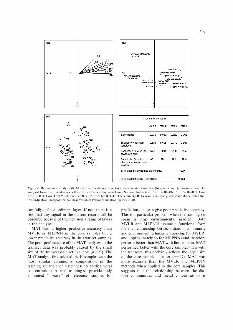
A preliminary RDA ordination of the core dataindicated that metal concentrations explained66.2% of the variation in diatom data (Figure 4).Variance partitioning revealed that 53.9% was dueto the metal component alone, with 12.7% due tothe location in combination with the metal data.Only 1.9% was explained by the location compo-nent alone, with the remaining 31.9% of variationin the diatom communities unexplained. Onceagain, Cu, Pb and Sn were very highly correlated(R2>0.90) with each other, however, correlationsbetween these metals and Fe decreased slightly(Table 3). As in the transect samples, each of thesevariables explained a high proportion of variationin the data, and were significantly related todiatom data (Table 4). As, Cr, Ag, Zn and the sum

504

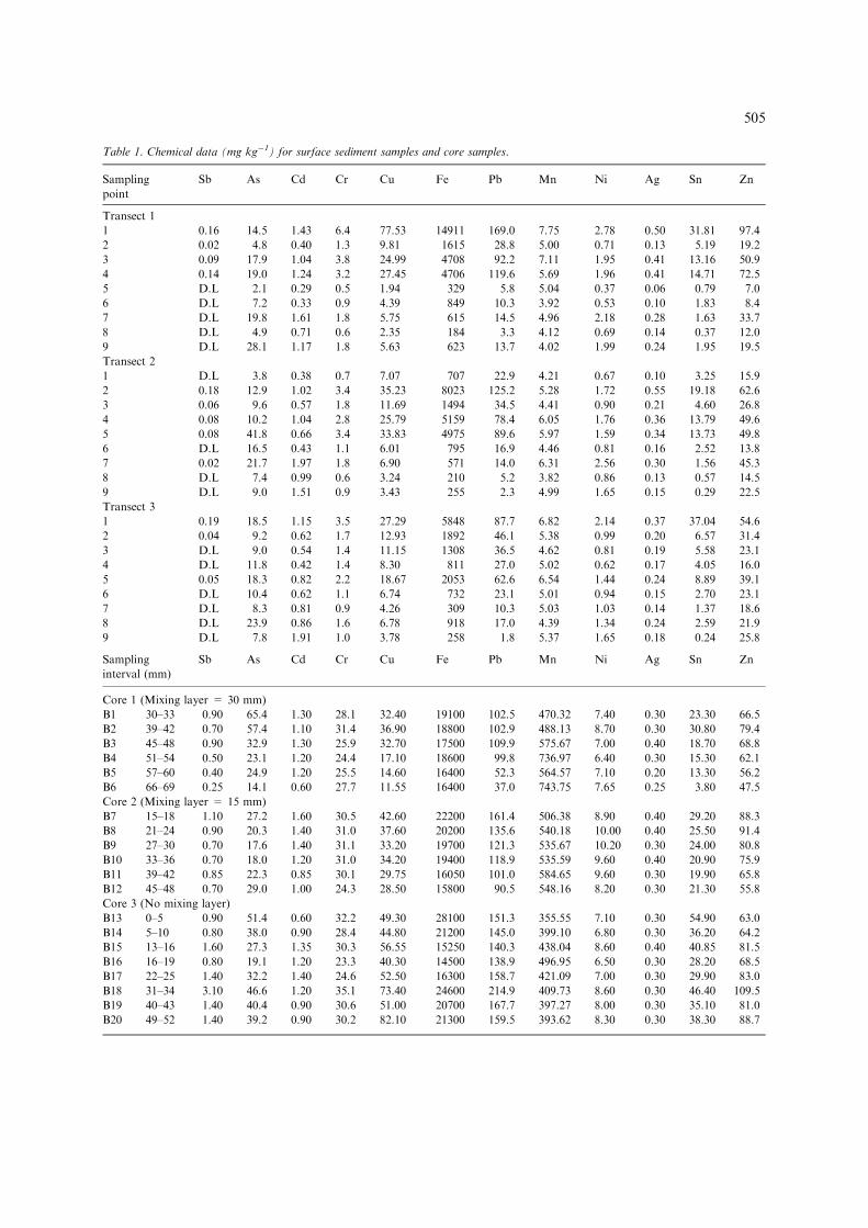
Table 1. Chemical data (mg kg�1) for surface sediment samples and core samples.

Sampling

point

Sb As Cd Cr Cu Fe Pb Mn Ni Ag Sn Zn

Transect 1

1 0.16 14.5 1.43 6.4 77.53 14911 169.0 7.75 2.78 0.50 31.81 97.4

2 0.02 4.8 0.40 1.3 9.81 1615 28.8 5.00 0.71 0.13 5.19 19.2

3 0.09 17.9 1.04 3.8 24.99 4708 92.2 7.11 1.95 0.41 13.16 50.9

4 0.14 19.0 1.24 3.2 27.45 4706 119.6 5.69 1.96 0.41 14.71 72.5

5 D.L 2.1 0.29 0.5 1.94 329 5.8 5.04 0.37 0.06 0.79 7.0

6 D.L 7.2 0.33 0.9 4.39 849 10.3 3.92 0.53 0.10 1.83 8.4

7 D.L 19.8 1.61 1.8 5.75 615 14.5 4.96 2.18 0.28 1.63 33.7

8 D.L 4.9 0.71 0.6 2.35 184 3.3 4.12 0.69 0.14 0.37 12.0

9 D.L 28.1 1.17 1.8 5.63 623 13.7 4.02 1.99 0.24 1.95 19.5

Transect 2

1 D.L 3.8 0.38 0.7 7.07 707 22.9 4.21 0.67 0.10 3.25 15.9

2 0.18 12.9 1.02 3.4 35.23 8023 125.2 5.28 1.72 0.55 19.18 62.6

3 0.06 9.6 0.57 1.8 11.69 1494 34.5 4.41 0.90 0.21 4.60 26.8

4 0.08 10.2 1.04 2.8 25.79 5159 78.4 6.05 1.76 0.36 13.79 49.6

5 0.08 41.8 0.66 3.4 33.83 4975 89.6 5.97 1.59 0.34 13.73 49.8

6 D.L 16.5 0.43 1.1 6.01 795 16.9 4.46 0.81 0.16 2.52 13.8

7 0.02 21.7 1.97 1.8 6.90 571 14.0 6.31 2.56 0.30 1.56 45.3

8 D.L 7.4 0.99 0.6 3.24 210 5.2 3.82 0.86 0.13 0.57 14.5

9 D.L 9.0 1.51 0.9 3.43 255 2.3 4.99 1.65 0.15 0.29 22.5

Transect 3

1 0.19 18.5 1.15 3.5 27.29 5848 87.7 6.82 2.14 0.37 37.04 54.6

2 0.04 9.2 0.62 1.7 12.93 1892 46.1 5.38 0.99 0.20 6.57 31.4

3 D.L 9.0 0.54 1.4 11.15 1308 36.5 4.62 0.81 0.19 5.58 23.1

4 D.L 11.8 0.42 1.4 8.30 811 27.0 5.02 0.62 0.17 4.05 16.0

5 0.05 18.3 0.82 2.2 18.67 2053 62.6 6.54 1.44 0.24 8.89 39.1

6 D.L 10.4 0.62 1.1 6.74 732 23.1 5.01 0.94 0.15 2.70 23.1

7 D.L 8.3 0.81 0.9 4.26 309 10.3 5.03 1.03 0.14 1.37 18.6

8 D.L 23.9 0.86 1.6 6.78 918 17.0 4.39 1.34 0.24 2.59 21.9

9 D.L 7.8 1.91 1.0 3.78 258 1.8 5.37 1.65 0.18 0.24 25.8

Sampling

interval (mm)

Sb As Cd Cr Cu Fe Pb Mn Ni Ag Sn Zn

Core 1 (Mixing layer = 30 mm)

B1 30–33 0.90 65.4 1.30 28.1 32.40 19100 102.5 470.32 7.40 0.30 23.30 66.5

B2 39–42 0.70 57.4 1.10 31.4 36.90 18800 102.9 488.13 8.70 0.30 30.80 79.4

B3 45–48 0.90 32.9 1.30 25.9 32.70 17500 109.9 575.67 7.00 0.40 18.70 68.8

B4 51–54 0.50 23.1 1.20 24.4 17.10 18600 99.8 736.97 6.40 0.30 15.30 62.1

B5 57–60 0.40 24.9 1.20 25.5 14.60 16400 52.3 564.57 7.10 0.20 13.30 56.2

B6 66–69 0.25 14.1 0.60 27.7 11.55 16400 37.0 743.75 7.65 0.25 3.80 47.5

Core 2 (Mixing layer = 15 mm)

B7 15–18 1.10 27.2 1.60 30.5 42.60 22200 161.4 506.38 8.90 0.40 29.20 88.3

B8 21–24 0.90 20.3 1.40 31.0 37.60 20200 135.6 540.18 10.00 0.40 25.50 91.4

B9 27–30 0.70 17.6 1.40 31.1 33.20 19700 121.3 535.67 10.20 0.30 24.00 80.8

B10 33–36 0.70 18.0 1.20 31.0 34.20 19400 118.9 535.59 9.60 0.40 20.90 75.9

B11 39–42 0.85 22.3 0.85 30.1 29.75 16050 101.0 584.65 9.60 0.30 19.90 65.8

B12 45–48 0.70 29.0 1.00 24.3 28.50 15800 90.5 548.16 8.20 0.30 21.30 55.8

Core 3 (No mixing layer)

B13 0–5 0.90 51.4 0.60 32.2 49.30 28100 151.3 355.55 7.10 0.30 54.90 63.0

B14 5–10 0.80 38.0 0.90 28.4 44.80 21200 145.0 399.10 6.80 0.30 36.20 64.2

B15 13–16 1.60 27.3 1.35 30.3 56.55 15250 140.3 438.04 8.60 0.40 40.85 81.5

B16 16–19 0.80 19.1 1.20 23.3 40.30 14500 138.9 496.95 6.50 0.30 28.20 68.5

B17 22–25 1.40 32.2 1.40 24.6 52.50 16300 158.7 421.09 7.00 0.30 29.90 83.0

B18 31–34 3.10 46.6 1.20 35.1 73.40 24600 214.9 409.73 8.60 0.30 46.40 109.5

B19 40–43 1.40 40.4 0.90 30.6 51.00 20700 167.7 397.27 8.00 0.30 35.10 81.0

B20 49–52 1.40 39.2 0.90 30.2 82.10 21300 159.5 393.62 8.30 0.30 38.30 88.7

505

of all metals also explained significant amounts ofvariation within the diatom communities(Table 4). Sn and Pb each explained 53% of the

variation within the diatom data, the highestproportion explained by any of the variables. Eachvariable explained a higher proportion of variationin the diatom data within the core samples thanwithin the transect samples (Table 4). Once againa strong negative relationship was observedbetween metal concentrations and the relativeabundance of Pseudostaurosira brevistriata(Figure 4).

MAT analyses were applied to Cr, Cu, Fe, Pb,Ag and Sn (Table 5) using both datasets. Withinthe transect samples, only Sn had a significantcorrelation between MAT-predicted and measuredvalues (P ¼ 0.05). Within the core samples, onlyAg did not show a significant correlation betweenMAT-predicted and measured values (Table 5).Strong correlations (R2>0.75) between MAT-predicted and measured values were observed forCu, Pb and Sn within the core samples (Table 5B).

Table 1. Continued

Sampling

interval (mm)

Sb As Cd Cr Cu Fe Pb Mn Ni Ag Sn Zn

B21 58–61 2.00 37.5 1.90 33.8 65.00 21800 190.0 450.19 9.40 0.50 39.40 122.9

Transect 1

B22 67–70 1.60 38.5 1.40 32.2 62.80 17500 170.4 419.06 9.60 0.30 34.90 125.3

B23 73–76 1.30 30.8 1.15 36.3 59.40 16500 144.7 495.05 10.70 0.30 27.00 118.0

B24 85–88 0.80 20.7 0.70 26.2 32.50 14500 117.4 611.21 10.40 0.30 16.90 80.7

Core 4 (No mixing layer)

B25 0–4 1.30 60.7 1.00 35.7 55.25 25300 157.0 457.79 14.29 0.90 34.00 86.3

B26 16–20 2.50 32.4 1.50 44.6 87.97 31700 189.0 418.90 18.13 1.10 50.80 150.7

B27 35–38 2.30 42.2 3.40 41.8 118.81 31500 232.0 439.69 14.47 1.10 51.10 282.5

B28 57–65 2.40 24.0 3.20 33.7 95.64 26300 190.0 529.99 12.74 1.40 37.40 217.7

Core 5 (mixing layer = 15 mm)

B29 15–18 D.L 25.8 1.70 23.5 14.80 11500 19.4 400.66 8.40 0.30 4.60 48.7

B30 21–24 D.L 13.5 1.20 21.5 10.30 12400 22.8 447.51 7.60 0.20 2.10 39.8

B31 27–30 D.L 11.2 1.20 20.0 8.50 12500 22.8 537.77 7.00 0.20 1.60 33.9

B32 36–39 D.L 10.9 1.20 20.8 12.90 12600 20.3 494.19 7.40 0.30 1.10 44.8

B33 45–48 D.L 9.9 1.30 22.2 9.80 12000 19.5 388.17 8.60 0.20 1.10 44.0

B34 51–54 D.L 11.7 1.40 23.4 10.00 12300 17.7 422.96 8.40 0.30 1.50 45.0

B35 57–60 D.L 9.4 1.30 21.0 8.80 12100 18.5 451.78 7.50 0.30 1.10 38.4

B36 63–66 D.L 11.0 1.40 26.4 11.10 11900 21.0 403.05 8.90 0.20 1.30 45.5

B37 69–72 D.L 7.2 1.70 21.7 9.20 12400 19.9 446.69 7.90 0.20 1.30 40.9

Core 6 (mixing layer = 12 mm)

B38 12–15 D.L 6.3 0.20 18.2 5.00 12700 28.7 712.86 5.30 0.20 1.70 23.6

B39 18–21 D.L 6.4 0.30 19.7 6.20 10850 30.4 614.51 5.55 0.25 1.70 25.2

B40 24–27 D.L 3.0 0.20 15.6 6.00 10600 27.7 613.32 4.60 D.L 1.10 25.1

B41 30–33 D.L 4.8 0.20 18.2 5.40 12100 29.5 754.74 5.30 D.L 1.40 24.2

B42 39–42 D.L 3.2 0.30 15.7 4.50 11800 26.5 702.30 4.30 D.L 1.20 22.3

B43 45–48 D.L 4.6 0.40 15.7 4.00 10100 28.3 531.07 4.60 D.L 1.00 22.5

B44 51–54 D.L 5.3 0.50 16.5 6.40 10400 25.7 570.32 5.00 D.L 0.90 26.3

B45 57–60 D.L 4.6 0.50 19.6 6.60 11300 27.7 600.60 6.20 D.L 1.00 32.6

B46 63–66 D.L 6.8 0.40 21.1 6.45 10550 28.5 543.69 6.55 D.L 0.80 37.4

B47 69–72 D.L 5.2 0.40 18.2 5.60 12100 25.9 587.89 5.60 D.L 0.90 30.5

D.L = detection limit.

Table 2. Species which occurred at relative abundances >2%in a minimum of three samples and which attained theseabundances in at least one recent sediment sample, and one coresample.

Species Name Authority (if applicable)

Achnanthes brevipes AgardhAchnanthes sp. a

Cocconeis costata/fasciolata

Navicula directa (W. Smith) RalfsNavicula sp. a

Navicula sp. b

Planothidium spp. Round and BuktiyarovaPseudostaurosira brevistriata (Grunow) Williams and RoundStaurosira construens var.venter

(Ehrenberg) Hamilton

Staurosira wislouchii Poretzky and AnisimowaTrachyneis aspera Ehrenberg

506

MAT analysis gave a better predictive accuracy formetal concentrations of core samples than eitherMVLR or the MLPNN. In contrast, MVLR andMLPNN had higher predictive accuracies for thetransect samples than the MAT analyses(Table 5A).

The neural network used was a multilayer per-ceptron neural network, which performs nonlinearregression. One hidden layer with two units wasused, which restricted the network to be onlyweakly nonlinear. Increasing the number of hiddenunits beyond two, and thus decreasing linearity,did not increase predictive accuracy. This suggeststhat the diatom-tin relationship is largely linear

and this is supported by the relatively good per-formance of multivariate linear regression. How-ever, it could also be caused by there being too fewdata for training the larger networks.

MAT analysis using the weighted mean of theten most similar assemblages was selected as thepreferred method as this generally resulted in ahigher correlation score (between actual and pre-dicted values) and a lower error value, than MATanalysis based on the unweighted mean of the tenmost similar assemblages. MAT reconstructionsusing the core samples as the training set wereapplied to the unknown metal samples to calculatelikely Cu, Pb and Sn concentrations. The resulting

Figure 3. Redundancy analysis (RDA) ordination diagrams of (a) environmental variables, (b) species and (c) surface sediment

samples collected from Brown Bay, near Casey Station, Antarctica. The first numeral in the sample code represents the transect

number and the second numeral indicates the sample order, with increasing numbers representing increasing distance from the tip site.

The summary RDA results are also given; it should be noted that this ordination incorporated collinear variables (variance inflation

factors >20).

507

values were generally similar to the measuredvalues of adjacent samples (Figure 5). The deepestsamples in Core 1 were an exception to this, with

calculated values higher than adjacent measuredvalues.

Discussion

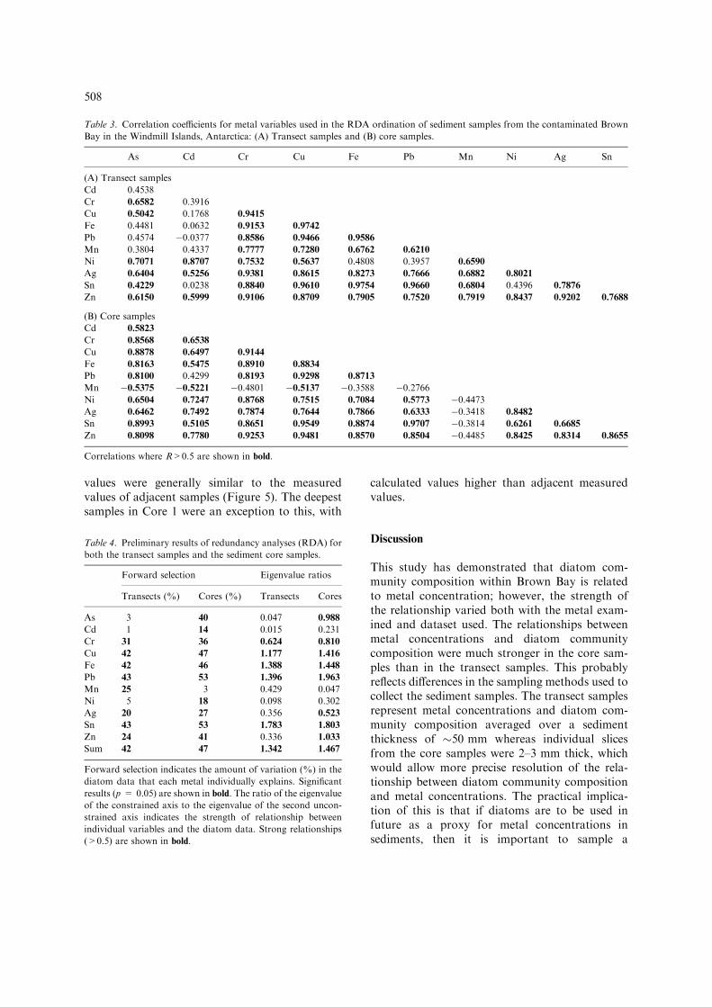
This study has demonstrated that diatom com-munity composition within Brown Bay is relatedto metal concentration; however, the strength ofthe relationship varied both with the metal exam-ined and dataset used. The relationships betweenmetal concentrations and diatom communitycomposition were much stronger in the core sam-ples than in the transect samples. This probablyreflects differences in the sampling methods used tocollect the sediment samples. The transect samplesrepresent metal concentrations and diatom com-munity composition averaged over a sedimentthickness of �50 mm whereas individual slicesfrom the core samples were 2–3 mm thick, whichwould allow more precise resolution of the rela-tionship between diatom community compositionand metal concentrations. The practical implica-tion of this is that if diatoms are to be used infuture as a proxy for metal concentrations insediments, then it is important to sample a

Table 3. Correlation coefficients for metal variables used in the RDA ordination of sediment samples from the contaminated Brown

Bay in the Windmill Islands, Antarctica: (A) Transect samples and (B) core samples.

As Cd Cr Cu Fe Pb Mn Ni Ag Sn

(A) Transect samples

Cd 0.4538

Cr 0.6582 0.3916

Cu 0.5042 0.1768 0.9415

Fe 0.4481 0.0632 0.9153 0.9742

Pb 0.4574 �0.0377 0.8586 0.9466 0.9586

Mn 0.3804 0.4337 0.7777 0.7280 0.6762 0.6210

Ni 0.7071 0.8707 0.7532 0.5637 0.4808 0.3957 0.6590

Ag 0.6404 0.5256 0.9381 0.8615 0.8273 0.7666 0.6882 0.8021

Sn 0.4229 0.0238 0.8840 0.9610 0.9754 0.9660 0.6804 0.4396 0.7876

Zn 0.6150 0.5999 0.9106 0.8709 0.7905 0.7520 0.7919 0.8437 0.9202 0.7688

(B) Core samples

Cd 0.5823

Cr 0.8568 0.6538

Cu 0.8878 0.6497 0.9144

Fe 0.8163 0.5475 0.8910 0.8834

Pb 0.8100 0.4299 0.8193 0.9298 0.8713

Mn �0.5375 �0.5221 �0.4801 �0.5137 �0.3588 �0.2766Ni 0.6504 0.7247 0.8768 0.7515 0.7084 0.5773 �0.4473Ag 0.6462 0.7492 0.7874 0.7644 0.7866 0.6333 �0.3418 0.8482

Sn 0.8993 0.5105 0.8651 0.9549 0.8874 0.9707 �0.3814 0.6261 0.6685

Zn 0.8098 0.7780 0.9253 0.9481 0.8570 0.8504 �0.4485 0.8425 0.8314 0.8655

Correlations where R>0.5 are shown in bold.

Table 4. Preliminary results of redundancy analyses (RDA) for

both the transect samples and the sediment core samples.

Forward selection Eigenvalue ratios

Transects (%) Cores (%) Transects Cores

As 3 40 0.047 0.988

Cd 1 14 0.015 0.231

Cr 31 36 0.624 0.810

Cu 42 47 1.177 1.416

Fe 42 46 1.388 1.448

Pb 43 53 1.396 1.963

Mn 25 3 0.429 0.047

Ni 5 18 0.098 0.302

Ag 20 27 0.356 0.523

Sn 43 53 1.783 1.803

Zn 24 41 0.336 1.033

Sum 42 47 1.342 1.467

Forward selection indicates the amount of variation (%) in the

diatom data that each metal individually explains. Significant

results (p = 0.05) are shown in bold. The ratio of the eigenvalue

of the constrained axis to the eigenvalue of the second uncon-

strained axis indicates the strength of relationship between

individual variables and the diatom data. Strong relationships

(>0.5) are shown in bold.

508

carefully defined sediment layer. If not, there is arisk that any signal in the diatom record will beobscured because of the inclusion a range of layersin the analyses.

MAT had a higher predictive accuracy thanMVLR or MLPNN in the core samples but alower predictive accuracy in the transect samples.The poor performance of the MAT analyses on thetransect data was probably caused by the smallsize of the transect data set available (n=27). TheMAT analysis first selected the 10 samples with themost similar community composition in thetraining set and then used these to predict metalconcentrations. A small training set provides onlya limited ‘‘library’’ of reference samples for

prediction, and can give poor predictive accuracy.This is a particular problem when the training setspans a large environmental gradient. BothMVLR and MLPNN assume a functional formfor the relationship between diatom communityand environment (a linear relationship for MVLR,and approximately so for MLPNN) and thereforeperform better than MAT with limited data. MATperformed better with the core samples than withthe transects; this probably reflects the larger sizeof the core sample data set (n=47). MAT wasmore accurate than the MVLR and MLPNNmethods when applied to the core samples. Thissuggests that the relationship between the dia-tom communities and metal concentrations is

Figure 4. Redundancy analysis (RDA) ordination diagrams of (a) environmental variables, (b) species and (c) sediment samples

analysed from 6 sediment cores collected from Brown Bay, near Casey Station, Antarctica. Core 1=B1–B6; Core 2=B7–B12; Core

3=B13–B24; Core 4=B25–28; Core 5=B29–37; Core 6=B38–47. The summary RDA results are also given; it should be noted that

this ordination incorporated collinear variables (variance inflation factors >20).

509

approximately linear but with some non-linearityover small scales. The MVLR and MLPNNmethods were able to capture the global linearity

but not the small-scale structure. MAT, whichessentially models only local structure, was betterable to capture the small-scale non-linearities. The

Table 5. Correlations and the root mean squared error (RMSE) between measured and predicted values for reconstruction of metal

concentrations in (A) transect and (B) core samples.

MAT WMAT MLP NN MVLR

R2 RMSE R2 RMSE R2 RMSE R2 RMSE

(A) Transect samples

Cr 0.328 0.141 0.293 0.144 0.379 0.136 0.388 0.141

Cu 0.482 0.261 0.480 0.260 0.608 0.229 0.623 0.238

Fe 0.471 0.385 0.445 0.389 0.667 0.303 0.661 0.324

Pb 0.459 0.368 0.449 0.368 0.530 0.360 0.507 0.399

Ag 0.216 0.038 0.179 0.038 0.181 0.038 0.244 0.040

Sn 0.536 0.297 0.538 0.292 0.616 0.270 0.622 0.284

(B) Core samples

Cr 0.601 0.069 0.600 0.069 0.356 0.088 0.304 0.094

Cu 0.751 0.022 0.756 0.023 0.552 0.273 0.557 0.271

Fe 0.682 0.078 0.684 0.08 0.556 0.091 0.503 0.099

Pb 0.864 0.143 0.881 0.133 0.653 0.229 0.627 0.238

Ag 0.344 0.066 0.380 0.065 0.280 0.071 0.334 0.069

Sn 0.888 0.19 0.891 0.187 0.827 0.234 0.769 0.270

Significant correlations (p=0.05) are shown in bold. Methods used are modern analog technique (MAT), weighted mean modern

analog technique (WMAT), multilayer perceptron neural network (MLPNN) and multivariate linear regression (MVLR). Predictive

values were calculated using a hold-out technique (see text).

Figure 5. Calculated (solid symbols) and measured (hollow symbols) values of copper (r), lead (n) and tin (m) in sequential layers

from sediment cores collected from the contaminated Brown Bay. Within each core the uppermost layer is on the left of the figure and

the bottom layer is to the right. Calculated concentrations are based on MAT analyses.

510

small scale signals would be retained in the coresample slices but tend to be smoothed out in thetransect data due to the depth of sediment(50 mm) used in these samples.

Metal concentrations, inferred using MAT, forthose layers in the cores that were not analysed,were generally very similar to the concentrationsmeasured in adjacent layers. Exceptions to thiswere the three deepest samples from Core 1, forwhich the adjacent measured metal concentrationdecreased to intermediate values, but the predictedvalues did not. This possibly reflects the bimodalnature of the metal data used as the training set,with the majority of samples having either high orlow concentrations of metals but few with inter-mediate concentrations.

The RDA analyses confirmed that diatomcommunity composition within Brown Bay isstrongly influenced by metal concentrations. Cu,Fe, Pb and Sn explained the majority of varianceattributable to metal concentrations, but were allhighly correlated. As a result it is impossible toaccurately distinguish the different effects of thesemetals. The observed relationship between diatomcomposition and Sn may therefore reflect the ef-fects of Cu, Pb, Sn, or a combination thereof.Similarly, predicted values of Sn may also reflectconcentrations of these other metals.

Grain-size data was not incorporated into thecurrent study because the aim of this study was toassess the feasibility of using diatom data alone asa proxy for measuring metal concentrations inBrown Bay. Water depth and the associated vari-able, ambient light intensity, are often cited as thedominant influences on diatom communities inAntarctica (e.g., Whitehead and McMinn 1997).However, location alone explained very little of thevariability within the diatom community of BrownBay despite there being a trend of increasing waterdepth from east to west along the transects. Onthis basis, water depth and light intensity have notbeen incorporated here.

Conclusions

This study demonstrated that metal concentra-tions, particularly those of Cu, Fe, Sn and Pbexplain a large proportion of variation in diatomcommunity composition observed within BrownBay. The observed correlation was consistent both

spatially and temporally in sediments from BrownBay. Although restricted by the size of the trainingset, this study has demonstrated the feasibility ofcalculating Sn (and associated metal) concentra-tions based on the composition of diatom com-munities within Brown Bay. The relationshipbetween metals and diatom communities wasstronger in the core samples than the transectsamples. This might have been an artefact of thesampling regimes (the core samples tended to showa bimodal distribution of tin, whereas the transectsamples were more evenly distributed betweenextremes). Alternatively, the relationship betweenmetals and diatom communities might be strongerwhen sampled at a fine scale by analysing thin(2–3 mm) sections of sediment than when largersamples, representing 100 mm or more of sedi-ment, are analysed. This is important for futuremonitoring work within the region, particularlywhere the objectives are to identify changes overrelatively short time frames, for example, to iden-tify environmental recovery after the source ofcontamination has been removed. Sampling of thetop 100 mm of sediment could obscure changes inrecent diatom communities that may be discernibleif only the surface layers were sampled. Techniqueswhich differentiate diatoms that are alive at thetime of sampling from dead diatom frustules pre-served in the sediments are important if the fine-scale relationship between environmental condi-tions and community composition are to be re-solved.

Acknowledgments

This work was carried out at the Institute ofAntarctic and Southern Ocean Studies, in con-junction with the Australian Antarctic Division,with the financial support of a Tasmanian Uni-versity Strategic Scheme Scholarship awarded toLaura Cunningham. Logistic support was pro-vided by Antarctic Science Advisory Committeegrants awarded to Martin J. Riddle (ASAC Pro-ject No. 2201). Dive support from Andrew Tabor,Paul Goldsworthy and Johnston Davidson, pro-vided through the Human Impacts Program,Australian Antarctic Division, was essential to thisproject, and is gratefully acknowledged. Diatomidentification was greatly assisted by the commentsof M. Poulin.

511

References

Bloom A.M., Moser K.A., Porinchu D.F. and McDonald G.M.

2003. Diatom-inference models for surface water temperature

and salinity developed from a 57 lake calibration set from the

Sierra Nevada, California, USA. J. Paleolimnol. 29: 235–255.

Borcard D., Legendre P. and Drapeau D. 1992. Partialling out

the spatial component of ecological variation. Ecology. 73:

1045–1053.

Braeck G.S., Jensen A. and Mohus A. 1976. Heavy metal tol-

erance of marine phytoplankton. IV. Combined effects of

copper and zinc on growth and uptake in cultures of four

common species. J. Exp. Mar. Biol. Ecol. 25: 37–54.

Campeau S., Pienitz R. and Hequette A. 1999. Diatoms as

quantitative paleodepth indicators in coastal areas of the

southern Beaufort Sea, Arctic Ocean. Palaeogeogr. Palaeoc-

lim. Palaeoecol. 146: 67–97.

Cattaneo A., Couillard Y., Wunsam S. and Courcells M. 2004.

Diatom taxonomic and morphological changes as indicators

of metal pollution and recovery in Lac Dufault (Quebec,

Canada). J. Paleolimnol 32: 163–175.

Cole C.M., Snape I., Gore D.B., Revill A.T. and Riddle M.J.

2000. Contaminants in the Antarctic Environment III:

Chemical and physical processes that influence contaminants

in cold regions. In: Hughson T. and Ruckstuhl C. (eds), IS-

CORD 2000: Proceedings of the Sixth International Sym-

posium on Cold Region Development. Office of Antarctic

Affairs, Hobart, pp. 128–131.

Cremer H., Roberts D., McMinn A., Gore D. and Melles M.

2003. The Holocene diatom flora of marine bays in the

Windmill Islands, East Antarctica. Bot. Mar. 46: 82–106.

Crossey M.J. and La Point T.W. 1988. A comparison of

periphyton community structure and functional responses to

heavy metals. Hydrobiol. 162: 109–121.

Cunningham L. 2003. Benthic diatom communities of coastal

marine environments in the Windmill Islands, Antarctica.

PhD Thesis, University of Tasmania.

Cunningham L., Stark J.S., Snape I., McMinn A. and Riddle

M.J. 2003. Effects of metal and petroleum hydrocarbons on

benthic diatom communities near Casey Station, Antarctica:

an experimental approach. J. Phycol. 39: 490–503.

Deprez P.P., Arens M. and Locher H. 1999. Identification and

preliminary assessment of contaminated sites at Casey Sta-

tion, Wilkes Land, Antarctica. Polar Rec. 35: 299–316.

Dixit S.S., Dixit A.S. and Smol J.P. 1991. Multivariable envi-

ronmental inferences based on diatom assemblages from

Sudbury Canada lakes. Freshwat. Biol. 26: 251–66.

Dixit S., Smol J.P., Kingston J.C. and Charles D.F. 1992.

Diatoms: powerful indicators of change. Environ. Sci.

Technol. 26: 23–33.

Griffith M.B., Hill B.H., Herhily A.T. and Kaufmann P.R.

2002. Multivariate analysis of periphyton assemblages in

relation to environmental gradients in the Colorado Rocky

Mountain Streams. J. Phycol. 38: 83–95.

Hasle G.R. and Syvertsen E.E. 1996. Identifying marine dia-

toms. In: Tomas C.R. (ed.), Identifying Marine Diatoms and

Dinoflagellates. Academic Press, Inc. Harcourt Brace &

Company, New York, pp. 5–385.

Hirst H., Juttner I. and Omerod S.J. 2002. Comparing the

responses of diatoms and macroinvertebrates to metals in

upland streams of Wales and Cornwall. Freshwater Biol. 47:

1752–1765.

Ivorra N., Hettelaar J., Tubbing G.M.J., Kraak M.H.S., Sa-

bater S. and Admiraal A. 1999. Translocation of microben-

thic algal communities used for in situ analysis of metal

pollution in rivers. Arch. Environ. Contam. Toxic. 37: 19–28.

Jones V.J. and Juggins S. 1995. The construction of a diatom

based chlorophyll a transfer function and its application at

three lakes on Signy Island (maritime Antarctic) subject to

differing degrees of nutrient enrichment. Freshwat. Biol. 34:

433–445.

Juggins S. 2003. C2 Software for ecological and palaeoecolog-

ical data analysis and visualization. University of Newcastle,

Newcastle upon Tyne, U.K.

Mathworks 2003. MATLAB. Mathworks Inc, Natick, Massa-

chusetts.

Medlin L.K. and Priddle J. (eds) 1990. Polar Marine Diatoms.

British Antarctic Survey, Natural Environment Research

Council, 214 pp.

Reavie E.D. and Smol J.P. 2001. Diatom-environmental rela-

tionships in 64 alkaline southeastern Ontario Canada lakes: a

diatom-based model for water quality reconstructions.

J. Paleolimnol. 25: 25–42.

Roberts D. and McMinn A. 1998. A weighted-averaging

regression and calibration model for inferring lakewater

salinity from fossil diatom assemblages in the saline lakes of

the Vestfold Hills: implications for interpreting Holocene

lake histories in Antarctica. J. Paleolimnol. 19: 99–113.

Roberts D. and McMinn A. 1999. Diatoms of the saline lakes

of the Vestfold Hills, Antarctica. Bibliotheca Diatomologica

44: 1–83.

Ruggiu D., Luglie A., Cattaneo A. and Panzani P. 1998.

Paleoecological evidence for diatom response to metal pol-

lution in Lake Orta (N. Italy). J. Paleolimnol. 20: 333–345.

Rumelhart D.E., Hinton G.E. and Williams R.J. 1986. Learn-

ing internal representations by error propagation. In: Parallel

Distributed Processing, vol. 1. MIT Press, Cambridge, MA,

pp. 318–362.

Scouller R.C., Stark J.S., Snape I., Riddle M.J. and Gore D.B.

2000. Contaminants in the Antarctic Environment V: Accu-

mulation in marine sediments. In: Hughson T. and Ruckstuhl

C. (eds), ISCORD 2000: Proceedings of the Sixth Interna-

tional Symposium on Cold Region Development. Office of

Antarctic Affairs, Hobart, pp. 136–139.

Siver P.A., Ricard R., Goodwin R. and Giblin A. 2003.

Estimating historical in-lake alkalinity generation from

sulfate reduction and its relationship to lake chemistry

as inferred from algal microfossils. J. Paleolimnol. 29:

179–197.

Snape I., Riddle M.J., Stark J.S., Cole C.M., King C.K.,

Duqense S. and Gore D.B. 2001. Management and remedi-

ation of contaminated sites at Casey Station, Antarctica.

Polar Rec. 37: 199–214.

Stark J.S. 2000. The distribution and abundance of soft-sedi-

ment macrobenthos around Casey Station, East Antarctica.

Polar Biol. 23: 840–850.

Stark J.S., RiddleM.J., Scouller R.C. and Snape I. 2003. Human

impacts in Antarctic marine soft-sediment assemblages: cor-

relations between multivariate biological patterns and envi-

ronmental variables. Estuar. Coast. Shelf Sci. 56: 717–734.

512

Stark J.S., Snape I., Riddle M.J., and Stark S.C. 2005. Con-

straints on spatial variability in soft-sediment communities

affected by contamination from an Antarctic waste disposal

site. Mar. Poll. Bull. 50: 276–290.

Sullivan M.J. 1999. Applied diatom studies in estuaries and

shallow coastal environments. In: Stoermer E.F. and Smol J.P.

(eds), The Diatoms: Applications for the Environmental and

Earth Sciences. Cambridge University Press, pp. 334–351.

Sylvestre F. 2001. Diatom-based ionic concentration and

salinity models from the south Bolivian Archipelago (15–23�S). J. Paleolimnol. 25: 279–295.

Ter Braak C.J.F. 1987–1992. Canoco – a Fortran program for

Canonical Community Ordination. Microcomputer Power

Ithaca, New York, USA.

Ter Braak C.J.F and van Dam H. 1989. Inferring pH from

diatoms: a comparison of old and new calibration models.

Hydrobiologia 178: 209–223.

Whitehead J. and McMinn A. 1997. Paleodepth determination

from Antarctic benthic diatom assemblages. Mar. Micropa-

leontol. 29: 301–308.

Zielinski U., Gersonde R., Sieger R. and Futterer D. 1998.

Quaternary surface water temperature estimations: calibra-

tion of a diatom transfer function for the Southern Ocean.

Paleoceanog. 13: 365–383.

513