1

Benefits of Government Bank Debt Guarantees:

Evidence from the Debt Guarantee Program

Jeffrey R. Black* jeff.black@ou.edu

Seth A. Hoelscher*

seth.hoelscher@ou.edu

Duane Stock** dstock@ou.edu

December 11, 2014

Finance Division Michael F. Price College of Business

University of Oklahoma 205A Adams Hall

Norman, OK 73019-0450

*University of Oklahoma ** Oklahoma Bankers Chair in Finance This paper was been nominated for a best investments paper award at the 2013 FMA (Chicago) meetings. Seth Hoelscher gratefully acknowledges financial support from the Center for Financial Studies and the Summer Research Paper support fund at the Michael F. Price College of Business. The authors greatly appreciate comments made during presentations at the FMA, University of Oklahoma, University of Maastricht, University of Leeds, and the Southwest Finance Symposium. The authors also appreciate comments and suggestions made by Louis Ederington, Pradeep Yadav, Vahap Uysal, Janya Golubeva, Marco Rossi, Stephanie Kleimeir, Thomas Post, Kevin Keasey, Paul Draper, Philip Holmes, John Polonchek, Matthew Crook, Tim Krehbiel, Alexey Malakhov, Peter Schotman, and Lisa Yang.

2

Benefits of Government Bank Debt Guarantees:

Evidence from the Debt Guarantee Program

Abstract

Bank liability guarantees have been an important tool to help stabilize banking systems for decades. Many aspects of design and effectiveness continue to be debated. How much, if any, should liability guarantees provide a subsidy to banks? Should weaker banks be permitted to enjoy greater subsidies? A bank bond insurance program executed in 2008 and 2009 provides a special opportunity to observe and measure bank benefits during a crisis period. The opportunity is especially rich because it presents an opportunity to observe how the term structure of credit spreads can be compared to a term structure of insurance premia charged. The relationship between the two term structures provides a potential template for the design of future bank liability insurance programs and also helps test alternative theories of corporate bond credit spreads. He and Xiong (2012), suggest credit spread slopes will tend to be negative during a crisis while, in contrast, Gorton, Metrick, and Xie (2014) suggest a positive slope. Our results support the former where this finding has very important implications for the design and effectiveness of insurance premia charged by bank liability insurers. We find that the term structure of the insurance premia charged enhanced the benefits that weaker banks received and may have helped to prevent bank failures. This finding is consistent with the theory that the liability insurance program meant to stabilize the financial system was designed in the spirit of those who feared a financial accelerator effect could have led to an even more severe economic downturn.

3

I. Introduction

In order for a banking system to function well, both borrowers and lenders must be

confident that the individual banks and, in general, the system are stable and ongoing. In

order to provide a stable banking system, it is very common to provide guarantees

(insurance) to those who provide funds to banks. The best known type of liability

guarantee in many countries is deposit insurance. Demirguc-Kunt and Huizinga (2004)

provide a description of deposit insurance systems of various countries. In the United

States, the deposit insurance system was instituted in 1933 to prevent depositor runs.

The optimal design of bank liability guarantees has been debated for decades and will

likely be debated for more decades given the complexity of design issues related to the

degree of subsidy regulators and politician choose to tolerate, unpredictability of crises,

and interactions with banking regulations that frequently change. A long list of questions

has been raised. Should banks pay the full fair market price for the guarantees? Is the

banking system sufficiently transparent to make full market pricing of guarantees

acceptable? If full market pricing is not applied, due to a financial crisis or other

complicating macroeconomic conditions, how much subsidy should banks receive when

they underpay? 1 How can the guarantee system prevent, or at least discourage, moral

hazard wherein banks acquire (overly) risky assets given the safe haven provided by a

guarantee.2

1 Arping (2009) maintains that fair pricing of guarantees are desirable only if the banking sector is sufficiently transparent. 2 Gropp, Gruendl, and Guettler (2013) show that government guarantees for German savings banks, which halted in 2001, were linked to substantial moral hazards.

4

Relatedly, many economists, politicians and policy makers maintain that banks with

relatively weak balance sheets and lower profitability (low credit quality) should pay more

for guarantees than stronger banks. If so, how much more should weaker banks pay and

how should the differential payment for guarantees be determined? 3 How can guarantees

be structured such that banks, especially large ones, will not be led to expect they will

always be bailed out during stressful periods? How much does the credit quality of the

sovereignty providing the guarantee affect the credibility of the guarantee? Should the level

of accumulated reserves in the deposit insurance fund help determine how much to charge

for guarantees? 4

Most of the dollar volume of liability guarantees has been in the form of deposit

insurance guarantees in the United States, as in many countries. Furthermore, most of the

economic research in regard to bank liability guarantees analyzes deposit insurance.

However, there has also been a significant volume of insured bank bonds (unsecured non-

deposit liabilities) in the early part of this century and only a limited amount of research

focuses upon insurance of bank bond issues wherein a government agency (or the

sovereignty itself) stands ready to pay off bond holders in case of bank failure. The same

questions posed above apply but, fortunately, there is much more evidence of the market

pricing of the value of the guarantee because the guaranteed instruments are publicly

traded and yields can easily be compared to comparable non-insured bonds of the same

bank.

3 Of course, differential payments may well result in differential subsidies that some may view as unfair aid to poorly managed banks. 4 If the reserves are low, perhaps the charge for guarantees should be increased.

5

The purpose of this research is to answer a myriad of important questions about

liability guarantees that regulators, policy makers, politicians, bank stockholders, bank

bondholders, and banker management would like answered. The first set of questions

concerns the liquidity provided by liability guarantee programs. We note that liquidity has

a myriad of definitions where, in our case, we focus upon microstructure measures of

liquidity for the bonds of particular bank.5 Do bonds that are insured enjoy greater

microstructure liquidity and thus permit banks to issue insured bonds at a lesser liquidity

premium and thus enjoy lower interest costs? If so, how much more liquid are insured

bonds versus non-insured bonds? Do non-insured bonds of the issuing firm realize an

improvement in liquidity when insured bonds are issued, or, on the other hand, does the

appeal of the insured bonds in effect reduce the demand for and the liquidity of uninsured

bonds of the same firm? We frame our answers to these questions in terms of literature

regarding flight to quality and flight to liquidity. In brief, bond insurance programs may be

less effective in reducing bond interest costs if bond investors are more concerned with

liquidity than quality. That is, instead of flocking to insured bank bonds, bond investors

may seek the high liquidity of U. S. Treasury bonds.

The second set of questions addresses how the theory and empirical research on the

term structure of credit spreads should affect the design of insurance premia term

structure. 6 This is very fundamental because the difference between the change in credit

5 As an example of other banking industry liquidity measures, the Basel Committee has recommended that banks report the relation of a particular bank’s volume of high quality liquid assets to expected net cash outflows for the next 30 days. The higher this ratio, the better a bank can withstand deposit runs and other liquidity crises. 6 Of course, conservative critics of such government intervention likely maintain that any possible undercharging is an unnecessary subsidy (gift) to banks, which is effectively corporate welfare. Any subsidization is also an important issue given any present and potential future FDIC financial distress of the

6

spread due to insurance purchased and the insurance premium is a very reasonable

measure of the benefits banks did (did not) enjoy.7 Initially, in October 2008, the proposed

insurance premium to be charged by the FDIC bond insurance program was, in addition to

being independent of default risk, independent (flat) with respect to bond maturity.

However, in November 2008, before any insured bonds were issued, the premium schedule

was changed to increase with maturity. Did the changes in the term structure slope of

insurance premia (from flat to positively sloped) allow the program to perhaps

intentionally give greater aid to weaker banks that may have otherwise failed? More

specifically, did weaker banks take advantage of the upward sloping term structure of

insurance premium pricing and enjoy even greater short maturity insurance subsidies?8 An

important concern at the time was that potential bank failures, that may in fact been

prevented by the program, could plunge the economy into a depression. That is, bank

failures can be contagious and severely damage the economy. Did this extraordinary term

structure- induced subsidy not exist for stronger banks? Few research papers have even

deposit insurance fund. The designated reserve ratio of the FDIC deposit insurance fund was below a target of 1.25% even before the crisis (2006) when the FDIC announced activities to raise the ratio. Unfortunately, the subsequent financial crisis only helped reduce the ratio to a record low in December 2009. The ratio remains below the 1.35% target dictated by Dodd-Frank and is not projected to reach 1.35% until the year 2020. Although relating the insurance premium to the idea that a certain level of reserves is needed seems logical, we note that Pennacchi (2009) maintains that pricing deposit insurance to target insurance fund reserves is not wise because it may amplify economic cycles, also, and may subsidize systemic risk. 7 As Wutkowski and Aubin (2008) explain, a group of participating banks reported to the FDIC that the initially proposed (October 2008) flat fee of 75 basis points was too high and would not accomplish the goal of the DGP program. The FDIC obliged and created a fee scale that started at 50 basis points and increased the premia with maturity of the debt. However, as the data collected in this research pertaining to the bonds issued under the program indicates, the initial proposed flat fee would have actually benefited issuers in many cases. 8 Or, alternatively, did the disadvantages of issuing and rolling over short term debt described by He and Xiong (2012) dominate these term structure considerations. That is, rollover costs, which are not acknowledged in classic credit spread theory, are high for short term debt and thus discourages issuance of short term in favor of longer term debt.

7

acknowledged the bank bonds issued under the FDIC’s DGP program, much less analyzed

the implications of the issuance.9 Finally, did bank stockholders enjoy abnormal returns if

their bank issued insured bonds?

The importance of this research is enhanced by the fact that the U.S. is not the only

country to respond to a financial crisis by offering a program that insured bank bonds. The

bond guarantees that were adopted by many other nations in response to the financial

crisis were thought likely helpful in preventing bank failures and a more severe credit

crisis. For example, see Grande, Levy, Panetta, and Zaghini (2011). Schick (2009) finds that

guarantees of other countries were useful in curbing the deterioration of the public

confidence in the banking system. Levy and Schich (2010) analyze the design of the

different bank bond guarantee programs across different countries. Levy and Zaghini

(2010) investigate the determinants of yield spread differences between guaranteed bonds

in different countries.

The following section describes the bond insurance (guarantee) program in greater

detail than above. Then we describe the theory of credit spread term structure applicable

to the above questions, the term structure of insurance premiums charged by the FDIC, and

the term structure of benefits potentially received by insured bond issuers. Next, we

present hypotheses that address the benefits banks may have received according to

differential liquidity of insured bonds, maturity, credit quality, and issuance timing. Then,

9 Veronesi and Zingales (2010) analyze the impact of TARP on bank valuation but only briefly acknowledge the existence of the DGP program. They do not examine the yields of specific insured and noninsured bank bonds issued subsequent to the announcement of the DGP program on October 14, 2008.

8

we describe the data as gathered from various sources and, also, the empirical results. The

last section summarizes and concludes the research.

II. FDIC Debt Guarantee Program

The financial crisis of 2008 triggered numerous large U.S. government interventions

into the financial sector. Perhaps the best known intervention was the Troubled Asset

Relief Program, TARP, wherein the U.S. Treasury purchased preferred stock of numerous

banks.10 Separate from TARP, the FDIC executed a program called the Temporary Liquidity

Guarantee Program (TLGP) which consisted of two components. The first part and most

widely known portion of TLGP was the Transaction Account Guarantee Program (TAGP)

wherein the FDIC fully guaranteed non-interest bearing transaction accounts. The second

portion of TLGP was the Debt Guarantee Program (DGP). This research focuses on the

second component, in which the FDIC insured senior unsecured debt issued under the DGP

in return for an insurance premium. Morrison and Foerster (2009) estimate that about

two-thirds of senior unsecured bank debt issued, after the peak of the crisis, was insured

under the DGP program. The novelty of this program was it was the first instance of a

government guarantee of corporate bonds in the United States.

Initially, all eligible financial institutions were automatically enrolled into both TAGP

and DGP programs with coverage beginning at the approximate peak of the crisis on

October 14, 2008. The enrolled firms had until December 5, 2008 to decide whether or not

the entity would choose to participate in the programs. In contrast to TARP, the FDIC

10 See Kim and Stock (2012) and Veronesi and Zingales (2010) for analysis of how preferred stockholders, bondholders, and common stockholders were affected by TARP issuances.

9

published the banks that decided to opt-out of any part of the program, leaving the names

of those that chose to stay in the program unannounced with no regard to whether they

desired to issue bonds or simply ignore the program. Due to this procedure, we are able to

use the banks’ first announcements of a guaranteed bond issue as the public’s first

confirmed knowledge of the bank’s participation in the DGP.

The principal function of DGP was to provide a guarantee on new issues of senior

unsecured debt offered by the financial institution. The FDIC (2008) cites the purpose of

this program is “to strengthen confidence and encourage liquidity in the banking system by

guaranteeing newly issued senior unsecured debt of banks, thrifts, and certain holding

companies, and by providing full coverage of non-interest bearing deposit transaction

accounts, regardless of dollar amount” (FDIC, 2008). The debt guarantee limit was

restricted to 125 percent of the face value of senior unsecured debt that was outstanding as

of September 30, 2008 and scheduled to reach maturity on or before June 30, 2009 (FDIC,

2008). Financial entities with no senior unsecured debt within the specified time period

were provided a limit for bond guarantees of two percent of the total consolidated

liabilities as of September 30, 2008. The last day to issue debt under the DGP was October

31, 2009 and the debt guarantee expired either at maturity or on December 31, 2012,

whichever came first. The DGP applied to a very large proportion of bank funding and thus

allowed for a maximum of approximately $1.75 trillion of insured debt to potentially be

issued11, wherein approximately $618 billion was actually issued. The insurance premia

applicable to the DGP are outlined in Panels A and B of Table 1 where Panel A describes

premia for earlier issues and Panel B describes additional premia for issuances after April 11 According to Morrison and Foerster (2009) there was 1.4 trillion of eligible debt outstanding at the end of September 2008. Thus, firms could have used 1.75 trillion of insured debt (125% of 1.4 trillion).

10

1, 2009. For Panel A, the insurance premia increased from 50 to 100 basis points as

maturity increased. Later insurance premia could be as high as 150 basis points if the

bonds were issued after June 30, 2009.

III. Theories of Credit Spreads Applied to Alternative Financial Policies for Bond Insurance Pricing and Realized Benefits of Bond Insurance

We feel that many of the important questions and theory concerning both the ex-ante

design and ex post realized benefits (to both participating banks and the financial system)

of bank liability guarantees (liability insurance) can be best framed in the context of

normative and positive economics. Of course, normative economics usually concerns value

judgments about what should be. In general, what is the most appealing policy? What

policy is best for the economy at large and what policy is the most fair to all parties

involved? More specifically in our case, what policy is the most beneficial for the economy

at large, the U.S. (and global) financial system, participating banks, and others affected by

the liability insurance program.

When the insuring agency attempts to make these challenging decisions, they should

realize that the success of their program at least partially depends on the structure of

insurance premia they charge banks purchasing the insurance. For example, if the insuring

agency chooses a policy that they hope prevents lower credit quality banks from failing,

they probably should not design the term structure of insurance premia to be neutral to

lower quality banks, or, worse yet, more favorable to higher credit quality banks. Instead,

the inuring agency may well want the term structure of premia to enhance the benefits for

lower quality banks. In this context, our work strongly suggests that a flat or negative term

11

structure of insurance premia would be counterproductive for achieving the primary

objectives of the program.

In contrast, positive economics concerns what is, in fact, the case, i.e. the realization of a

policy (program) that was, in fact, executed. In the context of positive economics, did

certain banks receive more benefit from the program than others? If so, what kinds of

banks received the most benefit? Did banks with weaker credit quality receive greater

benefit, and, if so, how much greater benefit? Did the term structure of insurance premia

charged help explain differential benefits among banks? How may certain banks have

exploited the term structure of premia charged? We leave the positive economics to be

later reported in our empirical results section.

What are the basic alternative normative statements (policies) for the structure of

insurance premia that should be charged by insuring agencies such as the FDIC and those

of other nations? We call our first normative statement the no subsidy, maturity-

independent policy. That is, there should be no subsidy to the banks purchasing liability

insurance. In other words, fair market pricing of liability insurance should be applied

where the insurance premia charged is equal to the credit spread. Furthermore, a simplistic

flat term structure is assumed. We define credit spread as in He and Xiong (2012) where,

recognizing the important interdependence of liquidity and default risk, credit spread is the

interactive result of both (sum of) default risk and liquidity risk. More specifically, CS(M) is

the market determined credit spread (default spread plus liquidity spread) for debt with

maturity M; that is, the yield for the debt issued by the bank less the yield on an equal

maturity, default -risk free debt instrument. For an uninsured (noninsured) bond with

yield NY(M), the CSN(M) is given below where TY(M) is equal maturity U.S. Treasury debt.

12

CSN(M) = NY(M) – TY(M)

For debt insured by the FDIC, or some other strong insurer, the expression is given

below where CSI(M) is the spread on the insured bond and IY(M) is the yield on the insured

bond.

CSI(M) = IY(M) – TY(M) .

Assuming the insuring agent can credibly cover insurance claims, this latter spread is

much less than the CSN(M) spread due to the insurance against default. Nonetheless, the

CSI(M) spread is likely positive due to the greater liquidity one expects in U.S. Treasury

(and other sovereign) debt markets compared to bank-issued bonds.

As a baseline description of credit spread term structure and insurance premia term

structure, please see Figure 1. The vertical axis measures both a generic credit spread

(neither insured nor uninsured) and the insurance premium, IP(M), charged. If the market

for a bank’s uninsured bonds demanded, say, a 50 basis point credit spread for all

maturities of the bank’s debt, then the credit spread is flat at 50 basis points.

A no subsidy policy would charge a fair market premium of 50 basis points. That is, if

the credit spread and insurance premium charged are equal, there is no subsidy where

CS(M) = IP(M). Many conservative economists and policy makers may well subscribe to

such a structure, especially during periods where the banking system is not operating

under particularly stressful conditions, i.e. does not need help. In fact, Gorton, Metrick, and

Xie (2014) find that the term structure of credit spreads for many debt instruments was

flat before the financial crisis of 2008. This representation is thus empirically correct for at

least some time periods and, also, useful for its simplicity as a baseline case. Furthermore,

we note that the FDIC’s initial term structure of insurance premia was, in fact, the same for

13

all credit qualities, and, also, flat with respect to maturity at 50 basis points. Then, the FDIC

later changed it to have a positive slope.

A no subsidy policy is generally consistent with the attitude of those warning that moral

hazard accompanies government subsidies of banks and bank “bail-outs”. Poole (2009)

suggests that continuous government subsidies and bail-outs lead to excessive risk-taking

in the financial sector. Dam and Koetter (2012) provide evidence of moral hazard in

German banks as well as evidence that it was fueled by government bailouts and

intervention. Furthermore, Hryckiewicz (2014) finds government interventions have a

negative impact on banking sector stability.

Our second normative statement concerning structure of insurance premia is called the

weak form subsidy, maturity- independent case. That is, insurance premia charged can be

structured to so as to provide a subsidy to participating banks but there should be no

obvious excess benefits to banks with material differences in credit quality. To illustrate

this case, refer to Figure 2 where credit spreads are again assumed flat with respect to

maturity. However, different banks are recognized as having different credit qualities.

Assume bank AAA has very high credit quality and its flat CS(M) is 60 basis points whereas

bank BBB has lower credit quality and a flat CS(M) of 80 basis points. Assume that AAA

bank pays 50 basis points and thus enjoys a 10 basis point subsidy. Furthermore, BBB bank

pays 70 basis points, due to greater default risk, and thus also enjoys an equal subsidy of

(only)10 basis points. Very importantly, we note that many urged the FDIC to adopt a risk-

based program insurance premium in the DGP bond insurance program that they offered in

2008 and 2009. Specifically, according to the group advocating a risk- based program,

14

guarantee (insurance) fees should range from 10 to 50 basis points depending on CAMEL

rating.12

Our next normative statement is a variation of the second wherein we allow for and

even encourage a differential subsidy to occur for banks of differing credit quality. We call

this the strong form subsidy, maturity-independent case. For this situation, in Figure 3, the

IP(M) is the same for both bank AAA (high credit quality) and BBB (low credit quality).

Therefore, bank BBB receives a greater subsidy.

The economic rationale for the strong form subsidy, maturity-independent case can be

drawn from the theory of the financial accelerator as developed by Bernanke, Gertler, and

Gilchrist (1996) and others. The brief theory of the financial accelerator is that the firm’s

ability to borrow depends on the market value of assets less that of liabilities where, if

asset value only modestly declines, lenders become very hesitant to continue lending. If the

financially stressed firm cannot borrow funds as desired, it logically reduces investment by

the firm. The resulting general decline in economic activity, in turn, diminishes asset values

which generates a feedback cycle to generate ever- falling asset prices and ever -greater

illiquidity for the financial system. In summary, a small (modest) change in valuation of

assets by the financial markets is capable of producing a severe decline in the economy

One way to break the continuing cycle of reduced asset value generating large declines

in economic activity is for the government to purchase assets if asset prices fall below a

certain level. In fact, the first plan for the famous TARP bank rescue program executed in

2008 was for the government to purchase bank assets that had suffered dramatic declines

12 See the Federal Register, Part VII, FDIC, 12, CFR Part 370.

15

in value; such an operation may be viewed as a way of subsidizing distressed banks.13 A

similar concept is for the government (FDIC) to provide insurance at less than fair market

price in order to help prevent the economy from a severe downward spiral. Such

subsidized liability insurance is a very defendable policy in the context of preventing

stressed banks in urgent need of liquidity from failing. More specifically, assume the above

stressed firm is a bank with a weak balance sheet due to falling asset prices where the

outstanding example of falling asset prices in the crisis was that of subprime real estate

loans. If stressed banks invest less (make fewer loans) because of extremely high funding

costs, the supply of credit to the economy shrinks dramatically thus encouraging an even

more severe recession or even a depression.14

The above are fundamental baseline normative liability insurance statements, i.e.

alternative policies. However, we maintain it is critical to recognize that term structures of

credit spreads and insurance premia are not, in fact, always flat and thus independent of

maturity. Furthermore, we subscribe to the theory and policy that there are occasional,

perhaps rare, periods of severe systemic stress where it is probably necessary to allow

some weaker banks to potentially enjoy greater subsidies than other banks. In fact, strong

believers in the financial accelerator may well suggest that, given the consequences, greater

subsidies of weaker banks are a necessary, even if distasteful, feature. Of course, this

attitude is most consistent with a strong form subsidy case described above. To continue

13 In fact, the government later changed plans where the government, instead, purchased preferred stock of banks needing to be rescued. 14Another reason to support subsidies to banks is that the moral hazard concern, wherein banks take on risky assets in the belief that will bailed out if losses occur, does not apply very well in this case. Banks who buy bond insurance must still pay for the insurance and the banking firm is still subject to default even though insured bond holders will be made whole upon firm failure. Furthermore, the guaranteed bonds are typically relatively short- term in nature where any opportunity for moral hazard problems due to insurance is relatively short-lived.

16

our analysis of liability guarantees and related insurance premia, we briefly describe the

complex theory and empirical evidence of how credit spread term structures (CSTS)

behave. We first discuss important classic theory concerning CSTS and then discuss more

recent theory and evidence which specifically incorporates the effect of financial crises

upon CSTS.

Research on credit spread term structure has a long history which begins with Merton

(1974) where, in the first structural model of credit spreads, he gives arbitrage- free

solutions for CSTS His classic results, later refined and corrected by Lee (1981), are that

lower credit quality bonds may well have a negative CSTS slope but the slope for high grade

bonds is qualitatively different. That is, higher credit quality bonds have a hump shaped

CSTS where the credit spread first increases with maturity, peaks at some maturity, and

then declines. See Figure 4 for qualitatively representative plots of Merton’s (1974)

theoretical results.

In another classic theoretical paper, Longstaff and Schwartz (1995) give CSTS plots

using alternative measures of credit quality such as A) value of the firm relative to a (low)

threshold firm value where default occurs and, B) volatility of firm value. The qualitative

results are broadly similar to Merton (1974) where, for example, high quality firms have a

positive slope throughout or, alternatively, a humped shape where the negatively sloped

portion has only a mild negative slope.15 In Figure 4 we show a high grade term structure

qualitatively representative of Longstaff and Schwartz (1995). In summary, classic theory

strongly suggests that the CSTS is complex and certainly varies with firm credit quality.

15 Longstaff and Schwartz (1995) do not illustrate a CSTS that is negative throughout for low quality firms. The low quality cases have humped shaped CSTS where the hump occurs at shorter maturities for the lowest quality firms.

17

Empirical tests of CSTS typically use nonfinancial firms as the sample. Among these

many empirical tests of CSTS, Sarig and Warga (1989) and Fons (1994) find a negative

CSTS. However, Helwege and Turner (1999) disagree and find the CSTS tends to have a

positive slope. More recently, Covitz (2007) supports a positively sloped CSTS.

In contrast to the above empirical studies, Krishnan, Ritchken, and Thomson (2006)

find that, on average, the credit spread for banks, including strong banks, is negatively

sloped. However, the negative slope is much stronger and much more statistically

significant for low credit quality banks compared to higher credit quality banks.16 More

specifically, they compute different slopes for different maturity ranges: three year versus

one year maturities, seven versus three year, ten versus five year and ten versus three

year.17 The negative slope values of the higher quality bonds are less than half that of the

higher quality.18 The average negative slope found by Krishnan, Ritchken, and Thomson

(2006) is qualitatively represented in Figure 4.

Note that Figure 4 is not meant to represent specific solutions or observations about

CSTS but merely to clearly illustrate the potentially strong qualitative differences about

CSTS shape (slope) for different credit qualities. Again, the general, qualitative shape of the

CSTS has important implications for both ex ante policy on how government guarantees

should be priced and, also, ex post measurements of realized benefits to banks.

In summary, classic theory suggests many alternative shapes and slopes of CSTS.

Furthermore, the empirical testing of CSTS slopes does not yield clear answers; some find

16 They find that the CSTS of nonrated debt is positive. Of course, the credit quality of such debt is unclear. 17 That is, they subtract the one year credit spread from the three year spread, the three year spread from the seven year spread, etc. 18 See Table 2 of Krishnan, Ritchken and Thomson (2006).

18

more evidence supporting a positive slope than a negative slope while others find greater

evidence for a negative slope. However, we stress that there seems to be very credible

theory that the shape of the slope may well depend upon the credit quality of the firm; in

other words, different credit qualities likely have different shapes.

Financial Crises and Credit Spread Term Structure

It is not surprising that more recent research addressing CSTS includes how financial

crises may impact CSTS. Of course, such research is especially interesting and potentially

useful in light of the fact that special guarantee programs quite likely take place during

times of financial system crisis. Again, He and Xiong (2012) define a corporate bond’s yield

spread over risk free rates as the credit spread where the credit spread reflects both (the

sum of) a default premium and an illiquidity premium which are interactive. They maintain

that the financial crisis of 2008 strongly illustrated how deterioration in liquidity

interacted with and increased default risk thus increasing credit spread. As they suggest,

their theory is particularly applicable to financial institutions. In brief, during periods when

liquidity is deteriorating, equity holders are willing to absorb losses from paying off the

maturing bond holders in full (rolling over the debt) only if they perceive their equity value

as being positive. That is, equity holders make an endogenous decision to rollover debt or,

alternatively, default on the debt. The greater the rollover loss, the greater the likelihood

they will choose to default.19 Importantly, and intuitively, rollover losses are greater with

shorter maturities because rollovers occur more frequently for shorter maturities. In this

context, He and Xiong (2012) conduct simulations where, logically, shorter maturities

19 In other words, the firm may well default at a higher fundamental boundary of firm value.

19

mean that there is a greater cost of keeping the firm alive; that is, equity holders are more

likely to default if numerous short maturities are frequently rolled over. In turn, this

process leads to greater default risk for shorter maturities than for longer maturities.

Hence, rollover cost considerations, when added to other numerous factors affecting CSTS

slope, encourage the CSTS to be negatively sloped as is portrayed in their computations. If

one assumes the previously noted observed flat term structure in many instruments just

before the 2008 crisis20, and then suspects the He and Xiong (2012) effect is quite strong

given the large liquidity shocks of the crisis, the result is given in Figure 5.

Separately, Gorton, Metrick, and Xie (2014) propose a theory of CSTS during financial

crisis. Instead of stressing the impact of endogenous decisions of equity holders upon

default risk, they stress the impact of lender behavior. That is, during a crisis, lenders wish

to lend short to protect themselves in the panic of the crisis; in contrast, borrowers (banks)

wish to borrow long to avoid rollover risk.21 The logical result is that lenders will only lend

for longer periods if they are awarded a greater yield for the greater risk they perceive to

be taking. That is, if this effect dominates, the CSTS will be positive. Gorton, Metrick, and Xie

(2014) give numerous tables and graphs of realized crisis period CSTS on various types of

instruments to support their case. Again, it is important to note that they observe that the

CSTS just before the crisis was very close to being perfectly flat for many money market

instruments. However, after the crisis began they find that the CSTS for fed funds,

commercial paper, commercial mortgage-backed securities, collateralized loan obligations

and other instruments became positive sloped. See Figure 6.

20 The flat CSTS was observed, as mentioned above, for many instruments by Gorton, Metrick, and Xie (2014). 21 Lenders want to lend short because want to be first in line if firm failure is looming.

20

In summary, if one assumes an initially flat term structure just before the 2008 crisis,

as, in fact, observed by Gorton, Metrick, and Xie (2014), and then adds their effect, the basic

result is given in Figure 7 where a positive CSTS is encouraged to occur. We note that their

samples of CSTS were almost totally BBB and above credit quality; furthermore, their

maturities typically did go beyond three months. Bond guarantee programs may well

include much longer maturities and could include some bonds of lower credit quality.22

Maturity dependent normative liability insurance statements

In light of the above, we briefly present the weak form subsidy, maturity- dependent

CS(M) case. That is, insurance premia charged can be structured to so as to provide a

subsidy, where CS(M) >IP(M), to participating banks. However, in this view, there should

be no excess benefit to banks with lower credit quality. In this case, the IP(M) charged

should be parallel and below the perceived CS(M) of the particular firm where the distance

from the IP(M) to CS(M) is the same for all firms. The distance below the CSTM is a

judgment of how much the subsidy should be where it is nonetheless equal for all firms and

maturities. Figure 8 a illustrates a negative CSTS for weaker credit qualities and Figure 8 b

illustrates a flat CSTS which may hold for high quality firms. In both cases the subsidy is the

same. Many economists who encourage relatively low subsidy, market-priced solutions to

problems may well subscribe to such an equal-benefit structure. However, estimating

22 We think that He and Xiong (2012) and Gorton, Metrick, and Xie (2014) are two important views concerning maturity choice and yields in crisis conditions where the first emphasizes the role of equity holders and the second emphasizes the role of lender preference for maturities. Of course, any observed interest rate for maturity M is the result of a long list of very complex factors and behaviors of market participants where different researchers stress particular factors and participants. As another example of the role that maturity plays in debt markets, Brunnermeier and Oehmke (2013) often stress the role of the borrower who has an incentive to shorten maturity when interim information received at rollover dates is predominantly information concerning probability of default. Under certain conditions, the maturity structure becomes a race to very short maturities.

21

different CS(M) schedules from which to base IP(M) schedules is a very daunting task; in

fact, the difficulty of the task may discourage such a structure.

The strong form subsidy, maturity-dependent CS(M) case allows for greater subsidies

for weaker banks as encouraged by those believing that the financial accelerator is a very

real threat. In this case, we move forward by using the actual schedule of IP(M) charged by

the FDIC during the financial crisis. This IP(M) schedule is generally positively sloped

although it is a step function; i.e. it is flat in certain limited ranges. We maintain the general

structure is consistent with the idea of a positive slope. In this context, consider Figure 9

where the various possible shapes of CS(M) discussed above are included with comments

about assumed benefits ,CS(M) less IP(M), to the banking firm. First assume a negative

CS(M) for low credit quality firms where this is represented by Firm 1. Given the FDIC step-

function insurance premium, such firms would capture greater benefit from issuing shorter

maturities as opposed to longer maturities. The FDIC premia charged for different maturity

ranges are shown as the three different flat lines. In fact, Figure 9 illustrates a case where

the net benefit would be negative for longer maturities (Firm 1). Thus firms such as Firm 1

would not even issue any long term insured bonds, only short term, where, in fact, there

clearly are greater net benefits the shorter the maturity. Next consider Firm 2, which is of

higher credit quality and has a positively shaped credit term structure. In this particular

case, the insurance would seem underpriced for all maturities where the greatest net

benefit would seem to be for longer maturities. For Firm 3, with a gently sloping positive

credit spread structure, FDIC insurance would have a positive net benefit for shorter

maturities but a negative net benefit for the longest FDIC step. This firm would realize no

benefit from long term issuances but positive benefits from short term. Finally, consider

22

Firm 4, a very sound bank, where the credit spread is both low and flat. Here the firm

would not find a positive net benefit for any maturity and thus not participate in the FDIC

program.

The policy choice of an agency insuring bank liabilities is very difficult where this figure

illustrates some of the difficulties. Where should the schedule of insurance premia be

placed relative to the myriad of CS(M) schedules for different banks? What is the CSTS of

the banks they wish to help most and how should the insurance premia term structure be

designed to help these particular banks? At what credit quality (BB or B or C) does the

negative CSTS occur? As time passes, and conditions change (crisis subsides or worsens),

how will the shapes of each category of credit quality change? Should insurance premia

with both different slopes and levels should be applied to different rating classes.

To carry the analysis one step further, consider Figure 10 a. Assume a positive sloping

insurance premium structure and a negative credit spread slope. If IP(M1) is in effect, the

benefits to insurance decrease with maturity and no maturities greater than M1* will be

insured. In contrast, Figure 10b. b uses a positive credit spread slope and a negative IP(M)

slope; if IP(M1) is in effect, only maturities greater than M1* will be insured. The maturities

which would adopt insurance are drastically different in these graphs. If the government

wished to encourage long term debt, this could be way to do it. Such encouragement of

somewhat longer maturities could be called for during the “maturity rat race” described by

Brunnermeier and Oehmke (2013). More specifically, they maintain that borrowers may

well have an incentive to shorten the maturity of creditor’s debt contracts because

shortening dilutes other creditors. Subsequently, other lenders also bargain for short

23

contracts. The result is that financial institutions adopt a maturity structure that is very

short, inefficient and overly fragile.

In summary of this section, government insurance of bank liabilities is an especially

important topic when banking systems are under severe stress. It follows that how to price

and structure the insurance program is also important. Government agencies may or may

not wish to subsidize weaker banks more than others. If they do, or even if they do not, the

government agencies should be aware of CSTS theories, empirical tests of CSTS, and, the

observed CSTS at the time of program execution. The next section will utilize data from the

U.S. bond guarantee program instituted in 2008 to analyze what actually happened in

terms of the impact on CS(M) and CSTS. What are the obvious important questions and

hypotheses regarding the effectiveness of the DGP program? Did the DGP program enhance

bank bond liquidity? If so, how strong was the resultant reduction in bank interest costs?

Was any liquidity enhancement only evident through observed yields on insured bonds, or,

did pre-existing bonds of the issuing firms also become more liquid? Here we utilize a

microstructure measure of liquidity—the bid-ask spread. Did the guarantee program tend

to benefit weaker banks more than strong banks? If so, how did the term structure of credit

spreads and insurance premia affect the differential benefit between weak and strong

banks?

IV. Hypotheses

The prior sections have shown that a considerable amount of financial theory

concerning liquidity and credit risk can be applied to the structure of bank liability

guarantees (insurance). Of course, the government (agency) selling the liability insurance

24

should attempt to structure the insurance premia to meet its primary objectives. One

obvious objective is to stabilize the banking system even though certain banks may receive

greater benefits than others. We now use bond prices and yields in the months

immediately after the FDIC DGP program of 2008 was implemented to examine the impact

of the program. Given the alternative theories, what were the realized effects? We also

consider the impact on the bank’s pre-existing bonds and its equity holders.

Government guarantees allow firms to issue default free bonds that are in high demand

during crisis conditions. Default free bonds are likely in high demand during a crisis

because flights to quality, wherein investors become more risk averse and prefer to invest

in high quality debt, commonly occur during such times. 23 A debt guarantee from a credit-

worthy government agency, such as the U. S. FDIC, may well help create bonds that are very

high credit quality and thus display much greater liquidity than non-guaranteed bonds.

This leads to our first hypothesis.

Hypothesis 1a: Government-guaranteed (insured) bonds were significantly more

microstructure liquid than their uninsured counterparts. Microstructure liquidity may be

measured by natural logarithm of the bid-ask spread. Uninsured counterparts include bonds

issued by the same banking firm. Greater microstructure liquidity may lead to a large

reduction in credit spread where the reduction in credit spread more than compensates for

the insurance premium paid for the guarantee.

On the other hand, Krishnamurthy and Vissing-Jorgensen (2012) maintain that

investors demand both quality and liquidity. Using European sovereign bond market data,

Beber, Brandt, and Kavajecz (2009) find that credit quality indeed matters for bond

valuation but, in times of market stress, investors chase liquidity more so than credit

23 By comparing spreads of assets with different safety but similar liquidity, as well as different liquidity but the similar safety, Krishnamurthy and Vissing-Jorgensen (2012) show that investors demand both the liquidity and the safety (quality) of US Treasuries.

25

quality. This suggests an effort to distinguish between flight-to-quality and flight-to-

liquidity episodes. Longstaff (2004) defines a flight-to-liquidity as an episode when some

market participants suddenly prefer to hold highly liquid securities rather than less liquid

securities.

If a financial crisis leads to a flight to liquidity more than a flight to quality, then an

improvement in credit quality from a government guarantee will not necessarily materially

improve liquidity of bank debt if superior liquidity is readily available in other debt

instruments such as U. S. Treasury bonds. Any hoped for liquidity benefit may be

nonexistent or quite weak. Thus, we give our next hypothesis.

Hypothesis 1b: The microstructure liquidity of government-guaranteed bonds was not

significantly greater than their uninsured counterparts and any reduced credit spread due

greater liquidity was weak.

Firms with relatively less liquid bonds likely derived greater benefit from participating

in the DGP program. Consider Bank A which had uninsured (nonguaranteed) bonds that

enjoyed a relatively liquid market versus Bank B which had uninsured bonds that were

much less liquid. 24 If both banks subsequently issue guaranteed/insured bonds, the

liquidity-related benefit to bank B will be greater and reflected in a greater relative

reduction in credit spread. Thus, our next hypothesis follows.

Hypothesis 2: In comparison to bond issuers with high microstructure liquidity, bond

issuers with lower microstructure debt liquidity will receive a greater reduction in their credit

spread from issuing a bond with a government guarantee.

The FDIC considered charging more risky banks a greater insurance premium. That is,

banks with a greater risk according to a CAMEL assessment would pay a greater premium.

24 Bank A likely has much higher credit quality than Bank B.

26

25 However, the final decision was not to charge risky banks more. As given before, such a

decision is consistent with those subscribing to the idea of a financial accelerator. In this

view, greater help for weaker banks was justified to prevent the economic downturn from

accelerating. Thus, our next hypothesis is given.

Hypothesis 3: Bond issuances of lower credit quality firms received a greater reduction in

credit spread from a government guarantee than bond issuances of higher quality firms.

Our next hypothesis suggests that government guarantees are more beneficial the

greater the stress and volatility in the financial markets.

Hypothesis 4: Reductions in credit spread due to bond guarantees/insurance are greater

under more stressful market conditions. Stressful market conditions are represented by such

things as VIX and the Baa – Aaa yield spread.

As discussed above, the FDIC insurance premium increased with the maturity of the

debt. If credit spreads for the majority of participating firms were negatively sloped, as

commonly found in Krishnan, Ritchken, and Thomson, (2006), the difference in credit

spreads due to insurance should generally be greater for short term bonds. Therefore, we

present this hypothesis.

Hypothesis 5a: Shorter-term government guaranteed debt issuances for all banks

received a greater reduction in credit spread (difference in credit spread from uninsured)

than longer-term debt.

In contrast to Krishnan, Ritchken, and Thomson (2006), Helwege and Turner (1999)

and Covitz and Downing (2007) find a positive term structure of credit spreads. Such a

term structure of credit spreads combined with a positive term structure of insurance

premia tends to neutralize any maturity specific benefit.

25 CAMEL refers to risk assessment according to capital adequacy, quality of assets, management capability, earnings, liquidity, and sensitivity to market risk.

27

Hypothesis 5b: Reductions in credit spreads (difference in credit spread from uninsured)

due to insurance were not maturity dependent.

An earlier section described how different firms with differing credit quality may well

have different shapes to their credit spread term structures (CSTS). There is considerable

evidence that lower quality firms have a negative CSTS slope whereas, in contrast, higher

quality firms may have a mildly positive or flat slope for CSTS.26 Thus, we offer this

hypothesis.

Hypothesis 5c: For lower quality, shorter-term government guaranteed debt issuances

receive a greater reduction in cost of debt (difference in credit spread from uninsured) than

longer-term debt. However, for higher quality firms, the reduction in cost of debt (difference

in credit spread) due to a government guarantee does not vary by maturity.

It is important to recognize that the benefit to participating banks depended on not only

how much the insurance reduced the credit spread for that particular maturity but,

additionally, on the interaction of the credit spread for maturity M and the insurance

premium for maturity M.

Hypothesis 5d: The FDIC policy change to a positive term structure of insurance premia,

as opposed to the originally planned flat term structure of insurance premia, resulted in an

enhanced benefit for the banks most needing help. This benefit was over and above the more

general policy benefit due to not charging weaker banks greater insurance premia according

to their CAMEL risk rating.

Clearly a government debt guarantee will lead to lesser default risk for insured bonds

compared to uninsured bonds. However, for a government intervention to be successful in

mitigating contagion risk, default risk of banks must be reduced on a firm level – not only

for specific, guaranteed issuances.

He and Xiong (2012) develop a theory in which a firm’s default risk is dependent on

debt market liquidity. The dependence of default risk on liquidity is a result of endogenous

26 Additionally, higher credit quality firms may have humped- shaped CSTS. Given that the maturity of DGP bonds was relatively short (maximum of four years), the positively sloped part of the humped shape may well be more applicable than the negative part.

28

decisions of equity holders. In brief, equity holders are more (less) willing to continue

rolling over debt (default) when the bonds being rolled over enjoy a liquid (illiquid)

market. He and Milbradt (2014) extend their work by theorizing an endogenous loop in

which default risk and debt market liquidity are dependent on one another.

Because guaranteed debt issuances are assumedly more liquid than nonguaranteed

issuances and, also have a lower interest cost of debt,27 overall firm default risk reflected in

other, or even all, debt issued by the firm may decline if a firm participated in a government

debt guarantee program. We use CDS contracts to measure changes in default risk. Our

hypothesis is given below.

Hypothesis 6: Participation in a government debt guarantee leads to a decrease in

default risk at the firm level.

It is very natural to ask the impact of DGP participation upon equity holders. One

reaction by equity holders may be that a firm announcing participation is revealing that it

is in bad shape and needs government help. In this context, we refer to market

interpretations of the TARP program. During the TARP bank rescue program, some banks

would boast that they did not need government help. Other banks that took TARP money

may have been perceived as need help and thus revealing weakness.

Hypothesis 7a: Bank equity holders experienced abnormally negative returns after it

became public that the bank participated in TARP.

On the other hand, participation in DGP had obvious benefits. The benefits in terms of

reduced default risk and enhanced liquidity of debt were potentially quite significant. It is

27 Of course, firms would not participate if there was not a net positive benefit to buying the guarantee. Thus, we think the assumption of lower interest cost of debt is justified. Furthermore, our empirical results strongly support this assumption.

29

likely that these benefits were greater than the insurance premium paid. Thus one could

expect equity holders to experience a positive reaction.

Hypothesis 7b: Bank equity holders experienced abnormally positive returns after it

became public that the bank participated in TARP.

As stated previously, He and Milbradt (2014) maintain that corporate default decisions

interact with endogenous secondary market liquidity via a rollover channel. Their theory is

quite appealing but empirical testing is quite difficult. However, participation in a

government debt guarantee creates a pseudo natural experiment by exogenously reducing

default risk of the firm (and therefore all of its bonds) without directly affecting the

liquidity of non-guaranteed bonds on an ex ante basis. Therefore, when observing the

change in the bid-ask spreads of the noninsured bonds of participants in a government

debt guarantee, one would expect to see noninsured liquidity improve relative to the rest of

the bond market. Our hypothesis follows.

Hypothesis 8a: Noninsured debt previously issued by participants in the government debt

guarantee experienced an improvement in liquidity upon issuance of insured bonds.

On the other hand, some investors seeking bank bonds for their portfolio may have

very much favored insured bonds relative to the uninsured bonds of the same bank. If so,

this could lead to reduced demand and liquidity for the uninsured bonds of the same bank.

Thus we present an alternative hypothesis.

Hypothesis 8b: Noninsured debt previously issued by participants in the government debt

guarantee experienced reduced liquidity upon issuance of insured bonds.

V. Data Description and Empirical Results

Data Description

The data we use to conduct the research is comprised of all bond trades from the Trade

Reporting and Compliance Engine (TRACE) database from 2008 through 2009. We use this

30

time frame because bonds insured under the DGP needed to be issued between October 14,

2008 and November 1, 2009. The earliest issuance date was November 25, 2008 and the

latest maturity date is December 28, 2012, which is three days before the FDIC guarantee

was set to expire. Thus, the maximum maturity of the bonds was less than four years.

Mergent Fixed Investment Securities Database (FISD) lists 82 fixed-coupon DGP bond

issuances. These bonds are listed in Appendix I.

To eliminate erroneous entries in the TRACE data, the transactions are filtered

according to the methods outlined by Dick-Nielsen (2009). The data are then processed

further using a 10% median filter as described in Friewald, Jankowitsch, and

Subrahmanyam (2012). Following Bessembinder, Kahle, Maxwell, and Xu (2009), daily

yields are obtained by weighting individual trade prices by volume and finding the yield

from the resulting price. In our analyses which incorporate yields, we eliminate

observations with yields less than 0 and greater than 100 to remove erroneous entries.

Because insured bonds do not have any embedded calls, puts, or convertibility options,

only non-insured bonds without these embedded options are used in the sample.

We use TRACE for trade-level data, Mergent FISD for bond-level data, and COMPUSTAT

for firm-level data. We also use VIX data from the Chicago Board Options Exchange (CBOE),

the Baa-Aaa spread and treasury yields from the St. Louis Federal Reserve Electronic

Database (FRED). Furthermore we hand collected information about the earliest public

confirmation of DGP participation for each firm from Factiva, Bloomberg, and other various

news sources. If we are unable to find any public confirmation of DGP participation, then

we assume that the issuance date of the first guaranteed bond is the first public knowledge

31

that a firm is positively a DGP participant. Treasury yields are linearly interpolated from

the FRED data according to maturity.

We construct several variables from the data. First, we construct the Rating variable

which increases with firm risk. AAA rated firms are assigned a value of zero, AA+ firms are

assigned a value of 1, AA firms a value of 2, and so on with each rating downgrade

increasing the variable by 1. We also construct Ln(Bid-Ask Spread) by estimating the bid-

ask spread using the methodology of Hong and Warga (2000); that is, we subtract the

average sell price from the average buy price and divide by the mid-point for each bond-

day, and take the natural log. We also define Ln(Issue Size) and Ln(Firm size) as the natural

log of issue size and firm assets scaled by one million dollars. Finally, we construct Post

Announcement as a binary variable. For DGP-participating firms, this equals 1 for

observations after the firm announces its DGP participation, and 0 prior to the

announcement date. For nonparticipants, this variable equals 1 after October 20, 2008 (the

earliest DGP participation announcement – American Express), and 0 before.

Table 2, Panels A and B, provides daily descriptive statistics for the bonds from October

1, 2008 through October 31, 2009. Panel A displays statistics for the full sample, while

Panel B is limited to only guaranteed bonds. We see that 27 percent of the bond-days in the

sample are issued by firms participating in the DGP, while only 1.6 percent of the

observations in the sample are from guaranteed bonds. The credit ratings of the issuing

firms ranged from AAA to CCC. It is important to note that while all guaranteed bonds were

rated AAA, we use the credit rating of the issuing firm rather than the bond itself, so we can

conduct ceteris paribus analysis when comparing guaranteed and nonguaranteed bonds of

the same firm. Standard & Poor’s debt ratings were acquired from COMPUSTAT.

32

Bid-Ask Spread Regressions

Our empirical analysis begins with regression specifications that allow testing of the

microstructure liquidity hypotheses and credit spread hypotheses. The dependent variable

in our first set of regressions is the natural logarithm of the Bid-Ask spread for bond i at

time t, Ln(Bid-Ask Spread)it. The full specification is

Ln (Bid-Ask spread)it = α + β1 (Gi) + β2 (Gi *Mit) + β3 (Gi*Rit) + β4(Gi*Ln (Issue Size)it)

+ β5 (Gi*Ln (Firm Size)it) + β6 (M)it + ΣjCj*Xjit + εit

We use the logarithm of bid-ask spread because of severe skewness in our sample of

bid-ask spreads and do not want outliers to unduly bias our estimation of coefficients. The

definition of all variables used in this research and how they were computed is in an

appendix.

The bank insurance guarantee, Gi, is a dummy variable which is 1 if the bond is

guaranteed and zero if not. The guarantee variable is interacted with maturity (M), rating

(R), logarithm of issue size and logarithm of firm size. Of course rating reflects credit

quality where AAA bonds are assigned 0, AA+ are assigned 1, AA are assigned 2 and so on.

Furthermore we include control variables (Xjit ) that may affect Ln(Bid-Ask Spread) but are

not interactive with the guarantee; the estimated coefficient for control variable j is Cj.

Guarantee interactive variables are also separately included as control variables in order to

capture effects that are independent of the guarantee. In this context, as in Chakravarty and

Sarkar (2003), the square of maturity is included to capture the potentially nonlinear effect

of maturity. Bonds that have been outstanding for a longer time, greater age, may be less

33

liquid. We note that Bao, Pan, and Wang (2011) found that age has an effect upon their

bond liquidity measure. The Baa-Aaa spread proxies for the general level of stress in the

financial system where a greater Baa-Aaa spread generally results in greater BAS spreads

for all debt instruments.28 We include a dummy for floating rate bonds; that is, 1 for

floating zero and zero if not floating. Floating rate bonds have little price volatility (low

duration) and thus holding them in inventory involves little risk. As a result, floating rate

bonds tend to be quite liquid with small bid-ask spreads. The junk dummy variable is

meant to capture differential liquidity of low grade bonds.

Table 3 contains regression results where the first column does not include interactions

and is thus the shortest specification. The guarantee (G) variable is clearly strongly

significant indicating that a guarantee sizably reduces the Ln(Bid-Ask Spread). Control

variables generally behave as expected although not all are statistically significant. Ln(Issue

Size) is negative, suggesting larger issues enjoy a more liquid market whereas, on the other

hand, Ln(Firm Size) is not significant. Lower credit quality, greater R, increases Ln(Bid-Ask

Spread) spread although the significance level is marginal. Greater maturity clearly

increases Ln(Bid-Ask Spread) spread but we note that the effect is not linear as the square

of maturity has a significant negative coefficient.29 The greater the age of the bond and the

greater the Baa-Aaa spread, the greater the Ln(Bid-Ask Spread) . Floating rate bonds have a

lesser Ln(Bid-Ask Spread). The junk dummy is negative where its effect must be

28 See Chen, Collin-Dufresne, and Goldstein (2009) for further analysis of how the Baa-Aaa spread reflects macroeconomic conditions. 29 The large positive coefficient on the M coefficient dominates the much smaller negative coefficient on M2 .

34

simultaneously considered with the rating dummy; that is, the impact of lower ratings

tends to be concave as credit quality declines. 30

The four succeeding columns of the table individually add guarantee interaction with

maturity, rating, Ln (Issue Size) and Ln(Firm Size). The coefficients of the control variables

change very little in these regressions. Guarantee interaction with maturity clearly

increases Ln(Bid-Ask Spread) where the increase is likely due to the greater risk of holding

longer maturities in inventory. Guarantee interaction with rating and Ln(Issue Size) is not

significant but guarantee interaction with Ln(Firm Size) is significantly negative.

The last column includes all guarantee interactions where guarantee times maturity

and guarantee times Ln( Firm Size) are significant. The guarantee dummy itself it not

significant but this is because the interaction variables are strongly correlated with the

guarantee dummy and the interaction variables explain the same variation in the

dependent variable. The control variables in the last column behave similarly to the

previous columns. In summary, the results given in Table 3 clearly support the hypothesis

that guaranteed bonds were more liquid than those without guarantees.

Credit Spread Regressions

The dependent variable in our next set of regressions is the credit spread for bond i of

maturity M at time t, CS(M)it. The specification is

CS(M)it = α + β1 (Gi) + β2 (Gi *Mit) + β3 (Gi*Rit) + β4(Gi* Ln (Bid-Ask spread it)

+ β5 (Gi* VIX it) + β6 (Gi*Junk it) + β7 Mit + ΣjCj*Xjit + εit

30 If the rating variable is high, reflecting a low credit quality, the sum of the rating dummy effect and junk dummy effect is a positive number that increases relatively slowly as credit quality declines past a certain rating.

35

The credit spreads represent the interest costs above the risk free rate for bond i at

time t. Additionally, we recognize that a bank participating in the program had to pay an

insurance premium of IP(M)it. Thus, we include the insurance premium as part of the left

hand side in an alternative specification. IP(M)it is the insurance premium charge in force

for bond i at time t. In results reported below, the structure of the estimated coefficients is

very similar to that when CS(M)it is the sole term on the right hand side.

CS(M)it + IP(M)it = α + β1 (Gi) + β2 (Gi *Mit) + β3 (Gi*Rit) + β4(Gi* Ln (Bid-Ask spread it) +

β5 (Gi* VIX it) + β6 (Gi*Junk it) + β7 Mit + ΣjCj*Xjit + εit

Of course, the guarantee and its interaction are included as in prior regression

specifications because interactions help address hypotheses and control for other effects.

Now we also include the Ln (Bid-Ask spread) as an explanatory variable because such a

liquidity measure potentially affects CS(M) where greater liquidity may reduce the credit

spread. We generally include the same control variables as before but furthermore, include

the three month Treasury bill rate, coupon rate and leverage as new control variables. The

Treasury bill rate is included because Longstaff and Schwartz (1995) suggest short-term

risk free interest rates broadly represent the expected growth rate of firm assets. In

support of this theory, the level of interest rates has been shown to have a negative impact

on credit spreads in numerous studies such as Dick-Nielsen (2012), Longstaff and Schwartz

(1995), and Kim and Stock (2014). The coupon rate has been included to potentially

control for taxes on coupons as in Campbell and Taksler (2003) and Balasubramnian and

36

Cyree (2011). 31 Leverage is included, as in Balasubramnian and Cyree (2011), to capture

and financial risk not captured in bond rating.

We run separate regressions for both our total sample, and, also, for financial services

firms only (SIC code 6000). This is done because financial services firms include banks and

financial services firms may well have been under greater financial stress than nonfinancial

firms in 2008 and 2009.

The credit spread regression results are in Table 4 where the first column does not

include interactions and is thus the shortest specification. The guarantee dummy materially

reduces the credit spread. The control variables generally have the expected effect where

rating, Ln (Bid-Ask spread), VIX, the Junk dummy, and leverage all have positive

coefficients. Ln(Issue Size) has a negative sign suggesting larger issues are more liquid.

Coupon rate is not significant.

The impact of maturity is very important where the coefficient is negative on maturity

but positive on maturity squared. Given the small magnitude of the coefficient on maturity

squared, the dominant effect is negative where the squared maturity coefficient makes the

combined effect convex. Thus, during the time period of our sample of credit spreads, the

CSTS tended to be negative for the total sample. Such an observation is consistent with

hypotheses that benefits due to a guarantee were greater for shorter maturities given that

insurance premia charged had a positive term structure.

The next column reports the same regression where, in contrast, the sample includes

only financial services firms (SIC 6000). As one might expect, the guarantee dummy is even

31 Greater coupon rates suggest a greater tax burden.

37

larger and more significant given the severe stress many financial firms suffered. In

general, the results are quite similar to the previous column.

The next column interacts the guarantee dummy with rating, Ln(Bid-Ask spread), VIX,

maturity and a junk dummy for the total sample of corporate bonds which includes both

non-financial and financial firms. Of course, when the guarantee is interacted with

numerous variables, the guarantee becomes much less unique and may well decline in

magnitude and significance; in fact, this occurs in our sample. The guarantee interacted

with rating has a negative coefficient which, as one should expect, shows that the guarantee

has a stronger negative effect on credit spread the lower the credit quality. This supports

our hypothesis about lower credit quality bonds enjoying more benefits. Guarantee

interacted with Ln(Bid-Ask spread) is negative; that is, bonds with lesser liquidity receive

greater benefit from the guarantee than bonds of greater liquidity. In other words, banks

that were least liquid received the most benefit; this is consistent with a policy that would

intend to help banks with the greatest liquidity needs. Furthermore, it is consistent with

our hypothesis that such more illiquid issuers would reap greater benefits in the form of

greater reduction in credit spreads. Guarantee interacted with VIX is clearly negative which

strongly suggests guarantees were more beneficial during the most stressful times and,

also, supports our above hypothesis that suggested such.

Guarantee interacted with maturity has a positive coefficient. Thus, for guaranteed

bonds, the term structure of credit spreads tends to be positive because this coefficient is

greater than the non-interacted maturity term. The spread on guaranteed bonds is the

liquidity spread over U. S. Treasuries because the guaranteed bonds are, in fact, backed by

38

the full faith and credit of the U.S. Treasury and have no default risk. This coefficient

suggests the term structure of liquidity premia only has positive slope. The last interaction

term is guarantee interacted with the junk dummy. Junk bonds enjoy an enhanced

reduction in credit spread apparently because they enjoy a greater enhancement in credit

quality. 32

The next column uses the same interaction variables for a sample which includes only

financial firms. The results are quite similar where the guarantee dummy has a more

negative coefficient than for the total sample. In some contrast, the guarantee interacted

with junk is not significant and the leverage coefficient is not significant.

The last four columns include the insurance premium as part of the dependent variable

(CS(M)it + IP(M)it ) . Of course, this reduces the benefit of the guarantee and the guarantee

dummy is thus smaller. The structure of results for other variable is quite similar to the

previous columns. This means that even after a positive sloping term structure of insurance

premia was imposed, the behavior of the expanded dependent variable with respect to

maturity and other explanatory variables remains.33

In summary, this table supports multiple hypotheses. Bond issuers with lower

microstructure liquidity and lower credit quality enjoy a greater reduction in credit spread

when purchasing an insurance guarantee. Reductions in credit spread are stronger under

more volatile market (high VIX). Furthermore, reductions in credit spreads are maturity

32 Of course, the total effect for junk firms issuing guaranteed bonds is the sum of the junk interaction and the junk control variable. 33 The regression results for both CS(M) and CS(M) + IP(M) as dependent variables are nearly identical because, by coincidence, all low rated insured paid a premium of 100 basis points.

39

dependent; more specifically, shorter maturities seem to enjoy greater reductions in credit

spread.

Split Sample Credit Spread Regressions

A crucial factor in designing liability guarantees and, also, examining ex post benefits to

participants, is the insurance fee for different maturities. The insuring agency should be

fully aware of the CSTS. The above analysis made a preliminary attempt at estimating the

CSTS and resulting benefits. However, a more detailed analysis is needed because both

theories suggests that the CSTS slope varies with credit quality of the participating firm. We

therefore split the sample into two default risk-based groups: high-rated firms (with a

Standard & Poor’s credit rating no lower than AA-), and low-rated firms (with a Standard &

Poor’s credit rating of BBB+ or lower). 34 The results for these regressions are presented in

Table 5a.

The first column represents credit spreads for higher credit quality bonds whereas the

third is for lower credit quality. (The second and fourth columns include the insurance

premium in the dependent variable.) The impact of maturity is very different for high

quality versus lower quality in that the maturity and maturity squared coefficients in the

first column (high quality) are very small land not significant which suggests that a flat

slope cannot be rejected. 35 In contrast, the third column (low credit quality) shows

maturity is has as strong negative impact on spread and maturity squared has a significant

positive impact. This clearly supports the hypothesis that lower credit quality bonds

34 While we would prefer to use BB or lower, to align with speculative grade bonds, we extend the low rated group in order to have a meaningful sample size in the split-sample regressions. 35 Maturity coefficients are negative but very small magnitude.

40

receive a greater benefit for shorter maturities but higher credit quality bonds do not. As

expected, the effect of the guarantee is stronger in the lower credit quality sample (third

column). Importantly, outside of the guarantee effects, Ln (Bid-Ask Spread) has a much

stronger effect the lower credit quality regression.

In order to test robustness and, also, more thoroughly examine the impact of

guarantees under differing conditions, Table 5b segregates the sample into lowest and

highest quartile VIX observations. For the lowest (highest) quartile sample, the coefficient

of guarantee interacted with Ln(Bid-Ask Spread) is a much smaller (larger) magnitude than

that of the total sample. We feel these latter samples better estimate and, also, better

illustrate the strong impact of a bond guarantee under varying conditions.

The results of Table 5 support the hypothesis that the benefits to purchasers of bond

insurance are clearly maturity dependent. High grade have credit spread term structure

that is flat whereas lower grade have a negative credit spread term structure. Benefits to

short term low grade issuers are thus much greater than that of high grade issuers.

The difference in credit slopes is an important finding and thus we produce Figure 11 to

represent slope differences given in Tables 4 and 5. Assuming the means of the variables of

these tables, CS(M) is plotted against maturity. In the first panel, non-guaranteed bonds

have a negative slope while guaranteed have a positive slope. From this, one might assume

that all non-guaranteed bonds have a negative slope. However this is not correct where

Panel B shows that high grade bonds have flat slope and Panel C shows that lower grade

have a negative slope.

CDS and Default Risk of the Firm

41

We next test whether the government guarantee actually translated into lower default

risk for participating banks. To do this, we perform an event study on the participating

firms’ credit default swap (CDS) returns, using a one-factor index model with the

percentage change in the Markit CDX index – collected from Bloomberg – as the single

factor. Unfortunately, most of the banks which issued debt under the DGP were either

private institutions or public institutions too small to have a liquid market for CDS

contracts. Therefore, there are limited observations that include both observations before

and after the announcement. For the (0,0) and (-1+1) event windows surrounding the

announcement of DGP participation we have sample sizes of only 9 and 13, respectively.

We therefore extend the event window to incorporate 15 available CDS observations in our

study. Table 6 details the results of the event study. We use the J1 and J2 test statistics as

recommended by Campbell, Lo, and MacKinnley (1996).

While our results are limited in power due to the small sample size, we are able to

document a significant 7.96% abnormal rise in sample credit default swap spreads in the 9

days, the (-10,-1) window, preceding announcement of DGP participation. This suggests

that bank default risk was rising excessively relative to the market level risk prior to

announcement the banks’ DGP participation. We then find spreads decline in the(0,+5) and

(0,+10) event windows. That is, following the banks’ announcement of DGP participation,

the abnormal increase of default risk subsided, and was even marginally reduced. While

these results are not statistically conclusive, they at least suggest that announcement in the

DGP led to a reduction in default risk (or at least put an end to abnormal increases). This is

evidence in support of the hypothesis that default risk declined and thus consistent with

the theory given by He and Xiong (2012) and He and Milbradt (2014). More specifically, the

42

evidence supports the idea that exogenous liquidity improvement provided by the insured

bonds reduced debt rollover costs, lowering the optimal default threshold, and ultimately

lowered default risk.

Impact on Existing Claims on the Firm

Next, we attempt to quantify the effect that DGP participation had on firm equity

returns. Although we presented alternative effects in our hypotheses, the previous findings

that participation reduced default risk, reduced the cost of debt, and improved liquidity, we

expect a positive market reaction to the announcement of DGP participation.36 We perform

an event study on the 26 banks participating in the DGP that had public equity outstanding.

The event analysis is done in two ways; in the first, we use a one-factor market model. In

the second, we use a four-factor model utilizing the Fama and French (1993) three factor

model and, additionally, the Carhart (1997) momentum factor. Both are done with a (-300,-

46) estimation window. As shown in the panels of Table 7, we find significant positive

abnormal returns surrounding the announcement of DGP participation in both

specifications. The significance is strongly inferred from both the J1 and J2 test statistics

promoted by Campbell, et al. (1996).

Focusing on the four-factor model, we see that on the announcement day, participating

firms received a positive 1.58 percent abnormal return. We also see that preceding the DGP

announcement, the equity value for these firms was in a downward slide, with a negative

6.4 (8.81) percent cumulative abnormal return in the week (two weeks) before the various

36 Ambrose, et al. (2013) use each bond issue date as an event date. However, the market impact of participation in the FDIC’s Debt Guarantee Program should have been on the market’s first knowledge of the participation and subsequent issues should have relatively no informational impact.

43

firms announce their participation in the DGP. Not only did the announcement of DGP

participation help mitigate the loss of firm value, but in the week (two weeks) following the

firms’ announcements, participating entities received a positive 3.89 (2.97) percent

cumulative abnormal return. Figure 12 provides visual evidence of shareholder cumulative

abnormal returns surrounding the thirty days prior and following the event date as well as

the abnormal changes in credit default swaps (default risk). It is apparent that equity value

was deteriorating in excess of the downward market movement for at least a month prior

to firms’ respective announcements of DGP participation. Immediately upon and following

the announcements there is an abnormal boost to equity value, followed by a leveling off in

terms of cumulative abnormal return. These results are evidence that DGP participation

was significantly beneficial to shareholders.

Thus far, we have shown that government debt guarantees – specifically the FDIC’s

Debt Guarantee Program – increase the liquidity of guaranteed bonds, reduce the cost of

debt, reduce default risk, and increase equity value. He and Milbradt (2014) suggest that

liquidity decreases (increases) as default risk rises (decreases). This is consistent with a

flight-to-quality episode. Therefore, we hypothesize that the decreased default risk of the

banks receiving a government guarantee should improve the liquidity of their pre-existing,

nonguaranteed bonds. We test this hypothesis using a difference-in-differences approach

to examine the effect of a DGP participation announcement on bid-ask spreads relative to

the market. To do this we regress the natural logarithm of bid-ask spreads on a binary

variable indicating DGP participation, another binary indicating whether the observation

44

was before or after the announcement of DGP participation37, and the interaction of the two

indicator variables.

Ln (Bid-Ask spread)it = α + β1 (DGPi) + β2 (PostAnnouncement it)

+ β3 (DGPi*PostAnnouncement it) + ΣjCj*Xjit + εit

We limit the sample to bond-day observations of nonguaranteed bonds between

September 1, 2008 and December 31, 2008 in order to capture the escalated uncertainty

surrounding the peak of the financial crisis, but also limit the noise around in the mean bid-

ask spreads. The results of this test are presented in Table 8.

As in previous regressions, we use two samples: one with all firms and one using only

financial firms (SIC code in the 6000s). As shown in the first column of Table 8, prior to

DGP announcement, bonds of DGP participants had 75 percent larger bid-ask spreads than

nonparticipants.38 However, following announcement of participation, bid-ask spreads

declined by 16 percent, consistent with the hypothesis that the liquidity of pre-existing

bonds of the participating firms improved. 39 When controlling for the determinants of bid-

ask spreads, we find that the DGP participants received an 11.3 percent reduction in the

bid-ask spreads of uninsured bonds upon announcing their participation in the guarantee

program (significant at the 1 and 10 percent levels in columns 3 and 4, respectively). 40

37 If the issuing firm did not participate in DGP, then we use an event date of October 28, 2008 – the first confirmation of DGP participation. 38 The computation is exp(0.559) - 1 = 0.7489. 39 The computation is exp(-0.177) -1 = -0.1622.

45

The last two columns include control variables as used by Chakravarty and Sarkar

(2003). Here we find that the DGP participants received an 11.3 percent reduction in their

bid-ask spreads upon announcing their participation in the guarantee program (significant

at the 1 and 10 percent levels in columns 3 and 4, respectively). 41 This offers evidence that

the liquidity of previously-issued, nonguaranteed bonds improved relative to the market

after the announcement of DGP participation.

VI. Conclusion

Governments frequently try to stabilize financial systems during a crisis. It is crucial

that the any government intervention reflect all useful financial theory and related

empirical evidence that helps them best design the intervention. Poorly designed

intervention can be disastrous and could intensify the crisis instead of alleviate the crisis.

We examine a government intervention into the banking systems that is especially rich

in the opportunity to study optimal design, structure also, measure differential realized

benefits. More specifically, the United States (through the FDIC), along with several other

countries, executed a program where bonds issued by banks were insured by the federal

government.

A primary purpose of a debt guarantee was to reduce the risk of financial system

failure. The evidence in this study provides strong support that the government bond

guarantees accomplished this by reducing default risk and, also, increasing bank bond

liquidity. Furthermore, holders of bank equity enjoyed strong increases in wealth. It is very

important that the insuring agency be aware of how credit spread term structures behave

41 The computation is exp(0.105) -1 = 0.1107

46

in a crisis. If the primary purpose of the program is to prevent bank failures and thus allow

weaker banks to enjoy greater benefits, the design of the insurance premia charged should

permit and even encourage weaker banks to receive greater benefits. In this context, we

show that the original flat term structure of insurance premia would have been inferior to

the positive term structure later implemented; this is because the credit spread term

structure was negatively sloped for weaker banks. We note that the theory of credit spread

term structure shape provided by He and Xiong (2012) was supported more than that of

Gorton, Metrick and Xie (2014). For better or worse, strong banks received relative less

benefit for two reasons. First, insurance premia were independent of credit quality, and,

furthermore, credit spread term structures of strong banks were not negatively sloped.

It is also important to note that the bond insurance program clearly increased the

microstructure bond liquidity of participating banks. That is, the liquidity of the insured

bonds was many times greater than that of uninsured bonds. Furthermore, the liquidity of

previously issued, uninsured issued bonds of the participating banks also improved upon

bank issuance of insured bonds. The enhanced liquidity supports the theory of He and

Xiong (2012) and He and Milbradt (2014) who provide a framework for analyzing how an

exogenous shock to liquidity should affect bond markets. In summary, the bond insurance

program served as an important natural experiment in how to conduct and assess a

program for insuring bank liabilities.

47

References

Arpring, Stefan, 2011.The Pricing of Bank Debt Guarantees, Amsterdam Business School

manuscript.

Acharya, V. V., Gale, D., and Yorulmazer, T., 2011. Rollover risk and market freezes, The

Journal of Finance 66, 1177-1209.

Ambrose, B. W., Cheng, Y., and King, T. H. D., 2013. The Financial Crisis and Temporary

Liquidity Guarantee Program: Their Impact on Fixed-Income Markets, The Journal of

Fixed Income 23, 5-26.

Bao, J., Pan, J., Wang, J., 2011. The illiquidity of corporate bonds. Journal of Finance. 66,

911–946.

Balasubramanian, B. and K. B. Cyree, 2011, Market discipline of banks: Why are yield

spreads on bank-issued subordinated notes and debentures not sensitive to bank risks?,

Journal of Banking and Finance 35, 21-35.

Beber, A., Brandt, M. W., and Kavajecz, K. A., 2009. Flight-to-quality or flight-to-liquidity?

Evidence from the euro-area bond market, Review of Financial Studies 22, 925-957.

Bernanke, B. S., Gertler, M., and Gilchrist, S., 1996. The Flight to Quality and the Financial

Accelerator, Review of Economics and Statistics 78, 1-15.

Bessembinder, H., Kahle, K. M., Maxwell, W. F., and Xu, D., 2009. Measuring abnormal bond

performance, Review of Financial Studies 22, 4219-4258.

Brunnermeier, M.K and Oehmke, M. ,2013. The Maturity Rat Race, Journal of Finance, 68,

483 -521.

Caballero, R. J., and Krishnamurthy, A., 2008. Collective risk management in a flight to

quality episode, The Journal of Finance 63, 2195-2230.

Campbell, J. Y., Lo, A. W., and MacKinlay, A. C., 1997. The Econometrics of Financial Markets.

Campbell, J., Taksler, G., 2003. Equity volatility and corporate bond yields. Journal of .

Finance, 58, 2321–2349.

Chakravarty, S., and Sarkar, A., 2003. Trading costs in three US bond markets, The Journal

of Fixed Income 13, 39-48.

Carhart, M. M., 1997. On persistence in mutual fund performance, The Journal of finance 52,

57-82.

48

Chen, L., Collin-Dufresne, P., Goldstein, R., 2009. On the relation between the credit spread

puzzle and the equity premium puzzle. Review of Financial Studies. 22, 3367–3409.

Chen, L., Lesmond, D. A., and Wei, J., 2007. Corporate yield spreads and bond liquidity, The

Journal of Finance 62, 119-149.

Cheng, H., and Milbradt, K., 2011. The hazards of debt: Rollover freezes, incentives, and

bailouts, Review of Financial Studies 25, 1070-1110.

Cordella, T., and Yeyati, E. L., 2003. Bank bailouts: moral hazard vs. value effect, Journal of

Financial Intermediation 12, 300-330.

Covitz, D. and Downing, C., 2007. Liquidity or credit risk? The determinants of very short-

term corporate yield spreads, The Journal of Finance 62, 2303-2328.

Dam, L., and Koetter, M., 2012. Bank bailouts and moral hazard: Evidence from Germany,

Review of Financial Studies 25, 2343-2380.

Demirguc-Kunt, A. and Huizinga, H. ,2004. Market Discipline and Deposit Insurance, Journal

of Monetary Economics, 51,375-399.

Dick-Nielsen, J., 2009. Liquidity biases in TRACE, The Journal of Fixed Income 19, 43-55.

Dick-Nielsen, J., Feldhütter, P., and Lando, D., 2012. Corporate bond liquidity before and

after the onset of the subprime crisis, Journal of Financial Economics 103, 471-492.

Fama, E. F., and French, K. R., 1997. Industry costs of equity, Journal of financial economics

43, 153-193.

Fama, E.F. and French, K. R. , 1993. Common risk factors in the returns on stocks and bonds,

Journal of Financial Economics, 33,3-56.

Federal Register, Part VII, FDIC, 12 CFR Part 370, Temporary Liquidity Guarantee Program;

Final Rule, November 26, 2008.

FDIC, 2008. FDIC Announces Plan to Free Up Bank Liquidity. Retrieved from

http://www.fdic.gov/news/news/press/2008/pr08100.html.

FDIC, 2013. Annual Report 2012. Retrieved from

https://www.fdic.gov/about/strategic/report/2012annualreport/AR12final.pdf

Fons, J. S., 1994. Using default rates to model the term structure of credit risk. Financial

Analysts Journal, 25-32.

49

Friewald, N., Jankowitsch, R., and Subrahmanyam, M. G., 2012. Illiquidity or credit

deterioration: A study of liquidity in the US corporate bond market during financial

crises, Journal of Financial Economics 105, 18-36.

Grande, G., Levy, A., Panetta, F., and Zaghini, A., 2011. Public guarantees on bank bonds:

Effectiveness and distortions, OECD Journal, 47.

Gorton, G.B., Metrick, A. and Xie, L. ,2014. The flight from maturity, National Bureau of

Economic Research, working paper 20027, 2014.

Gropp, R., Gruendl, C., and Guettler, A., 2013. The Impact of Public Guarantees on Bank

Risk-Taking: Evidence from a Natural Experiment*, Review of Finance 18, 457-488.

He, Z. and Milbradt, K., 2014. Endogenous Liquidity and Defaultable Bonds, Econometrica

82, 1443–1508.

He, Z., and Xiong, W., 2012. Rollover risk and credit risk, The Journal of Finance 67, 391-

430.

Helwege, J. and Turner, C. M., 1999. The slope of the credit yield curve for speculative-grade

issuers, The Journal of Finance 54, 1869-1885.

Hong, G., and Warga, A., 2000. An empirical study of bond market transactions, Financial

Analysts Journal, 32-46.

Hryckiewicz, A., 2014. What do we know about the impact of government interventions in

the banking sector? An assessment of various bailout programs on bank behavior,

Journal of Banking and Finance 46, 246-265.

Jorion, P., and Zhang, G., 2009. Credit contagion from counterparty risk, The Journal of

Finance 64, 2053-2087.

Kim, D. and Stock, D., 2012, Impact of the TARP financing choice on existing preferred

stock, Journal of Corporate Finance 18, 1121-42.

Krishnamurthy, A., 2010. Amplification Mechanism in Liquidity Crises, American Economic

Journal: Macroeconomics 2, 1-30.

Krishnamurthy, A. and Vissing-Jorgensen, A., 2012. The aggregate demand for Treasury

debt, Journal of Political Economy, 120, 233-267.

Krishnan, C. N. V., Ritchken, P. H., and Thomson, J. B., 2006. On credit-spread slopes and

predicting bank risk, Journal of Money, Credit and Banking 6, 1545-1574.

50

Lando, D. and Mortensen, A., 2005, Revisiting the slope of the credit curve, Journal of

Investment Management 3, 6-32.

Lee, C. J., 1981. The pricing of corporate debt: A note, The Journal of Finance 36, 1187-1189.

Leland, H. E., and Toft, K. B., 1996. Optimal capital structure, endogenous bankruptcy, and

the term structure of credit spreads, The Journal of Finance 51, 987-1019.

Levy, A. and Schich, S., 2010. The design of government guarantees for bank bonds: Lessons

from the recent financial crisis, OECD Journal: Financial Market Trends, Vol. 2010, No. 1.

Levy, A. and Zaghini, A., 2010. The pricing of government-guaranteed bank bonds, Banks

and Bank Systems 6, 16-24.

Liu, J., Longstaff, F. A., and Mandell, R. E., 2006. The market price of risk in interest rate

swaps: the roles of default and liquidity risks*, The Journal of Business 79, 2337-2359.

Longstaff, F.A., 2004. The flight-to-liquidity premium in U.S. Treasury bond prices, Journal

of Business 77, 511-526.

Longstaff, F. A., 2010. The subprime credit crisis and contagion in financial markets, Journal

of Financial Economics 97, 436-450.

Longstaff, F., Mithal, S., and Neis, E., 2005. Corporate yield spreads: default risk or liquidity?

New evidence from the credit-default swap market, The Journal of Finance 60, 2213–

2253.

Longstaff, F. and Schwartz, E., 1995. A simple approach to valuing risky fixed and floating

rate debt, The Journal of Finance 50, 789-819.

Merton, R. C., 1974. On the pricing of corporate debt: The risk structure of interest rates,

The Journal of Finance 29, 449-470.

Morrison and Foerster, 2009. Funding Transactions under the FDIC’s Temporary

Guarantee Liquidity Program’s Debt Guarantee Program, Morrison & Foerster LLP.

Pennacchi, G., 2006. Deposit insurance, bank regulation, and financial system risks, Journal

of Monetary Economics 53, 1-30.

Poole, W., 2009. Moral Hazard: The long-lasting legacy of bailouts, Financial Analysts

Journal, 17-23.

Rösch, C. G., and Kaserer, C., 2013. Market liquidity in the financial crisis: The role of

liquidity commonality and flight-to-quality, Journal of Banking and Finance 37, 2284-

2302.

51

Sarig, O., and Warga, A., 1989. Bond price data and bond market liquidity, Journal of

Financial and Quantitative Analysis 24, 367-378.

Schich, S., 2009. Expanded guarantees for banks: Benefits, costs and exit issues, OECD

Journal: Financial Market Trends 2.

Shleifer, A., and Vishny, R. W., 2010. Unstable banking, Journal of financial economics 97,

306-318.

Veronesi, P. and L. Zingales, 2010, Paulson’s gift, Journal of Financial Economics 97, 339-

368.

Wutkowski, K. and D Aubin. “Update 2 – Debt guarantee program for U.S. banks is altered.” Reuters News, November 21, 2008. http://in.reuters.com/article/2008/11/21/financial-banksdebt-idINN2149051220081121.

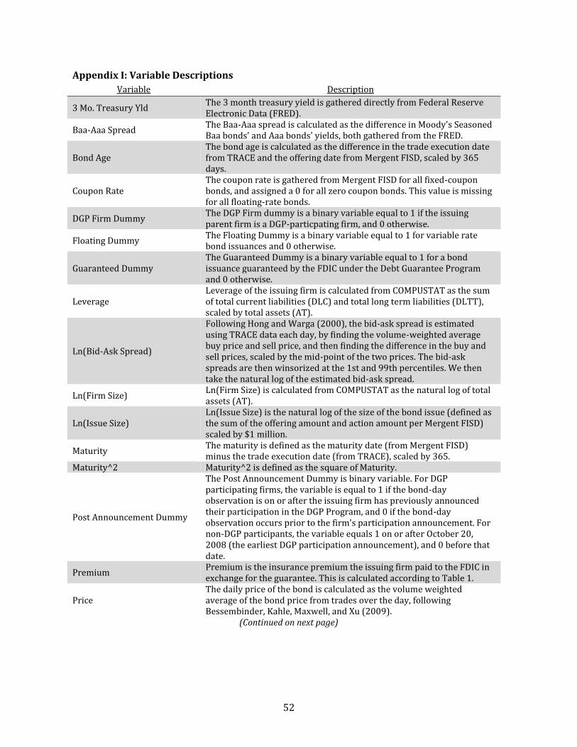
52

Appendix I: Variable Descriptions

Variable Description

3 Mo. Treasury Yld The 3 month treasury yield is gathered directly from Federal Reserve Electronic Data (FRED).

Baa-Aaa Spread The Baa-Aaa spread is calculated as the difference in Moody's Seasoned Baa bonds' and Aaa bonds' yields, both gathered from the FRED.

Bond Age The bond age is calculated as the difference in the trade execution date from TRACE and the offering date from Mergent FISD, scaled by 365 days.

Coupon Rate The coupon rate is gathered from Mergent FISD for all fixed-coupon bonds, and assigned a 0 for all zero coupon bonds. This value is missing for all floating-rate bonds.

DGP Firm Dummy The DGP Firm dummy is a binary variable equal to 1 if the issuing parent firm is a DGP-particpating firm, and 0 otherwise.

Floating Dummy The Floating Dummy is a binary variable equal to 1 for variable rate bond issuances and 0 otherwise.

Guaranteed Dummy The Guaranteed Dummy is a binary variable equal to 1 for a bond issuance guaranteed by the FDIC under the Debt Guarantee Program and 0 otherwise.

Leverage Leverage of the issuing firm is calculated from COMPUSTAT as the sum of total current liabilities (DLC) and total long term liabilities (DLTT), scaled by total assets (AT).

Ln(Bid-Ask Spread)

Following Hong and Warga (2000), the bid-ask spread is estimated using TRACE data each day, by finding the volume-weighted average buy price and sell price, and then finding the difference in the buy and sell prices, scaled by the mid-point of the two prices. The bid-ask spreads are then winsorized at the 1st and 99th percentiles. We then take the natural log of the estimated bid-ask spread.

Ln(Firm Size) Ln(Firm Size) is calculated from COMPUSTAT as the natural log of total assets (AT).

Ln(Issue Size) Ln(Issue Size) is the natural log of the size of the bond issue (defined as the sum of the offering amount and action amount per Mergent FISD) scaled by $1 million.

Maturity The maturity is defined as the maturity date (from Mergent FISD) minus the trade execution date (from TRACE), scaled by 365.

Maturity^2 Maturity^2 is defined as the square of Maturity.

Post Announcement Dummy

The Post Announcement Dummy is binary variable. For DGP participating firms, the variable is equal to 1 if the bond-day observation is on or after the issuing firm has previously announced their participation in the DGP Program, and 0 if the bond-day observation occurs prior to the firm's participation announcement. For non-DGP participants, the variable equals 1 on or after October 20, 2008 (the earliest DGP participation announcement), and 0 before that date.

Premium Premium is the insurance premium the issuing firm paid to the FDIC in exchange for the guarantee. This is calculated according to Table 1.

Price The daily price of the bond is calculated as the volume weighted average of the bond price from trades over the day, following Bessembinder, Kahle, Maxwell, and Xu (2009).

(Continued on next page)

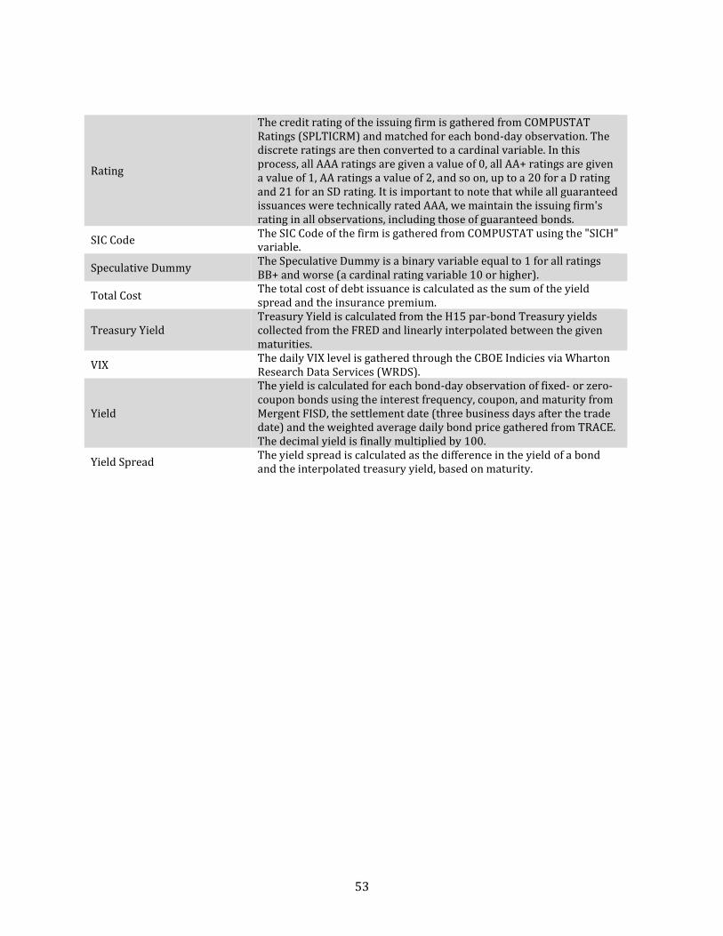
53

Rating

The credit rating of the issuing firm is gathered from COMPUSTAT Ratings (SPLTICRM) and matched for each bond-day observation. The discrete ratings are then converted to a cardinal variable. In this process, all AAA ratings are given a value of 0, all AA+ ratings are given a value of 1, AA ratings a value of 2, and so on, up to a 20 for a D rating and 21 for an SD rating. It is important to note that while all guaranteed issuances were technically rated AAA, we maintain the issuing firm's rating in all observations, including those of guaranteed bonds.

SIC Code The SIC Code of the firm is gathered from COMPUSTAT using the "SICH" variable.

Speculative Dummy The Speculative Dummy is a binary variable equal to 1 for all ratings BB+ and worse (a cardinal rating variable 10 or higher).

Total Cost The total cost of debt issuance is calculated as the sum of the yield spread and the insurance premium.

Treasury Yield Treasury Yield is calculated from the H15 par-bond Treasury yields collected from the FRED and linearly interpolated between the given maturities.

VIX The daily VIX level is gathered through the CBOE Indicies via Wharton Research Data Services (WRDS).

Yield

The yield is calculated for each bond-day observation of fixed- or zero-coupon bonds using the interest frequency, coupon, and maturity from Mergent FISD, the settlement date (three business days after the trade date) and the weighted average daily bond price gathered from TRACE. The decimal yield is finally multiplied by 100.

Yield Spread The yield spread is calculated as the difference in the yield of a bond and the interpolated treasury yield, based on maturity.

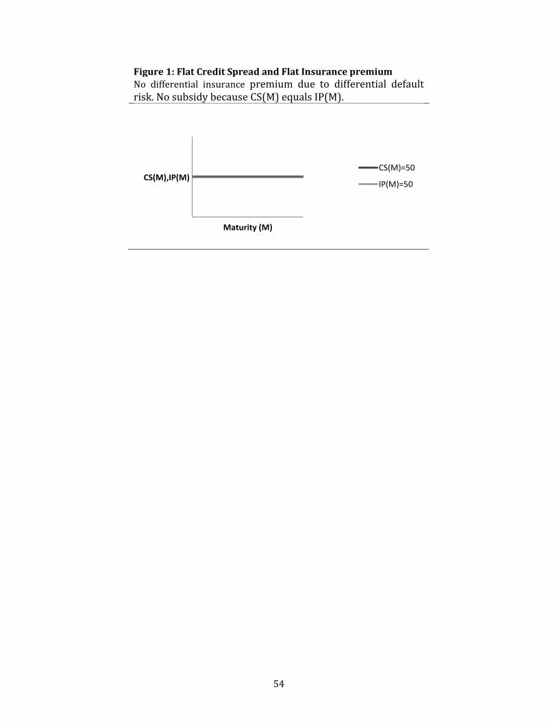
54

Figure 1: Flat Credit Spread and Flat Insurance premium No differential insurance premium due to differential default risk. No subsidy because CS(M) equals IP(M).

CS(M),IP(M)

Maturity (M)

CS(M)=50

IP(M)=50

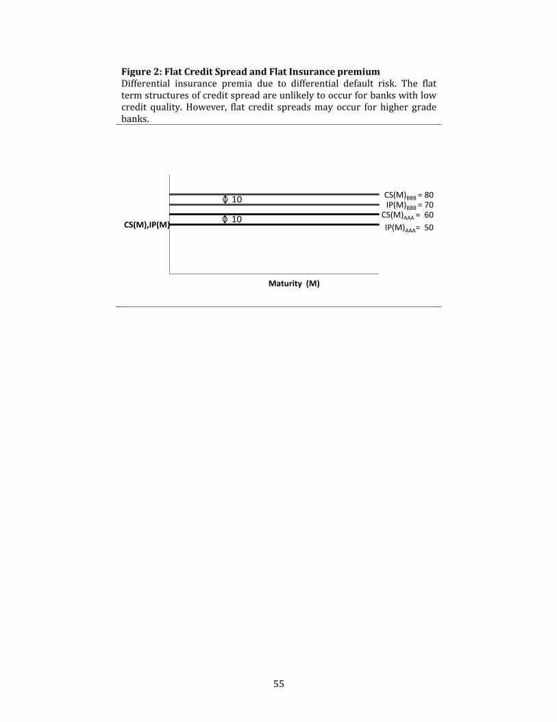
55

Figure 2: Flat Credit Spread and Flat Insurance premium Differential insurance premia due to differential default risk. The flat term structures of credit spread are unlikely to occur for banks with low credit quality. However, flat credit spreads may occur for higher grade banks.

CS(M)BBB = 80 IP(M)BBB = 70

CS(M)AAA = 60

IP(M)AAA= 50 CS(M),IP(M)

Maturity (M)

10

10

56

Figure 3: Flat Term Structures Equal IP(M) for both banks.

CS(M)BBB=80

CS(M)AAA=60

IP(M)AAA= IP(M)BBB

CS(M),IP(M)

Maturity (M)

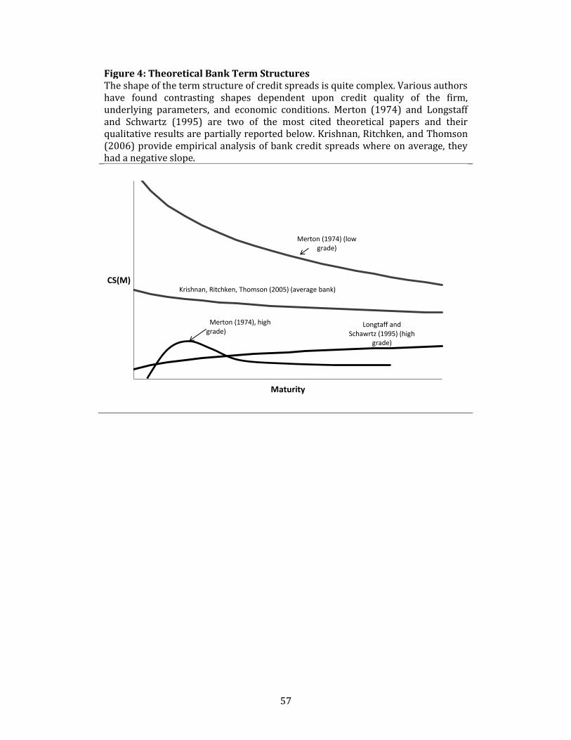
57

Figure 4: Theoretical Bank Term Structures The shape of the term structure of credit spreads is quite complex. Various authors have found contrasting shapes dependent upon credit quality of the firm, underlying parameters, and economic conditions. Merton (1974) and Longstaff and Schwartz (1995) are two of the most cited theoretical papers and their qualitative results are partially reported below. Krishnan, Ritchken, and Thomson (2006) provide empirical analysis of bank credit spreads where on average, they had a negative slope.

Merton (1974) (low grade)

Longtaff and Schawrtz (1995) (high

grade)

CS(M)

Maturity

Merton (1974), high grade)

Krishnan, Ritchken, Thomson (2005) (average bank)

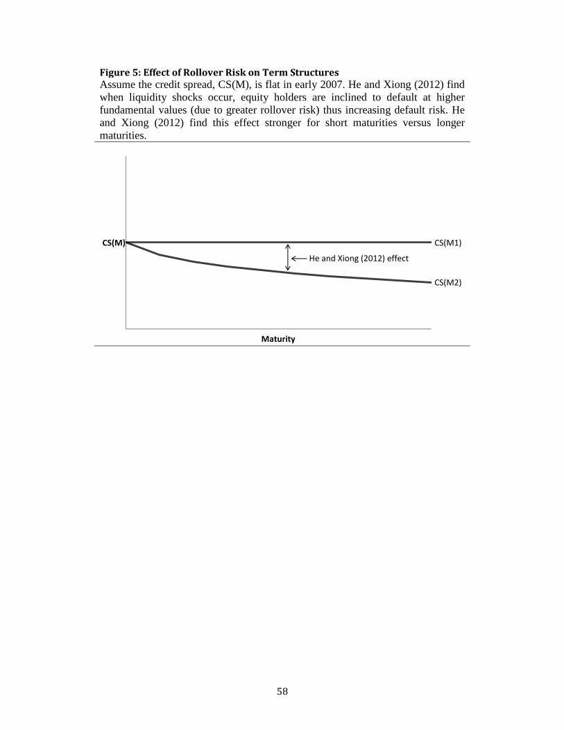
58

Figure 5: Effect of Rollover Risk on Term Structures Assume the credit spread, CS(M), is flat in early 2007. He and Xiong (2012) find

when liquidity shocks occur, equity holders are inclined to default at higher

fundamental values (due to greater rollover risk) thus increasing default risk. He

and Xiong (2012) find this effect stronger for short maturities versus longer

maturities.

CS(M2)

CS(M1) CS(M)

Maturity

He and Xiong (2012) effect

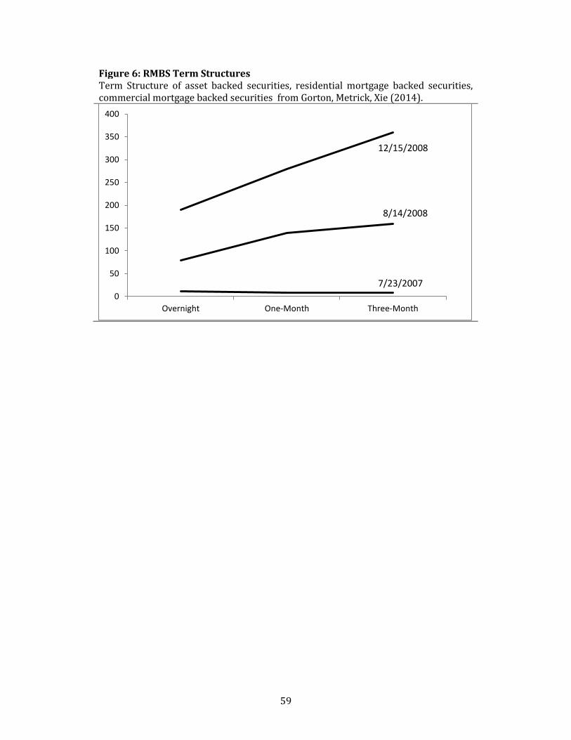
59

Figure 6: RMBS Term Structures Term Structure of asset backed securities, residential mortgage backed securities, commercial mortgage backed securities from Gorton, Metrick, Xie (2014).

0

50

100

150

200

250

300

350

400

Overnight One-Month Three-Month

7/23/2007

8/14/2008

12/15/2008

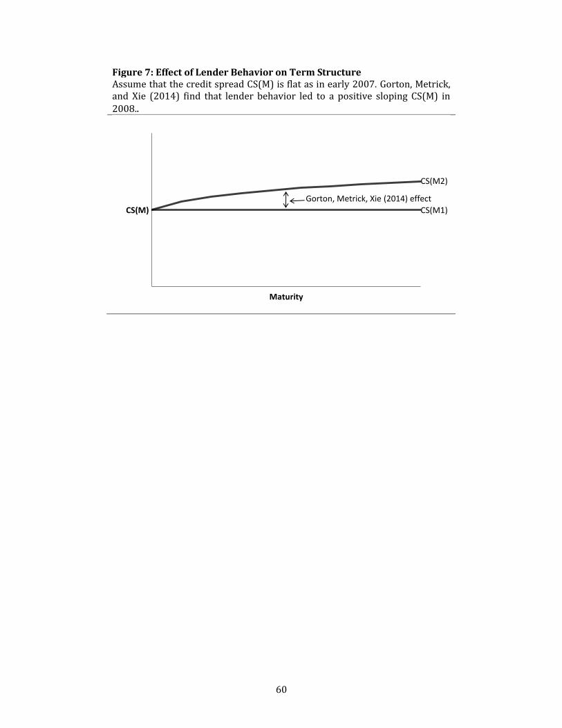
60

Figure 7: Effect of Lender Behavior on Term Structure Assume that the credit spread CS(M) is flat as in early 2007. Gorton, Metrick, and Xie (2014) find that lender behavior led to a positive sloping CS(M) in 2008..

CS(M2)

CS(M1) CS(M)

Maturity

Gorton, Metrick, Xie (2014) effect

61

Figure 8 Panel A 20 basis point benefit for negative CS term structure slopes.

Panel B 20 basis point benefit for flat CS TS slopes.

CS(M1)

IP(M1)

CS(M),IP(M)

Maturity (M)

20

CS(M2)

IP(M2)

CS(M),IP(M)

Maturity (M)

20

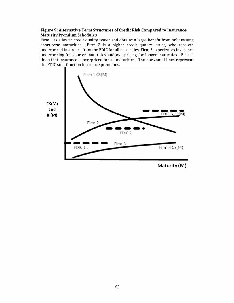
62

Figure 9: Alternative Term Structures of Credit Risk Compared to Insurance Maturity Premium Schedules Firm 1 is a lower credit quality issuer and obtains a large benefit from only issuing short-term maturities. Firm 2 is a higher credit quality issuer, who receives underpriced insurance from the FDIC for all maturities. Firm 3 experiences insurance underpricing for shorter maturities and overpricing for longer maturities. Firm 4 finds that insurance is overpriced for all maturities. The horizontal lines represent the FDIC step-function insurance premiums.

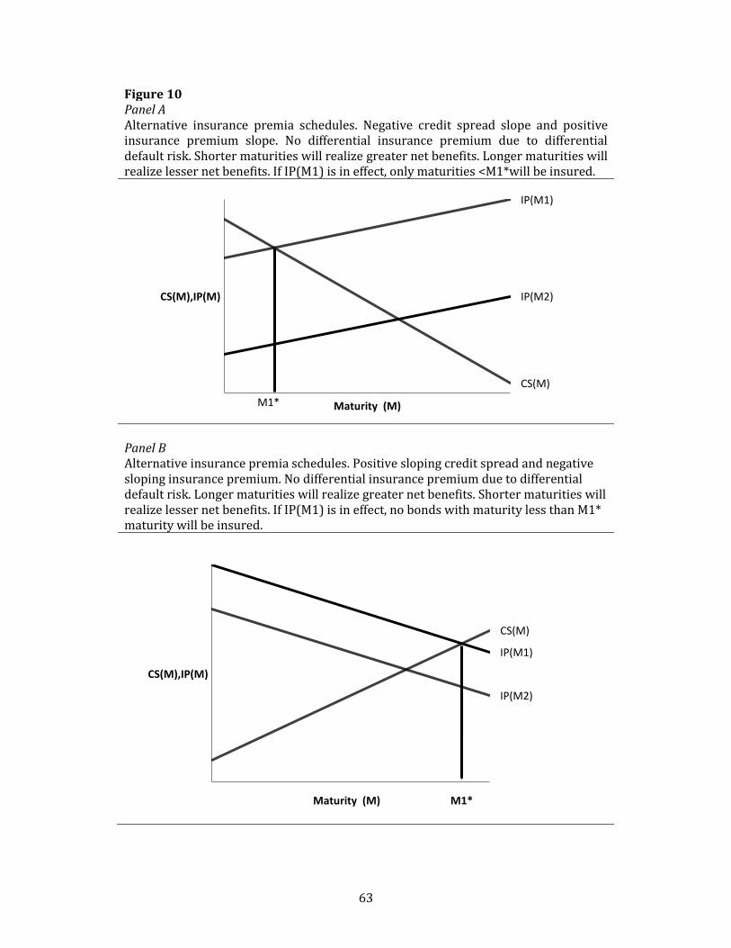
63

Figure 10 Panel A Alternative insurance premia schedules. Negative credit spread slope and positive insurance premium slope. No differential insurance premium due to differential default risk. Shorter maturities will realize greater net benefits. Longer maturities will realize lesser net benefits. If IP(M1) is in effect, only maturities <M1*will be insured.

Panel B Alternative insurance premia schedules. Positive sloping credit spread and negative sloping insurance premium. No differential insurance premium due to differential default risk. Longer maturities will realize greater net benefits. Shorter maturities will realize lesser net benefits. If IP(M1) is in effect, no bonds with maturity less than M1* maturity will be insured.

IP(M1)

CS(M)

IP(M2) CS(M),IP(M)

Maturity (M) M1*

IP(M2)

CS(M)

IP(M1)

CS(M),IP(M)

Maturity (M) M1*

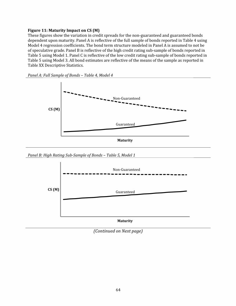
64

Figure 11: Maturity Impact on CS (M) These figures show the variation in credit spreads for the non-guaranteed and guaranteed bonds dependent upon maturity. Panel A is reflective of the full sample of bonds reported in Table 4 using Model 4 regression coefficients. The bond term structure modeled in Panel A is assumed to not be of speculative grade. Panel B is reflective of the high credit rating sub-sample of bonds reported in Table 5 using Model 1. Panel C is reflective of the low credit rating sub-sample of bonds reported in Table 5 using Model 3. All bond estimates are reflective of the means of the sample as reported in Table XX Descriptive Statistics. Panel A: Full Sample of Bonds – Table 4, Model 4

Panel B: High Rating Sub-Sample of Bonds – Table 5, Model 1

(Continued on Next page)

Non-Guaranteed

Guaranteed

CS (M)

Maturity

Non-Guaranteed

Guaranteed CS (M)

Maturity

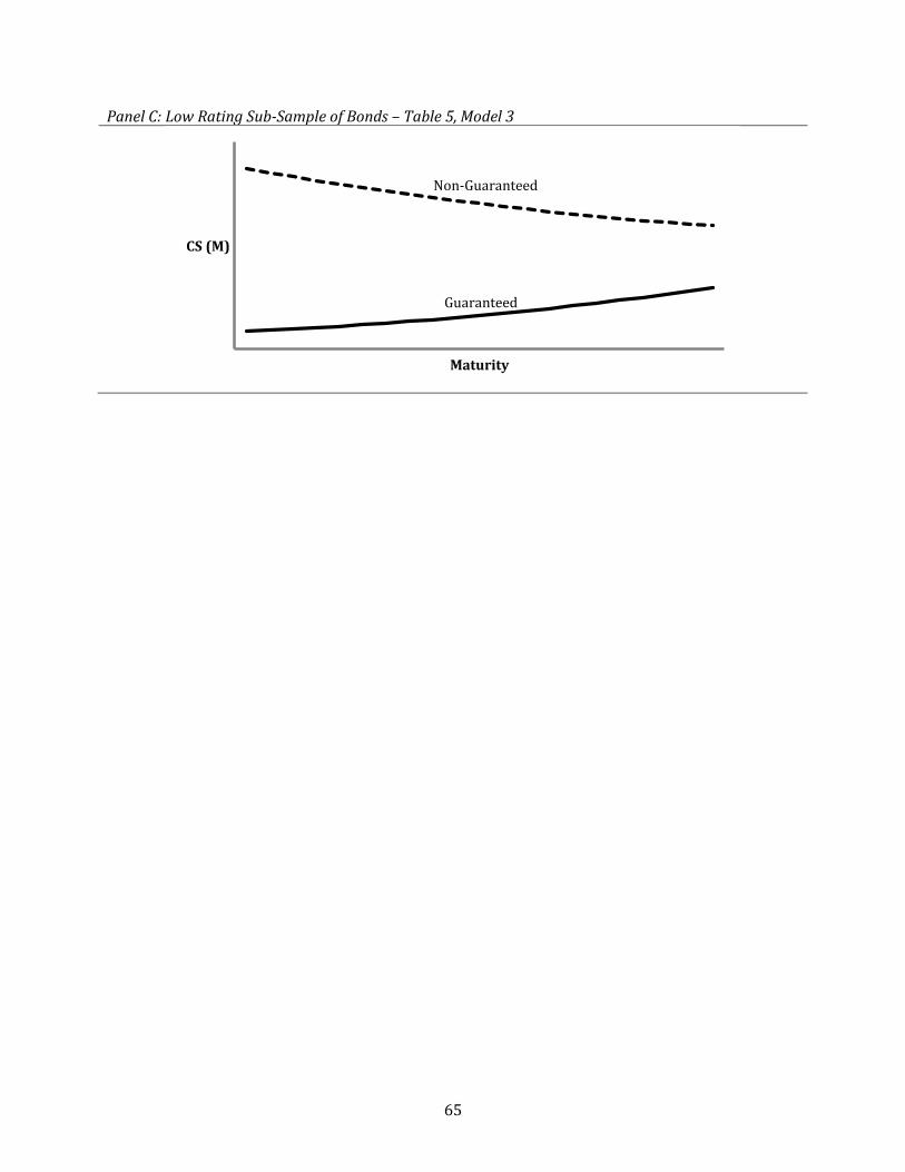
65

Panel C: Low Rating Sub-Sample of Bonds – Table 5, Model 3

Non-Guaranteed

Guaranteed

CS (M)

Maturity

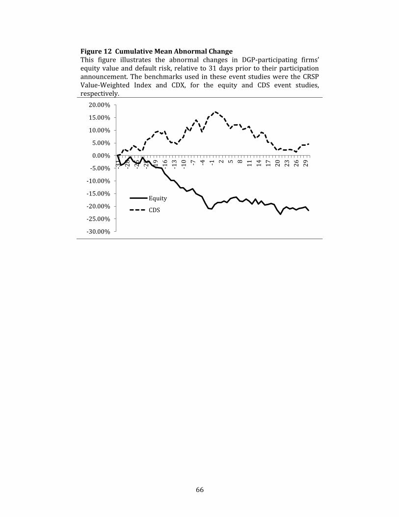
66

Figure 12 Cumulative Mean Abnormal Change This figure illustrates the abnormal changes in DGP-participating firms’ equity value and default risk, relative to 31 days prior to their participation announcement. The benchmarks used in these event studies were the CRSP Value-Weighted Index and CDX, for the equity and CDS event studies, respectively.

-30.00%

-25.00%

-20.00%

-15.00%

-10.00%

-5.00%

0.00%

5.00%

10.00%

15.00%

20.00%

-31

-28

-25

-22

-19

-16

-13

-10 -7 -4 -1 2 5 8

11

14

17

20

23

26

29

Equity

CDS

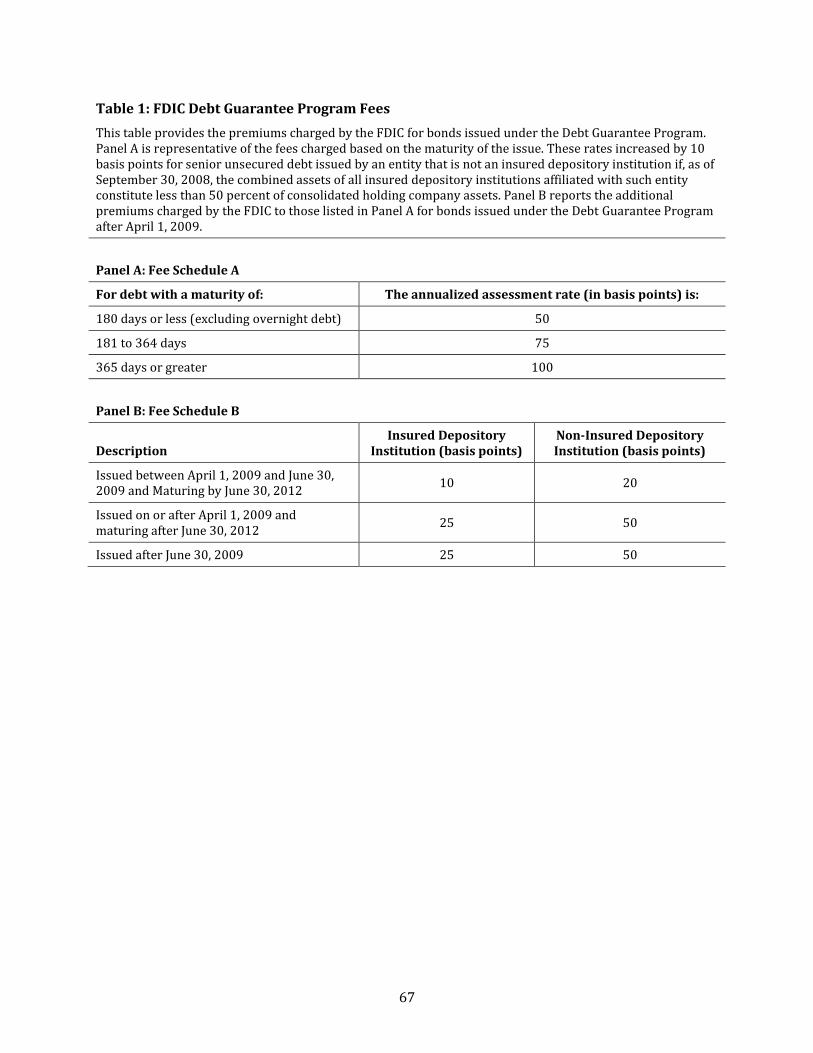
67

Table 1: FDIC Debt Guarantee Program Fees

This table provides the premiums charged by the FDIC for bonds issued under the Debt Guarantee Program. Panel A is representative of the fees charged based on the maturity of the issue. These rates increased by 10 basis points for senior unsecured debt issued by an entity that is not an insured depository institution if, as of September 30, 2008, the combined assets of all insured depository institutions affiliated with such entity constitute less than 50 percent of consolidated holding company assets. Panel B reports the additional premiums charged by the FDIC to those listed in Panel A for bonds issued under the Debt Guarantee Program after April 1, 2009.

Panel A: Fee Schedule A

For debt with a maturity of: The annualized assessment rate (in basis points) is:

180 days or less (excluding overnight debt) 50

181 to 364 days 75

365 days or greater 100

Panel B: Fee Schedule B

Description Insured Depository

Institution (basis points) Non-Insured Depository Institution (basis points)

Issued between April 1, 2009 and June 30, 2009 and Maturing by June 30, 2012

10 20

Issued on or after April 1, 2009 and maturing after June 30, 2012

25 50

Issued after June 30, 2009 25 50

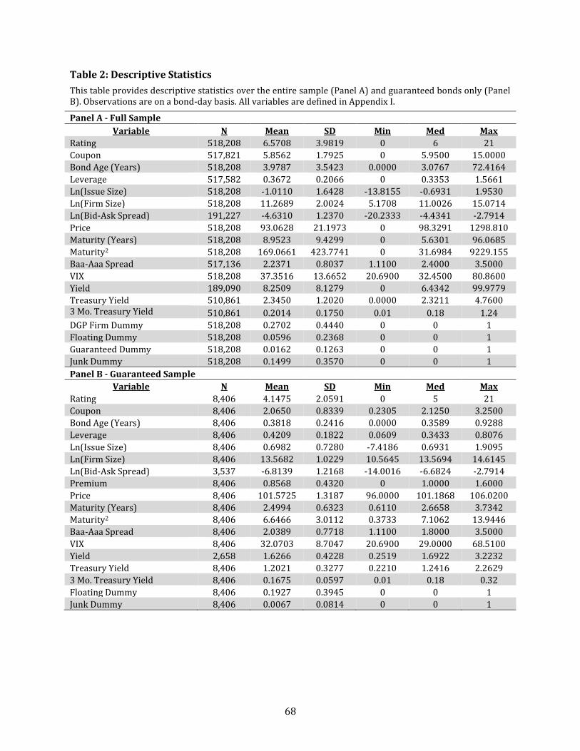
68

Table 2: Descriptive Statistics

This table provides descriptive statistics over the entire sample (Panel A) and guaranteed bonds only (Panel B). Observations are on a bond-day basis. All variables are defined in Appendix I.

Panel A - Full Sample

Variable N Mean SD Min Med Max

Rating 518,208 6.5708 3.9819 0 6 21

Coupon 517,821 5.8562 1.7925 0 5.9500 15.0000

Bond Age (Years) 518,208 3.9787 3.5423 0.0000 3.0767 72.4164

Leverage 517,582 0.3672 0.2066 0 0.3353 1.5661

Ln(Issue Size) 518,208 -1.0110 1.6428 -13.8155 -0.6931 1.9530

Ln(Firm Size) 518,208 11.2689 2.0024 5.1708 11.0026 15.0714

Ln(Bid-Ask Spread) 191,227 -4.6310 1.2370 -20.2333 -4.4341 -2.7914

Price 518,208 93.0628 21.1973 0 98.3291 1298.810

Maturity (Years) 518,208 8.9523 9.4299 0 5.6301 96.0685

Maturity2 518,208 169.0661 423.7741 0 31.6984 9229.155

Baa-Aaa Spread 517,136 2.2371 0.8037 1.1100 2.4000 3.5000

VIX 518,208 37.3516 13.6652 20.6900 32.4500 80.8600

Yield 189,090 8.2509 8.1279 0 6.4342 99.9779

Treasury Yield 510,861 2.3450 1.2020 0.0000 2.3211 4.7600 3 Mo. Treasury Yield 510,861 0.2014 0.1750 0.01 0.18 1.24

DGP Firm Dummy 518,208 0.2702 0.4440 0 0 1

Floating Dummy 518,208 0.0596 0.2368 0 0 1

Guaranteed Dummy 518,208 0.0162 0.1263 0 0 1

Junk Dummy 518,208 0.1499 0.3570 0 0 1

Panel B - Guaranteed Sample

Variable N Mean SD Min Med Max

Rating 8,406 4.1475 2.0591 0 5 21

Coupon 8,406 2.0650 0.8339 0.2305 2.1250 3.2500

Bond Age (Years) 8,406 0.3818 0.2416 0.0000 0.3589 0.9288

Leverage 8,406 0.4209 0.1822 0.0609 0.3433 0.8076

Ln(Issue Size) 8,406 0.6982 0.7280 -7.4186 0.6931 1.9095

Ln(Firm Size) 8,406 13.5682 1.0229 10.5645 13.5694 14.6145

Ln(Bid-Ask Spread) 3,537 -6.8139 1.2168 -14.0016 -6.6824 -2.7914

Premium 8,406 0.8568 0.4320 0 1.0000 1.6000

Price 8,406 101.5725 1.3187 96.0000 101.1868 106.0200

Maturity (Years) 8,406 2.4994 0.6323 0.6110 2.6658 3.7342

Maturity2 8,406 6.6466 3.0112 0.3733 7.1062 13.9446

Baa-Aaa Spread 8,406 2.0389 0.7718 1.1100 1.8000 3.5000

VIX 8,406 32.0703 8.7047 20.6900 29.0000 68.5100

Yield 2,658 1.6266 0.4228 0.2519 1.6922 3.2232

Treasury Yield 8,406 1.2021 0.3277 0.2210 1.2416 2.2629

3 Mo. Treasury Yield 8,406 0.1675 0.0597 0.01 0.18 0.32

Floating Dummy 8,406 0.1927 0.3945 0 0 1

Junk Dummy 8,406 0.0067 0.0814 0 0 1

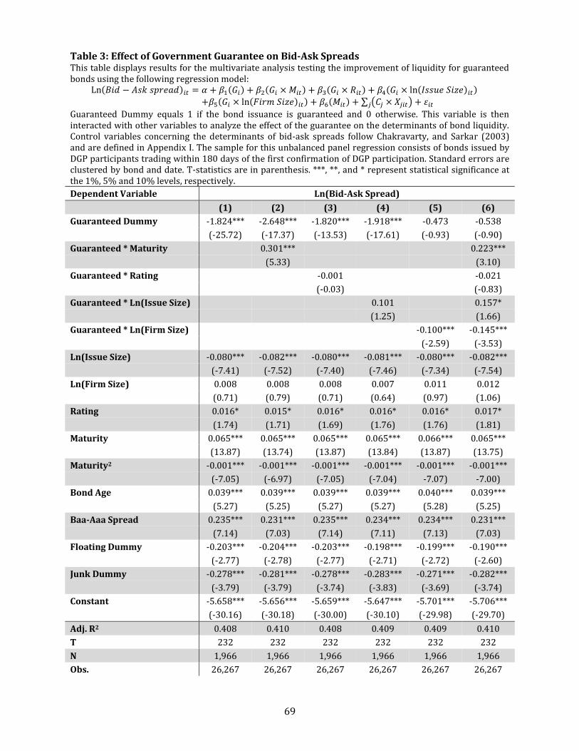
69

Table 3: Effect of Government Guarantee on Bid-Ask Spreads This table displays results for the multivariate analysis testing the improvement of liquidity for guaranteed bonds using the following regression model: Ln(𝐵𝑖𝑑 − 𝐴𝑠𝑘 𝑠𝑝𝑟𝑒𝑎𝑑)𝑖𝑡 = 𝛼 + 𝛽1(𝐺𝑖) + 𝛽2(𝐺𝑖 × 𝑀𝑖𝑡) + 𝛽3(𝐺𝑖 × 𝑅𝑖𝑡) + 𝛽4(𝐺𝑖 × ln(𝐼𝑠𝑠𝑢𝑒 𝑆𝑖𝑧𝑒)𝑖𝑡)

+𝛽5(𝐺𝑖 × ln(𝐹𝑖𝑟𝑚 𝑆𝑖𝑧𝑒)𝑖𝑡) + 𝛽6(𝑀𝑖𝑡) + ∑ (𝐶𝑗 × 𝑋𝑗𝑖𝑡)𝑗 + 𝜀𝑖𝑡

Guaranteed Dummy equals 1 if the bond issuance is guaranteed and 0 otherwise. This variable is then interacted with other variables to analyze the effect of the guarantee on the determinants of bond liquidity. Control variables concerning the determinants of bid-ask spreads follow Chakravarty, and Sarkar (2003) and are defined in Appendix I. The sample for this unbalanced panel regression consists of bonds issued by DGP participants trading within 180 days of the first confirmation of DGP participation. Standard errors are clustered by bond and date. T-statistics are in parenthesis. ***, **, and * represent statistical significance at the 1%, 5% and 10% levels, respectively.

Dependent Variable Ln(Bid-Ask Spread)

(1) (2) (3) (4) (5) (6)

Guaranteed Dummy -1.824*** -2.648*** -1.820*** -1.918*** -0.473 -0.538

(-25.72) (-17.37) (-13.53) (-17.61) (-0.93) (-0.90)

Guaranteed * Maturity

0.301***

0.223***

(5.33)

(3.10)

Guaranteed * Rating

-0.001

-0.021

(-0.03)

(-0.83)

Guaranteed * Ln(Issue Size)

0.101

0.157*

(1.25)

(1.66)

Guaranteed * Ln(Firm Size)

-0.100*** -0.145***

(-2.59) (-3.53)

Ln(Issue Size) -0.080*** -0.082*** -0.080*** -0.081*** -0.080*** -0.082***

(-7.41) (-7.52) (-7.40) (-7.46) (-7.34) (-7.54)

Ln(Firm Size) 0.008 0.008 0.008 0.007 0.011 0.012

(0.71) (0.79) (0.71) (0.64) (0.97) (1.06)

Rating 0.016* 0.015* 0.016* 0.016* 0.016* 0.017*

(1.74) (1.71) (1.69) (1.76) (1.76) (1.81)

Maturity 0.065*** 0.065*** 0.065*** 0.065*** 0.066*** 0.065***

(13.87) (13.74) (13.87) (13.84) (13.87) (13.75)

Maturity2 -0.001*** -0.001*** -0.001*** -0.001*** -0.001*** -0.001***

(-7.05) (-6.97) (-7.05) (-7.04) -7.07) -7.00)

Bond Age 0.039*** 0.039*** 0.039*** 0.039*** 0.040*** 0.039***

(5.27) (5.25) (5.27) (5.27) (5.28) (5.25)

Baa-Aaa Spread 0.235*** 0.231*** 0.235*** 0.234*** 0.234*** 0.231***

(7.14) (7.03) (7.14) (7.11) (7.13) (7.03)

Floating Dummy -0.203*** -0.204*** -0.203*** -0.198*** -0.199*** -0.190***

(-2.77) (-2.78) (-2.77) (-2.71) (-2.72) (-2.60)

Junk Dummy -0.278*** -0.281*** -0.278*** -0.283*** -0.271*** -0.282***

(-3.79) (-3.79) (-3.74) (-3.83) (-3.69) (-3.74)

Constant -5.658*** -5.656*** -5.659*** -5.647*** -5.701*** -5.706***

(-30.16) (-30.18) (-30.00) (-30.10) (-29.98) (-29.70)

Adj. R2 0.408 0.410 0.408 0.409 0.409 0.410

T 232 232 232 232 232 232

N 1,966 1,966 1,966 1,966 1,966 1,966

Obs. 26,267 26,267 26,267 26,267 26,267 26,267

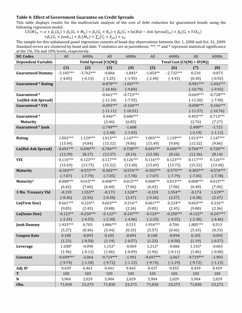
Table 4: Effect of Government Guarantee on Credit Spreads This table displays results for the multivariate analysis of the cost of debt reduction for guaranteed bonds using the following regression model: 𝐶𝑆(𝑀)𝑖𝑡 = 𝛼 + 𝛽1(𝐺𝑖) + 𝛽2(𝐺𝑖 × 𝑀𝑖𝑡) + 𝛽3(𝐺𝑖 × 𝑅𝑖𝑡) + 𝛽4(𝐺𝑖 × ln(𝐵𝑖𝑑 − 𝐴𝑠𝑘 𝑆𝑝𝑟𝑒𝑎𝑑)𝑖𝑡) + 𝛽5(𝐺𝑖 × 𝑉𝐼𝑋𝑖𝑡)

+𝛽5(𝐺𝑖 × 𝐽𝑢𝑛𝑘𝑖𝑡) + 𝛽7(𝑀𝑖𝑡) + ∑ (𝐶𝑗 × 𝑋𝑗𝑖𝑡)𝑗 + 𝜀𝑖𝑡

The sample for this unbalanced panel regression consists of bond-day observations between Oct. 1, 2008 and Oct. 31, 2009. Standard errors are clustered by bond and date. T-statistics are in parenthesis. ***, ** and * represent statistical significance at the 1%, 5% and 10% levels, respectively.

SIC Codes All 6000s All 6000s All 6000s All 6000s

Dependent Variable Yield Spread [CS(M)] Total Cost [CS(M) + IP(M)]

(1) (2) (3) (4) (5) (6) (7) (8)

Guaranteed Dummy -2.105*** -3.762*** -0.866 -1.845* -1.054** -2.732*** 0.210 -0.873

(-4.83) (-6.13) (-1.25) (-1.95) (-2.40) (-4.45) (0.30) (-0.92)

Guaranteed * Rating

-0.878*** -1.047***

-0.901*** -1.042***

(-10.40) (-9.84)

(-10.79) (-9.93)

Guaranteed *

-0.661*** -0.723***

-0.669*** -0.728***

Ln(Bid-Ask Spread)

(-11.34) (-7.93)

(-11.50) (-7.98)

Guaranteed * VIX

-0.095*** -0.104***

-0.098*** -0.106***

(-11.11) (-10.51)

(-11.57) (-10.76)

Guaranteed *

0.446** 0.686***

0.492*** 0.713***

Maturity

(2.46) (6.85)

(2.76) (7.27)

Guaranteed * Junk

-2.749*** -1.608

-2.400** -1.721

(-2.48) (-1.03)

(-2.19) (-1.12)

Rating 1.003*** 1.129*** 1.013*** 1.147*** 1.003*** 1.129*** 1.013*** 1.147***

(15.49) (9.84) (15.52) (9.86) (15.49) (9.84) (15.52) (9.86)

Ln(Bid-Ask Spread) 0.691*** 0.690*** 0.704*** 0.728*** 0.691*** 0.690*** 0.704*** 0.728***

(12.39) (8.17) (12.37) (8.14) (12.38) (8.16) (12.36) (8.14)

VIX 0.116*** 0.123*** 0.117*** 0.126*** 0.116*** 0.123*** 0.117*** 0.126***

(15.69) (13.75) (15.52) (13.48) (15.69) (13.75) (15.52) (13.48)

Maturity -0.303*** -0.575*** -0.303*** -0.576*** -0.303*** -0.575*** -0.303*** -0.576***

(-7.07) (-7.79) (-7.05) (-7.78) (-7.07) (-7.79) (-7.05) (-7.78)

Maturity2 0.008*** 0.015*** 0.008*** 0.015*** 0.008*** 0.015*** 0.008*** 0.015***

(6.42) (7.06) (6.40) (7.06) (6.42) (7.06) (6.40) (7.06)

3 Mo. Treasury Yld -0.159 1.553** -0.173 1.520** -0.159 1.554** -0.174 1.519**

(-0.36) (2.56) (-0.38) (2.47) (-0.36) (2.57) (-0.38) (2.47)

Ln(Firm Size) 0.661*** 0.224** 0.663*** 0.216** 0.661*** 0.224** 0.663*** 0.216**

(9.85) (2.45) (9.88) (2.36) (9.85) (2.45) (9.88) (2.36)

Ln(Issue Size) -0.123** -0.250*** -0.122** -0.247*** -0.124** -0.250*** -0.122** -0.247***

(-2.33) (-4.55) (-2.30) (-4.46) (-2.33) (-4.55) (-2.30) (-4.46)

Junk Dummy 1.933*** 0.703 1.886*** 0.515 1.934*** 0.700 1.885*** 0.513

(5.57) (0.46) (5.44) (0.33) (5.57) (0.46) (5.43) (0.33)

Coupon Rate 0.108 -0.093 0.105 -0.091 0.108 -0.094 0.105 -0.092

(1.23) (-0.58) (1.19) (-0.57) (1.23) (-0.58) (1.19) (-0.57)

Leverage 1.208* -0.090 1.152* -0.069 1.212* -0.086 1.155* -0.065

(1.96) (-0.12) (1.86) (-0.09) (1.96) (-0.11) (1.86) (-0.08)

Constant -9.699*** -2.064 -9.719*** -1.991 -9.697*** -2.067 -9.719*** -1.993

(-9.74) (-1.18) (-9.72) (-1.13) (-9.74) (-1.19) (-9.72) (-1.13)

Adj. R2 0.439 0.461 0.441 0.465 0.437 0.455 0.439 0.459

T 105 105 105 105 105 105 105 105

N 5,904 2,029 5,904 2,029 5,904 2,029 5,904 2,029

Obs. 71,830 23,273 71,830 23,273 71,830 23,273 71,830 23,273

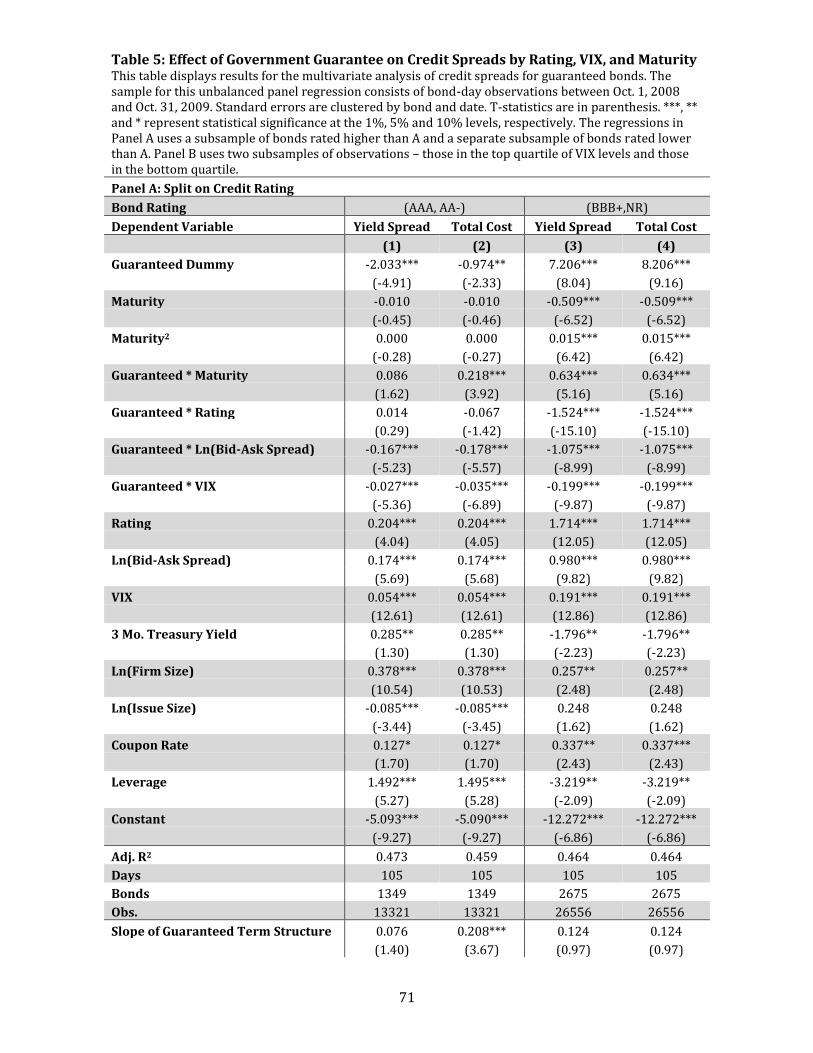
71

Table 5: Effect of Government Guarantee on Credit Spreads by Rating, VIX, and Maturity This table displays results for the multivariate analysis of credit spreads for guaranteed bonds. The sample for this unbalanced panel regression consists of bond-day observations between Oct. 1, 2008 and Oct. 31, 2009. Standard errors are clustered by bond and date. T-statistics are in parenthesis. ***, ** and * represent statistical significance at the 1%, 5% and 10% levels, respectively. The regressions in Panel A uses a subsample of bonds rated higher than A and a separate subsample of bonds rated lower than A. Panel B uses two subsamples of observations – those in the top quartile of VIX levels and those in the bottom quartile.

Panel A: Split on Credit Rating

Bond Rating (AAA, AA-) (BBB+,NR)

Dependent Variable Yield Spread Total Cost Yield Spread Total Cost

(1) (2) (3) (4)

Guaranteed Dummy -2.033*** -0.974** 7.206*** 8.206***

(-4.91) (-2.33) (8.04) (9.16)

Maturity -0.010 -0.010 -0.509*** -0.509***

(-0.45) (-0.46) (-6.52) (-6.52)

Maturity2 0.000 0.000 0.015*** 0.015***

(-0.28) (-0.27) (6.42) (6.42)

Guaranteed * Maturity 0.086 0.218*** 0.634*** 0.634***

(1.62) (3.92) (5.16) (5.16)

Guaranteed * Rating 0.014 -0.067 -1.524*** -1.524***

(0.29) (-1.42) (-15.10) (-15.10)

Guaranteed * Ln(Bid-Ask Spread) -0.167*** -0.178*** -1.075*** -1.075***

(-5.23) (-5.57) (-8.99) (-8.99)

Guaranteed * VIX -0.027*** -0.035*** -0.199*** -0.199***

(-5.36) (-6.89) (-9.87) (-9.87)

Rating 0.204*** 0.204*** 1.714*** 1.714***

(4.04) (4.05) (12.05) (12.05)

Ln(Bid-Ask Spread) 0.174*** 0.174*** 0.980*** 0.980***

(5.69) (5.68) (9.82) (9.82)

VIX 0.054*** 0.054*** 0.191*** 0.191***

(12.61) (12.61) (12.86) (12.86)

3 Mo. Treasury Yield 0.285** 0.285** -1.796** -1.796**

(1.30) (1.30) (-2.23) (-2.23)

Ln(Firm Size) 0.378*** 0.378*** 0.257** 0.257**

(10.54) (10.53) (2.48) (2.48)

Ln(Issue Size) -0.085*** -0.085*** 0.248 0.248

(-3.44) (-3.45) (1.62) (1.62)

Coupon Rate 0.127* 0.127* 0.337** 0.337***

(1.70) (1.70) (2.43) (2.43)

Leverage 1.492*** 1.495*** -3.219** -3.219**

(5.27) (5.28) (-2.09) (-2.09)

Constant -5.093*** -5.090*** -12.272*** -12.272***

(-9.27) (-9.27) (-6.86) (-6.86)

Adj. R2 0.473 0.459 0.464 0.464

Days 105 105 105 105

Bonds 1349 1349 2675 2675

Obs. 13321 13321 26556 26556

Slope of Guaranteed Term Structure 0.076 0.208*** 0.124 0.124

(1.40) (3.67) (0.97) (0.97)

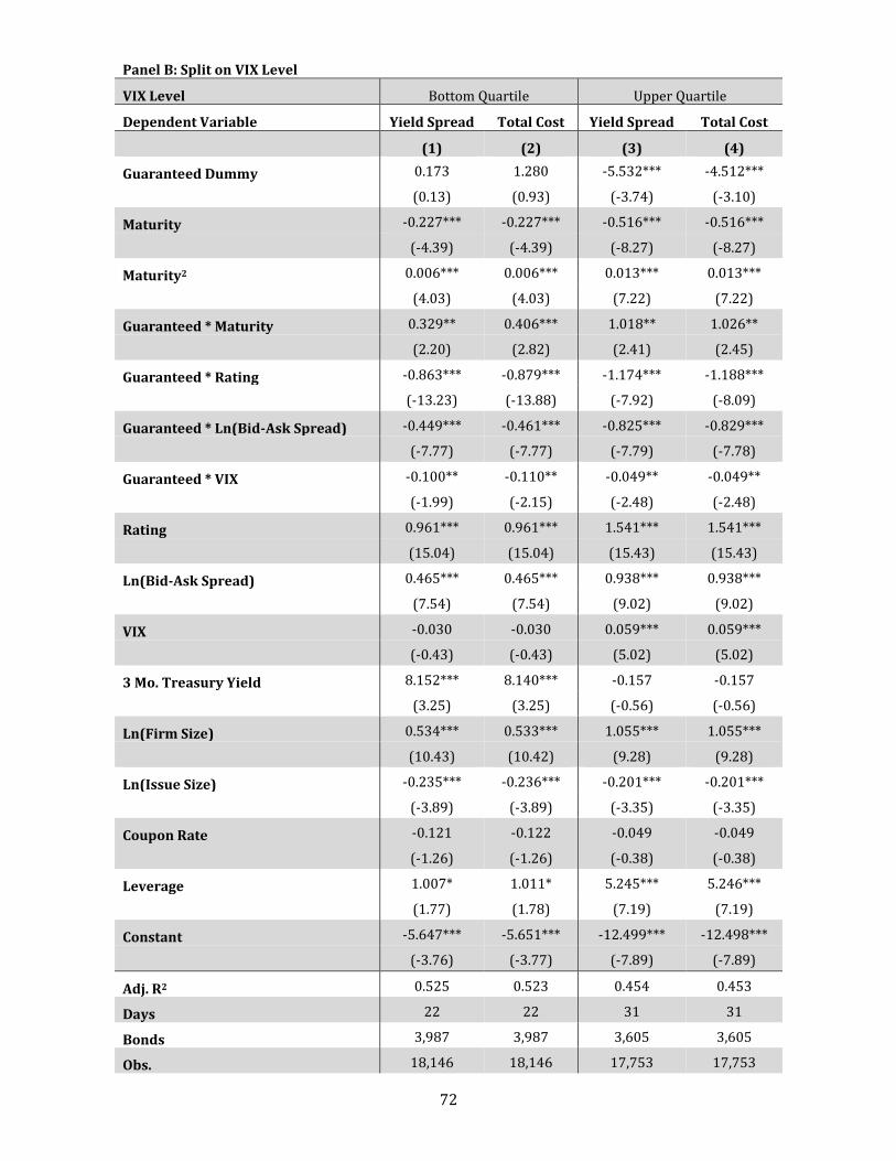
72

Panel B: Split on VIX Level

VIX Level Bottom Quartile Upper Quartile

Dependent Variable Yield Spread Total Cost Yield Spread Total Cost

(1) (2) (3) (4)

Guaranteed Dummy 0.173 1.280 -5.532*** -4.512***

(0.13) (0.93) (-3.74) (-3.10)

Maturity -0.227*** -0.227*** -0.516*** -0.516***

(-4.39) (-4.39) (-8.27) (-8.27)

Maturity2 0.006*** 0.006*** 0.013*** 0.013***

(4.03) (4.03) (7.22) (7.22)

Guaranteed * Maturity 0.329** 0.406*** 1.018** 1.026**

(2.20) (2.82) (2.41) (2.45)

Guaranteed * Rating -0.863*** -0.879*** -1.174*** -1.188***

(-13.23) (-13.88) (-7.92) (-8.09)

Guaranteed * Ln(Bid-Ask Spread) -0.449*** -0.461*** -0.825*** -0.829***

(-7.77) (-7.77) (-7.79) (-7.78)

Guaranteed * VIX -0.100** -0.110** -0.049** -0.049**

(-1.99) (-2.15) (-2.48) (-2.48)

Rating 0.961*** 0.961*** 1.541*** 1.541***

(15.04) (15.04) (15.43) (15.43)

Ln(Bid-Ask Spread) 0.465*** 0.465*** 0.938*** 0.938***

(7.54) (7.54) (9.02) (9.02)

VIX -0.030 -0.030 0.059*** 0.059***

(-0.43) (-0.43) (5.02) (5.02)

3 Mo. Treasury Yield 8.152*** 8.140*** -0.157 -0.157

(3.25) (3.25) (-0.56) (-0.56)

Ln(Firm Size) 0.534*** 0.533*** 1.055*** 1.055***

(10.43) (10.42) (9.28) (9.28)

Ln(Issue Size) -0.235*** -0.236*** -0.201*** -0.201***

(-3.89) (-3.89) (-3.35) (-3.35)

Coupon Rate -0.121 -0.122 -0.049 -0.049

(-1.26) (-1.26) (-0.38) (-0.38)

Leverage 1.007* 1.011* 5.245*** 5.246***

(1.77) (1.78) (7.19) (7.19)

Constant -5.647*** -5.651*** -12.499*** -12.498***

(-3.76) (-3.77) (-7.89) (-7.89)

Adj. R2 0.525 0.523 0.454 0.453

Days 22 22 31 31

Bonds 3,987 3,987 3,605 3,605

Obs. 18,146 18,146 17,753 17,753

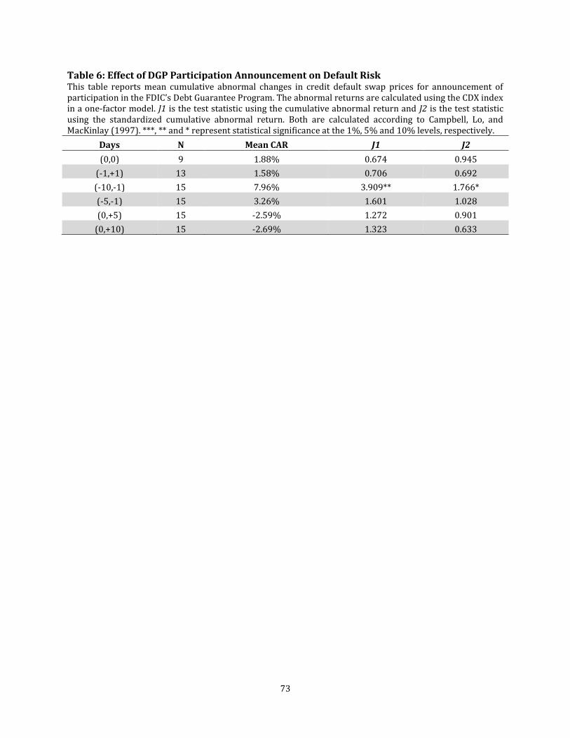
73

Table 6: Effect of DGP Participation Announcement on Default Risk This table reports mean cumulative abnormal changes in credit default swap prices for announcement of participation in the FDIC’s Debt Guarantee Program. The abnormal returns are calculated using the CDX index in a one-factor model. J1 is the test statistic using the cumulative abnormal return and J2 is the test statistic using the standardized cumulative abnormal return. Both are calculated according to Campbell, Lo, and MacKinlay (1997). ***, ** and * represent statistical significance at the 1%, 5% and 10% levels, respectively.

Days N Mean CAR J1 J2

(0,0) 9 1.88% 0.674 0.945

(-1,+1) 13 1.58% 0.706 0.692

(-10,-1) 15 7.96% 3.909** 1.766*

(-5,-1) 15 3.26% 1.601 1.028

(0,+5) 15 -2.59% 1.272 0.901

(0,+10) 15 -2.69% 1.323 0.633

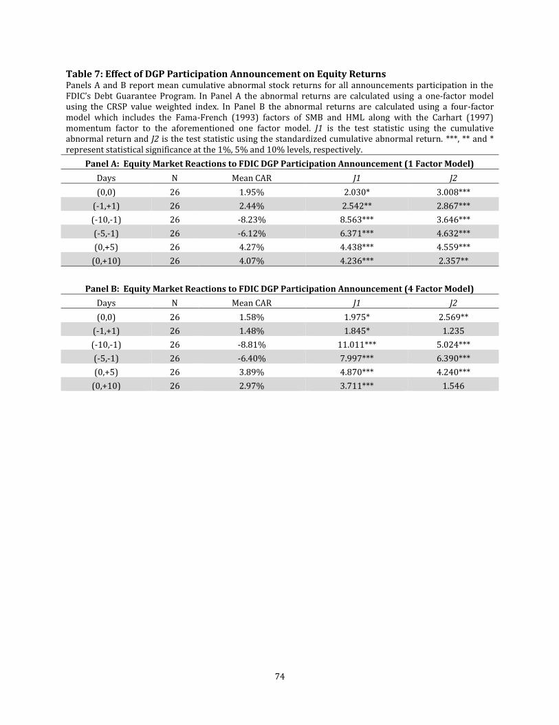
74

Table 7: Effect of DGP Participation Announcement on Equity Returns Panels A and B report mean cumulative abnormal stock returns for all announcements participation in the FDIC’s Debt Guarantee Program. In Panel A the abnormal returns are calculated using a one-factor model using the CRSP value weighted index. In Panel B the abnormal returns are calculated using a four-factor model which includes the Fama-French (1993) factors of SMB and HML along with the Carhart (1997) momentum factor to the aforementioned one factor model. J1 is the test statistic using the cumulative abnormal return and J2 is the test statistic using the standardized cumulative abnormal return. ***, ** and * represent statistical significance at the 1%, 5% and 10% levels, respectively.

Panel A: Equity Market Reactions to FDIC DGP Participation Announcement (1 Factor Model)

Days N Mean CAR J1 J2

(0,0) 26 1.95% 2.030* 3.008***

(-1,+1) 26 2.44% 2.542** 2.867***

(-10,-1) 26 -8.23% 8.563*** 3.646***

(-5,-1) 26 -6.12% 6.371*** 4.632***

(0,+5) 26 4.27% 4.438*** 4.559***

(0,+10) 26 4.07% 4.236*** 2.357**

Panel B: Equity Market Reactions to FDIC DGP Participation Announcement (4 Factor Model)

Days N Mean CAR J1 J2

(0,0) 26 1.58% 1.975* 2.569**

(-1,+1) 26 1.48% 1.845* 1.235

(-10,-1) 26 -8.81% 11.011*** 5.024***

(-5,-1) 26 -6.40% 7.997*** 6.390***

(0,+5) 26 3.89% 4.870*** 4.240***

(0,+10) 26 2.97% 3.711*** 1.546

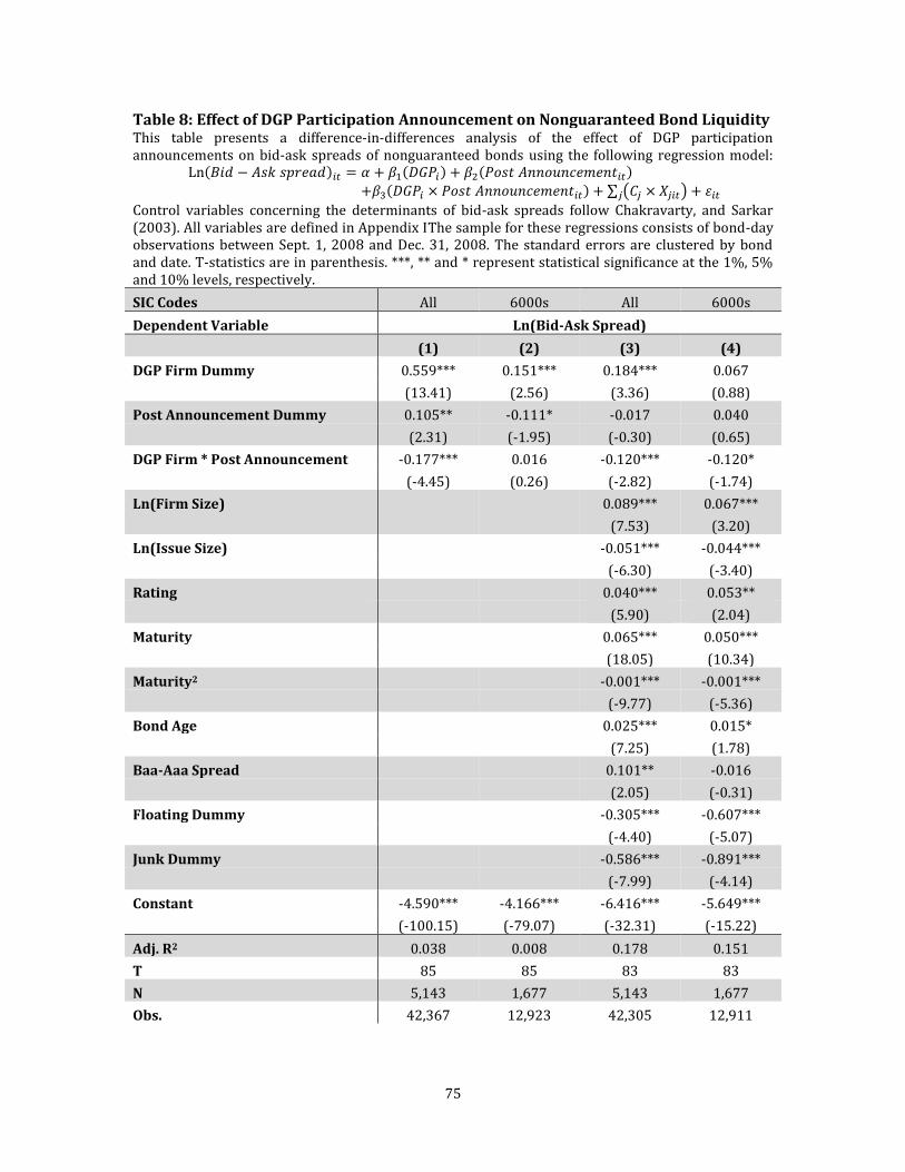
75

Table 8: Effect of DGP Participation Announcement on Nonguaranteed Bond Liquidity This table presents a difference-in-differences analysis of the effect of DGP participation announcements on bid-ask spreads of nonguaranteed bonds using the following regression model: Ln(𝐵𝑖𝑑 − 𝐴𝑠𝑘 𝑠𝑝𝑟𝑒𝑎𝑑)𝑖𝑡 = 𝛼 + 𝛽1(𝐷𝐺𝑃𝑖) + 𝛽2(𝑃𝑜𝑠𝑡 𝐴𝑛𝑛𝑜𝑢𝑛𝑐𝑒𝑚𝑒𝑛𝑡𝑖𝑡)

+𝛽3(𝐷𝐺𝑃𝑖 × 𝑃𝑜𝑠𝑡 𝐴𝑛𝑛𝑜𝑢𝑛𝑐𝑒𝑚𝑒𝑛𝑡𝑖𝑡) + ∑ (𝐶𝑗 × 𝑋𝑗𝑖𝑡)𝑗 + 𝜀𝑖𝑡

Control variables concerning the determinants of bid-ask spreads follow Chakravarty, and Sarkar (2003). All variables are defined in Appendix IThe sample for these regressions consists of bond-day observations between Sept. 1, 2008 and Dec. 31, 2008. The standard errors are clustered by bond and date. T-statistics are in parenthesis. ***, ** and * represent statistical significance at the 1%, 5% and 10% levels, respectively.

SIC Codes All 6000s All 6000s

Dependent Variable Ln(Bid-Ask Spread)

(1) (2) (3) (4)

DGP Firm Dummy 0.559*** 0.151*** 0.184*** 0.067

(13.41) (2.56) (3.36) (0.88)

Post Announcement Dummy 0.105** -0.111* -0.017 0.040

(2.31) (-1.95) (-0.30) (0.65)

DGP Firm * Post Announcement -0.177*** 0.016 -0.120*** -0.120*

(-4.45) (0.26) (-2.82) (-1.74)

Ln(Firm Size)

0.089*** 0.067***

(7.53) (3.20)

Ln(Issue Size)

-0.051*** -0.044***

(-6.30) (-3.40)

Rating

0.040*** 0.053**

(5.90) (2.04)

Maturity

0.065*** 0.050***

(18.05) (10.34)

Maturity2

-0.001*** -0.001***

(-9.77) (-5.36)

Bond Age

0.025*** 0.015*

(7.25) (1.78)

Baa-Aaa Spread

0.101** -0.016

(2.05) (-0.31)

Floating Dummy

-0.305*** -0.607***

(-4.40) (-5.07)

Junk Dummy

-0.586*** -0.891***

(-7.99) (-4.14)

Constant -4.590*** -4.166*** -6.416*** -5.649***

(-100.15) (-79.07) (-32.31) (-15.22)

Adj. R2 0.038 0.008 0.178 0.151

T 85 85 83 83

N 5,143 1,677 5,143 1,677

Obs. 42,367 12,923 42,305 12,911