arX

iv:1

707.

0909

2v3

[cs

.CV

] 4

Apr

201

8

This is an extended version of a paper accepted for publication at CVPR 2018. Main part of the paper: c©2018 IEEE

Benchmarking 6DOF Outdoor Visual Localization in Changing Conditions

Torsten Sattler1 Will Maddern2 Carl Toft3 Akihiko Torii4 Lars Hammarstrand3

Erik Stenborg3 Daniel Safari4,5 Masatoshi Okutomi4 Marc Pollefeys1,6

Josef Sivic7,8 Fredrik Kahl3,9 Tomas Pajdla8

1Department of Computer Science, ETH Zurich 2Oxford Robotics Institute, University of Oxford3Department of Electrical Engineering, Chalmers University of Technology 6Microsoft

4Tokyo Institute of Technology 5Technical University of Denmark 7Inria∗

8CIIRC, CTU in Prague† 9Centre for Mathematical Sciences, Lund University

Abstract

Visual localization enables autonomous vehicles to navi-

gate in their surroundings and augmented reality applica-

tions to link virtual to real worlds. Practical visual local-

ization approaches need to be robust to a wide variety of

viewing condition, including day-night changes, as well as

weather and seasonal variations, while providing highly ac-

curate 6 degree-of-freedom (6DOF) camera pose estimates.

In this paper, we introduce the first benchmark datasets

specifically designed for analyzing the impact of such fac-

tors on visual localization. Using carefully created ground

truth poses for query images taken under a wide variety

of conditions, we evaluate the impact of various factors on

6DOF camera pose estimation accuracy through extensive

experiments with state-of-the-art localization approaches.

Based on our results, we draw conclusions about the diffi-

culty of different conditions, showing that long-term local-

ization is far from solved, and propose promising avenues

for future work, including sequence-based localization ap-

proaches and the need for better local features. Our bench-

mark is available at visuallocalization.net.

1. Introduction

Estimating the 6DOF camera pose of an image with re-

spect to a 3D scene model is key for visual navigation of

autonomous vehicles and augmented/mixed reality devices.

Solutions to this visual localization problem can also be

used to “close loops” in the context of SLAM or to register

images to Structure-from-Motion (SfM) reconstructions.

Work on 3D structure-based visual localization has fo-

cused on increasing efficiency [34, 37, 44, 58, 71], improv-

ing scalability and robustness to ambiguous structures [36,

∗WILLOW project, Departement d’Informatique de l’Ecole Normale

Superieure, ENS/INRIA/CNRS UMR 8548, PSL Research University.†CIIRC - Czech Institute of Informatics, Robotics, and Cybernetics,

Czech Technical University in Prague

Figure 1. Visual localization in changing urban conditions. We

present three new datasets, Aachen Day-Night, RobotCar Sea-

sons (shown) and CMU Seasons for evaluating 6DOF localization

against a prior 3D map (top) using registered query images taken

from a wide variety of conditions (bottom), including day-night

variation, weather, and seasonal changes over long periods of time.

56,70,81], reducing memory requirements [13,37,56], and

more flexible scene representations [59]. All these methods

utilize local features to establish 2D-3D matches. These

correspondences are in turn used to estimate the camera

pose. This data association stage is critical as pose estima-

tion fails without sufficiently many correct matches. There

is a well-known trade-off between discriminative power and

invariance for local descriptors. Thus, existing localization

approaches will only find enough matches if both the query

images and the images used to construct the 3D scene model

are taken under similar viewing conditions.

Capturing a scene under all viewing conditions is pro-

hibitive. Thus, the assumption that all relevant conditions

are covered is too restrictive in practice. It is more realis-

tic to expect that images of a scene are taken under a sin-

gle or a few conditions. To be practically relevant, e.g., for

1

life-long localization for self-driving cars, visual localiza-

tion algorithms need to be robust under varying conditions

(cf . Fig. 1). Yet, no work in the literature actually measures

the impact of varying conditions on 6DOF pose accuracy.

One reason for the lack of work on visual localization

under varying conditions is a lack of suitable benchmark

datasets. The standard approach for obtaining ground truth

6DOF poses for query images is to use SfM. An SfM model

containing both the database and query images is built and

the resulting poses of the query images are used as ground

truth [37, 59, 66]. Yet, this approach again relies on lo-

cal feature matches and can only succeed if the query and

database images are sufficiently similar [55]. The bench-

mark datasets constructed this way thus tend to only include

images that are relatively easy to localize in the first place.

In this paper, we construct the first datasets for bench-

marking visual localization under changing conditions. To

overcome the above mentioned problem, we heavily rely

on human work: We manually annotate matches between

images captured under different conditions and verify the

resulting ground truth poses. We create three complimen-

tary benchmark datasets based on existing data [4, 46, 60].

All consist of a 3D model constructed under one condition

and offer query images taken under different conditions:

The Aachen Day-Night dataset focuses on localizing high-

quality night-time images against a day-time 3D model.

The RobotCar Seasons and CMU Seasons dataset both con-

sider automotive scenarios and depict the same scene under

varying seasonal and weather conditions. One challenge

of the RobotCar Seasons dataset is to localize low-quality

night-time images. The CMU Seasons dataset focuses on

the impact of seasons on vegetation and thus the impact of

scene geometry changes on localization.

This paper makes the following contributions: (i) We

create a new outdoor benchmark complete with ground truth

and metrics for evaluating 6DOF visual localization un-

der changing conditions such as illumination (day/night),

weather (sunny/rain/snow), and seasons (summer/winter).

Our benchmark covers multiple scenarios, such as pedes-

trian and vehicle localization, and localization from single

and multiple images as well as sequences. (ii) We provide

an extensive experimental evaluation of state-of-the-art al-

gorithms from both the computer vision and robotics com-

munities on our datasets. We show that existing algorithms,

including SfM, have severe problems dealing with both day-

night changes and seasonal changes in vegetated environ-

ments. (iii) We show the value of querying with multiple

images, rather than with individual photos, especially under

challenging conditions. (iv) We make our benchmarks pub-

licly available at visuallocalization.net to stimu-

late research on long-term visual localization.

2. Related Work

Localization benchmarks. Tab. 1 compares our bench-

mark datasets with existing datasets for both visual local-

ization and place recognition. Datasets for place recog-

nition [17, 48, 68, 73, 76] often provide query images cap-

tured under different conditions compared to the database

images. However, they neither provide 3D models nor

6DOF ground truth poses. Thus, they cannot be used to

analyze the impact of changing conditions on pose esti-

mation accuracy. In contrast, datasets for visual localiza-

tion [16, 30, 32, 36, 37, 59, 60, 63, 66] often provide ground

truth poses. However, they do not exhibit strong changes

between query and database images due to relying on fea-

ture matching for ground truth generation. A notable ex-

ception is the Michigan North Campus Long-Term (NCLT)

dataset [14], providing images captured over long period of

time and ground truth obtained via GPS and LIDAR-based

SLAM. Yet, it does not cover all viewing conditions cap-

tured in our datasets, e.g., it does not contain any images

taken at night or during rain. To the best of our knowl-

edge, ours are the first datasets providing both a wide range

of changing conditions and accurate 6DOF ground truth.

Thus, ours is the first benchmark that measures the impact

of changing conditions on pose estimation accuracy.

Datasets such as KITTI [26], TorontoCity [79], or the

Malaga Urban dataset [6] also provide street-level image

sequences. Yet, they are less suitable for visual localization

as only few places are visited multiple times.

3D structure-based localization methods [36, 37, 41, 56,

58, 70, 81] establish correspondences between 2D features

in a query image and 3D points in a SfM point cloud via de-

scriptor matching. These 2D-3D matches are then used to

estimate the query’s camera pose. Descriptor matching can

be accelerated by prioritization [18, 37, 58] and efficient

search algorithms [22, 44]. In large or complex scenes, de-

scriptor matches become ambiguous due to locally similar

structures found in different parts of the scene [36]. This

results in high outlier ratios of up to 99%, which can be

handled by exploiting co-visibility information [36, 41, 56]

or via geometric outlier filtering [10, 70, 81].

We evaluate Active Search [58] and the City-Scale Lo-

calization approach [70], a deterministic geometric outlier

filter based on a known gravity direction, as representatives

for efficient respectively scalable localization methods.

2D image-based localization methods approximate the

pose of a query image using the pose of the most simi-

lar photo retrieved from an image database. They are of-

ten used for place recognition [1, 17, 43, 57, 69, 73] and

loop-closure detection [20, 25, 50]. They remain effective

at scale [3, 57, 59, 76] and can be robust to changing condi-

tions [1,17,51,59,69,73]. We evaluate two compact VLAD-

based [31] image-level representations: DenseVLAD [73]

2

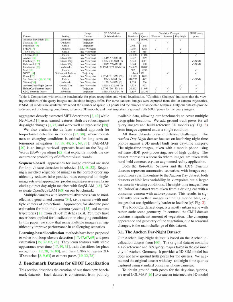
Image 3D SfM Model # Images Condition Changes 6DOF query

Dataset Setting Capture (# Sub-Models) Database Query Weather Seasons Day-Night poses

Alderley Day/Night [48] Suburban Trajectory 14,607 16,960 X X

Nordland [68] Outdoors Trajectory 143k X

Pittsburgh [75] Urban Trajectory 254k 24k

SPED [17] Outdoors Static Webcams 1.27M 120k X X X

Tokyo 24/7 [73] Urban Free Viewpoint 75,984 315 X

7 Scenes [63] Indoor Free Viewpoint 26,000 17,000 X

Aachen [60] Historic City Free Viewpoint 1.54M / 7.28M (1) 3,047 369

Cambridge [32] Historic City Free Viewpoint 1.89M / 17.68M (5) 6,848 4,081 X(SfM)

Dubrovnik [37] Historic City Free Viewpoint 1.89M / 9.61M (1) 6,044 800 X(SfM)

Landmarks [36] Landmarks Free Viewpoint 38.19M / 177.82M (1k) 204,626 10,000

Mall [66] Indoor Free Viewpoint 682 2296 X

NCLT [14] Outdoors & Indoors Trajectory about 3.8M X X

Rome [37] Landmarks Free Viewpoint 4.07M / 21.52M (69) 15,179 1000

San Francisco [16, 36, 59] Urban Free Viewpoint 30M / 149M (1) 610,773 442 X(SfM)

Vienna [30] Landmarks Free Viewpoint 1.12M / 4.85M (3) 1,324 266

Aachen Day-Night (ours) Historic City Free Viewpoint 1.65M / 10.55M (1) 4,328 922 X X

RobotCar Seasons (ours) Urban Trajectory 6.77M / 36.15M (49) 20,862 11,934 X X X X

CMU Seasons (ours) Suburban Trajectory 1.61M / 6.50M (17) 7,159 75,335 X X X

Table 1. Comparison with existing benchmarks for place recognition and visual localization. ”Condition Changes” indicates that the view-

ing conditions of the query images and database images differ. For some datasets, images were captured from similar camera trajectories.

If SfM 3D models are available, we report the number of sparse 3D points and the number of associated features. Only our datasets provide

a diverse set of changing conditions, reference 3D models, and most importantly ground truth 6DOF poses for the query images.

aggregates densely extracted SIFT descriptors [2, 42] while

NetVLAD [1] uses learned features. Both are robust against

day-night changes [1,73] and work well at large-scale [59].

We also evaluate the de-facto standard approach for

loop-closure detection in robotics [23, 38], where robust-

ness to changing conditions is critical for long-term au-

tonomous navigation [17, 39, 48, 51, 69, 73]: FAB-MAP

[20] is an image retrieval approach based on the Bag-of-

Words (BoW) paradigm [65] that explicitly models the co-

occurrence probability of different visual words.

Sequence-based approaches for image retrieval are used

for loop-closure detection in robotics [45, 48, 52]. Requir-

ing a matched sequence of images in the correct order sig-

nificantly reduces false positive rates compared to single-

image retrieval approaches, producing impressive results in-

cluding direct day-night matches with SeqSLAM [48]. We

evaluate OpenSeqSLAM [68] on our benchmark.

Multiple cameras with known relative poses can be mod-

elled as a generalized camera [54], i.e., a camera with mul-

tiple centers of projections. Approaches for absolute pose

estimation for both multi-camera systems [35] and camera

trajectories [11] from 2D-3D matches exist. Yet, they have

never been applied for localization in changing conditions.

In this paper, we show that using multiple images can sig-

nificantly improve performance in challenging scenarios.

Learning-based localization methods have been proposed

to solve both loop-closure detection [17,47,67,69] and pose

estimation [19, 32, 62, 78]. They learn features with stable

appearance over time [17, 49, 51], train classifiers for place

recognition [12, 28, 39, 80], and train CNNs to regress 2D-

3D matches [8, 9, 63] or camera poses [19, 32, 78].

3. Benchmark Datasets for 6DOF Localization

This section describes the creation of our three new bench-

mark datasets. Each dataset is constructed from publicly

available data, allowing our benchmarks to cover multiple

geographic locations. We add ground truth poses for all

query images and build reference 3D models (cf . Fig. 3)

from images captured under a single condition.

All three datasets present different challenges. The

Aachen Day-Night dataset focuses on localizing night-time

photos against a 3D model built from day-time imagery.

The night-time images, taken with a mobile phone using

software HDR post-processing, are of high quality. The

dataset represents a scenario where images are taken with

hand-held cameras, e.g., an augmented reality application.

Both the RobotCar Seasons and the CMU Seasons

datasets represent automotive scenarios, with images cap-

tured from a car. In contrast to the Aachen Day dataset, both

datasets exhibit less variability in viewpoints but a larger

variance in viewing conditions. The night-time images from

the RobotCar dataset were taken from a driving car with a

consumer camera with auto-exposure. This results in sig-

nificantly less well-lit images exhibiting motion blur, i.e.,

images that are significantly harder to localize (cf . Fig. 2).

The RobotCar dataset depicts a mostly urban scene with

rather static scene geometry. In contrast, the CMU dataset

contains a significant amount of vegetation. The changing

appearance and geometry of the vegetation, due to seasonal

changes, is the main challenge of this dataset.

3.1. The Aachen Day­Night Dataset

Our Aachen Day-Night dataset is based on the Aachen lo-

calization dataset from [60]. The original dataset contains

4,479 reference and 369 query images taken in the old inner

city of Aachen, Germany. It provides a 3D SfM model but

does not have ground truth poses for the queries. We aug-

mented the original dataset with day- and night-time queries

captured using standard consumer phone cameras.

To obtain ground truth poses for the day-time queries,

we used COLMAP [61] to create an intermediate 3D model

3

reference model query images

# images # 3D points # features condition conditions (# images)

Aachen Day-Night 4,328 1.65M 10.55M day day (824), night (98)

RobotCar Seasons 20,862 6.77M 36.15M overcast dawn (1,449), dusk (1,182), night (1,314), night+rain (1,320), rain (1,263),

(November) overcast summer / winter (1,389 / 1,170), snow (1,467), sun (1,380)

CMU Seasons 7,159 1.61M 6.50M sun / no foliage sun (22,073), low sun (28,045), overcast (11,383), clouds (14,481),

(April) foliage (33,897), mixed foliage (27,637), no foliage (13,801)

urban (31,250), suburban (13,736), park (30,349)

Table 2. Detailed statistics for the three benchmark datasets proposed in this paper. For each dataset, a reference 3D model was constructed

using images taken under the same reference condition, e.g., ”overcast” for the RobotCar Seasons dataset.

Figure 2. Example query images for Aachen Day-Night (top),

RobotCar Seasons (middle) and CMU Seasons datasets (bottom).

from the reference and day-time query images. The scale of

the reconstruction is recovered by aligning it with the geo-

registered original Aachen model. As in [37], we obtain

the reference model for the Aachen Day-Night dataset by

removing the day-time query images. 3D points visible in

only a single remaining camera were removed as well [37].

The resulting 3D model has 4,328 reference images and

1.65M 3D points triangulated from 10.55M features.

Ground truth for night-time queries. We captured 98

night-time query images using a Google Nexus5X phone

with software HDR enabled. Attempts to include them in

the intermediate model resulted in highly inaccurate camera

poses due to a lack of sufficient feature matches. To obtain

ground truth poses for the night-time queries, we thus hand-

labelled 2D-3D matches. We manually selected a day-time

query image taken from a similar viewpoint for each night-

time query. For each selected day-time query, we projected

its visible 3D points from the intermediate model into it.

Given these projections as reference, we manually labelled

10 to 30 corresponding pixel positions in the night-time

query. Using the resulting 2D-3D matches and the known

intrinsics of the camera, we estimate the camera poses using

a 3-point solver [24, 33] and non-linear pose refinement.

To estimate the accuracy for these poses, we measure the

mean reprojection error of our hand-labelled 2D-3D corre-

spondences (4.33 pixels for 1600x1200 pixel images) and

the pose uncertainty. For the latter, we compute multiple

poses from a subset of the matches for each image and mea-

sure the difference in these poses to our ground truth poses.

The mean median position and orientation errors are 36cm

and 1◦. The absolute pose accuracy that can be achieved by

minimizing a reprojection error depends on the distance of

the camera to the scene. Given that the images were typi-

cally taken 15 or more meters from the scene, we consider

the ground truth poses to be reasonably accurate.

3.2. The RobotCar Seasons Dataset

Our RobotCar Seasons dataset is based on a subset of the

publicly available Oxford RobotCar Dataset [46]. The orig-

inal dataset contains over 20M images recorded from an au-

tonomous vehicle platform over 12 months in Oxford, UK.

Out of the 100 available traversals of the 10km route, we se-

lect one reference traversal in overcast conditions and nine

query traversals that cover a wide range of conditions (cf .

Tab. 2). All selected images were taken with the three syn-

chronized global shutter Point Grey Grasshopper2 cameras

mounted to the left, rear, and right of the car. Both the in-

trinsics of the cameras and their relative poses are known.

The reference traversal contains 26,121 images taken

at 8,707 positions, with 1m between successive positions.

Building a single consistent 3D model from this data is very

challenging, both due to sheer size and the lack of visual

overlap between the three cameras. We thus built 49 non-

overlapping local submaps, each covering a 100m trajec-

tory. For each submap, we initialized the database camera

poses using vehicle positions reported by the inertial nav-

igation system (INS) mounted on the RobotCar. We then

iteratively triangulated 3D points, merged tracks, and re-

fined both structure and poses using bundle adjustment. The

scale of the reconstructions was recovered by registering

them against the INS poses. The reference model contains

all submaps and consists of 20,862 reference images and

6.77M 3D points triangulated from 36.15M features.

We obtained query images by selecting reference posi-

tions inside the 49 submaps and gathering all images from

the nine query traversals with INS poses within 10m of one

of the positions. This resulted in 11,934 images in total,

where triplets of images were captured at 3,978 distinct lo-

cations. We also grouped the queries into 460 temporal se-

quences based on the timestamps of the images.

4

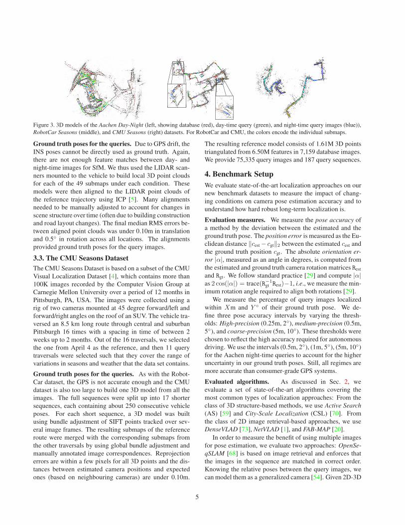
Figure 3. 3D models of the Aachen Day-Night (left, showing database (red), day-time query (green), and night-time query images (blue)),

RobotCar Seasons (middle), and CMU Seasons (right) datasets. For RobotCar and CMU, the colors encode the individual submaps.

Ground truth poses for the queries. Due to GPS drift, the

INS poses cannot be directly used as ground truth. Again,

there are not enough feature matches between day- and

night-time images for SfM. We thus used the LIDAR scan-

ners mounted to the vehicle to build local 3D point clouds

for each of the 49 submaps under each condition. These

models were then aligned to the LIDAR point clouds of

the reference trajectory using ICP [5]. Many alignments

needed to be manually adjusted to account for changes in

scene structure over time (often due to building construction

and road layout changes). The final median RMS errors be-

tween aligned point clouds was under 0.10m in translation

and 0.5◦ in rotation across all locations. The alignments

provided ground truth poses for the query images.

3.3. The CMU Seasons Dataset

The CMU Seasons Dataset is based on a subset of the CMU

Visual Localization Dataset [4], which contains more than

100K images recorded by the Computer Vision Group at

Carnegie Mellon University over a period of 12 months in

Pittsburgh, PA, USA. The images were collected using a

rig of two cameras mounted at 45 degree forward/left and

forward/right angles on the roof of an SUV. The vehicle tra-

versed an 8.5 km long route through central and suburban

Pittsburgh 16 times with a spacing in time of between 2

weeks up to 2 months. Out of the 16 traversals, we selected

the one from April 4 as the reference, and then 11 query

traversals were selected such that they cover the range of

variations in seasons and weather that the data set contains.

Ground truth poses for the queries. As with the Robot-

Car dataset, the GPS is not accurate enough and the CMU

dataset is also too large to build one 3D model from all the

images. The full sequences were split up into 17 shorter

sequences, each containing about 250 consecutive vehicle

poses. For each short sequence, a 3D model was built

using bundle adjustment of SIFT points tracked over sev-

eral image frames. The resulting submaps of the reference

route were merged with the corresponding submaps from

the other traversals by using global bundle adjustment and

manually annotated image correspondences. Reprojection

errors are within a few pixels for all 3D points and the dis-

tances between estimated camera positions and expected

ones (based on neighbouring cameras) are under 0.10m.

The resulting reference model consists of 1.61M 3D points

triangulated from 6.50M features in 7,159 database images.

We provide 75,335 query images and 187 query sequences.

4. Benchmark Setup

We evaluate state-of-the-art localization approaches on our

new benchmark datasets to measure the impact of chang-

ing conditions on camera pose estimation accuracy and to

understand how hard robust long-term localization is.

Evaluation measures. We measure the pose accuracy of

a method by the deviation between the estimated and the

ground truth pose. The position error is measured as the Eu-

clidean distance ‖cest − cgt‖2 between the estimated cest and

the ground truth position cgt. The absolute orientation er-

ror |α|, measured as an angle in degrees, is computed from

the estimated and ground truth camera rotation matrices Rest

and Rgt. We follow standard practice [29] and compute |α|as 2 cos(|α|) = trace(R−1

gt Rest)−1, i.e., we measure the min-

imum rotation angle required to align both rotations [29].

We measure the percentage of query images localized

within Xm and Y ◦ of their ground truth pose. We de-

fine three pose accuracy intervals by varying the thresh-

olds: High-precision (0.25m, 2◦), medium-precision (0.5m,

5◦), and coarse-precision (5m, 10◦). These thresholds were

chosen to reflect the high accuracy required for autonomous

driving. We use the intervals (0.5m, 2◦), (1m, 5◦), (5m, 10◦)

for the Aachen night-time queries to account for the higher

uncertainty in our ground truth poses. Still, all regimes are

more accurate than consumer-grade GPS systems.

Evaluated algorithms. As discussed in Sec. 2, we

evaluate a set of state-of-the-art algorithms covering the

most common types of localization approaches: From the

class of 3D structure-based methods, we use Active Search

(AS) [59] and City-Scale Localization (CSL) [70]. From

the class of 2D image retrieval-based approaches, we use

DenseVLAD [73], NetVLAD [1], and FAB-MAP [20].

In order to measure the benefit of using multiple images

for pose estimation, we evaluate two approaches: OpenSe-

qSLAM [68] is based on image retrieval and enforces that

the images in the sequence are matched in correct order.

Knowing the relative poses between the query images, we

can model them as a generalized camera [54]. Given 2D-3D

5

matches per individual image (estimated via Active Search),

we estimate the pose via a generalized absolute camera

pose solver [35] inside a RANSAC loop. We denote this

approach as Active Search+GC (AS+GC). We mostly use

ground truth query poses to compute the relative poses that

define the generalized cameras1. Thus, AS+GC provides an

upper bound on the number of images that can be localized

when querying with generalized cameras.

The methods discussed above all perform localization

from scratch without any prior knowledge about the pose

of the query. In order to measure how hard our datasets

are, we also implemented two optimistic baselines. Both

assume that a set of relevant database images is known for

each query. Both perform pairwise image matching and use

the known ground truth poses for the reference images to tri-

angulate the scene structure. The feature matches between

the query and reference images and the known intrinsic cal-

ibration are then be used to estimate the query pose. The

first optimistic baseline, LocalSfM, uses upright RootSIFT

features [2, 42]. The second uses upright CNN features

densely extracted on a regular grid. We use the same VGG-

16 network [64] as NetVLAD. The DenseSfM method uses

coarse-to-fine matching with conv4 and conv3 features.

We select the relevant reference images for the two base-

lines as follows: For Aachen, we use the manually selected

day-time image (cf . Sec. 3.1) to select up to 20 reference

images sharing the most 3D points with the selected day-

time photo. For RobotCar and CMU, we use all reference

images within 5m and 135◦ of the ground truth query pose.

We evaluated PoseNet [32] but were not able to obtain

competitive results. We also attempted to train DSAC [8]

on KITTI but were not able to train it. Both PoseNet and

DSAC were thus excluded from further evaluations.

5. Experimental Evaluation

This section presents the second main contribution of this

paper, a detailed experimental evaluation on the effect of

changing conditions on the pose estimation accuracy of vi-

sual localization techniques. In the following, we focus on

pose accuracy. Please see the appendix for experiments con-

cerning computation time.

5.1. Evaluation on the Aachen Day­Night Dataset

The focus of the Aachen Day-Night dataset is on bench-

marking the pose accuracy obtained by state-of-the-art

methods when localizing night-time queries against a 3D

model constructed from day-time imagery. In order to put

the results obtained for the night-time queries into con-

text, we first evaluate a subset of the methods on the 824

day-time queries. As shown in Tab. 3, the two structure-

based methods are able to estimate accurate camera poses

1Note that Active Search+GC only uses the relative poses between the

query images to define the geometry of a generalized camera. It does not

use any information about the absolute poses of the query images.

NetVLADDenseVLAD

FABMAPAS

CSLDenseSfM

LocalSfMseqSLAM

CSL-subAS+GC(seq)

0 5 10 15 20Distance threshold [m]

0%

20%

40%

60%

80%

100%

correctly lo

calized

que

ries

0 5 10 15 20Distance threshold [m]

0%

10%

20%

30%

40%

50%

correctly lo

calized

que

ries

Figure 4. Cumulative distribution of position errors for the night-

time queries of the Aachen (left) and RobotCar (right) datasets.

and localize nearly all images within the coarse-precision

regime. We conclude that the Aachen dataset is not partic-

ularly challenging for the day-time query images.

Night-time queries. Tab. 3 also reports the results obtained

for the night-time queries. We observe a significant drop in

pose accuracy for both Active Search and CSL, down from

above 50% in the high-precision regime to less than 50%

in the coarse-precision regime. Given that the night-time

queries were taken from similar viewpoints as the day-time

queries, this drop is solely caused by the day-night change.

CSL localizes more images compared to Active Search

(AS). This is not surprising since CSL also uses matches

that were rejected by AS as too ambiguous. Still, there is a

significant difference to LocalSfM. CSL and AS both match

features against the full 3D model while LocalSfM only

considers a small part of the model for each query. This

shows that global matching sufficiently often fails to find

the correct nearest neighbors, likely caused by significant

differences between day-time and night-time descriptors.

Fig. 4(left) shows the cumulative distribution of position

errors for the night-time queries and provides interesting in-

sights: LocalSfM, despite knowing relevant reference im-

ages for each query, completely fails to localize about 20%

of all queries. This is caused by a lack of correct feature

matches for these queries, either due to failures of the fea-

ture detector or descriptor. DenseSfM skips feature detec-

tion and directly matches densely extracted CNN descrip-

tors (which encode higher-level information compared to

the gradient histograms used by RootSIFT). This enables

DenseSfM to localize more images at a higher accuracy, re-

sulting in the best performance on this dataset. Still, there

is significant room for improvement, even in the coarse-

precision regime (cf . Tab. 3). Also, extracting and matching

dense descriptors is a time-consuming task.

5.2. Evaluation on the RobotCar Seasons Dataset

The focus of the RobotCar Seasons dataset is to measure

the impact of different seasons and illumination conditions

on pose estimation accuracy in an urban environment.

Tab. 4 shows that changing day-time conditions have

only a small impact on pose estimation accuracy for all

methods. The reason is that seasonal changes have little im-

6

Aachen CMU

day night foliage mixed foliage no foliage urban suburban park

m

deg

.25/.50/5.0

2/5/10

0.5/1.0/5.0

2/5/10

.25/.50/5.0

2/5/10

.25/.50/5.0

2/5/10

.25/.50/5.0

2/5/10

.25/.50/5.0

2/5/10

.25/.50/5.0

2/5/10

.25/.50/5.0

2/5/10

Active Search 57.3 / 83.7 / 96.6 19.4 / 30.6 / 43.9 28.8 / 32.5 / 35.9 25.1 / 29.4 / 33.9 52.5 / 59.4 / 66.7 55.2 / 60.3 / 65.1 20.7 / 25.9 / 29.9 12.7 / 16.3 / 20.8

CSL 52.3 / 80.0 / 94.3 24.5 / 33.7 / 49.0 16.3 / 19.1 / 26.0 15.2 / 18.8 / 28.6 36.5 / 43.2 / 57.5 36.7 / 42.0 / 53.1 8.6 / 11.7 / 21.1 7.0 / 9.6 / 17.0

DenseVLAD 0.0 / 0.1 / 22.8 0.0 / 2.0 / 14.3 13.2 / 31.6 / 82.3 16.2 / 38.1 / 85.4 17.8 / 42.1 / 91.3 22.2 / 48.7 / 92.8 9.9 / 26.6 / 85.2 10.3 / 27.0 / 77.0

NetVLAD 0.0 / 0.2 / 18.9 0.0 / 2.0 / 12.2 10.4 / 26.1 / 80.1 11.0 / 26.7 / 78.4 11.8 / 29.1 / 82.0 17.4 / 40.3 / 93.2 7.7 / 21.0 / 80.5 5.6 / 15.7 / 65.8

FABMAP 0.0 / 0.0 / 4.6 0.0 / 0.0 / 0.0 1.1 / 2.7 / 16.5 1.0 / 2.5 / 14.7 3.6 / 7.9 / 30.7 2.7 / 6.4 / 27.3 0.5 / 1.5 / 13.6 0.8 / 1.7 / 11.5

LocalSfM 36.7 / 54.1 / 72.4 55.4 / 57.0 / 59.9 52.4 / 55.1 / 58.6 70.8 / 72.7 / 75.9 72.8 / 74.1 / 76.1 55.2 / 57.7 / 61.3 41.8 / 44.5 / 48.7

DenseSfM 39.8 / 60.2 / 84.7

AS+GC(seq) 86.6 / 93.0 / 99.3 76.3 / 88.5 / 99.8 77.6 / 86.8 / 99.8 86.4 / 93.6 / 99.8 92.0 / 96.0 / 99.7 71.0 / 84.0 / 99.2

Table 3. Evaluation on the Aachen Day-Night dataset and a subset of the conditions of the CMU Seasons dataset.

day conditions night conditions

dawn dusk OC-summer OC-winter rain snow sun night night-rain

m

deg

.25 / .50 / 5.0

2 / 5 / 10

.25 / .50 / 5.0

2 / 5 / 10

.25 / .50 / 5.0

2 / 5 / 10

.25 / .50 / 5.0

2 / 5 / 10

.25 / .50 / 5.0

2 / 5 / 10

.25 / .50 / 5.0

2 / 5 / 10

.25 / .50 / 5.0

2 / 5 / 10

.25 / .50 / 5.0

2 / 5 / 10

.25 / .50 / 5.0

2 / 5 / 10

ActiveSearch 36.2 / 68.9 / 89.4 44.7 / 74.6 / 95.9 24.8 / 63.9 / 95.5 33.1 / 71.5 / 93.8 51.3 / 79.8 / 96.9 36.6 / 72.2 / 93.7 25.0 / 46.5 / 69.1 0.5 / 1.1 / 3.4 1.4 / 3.0 / 5.2

CSL 47.2 /73.3 / 90.1 56.6 / 82.7 / 95.9 34.1 / 71.1 / 93.5 39.5 / 75.9 / 92.3 59.6 / 83.1 / 97.6 53.2 / 83.6 / 92.4 28.0 / 47.0 / 70.4 0.2 / 0.9 / 5.3 0.9 / 4.3 / 9.1

DenseVLAD 8.7 / 36.9 / 92.5 10.2 / 38.8 / 94.2 6.0 / 29.8 / 92.0 4.1 / 26.9 / 93.3 10.2 / 40.6 / 96.9 8.6 / 30.1 / 90.2 5.7 / 16.3 / 80.2 0.9 / 3.4 / 19.9 1.1 / 5.5 / 25.5

NetVLAD 6.2 / 22.8 / 82.6 7.4 / 29.7 / 92.9 6.5 / 29.6 / 95.2 2.8 / 26.2 / 92.6 9.0 / 35.9 / 96.0 7.0 / 25.2 / 91.8 5.7 / 16.5 / 86.7 0.2 / 1.8 / 15.5 0.5 / 2.7 / 16.4

FABMAP 1.2 / 5.6 / 14.9 4.1 / 18.3 / 55.1 0.9 / 8.9 / 39.3 2.6 / 13.3 / 44.1 8.8 / 32.1 / 86.5 2.0 / 8.2 / 28.4 0.0 / 0.0 / 2.4 0.0 / 0.0 / 0.0 0.0 / 0.0 / 0.0

Table 4. Evaluation on the RobotCar Seasons dataset. We report the percentage of queries localized within the three thresholds.

all day all night

m

deg

.25 / .50 / 5.0

2 / 5 / 10

.25 / .50 / 5.0

2 / 5 / 10

ActiveSearch 35.6 / 67.9 / 90.4 0.9 / 2.1 / 4.3

CSL 45.3 / 73.5 / 90.1 0.6 / 2.6 / 7.2

ActiveSearch+GC (triplet) 45.5 / 77.0 / 94.7 2.7 / 6.9 / 12.1

ActiveSearch+GC (sequence, GT) 46.7 / 80.1 / 97.0 5.8 / 21.0 / 43.1

seqSLAM 1.3 / 6.1 / 15.3 0.2 / 0.7 / 1.5

Table 5. Using multiple images for pose estimation (Ac-

tiveSeach+GC) on the RobotCar Seasons dataset.

pact on the building facades that are dominant in most query

images. The exceptions are “dawn” and “sun”. For both,

we observed overexposed images caused by direct sunlight

(cf . Fig. 1). Thus, fewer features can be found for Active

Search and CSL and the global image descriptors used by

the image retrieval approaches are affected as well.

On the Aachen Day-Night dataset, we observed that im-

age retrieval-based methods (DenseVLAD and NetVLAD)

consistently performed worse than structure-based methods

(Active Search, CSL, LocalSfM, and DenseSfM). For the

RobotCar dataset, NetVLAD and DenseVLAD essentially

achieve the same coarse-precision performance as Active

Search and CSL. This is caused by the lower variation in

viewpoints as the car follows the same road.

Compared to Aachen, there is an even stronger drop

in pose accuracy between day and night for the RobotCar

dataset. All methods fail to localize a significant num-

ber of queries for both the high- and medium-precision

regimes. Interestingly, DenseVLAD and NetVLAD out-

perform all other methods in the coarse-precision regime

(cf . Fig. 4(right)). This shows that their global descrip-

tors still encode distinctive information even if local fea-

ture matching fails. The better performance of all methods

under ”night+rain” compared to ”night” comes from the au-

toexposure of the RobotCar’s cameras. A longer exposure

is used for the ”night”, leading to significant motion blur.

Multi-image queries. The RobotCar is equipped with

RobotCar - all night

m

deg

.25 / .50 / 5.0

2 / 5 / 10

ActiveSearchfull model 0.9 / 2.1 / 4.3

sub-model 3.2 / 7.9 / 12.0

CSLfull model 0.6 / 2.6 / 7.2

sub-model 0.5 / 2.8 / 13.4

ActiveSearch+GC (triplet)full model 2.7 / 6.9 / 12.1

sub-model 7.4 / 15.3 / 27.0

ActiveSearch+GC (sequence, GT)full model 5.8 / 21.0 / 43.1

sub-model 13.3 / 35.9 / 61.8

ActiveSearch+GC (sequence, VO)full model 1.5 / 7.4 / 22.9

sub-model 3.6 / 12.5 / 42.2

LocalSfM sub-model 16.1 / 27.3 / 44.1

Table 6. Using location priors to query only submodels rather

than the full RobotCar Seasons dataset for night-time queries.

three synchronized cameras and captures sequences of im-

ages for each camera. Rather than querying with only a

single image, we can thus also query with multiple photos.

Tab. 5 shows the results obtained with seqSLAM (which

uses temporal sequences of all images captured by the three

cameras) and Active Search+GC. For the latter, we query

with triplets of images taken at the same time as well as

with temporal sequences of triplets. For the triplets, we use

the known extrinsic calibration between the three cameras

mounted on the car. For the temporal sequences, we use

relative poses obtained from the ground truth (GT) absolute

poses. For readability, we only show the results summarized

for day- and night-conditions.

Tab. 5 shows that Active Search+GC consistently out-

performs single image methods in terms of pose accuracy.

Active Search+GC is able to accumulate correct matches

over multiple images. This enables Active Search+GC to

succeed even if only a few matches are found for each in-

dividual image. Naturally, the largest gain can be observed

when using multiple images in a sequence.

Location priors. In all previous experiments, we consid-

ered the full RobotCar 3D model for localization. How-

ever, it is not uncommon in outdoor settings to have a rough

7

prior on the location at which the query image was taken.

We simulate such a prior by only considering the sub-model

relevant to a query rather than the full model. While we ob-

serve only a small improvement for day-time queries, local-

izing night-time queries significantly benefits from solving

an easier matching problem (cf . Tab. 6). For completeness,

we also report results for LocalSfM, which also considers

only a small part of the model relevant to a query. Active

Search+GC outperforms LocalSfM on this easier matching

task when querying with sequences. This is due to not rely-

ing on one single image to provide enough matches.

One drawback of sequence-based localization is that the

relative poses between the images in a sequence need to be

known quite accurately. Tab. 6 also reports results obtained

when using our own multi-camera visual odometry (VO)

system to compute the relative poses. While performing

worse compared to ground truth relative poses, this more

realistic baseline still outperforms methods using individual

images. The reasons for the performance drop are drift and

collapsing trajectories due to degenerate configurations.

5.3. Evaluation on the CMU Seasons Dataset

Compared to the urban scenes shown in the other datasets,

significant parts of the CMU Seasons dataset show suburban

or park regions. Seasonal changes can drastically affect the

appearance of such regions. In the following, we thus focus

on these conditions (see the appendix for an evaluation of

all conditions). For each query image, we only consider its

relevant sub-model.

Tab. 3 evaluates the impact of changes in foliage and of

different regions on pose accuracy. The reference condi-

tion for the CMU Seasons dataset does not contain foliage.

Thus, other conditions for which foliage is also absent lead

to the most accurate poses. Interestingly, DenseVLAD and

NetVLAD achieve a better performance than Active Search

and CSL for the medium- and coarse-precision regimes un-

der the ”Foliage” and ”Mixed Foliage” conditions. For the

coarse-precision regime, they even outperform LocalSfM.

This again shows that global image-level descriptors can

capture information lost by local features.

We observe a significant drop in pose accuracy in both

suburban and park regions. This is caused by the dominant

presence of vegetation, leading to many locally similar (and

thus globally confusing) features. LocalSfM still performs

well as it only considers a few reference images that are

known to be a relevant for a query image. Again, we notice

that DenseVLAD and NetVLAD are able to coarsely local-

ize more queries compared to the feature-based methods.

Localizing sequences (Active Search+GC) again dras-

tically helps to improve pose estimation accuracy. Com-

pared to the RobotCar Seasons dataset, where the sequences

are rather short (about 20m maximum), the sequences used

for the CMU Seasons dataset completely cover their cor-

responding sub-models. In practical applications, smaller

sequences are preferable to avoid problems caused by drift

when estimating the relative poses in a sequence. Still, the

results from Tab. 3 show the potential of using multiple

rather than a single image for camera pose estimation.

6. Conclusion & Lessons Learned

In this paper, we have introduced three challenging new

benchmark datasets for visual localization, allowing us, for

the first time, to analyze the impact of changing conditions

on the accuracy of 6DOF camera pose estimation. Our ex-

periments clearly show that the long-term visual localiza-

tion problem is far from solved.

The extensive experiments performed in this paper lead

to multiple interesting conclusions: (i) Structure-based

methods such as Active Search and CSL are robust to

most viewing conditions in urban environments. Yet, per-

formance in the high-precision regime still needs to be

improved significantly. (ii) Localizing night-time images

against a database built from day-time photos is a very

challenging problem, even when a location prior is given.

(iii) Scenes with a significant amount of vegetation are chal-

lenging, even when a location prior is given. (iv) SfM, typ-

ically used to obtain ground truth for localization bench-

marks, does not fully handle problems (ii) and (iii) due

to limitations of existing local features. Dense CNN fea-

ture matching inside SfM improves pose estimation per-

formance at high computational costs, but does not fully

solve the problem. Novel (dense) features, e.g., based

on scene semantics [62], seems to be required to solve

these problems. Our datasets readily provide a benchmark

for such features through the LocalSfM and DenseSfM

pipelines. (v) Image-level descriptors such as DenseVLAD

can succeed in scenarios where local feature matching fails.

They can even provide coarse-level pose estimates in au-

tonomous driving scenarios. Aiming to improve pose ac-

curacy, e.g., by denser view sampling via synthetic im-

ages [73] or image-level approaches for relative pose es-

timation, is an interesting research direction. (vi) There is a

clear benefit in using multiple images for pose estimation.

Yet, there is little existing work on multi-image localization.

Fully exploiting the availability of multiple images (rather

than continuing the focus on single images) is thus another

promising avenue for future research.

Acknowledgements. This work was partially supported by

ERC grant LEAP No. 336845, CIFAR Learning in Machines

& Brains program, EU-H2020 project LADIO 731970, the

European Regional Development Fund under the project IM-

PACT (reg. no. CZ.02.1.01/0.0/0.0/15 003/0000468), JSPS

KAKENHI Grant Number 15H05313, EPSRC Programme Grant

EP/M019918/1, the Swedish Research Council (grant no. 2016-

04445), the Swedish Foundation for Strategic Research (Semantic

Mapping and Visual Navigation for Smart Robots), and Vinnova /

FFI (Perceptron, grant no. 2017-01942).

8

Appendix

This appendix provides additional results, in particular eval-

uations under all conditions on the CMU Seasons dataset

and run-time results for the evaluated methods. In addition,

a more detailed description of the state-of-the-art localiza-

tion approaches evaluated in the paper is provided. This

includes details on the parameter settings used in our exper-

iments, which are provided to foster reproducibility.

The appendix is structured as follows: Sec. A provides

a more detailed description of all evaluated state-of-the-

art approaches. Sec. B provides additional details for the

RobotCar Seasons and CMU Seasons datasets. Sec. C

provides timing results for these methods on the different

datasets. Sec. D shows evaluation results on the CMU Sea-

sons under all conditions. Finally, Sec. E shows the cumu-

lative distributions in position and orientation error for all

state-of-the-art methods evaluated on our benchmark.

A. Details on the Evaluated Algorithms

This section provides a detailed description, including pa-

rameter settings, of the state-of-the-art algorithms used for

experimental evaluation (cf . Sec. 5 in the paper).

A.1. 3D Structure­based Localization

Active Search (AS). Active Search [58] accelerates 2D-3D

descriptor matching via a prioritization scheme. It uses a vi-

sual vocabulary to quantize the descriptor space. For each

query feature, it determines how many 3D point descrip-

tors are assigned to the feature’s closest visual word. This

determines the number of descriptor comparisons needed

for matching this feature. Active Search then matches the

features in ascending order of the number of required de-

scriptor comparisons. If a 2D-to-3D match is found, Ac-

tive Search attempts to find additional 3D-to-2D correspon-

dences for the 3D points surrounding the matching point.

Correspondence search terminates once 100 matches have

been found.

For the Aachen Day-Night dataset, we trained a visual

vocabulary containing 100k words using approximate k-

means clustering [53] on all upright RootSIFT [2, 42] de-

scriptors found in 1,000 randomly selected database images

contained in the 3D model. Similarly, we trained a vocabu-

lary containing 10k words for the RobotCar Seasons dataset

from the descriptors found in 1,000 randomly selected im-

ages contained in the reference 3D model. For the CMU

Seasons dataset, we also trained a visual vocabulary con-

sisting of 10k words, but used the SIFT [42] features cor-

responding to the 3D points in all sub-models instead of

RootSIFT features. No vocabulary contains any informa-

tion from the query images.

We use calibrated cameras rather than simultaneously es-

timating each camera’s extrinsic and intrinsic parameters.

We thereby exploit the known intrinsic calibrations pro-

vided by the intermediate model of the Aachen Day-Night

dataset2 and the known intrinsics of the RobotCar Seasons

and CMU Seasons datasets.

Besides training new vocabularies and using calibrated

cameras, we only changed the threshold on the re-projection

error used by RANSAC to distinguish between inliers and

outliers. For the Aachen Day-Night dataset, we used a

threshold of 10 pixels while we used 5 pixels for both the

RobotCat Seasons and the CMU Seasons datasets. Other-

wise, we used the standard parameters of Active Search.

City-Scale Localization (CSL). The City-Scale Localiza-

tion algorithm [70] is an outlier rejection algorithm, i.e., it

is a robust localization algorithm that can prune guaranteed

outlier correspondences from a given set of 2D-3D corre-

spondences. CSL is based on the following central insight:

If the gravity direction and an approximate height of the

camera above the ground plane are known, it is possible to

calculate an upper bound for the maximum number of in-

liers that any solution containing a given 2D-3D correspon-

dence as an inlier can have. At the same time, CSL also

computes a lower bound on the number of inliers for a given

correspondence by computing a pose for which this corre-

spondence is an inlier. CSL thus computes this upper bound

for each 2D-3D match and, similar to RANSAC, continu-

ously updates the best pose found so far (which provides a

lower bound on the number of inliers that can be found).

All correspondences with an upper bound on the maximum

number of inliers that is below the number of inliers in the

current best solution can be permanently discarded from

further consideration. When outliers have been discarded,

three-point RANSAC [24, 33] is performed on the remain-

ing correspondences. Notice that, unlike RANSAC, the out-

lier filter used by CSL is deterministic. The computational

complexity of the filter is O(N2 logN), where N is the

number of available 2D-3D correspondences.

In order to obtain an estimate for the gravity direction,

we follow [70] and add noise to the gravity direction ob-

tained from the ground truth poses. CSL iterates over a

range of plausible height values, similar to [81]. In these

experiments, the height values cover an interval five meters

high. This interval is centered on the camera height of the

ground truth pose, with added noise. In the Aachen experi-

ments, the height interval is divided into nine sections, and

for the Oxford and CMU experiments, the height interval is

divided into three sections.

The 2D-3D correspondences are generated by matching

the descriptors of all detected features in the query image

to the descriptors of the 3D points using approximate near-

2Some of the day-time queries were taken with the same camera as the

night-time queries and we enforced that the images taken with the same

camera have consistent intrinsics. Thus, the intermediate model provides

the intrinsic calibration of the night-time queries.

9

Parameter Value

Feature Type Dense RootSIFT

Vocabulary Size 128

(trained on SF)

Descriptor Dimension 4,096

(after PCA & whitening)Table 7. DenseVLAD parameters.

Parameter Value

Network model VGG-16 + NetVLAD

(trained on Pitts30k) + whitening

Descriptor Dimension 4,096Table 8. NetVLAD parameters.

est neighbour search. To account for the fact that each 3D

point is associated with multiple descriptor, the 3D points

are each assigned a single descriptor vector equal to the

mean of all its corresponding descriptors. This matching

strategy yields the same number of correspondences as the

number of detected features.

As with Active Search, we use a re-projection error

threshold of 10 pixels for the Aachen Day-Night dataset and

5 pixels for both the RobotCat Seasons and the CMU Sea-

sons datasets.

A.2. 2D Image­based Localization

DenseVLAD and NetVLAD. We use the original imple-

mentations of DenseVLAD [74] and NetVLAD [1] pro-

vided by the authors. Images were processed at their orig-

inal resolution unless any dimension exceeded 1920 pix-

els. For DenseVLAD, we used the Dense SIFT imple-

mentation, followed by RootSIFT normalization [2], avail-

able in VLFeat [77]. The visual vocabulary used consisted

of 128 visual words (centroids) pre-computed on the San-

Francisco (SF) dataset [15], i.e., we used a general vo-

cabulary trained on a different yet similiar dataset. For

NetVLAD we used the pre-computed network “Pitts30k”

trained on the Pittsburgh time-machine street-view image

dataset [1]. The network is therefore not fine-tuned on our

datasets, i.e., we again used a general network trained on a

different city.

Given a DenseVLAD or NetVLAD descriptor, we find

the most similar reference image by exhaustive nearest

neighbor search. While this stage could be accelerated by

approximate search, we found this to be unnecessary as the

search for a single query descriptor typically takes less than

20ms.

Tables 7 and 8 summarize the parameters used for Den-

seVLAD and NetVLAD in our experiments.

FAB-MAP. For FAB-MAP [20], we trained a separate vo-

cabulary for each location using Modified Sequential Clus-

tering [72] on evenly spaced database images, resulting in

3,585 visual words for Aachen Day-Night, 5,031 for Robot-

Car Seasons and 4,847 for CMU Seasons. A Chow-Liu tree

Parameter Value

Feature Type UprightSURF128

Aachen Vocabulary Size 3585

RobotCar Vocabulary Size 5031

CMU Vocabulary Size 4847

p (zi | ei) 0

p (zi | ei) 0.61

p(

Lnew | Zk−1)

0.9Table 9. FAB-MAP parameters.

was built for each dataset using the Bag-of-Words generated

for each database image using the vocabulary. We used the

mean field approximation for the new place likelihood (as

additional training images were not available for the sam-

pled approach used in [21]) and the fast lookup-table im-

plementation in [27] to perform image retrieval for each of

the query locations. Tab. 9 summarizes the parameters used

for the experiments.

A.3. Optimistic Baselines

As explained in Sec. 5 of the paper, we implemented two

optimistic baselines. Whereas all other localization algo-

rithms evaluated in the paper use no prior information on

a query image’s pose, both optimistic baselines are given

additional knowledge. For each query image, we provide a

small set of reference images depicting the same part of the

model. The remaining problem is to establish sufficiently

many correspondences between the query and the selected

reference images to facilitate camera pose estimation. Thus,

both approaches measure an upper bound on the pose qual-

ity that can be achieved with a given type of local feature.

LocalSfM. Given a query image and its relevant set of

reference images, LocalSfM first extracts upright Root-

SIFT [2, 42] features. Next, LocalSfM performs exhaustive

feature matching between the relevant reference images as

well as between the query and the relevant reference im-

ages. While Active Seach and CSL both use Lowe’s ratio

test3, DenseSfM neither uses the ratio test nor a threshold on

the maximum descriptor distance. Instead, it only requires

matching features to be mutual nearest neighbors. Given

the known poses and intrinsics for the reference images, Lo-

calSfM triangulates the 3D structure of the scene using the

previously established 2D-2D matches. Notice that the re-

sulting 3D model is automatically constructed in the global

coordinate system of the reference 3D model. Finally, we

use the known intrinsics of the query image and the feature

matches between the query and the reference images to es-

timate the camera pose of the query.

For each query image, the relevant set of reference im-

ages is selected as follows: For the RobotCar Seasons and

CMU Seasons datasets, we use the ground truth pose of

3Active Search uses a ratio test threshold of 0.7 for 2D-to-3D and a

threshold of 0.6 for 3D-to-2D matching.

10

each query image to identify a relevant set of reference im-

ages. More precisely, we select all reference images whose

camera centers are within 5m of the ground truth position

of the query and whose orientations are within 135◦ of the

orientation of the query image.

As explained in Sec. 3.2 of the paper, we manually se-

lect a day-time query image taken from a similar viewpoint

for each nigh-time query photo in the Aachen Day-Night

dataset. The day-time queries were included when con-

structing the intermediate model. Thus, their ground truth

poses as well as a set of 3D points visible in each of them are

obtain from the intermediate Structure-from-Motion model.

For each day-time query, we select up to 20 reference im-

ages that observe the largest number of the 3D points visible

in the day-time query. These reference images then form

the set of relevant images for the corresponding night-time

query photo.

LocalSfM is implemented using COLMAP [61]. It is

rather straight-forward to replace upright RootSIFT features

with other types of local features. In order to encourage the

use of our benchmark for the evaluation of local features,

we will make our implementation publicly available.

DenseSfM. DenseSfM modifies the LocalSfM approach

by replacing RootSIFT [2] features extracted at DoG ex-

trema [42] with features densely extracted from a regu-

lar grid [7, 40]. The goal of this approach is to increase

the robustness of feature matching between day- and night-

time images [74, 82]. We used convolutional layers (conv4

and conv3) from a VGG-16 network [64], which was pre-

trained as part of the NetVLAD model (Pitts30k), as fea-

tures. We generated tentative correspondences by matching

the extracted features in a coarse-to-fine manner: We first

match conv4 features and use the resulting matches to re-

strict the correspondence search for conv3 features. As for

LocalSfM, we performed exhaustive pairwise image match-

ing. The matches are verified by estimating up to two homo-

graphies between each image pair via RANSAC [24]. The

resulting verified feature matches are then used as input for

COLMAP [61]. The reconstruction process is the same as

for LocalSfM, i.e., we first triangulate the 3D points and

then use them to estimate the pose of the night-time query.

DenseSfM uses the same set of reference images for each

query photo as LocalSfM.

A.4. Localization from Multiple Images

Active Search + Generalized Cameras (Active

Search+GC). While most existing work on visual

localization focuses on estimating the camera pose of

an individual single query image, this paper additionally

evaluates the benefits of using multiple images simul-

taneously for pose estimation. To this end, we assume

that the relative poses between multiple query images are

known and model these multiple images as a generalized

camera. Given the matches found via Active Search for

each individual image in a generalized camera, we use

the 3-point-generalized-pose (GP3P) solver from [35] to

estimate the pose of the generalized camera. Together

with the known relative poses, this provides us with a pose

for each image in the generalized camera. We use these

individual poses to evaluate the pose estimation accuracy.

An inlier threshold of 12 pixels is used by RANSAC.

Active Search+GC is not evaluated on the Aachen Day-

Night dataset as it only provides individual query images.

For the RobotCar Seasons, we evaluate two variants: Ac-

tive Search+GC (triplet) builds a generalized camera from

images captured at the same point in time by the three cam-

eras mounted on the RobotCar (left, rear, right). The result-

ing generalized cameras thus consist of three images each.

Active Search+GC (sequence) uses longer sequences taken

with all three cameras. Each sequence consists of images

taken consecutively in time under the same condition. More

specifically, each sequence consists of a temporal sequence

of images taken around the 49 manually selected reference

positions (cf . Sec. 3.2 in the paper). For the CMU Seasons

dataset, we only evaluate the Active Search+GC (sequence).

All query images taken under the same condition for a given

sub-model define one sequence.

In order to use the GP3P solver, the relative poses be-

tween the images in a generalized camera, as well as the

scale of the relative translations between the images, need to

be known. In our experiments, we extract the required rela-

tive poses directly from the ground truth camera poses. As

a consequence, the results obtained with Active Search+GC

(sequence) are optimistic in the sense that the method does

not need to deal with the drift that normally occurs when

estimating a trajectory via SLAM or SfM. Notice that we

only use the relative poses. No information about the ab-

solute pose of a generalized camera is used during pose

estimation. Also, notice that the results obtained for Ac-

tive Search+GC (triplet) are realistic: In this case, we are

only using the known extrinsic calibration between the three

cameras mounted on the RobotCar to define each general-

ized camera.

We also experimented with relative poses generated by

our own multi-camera visual odometry (VO) system. Tab. 6

in the paper compares the results obtained when using

ground truth poses with those obtained when using poses

estimated by our VO pipeline on the night-time images of

the RobotCar Seasons dataset. As can be seen, using ground

truth poses leads to better results as generalized camera pose

solvers are typically sensitive to calibration errors. Still, Ac-

tive Search+GC with VO poses outperforms single image-

based methods. We also evaluated Active Search+GC (se-

quence) on the CMU datasets, but found that the drift in the

odometry was too severe to provide accurate camera poses.

11

Parameter Value

Image Size 48× 48 (144× 48)

Patch Size 8× 8Sequence Length ds 10

Table 10. SeqSLAM parameters.

# images

condition recorded individual triplets sequences

overcast (reference) 28 Nov 2014 20,862 8,707 -

dawn 16 Dec 2014 1,449 483 54

dusk 20 Feb 2015 1,182 394 48

night 10 Dec 2014 1,314 438 49

night+rain 17 Dec 2014 1,320 440 51

overcast (summer) 22 May 2015 1,389 463 52

overcast (winter) 13 Nov 2015 1,170 390 49

rain 25 Nov 2014 1,263 421 50

snow 3 Feb 2015 1,467 489 56

sun 10 Mar 2015 1,380 460 51

total query - 11,934 3,978 460

Table 11. Detailed statistics for the RobotCar Seasons dataset. We

used images from the overcast (reference) traversal to build a 3D

scene model. For each of the query sequences, we report the total

number of query images taken by all three individual cameras, the

resulting number of triplets used for Active Search+GC (triplet),

and the number of temporally continuous query sequences used

for Active Search+GC (sequence).

An interesting experiment would be to use only short sub-

sequences (for which the drift is not too large) rather than

the full sequences.

SeqSLAM. We used the OpenSeqSLAM implementation

from [68] with default parameters for template learning

and trajectory uniqueness. For each set of synchronized

Grasshopper2 images, we downscale the original 1024 ×1024 resolution to 48 × 48, then concatenate all three im-

ages to form a 144 × 48 pixel composite. The trajectory

length parameter ds was set to 10 images; as both the query

and database images are evenly spaced this corresponds to

a trajectory length of 10 meters. Tab. 10 summarizes the

parameters used for the RobotCar experiments.

B. Dataset Details

This section provides additional details for the RobotCar

Seasons and CMU Seasons dataset. More specifically,

Tab. 11 details the time at which the individual traversals

were recorded, the number of images per traversal, as well

as the number of triplets and sequences used for Active

Search+GC. Tab. 12 provides similar details for the CMU

Seasons dataset. In addition to listing the conditions for the

different recordings, Tab. 13 lists the respective scenery (ur-

ban, suburban and park) for the different sub-models.

C. Timing Results

Tab. 14 provides an overview over the run-times of the var-

ious methods used for experimental evaluation on the three

# images

condition recorded individual sequences

Sunny + No Foliage (reference) 4 Apr 2011 7,159 17

Sunny + Foliage 1 Sep 2010 8,076 16

Sunny + Foliage 15 Sep 2010 7,260 17

Cloudy + Foliage 1 Oct 2010 7,185 17

Sunny + Foliage 19 Oct 2010 6,737 17

Overcast + Mixed Foliage 28 Oct 2010 6,744 17

Low Sun + Mixed Foliage 3 Nov 2010 6,982 17

Low Sun + Mixed Foliage 12 Nov 2010 7,262 17

Cloudy + Mixed Foliage 22 Nov 2010 6,649 17

Low Sun + No Foliage + Snow 21 Dec 2010 6,825 17

Low Sun + No Foliage 4 Mar 2011 6,976 17

Overcast + Foliage 28 Jul 2011 4,639 17

total query - 75,335 186

Table 12. Detailed statistics for the CMU Seasons dataset. We used

images from the reference traversal to build a 3D scene model. For

each of the query sequences, we report the total number of query

images taken and the number of temporally continuous query se-

quences used for Active Search+GC (sequence).

Scene Sub-model # images

Urban 1 - 7 31,250

Suburban 8 - 10 13,736

Park 11 - 17 30,349

total query - 75,335

Table 13. The type of scenery (urban, suburban and park) depicted

in the different sub-models of the CMU Seasons dataset and the to-

tal number of query images for each type. In total there are 31,250

urban, 13,736 suburban and 30,349 park images.

benchmark datasets. Timings are given in seconds and do

include feature matching and (if applicable) camera pose

estimation. However, feature extraction times are not in-

cluded in the run-times since most algorithms are indepen-

dent of the underlying feature representation and, in exten-

sion thereof, the specific implementation used to extract the

features.

We ran the different algorithms on different machines.

For all variants of Active Search, a PC with an Intel Core

i7-4770 CPU with 3.4GHz, 32GB of RAM, and an NVidia

GeForce GTX 780 GPU was used. The same machine was

used to run LocalSfM. Notice that due to their need to match

multiple images, most of the run-time of Active Search+GC

and LocalSfM is spent on feature matching. The increase in

run-time for LocalSfM from the Aachen Day-Night to the

RobotCar Seasons and CMU Seasons datasets is caused by

the number of reference images considered for each dataset.

For Aachen Day-Night, at most 20 reference images are

considered per query while more images are used on the

other two datasets (where more reference images are used

for the CMU dataset due to a higher sampling density of

the reference images). CSL was run on a computer clus-

ter using an Intel Xeon E5-2650 v3 with 3.2 GB RAM

per CPU core. The fact that CSL is substantially slower

on the Aachen Day-Night dataset than on the RobotCar

Seasons and CMU Seasons datasets is due to the image

12

Aachen Day-Night RobotCar Seasons CMU Seasons

Day Night

Method Day Night full model sub-models full model sub-models All

Active Search 0.102 0.140 0.291 0.061 0.973 0.093 0.065

CSL 168.6 206.2 32.9 90.3† 66.3 90.3

† 30.7

DenseVLAD * 0.752 0.527 0.338 - 0.338 - 0.785

NetVLAD ⋄ 0.105 0.105 0.137 - 0.137 - 0.107

FABMAP 0.008 0.008 0.039 - 0.039 - 0.013

Active Search+GC (triplet) - - 0.879 0.180 2.940 0.289 -

Active Search+GC (sequence) - - 1.570 0.317 5.267 0.515 26.278

seqSLAM - - 0.251 - 0.251 - -

LocalSfM *,⋄ - 19.591 - 22.486 44.577

DenseSfM * - 16.719 - - - - -

Table 14. Average run-time per method on our three datasets. All timings are given in seconds. The timings include the time required for

matching and (if applicable) spatial verification. Feature extraction times however are excluded. For Active Search+GC, which performs

pose estimation using multiple cameras, run-times are typically dominated by the feature matching step (which is performed for each image

that is part of a generalized camera). Methods marked with * are parallelized over multiple threads; all other methods utilize only a single

CPU thread. Methods marked with a ⋄ symbol use the GPU, e.g., for feature matching. The two sub-model query times for the CSL are

marked with † since the day and night queries were not timed separately, and the reported time is the average time per query over all queries

(both day and night).

resolution of the query images. The query images of the

Aachen Day-Night dataset have a higher resolution, which

results in more detected local features. More features in

turn lead to more matches and thus a significant increase

in run-time for CSL due to its computational complexity of

O(N2 logN) for N matches. Both FAB-MAP and SeqS-

LAM results were generated using a single core of an Intel

Core i7-4790K CPU with 4.0GHz and 32GB of RAM. Den-

seVLAD, NetVLAD4, and DenseSfM were run on an Intel

Xeon E5-2690 v4 with 2.60GHz with 256GB of RAM and

an NVidia GeForce TitanX.

D. Experimental Evaluation for All Conditions

on CMU Seasons

Due to space constraints, Sec. 6.3 of the paper only evalu-

ates two types of conditions on the CMU dataset: Changes

in foliage (foliage fully present, foliage somewhat present,

no foliage) and differences in the type of scenery (urban,

suburban, park) as these conditions are not covered by the

other two datasets in our benchmark. Tab. 15 provides the

full evaluation of the different state-of-the-art algorithms on

the CMU dataset.

E. Cumulative Distributions of Position and

Orientation Errors

Fig. 4 in the paper shows the cumulative distributions of

the position errors of the evaluated methods for the night-

time queries of the Aachen Day-Night and RobotCar Sea-

sons datasets. For completeness, Fig. 5 shows cumulative

distributions of the position and orientation errors for all

datasets. Notice that the results reported in the tables in the

4The run-time for NetVLAD includes the intermediate convolutional

layer computation essentially corresponding to feature extraction.

paper and the appendix are based on thresholding both the

position and orientation error. Thus, the percentage of lo-

calized query images reported in the table is lower than the

curves shown in Fig. 5, which are obtained by thresholding

either the position or orientation error.

References

[1] R. Arandjelovic, P. Gronat, A. Torii, T. Pajdla, and J. Sivic.

NetVLAD: CNN architecture for weakly supervised place

recognition. In Proc. CVPR, 2016. 2, 3, 5, 10

[2] R. Arandjelovic and A. Zisserman. Three things everyone

should know to improve object retrieval. In Proc. CVPR,

2012. 2, 6, 9, 10, 11

[3] R. Arandjelovic and A. Zisserman. DisLocation: Scalable

descriptor distinctiveness for location recognition. In Proc.

ACCV, 2014. 2

[4] H. Badino, D. Huber, and T. Kanade. Visual topometric lo-

calization. In Proc. IV, 2011. 2, 5

[5] P. J. Besl and N. D. McKay. Method for registration of 3-D

shapes. IEEE PAMI, 14(2):239–256, 1992. 5

[6] J.-L. Blanco-Claraco, F.-A. Moreno-Duenas, and

J. Gonzalez-Jimenez. The Malaga urban dataset: High-rate

stereo and LiDAR in a realistic urban scenario. IJRR,

33(2):207–214, 2014. 2

[7] A. Bosch, A. Zisserman, and X. Munoz. Image classification

using random forests and ferns. In Proc. ICCV, 2007. 11

[8] E. Brachmann, A. Krull, S. Nowozin, J. Shotton, F. Michel,

S. Gumhold, and C. Rother. DSAC - Differentiable

RANSAC for Camera Localization. In Proc. CVPR, 2017.

3, 6

[9] E. Brachmann, F. Michel, A. Krull, M. Y. Yang, S. Gumhold,

and C. Rother. Uncertainty-driven 6d pose estimation of ob-

jects and scenes from a single rgb image. In Proc. CVPR,

2016. 3

[10] F. Camposeco, T. Sattler, A. Cohen, A. Geiger, and M. Polle-

feys. Toroidal Constraints for Two-Point Localization under

High Outlier Ratios. In Proc. CVPR, 2017. 2

13

foliage mixed foliage no foliage

m

deg

.25/.50/5.0

2/5/10

.25/.50/5.0

2/5/10

.25/.50/5.0

2/5/10

Active Search 28.8 / 32.5 / 35.9 25.1 / 29.4 / 33.9 52.5 / 59.4 / 66.7

CSL 16.3 / 19.1 / 26 15.2 / 18.8 / 28.6 36.5 / 43.2 / 57.5

DenseVLAD 13.2 / 31.6 / 82.3 16.2 / 38.1 / 85.4 17.8 / 42.1 / 91.3

NetVLAD 10.4 / 26.1 / 80.1 11.0 / 26.7 / 78.4 11.8 / 29.1 / 82

FABMAP 1.1 / 2.7 / 16.5 1.0 / 2.5 / 14.7 3.6 / 7.9 / 30.7

LocalSfM 55.4 / 57.0 / 59.9 52.4 / 55.1 / 58.6 70.8 / 72.7 / 75.9

AS+GC(seq) 86.6 / 93.0 / 99.3 76.3 / 88.5 / 99.8 77.6 / 86.8 / 99.8

urban suburban park

m

deg

.25/.50/5.0

2/5/10

.25/.50/5.0

2/5/10

.25/.50/5.0

2/5/10

Active Search 55.2 / 60.3 / 65.1 20.7 / 25.9 / 29.9 12.7 / 16.3 / 20.8

CSL 36.7 / 42.0 / 53.1 8.6 / 11.7 / 21.1 7 / 9.6 / 17.0

DenseVLAD 22.2 / 48.7 / 92.8 9.9 / 26.6 / 85.2 10.3 / 27.0 / 77.0

NetVLAD 17.4 / 40.3 / 93.2 7.7 / 21.0 / 80.5 5.6 / 15.7 / 65.8

FABMAP 2.7 / 6.4 / 27.3 0.5 / 1.5 / 13.6 0.8 / 1.7 / 11.5

LocalSfM 72.8 / 74.1 / 76.1 55.2 / 57.7 / 61.3 41.8 / 44.5 / 48.7

AS+GC(seq) 86.4 / 93.6 / 99.8 92.0 / 96.0 / 99.7 71.0 / 84.0 / 99.2

sunny low-sun cloudy overcast snow

m

deg

.25/.50/5.0

2/5/10

.25/.50/5.0

2/5/10

.25/.50/5.0

2/5/10

.25/.50/5.0

2/5/10

.25/.50/5.0

2/5/10

Active Search 27.3 / 30.9 / 34.1 34.6 / 39.8 / 45.5 34.6 / 39.4 / 44.0 30.0 / 34.3 / 38.4 41.4 / 49.0 / 57.5

CSL 15.5 / 18.3 / 24.8 22.6 / 27.4 / 38.8 21.7 / 25.8 / 35.8 17.6 / 20.8 / 29.2 26.0 / 33.2 / 49.1

DenseVLAD 13.2 / 31.3 / 81.4 15.1 / 36.9 / 86.0 18.5 / 41.9 / 89.0 15.1 / 35.2 / 85.2 17.4 / 41.3 / 87.2

NetVLAD 10.5 / 25.9 / 79.2 10.1 / 25.7 / 77.7 13.0 / 30.5 / 82.9 10.9 / 27.0 / 82.7 10.2 / 25.2 / 75.5

FABMAP 1.0 / 2.5 / 15.2 2.0 / 4.6 / 20.8 1.8 / 4.1 / 20.1 0.9 / 2.7 / 17.0 2.2 / 4.8 / 22.4

LocalSfM 53.5 / 55.1 / 58.0 56.9 / 59.5 / 62.8 63.5 / 65.3 / 68.4 57.0 / 59.1 / 62.4 64.2 / 66.6 / 70.4

AS+GC(seq) 85.8 / 92.1 / 99.5 75.5 / 86.3 / 99.8 81.3 / 92.7 / 99.8 86.2 / 93.0 / 98.8 69.4 / 76.5 / 99.8

Table 15. Full evaluation on the CMU Seasons dataset. Besides evaluating the impact of foliage (top left) and the type of environment (top

right) on the pose estimation accuracy, both of which were already presented in the main paper, we also evaluate the impact of different

weather conditions.

NetVLADDenseVLAD

FABMAPAS

CSLDenseSfM

LocalSfMseqSLAM

CSL-subAS+GC(seq)

0 5 10 15 20Distance threshold [m]

0%

20%

40%

60%

80%

100%

correctly lo

calized

que

ries

0 5 10 15 20Distance threshold [m]

0%

20%

40%

60%

80%

100%

correctly lo

calized

que

ries

0 5 10 15 20Distance threshold [m]

0%

20%

40%

60%

80%

100%

correctly lo

calized

que

ries

0 5 10 15 20Distance threshold [m]

0%

10%

20%

30%

40%

50% c

orrectly lo

calized

que

ries

0 5 10 15 20

Distance threshold [m ]

20%

40%

60%

80%

100%

0 5 10 15 20Orientation threshold [deg]

0%

20%

40%

60%

80%

100%

correctly lo

calized

que

ries

0 5 10 15 20Orientation threshold [deg]

0%

20%

40%

60%

80%

100%

correctly lo

calized

que

ries

0 5 10 15 20Orientation threshold [deg]

0%

20%

40%

60%

80%

100%

correctly lo

calized

que

ries

0 5 10 15 20Orientation threshold [deg]

0%10%20%30%40%50%

correctly lo

calized

que

ries

0 5 10 15 20

Orientat ion threshold [deg]

20%

40%

60%

80%

100%

(a) Aachen - day (b) Aachen - night (c) RobotCar - day (d) RobotCar - night (e) CMU - all

Figure 5. Cumulative distribution of position and orientation errors for the three datasets.

[11] F. Camposeco, T. Sattler, and M. Pollefeys. Minimal Solvers

for Generalized Pose and Scale Estimation from Two Rays

and One Point. In Proc. ECCV, 2016. 3

[12] S. Cao and N. Snavely. Graph-based discriminative learning

for location recognition. In Proc. CVPR, 2013. 3

[13] S. Cao and N. Snavely. Minimal Scene Descriptions from

Structure from Motion Models. In Proc. CVPR, 2014. 1

[14] N. Carlevaris-Bianco, A. K. Ushani, and R. M. Eustice. Uni-

versity of Michigan North Campus long-term vision and li-

dar dataset. IJRR, 35(9):1023–1035, 2016. 2, 3

[15] D. M. Chen, G. Baatz, K. Koeser, S. S. Tsai, R. Vedantham,

T. Pylvanainen, K. Roimela, X. Chen, J. Bach, M. Pollefeys,

B. Girod, and R. Grzeszczuk. City-scale landmark identifi-

cation on mobile devices. In Proc. CVPR, 2011. 10

[16] D. M. Chen, G. Baatz, K. Koser, S. S. Tsai, R. Vedantham,

T. Pylvanainen, K. Roimela, X. Chen, J. Bach, M. Pollefeys,

B. Girod, and R. Grzeszczuk. City-Scale Landmark Identifi-

cation on Mobile Devices. In Proc. CVPR, 2011. 2, 3

[17] Z. Chen, A. Jacobson, N. Sunderhauf, B. Upcroft, L. Liu,

C. Shen, I. D. Reid, and M. Milford. Deep learning features

at scale for visual place recognition. In Proc. ICRA, 2017. 2,

3

[18] S. Choudhary and P. J. Narayanan. Visibility probability

structure from sfm datasets and applications. In Proc. ECCV,

2012. 2

[19] R. Clark, S. Wang, A. Markham, N. Trigoni, and H. Wen.

VidLoc: A Deep Spatio-Temporal Model for 6-DoF Video-

Clip Relocalization. In Proc. CVPR, 2017. 3

[20] M. Cummins and P. Newman. FAB-MAP: Probabilistic Lo-

calization and Mapping in the Space of Appearance. IJRR,

27(6):647–665, 2008. 2, 3, 5, 10

14

[21] M. Cummins and P. Newman. Appearance-only slam at

large scale with fab-map 2.0. The International Journal of

Robotics Research, 30(9):1100–1123, 2011. 10

[22] M. Donoser and D. Schmalstieg. Discriminative Feature-

to-Point Matching in Image-Based Locallization. In Proc.

CVPR, 2014. 2

[23] J. Engel, T. Schops, and D. Cremers. LSD-SLAM: Large-

scale direct monocular SLAM. In Proc. ECCV, 2014. 3

[24] M. Fischler and R. Bolles. Random Sampling Consensus: A

Paradigm for Model Fitting with Application to Image Anal-

ysis and Automated Cartography. Commun. ACM, 24:381–

395, 1981. 4, 9, 11

[25] D. Galvez-Lopez and J. D. Tardos. Bags of binary words

for fast place recognition in image sequences. T-RO,

28(5):1188–1197, 2012. 2

[26] A. Geiger, P. Lenz, C. Stiller, and R. Urtasun. Vision meets

robotics: The KITTI dataset. IJRR, 32(11):1231–1237,

2013. 2

[27] A. Glover, W. Maddern, M. Warren, S. Reid, M. Milford,

and G. Wyeth. openFABMAP: An open source toolbox for

appearance-based loop closure detection. In Proc. ICRA,

2012. 10

[28] P. Gronat, J. Sivic, G. Obozinski, and T. Pajdla. Learning and

calibrating per-location classifiers for visual place recogni-

tion. IJCV, 118(3):319–336, 2016. 3

[29] R. Hartley, J. Trumpf, Y. Dai, and H. Li. Rotation Averaging.

IJCV, 103(3):267–305, 2013. 5

[30] A. Irschara, C. Zach, J.-M. Frahm, and H. Bischof.

From Structure-from-Motion Point Clouds to Fast Location

Recognition. In Proc. CVPR, 2009. 2, 3

[31] H. Jegou, M. Douze, C. Schmid, and P. Perez. Aggregating

local descriptors into a compact image representation. In

Proc. CVPR, 2010. 2

[32] A. Kendall, M. Grimes, and R. Cipolla. PoseNet: A Convo-

lutional Network for Real-Time 6-DOF Camera Relocaliza-

tion. In Proc. ICCV, 2015. 2, 3, 6

[33] L. Kneip, D. Scaramuzza, and R. Siegwart. A Novel

Parametrization of the Perspective-Three-Point Problem for

a Direct Computation of Absolute Camera Position and Ori-

entation. In Proc. CVPR, 2011. 4, 9

[34] V. Larsson, J. Fredriksson, C. Toft, and F. Kahl. Outlier re-

jection for absolute pose estimation with known orientation.

In Proc. BMVC, 2016. 1

[35] G. H. Lee, B. Li, M. Pollefeys, and F. Fraundorfer. Mini-

mal solutions for the multi-camera pose estimation problem.

IJRR, 34(7):837–848, 2015. 3, 6, 11

[36] Y. Li, N. Snavely, D. Huttenlocher, and P. Fua. Worldwide

Pose Estimation Using 3D Point Clouds. In Proc. ECCV,

2012. 1, 2, 3

[37] Y. Li, N. Snavely, and D. P. Huttenlocher. Location Recog-

nition using Prioritized Feature Matching. In Proc. ECCV,

2010. 1, 2, 3, 4

[38] C. Linegar, W. Churchill, and P. Newman. Work smart, not

hard: Recalling relevant experiences for vast-scale but time-

constrained localisation. In Proc. ICRA, 2015. 3

[39] C. Linegar, W. Churchill, and P. Newman. Made to mea-

sure: Bespoke landmarks for 24-hour, all-weather localisa-

tion with a camera. In Proc. ICRA, 2016. 3

[40] C. Liu, J. Yuen, A. Torralba, J. Sivic, and W. T. Freeman.

SIFT Flow: Dense correspondence across different scenes.

In Proc. ECCV, pages 28–42, 2008. 11

[41] L. Liu, H. Li, and Y. Dai. Efficient Global 2D-3D Matching

for Camera Localization in a Large-Scale 3D Map. In Proc.

ICCV, 2017. 2

[42] D. Lowe. Distinctive Image Features from Scale-Invariant

Keypoints. IJCV, 60(2):91–110, 2004. 2, 6, 9, 10, 11

[43] S. Lowry, N. Sunderhauf, P. Newman, J. J. Leonard, D. Cox,

P. Corke, and M. J. Milford. Visual place recognition: A

survey. IEEE Transactions on Robotics, 32(1):1–19, 2016. 2

[44] S. Lynen, T. Sattler, M. Bosse, J. Hesch, M. Pollefeys, and

R. Siegwart. Get Out of My Lab: Large-scale, Real-Time

Visual-Inertial Localization. In Proc. RSS, 2015. 1, 2

[45] W. Maddern, M. Milford, and G. Wyeth. CAT-SLAM:

probabilistic localisation and mapping using a continuous

appearance-based trajectory. IJRR, 31(4):429–451, 2012. 3

[46] W. Maddern, G. Pascoe, C. Linegar, and P. Newman. 1 Year,

1000km: The Oxford RobotCar Dataset. IJRR, 36(1):3–15,

2017. 2, 4

[47] M. Milford, S. Lowry, N. Sunderhauf, S. Shirazi, E. Pep-

perell, B. Upcroft, C. Shen, G. Lin, F. Liu, C. Cadena, et al.

Sequence searching with deep-learnt depth for condition-and

viewpoint-invariant route-based place recognition. In Proc.

CVPR Workshops, 2015. 3

[48] M. J. Milford and G. F. Wyeth. SeqSLAM: Visual route-

based navigation for sunny summer days and stormy winter

nights. In Proc. ICRA, 2012. 2, 3

[49] P. Muhlfellner, M. Burki, M. Bosse, W. Derendarz,

R. Philippsen, and P. Furgale. Summary maps for lifelong

visual localization. Journal of Field Robotics, 2015. 3

[50] R. Mur-Artal, J. M. M. Montiel, and J. D. Tards. ORB-

SLAM: A Versatile and Accurate Monocular SLAM System.

T-RO, 31(5):1147–1163, 2015. 2

[51] T. Naseer, G. L. Oliveira, T. Brox, and W. Burgard.

Semantics-aware visual localization under challenging per-

ceptual conditions. In ICRA, 2017. 2, 3

[52] T. Naseer, L. Spinello, W. Burgard, and C. Stachniss. Robust

visual robot localization across seasons using network flows.

In Proc. AAAI, 2014. 3

[53] J. Philbin, O. Chum, M. Isard, J. Sivic, and A. Zisser-

man. Object retrieval with large vocabularies and fast spatial

matching. In Proc. CVPR, 2007. 9

[54] R. Pless. Using Many Cameras as One. In Proc. CVPR,

2003. 3, 5

[55] F. Radenovic, J. L. Schonberger, D. Ji, J.-M. Frahm,

O. Chum, and J. Matas. From Dusk till Dawn: Modeling

in the Dark. In Proc. CVPR, 2016. 2

[56] T. Sattler, M. Havlena, F. Radenovic, K. Schindler, and

M. Pollefeys. Hyperpoints and fine vocabularies for large-

scale location recognition. In Proc. ICCV, 2015. 1, 2

[57] T. Sattler, M. Havlena, K. Schindler, and M. Pollefeys.

Large-scale location recognition and the geometric bursti-

ness problem. In Proc. CVPR, 2016. 2

[58] T. Sattler, B. Leibe, and L. Kobbelt. Efficient & Effective

Prioritized Matching for Large-Scale Image-Based Localiza-

tion. IEEE PAMI, 39(9):1744–1756, 2017. 1, 2, 9

15

[59] T. Sattler, A. Torii, J. Sivic, M. Pollefeys, H. Taira, M. Oku-

tomi, and T. Pajdla. Are Large-Scale 3D Models Really Nec-

essary for Accurate Visual Localization? In Proc. CVPR,

2017. 1, 2, 3, 5

[60] T. Sattler, T. Weyand, B. Leibe, and L. Kobbelt. Image

Retrieval for Image-Based Localization Revisited. In Proc.

BMVC, 2012. 2, 3

[61] J. L. Schonberger and J.-M. Frahm. Structure-From-Motion

Revisited. In Proc. CVPR, June 2016. 3, 11

[62] J. L. Schonberger, M. Pollefeys, A. Geiger, and T. Sattler.

Semantic Visual Localization. In Proc. CVPR, 2018. 3, 8

[63] J. Shotton, B. Glocker, C. Zach, S. Izadi, A. Criminisi, and

A. Fitzgibbon. Scene Coordinate Regression Forests for

Camera Relocalization in RGB-D Images. In Proc. CVPR,

2013. 2, 3

[64] K. Simonyan and A. Zisserman. Very deep convolutional

networks for large-scale image recognition. In Proc. ICLR,

2015. 6, 11

[65] J. Sivic and A. Zisserman. Video Google: A text retrieval

approach to object matching in videos. In Proc. ICCV, 2003.

3

[66] X. Sun, Y. Xie, P. Luo, and L. Wang. A Dataset for Bench-

marking Image-Based Localization. In Proc. CVPR, 2017.

2, 3

[67] N. Sunderhauf, F. Dayoub, S. Shirazi, B. Upcroft, and

M. Milford. On the Performance of ConvNet Features for

Place Recognition. In Proc. IROS, 2015. 3

[68] N. Sunderhauf, P. Neubert, and P. Protzel. Are we there yet?

Challenging SeqSLAM on a 3000 km journey across all four

seasons. In Proc. ICRA Workshops, 2013. 2, 3, 5, 12

[69] N. Sunderhauf, S. Shirazi, A. Jacobson, F. Dayoub, E. Pep-

perell, B. Upcroft, and M. Milford. Place Recognition with

ConvNet Landmarks: Viewpoint-Robust, Condition-Robust,

Training-Free. In Proc. RSS, 2015. 2, 3

[70] L. Svarm, O. Enqvist, F. Kahl, and M. Oskarsson. City-

Scale Localization for Cameras with Known Vertical Direc-

tion. IEEE PAMI, 39(7):1455–1461, 2017. 1, 2, 5, 9

[71] H. Taira, M. Okutomi, T. Sattler, M. Cimpoi, M. Pollefeys,

J. Sivic, T. Pajdla, and A. Torii. InLoc: Indoor Visual Local-

ization with Dense Matching and View Synthesis. In Proc.

CVPR, 2018. 1

[72] A. Teynor and H. Burkhardt. Fast codebook generation by

sequential data analysis for object classification. In Inter-

national Symposium on Visual Computing, pages 610–620.

Springer, 2007. 10

[73] A. Torii, R. Arandjelovic, J. Sivic, M. Okutomi, and T. Pa-

jdla. 24/7 Place Recognition by View Synthesis. In Proc.

CVPR, 2015. 2, 3, 5, 8

[74] A. Torii, R. Arandjelovic, J. Sivic, M. Okutomi, and T. Pa-

jdla. 24/7 place recognition by view synthesis. In Proc.

CVPR, 2015. 10, 11

[75] A. Torii, J. Sivic, M. Okutomi, and T. Pajdla. Visual Place

Recognition with Repetitive Structures. IEEE PAMI, 2015.

3

[76] A. Torii, J. Sivic, M. Okutomi, and T. Pajdla. Visual place

recognition with repetitive structures. IEEE PAMI, 2015. 2

[77] A. Vedaldi and B. Fulkerson. VLFeat - an open and portable

library of computer vision algorithms. In Proc. ACMM,

2010. 10

[78] F. Walch, C. Hazirbas, L. Leal-Taixe, T. Sattler, S. Hilsen-

beck, and D. Cremers. Image-Based Localization Using

LSTMs for Structured Feature Correlation. In Proc. ICCV,

2017. 3

[79] S. Wang, M. Bai, G. Mattyus, H. Chu, W. Luo, B. Yang,

J. Liang, J. Cheverie, S. Fidler, and R. Urtasun. TorontoCity:

Seeing the World With a Million Eyes. In Proc. ICCV, 2017.

2

[80] T. Weyand, I. Kostrikov, and J. Philbin. Planet - photo geolo-

cation with convolutional neural networks. In Proc. ECCV,

2016. 3

[81] B. Zeisl, T. Sattler, and M. Pollefeys. Camera pose voting for

large-scale image-based localization. In Proc. ICCV, 2015.

1, 2, 9

[82] H. Zhou, T. Sattler, and D. W. Jacobs. Evaluating Local Fea-

tures for Day-Night Matching. In Proc. ECCV Workshops,

2016. 11

16