Belief Dispersion and Investment Composition∗

Ding Ding†

Australian National University

August 15, 2015

Abstract

I analyze the effect of belief differences among investors in equity markets oncorporate investment composition. When some investors have highly optimisticbeliefs about risky projects relative to the average beliefs, firms rationally respondby allocating investment to riskier projects to exploit the belief dispersion: firmsincrease relative shares of investment in Research & Development (R&D) andMergers & Acquisitions (M&A), and decrease the investment share of physicalcapital expenditure (CAPX). A one standard deviation increase in belief dispersionraises investment shares of R&D and M&A by 4.37% and 1.31%, respectively, andreduces the share in CAPX by 5.67%. This effect remains and even becomesamplified when firms experience positive return shock to CAPX – a case in whichmore investment in CAPX would be expected. To establish a causal relationship,I use mergers of brokerage houses as an exogenous shock to analyst coverage, achange that affects belief dispersion. My results show that belief dispersion inthe financial sector can lead to risk-taking behaviour in corporate investment. Toexplain my results, I build a simple model based on Bolton et al. (2006), in whichinvestors agree to disagree and stock prices reflect the beliefs of the most optimisticinvestors. In this model, the manager-owners of firms have the option to resell theirshares to more optimistic investors, and as a result, shift investment compositiontowards riskier projects to scale up their resale option.

JEL Classification: G14, G31

Key Words: Differences in Beliefs, Corporate Investment, Resource Allocation,

Productivity Growth∗I am deeply grateful for the invaluable guidance from Xiaodong Zhu, Varouj Aivazian, and Martin Burda, and insightful

discussion and suggestions from Michael Brennan, Ing-Haw Cheng, Peter Cziraki, Phil Dybvig, Espen Eckbo, Miquel Faig,Raymond Kan, Alex Maynard, Angelo Melino, Jordi Mondria, Andreas Park, James Pesando, Shouyong Shi, Aloysius Siow,Jason Wei, Yongxin Xu, Liyan Yang, and Haoxiang Zhu, and seminar participants at the University of Toronto, the 2013Financial Management Association Meetings, and the Institute of Financial Studies at the Southwest University of Financialand Economics. All remaining errors are my own.†Email: ding.ding@anu.edu.au

1. Introduction

Belief differences among investors affect asset prices.1 Miller (1977) and Harrison and Kreps

(1978) were among the first to formalize the idea that, in financial markets with short-

sales constraints and differences in beliefs among investors,2 stock prices tend to reflect the

valuations of the most optimistic investors.3 Expanding on the earlier work, Scheinkman and

Xiong (2003) use belief differences to explain stock price build-up, such as the Internet price

bubble of the 1990s. Stock price valuations, in turn, have an impact on corporate investment

decisions. Chen et al. (2007), Chirinko and Schaller (2011), and Polk and Sapienza (2009) are

examples of recent studies that document a scale effect of investment, whereby firms invest

inefficiently in specific types of projects when market valuations are high. In this indirect

way, investor belief dispersion has an impact on corporate investment decisions. This paper

shows that in addition to the scale of investment, there is a composition effect: when belief

dispersion is high, firms change the mix of their investments.

I assemble a panel dataset of U.S. firms from the Compustat universe to analyze the

relationship between belief dispersion and the allocation of investment to projects of different

risks. The three types of investment projects investigated are physical capital expenditure

(CAPX), research and development (R&D), and mergers and acquisitions (M&A); these

categories represent the bulk of major investments undertaken by firms. In both the finance

and accounting literature, R&D and M&A are considered more risky projects compared

to CAPX, because returns from R&D and M&A are subject to greater uncertainty.4 To

1As early as the tulip mania in 1637, investors were willing to buy tulip bulbs at yet higher prices because many expectedthat the bulbs can be resold at higher prices. Mackay (1848) recorded that “Nobles, citizens, farmers, mechanics, seamen,footmen, maidservants, even chimney sweeps and old clotheswomen, dabbled in tulips.” Later, the South Sea Company’s stockprice rose by over 700% during the 1720s through advertising to investors of its potential profitable trading strategy in SouthAmerica, while making no real investments. More recently and with a musical twist, Kim and Jung (2013) attribute 800%increase in market capitalization for a Korean semi-conductor firm – owned by the father of the singer of “Gangnam Style” –in mere two months to both domestic and foreign individual investor enthusiasm about the popular song, when there was nomaterial new information about the firm’s fundamentals.

2Belief differences may arise from differential interpretations of common information (Kandel and Pearson (1995)) or asym-metric information

3Diether et al. (2002), Chen et al. (2002), and Boehme et al. (2006) are examples that provide empirical support.4For example, see Kothari et al. (2002), Berk et al. (2004), Bargeron et al. (2010), Raghavendra Rau and Vermaelen (1998),

2

measure belief dispersion across investors in the stock market, I use analyst earnings forecast

dispersion, which is a standard measure of belief dispersion in the literature; see, for example,

Diether et al. (2002), Chatterjee et al. (2012), and Choy and Wei (2012).

Belief dispersion may be jointly determined with investment composition by some unob-

served firm characteristics. Moreover, belief dispersion may change because of anticipated

adjustments in investment composition. To address concerns of endogeneity and reverse

causality and to identify the causal effect of belief dispersion on investment composition, I

use an instrumental variables approach. Specifically, I employ a sample of mergers between

brokerage houses from Hong and Kacperczyk (2010) to provide exogenous variation in ana-

lyst forecast dispersion. When two brokerage houses merge, and both brokers have analysts

covering the same firms, the merged entity will have redundant analysts. Both Hong and

Kacperczyk (2010) and Kelly and Ljungqvist (2012) show that analyst coverage for affected

firms decreases on average as redundant analysts are dismissed, and information production

as well as the quality of information decrease. I show that the reduction in coverage is asso-

ciated with an increase in belief dispersion, since such a reduction decreases the amount of

information produced and admits greater disagreement in beliefs. Given that the mergers in

my sample involve acquiring brokers who are either expanding into different business areas or

who are taking over a target in trouble, the mergers I consider are unlikely to be affected by

investment policies of the firms their analysts cover. Merger-related termination of analysts

is also unlikely to affect the forecasts of other analysts or beliefs regarding individual firms.

I find that when there is greater belief dispersion about firm value, the CAPX share of

total investment decreases while proportions of R&D and M&A increase. Specifically, a one

standard deviation increase in belief dispersion predicts increases in investment shares of

R&D and M&A by 4.37% and 1.31%, respectively, and decreases in the share of CAPX by

and Malmendier et al. (2012).

3

5.67%. The change in investment composition is associated with increases of future cash flow

volatility of 180 basis point, stock return volatility of 33 basis points, and ROA volatility

of 78 basis points. The results are robust to controls for firm-specific potential growth

opportunities, profitability, and capital structure, which are determinants of investment. I

also include controls for innovative productivity and CEO characteristics of firms.

I also find that the effect on investment composition is greater when there are positive

shocks to the returns on CAPX; the latter is measured by total factor productivity (TFP)

and estimated using physical capital stock and labor as input factors. Firms with both high

levels of belief dispersion and productivity growth allocate even more investment to riskier

projects, and away from CAPX. Intuitively, when productivity increases, the expected return

to physical capital investment is higher, which would predict more investment in CAPX. My

results suggest that the effects of belief dispersion interact with productivity and dominate

the effects of standard investment determinants such as risk-adjusted returns.

Why would firms invest more in risky projects when the level of belief dispersion is high?

I develop a theoretical model based on Bolton et al. (2006) to explain my results. In a market

with heterogeneous beliefs and short-sales constraints, stock prices reflect the most optimistic

valuations. Belief dispersion then matters for investment allocation if owner-managers have

resale options in that they can sell firm shares to more optimistic investors. Since investors

disagree more on riskier projects, owner-managers will increase investment in riskier projects

to boost their resale option values. Moreover, when there is productivity growth or when

returns on CAPX increase, firms’ expected return increases and they attract more investors.

As the number of investors increases, it becomes more likely that some investors are more

optimistic and expected belief dispersion is greater; as a result, investment composition is

distorted further towards riskier projects.

My paper contributes to a growing literature that analyzes the effect of financial markets

4

on real investment. In traditional finance and economic models, it is assumed firm cash

flows affect stock market valuations, but feedback effects are not considered. More recently,

there is increasing focus on investigating whether a reverse channel exists, see Morck et al.

(1990), Stein (1996), Shleifer and Vishny (2003), Jensen (2005), and Pastor and Veronesi

(2009). In the literature that examines both theoretically and empirically the impact that

the stock market has on firms’ real decisions, one strand argues that stock prices contain

new and incremental information aggregated over market participants and guide managers

in making better investment decisions; for example, see Chen et al. (2007) and Bond et al.

(2012). A second strand suggests that managers take advantage of overpriced stock prices

as a cheap source of capital to finance additional investments, see for example Chirinko and

Schaller (1996), Baker et al. (2003), and Gilchrist et al. (2005). A third strand suggests that

stock prices reflect market sentiments, and managers cater to perceived market sentiments

in order to boost short-term share prices, see representative studies by Bolton et al. (2006)

and Polk and Sapienza (2009). My work is most similar with the last strand.

Theoretical and empirical evidence showing how investor beliefs affect stock prices and

investment activities are summarized in Barberis and Thaler (2003), Baker and Wurgler

(2011), and Xiong (2013). My results are consistent with Stein (1989), which suggests that

while making investment decisions, the manager cares not only about the long-run value

of the firm, but also about the short-run stock price. Previous studies have focused on

investment levels of specific types of projects, such as physical capital expenditures in Polk

and Sapienza (2009). My results are closely related to He and Tian (2013) and the authors

show that analyst coverage reduces investment in R&D because of pressure on performance

to meet forecasts. Derrien and Kecskes (2013) also investigate the impact of analyst coverage

via an information effect on the cost of capital of investments. My paper differs from previous

work in that I examine all major investment projects undertaken by the firm, and I identify

5

the effect of financial markets on relative investment allocation.

This paper’s additional contribution to the literature is that the shift in investment com-

position towards riskier projects is greater when productivity increases. My contribution

builds on Bolton et al. (2006), which first suggested that belief dispersion causes managers

with short-term horizons to shift investment towards riskier projects, because their com-

pensation schemes induce such incentives. The link between productivity growth and stock

market activity is related to Pastor and Veronesi (2009) and Hobijn and Jovanovic (2001);

these papers explore the relationship between technology advances and stock market booms

using data from the railroad and internet booms. Pastor and Veronesi (2009) employ a gen-

eral equilibrium model and suggest that a time-varying adoption of new technologies leads

to bubble-like patterns for stock prices of more innovative firms, which results from greater

uncertainty about expected returns from new technologies. They predict that there will be

higher stock prices for innovative firms, which are the quickest to adopt new technologies.

My argument involves subjective belief differences about uncertainty and posits that more

investors are attracted to the market when there are productivity advances. In this respect,

my results are supported by Kaustia and Knupfer (2011) who use Finnish data to show

that first-time stock market entry rates are five times the average during the Internet boom.

Greenwood and Nagel (2009) also find that inexperienced investors played a role in driving

the asset price boom, again, in the context of the Internet boom.

The rest of the paper is organized as follows. Section 2 discusses the construction of the

database and variables central to the empirical analysis. Section 3 describes the estimation

model, presents the results, and provides robustness analysis. Section 4 interprets the results

with a theoretical model. Section 5 concludes.

6

2. Data and Definitions

The dataset merges quarterly investment and financial information of individual firms, an-

alyst forecast data, and mutual fund data from various databases. For the universe of U.S.

firms in Compustat, I obtain stock price information from CRSP, and M&A deal-level data

from SDC Platinum’s Mergers and Acquisitions database. Analyst forecast data is col-

lected from I/B/E/S and mutual fund data is from CRSP’s Survivor-Bias-Free Mutual Fund

Database. Quarterly data on R&D expenditure for Compustat firms is available from 1989

onwards, hence the data spans from 1989 to 2012.

For each firm, firm age is determined by the date of the firm’s first record on CRSP. To

determine a firm’s M&A investment, I link public firms from Compustat to deals in SDC

by the acquirer’s parent CUSIP code and company name. I also supplement the match

with CRSP’s translation tool that matches 6-digit CUSIPs from SDC with CRSP’s permno,

which is linked to Compustat’s identifier.5 Consistent with the practice in the literature,

observations with negative values for asset, capital (property, plant and equipment), or

investment are dropped. The financial services and utilities industries are excluded from the

empirical analysis, though the results are robust to the inclusion of both industries.

2.1. Investments

The investment types of interest are: CAPEX, net expenditure in PPE (property, plant, and

equipment); R&D, expenditure in research and development; M&A, expenditure on mergers

and acquisitions (excluding repurchases). Total investment is computed as the sum of the

three. To investigate investment composition, I focus on the investment shares: CAPEX’s

5I collect 113,033 M&A deals made by U.S. public firms. Approximately 50% (57367/113033) of all deals in SDC Platinumhave reported transaction values, and about 70%(78355/113033) of deals can be matched to a firm found in Compustat. Thefinal dataset contains 4121 firms with deal value data available. Deal value is defined as the total purchase price paid by theacquirer, excluding fees and expenses.

7

share, R&D’s share, and M&A’s share, which are fractions of CAPEX, R&D, and M&A over

total investment, respectively. Following the literature, for firm-quarters with no observations

for R&D and M&A expenditures, values are coded to zero.6

Compared to CAPX, returns from R&D and M&A are subject to greater uncertainty.

Empirical evidence from both accounting and finance literatures suggest R&D and M&A

investments are more risky than capital expenditure. Kothari et al. (2002) find that relative

to physical capital expenditure, R&D investments generate greater future earnings variability

and have more uncertain future benefits. Berk et al. (2004), Chambers et al. (2002), and Shi

(2003) show that R&D investments bear greater uncertainty, and both equity holders and

bond holders demand higher risk premium. Coles et al. (2006) and Bargeron et al. (2010)

use higher R&D expenditure and lower physical capital investment as evidence of more risky

policy choices. On the other hand, growth strategies driven by M&A tend to provide zero

or negative average returns for long term shareholders of the acquirer, e.g., Mitchell and

Lehn (1990), Raghavendra Rau and Vermaelen (1998), and Malmendier et al. (2012). Ding

and Rahaman (2012) find that firms that make more acquisitions during booms accumulate

more firm risks and are more likely to exit inefficiently in a subsequent economic recession.

2.2. Belief Dispersion

I employ two measures of belief dispersion. The first is dispersion in analyst forecasts of

earnings per share (EPS) of a firm. Analyst EPS forecast dispersion is a widely used measure

for investor belief dispersion (e.g., Diether et al. (2002), Chatterjee et al. (2012), Choy and

Wei (2012)). While earnings forecasts are based on the subjective evaluations of firms by

the analysts who cover the equity of the firm, the forecasts are widely followed and form the

basis of investors’ valuation. Both retail and institutional investors rely on analyst forecasts

6The results are robust to if such firm-quarters are deleted.

8

when they learn about an equity and make investment decisions. A voluminous literature

demonstrates analysts’ role in enhancing information efficiency and affecting equity prices.

(e.g., see Brennan, Jegadeesh, and Swaminathan (1993) and Brennan and Subrahmanyam

(1995)).

There is extensive evidence that analysts’ reports also have an economically significant

impact on stock prices (e.g., see Womack (1996), Barber, Lehavy, McNichols, and Trueman

(2001), and Jegadeesh, Kim, Krische, and Lee (2004) for recommendations, and Givoly and

Lakonishok (1979) and Stickel (1991) for earnings estimates). By producing information

about the firms that they cover, analysts also monitor these firms (e.g., see Moyer, Chatfield,

and Sisneros (1989) and Chung and Jo (1996)), and they increase the investor recognition of

these firms (see Merton (1987)). Analysts sometimes issue biased analyst reports to investors

(e.g., see Lin and McNichols (1998) and Michaely and Womack (1999)). However, analysts

are generally incentivized to produce information that is valuable to investors (e.g., see Hong

and Kubik (2003) and Mikhail, Walther, and Willis (1999). Diether et al. (2002) show that

analyst forecast dispersion predicts lower future stock returns. The relevance and impact of

forecast dispersion enables it to be a reasonable measure for belief dispersion in the wider

investor crowd.

To measure belief dispersion, I collect analyst forecast statistics from the Unadjusted

Summary file (unadjusted for stock splits) in I/B/E/S to avoid the documented rounding

bias reported by Diether et al. (2002). I define Analyst Forecast Dispersion (DISP ) as the

standard deviation of analyst forecast of quarter-ahead earnings per share, scaled by absolute

mean value of forecasts. However, when the mean forecast is very small, the dispersion

measure can be blown up, therefore, an alternative measure uses last period’s stock price to

scale the standard deviation. The results are qualitatively similar, and only the result for

the former measure is reported.

9

Alternatively, I use new fund flow into sector mutual funds as a measure for belief dis-

persion. New fund flow is a used to measure the number of investors in any given sector.

The idea is that, the more investors there are in any industry, the greater the level of belief

dispersion because increase in the number of investors increases the likelihood of investors

with beliefs at either tails of the distribution. For the measure of new fund flow to sector

funds, I collect mutual fund flow data in U.S. domestic equity from CRSP’s Survivor-Bias-

Free Mutual Fund Database. I obtain fund-quarter observations on returns, total net assets

(TNA), and other fund characteristics. For the fund to be considered, it must has informa-

tion on total net asset (TNA) and monthly returns. A second screen requires the asset and

return data to be available for at least 2 years. In addition, the analysis focuses on funds

with TNA greater than $15 million.7 Fund age is computed by using the first date that

monthly return is reported for the fund.8 Funds that are less than one-year old are excluded

to address a potential upward incubation bias (Evans (2010)). The categorization of sector

funds is explained in the appendix. Following Sirri and Tufano (1998), for fund k, the net

new fund inflow in month t – i.e., new investment, or net new fund growth (Fund Flow (ff))

beyond reinvested dividends – is defined as9:

ffk,t =TNAk,t − TNAk,t−1 × (1 + rk,t)

TNAk,t−1

in which TNAk,t is the total asset under management for fund k by the end of period t, and

rk,t+1 is the return for fund k in period t. Implicitly, the definition assumes investors reinvest

dividends in the fund and new investment occurs at the end of the period. The quarterly

flows is sum of the monthly flows in the quarter.

Fund flow of all funds in the set s(j) of a particular sector j is computed as a TNA-7Elton et al. (2001) suggest that reported returns may be overstated for funds with less than $15 Million in total net assets

due to omission bias, because not all funds have a full history of monthly returns.8A fund may have reported monthly returns for many years earlier than the first offer dt variable that CRSP reports is

much later.9if there was a merger of funds, which may introduce jumps in the series, the flow is adjusted by subtracting the increase in

TNA due to mergers in time t, following Sapp and Tiwari (2004)

10

weighted average of all funds in the sector:

ffj,t =

∑k∈s(j)

ffk,tTNAk,t−1∑k∈s(j)

TNAk,t−1

TNA-weighted flows may be dominated by larger funds and introduce a size bias in the

flow measure, for robustness I also calculate a net cash flow (NCF) weighted measure of fund

flow, only the equally-weighted results are reported.10

Analyst forecast dispersion and sector new fund flow are positively correlated with a

Pearson correlation coefficient of 0.1121 and statistically significant at the 10% level.

2.3. Productivity

Firm-level productivity is measured with the total factor productivity (TFP). All firms are

assumed to have access to a Cobb-Douglas production technology:

Yijt = Aijt ×KαijtL

1−αijt (1)

in which Yijt is the net sales, Kijt is the capital stock, Lijt is the number of employees, and

Aijt is the idiosyncratic total factor productivity of firm i in industry j and at time t. By

taking the natural logarithm of both sides, TFP may be estimated from the following:

yijt = aijt + αkijt + (1− α)lijt (2)

To address potential simultaneity and selection biases, I follow Olley and Pakes (1996). Olley

and Pakes (1996) use capital investment to control for unobservables in the standard Cobb-

Douglas production function. The methodology estimates a semi-parametric model and

10The net cash flow (NCF ) is defined as NCFk,t = TNAk,t − TNAk,t−1 × (1 + rk,t)

11

addresses selection bias, serial correlation in firm-level productivity, and simultaneity bias.

A potential survivorship bias, which may result in overestimating the TFP , is corrected by

controlling for firm survival probability (i.e., whether the firm drops off the sample). The

survival probability is estimated with an polynomial expansion in investment and capital

stock with a full set of interactions in a probit model. Net sales is deflated at the industry

level, in which all firms in the same four-digit SIC industry use a common producer price

deflator collected from the Bureau of Labor Statistics.

Alternatively, I measure productivity changes by the idiosyncratic component of the

Hodrick-Prescott filtered net sales of the firm. The two measures are positively correlated

with a Pearson correlation coefficient of 0.1398 and is significant at the 5% level. Results

using either are qualitatively similar.

2.4. Firm-level Controls and Performance Measures

I control for a series of observable firm characteristics such as measures for investment oppor-

tunities, investment efficiency, profitability, capital structure, firm life cycle that are standard

in the investment literature, and which may affect belief dispersion. These include: Tobin’s

Q to capture investment opportunities and is computed as market value of assets divided by

book value of assets; Cash Flow to measure the firm’s financial constraint and is computed

as sum of earnings before extraordinary items and depreciation and amortization, scaled

by last period’s PPE(plant, property, and equipment); Leverage is long term debt over last

period’s total assets; ROE or return on earnings serves a proxy for firm profitability and is

computed by earnings over last period’s book equity; Size is logarithm of the firm’s total

assets; and Age is logarithm of the number of quarters since the first quarter this firm’s

debut on CRSP.

12

The effect of investment policy on firm outcome is measured along two dimensions: firm

performance and risks. The performance measures include: Gross Margin [(net sales - cost

of goods sold)/net sales]; Return on Assets (ROA) (operating income before interest, taxes,

depreciation, and amortization, scaled by book value of total assets); Asset Turnover (sales

scaled by total assets); and Sales Growth (growth rate of net sales).

The proxies for firm risk are: σ(Cash), the cash flow volatility of four quarters forward

from time t and computed as ln[EBITAt−EBITAt−1] as in Shumway (2001); σ(Profitability),

the volatility of profitability by Hoberg and Phillips (2010) and obtained by regressing ROE

on lagged ROE for all firms in each industry and finding the standard deviation of the resid-

uals; σ(StockRet), standard deviation of monthly stock return; σ(ROA), standard deviation

of ROA; and σ(SalesGrowth), the standard deviation of net sales growth rates for a n-quarter

forward rolling window as in Ramey and Ramey (1995).

Table 2 presents further definition and summary statistics of firm-level variables used in

the analysis.

3. Empirical Analysis and Results

To understand how investment composition is affected by belief dispersion, I investigate

changes in relative ratios of investment in physical capital, R&D, and M&A expenditures,

respectively.

13

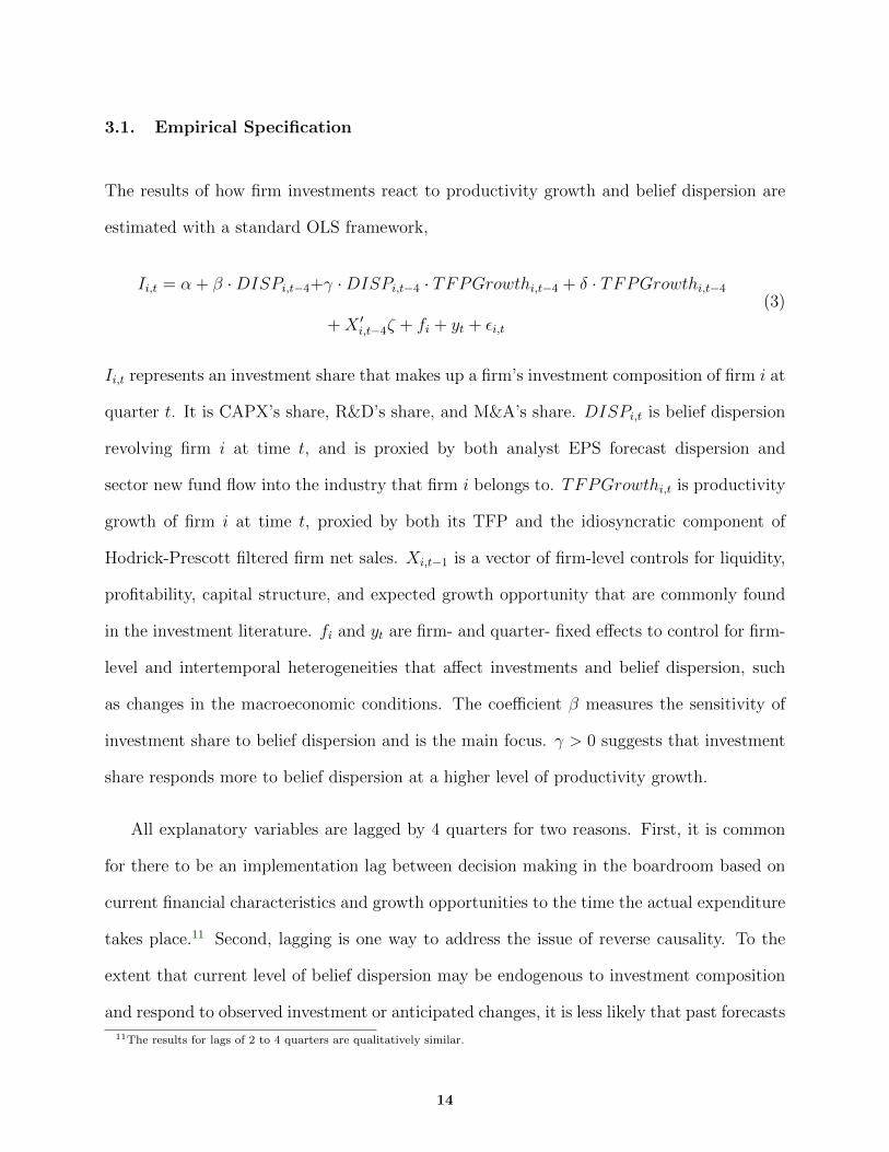
3.1. Empirical Specification

The results of how firm investments react to productivity growth and belief dispersion are

estimated with a standard OLS framework,

Ii,t = α + β ·DISPi,t−4+γ ·DISPi,t−4 · TFPGrowthi,t−4 + δ · TFPGrowthi,t−4

+X ′i,t−4ζ + fi + yt + εi,t

(3)

Ii,t represents an investment share that makes up a firm’s investment composition of firm i at

quarter t. It is CAPX’s share, R&D’s share, and M&A’s share. DISPi,t is belief dispersion

revolving firm i at time t, and is proxied by both analyst EPS forecast dispersion and

sector new fund flow into the industry that firm i belongs to. TFPGrowthi,t is productivity

growth of firm i at time t, proxied by both its TFP and the idiosyncratic component of

Hodrick-Prescott filtered firm net sales. Xi,t−1 is a vector of firm-level controls for liquidity,

profitability, capital structure, and expected growth opportunity that are commonly found

in the investment literature. fi and yt are firm- and quarter- fixed effects to control for firm-

level and intertemporal heterogeneities that affect investments and belief dispersion, such

as changes in the macroeconomic conditions. The coefficient β measures the sensitivity of

investment share to belief dispersion and is the main focus. γ > 0 suggests that investment

share responds more to belief dispersion at a higher level of productivity growth.

All explanatory variables are lagged by 4 quarters for two reasons. First, it is common

for there to be an implementation lag between decision making in the boardroom based on

current financial characteristics and growth opportunities to the time the actual expenditure

takes place.11 Second, lagging is one way to address the issue of reverse causality. To the

extent that current level of belief dispersion may be endogenous to investment composition

and respond to observed investment or anticipated changes, it is less likely that past forecasts

11The results for lags of 2 to 4 quarters are qualitatively similar.

14

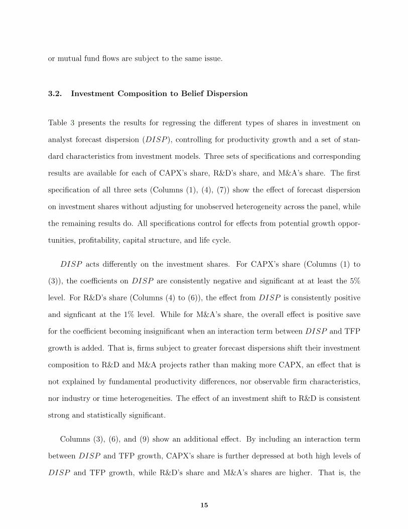
or mutual fund flows are subject to the same issue.

3.2. Investment Composition to Belief Dispersion

Table 3 presents the results for regressing the different types of shares in investment on

analyst forecast dispersion (DISP ), controlling for productivity growth and a set of stan-

dard characteristics from investment models. Three sets of specifications and corresponding

results are available for each of CAPX’s share, R&D’s share, and M&A’s share. The first

specification of all three sets (Columns (1), (4), (7)) show the effect of forecast dispersion

on investment shares without adjusting for unobserved heterogeneity across the panel, while

the remaining results do. All specifications control for effects from potential growth oppor-

tunities, profitability, capital structure, and life cycle.

DISP acts differently on the investment shares. For CAPX’s share (Columns (1) to

(3)), the coefficients on DISP are consistently negative and significant at at least the 5%

level. For R&D’s share (Columns (4) to (6)), the effect from DISP is consistently positive

and signficant at the 1% level. While for M&A’s share, the overall effect is positive save

for the coefficient becoming insignificant when an interaction term between DISP and TFP

growth is added. That is, firms subject to greater forecast dispersions shift their investment

composition to R&D and M&A projects rather than making more CAPX, an effect that is

not explained by fundamental productivity differences, nor observable firm characteristics,

nor industry or time heterogeneities. The effect of an investment shift to R&D is consistent

strong and statistically significant.

Columns (3), (6), and (9) show an additional effect. By including an interaction term

between DISP and TFP growth, CAPX’s share is further depressed at both high levels of

DISP and TFP growth, while R&D’s share and M&A’s shares are higher. That is, the

15

relationship between DISP and investment shares are reinforced when there is a higher

level of productivity growth. By itself, the coefficients on TFP growth suggest that greater

productivity growth should instead boost CAPX’s share (0.0043), which is more consistent

with intuition.

I repeat the estimation with new fund flow as a proxy for belief dispersion in Table 4. The

results are similar to that using DISP . The relationship between fund flow with CAPX’s

share and R&D’s share have the same signs and statistical significance as with DISP in

the previous table, while the relationship to M&A tends to be insignificant. However, the

additional reinforcement from high productivity growth to fund flow’s effect on investment

shares exist in this set of results, too. The coefficients on the interaction term between fund

flow and TFP growth remains statistically significant and negative for CAPX’s share, remain

positive and statistically significant for M&A’s share, and remains positive (but statistically

insignificant) for R&D’s share.

The results for the same specifications but uses idiosyncratic sales growth to proxy for

productivity growth are also estimated, but not reported. The signs of coefficients on DISP ,

the measure for productivity growth, and the interactions terms are generally consistent as

the previous tables.

The results are robust to using different measures for belief dispersion and productiv-

ity growth. They suggest firms that are subject to greater belief dispersions about their

prospects have higher investment compositions in riskier projects that are associated with

greater uncertainty and take longer resolution of outcome, such as R&D and M&A. They

also have lower relative investment in CAPX, which has less uncertainty about its expected

returns. As Coles et al. (2006) suggest, this shift in investment composition indicate a more

risky investment profile; one that is not explained by firm and industry fundamentals.

16

The evidence also suggest that not only do firms adopt a more risky investment composi-

tion when belief dispersion is high, the effect is reinforced when there is higher productivity

growth. This is not predicted by standard theories of productivity growth. The results

suggest that productivity growth affects firm investment not only through the traditional

channel, which indicate higher productivity growth raises expected return and investment

levels in physical capital should be increased. In addition, productivity growth affects firm

investment via belief dispersion. I further explore this dimension in Section 4.

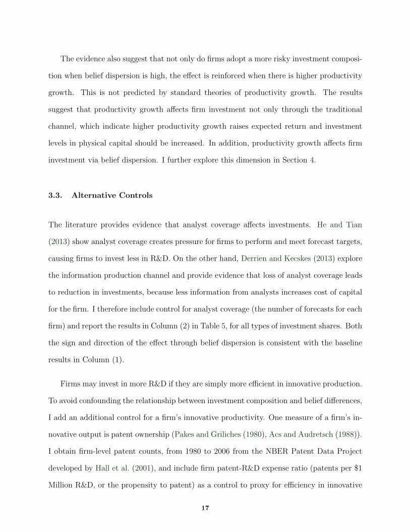
3.3. Alternative Controls

The literature provides evidence that analyst coverage affects investments. He and Tian

(2013) show analyst coverage creates pressure for firms to perform and meet forecast targets,

causing firms to invest less in R&D. On the other hand, Derrien and Kecskes (2013) explore

the information production channel and provide evidence that loss of analyst coverage leads

to reduction in investments, because less information from analysts increases cost of capital

for the firm. I therefore include control for analyst coverage (the number of forecasts for each

firm) and report the results in Column (2) in Table 5, for all types of investment shares. Both

the sign and direction of the effect through belief dispersion is consistent with the baseline

results in Column (1).

Firms may invest in more R&D if they are simply more efficient in innovative production.

To avoid confounding the relationship between investment composition and belief differences,

I add an additional control for a firm’s innovative productivity. One measure of a firm’s in-

novative output is patent ownership (Pakes and Griliches (1980), Acs and Audretsch (1988)).

I obtain firm-level patent counts, from 1980 to 2006 from the NBER Patent Data Project

developed by Hall et al. (2001), and include firm patent-R&D expense ratio (patents per $1

Million R&D, or the propensity to patent) as a control to proxy for efficiency in innovative

17

production. The results are reported in Column (3) of Table 5, for all investment shares,

show the effect of belief differences on investment composition remain robust to the inclusion

of this control.

Another important factor that affects investment allocation is CEO characteristics. The

literature of CEO tenure’s impact on investment suggests that CEOs are more likely to take

risks in the earlier periods in their tenure, when they begin to learn about the firm and are

willing to take on different initiatives to improve firm performance. As CEO tenure grows,

CEOs become entrenched and tend to prefer the status quo, e.g., Miller (1991), Berger

and Ofek (1999). The stage of CEOs life cycle appears important for decisions on firms’

investment mix. I control for the cumulative years in office of the present CEO. To do so, I

collect insider trading data from the Thompson Reuters Table One file, which records non-

derivative transactions of insiders and specifically of CEOs. I track the cumulative tenure for

each firm’s CEO since the beginning of the file. A CEO’s tenure stops when a new person

ID begins to make trades in the CEO role in lieu of the previous person ID. I estimate the

approximate time that the previous person stepped down from being a CEO and the new

person takes office to be half-way of the duration between the last trade of the previous ID

and the first trade of the new ID.

As Columns (4) in Table 5 show, CEO tenure is related positively with CAPX’s share

and negatively with R&D’s share, and is insignificant in the case of M&A’s share. The sign

is consistent with the life cycle story that as CEOs stay longer in office, they tend to avoid

more risky investments such as M&As. The effects of DISP on investment shares remain

robust as before.

To supplement the results, I also control for CEO turnover, which is an indicator variable

that takes on the value of 1 if the CEO ID changes, and zero otherwise. In the literature,

CEO turnover is considered as an event when the new management can initiate value-

18

creating investment decisions to “correct” mistakes by previous management. Weisbach

(1995), Denis and Denis (1995), and Denis et al. (1997) present evidence that associate

CEO turnovers with divesting unprofitable acquisitions, downsizing operations, or reducing

diversification. Therefore, changing investment composition to obtain a less risky profile

is expected to be associated CEO turnover. Results from Column (5) in Table 5 for all

investment shares corroborate the “reset” theory, and show CEO turnover to be associated

with less investment in the riskier projects (while the sign on CAPX’s share is negative but

statistically insignificant).

Stock market return also influences investment decisions. Higher market returns may

encourage managers to use the stock as an acquisition currency and invest in more M&A

projects, as suggested by Shleifer and Vishny (2003). I include control for excess market

return, which is stock return adjusted for the value-weighted market index. The evidence

from Column (6) in Table 5 is consistent with firms using stocks with high price appreciation

as an acquisition currency to finance acquisitions, since M&A’s share of investment is related

positively with higher stock returns, while R&D’s share is related negatively. The effect from

belief dispersion remains robust as in the baseline results.

Having adjusted for possible confounding factors as discussed above, it remains that

there may be other unobservable characteristics to the econometrician, but observed by

management that cause the change towards an investment composition that maximizes firm

performance. If this holds true, it is reasonable to expect that the change would be associated

with better future firm performance. As observed in the performance measures Table 8,

controlling for observed factors and unobserved heterogeneity across the panel that may

impact performance, firms with a higher investment composition in R&D do not have better

future performance, while they are exposed to greater firm risk.

19

3.4. Endogeneity and Instrumental Variable Analysis

The challenge of establishing a causal relationship of belief dispersion on investment com-

position is endogeneity and reverse causality. So far the results are estimated using lagged

explanatory variables, which may mitigate part of the concern if contemporaneous invest-

ment is not affected by past belief dispersion. However, investment could be persistent, so

lagged belief dispersion may be caused by lagged investment, which also explains current

investment.

In spite of the various controls I have included, it is perceivable that there remain unob-

served firm or market characteristics that determine investment decisions and belief disper-

sion jointly. It is also plausible that the direction of causality is opposite to what is supposed.

Some characteristics of the firm (unobserved by the econometrician) may dictate that the

firm should adjust its investment composition to some optimal level, such as adopting a more

risky and aggressive investment profile, thus analysts revise their expectations accordingly.

To mitigate this concern, I use merger of brokerage houses as a natural experiment

that introduces exogenous variation to the formation of forecasts and dispersion. Hong and

Kacperczyk (2010) collects a sample of thirteen brokerage mergers between 1994 and 2005

affecting 1,261 of the firms in my sample,12 and they show that the mergers resulted in a

decrease in analyst coverage because redundant analysts are let go.

The merger of two brokerages provides a reasonable identification for exogenous variation

in belief dispersion for two reasons. First, a merger considered here is likely to be an indepen-

dent event from individual firm policies or actions. As summarized in Hong and Kacperczyk

(2010), the thirteen mergers are driven by brokers expanding into different business lines

or geographic areas, or one broker is taking over another broker in trouble. Merger-related

12They identified two other mergers that are outside of my sample span.

20

termination of analysts is also unlikely to affect the forecasts of other analysts or that of

market sentiments regarding particular stocks. Other studies that use similar measures to

study the information content of forecast coverages include Kelly and Ljungqvist (2012) and

Derrien and Kecskes (2013). Second, I show that after a merger event through which analyst

coverage reduces, belief dispersion increases.

Hong and Kacperczyk (2010) find that less coverage causes analysts to make more opti-

mistic forecasts because of less competition, resulting in less accurate information production.

Kelly and Ljungqvist (2012) report that termination of analyst coverage is correlated with

increase in information asymmetry in that there is less information production. Both sets

of evidence indicate that reduction in analyst coverage should be related to greater belief

dispersion, because public signals have become more noisy. Consistent with this evidence

and theory, I first find the mergers of brokerage houses that affect the firms in my sample are

associated with reduction in analyst coverage by 1.32 analysts, an effect that is statistically

significant at the 1% level and comparable to previous work. Second, I show reduction in

coverage is associated with greater dispersion. To do so, I begin with a plot of the average

number of estimates versus forecast dispersion for different sectors over time, which is pre-

sented in Figure 1. The figure suggests that, for many of the sectors, increases in the number

of estimates, or analyst coverage, is generally accompanied by decreases in belief dispersion.

Often, the peak in the number of estimates is matched by a trough in the dispersion mea-

sure. Next, I find that increasing coverage by one analyst is associated with reducing belief

dispersion by 0.0598, statistically significant at the 1% level. The evidence is consistent with

the idea that more analyst coverage is related with less dispersion, and I will provide further

evidence in the first-stage results below.13

Specifically, I construct a dummy variable MERGER as an instrument for belief dis-

13In the limit, when the number of estimates, or analyst coverage, reaches unity, the dispersion should be zero. However, asseen in Figure 1, most industries are covered by more than 4 analysts on average.

21

persion. MERGER for a firm-quarter equals one if a brokerage merger happened and the

firm was covered by the parties involved, and equals zero otherwise. If the merger happens

at the end of the fiscal quarter for the firms, such as the case of Kidder Peabody & Co’s

merger with PaineWebber Group on December 31, 1994, I have tried a variation that assigns

MERGE to one for the quarter after, the result remains the same. Hong and Kacperczyk

(2010) also identify cases when the firm was dropped from coverage prior to the merger

date, which affected 347 firms in my sample and therefore these may not reflect exogenous

changes. I repeated the tests by dropping these observations and the results remain quali-

tatively similar. In the test, I limit the estimation sample to between 1993 and 2005 to be

within the years of the mergers. I include the same set of firm-level controls and fixed effects

as used in the baseline model.

Table 6 reports the results of the instrumental variables approach. The first column shows

the reduced form estimates of investment allocations on the instrument, MERGER, which

are significant at at least the 10% level and the estimates are of the expected signs. The

remaining columns report the first stage statistics as well as the IV estimates. For the first

stage, I regress analyst forecast dispersions on MERGER and lagged firm characteristics

that measure firm fundamentals and firm risks. Diether et al. (2002) identify that dispersion

is is positively correlated to a firm’s B/M, share turnover, trading volume, debt-to-book

ratio, earnings variability, and standard deviation of past returns, but is negatively related

to sales and size. The regression results are consistent and show that firms affected by the

merger of brokerage houses are associated with 0.0586 or 10% of standard deviation more

dispersion. The pattern is similar to the estimates in the baseline results. The measure of

belief dispersion has a positive effect on investment shares of R&D and M&A, and depresses

the CAPX’s share. The coefficients in the IV results are greater than those in the OLS

results. Since the OLS estimates contain both the causal and selection effects, the results

22

suggest that there is a negative selection effect because belief dispersion is correlated with

unobserved firm fundamental characteristics (by the econometrician) that determine firm

investment. One explanation for the negative effect can be that there is greater disagreement

or belief dispersion regarding firms with poor fundamentals.

3.5. Fractional Response Model

In any period, firms may choose to invest in any or all of physical capital, R&D, or M&A.

The investment composition in each type of project takes on the form of fractions and is

in [0, 1]. Being a bounded fractional dependent variable, the effect of explanatory variables

X may not be linear, and the variance tends to decrease when the conditional mean of

the dependent variable E(y|X) approaches its bounds. Investment shares are susceptible to

build up around either bounds, so standard OLS estimates may be biased and inconsistent.

Investment composition is not a result of censoring, so Tobit model may not be suitable.

Papke and Wooldridge (1996) address the challenge by proposing a nonlinear model for

the conditional mean of the fractional response, y, given by: E(y|X) = G(Xβ) with X

being a 1 × K vector of explanatory variables, β a K × 1 vector, and G(.) a nonlinear

function bounded between zero and one. They specify a fractional logistic link function and

estimate a consistent and asymptotically normal estimator for β using a quasi-maximum

likelihood method to maximize the Bernoulli log-likelihood function. Papke and Wooldridge

(2008) extend their earlier work for application in panel data. In this case, they use a probit

link function and obtain consistent estimates by the pooled Bernoulli quasi-MLE (QMLE)

that maximizes a pooled probit log-likelihood. To supplement the main results, I provide

alternative estimates of the specification in Equation 3 using the pooled fractional probit

estimator. Instead of having a linear specification, in the fractional model the following is

23

estimated:

E[Ii,t|DISPi,t−4, TFPGrowthi,t−4, Xi,t−4, εi,t] =

Φ(α + β ·DISPi,t−4 +X ′i,t−4ζ + εi,t)

(4)

Table 7 reports the results of this estimation. The signs of the results are consistent with

those reported in Section 3.

3.6. Investment and Performance

To gauge how investment composition is related to future firm performance, I define four

measures of firm performance with financial accounting ratios and six proxies for firm risk

as are commonly used in the literature. More specifically, the future performance and risk

measures are averages of the four-quarters forward (and repeated for eight-quarters forward).

I regress the performance measures on the investment shares, belief dispersion (using forecast

dispersion as the proxy), as well as productivity growth (TFP growth), controlling for firm-

level factors that could impact performance (such as liquidity, size, and capital structure)

and also firm- and time- fixed effects. Since the investment shares add up to one, I use

M&A’s share as the reference group and it is omitted from the estimation.

The results are summarized in Table 8. Columns (1) to (4) report the effects of analyst

forecast dispersion on performance. In general, increasing CAPX’s share is related to better

firm profitability, investment efficiency, and sales growth. Its relationship with gross margin

has a negative sign, but is insignificant. On the other hand, increasing R&D’s is associated

with worse performance across all measures.

For the risk measures, CAPX’s share is consistently related to lower risks, while increasing

R&D’s is associated with greater firm risks in the future four quarters forward. The results

24

are consistent with the literature’s stance on the relative riskiness of investment policies

through the level of investments in CAPX and R&D.

3.7. Economic Significance

Based on the identified causal effects from Table 6, a one standard deviation increase in

belief dispersion will bring about increases in R&D’s share and M&A’s share by 4.37% and

1.31%, respectively, and reduce CAPX’s share by 5.67%. To place the changes in dispersion

in perspective, there are sizable variation both cross-sectionally and across time in belief

dispersion at the firm-level (the ratio of within- over between- variations is 0.62/0.53 =

1.17).

Given Table 8, the increase in R&D’s share is thus associated with increases of 180 basis

points in cash flow volatility, 33 basis points in stock return volatility, and 78 basis points

in standard deviation in ROA, which are all averaged over the future four quarters.

4. Belief Dispersion and Corporate Investment: An Interpreta-

tion and Extension

The empirical results show belief dispersion affects firm investment allocation, and a higher

level of belief dispersion is related to relatively more investment in riskier projects, which

are related to greater firm risks. The composition effect is reinforced when a higher level of

belief dispersion is accompanied by higher productivity growth. The results are robust to

the inclusion of controls for common price-based controls such as Tobin’s Q and productivity

measure such as TFP. Taken together, the findings suggest the investment composition effect

requires an explanation when productivity and belief dispersion are considered jointly.

25

To explain the empirical results, a model can be built in the context of a market environ-

ment in which investors have resale options and there are heterogeneous beliefs and short-

sales constraints, as developed by Miller (1977), Harrison and Kreps (1978), Scheinkman and

Xiong (2003), Hong et al. (2006), and Bolton et al. (2006). In such a framework, investors

process information differently, so that firm managers-owners who have resale option in their

stakes of the firm are incentivized to invest more in riskier projects. This incentive increases

when there is productivity growth, which raises expected returns, attracts more investors,

and leads to greater expected belief dispersion.

4.1. Model

Consider a model that builds on Bolton et al. (2006) and follows similar notations. Consider

a one-period economy with three dates: d = 0, d = 1, and d = 2. There are j firms with

incumbent manager-owners. At d = 0, the manager owns 100% of the firm and makes

investment decisions. Other investors may enter the industry and buy shares of the firm at

d = 1 in the secondary market. The number of shares in the firm is normalized to one.

The firm’s investment process is as follows: the manager can choose investment by allo-

cating resources in two types of projects at d = 0 and output is realized at d = 2. Project A

produces uj, uj ∼ N(hjµj, σ2f ), in which µj is the resource allocated to operate the project or

the scale, hj > 0 measures the expected return per unit of scale, and σ2f is variance about the

return of the project that is beyond the manager’s control. Project B produces vj ≡ ωjzj, in

which ωj is the scale and zj ∼ N(0, σ2c ) is the return per unit of scale and σ2

c is the variance

on the project per unit of scale.14 In other words, scaling up investment in Project A will

increase expected long-run return without increasing the uncertainty, while project B will

increase variance of output. The firm produces total output rj = uj + vj. The remaining

14Project B is considered as the “Castle-in-the-Air” project in Bolton et al. (2006). zj has a fixed mean which is scaled tozero here. Any value of zj can be factored out and treated as a constant, so I focus on its variance-inflating aspect.

26

analysis focuses on firm j and subscript j is omitted.

At d = 1, the manager and n outside investors may trade shares in firm j on the secondary

market at d = 1 after they receive common signals about the productivity of both projects.

Each investor i is subject to a bias φi when processing the signal of Project B, that is, the

investor may overreact to the signal.15 Every investor, including the owner-manager, draws

φi i.i.d. from a publicly known, fixed and non-degenerate distribution G(.) with support

in (0,∞). Outside investors do not know φi a priori and can only make a draw after they

decide to enter the market to trade in the firm’s stock. At d = 2, the investor holding the

share in the firm receives the output and the economy ends.

Investors observe public signals s and θ about the output from projects A and B, re-

spectively. Investors update their beliefs about the firm’s output r according to the Bayes’

rule and given the manager’s optimal relative investments to the projects (µ, ω). Investors

agree on their posterior beliefs about Project A to be u = E[u|s, µ]. For Project B, however,

investors receive signal θ = z + εθ, εθ ∼ N(0, σ2θ), and differ in beliefs in the informativeness

of the signal, which is determined by their respective φi. Let τ denote the precision of a

signal, τθ = 1σ2θ. Investors, including the manager, will instead treat the precision as φiτθ,

and their subjective posteriors for Project B is given by:

vi = Ei[v|θ, ω] = λiωθ; λi ≡φiτθ

φiτθ + τz(5)

in which, φi = 1 implies the investor is not biased and φi > 1 implies the investor biases

upwards the precision of the signal, or as in Bolton et al. (2006), the investor is overconfident

about the signal.

Assuming short-sales constraints, the price of the stock at d = 1 is bid up to the highest

15A realization of φi = 1 implies the investor is not subject to the bias, whereas φi > 1 indicates the investor interprets thesignal to be more informative than it is.

27

subjective valuation of the firm (e.g., see the price-optimism models of Miller (1977), Shleifer

and Vishny (1997), etc., and empirical evidence from Diether et al. (2002), Boehme et al.

(2006)). Thus, given a set I of investors (with the manager and n outside investors), the

equilibrium price of the stock of firm j at d = 1 is the valuation of the firm is:

p1 = max{u+ vi} = u+ max∀i∈Ij{(v)i} (6)

or simply, p1 reflects the valuation of the investor who overweighs the signal θ, or analogously,

who is most optimistic.

The manager’s investment choice at d = 0 is to choose the investment scale (µ, ω) in

Projects A and B to maximize expected firm value E0[V ], given his own draw of φo and n

outside investors, and a resource constraint,

maxµj ,ωj

E0[V ]

subject to µ+ c(ω) = e

(7)

of which the resource constraint requires the total expenditure due to effort allocation into

both projects must sum up to some initial endowment e (some form of internal resources such

as the firm’s retained earnings or owner/manager’s wealth). The investment expenditure on

project A is assumed to be linear in µ, and the per unit cost is normalized to one; the

expenditure on the castle-in-the-air project is assumed to be nonlinear in ω (one can think

that such projects are subject to greater scrutiny), and is denoted by a convex function C(ω),

28

and C ′(.), C ′′(.) > 0. More precisely,

E0[V ] = E0[E(u)] + E0

[max∀i∈I{E(vi|θ, ω)}|φ0

]= hµ+ E0[max

∀i∈I{ φiτθφiτθ + τz

θω︸ ︷︷ ︸≡λiθω

}|φ0]

= hµ+ E0[max∀i∈I{λiθ}|φ0]ω

= hµ+1

2σθφ(0)

Φ(0)

E(

max∀i∈Ij{λi}|φ0

)− E

(min∀i∈Ij{λi}|φ0

)︸ ︷︷ ︸

Expected Belief Dispersion

(8)

The proof for the objective function is provided in the appendix.

4.2. Discussion

It follows from Equation 8 that the manager’s objective function contains an option com-

ponent that is increasing in the scale of variance-inflating Project B and expected investor

belief dispersion. This is also the manager’s resale option. E0[V ] is also a function of the

marginal benefits to investing in the two projects. The expected marginal return to augment

investment scale in project B for the manager is increasing in n, the number of stock market

investors. (Proved in the appendix.) When beliefs are homogeneous, the expected marginal

return to Project B is zero and no investment would be allocated to it.

As such, when the number of investors n in the marketplace increases, there is greater

expected belief dispersion. Since investors have heterogenous beliefs which bias upward their

valuations of project B, the manager optimally invest in the variance-inflating Project B to

maximize stock valuation, and in other words, the manager’s resale option value. Hence,

∂ω∂n> 0 and ∂µ

∂n< 0. In the limit, when n → ∞, this marginal benefit tends to one half the

29

inverse Mills ratio, and optimal ω is set to equate the marginal cost.

Ex-ante, investors form expectations of the firm’s output, which is a function of expected

returns on both types of projects. They will enter and participate in the market until

expected profits just offsets entry costs in the equilibrium. Intuitively, when there’s an

exogenous shock to h, which is the productivity of project A, the expected return to the firm

increases and will attract the entry of more investors. n increases.

Intuitively, if h increases, the manager should shift the investment composition to rel-

atively greater investment in project A. However, as n also increases, from the manager’s

perspective, there are two effects on the scale of project A, µ. First, the marginal return to

project A increases, so µ should be increased. Second, the option component of the man-

ager’s objective function increases with n. That is, expected belief dispersion increases and

the increasing the expected marginal benefit of Project B for the manager and ω should be

increased. If the expected marginal benefit from inflating expected belief dispersion through

ω dominates, ∂ω∂h> 0 and the investment composition is shifted to relatively more investment

in project B. In such a case, uncertainty about the firm’s output accumulates and σ(r) grows.

In Bolton et al. (2006), projects A and B are respectively referred to as “fundamental”

and “castle-in-the-air” projects, reflecting their return and risk structures. In the context of

my data and extant empirical evidence, project A can be represented by CAPX investment,

which has less uncertainty; while project B may be seen as R&D and M&A investments,

which have greater uncertainties about their expected returns.

The theoretical exercise above helps to place my results into perspective. For my first

set of results: in the presence of greater analyst forecast belief dispersion and while holding

other factors constant, the expected belief dispersion about a firm’s returns increases and

the firm maximizes firm value by changing its investment composition to favour project B’s.

30

The same holds true for when mutual fund flow in a certain sector increases, since the fund

flow is a proxy for the number of investors, an increase in n will lead to the same outcome.

Productivity growth, or a shock to h, can explain the second set of results of why a

reinforcement of the composition shift takes place. By itself, productivity growth positively

impacts CAPX’s share and generally have negative impact on R&D and M&A investments,

which is consistent with the intuition discussed previously of h’s effect on µ. At the same

time, productivity growth attracts more investors such that the option value effect dominates.

Therefore, at high levels of productivity growth and belief dispersion, there is a reinforcement

effect.

Several key assumptions drive the results. One, both heterogeneous beliefs and short-

sales constraints exist; two, the investors and owner have a resale option. The analysis also

suggests that greater information transparency will reduce excessive risk taking, because it

leads to more precise information on stochastic projects, reducing the effect from individual

bias.

Empirically, a review of the history of booms and busts shows that market investors and

sentiments have important roles in investment behaviour. As early as the tulip mania in 1637,

investors were willing to buy tulip bulbs at yet higher prices because many expected that the

bulbs can be resold at higher prices. Mackay (1848) recorded that “Nobles, citizens, farmers,

mechanics, seamen, footmen, maidservants, even chimney sweeps and old clotheswomen,

dabbled in tulips.” Later, the South Sea Company’s stock price rose by over 700% during

the 1720s through advertising to investors of its potential profitable trading strategy in South

America, while making no real investments.

Relatedly, the role of more inexperienced or individual investors in price booms is being

noted increasingly. Brennan (2004) argues the participation of first-time investors in the

31

equity markets to contribute to the technology boom in the 1990s, using aggregate U.S. data

on direct equity ownership or through mutual funds or self-directed retirement accounts.

Greenwood and Nagel (2009) find younger mutual fund managers invested heavily in tech-

nology stocks at the height of the technology boom in comparison to their more experienced

and older peers. Using data from other countries, Gong et al. (2010) attribute a continuous

inflow of new investors to be the most significant factor of price appreciation of the Baosteel

call warrants, the first derivative in China after a lengthy suspension. Kaustia and Knupfer

(2011) document new investor entry rates at five-times the average during the technology

boom, which is driven by recent gains by the investors’ peers. More recently and with a

musical twist, Kim and Jung (2013) attribute 800% increase in market capitalization for a

Korean semi-conductor firm – owned by the father of the singer of “Gangnam Style” – in

mere two months to both domestic and foreign individual investor enthusiasm about the

popular song, when there was no material new information about the firm’s fundamentals.

The idea that more investor entry to the stock market increases belief dispersion is con-

sistent with previous studies. Grinblatt and Keloharju (2001), Lamont and Thaler (2003),

and Vissing-Jorgensen (2003) provide evidence that new, unsophisticated, and overconfident

investors are more likely to enter the stock market during booms. While Barber and Odean

(2008) find that individual investors, who are limited in their ability to process informa-

tion on available stocks, tend to purchase attention-grabbing stocks. Greenwood and Nagel

(2009) document that inexperienced investors are more likely to chase the trend (for exam-

ple, loading their portfolios with technology stocks) that contribute to price appreciation.

Antoniou et al. (2012) build on the earlier results and find that asset prices to be less in

line with fundamentals during optimistic periods due to the presence of more optimistic

investors. Taken together, the evidence suggest that more investors enter the stock market

with optimistic expectations in the market during booms that are initiated by some form

32

of productivity growth, and these investors tend to flock to stocks experiencing high growth

and media exposure.

Is it possible that managers are simply at a loss with what to invest in? In my iden-

tification strategy, I conjectured and established a setting in which the loss in analysts led

to greater disagreement or belief dispersion, which I attribute to reduced information. It is

well known that analysts provide information for firm decision makers, too. The reduction

in information from the loss in analyst coverage could impact managers’ investment choices

not because they are trying to exploit disagreement, but because they themselves are not

certain which projects are best for the firm. This line of reasoning is not consistent with two

facts. First, I find a reinforcement effect of the investment composition effect when there

is productivity growth as reported earlier. In this case, the marginal return to capital has

clearly risen and it follows that more CAPX should be made relative to the other two types

of investments. Second, Derrien and Kecskes (2013) find that reduction in analyst coverage,

which increases information asymmetry and raises cost of capital, causes firms to reduce

investment levels in all projects. Therefore, firms do not appear to be investing in any ran-

dom project because they are uncertain which one to pick best as a result of losing expert

advice from analyst reduction. In sum, my results identify a different channel in which the

manager-owner changes investment composition to exploit belief dispersion.

ChapterName

5. Conclusion

This paper provides evidence that corporate investment allocation decisions are sensitive

to belief dispersion. Firms change their investment composition to include more relative

investment in riskier projects such as R&D and M&A. This relationship is robust to controls

33

for firm and industry fundamentals. The composition effect is present even when there is a

positive return shock to CAPX investment, and reinforced when greater belief dispersion is

accompanied by high return shock. To explain the empirical findings, I build a simple model

based on Bolton et al. (2006) to explain the effect that belief dispersion have on investment

composition. In a market with heterogeneous investor opinions about uncertain returns,

along with limits to arbitrage or significant short selling constraints, stock prices are bid

up to the highest subjective valuations. Investor beliefs then matter for firm investment

allocation when the manager-owner has a resale option, i.e., the manager-owner can sell firm

shares to more optimistic investors. Since investors disagree more on riskier projects and it

is more likely that someone will value riskier projects more highly when belief dispersion is

greater, the firm owner’s resale option grows in expected value as belief dispersion increases,

encouraging more investment allocation to riskier projects. Firms that are more productive

may be more incentivized to invest in riskier projects at a time of high market valuations,

because higher expected returns attract more investors, which leads to greater likelihood

of more optimistic valuations. My results then suggest a channel of how efficient capital

allocation during the boom can lead to misallocation, which can potentially explain the

phenomenon of countercyclical capital misallocation found in studies such as Eisfeldt and

Rampini (2008) and Bloom et al. (2012).

References

Acs, Z. J. and D. B. Audretsch (1988): “Innovation in Large and Small Firms: AnEmpirical Analysis,” The American Economic Review, 78, pp. 678–690.

Antoniou, C., J. A. Doukas, and A. Subrahmanyam (2012): “Sentiment, NoiseTrading, and the CAPM,” Journal of Economic Perspectives.

Baker, M., J. C. Stein, and J. Wurgler (2003): “When Does The Market Matter?Stock Prices And The Investment Of Equity-Dependent Firms,” The Quarterly Journal ofEconomics, 118, 969–1005.

Baker, M. and J. Wurgler (2011): “Behavioral Corporate Finance: An Updated Sur-vey,” Working Paper 17333, National Bureau of Economic Research.

34

Barber, B. M. and T. Odean (2008): “All That Glitters: The Effect of Attentionand News on the Buying Behavior of Individual and Institutional Investors,” Review ofFinancial Studies, 21(2), 785–818.

Barberis, N. and R. Thaler (2003): “A Survey of Behavioral Finance,” Handbook ofthe Economics of Finance, 1, 1053–1128.

Bargeron, L. L., K. M. Lehn, and C. J. Zutter (2010): “Sarbanes-Oxley and cor-porate risk-taking,” Journal of Accounting and Economics, 49, 34 – 52.

Berger, P. and E. Ofek (1999): “Causes and effects of corporate refocusing programs,”Review of Financial Studies, 12, 311–345.

Berk, J. B., R. C. Green, and V. Naik (2004): “Valuation and Return Dynamics ofNew Ventures,” Review of Financial Studies, 17, 1–35.

Bloom, N., M. Floetotto, N. Jaimovich, I. Saporta-Eksten, and S. J. Terry(2012): “Really Uncertain Business Cycles,” .

Boehme, R. D., B. R. Danielsen, and S. M. Sorescu (2006): “Short-Sale Constraints,Differences of Opinion, and Overvaluation,” Journal of Financial and Quantitative Anal-ysis, 41, 455–487.

Bolton, P., J. Scheinkman, and W. Xiong (2006): “Executive Compensation andShort-Termist Behaviour in Speculative Markets,” Review of Economic Studies, 73, 577–610.

Bond, P., A. Edmans, and I. Goldstein (2012): “The Real Effects of Financial Mar-kets,” Annual Review of Financial Economics, 4(1), 339–360.

Brennan, M. J. (2004): “How Did It Happen?” Economic Notes, 33, 3–22.

Chambers, D., R. Jennings, and I. Thompson, RobertB. (2002): “Excess Returnsto R&D-Intensive Firms,” Review of Accounting Studies, 7, 133–158.

Chatterjee, S., K. John, and A. Yan (2012): “Takeovers and Divergence of InvestorOpinion,” Review of Financial Studies, 25, 227–277.

Chen, J., H. Hong, and J. C. Stein (2002): “Breadth of ownership and stock returns,”Journal of Financial Economics, 66, 171–205.

Chen, Q., I. Goldstein, and W. Jiang (2007): “Price Informativeness and InvestmentSensitivity to Stock Price,” Review of Financial Studies, 20, 619–650.

Chirinko, R. S. and H. Schaller (1996): “Bubbles, fundamentals, and investment: Amultiple equation testing strategy,” Journal of Monetary Economics, 38, 47–76.

——— (2011): “Fundamentals, Misvaluation, and Business Investment,” Journal of Money,Credit and Banking, 43, 1423–1442.

Choy, S. K. and J. Wei (2012): “Option trading: Information or differences of opinion?”Journal of Banking & Finance, 36, 2299 – 2322.

35

Coles, J. L., N. D. Daniel, and L. Naveen (2006): “Managerial incentives and risk-taking,” Journal of Financial Economics, 79, 431 – 468.

Denis, D. J. and D. K. Denis (1995): “Performance Changes Following Top ManagementDismissals,” The Journal of Finance, 50, 1029–1057.

Denis, D. J., D. K. Denis, and A. Sarin (1997): “Agency Problems, Equity Ownership,and Corporate Diversification,” The Journal of Finance, 52, 135–160.

Derrien, F. and A. Kecskes (2013): “The Real Effects of Financial Shocks: Evidencefrom Exogenous Changes in Analyst Coverage,” The Journal of Finance, 68, 1407–1440.

Diether, K. B., C. J. Malloy, and A. Scherbina (2002): “Differences of opinion andthe cross-section of stock returns,” Journal of Finance, 57(5), 2113–2141.

Ding, D. and M. M. Rahaman (2012): “Booms, Busts, and the Market for CorporateControl,” Working Paper.

Eisfeldt, A. L. and A. A. Rampini (2008): “Managerial Incentives, Capital Realloca-tion, and the Business Cycle,” Journal of Financial Economics, 87, 177–199.

Evans, R. B. (2010): “Mutual Fund Incubation,” The Journal of Finance, 65, 1581–1611.

Gilchrist, S., C. P. Himmelberg, and G. Huberman (2005): “Do Stock Price BubblesInfluence Corporate Investment?” Journal of Monetary Economics, 52, 805–827.

Gong, B., P. Deng, and S. Dong-hui (2010): “New Investers and Bubbles: An Analysisof the Baosteel Call Warrant Bubble,” Unpublished working paper.

Greenwood, R. and S. Nagel (2009): “Inexperienced investors and bubbles,” Journalof Financial Economics, 93, 239–258.

Grinblatt, M. and M. Keloharju (2001): “What Makes Investors Trade?” The Journalof Finance, 56, 589–616.

Hall, B. H., A. B. Jaffe, and M. Trajtenberg (2001): “The NBER patent citationsdata file: Lessons, insights and methodological tools,” NBER Working Papers 8498.

Harrison, J. M. and D. M. Kreps (1978): “Speculative Investor Behavior in a StockMarket with Heterogeneous Expectations,” The Quarterly Journal of Economics, 92, 323–36.

He, J. J. and X. Tian (2013): “The dark side of analyst coverage: The case of innovation,”Journal of Financial Economics, 109, 856–878.

Hoberg, G. and G. Phillips (2010): “Real and Financial Industry Booms and Busts,”Journal of Finance, 65, 45–86.

Hobijn, B. and B. Jovanovic (2001): “The Information-Technology Revolution and theStock Market: Evidence,” American Economic Review, 91, 1203–1220.

Hong, H. and M. Kacperczyk (2010): “Competition and Bias,” The Quarterly Journalof Economics, 125, 1683–1725.

36

Hong, H., J. Scheinkman, and W. Xiong (2006): “Asset Float and Speculative Bub-bles,” The Journal of Finance, 61, 1073–1117.

Jensen, M. C. (2005): “Agency Costs of Overvalued Equity,” Financial Management, 34,5–19.

Kandel, E. and N. D. Pearson (1995): “Differential Interpretation of Public Signalsand Trade in Speculative Markets,” Journal of Political Economy, 103, 831–72.

Kaustia, M. and S. Knupfer (2011): “Peer performance and stock market entry,” Jour-nal of Financial Economics, In Press, Corrected Proof, –.

Kelly, B. and A. Ljungqvist (2012): “Testing Asymmetric-Information Asset PricingModels,” Review of Financial Studies, 25, 1366–1413.

Kim, Y. H. A. and H. S. Jung (2013): “Investor PSY-chology Surrounding ’GangnamStyle’,” Working Paper.

Kothari, S., T. Laguerre, and A. Leone (2002): “Capitalization versus Expensing:Evidence on the Uncertainty of Future Earnings from Capital Expenditures versus R&DOutlays,” Review of Accounting Studies, 7, 355–382.

Lamont, O. A. and R. H. Thaler (2003): “Can the Market Add and Subtract? Mis-pricing in Tech Stock Carve-outs,” Journal of Political Economy, 111, 227–268.

Mackay, C. (1848): Memoirs of Extraordinary Popular Delusions & the Madness ofCrowds, London: Richard Bentley, New Burlington Street, first ed.

Miller, D. (1991): “Stale in the Saddle: CEO Tenure and the Match Between Organizationand Environment,” Management Science, 37, 34–52.

Miller, E. M. (1977): “Risk, Uncertainty, and Divergence of Opinion,” The Journal ofFinance, 32, pp. 1151–1168.

Mitchell, M. L. and K. Lehn (1990): “Do Bad Bidders Become Good Targets?” Journalof Applied Corporate Finance, 3, 60–69.

Morck, R., A. Shleifer, and R. W. Vishny (1990): “The Stock Market and Invest-ment: Is the Market a Sideshow?” Brookings Papers on Economic Activity, 21, 157–216.

Olley, G. S. and A. Pakes (1996): “The Dynamics of Productivity in the Telecommu-nications Equipment Industry,” Econometrica, 64, 1263–97.

Pakes, A. and Z. Griliches (1980): “Patents and R&D at the firm level: A first report,”Economics Letters, 5, 377 – 381.

Papke, L. E. and J. M. Wooldridge (1996): “Econometric Methods for FractionalResponse Variables with an Application to 401(K) Plan Participation Rates,” Journal ofApplied Econometrics, 11, 619–32.

——— (2008): “Panel Data Methods for Fractional Response Variables with an Applicationto Test Pass Rates,” Journal of Econometrics, 145, 121–133.

37

Pastor, L. and P. Veronesi (2009): “Technological Revolutions and Stock Prices,”American Economic Review, 99, 1451–83.

Polk, C. and P. Sapienza (2009): “The Stock Market and Corporate Investment: ATest of Catering Theory,” Review of Financial Studies, 22, 187–217.

Raghavendra Rau, P. and T. Vermaelen (1998): “Glamour, Value and the Post-Acquisition Performance of Acquiring Firms,” Journal of Financial Economics, 49, 223–253.

Ramey, G. and V. A. Ramey (1995): “Cross-Country Evidence on the Link betweenVolatility and Growth,” American Economic Review, 85, 1138–51.

Sapp, T. and A. Tiwari (2004): “Does Stock Return Momentum Explain the&quot;Smart Money&quot; Effect?” Journal of Finance, 59, 2605–2622.

Scheinkman, J. A. and W. Xiong (2003): “Overconfidence and Speculative Bubbles,”Journal of Political Economy, 111, 1183–1219.

Shi, C. (2003): “On the Trade-Off between the Future Benefits and Riskiness of R&D: ABondholders’ Perspective,” Journal of Accounting and Economics, 35, 227 – 254.

Shleifer, A. and R. W. Vishny (1997): “The Limits of Arbitrage,” Journal of Finance,52, 35–55.

——— (2003): “Stock Market Driven Acquisitions,” Journal of Financial Economics, 70,295 – 311.

Shumway, T. (2001): “Forecasting Bankruptcy More Accurately: A Simple Hazard Model,”The Journal of Business, 74, 101–24.

Sirri, E. R. and P. Tufano (1998): “Costly Search and Mutual Fund Flows,” Journalof Finance, 53, 1589–1622.

Stein, J. (1989): “Effcient Capital Markets, Ineffcient Firms: A Model of Myopic CorporateBehavior,” Quaterly Journal of Economics, 104, 655–670.

Stein, J. C. (1996): “Rational Capital Budgeting in an Irrational World,” The Journal ofBusiness, 69, 429–55.

Vissing-Jorgensen, A. (2003): “Perspectives on Behavioral Finance: Does ”Irrational-ity” Disappear with Wealth? Evidence from Expectations and Actions,” NBER Macroe-conomics Annual.

Weisbach, M. S. (1995): “CEO Turnover and the Firm’s Investment Decisions,” Journalof Financial Economics, 37, 159 – 188.

Xiong, W. (2013): “Bubbles, Crises, and Heterogeneous Beliefs,” NBER Working Papers18905, National Bureau of Economic Research, Inc.

38

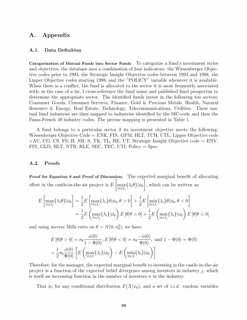
A. Appendix

A.1. Data Definition

Categorization of Mutual Funds into Sector Funds To categorize a fund’s investment stylesand objectives, the database uses a combination of four indicators: the Wiesenberger Objec-tive codes prior to 1993, the Strategic Insight Objective codes between 1993 and 1998, theLipper Objective codes starting 1998, and the ”POLICY” variable whenever it is available.When there is a conflict, the fund is allocated to the sector it is most frequently associatedwith; in the case of a tie, I cross-reference the fund name and published fund prospectus todetermine the appropriate sector. The identified funds invest in the following ten sectors:Consumer Goods, Consumer Services, Finance, Gold & Precious Metals, Health, NaturalResource & Energy, Real Estate, Technology, Telecommunications, Utilities. These mu-tual fund industries are then mapped to industries identified by the SIC-code and then theFama-French 49 industry codes. The precise mapping is presented in Table 1.

A fund belongs to a particular sector if its investment objective meets the following:Wiesenberger Objective Code = ENR, FIN, GPM, HLT, TCH, UTL; Lipper Objective code=AU, CG, CS, FS, H, NR, S, TK, TL, RE, UT; Strategic Insight Objective code = ENV,FIN, GLD, HLT, NTR, RLE, SEC, TEC, UTI; Policy = Spec.

A.2. Proofs

Proof for Equation 8 and Proof of Discussion: The expected marginal benefit of allocating

effort in the castle-in-the-air project is E

[max∀i∈Ij{λiθ}|φ0

], which can be written as:

E

[max∀i∈Ij{λiθ}|φ0

]=

1

2E

[max∀i∈Ij{λi}θ|φ0, θ > 0

]+

1

2E

[min∀i∈Ij{λi}θ|φ0, θ < 0

]=

1

2E

(max∀i∈Ij{λi}|φ0

)E [θ|θ > 0] +

1

2E

(min∀i∈Ij{λi}|φ0

)E [θ|θ < 0]

and using inverse Mills ratio on θ ∼ N(0, σ2θ), we have:

E [θ|θ > 0] = σθφ(0)

1− Φ(0), E [θ|θ < 0] = σθ

−φ(0)

Φ(0), and 1− Φ(0) = Φ(0)

=1

2σθφ(0)

Φ(0)

[E

(max∀i∈I{λi}|φ0

)− E

(min∀i∈I{λi}|φ0

)]Therefore, for the manager, the expected marginal benefit to investing in the castle-in-the-airproject is a function of the expected belief divergence among investors in industry j, whichis itself an increasing function in the number of investors n in the industry.

That is, for any conditional distribution F (X|x0), and a set of i.i.d. random variables

39

X, with X = {x1, x2, ..., xn}

P (xmax < a|x0)

= P (x1 < a|x0)P (x2 < a|x0)...P (xn < a|x0)

= F n(x < a|x0)

Hence, it follows that for any n′ > n, F n(x|x0) > F n′(x|x0), and using the property of first

order stochastic dominance, E

(max∀i∈I′{λi}|λ0

)> E

(max∀i∈I{λi}|λ0

), where set I contains n

investors and set I ′ contains n′ investors, and n′ > n. Similarly, applying the above in reverse

also follows that E

(min∀i∈I′{λi}|λ0

)< E

(min∀i∈I{λi}|λ0

), where set I contains n investors and

set I ′ contains n′ investors, and n′ > n.�

40

Table 1: Mapping of Mutual Fund Sector Codes to Fama-French 49 Industry Codes

Mutual Fund Sectors Fama-French 49 Industries

1 Gold 27 Gold, Precious Metals2 Consumer Goods 9 Consumer goods3 Consumer Services 33 Personal Services4 Financial Services 45 Banking5 Health 11 Health Care

12 Medical Equipment6 Natural Resources 30 Oil, Petroleum and Natural Gas

29 Coal28 Non-Metallic and Industrial Metal Mining

7 Technology 35 Computer Hardware36 Computer Software 37 Chips Electronic Equipment

8 Telecommunication 32 Telecommunication9 Utilities 31 Utilities10 Real Estate 47 Real Estate

41

Figure 1: Number of Estimates and Analyst Forecast Dispersion

This graph plots, for each industry sector, the evolution of the average analyst quarter-ahead EPS forecastdispersion (y-axis on the left) and number of estimates (y-axis on the right) over time.

42

Table 2: Summary Statistics

Age is the number of quarters since the first quarter this firm appears on CRSP. Firm Size is ln(TotalAssets). Leverage is long termdebt over last period’s total assets. Tobin’s Q is computed as market value of assets divided by book value of assets. ROE is computedby earnings over last period’s book equity. Cash Flow is cash flow, sum of earnings before extraordinary items and depreciation andamortization, scaled by last period’s PPE(plant, property, and equipment). Gross Margin is (net sales - cost of goods sold)/net sales.ROA is operating income before interest, taxes, depreciation, and amortization, scaled by book value of total assets. Stock Return isquarterly stock return adjusted for industry average. Asset Growth growth rate of total assets. Sales Growth growth rate of net sales.σ(Sales Growth), computed as the standard deviation of net sales growth rates for a 8-quarter forward rolling window as in Rameyand Ramey (1995). Cash Flow Volatility, computed as ln[EBITAt − EBITAt−1] as in Shumway (2001).

CAPX is the ratio of physical capital expenditure to total investment expenditure (physical capital expenditure + R&D expenditure+ M&A expenditure). R&D is the ratio of research and development expenditure to total investment expenditure (physical capitalexpenditure + R&D expenditure + M&A expenditure). M&A is the ratio of mergers and acquisition expenditure to total investmentexpenditure (physical capital expenditure + R&D expenditure + M&A expenditure).

TFP Growth is quarter-over-quarter growth in TFP, and TFP is estimated using the Olley-Pakes (1996) method and is described in thedata section in the text. Idiosyncratic Sales Growth is the idiosyncratic component of Hodrick-Prescott filtered quarter-over-quarterchange in net sales. Number of Estimates is the mean number of EPS estimates recorded in I/B/E/S for the firm every quarter. MeanEstimates is the mean EPS estimate (quarter ahead) for the firm. Estimate Dispersion (DISP) is analyst forecast standard deviationover absolute mean forecast value for the firm. Industry New Fund flow is the new fund flow to a particular sector in the period,

computed as TNA-weighted industry average of ffk,t =TNAk,t−TNAk,t−1×(1+rk,t)

TNAk,t, where TNA is total net asset in fund k in the

particular sector.

Obs Mean Std. Dev. 25th 50th 75th

Firm Characteristicslog(Age) 188653 3.71 0.79 3.14 3.85 4.34log(Firm Size) 188661 6.57 1.86 5.18 6.45 7.77Leverage 187011 0.17 0.18 0.01 0.12 0.28Tobin’s Q 188661 1.77 1.99 0.82 1.25 2.05ROE 185709 0.02 0.28 0.00 0.03 0.05Cash Flow 161563 0.10 4.35 0.04 0.10 0.25Gross Margin 188661 0.18 2.80 0.22 0.36 0.55ROA 168682 0.03 0.04 0.01 0.03 0.05Market Excess Return 185717 0.01 0.31 -0.14 -0.01 0.1Asset Growth 184509 0.03 0.13 -0.01 0.02 0.05Sales Growth 106459 0.03 0.26 -0.04 0.03 0.1σ(Sales Growth) 83048 0.16 0.19 0.06 0.11 0.19σ(Cash Flow) 152226 1.22 2.06 -0.17 1.16 2.57σ(Profitability) 188065 0.06 2.72 0.00 0.01 0.04

CEO Tenure (quarters) 114756 23.16 22.52 7.00 18.00 31.00Number of Patents 45477 25.94 60.54 1.00 4.00 16.00Patent per Million R&D Expenditure 31815 3.59 32.22 0.26 0.84 2.67

Investment RatiosCAPX 182934 0.71 0.37 0.33 1.00 1.00R&D 182934 0.23 0.34 0.00 0.00 0.50M&A 182934 0.06 0.21 0.00 0.00 0.00

ProductivityTFP Growth 95234 0.01 0.25 -0.06 0.02 0.09Idiosyncratic Sales Growth 160488 0.37 84.62 -24.69 -1.75 17.03

Analyst EPS Forecast, Quarter-aheadNumber of Estimates 188661 7.50 6.13 3.00 5.00 10.00Mean Estimates 188661 1.03 1.92 0.19 0.60 1.50Estimate Dispersion (DISP) 188661 0.24 0.41 0.04 0.08 0.20

Mutual Fund FlowIndustry New Money Flow 77628 0.18 1.50 -0.01 0.03 0.10

43

Tab

le3:

InvestmentComposition

and

BeliefDispersion

(Analyst

Fore

cast

Dispersion)

This

table

rep

ort

spanel

regre

ssio

nre

sult

sof

invest

ment

com

posi

tion

on

belief

dis

pers

ion.

The

dep

endent

vari

able

sare

invest

ment

share

sin

CA

PX

,R

&D

,and

M&

A,

resp

ecti

vely

,and

const

ructe

das

the

invest

ment

ineach

typ

eover

the

tota

lin

vest

ment

exp

endit

ure

,w

hic

his

asu

mover

these

invest

ments

.T

he

measu

refo

rb

elief

dis

pers

ion

isanaly

stE

PS

fore

cast

dis

pers

ion.

All

expla

nato

ryvari

able

sare

lagged

by

4quart

ers

.E

stim

ate

Dis

persi

on

(DIS

P)

isanaly

stfo

recast

standard

devia

tion

over

abso

lute

mean

fore

cast

valu

efo

rth

efi

rm.

TF

PG

row

this

quart

er-

over-

quart

er

gro

wth

inT

FP

,and

TF

Pis

est

imate

dusi

ng

the

Olley-P

akes

(1996)

meth

od

and

isdesc

rib

ed

inth

edata

secti

on

inth

ete

xt.

Tobin

’sQ

iscom

pute

das

mark

et

valu

eof

ass

ets

div

ided

by

book

valu

eof

ass

ets

.C

ash

Flo

wis

cash

flow

,su

mof

earn

ings

befo

reextr

aord

inary

item

sand

depre

cia

tion

and

am

ort

izati

on,

scale

dby

last

peri

od’s

PP

E(p

lant,

pro

pert

y,

and

equip

ment)

.R

OE

iscom

pute

dby

earn

ings

over

last

peri

od’s

book

equit

y.

Siz

eisln

(TotalAssets

).A

ge

islo

gof

the

num

ber

of

quart

ers

since

the

firs

tquart

er

this

firm

app

ears

on

CR

SP

.L

evera

ge

islo

ng

term

debt

over

last

peri

od’s

tota

lass

ets

.

Inth

eta

ble

,“*”

denote

ssi

gnifi

cance

at

the

10%

level;

“**”

denote

ssi

gnifi

cance

at

the

5%

level;

“***”

denote

ssi

gnifi

cance

at

the

1%

level.

The

bra

ckets

beneath

coeffi

cie

nt

est

imate

sconta

int-

stati

stic

scom

pute

dfr

om

hete

rosk

edast

icit

y-r

obust

standard

err

ors

clu

stere

dby

firm

,w

here

Nu

m.

Fir

mis

identi

fied.

Tim

efixed

eff

ects

at

the

quart

er

level,

and

firm

fixed

eff

ects

are

inclu

ded.

CA

PX

’sShare

R&

D’s

Share

M&

A’s

Share

(1)

(2)

(3)

(4)

(5)

(6)

(7)

(8)

(9)

DIS

P-0

.0218***

-0.0

037**

-0.0

034**

0.0

179***

0.0

024**

0.0

023**

0.0

039***

0.0

013***

0.0

011***

(-3.3

9)

(-2.0

9)

(-2.0

8)

(5.4

0)

(2.5

3)

(2.5

2)

(7.3

2)

(3.6

8)

(3.6

3)

DIS

P×

TF

PG

row

th-0

.0025*

0.0

017**

0.0

008**

(-1.7

4)

(2.2

8)

(2.2

0)

TF

PG

row

th0.0

165***

0.0

054**

0.0

051**

-0.0

143***

-0.0

021*

-0.0

021*

-0.0

022

-0.0

033

-0.0

030*

(3.3

2)

(2.3

0)

(2.2

6)

(-2.9

5)

(-1.7

5)

(-1.7

8)

(-0.9

6)

(-1.3

7)

(-1.8

1)

Tobin

’sQ

0.0

215***

0.0

051***

0.0

051***

-0.0

254***

-0.0

076***

-0.0

076***

0.0

039***

0.0

025***

0.0

025***

(12.2

6)

(5.8

9)

(5.8

9)

(-10.8

2)

(-7.7

4)

(-7.7

4)

(6.0

4)

(2.8

6)

(2.8

6)

Cash

Flo

w0.0

070**

0.0

005

0.0

005

-0.0

082**

-0.0

011

-0.0

011

0.0

012*

0.0

006*

0.0

006*

(2.1

4)

(1.3

9)

(1.3

8)

(-2.2

3)

(-0.2

9)

(-0.2

9)

(1.7

9)

(1.9

5)

(1.9

5)

RO

E0.0

672***

0.0

131

0.0

133

-0.0

901***

-0.0

372***

-0.0

373***

0.0

229***

0.0

241***

0.0

240***

(5.0

6)

(1.6

2)

(1.6

3)

(-5.1

2)

(-3.8

6)

(-3.8

5)

(3.5

8)

(3.4

0)

(3.3

9)

Siz

e0.0

266***

0.0

228***

0.0

228***

-0.0

215***

-0.0

051

-0.0

051

-0.0

051***

-0.0

177***

-0.0

177***

(4.7

1)

(5.5

2)

(5.5

2)

(-6.4

1)

(-1.4

7)

(-1.4

7)

(-7.0

1)

(-5.9

6)

(-5.9

6)

Age

0.0

104

0.0

099

0.0

099

0.0

064

0.0

037

0.0

037

-0.0

168***

-0.0

136**

-0.0

136**

(0.0

6)

(1.2

0)

(1.2

1)

(1.0

7)

(0.5

4)

(0.5

4)

(-3.6

8)

(-2.4

9)

(-2.4

9)

Levera

ge

0.0

459***

0.0

497***

0.0

498***

-0.0

245***

-0.0

155

-0.0

155

-0.0

214

-0.0

342***

-0.0

343***

(17.3

6)

(3.5

4)

(3.5

4)

(-18.2

7)

(-1.4

6)

(-1.4

6)

(-0.0

4)

(-6.2

2)

(-6.2

3)

Const

ant

0.6

064***

0.6

255***

0.6

255***

0.3

585***

0.1

938***

0.1

938***

0.0

351***

0.1

807***

0.1

807***

(24.5

1)

(21.4

6)

(21.4

6)

(14.8

7)

(7.9

9)

(7.9

9)

(6.1

9)

(8.0

5)

(8.0

5)

Fir

mF

EN

oY

es

Yes

No

Yes

Yes

No

Yes

Yes

Tim

eF

EN

oY

es

Yes

No

Yes

Yes

No

Yes

Yes

R2

0.1

322

0.6

966

0.6

966

0.1

627

0.8

185

0.8

185

0.0

040

0.1

172

0.1

172

Adj.R

20.6

771

0.6

771

0.8

068

0.8

068

0.0

604

0.0

604

Num

.O

bs

76064

76064

76064

76064

76064

76064

76064

76064

76064

Num

.F

irm

s4508

4508

4508

4508

4508

4508

4508

4508

4508

44

Tab

le4:

InvestmentComposition

and

BeliefDispersion

(New

Fund

Flow)

This

table

rep

ort

spanel

regre

ssio

nre

sult

sof

invest

ment

com

posi

tion

on

belief

dis

pers

ion.

The

dep

endent

vari

able

sare

invest

ment

share

sin

CA

PX

,R

&D

,and

M&

A,

resp

ecti

vely

,and

const

ructe

das

the

invest

ment

ineach

typ

eover

the

tota

lin

vest

ment

exp

endit

ure

,w

hic

his

asu

mover

these

invest

ments

.T

he

measu

refo

rb

elief

dis

pers

ion

isnew

secto

rfu

nd

flow

.

All

expla

nato

ryvari

able

sare

lagged

by

4quart

ers

.F

un

dF

low

isth

enew

fund

flow

tom

utu

al

funds

apart

icula

rse

cto

rin

the

peri

od,

com

pute

das

TN

A-w

eig

hte

din

dust

ryavera

ge

of

ffk,t

=[TNA

k,t

−TNA

k,t

−1×

(1+rk,t

)]/TNA

k,t

,w

here

TN

Ais

tota

lnet

ass

et

infu

ndk

inth

epart

icula

rse

cto

r.T

FP

Gro

wth

isquart

er-

over-

quart

er

gro

wth

inT

FP

,and

TF

Pis

est

imate

dusi

ng

the

Olley-P

akes

(1996)

meth

od

and

isdesc

rib

ed

inth

edata

secti

on

inth

ete

xt.

Tobin

’sQ

iscom

pute

das

mark

et

valu

eof

ass

ets

div

ided

by

book

valu

eof

ass

ets

.C

ash

Flo

wis

cash

flow

,su

mof

earn

ings

befo

reextr

aord

inary

item

sand

depre

cia

tion

and

am

ort

izati

on,

scale

dby

last

peri

od’s

PP

E(p

lant,

pro

pert

y,

and

equip

ment)

.R

OE

iscom

pute

dby

earn

ings

over

last

peri

od’s

book

equit

y.

Siz

eisln

(TotalAssets

).A

ge

islo

gof

the

num

ber

of

quart

ers

since

the

firs

tquart

er

this

firm

app

ears

on

CR

SP

.L

evera

ge

islo

ng

term

debt

over

last

peri

od’s

tota

lass

ets

.

Inth

eta

ble

,“*”

denote

ssi

gnifi

cance

at

the

10%

level;

“**”

denote

ssi

gnifi

cance

at

the

5%

level;

“***”

denote

ssi

gnifi

cance

at

the

1%

level.

The

bra

ckets

beneath

coeffi

cie

nt

est

imate

sconta

int-

stati

stic

scom

pute

dfr

om

hete

rosk

edast

icit

y-r

obust

standard

err

ors

clu

stere

dby

firm

,w

here

Nu

m.

Fir

mis

identi

fied.

Tim

efixed

eff

ects

at

the

quart

er

level,

and

firm

fixed

eff

ects

are

inclu

ded.

CA

PX

’sShare

R&

D’s

Share

M&

A’s

Share

(1)

(2)

(3)

(4)

(5)

(6)

(7)

(8)

(9)

Fund

Flo

w-0

.0072***

-0.0

024*

-0.0

022*

0.0

061***

0.0

019***

0.0

017**

0.0

011***

0.0

005*

0.0

005*

(-8.5

8)

(-1.9

5)

(-1.6

9)

(10.0

1)

(2.7

5)

(2.4

3)

(3.0

1)

(1.7

3)

(1.7

3)

Fund

Flo

w×

TF

PG

row

th-0

.0044**

0.0

038**

0.0

006

(-2.2

6)

(2.5

1)

(0.6

6)

TF

PG

row

th0.0

043

0.0

037

0.0

047

-0.0

028

-0.0

015

-0.0

023

-0.0

015**

-0.0

022**

-0.0

024**

(0.3

5)

(0.1

0)

(0.2

6)

(-1.5

6)

(-1.2

0)

(-1.6

2)

(2.4

4)

(-1.6

8)

(-1.6

6)

Tobin

’sQ

0.0

141***

0.0

039***

0.0

039***

-0.0

178***

-0.0

069***

-0.0

069***

0.0

037***

0.0

030***

0.0

030***

(11.4

4)

(6.2

9)

(6.2

7)

(-9.6

7)

(-4.3

0)

(-4.2

8)

(6.8

4)

(5.5

3)

(5.5

3)

Cash

Flo

w0.0

016*

0.0

020***

0.0

020***

-0.0

019*

-0.0

023***

-0.0

023***

0.0

003*

0.0

003*

0.0

003*

(1.7

4)

(2.9

4)

(2.9

5)

(-1.9

2)

(-3.0

6)

(-3.0

8)

(1.9

6)

(1.8

1)

(1.8

2)

RO

E0.1

094***

0.0

673***

0.0

672***

-0.1

153***

-0.0

759***

-0.0

758***

0.0

059

0.0

086*

0.0

086*

(2.9

1)

(2.7

0)

(2.7

0)

(-2.8

6)

(-2.6

6)

(-2.6

6)

(1.5

0)

(1.8

4)

(1.8

4)

Siz

e0.0

205***

0.0

126

0.0

126

-0.0

160***

-0.0

057***

-0.0

057***

-0.0

045***

-0.0

069***

-0.0

069***

(3.1

3)

(0.7

7)

(0.7

8)

(-5.4

0)

(-3.7

5)

(-3.7

6)

(-12.4

7)

(-12.0

5)

(-12.0

5)

Age

0.0

259***

0.0

264***

0.0

264***

-0.0

160**

-0.0

193***

-0.0

193***

-0.0

099***

-0.0

072***

-0.0

072***

(3.6

7)

(4.6

1)

(4.6

1)

(-2.3

0)

(-3.3

8)

(-3.3

8)

(-7.0

3)

(-4.5

1)

(-4.5

1)

Levera

ge

0.6

944***

0.2

015***

0.2

015***

-0.6

919***

-0.1

906***

-0.1

906***

-0.0

026

-0.0

109

-0.0

109

(26.2

5)

(8.1

8)

(8.1

8)

(-27.0

2)

(-8.8

5)

(-8.8

5)

(-0.3

6)

(-1.5

6)

(-1.5

6)

Const

ant

0.4

630***

0.7

817***

0.7

817***

0.5

001***

0.2

103***

0.2

103***

0.0

369***

0.0

081

0.0

081

(19.0

8)

(28.1

6)

(28.1

6)

(20.9

6)

(7.5

6)

(7.5

6)

(6.9

4)

(0.7

3)

(0.7

3)

Fir

mF

EN

oY

es

Yes

No

Yes

Yes

No

Yes

Yes

Tim

eF

EN

oY

es

Yes

No

Yes

Yes

No

Yes

Yes

R2

0.1

832

0.4

497

0.4

497

0.2

049

0.4

878

0.4

878

0.0

090

0.0

171

0.0

171

Num

.O

bs

65045

65045

65045

65045

65045

65045

65045

65045

65045

Num

.F

irm

s3555

3555

3555

3555

3555

3555

3555

3555

3555

45

Tab

le5:

InvestmentComposition

and

BeliefDispersion,Altern

ativeControls

This

table

rep

ort

spanel

regre

ssio

nre

sult

sof

invest

ment

com

posi

tion

on

belief

dis

pers

ion.

The

dep

endent

vari

able

sare

invest

ment

share

sin

CA

PX

,R

&D

,and

M&

A,

resp

ecti

vely

,and

const

ructe

das

the

invest

ment

ineach

typ

eover

the

tota

lin

vest

ment

exp

endit

ure

,w

hic

his

asu

mover

these

invest

ments

.A

ddit

ional

contr

ols

as

inth

ebase

line

specifi

cati

on

are

inclu

ded.

All

expla

nato

ryvari

able

sare

lagged

by

4quart

ers

.E

stim

ate

Dis

persi

on

(DIS

P)

isanaly

stfo

recast

standard

devia

tion

over

abso

lute

mean

fore

cast

valu

efo

rth

efi

rm.

TF

PG

row

this

quart

er-

over-

quart

er

gro

wth

inT

FP

,and

TF

Pis

est

imate

dusi

ng

the

Olley-P

akes

(1996)

meth

od

and

isdesc

rib

ed

inth

edata

secti

on

inth

ete

xt.

An

aly

stC

overa

ge

isth

enum

ber

of

analy

sts

pro

vid

ing

est

imate

sfo

rth

efirm

.P

ate

nts

per

Mil

lion

R&

Dis

the

rati

oof

pate

nts

over

R&

Dexp

endit

ure

.C

um

ula

tive

CE

OT

en

ure

isth

ecum

ula

tive

years

inoffi

ce

of

the

pre

sent

CE

O.

CE

OT

urn

over

isa

dum

my

that

takes

on

1if

anew

pers

on

isin

state

das

the

CE

O.

Sto

ck

Retu

rn

isth

efirm

’sexcess

stock

retu

rnover

the

valu

e-w

eig

hte

dm

ark

et

index.

Tobin

’sQ

iscom

pute

das

mark

et

valu

eof

ass

ets

div

ided

by

book

valu

eof

ass

ets

.C

ash

Flo

wis

cash

flow

,su

mof

earn

ings

befo

reextr

aord

inary

item

sand

depre

cia

tion

and

am

ort

izati

on,

scale

dby

last

peri

od’s

PP

E(p

lant,

pro

pert

y,

and

equip

ment)

.R

OE

iscom

pute

dby

earn

ings

over

last

peri

od’s

book

equit

y.

Siz

eisln

(TotalAssets

).A

ge

islo

gof

the

num

ber

of

quart

ers

since

the

firs

tquart

er

this

firm

app

ears

on

CR

SP

.L

evera

ge

islo

ng

term

debt

over

last

peri

od’s

tota

lass

ets

.

Inth

eta

ble

,“*”

denote

ssi

gnifi

cance

at

the

10%

level;

“**”

denote

ssi

gnifi

cance

at

the

5%

level;

“***”

denote

ssi

gnifi

cance

at

the

1%

level.

The

bra

ckets

beneath

coeffi

cie

nt

est

imate

sconta

int-

stati

stic

scom

pute

dfr

om

hete

rosk

edast

icit

y-r

obust

standard

err

ors

clu

stere

dby

firm

,w

here

Nu

m.

Fir

mis

identi

fied.

Tim

efixed

eff

ects

at

the

quart

er

level,

and

firm

fixed

eff

ects

are

inclu

ded.

CA

PX

’sShare

R&

D’s

Share

M&

A’s

Share

(1)

(2)

(3)

(4)

(5)

(6)

(1)

(2)

(3)

(4)

(5)

(6)

(1)

(2)

(3)

(4)

(5)

(6)

DIS

P-0

.0034**

-0.0

031***

-0.0

037**

-0.0

019*

-0.0

020*

-0.0

031***

0.0

023**

0.0

024**

0.0

021**

0.0

016*

0.0

016*

0.0

024**

0.0

011***

0.0

013**

0.0

014*

0.0

013*

0.0

019*

0.0

017**

(-2.0

8)

(-3.5

9)

(-2.2

0)

(-1.9

3)

(-1.9

5)

(-3.6

7)

(2.5

2)

(2.5

4)

(2.0

6)

(1.9

6)

(0.9

6)

(2.5

0)

(3.6

3)

(2.4

4)

(1.7

8)

(2.1

4)

(2.1

5)

(2.6

2)

DIS

P×

TF

PG

row

th-0

.0025*

-0.0

030*

-0.0

028**

-0.0

033*

-0.0

034*

-0.0

036*

0.0

017**

0.0

018**

0.0

019*

0.0

021**

0.0

023**

0.0

028*

0.0

008*

0.0

012*

0.0

009

0.0

012

0.0

012

0.0

008*

(-1.7

4)

(-1.6

9)

(-2.1

8)

(-1.8

7)

(-1.9

1)

(-1.6

7)

(2.2

8)

(2.1

2)

(1.9

6)

(2.2

0)

(2.1

7)

(1.9

5)

(2.2

0)

(1.9

4)

(1.2

7)

(1.5

8)

(1.5

7)

(1.9

1)

TF

PG

row

th0.0

051**

0.0

051**

0.0

040*

0.0

037

0.0

038

0.0

038**

-0.0

021*

-0.0

021*

-0.0

028

-0.0

008

-0.0

008

-0.0

012

-0.0

030*

-0.0

030**

-0.0

012

-0.0

029

-0.0

030

-0.0

026**

(2.2

6)

(2.1

1)

(1.8

3)

(0.8

5)

(0.8

5)

(2.1

3)

(1.7

8)

(1.7

2)

(1.3

1)

(-0.1

4)

(-0.1

3)

(1.3

8)

(-1.8

1)

(-2.2

0)

(-1.3

8)

(-0.4

5)

(-0.4

5)

(-2.0

8)

Analy

stC

overa

ge

0.0

034**

-0.0

035*

0.0

001**

(2.4

2)

(-1.6

7)

(2.1

7)

Pate

nts

per

Million

R&

D-0

.0021

0.0

037**

-0.0

016*

(-0.7

8)

(2.1

7)

(-1.6

5)

Cum

ula

tive

CE

OT

enure

0.0

004**

-0.0

005*

0.0

001

(2.3

4)

(-1.7

2)

(0.4

7)

CE

OT

urn

over

0.0

268

-0.0

172**

-0.0

096*

(0.8

3)

(-2.1

8)

(-1.7

1)

Sto

ckR

etu

rn0.0

040*

-0.0

060***

0.0

021**

(1.6

5)

(-2.9

5)

(2.1

5)

Fir

mF

EY

es

Yes

Yes

Yes

Yes

Yes

Yes

Yes

Yes

Yes

Yes

Yes

Yes

Yes

Yes

Yes

Yes

Yes

Tim

eF

EY

es

Yes

Yes

Yes

Yes

Yes

Yes

Yes

Yes

Yes

Yes

Yes

Yes

Yes

Yes

Yes

Yes

Yes

Adj.R

20.6

771

0.6

793

0.6

362

0.6

742

0.6

742

0.6

771

0.8

068

0.8

075

0.6

159

0.8

102

0.8

102

0.8

068

0.0

604

0.0

615

0.0

575

0.0

661

0.0

662

0.0

604

Num

.O

bs

76064

76064

10002

27854

27854

76064

76064

76064

10002

27854

27854

76064

76064

76064

10002

27854

27854

76064

Num

.F

irm

s4508

4508

1130

3300

3300

4508

4508

4508

1130

3300

3300

4508

4508

4508

1130

3300

3300

4508

46

Tab

le6:

Two-sta

geLeast-S

quare

s(2

SLS)Regre

ssion

with

Instru

mentforBeliefDispersion

This

table

rep

ort

sth

ere

sult

sfr

om

the

inst

rum

enta

lvari

able

(IV

)appro

ach

,in

whic

hb

elief

dis

pers

ion

(DIS

P)

isin

stru

mente

dw

ithMERGER

(merg

ers

inbro

kera

ge

house

s).

Both

reduced

form

panel

regre

ssio

nre

sult

sof

invest

ment

com

posi

tion

on

the

inst

rum

entMERGER

.T

he

dep

endent

vari

able

sare

invest

ment

share

sin

CA

PX

,R

&D

,and

M&

A,

resp

ecti

vely

,and

const

ructe

das

the

invest

ment

ineach

typ

eover

the

tota

lin

vest

ment

exp

endit

ure

,w

hic

his

asu

mover

these

invest

ments

.A

ddit

ional

contr

ols

as

inth

ebase

line

specifi

cati

on

are

inclu

ded.

All

expla

nato

ryvari

able

sare

lagged

by

4quart

ers

,in

clu

ded

by

not

show

nare

.T

FP

Gro

wth

isquart

er-

over-

quart

er

gro

wth

inT

FP

,and

TF

Pis

est

imate

dusi

ng

the

Olley-P

akes

(1996)

meth

od

and

isdesc

rib

ed

inth

edata

secti

on

inth

ete

xt.

Tobin

’sQ

iscom

pute

das

mark

et

valu

eof

ass

ets

div

ided

by

book

valu

eof

ass

ets

.C

ash

Flo

wis

cash

flow

,su

mof

earn

ings

befo

reextr

aord

inary

item

sand

depre

cia

tion

and

am

ort

izati

on,

scale

dby

last

peri

od’s

PP

E(p

lant,

pro

pert

y,

and

equip

ment)

.R

OE

iscom

pute

dby

earn

ings

over

last

peri

od’s

book

equit

y.

Siz

eisln

(TotalAssets

).A

ge

islo

gof

the

num

ber

of

quart

ers

since

the

firs

tquart

er

this

firm

app

ears

on

CR

SP

.L

evera

ge

islo

ng

term

debt

over

last

peri

od’s

tota

lass

ets

.

Inth

eta

ble

,“*”

denote

ssi

gnifi

cance

at

the

10%

level;

“**”

denote

ssi

gnifi

cance

at

the

5%

level;

“***”

denote

ssi

gnifi

cance

at

the

1%

level.

The

bra

ckets

beneath

coeffi

cie

nt

est

imate

sconta

int-

stati

stic

scom

pute

dfr

om

hete

rosk

edast

icit

y-r

obust

standard

err

ors

clu

stere

dby

firm

,w

here

Nu

m.

Fir

mis

identi

fied.

Tim

efixed

eff

ects

at

the

quart

er

level,

and

firm

fixed

eff

ects

are

inclu

ded.

Reduced

Form

Fir

stSta

ge

Second

Sta

ge

CA

PX

’sShare

R&

D’s

Share

M&

A’s

Share

DIS

PC

AP

X’s

Share

R&

D’s

Share

M&

A’s

Share

ME

RG

ER

-0.0

063*

0.0

049**

0.0

014*

0.0

586**

(-1.8

3)

(2.4

5)

(1.6

8)

(1.9

7)

DIS

P-0

.1669*

0.1

284*

0.0

385*

(-1.8

8)

(1.6

9)

(1.7

3)

Fir

mC

hara

cte

rist

ics

Yes

Yes

Yes

Yes

Yes

Yes

Yes

Fir

m&

Tim

eF

EY

es

Yes

Yes

Yes

Yes

Yes

Yes

Num

.O

bs

48750

48750

48750

48750

48750

48750

48750

R2

0.6

984

0.8

057

0.0

789

0.0

315

F-S

tati

stic

8.6

9

47

Table 7: Fractional Response Model

This table reports the results of investment composition on belief dispersion, estimated with a fractional probit model. The dependentvariables are investment shares in CAPX, R&D, and M&A, respectively, and constructed as the investment in each type over the totalinvestment expenditure, which is a sum over these investments. Additional controls as in the baseline specification are included.

In the table, “*” denotes significance at the 10% level; “**” denotes significance at the 5% level; “***” denotes significance at the 1%level. The brackets beneath coefficient estimates contain t-statistics computed from heteroskedasticity-robust standard errors clusteredby firm, where Num. Firm is identified. Time fixed effects at the quarter level, and firm fixed effects are included.

CAPX’s Share R&D’s Share M&A’s Share

(1) (2) (3) (4) (5) (6)

DISP -0.0151** -0.0148* 0.0134*** 0.0120*** 0.0017*** 0.0028***(-2.12) (-1.88) (3.19) (2.84) (4.21) (3.83)

TFP Growth 0.0073* 0.0065* -0.0059** -0.0048* -0.0014 -0.0017(1.93) (1.84) (-2.01) (-1.93) (-1.53) (-1.39)

DISP × TFP Growth -0.0013* 0.0092* -0.0079*(-1.67) (1.95) (-1.77)

Firm Characteristics Yes Yes Yes Yes Yes YesNum. Observations 78807 78807 78807 78807 78807 78807

48

Tab

le8:Perform

ance,In

vestments,and

Dispersion

This

table

rep

ort

spanel

regre

ssio

nre

sult

sof

vari

ous

futu

rep

erf

orm

ance

and

firm

risk

measu

res

on

invest

ment

com

posi

tion.

The

refe

rence

invest

ment

mix

isM

&A

’ssh

are

and

isom

itte

d.

The

dep

endent

vari

able

sare

resp

ecti

vely

:th

eavera

ge

of

Gro

ssM

arg

inof

the

four

quart

ers

forw

ard

from

tim

et,

com

pute

das

(net

sale

s-

cost

of

goods

sold

)/net

sale

s.R

OA

of

the

four

quart

ers

forw

ard

from

tim

et,

com

pute

das

the

op

era

ting

incom

eb

efo

rein

tere

st,

taxes,

depre

cia

tion,

and

am

ort

izati

on,

scale

dby

book

valu

eof

tota

lass

ets

.A

sset

Tu

rn

over

of

the

four

quart

ers

forw

ard

from

tim

et,

com

pute

das

sale

ssc

ale

dby

tota

lass

ets

.S

ale

sG

row

thof

the

four

quart

ers

forw

ard

from

tim

et,

com

pute

das

gro

wth

rate

of

net

sale

s.σ

(Cash

)is

cash

flow

vola

tility

of

four

quart

ers

forw

ard

from

tim

et,

com

pute

dasln

[EBITA

t−EBITA

t−

1]

as

inShum

way

(2001).σ

(Pro

fita

bil

ity)

isth

evola

tility

of

pro

fita

bilit

y,

whic

hfo

llow

sth

ecom

puta

tion

inH

ob

erg

and

Phillips

(2010)

by

regre

ssin

gR

OE

on

lagged

RO

Efo

rall

firm

sin

each

indust

ryand

findin

gth

est

andard

devia

tion

of

the

resi

duals

.σ

(Sto

ckR

et)

isfo

ur

quart

ers

ahead

avera

ged

standard

devia

tion

of

month

lyst

ock

retu

rn.σ

(RO

A)

isst

andard

devia

tion

of

RO

Aw

ith

afo

ur

quart

ers

ahead

rollin

gw

indow

.σ

(Sale

sGr4q)

isth

est

andard

devia

tion

of

net

sale

sgro

wth

rate

sfo

ra

4-q

uart

er

forw

ard

rollin

gw

indow

as

inR

am

ey

and

Ram

ey

(1995),

andσ

(Sale

sGr8q)

isth

e8-q

uart

er

vers

ion.

Market-

to-B

ook

ism

ark

et

valu

eof

ass

ets

tob

ook

valu

eof

ass

ets

.C

ash

Flo

wis

the

sum

of

earn

ings

befo

reextr

aord

inary

item

sand

depre

cia

tion

and

am

ort

izati

on,

scale

dby

last

peri

od’s

pro

pert

y,

pla

nt,

and

equip

ment.

RO

Eis

com

pute

dby

earn

ings

over

last

peri

od’s

book

equit

y.

Fir

mS

ize

isln

(TotalAssets

).L

evera

ge

islo

ng

term

debt

over

last

peri

od’s

tota

lass

ets

.

Inth

eta

ble

,“*”

denote

ssi

gnifi

cance

at

the

10%

level;

“**”

denote

ssi

gnifi

cance

at

the

5%

level;

“***”

denote

ssi

gnifi

cance

at

the

1%

level.

Quart

erl

yti

me

fixed

eff

ects

and

firm

fixed

eff

ects

are

inclu

ded.

The

bra

ckets

beneath

coeffi

cie

nt

est

imate

sconta

int-

stati

stic

scom

pute

dfr

om

hete

rosk

edast

icit

y-r

obust

standard

err

ors

clu

stere

dby

firm

.

Pefo

rmance

Fir

mR

isk

Gro

ssM

arg

inR

OA

Ass

et

Turn

over

Sale

sG

row

thσ

(Cash

)σ

(Pro

fita

bilit

y)

σ(S

tock

Ret)

σ(R

OA

)σ

(Sale

sGr4

q)

σ(S

ale

sGr8

q)

(1)

(2)

(3)

(4)

(5)

(6)

(7)

(8)

(9)

(10)

CA

PX

’sShare

-0.0

012

0.0

050***

0.0

134***

-0.0

759***

-0.0

218

-0.0

231***

-0.0

373

-0.1

400***

-0.0

162***

-0.0

136***

(-0.0

5)

(7.2

8)

(3.1

0)

(-20.3

7)

(-0.6

4)

(-3.0

9)

(-1.3

4)

(-4.1

7)

(-4.2

7)

(-3.6

2)

R&

D’s

Share

-0.4

888***

-0.0

211***

-0.1

100***

-0.1

048***

0.3

532***

0.0

748**

0.0

642*

0.1

523***

0.0

444***

0.0

477***

(-6.1

1)

(-13.4

7)

(-16.7

8)

(-18.9

6)

(7.0

4)

(2.4

2)

(1.8

8)

(3.1

6)

(5.6

3)

(5.9

6)

Mark

et-

to-B

ook

-0.0

134

0.0

043***

0.0

035***

0.0

113***

0.0

449***

-0.0

183*

-0.0

255***

0.0

440***

-0.0

006

0.0

007

(-0.6

9)

(10.4

1)

(3.7

7)

(14.3

8)

(7.2

2)

(-1.7

8)

(-6.0

4)

(7.9

6)

(-0.6

3)

(0.6

5)

Cash

Flo

w0.0

932***

0.0

025***

0.0

021***

-0.0

009

0.0

025

-0.0

065***

-0.0

023

-0.0

187**

-0.0

041***

-0.0

032**

(2.8

1)

(3.1

7)

(3.3

3)

(-0.8

4)

(0.7

2)

(-3.2

4)

(-0.4

2)

(-2.3

5)

(-3.2

4)

(-2.2

0)

RO

E0.1

884

0.0

709***

0.0

102

-0.0

221

-3.8

416***

1.4

325***

-0.3

074***

-0.0

630

-0.0

616***

-0.0

385***

(1.1

3)

(6.1

2)

(1.0

7)

(-1.1

4)

(-10.1

2)

(8.6

0)

(-4.3

1)

(-0.7

4)

(-4.5

5)

(-2.6

0)

Siz

e0.0

706***

0.0

026***

-0.0

192***

0.0

038***

0.8

872***

-0.0

215***

-0.1

064***

-0.1

576***

-0.0

176***

-0.0

177***

(6.0

6)

(8.9

8)

(-12.3

9)

(4.5

4)

(98.6

7)

(-2.8

6)

(-25.1

5)

(-18.7

3)

(-11.3

1)

(-11.1

4)

Levera

ge

-0.0

768

-0.0

089***

-0.1

757***

0.0

097

-0.4

294***

0.2

334

0.2

167***

-0.5

050***

-0.0

133

-0.0

111

(-0.9

3)

(-4.7

0)

(-12.7

0)

(1.5

1)

(-5.5

0)

(1.2

9)

(5.0

8)

(-6.8

4)

(-0.8

7)

(-0.7

2)

Const

ant

0.0

230

0.0

043

0.3

222***

0.0

681***

-3.6

388***

0.2

357***

-1.9

994***

-3.0

979***

0.9

871***

0.9

540***

(0.2

0)

(0.4

1)

(15.9

5)

(3.1

0)

(-14.6

6)

(2.5

9)

(-14.5

0)

(-8.5

4)

(3.7

4)

(3.7

2)

Tim

eF

EY

es

Yes

Yes

Yes

Yes

Yes

Yes

Yes

Yes

Yes

Indust

ryF

EY

es

Yes

Yes

Yes

Yes

Yes

Yes

Yes

Yes

Yes

R2

0.0

626

0.2

915

0.4

615

0.0

416

0.5

993

0.1

056

0.1

427

0.1

292

0.1

655

0.1

879

Num

.O

bs

82103

82103

82103

71655

52916

53133

47758

47494

74484

61459

Num

.F

irm

s4254

4254

4254

4103

3592

3601

3373

3469

4103

3254

49