Behaviour of Multi-Layered Laminated Glass Under Blast Loading

by

Michelle Parratt

A thesis submitted in conformity with the requirements for the degree of Master of Applied Science in Civil Engineering

Department of Civil Engineering

University of Toronto

© Copyright by Michelle Parratt 2016

ii

Behaviour of Multi-Layered Laminated Glass Under Blast Loading

Michelle Parratt

Master of Applied Science

Department of Civil Engineering

University of Toronto

2016

Abstract This thesis outlines a three-phase research program that was developed to determine the

accuracy and applicability of various software packages in predicting the behaviour of multi-

layered laminated glass windows under blast loading. Experimental data was collected through

the completion of full-scale field blast tests. Two unique window compositions were examined

at two different scaled distances, with a total of eight specimens being tested. Small-scale

laboratory testing followed on beams of the same composition to investigate the behaviour of

multi-layered laminated glass and to derive a static resistance function for the layup. Finally, the

windows were modelled using predictive software, and the outputs of these programs were

compared to the field-collected data.

iii

Acknowledgements This thesis was not an individual effort, and I would like to take the opportunity to thank those

people who supported and helped me along the way.

First, I would like to thank my supervisor, Professor Jeffrey Packer, as well as Professor

Michael Seica, for their support and guidance over the past two years. As the path was not

always clear and the project complex, their encouragement and suggestions were central to the

completion of this project.

There were many others whose contributions made this project possible. Thanks to Exsel

Dytecna, who helped fabricate the field targets and offered their shop floor for a few days. I also

wish to thank both the staff of DNV-GL at the Spadeadam Testing and Research Centre, as well

as the staff of the University of Toronto Structural Testing Facility, without whose expertise my

testing program would not have occurred. Additionally, thanks go to Professor David

Yankelevsky of Technion Israel Institute of Technology for his involvement in this project.

I am also very grateful for the substantial financial and in-kind support provided by the Explora

Foundation towards this project and the University of Toronto’s Centre for Resilience of Critical

Infrastructure. Financial support was also received from the Ontario Graduate Scholarship fund,

the Lyon Sachs Graduate Research Fund, and the Queen Elizabeth II Graduate Scholarship in

Science & Technology fund.

Finally, a big thank you to my family and friends, whose love and support often goes without

recognition, but for which I am eternally grateful.

iv

Table of Contents Abstract ........................................................................................................................................ ii Acknowledgements ..................................................................................................................... iii List of Tables ............................................................................................................................... vi List of Figures ............................................................................................................................ vii List of Symbols ............................................................................................................................. x

1 Research Significance and Goals ........................................................................................ 1

2 Background .......................................................................................................................... 3 2.1 Blast Fundamentals .................................................................................................................. 3

2.1.1 Explosions .............................................................................................................................. 3 2.1.2 Blast Load Parameters ............................................................................................................ 4

2.2 Annealed Glass .......................................................................................................................... 8 2.2.1 Manufacture of Float Glass .................................................................................................... 8 2.2.2 Physical Structure of Glass ..................................................................................................... 9 2.2.3 Mechanical Properties .......................................................................................................... 10 2.2.4 Strength of Glass .................................................................................................................. 10 2.2.5 Strain Rate Effects on Mechanical Properties ...................................................................... 12

2.3 Strengthening of Glass............................................................................................................ 13 2.3.1 Manufacture of Thermally-Tempered Glass ........................................................................ 14 2.3.2 Behaviour of Thermally-Tempered Glass ............................................................................ 15

2.4 Laminated Glass ..................................................................................................................... 16 2.4.1 Interlayer Properties ............................................................................................................. 16 2.4.2 Polycarbonate ....................................................................................................................... 19 2.4.3 Manufacture of Laminated Glass ......................................................................................... 19 2.4.4 Behaviour of Laminated Glass ............................................................................................. 20 2.4.5 Failure Criteria ..................................................................................................................... 22

2.5 Multi-Layered Laminated Glass ........................................................................................... 23 2.5.1 Behaviour of Multi-Layered Laminated Glass ..................................................................... 23

2.6 Blast Effects on Glazing ......................................................................................................... 25 2.6.1 Response of Glazing to Blast Loads ..................................................................................... 25 2.6.2 Blast-Resistant Glazing Design ............................................................................................ 26 2.6.3 Testing Methods for Glazing Subjected to Blast Loads ....................................................... 26

2.7 Modelling ................................................................................................................................. 28 2.7.1 Plate Theory ......................................................................................................................... 29 2.7.2 Single-Degree-of-Freedom Modelling ................................................................................. 30 2.7.3 Finite Element Method ......................................................................................................... 31

2.8 Software Packages .................................................................................................................. 32 2.8.1 SBEDS.................................................................................................................................. 32 2.8.2 WINGARD ........................................................................................................................... 34 2.8.3 CWBlast ............................................................................................................................... 35

3 Field Blast Testing ............................................................................................................. 37 3.1 Targets and Reaction Structure ............................................................................................ 37 3.2 Testing Methodology .............................................................................................................. 39 3.3 Instrumentation ...................................................................................................................... 41 3.4 Initial Observations ................................................................................................................ 43 3.5 Data Processing ....................................................................................................................... 46 3.6 Blast Waves ............................................................................................................................. 46 3.7 Displacement-Time Histories ................................................................................................. 49

v

3.8 Strain Rate ............................................................................................................................... 51 3.9 Limitations and Sources of Error .......................................................................................... 52 3.10 Discussion ................................................................................................................................ 52

4 Laboratory Testing Program ........................................................................................... 53 4.1 Description of Specimens ....................................................................................................... 53 4.2 Testing Methodology .............................................................................................................. 54 4.3 Old-Composition Beams......................................................................................................... 56 4.4 New-Composition Beams ....................................................................................................... 58 4.5 Composite Behaviour ............................................................................................................. 60 4.6 Resistance Functions .............................................................................................................. 64 4.7 Limitations and Sources of Error .......................................................................................... 67 4.8 Discussion ................................................................................................................................ 68

5 Software Models................................................................................................................. 70 5.1 Modelling Methodologies ....................................................................................................... 70

5.1.1 SBEDS Modelling ................................................................................................................ 70 5.1.2 WINGARD Modelling ......................................................................................................... 71 5.1.3 CWBlast Modelling .............................................................................................................. 73

5.2 Comparison of Model Output to Experimental Data .......................................................... 74 5.2.1 SBEDS.................................................................................................................................. 74 5.2.2 WINGARD ........................................................................................................................... 79 5.2.3 CWBlast ............................................................................................................................... 84

5.3 Limitations and Sources of Error .......................................................................................... 85 5.4 Discussion ................................................................................................................................ 85

6 Conclusions and Recommendations ................................................................................. 87

7 References ........................................................................................................................... 89

Appendices ................................................................................................................................. 97

A. Field Blast Test Data ......................................................................................................... 97

B. Laboratory Test Data ...................................................................................................... 111 B.1 Example Calculations for Old-Composition Beam .................................................................. 111 B.2 Example Calculations for Resistance Function Conversion .................................................... 115 B.3 Laboratory Test Data ................................................................................................................. 118

C. Software Programs .......................................................................................................... 126 C.1 SBEDS Monolithic Resistance Function Conversion............................................................... 126 C.2 WINGARD Inputs ...................................................................................................................... 128

vi

List of Tables Table 2.1 Values of Ψ for laminated beams under different boundary and loading conditions .. 24 Table 2.2 GSA performance conditions for window system response ........................................ 28 Table 3.1 Multi-layered laminated glass window compositions ................................................. 37 Table 3.2 Test details ................................................................................................................... 39 Table 3.3 Blast wave peak positive pressure and impulse values ............................................... 47 Table 3.4 Pressure and impulse comparison to UFC-3-340-02 ................................................... 49 Table 3.5 Initial tensile strain rate values .................................................................................... 51 Table 4.1 Old-composition beam test results .............................................................................. 56 Table 4.2 New-composition beam test results ............................................................................. 59 Table 4.3 Beam behaviour compared to limits using moment of inertia .................................... 62 Table 4.4 Deflection-based effective thickness values ................................................................ 63 Table 4.5 Shear modulus comparison with data from Brackin, 2010 ......................................... 63 Table 4.6 Conversion method for old-composition layup – simply supported ........................... 66 Table 4.7 Temperature and load duration comparison ................................................................ 67 Table 4.8 Shear modulus values based on temperature and load duration .................................. 67 Table 5.1 Annealed glass material properties .............................................................................. 72 Table 5.2 Polycarbonate material properties ............................................................................... 72 Table 5.3 PVB material properties .............................................................................................. 73 Table 5.4 Analyses completed in WINGARD for each specimen .............................................. 73 Table 5.5 Analysis completed in CWBlast for each specimen .................................................... 74 Table 5.6 Case 1 SBEDS important values – Test 1 ................................................................... 76 Table 5.7 Test 1 comparison with WINGARD outputs .............................................................. 81 Table 5.8 Test 2 comparison with WINGARD outputs .............................................................. 83 Table A.1 Friedlander fit values .................................................................................................. 97 Table B.1 Average old-composition beam geometric parameters............................................. 111 Table B.2 Average new-composition beam geometric parameters ........................................... 114

vii

List of Figures Figure 2.1 Design chart relating Z to key blast parameters ........................................................... 5 Figure 2.2 Typical pressure-time history for fixed point in space ................................................. 6 Figure 2.3 Formation of Mach front from an air burst .................................................................. 8 Figure 2.4 DIF vs. strain rate for annealed glass in tension ........................................................ 13 Figure 2.5 Typical tempered glass stress distribution ................................................................. 15 Figure 2.6 Polyvinyl butyral dynamic stress-strain curve ........................................................... 17 Figure 2.7 Ionoplast stress-strain curve for low strain rates ........................................................ 18 Figure 2.8 Post-crack behaviour of laminated glass .................................................................... 22 Figure 2.9 GSA TS01 test cubicle ............................................................................................... 28 Figure 2.10 CWBlast support condition options ......................................................................... 36 Figure 3.1 Specimen naming convention – outside view ............................................................ 38 Figure 3.2 Side view of reaction structure with glass targets installed ....................................... 40 Figure 3.3 Front view of reaction structure with targets installed ............................................... 40 Figure 3.4 Test arena setup – Test 1 ............................................................................................ 41 Figure 3.5 Displacement gauge mount ........................................................................................ 42 Figure 3.6 Test 2 target instrumentation, from interior of window ............................................. 43 Figure 3.7 O-T1-S2 and O-T1-S1 ................................................................................................ 44 Figure 3.8 Test 2 old composition and new composition, from interior of window ................... 45 Figure 3.9 Raw vs. processed strain data for specimen N-T2-S2-H ........................................... 46 Figure 3.10 Pressure data filtering process - Test 1 .................................................................... 48 Figure 3.11 Reflected pressure and impulse – Test 1 .................................................................. 48 Figure 3.12 Measured central displacement – O-T1-S2 .............................................................. 50 Figure 3.13 Measured central displacement – O-T2-S1 .............................................................. 50 Figure 4.1 Old-composition cross-section ................................................................................... 53 Figure 4.2 New-composition cross-section ................................................................................. 53 Figure 4.3 Test setup schematic .................................................................................................. 54 Figure 4.4 Complete test setup .................................................................................................... 55 Figure 4.5 Old-composition force-displacement curve ............................................................... 56 Figure 4.6 Beam O6 after cracking.............................................................................................. 57 Figure 4.7 Beam O6 crack order.................................................................................................. 57 Figure 4.8 New-composition force-displacement curve .............................................................. 59 Figure 4.9 Beam N1 crack order and propagation ....................................................................... 60 Figure 4.10 Beam N1 layer slip ................................................................................................... 60 Figure 4.11 Beam O5 pre-crack strain data ................................................................................. 62 Figure 4.12 Average force-displacement curves ......................................................................... 64 Figure 4.13 Old-composition beam average resistance function development ........................... 64 Figure 4.14 SBEDS input into metal plate template to determine resistance function – simply-

supported.............................................................................................................................. 65 Figure 4.15 Converted resistance function for old-composition beams ...................................... 66 Figure 5.1 SBEDS general SDOF inputs – extended monolithic resistance function – simply

supported.............................................................................................................................. 71 Figure 5.2 SBEDS resistance functions – simply supported ....................................................... 71 Figure 5.3 CWBlast linear equivalent pressure-time history – Test 1 ......................................... 74 Figure 5.4 Case 1 SBEDS comparison – Test 1 .......................................................................... 76 Figure 5.5 Case 1 stiffness modifications – Test 1 ...................................................................... 76 Figure 5.6 Case 1 SBEDS comparison – Test 2 .......................................................................... 77 Figure 5.7 Case 1 stiffness modifications - Test 2....................................................................... 78

viii

Figure 5.8 Case 2 SBEDS comparison – Test 1 .......................................................................... 79 Figure 5.9 Lab RF fit with test 1 data .......................................................................................... 79 Figure 5.10 Test 1 comparison with WINGARD outputs ........................................................... 81 Figure 5.11 Young's modulus sensitivity study in WINGARD .................................................. 82 Figure 5.12 Test 2 comparison with WINGARD outputs ........................................................... 82 Figure 5.13 WINGARD old-composition resistance functions ................................................... 84 Figure 5.14 Test 1 comparison with CWBlast outputs ................................................................ 85 Figure A.1 Free-field pressure and impulse readings - Test 1 ..................................................... 97 Figure A.2 Reflected pressure and impulse readings - Test 1 ..................................................... 97 Figure A.3 Free-field pressure and impulse readings - Test 2 ..................................................... 98 Figure A.4 Reflected pressure and impulse readings - Test 2 ..................................................... 98 Figure A.5 Pane central displacement: O-T1-S2 ......................................................................... 99 Figure A.6 Pane central displacement: O-T2-S1 ......................................................................... 99 Figure A.7 Period of oscillation: O-T1-S2 ................................................................................ 100 Figure A.8 Period of oscillation: O-T2-S1 ................................................................................ 100 Figure A.9 Pane central strain: O-T1-S1-H ............................................................................... 101 Figure A.10 Pane central strain: O-T1-S1-V ............................................................................. 101 Figure A.11 Pane central strain: O-T1-S2-H ............................................................................. 102 Figure A.12 Pane central strain: O-T1-S2-V ............................................................................. 102 Figure A.13 Pane central strain: N-T1-S1-H ............................................................................. 103 Figure A.14 Pane central strain: N-T1-S1-V ............................................................................. 103 Figure A.15 Pane central strain: N-T1-S2-H ............................................................................. 104 Figure A.16 Pane central strain: N-T1-S2-V ............................................................................. 104 Figure A.17 Pane central strain: O-T2-S1-H ............................................................................. 105 Figure A.18 Pane central strain: O-T2-S1-V ............................................................................. 105 Figure A.19 Pane central strain: O-T2-S2-H ............................................................................. 106 Figure A.20 Pane central strain: O-T2-S2-V ............................................................................. 106 Figure A.21 Pane central strain: N-T2-S1-H ............................................................................. 107 Figure A.22 Pane central strain: N-T2-S1-V ............................................................................. 107 Figure A.23 Pane central strain: N-T2-S2-H ............................................................................. 108 Figure A.24 Pane central strain: N-T2-S2-V ............................................................................. 108 Figure A.25 Test specimen drawing - DYNA-01 ...................................................................... 109 Figure A.26 Test specimen drawing - DYNA-02 ...................................................................... 110 Figure B.1 Old-composition average cross-section ................................................................... 111 Figure B.2 Old-composition beam resistance function ............................................................. 115 Figure B.3 SBEDS metal plate input - simply-supported.......................................................... 116 Figure B.4 Beam O1 force-displacement curve ........................................................................ 118 Figure B.5 Beam O2 force-displacement curve ........................................................................ 118 Figure B.6 Beam O3 force-displacement curve ........................................................................ 119 Figure B.7 Beam O4 force-displacement curve ........................................................................ 119 Figure B.8 Beam O5 force-displacement curve ........................................................................ 120 Figure B.9 Beam O6 force-displacement curve ........................................................................ 120 Figure B.10 Beam N1 force-displacement curve ...................................................................... 121 Figure B.11 Beam N2 force-displacement curve ...................................................................... 121 Figure B.12 Beam N3 force-displacement curve ...................................................................... 122 Figure B.13 Beam N4 force-displacement curve ...................................................................... 122 Figure B.14 Beam N5 force-displacement curve ...................................................................... 123 Figure B.15 Beam O1 strain data .............................................................................................. 123 Figure B.16 Beam O5 strain data .............................................................................................. 124

ix

Figure B.17 Beam O6 strain data .............................................................................................. 124 Figure B.18 Beam N1 strain data .............................................................................................. 125 Figure C.1 SBEDS metal plate input - simply-supported.......................................................... 126 Figure C.2 Glass material property inputs for WINGARD ....................................................... 128 Figure C.3 Polycarbonate material property inputs for WINGARD ......................................... 128 Figure C.4 Interlayer material property inputs for WINGARD ................................................ 128 Figure C.5 Glass layup input in WINGARD, for Butacite interlayer ....................................... 128 Figure C.6 Window system input for WINGARD, for Butacite interlayer ............................... 129

x

List of Symbols ∆ Deflection

𝜀̇ Strain rate

γ Specific surface energy

µ Poisson’s ratio

Ψ Parameter that takes loading and boundary conditions into account (EET method)

σ Nominal stress

σc Critical stress

a Depth of flaw, distance between loading point and adjacent support

Ai Cross-sectional area of the ith layer

ANFO Ammonium nitrate fuel oil

ARA Applied Research Associates

b Waveform parameter, width of glass beam

CaO Lime

CWBlast Curtain Wall Blast

di Distance between centroid of ith layer and centroid of entire composite

DA Department of the Army

DAQ Data acquisition

DIF Dynamic increase factor

DoD Department of Defense

E Young’s modulus

Eg Young’s modulus of glass

Epc Young’s modulus of polycarbonate

EET Enhanced effective thickness

FEM Finite element method

FF Free-field pressure

F(t) Applied load

fu Ultimate static strength at failure

fud Ultimate dynamic strength at failure

G Shear modulus

Gavg Average shear modulus

heff Deflection effective thickness from I = bh3/12

xi

Hi Distance between the centroids of the ith and i+1th layers

hi Thickness of the ith glass layer

hw Deflection-based effective thickness from EET method

I Impulse, Moment of inertia

Ii Moment of inertia of the ith layer

Ir Positive impulse of reflected overpressure

Is Positive impulse of incident overpressure

Is- Negative impulse of incident overpressure

IL Layered moment of inertia

IM Monolithic moment of inertia

IR Measured moment of inertia

k Stiffness

K1 Stress intensity factor for first mode of crack opening

KC Critical stress intensity factor

KL Load factor

KLM Load-mass factor

KM Mass factor

LVDT Linear variable differential transformer

L Span length

Lw Length of shock wave

m Mass

n Parameter expressing level of composite behaviour

Na2O Soda

P Pressure, Force

P/∆ Beam stiffness

Pr Peak positive reflected pressure

Ps(t) Overpressure as a function of time

Pso Peak positive incident pressure

Pso- Peak negative incident pressure

PVB Polyvinyl butyral

R Standoff distance

RF Resistance function

RP Reflected pressure

xii

SBEDS Single-Degree-of-Freedom Blast Effects Design Spreadsheet

SDOF Single degree of freedom

SGP SentryGlas®Plus

SHPB Split Hopkinson pressure bar

SiO2 Silicon dioxide, silica

SLS Soda-lime-silica

SS Simply supported

T Period of vibration

ta Time of blast wave arrival

td Idealized positive phase load duration

ti Thickness of the ith interlayer layer

t0 Positive phase duration

TM Tension membrane

TML Tokyo Sokki Kenkyujo Co.

TNT Trinitrotoluene

TPU Polyurethane

U Shock wave velocity

UFC Unified Facilities Criteria

UFC-H Unified Facilities Criteria hemispherical charge

UFC-S Unified Facilities Criteria spherical charge

W Charge weight

WINGARD WINdow Glazing Analysis Response and Design

Y Calibration factor for stress intensity

y Displacement

ÿ Acceleration

Z Scaled distance

1

1 Research Significance and Goals

Traditionally, civilian infrastructure has been designed without considering the effects of

blast loading. This approach has been changing due to recent events worldwide, and the public’s

perceived level of danger from intentional attacks has increased. Building façades, composed

primarily of glass, represent a significant design challenge when considering blast loads due to

the brittle nature of monolithic glass. Failure of monolithic glazing elements results in the

majority of injuries in blast events, due to flying glass and the blast wave’s propagation into the

protected space, which can cause further structural damage to internal building elements. Thus,

laminated glass windows, composed of alternating layers of glass and interlayer, are used in

applications where air-blast loading is a concern. When the glass lites crack, the shards remain

bonded to the interlayer, preventing the formation of dangerous glass projectiles. In addition, the

interlayer acts as a ductile membrane post-cracking, which prevents the blast wave from

propagating into the protected space. Furthermore, multi-layered laminated glass windows (i.e.

more than two layers of glass and other materials) are used when both ballistic and blast

protection is required. While studies have been conducted on the behaviour of monolithic and

single-layer laminated glass under blast loading, there is limited available research on the

behaviour of multi-layered laminated glass.

Additionally, in order to accurately analyze and design blast-resistant glazing systems,

designers require tools that predict the behaviour of these systems under blast loading. Various

software packages exist for this purpose. However, these programs are complex to develop and

require rigorous validation. They must be able to accurately predict the blast load and determine

the dynamic response of the system to these loads. Different programs employ different methods

with varying assumptions, and thus, with similar inputs, different outputs are obtained. Thus, it

is crucial to determine which program, and associated analysis method, is best suited for

different blast-resistant glazing applications. Recent work (Spiller et al., 2016) has examined the

validity of such software when applied to monolithic glass, however no such studies have been

completed for multi-layered laminated glass windows. Without validation, it is impossible to

know which program, and which method, is best suited for the analysis and design of multi-

layered laminated glass windows.

The current research aims to fill this gap by investigating the behaviour of multi-layered

laminated glass under blast loading and determining the applicability and accuracy of available

software packages in the analysis of multi-layered laminated glass windows under blast. In order

2

to do so, full-scale blast arena tests were conducted on multi-layered laminated glass windows

which provided experimental data. In addition, beams comprised of the same materials and

layup were tested in the laboratory under four-point bending, in order to examine the behaviour

of multi-layered laminated glass beams and determine a static resistance function for the layup.

Finally, the window system was modelled using various software packages, and the predicted

response was compared to the measured response from the field tests. Ultimately, having a

better understanding of both the behaviour of multi-layered laminated glass windows and the

accuracy of software programs in their design will allow designers to better implement blast-

resistant glazing systems into their designs.

3

2 Background

2.1 Blast Fundamentals Blast loads are complex in nature, and engineers must understand their behaviour before

being able to accurately predict the effect these loads will have on a structure. This section

briefly outlines how blast loads are formed and how they can be quantified. UFC 3-340-02

“Structures to resist the effects of accidental explosions” (DoD, 2008), a comprehensive design

manual developed by the U.S. Military, is a good resource for additional information.

2.1.1 Explosions In simple terms, an explosion is a release of energy that occurs at such a high speed that

there is a local accumulation of energy at the location of the explosion. During an explosion, this

energy is dissipated through several means such as blast waves, thermal radiation, and fragment

propulsion (USACE, 2008). There are three main types of explosions: physical, nuclear, and

chemical. Physical explosions occur when there is a sudden release of mechanical energy, such

as the bursting of a pressure vessel. Nuclear explosions are created by uncontrolled high-speed

fission or fusion reactions. Chemical explosions occur due to the rapid oxidation of carbon and

hydrogen atoms (Cormie et al., 2009). This research deals solely with chemical explosions.

The rate of compound decomposition in a chemical explosion differs depending on the

quantity and chemistry of the reactants. There are two classifications for these oxidation

reactions: detonation and deflagration. A detonation is a supersonic combustion reaction. During

a detonation, an exothermic front is propelled through the explosive material, which drives a

shock front to propagate in the surrounding air. A deflagration is a subsonic combustion

reaction. In a deflagration, the explosion is propelled forward by heat from the exothermic

reaction, which heats the adjacent unreacted explosive material and ignites it. As the majority of

the chemical energy is released as heat, a shock front does not form, although there is still a

notable pressure increase during a deflagration. While the overpressure created by a deflagration

is small compared to the overpressure from a detonation, the pulse duration is longer, and thus a

similar impulse can be achieved. Compounds that detonate are referred to as high explosives

while compounds that deflagrate are called low explosives (Cormie et al., 2009). The effect of

detonations is the focus herein.

As previously mentioned, the chemistry of an explosive influences how it combusts, and

thus different explosives will produce different explosions. Therefore, a method to compare the

4

effects of different explosives is required. Using trinitrotoluene (TNT) as the basis of

comparison, all other explosive charges are converted into an equivalent mass of TNT based on

the explosive effects created. An equivalency factor greater than unity indicates the explosive

delivers more blast energy per unit mass than TNT does. There is no standard approach to

calculating this equivalency factor between an explosive and TNT. One possibility is to compare

the specific energy of the explosive. Another method uses two conversion factors, one for

pressure and one for impulse, which allows a designer to match the delivered pressure and

impulse separately (Cormie et al., 2009).

2.1.2 Blast Load Parameters The local accumulation of energy created by an explosion may be dissipated through

several mechanisms, but the topic of this thesis deals with shock waves propagated through air.

After a detonation occurs, a shock wave expands outward from the location of ground-zero into

the surrounding air. The shock wave is essentially a volume of hot, dense, high-pressure gas. As

this volume travels further from the centre of ignition, it decays in strength, decreases in

velocity, and increases in duration, which is caused primarily by spherical divergence. There is a

finite amount of energy released from the detonation, and as the volume of the shock wave

increases, it follows that the pressure must decrease (DoD, 2008). Thus, the location of a

structure relative to the site of an explosion is an important parameter in determining the blast

load on that structure. This distance is known as standoff and when combined with the quantity

of the explosive, it is used to calculate a quantity called scaled distance.

Scaled distance relates blast waves from one explosion to another. Theoretically, two

explosions with equal scaled distances will exert the same blast load on a structure. Simply put,

a large explosion far from the structure can produce the same effect as a small explosion closer

to the structure, provided they have the same scaled distance. The most widely accepted method

for determining scaled distance is Hopkinson-Cranz scaling, commonly called “cube-root”

scaling (Cormie et al., 2009). Hopkinson-Cranz scaling states that:

𝑍 = 𝑅

𝑊13⁄ (2.1)

where R is the standoff distance between the centre of the explosion and the point of interest

(i.e. the structure) in metres, W is the mass of the explosive in kilograms, and Z is the scaled

distance. Design charts, using imperial units for Z (i.e. feet and pounds), can be found in UFC 3-

5

340-02. An example of such a chart, colloquially called a spaghetti graph, is shown in Figure

2.1.

Figure 2.1 Design chart relating Z to key blast parameters (adapted from USACE 2008)

These charts have numerous curves that relate Z to key blast parameters including: peak

reflected pressure (Pr), peak incident pressure (Pso), positive phase impulse generated by the

reflected pressure (Ir), positive phase impulse generated by the incident pressure (Is), the arrival

time of the shock wave (ta), the duration of the positive phase (t0), the shock wave velocity (U),

and the length of the shock wave (Lw).

Using the above parameters, a typical pressure-time history can be plotted for a fixed point

in space experiencing a blast wave in free air, as shown in Figure 2.2. When the explosive

detonates, the pressure at the fixed point remains at ambient levels (Po). The shock wave must

travel between the detonation point and the point of interest, and the time it takes to do so is ta.

The arrival of the blast wave is characterized by a sudden increase in pressure up to the peak

incident pressure, Pso. The pressure quickly decays back to ambient as the shock wave passes

by. The duration of this positive phase is quantified by t0. Then a partial vacuum is formed,

initiating the negative phase, which reaches a peak negative pressure, Pso-. This suction occurs

because the air particles over-expand due to their momentum. As equilibrium is restored, the

blast effects are complete. Both the positive phase (Is) and negative phase (Is-) impulses can be

6

calculated by integrating the area under the pressure-time curve. Impulse is the “energy” carried

by the blast wave.

Figure 2.2 Typical pressure-time history for fixed point in space

Several models have been developed to quantify the curve in Figure 2.2. Baker (1973)

reviewed the available models and concluded that the best compromise between accuracy and

simplicity came from the modified Friedlander equation. The modified Friedlander equation

models the positive phase of the shock wave as follows:

𝑃𝑠(𝑡) = 𝑃𝑠𝑜 [1 − (𝑡 − 𝑡𝑎

𝑡0)] 𝑒−𝑏(𝑡−𝑡𝑎

𝑡0) (2.2)

where Ps(t) is the shock wave overpressure as a function of time, Pso is the peak positive incident

pressure, t is the time from detonation, ta is the arrival time, t0 is the positive phase duration, and

b is a waveform parameter. This model is only valid for the positive phase of the shock wave.

Often the negative phase of the shock wave is ignored in analysis, as it generally has little effect

on the peak response of a structure. The negative phase is not as well understood as the positive

phase, but models do exist (USACE, 2008).

The magnitude of the peak incident pressure will be significantly amplified when the shock

front interacts with a structure, or any medium denser than air. Essentially, the shock waves

7

reflect on the structure, and energy is transferred between the two. This creates a local area of

further compression, and thus the pressure local to the structure increases further. This reflected

pressure, Pr, is greater than the incident pressure that would occur in the same location. Peak

positive reflected pressure and the corresponding impulse are the two key parameters in

determining the response of a structure to a blast load. It is common to approximate this portion

of the pressure-time history into a line with a constant rate of pressure decay for simplicity. This

approximate curve has the same peak positive pressure and impulse values, and a new

parameter, td, the phase duration for the idealized curve, is introduced, which is shorter than the

actual phase duration, ta. Due to the difference in duration, the structural response is slightly

different, however this difference typically has minimal effect on the structural response and

thus is of little concern. In addition, the angle of incidence is another important parameter when

describing a blast load, because it affects the degree of pressure amplification during reflection.

A blast wave travelling perpendicular (0q) to a structure’s surface will fully reflect, whereas a

wave travelling parallel (90q) will not reflect at all (Cormie et al., 2009).

The geometry of a structure influences the effect that a blast wave has. A dynamic

discontinuity exists along the edges of the reflecting surface due to the difference between the

reflected pressure acting on the building surface and the free-field pressure acting immediately

adjacent to the structure. This causes a phenomenon called clearing, where, through wave

propagation towards the centre of the reflecting surface from all the edges, the reflected pressure

is reduced. The shorter the clearing distance, the faster the reflected overpressure dissipates,

which in turn decreases the impulse delivered to the structure by the blast wave (USACE, 2008).

The geometry and location of the charge relative to the ground also affect the blast wave.

There are three types of unconfined explosions: free air bursts, air bursts, and surface bursts. A

free air burst occurs well above any structure, and thus its shock wave is uninterrupted until it

reaches a structure on the ground. This means that the shock wave from a free air burst is not

amplified prior to reaching the structure. An air burst, also known as a spherical burst, occurs

just above the ground and to the side of the structure, as illustrated in Figure 2.3. The shock

waves will move away from the centre until they interact and reflect off the ground. Both the

incident and reflected shock waves move towards the target. The reflected wave moves through

air densified by the incident wave, which allows it to travel faster and eventually catch up with

the incident wave. The waves merge to form a Mach front, and the front includes the energy

from both waves. The point at which the incident wave, the reflected wave, and the Mach front

8

meet is called the triple point. The height of the triple point increases as the wave moves away

from the detonation site. Provided that the triple point is located higher than the height of the

structure, the structure will see a uniform load equal to that formed by a surface burst (USACE,

2008).

Figure 2.3 Formation of Mach front from an air burst

Finally, surface bursts, or hemispherical bursts, occur when the explosive is on or near ground

level. The waves immediately reflect on the ground surface and produce an amplified shock

wave 1.8 times stronger than a free air burst of the same explosive charge. Some of the energy is

dissipated through cratering and ground shock. If the ground surface was a perfect reflector, the

amplification factor would be 2.0 (Cormie et al., 2009). There are different design charts (see

Figure 2.1 for reference) for spherical and hemispherical bursts.

2.2 Annealed Glass Annealed glass is the most common type of glazing material, and its use can be

architectural or structural. This section outlines how annealed float glass is manufactured, and

the physical and mechanical properties that influence its unique behaviour when loaded.

2.2.1 Manufacture of Float Glass The float process for manufacturing glass was developed by Alistair Pilkington in the 1950s

and it has become the most common manufacturing method for flat glass. In brief, a continuous

flow of glass from a furnace is fed onto a surface of molten metal, generally tin. The flat surface

of the molten tin gives the glass a smooth finish as it cools. Once the glass cools sufficiently, it

becomes rigid and can be handled by rollers (Amstock, 1997).

9

First, the raw materials are batched and mixed. The mixture is then taken to the furnace,

where cullet is added. Cullet is clean, ground, scrap glass which is used to reduce the cost of the

mixture. The mixture is then heated to approximately 1500qC to produce molten glass, which

exits the furnace at a temperature of around 1000qC. Here, the molten glass enters a tin bath that

is approximately 6 meters wide with 50 to 75 mm of tin in the bottom. The glass is less dense

than the tin, and it spreads out on top of the colder tin surface, settling under its own self weight.

This creates two flat surfaces. As the glass moves through the tin bath, it cools and is eventually

pulled onto rollers into the annealing lehr. Annealing is a cooling process in which the rate of

cooling is controlled in order to minimize internal stresses in the glass, which are caused by high

temperature differentials in the material. The glass is cooled uniformly from 600qC to around

280qC, and then it leaves the lehr, where it is exposed to ambient temperatures. The glass is

inspected for defects using a xenon lamp, and defective sections are removed. Finally, the glass

is cut into sections and stored for future use (Amstock, 1997).

2.2.2 Physical Structure of Glass In broad terms, glass can be defined as “an inorganic product of fusion which has been

cooled to a rigid condition without crystallizing” (Scholze, 1991). Silica, or silicon dioxide

(SiO2), is the main component of most glass types, and it is sourced mainly from quartz

granules, or sand. Different proportions of silica produce different types of glass, and various

modifiers, normally metallic oxides, can be added to achieve the desired properties. The most

common type of glass is soda-lime-silica (SLS) glass, which generally consists of 70% SiO2,

15% soda (Na2O), and 10% lime (CaO), with the remaining 5% made up of other trace

materials. The addition of soda lowers the softening point, while the addition of lime improves

chemical resistance. SLS glass is used for plate and sheet glass, containers, and light bulbs. Two

other popular types of glass, borosilicate and aluminosilicate, are used in applications that

require high heat resistance, such as cookware, thermometers, and laboratory glassware

(Amstock, 1997).

In silica, each silicon atom is bonded to four oxygen atoms, and each oxygen atom is shared

between two silicon atoms, creating a tetrahedron shape, where the angle between each silicon

and oxygen atom is fixed. Pure SiO2 glass, reserved for specialized applications, has an

extremely high softening point. It is also far too viscous, with a viscosity around 1012 poises, for

drawing and blowing purposes. Thus, modifiers such as soda and lime are added, which lower

the viscosity and softening point to more manageable levels. The metallic ions fill the voids in

10

the open silica structure, and each ion removes one of the bonds between the oxygen and silicon

atoms. The new bonds are non-directional, and the overall structure is less stiff (Amstock,

1997).

As previously mentioned, glass does not crystallize. Instead, it undergoes a type of freezing

that occurs when the molten glass cools to ambient temperatures. Normally, as a liquid is

cooled, its volume decreases due to thermal contraction, as well as configurational contraction.

Configurational contraction is contraction due to structural rearrangement of the liquid. Once

the freezing point is reached, the material crystallizes, and there is a sudden decrease in volume.

The crystalline material continues to shrink due to thermal contraction after crystallization, but

at a slower rate. In glass, this process is different. The manufacturing process of glass causes it

to skip the crystallization step and supercool instead. In glass, the volume decreases due to

thermal and configurational contraction until the transformation temperature is reached. The

glass becomes so viscous (around 1013 poises) that configurational changes can no longer keep

pace with the decrease in temperature, and it ceases to undergo molecular rearrangement

appropriate to its temperature. After the transformation point, the glass continues to shrink, at a

slower rate, due to thermal contraction. At room temperature, glass has a viscosity of 1020

poises, and it acts as an elastic solid, although it is technically a liquid (Amstock, 1997).

2.2.3 Mechanical Properties Although glass can be manufactured from different materials and modifiers, the common

properties of glass are due to its glassy state and do not differ greatly between different glass

products. Glass behaves linearly elastic up until failure, where it fails in a brittle manner. Glass

has a modulus of elasticity around 70 GPa, a Poisson’s ratio of about 0.22, and a density around

2,500 kg/m3. When heated, glass will become less viscous and lose stiffness (Scholze, 1991).

2.2.4 Strength of Glass Due to the non-crystalline structure of glass, paired with its high viscosity, it is unable to

adjust its atomic structure and therefore cannot deform plastically (Khorasani, 2004). Instead,

glass deforms elastically until it instantaneously fails by fracture. Glass can be characterized by

the following strength traits: (1) failure is almost always due to tensile stress; (2) its compressive

strength is up to ten times higher than its tensile strength; (3) the ultimate strengths of identical

specimens exhibit a large amount of scatter; (4) fracture of glass almost always begins on the

surface; (5) flaws on the surface greatly decrease the strength; (6) the average strength is

11

decreased when a larger area is loaded; and (7) loading rate and environment affect strength

(Menčík, 1992). The theoretical tensile strength of plate glass, based on the bonds between

atoms, is between 1 and 100 GPa. However, windows generally fail when the internal stresses

are less than 100 MPa, up to 1,000 times lower. This discrepancy is mainly due to the presence

of microscopic flaws, invisible to the human eye, on the surface of the glass (Scholze, 1991).

Fracture mechanics can be used to explain the phenomenon behind these flaws and their

growth, which causes eventual failure. Griffith (1921) was the first to use these principles, and

he stated that surface flaws act as stress concentrators when load is applied to a flat plate of

glass. If the stresses in a crack tip are able to overcome the cohesive strength of the material, the

atoms will separate and the crack will grow. Since glass is brittle, the crack will propagate

through the material and failure will occur (Menčík, 1992). Griffith (1921) showed that strain

energy is stored in the system when a body with a crack is loaded. When a crack grows, some of

this strain energy is released. Based on an energy balance criterion, a crack will only grow if the

energy released in doing so is greater than the energy consumed in forming a new fracture

surface. Griffith defined the required stress, or critical stress, that will bring about crack growth

as:

𝜎𝑐 = √2𝐸𝛾𝜋𝑎

(2.3)

where σc is the critical stress, E is the Young’s modulus, γ is the specific surface energy, and a is

the depth of the flaw (Griffith, 1921). Only one flaw, often called the Griffith or critical flaw, is

required to cause member failure.

Later, Irwin (1957) introduced the stress intensity factor defined as:

𝐾𝐼 = 𝜎𝑌√𝜋𝑎 (2.4)

where KI is the stress intensity factor for the first mode of crack opening, σ is the nominal stress

at a given point, and Y is a calibration factor that relates to the crack shape. Mode I, called

opening, is the most applicable mode to glass, and it occurs when a tensile stress is applied

normal to the plane of the crack. There are two other loading modes, II and III, which occur

when in-plane shear and out-of-plane shear are applied to the crack. Each mode has their own

Kn formulation (Menčík, 1992). Based on Irwin’s (1957) crack growth criterion, the crack will

propagate and instantaneous failure will occur if the stress intensity factor reaches a critical

12

value, KC. KC can be determined experimentally and is called fracture toughness. For SLS glass,

KIC is between 0.72 and 0.82 MPa m1/2 (Menčík, 1992).

While exceeding σc or KC will result in instantaneous failure, crack propagation can still

occur at lower stress values. At values less than critical, cracks can grow very slowly, at

velocities in the order of millimeters per hour. This process is call sub-critical crack growth and

it is of importance when dealing with long-duration loading. At very low stress intensity levels,

the fatigue limit, KSCC, may be reached. At this point, subcritical crack growth ceases entirely

(Menčík, 1992).

2.2.5 Strain Rate Effects on Mechanical Properties It is well known that the mechanical properties of many materials are influenced by strain

rate (Nicholas, 1980). The effect that strain rate has on a material is quantified by a term called

the dynamic increase factor (DIF):

𝐷𝐼𝐹 = 𝑓𝑢𝑑

𝑓𝑢 (2.5)

where fud is the ultimate dynamic strength at failure, and fu is the ultimate static strength at

failure. Generally, the DIF of glass in compression is measured using a Split Hopkinson

Pressure Bar (SHPB) test, developed by Kolsky (1949). In a SHPB test, specimens are cut into

circular discs of uniform thickness and placed between two long bars, with the longitudinal axis

of the specimen parallel to the longitudinal axis of the bar. A compressive pulse, generated by

the striker bar, accelerates down the incident bar, through the specimen, and into the

transmission bar. The bars remain elastic, while the sample goes inelastic, often reaching its

failure stress. By measuring the one-dimensional wave propagation and strain in the two bars,

the stress-strain relationship of the specimen can be determined (Nicholas, 1980). The DIF in

tension may be measured using a Brazilian test, which is simply a modified SHPB test. Rather

than being parallel, the longitudinal axis of the specimen is perpendicular to the longitudinal

axis of the bar. Otherwise, the test is carried out in the same manner (Krynski, 2008). The SHPB

can be used to record stress-strain curves at strain rates from approximately 10 s-1 to 104 s-1.

The compressive strength of glass is generally unaffected by the strain rate. Holmquist et al.

(1995) used a SHPB to test glass in compression at 1x10-3 s-1 and 250 s-1 and found that there

was little change to the strength or Young’s modulus due to testing speed. Peroni et al. (2011)

did similar tests at 5x10-4 s-1 and 103 s-1 and received similar results. However, Zhang et al.

13

(2012) found that the compressive strength increased dramatically at strain rates higher than 100

s-1, achieving DIFs between 2.0 and 3.0. The authors cited differences in glass composition

between the studies as a potential source of discrepancy.

The tensile strength of glass, however, always exhibits a DIF greater than 1.0 when the

strain rate is increased. Krynski (2008) performed Brazilian tests using the SHPB at a strain rate

of 10 s-1 and calculated a DIF of 1.6. Peroni et al. (2011) conducted similar tests and found a

DIF of approximately 1.55 for a strain rate of 1000 s-1. Zhang et al. (2012) did 30 Brazilian tests

with strain rates up to 1000 s-1 and developed the following empirical relationship between

annealed glass tensile DIFs and strain rates:

𝐷𝐼𝐹 = 1.137 + 0.015 log(𝜀)̇ 𝑤ℎ𝑒𝑛 1.0−5 ≤ 𝜀̇ ≤ 350 (2.6)

𝐷𝐼𝐹 = −2.911 + 1.608 log(𝜀)̇ 𝑤ℎ𝑒𝑛 350 ≤ 𝜀̇ (2.7)

where 𝜀̇ is the strain rate. Here, the DIF increases gradually up to a strain rate of 350 s-1, after

which the strength increases quickly, as shown in Figure 2.4.

Figure 2.4 DIF vs. strain rate for annealed glass in tension (adapted from Zhang et al. (2012))

2.3 Strengthening of Glass It is common practice to strengthen annealed glass when additional bending resistance is

required. This can be achieved either by removing surface flaws or by prestressing the glass

through a process called tempering. Surface flaws can be removed by etching or applying a

chemical solution to the surface. Both options produce a flawless surface, however the condition

is short-lived, and new flaws readily form due to post processing and use (Scholze, 1991). Thus,

removing surface flaws is not an effective way to increase the bending resistance in the long

14

term. Tempering is achieved through either a thermal or chemical process. The thermal process

utilizes high temperatures to heat the annealed glass to a plastic state. Then, the glass is cooled

rapidly, leaving the inner core in tension and the outer surfaces in compression (Cormie et al.,

2009). Chemical tempering is primarily done by submersing the glass in a molten salt bath,

lower in temperature than the annealing point of the glass (Amstock, 1997). The main

mechanism in chemical tempering is ion exchange, which results in the surface glass having

either a lower coefficient of expansion or an intrinsically higher specific volume than the core

glass. This puts the surface into pre-compression. (Gardon, 1985). In both thermally- and

chemically-tempered glass, the pre-compression in the outer surfaces must be overcome before

tensile stresses can develop in the extreme fibres and crack initiation can occur (Cormie et al.,

2009). This research utilizes thermally-tempered glass, which is hence discussed further.

2.3.1 Manufacture of Thermally-Tempered Glass Thermally- or air-tempered glass is produced by heating an annealed-glass pane to

approximately 650qC via an air blast, where it reaches a plastic state. The pane then is cooled at

a controlled rate using cold air, which puts the surface into compression and the core into

tension. The resulting stress distribution can be seen in Figure 2.5. It can be manufactured in one

of two ways. The annealed glass is either hung vertically from clips along its top edge or placed

horizontally on steel rollers, which is specified by ASTM C1048, “Standard Specification for

Heat-Strengthened and Fully Tempered Glass” (2012). In both cases, the glass moves through

four basic zones: (1) a loading zone, (2) a heating zone, (3) a tempering or quenching zone, and

(4) an unloading zone. The horizontal method is preferred as the processing time is reduced and

there are no clip marks along the top edge (Amstock, 1997). All fabrication work that is

required, such as cutting to overall dimensions, drilling holes, and smoothing edges, must be

completed before the tempering process occurs. Once the glass has been tempered, it cannot be

modified without causing fracture of the entire pane (ASTM, 2012a).

15

Figure 2.5 Typical tempered glass stress distribution (adapted from Khorasani 2004)

Two types of glass can be manufactured from this process, namely heat-strengthened glass

and tempered glass. Heat-strengthened glass is heated to a lower temperature and is cooled at a

slower rate than tempered glass, and thus it has a lower level of pre-compression (Amstock,

1997). According to ASTM C1048, heat-strengthened glass must have a surface compression

between 24 and 52 MPa, whereas tempered glass must have a minimum surface compression of

69 MPa and a minimum edge compression of 67 MPa. Surface and edge compression values can

be determined through light refraction methods using a polarimeter (ASTM, 2012a).

2.3.2 Behaviour of Thermally-Tempered Glass Thermally-tempered glass exhibits higher bending resistance than annealed glass. Its

fracture behaviour is also different. Heat-strengthened glass is approximately two times as

strong as annealed glass in bending. The fracture pattern depends on the magnitude of the

surface compression. At the lower range, between 24 MPa and 31 MPa, it fractures into angular

shards, much like annealed glass, but the fragments are larger and thus fewer in number, usually

without sharp points. In the middle range, between 31 MPa and 48 MPa, the crack pattern

becomes smaller with more fragments. At surface compression values above 48 MPa, it

becomes increasingly difficult to differentiate between heat-strengthened and tempered glass

based on fragment size alone. The middle range is ideal for most applications, as the crack

pattern is large and the fragments tend to jam together, remaining in the frame (Amstock, 1997).

Tempered glass is four to five times stronger than annealed glass in bending. Due to the

high amount of pre-compression in tempered glass, failure results in the formation of small,

blunt-edged cubes commonly referred to as dice. While blunt, these fragments can act as

projectiles because, unlike heat-strengthened glass, the glass fragments do not tend to lock

16

together and thus do not stay in place. This behaviour is not ideal for blast applications (Cormie

et al., 2009).

All other physical and mechanical properties remain unchanged by the tempering process.

This includes compressive strength, hardness, specific gravity, coefficient of expansion,

softening point, thermal conductivity, solar transmittance, and stiffness. It should be noted that

since the stiffness is not altered, glass that has been thermally tempered will exhibit the same

deflection behaviour as annealed glass under the same load, provided it is of the same size and

thickness (Amstock, 1997).

2.4 Laminated Glass Although monolithic glass panes are appropriate for most building applications, there exist

situations where the enhanced strength and behaviour of laminated glass are required.

Laminated glass is composed of alternating layers of glass and interlayer (Cormie et al., 2009).

There is no restriction on the combination of glass plies used, and thus laminated glass can be

manufactured from lites of equal or unequal thicknesses, as well as the same or different heat

treatments. This allows glass composites to be designed specifically for their intended purpose

(Amstock, 1997).

2.4.1 Interlayer Properties Different interlayer materials can be used depending on the performance criteria of the

laminated glass pane. The most common interlayer material is polyvinyl butyral (PVB), which

is soft and very ductile. It is produced by mixing polyvinyl alcohol with butyraldehyde, and it is

sold under trade names such as Saflex® and Butacite®. PVB is favoured for its optical clarity

and mechanical properties. It is classified as a viscoelastic material, and as such its mechanical

properties are influenced by strain rate, level of strain, and temperature (Vallabhan et al., 1992).

In this research, strain rate is a key characteristic, as blast loading typically produce strain rates

in structural elements between 102 and 104 s-1, according to Ngo et al. (2007). Both small-strain

and large-strain behaviours are also important when dealing with laminated glass, as the PVB

interlayer experiences small strains during the pre-crack phase and large strains during the post-

crack phase. Temperature is another key variable as most laminated glass panes are used as

windows, which can be exposed to varying service temperatures. Thus, understanding the effect

that these three properties have on the behaviour of PVB is vital.

17

Since PVB is the most common interlayer material, many researchers have studied its

behaviour under a variety of loading and atmospheric conditions. Bennison et al. (1999) and

Van Duser et al. (1999) have shown that the shear modulus of PVB exposed to small strains at

low strain rates can be expressed through a generalized Maxwell series. In dynamic testing at

small strains, it has been shown that PVB behaves with either a glassy modulus in the order of 1

GPa or a rubbery modulus in the order of 1 MPa (Hooper et al., 2012a). Rubbery behaviour

occurs at lower strain rates or higher temperatures. Glassy behaviour occurs at higher strain

rates or lower temperatures. The transition temperature is between 5 and 40qC, which

corresponds to typical service temperatures for windows (Du Bois et al., 2003).

The large strain behaviour has also been examined in both quasi-static and dynamic regimes.

Researchers have found that PVB displays viscoelastic properties in the quasi-static regime, and

loading speed influences the behaviour. In the dynamic regime, PVB behaves differently,

resembling an elasto-plastic material. There is a steep initial rise in stress, followed by a pseudo

yielding point where the rate of increase vastly decreases, as shown in Figure 2.6 (Zhang et al.,

2015a). However, this is not a sign of yielding, as the extension is recoverable when the load is

removed (Hooper et al., 2012a). After this pseudo yielding point, the behaviour is either

viscoelastic exponential or viscoelastic linear, depending on the strain rate. Traditionally, an

elasto-plastic model with strain hardening has been used to quantify this behaviour, however,

recent research has shown that a bilinear viscoelastic model is more appropriate when the

unloading phase is considered. The pseudo yielding point increases with strain rate. In addition,

as the strain rate increases, PVB becomes increasingly brittle, causing it to fail at lower strain

values (Zhang et al., 2015a).

Figure 2.6 Polyvinyl butyral dynamic stress-strain curve (adapted from Zhang et al., 2015a)

18

Another interlayer, called ionoplast, is beginning to replace PVB in laminated glass

windows where residual load-carrying capacity after breakage is required, such as in blast and

impact loading. Ionoplast is composed of ethylene and methacrylic acid copolymers, as well as

metal salts, which enhance bonding between it and the glass plies (Zhang et al., 2015c).

Ionoplast is sold under the brand name SentryGlas®Plus (SGP). SGP is five times stronger

against tearing and a hundred times more rigid than PVB. As such, the overall thickness of a

laminated lite can be reduced and deflections are reduced compared to windows manufactured

using PVB (Patterson, 2011). Like PVB, its behaviour is dependent on strain rate. In general,

SGP exhibits elasto-plastic behaviour under uniaxial tension. When exposed to a low strain rate,

the stress increases sharply before it reaches yield, which is its peak stress value. The stress then

drops and the SGP continues to elongate significantly, without much appreciable increase in

stress. This behaviour is shown in Figure 2.7. As the strain rate increases, there are numerous

changes in the behaviour of SGP. Most notably, the sharp drop after yield disappears and the

SGP starts to exhibit glassy behaviour. In addition, the failure strain decreases, the yield stress

increases, and the material becomes less ductile. Unlike PVB, not all the deformation is

recoverable, but as the strain rate increases, the amount of recoverable deformation increases as

well (Zhang et al., 2015c).

Figure 2.7 Ionoplast stress-strain curve for low strain rates

Aliphatic thermoplastic polyurethane (TPU) can also be used as an interlayer in laminated

glass. It is created by reacting diisocyanate with a linear polyether or polyester polyol and a diol

or amine chain extender and is produced as a sheet material (Folgar, 2005). TPU has similar

strength and ductility properties to PVB, but it remains ductile at sub-zero service temperatures

19

and maintains its stiffness at high temperatures. TPU is more expensive than PVB, which limits

its use to specialized applications, such as ballistic-resistant glazing (Cormie et al., 2009). In

ballistic-resistant glazing, TPU, instead of PVB, is used to adhere a polycarbonate sheet (see

Section 2.4.2 Polycarbonate) to a sandwich of PVB-laminated glass. TPU bonds much better to

polycarbonate, which helps reduce the likelihood of delamination (Folgar, 2005). TPU is also

designed to accommodate the large difference in thermal expansion coefficients between glass

and polycarbonate. Finally, TPU is preferred over PVB as plasticizers contained in PVB can

react with the polycarbonate, causing it to cloud up and limit light transmission through the

laminate (Ykman, 1991).

Poured acrylic resin is another type of interlayer. However, its usefulness is limited as it

does not exhibit the same membrane behaviour as those interlayers previously mentioned.

Laminates made with resin have little advantage over monolithic glass panes when used

structurally (Cormie et al., 2009). Resin is generally used to enhance acoustic performance

(Ledbetter et al., 2006). This research uses PVB and TPU interlayer materials only.

2.4.2 Polycarbonate Polycarbonate is an amorphous thermoplastic produced from polyesters of carbonic acid.

When extruded into sheets, it can be used either alone as a glazing material or together with

glass and interlayers as part of a composite make-up. It is strong, stiff, tough, transparent, and

dimensionally stable, all ideal properties for use in glazing (LeGrand & Bendler, 2000). In

addition, polycarbonate does not shatter as easily as annealed glass, and it can undergo large

plastic deformations without cracking or breaking. However, this can cause problems when

designing its framing system, as the in-plane edge reactions and the out-of-plane edge shears are

very high. It is also possible for polycarbonate to deform enough that it pops out of its frame

(Cormie et al., 2009). Polycarbonate is also more vulnerable to scratching than glass, and it

tends to yellow, lose light transmissibility, and lose toughness through UV exposure

(Bottenbruch, 1996). In some applications where laminated glass is used, the innermost ply of

glass is replaced with polycarbonate to prevent spalling and the production of glass projectiles.

It is also commonly used when ballistic resistance is required (Ledbetter et al., 2006).

2.4.3 Manufacture of Laminated Glass Elimination of contaminants on the surface of the glass plies is of the utmost importance

when manufacturing laminated glass, as foreign substances can negatively affect the level of

20

interlayer-glass adhesion. Thus, the first step is to clean the glass plies with water. It is best to

use demineralized or deionized water, as water hardness also influences adhesion: harder water,

containing more salt, decreases adhesion. Next, the interlayer material is cut to the appropriate

size, generally slightly oversized to accommodate any shrinkage that may occur. The interlayer

material is left overnight in a temperature-controlled environment to relieve any internal

stresses. The humidity level may also be controlled, as moisture content of the interlayer also

affects adhesion. Finally, the glass plies and interlayer are assembled. This process takes place

in a temperature- and humidity-controlled room that is sealed with positive air pressure. The

glass temperature is slightly elevated, which allows the interlayer to stick to the glass, which

prevents sliding. Care is taken to ensure that no air voids or wrinkles exist in the layup as it is

manufactured. Once assembled, excess interlayer material is cut from the edges (Amstock,

1997). The glass-interlayer-glass sandwich is placed in an autoclave, where pressure and heat

are applied to ensure adhesion (Ledbetter et al., 2006).

The manufacturing process is different when using poured acrylic resin. This is used when

the glass plies are not adequately plane, a potential consequence of the tempering process

(Cormie et al., 2009). In this case, the glass plies are held apart by spacers, and the edges of the

glass are sealed with tape. The opening is filled with resin and the laminate is cured with

ultraviolet light (Patterson, 2011).

2.4.4 Behaviour of Laminated Glass The behaviour of laminated glass is preferable to that of monolithic glass, and as such it has

replaced monolithic glass in many applications. When traditional monolithic glass cracks, the

glass shards are unable to remain in the frame, and they can cause injury to building occupants.

The failure of the glass pane also allows venting to occur during a blast, because the barrier

between the protected space and the outside no longer exists.

In contrast, laminated glass prevents these issues from occurring. Laminated glass has two

distinct phases of behaviour: pre-crack and post-crack. In brief, before cracking, the glass plies

act compositely through the interlayer interface. Once the glass cracks, the fragments remain

adhered to the interlayer. The glass shards jam together as the interlayer deflects further, until

either the interlayer tears or the laminated pane is pulled out of its frame (Cormie et al., 2009).

Many researchers have studied the pre-crack behaviour of PVB-laminated glass. Their goal

has been to determine whether laminated glass acts as a monolithic beam, a layered beam, or

somewhere in between. The key characteristic that determines this behaviour is the amount of

21

shear stress transferred between the glass plies through the interlayer. When a load is applied to

a laminated-glass pane, different in-plane displacements are produced at the top and bottom of

the interlayer, which creates shear stress in the interlayer. This shear stress then produces

bending moments and membrane stresses in the glass plies (Vallabhan et al., 1993). If the

interlayer is able to transfer all of the shear stress, the laminate mimics a monolithic plate. If it

transfers none, the two glass plies act as though they are discrete layers. The Young’s modulus

of glass is approximately 70 GPa, while the modulus of PVB is roughly 104 times smaller.

Classical composite behaviour would suggest, due to the vast difference, that the interlayer may

not be effective at transferring shear between the two glass plies (Behr et al., 1985). The lack of

effective shear transfer is reflected in various building codes, where a type factor (a factor which

relates the strength of glass to monolithic annealed glass) of less than 1.0 exists for laminated

glass (Behr et al., 1993).

However, Behr et al. (1985) concluded, through the testing of laminated glass panes at

different temperatures, that laminated glass panes tend towards monolithic behaviour at room

temperature, and move towards layered behaviour at elevated temperatures. Further research has

come to similar conclusions. Behr et al. (1993) found that the load-deflection behaviour and the

load-stress relationship of laminated glass at room temperature correlate well with the

monolithic model. They also observed that the ultimate strengths of laminated glass panels are

at least equal to their monolithic equivalents. Temperature was shown to have a large influence

on the behaviour of the laminated panels, whereas interlayer thickness and aspect ratio did not.

Load duration also affects the behaviour of laminated glass. Long-duration loads cause the

interlayer to creep, which results in layered behaviour. Conversely, laminated glass acts

monolithically under short-duration loads, such as wind gusts or blasts (Ledbetter et al., 2006).

Norville et al. (1998) developed a model for laminated glass beams, which showed that, in

most cases, the interlayer increases the beam’s section modulus to a value more than that of a

monolithic glass beam of the same nominal thickness. The increased section modulus results in

lower flexural stresses and thus higher fracture strengths, suggesting that a monolithic model

with the same nominal thickness as the glass plies (i.e. neglecting the interlayer thickness) is not

the true upper bound. Furthermore, Van Duser et al. (1999) found that due to the large

deformations that the glass plies undergo prior to cracking, significant membrane stresses are

formed within the plies, while the monolithic upper bound has been derived assuming small

deflections. In summary, the pre-crack behaviour of laminated glass is similar to that of a

monolithic beam at room temperature. Long-duration loading and elevated temperatures shift

22

the behaviour closer to that of a layered beam. The presence of membrane stresses can cause the

behaviour to exceed the monolithic upper bound.

The post-crack behaviour of laminated glass is almost entirely influenced by the interlayer

material. When the outer glass ply first cracks, the crack is small enough that the glass pane can

transmit compressive forces but not tensile forces. The interlayer is needed to carry the tensile

load at the crack location. In order for this to happen, delamination of the pane must occur along

the crack length. This allows the interlayer to stretch. Otherwise, the local strain in the interlayer

would be too high, and the interlayer would instantly tear. For delamination to form properly,

low adhesion between the glass and interlayer is preferred, provided that the glass fragments

remain attached to the interlayer. Once both glass plies fully crack (in a glass-interlayer-glass

assembly), the entire load on the window is carried by the interlayer in tension, creating

membrane stresses (Pelfrene et al., 2016). The interlayer is able to carry load well after the glass

fails, as it can elongate several times its length. The development of the post-crack behaviour

can be seen in Figure 2.8. As previously mentioned, the behaviour of PVB depends highly on

the strain rate and strain level. In general, the highest stresses are located at the edges of the

membrane, and thus the interlayer will reach its pseudo-yielding point here initially. Due to the

decrease in stiffness, the majority of the deformation will occur in these areas (Krynski, 2008).

Figure 2.8 Post-crack behaviour of laminated glass (adapted from Pelfrene et al., 2016)

2.4.5 Failure Criteria The failure of a laminated glass pane can be defined in one of three ways, depending on the

designer’s preference. It could be classified a failure either when the glass first cracks or when

the interlayer tears and can no longer carry load. The interlayer will tear when its failure strain is

reached, which represents the onset of hazard to building occupants, as pressure can enter the

protected space. The interlayer can also be punctured by glass fragments that remain bonded to

it. Loading beyond the failure limit of the interlayer only increases the hazard further. Failure

23

can also occur if the laminate pulls out of its frame due to high membrane forces. Special care

must be taken when designing framing for laminated windows, as this type of failure should be

avoided (Cormie et al., 2009).

2.5 Multi-Layered Laminated Glass Multi-layered laminated glass is most often used in applications where ballistic protection is

required. The multiple layers of glass and interlayer are used to absorb energy from the bullet

and slow it down, preventing injury to building occupants.

2.5.1 Behaviour of Multi-Layered Laminated Glass Limited experimental research has been done on the out-of-plane behaviour of multi-layered

laminated glass. Research indicates that multi-layered laminated glass will behave similar to

simple laminated glass. Specifically, each glass ply will fail sequentially, starting from the ply

carrying the most tensile stress. After the glass plies have failed, the interlayer will deflect

further, carrying the load as a tension membrane. Wu (2003) examined the behaviour of multi-

layered laminated glass plate under uniform loading. He found that laminated plates with the

same dimensions and glass thicknesses were stronger than their monolithic counterparts. In

addition, Wu (2003) observed that plates with more layers had a higher load-carrying capacity

than plates with less layers, likely due to the redistribution of bending and membrane stresses.

Galuppi and Royer-Carfagni (2014), who developed the Enhanced Effective Thickness

(EET) method to determine the behaviour of singly-laminated glass beams (2012a) and plates

(2012b), extended their model to multi-layered laminated glass beams. As with simple

laminated glass, the pre-crack behaviour of multi-layered laminated glass depends on the degree

of shear coupling between the glass lites, which in turn depends on the shear modulus of the

interlayer material. The behaviour of the composite is assumed to fall between two limiting

cases: the layered limit (i.e. no shear transfer) and the monolithic limit (i.e. complete shear

transfer). The EET approach defines an effective thickness based on the geometric and material

properties of the laminate for both deflection and stress calculations. More specifically, the

effective thickness of a laminated glass beam corresponds to the thickness of a monolithic glass

beam that, under the same boundary and loading conditions, experiences the same maximum

deflection or stress as the laminate. The method outlined by Galuppi and Royer-Carfagni makes

the following assumptions: (1) the interlayer has only shear stiffness; (2) the glass has negligible

shear strain; (3) all materials are linear elastic; and (4) geometric non-linearities are ignored.

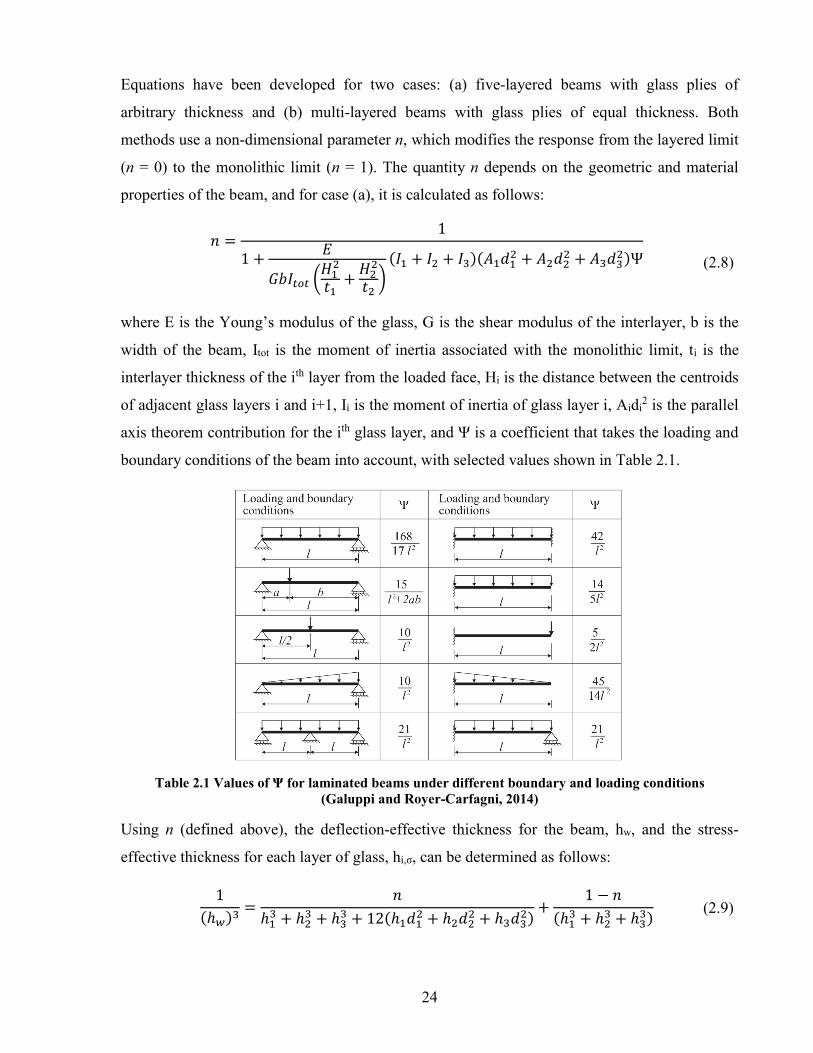
24

Equations have been developed for two cases: (a) five-layered beams with glass plies of

arbitrary thickness and (b) multi-layered beams with glass plies of equal thickness. Both

methods use a non-dimensional parameter n, which modifies the response from the layered limit

(n = 0) to the monolithic limit (n = 1). The quantity n depends on the geometric and material

properties of the beam, and for case (a), it is calculated as follows:

𝑛 =

1

1 + 𝐸

𝐺𝑏𝐼𝑡𝑜𝑡 (𝐻12

𝑡1+ 𝐻2

2

𝑡2)

(𝐼1 + 𝐼2 + 𝐼3)(𝐴1𝑑12 + 𝐴2𝑑2

2 + 𝐴3𝑑32)Ψ

(2.8)

where E is the Young’s modulus of the glass, G is the shear modulus of the interlayer, b is the

width of the beam, Itot is the moment of inertia associated with the monolithic limit, ti is the

interlayer thickness of the ith layer from the loaded face, Hi is the distance between the centroids

of adjacent glass layers i and i+1, Ii is the moment of inertia of glass layer i, Aidi2 is the parallel

axis theorem contribution for the ith glass layer, and Ψ is a coefficient that takes the loading and

boundary conditions of the beam into account, with selected values shown in Table 2.1.

Table 2.1 Values of Ψ for laminated beams under different boundary and loading conditions

(Galuppi and Royer-Carfagni, 2014)

Using n (defined above), the deflection-effective thickness for the beam, hw, and the stress-

effective thickness for each layer of glass, hi,σ, can be determined as follows:

1

(ℎ𝑤)3 =𝑛

ℎ13 + ℎ2

3 + ℎ33 + 12(ℎ1𝑑1

2 + ℎ2𝑑22 + ℎ3𝑑3

2)+

1 − 𝑛(ℎ1

3 + ℎ23 + ℎ3

3) (2.9)

25

1

(ℎ𝑖,𝜎)3 =

2𝑛|𝑑𝑖|ℎ1

3 + ℎ23 + ℎ3

3 + 12(ℎ1𝑑12 + ℎ2𝑑2

2 + ℎ3𝑑32)

+ℎ𝑖

ℎ𝑤3 (2.10)

where hi is the thickness of the ith glass layer and di is the distance between the centroid of the

beam and the centroid of the ith glass layer. The maximum stress in the ith layer can be

calculated by using a monolithic beam of thickness hi,σ under the same boundary and loading

conditions as the laminated beam of interest. The method showed good agreement with three-

dimensional numerical models of multi-layered laminated glass beams for both case (a) and case

(b). The formulations for case (b), and more information on the EET method can be found in

Galuppi and Royer-Carfagni (2014).

2.6 Blast Effects on Glazing The previous sections detailing blast fundamentals and the behaviour of laminated glass

warrant discussion of the effects of blast loading on glazing. With the increased use of glass in

building façades, glazing is often the first line of defense, protecting building occupants and

property from the blast wave. Glazing is also attributed to the majority of injuries in blast

events, due to lacerations, abrasions, and contusions from sharp glass projectiles (Norville,

1999). Thus, understanding the behaviour of glazing under blast loads is critical to the current

research.

2.6.1 Response of Glazing to Blast Loads The primary role of glazing is to create a boundary between the inside and the outside of a

building. When out-of-plane loads are applied to the window, these loads must be transmitted by

the glazing to the main structural system of the building. Due to the brittle nature of glass,

windows are often the weakest component of a structural system. Depending on the glass type,

shards of varying shapes and sizes will be created when the pane fails, and, if not laminated,

these fragments will enter the protected space. When a monolithic glass pane fails, loads from

the blast wave are no longer transmitted to the framing system, as it is able to vent into the

protected space. A unique design problem is introduced when laminated glass is used, as care

must be taken to design a framing system able to withstand much higher loads, as venting no

longer occurs.

Traditionally, the negative phase of the blast load is ignored in design, as, in most cases, it

has little effect on the structure (USACE, 2008). This has been proven otherwise for glazing.

26

Krauthammer and Altenburg (2000) showed that, for some scaled distances, the negative phase

produced large deflections, which could cause a pane to fail even if it remained intact during the

positive phase. Additionally, the negative phase is responsible for pulling glass fragments out of

the building into the nearby area, increasing the potential for injuries and damage.

2.6.2 Blast-Resistant Glazing Design The failure of monolithic annealed glass windows under blast loading represents a high

hazard to building occupants due to both the formation of sharp glass projectiles and the

admittance of the blast wave into the protected space. Different technologies are available to

improve the performance of glazing subjected to blast loads.

When new-build applications are considered, laminated glass windows are by far the best

choice when designing for blast loads. As previously mentioned, glass fragments remain bonded

to the interlayer material when the glass cracks, reducing the potential of injury from flying

glass projectiles. When properly designed, the interlayer does not tear under the applied load,

and it acts as a barrier between the building interior and the blast wave. Designers can also

choose to use heat-strengthened or tempered glass in the layup, as both types of glass can

withstand higher loads than their monolithic counterparts.

Retrofitting is an option when the blast resistance of an existing glazing system needs to be

increased. Anti-shatter films, applied to the protected side of a window, hold the glass fragments

together after the pane has cracked. The film can be anchored to the window frame

mechanically or with structural silicone for additional protection. Bomb-blast curtains, another

retrofit, act as a net to catch panes that have been ejected from their frames. There are typically

used in conjunction with anti-shatter film, as loose glass shards could potentially cut the curtain

fabric. Bomb-blast curtains are not popular, however, as they reduce visibility and ventilation

and are aesthetically unpleasing (Cormie et al., 2009).

2.6.3 Testing Methods for Glazing Subjected to Blast Loads Experimentation is considered the easiest and most reliable way to determine the resistance

of a glazing system to varying blast load intensities. One of two methods is typically used: arena

blast testing or shock tube testing. In an arena blast test, specimens, often referred to as targets,

are mounted in a reaction structure. An explosive charge is placed a set distance away from the

target. The charge weight and standoff can be altered to achieve the desired scaled distance,

which determines the blast wave parameters, previously discussed in Section 2.1.2.

27

A shock tube, on the other hand, utilizes compressed gas to simulate a blast. The tube is

split into two sections by a diaphragm, which is designed to burst at a pre-determined pressure.

One side of the tube is filled with air and failure of the diaphragm causes the higher-pressure gas

to move rapidly into the lower-pressure section, forming a shock wave. The specimen to be

tested is placed at the end of the lower-pressure section.

There are advantages and disadvantages associated with both testing methods. Arena blast

tests better simulate actual blast conditions, but it is difficult to create consistent blast waves,

even when the scaled distance and explosive remain unchanged. Shock tube tests produce more

consistent shock waves and are less expensive. However, it is difficult to reproduce the negative

phase of a blast and specimen size is limited to the dimensions of the shock tube.

Both testing methods have been adopted in testing standards for blast-resistant glazing in

North America and Europe. Procedures for arena blast tests can be found in ASTM F1642

(ASTM, 2012b), BS EN 13123-2/BS EN 13124-2 (BSI, 2004a, 2004b), ISO 16933 (ISO,

2007a), and GSA TS01 (GSA, 2003). Shock tube tests are covered by BS EN 13123-1/BS EN

13124-1 (BSI, 2001a, 2001b) and ISO 16934 (ISO, 2007b). Each testing standard details

requirements for the specimen and reaction structure, as well as charge weight and standoff

distance. Instrumentation and data collection requirements are also specified, including, but not

limited to, pressure-time histories of the blast wave, ambient conditions at the time of testing,

and condition of the specimen post-test. This research focusses on the arena blast test method of

collecting experimental data. A comprehensive comparison of testing standards has been

undertaken by Walker et al. (2012).

While the goal of blast testing is to collect quantitative information describing the

behaviour of a glazing system subject to such loads, the variability of shock waves from the

same explosive, combined with instrumentation failure, does not always allow direct

comparison between tests. A standard reaction structure, or test cubicle, has been defined which

allows different glazing systems to be qualitatively compared instead. The cubicle is 10 feet

long, and a sheet called a witness panel is attached to the back face of the cubicle to collect glass

fragments. Different glazing systems can then be compared based on how far fragments are

thrown into the cubicle under similar blast loads. The performance standard, GSA TS01 (GSA,

2003), is the most common standard used for this purpose. This standard divides the cubicle into

different zones, as shown in Figure 2.9, and each zone is assigned a hazard rating. The GSA

TS01 performance criteria are outlined in Table 2.2. After a test is conducted, the test cubicle

floor and witness panel are examined to determine the maximum hazard level for that glazing

28

system under the specified load. Other aforementioned standards include similar performance

criteria; however, their use is not widespread like GSA TS01.

Figure 2.9 GSA TS01 test cubicle (GSA, 2003)

Performance Condition

Protection Level

Hazard Level Description of Window Glazing Response

1 Safe None Glazing does not break. No visible damage to glazing or frame.

2 Very High None Glazing cracks but is retained by the frame. Dusting or very small fragments nears sill or on floor acceptable.

3a High Very Low Glazing cracks. Fragments enter space and land on floor no further than 3.3 ft. from the window.

3b High Low Glazing cracks. Fragments enter space and land on floor no further than 10 ft. from the window.

4 Medium Medium Glazing cracks. Fragments enter space and land on floor and impact a

vertical witness panel at a distance of no more than 10 ft. from the window at a height no greater than 2 ft. above the floor.

5 Low High Glazing cracks and window system fails catastrophically. Fragments

enter space impacting a vertical witness panel at a distance of no more than 10 ft. from the window at a height greater than 2 ft. above the

floor.

Table 2.2 GSA performance conditions for window system response (GSA, 2003)

2.7 Modelling Analytical and numerical methods are required to predict the behaviour of laminated glass

under blast loads, due to the complexity of both the load and structural response. This section

outlines different methods for determining the behaviour of laminated glass to out-of-plane

loads, including thin and thick plate theory, as well as single-degree-of-freedom and explicit

finite element modelling.

29

2.7.1 Plate Theory A plate is a flat structural element with a thickness much smaller than its other dimensions,

such as a glass ply. Plates can be classified in three categories: thin plates with small deflections,

thick plates, and thin plates with large deflections. A plate is labelled thin when its thickness is

less than 1/20th of the smaller span. Kirchhoff developed classical plate theory for isotropic,

homogeneous, elastic, thin plates and outlined four basic assumptions: (1) the midsurface

deflection is small compared to the thickness of the plate; (2) the midplane remains unstrained;

(3) plane sections remain plane, and thus the shear strains are negligible; and consequently (4)

shear stress is small relative to the other stress components and can be neglected. These

assumptions are analogous to the assumptions made in the bending theory of beams. Kirchhoff’s

theory can simplify a 3-dimensional problem into a 2-dimensional one, and it can be applied to

many engineering applications. In contrast, shear stresses are important in thick plates and both

assumptions (3) and (4) are invalid, and thus, in thick plate theory, transverse shear stresses are

accounted for (Ugural, 2009). When a thin plate undergoes large deflections, assumptions (1)

and (2) above are no longer valid, and the relationship between external load and deflection is

no longer linear. Large deflections cause the midplane to stretch, causing it to develop tensile

membrane forces. These membrane forces can add load-carrying capacity to the plate and are

fully realized when a plate has fixed-edge supports. When the deflection of the plate is equal to

its thickness, the membrane action is comparable to the bending action. For values of deflection

greater than the plate thickness, membrane action governs the response. Although termed large

deflection, the plate deflection still remains significantly less than the other dimensions of the

plate (Szilard, 2004). Research has shown that glass plies undergo large deformation due to out-

of-plane loading, and thus they must be treated as thin plates with large deflections,

superimposing the in-plane bending stresses with the membrane stresses. The material of the

glass plate remains linear elastic, and the nonlinear behaviour is a result of geometric

nonlinearities (Vallabhan et al., 1990). Due to the nonlinearity of the force-displacement

relationship, describing the behaviour of glass plates requires solving differential equations.

Closed-form solutions for stresses and displacements have been derived for basic conditions,

such as a rectangular, simply-supported plate (Szilard, 2004). When closed-form solutions do

not exist, or loading conditions are complex, such as in blast loading, numerical modelling can

be used.

30

2.7.2 Single-Degree-of-Freedom Modelling Structural components experiencing dynamic loading can be simplified and modelled as a

single-degree-of-freedom (SDOF) system, consisting of a mass, a spring, and a damper. In the

case of blast loading, damping is generally ignored, as it has little influence on the first peak

displacement, which is often the response parameter of greatest interest (USACE, 2008). There

are two main SDOF approaches: the modal method and the equivalent SDOF method. Both

methods are similar, assuming the response of one point along the distributed member

represents the response of the entire system. The response at any one point is equated to that of

an idealized lump mass-spring system that has exactly one displacement variable (Morison,

2006).

The modal method was first published in 1946 in EM 1110-345-405 “Fundamentals of

Protective Design (Non-Nuclear)” and later reissued in 1965 as TM5-855-1 (DA, 1965). This

method assumes that the elastic forced response of a member is approximated by the first mode

of vibration, and its period is equal to the period of first mode of vibration. Charts were initially

developed for simply-supported beams exposed to different idealized loading functions, where

maximum deflection and time of maximum deflection could be determined. Later, charts for

other member types and support conditions were developed. Over time the modal method was

replaced by the equivalent SDOF, due to its lack of versatility and its unsatisfactory treatment of

reaction forces (Morison, 2006).

The equivalent SDOF method was developed after the modal method. EM 1110-345-415

“Principles of Dynamic Analysis and Design” (USACE, 1957) was one of the first documents to

present the theoretical basis behind the method. In brief, the mass, resistance, and loading of a

structural element are replaced by equivalent values for a lumped mass-spring system, using

transformation factors. Thus, the equation of motion is as follows:

𝐾𝑀𝑚�̈� + 𝐾𝐿𝑘𝑦 = 𝐾𝐿𝐹(𝑡) (2.11)

where m, k, and F(t) are the actual mass, stiffness, and applied load, respectively; KM and KL are

the equivalent mass and load factors; and ÿ and y are the central-pane acceleration and

displacement. The transformation factors are determined based on the principle of energy

conservation. The equivalent mass has equal kinetic energy, the equivalent resistance has equal

strain energy, and the equivalent load has equal external work to the distributed system.

Transformation factors are a function of the distributed mass and load, as well as the shape

31

function of the deflected element. The accuracy of this method is contingent on the assumed

deflected shape. Provided that the deflected shape is consistent with the support conditions, the

approximation should be suitably accurate. It has been shown that the mode shape for

fundamental free vibration, along with the static deflected shape, both give reasonable results.

Finally, different transformation factors are required for the different stages of deformation of

elastic-plastic members, which reflect the changes in stiffness and strength. These factors can be

derived through the use of plate theory equations or, for common loading and boundary

conditions, they can be found in tables such as those in Biggs (1964). For elements with non-

linear stiffness, a static resistance function determined experimentally may be required. There

are many methods available for solving the equation of motion, but the favoured method is to

solve it numerically in a step-by-step process outlined by Biggs (1964). This allows for the most

flexibility and, in the interest of this research, the ability to use complex resistance functions

(Morison, 2006).

SDOF modelling has been used by researchers to predict the overall behaviour of laminated

glass. Fischer and Häring (2005) used simplified elastic and elastic-plastic resistance functions

to model the behaviour of laminated glass under blast loading, and the experimental data fitted

poorly to the SDOF output. They found that a tri-linear resistance function produced much

better results. Morison (2006) also used the equivalent SDOF model, focussing heavily on the

properties of PVB, and he modified some transformation factors from Biggs. Wedding (2010)

used a resistance function determined by the program HazL and found good correlation between

experimental and model results for laminated windows. Ideally, the static resistance function

would be determined experimentally for more precision. Finally, Zhang et al. (2015b) also

compared field-blast-tested laminated glass windows with SDOF models from both Biggs and

Morison, with varying levels of agreement. It follows that the application of SDOF models can

be extended to predict the behaviour of multi-layered laminated glass windows, provided that

the resistance function is determined experimentally.

2.7.3 Finite Element Method The Finite Element Method (FEM) is a numerical method best suited for solving problems

with complex geometry, loadings, or material properties, which make analytical solutions

difficult or impossible to obtain. Using the FEM, designers can model these complex problems.

The models undergo discretization, where smaller elements with connecting nodes are created.

A series of equations is solved for each node, until a stable solution is produced.

32

ANSYS, ABAQUS, and LS-DYNA are some of the commercial FEM programs available

to designers. The user must fully define the problem, which includes sketching the geometry,

selecting the appropriate material models and failure criterion, meshing the model, and applying

the loading and boundary conditions. FEM software is commonly used by researchers, who use

experimental data to validate their computer models. On the other hand, the FEM is often

considered too time-consuming for routine design work and is reserved for complex design

problems.

2.8 Software Packages Commercial software packages exist to aid structural engineers in designing laminated glass

windows for blast loading applications. Due to the complex behaviour of laminated glass, such

programs are essential. A recent study by Spiller et al. (2016) compared the accuracy of the

following three programs in determining the behaviour of monolithic annealed glass under blast

loading, giving insight into their potential accuracy when applied to multi-layered laminated

glass windows. The findings of the study with regards to each program will be detailed below.

2.8.1 SBEDS The Single-Degree-of-Freedom Blast Effects Design Spreadsheet (SBEDS) (USACE, 2009)

is an Excel-based program that was developed by Baker Engineering and Risk Consultants for

the U.S. Army Corps of Engineers Protective Design Center. The program is used to design

structural components subjected to dynamic loading using single-degree-of-freedom (SDOF)

methodology. The intended users of SBEDS are structural engineers with experience in

structural dynamics and blast loading. It meets Department of Defense (DoD) antiterrorism

standards, specifically UFC 4-010-01 “Minimum Antiterrorism Standards for Building”.

SBEDS can also be used for more general structural dynamics problems as described in UFC 3-

340-02 “Structures to Resist the Effects of Accidental Explosions” (Polcyn & Myers, 2010).

SBEDS has 12 predefined structural components that the user may select for dynamic

analysis. The user inputs all the geometric and material properties necessary to define the

component, and SBEDS then calculates the required SDOF system properties, including mass,

stiffness, and resistance. End supports can either be simply-supported or fixed, and target size

and incident angle can be entered manually to accurately determine clearing and reflection

effects. Furthermore, tension membrane action can be considered together with flexural

response. Finally, the user can also define the percent of critical damping for the analysis. In

33

addition to the 12 predefined components, a general SDOF option is also available. Here, the

user inputs their own resistance function, including KLM factors. Up to five inbound

displacement-resistance pairs can be input into the spreadsheet.

Blast loads are input into SBEDS in one of three ways. The “manual” method lets users

input up to eight time-pressure pairs to define the pressure-time history of the blast. The “charge

weight and standoff distance” option assumes a hemispherical surface burst and calculates the

pressure-time history using scaled curves from UFC 3-340-01 and UFC 3-340-02. This method

also allows users to specify whether or not to include the negative loading phase. Finally, the

“pressure-time history file” method allows users to input a data file with up to 2,000 time-

pressure pairs.

SBEDS uses the constant velocity method, also known as the acceleration impulse

extrapolation method, to perform numerical integration to solve the equation of motion. In

general, the program uses the SDOF equivalency factors suggested by Biggs (1964). Some

changes have been made to the factors for two-way components, due to recommendations by

Morison (2006) (Polcyn & Myers, 2010). In order to solve the equation of motion for each of

the 12 predefined components, SBEDS uses a general resistance-deflection relationship that can

take up to five stiffness regions for inbound and rebound motion. A very small time step is

required for SBEDS to work properly to avoid overshooting the correct solution (USACE,

2008). After the analysis is run, results are shown in graphical form in terms of time, including

displacement, applied load, resistance, and dynamic shear. The resistance function is also

plotted. The above data, as well as velocity and acceleration, are also output in tabular form. In

addition to solving the equation of motion, SBEDS can also produce pressure-impulse diagrams.

The version of SBEDS (Version 4.1) used for this research does not have a predefined

glazing option. Another program, SBEDS_W, has been developed to fill this void. This program

can analyze laminated, filmed, annealed, heat-strengthened, and fully-tempered glazing in

single-pane or double-pane windows under blast loads. Due to distribution restrictions,

SBEDS_W is unavailable for use in this research.

Spiller et al. (2016) utilized both the metal plate component and the general SDOF to model

monolithic annealed glass panes. It was found that SBEDS was able to predict the behaviour

reasonably well when the general SDOF option was used, as it allowed a custom resistance

function, based on experimentation, to be input into the program. The shape of the displacement

curve output by SBEDS closely matched the displacement data collected in the field, although

the program was less accurate at determining the time of pane failure.

34

2.8.2 WINGARD WINdow Glazing Analysis Response and Design (WINGARD) (ARA, 2010a) is a software

program that was designed by Applied Research Associates (ARA) and commissioned by the

US General Services Administration. Unlike SBEDS, WINGARD is specific to glazing, and it

has become the standard for the analysis of glazing systems under blast loads. The professional

edition (WINGARD PE) uses SDOF methodology to determine the behaviour of a wide variety

of user-defined glazing systems (ARA, 2010b).

WINGARD uses a system of libraries for each input parameter. Users can either use the

default entries or add their own. The charge library stores both pressure and impulse TNT

equivalencies for many different charge types. Next, the film, laminate, and glass libraries

contain information regarding the material properties of each layer type. The airblast library

enables users to input either a linear equivalent or a time-pressure history to define the blast

event. The linear equivalent method uses two values, peak pressure and load duration, while the

time-pressure history method allows users to input a series of time-pressure pairs. Finally, the

layup library allows users to combine the layers defined previously (in the film, laminate, and

glass libraries) into glazing layups, composed of panes, plates, and layers. Plates are comprised

of alternating layers of glass and laminate, and they are assumed to act in a composite fashion.

Adjacent plates are considered stacked, with no horizontal shear transfer between them. Panes

are made up of plates, separated by air gaps, and each pane moves independently (ARA, 2010b).

After the user has input all of the required library items, they define a window system,

which combines an airblast with a layup. The window dimensions are specified, including the

height above the ground as well as the frame bite. The airblast is either selected from the airblast

library, or manually entered as a charge weight and standoff distance. When using the manual

option, the user chooses either the pressure or impulse TNT equivalency. They also specify the

curve shape: linear, Friedlander, or Friedlander with clearing. Finally, the edge conditions are

specified. The user can choose butt glazing or wet glazing, although WINGARD warns that the

implementation for wet glazing has not been sufficiently validated.

As ARA no longer releases the technical manual for WINGARD, it is difficult to determine

what assumptions are made during analysis. However, Morison (2007) has outlined some of the

main features of WINGARD. The program uses the SDOF coefficients defined by Biggs (1964)

and glass resistance is calculated after Moore’s theory (1980). WINGARD utilizes a closed-

form, non-linear equation for elastic membrane resistance, calculated by equating strain energy

35

and work done. An elastic-pure plastic membrane resistance was introduced in later versions,

but its accuracy has been questioned (Morison, 2007). Finally, damping is defined as a

proportion of critical damping with a default value of 2%.

Once the program has run, there are numerous outputs for the user to review that are

relevant to glazing design. Graphs depicting central pane displacement, velocity, and

acceleration are plotted, as well as resistance and dynamic reactions. All plots can be exported

as DPlot files for further study. In addition, an analysis text is produced which outlines the input

parameters and summarizes the outputs, including the time of failure for each layer, the

maximum central pane displacement, and velocity at failure. WINGARD predicts the fragment

flight path for all window systems and assigns a hazard rating. Finally, the program uses the

specified bite and pane deflection to determine if the pane will fall out of its support.

For the case of monolithic annealed glass panes, Spiller et al. (2016) found that WINGARD

outputs generally matched closely with the experimental data, specifically the predicted

displacement at failure. However, WINGARD underestimated the GSA hazard ratings for some

of the tests.

2.8.3 CWBlast Curtain Wall Blast (CWBlast) is an explicit finite element program designed specifically for

the analysis of various glazing systems subject to blast loading (Seica et al., 2011). The program

was developed at the University of Toronto and, as of yet, is not commercially available. The

goal of CWBlast was to develop a user-friendly, fast-running finite element software (Krynski,

2008). It has been validated with both static and dynamic experimental data with good results

(Seica et al., 2011).

CWBlast gives the user full control over all of the properties of the glazing system. First,

the user defines the height and width of the window, as well as the height of the sill. Then, the

window layup is entered. Default material properties for annealed glass, heat-strengthened glass,

tempered glass, polyvinyl butyral, and ionoplast are provided, but the user may modify the

values or create their own custom material. Monolithic, laminated, and insulated glass units with

up to two plates can be modelled. Next, the support conditions are selected. CWBlast offers

eight different options for boundary conditions, as shown in Figure 2.10, giving the user

flexibility when modelling the glazing system. After the window system has been fully defined,

the user has three options for inputting the blast load: charge weight and standoff, peak pressure

and impulse, or time-pressure pairs. The first two options model the shock wave as an

36

equivalent triangular load, and thus, do not let the user model the negative phase of the blast.

The user can also specify the area of the pane that experiences the blast load, representing

scenarios where the window may be partially blocked.

Figure 2.10 CWBlast support condition options

Four-noded isoparametric quadrilateral elements with five degrees of freedom per node, and

bilinear Lagrangian shape functions are used with 2 x 2 numerical integration. A variation of the

Newmark-Beta method is used to calculate transient displacements, while thick, or Mindlin,

plate theory is used to determine the plate stresses. The user can decide whether to include

geometric nonlinearity and symmetry conditions in their solution. The program suggests both

the number of elements to use and the time step for the analysis, although the user can use

custom values. Failure of the plate is determined in one of two ways, either using the maximum

principal stress method, or the Glass Failure Prediction Model, which takes surface flaws into

account (Seica et al., 2011).

CWBlast outputs data similar to WINGARD, all of which are pertinent when designing

blast-resistant glazing. Central pane displacement, maximum principal stress, and the blast load

are output in both tabular and graphical form. Other parameters, including pane velocity and

pane acceleration are output only in tabular form. Data is calculated for the entire pane, in order

to capture the maximum tensile stress, which, due to plate bending, may not occur at the centre.

The GSA hazard rating is determined based upon the displacement, velocity, and acceleration of

the pane at the moment of failure. Unlike WINGARD, CWBlast does not output the dynamic

edge reactions, which aid in frame design.

Spiller et al. (2016) determined that CWBlast was more accurate when the Glass Failure

Prediction Model was used, as opposed to the maximum principal stress method, provided the

Weibull parameters matched the glass being used.

37

3 Field Blast Testing Full-scale field blast tests on multi-layered laminated glass windows were conducted in

2015 in conjunction with DNV-GL at the Spadeadam Testing and Research Centre in the United

Kingdom. The purpose of this test series was to collect experimental data to determine the

applicability of Single-Degree-of-Freedom (SDOF) analysis for multi-layered laminated

windows under blast loading. Field testing consisted of two arena blasts of nitromethane

equivalent to 400 kg of trinitrotoluene (TNT), each at a different scaled distance. Two unique

glass compositions were tested with two panes of each composition per blast, for a total of eight

tested specimens. The test series was conducted with the support of the Explora Foundation.

3.1 Targets and Reaction Structure The targets for this test series consisted of two different multi-layered laminated glass make-

ups, designated ‘old’ and ‘new’, which are described below in Table 3.1. Each glass specimen

measured 1300 mm by 700 mm, with a thickness of approximately 42 mm. The laminated glass

targets were installed in steel frames with Dow Corning 121 Structural Glazing Sealant (Dow

Corning, 2015), creating a wet-glazed system. All panes were installed with silicone beads on

both faces of the window. The structural bite was 50 mm, and the silicone bead width occupied

the full bite, resulting in clear dimensions of 1200 mm by 600 mm for the glass targets.

Layer Name Old New THREAT SIDE

G1 10 mm Annealed Glass 6 mm Heat-Strengthened Glass L1 1.52 mm PVB 1.52 mm PVB G2 8 mm Annealed Glass 8 mm Heat-Strengthened Glass

L2 1.52 mm PVB 1.52 mm PVB G3 8 mm Annealed Glass 8 mm Heat-Strengthened Glass L3 1.52 mm PVB 1.52 mm PVB G4 6 mm Annealed Glass 10 mm Heat-Strengthened Glass L4 1.52 mm PVB 1.27 TPU P1 4 mm Polycarbonate 4 mm Polycarbonate

PROTECTED SIDE Table 3.1 Multi-layered laminated glass window compositions

Both the old and new compositions consisted of nearly the same layers of glass and

interlayer. The primary difference between the two make-ups was the order of the layers.

Specifically, the 10 mm pane is located nearest the threat in the old composition and nearest the

protected face in the new. All four specimens for each test were mounted on a single reaction

38

structure. Figure 3.1 indicates the naming convention for each specimen, with the first letter (O

or N) representing the Old or New window composition (see Table 3.1); T# representing Test 1

(T1) or Test 2 (T2); and S1 and S2 representing Specimen 1 and Specimen 2.

Figure 3.1 Specimen naming convention – outside view

The reaction structure consisted of a welded steel frame constructed from “universal

column” (I-shaped) sections, which was anchored to a one-metre-deep concrete culvert section.

The steel frame had four openings, which measured 1200 mm by 600 mm, identical to the clear

dimensions of the targets. Each target was attached to the outside face of the steel frame with 14

perimeter M16 through bolts. Two additional culverts were placed behind the first culvert,

creating a test cubicle that was approximately 3 m deep, as per GSA TS01 (GSA, 2003)

standards (Figure 3.2). Another two culverts were placed on either side of the reaction structure

to minimize any clearing effects. Plywood sheets were installed on the front face to close any

39

gaps that existed between the steel columns and the culverts. The plywood was installed in an

attempt to provide a uniform reflecting surface for the shock front. The complete setup can be

seen in Figure 3.3.

3.2 Testing Methodology Two different window compositions were tested side-by-side at two different scaled

distances which allowed their performance to be compared directly. Due to the numerous layers

of glass and interlayer, the standoff distances were relatively small compared to other single-

layer laminated glass test series (Hooper et al., 2012b; Zhang et al., 2015b). The expected

pressure and impulse values, as predicted from the UFC-3-340-02 blast parameter scaling chart

for hemispherical charges (DoD, 2008), were on average four to eight times higher than these

previously performed tests. The 2015 test details can be seen in Table 3.2, including charge

weight and standoff distance, as well as the atmospheric conditions at the time of the test.

WINGARD (ARA, 2010) was used to determine the standoff distances required based on the

level of damage that was desired for each test.

Test Standoff (m)

Charge (kg TNT equivalent)

Scaled Distance (m/kg1/3)

Temp (qC)

Humidity (%)

Pressure (kPa)

1 19 400 2.58 12.0 88 100.3 2 15 400 2.04 14.0 63 101.7

Table 3.2 Test details

A spherical charge of nitromethane equivalent to 400 kg of TNT was used in each test, using an

equivalency factor of 1.094. This translates into 361.6 kg of nitromethane and 4 kg of PE4 for

400 kg of TNT. While arena testing facilities in the UK use an equivalency of 1.094, recent tests

have shown that the actual equivalency is likely between 1.2 and 1.4. This conversion was not

conclusive, and as such the value of 1.094 is still being used so that past and future test results

using nitromethane can be compared (Bougard, 2003). The plastic charge casing measured 860

mm in diameter, the centre of which was positioned 1.6 m above the concrete test pad on a

polystyrene block, which in turn sat on a 75 mm thick steel plate. The reaction structure was

placed at the edge of the test arena, and the charge was located at the standoff distance listed in

Table 3.2. Pressure gauge blocks were stacked one on top of another to achieve a similar height

40

Figure 3.2 Side view of reaction structure with glass targets installed

Figure 3.3 Front view of reaction structure with targets installed

41

and width to the reaction structure, and these blocks were erected at the same standoff distance

as the target. Figure 3.4 shows the test arena setup for Test 1, with the pressure gauge blocks

shown on the left, the charge in the middle, and the reaction structure on the right.

Figure 3.4 Test arena setup – Test 1

3.3 Instrumentation The targets and the blast test arena were fully instrumented in order to quantify the blast

load as well as the response of the windows to this load. The blast wave parameters were

measured using the aforementioned pressure gauge blocks as well as a stand-alone free-field

gauge, located at the same standoff as the target. Three PCB B21 gauges were placed in the

pressure gauge blocks. One was located at the mid-height of the lower windows, and the other

two were located at the mid-height of the upper windows. For Test 2, unlike in Test 1, the free-

field gauge was anchored into the test pad to ensure it remained upright.

Each pane was equipped with a LVDT to measure its peak out-of-plane displacement at the

centre point of the pane. In Test 1, the LVDTs were attached to the polycarbonate with an

adhesive pad, however this proved to be an ineffective way to mount the gauges to the

polycarbonate, and three of the four gauges disconnected during Test 1. To counteract this in

Test 2, the LVDTs were attached using a two-part epoxy. In addition, Baumer Electric laser

displacement gauges were used in Test 2 to add redundancy for the displacement readings. The

displacement gauges were mounted on steel angles that were anchored to the first concrete

culvert, as shown in Figure 3.5.

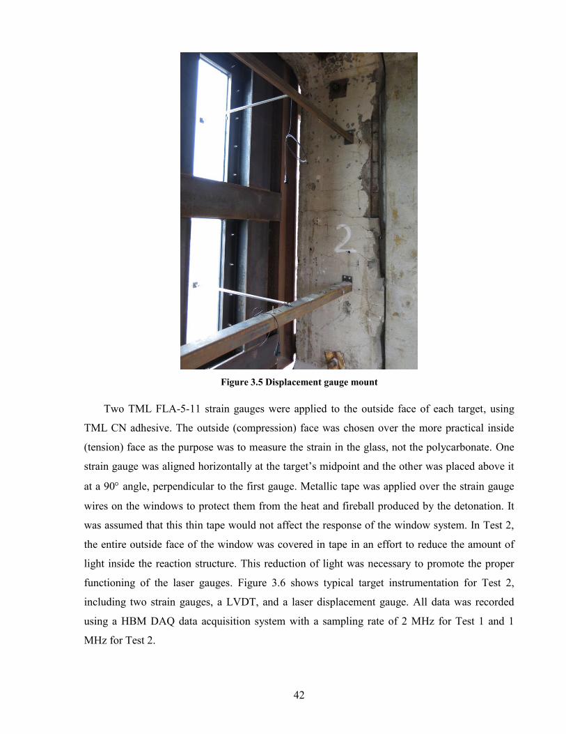
42

Figure 3.5 Displacement gauge mount

Two TML FLA-5-11 strain gauges were applied to the outside face of each target, using

TML CN adhesive. The outside (compression) face was chosen over the more practical inside

(tension) face as the purpose was to measure the strain in the glass, not the polycarbonate. One

strain gauge was aligned horizontally at the target’s midpoint and the other was placed above it

at a 90q angle, perpendicular to the first gauge. Metallic tape was applied over the strain gauge

wires on the windows to protect them from the heat and fireball produced by the detonation. It

was assumed that this thin tape would not affect the response of the window system. In Test 2,

the entire outside face of the window was covered in tape in an effort to reduce the amount of

light inside the reaction structure. This reduction of light was necessary to promote the proper

functioning of the laser gauges. Figure 3.6 shows typical target instrumentation for Test 2,

including two strain gauges, a LVDT, and a laser displacement gauge. All data was recorded

using a HBM DAQ data acquisition system with a sampling rate of 2 MHz for Test 1 and 1

MHz for Test 2.

43

Figure 3.6 Test 2 target instrumentation, from interior of window

High-speed video cameras and GoPro video cameras were used in both tests to record video

footage of the panes, instruments, and blast wave. One high speed video camera filmed the

reaction structure from the outside and two GoPro cameras were placed inside the reaction

structure. In Test 1, three additional GoPro cameras were placed around the test arena to capture

the behaviour of the gauge blocks. In Test 2, a drone was also used to capture aerial footage of

the entire blast arena before, during, and after the test.

Finally, foam witness panels covered with thin sheets of paper were placed inside the

reaction structure to collect any glass fragment projectiles from fractured panes.

3.4 Initial Observations Following each test, the targets and test arena were examined for qualitative information. In

Test 1, both of the old-composition windows showed signs of failure, as shown in Figure 3.7.

The crack pattern of O-T1-S2 matched Yield Line Theory for a simply-supported rectangular

slab (Megson, 2014), while O-T1-S1 had a radial crack pattern. Glass layers G2, G3, and G4

(counted from the attack side) showed damage, while glass layer G1 (on the attack side) and the

polycarbonate layer (on the protected side) both appeared damage-free. No fragments or dust

entered the test cubicle, corresponding to US General Services Administration Performance

44

Condition 2 (GSA, 2003). In contrast, neither of the new-composition windows showed any

signs of damage, thus corresponding to GSA Performance Condition 1. Due to the extreme force

of the blast, many of the instruments did not perform as anticipated: the free-field pressure

gauge fell over onto its side; three of the four LVDTs disconnected from the targets; seven of

the eight wires connected to the strain gauges were severed; the external GoPro cameras were

knocked over; and the foam witness panels were ripped off the back wall and obstructed the

internal GoPro cameras as they fell into the 3 m deep cubicle.

Figure 3.7 O-T1-S2 (left) and O-T1-S1 (right)

Before Test 2, much was done to prevent repeating the aforementioned instrumentation

failures (see 3.3 Instrumentation); however, many of the same problems remained. All four

LVDTs detached from the target and all eight strain gauge wires were severed. In terms of target

damage, the polycarbonate layer cracked extensively in both of the new-composition windows

(N-T2-S1 and N-T2-S2). Small glass fragments covered the floor behind the new-composition

windows. Moreover, four fragments from N-T2-S2 were found in the witness panels, while no

shards from N-T2-S1 reached the witness panels. Thus, N-T2-S1 and N-T2-S2 had GSA

Performance Conditions of 3b and 4, respectively. The polycarbonate layer cracked mildly in

the top old-composition window (O-T2-S2) and glass debris was on the floor behind the target,

corresponding to a GSA Performance Condition of 3b. No damage to the polycarbonate layer

45

was observed in the bottom old-composition window (O-T2-S1), resulting in a GSA

Performance Condition of 2. Figure 3.8 shows the targets after Test 2, viewed from inside the

reaction structure.

Figure 3.8 Test 2 old composition (left) and new composition (right), from interior of window

When comparing the qualitative performance of the old and new window compositions, the

new composition performed better in Test 1 (Z = 2.58 m/kg1/3), as no visible damage occurred.

In Test 2 (Z = 2.04 m/kg1/3), the opposite was true with the old windows performing better than

the new. The metric used to gauge the performance of the compositions for the second test was

the final status of the polycarbonate later. Both of the new composition windows exhibited

extensive splitting of the polycarbonate, whereas the old composition showed less or minor

46

damage to the polycarbonate. Based on these qualitative results, there is no definitive answer as

to which composition is preferable. The results indicate that the old composition is more

resistant to damage at lower scaled distances while the new composition is more resistant at

larger scaled distances. However, for both types of multi-layered laminated windows there was

little debris inside the reaction structure after testing, thus indicating the protective nature of

such glazing.

3.5 Data Processing Post-processing of the collected data was completed using DPlot (HydeSoft, 2014). Test 1

used a sampling rate of 2 MHz for all instruments, while Test 2 used a rate of 1 MHz. The high

sampling rates introduced noise into the data, which needed to be removed before analysis. Care

was taken to ensure that all key values, such as peak pressure, were preserved. A general

procedure was followed for each set of data: (1) the timescale was adjusted to correspond with

the time of detonation; (2) any random spikes were removed; and (3) a smoothing function was

utilized to reduce any remaining noise. Figure 3.9 shows a typical set of strain data, before and

after processing, for specimen N-T2-S2-H.

Figure 3.9 Raw vs. processed strain data for specimen N-T2-S2-H

3.6 Blast Waves Overall, the data collected to quantify the blast waves was satisfactory. However, in both

tests, only one reflected pressure gauge (RP3) recorded both the positive and negative phases.

The other two gauges (RP1 and RP2) stopped recording data in the positive pressure phase.

Despite the shortened recording period, the peak positive pressure readings from the three

47

gauges were in relatively good agreement, as indicated in Table 3.3. The free-field pressure data

from both tests was much noisier than the data from the reflected pressure gauges, however it

was still possible to determine definitive peak pressure values from the free-field data. Table 3.3

summarizes the peak pressure and peak positive impulse values for Test 1 and Test 2.

Peak Positive Pressure (kPa) Peak Positive Impulse (kPa-ms) Test RP1 RP2 RP3 RP3* FF1 RP1 RP2 RP3 RP3* FF1

1 577 570 578 497 230 - - 1774 1855 681 2 1135 1218 1422 1237 384 - - 2520 2385 852

Table 3.3 Blast wave peak positive pressure and impulse values RP is reflected pressure, FF is free-field pressure, and * indicates Friedlander fit values

Two slightly more involved methods were employed when processing the pressure data, in

addition to the steps previously mentioned. The first procedure included smoothing the data in

two iterations, using a method described by Ritchie et al. (2014). First, a smoothing window of

50 was used on all the data, and then the peak pressure was determined. This first step removes

noise from the trace while preserving the peak value. The data was further smoothed with a

window of 1,000 from the point of peak pressure, as the data after the peak is less critical. The

second method, applied solely to the reflected pressure data, involved using the Friedlander fit

function in DPlot on the unfiltered data, as per ISO 16933 (ISO, 2007a). Figure 3.10 illustrates

this process for RP3 from Test 1, showing the raw pressure data, the filtered data, and the

Friedlander fit, whose parameters can be seen in Appendix A.

The processed pressure curves were numerically integrated in DPlot using trapezoidal rule

to create impulse-time curves. Finally, the pressure and impulse data was also compared to the

estimated load values from WINGARD, assuming no clearing, as this program was used to

determine the standoff distances for the test series. These values match ConWep outputs for the

same charge weight and standoff distances. An example of this comparison is shown in Figure

3.11. It can be seen from Figure 3.11 that the estimated reflected pressure by WINGARD was

less than what was recorded in the test. After the arrival of the shock front, the pressure values

match very closely for approximately 4.5 ms, after which the recorded pressure dissipates at a

faster rate than the predicted pressure. This resulted in a measured impulse lower than the

predicted value, and similar observations were made for Test 2. In addition, Spiller et al. (2016)

saw comparable discrepancies between predicted and measured reflected pressure values in their

test series on monolithic glass windows.

48

Figure 3.10 Pressure data filtering process - Test 1

Figure 3.11 Reflected pressure and impulse – Test 1

A reason for this discrepancy between the measured and predicted reflected pressure

histories could be that the gauge blocks did not remain in their initial positions. While the final

location of the gauge block was not recorded, in Test 2 the reaction structure was pushed

approximately 70 mm backwards as a result of the blast and it would be reasonable to assume

that the gauge blocks would have moved a similar distance away from the centre of the arena. In

addition, the external GoPro footage showed the blocks rocking back and forth as a unit after the

detonation, which would have facilitated venting through the space between the gauge blocks

and concrete culvert. Clearing around the sides of the gauge block setup likely also occurred. It

49

can be assumed that the reaction structure experienced similar clearing and venting phenomena.

The plywood sheets that were intended to prevent venting between the main reaction structure

and the concrete culverts were pulverized. Similar clearing would have occurred as both

structures had similar geometry. Thus, the discrepancy between the measured and predicted

reflected pressures is of little concern.

As previously mentioned, the charge was elevated 1.2 m above the concrete pad on a

polystyrene block. Thus, the shock-wave front was neither fully hemispherical or spherical. The

average peak positive reflected pressure and impulse values were compared with the estimates

from the UFC-3-340-02 chart for both hemispherical (UFC-H) and spherical (UFC-S) blasts to

see which condition better explained the loading conditions for this test series. As shown in

Table 3.4, the blast waves from the test series are better represented by a hemispherical shock

wave.

Peak Positive Pressure (kPa) Peak Positive Impulse (kPa-ms) Test Average UFC-H UFC-S RP3 UFC-H UFC-S

1 575 501 319 1774 1974 1289 2 1258 1002 614 2520 2620 1701

Table 3.4 Pressure and impulse comparison to UFC-3-340-02

3.7 Displacement-Time Histories Of the eight windows tested, usable displacement data was collected for only two targets,

both of which were old composition windows. In Test 1, three of the four LVDTs disconnected

from the targets. The data from the connected LVDT is presented in Figure 3.12. In Test 2, laser

displacement gauges were added for redundancy purposes. Unfortunately, all four of the LVDTs

detached from the targets, and three of the four laser gauges did not record a peak inbound

deflection, severely limiting the conclusions that could be drawn from the data. The laser gauge

failures could have occurred due to the amount of light that entered the reaction structure, as too

much light can cause the laser gauge to malfunction. Although tape was applied to the outside

surface of the target, which was intended to block out the light, GoPro footage showed that a

significant amount of light still entered the reaction structure when the detonation occurred. The

laser gauge data collected from the single working gauge in Test 2 can be seen in Figure 3.13.

50

Figure 3.12 Measured central displacement – O-T1-S2

Figure 3.13 Measured central displacement – O-T2-S1

Figure 3.12 indicates a peak inbound deflection of about 35 mm and a similar peak of 35

mm during rebound for O-T1-S2. The residual displacement was 3 mm outside of the reaction

structure (not shown in Figure 3.12). The period of oscillation of the broken pane was

approximately 20 ms, measured peak-to-peak and trough-to-trough after the pressure dissipated

(see Figure A.7). It can be assumed that the natural period of the unbroken window would be

less, as the overall stiffness of the system would be greater. Figure 3.13 shows a peak inbound

deflection of 80 mm and a peak rebound deflection of 49 mm for O-T2-S1. The residual

displacement was around 10 mm to the outside of the reaction structure (not shown in Figure

IN OUT

IN OUT

51

3.13), and the period of oscillation was approximately 30 ms. When compared to the period of

oscillation from Test 1, this result is reasonable. The windows in Test 2 experienced more

damage, lowering the system’s stiffness, thus resulting in a longer period of oscillation.

3.8 Strain Rate Strain gauges were applied to the outer (attack) face of the targets to measure the strain rate

experienced at the centre of the window system. The initial strain rate was determined by fitting

a linear equation to the first rapid increase of tensile strain after the blast wave arrived, as shown

in Figure A.9 to Figure A.24 in Appendix A. Only the portion of the strain-time graph before

expected glass cracking was utilized. Table 3.5 summarizes the initial tensile strain rate values

only, as the compressive strength of glass is unaffected by strain rate.

Strain Rate (s-1) Test 1 Horizontal Vertical

O-T1-S1 17.40 11.09 O-T1-S2 3.66 6.11 N-T1-S1 18.7 9.9 N-T1-S2 8.32 11.39 Test 2 Horizontal Vertical

O-T2-S1 14.2 9.8 O-T2-S2 6.8 9.9 N-T2-S1 52.7 11.98 N-T2-S2 9.67 9.47

Table 3.5 Initial tensile strain rate values

The recorded strain rates shown in Table 3.5 are lower than the rates sometimes associated

with blast events, reported as between 102 and 104 s-1 (Ngo et al., 2007), however the strain rate

is dependent on the dynamic characteristics of the structural element under measurement, plus

the scaled distance. The placement of the strain gauges may also have an influence on the

recorded strain rate. In a similar test series, Hooper et al. (2012b) used high-speed 3D digital

image correlation to plot the strain on the inner surface of a laminated glass pane. It was found

that the middle of the pane remained relatively unstrained in comparison to the edges near the

perimeter. This suggests that the chosen location at the centre of the pane may register a lower

strain rate than a position at the perimeter of the pane near the edge, but this would depend on

the boundary conditions and the geometry of the pane.

52

3.9 Limitations and Sources of Error As previously mentioned, many of the instruments did not perform as intended, which

hampered data collection efforts. As the purpose of this test series was to collect experimental

data for the calibration of predictive SDOF models, these instrumentation failures limited the

overall success of the test series. When instrumentation did malfunction, however, it was rather

obvious, and any extraneous data was removed.

3.10 Discussion The test series was considered a minor success in that it gathered substantial qualitative data

and some quantitative experimental data for multi-layered laminated glass windows under blast

loading. Reflected pressure and displacement data were collected for both tests, which provided

enough information to define the blast loads and the approximate response of the panes, which

can be used to evaluate the efficacy of predictive models. The two different window

compositions were qualitatively compared, and it was concluded that while the new composition

performed better in Test 1, the old composition exhibited less damage in Test 2, indicating that

the compositions perform better at different scaled distances. Both window compositions,

however, generated little debris in the reaction structure after testing, demonstrating the

protective nature of multi-layered laminated glass window systems.

In future tests, special care should be taken to ensure that all instrumentation is able to

function as intended, especially when the cost of testing is considered. It is recommended that

future researchers explore using either a grid or speckle pattern on the inner surface of the

window, along with 3D digital image correlation, to better record displacement and strain data

for the entire pane. Non-contact gauges such as lasers and cameras are ideal, because the rapid

nature of the pane displacement can easily disconnect a physical gauge. However, lasers and

cameras must be used in an environment where the level of light is controlled to prevent over-

exposure and faulty readings. If possible, all gauge wires should be protected to avoid damage,

and any cameras and free-field gauges should be anchored securely to the test pad or reaction

structure.

53

4 Laboratory Testing Program Laboratory testing of multi-layered laminated glass beams was completed at the University

of Toronto Structural Testing Facility. The purpose of these tests was to determine the

composite behaviour of the laminates and develop a pressure-displacement resistance function

for use in SDOF analysis.

4.1 Description of Specimens Multi-layered laminated glass beams, with layups matching the old- and new-window

compositions outlined in Table 3.1, were constructed from the same material as the targets in the

arena blast tests. The beams measured approximately 1,500 mm long by 50 mm wide. The edges

of each glass layer were arrissed, a requirement for the heat-treating process. The exact width of

each glass and polycarbonate layer was determined prior to testing, as was the total thickness of

the composite. Individual layer thicknesses were measured from separate 1 m by 1 m sheets of

the layup materials. Average values for both compositions can be found in Appendix B in Table

B.1 and Table B.2. The old- and new-beam cross-sections are shown in Figure 4.1 and Figure

4.2, respectively.

Figure 4.1 Old-composition cross-section (see Table 3.1)

Figure 4.2 New-composition cross-section (see Table 3.1)

54

4.2 Testing Methodology Each beam was tested under a four-point bending configuration. This testing method was

selected in an attempt to capture the critical flaw within the uniformly stressed region between

the two point loads, as failure would be initiated in the zone of constant bending stress. The

support span was 1,250 mm, matching the long-direction span of the field-blasted windows. The

loading span was 500 mm. Both the support and loading spans had one roller support and one

pin support. The test setup diagram is illustrated in Figure 4.3.

Figure 4.3 Test setup schematic (all dimensions in mm)

It must be noted that the chosen loading configuration (i.e. two point loads) differs from the

load applied to the targets in the field (i.e. a uniform pressure). Referencing Galuppi and Royer-

Carfagni (2014) and the EET method, the Ψ factor, an analytical representation for the type of

loading and boundary conditions, for a simply-supported beam under a central point load is

equal to 10/L2 and is equal to 9.88/L2 for a uniformly distributed load, where L is the span of the

beam (see Table 2.1). The Ψ value for a four-point bending configuration would be situated

between these two values, which themselves differ by only 1.2%. Given this small difference, it

was assumed that the four-point bending configuration would be a reasonably representative

method for determining the behaviour of the laminated glass beams experimentally.

Four LVDTs were installed on the test setup to measure the mid-span displacement of the

glass beam, the stroke of the testing machine head and the settlement of the support beam. Strain

gauges were applied at mid-span, on both the top and bottom surfaces of the glass beam, as well

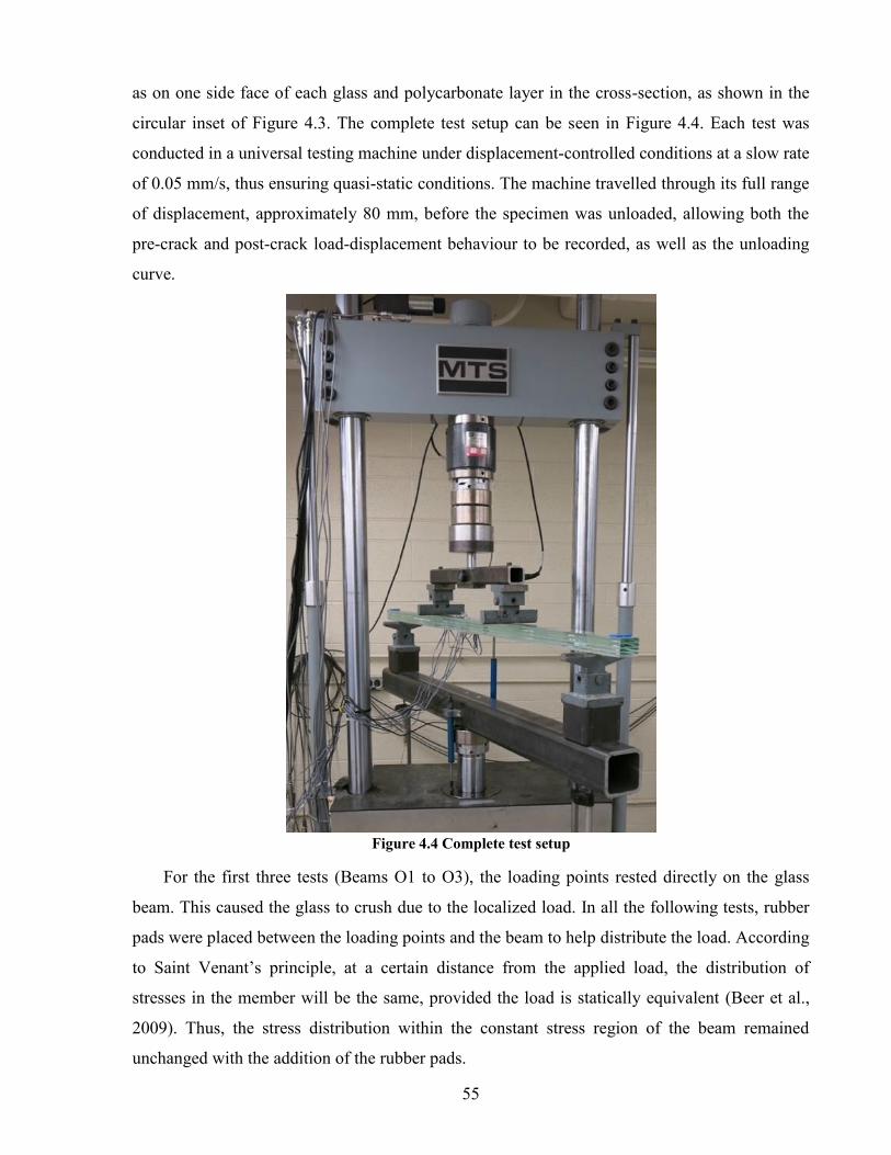
55

as on one side face of each glass and polycarbonate layer in the cross-section, as shown in the

circular inset of Figure 4.3. The complete test setup can be seen in Figure 4.4. Each test was

conducted in a universal testing machine under displacement-controlled conditions at a slow rate

of 0.05 mm/s, thus ensuring quasi-static conditions. The machine travelled through its full range

of displacement, approximately 80 mm, before the specimen was unloaded, allowing both the

pre-crack and post-crack load-displacement behaviour to be recorded, as well as the unloading

curve.

Figure 4.4 Complete test setup

For the first three tests (Beams O1 to O3), the loading points rested directly on the glass

beam. This caused the glass to crush due to the localized load. In all the following tests, rubber

pads were placed between the loading points and the beam to help distribute the load. According

to Saint Venant’s principle, at a certain distance from the applied load, the distribution of

stresses in the member will be the same, provided the load is statically equivalent (Beer et al.,

2009). Thus, the stress distribution within the constant stress region of the beam remained

unchanged with the addition of the rubber pads.

56

For the new-beam tests (Beams N1 to N5), straight vertical lines were drawn on the beam at

the support location. When the loading phase of the test was complete, measurements were

undertaken at this location in order to determine the amount of slip between glass layers and

hence the degree of composite behaviour. Finally, each test was recorded with a high-definition

video camera in order to determine the order in which the individual glass layers cracked.

All tests were conducted at a temperature of 26qC and relative humidity of 16%. The beams

were conditioned in the laboratory for at least 48 hours prior to testing.

4.3 Old-Composition Beams A total of six old-composition beams were tested. Despite the high variability in glass

strength, the load-displacement curves recorded were rather consistent, as shown in Figure 4.5.

The significant values from Figure 4.5 are summarized below in Table 4.1. First-crack load and

first-crack displacement values were calculated by averaging the force-displacement pairs at

first cracking for each beam, whereas the stiffness values were calculated by fitting a linear

curve to each segment of the resistance function.

Figure 4.5 Old-composition force-displacement curve

1st Crack Load (kN)

1st Crack Displacement

(mm)

Initial Stiffness (N/mm)

Secondary Stiffness (N/mm)

Tertiary Stiffness (N/mm)

Residual Displacement

(mm) Mean 1.028 22.7 45.6 29.5 21.6 9.80 Median 1.048 23.2 45.5 30.3 22.0 9.81 SD 0.0563 1.471 0.701 2.09 1.439 0.956 CoV 0.0548 0.0647 0.01539 0.0707 0.0666 0.0976

Table 4.1 Old-composition beam test results

57

As can be seen in Figure 4.5, the load-displacement response of each beam matched almost

perfectly until the displacement at the centre of the beam reached approximately 20 mm. Each

old-composition beam developed its first crack between 20 and 25 mm of displacement, and the

crack was located at, or between, the loading points, in the constant stress region. In general, the

first crack was located in layer G3 or G4 as defined in Table 3.1. Once a single glass layer

fractured, cracks generally propagated quickly through the rest of the cross-section in the region

of the first crack location, as shown in Figure 4.6. When the glass first cracked, the cracks were

small enough that the glass layers above the neutral axis continued to transmit compressive

forces, while tensile forces below the neutral axis were carried by the interlayers and

polycarbonate. The stiffness of the beam decreased by approximately 35% after initial cracking

and 53% after secondary cracking. Initial cracking is defined as the first set of localized

cracking, which was predominately located at one or close to one of the supports. Thus,

secondary cracking is the second set of such cracks. After the secondary drop in load, the beams

continued to carry an increasing load as the displacement was increased, until the maximum

stroke of the universal testing machine was reached. Figure 4.7 shows the crack order for Beam

O6, as determined through video footage.

Figure 4.6 Beam O6 after cracking

Figure 4.7 Beam O6 crack order

58

Even after the glass completely cracked, the beam was able to sustain bending moment due

to the force-couple that developed in the polycarbonate and PVB layers which are braced by the

bonded glass fragments. This is not the case with simply-supported single-interlayer laminated

glass, as a force couple cannot be created once both plies of glass crack. In practice, a laminated

system would be wet-glazed, and thus the horizontal displacement at the supports would be

restrained by the window framing system. In this case, a significant membrane effect would

develop and the window, or beam in this case, would be able to absorb much more strain post-

cracking.

When the beams were unloaded, most of their displacement was recovered, with an average

residual displacement of 9.80 mm, or 0.784% of the span length. From the perspective of energy

absorption capabilities, this result is not ideal. In practice, a blast-resistant window system

should exhibit more plastic, permanent deformation, which occurs during the post-crack phase,

as this would reduce the magnitude of the reaction forces experienced by the support system due

to the increased energy absorption. It is possible that a greater level of plastic deformation

would have occurred had the mid-span displacement been greater, however the tests were

limited in this case by the stroke of the testing machine.

4.4 New-Composition Beams A total of five new-composition beams were tested. The loading behaviour of the new-

composition beams can be seen in Figure 4.8. Due to the higher load-carrying capacity of the

new composition, coupled with the beam’s large deflection, the roller support on the support

span had a tendency to kick outwards at a sudden point in time during the test, effectively

increasing the span of the beam. While the entire load-displacement curve was recorded (i.e.

both the loading and unloading phases), the data was truncated to exclude the behaviour after

the movement of the roller support. The support failure was almost instantaneous, and the time

of movement was recorded and used later to truncate the force-displacement curve. Data of

interest have been extracted from Figure 4.8 and can be found in Table 4.2.

59

Figure 4.8 New-composition force-displacement curve

1st Crack Load (kN)

1st Crack Displacement

(mm)

Initial Stiffness (N/mm)

Secondary Stiffness (N/mm)

Mean 1.614 49.7 32.4 15.48 Median 1.616 50.9 32.1 15.70 SD 0.1098 2.94 0.898 1.545 CoV 0.0680 0.0592 0.0277 0.0998

Table 4.2 New-composition beam test results

The new-composition beams were manufactured from heat-strengthened glass and, as

expected, exhibited higher first cracking loads than the old-composition beams. The average

first crack load was 1.614 kN, 1.57 times larger than the old-composition value. Unexpectedly,

the new-composition beams displayed lower stiffness than their old-composition counterparts:

32.4 N/mm versus 45.6 N/mm, a difference of 33.8%. The reordering of layers was expected to

have a minimal impact on the moment of inertia of the beam (refer to Table 4.3) and heat-

strengthening does not influence the stiffness of individual glass lites (Amstock, 1997).

Additionally, the same interlayer material, PVB, was used in both compositions, except for the

interface between G4 and P1 in the new composition (see Table 3.1). The reason for the

difference in stiffness is not evident, but it is clear that the old- and new-composition beams

display dissimilar composite action and interlayer slip.

The cracking behaviour of the new-composition beams differed from the old-composition

beams. While the cracks in the old-composition beams were localized, the cracks in the new-

composition beams had a tendency to spread out horizontally along the span of the beam, as

60

illustrated in Figure 4.9. This horizontal crack propagation is a by-product of the heat-treating

process, as the first crack locally relieves the strain energy stored from the pre-compression and

the surrounding glass cracks in an attempt to restore equilibrium.

Figure 4.9 Beam N1 crack order and propagation

As mentioned above, straight, vertical lines were drawn on the new-composition beams at

each support location. Photographs were taken at these locations at the end of the loading phase,

an example of which is shown in Figure 4.10, and the photos were scaled and measured in

AutoCAD (Autodesk, 2015) to determine the amount of layer slip. On average, the slip between

adjacent glass layers was around 1 mm. However, there was negligible slip between layer P1

and G4. Here, the PVB interlayer was replaced by TPU, which, as mentioned in Section 2.4.1,

maintains its stiffness at elevated temperatures and thus better maintains its ability to transfer

shear stress between the layers, with less shear deformation.

Figure 4.10 Beam N1 layer slip

4.5 Composite Behaviour For laminated glass it is important to determine the degree to which the system acts

compositely (i.e. monolithically) as opposed to acting as a sum of discrete layers without any

shear transfer between layers. The degree to which the laminate acts monolithically affects its

61

load-displacement response and load-carrying capacity. In this study the formulae from Galuppi

and Royer-Carfagni (2014) were extended in order to apply them to the old and new layups,

which were nine-layer beams with glass plies of arbitrary thickness; whereas the original

derivation applies to five-layer beams. The limiting conditions of composite behaviour are

assumed to be the discrete layer (no interaction) limit (i.e. the lower bound) and the monolithic

limit, accounting for interlayer thickness (i.e. the upper bound). The formulae for these limits

are as follows:

𝐼𝐿 = ∑ 𝐼𝑖 (4.1)

𝐼𝑀 = ∑ 𝐼𝑖 + 𝐴𝑖𝑑𝑖2 (4.2)

where Ii is the moment of inertia of the ith layer, Ai is the cross-sectional area of the ith layer, and

di is the distance between the centroid of the ith layer and the centroid of the composite cross-

section. Note that Equation 4.2 simply describes the parallel axis theorem used to determine the

moment of inertia of a cross-section. In both the layered- and monolithic-I calculations of the

transformed section, the polycarbonate layer was converted into an equivalent glass layer by

adjusting the width of the layer based on the ratio of Young’s moduli (i.e. Epc/Eg). The measured

moment of inertia, IR, was determined using conventional elastic structural analysis, using a

rearrangement of the beam-deflection formula for four-point bending, as follows:

𝐼𝑅 =𝑃∆

𝑎24𝐸

(3𝐿2 − 4𝑎2) (4.3)

where P/∆ is the initial stiffness of the beam as measured from the laboratory tests, a is the

distance between the support point and the adjacent loading point, L is the support span, and E

is the Young’s modulus of glass, taken as 70,000 MPa. This formulation results in an equivalent

I, which assumes that the entire beam is made of glass. Finally, the degree of composite action,

n, can be determined through the following:

1𝐼𝑅

=𝑛𝐼𝑀

+1 − 𝑛

𝐼𝐿 (4.4)

as determined by Galuppi and Royer-Carfagni (2014). As can be seen, IR is defined as a

weighted harmonic mean of the bounding values, where n = 0 represents the layered case and n

= 1 represents the monolithic case. Table 4.3 summarizes the aforementioned moment of inertia

values for this test series. The slight difference between the old and new layered limit values is

due to the variation in layer width. The old and new monolithic limit values differ due to the

62

change in layer order, in addition to layer width. In both cases, the difference is ultimately

insignificant. Example calculations for n can be found in Appendix B.

Layered Limit IL (mm4)

Measured IR (mm4)

Monolithic Limit IM (mm4)

n

Old 8546 20993 176398 0.623 New 8568 14921 176953 0.447

Table 4.3 Beam behaviour compared to limits using moment of inertia

It is evident by the n values in Table 4.3 that the old composition acts more monolithically

than the new composition, with n = 0.623 and n = 0.447, respectively. As previously discussed,

the new-compositions beams were less stiff than the old-compositions beams, and thus a lower n

value for the new-composition beam was expected. The collected strain data supports the

conclusion that the beams did not act perfectly monolithic, because, in the pre-crack stage, the

measured strain distribution through the cross-section was not linear. Instead, the strain

measured at the centre of each glass layer (at the side of the beam) was near zero, implying that

each glass layer had rather its own neutral axis, due to a reduced shear transfer between layers.

Thus, the strain gauge averaged the compressive and tensile stresses occurring across its width.

The pre-crack strain distribution for beam O5 is illustrated in Figure 4.11. Note that curves G1

to G3 do not deviate far from zero strain.

Figure 4.11 Beam O5 pre-crack strain data

Now, n can be used to calculate the deflection-based effective thickness of the composite

beam, using the following formula, modified from Galuppi and Royer-Carfagni (2014):

63

1

(ℎ𝑤)3 =𝑛

∑ ℎ𝑖3 + 12 ∑ ℎ𝑖𝑑𝑖

2 +1 − 𝑛∑ ℎ𝑖

3 (4.5)

where hw is the deflection-based effective thickness and hi is the thickness of each glass layer.

Another value of the deflection-based effective thickness, heff, can be determined using the

measured moment of inertia and its associated geometric formula (i.e. I = bh3/12). The results

from both methods are presented in Table 4.4 and show very good agreement with one another,

suggesting both methods of calculation are suitable, which are outlined in Appendix B.

hw (mm)

heff (mm)

Percent Difference (%)

Average (mm)

Old 17.42 17.18 1.387 17.30 New 15.47 15.32 0.974 15.40

Table 4.4 Deflection-based effective thickness values

Finally, the method outlined by Galuppi and Royer-Carfagni (2014) can be used, if perfect

adhesion is assumed, to calculate the shear modulus of the interlayer material, G, by rearranging

the following equation:

𝑛 =

1

1 + 𝐸

𝐺𝑏𝐼𝑀 ∑ 𝐻𝑖2

𝑡𝑖

∑ 𝐼𝑖 ∑ 𝐴𝑖𝑑𝑖2 Ψ

(4.6)

which was first mentioned in Section 2.5.1 and has been expanded to apply to this case. The

equation was solved using both values of Ψ (i.e. Ψ = 10/L2 for a point load at mid-span and Ψ =

9.88/L2 for a uniformly distributed load), and the average calculated value for G is shown below

in Table 4.5, along with the expected values from relevant literature. The calculation procedure

is outlined in Appendix B. The load duration of the laboratory tests was taken as 5 minutes, as

this was the appropriate duration of the pre-crack phase. The calculated values for the average

shear modulus Gavg, show approximate correlation to the values quoted by Brackin (2010).

Exact comparison with the literature was not possible, as data was given for discrete

temperature-load duration pairs that did not precisely match the laboratory testing conditions.

Measured Gavg (MPa)

DuPont, 2004 (MPa)

Brackin, 2010 (MPa)

Old 0.6095 0.441 0.412 New 0.299 Conditions 26qC for 5 mins 30qC for 1 hour 28qC for 5

mins Table 4.5 Shear modulus comparison with data from Brackin, 2010

64

4.6 Resistance Functions The measured old- and new-composition force-displacement curves were each combined to

produce two average curves, one for each composition, as shown in Figure 4.12. Here, the

differences in stiffness and cracking load are easily observed. The average curve was developed

by simplifying each measured resistance function individually, as shown in Appendix B. Then,

an average curve was fitted to the simplified resistance functions, which is illustrated in Figure

4.13.

Figure 4.12 Average force-displacement curves

Figure 4.13 Old-composition beam average resistance function development

In order to link the beam tests to the field-blasted panes, a method was required to convert

the measured force-displacement curves, which were developed for simply-supported beams

65

under four-point loading, to a resistance function for a plate attached with structural silicone,

under uniformly distributed pressure loading. This was done by using the average effective

thickness values shown in Table 4.4 and treating the window compositions as if they were

acting monolithically, being made completely from glass. Then, using the two-way metal plate

template in the program SBEDS, the first portion of the resistance function prior to cracking was

determined using the inputs shown in Figure 4.14. Due to the unknown flexibility of the

structural silicone, three support conditions were considered: simply-supported, fixed, and fixed

with a tension membrane. Thus, three separate resistance functions were developed. Figure 4.14

indicates the inputs for the simply-supported case. The density of the window system was

manipulated so that the calculated mass of the window remained accurate, despite the decreased

effective plate thickness value. The yield load was input as 80 MPa, representing the nominal

material strength of glass, and a DIF of 1.15 was applied, as determined from Zhang et al.

(2012), using the strain rate values measured in the field. The yield load input corresponds to the

nominal maximum tensile stress that the glass can withstand before cracking. The rupture stress

for glass was not directly measured in the laboratory tests, and 80 MPa was selected based on

previous research done at the University of Toronto (Spiller et al., 2016).

Figure 4.14 SBEDS input into metal plate template to determine resistance function – simply-supported

In order to convert the remainder of the measured resistance function, the ratios between the

subsequent stiffness values and the initial stiffness were used to determine the converted

stiffness. For example, for the old-composition beams, the ratio between the secondary stiffness

and the initial stiffness is 29.5 to 45.6, or 0.647. Thus, the secondary stiffness for the converted

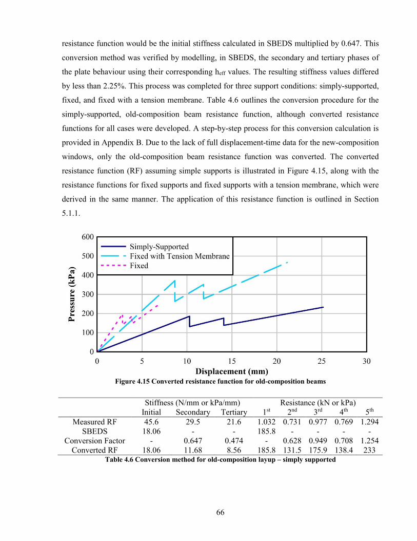
66

resistance function would be the initial stiffness calculated in SBEDS multiplied by 0.647. This

conversion method was verified by modelling, in SBEDS, the secondary and tertiary phases of

the plate behaviour using their corresponding heff values. The resulting stiffness values differed

by less than 2.25%. This process was completed for three support conditions: simply-supported,

fixed, and fixed with a tension membrane. Table 4.6 outlines the conversion procedure for the

simply-supported, old-composition beam resistance function, although converted resistance

functions for all cases were developed. A step-by-step process for this conversion calculation is

provided in Appendix B. Due to the lack of full displacement-time data for the new-composition

windows, only the old-composition beam resistance function was converted. The converted

resistance function (RF) assuming simple supports is illustrated in Figure 4.15, along with the

resistance functions for fixed supports and fixed supports with a tension membrane, which were

derived in the same manner. The application of this resistance function is outlined in Section

5.1.1.

Figure 4.15 Converted resistance function for old-composition beams

Stiffness (N/mm or kPa/mm) Resistance (kN or kPa) Initial Secondary Tertiary 1st 2nd 3rd 4th 5th

Measured RF 45.6 29.5 21.6 1.032 0.731 0.977 0.769 1.294 SBEDS 18.06 - - 185.8 - - - -

Conversion Factor - 0.647 0.474 - 0.628 0.949 0.708 1.254 Converted RF 18.06 11.68 8.56 185.8 131.5 175.9 138.4 233

Table 4.6 Conversion method for old-composition layup – simply supported

67

4.7 Limitations and Sources of Error A major limitation of the laboratory testing was the beam support conditions. In the field,

the laminated glass windows were attached to steel frames using structural silicone. In the

laboratory, the laminated glass beams were supported by pin and roller supports. The pin and

roller supports used in the laboratory did not allow membrane forces to develop in the glass or

interlayer. Furthermore, from Galuppi and Royer-Carfagni (2014), the Ψ value for a fixed beam

under a uniformly distributed load is 42/L2, 4.25 times larger than the value corresponding to a

simply-supported beam under the same load (9.88/L2). While the silicone supports used in the

field do not represent full fixity, they do allow a tension membrane to develop, which would

ultimately change the behaviour of the composition.

Another limitation is that the behaviour of PVB is highly temperature and load-duration

dependent. Both parameters affect the shear modulus of the interlayer, which is the main factor

in determining the amount of composite behaviour between the glass layers. The field tests and

laboratory tests were conducted at different temperatures and load durations, as outlined in

Table 4.7. Test data from Brackin (2010) is listed in Table 4.8 for temperature and load-duration

values similar to those in Table 4.7. It can be seen that the shear modulus value corresponding to

the field test parameters is a magnitude larger than the value corresponding to the laboratory test

parameters. In actuality, the shear modulus value for the field testing would be even higher, due

to the very short load duration, which is not reflected in Brackin’s work. To account for the

effect of temperature and load duration on the shear modulus of PVB, designers normally

assume that laminated glass acts monolithically in the pre-crack phase (Cormie et al., 2009,

Ledbetter et al., 2006), an assumption that will be examined in the next section.

Temperature (qC) Load Duration (s) Field Testing 12 to 14 ≈ 0.01

Laboratory Testing 26 ≈ 300 Table 4.7 Temperature and load duration comparison

Temperature (qC) Load Duration (s) Shear Modulus (MPa) 15.56 10 7.31 28.3 300 0.412

Table 4.8 Shear modulus values based on temperature and load duration (Brackin, 2010)

Despite the differences in both support conditions and shear modulus, the purpose of this

testing was to determine how well the measured resistance function from the laboratory tests,

68

once converted, was able to predict the behaviour of the multi-layered laminated glass window

systems when used in a SDOF analysis, which will be discussed in Section 5.1.1.

Finally, the stroke of the universal testing machine limited the displacement range over

which the beams were tested. Thus, the maximum resistance of the composite beam was never

reached.

4.8 Discussion Force-displacement curves for both the old- and new-composition beams were successfully

measured. Due to the consistency of data, a total of five beams was adequate to describe the

resistance function for each composition type. The new-composition beams, made with heat-

strengthened glass, showed a notable increase in strength over the old-composition beams, made

from annealed glass. However, these stronger new-composition beams also exhibited a

substantially reduced stiffness when compared to the old-composition beams, potentially due to

differing manufacturing processes. The method introduced by Galuppi and Royer-Carfagni

(2014) was used to determine the degree of monolithic behaviour of the old- and new-

composition beams, which was 0.623 and 0.447, respectively. Strain data was used to

corroborate that neither composition acted perfectly monolithically. The shear modulus for each

beam was calculated and showed reasonable correlation with values found in the literature.

Finally, the effective thickness of the laminated glass beam, which relates the tested beam to a

beam constructed solely of glass, was used, along with the program SBEDS, to convert the

measured force-displacement beam response to a pressure-displacement resistance function.

In future tests, it is recommended that the support conditions in the field be replicated in the

laboratory. This could be done by creating small C-channels out of steel plates, with the same

cross-sectional dimensions as the frames used in the field tests. Then, the beams could be

attached to the C-channels with structural silicone. This would allow a tension membrane to

develop in both the glass and interlayer, better representing the behaviour in the field. It would

also be valuable to test the beams in a machine that allowed for greater midspan displacement,

which would facilitate the measurement of maximum resistance. Ideally, the test should

terminate when the specimen has failed and not when the testing machine has run out of

displacement stroke. Furthermore, it would be useful to condition the beams at different

temperatures and test under different loading rates in order to observe the effect these variables

have on multi-layered laminated beams. Then, the behaviour of multi-layered laminated beams

at different temperatures and rates could be compared to that of simple laminated glass beams at

69

similar temperatures and rates to draw comparisons between their behaviours. Finally, strain

gauges could be adhered to the top and bottom faces of all glass and polycarbonate layers prior

to lamination, as done by Hooper (1973), which would facilitate an accurate measurement of the

strain, and therefore stress, distribution across the thickness of the composite.

70

5 Software Models Engineers rely heavily on software packages to determine the behaviour of glazing systems

subjected to blast loading. Little work has been done to verify the accuracy of these programs

when applied to multi-layered laminated glass. This chapter aims to compare the outputs from

several of these programs to the data collected from field blast tests. The main point of

comparison is between the measured displacement-time histories and those calculated by the

programs. Based on these comparisons, the reliability and accuracy of each program will be

assessed. More information on the individual blast analysis programs, namely SBEDS,

WINGARD, and CWBlast, can be found in Section 2.8.

5.1 Modelling Methodologies

5.1.1 SBEDS Modelling The version of SBEDS used in this research does not have a specific glazing option.

Instead, a combination of the two-way metal plate template and general SDOF template was

used. Two main cases with different resistance functions were investigated: (1) a plate modelled

using the converted resistance function from Section 4.6 and (2) a plate modelled assuming the

pre-cracked resistance function was equal to that of a monolithic plate. Each case was further

examined with both simply-supported and fixed boundary conditions. In addition, the fixed case

was analyzed both with and without a tension membrane (TM). For Case 1, the converted

resistance function was input into the general SDOF template, shown below in Figure 5.1. For

Case 2, the metal plate template, shown above in Figure 4.14, was used to determine the pre-

crack resistance function for a plate using an equivalent monolithic thickness of 34.9 mm. All

other inputs, except density, which was altered to achieve the correct mass, were identical to

those found in Figure 4.14. The geometric and material inputs are then used by SBEDS to create

a resistance function. Once the pre-crack portion of the resistance function was determined (i.e.

the first linear portion of the resistance function calculated by SBEDS), the method outlined in

Section 4.6 and Table 4.6 was used to extend the monolithic resistance function, using the ratios

measured in the laboratory. The complete calculation method can be seen in Appendix C. The

resulting resistance function for simply-supported boundary conditions is illustrated in Figure

5.2, along with the corresponding converted resistance function from the laboratory tests for

comparison. The pressure-time histories from Test 1 and Test 2 were input directly into SBEDS.

71

Figure 5.1 SBEDS general SDOF inputs – extended monolithic resistance function – simply supported

Figure 5.2 SBEDS resistance functions – simply supported

5.1.2 WINGARD Modelling As outlined in Section 2.8.2, WINGARD is straightforward to use. The user simply selects

materials from an existing database and creates the window layup to be analyzed. Alternatively,

72

the user can input their own materials with custom material properties. For the current research,

analyses were run using both the default WINGARD material properties and nominal properties

from the literature, as no material testing was completed. In practice, designers normally use

nominal values, and thus one would expect that WINGARD would output displacement-time

histories that are roughly accurate, even if the inputs are not exact. The material properties used

in the WINGARD analyses are summarized in Table 5.1, Table 5.2, and Table 5.3. A nominal

static strength of 80 MPa was chosen for annealed glass, which was increased by a DIF of 1.15,

based on the empirical relationships determined by Zhang et al. (2012), to generate a dynamic

strength of 92 MPa. However, WINGARD does not use a DIF to determine the dynamic

strength of materials; instead, a probability of failure is input for both the static and dynamic

conditions. Thus, the probability of failure was manipulated in order to achieve a dynamic

strength of 92 MPa for the annealed glass. The material properties for Marlon FSX (Brett Martin

Ltd., 2015), the polycarbonate used in the windows, were used as the nominal properties, which

matched closely to the defaults found in WINGARD. Regarding the PVB interlayer, the

datasheet for Butacite (Kuraray, 2015) was consulted and used as the base material properties,

as this material was used in the field-tested windows. Research from Brackin (2010) and Zhang

et al. (2015a), as well as data released from DuPont in 2004 (Brackin, 2010), was used to vary

the Young’s modulus of the PVB based on temperature and load duration. These values range

from 7.32 MPa to 344.7 MPa. This was done to see if WINGARD predictions were improved

when taking these factors into account, as they are known to influence the shear modulus, and

thus the Young’s modulus of polyvinyl butyral. Also, it is unclear how the default material

properties for PVB were chosen. A total of 6 analyses were completed in WINGARD for both

specimen O-T1-S2 (Test 1) and O-T2-S1 (Test 2). The three layup materials, namely annealed

glass, polycarbonate, and PVB, had their properties varied as outlined in Table 5.4.

Young’s Modulus (MPa)

Poisson’s Ratio Static Stress (kPa)

Dynamic Stress (kPa)

WINGARD 68,947.6 0.22 27,579 100,728.6 Nominal 70,000 0.22 80,000 92,000

Table 5.1 Annealed glass material properties

Young’s Modulus (MPa)

Poisson’s Ratio Yield Stress (kPa)

WINGARD 2,378.69 0.38 65,500 Nominal 2,350 0.38 60,000

Table 5.2 Polycarbonate material properties

73

Young’s Modulus (MPa)

Poisson’s Ratio

Tensile Strength (kPa)

Elongation at break

Elastic* 344.7 0.5 24,131.6 0 Elastic-Plastic* 344.7 0.5 20,684.3 2.05

Butacite (Kuraray, 2015) 7.32 0.5 28,144.4 2.75 Brackin, 2010 21.95 0.5 28,144.4 2.75 DuPont, 2004 24.18 0.5 28,144.4 2.75

Zhang et al, 2015a 36.5 0.5 28,144.4 2.75 Table 5.3 PVB material properties (* values are WINGARD defaults)

Case Annealed Glass Polycarbonate PVB 1 WINGARD Default Elastic 2 WINGARD Default Elastic-Plastic 3 Nominal Nominal Butacite 4 Nominal Nominal Brackin, 2010 5 Nominal Nominal DuPont, 2004 6 Nominal Nominal Zhang et al, 2015

Table 5.4 Analyses completed in WINGARD for each specimen

All of the windows were analysed using the reflected pressure-time history measured in the

field. In addition, the wet-glazing option in WINGARD was utilized. Dow Corning 121

structural silicone (Dow Corning, 2015) was used in the field-blasted windows, with a bite of 50

mm, a bead thickness of 11.5 mm and a strength of approximately 2.4 MPa. These wet-glazing

parameters were input into the program.

5.1.3 CWBlast Modelling Much like WINGARD, CWBlast contains a material library, and the user can use

predefined material properties or create their own custom materials. As CWBlast only models

the system behaviour up to first cracking, the first step was to determine whether changing the

PVB properties had any effect on this portion of the behaviour. Preliminary analyses indicated

that changing the PVB parameters had no effect on the pre-crack displacement behaviour. This

suggests that CWBlast assumes the amount of shear transfer between glass layers is the same

regardless of the Young’s modulus for the interlayer. Therefore, only two layup cases were

modelled in CWBlast, as listed in Table 5.5. Each of the listed models was run as both a simply-

supported plate and a fixed plate, due to the assumption that the structural silicone support

condition falls somewhere in between these two cases. Users are able to define elastic supports

in CWBlast; however, this option was not used as the stiffness of the structural silicone was not

measured.

74

Annealed Glass PVB Polycarbonate 1 CWBlast CWBlast Nominal 2 Nominal Butacite Nominal

Table 5.5 Analysis completed in CWBlast for each specimen

CWBlast allows designers to use different failure criteria to determine the behaviour of

laminated glass, namely the maximum principal stress (MPS) method and the glass failure

prediction method (GFPM) model. Due to the absence of material testing, only the MPS method

was used in this analysis.

Finally, unlike SBEDS and WINGARD, where the measured pressure-time histories were

directly used, CWBlast requires the peak pressure and impulse to be input, from which a linear

equivalent load is developed. The pressure equivalent used to model Test 1 is shown below in

Figure 5.3, indicating that the loading methods match closely. It must be noted that this loading

method ignores the negative phase. However, in the field tests, the peak inbound displacement

was reached before the negative phase commenced, which excludes the negative phase

behaviour from the comparison.

Figure 5.3 CWBlast linear equivalent pressure-time history – Test 1

5.2 Comparison of Model Output to Experimental Data

5.2.1 SBEDS In order to understand the SBEDS results below, the following items must be noted. In the

laboratory tests, the resistance function was only measured until the maximum stroke of the

universal testing machine was reached. Thus, the maximum resistance of the beam was not

measured. When using the general SDOF template in SBEDS, the resistance function does not

75

terminate at the last resistance point. Instead, the program assumes that the resistance keeps

increasing based on the last stiffness value that was input. Because of this, the results from

SBEDS are split into two segments. The solid line indicates the behaviour that corresponds with

the measured resistance function, whereas the dashed line represents the behaviour past this

point, where SBEDS continued to increase the resistance based on the last input stiffness value.

Therefore, the dashed lines indicate the predicted behaviour of the system, assuming the

resistance function continues indefinitely. In addition, the displacement-time behaviour for all

cases continued to oscillate past the cut-off point depicted in the figures below. However, the

damping of the system is unknown, and as such, any data past the first peak is not included in

the results. As previously mentioned, damping is generally ignored in blast loading, as it has

little influence on the first peak displacement, which is the parameter of interest in this

comparison.

Figure 5.4 shows the Test 1 comparison for Case 1, which used the converted resistance

function from the laboratory tests, with Table 5.6 listing the key values. Neither the shape nor

maximum displacement values for either the simply-supported or fixed plate matched the

measured field data. An observable mismatch in the time of peak displacement can be seen,

suggesting there is a discrepancy between the period of vibration of the measured and predicted

responses. The period of vibration, T, is influenced by the mass and stiffness of a system, and is

calculated as follows:

𝑇 = 2𝜋√𝑚𝑘

(5.1)

In Figure 5.4, it is clear that SBEDS underestimated the period when compared to the measured

data, meaning that the stiffness of the resistance function in SBEDS was too high or the mass of

the system was too low. The mass, however, was a fairly known quantity, as it can be calculated

based on the geometry of the individual layers and their associated densities. Therefore, in order

to achieve better period matching, the stiffness of the system must be adjusted.

76

Figure 5.4 Case 1 SBEDS comparison – Test 1

Maximum Displacement

(mm)

Time of Maximum Displacement

(ms) Simply-Supported (SS) 52.9 6.82

Fixed with Tension Membrane (TM) 24.7 4.74 Fixed 18.88 3.92

Measured 35.3 7.69 Table 5.6 Case 1 SBEDS important values – Test 1

Figure 5.5 Case 1 stiffness modifications – Test 1

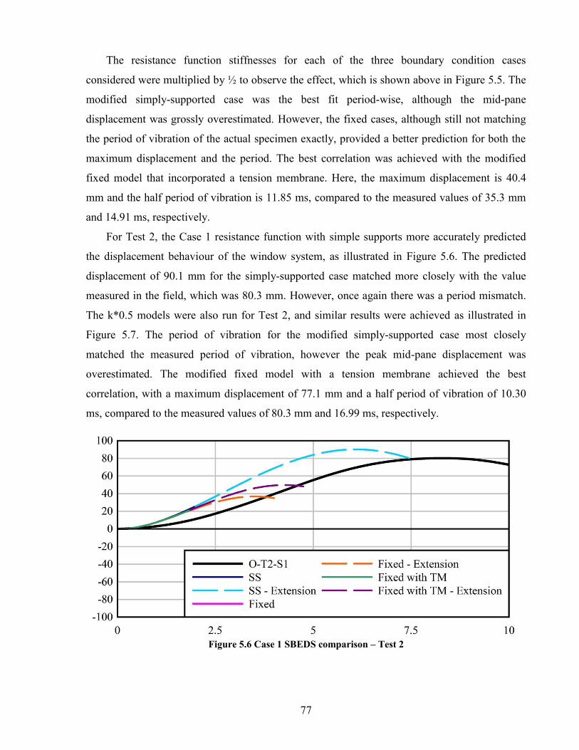
77

The resistance function stiffnesses for each of the three boundary condition cases

considered were multiplied by ½ to observe the effect, which is shown above in Figure 5.5. The

modified simply-supported case was the best fit period-wise, although the mid-pane

displacement was grossly overestimated. However, the fixed cases, although still not matching

the period of vibration of the actual specimen exactly, provided a better prediction for both the

maximum displacement and the period. The best correlation was achieved with the modified

fixed model that incorporated a tension membrane. Here, the maximum displacement is 40.4

mm and the half period of vibration is 11.85 ms, compared to the measured values of 35.3 mm

and 14.91 ms, respectively.

For Test 2, the Case 1 resistance function with simple supports more accurately predicted

the displacement behaviour of the window system, as illustrated in Figure 5.6. The predicted

displacement of 90.1 mm for the simply-supported case matched more closely with the value

measured in the field, which was 80.3 mm. However, once again there was a period mismatch.

The k*0.5 models were also run for Test 2, and similar results were achieved as illustrated in

Figure 5.7. The period of vibration for the modified simply-supported case most closely

matched the measured period of vibration, however the peak mid-pane displacement was

overestimated. The modified fixed model with a tension membrane achieved the best

correlation, with a maximum displacement of 77.1 mm and a half period of vibration of 10.30

ms, compared to the measured values of 80.3 mm and 16.99 ms, respectively.

Figure 5.6 Case 1 SBEDS comparison – Test 2

78

Figure 5.7 Case 1 stiffness modifications - Test 2

The predicted displacement-time histories produced from Case 2, which used the

assumption that laminated glass acts monolithically before it cracks, did not relate well to the

field measured data from Test 1 in terms of peak displacement. The peak displacement was

severely underestimated, as shown in Figure 5.8. However, the initial rate of displacement for

all three cases correlated well with the measured data. The initial measured rate of displacement

was approximately 3.40 mm/s, while the simply-supported case and fixed case had rates of

displacement of 4.08 mm/s and 2.95 mm/s, respectively. Similar results for Case 2 were

obtained with Test 2 data. This suggests that the monolithic assumption may be valid for multi-

layered laminated glass in the pre-crack phase. However, further examination is required as the

time of first cracking was not recorded in the field tests, and, as such, the duration of the pre-

crack phase cannot be explicitly defined.

Promising results were obtained when considering the slope of the displacement-time

history. A line was fitted to the linear portion of the inbound displacement prediction for Test 1,

based on the Case 1 fixed condition results (i.e. the laboratory-measured resistance function).

This was compared to the displacement-time history collected for O-T1-S2, as shown in Figure

5.9. Here, it is clear that, while both displacement and period predictions were inaccurate (see

Figure 5.4), the inbound slopes of the displacement-time histories correlated well.

79

Figure 5.8 Case 2 SBEDS comparison – Test 1

Figure 5.9 Lab RF fit with test 1 data

Thus, the traditional assumption of monolithic behaviour under blast loading may apply to

the initial response of a multi-layered laminated glass window under blast loading, however the

results achieved using the converted resistance function from the laboratory test better predict

the mid-pane displacement and stiffness of the system. Overall, it is postulated that an even

better correlation could be achieved with further refinements to the resistance function.

5.2.2 WINGARD In general, there was very poor correlation between the WINGARD output and the data

collected in the field tests. Regardless of the material properties used, every analysis grossly

overestimated the mid-pane deflection. WINGARD also overestimated the amount of damage

80

the windows sustained, always reporting that more components failed than what was observed

in the field. Thus, the program appears to be overly conservative for these types of window

compositions.

Figure 5.10 shows the comparison between the measured displacement-time history from

specimen O-T1-S2 (Test 1) and the six different WINGARD models, while Table 5.7

summarizes the outputs from each model. None of the models did a good job predicting the

displacement behaviour of the window system. The lowest predicted mid-pane displacement,

116 mm from the elastic-plastic PVB model in WINGARD, was still 3.3 times larger than the

measured central pane displacement of 35 mm. Additionally, it was observed in the field that

only layers G2, G3, and G4 cracked, whereas WINGARD predicted, at a minimum, that all

glass layers failed (Case 6) and, at a maximum, that all layers, including the PVB and

polycarbonate, failed (Case 2). WINGARD also predicted that the window attachment, or

structural silicone, failed for Cases 3 through 5, while no failure was evident in the field-tested

specimens. However, as noted in the analysis text output file created by WINGARD, the current

analysis procedure for wet-glazed systems (i.e. a window system using structural silicone) is

only preliminary and has not been tested or validated significantly by the developers of the

software.

One observation made from Figure 5.10 is that by increasing the Young’s modulus of the

interlayer, the mid-pane displacement decreases. Referring to Table 5.3, the Young’s modulus

for Butacite is the lowest, at 7.32 MPa, while the default Young’s modulus for both the elastic

and elastic-plastic PVB is approximately 345 MPa. This result makes sense, as an increase in

Young’s modulus would increase the shear modulus, which would in turn increase the stiffness

of the composite, due to an increase in composite behaviour.

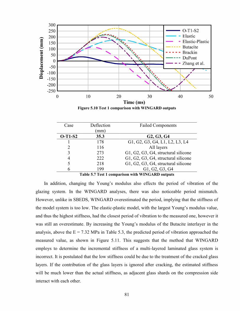
81

Figure 5.10 Test 1 comparison with WINGARD outputs

Case Deflection (mm)

Failed Components

O-T1-S2 35.3 G2, G3, G4 1 178 G1, G2, G3, G4, L1, L2, L3, L4 2 116 All layers 3 273 G1, G2, G3, G4, structural silicone 4 222 G1, G2, G3, G4, structural silicone 5 218 G1, G2, G3, G4, structural silicone 6 199 G1, G2, G3, G4

Table 5.7 Test 1 comparison with WINGARD outputs

In addition, changing the Young’s modulus also effects the period of vibration of the

glazing system. In the WINGARD analyses, there was also noticeable period mismatch.

However, unlike in SBEDS, WINGARD overestimated the period, implying that the stiffness of

the model system is too low. The elastic-plastic model, with the largest Young’s modulus value,

and thus the highest stiffness, had the closest period of vibration to the measured one, however it

was still an overestimate. By increasing the Young’s modulus of the Butacite interlayer in the

analysis, above the E = 7.32 MPa in Table 5.3, the predicted period of vibration approached the

measured value, as shown in Figure 5.11. This suggests that the method that WINGARD

employs to determine the incremental stiffness of a multi-layered laminated glass system is

incorrect. It is postulated that the low stiffness could be due to the treatment of the cracked glass

layers. If the contribution of the glass layers is ignored after cracking, the estimated stiffness

will be much lower than the actual stiffness, as adjacent glass shards on the compression side

interact with each other.

82

Figure 5.11 Young's modulus sensitivity study in WINGARD

Similar observations were made for specimen O-T2-S1 (Test 2), which are summarized in

Figure 5.12 and Table 5.8. Once again, the mid-pane displacements and reported levels of

damage from WINGARD vastly overestimated the behaviour observed in the field tests. Here,

all of the modelled windows either completely failed or came unattached from the frame, when,

in reality, the field-tested specimen remained in its frame with damage only visible in the glass

layers.

Figure 5.12 Test 2 comparison with WINGARD outputs

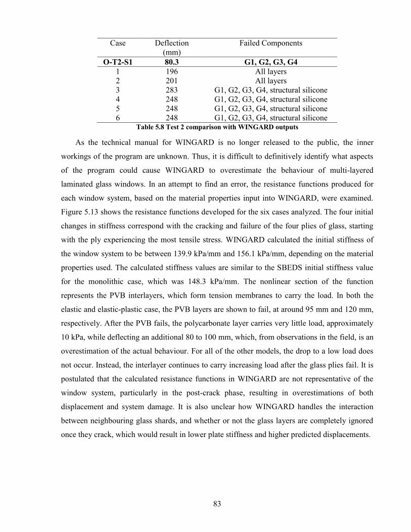
83

Case Deflection (mm)

Failed Components

O-T2-S1 80.3 G1, G2, G3, G4 1 196 All layers 2 201 All layers 3 283 G1, G2, G3, G4, structural silicone 4 248 G1, G2, G3, G4, structural silicone 5 248 G1, G2, G3, G4, structural silicone 6 248 G1, G2, G3, G4, structural silicone

Table 5.8 Test 2 comparison with WINGARD outputs

As the technical manual for WINGARD is no longer released to the public, the inner

workings of the program are unknown. Thus, it is difficult to definitively identify what aspects

of the program could cause WINGARD to overestimate the behaviour of multi-layered

laminated glass windows. In an attempt to find an error, the resistance functions produced for

each window system, based on the material properties input into WINGARD, were examined.

Figure 5.13 shows the resistance functions developed for the six cases analyzed. The four initial

changes in stiffness correspond with the cracking and failure of the four plies of glass, starting

with the ply experiencing the most tensile stress. WINGARD calculated the initial stiffness of

the window system to be between 139.9 kPa/mm and 156.1 kPa/mm, depending on the material

properties used. The calculated stiffness values are similar to the SBEDS initial stiffness value

for the monolithic case, which was 148.3 kPa/mm. The nonlinear section of the function

represents the PVB interlayers, which form tension membranes to carry the load. In both the

elastic and elastic-plastic case, the PVB layers are shown to fail, at around 95 mm and 120 mm,

respectively. After the PVB fails, the polycarbonate layer carries very little load, approximately

10 kPa, while deflecting an additional 80 to 100 mm, which, from observations in the field, is an

overestimation of the actual behaviour. For all of the other models, the drop to a low load does

not occur. Instead, the interlayer continues to carry increasing load after the glass plies fail. It is

postulated that the calculated resistance functions in WINGARD are not representative of the

window system, particularly in the post-crack phase, resulting in overestimations of both

displacement and system damage. It is also unclear how WINGARD handles the interaction

between neighbouring glass shards, and whether or not the glass layers are completely ignored

once they crack, which would result in lower plate stiffness and higher predicted displacements.

84

Figure 5.13 WINGARD old-composition resistance functions

5.2.3 CWBlast The current version of CWBlast calculates window response up until first cracking. Thus,

when using the program for laminated glass, the post-crack behaviour is not modelled. The post-

crack behaviour is equally as important as the pre-crack behaviour, and thus, CWBlast has a

very limited use for laminated glass systems.

Therefore, the uncracked behaviour predicted by CWBlast was compared to the

displacement-time history collected in the field. As seen in Figure 5.14, the difference between

material properties in Case 1 (i.e. the default CWBlast properties) and Case 2 (i.e. the nominal

values) did not alter the shape of the predicted displacement-time histories. Case 2 properties

resulted in a slightly higher displacement at failure, but the difference is negligible. Thus, it was

deemed unnecessary to model further cases.

Neither the simply-supported (SS) nor fixed boundary condition models match the field data

closely. The rate of increase of the displacement for both boundary conditions was much greater

than that observed in the field.

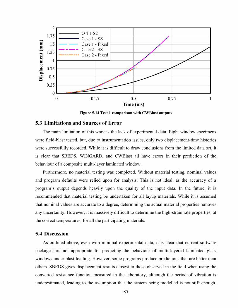
85

Figure 5.14 Test 1 comparison with CWBlast outputs

5.3 Limitations and Sources of Error The main limitation of this work is the lack of experimental data. Eight window specimens

were field-blast tested, but, due to instrumentation issues, only two displacement-time histories

were successfully recorded. While it is difficult to draw conclusions from the limited data set, it

is clear that SBEDS, WINGARD, and CWBlast all have errors in their prediction of the

behaviour of a composite multi-layer laminated window.

Furthermore, no material testing was completed. Without material testing, nominal values

and program defaults were relied upon for analysis. This is not ideal, as the accuracy of a

program’s output depends heavily upon the quality of the input data. In the future, it is

recommended that material testing be undertaken for all layup materials. While it is assumed

that nominal values are accurate to a degree, determining the actual material properties removes

any uncertainty. However, it is massively difficult to determine the high-strain rate properties, at

the correct temperatures, for all the participating materials.

5.4 Discussion As outlined above, even with minimal experimental data, it is clear that current software

packages are not appropriate for predicting the behaviour of multi-layered laminated glass

windows under blast loading. However, some programs produce predictions that are better than

others. SBEDS gives displacement results closest to those observed in the field when using the

converted resistance function measured in the laboratory, although the period of vibration is

underestimated, leading to the assumption that the system being modelled is not stiff enough.

86

However, the program is the most customizable, as the user is able to input their own resistance

function. With further refinements to the resistance function, it is foreseeable that SBEDS could

accurately predict the behaviour of complex window systems. The difficulty here is obtaining

the correct resistance function. In the future, it would be valuable to determine the load-

displacement behaviour of a composite window under uniform pressure with supports matching

the field conditions, which could then be compared to the converted resistance function, helping

to validate the methodology used in this research.

In current practice, WINGARD, while overestimating the behaviour, would likely be the

most suitable option for design, based on the software programs examined. Due to its

conservative predictions, window systems would be overdesigned and safe. However, work

needs to be done to determine the flaws in its calculation process, as overdesign is costly.

Finally, the applicability of CWBlast, in its current form, is low when considering multi-

layered laminated glass windows. As CWBlast does not predict the behaviour past first

cracking, the program is unable to predict the peak inbound displacement and total system

damage, two parameters that are very important when dealing with laminated glass windows.

87

6 Conclusions and Recommendations Full-scale field blast tests were conducted on two unique window compositions in order to

collect experimental data on the behaviour of multi-layered laminated glass windows under blast

loading. Sufficient pressure, displacement, and strain data were collected for both tests to

facilitate software validation, despite the fact that many instrumentation failures occurred. In

addition, the window compositions were qualitatively compared, and results showed that the

different compositions performed better at different scaled distances. Both window systems,

however, generated little debris in the test cubicle after testing, demonstrating the protective

nature of multi-layered laminated glass window systems.

Further laboratory testing was completed to better understand the behaviour of the

composite, as well as determine a static resistance function for use in SDOF analysis. Multi-

layered laminated glass beams constructed from the same material as the field-blasted

specimens were tested statically under four-point bending with pin and roller supports. Both

compositions acted neither monolithically nor layered: their behaviour was between the two

bounding cases. The effective thickness of the laminated glass beam, which relates the tested

beam to a beam constructed solely of glass, was used, along with the program SBEDS, to

convert the measured force-displacement beam response to a pressure-displacement resistance

function with three distinct boundary conditions: simply-supported, fixed, and fixed with a

tension membrane.

Finally, the experimental data was compared to the output of three predictive software

programs: SBEDS, WINGARD, and CWBlast. The main point of comparison between the field-

measured data and the software output was the displacement-time history, which involved

comparing the first peak mid-pane displacement and the period of vibration. The predictive

capabilities of each program were found to be limited. None of the software packages were able

to accurately model the overall shape of the displacement-time history. Additionally, none were

able to predict the peak mid-pane displacement with much precision. SBEDS predictions, using

the resistance function measured in the laboratory, were the most accurate in terms of

displacement and overall rate of displacement. When a “monolithic glass window” resistance

function was used in SBEDS, only the initial (pre-cracking) rate of displacement correlated

well. When using either the laboratory resistance function or a monolithic glass resistance

function, SBEDS underestimated the period of response. Conversely, WINGARD overestimated

the period of response, as well as the mid-pane displacement and the damage experienced by the

88

window, regardless of the materials used. Finally, CWBlast, which only models the pre-crack

phase, highly overestimated the initial rate of displacement.

Recommendations can be put forth for the applicability of each program, based on the

above discussion of their accuracy:

x SBEDS: Provided that the resistance function of the window system can be accurately

measured, SBEDS is the preferred blast program. However, obtaining the resistance

function may be difficult, as temperature and load duration influence the behaviour of

the composite.

x WINGARD: While overestimating the response, it is a conservative (i.e. safe) choice

for design. One major downside to WINGARD, though, is the lack of available

information about the methodology behind the program, making it difficult to adjust

inputs in order to receive more precise outputs.

x CWBlast: In its current form, it does not have the capability to predict the post-crack

behaviour of laminated glass and, thus, is not recommended for this application.

There is ample opportunity to conduct further research into multi-layered laminated glass

windows, whether under static or dynamic loading. Beam tests with different loading,

temperature, and boundary conditions could be conducted to ascertain the effects of these

parameters on the degree of composite behaviour exhibited. Similar tests could be conducted on

multi-layered laminated glass plates. In order to extend the blast loading research, further field

blast tests are required, and the suggested instrumentation improvements should be adopted to

ensure the collection of usable data. Once the material properties are measured, additional

modelling using, for example, finite element analysis should be undertaken to better understand

the behaviour of this complex composite system under static and dynamic loading conditions.

89

7 References Amstock, J.S. (1997). Handbook of Glass in Construction. New York, USA: McGraw Hill.

ARA. (2010a). WINGARD PE (Version 6.0). Albuquerque, USA: Applied Research Associates,

Inc.

ARA. (2010b). WINGARD PE 6.0 User Guide. Albuquerque, USA: Applied Research

Associates, Inc.

ASTM. (2012a). ASTM C1048-12 Standard Specification for Heat-Strengthened and Fully

Tempered Flat Glass. West Conshohocken, USA: ASTM International.

ASTM. (2012b). ASTM F1642-12 Standard Test Method for Glazing and Glazing Systems

Subject to Airblast Loadings. West Conshohocken, USA: ASTM International.

Autodesk. (2015). AutoCAD 2015. San Rafael, USA: Autodesk, Inc.

Baker, W.E. (1973). Explosions in Air. Austin, USA: University of Texas Press.

Beer, F.P., Johnston Jr, E.R., Dewolf, J.T., Mazurek, D.F. (2009). Mechanics of Materials (5th

Edition). New York, USA: McGraw-Hill.

Behr, R.A., Minor, J.E., Linden, M.P., Vallabhan, C.V.G. (1985). Laminated Glass Units Under

Uniform Lateral Pressure. Journal of Structural Engineering, 111(5), 1037-1050.

Behr, R.A., Minor, J.E., Norville, H.S. (1993). Structural Behaviour of Architectural Laminated

Glass. Journal of Structural Engineering, 119(1), 202-222.

Bennison, S.J., Jagota, A., Smith, C.A. (1999). Fracture of Glass/Poly(vinyl butyral) (Butacite®)

Laminates in Biaxial Flexure. Journal of the American Ceramic Society, 82(7), 1761-1770.

Biggs, J.M. (1964). Introduction to Structural Dynamics. New York, USA: McGraw-Hill.

90

Bottenbruch, L. (1996). Polycarbonates, Polyacetals, Polyesters, Cellulose Esters: Engineering

Thermoplastics. Munich, Germany: Carl Hanser Verlag.

Bougard, A. (2003). An Alternative Explosive for Full-Scale Glazing Tests. Proceedings of the

11th International Symposium on Interaction of the Effects of Munitions with Structures.

Mannheim, Germany, Proceedings on CD.

Brackin, M.S. (2010). Development of a Procedure to Evaluate the Shear Modulus of Laminated

Glass Interlayers (Master’s Thesis). Texas, USA: Texas A&M University.

Brett Martin Ltd. (2015). Marlon FSX Factsheet. Newtownabbey, UK: Brett Martin Ltd.

BSI. (2001a). BS EN 13123-1:2001 Windows, doors and shutters. Explosion resistance.

Requirements and classification. Shock tube. London, UK: BSI British Standards.

BSI. (2001b). BS EN 13124-1:2001 Windows, doors and shutters. Explosion resistance. Test

method. Shock tube. London, UK: BSI British Standards

BSI. (2004a). BS EN 13123-2:2004 Windows, doors, and shutters. Explosion resistance.

Requirements and classification. Range test. London, UK: BSI British Standards.

BSI. (2004b). BS EN 13124-2:2004 Windows, doors and shutters. Explosion resistance. Test

method. Range test. London, UK: BSI British Standards.

Cormie, D., Mays, G., Smith, P. (2009). Blast Effects on Buildings (2nd edition). London, UK:

Thomas Telford Limited.

DA. (1965). Fundamentals of Protective Design (Non-nuclear). TM 5-855-1. Washington, DC,

USA: Department of the Army.

DoD. (2008). Structures to Resist the Effects of Accidental Explosions. UFC 3-340-02.

Washington, DC, USA: Department of Defense.

91

Dow Corning. (2015). Dow Corning 121 Structural Glazing Sealant. USA: Dow Corning.

Du Bois, P.A., Kolling, S., Fassnacht, W. (2003). Modelling of Safety Glass for Crash

Simulation. Computational Materials Science, 28, 675-683.

Fischer, K., Häring, I. (2009). SDOF Response Model Parameters from Dynamic Blast Loading

Experiments. Engineering Structures, 31, 1677-1686.

Folgar, F. (2005). Advanced Aliphatic Polyurethane Resins for High Durability and Superior

Ballistic Performance Laminated Glass. Proceedings of the 22nd International Symposium on

Ballistics. Vancouver, Canada, 908-916.

Galuppi, L., Royer-Carfagni, G. (2012a). Effective Thickness of Laminated Glass Beams: New

Expression via a Variational Approach. Engineering Structures, 38, 53-67.

Galuppi, L., Royer-Carfagni, G. (2012b). The Effective Thickness of Laminated Glass Plates.

Journal of Mechanics of Materials and Structures, 7, 375-400.

Galuppi, L., Royer-Carfagni, G. (2014). Enhanced Effective Thickness of Multi-Layered

Laminated Glass. Composites: Part B, 64, 202-213.

Gardon, R. (1985). Strong Glass. Journal of Non-Crystalline Solids, 73, 233-246.

Griffith, A.A. (1921). The Phenomena of Rupture and Flow in Solids. Philosophical

Transactions of the Royal Society of London, 221, 163-198.

GSA. (2003). TS01 – 2003 Standard Test Method for Glazing and Window Systems Subject to

Dynamic Overpressure Loadings. Washington, USA: General Services Administration.

Holmquist, T.J., Johnson, G.R., Grady, D.E., Lopatin, C.M., Hertel Jr., E.S. (1995). High Strain

Rate Properties and Constitutive Modeling of Glass. Proceedings of the 15th International

Symposium on Ballistics. Jerusalem, Israel, 237-244.

92

Hooper, J.A. (1973). On the Bending of Architectural Laminated Glass. International Journal of

Mechanical Sciences, 15, 309-323.

Hooper, P.A., Blackman, B.R.K., Dear, J.P. (2012a). The Mechanical Behaviour of Poly(vinyl

butyral) at Different Strain Magnitudes and Strain Rates. Journal of Materials Science, 47(8),

3564-3576.

Hooper, P.A., Sukhram, R.A.M., Blackman, B.R.K., Dear, J.P. (2012b). On the Blast Resistance

of Laminated Glass. International Journal of Solids and Structures, 49(6), 899-918.

HydeSoft Computing. (2014). DPlot (Version 2.3.3.8). Vicksburg, USA: HydeSoft Computing.

Irwin, G.R. (1957). Analysis of Stresses and Strains Near the End of a Crack Traversing a Plate.

Journal of Applied Mechanics, 24(1), 361-364.

ISO. (2007a). ISO 16933:2007 Glass in Building – Explosion-Resistant Security Glazing – Test

and Classification for Arena Air-Blast Loading. Geneva, Switzerland: ISO.

ISO. (2007b). ISO 16934:2007 Glass in Building – Explosion-Resistant Security Glazing – Test

and Classification for Shock-Tube Loading. Geneva, Switzerland: ISO.

Khorasani, N. (2004). Design Principles for Glass Used Structurally: Rapport TABK-04/1025.

Lund: Lunds University Department of Building Science.

Kolsky, H. (1949). An Investigation of the Mechanical Properties of Materials at Very High

Rates of Loading. Proceedings of the Physical Society Section B, 62(11), 676-700.

Krauthammer, T., Altenberg, A. (2000). Negative Phase Blast Effects on Glass Panels.

International Journal of Impact Engineering, 24, 1-17.

Krynski, M. (2008). Dynamic Response of Architectural Glazing Subject to Blast Loading

(MASc Thesis). Toronto, Canada: University of Toronto.

93

Kuraray. (2015). Butacite PVB Properties. Houston, USA: Kuraray Americas, Inc.

Ledbetter, S., Walker, A., Keiller, A. (2006). Structural Use of Glass. ASCE Journal of

Architectural Engineering, 12(3), 137-149.

LeGrand, D.G., Bendler, J.T. (2000). Handbook of Polycarbonate Science and Technology.

New York, USA: Marcel Decker, Inc.

Megson, T.H.G. (2014). Structural and Stress Analysis (3rd edition). New York, USA: Elsevier

Science Publishing Company.

Menčík, J. (1992). Strength and Fracture of Glass and Ceramics. New York, USA: Elsevier

Science Publishing Company.

Moore, D.M. (1980). Proposed Method for Determining the Glass Thickness of Rectangular

Glass Solar Collector Panels Subjected to Uniform Normal Pressure Loads. Pasadena, USA: Jet

Propulsion Laboratory.

Morison, C. M. (2006). Dynamic Response of Walls and Slabs by Single-Degree-of-Freedom

Analysis – A Critical Review and Revision. International Journal of Impact Engineering, 32,

1214-1247.

Morison, C. (2007). The Resistance of Laminated Glass to Blast Pressure Loading and the

Coefficients for Single Degree of Freedom Analysis of Laminated Glass (PhD Thesis).

Cranfield, UK: Cranfield University.

Nicholas, T. (1980). Tensile Testing of Materials at High Rates of Strain. Experimental

Mechanics, 177-185.

Ngo, T., Mendis P., Gupta A., Ramsey, J. (2007). Blast Loading and Blast Effects on Structures

– An Overview. Electronic Journal of Structural Engineering (Special Issue: Loading on

Structures), 76-91.

94

Norville, H.S., King, K.W., Swofford, J.L. (1998). Behaviour and Strength of Laminated Glass.

Journal of Engineering Mechanics, 124(1), 46-53.

Patterson, M. (2011). Structural Glass Facades and Enclosures. Hoboken, USA: John Wiley &

Sons.

Pelfrene, J., Kuntsche, J., Van Dam, S., Van Paepegem, W., Schneider, J. (2016). Critical

Assessment of the Post-Breakage Performance of Blast Loaded Laminated Glazing:

Experiments and Simulations. International Journal of Impact Engineering, 88, 61-71.

Peroni, M., Solomos, G., Pizzinato, V., Larcher, M. (2011). Experimental Investigation of High

Strain-Rate Behaviour of Glass. Applied Mechanics and Materials, 82, 63-68.

Polcyn, M.A., Myers, K.D. (2010). Use of SBEDS for Blast Resistant Design in accordance

with UFC 3-340-02. San Antonio, USA: Baker Engineering and Risk Consultants.

Ritchie, C., Packer, J.A., Seica, M., Yankelevsky, D. (2014). Field Blast Testing and SDOF

Analysis of Unfilled and Concrete-Filled RHS Members. Proceedings of the 23rd International

Symposium on Military Aspects of Blast and Shock (MABS 23). Oxford, United Kingdom,

Paper no. 31.

Scholze, H. (1991). Glass: Nature, Structure, and Properties. New York, USA: Springer-Verlag.

Seica, M.V., Krynski, M., Walker, M., Packer, J.A. (2011). Analysis of Dynamic Response of

Architectural Glazing Subject to Blast Loading. Journal of Architectural Engineering, 17(2), 59-

74.

Spiller, K., Packer, J.A., Seica, M.V., Yankelevsky, D.Z. (2016). Prediction of Annealed Glass

Window Response to Blast Loading. International Journal of Impact Engineering, 88, 189-200.

Szilard, R. (2004). Theories and Applications of Plate Analysis – Classical, Numerical and

Engineering Methods. Hoboken, USA: John Wiley & Sons.

95

Ugural, A.C. (2009). Stresses in Beams, Plates, and Shells. Boca Raton, USA: Taylor & Francis

Group.

USACE. (1957). Design of Structures to Resist the Effects of Atomic Weapons – Principles of

Dynamics Analysis and Design. EM 1110-345-415. Washington, DC, USA: U.S. Army Corps

of Engineers.

USACE. (2008). Methodology Manual for the Single-Degree-of-Freedom Blast Effects Design

Spreadsheet (SBEDS). U.S. Army Corps of Engineers.

USACE. (2009). Single-Degree-of-Freedom Blast Effects Design Spreadsheet (SBEDS)

(Version 4.1). U.S. Army Corps of Engineers.

Vallabhan, C.V.G., Das, Y.C., Kamineni, S. (1990). Nonlinear Dynamic Response of Window

Glass Units. Journal of Wind Engineering and Industrial Aerodynamics, 36, 1155-1162.

Vallabhan, C.V.G., Das, Y C., Magdi, M., Asik, M., Bailey, J.R. (1993). Analysis of Laminated

Glass Units. Journal of Structural Engineering, 119(5), 1572-1585.

Vallabhan, C. V. G., Das, Y. C., Ramasamudra, M. (1992). Properties of PVB Interlayer Used

in Laminated Glass. Journal of Materials in Civil Engineering, 4(1), 71-76.

Van Duser, A., Jagota, A., Bennison, S.J. (1999). Analysis of Glass/Polyvinyl Butyral

Laminates Subjected to Uniform Pressure. Journal of Engineering Mechanics, 125(4), 435-442.

Walker, M., Seica, M., Eytan, A., Packer, J.A. (2012). Standards and Strategies for Blast

Testing of Structures and Devices. Proceedings of the 22nd International Symposium on Military

Aspects of Blast and Shock (MABS 22). Bourges, France, Paper no. 64.

Wedding, C.W. (2010). Experimental Study of Blast Resistant Glazing System Response to

Explosive Loading (Master’s Thesis). Lexington, Kentucky: University of Kentucky.

Wu, G.P. (2003). Structural Performance of Multi-Layered Laminated Glass Plates (PhD

Thesis). Swansea, Wales: Swansea University.

96

Ykman, P.A. (1991). Recent Developments in Aliphatic Thermoplastic Polyurethanes.

Proceedings of Thermoplastic Elastomers III. Brussels, Belgium, 1-3.

Zhang, X., Hao, H., Shi, Y., Cui, J. (2015a). The Mechanical Properties of Polyvinyl Butyral

(PVB) at High Strain Rates. Construction and Building Materials, 93, 404-415.

Zhang, X., Hao, H., Wang, Z. (2015b). Experimental Study of Laminated Glass Window

Responses under Impulsive and Blast Loading. International Journal of Impact Engineering, 78,

1-19.

Zhang, X., Shi, Y., Hao, H., Cui, J. (2015c). The Mechanical Properties of Ionoplast Interlayer

Material at High Strain Rates. Materials & Design, 83, 387-399.

Zhang, X., Zou, Y., Hao, H., Li, X., Ma, G., Liu, K. (2012). Laboratory Test on Dynamic

Material Properties of Annealed Float Glass. International Journal of Protective Structures, 3(4),

407-430.

97

Appendices

A. Field Blast Test Data Test 1 Test 2

P (kPa) 497 1237 ta (ms) 19.62 11.63 t0 (ms) 9.70 7.45

b 0.884 2.40 I (kPa-ms) 1855 2385

Table A.1 Friedlander fit values

Figure A.1 Free-field pressure and impulse readings - Test 1

Figure A.2 Reflected pressure and impulse readings - Test 1

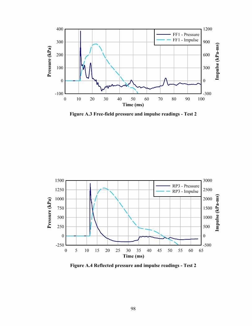
98

Figure A.3 Free-field pressure and impulse readings - Test 2

Figure A.4 Reflected pressure and impulse readings - Test 2

99

Figure A.5 Pane central displacement: O-T1-S2

Figure A.6 Pane central displacement: O-T2-S1

IN

OUT

IN OUT

100

Figure A.7 Period of oscillation: O-T1-S2

Figure A.8 Period of oscillation: O-T2-S1

62

73

82

94 IN OUT

IN OUT

114

144

101

Figure A.9 Pane central strain: O-T1-S1-H

Figure A.10 Pane central strain: O-T1-S1-V

102

Figure A.11 Pane central strain: O-T1-S2-H

Figure A.12 Pane central strain: O-T1-S2-V

103

Figure A.13 Pane central strain: N-T1-S1-H

Figure A.14 Pane central strain: N-T1-S1-V

104

Figure A.15 Pane central strain: N-T1-S2-H

Figure A.16 Pane central strain: N-T1-S2-V

105

Figure A.17 Pane central strain: O-T2-S1-H

Figure A.18 Pane central strain: O-T2-S1-V

106

Figure A.19 Pane central strain: O-T2-S2-H

Figure A.20 Pane central strain: O-T2-S2-V

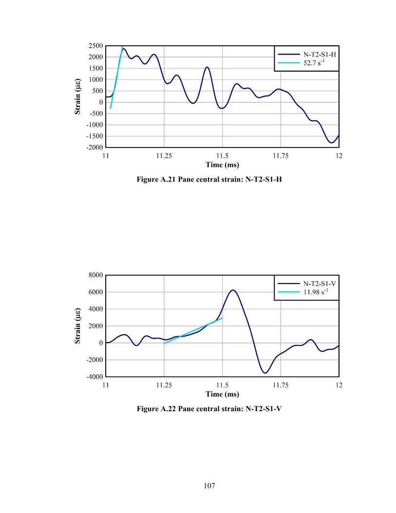
107

Figure A.21 Pane central strain: N-T2-S1-H

Figure A.22 Pane central strain: N-T2-S1-V

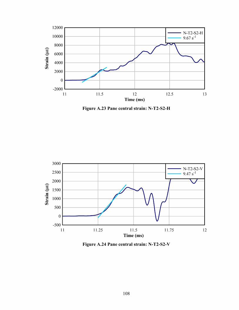
108

Figure A.23 Pane central strain: N-T2-S2-H

Figure A.24 Pane central strain: N-T2-S2-V

109

Figure A.25 Test specimen drawing - DYNA-01

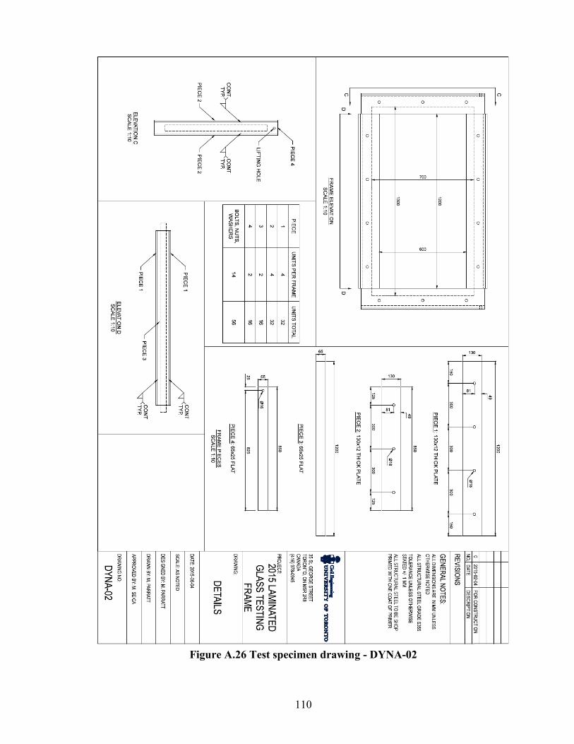
110

Figure A.26 Test specimen drawing - DYNA-02

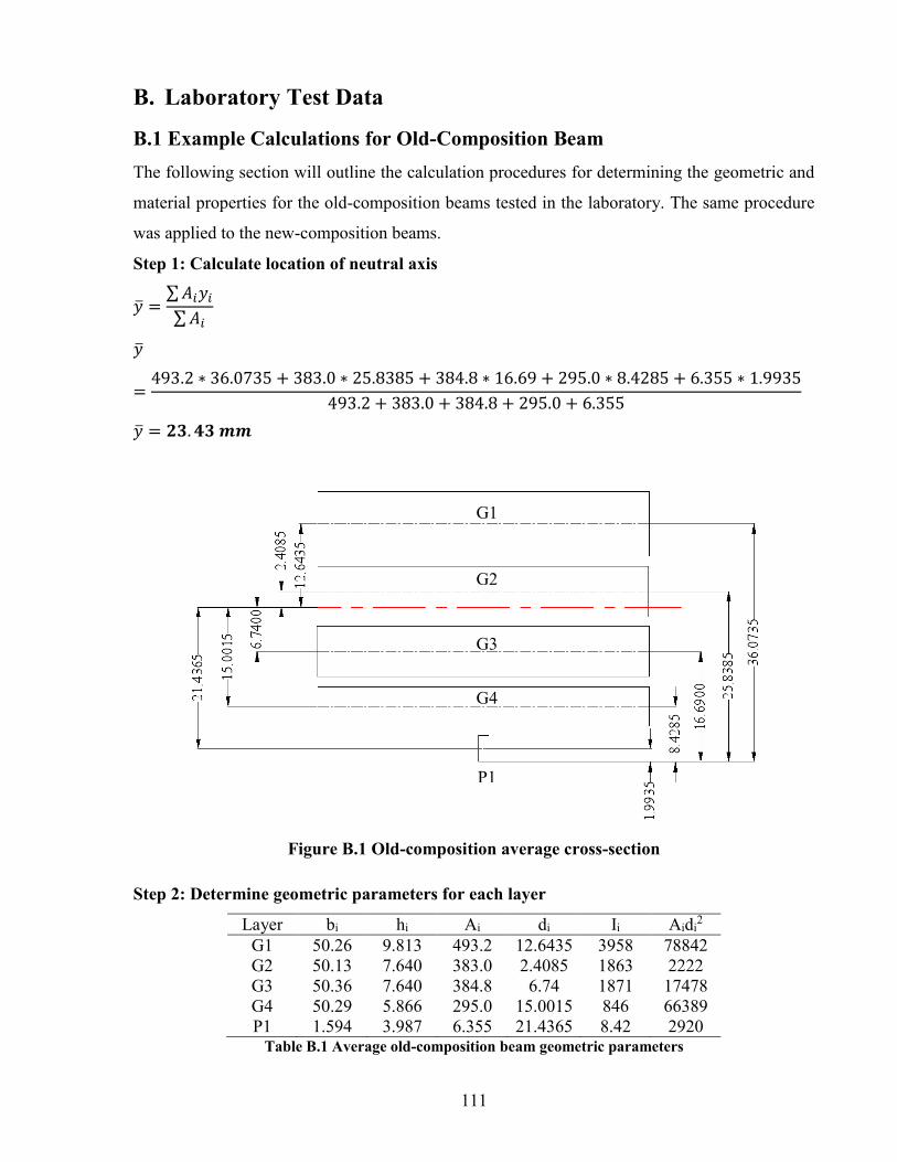
111

B. Laboratory Test Data

B.1 Example Calculations for Old-Composition Beam The following section will outline the calculation procedures for determining the geometric and

material properties for the old-composition beams tested in the laboratory. The same procedure

was applied to the new-composition beams.

Step 1: Calculate location of neutral axis

�̅� =∑ 𝐴𝑖𝑦𝑖

∑ 𝐴𝑖

�̅�

=493.2 ∗ 36.0735 + 383.0 ∗ 25.8385 + 384.8 ∗ 16.69 + 295.0 ∗ 8.4285 + 6.355 ∗ 1.9935

493.2 + 383.0 + 384.8 + 295.0 + 6.355

�̅� = 𝟐𝟑. 𝟒𝟑 𝒎𝒎

Figure B.1 Old-composition average cross-section

Step 2: Determine geometric parameters for each layer

Layer bi hi Ai di Ii Aidi2

G1 50.26 9.813 493.2 12.6435 3958 78842 G2 50.13 7.640 383.0 2.4085 1863 2222 G3 50.36 7.640 384.8 6.74 1871 17478 G4 50.29 5.866 295.0 15.0015 846 66389 P1 1.594 3.987 6.355 21.4365 8.42 2920

Table B.1 Average old-composition beam geometric parameters

G1

G2

G3

G4

P1

112

bi = average width of ith layer

hi = average thickness of ith layer

Ai = cross-sectional area of ith layer = bihi

di = distance between centroid of entire cross-section and centroid of ith layer

Ii = moment of inertia of ith layer = bihi3/12

Aidi2 = parallel axis theorem term for ith layer

Note: The P1 value for bi is scaled to account for the difference in Young’s modulus between

polycarbonate and glass (i.e. Epc/Eg = 2350/70000 = 0.0336)

Step 3: Calculate IL and IM

𝐼𝐿 = ∑ 𝐼𝑖 = 3958 + 1863 + 1871 + 846 + 8.42 = 𝟖𝟓𝟒𝟔 𝒎𝒎𝟒

𝐼𝑀 = ∑(𝐼𝑖 + 𝐴𝑖𝑑𝑖2)

= 3958 + 78842 + 1863 + 2222 + 1871 + 17478 + 846 + 66389 + 8.42 + 2920

= 𝟏𝟕𝟔𝟑𝟗𝟖 𝒎𝒎𝟒

Step 4: Calculate IR from experimental data

P/∆ = stiffness of beam = 45.6/2 = 22.8 N/mm

a = distance between support and adjacent loading point = 375 mm

E = Young’s modulus glass = 70,000 MPa

L = span of beam = 1,250 mm

𝐼𝑅 =𝑃∆

𝑎24𝐸

(3𝐿2 − 4𝑎2) = 22.8 ∗375

24 ∗ 70000(3 ∗ 12502 − 4 ∗ 3752) = 𝟐𝟎𝟗𝟗𝟑 𝒎𝒎𝟒

Step 5: Calculate n 1𝐼𝑅

=𝑛𝐼𝑀

+1 − 𝑛

𝐼𝐿

120993

=𝑛

176398+

1 − 𝑛8546

𝑛 = 𝟎. 𝟔𝟐𝟑

113

Step 6: Calculate hw and heff 1

(ℎ𝑤)3 =𝑛

∑ ℎ𝑖3 + 12 ∑ ℎ𝑖𝑑𝑖

2 +1 − 𝑛∑ ℎ𝑖

3

1(ℎ𝑤)3 =

0.6232102 + 12(5112)

+1 − 0.623

2102= 0.000189172

ℎ𝑤 = √0.000189172−13 = 𝟏𝟕. 𝟒𝟐 𝒎𝒎

ℎ𝑒𝑓𝑓 = √12𝐼𝑅

𝑏𝑎𝑣𝑔

3= √12 ∗ 20993

49.7043

= 𝟏𝟕. 𝟏𝟖 𝒎𝒎

bavg = average width of layers

Step 7: Solve for G

𝑛 =1

1 + 𝐸

𝐺𝑏𝑎𝑣𝑔𝐼𝑀 ∑ 𝐻𝑖2

𝑡𝑖

𝐼𝐿 ∑ 𝐴𝑖𝑑𝑖2 Ψ

Ψ = 10/L2 for simply-supported beam with point load

Ψ = 168/17L2 for simply-supported beam with uniformly distributed load

Hi = distance between centroids of adjacent glass layers i and i+1 = ℎ𝑖+ℎ𝑖+12

+ 𝑡𝑖

ti = thickness of ith interlayer layer = 1.5085 mm

Rearrange for G

𝐺 =𝐸𝐼𝐿 ∑(𝐴𝑖𝑑𝑖

2)Ψ

(1𝑛 − 1) 𝑏𝑎𝑣𝑔𝐼𝑀 ∑ 𝐻𝑖

2

𝑡𝑖

𝐺 =70000 ∗ 8546 ∗ 167851 ∗ Ψ

( 10.623 − 1) ∗ 49.704 ∗ 176398 ∗ 10.2352 + 9.14852 + 8.26152 + 6.4352

1.5085

𝐺 = 0.613 𝑀𝑃𝑎 for simply-supported beam with point load

𝐺 = 0.606 𝑀𝑃𝑎 for simply-supported beam with uniformly distributed load

𝐺𝑎𝑣𝑔 = 𝟎. 𝟔𝟎𝟗𝟓 𝑴𝑷𝒂

114

Table B.2 outlines the average dimensions for each layer in the new-composition beam. The

average depth was 41.03 mm.

Layer bi hi G1 50.23 5.866 G2 50.15 7.640 G3 50.42 7.640 G4 50.51 9.813 P1 1.595 3.987

Table B.2 Average new-composition beam geometric parameters

115

B.2 Example Calculations for Resistance Function Conversion The calculations below outline the procedure for converting the laboratory-measured beam

resistance functions into an equivalent resistance function for a plate for use in the program

SBEDS. This procedure is for the old-composition beam, assuming simple supports.

Step 1: Determine parameters from measured resistance function

Figure B.2 Old-composition beam resistance function

Force-Displacement Pairs Stiffnesses

A = 1031.879 N at 22.629 mm 1 = 45.6 N/mm

B = 731.012 N at 22.629 mm 2 = 29.5 N/mm

C = 976.9015 N at 30.964 mm 3 = 21.6 N/mm

D = 769.372 N at 30.964 mm

E = 1294.085 N at 55.256 mm

Step 2: Determine conversion factors

Forces Stiffnesses

B/A = 0.708 = F2 2/1 = 0.647 = S3

C/A = 0.947 = F3 3/1 = 0.474 = S5

D/A = 0.745 = F4

E/A = 1.254 = F5

116

Step 3: Determine first segment of resistance function in SBEDS

This step was achieved using the metal plate template in SBEDS. A plate was modelled with the

parameters listed below.

𝑡 =ℎ𝑤 + ℎ𝑒𝑓𝑓

2=

17.42 + 17.182

= 𝟏𝟕. 𝟑𝟎 𝒎𝒎

𝑤 = ∑(𝜌𝑖𝑣𝑖) = 𝜌𝑔𝑡𝑔 + 𝜌𝑝𝑣𝑏𝑡𝑝𝑣𝑏 + 𝜌𝑝𝑐𝑡𝑝𝑐

=(2,500 ∗ (9.813 + 7.64 + 7.64 + 5.866) + 1,066 ∗ 1.5085 ∗ 4 + 1,200 ∗ 3.987)

1000

= 𝟖𝟖. 𝟕 𝒌𝒈/𝒎𝟐

𝜌 =𝑤𝑡

=88.7

17.30 ∗ 0.001= 𝟓𝟏𝟐𝟓 𝒌𝒈/𝒎𝟑

Figure B.3 SBEDS metal plate input - simply-supported

The above inputs result in the following values for the first segment of the resistance function:

k1 = 18.06 kPa/mm

R1 = 185.8 kPa

x1 = 10.29 mm

117

Step 4: Convert resistance function

Using the ratios from Step 2, the first segment of the resistance function was extended, using the

following two equations:

𝑘𝑖 = 𝑆𝑖 ∗ 𝑘1

𝑅𝑖 = 𝐹𝑖 ∗ 𝑅1

Thus, the converted resistance function has the following parameters:

Stiffness Resistance

k1 = 18.06 kPa/mm R1 = 185.8 kPa

k2 = 0 kPa/mm R2 = 131.5 kPa

k3 = 11.68 kPa/mm R3 = 175.9 kPa

k4 = 0 kPa/mm R4 = 138.4 kPa

k5 = 8.56 kPa/mm R5 = 233 kPa

This resistance function was then input into the general-SDOF template in SBEDS to determine

the behaviour of the old-composition window system under blast loading.

118

B.3 Laboratory Test Data

Figure B.4 Beam O1 force-displacement curve

Figure B.5 Beam O2 force-displacement curve

119

Figure B.6 Beam O3 force-displacement curve

Figure B.7 Beam O4 force-displacement curve

120

Figure B.8 Beam O5 force-displacement curve

Figure B.9 Beam O6 force-displacement curve

121

Figure B.10 Beam N1 force-displacement curve

Figure B.11 Beam N2 force-displacement curve

122

Figure B.12 Beam N3 force-displacement curve

Figure B.13 Beam N4 force-displacement curve

123

Figure B.14 Beam N5 force-displacement curve

Figure B.15 Beam O1 strain data

124

Figure B.16 Beam O5 strain data

Figure B.17 Beam O6 strain data

125

Figure B.18 Beam N1 strain data

126

C. Software Programs

C.1 SBEDS Monolithic Resistance Function Conversion The following set of calculations outlines the procedure for determining the resistance function

for the window system assuming that the laminate acts 100% monolithically before cracking.

This procedure is for the old-composition beam, assuming simple supports.

Step 1: Determine first segment of the resistance function in SBEDS

This step was achieved using the metal plate template in SBEDS. A plate was modelled with the

parameters listed below.

𝑡 = √12 ∗ 𝑏

𝐼𝑀

3= √12 ∗ 49.704

1763983

= 𝟑𝟒. 𝟗 𝒎𝒎

𝑤 = ∑(𝜌𝑖𝑣𝑖) = 𝜌𝑔𝑡𝑔 + 𝜌𝑝𝑣𝑏𝑡𝑝𝑣𝑏 + 𝜌𝑝𝑐𝑡𝑝𝑐

=(2,500 ∗ (9.813 + 7.64 + 7.64 + 5.866) + 1,066 ∗ 1.5085 ∗ 4 + 1,200 ∗ 3.987)

1000

= 𝟖𝟖. 𝟕 𝒌𝒈/𝒎𝟐

𝜌 =𝑤𝑡

=88.7

34.9 ∗ 0.001= 𝟐𝟓𝟒𝟐 𝒌𝒈/𝒎𝟑

Figure C.1 SBEDS metal plate input - simply-supported

127

The above inputs result in the following values for the first segment of the resistance function:

k1 = 148.28 kPa/mm

R1 = 756.24 kPa

x1 = 5.10 mm

Step 4: Convert resistance function

Using the ratios from B.2 Step 2, the first segment of the resistance function was extended,

using the following two equations:

𝑘𝑖 = 𝑆𝑖 ∗ 𝑘1

𝑅𝑖 = 𝐹𝑖 ∗ 𝑅1

Thus, the converted resistance function has the following parameters:

Stiffness Resistance

k1 = 148.28 kPa/mm R1 = 756.24 kPa

k2 = 0 kPa/mm R2 = 535.42 kPa

k3 = 95.94 kPa/mm R3 = 716.16 kPa

k4 = 0 kPa/mm R4 = 561.89 kPa

k5 = 70.28 kPa/mm R5 = 948.32 kPa

This resistance function was then input into the general-SDOF template in SBEDS to determine

the behaviour of the old-composition window system under blast loading.

128

C.2 WINGARD Inputs

Figure C.2 Glass material property inputs for WINGARD

Figure C.3 Polycarbonate material property inputs for WINGARD

Figure C.4 Interlayer material property inputs for WINGARD

Figure C.5 Glass layup input in WINGARD, for Butacite interlayer

129

Figure C.6 Window system input for WINGARD, for Butacite interlayer