Behavioral Network Economics
223
Behavioral Network Economics Soham Phade Electrical Engineering and Computer Sciences University of California, Berkeley Technical Report No. UCB/EECS-2021-216 http://www2.eecs.berkeley.edu/Pubs/TechRpts/2021/EECS-2021-216.html September 14, 2021
Transcript of Behavioral Network Economics

Behavioral Network Economics
Soham Phade
Electrical Engineering and Computer SciencesUniversity of California, Berkeley
Technical Report No. UCB/EECS-2021-216
http://www2.eecs.berkeley.edu/Pubs/TechRpts/2021/EECS-2021-216.html
September 14, 2021

Copyright © 2021, by the author(s).All rights reserved.
Permission to make digital or hard copies of all or part of this work forpersonal or classroom use is granted without fee provided that copies arenot made or distributed for profit or commercial advantage and that copiesbear this notice and the full citation on the first page. To copy otherwise, torepublish, to post on servers or to redistribute to lists, requires prior specificpermission.
Acknowledgement
I would like to thank my advisor Venkat Anantharam and my other twocommittee members, Jean Walrand and David Aldous.

Behavioral Network Economics
by
Soham Rajesh Phade
A dissertation submitted in partial satisfaction of the
requirements for the degree of
Doctor of Philosophy
in
Engineering — Electrical Engineering and Computer Sciences
in the
Graduate Division
of the
University of California, Berkeley
Committee in charge:
Professor Venkat Anantharam, ChairProfessor Jean WalrandProfessor David Aldous
Summer 2021

Behavioral Network Economics
Copyright 2021by
Soham Rajesh Phade

1
Abstract
Behavioral Network Economics
by
Soham Rajesh Phade
Doctor of Philosophy in Engineering — Electrical Engineering and Computer Sciences
University of California, Berkeley
Professor Venkat Anantharam, Chair
Game theoretic models are prevalent in the study of interactions between autonomous agents.Given the pervasive role of humans as agents in networks (e.g. social networks) and markets(e.g. labor markets), building mechanisms based on presumably more accurate models ofhuman behavior is of great interest both for increasing human welfare and for buildingmore efficient commercial systems that interact with humans. Cumulative prospect theory(CPT), one of the leading models for decision-making under risk and uncertainty, introducedby Kahneman and Tversky, combines several psychological insights into decision theory.Theoretical economics has primarily focused on expected utility theory (EUT) to modelhuman behavior. On the other hand, CPT has been observed to be a better fit in empiricalstudies, it is a generalization of EUT, and has a nice mathematical formulation convenient fortheoretical studies. It provides a way to incorporate psychological aspects into the concreteframeworks of game theory and economics which is required in building large scale systemsthat are better aligned with human preferences and needs and are also robust to theiremotional traits. A systematic and principled approach is needed. This thesis aims to buildwork in this direction by studying the following three problems through the lens of CPT:
1. resource allocation over networks,
2. notions of equilibrium in non-cooperative games, and
3. mechanism design.
In this thesis, we develop theoretical tools and establish fundamental results that wouldsupport real-world applications and future research in behavioral network economics.

i
To Mummy and Dada.

ii
Contents
Contents ii
List of Figures v
List of Tables viii
1 Introduction 11.1 Motivation . . . . . . . . . . . . . . . . . . . . . . . . . . . . . . . . . . . . . 11.2 Examples and Applications . . . . . . . . . . . . . . . . . . . . . . . . . . . 31.3 The Tool: Cumulative Prospect Theory (CPT) . . . . . . . . . . . . . . . . . 71.4 Related Work and Overview . . . . . . . . . . . . . . . . . . . . . . . . . . . 13Appendix . . . . . . . . . . . . . . . . . . . . . . . . . . . . . . . . . . . . . . . 181.A Notational Conventions . . . . . . . . . . . . . . . . . . . . . . . . . . . . . . 18
2 Optimal Resource Allocation over Networks with CPT Players 202.1 Introduction . . . . . . . . . . . . . . . . . . . . . . . . . . . . . . . . . . . . 202.2 Lottery-Based Resource Allocation Model . . . . . . . . . . . . . . . . . . . 212.3 Discretization Trick . . . . . . . . . . . . . . . . . . . . . . . . . . . . . . . . 232.4 Pricing and Market-Based Mechanism . . . . . . . . . . . . . . . . . . . . . 252.5 A Quick Illustrative Example . . . . . . . . . . . . . . . . . . . . . . . . . . 292.6 Optimum Permutation Profile and Duality Gap . . . . . . . . . . . . . . . . 302.7 Average System Problem and Optimal Lottery Structure . . . . . . . . . . . 332.8 Summary . . . . . . . . . . . . . . . . . . . . . . . . . . . . . . . . . . . . . 36Appendix . . . . . . . . . . . . . . . . . . . . . . . . . . . . . . . . . . . . . . . 362.A Proof of Theorem 2.4.1 . . . . . . . . . . . . . . . . . . . . . . . . . . . . . . 372.B Proof of Lemma 2.6.1 . . . . . . . . . . . . . . . . . . . . . . . . . . . . . . . 382.C Proof of Proposition 2.6.2 . . . . . . . . . . . . . . . . . . . . . . . . . . . . 392.D Example to Show Duality Gap . . . . . . . . . . . . . . . . . . . . . . . . . . 402.E Proof of Theorem 2.6.3 . . . . . . . . . . . . . . . . . . . . . . . . . . . . . . 432.F Proof of Lemma 2.7.1 . . . . . . . . . . . . . . . . . . . . . . . . . . . . . . . 442.G Proof of Lemma 2.7.2 . . . . . . . . . . . . . . . . . . . . . . . . . . . . . . . 452.H Proof of Proposition 2.7.3 . . . . . . . . . . . . . . . . . . . . . . . . . . . . 47
iii
3 Notions of Equilibrium: CPT Nash Equilibrium and CPT CorrelatedEquilibrium 493.1 Introduction . . . . . . . . . . . . . . . . . . . . . . . . . . . . . . . . . . . . 493.2 Definitions . . . . . . . . . . . . . . . . . . . . . . . . . . . . . . . . . . . . . 503.3 Main Result: An Interesting Geometric Property . . . . . . . . . . . . . . . 523.4 Two by Two Games . . . . . . . . . . . . . . . . . . . . . . . . . . . . . . . 573.5 Connectedness . . . . . . . . . . . . . . . . . . . . . . . . . . . . . . . . . . . 643.6 Example of a Game with Disconnected CPT Correlated Equilibrium . . . . . 673.7 Summary . . . . . . . . . . . . . . . . . . . . . . . . . . . . . . . . . . . . . 69
4 Black-Box Equilibrium: Reconsidering CPT Nash Equilibrium 714.1 Introduction . . . . . . . . . . . . . . . . . . . . . . . . . . . . . . . . . . . . 714.2 CPT and Betweenness . . . . . . . . . . . . . . . . . . . . . . . . . . . . . . 734.3 Equilibrium in Black-Box Strategies . . . . . . . . . . . . . . . . . . . . . . . 774.4 Summary . . . . . . . . . . . . . . . . . . . . . . . . . . . . . . . . . . . . . 85Appendix . . . . . . . . . . . . . . . . . . . . . . . . . . . . . . . . . . . . . . . 874.A Proof of Theorem 4.2.3 . . . . . . . . . . . . . . . . . . . . . . . . . . . . . . 874.B An Interesting Functional Equation . . . . . . . . . . . . . . . . . . . . . . . 884.C Proof of Lemma 4.3.6 . . . . . . . . . . . . . . . . . . . . . . . . . . . . . . . 904.D Proof of Proposition 4.3.11 . . . . . . . . . . . . . . . . . . . . . . . . . . . . 904.E Proof of Theorem 4.3.12 . . . . . . . . . . . . . . . . . . . . . . . . . . . . . 904.F Joint Continuity of the Concave Hull of a Jointly Continuous Function . . . 92
5 Mediated Correlated Equilibrium: Reconsidering CPT Correlated Equi-librium 945.1 Introduction . . . . . . . . . . . . . . . . . . . . . . . . . . . . . . . . . . . . 945.2 Calibrated Learning in Games . . . . . . . . . . . . . . . . . . . . . . . . . . 965.3 Mediated Games and Equilibrium . . . . . . . . . . . . . . . . . . . . . . . . 1005.4 Calibrated Learning to Mediated CPT Correlated Equilibrium . . . . . . . . 1045.5 No-Regret Learning and CPT Correlated Equilibrium . . . . . . . . . . . . . 1065.6 Summary . . . . . . . . . . . . . . . . . . . . . . . . . . . . . . . . . . . . . 111Appendix . . . . . . . . . . . . . . . . . . . . . . . . . . . . . . . . . . . . . . . 1115.A Notions of equilibrium . . . . . . . . . . . . . . . . . . . . . . . . . . . . . . 1115.B Beyond Fixed Reference Points . . . . . . . . . . . . . . . . . . . . . . . . . 1135.C Generalized Signal Spaces . . . . . . . . . . . . . . . . . . . . . . . . . . . . 1165.D Proof of Lemma 5.3.3 . . . . . . . . . . . . . . . . . . . . . . . . . . . . . . . 1185.E Proof of Theorem 5.4.1 . . . . . . . . . . . . . . . . . . . . . . . . . . . . . . 1215.F Proof of Corollary 5.4.3 . . . . . . . . . . . . . . . . . . . . . . . . . . . . . . 1225.G Proof of Proposition 5.4.4 . . . . . . . . . . . . . . . . . . . . . . . . . . . . 1225.H Proof of Proposition 5.4.5 . . . . . . . . . . . . . . . . . . . . . . . . . . . . 1235.I Proof of proposition 5.5.1 . . . . . . . . . . . . . . . . . . . . . . . . . . . . 1275.J Proof of Lemma 5.5.4 . . . . . . . . . . . . . . . . . . . . . . . . . . . . . . . 128

iv
5.K Proof of Proposition 5.5.3 . . . . . . . . . . . . . . . . . . . . . . . . . . . . 128
6 Mediated Mechanism Design for CPT Players 1366.1 Introduction . . . . . . . . . . . . . . . . . . . . . . . . . . . . . . . . . . . . 1366.2 Mechanism Design Framework . . . . . . . . . . . . . . . . . . . . . . . . . . 1416.3 The Revelation Principle . . . . . . . . . . . . . . . . . . . . . . . . . . . . . 1486.4 Mediated Mechanisms and the Revelation Principle . . . . . . . . . . . . . . 1576.5 Summary . . . . . . . . . . . . . . . . . . . . . . . . . . . . . . . . . . . . . 169Appendix . . . . . . . . . . . . . . . . . . . . . . . . . . . . . . . . . . . . . . . 1726.A Proof of the Revelation Principle . . . . . . . . . . . . . . . . . . . . . . . . 1726.B Proof of Equation (6.A.6) . . . . . . . . . . . . . . . . . . . . . . . . . . . . 1806.C Outcome Sets can be Identified with the Allocation Set under EUT . . . . . 183
7 Concluding Remarks and Directions for Future Work 1877.1 Introduction . . . . . . . . . . . . . . . . . . . . . . . . . . . . . . . . . . . . 1877.2 Role of Communication, Data Analytics and Artificial Intelligence in Resource
Allocation . . . . . . . . . . . . . . . . . . . . . . . . . . . . . . . . . . . . . 1907.3 Fairness and Ethical Considerations . . . . . . . . . . . . . . . . . . . . . . . 1947.4 Conclusion . . . . . . . . . . . . . . . . . . . . . . . . . . . . . . . . . . . . . 196
Bibliography 197
Index 206

v
List of Figures
1.1 Allais Paradox: Lotteries involved in the thought experiments proposed by Allaisare shown. Each lottery is comprised of the winning amounts and the correspond-ing chance of winning these amounts. . . . . . . . . . . . . . . . . . . . . . . . . 8
1.2 Example of a typical value function. The plot shows value function v0 (i.e. ref-erence point r = 0) given in equation (1.3.5) with α1 = α2 = 0.5, and λ = 2.5.With reference point r = 0, positive outcomes (z > 0) are gains and negativeoutcomes (z < 0) are losses. The value at reference point r = 0 is 0. Notice thatthe value function is concave in the positive domain and convex in the negativedomain. Also, notice that value function is much more steeper in the negativedomain than in the positive domain giving rise to a kink at the origin. . . . . . 10
1.3 Example of a typical probability weighting function. The solid curve shows thetypical shape of a probability weighting function, be it for gains or for losses.The dotted line shows the identity function for reference. This marks the de-viation form EUT. Indeed, if the probability weighting function is given by theidentity function for both gains and losses, then the player has EUT preferenceswith the utility function given by the value function vr at its reference point.The plot shows the probability weighting function given by equation (1.3.6) withγ = 0.65. Notice that the probability weighting function is typically concaveinitially and convex later with an inflection point around 1/3. It over-weightssmaller probabilities and under-weights larger probabilities. The probabilisticsensitivity (derivative of the probability weighting function) is high near the endprobabilities, namely, 0 and 1, and low in the middle. . . . . . . . . . . . . . . . 11
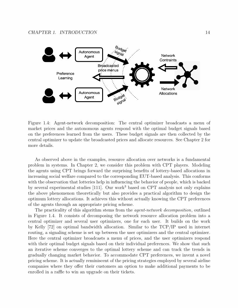
1.4 Agent-network decomposition: The central optimizer broadcasts a menu of mar-ket prices and the autonomous agents respond with the optimal budget signalsbased on the preferences learned from the users. These budget signals are thencollected by the central optimizer to update the broadcasted prices and allocateresources. See Chapter 2 for more details. . . . . . . . . . . . . . . . . . . . . . 14
1.5 Flow chart showing the dependence between different chapters and sections. . . 17
2.1 Probability weighting function for the example in Section 2.5. The plot showsthe probability weighting function given by equation (1.3.6) (also shown in Sec-tion 2.5) with γ = 0.61. The dotted line shows the identity function for reference. 29

vi
3.1 Payoff matrix (left) and joint probability matrix (right) of a 2× 2 game . . . . . 573.2 Canonical 2× 2 games . . . . . . . . . . . . . . . . . . . . . . . . . . . . . . . . 613.3 Vertices of the convex polytope CEUT for γI(α, β) . . . . . . . . . . . . . . . . . 623.4 The set CCPT for games of type (I) with weakly dominated strategies . . . . . . 633.5 The set CCPT for games of type (II) with weakly dominated strategies . . . . . . 643.1 Standard 2-simplex of probability vectors p = (pR, pY , pG). The shaded region
represents the set C(Γ, 1,TOP) and is disconnected. . . . . . . . . . . . . . . . . 693.2 Un-normalized distributions µ and µ. . . . . . . . . . . . . . . . . . . . . . . . . 70
4.1 The solid curve shows the probability weighting function for Alice from Exam-ple 4.2.1 and Example 4.3.7, and the dashed curve shows the probability weightingfunction for Charlie from Example 4.2.2. . . . . . . . . . . . . . . . . . . . . . . 75
4.1 Payoff matrix for Alice in Example 4.3.7. Rows and columns correspond to Alice’sand Bob’s actions respectively. The amount in each cell corresponds to Alice’spayoff. . . . . . . . . . . . . . . . . . . . . . . . . . . . . . . . . . . . . . . . . . 79
4.2 Payoff matrices for the 2× 2 game in Example 4.3.9 (left matrix for player 1 andright matrix for player 2). The rows and the columns correspond to the actionsof player 1 and player 2, respectively, and the entries in the cell represent thecorresponding payoffs. . . . . . . . . . . . . . . . . . . . . . . . . . . . . . . . . 80
4.3 The CPT value of player 1 in Example 4.3.9. Here, p and q denote the black-boxstrategies for player 1 and 2, respectively. Note the rise and sharp drop in thetwo curves near p = 1. For the curve for q = 0.3, the global maximum is attainedat p = 0, whereas, for the curve for q = 0.35, the global maximum is attainedclose to p = 1, specifically for some p ∈ [0.9, 1]. . . . . . . . . . . . . . . . . . . . 81
4.4 The figure (not to scale) shows the best response black-box strategy sets of thetwo players for the game in Example 4.3.9. The red (dashed) line shows the bestresponse black-box strategy set of player 2 in response to the black-box strategy(1 − p, p) of player 1. The green (solid) line shows the best response black-boxstrategy set of player 1 in response to the black-box strategy (1− q, q) of player2. Note that there is no intersection of these lines. . . . . . . . . . . . . . . . . . 82
4.5 Venn diagram depicting the different notions of equilibrium as subsets of theset S =
∏i ∆(Ai). The sets marked pNE,mNE,BBNE, and mBBNE represent
the sets of pure Nash equilibria, mixed action Nash equilibria, black-box strat-egy Nash equilibria, and mixed black-box strategy Nash equilibria, respectively.Examples are given in the body of the text of CPT games lying in each of theindicated regions (a) through (g). . . . . . . . . . . . . . . . . . . . . . . . . . 84
4.6 Payoff matrices for the 2×2 games in Example 4.3.15. The rows and the columnscorrespond to the actions of player 1 and player 2, respectively. In each cell, theleft and right entries correspond to player 1 and player 2, respectively. Thelabels indicate the corresponding regions in Figure 4.5. The game matrix for theexample corresponding to region (g) is the same as that for the one correspondingto region (a). . . . . . . . . . . . . . . . . . . . . . . . . . . . . . . . . . . . . . 86

vii
4.7 The CPT value function for player 1 in Example 4.3.15(b), when q = 0.5 is themixture of actions of player 2. . . . . . . . . . . . . . . . . . . . . . . . . . . . . 86
4.8 The CPT value function for player 1 in Example 4.3.15(e), when q = 0.5 is themixture of actions of player 2. . . . . . . . . . . . . . . . . . . . . . . . . . . . . 86
6.1 The solid curve shows the probability weighting function w+1 for player 1 from Ex-
ample 6.2.1 and Example 6.4.2. The dotted curve shows the probability weightingfunction w+
2 for player 2 in Example 6.2.1 and Example 6.4.2, which is the linearfunction corresponding to EUT preferences. . . . . . . . . . . . . . . . . . . . . 147
6.1 Probability weighting functions for the players in Example 6.3.1. . . . . . . . . . 1506.2 Plot of expression E(x) in Claim 6.3.2. . . . . . . . . . . . . . . . . . . . . . . . 1526.3 Plot of expression E1(z′) in Claim 6.3.3. . . . . . . . . . . . . . . . . . . . . . . 1536.4 Plot of expression E2(x′) in Claim 6.3.3. . . . . . . . . . . . . . . . . . . . . . . 1536.1 Plot of expression E3(x) in Example 6.4.3. . . . . . . . . . . . . . . . . . . . . . 166

viii
List of Tables
2.D.1Table showing the numerical evaluations corresponding to the example in Sec-tion 2.D. The numbers in the cells denote the optimum value of the objectivefunction (VIII) in the corresponding cases. . . . . . . . . . . . . . . . . . . . . . 42
3.1 Payoff matrix for the game in Section 3.6 . . . . . . . . . . . . . . . . . . . . . . 67
4.1 Different types of Nash equilibrium when players have CPT preferences. . . . . 87
5.1 Payoff matrix for the game Γ∗ in Example 5.2.1. The rows and columns cor-respond to player 1 and 2’s actions respectively. The first entry in each cellcorresponds to player 1’s payoff and second to player 2’s payoff. . . . . . . . . . 98
5.2 Empirical distribution µo for the action play in Example 5.2.1. . . . . . . . . . 995.3 Empirical distribution µe for the action play in Example 5.2.1. . . . . . . . . . 995.4 Empirical distribution µ∗ for the action play in Example 5.2.1. . . . . . . . . . . 995.K.1Empirical distribution µ in Example 5.5.2. . . . . . . . . . . . . . . . . . . . . . 131
6.1 Settings in which the revelation principle holds. . . . . . . . . . . . . . . . . . . 161

ix
Acknowledgments
Firstly, I would like to thank my advisor Venkat Anantharam. I am grateful to him forpointing me towards cumulative prospect theory (CPT), which has taken center stage inmy research and this thesis. His guidance has been pivotal in shaping my research. Oneof his amazing characteristics is that he is ultra-careful in everything he does, and that hasgreatly influenced my thinking, research, writing, and presentation. I am indebted to himfor his detailed feedback on all the documents and for all our discussions, full of originality,precision, witticism, and enlightening thoughts. I would also like to thank Jean Walrandand David Aldous for being a part of my dissertation committee, and Anant Sahai for beinga part of my qualifying exam committee. I am grateful to them for their helpful comments.
I thank my collaborators, Kannan Ramchandran, Thomas Courtade, Vipul Gupta, VidyaMuthukumar, and Anant Sahai. Conversations and correspondences with them have pro-vided me with the much-needed boost that makes research an exciting social engagement.I am grateful to the wonderful conferences as Allerton, GameNets, and Stony Brook GameTheory Center for providing me many more such opportunities with world-class researchers.I am thankful to Inderjit Dhillon for allowing me to intern at Amazon. I would also like tothank my fellow researchers at Amazon, Daniel Hill, Kedarnath Kolluri, Arya Mazumdar,Sujay Sanghvi, and Rajat Sen, for the illuminating discussions and for helping me under-stand the intricacies involved in implementing algorithms at such a large scale. I had theopportunity to teach as a graduate student instructor at UC Berkeley for EE226 with VenkatAnantharam and CS70 with Alistair Sinclair and Yun Song. Working with them has been agreat learning experience and has helped me improve my teaching and managerial skills. Iam grateful to them for giving me this opportunity. I am deeply indebted to Vivek Borkarfor advising me during my undergraduate studies and prodding me to join UC Berkeley. Hehas always been a great guide and a source of inspiration. I would also like to thank myIMO and IIT JEE coach, M. Prakash, who has advised me at every prime juncture of mycareer. One of the books that has helped me a lot during my PhD research is “ProspectTheory: For Risk And Ambiguity” by Peter Wakker, and I am grateful to him for writingthis valuable piece of work.
Secondly, I would like to thank my friends and colleagues at Berkeley who helped makethis journey memorable. BLISS lab has been an amazing place to be, full of intelligentpeople and exciting activities. I would like to thank Raaz Dwivedi, Sri Krishna Vadlamani,Sang Min Han, Kush Bhatia, Neha Gupta, Payam Delgosha, Vidya Muthukumar, AshwinPananjady, Orhan Ocal, Vijay Kamble, Varun Jog, Kangwook Lee, Nihar Shah, RashmiVinayak, Vasuki Narasimha Swamy, Fanny Yang, Yuting Wei, Dong Yin, Avishek Ghosh,Vipul Gupta, Aviva Bulow, Efe Aras, Kuan-Yun Lee, Vignesh Subramanian, Nived Ra-jaraman, Wenlong Mou, Banghua Zhou, Chinmay Maheshwari, Swanand Kadhe, AbishekSankararaman, Gireeja Ranade, Ramtin Pedarsani, Kabir Chandrashekher, Leah Dickstein,Tavor Baharav, Laura Brink, Aditya Ramdas, Reinhard Heckel, Ilan Shomorony, LudwigSchmidt, Koulik Khamaru, Milind Hegde, Anamika Chowdhury, Jimmy Narang, Nick Bhat-tacharya, Satyaki Mukherjee. In particular, thanks to Raaz and Sri Krishna for taking

x
this journey together. Thanks to Kush and Neha for being a part of my pandemic bubbleand helping me keep my sanity during these crazy times. I owe thanks to Shirley Salanio,Kim Kail, and Nicole Song for being extremely reliable and resourceful in resolving all myadministrative issues.
Finally, I would like to thank my parents – my mother Archana Phade, and my father,Rajesh Phade. Without their love and support none of this would have been possible, andthis thesis is dedicated to them.

1
Chapter 1
Introduction
1.1 Motivation
We will mainly be concerned with the study of social systems comprised of several individuals,typically humans, henceforth called players , interacting directly or indirectly in a boundedsituation (or an environment). Systems influenced by technological innovations over the pastseveral decades will be of particular interest to us. For example, these include transportationand communication networks, the Internet, computation networks and data-centers, energyand utility networks, financial networks, labor markets, social networks, and digital markets.
The complex nature of these systems requires consideration of several crucial aspectswhich gave rise to the interdisciplinary fields of cybernetics and systems science. Thesecombine knowledge from various fields such as control theory, information theory, dynamicalsystems, operations research, computer science, systems engineering, economics, statistics,and psychology. The engineering approach towards solving these problems primarily focuseson the physical aspects such as feasibility, practicality, maintainability, stability, and scal-ability. An equally important dimension is that of catering to individual preferences andneeds. Ultimately these systems are there for the users. Thus enters marketing researchand business management. These fields study the market economy and business processesto identify, anticipate and satisfy customers’ needs and wants. A holistic approach thatcombines these two approaches will go a long way.
Technological advancements in domains such as the Internet, Computing, Communica-tion, and Artificial Intelligence (AI) have lead to rapidly evolving network services such ascloud computing, smart information systems, multimedia platforms, software companies,online marketplaces, and smart grids, that have global scopes. Consequently, network eco-nomics research evolved along two major lines:
1. Optimal routing and control: This involved the study of flow dynamics and congestionbased on the underlying network structures and routing decisions. Typical problemsstudied include the shortest path problem, the maximum flow problem, the minimumcost flow problem, etc. (See books by Anna Nagurney [94, 95, 97, 98, 96].)

CHAPTER 1. INTRODUCTION 2
2. Network formation and growth: Here, the focus is on the understanding of the for-mation of network links, the flow of information in social networks or diseases in epi-demiological studies, connectivity and segregation in different networks, etc. Modelsfrom random graph theory and statistics are helpful in this approach. (See books byMathew Jackson [62, 63] and Sanjeev Goyal [54].)
Besides understanding the working of networks, a fundamental goal of network economicsis to assist decision-making for both the system designer and the players in the system. Forexample, Braess’ paradox warns a network planner of the following counter-intuitive effect:adding additional links to a network can reduce the overall system utility (such as the totaldelays for all the drivers in a transportation network) at Nash equilibrium when each player ismaking an optimal self-interested decision. Observations like these and results from networkeconomics have greatly helped policy-making and system design. (Shapiro and Varian [122]describe strategies to guide business decisions and policies in network economies such asdifferential pricing, utilizing network positive externalities and lock-in effects, patents andrights management, and others.)
Game theory and economics offer valuable guiding principles in the design of these sys-tems. The economic models for studying these problems typically assume that the partic-ipating agents are rational and possess immense computational power (which is reasonablewhen the participating agents are firms or nations). However, for e-commerce platforms likesocial media and online marketplaces, where the participating agents are single individualswho perform several repeated short-lived interactions with the platform, it is unusual thatthese agents would adhere to the above behavioral assumptions. We cannot expect thehuman mind to make informed and well-thought decisions in such complex interconnectedsystems, let alone the stress it generates. Our goal here is to use sophisticated models frombehavioral psychology and decision theory to model human interaction and design robustand scalable systems that would assist the users in making decisions that are in their owninterests and also for those around them.
The digital revolution has given rise to software companies having massive control overseveral crucial networks with the power to micromanage them. The algorithms deployedby these companies can influence social, economic, and political networks like never before.Along with all the evident benefits of these software systems in automating tasks and facil-itating large-scale network operations, we must pay closer attention to how these systemsinteract with their users. The growing human-computer interaction requires careful con-sideration of human behavior and their emotional responses. Our knowledge regarding theguiding principles for governing these interactions is quite limited, and a methodologicalapproach towards incorporating psychological aspects into system design is barely off theground. There is an ongoing debate relating to the benefits of these big technology com-panies, the extreme power these companies hold, and whether they are using it wisely ornot. Although it will not be the focus of this thesis, I hope that the behavioral foundationsdeveloped in this work would help answer some of these questions (see Section 7.3), andconsequently, help build systems that are better aware of human behavior and needs.
CHAPTER 1. INTRODUCTION 3
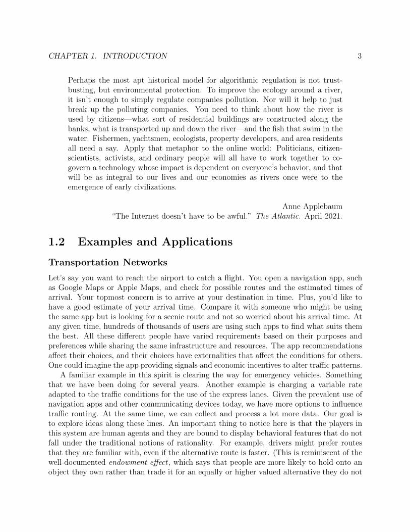
Perhaps the most apt historical model for algorithmic regulation is not trust-busting, but environmental protection. To improve the ecology around a river,it isn’t enough to simply regulate companies pollution. Nor will it help to justbreak up the polluting companies. You need to think about how the river isused by citizens—what sort of residential buildings are constructed along thebanks, what is transported up and down the river—and the fish that swim in thewater. Fishermen, yachtsmen, ecologists, property developers, and area residentsall need a say. Apply that metaphor to the online world: Politicians, citizen-scientists, activists, and ordinary people will all have to work together to co-govern a technology whose impact is dependent on everyone’s behavior, and thatwill be as integral to our lives and our economies as rivers once were to theemergence of early civilizations.
Anne Applebaum“The Internet doesn’t have to be awful.” The Atlantic. April 2021.
1.2 Examples and Applications
Transportation Networks
Let’s say you want to reach the airport to catch a flight. You open a navigation app, suchas Google Maps or Apple Maps, and check for possible routes and the estimated times ofarrival. Your topmost concern is to arrive at your destination in time. Plus, you’d like tohave a good estimate of your arrival time. Compare it with someone who might be usingthe same app but is looking for a scenic route and not so worried about his arrival time. Atany given time, hundreds of thousands of users are using such apps to find what suits themthe best. All these different people have varied requirements based on their purposes andpreferences while sharing the same infrastructure and resources. The app recommendationsaffect their choices, and their choices have externalities that affect the conditions for others.One could imagine the app providing signals and economic incentives to alter traffic patterns.
A familiar example in this spirit is clearing the way for emergency vehicles. Somethingthat we have been doing for several years. Another example is charging a variable rateadapted to the traffic conditions for the use of the express lanes. Given the prevalent use ofnavigation apps and other communicating devices today, we have more options to influencetraffic routing. At the same time, we can collect and process a lot more data. Our goal isto explore ideas along these lines. An important thing to notice here is that the players inthis system are human agents and they are bound to display behavioral features that do notfall under the traditional notions of rationality. For example, drivers might prefer routesthat they are familiar with, even if the alternative route is faster. (This is reminiscent of thewell-documented endowment effect , which says that people are more likely to hold onto anobject they own rather than trade it for an equally or higher valued alternative they do not

CHAPTER 1. INTRODUCTION 4
own. The fear of the unknown and uncertainty also plays a role here.) We must incorporatethese behavioral features into system modeling. Furthermore, this applies to all forms oftransportation services such as public transport, railways, airways, waterways, shipping ofgoods, etc.
Communication Networks
Using navigation apps to help route traffic is just an instance of taking advantage of theadvanced communication technologies for improving resource allocation. Indeed, communi-cating the availability of resources, individual preferences, and incentives for resource man-agement, and controlling system parameters require real-time information transfer and sig-naling. No wonder the Internet was the first to witness real-time algorithm-based trafficmanagement. Transmission Control Protocol (TCP) and bandwidth allocation algorithmshave helped avoid the congestion issues that had plagued the Internet before TCP. The the-oretical foundations for this work were laid by Kelly in the late 1990s [72, 73]. In Chapter 2,we extend these ideas to incorporate behavioral features and psychological traits displayedby the users.
Today, traffic shaping is a major area that deals with congestion control [84, 116]. Theusers are allocated bandwidth based on the choice of the monthly plans selected by themand the ambient network traffic conditions. One of our goals is to extend these ideas toreal-time traffic management. For example, imagine you have a virtual presentation comingup. It would be nice to indicate this to the service provider, such as Xfinity or AT&T, andrequest a boost for this period. It might result in additional charges, but it would provideyou the added benefit of choosing a more economical base plan. Certainly, re-engineeringthe Internet along these lines would increase user-system interactions and it would needalgorithms that are more aware of human behavior and responses.
Cloud Computing Networks
Just as communication networks allocate bandwidth to the users, cloud computing networks,such as Amazon Web Services, Microsoft Azure, or Google Cloud, provide on-demand com-puter system resources such as data storage and computing power. Cloud service providerscan schedule most of the customer jobs instantly today as the resources exceed the demand.However, with a growing trend of customers opting for computing resources as a serviceinstead of maintaining such systems on their own, this surplus luxury is not sustainable.Resources are also naturally constrained in settings such as fog computing and peer-to-peercomputing networks. Besides, concerns over the energy consumption by data centers isanother factor that limits the expansion of computing resources.
The demand for resources can vary significantly over time, different jobs have differentresource requirements, and customers have varying preferences towards their job delays andthe quality of service. The prices must conform to these changing demands in real-time.Although the typical customers in this setting are firms and organizations, the end-users

CHAPTER 1. INTRODUCTION 5
of their services and products are often individual humans. The value and revenue gener-ation for these organizations is closely related to the levels of consumer satisfaction. As aresult, behavioral considerations naturally creep into the utilities and preferences of theseorganizations.
Energy Networks
Smart grids are another excellent example of the application of digital processing and com-munications to systems where user interactions play a major role. The goal here is to improvethe economic efficiency of electricity networks and maintain high levels of quality of supplyby integrating the behavior and actions of all the users connected to the network - genera-tors, consumers, and those that do both. It would provide communication protocols to thesuppliers and the consumers, allowing them to be more flexible and sophisticated in theiroperational strategies. For example, the suppliers could indicate their energy prices, andthe consumers could indicate their willingness to pay in real-time. The users can configuresmart devices to generate additional energy or initiate energy-saving modes under specificsettings such as during high-cost peak usage periods. Similar to the pricing based on jobdelays in the cloud computing setting, we can imagine customers having different prefer-ences towards their energy requirements based on deadlines, for example, such requirementswould naturally occur in charging of electric vehicles. Today, PG&E, a utility company thatprovides natural gas and electric service, offers different pricing schemes such as time-of-userate plans and tiered usage rate plans. Along similar lines, we are interested in much moreflexible and sophisticated pricing schemes based on dynamic market conditions and humanbehavior analysis. This would also benefit in incentivizing people to shift to clean electricityoptions and adopt solar panels at home.
Social Networks
Several activities such as advertising, campaigning, or running welfare programs depend onthe underlying social networks. Humans are the primary agents in any social network. Theirinteractions and behavior form an integral part in the study of social networks. Models thatincorporate psychological aspects are needed to better allocate resources in these activities.It would help answer questions like: How can we maximize the impact of a campaign witha limited budget? How to best incentivize the agents in a network to perform actions thatare in the best interests of the entire society?
From a commercial point of view, it would greatly benefit the online ad exchange com-panies such as Google Ads or Facebook Ads. These are digital marketplaces that enableadvertisers to buy and sell advertising spaces. Here, user attention is the limited resourceand the different advertisers are competing for this limited resource. The tools developed inthis thesis will help regulate these markets more efficiently by incorporating human behav-ioral features.

CHAPTER 1. INTRODUCTION 6
Matching Markets
Just like the ad exchange marketplace, several other matching markets fall in this domain.These include labor markets that match employers and workers such as Upwork and Free-lancer, ride hailing applications that match drivers and riders such as Uber and Lyft, deliveryservices that match restaurants and diners such as Doordash and UberEats, or online mar-ketplaces that match sellers and buyers such as Amazon and eBay. Notice that most of theparticipating agents in these settings are individual humans susceptible to showing behaviorthat is influenced by biases and heuristics.
Finance and Insurance
Finance and insurance is another interesting setting where behavioral factors play a hugerole. There is a decent amount of work studying how individuals make decisions about theirinvestment strategies and insurance policies, but there is only a limited amount of work thatconsiders behavioral features in a financial network setting where the individuals interactwith each other and their decisions affect the other individuals in the network. In this work,we establish results that would facilitate this research.
Observe that, in all the above examples, the following factors are common:
1. The resources are limited.
2. Players have varying requirements and preferences.
3. The preferences of the players are private information.
4. Players have limited information about the system operations and constraints.
5. Players show behavioral features.
The goal is to design a communication protocol or a market system to fa-cilitate the exchange of information for strategic players who might displaybehavioral features, and consequently allocate resources to satisfy certain re-quirements. In contrast to prior works, we will pay special attention to the lastfactor, namely, the behavioral features of the players. We aim to bring these aspectsto the same level of mathematical sophistication as other aspects in system sciences. Suchan approach is crucial to building systems that are scalable across different users and robustto the intricacies of human behavior.
With me, everything turns intomathematics.
Rene Descartes

CHAPTER 1. INTRODUCTION 7
1.3 The Tool: Cumulative Prospect Theory (CPT)
Central to our approach is a mathematical model to capture human behavior and preferences.As is common in decision theory, we will consider the problem of decision-making by rationalagents under uncertainty. In many of the examples discussed above, the agents need to makedecisions without having complete information about the system and the behavior of otherplayers in the system. For instance, a person who is traveling needs to decide which routeto take without the exact information about traffic conditions, or a company launchinga new product needs to decide how to maximize its advertising impact without completeknowledge of its customers as well as its competitors. Decision-making under uncertaintyprovides a minimal framework that is general enough to capture the commonly encounteredinteractions, preferences, choices and actions of agents in a network.
Rationality is generally formulated as expected utility maximization. The justification forthis comes from the von Neumann and Morgenstern expected utility maximization theorem[130]. Although this assumption has a nice normative appeal to it and can be used to alarge extent as a prescriptive theory, it has been evident through several examples [3, 48,67] that the model is not that good an approximation for descriptive purposes. On theother hand, cumulative prospect theory (CPT) accommodates many empirically observedbehavioral features [127]. Proposed by Kahneman and Tversky, it is one of the leadingtheories for decision making under uncertainty. It has a nice mathematical formulation andis a generalization of expected utility theory (EUT).
A lottery (or prospect) is comprised of one or more outcomes with their correspondingprobabilities.1 We will denote a lottery by
L := (p1, z1), (p2, z2), . . . , (pt, zt), (1.3.1)
where zj ∈ R, 1 ≤ j ≤ t, denotes an outcome and pj, 1 ≤ j ≤ t, is the probability with whichoutcome zj occurs. We assume that the lottery is exhaustive, i.e.
∑tj=1 pj = 1. (Note that
we are allowed to have pj = 0 for some values of j and we can have zk = zl even when k 6= l.)Expected utility theory (EUT) posits that each individual is associated with a utility
function u : R→ R. The utility function is typically assumed to be concave (to capture therisk-averseness of the individual). The expected utility corresponding to lottery L is givenby
U(L) =t∑
j=1
pju(zj). (1.3.2)
A person is said to have EUT preferences if, given a choice between lottery L1 and lotteryL2, she chooses the one with the higher expected utility.
In the latter half of the 20th century, several people began documenting the limitations ofEUT to model human behavior. Allais paradox (1952) is a particularly interesting thoughtexperiment that marks the beginning of this work [3]. The experiment goes as follows:Consider the two lotteries shown in Experiment A of Figure 1.1. If you choose Lottery 1A,then you win $1 Million for sure, i.e. with a 100% chance. If you choose Lottery 2A, then

CHAPTER 1. INTRODUCTION 8
Experiment ALottery 1A Lottery 2A
Winning Chance Winning Chance$1 Million 100% $1 Million 89%
Nothing 1%$5 Million 10%
Experiment BLottery 1B Lottery 2B
Winning Chance Winning ChanceNothing 89% Nothing 90%
$1 Million 11%$5 Million 10%
Figure 1.1: Allais Paradox: Lotteries involved in the thought experiments proposed by Allaisare shown. Each lottery is comprised of the winning amounts and the corresponding chanceof winning these amounts.
you win $1 Million with a 89% chance, you do not win anything with a 1% chance, and youwin $5 Million with a 10% chance. You can choose only one of the two lotteries and it is aone time offer. Which one do you select? Now instead, consider Experiment B. The lotteriesare shown in Figure 1.1. Again you can choose only one of the two lotteries and it is a onetime offer. Which one now?
It is quite common for people to choose Lottery 1A in Experiment A and Lottery 2B inExperiment B. The paradox arises from the following observation: Lottery 1B is obtainedfrom Lottery 1A by transforming 89% chance of winning $1 Million to winning nothing. Theremaining 11% chance of winning $1 Million is left as is. When a similar transformation isapplied to Lottery 2A, we get Lottery 2B. Note that the 89% chance of winning $1 Millionin Lottery 2A changed to nothing combined with the 1% chance of winning nothing givesthe 90% chance of winning nothing in Lottery 2B. The 10% chance of winning $5 Millionremains unchanged.
The above observation underlies the fact that the choice of Lottery 1A and Lottery 2Bis inconsistent with EUT. To see this, let u be the utility function of the individual. Choiceof Lottery 1A over Lottery 2A implies
u($1M) > 0.89u($1M) + 0.01u($0) + 0.10u($5M). (1.3.3)
And choice of Lottery 2B over Lottery 1B implies
0.89u($0) + 0.11u($1M) > 0.90u($0) + 0.10u($1M). (1.3.4)
No utility function u can satisfy the above inequalities simultaneously. Later we will see howCPT explains this phenomenon.

CHAPTER 1. INTRODUCTION 9
We now give a quick review of cumulative prospect theory (CPT) (for more detailssee [132]). Each person is associated with a reference point r ∈ R, a corresponding valuefunction vr : R→ R, and two probability weighting functions w± : [0, 1]→ [0, 1], w+ for gainsand w− for losses. We say that (r, vr, w±) are the CPT features of that person.
The function vr(x) satisfies: (i) it is continuous in x; (ii) vr(r) = 0; (iii) it is strictlyincreasing in x. The value function is generally assumed to be convex in the losses domain(x < r) and concave in the gains domain (x ≥ r), and to be steeper for losses for gains inthe sense that vr(r) − vr(r − z) ≥ vr(r + z) − vr(r) for all z ≥ 0. 2 The reference pointis meant to capture psychological factors such as the players expectations, her status quo,or her goal. By letting the value function be steeper for losses we are able to capture theindividual’s loss aversion. The concavity in gains and convexity in losses captures the effectof diminishing sensitivity of the individual. Contrast this with the typical assumption thatthe utility function is concave throughout in EUT.
An example of a typical value function is
vr(z) =
(z − r)α1 for z ≥ r,
−λ(r − z)α2 for z < 0,(1.3.5)
with α1, α2 ∈ (0, 1], and λ ≥ 1. Here, α1 and α2 capture the diminishing sensitivity toreturns for gains and losses, respectively, and λ captures the loss aversion. In Figure 1.2, weplot the above value function with α1 = α2 = 0.5, λ = 2.5.
The probability weighting function along with the ordering of the outcomes in a lottery,dictates the probabilistic sensitivity of a player, a property that plays an important role inlotteries and gambling. As Boyce [3] points out, “It is the lure of getting the good withouthaving to pay for it that gives allocation by lottery its appeal.”
The probability weighting function typically over-weights small probabilities and under-weights large probabilities, and this captures the ‘lure’ effect. The probability weightingfunctions w± : [0, 1]→ [0, 1] satisfy: (i) they are continuous; (ii) they are strictly increasing;(iii) w±(0) = 0 and w±(1) = 1.
An example of a typical probability weighting function (for gains or losses) suggested byPrelec [113] is
w(p) = exp−(− ln p)γ, (1.3.6)
with γ ∈ (0, 1]. In Figure 1.3, we plot this function with γ = 0.65.We now describe how to compute the CPT value of a lottery. This is the analog of the
expected utility in EUT. Let α := (α1, . . . , αt) be a permutation of (1, . . . , t) such that
zα1 ≥ zα2 ≥ · · · ≥ zαt . (1.3.7)
Let 0 ≤ jr ≤ t be such that zαj ≥ r for 1 ≤ j ≤ jr and zαj < r for jr < j ≤ t. (Here jr = 0when zαj < r for all 1 ≤ j ≤ t.) The CPT value V r(L) of the prospect L is evaluated usingthe value function vr(·) and the probability weighting functions w±(·) as follows:
V r(L) :=
jr∑j=1
∇+j (p, α)vr(zαj) +
t∑j=jr+1
∇−j (p, α)vr(zαj), (1.3.8)

CHAPTER 1. INTRODUCTION 10
−100 −50 0 50 100
−20
0
20
0
0
z
v0(z
)
Figure 1.2: Example of a typical value function. The plot shows value function v0 (i.e.reference point r = 0) given in equation (1.3.5) with α1 = α2 = 0.5, and λ = 2.5. Withreference point r = 0, positive outcomes (z > 0) are gains and negative outcomes (z < 0)are losses. The value at reference point r = 0 is 0. Notice that the value function is concavein the positive domain and convex in the negative domain. Also, notice that value functionis much more steeper in the negative domain than in the positive domain giving rise to akink at the origin.
where ∇+j (p, α), 1 ≤ j ≤ jr,∇−j (p, α), jr < j ≤ t, are decision weights defined via:
∇+1 (p, α) := w+(pα1),
∇+j (p, α) := w+(pα1 + · · ·+ pαj)− w+(pα1 + · · ·+ pαj−1
) for 1 < j ≤ t,
∇−j (p, α) := w−(pαt + · · ·+ pαj)− w−(pαt + · · ·+ pαj+1) for 1 ≤ j < t,
∇−t (p, α) := w−(pαt).
Although the expression on the right in equation (1.3.8) depends on the permutation α, onecan check that the formula evaluates to the same value V r(L) as long as the permutation α

CHAPTER 1. INTRODUCTION 11
0 0.2 0.4 0.6 0.8 10
0.2
0.4
0.6
0.8
1
p
w±
(p)
Figure 1.3: Example of a typical probability weighting function. The solid curve shows thetypical shape of a probability weighting function, be it for gains or for losses. The dottedline shows the identity function for reference. This marks the deviation form EUT. Indeed,if the probability weighting function is given by the identity function for both gains andlosses, then the player has EUT preferences with the utility function given by the valuefunction vr at its reference point. The plot shows the probability weighting function givenby equation (1.3.6) with γ = 0.65. Notice that the probability weighting function is typicallyconcave initially and convex later with an inflection point around 1/3. It over-weights smallerprobabilities and under-weights larger probabilities. The probabilistic sensitivity (derivativeof the probability weighting function) is high near the end probabilities, namely, 0 and 1,and low in the middle.
satisfies (1.3.7). The CPT value in equation (1.3.8) can equivalently be written as:
V r(L) =
jr−1∑j=1
w+
(j∑i=1
pαi
)[vr(zαj)− vr(zαj+1
)]
+ w+
(jr∑i=1
pαi
)vr(zαjr
)+ w−
(t∑
i=jr+1
pαi
)vr(zαjr+1
)
+t−1∑
j=jr+1
w−
(t∑
i=j+1
pαi
)[vr(zαj+1
)− vr(zαj)]. (1.3.9)
A person is said to have CPT preferences if, given a choice between prospect L1 andprospect L2, she chooses the one with higher CPT value.

CHAPTER 1. INTRODUCTION 12
Let us see how CPT explains the Allais paradox. Let the value function be given by
vr(z) =
(z − r)0.5 for z ≥ r,
−10(r − z)0.5 for z < r.
Interpret this as the value of winning $z Million is vr(z). Let the probability weightingfunctions for both gains and losses be as shown in Figure 1.3. When faced with the twolotteries in Experiment A, suppose the reference point is $1 Million, i.e. r = 1. The CPTvalue of Lottery 1A is 0 (recall that vr(r) = 0). The CPT value of Lottery 2A is given by
w−(0.01)v1(0) + w+(0.1)v1(5) = 0.0673× (−10) + 0.1791× 2 = −0.3148.
Hence, Lottery 1A is preferred over Lottery 2A. When faced with the two lotteries in Ex-periment B, suppose the reference point is 0, i.e. r = 0. Then, the CPT value of lottery 1Bis given by
w+(0.11)v0(1) = 0.1877,
and the CPT value of Lottery 2B is given by
w+(0.1)v0(5) = 0.1791× 2.2361 = 0.4005.
Thus, Lottery 2B is preferred over Lottery 1B. This resolves the Allais paradox. Notice howthe different aspects in CPT play a role here: the reference point captures the expectationsof the individual and the 1% chance of winning nothing in Lottery 2A is thus perceived asa loss. Combined with the over-weighting on the 1% chance by the probability weightingfunction w− and the high loss aversion of λ = 10 makes Lottery 2A disfavored as comparedto Lottery 1A. On the other hand, in Experiment B, we assumed the reference point to be 0.The probability weighting function w+ assigns similar decision weights to winning $1 Millionand $5 Million (namely, w+(0.11) and w+(0.1), respectively). Naturally, winning $5 Millionis favored over winning $1 Million, and Lottery 2B is preferred over Lottery 1B.
In a way, CPT seems to introduce so much flexibility that one could fit almost anyobservation. As said by John von Neumann, “with four parameters I can fit an elephant,and with five I can make him wiggle his trunk.” In this regard, I would like to point outthat each of the concepts introduced by CPT such as the reference point, value function,and probability weighting functions have an interpretation that fulfills certain behavioralrequirements. Moreover, this flexibility allows CPT to encompass a plethora of behavioralaspects in a convenient mathematical form. Finally, and most importantly, any theoreticalguarantees provided under such flexible settings are applicable in restricted settings of CPTand hence not affected by the potential overparametrization present in CPT.
CPT also satisfies some important properties such as:
• Strict stochastic dominance [30]: shifting positive probability mass from an outcometo a strictly preferred outcome leads to a strictly preferred prospect. For exam-ple, the prospect L1 = (0.6, 40); (0.4, 20) can be obtained from the prospect L2 =

CHAPTER 1. INTRODUCTION 13
(0.5, 40); (0.5, 20) by shifting a probability mass of 0.1 from outcome 20 to a strictlybetter outcome 40. The strict stochastic dominance condition says that V r(L1) >V r(L2) (see equation (1.3.9)).
• Strict monotonicity [30]: any prospect becomes strictly better as soon as one of itsoutcomes is strictly improved. For example, if L1 = (0.6, 40); (0.4,−10) and L2 =(0.6, 40); (0.4,−20), then V r(L1) > V r(L2) (see equation (1.3.8)).
One wonders whether it is necessary to have the cumulative form of probability weightingin the evaluation of the CPT value. In fact, a precursor to cumulative prospect theory wasproposed by Kahneman and Tversky in 1979, called prospect theory (PT). However, in thesubsequent years, several drawbacks of this theory were observed. For example, it doesnot satisfy the first order stochastic dominance property. Schmiedler[119] and Quiggin[114]developed rank dependent utility theory (RDU) that involved the cumulative functionalform. CPT combines RDU with reference dependence in a consistent manner. Wakker, inhis book [132], argues how the cumulative functional form is indeed the correct way to extendEUT to account for probabilistic sensitivity.
To summarize, CPT has the following features that are lacking from EUT: (i) refer-ence dependence, (ii) loss aversion, (iii) diminishing sensitivity to returns for both, gainsand losses, (iv) probabilistic sensitivity, (v) rank dependence and cumulative probabilityweighting.
1.4 Related Work and Overview
Several works have confirmed the applicability of prospect theory and cumulative prospecttheory to individual decision-making in laboratory settings [66]. There is also evidence thatthese theories offer good description of behavior for the participants in game shows with largeprizes [65, 110] and professional investors in financial markets [1]. The application of thesetheories to economics is relatively scarce. Amongst those, application of prospect theory tothe fields of finance and insurance is by far most popular [14, 11, 39, 9, 42] (see also, [10]and the references therein). Most of these studies are lacking along two major lines:
1. they consider prospect theory to model behavior instead of its improved version,namely, cumulative prospect theory, and
2. they restrict their attention to single-agent choice scenarios without much considerationfor the effects arising from multi-agent interactions.
In this thesis, we will develop theory that contributes to both these directions. To quoteCamerer [24],
There is no good scientific reason why it (prospect theory or rather cumulativeprospect theory) should not replace expected utility in current research, and begiven prominent space in economics textbooks.
CHAPTER 1. INTRODUCTION 14
Figure 1.4: Agent-network decomposition: The central optimizer broadcasts a menu ofmarket prices and the autonomous agents respond with the optimal budget signals basedon the preferences learned from the users. These budget signals are then collected by thecentral optimizer to update the broadcasted prices and allocate resources. See Chapter 2 formore details.
As observed above in the examples, resource allocation over networks is a fundamentalproblem in systems. In Chapter 2, we consider this problem with CPT players. Modelingthe agents using CPT brings forward the surprising benefits of lottery-based allocations inincreasing social welfare compared to the corresponding EUT-based analysis. This conformswith the observation that lotteries help in influencing the behavior of people, which is backedby several experimental studies [111]. Our work3 based on CPT analysis not only explainsthe above phenomenon theoretically but also provides a practical algorithm to design theoptimum lottery allocations. It achieves this without actually knowing the CPT preferencesof the agents through an appropriate pricing scheme.
The practicality of this algorithm stems from the agent-network decomposition, outlinedin Figure 1.4. It consists of decomposing the network resource allocation problem into acentral optimizer and several user optimizers, one for each user. It builds on the workby Kelly [72] on optimal bandwidth allocation. Similar to the TCP/IP used in internetrouting, a signaling scheme is set up between the user optimizers and the central optimizer.Here the central optimizer broadcasts a menu of prices, and the user optimizers respondwith their optimal budget signals based on their individual preferences. We show that suchan iterative scheme converges to the optimal lottery scheme and can track the trends ingradually changing market behavior. To accommodate CPT preferences, we invent a novelpricing scheme. It is actually reminiscent of the pricing strategies employed by several airlinecompanies where they offer their customers an option to make additional payments to beenrolled in a raffle to win an upgrade on their tickets.

CHAPTER 1. INTRODUCTION 15
In this analysis, each agent is assumed to be a price-taker, i.e., we assume that the agentsrespond in a myopically optimal manner to the broadcasted prices, and none of the agentsare dominant enough to single-handedly influence the market prices. However, when thereare localized interactions amongst a small number of agents, game-theoretic models becomeimportant to study these interactions. The popular choice for studying these models isthrough different notions of equilibrium.
In Chapter 3, we take the notions of CPT Nash equilibrium and CPT correlated equilib-rium defined by Keskin [74] as our starting point and establish several geometric properties ofthese equilibrium notions.4 We explore questions such as the convexity and the connectivityproperties of the correlated equilibria set, and the relation between the Nash equilibria andthe correlated equilibria. For example, under EUT, it was known that the set of all corre-lated equilibria is a convex polytope. Keskin showed that this property need not hold underCPT. We prove that it can, in fact, be disconnected. Nonetheless, certain properties like theNash equilibria all lying on the boundary of the correlated equilibria set [101] continue tohold true, although they require new proof techniques.
These new theoretical phenomena bring out some of the important distinctions resultingfrom CPT modeling. One of the fundamental reasons for these distinctions is that CPTpreferences do not satisfy something called the betweenness property. Betweenness impliesthat if an agent is indifferent between L1 and L2, then she is indifferent between any mixturesof them too. Several empirical studies show systematic violations of betweenness [25, 2,41, 123], and this makes the use of CPT more attractive than EUT for modeling humanpreferences. Further evidence comes from [25], where the authors fit data from nine studiesusing three non-EUT models, one of them being CPT, to find that, compared to the EUTmodel, the non-EUT models perform better.
Building upon the idea that the players might prefer to actively randomize their actions,we consider mixed strategies in non-cooperative games from a new perspective. We refer tosuch actively mixed strategies as black-box strategies.
Traditionally, mixed actions have been considered from two viewpoints, especially inthe context of mixed-action Nash equilibrium. According to the first viewpoint, these areconscious randomizations by the players—each player only knows her mixed-action and notits pure realization. The notion of black-box strategies captures this interpretation of mixed-actions. According to the other viewpoint, players do not randomize, and each player choosessome definite action. But the other players need not know which one and the mixturerepresents their uncertainty, i.e., their conjecture about her choice.
Under CPT, these two interpretations get nicely untangled, and we get four differentconcepts of Nash equilibria depending on whether we allow randomization in each of theinterpretations. In Chapter 4, we develop these four notions and study their properties suchas existence and relation to each other.5
We then consider the setting of learning in repeated games in Chapter 5.6 The literatureon learning in games provides an alternative explanation to the equilibrium notions as a long-run outcome in repeated games with mild rationality assumptions on the players. They areespecially important from a behavioral perspective where players have limited computational

CHAPTER 1. INTRODUCTION 16
powers. We consider the celebrated theorem of Vohra and Foster [50] on the convergence ofthe empirical average of the action play to the set of correlated equilibria when players makecalibrated forecasts and respond with myopically optimal actions. One soon realizes thatthe notion of CPT correlated equilibrium, as defined by Keskin, is not enough to capturethis result. But instead, we need an appropriate convexification of this set that we call themediated CPT correlated equilibrium.
In a correlated equilibrium, the mediator is assumed to recommend an action to eachplayer to play. We introduce the notion of mediated games in which the mediator is allowedto send signals from more general sets. This is a specific type of game with communicationas introduced by Myerson. The mediated CPT correlated equilibria are then the Bayes-Nashequilibria of this mediated game. Since the mediated CPT correlated equilibria are moregeneral than the CPT correlated equilibria we get that the revelation principle in the contextof correlated equilibria does not hold under CPT preferences.
Calibrated learning is one form of learning in games. More generally, the result on theconvergence to correlated equilibria is closely related to the notion of no-regret learningin games. We prove that the set of CPT correlated equilibria is not approachable in theBlackwell approachability sense. These results strongly suggest that the notion of mediatedCPT correlated equilibrium is the appropriate notion to consider in this context.
A major revelation in the previous study is that: The revelation principle fails underCPT! A natural question is what happens in mechanism design where the revelation principlehas played a fundamental role. As suspected we observe that the revelation principle failsin mechanism design when agents have CPT preferences. In Chapter 6, we develop anappropriate framework that we call mediated mechanism design that allows us to recoverthe revelation principle under certain settings.7
The premise of a typical mechanism design scenario comprises a bunch of agents eachhaving a private type consisting of their private information and preferences over the out-comes. There is a system operator (or a principal) who controls the implementations inthe system but cannot directly observe the private types of players. To achieve optimalimplementations conditioned on the types of the players, the system operator designs a com-munication protocol where the players can interact strategically in the resulting game. Thisallows the system operator to elicit information about the private types of the players. As anexample, think of auctions. The second-price sealed-bid auctions incentivize the players toreveal their private values truthfully, and the item is allocated to the player with the highestvalue at the second-highest bid.
For a modern application, consider ride-hailing services such as Uber or Lyft. These appspresent the customers with several options such as premium rides, shared rides, economyrides, etc. The purpose of these options is to elicit the preferences of the customers andprovide optimal services. These systems have inherent uncertainties, and it is essential toaccount for the customers’ behavior towards such uncertainties. The CPT-based analysisreveals that if we add a stage where each customer is sent a private message before she makesher option selection, then we can get improved results. For example, these messages couldtake the form of selecting a customer at random to receive priority service or discounted
CHAPTER 1. INTRODUCTION 17
Figure 1.5: Flow chart showing the dependence between different chapters and sections.
pricing. Such messages play the role of nudges that help in aligning the beliefs of the playersfor optimal service provisioning.
We already observe such nudges and incentives being used around us. But a theoryexplaining these practices is still in the infant stage. Our mediated mechanism design frame-work is a very promising direction for explaining these observations theoretically and improv-ing the design of these systems. Mechanism design is commonly referred to as the engineeringside of game theory. These theoretical and methodological results can have substantial im-plications for the design of behavior-aware systems such as online marketplaces and socialnetworks.
We conclude in Chapter 7 with some additional remarks related to the spirit of this work,possible directions for future work, its connections to communication, data analytics, andartificial intelligence, and fairness and ethical considerations related to the use of emotionaland psychological aspects in resource allocation.
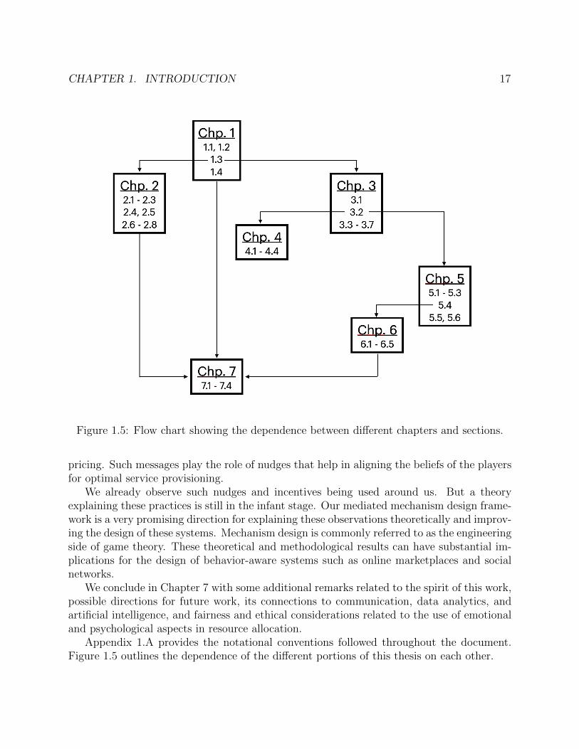
Appendix 1.A provides the notational conventions followed throughout the document.Figure 1.5 outlines the dependence of the different portions of this thesis on each other.

CHAPTER 1. INTRODUCTION 18
Appendix
1.A Notational Conventions
We introduce some notational conventions that will be used throughout the rest of thethesis. The scope of any additional notation introduced within a chapter will be limited tothat chapter.
Let N,Z,Q, and R denote the sets of all natural numbers, integers, rational numbers, andreal numbers, respectively. Let 1· denote the indicator function that is equal to one if thepredicate inside the brackets is true and is zero otherwise. Let supp(·) denote the supportof the probability distribution within the parentheses. If Z is a subset of a Euclidean space,then let co(Z) denote the convex hull of Z, and let co(Z) denote the closed convex hull ofZ. For any integer n ∈ N, let [n] := 1, 2, . . . , n.
If Z is a Polish space (complete separable metric space), let P(Z) denote the set ofall probability measures on (Z,F ), where F is the Borel sigma-algebra of Z. Let supp(p)denote the support of a distribution p ∈P(Z), i.e. the smallest closed subset of Z such thatp(Z) = 1. Let ∆f (Z) ⊂ P(Z) denote the set of all probability distributions that have afinite support. For any element p ∈ ∆f (Z), we will denote the probability of z ∈ Z assignedunder the distribution p by p(z) (or sometimes by p[z]). For z ∈ Z, let 1z ∈ ∆f (Z) denotethe probability distribution such that p(z) = 1. If Z is finite (and hence a Polish space withrespect to the discrete topology), let ∆(Z) denote the set of all probability distributions onthe set Z, viz.
∆(Z) = P(Z) = ∆f (Z) =
(p(z))z∈Z
∣∣∣∣p(z) ≥ 0 ∀z ∈ Z,∑z∈Z
p(z) = 1
,
with the usual topology. Let ∆m−1 denote the standard (m − 1)-simplex, i.e. ∆([m]). Fora function f : X → ∆(Y ), let f(y|x) = f(x)(y) denote the probability of y under theprobability distribution f(x).
LetL = (p1, z1); . . . ; (pt, zt).
denote a lottery with outcomes zj, 1 ≤ j ≤ t, with their corresponding probabilities givenby pj. We assume the lottery to be exhaustive (i.e.
∑tj=1 pj = 1). Note that we are allowed
to have pj = 0 for some values of j and we can have zk = zl even when k 6= l.If a lottery L consists of a unique outcome z that occurs with probability 1, then with
an abuse of notation we will denote the lottery L = (1, z) simply by L = z. Similarly, if aprobability distribution f(x) assigns probability 1 to y, then again with an abuse of notationwe will write f(x) = y. If, for each x, f(x) has a singleton support, then with an abuse ofnotation we will treat f as a function from X to Y .

CHAPTER 1. INTRODUCTION 19
Notes1Our focus here will be on decision under risk with outcome spaces mapped to real numbers but EUT
and CPT extend to more general settings with general outcome sets and subjective beliefs. See [132].2These assumptions are not needed for the results in this thesis to hold unless stated otherwise.3 The results in Chapter 2 appear in the paper [109].4 The results in Chapter 3 appear in the paper [108].5 The results in Chapter 4 appear in the pre-print [105].6 The results in Chapter 5 appear in the paper [106].7 The results in Chapter 6 appear in the pre-print [107].

20
Chapter 2
Optimal Resource Allocation overNetworks with CPT Players
2.1 Introduction
We consider the problem of congestion management in a network, and resource allocationamongst heterogeneous users, in particular human agents, with varying preferences. This isa well-recognized problem in network economics [94] and central to most of the examplesdiscussed in Section 1.2. Market-based solutions have proven to be very useful for thispurpose, with varied mechanisms, such as auctions and fixed rate pricing [46]. In thischapter, we consider a lottery-based mechanism, as opposed to the deterministic allocationsstudied in the literature. We mainly ask the following questions: (i) Do lotteries provide anadvantage over deterministic implementations? (ii) If yes, then does there exist a market-based mechanism to implement an optimum lottery?
In order to answer the first question we need to define our goal in allocating resources.There is an extensive literature on the advantages of lotteries: Eckhoff [43] and Stone [125]hold that lotteries are used because of fairness concerns; Boyce [21] argues that lotteriesare effective to reduce rent-seeking from speculators; Morgan [87] shows that lotteries arean effective way of financing public goods through voluntary funds, when the entity raisingfunds lacks tax power; Hylland and Zeckhauser [61] propose implementing lotteries to elicithonest preferences and allocate jobs efficiently. In all of these works, there is an underlyingassumption, which is also one of the key reasons for the use of lotteries, that the goods tobe allocated are indivisible.
However, we notice lotteries being implemented even when the goods to be allocated aredivisible, for example in lottos and parimutuel betting. In several experiments, it has beenobserved that lottery-based rewards are more appealing than deterministic rewards of thesame expected value, and thus provide an advantage in maximizing the desired influenceon people’s behavior [111]. We also observe several firms presenting lottery-based offers toincentivize customers into buying their products or using their services, and in return to

CHAPTER 2. NETWORK RESOURCE ALLOCATION 21
improve their revenues. Thus, although lottery-based mechanisms are being widely imple-mented, a theoretical understanding for the same seems to be lacking. This is one of themotivations for this chapter, which aims to justify the use of lottery-based mechanisms,based on models coming from behavioral economics for how humans evaluate options.
2.2 Lottery-Based Resource Allocation Model
We work with the framework proposed by Kelly [72] for throughput control in the Internetwith elastic traffic. However, this framework is general enough to have applications tonetwork resource allocation problems arising in several other domains. We have a networkwith a set [m] = 1, . . . ,m of resources or links and a set [n] = 1, . . . , n of users orplayers. Let cj > 0 denote the finite capacity of link j ∈ [m] and let c := (cj)j∈[m] ∈ Rm.(All vectors, unless otherwise specified, will be treated as column vectors.) Each user i hasa fixed route Ji, which is a non-empty subset of [m]. Let Rj := i ∈ [n]|j ∈ Ji the set of allplayers whose route uses link j. We say that an allocation profile x is feasible if it satisfiesthe capacity constraints of the network, i.e.∑
i∈Rj
xi ≤ ci,∀j ∈ [m]. (2.2.1)
Let F denote the set of all feasible allocation profiles. We assume that the network con-straints are such that F is bounded, and hence a polytope.
Instead of allocating a fixed throughput xi to player i ∈ [n], we consider allocating her alottery (or a prospect)
Li := (pi(1), yi(1)), . . . , (pi(ki), yi(ki)), (2.2.2)
where yi(li) ≥ 0, li ∈ [ki], denotes a throughput and pi(li), li ∈ [ki], is the probability withwhich throughput yi(li) is allocated.
We now describe the CPT model we use to measure the “utility” or “happiness” derivedby each player from her lottery. In order to focus on the effects of probabilistic sensitivity,and to avoid the complications resulting from reference point considerations, we assumethat the reference point of all the players is equal to 0, and we consider prospects withonly nonnegative outcomes. This is, in fact, identical to the rank dependent utility (RDU)model [114]. As a result, we assume that each player i is associated with a value functionvi : R+ → R+ that is continuous, differentiable, concave, and strictly increasing, and aprobability weighting function wi : [0, 1] → [0, 1] that is continuous, strictly increasing andsatisfies wi(0) = 0 and wi(1) = 1.8
For the prospect Li in (2.2.2), let πi : [ki]→ [ki] be a permutation such that
zi(1) ≥ zi(2) ≥ · · · ≥ zi(ki), (2.2.3)
andyi(li) = zi(πi(li)) for all li ∈ [ki]. (2.2.4)

CHAPTER 2. NETWORK RESOURCE ALLOCATION 22
The prospect Li can equivalently be written as
Li = (pi(1), zi(1)); . . . ; (pi(ki), zi(ki)),
where pi(li) := pi(π−1i (li)) for all li ∈ [ki]. The CPT value of prospect Li for player i
is evaluated using the value function vi(·) and the probability weighting function wi(·) asfollows:
Vi(Li) =
ki∑li=1
dli(pi, πi)vi(zi(li)), (2.2.5)
where dli(pi, πi) are the decision weights given by d1(pi, πi) := wi(pi(1)) and
dli(pi, πi) := wi(pi(1) + · · ·+ pi(li))− wi(pi(1) + · · ·+ pi(li − 1)),
for 1 < li ≤ ki. And equivalently, the CPT value of prospect Li, can be written as
Vi(Li) =
ki∑li=1
wi( li∑si=1
pi(si))
[vi(zi(li))− vi(zi(li + 1)))] ,
where zi(ki + 1) := 0. Thus the lowest allocation zi(ki) is weighted by wi(1) = 1, and everyincrement in the value of the allocations, vi(zi(li))− vi(zi(li + 1)),∀li ∈ [ki − 1], is weightedby the probability weighting function of the probability of receiving an allocation at leastequal to zi(li).
We take a utilitarian approach of maximizing the ex ante aggregate utility or the nethappiness of the players. (See [4] and the references therein for the relation with other goalssuch as maximizing revenue.) We then ask the question of finding the optimum allocationprofile of prospects, one for each user, comprised of throughputs and associated probabilitiesfor that user, that maximizes the aggregate utility of all the players, and is also feasible. Anallocation profile of prospects for each user is said to be feasible if it can be implemented, i.e.there exists a probability distribution over feasible throughput allocations whose marginalsfor each player agree with their allocated prospects.
We say that a lottery profile L1, . . . , Ln is feasible if there exists a joint distributionp ∈ ∆(
∏i[ki]) such that the following conditions are satisfied:
(i) The marginal distributions agree with Li for all players i, i.e.∑
l−ip(li, l−i) = pi(li) for
all li ∈ [ki], where l−i in the summation ranges over values in∏
i′ 6=i[ki′ ].
(ii) For each (li)i∈[n] ∈∏
i[ki] in the support of the distribution p (i.e. p((li)i∈[n]) > 0), theallocation profile (yi(li))i∈[n] is feasible.
Kelly suggested that the throughput allocation problem be posed as one of achievingmaximum aggregate utility for the users. In [73], he considers deterministic allocations andeach player has a utility function that determines her utility corresponding to an allocation.Its natural analog in our setup can be framed as the following optimization problem:
CHAPTER 2. NETWORK RESOURCE ALLOCATION 23
Maximizen∑i=1
Vi(Li)
subject to (i) and (ii)
The corresponding problem in [73] is a convex optimization problem and permits a de-composition into a central optimization problem and several user optimization problems,one for each user. Based on this decomposition, a market is proposed, in which each usersubmits an amount she is willing to pay per unit time to the network based on tentativerates that she received from the network; the network accepts these submitted amounts anddetermines the price of each network link. A user is then allocated a throughput in pro-portion to her submitted amount and inversely proportional to the sum of the prices of thelinks she wishes to use. Under certain assumptions, Kelly shows that there exist equilibriumprices and throughput allocations, and that these allocations achieve maximum aggregateutility. Thus the overall system problem of maximizing aggregate utility is decomposed intoa network problem and several user problems , one for each individual user. Further, in [73],the authors have proposed two classes of algorithms which can be used to implement arelaxation of the above optimization problem.
The optimization problem is our setting is more complicated than this. The two keyreasons for this are the non-convexity of the probability weighting functions and the per-mutation structure present in the computation of CPT value. In this chapter we will takea closer look at these aspects and see how we can get around these issues. We will ob-tain a user-network decomposition of the optimization problem that would give rise to amarket-based mechanism for optimal lottery allocations.
If all the players have EUT utility with concave utility functions, as is typically assumedto model risk-averseness, one can show that there exists a feasible deterministic allocationthat achieves the optimum and hence there is no need to consider lotteries. However, if theplayers’ utility is modeled by CPT, then one can improve over the best aggregate utilityobtained through deterministic allocations.
For example, Quiggin [115] considers the problem of distributing a fixed amount amongstseveral homogeneous players with RDU preferences. He concludes that, under certain condi-tions on players’ RDU preferences, the optimum allocation system is a lottery scheme with afew large prizes and a large number of small prizes, and is strictly preferred over distributingthe total amount deterministically amongst the players. In Section 2.7, we extend theseresults to network settings with heterogeneous players.
2.3 Discretization Trick
The distribution p and the throughputs (yi(li), i ∈ [n], li ∈ [ki]) of a feasible lottery profiletogether define a lottery scheme. In the following, we restrict our attention to specific typesof lottery schemes, wherein the network implements with equal probability one of the k

CHAPTER 2. NETWORK RESOURCE ALLOCATION 24
allocation profiles y(l) := (yi(l))i∈[n] ∈ Rn+, for l ∈ [k]. Let [k] = 1, . . . , k denote the setof outcomes, where allocation profile y(l) is implemented if outcome l occurs. Clearly, sucha scheme is feasible iff each of the allocation profiles y(l),∀l ∈ [k] belongs to F . Playeri thus faces the prospect Li = (1/k, yi(l))kl=1 and such a lottery scheme is completelycharacterized by the tuple y := (yi(l), i ∈ [n], l ∈ [k]). By taking k large enough, any lotteryscheme can be approximated by such a scheme.
Let yi := (yi(l))l∈[k] ∈ Rk+. Let zi := (zi(l))l∈[k] ∈ Rk+ be a vector and πi : [k] → [k] be apermutation such that
zi(1) ≥ zi(2) ≥ · · · ≥ zi(k),
andyi(l) = zi(πi(l)) for all l ∈ [k].
Note that yi is completely characterized by πi and zi. Then player i’s CPT value will be
Vi(Li) =k∑l=1
hi(l)vi(zi(l)),
where hi(l) := wi(l/k) − wi((l − 1)/k) for l ∈ [k]. Let hi := (hi(l))l∈[k] ∈ Rk+. Note thathi(l) > 0 for all i, l, since the weighting functions are assumed to be strictly increasing.
Looking at the lottery scheme y in terms of individual allocation profiles zi and permuta-tions πi for all players i ∈ [n], allows us to separate those features of y that affect individualpreferences and those that pertain to the network implementation. We will later see thatthe problem of optimizing aggregate utility can be decomposed into two layers: (i) a convexproblem that optimizes over resource allocations, and (ii) a non-convex problem that findsthe optimal permutation profile.
Let z := (zi(l), i ∈ [n], l ∈ [k]), π := (πi, i ∈ [n]), h := (hi(l), i ∈ [n], l ∈ [k]) andv := (vi(·), i ∈ [n]). Let Sk denote the set of all permutations of [k]. The problem ofoptimizing aggregate utility
∑i Vi(Li) subject to the lottery scheme being feasible, can be
formulated as follows:
SYS[z, π;h, v, A, c]
Maximizen∑i=1
k∑l=1
hi(l)vi(zi(l))
subject to∑i∈Rj
zi(πi(l)) ≤ cj, ∀j ∈ [m],∀l ∈ [k],
zi(l) ≥ zi(l + 1),∀i ∈ [n], ∀l ∈ [k],
πi ∈ Sk, ∀i ∈ [n].
We set zi(k + 1) = 0 for all i, and the zi(k + 1) are not treated as variables. This takes careof the condition zi(l) ≥ 0 for all i ∈ [n], l ∈ [k].
Note that such discretization serves in two ways:

CHAPTER 2. NETWORK RESOURCE ALLOCATION 25
• Instead of considering the non-convex probability weighting function wi for each playeri, we can restrict our attention to the vector hi := (hi(l), l ∈ [k]).
• It highlights the dependence on the permutation structure π.
In addition, the discretization also has a behavioral interpretation. Oftentimes, the play-ers are incapable of discerning the distinction between probabilities that are very close toeach other. They also show a poor sense of judgment when it comes to very small probabil-ities as one in a million. By restricting k say to be 100, we are making sure that the playersare faced with lotteries that have integer percentages which they can comprehend better.
Given a permutation profile, the problem of finding optimum feasible throughput al-locations is a convex programming problem, which we call the fixed-permutation systemproblem, and leads to a nice price mechanism. In the next section we prove the existenceof equilibrium prices that decompose the fixed-permutation system problem into a networkproblem and several user problems, one for each player, as in [72]. The prices can be inter-preted as the cost imposed on the players and can be implemented in several forms, such aswaiting times in waiting-line auctions or first-come-first-served allocations [12, 126], delay orpacket loss in the Internet TCP protocol [84, 76], efforts or resources invested by players ina contest [85, 31], or simply money or reward points.
Finding the optimum permutation profile, on the other hand, is a non-convex problem.In Section 2.6, we study the duality gap in the system problem and consider a relaxation ofthe system problem by allowing the permutations to be doubly stochastic matrices insteadof restricting them to be permutation matrices. We show that strong duality holds in therelaxed system problem and so it has value equal to the dual of the original system problem(Theorem 2.6.2). We also consider the problem where link constraints hold in expectation,called the average system problem, and show that strong duality holds in this case and so ithas value equal to the relaxed problem. In Section 2.7, we study the average system problemin further detail, and prove a result on the structure of optimal lotteries. We give an examplein Section 2.D to show that the duality gap in the original system problem can be nonzeroand Theorem 2.6.3 shows that the primal system problem is NP-hard.
2.4 Pricing and Market-Based Mechanism
The system problem SYS[z, π;h, v, A, c] optimizes over z and π. In this section we fix πi ∈ Skfor all i and optimize over z. Let SYS FIX[z; π, h, v, A, c] denote this fixed-permutation

CHAPTER 2. NETWORK RESOURCE ALLOCATION 26
system problem.
SYS FIX[z; π, h, v, A, c]
Maximizen∑i=1
k∑l=1
hi(l)vi(zi(l))
subject to∑i∈Rj
zi(πi(l)) ≤ cj,∀j ∈ [m],∀l ∈ [k],
zi(l) ≥ zi(l + 1),∀i ∈ [n],∀l ∈ [k].
(In contrast with SYS(z, π; . . . ), in SYS FIX(z; π, . . . ), the permutation π is thought of asbeing fixed.) Since vi(·) is assumed to be a concave function and hi(l) > 0 for all i, l, thisproblem has a concave objective function with linear constraints. For all j ∈ [m], l ∈ [k],let λj(l) ≥ 0 be the dual variables corresponding to the constraints
∑i∈Rj zi(πi(l)) ≤ cj
respectively, and for all i ∈ [n], l ∈ [k], let αi(l) ≥ 0 be the dual variables correspondingto the constraints zi(l) ≥ zi(l + 1) respectively. Let λ := (λj(l), j ∈ [m], l ∈ [k]) andα := (αi(t), i ∈ [n], l ∈ [k]). Then the Lagrangian for the fixed-permutation system problemSYS FIX[z; π, h, v, A, c] can be written as follows:
L (z;α, λ) :=n∑i=1
k∑l=1
hi(l)vi(zi(l))
+n∑i=1
k∑l=1
αi(l)[zi(l)− zi(l + 1)] +m∑j=1
k∑l=1
λj(l)[cj −∑i∈Rj
zi(πi(l))]
=n∑i=1
k∑l=1
[hi(l)vi(zi(l)) + (αi(l)− αi(l − 1))zi(l)−
(∑j∈Ji
λj(π−1i (l))
)zi(l)
]
+m∑j=1
k∑l=1
λj(l)cj,
where αi(0) = 0 for all i ∈ [n]. Differentiating the Lagrangian with respect to zi(l) we get,
∂L(z;α, λ)
∂zi(l)= hi(l)v
′i(zi(l)) + αi(l)− αi(l − 1)−
(∑j∈Ji
λj(π−1i (l))
).
Letρi(l) :=
∑j∈Ji
λj(π−1i (l)), (2.4.1)
for all i ∈ [n], l ∈ [k]. This can be interpreted as the price per unit throughput for playeri for her l-th largest allocation zi(l). The price of the lottery zi for player i is given by

CHAPTER 2. NETWORK RESOURCE ALLOCATION 27
∑kl=1 ρi(l)zi(l), or equivalently,
k∑l=1
µi(l) [zi(l)− zi(l + 1)] ,
where
µi(l) :=l∑
s=1
ρi(s), for all l ∈ [k]. (2.4.2)
For l ∈ [k − 1], αi(l) can be interpreted as a transfer of a nonnegative price for playeri from her l-th largest allocation to her (l + 1)-th largest allocation. Since the allocationzi(l + 1) cannot be greater than the allocation zi(l), there is a subsidy of αi(l) in the priceof zi(l) and an equal surcharge of αi(l) in the price of zi(l + 1). This subsidy and surchargeis nonzero (and hence positive) only if the constraint is binding, i.e. zi(l) = zi(l + 1). Onthe other hand, αi(k) is a subsidy in price given to player i for her lowest allocation, sinceshe cannot be charged anything higher than the marginal utility at her zero allocation.
Let hi := (hi(l))l∈[k] ∈ Rk+. Consider the following user problem for player i:
USER[mi;µi, hi, vi]
Maximizek∑l=1
hi(l)vi
(k∑s=l
mi(s)
µi(s)
)−
k∑l=1
mi(l)
subject to mi(l) ≥ 0,∀l ∈ [k],
(2.4.3)
where µi := (µi(l), l ∈ [k]) is a vector of rates such that
0 < µi(1) ≤ µi(2) ≤ · · · ≤ µi(k). (2.4.4)
We can interpret this as follows: User i is charged rate µi(k) for her lowest allocationδi(k) := zi(k). Let mi(k) denote the budget spent on the lowest allocation and hencemi(k) = µi(k)δi(k). For 1 ≤ l < k, she is charged rate µi(l) for the additional allocationδi(l) := zi(l) − zi(l + 1), beyond zi(l + 1) up to the next lowest allocation zi(l). Let mi(l)denote the budget spent on l-th additional allocation and hence mi(l) = µi(l)δi(l).
Let m := (mi(l), i ∈ [n], l ∈ [k]) and δ := (δi(l), i ∈ [n], l ∈ [k]). Consider the followingnetwork problem:
NET[δ;m,π,A, c]
Maximizen∑i=1
k∑l=1
mi(l) log(δi(l))
subject to δi(l) ≥ 0,∀i, ∀l,∑i∈Rj
k∑s=πi(l)
δi(s) ≤ cj,∀j,∀l.
CHAPTER 2. NETWORK RESOURCE ALLOCATION 28
This is the well known Eisenberg-Gale convex program [44] and it can be solved efficiently.Kelly et al. [73] proposed continuous time algorithms for finding equilibrium prices andallocations. For results on polynomial time algorithms for these problems see [64, 28]. Wehave the following decomposition result:
Theorem 2.4.1. For any fixed π, there exist equilibrium parameters µ∗,m∗, δ∗ and z∗ suchthat
(i) for each player i, m∗i solves the user problem USER[mi;µ∗i , hi, vi],
(ii) δ∗ solves the network problem NET[δ;m∗, π, A, c],
(iii) m∗i (l) = δ∗i (l)µ∗i (l) for all i, l,
(iv) δ∗i (l) = z∗i (l)− z∗i (l + 1) for all i, l, and
(v) z∗ solves the fixed-permutation system problem SYS FIX[z; π, h, v, A, c].
The proof of this can be found in Appendix 2.A.Thus the fixed-permutation system problem can be decomposed into user problems – one
for each player – and a network problem, for any fixed permutation profile π. Similar to theframework in [73], we have an iterative process as follows: The network presents each useri with a rate vector µi. Each user solves the user problem USER[mi;µi, hi, vi], and submitstheir budget vector mi, The network collects these budget vectors (mi)i∈[n] and solves thenetwork problem NET[δ;m∗, π, A, c] to get the corresponding allocation z (which can becomputed from the incremental allocations δ) and the dual variables λ. The network thencomputes the rate vectors corresponding to each user from these dual variables as given by(2.4.1) and (2.4.2) and presents it to the users as updated rates. Theorem 2.4.1 shows thatthe fixed-permutation system problem of maximizing the aggregate utility is solved at theequilibrium of the above iterative process. If the value functions vi(·) are strictly concave,then one can show that the optimal lottery allocation z∗ for the fixed-permutation systemproblem is unique. However, the dual variables λ, and hence the rates µi,∀i, need not beunique. Nonetheless, if one uses the continuous-time algorithm proposed in [73] to solve thenetwork problem, then a similar analysis as in [73], based on Lyapunov stability, shows thatthe above iterative process converges to the equilibrium lottery allocation z∗.
One of the permutation profiles, say π∗, solves the system problem. In Section 2.6, weexplore this in more detail. However, it is interesting to note that, for any fixed permutationprofile π, any deterministic solution is a special case of the lottery scheme y with permutationprofile π. Thus, it is guaranteed that the solution of the fixed-permutation system problem forany permutation profile π is at least as good as any deterministic allocation. Here is a simpleexample, where a lottery-based allocation leads to strict improvement over deterministicallocations.

CHAPTER 2. NETWORK RESOURCE ALLOCATION 29
0 0.2 0.4 0.6 0.8 10
0.2
0.4
0.6
0.8
1
pi
wi(p i
)
Figure 2.1: Probability weighting function for the example in Section 2.5. The plot showsthe probability weighting function given by equation (1.3.6) (also shown in Section 2.5) withγ = 0.61. The dotted line shows the identity function for reference.
2.5 A Quick Illustrative Example
Consider a network with n players and a single link with capacity c. Let n = 10 andc = 10. For all players i, we employ the value functions and weighting functions suggestedby Kahneman and Tversky [127], given by
vi(xi) = xβii , βi ∈ [0, 1],
and
wi(pi) =pγii
(pγi + (1− p)γi)1/γi, γi ∈ (0, 1],
respectively. We take βi = 0.88 and γi = 0.61 for all i ∈ [n]. These parameters were reportedas the best fits to the empirical data in [127]. The probability weighting function is displayedin Figure 2.1.
By symmetry and concavity of the value function vi(·), the optimal deterministic alloca-tion is given by allocating c/n to each player i. The aggregate utility for this allocation isn ∗ v1(c/n) = 10.
Now consider the following lottery allocation: Let k = n = 10. Let πi(l)−1 = l+i(mod k)for all i ∈ [n] and l ∈ [k]. Let x ∈ [c/n, c] and zi(1) = x for all i ∈ [n] and zi(l) = (c−x)/(n−1)for all i ∈ [n] and l = 2, . . . , k. Note that this is a feasible lottery allocation. Such a lotteryscheme can be interpreted as follows: Select a “winning” player uniformly at random fromall the players. Allocate her a reward x and equally distribute the remaining reward c − x

CHAPTER 2. NETWORK RESOURCE ALLOCATION 30
amongst the rest of the players. The ex ante aggregate utility is given by
n ∗ [w1(1/n)v1(x) + (1− w1(1/n))v1((c− x)/(n− 1))] .
This function achieves its maximum equal to 14.1690 at x = 9.7871. Thus, the above pro-posed lottery improves the aggregate utility over any deterministic allocation. The optimumlottery allocation is at least as good as 14.1690.
2.6 Optimum Permutation Profile and Duality Gap
The system problem SYS[z, π;h, v, A, c] can equivalently be formulated as
maxπi∈Sk∀i,
z:zi(l)≥zi(l+1)∀i,l
minλ≥0
n∑i=1
k∑l=1
hi(l)vi(zi(l))
+m∑j=1
k∑l=1
λj(l)
cj −∑i∈Rj
zi(πi(l))
.(I)
Let Wps denote the value of this problem. It is equal to the optimum value of the systemproblem SYS[z, π;h, v, A, c]. By interchanging the max and min, we obtain the followingdual problem:
minλ≥0
maxπi∈Sk∀i,
z:zi(l)≥zi(l+1)∀i,l
n∑i=1
k∑l=1
hi(l)vi(zi(l))
+m∑j=1
k∑l=1
λj(l)
cj −∑i∈Rj
zi(πi(l))
.(II)
Let Wds denote the value of this dual problem. By weak duality, we know that Wps ≤ Wds.For a fixed λ ≥ 0 and a fixed z that satisfies zi(l) ≥ zi(l+ 1),∀i, l, the optimum permutationprofile π in the dual problem (II) should minimize
m∑j=1
k∑l=1
λj(l)∑i∈Rj
zi(πi(l)),
which equals ∑i
∑l
ρi(l)zi(πi(l)),
Here ρi(l) :=∑
j∈Ji λj(l), is the price per unit allocation for player i under outcome l. Sincethe numbers zi(l) are ordered in descending order, any optimal permutation πi must satisfy
ρi(π−1i (1)) ≤ ρi(π
−1i (2)) ≤ · · · ≤ ρi(π
−1i (k)). (2.6.1)
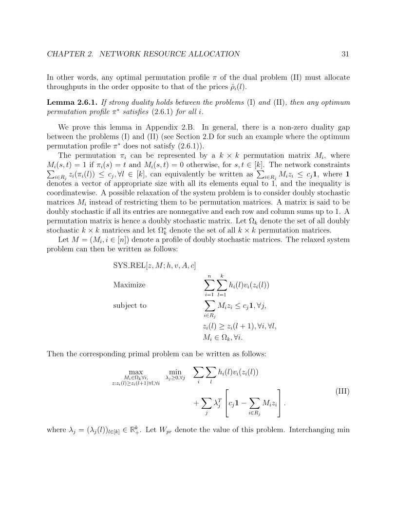
CHAPTER 2. NETWORK RESOURCE ALLOCATION 31
In other words, any optimal permutation profile π of the dual problem (II) must allocatethroughputs in the order opposite to that of the prices ρi(l).
Lemma 2.6.1. If strong duality holds between the problems (I) and (II), then any optimumpermutation profile π∗ satisfies (2.6.1) for all i.
We prove this lemma in Appendix 2.B. In general, there is a non-zero duality gapbetween the problems (I) and (II) (see Section 2.D for such an example where the optimumpermutation profile π∗ does not satisfy (2.6.1)).
The permutation πi can be represented by a k × k permutation matrix Mi, whereMi(s, t) = 1 if πi(s) = t and Mi(s, t) = 0 otherwise, for s, t ∈ [k]. The network constraints∑
i∈Rj zi(πi(l)) ≤ cj,∀l ∈ [k], can equivalently be written as∑
i∈Rj Mizi ≤ cj1, where 1denotes a vector of appropriate size with all its elements equal to 1, and the inequality iscoordinatewise. A possible relaxation of the system problem is to consider doubly stochasticmatrices Mi instead of restricting them to be permutation matrices. A matrix is said to bedoubly stochastic if all its entries are nonnegative and each row and column sums up to 1. Apermutation matrix is hence a doubly stochastic matrix. Let Ωk denote the set of all doublystochastic k × k matrices and let Ω∗k denote the set of all k × k permutation matrices.
Let M = (Mi, i ∈ [n]) denote a profile of doubly stochastic matrices. The relaxed systemproblem can then be written as follows:
SYS REL[z,M ;h, v, A, c]
Maximizen∑i=1
k∑l=1
hi(l)vi(zi(l))
subject to∑i∈Rj
Mizi ≤ cj1,∀j,
zi(l) ≥ zi(l + 1),∀i,∀l,Mi ∈ Ωk,∀i.
Then the corresponding primal problem can be written as follows:
maxMi∈Ωk∀i,
z:zi(l)≥zi(l+1)∀l,∀i
minλj≥0,∀j
∑i
∑l
hi(l)vi(zi(l))
+∑j
λTj
cj1−∑i∈Rj
Mizi
. (III)
where λj = (λj(l))l∈[k] ∈ Rk+. Let Wpr denote the value of this problem. Interchanging min

CHAPTER 2. NETWORK RESOURCE ALLOCATION 32
and max we get the corresponding dual:
minλj≥0,∀j
maxMi∈Ωk∀i,
z:zi(l)≥zi(l+1)∀l,∀i
∑i
∑l
hi(l)vi(zi(l))
+∑j
λTj
cj1−∑i∈Rj
Mizi
. (IV)
Let Wdr denote the value of this problem. If the link constraints in the relaxed systemproblem hold then
1
k
∑i∈Rj
k∑l=1
zi(l) =1
k
∑i∈Rj
1TMizi ≤1
k1T cj1 = cj. (2.6.2)
This inequality essentially says that the link constraints should hold in expectation. Thuswe have the following average system problem:
SYS AVG[z;h, v, A, c]
Maximizen∑i=1
k∑l=1
hi(l)vi(zi(l))
subject to∑i∈Rj
1
k
k∑l=1
zi(l) ≤ cj,∀j,
zi(l) ≥ zi(l + 1),∀i, ∀l,
with its corresponding primal problem:
maxz:zi(l)≥zi(l+1)∀l,∀i
minλj≥0,∀j
∑i
∑l
hi(l)vi(zi(l))
+∑j
λj
cj −∑i∈Rj
1
k
k∑l=1
zi(l)
, (V)
and the dual problem:
minλj≥0,∀j
maxz:zi(l)≥zi(l+1)∀l,∀i
∑i
∑l
hi(l)vi(zi(l))
+∑j
λj
cj −∑i∈Rj
1
k
k∑l=1
zi(l)
, (VI)
where λj ∈ R are the dual variables corresponding to the link constraints. Let Wpa and Wda
denote the values of these primal and dual problems respectively.Then we have the following relation:

CHAPTER 2. NETWORK RESOURCE ALLOCATION 33
Theorem 2.6.2. For any system problem defined by h, v, A and c, we have
Wps ≤ Wpr = Wpa = Wda = Wdr = Wds.
Proof given in Appendix 2.C.Thus the duality gap is a manifestation of the “hard” link constraints. In the proof of the
above theorem we saw that the relaxed problem is “equivalent” to the average problem andstrong duality holds for this relaxation. We will later study the average problem in furtherdetail (Section 2.7).
We observed earlier in Lemma 2.6.1 that if strong duality holds in the system problem,then the optimum permutation profile π∗ satisfies (2.6.1). Consider a simple example of twoplayers sharing a single link. Suppose that, at the optimum, λ(l) are the prices for l ∈ [k]corresponding to this link under the different outcomes, and suppose not all of these areequal. Then the optimum permutation profile of the dual problem will align both players’allocations in the same order, i.e. the high allocations of player 1 will be aligned with thehigh allocations of player 2. However, we can directly see from the system problem thatan optimum π∗ should align the two players’ allocations in opposite order. The example inAppendix 2.D builds on this observation and shows that strong duality need not hold forthe system problem.
Finally, we prove the following result in Appendix 2.E.
Theorem 2.6.3. The primal problem (I) is NP-hard.
2.7 Average System Problem and Optimal Lottery
Structure
Suppose it is enough to ensure that the link constraints are satisfied in expectation, as in theaverage system problem. As an example, suppose we are allocating resources to the playersrepeatedly and the links have buffers that allow us to allocate excess resources over theselinks provided the capacity constraints are satisfied on average. If the preferences of theplayers are not changing with time in this repeated setting, then we get the average systemproblem. More generally, we should allow the players’ preferences (and perhaps also thecapacity constraints) to change with time. We do not consider such a general setting here,however, as the average system problem solves a special case of this problem it would behelpful towards solving the general problem.
Consider the function V avgi (zi) on R+ given by the value of the following optimization

CHAPTER 2. NETWORK RESOURCE ALLOCATION 34
problem:
Maximizek∑l=1
hi(l)vi(zi(l))
subject to1
k
k∑l=1
zi(l) = zi,
zi(l) ≥ zi(l + 1), ∀l ∈ [k].
(VII)
Let Zi(zi) denote the set of feasible (zi(l))l∈[k] in the above problem for any fixed zi ≥ 0.We observe that Zi(zi) is a closed and bounded polytope, and hence V avg
i (zi) is well defined.
Lemma 2.7.1. For any continuous, differentiable, concave and strictly increasing value func-tion vi(·), the function V avg
i (·) is continuous, differentiable, concave and strictly increasingin zi.
We prove this lemma in Appendix 2.F. The average system problem SYS AVG[z;h, v, A, c]can be written as
Maximizen∑i=1
V avgi (zi)
subject to∑i∈Rj
zi ≤ cj,∀j,
zi ≥ 0,∀i.
Kelly [72] showed that this problem can be decomposed into user problems, one for eachuser i,
Maximize V avgi (zi)− ρizi
subject to zi ≥ 0,
and a network problem,
Maximizen∑i=1
ρizi
subject to∑i∈Rj
zi ≤ cj,∀j,
zi ≥ 0,∀i,
in the sense that there exist ρi ≥ 0, ∀i ∈ [n], such that the optimum solutions zi of theuser problems, for each i, solve the network problem and the average system problem. Notethat this decomposition is different from the one presented in Section 4.3. Here the networkproblem aims at maximizing its total revenue
∑ni=1 ρizi, instead of maximizing a weighted
aggregate utility where the utility is replaced with a proxy logarithmic function. The abovedecomposition is not as useful as the decomposition in Section 4.3 in order to develop iterative

CHAPTER 2. NETWORK RESOURCE ALLOCATION 35
schemes that converge to equilibrium. However, the above decomposition motivates thefollowing user problem:
USER AVG[zi; ρi, hi, vi]
Maximizek∑l=1
hi(l)vi(zi(l))−ρik
k∑l=1
zi(l)
subject to zi(l) ≥ zi(l + 1),∀l ∈ [k],
where, as before, zi(k + 1) = 0.We observed in Proposition 2.6.2 that strong duality holds in the average system problem.
Let z∗ be the optimum lottery scheme that solves this problem. Then, first of all, z∗ satisfiesz∗i (l) ≥ z∗i (l + 1) ∀i, l and is feasible in expectation, i.e., z∗ := (z∗i )i∈[n] ∈ F , where z∗i :=(1/k)
∑l z∗i (l). Further, z∗ optimizes the objective function of the average system problem.
Besides, there exist λ∗j ≥ 0 for all j such that the primal average problem (V) and the dualaverage problem (VI) each attain their optimum at z∗, (λ∗j , j ∈ [m]).
For player i, consider the price ρ∗i :=∑
j∈Ji λ∗j , which is obtained by summing the prices
λ∗j corresponding to the links on player i’s route. From the dual average problem (VI), fixingλj = λ∗j ∀j, we get that the optimum lottery allocation z∗i for player i should optimize theproblem USER AVG[zi; ρ
∗i , hi, vi].
We now impose some additional conditions on the probability weighting function thatare typically assumed based on empirical evidence and certain psychological arguments [67].We assume that the probability weighting function wi(pi) is concave for small values of theprobability pi and convex for the rest. Formally, there exists a probability pi ∈ [0, 1] such thatwi(pi) is concave over the interval pi ∈ [0, pi] and convex over the interval [pi, 1]. Typicallythe point of inflection, pi, is around 1/3.
Let w∗i : [0, 1] → [0, 1] be the minimum concave function that dominates wi(·), i.e.,w∗i (pi) ≥ wi(pi) for all pi ∈ [0, 1]. Let p∗i ∈ [0, 1] be the smallest probability such that w∗i (pi)is linear over the interval [p∗i , 1].
Lemma 2.7.2. Given the assumptions on wi(·), we have p∗i ≤ pi and w∗i (pi) = wi(pi) forpi ∈ [0, p∗i ]. If p∗i < 1, then for any p1
i ∈ [p∗i , 1), we have
wi(pi) ≤ wi(p1i ) + (pi − p1
i )1− wi(p1
i )
1− p1i
. (2.7.1)
for all pi ∈ [p1i , 1].
A proof of this lemma is included in Appendix 2.G. We now show that, under certainconditions, the optimal lottery allocation z∗i satisfies
z∗i (l∗) = z∗i (l
∗ + 1) = · · · = z∗i (k), (2.7.2)
where l∗ := minl ∈ [k] : (l − 1)/k ≥ p∗i , provided p∗i ≤ (k − 1)/k. As a result, fora typical optimum lottery allocation, the lowest allocation occurs with a large probabilityapproximately equal to 1−p∗i , and with a few higher allocations that we recognize as bonuses.

CHAPTER 2. NETWORK RESOURCE ALLOCATION 36
Proposition 2.7.3. For any average user problem USER AVG[zi; ρ∗i , hi, vi] with a strictly
increasing, continuous, differentiable and strictly concave value function vi(·), and a strictlyincreasing continuous probability weighting function wi(·) (satisfying wi(0) = 0 and wi(1) =1) such that p∗i ≤ (k − 1)/k, the optimum lottery allocation z∗i satisfies Equation (2.7.2).
Proof of this proposition is provided in Appendix 2.H.
2.8 Summary
We saw that if we take the probabilistic sensitivity of players into account, then lotteryallocation improves the ex ante aggregate utility of the players. We considered the RDUmodel, a special case of CPT utility, to model probabilistic sensitivity. This model, however,is restricted to reward allocations, and it would be interesting to extend it to a general CPTmodel with reference point and loss aversion. This will allow us to study loss allocations asin punishment or burden allocations, for example criminal justice, military drafting, etc.
For any fixed permutation profile, we showed the existence of equilibrium prices in amarket-based mechanism to implement an optimal lottery. We also saw that finding theoptimal permutation profile is an NP-hard problem. We note that the system problem hasparallels in cross-layer optimization in wireless [79] and multi-route networks [133]. Severalheuristic methods have helped achieve approximately optimal solutions in cross-layer opti-mization. Similar methods need to be developed for our system problem. We leave this forfuture work.
The hardness in the system problem comes from hard link constraints. Hence, by relaxingthese conditions to hold only in expectation, we derived some qualitative features of theoptimal lottery structure under the typical assumptions on the probability weighting functionof each agent in the RDU model. As observed, the players typically ensure their minimumallocation with high probability, and gamble for higher rewards with low probability.
We assumed that the players are price-takers, i.e. they respond optimally to the pricesshown to them in a myopic sense. Such an assumption is reasonable in situations wheneach player is a small participant in the system and does not have the ability to single-handedly influence the prices. However, more generally, one can imagine the players tobehave strategically and could try to manipulate the prices. For example, if a handful ofpeople are competing for a limited resource then they are prone to showing strategic behavioras opposed to the price-taking behavior assumed here. Analyzing such situations requiresstudying the strategic behavior of the players. In the following chapters, we undertake asystematic study of this by considering games with players having CPT preferences.
Appendix

CHAPTER 2. NETWORK RESOURCE ALLOCATION 37
2.A Proof of Theorem 2.4.1
Since SYS FIX[z; π, h, v, A, c] is a convex optimization problem, we know that there existz∗ = (z∗i (l), i ∈ [n], l ∈ [k]), α∗ = (α∗i (l), i ∈ [n], l ∈ [k]) and λ∗ = (λ∗j(l), j ∈ [m], l ∈ [k]) suchthat
hi(l)v′i(z∗i (l)) = ρ∗i (l)− α∗i (l) + α∗i (l − 1),∀i,∀l, (2.A.1)
z∗i (l) ≥ z∗i (l + 1), α∗i (l) ≥ 0, α∗i (l)(z∗i (l)− z∗i (l + 1)) = 0,∀i,∀l, (2.A.2)∑
i∈Rj
z∗i (πi(l)) ≤ cj, λ∗j(l) ≥ 0, λ∗j(l)[cj −∑i∈Rj
z∗i (πi(l))] = 0,∀j,∀l, (2.A.3)
whereρ∗i (l) :=
∑j∈Ji
λ∗j(π−1i (l)),
and such that z∗ solves the fixed-permutation system problem SYS FIX[z; π, h, v, A, c]. Hencestatement (v) holds for this choice of z∗. Let µ∗i (l) :=
∑ls=1 ρ
∗i (s), δ
∗i (l) := z∗i (l) − z∗i (l + 1)
and m∗i (l) := δ∗i (l)µ∗i (l) for all i, l. From (2.A.1), we have ρ∗i (1) > 0, because vi(·) is strictly
increasing, hi(1) > 0 and α∗i (0) = 0. Thus, the rate vector µ∗i satisfies (2.4.4) for all i. Alsonote that, by construction, the vectors µ∗, δ∗, z∗ and m∗ satisfy statements (iii) and (iv) ofthe theorem.
We now show that statement (i) holds. Fix a player i. Observe that the user problemUSER[mi;µ
∗i , hi, vi] has a concave objective function since hi(l) > 0, µ∗i (l) > 0 and vi(·) is
concave. Differentiating the objective function of the user problem USER[mi;µ∗i , hi, vi] with
respect to mi(l) at mi = m∗i , we get
l∑s=1
hi(s)v′i(z∗i (s))
µ∗i (l)− 1.
From (2.A.1), we have
l∑s=1
hi(s)v′i(z∗i (l)) =
l∑s=1
ρ∗i (s)− α∗i (l)
= µ∗i (l)− α∗i (l).
Thus,l∑
s=1
hi(s)v′i(z∗i (s))
µ∗i (l)− 1 = −α
∗i (l)
µ∗i (l)≤ 0,
where equality holds iff α∗i (l) = 0. If m∗i (l) > 0, then δ∗i (l) > 0 and hence, by (2.A.2),α∗i (l) = 0. Since this holds for all l ∈ [k], these are precisely the conditions necessary andsufficient for the optimality of m∗i in the problem of user i, it being a convex problem.

CHAPTER 2. NETWORK RESOURCE ALLOCATION 38
We now show that statement (ii) holds. The Lagrangian corresponding to the networkproblem NET[δ;m∗, π, A, c] can be written as follows:
L(δ;µ) =∑i
k∑l=1
m∗i (l) log(δi(l)) +∑j
∑l
µj(l)
cj −∑i∈Rj
k∑s=πi(l)
δi(s)
,where µj(l) is the dual variable corresponding to the link constraint and µ := (µj(l), j ∈[n], l ∈ [k]). Let µj(l) = λ∗j(l). If m∗i (l) > 0, then δ∗i (l) > 0, and differentiating theLagrangian with respect to δi(l) at δ∗i (l), we get
∂L(δ;λ∗)
∂δi(l)
∣∣∣∣∣δi(l)=δ∗i (l)
=m∗i (l)
δ∗i (l)−∑j∈Ji
l∑s=1
λ∗j(π−1i (s))
= r∗i (l)−l∑
s=1
ρ∗i (s) = 0.
If m∗i (l) = 0, then ∂L(δ;λ∗)∂δi(l)
∣∣δi(l)=δ∗i (l)
≤ 0 since λ∗j(l) ≥ 0 for all j, l. Further, from (2.A.3), we
have λ∗j(l)[cj −
∑i∈Rj
∑ks=πi(l)
δ∗i (s)]
= 0 for all j, l. Thus, δ∗ solves the network problem
NET[δ;m∗, π, A, c].
2.B Proof of Lemma 2.6.1
Suppose problem (I) and its dual (II) have the same value. The value of (I) is same as thatof the system problem SYS[z, π;h, v, A, c]. Let us denote the objective function by
Θ(π, z, λ) :=n∑i=1
k∑l=1
hi(l)vi(zi(l))
+m∑j=1
k∑l=1
λj(l)
cj −∑i∈Rj
zi(πi(l))
.Since F is a polytope, for any fixed permutation profile π, the set of feasible z is closedand bounded. The function Θ(π, z, λ) is continuous in z and hence the fixed-permutationsystem problem SYS FIX[z; π, h, v, A, c] has a bounded value. We also note that this value isnon-negative. Since there are finitely many permutation profiles π ∈
∏i Sk, maximizing over
these, we get that the system problem has a bounded non-negative value, say W , achievedsay at z∗ and π∗. Thus
n∑i=1
k∑l=1
hi(l)vi(z∗i (l)) = W, (2.B.1)

CHAPTER 2. NETWORK RESOURCE ALLOCATION 39
and the lottery z∗ is feasible with respect to the permutation profile π∗, i.e. z∗i (l) ≥ z∗i (l+ 1)for all i ∈ [n], l ∈ [k] and ∑
i∈Rj
z∗i (π∗i (l)) ≤ cj for all j ∈ [m], l ∈ [k]. (2.B.2)
If this were not true, then the minimum of the objective function Θ(π∗, z∗, λ) with respectto λ would be −∞ and not W ≥ 0.
The value of the dual problem (II) is equal to W . Consider the function Θd : Rm×k+ → R,given by maximizing over the objective function in problem (II), with respect to π and z fora fixed λ ≥ 0,
Θd(λ) := maxπi∈Sk∀i,
z:zi(l)≥zi(l+1)∀i,l
Θ(π, z, λ).
We note that the function Θd(λ) is lower semi-continuous, since the function Θ(π, z, λ) iscontinuous in λ. Since (vi(·),∀i) are concave strictly increasing functions, there exists asufficiently large finite λ such that 0 ≤ M := Θd(λ) < ∞. It follows that the minimum ofΘd(λ) is achieved over the domain defined by λj(l) ∈ [0,M/(minj cj)] for all j, l. Since thisis a bounded region and the function Θd(λ) is lower semi-continuous, there exists a λ∗ suchthat Θd(λ
∗) = minλ≥0 Θd(λ) = W .Since Θd(λ
∗) = W , we have Θ(π∗, z∗, λ∗) ≤ W . However, from (2.B.1), (2.B.2) and thefact that λ∗j(l) ≥ 0 for all j, l we get Θ(π∗, z∗, λ∗) ≥ W . Hence Θ(π∗, z∗, λ∗) = W . Thus themaximum in the definition of Θd(λ
∗) is achieved at z∗, π∗. This implies π∗i satisfies (2.6.1)for all i.
2.C Proof of Proposition 2.6.2
As observed earlier, if we replace the condition Mi ∈ Ωk in the primal relaxed problem (III)with the condition Mi ∈ Ω∗k, we get the primal system problem (I). Since Ω∗k ⊂ Ωk, we haveWps ≤ Wpr.
The constraint∑
i∈Rj1k
∑kl=1 zi(l) ≤ cj can equivalently be written as∑
i∈Rj
Mizi ≤ cj1,
for all j, where Mi is the matrix with all its entries equal to 1/k. Thus, if we replace Mi ∈ Ωk
in the primal relaxed problem (III) with Mi, we get the primal average problem (V). Thisimplies that Wpa ≤ Wpr. However, as observed earlier in Equation (2.6.2), if for some fixedallocations z the link constraints are satisfied with respect to any doubly stochastic matrixMi, then they are also satisfied with respect to Mi. Thus the maximum of the average systemproblem SYS AVG[z;h, v, A, c] is at least as much as the maximum of the relaxed system

CHAPTER 2. NETWORK RESOURCE ALLOCATION 40
problem SYS REL[h, v, A, c]. Since the maximum of the relaxed system problem is equal tothe value of its corresponding primal problem, we get Wpa ≥ Wpr. Thus, we have establishedthat Wpr = Wpa.
The average system problem has a concave objective function with linear constraints.Thus, strong duality holds, and we get Wpa = Wda.
We now show that Wda = Wdr. From Wpr ≤ Wdr and Wpr = Wpa = Wda, we getWda ≤ Wdr. Suppose λj = λj1. Then the objective function of the relaxed dual problem (IV),
n∑i=1
k∑l=1
hi(l)vi(zi(l)) +m∑j=1
λTj
cj1−∑i∈Rj
Mizi
=
n∑i=1
k∑l=1
hi(l)vi(zi(l)) +m∑j=1
λj
cj −∑i∈Rj
1
k
k∑l=1
zi(l)
,equals the objective function of the dual average problem (V). This implies that Wdr ≤ Wda.This established that Wda = Wdr.
Since any doubly stochastic matrix Mi is a convex combination of permutation matricesby the Birkhoff-von Neumann theorem, in the dual problem (IV), for any fixed λj, zi, theoptimum can be achieved by a permutation matrix. This established that Wdr = Wds.
This completes the proof.
2.D Example to Show Duality Gap
Consider the following example with two players 1, 2 and a single link with capacity 2.9.Let k = 2. Let the corresponding CPT characteristics of the two players be as follows:
h1(1) =1
3, h1(2) =
2
3,
h2(1) =5
6, h2(2) =
1
6,
v1(x) = log(x+ 0.05) + 3, v2(x) =2 log(x+ 0.05) + 3(x+ 0.05)
5+ 3.
For this problem, it is easy to see that π1 = (1, 2) and π2 = (2, 1) is an optimal permuta-tion. Solving the fixed-permutation system problem with respect to this permutation we getoptimal value equal to 7.5621. The corresponding variable values are
z1(1) = y1(1) = 1.95, z1(2) = y1(2) = 0.95,
z2(1) = y2(2) = 1.95, z2(2) = y2(1) = 0.95,
and the dual variable values are
λ1(1) =1
6, λ1(2) =
2
3,

CHAPTER 2. NETWORK RESOURCE ALLOCATION 41
and αi(l) = 0, for i = 1, 2, l = 1, 2. One can check that these satisfy the KKT conditions.Let us now evaluate the value of the dual problem (II). By symmetry, we can assume
without loss of generality that λ1(1) ≤ λ1(2). As a result, optimal permutations for the dualproblem are given by π1 = π2 = (1, 2). For fixed λ1(1) and λ1(2), we solve the followingoptimization problem:
maxz1(1)≥z1(2)≥0z2(1)≥z2(2)≥0
1
3log(z1(1) + 0.05) +
2
3log(z1(2) + 0.05)
+5
6
[2 log(z2(1) + 0.05) + 3(z2(1) + 0.05)
5
]+
1
6
[2 log(z2(2) + 0.05) + 3(z2(2) + 0.05)
5
]− λ1(1)[z1(1) + z2(1)]− λ1(2)[z1(2) + z2(2)]
+ 2.9[λ1(1) + λ1(2)] + 6.
(VIII)
If λ1(1) ≤ 0.5, then the value of the problem (VIII) is equal to ∞ (let z2(1) → ∞).If λ1(1) > 0.5 (and hence λ1(2) > 0.5 because λ1(2) ≥ λ1(2)), then we observe that theeffective domain of maximization in the problem (VIII) is compact and problem (VIII) hasa finite value. Hence it is enough to consider λ1(1) > 0.5. At the optimum there existα1(1), α1(2), α2(1), α2(2) ≥ 0 such that
λ1(1) =1
3
1
z1(1) + 0.05+ α1(1),
λ1(2) =2
3
1
z1(2) + 0.05− α1(1) + α1(2),
λ1(1) =1
3
1
z2(1) + 0.05+
1
2+ α2(1),
λ1(2) =1
15
1
z2(2) + 0.05+
1
10− α2(1) + α2(2),
and
α1(1)[z1(1)− z1(2)] = 0, α1(2)z1(2) = 0,
α2(1)[z2(1)− z2(2)] = 0, α2(2)z2(2) = 0.
We now consider each of the sixteen (4 × 4) cases based on whether the inequalitieszi(l) ≥ zi(l + 1) for i = 1, 2 and l = 1, 2, hold strictly or not.
Case A1 (z1(1) = 0, z1(2) = 0). Then λ1(1) ≥ 1/0.15.Case B1 (z1(1) > 0, z1(2) = 0). Then λ1(1) < 1/0.15, λ1(2) ≥ 2/0.15, and
α1(1) = 0, z1(1) =1
3λ1(1)− 0.05.

CHAPTER 2. NETWORK RESOURCE ALLOCATION 42
B2 D2C1 10.2284 8.2757D1 10.1814 9.5006
Table 2.D.1: Table showing the numerical evaluations corresponding to the example inSection 2.D. The numbers in the cells denote the optimum value of the objective function(VIII) in the corresponding cases.
Case C1 (z1(1) = z1(2) > 0). Then λ1(2)/2 ≤ λ1(1) ≤ λ1(2), λ1(1) + λ1(2) < 1/0.05,and
α1(1) =2λ1(1)− λ1(2)
3, α1(2) = 0, z1(1) = z1(2) =
1
λ1(1) + λ1(2)− 0.05.
Case D1 (z1(1) > z1(2) > 0). Then λ1(1) < λ1(2)/2, 0 < λ1(1) < 1/0.15, 0 < λ1(2) <2/0.15, and
α1(1) = 0, α1(2) = 0, z1(1) =1
3λ1(1)− 0.05, z1(2) =
2
3λ1(2)− 0.05.
Case A2 (z2(1) = 0, z2(2) = 0). Then λ1(1) ≥ (1/0.15) + 0.5.Case B2 (z2(1) > 0, z2(2) = 0). Then 0.5 < λ1(1) < 2.15/0.3, λ1(2) ≥ (1/0.75) + 0.1,
and
α2(1) = 0, z2(1) =2
6λ1(1)− 3− 0.05.
Case C2 (z2(1) = z2(2) > 0). This is not possible since λ1(1) ≤ λ1(2).Case D2 (z2(1) > z2(2) > 0). Then 0.5 < λ1(1) < 2.15/0.3, 0.1 < λ1(2) < 2.15/1.5, and
α2(1) = 0, α2(2) = 0, z2(1) =2
6λ1(1)− 3− 0.05, z2(2) =
2
30λ1(2)− 3− 0.05.
If case A1 or case A2 holds, then λ1(1) ≥ 1/0.15. For any fixed λ1(1), λ1(2), by choosingzi(l), i = 1, 2, l = 1, 2 small enough (respecting the conditions imposed by the correspondingcases), we get that the value of problem (VIII) is greater than or equal to 2.9 ∗ (1/0.15) =19.3333 > 7.5621. Similarly, if case B1 holds, then λ1(2) ≥ 2/0.15, and we get that the valueof problem (VIII) is greater than or equal to 2.9 ∗ (2/0.15) = 38.6667 > 7.5621. For theremaining 4 cases, substituting the corresponding expressions for zi(l), i = 1, 2, l = 1, 2 inthe objective function (VIII) and evaluating the optimum over feasible pairs (λ1(1), λ1(2))for each pair of cases C1,D1 × B2,D2, the minimum is achieved for the case (C1,D2)and has value equal to 8.2757. Numerical evaluation for each of these cases gives rise to theminimum values as shown in Table 2.D.1. Thus the optimal dual value is 8.2757 and this isstrictly greater than the primal value.

CHAPTER 2. NETWORK RESOURCE ALLOCATION 43
2.E Proof of Theorem 2.6.3
We describe a polynomial time procedure that reduces an instance of the integer parti-tion problem to a special case of the primal problem. Given a set of positive integersc1, c2, . . . , cn, the integer partition problem is to find a subset S ⊂ [n], such that∑
i∈S
ci =∑i/∈S
ci.
If such a set S exists, then we say that an integer partition exists. Consider a network withn players and n+ 1 link constraints given by
yi ≤ ci,∀i ∈ [n], andn∑i=1
yi ≤∑n
i=1 ci2
.
It is easy to realize a network with these link constraints. Let k = 2. Let the CPT charac-teristics of all the players be as follows:
hi(1) = 1− ε, hi(2) = ε, vi(xi) = xi,∀i ∈ [n],
where ε = 1/10. Let Wps denote the optimal value of the system problem. We show thatWps ≥ T := (1 − ε)
∑i∈[n] ci if and only if an integer partition exists. Suppose an integer
partition exists and is given by the set S, consider the allocation πi = [1, 2] if i ∈ S andπi = [2, 1] otherwise, zi(1) = ci, zi(2) = 0 for all i ∈ [n]. The aggregate utility for thisallocation is equal to T and hence Wps ≥ T . Suppose Wps ≥ T . Then there an allocation,say z∗ and π∗ with aggregate utility at least T . Since k = 2, π∗ actually defines a partitionof [n], given by S = i ∈ [n] : πi(1) = 1. We have, the aggregate utility
W (1) +W (2) ≥ T,
where
W (1) :=∑i∈S
(1− ε)zi(1) +∑i/∈S
εzi(2),
W (2) :=∑i/∈S
(1− ε)zi(1) +∑i∈S
εzi(2).
Hence at least one of W (1) and W (2 is at least as big as T/2. Without loss of generality, letW (1) ≥ T/2. Thus we have,∑
i∈S
zi(1) +ε
1− ε∑i/∈S
zi(2) ≥∑
i∈[n] ci
2.
However, since z∗ is feasible, the link constraints give∑i∈S
zi(1) +∑i/∈S
zi(2) ≤∑
i∈[n] ci
2.
Since ε < 1/2, we should have∑
i/∈S zi(2) = 0 and∑
i∈S zi(1) = (∑
i∈[n] ci)/2, implying thatS forms an integer partition. This completes the proof.

CHAPTER 2. NETWORK RESOURCE ALLOCATION 44
2.F Proof of Lemma 2.7.1
Let zi ≥ 0 and τ > 0. Let z∗i ∈ Zi(zi) be such that V avgi (zi) =
∑kl=1 hi(l)vi(z
∗i (l)). We have,
(z∗i (l) + τ)l∈[k] ∈ Zi(zi + τ) and
V avgi (zi + τ) ≥
k∑l=1
hi(l)vi(z∗i (l) + τ) >
k∑l=1
hi(l)vi(z∗i (l)) = V avg
i (zi),
where the strict inequality follows from the fact that vi(·) is strictly increasing. This estab-lishes that the function V avg
i (zi) is strictly increasing.Let z1
i , z2i ≥ 0 and σ ∈ [0, 1]. Let z1
i ∈ Zi(z1i ) and z2
i ∈ Zi(z2i ) be such that V avg
i (z1i ) =∑k
l=1 hi(l)vi(z1i (l)) and V avg
i (z2i ) =
∑kl=1 hi(l)vi(z
2i (l)). Let zσi := σz1
i (l) + (1 − σ)z2i (l) and
zσi := σz1i (l) + (1− σ)z2
i (l). Then zσi ∈ Zi(zσi ) and by the concavity of vi(·), we have
V avgi (zσi ) ≥
k∑l=1
hi(l)vi(zσi (l)) ≥
k∑l=1
hi(l)[σvi(z
1i (l)) + (1− σ)vi(z
2i (l))
]= σV avg
i (z1i ) + (1− σ)V avg
i (z2i ).
This establishes that the function V avgi (zi) is concave. This implies that V avg
i (zi) is continuousand directionally differentiable at each zi > 0, and we have the following relation betweenits left and right directional derivatives (see, for example, [117]):
d
dziV avgi (zi−) ≥ d
dziV avgi (zi+), for all zi > 0. (2.F.1)
Further, if (zti)t≥1 is a sequence such that zti → 0, and zti ∈ Zi(zti) for all t ≥ 1, then zti(l)→ 0for all l ∈ [k]. By the continuity of the function vi(·), we have that the function V avg
i (zi) iscontinuous at zi = 0.
Let zi > 0, and let τ t := 1/t, for t ≥ 1. As before, let z∗i ∈ Zi(zi) be such that V avgi (zi) =∑k
l=1 hi(l)vi(z∗i (l)). Since zi > 0 and (1/k)
∑kl=1 z
∗i (l) = zi, we have z∗i (l) > z∗i (l + 1) for at
least one l ∈ [k]. Let l ∈ [k] be the smallest such l. For t ≥ 1, let zt+i be given by
zt+i (l) :=
z∗i (l) + k
lτ t, for 1 ≤ l ≤ l,
z∗i (l), for l < l ≤ k.
Note that zt+i ∈ Zi(zi + τ t). We have,
V avgi (zi + τ t)− V avg
i (zi)−kτ t
l
l∑l=1
hi(l)v′i(z∗i (l))
≥k∑l=1
hi(l)vi(zt+i (l))−
k∑l=1
hi(l)vi(z∗i (l))−
kτ t
l
l∑l=1
hi(l)v′i(z∗i (l))
=l∑l=1
hi(l)
[vi(z
∗i (l) + kτ t/l)− vi(z∗i (l))−
kτ t
lv′i(z
∗i (l))
].

CHAPTER 2. NETWORK RESOURCE ALLOCATION 45
Let γ∗ := k
l
∑ll=1 hi(l)v
′i(z∗i (l)). We have,
d
dziV avgi (zi+) ≥ lim inf
t→∞
V avgi (zi + τ t)− V avg
i (zi)
τ t≥ γ∗. (2.F.2)
Similarly, for t ≥ dk/z∗i (l)e (here, d·e denotes the ceiling function), let zt−i be given by
zt−i (l) :=
z∗i (l)− k
lτ t, for 1 ≤ l ≤ l,
z∗i (l), for l < l ≤ k.
We observe that zt−i ∈ Zi(zi − τ t), for all t ≥ dk/z∗i (l)e, and we have
V avgi (zi)− V avg
i (zi − τ t)−kτ t
l
l∑l=1
hi(l)v′i(z∗i (l))
≤k∑l=1
hi(l)vi(z∗i (l))−
k∑l=1
hi(l)vi(zt−i (l))− kτ t
l
l∑l=1
hi(l)v′i(z∗i (l))
=l∑l=1
hi(l)
[vi(z
∗i (l))− vi(z∗i (l)− kτ t/l)−
kτ t
lv′i(z
∗i (l))
].
This implies,d
dziV avgi (zi−) ≤ lim sup
t→∞
V avgi (zi)− V avg
i (zi − τ t)τ t
≤ γ∗. (2.F.3)
From (2.F.1), (2.F.2) and (2.F.3), we have
d
dziV avgi (zi−) =
d
dziV avgi (zi+) = γ∗. (2.F.4)
This establishes that the function V avgi (zi) is differentiable and completes the proof.
2.G Proof of Lemma 2.7.2
Consider the function wi : [0, 1]→ [0, 1], given by
wi(pi) :=
w∗i (pi) for 0 ≤ pi < pi,
w∗i (pi) + (pi − pi)1−w∗i (pi)
1−pi for pi ≤ pi ≤ 1.
Since w∗i is concave on [0, 1], one can verify that the function wi is also concave on [0, 1].Since w∗i dominates wi, we have w∗i (pi) ≥ wi(pi). Since the function wi(pi) is convex on theinterval [pi, 1], we have wi(pi) ≤ wi(pi), for pi ∈ [pi, 1]. However, since w∗i is the minimum

CHAPTER 2. NETWORK RESOURCE ALLOCATION 46
concave function that dominates wi, we get wi = w∗i . Thus, w∗i is linear over the interval[pi, 1], and hence p∗i ≤ pi.
Suppose pi = 1. Then wi(·) is a concave function on the unit interval [0, 1], and hencew∗i (pi) = wi(pi), for pi ∈ [0, 1] ⊃ [0, p∗i ]. Further, if p∗i < 1, then wi(pi) is linear over [p∗i , 1],and inequality (2.7.1) holds, in fact, with equality. This completes the proof of Lemma 2.7.2,if pi = 1.
For the rest of the proof we assume pi < 1. Define gi : [0, 1)→ R+ as
gi(pi) :=1− wi(pi)
1− pi.
We now provide an alternate characterization of the function w∗i and the point p∗i . Letpi ∈ [0, 1] be given by
pi := min arg minpi∈[0,pi]
g(pi) .
The existence of pi is guaranteed by the continuity of the function gi(pi) on the compactinterval [0, pi]. Let ai := gi(pi). Since wi(pi) is convex over the interval [pi, 1], the functiongi(pi) is non-decreasing over [pi, 1). Hence gi(pi) ≥ gi(pi), for pi ∈ [0, 1). Substituting theexpression for gi(·) and rearranging, we get
wi(pi) ≤ wi(pi) + ai(pi − pi),
for pi ∈ [0, 1]. Since the function wi(pi) is concave on the interval [0, pi] and the linearfunction wi(pi) + ai(pi − pi) dominates wi(pi) on [0, 1], we have that the following functionwi(pi) is concave on [0, 1]:
wi(pi) :=
wi(pi) for 0 ≤ pi < pi,
wi(pi) + ai(pi − pi) for pi ≤ pi ≤ 1.
It follows that w∗i (pi) = wi(pi) for pi ∈ [0, 1]. Thus, p∗i ≤ pi and w∗i (pi) = wi(pi) = wi(pi)for pi ∈ [0, p∗i ]. If pi = 0, then p∗i = pi. If pi > 1, then from the definition of pi, we havegi(pi) > gi(pi) for pi ∈ [0, pi), and this implies that pi = p∗i .
We now prove inequality (2.7.1). Since pi < 1 we have p∗i < 1. Rearranging we get thatinequality (2.7.1) is equivalent to showing that the function gi(pi) is non-decreasing over theinterval [p∗i , 1). As observed earlier, gi(pi) is non-decreasing over the interval [pi, 1). Henceit is enough to show that the function gi(pi) is non-decreasing on [p∗i , pi]. Suppose, on thecontrary, there exist p1
i , p2i ∈ [p∗i , pi] such that p1
i < p2i and gi(p
1i ) > gi(p
2i ). Since p∗i = pi, and
from the definition of pi, we have p1i > p∗i and gi(p
∗i ) ≤ gi(p
2i ). Since, gi(pi) is a continuous
function, there exist pi ∈ [p∗i , p1i ) such that gi(pi) = gi(p
2i ). Thus we have pi < p1
i < p2i such
that gi(p1i ) > gi(pi) = gi(p
2i ). However, this contradicts the concavity of wi(pi) on [p∗i , pi].
This completes the proof.

CHAPTER 2. NETWORK RESOURCE ALLOCATION 47
2.H Proof of Proposition 2.7.3
The Lagrangian for the average user problem USER AVG[zi; ρ∗i , hi, vi] is
L(zi;αi) =k∑l=1
hi(l)vi(zi(l))−ρ∗ik
k∑l=1
zi(l) +k∑l=1
αi(l)[zi(l)− zi(l + 1)],
where αi(l) ≥ 0 are the dual variables corresponding to the order constraints zi(l) ≥ zi(l+1),and αi(0) = 0. Differentiating with respect to zi(l), we get,
∂L(zi;αi)
∂zi(l)= hi(l)v
′i(zi(l))−
ρ∗ik
+ αi(l)− αi(l − 1).
Since the problem USER AVG[zi; ρ∗i , hi, vi] has a concave objective function and linear con-
straints, there exist α∗i (l) ≥ 0 such that
hi(l)v′i(z∗i (l)) =
ρ∗ik− α∗i (l) + α∗i (l − 1),∀l ∈ [k], (2.H.1)
and
α∗i (l)[z∗i (l)− z∗i (l + 1)] = 0, ∀l ∈ [k]. (2.H.2)
If z∗i consists of identical allocations then it trivially satisfies Equation (2.7.2). If not, thenthere exists l1 ∈ 2, . . . , k such that
z∗i (l1 − 1) > z∗i (l
1) = z∗i (l1 + 1) = · · · = z∗i (k),
i.e. z∗i (l1) is the lowest allocation and occurs with probability (k − l1 + 1)/k, and the next
lowest allocation is equal to z∗i (l1 − 1). Summing the equations corresponding to l1 ≤ l ≤ k
from (2.H.1), we get[k∑
s=l1
hi(s)
]v′i(z
∗i (l
1)) =
(k − l1 + 1
k
)ρ∗i − α∗i (k) + α∗i (l
1 − 1). (2.H.3)
The equation corresponding to l = l1 − 1 in (2.H.1) says,
hi(l1 − 1)v′i(z
∗i (l
1 − 1)) =ρ∗ik− α∗i (l1 − 1) + α∗i (l
1 − 2). (2.H.4)
Since z∗i (l1 − 1) > z∗i (l
1), from (2.H.2), we have α∗i (l1 − 1) = 0. Thus from (2.H.3) and
(2.H.4), we have
hi(l1 − 1)v′i(z
∗i (l
1 − 1)) ≥ ρ∗ik≥ 1
k − l1 + 1
[k∑
s=l1
hi(s)
]v′i(z
∗i (l
1)).

CHAPTER 2. NETWORK RESOURCE ALLOCATION 48
Further, since vi(·) is strictly concave and strictly increasing, z∗i (l1 − 1) > z∗i (l
1) implies0 < v′i(z
∗i (l
1 − 1) < v′i(z∗i (l
1)). Thus,
hi(l1 − 1) >
1
k − l1 + 1
[k∑
s=l1
hi(s)
]. (2.H.5)
If (l1 − 2)/k ≥ p∗i , then
hi(l1 − 1) = wi
(l1 − 1
k
)− wi
(l1 − 2
k
)≤ 1
k − l1 + 1
[wi(1)− wi
(l1 − 1
k
)]=
1
k − l1 + 1
[k∑
s=l1
hi(s)
]. (2.H.6)
where the inequality follows from (2.7.1) with p1i = (l1− 2)/k and pi = (l1− 1)/k. However,
(2.H.6) contradicts (2.H.5) and hence (l1 − 2)/k < p∗i . This proves the lemma.
Notes8 In this chapter, for brevity, we drop the notation of reference point r from vri , and the positive sign
from the probability weighting function w+i .

49
Chapter 3
Notions of Equilibrium: CPT NashEquilibrium and CPT CorrelatedEquilibrium
3.1 Introduction
Non-cooperative game theory studies the interaction between decision makers with possiblydifferent objectives. The decision-makers are generally modeled as expected utility maximiz-ers. We will consider games where players have cumulative prospect theoretic preferences.Two of the most well known notions of equilibrium, Nash equilibrium [99] and correlatedequilibrium [6], are based on EUT. (See [75] for an excellent account of the strengths andweaknesses of these notions.) Keskin [74] defines analogs for both these equilibrium notionsbased on cumulative prospect theory. He also establishes the existence of such equilibriaunder certain continuity conditions. In this chapter, we further study several interestingproperties of these notions of equilibria.
There has been considerable interest in the study of the comparative geometry of Nashand correlated equilibria. Under EUT, it is known that the set of all correlated equilibria isa convex polytope and contains the set of all Nash equilibria. In the paper [101], it has beenproved that:
the Nash equilibria all lie on the boundary of the correlated equilibrium poly-tope.
(P)
Further, it has been found that in 2-player (bimatrix) games, all extremal Nash equilibriaare also extremal correlated equilibria [38, 26, 45], although this result does not hold formore than 2 players [101]. We give a complete characterization of the sets of correlated andNash equilibria for 2x2 games under CPT, with EUT being a special case.9
CPT is known to share common features with EUT. Indeed, recall that CPT is a gener-alization of EUT. The purpose of this chapter is to study how the geometry of equilibriumnotions is affected by prospect theoretic preferences. For example, under CPT, it continues

CHAPTER 3. NOTIONS OF EQUILIBRIUM 50
to be the case that the set of correlated equilibria contains all Nash equilibria, but the setof correlated equilibria is not guaranteed to be a convex polytope (see Example 2 in [74]).The pure Nash equilibria, if they exist, coincide under EUT and CPT (see Proposition 2 in[74]). It is known that the set of correlated equilibria under CPT includes the set of jointprobability distributions induced by the convex hull of the set of pure Nash equilibria (seeProposition 3 in [74]), as is true under EUT.
These similarities and differences raise the natural question of whether property (P)continues to hold or not under CPT. In fact, we will see that the set of correlated equilibriacan be disconnected (Section 3.6). Nevertheless, our main result says that property (P)continues to hold under CPT (Section 3.3). We also show that for 2 × 2 games the set ofcorrelated equilibria under CPT is a convex polytope, and we characterize it (Section 3.4).
3.2 Definitions
Let Γ = ([n], (Ai)i∈N , (xi)i∈N) be a finite n-person normal form game, where [n] = 1, . . . , nis the set of players , Ai is the finite action set of player i ∈ [n], and xi : A1 × · · · × An → Ris the payoff function for player i ∈ [n]. Let each player i ∈ [n] have at least two actions, i.e|Ai| ≥ 2,∀i ∈ [n]. Let the set of all action profiles be denoted by A =
∏i∈[n] Ai. Let ai ∈ Ai
denote a an action of player i ∈ [n] (also referred to as a pure strategy or simply a strategy)and let a = (a1, . . . , an) ∈ A denote an action profile of all players. Let A−i =
∏j 6=iAj
denote the set of action profiles a−i ∈ A−i of all players except player i. Let xi(a) denotethe payoff of player i when action profile a is played, and let xi(ai, a−i) denote the payoff toplayer i when she chooses action ai ∈ Ai while the others adhere to a−i.
Definition 3.2.1. The game Γ is non-trivial if xi(a) 6= xi(ai, a−i) for some player i ∈ [n],some a−i ∈ A−i, and some ai, ai ∈ Ai.Definition 3.2.2 ([5]). A joint probability distribution µ ∈ ∆|A|−1 is said to be a correlatedequilibrium of Γ if it satisfies the following inequalities:∑
a−i∈A−i
µ(a)(xi(ai, a−i)− xi(ai, a−i)) ≥ 0, for all i and for all ai, ai ∈ Ai. (3.2.1)
The set of all correlated equilibria, henceforth denoted as CEUT (Γ), is a convex polytopewhich is a proper subset of ∆|A|−1 iff the game is non-trivial. The set ∆∗(A) of all joint prob-ability distributions that are of product form is defined by a system of nonlinear constraints,viz.
∆∗(A) := µ ∈ ∆|A|−1 : µ(a) = µ1(a1)× · · · × µn(an) ∀ a ∈ A, (3.2.2)
where µi denotes the marginal probability distribution on Ai induced by µ. The set of allNash equilibria is the intersection of ∆∗(A) and CEUT (Γ), which is non-empty by virtue ofNash’s existence theorem.
We now describe the notion of correlated equilibrium incorporating CPT preferences,as defined by Keskin [74]. Let vrii (·), ri ∈ R be a family of value functions, one for each

CHAPTER 3. NOTIONS OF EQUILIBRIUM 51
reference point, and w±i (·) be the probability weighting functions for each player i ∈ [n].We assume that vrii (z) is continuous in z and ri for each i. For every player i ∈ N , letthe reference point be determined by a continuous function ri : ∆|A|−1 → R. Let V ri
i (L)denote the CPT value of a lottery L evaluated by player i, using the value function vrii (·)and probability weighting functions w±i (·) as described in equation (1.3.8) or (1.3.9).
Corresponding to a lottery
L = (p1, z1); . . . ; (pt, zt),
as in equation (1.3.1), let z := (z1, . . . , zt) and p := (p1 . . . , pt). We denote L as (p, z) andrefer to the vector z as an outcome profile.
For a joint distribution µ ∈ ∆|A|−1, let
µi(ai) =∑
a−i∈A−i
µ(ai, a−i)
be the marginal distribution of player i, and for ai such that µi(ai) > 0 let
µ−i(a−i|ai) =µ(ai, a−i)
µi(ai)
be the conditional distribution on A−i.If player i observes a signal to play ai drawn from the joint distribution µ, and if she
decides to deviate to an action ai ∈ Ai, then she will face the lottery
L(µ, ai, ai) := (µ−i(a−i|ai), xi(ai, a−i))a−i∈A−i .
Definition 3.2.3 ([74]). A joint probability distribution µ ∈ ∆|A|−1 is said to be a CPTcorrelated equilibrium of Γ if it satisfies the following inequalities for all i and for all ai, ai ∈ Aisuch that µi(ai) > 0:
Vri(µ)i (L(µ, ai, ai)) ≥ V
ri(µ)i (L(µ, ai, ai)). (3.2.3)
Let C(Γ) denote the set of all CPT correlated equilibria of Γ.For any fixed reference point r, since the value function vr(·) is assumed to be strictly
increasing, one can check that two outcome profiles z and y have equal CPT value under allprobability distributions p, i.e. V r(p, z) = V r(p, y) for all p, iff z = y. It then follows thatthe set C(Γ) is a proper subset of ∆|A|−1 iff the game is non-trivial.
We now describe the notion of CPT Nash equilibrium as defined by Keskin10 [74]. Fora mixed strategy µ ∈ ∆∗(A), if player i decides to play ai, drawn from the distribution µi,then she will face the lottery
L(µ−i, ai) := (µ−i(a−i), xi(ai, a−i))a−i∈A−i ,

CHAPTER 3. NOTIONS OF EQUILIBRIUM 52
where µ−i(a−i) =∏
j 6=i µj(aj) plays the role of µ−i(a−i|ai), which does not depend on ai.Suppose player i decides to deviate and play a mixed strategy µ′i while the rest of the playerscontinue to play µ−i. Then define the average CPT value for player i by
Ai(µ′i, µ−i) =
∑ai∈Ai
µ′i(ai)Vri(µ)i (L(µ−i, ai)).
The best response of player i to a mixed strategy µ ∈ ∆∗(A) is defined as
BRi(µ) :=µ∗i ∈ ∆|Ai|−1|∀µ′i ∈ ∆|Ai|−1,Ai(µ
∗i , µ−i) ≥ Ai(µ
′i, µ−i)
. (3.2.4)
Definition 3.2.4 ([74]). A mixed strategy µ∗ ∈ ∆∗(A), is a CPT Nash equilibrium iff
µ∗i ∈ BRi(µ∗) for all i.
We call µ∗ a pure or mixed CPT Nash equilibrium depending on µ∗ being a pure or mixedstrategy respectively.
The set of all CPT correlated equilibria is no longer guaranteed to be a convex polytope(Example 2 in [74]). The set of all CPT Nash equilibria is the intersection of ∆∗(A) andC(Γ) (Proposition 1 in [74]) and is non-empty (Theorem 1 in [74]). We are interested instudying the geometry of this intersection. It should be noted that the set C(Γ) depends onthe choice of the reference functions ri(µ), as does the set of CPT Nash equilibria.
3.3 Main Result: An Interesting Geometric Property
In the case of traditional utility-theoretic equilibria, it has been proved that
Proposition 3.3.1 ([101]). In any finite, non-trivial game, the Nash equilibria are on theboundary of the polytope of correlated equilibria when it is viewed as a subset of the smallestaffine space containing all joint probability distributions.
Since the set of correlated equilibria CEUT (Γ) is a convex polytope, it is enough to provethat the Nash equilibria lie on one of the faces of CEUT (Γ) if CEUT (Γ) is full-dimensional, i.e.has dimension |A| − 1, when it is viewed as a subset of the affine space containing ∆|A|−1,and the statement is trivially true if it is not full-dimensional. When the set CEUT (Γ) isnot full-dimensional, it is possible for the Nash equilibria to lie in the relative interior of theset CEUT (Γ) (Proposition 2 in [101]). Further, the class of games with the Nash equilibriumin the relative interior of the correlated equilibrium polytope has been characterized in thepaper [128].
We now extend the above proposition for equilibria with CPT preferences. The proof isquite different since in general C(Γ) is not a convex polytope, as shown in Section 3.6 below(see also Example 2 in [74]).

CHAPTER 3. NOTIONS OF EQUILIBRIUM 53
Proposition 3.3.2. In any finite, non-trivial game, the CPT Nash equilibria are on theboundary of the set of CPT correlated equilibria set when it is viewed as a subset of thesmallest affine space containing all joint probability distributions.
We first prove a lemma which in itself is an interesting property of cumulative prospecttheoretic preferences. Let V r(·) denote the CPT value evaluated with respect to a valuefunction vr(·) and probability weighting functions w±(·) with respect to a reference pointr ∈ R. Let z = (z1, . . . , zt) and y = (y1, . . . , yt) be two outcome profiles and p = (p1, . . . , pt)be a probability distribution. The prospect (p, z) is said to pointwise dominate the prospect(p, y) if zj ≥ yj for all j such that pj > 0. Further, if the inequality zj ≥ yj holds strictly forat least one j with pj > 0 then the prospect (p, z) is said to strictly pointwise dominate theprospect (p, y). Let the regret corresponding to choosing y instead of z be denoted by
Rr(p, z, y) := V r(p, x)− V r(p, y). (3.3.1)
Prospects (p, z) and (p, y) are said to be similarly ranked if there exists a permutation(α1, . . . , αt′) of T ′ := j ∈ 1, . . . , t|pj > 0 such that
zα1 ≥ · · · ≥ zαt′ and yα1 ≥ · · · ≥ yαt′ .
Lemma 3.3.3. In the above setting, suppose the prospects (p, z) and (p, y) satisfy either ofthe following:
(i) they are not similarly ranked or,
(ii) neither of them dominates the other,
then there exists a direction δ = (δ1, . . . , δt) with∑t
j=1 δj = 0 and δj = 0 for j /∈ T ′ such that
Rr(p+ εδ, z, y) < Rr(p, z, y) (3.3.2)
for all r ∈ R, for all ε > 0 such that p+ εδ ∈ ∆t−1.
Proof. We observe that it is enough to prove the claim for the case when pj > 0 for all1 ≤ j ≤ t because if not, then we can let z′, y′ and p′ be respectively the vectors z, y and prestricted to the coordinates in T ′ and then use the result. WLOG let the ordering be suchthat z1 ≥ · · · ≥ zt. Let δ(j1, j2) correspond to transferring probability from j1 to j2, i.e. forall 1 ≤ j ≤ t,
δj(j1, j2) =
1 if j = j2,
−1 if j = j1,
0 otherwise .
Suppose (i) holds. Then there exists j1 < j2 (and hence zj1 ≥ zj2) such that yj1 < yj2 . Now,by the strict stochastic dominance property of CPT we have
V r(p+ εδ, z) ≤ V r(p, z) and V r(p, y) < V r(p+ εδ, y),

CHAPTER 3. NOTIONS OF EQUILIBRIUM 54
where δ denotes δ(j1, j2), and hence (3.3.2) follows.Now suppose (p, z) and (p, y) are similarly ranked. WLOG let the ordering be such that
z1 ≥ · · · ≥ zt and y1 ≥ · · · ≥ yt. Suppose (ii) holds. Then there exist j1, j2 such that zj1 > yj1and zj2 < yj2 . In fact, one can find j1, j2 such that zj1 > yj1 , zj = yj for all j between j1 andj2, and zj2 < yj2 . Depending on the order of j1 and j2 we have the following two cases (notej1 6= j2):Case 1 (j1 < j2): Then we have the ordering zj2 < yj2 ≤ yj1 < xj1 . Let δ = δ(j1, j2). Thenit follows from the strict monotonicity of the functions w±i (·) and the definition of decisionweights that
∇+j1
(p+ εδ)−∇+j1
(p) < 0,
∇+j2
(p+ εδ)−∇+j2
(p) > 0,
∇−j1(p+ εδ)−∇−j1(p) < 0,
∇−j2(p+ εδ)−∇−j2(p) > 0.
(We suppress the dependence of ∇±j (p, a) on the permutation a since we have assumed z andy to be ordered.) Depending on the position of the reference point r, we have the followingsubcases:Subcase 1a (r ≤ xj2):
[V r(p+ εδ, x)− V r(p+ εδ, y)]− [V r(p, z)− V r(p, y)]
= [∇+j1
(p+ εδ)−∇+j1
(p)][vr(zj1)− vr(yj1)]
+ [∇+j2
(p+ εδ)−∇+j2
(p)][vr(zj2)− vr(yj2)],
because ∇+j (p + εδ) = ∇+
j (p) for all j /∈ j1, . . . , j2 and vr(zj) = vr(yj) for all j1 < j < j2.Since vr(zj1)− vr(yj1) > 0 and vr(zj2)− vr(yj2) < 0 we get (3.3.2).Subcase 1b (xj2 < r ≤ yj2):
[V r(p+ εδ, x)− V r(p+ εδ, y)]− [V r(p, x)− V r(p, y)]
= [∇+j1
(p+ εδ)−∇+j1
(p)][vr(zj1)− vr(yj1)] + [∇−j2(p+ εδ)−∇−j2(p)]vr(xj2)
− [∇+j2
(p+ εδ)−∇+j2
(p)]vr(yj2).
Now vr(zj1)− vr(yj1) > 0, vr(zj2) < 0, vr(yj2) > 0 and the result follows.Subcase 1c (yj2 < r ≤ yj1):
[V r(p+ εδ, x)− V r(p+ εδ, y)]− [V r(p, z)− V r(p, y)]
= [∇+j1
(p+ εδ)−∇+j1
(p)][vr(zj1)− vr(yj1)]
+ [∇−j2(p+ εδ)−∇−j2(p)][vr(zj2)− vr(yj2)].
Now vr(zj1)− vr(yj1) > 0, vr(zj2)− vr(yj2) < 0 and the result follows.

CHAPTER 3. NOTIONS OF EQUILIBRIUM 55
Subcase 1d (yj1 < r ≤ zj1):
[V r(p+ εδ, z)− V r(p+ εδ, y)]− [V r(p, z)− V r(p, y)]
= [∇+j1
(p+ εδ)−∇+j1
(p)]vr(zj1)− [∇−j1(p+ εδ)−∇−j1(p)]vr(yj1)
+ [∇−j2(p+ εδ)−∇−j2(p)][vr(zj2)− vr(yj2)].
Now vr(zj1) > 0, vr(yj1) < 0, vr(zj2)− vr(yj2) < 0 and the result follows.Subcase 1e (xji < r):
[V r(p+ εδ, x)− V r(p+ εδ, y)]− [V r(p, x)− V r(p, y)]
= [∇−j1(p+ εδ)−∇−j1(p)][vr(zj1)− vr(yj1)]
+ [∇−j2(p+ εδ)−∇−j2(p)][vr(zj2)− vr(yj2)].
Now vr(zj1)− vr(yj1) > 0, vr(zj2)− vr(yj2) < 0 and the result follows.Case 2 (j1 > j2) implies the order yj1 < xj1 ≤ zj2 < yj2 . Taking δ = δ(j2, j1), each of the
subcases depending on the position of the reference point can be handled as in case 1.
Remark 3.3.4. The vector δ used in the proof of the this lemma depends only on the prospects(p, z) and (p, y) and not on the reference point r. In fact, it depends only on the orderstructure of the vectors z and y and not on the probability distribution vector p as long aspj > 0 for all 1 ≤ j ≤ t. Also, the range of ε for which the claim holds depends only on theprospects (p, z) and (p, y) and not on the reference point r. Lemma 3.3.3 can be extended tomore general CPT settings as in [30], where the outcome space is assumed to be a connectedtopological space instead of monetary outcomes in R.
Proof of proposition 3.3.2. If a CPT Nash equilibrium µ is not completely mixed, i.e. thereis a player i and an action ai ∈ Ai, such that µi(ai) = 0, then µ assigns zero probability toone or more action profiles and hence lies on the boundary of ∆|A|−1 and thus also on theboundary of CCPT .
Suppose now that µ ∈ ∆∗(A) ∩ C(Γ) is completely mixed. Then the inequalities (3.2.3)hold for all i and for all ai, ai ∈ Ai. In particular, for any pair ai, ai ∈ Ai we have
Vri(µ)i
((µ−i(a−i|ai), xi(ai, a−i))a−i∈A−i
)≥ V
ri(µ)i
((µ−i(a−i|ai), xi(ai, a−i))a−i∈A−i
),
Vri(µ)i
((µ−i(a−i|ai), xi(ai, a−i))a−i∈A−i
)≥ V
ri(µ)i
((µ−i(a−i|ai), xi(ai, a−i))a−i∈A−i
).
However, since µ ∈ ∆∗(A), we have µ−i := µ−i(·|ai) = µ−i(·|ai) and hence the above inequal-ities are in fact equalities. The same is true for all the inequalities (3.2.3).
Since the game is non-trivial, there exist i ∈ [n] and ai, ai ∈ Ai such that xi(ai, a−i) 6=xi(ai, a−i) for some a−i ∈ A−i. Consider the inequality in (3.2.3) corresponding to such an

CHAPTER 3. NOTIONS OF EQUILIBRIUM 56
(i, ai, ai). Fix a one to one correspondence between the numbers 1, . . . , t and the actionprofiles a−i ∈ A−i (here t = |A−i|). Let
z := (z1, . . . , zt) = (xi(ai, a−i))a−i∈A−i ,
andy := (y1, . . . , yt) = (xi(ai, a−i))a−i∈A−i .
Since µ is completely mixed, µi(ai) > 0. Let
p = (p1, . . . , pt) = (µ−i(a−i))a−i∈A−i
be the conditional probability distribution on A−i.If either profile (p, z) or (p, y) pointwise dominated the other then the pointwise domi-
nance would be strict since z and y are distinct and pj > 0 for all 1 ≤ j ≤ t. By the strictmonotonicity property of CPT, we would get V ri(µ)(p, z) 6= V ri(µ)(p, y) contrary to our as-sumption. Thus condition (ii) in Lemma 3.3.3 is satisfied and there exists a direction vectorδ = (δ1, . . . , δt) with
∑tj=1 δj = 0 such that V ri
i (p + εδ, z) < V rii (p + εδ, y) for all ri ∈ R, for
all ε > 0 such that p+ εδ ∈ ∆t−1. Note that the vector δ and the range of ε does not dependon the reference point ri (see Remark 3.3.4). Consider the joint probability distribution µgiven by
µ(ai, a−i) =
µi(ai)(pj + εδj) if ai = ai and j corresponds to a−i ,
µ(ai, a−i) otherwise.
Let Rri (·) denote the regret corresponding to player i, evaluated using her value function
and probability weighting functions. This should be thought of as defined for any pairof outcome profiles z and y on A−i with a given probability distribution p on A−i, as inequation (3.3.1), with V r being replaced by V r
i and defined as in equation (1.3.8), using thevalue function vri and the weighting functions w±i . Since µ ∈ ∆∗(A) ∩ C(Γ),
Rri(µ)i (µ−i, z, y) = V
ri(µ)i (p, z)− V ri(µ)
i (p, y) = 0,
andRri(µ)i (µ−i, y, z) = V
ri(µ)i (p, y)− V ri(µ)
i (p, z) = 0.
respectively. Now ifRri(µ)i (µ−i, z, y) ≤ Rri(µ)
i (µ−i, z, y)
then from the choice of µ
Rri(µ)i (µ−i(·|ai), z, y) = Rri(µ)
i (p+ εδ, z, y) < Rri(µ)i (p, z, y) = Rri(µ)
i (µ−i, z, y) ≤ 0.
On the other hand, ifRri(µ)i (µ−i, z, y) > Rri(µ)
i (µ−i, z, y) = 0

CHAPTER 3. NOTIONS OF EQUILIBRIUM 57
thenRri(µ)i (µ−i(·|ai), y, z) = R
ri(µ)i (µ−i, y, z) = −Rri(µ)
i (µ−i, z, y) < 0.
Thus either of the inequalities in (3.2.3) corresponding to deviation from ai to ai or ai to aiis violated by the joint distribution µ. Thus, for any neighborhood N of µ, µ belongs to Nfor sufficiently small ε and µ /∈ C(Γ). Thus µ lies on the boundary of C(Γ).
3.4 2× 2 Games
For a game Γ, the set C(Γ), in general, need not be convex (Example 2 in [74]). In this sectionwe will see that, in the special case of a 2 × 2 game with players having a fixed referencepoint independent of the underlying probability distribution, C(Γ) is a convex polytope.
Consider a 2 player game Γ with N = 1, 2 and A1 = A2 = 0, 1. With player 1 asthe row player and player 2 as the column player and cij, diji,j∈0,1 representing payoffsfor player 1 and 2 respectively, let the payoff matrix be as shown in Figure 3.1. Here, thereal numbers cij and dij should be thought of as outcomes in the terminology of cumulativeprospect theory, but we will call them payoffs in this section. Let µ = µ00, µ01, µ10, µ11 ∈ ∆3
be a joint probability distribution assigning probabilities to action profiles as represented bythe matrix in Figure 3.1. Let r1 and r2 be the fixed reference points (independent of thejoint probability distribution µ) for players 1 and 2 respectively.
0 10 c00, d00 c01, d01
1 c10, d10 c11, d11
0 10 µ00 µ01
1 µ10 µ11
Figure 3.1: Payoff matrix (left) and joint probability matrix (right) of a 2× 2 game
Proposition 3.4.1. For the above 2× 2 game, the set CCPT is a convex polytope.
Proof. The condition for µ ∈ CCPT corresponding to the row player deviating from strategy0 to strategy 1 in (3.2.3) is:
if µ00 + µ01 > 0 then Rr11 (p1, z, y) ≥ 0, (3.4.1)
where p1 = (p10, p
11), p1
0 = µ00
µ00+µ01, p1
1 = µ01
µ00+µ01, z = (c00, c01), y = (c10, c11). Let C1 denote
the set of all µ ∈ ∆3 satisfying condition (3.4.1). We have:
(i) if c00 ≥ c10 and c01 ≥ c11, then C1 = ∆3;
(ii) if c00 < c10 and c01 = c11 (resp. c00 = c10 and c01 < c11), then C1 = µ ∈ ∆3|µ00 = 0(resp. C1 = µ ∈ ∆3|µ01 = 0);
(iii) If c00 < c10 and c01 < c11, then C1 = µ ∈ ∆3|µ00 = 0, µ01 = 0;

CHAPTER 3. NOTIONS OF EQUILIBRIUM 58
(iv) if c00 < c10 and c01 > c11 (resp. c00 > c10 and c01 < c11), then from lemma 3.3.3,Rr1
1 (p1, z, y) is strictly monotonic as a function of p10 (= 1− p1
1) on the interval (0, 1),
Rr11 ((0, 1), z, y) > 0 > Rr1
1 ((1, 0), z, y)
(resp. Rr11 ((0, 1), z, y) < 0 < Rr1
1 ((1, 0), z, y))),
and hence the inequality in condition (3.4.1) holds iff p10 ≤ q0 (resp. p1
1 ≤ q1) for acertain q0 ∈ (0, 1) (resp. q1 ∈ (0, 1)) depending on the payoffs c00, c01, c10 and c11,the value function vr1(·), and the probability weight functions w±1 (·). Thus C1 = µ ∈∆3|α0µ00 ≤ µ01 with α0 = 1−q0
q0(resp. C1 = µ ∈ ∆3|α1µ00 ≥ µ01 with α1 = q1
1−q1 ).
In each case, C1 is a convex polytope. Similarly, the other three conditions in (3.2.3),corresponding to the row player deviating from action 1 to action 0, the column playerdeviating from action 0 to action 1, and the column player deviating from action 1 to action0, give rise to convex polytopes C2, C3 and C4 respectively. The set C(Γ) is the (non-empty)intersection of these convex polytopes and hence is itself a convex polytope.
Remark 3.4.2. From the assumption that the value functions and the probability weightingfunctions are continuous, we get that the CPT value function V r(p, z) is continuous in r, pand z [74], and hence Rr1(p1, z, y) in the proof above is continuous in r1, p
1, z and y. In case(iv) above, since Rr1(p1, z, y) is a strictly monotonic continuous function, the probabilitythreshold q0 (resp. q1 depending on the relation between the payoffs) is uniquely determinedby the payoff vectors x and y (keeping the reference point, value function and probabilityweighting functions fixed) as the one satisfying Rr1(q0, z, y) = 0 (resp. Rr1(q1, z, y) = 0).Let (zt = (ct00, c
t01), t ≥ 1) and (yt = (ct10, c
t11), t ≥ 1) be a sequence of payoff vectors such that
ct00 < ct10 and ct01 > ct11 for all t ≥ 1 and zt → z∗ = (c∗00, c∗01) and yt → y∗ = (c∗10, c
∗11). Let qt0
be the corresponding probability threshold for payoff vectors zt and yt. Unless c∗00 = c∗10 andc∗01 = c∗11, there is a unique q∗0 such that Rr1(q∗0, z
∗, y∗) = 0. If qt0 6→ q∗0, then the sequence(qt0, t ≥ 1) has a limit point q0 6= q∗0 and from the continuity of the function Rr1(p, z, y) weget that Rr1(q0, z
∗, y∗) = 0 contradicting the uniqueness of q∗0. Hence, except for the casewhen c∗00 = c∗10 and c∗01 = c∗11, we have qt0 → q∗0 and hence αt0 = 1−q0
q0→ α∗ ∈ R+ ∪ 0,∞.
We further note that the limit α∗ depends only on the payoff vectors z∗, y∗ and not onthe limiting sequence zt, yt. This fact will be useful in analyzing 2 × 2 games with weaklydominated strategies as defined below. The case when ct00 > ct10 and ct01 < ct11 for all t issimilar.
Definition 3.4.3. For an n player game Γ = ([n], (Ai)i∈[n], (xi)i∈[n]), let ai, ai ∈ Ai be twostrategies corresponding to player i.
• Strategies ai and ai are said to be equivalent if player i is indifferent in choosing betweenai and ai no matter what the other players do.
• Strategy ai is said to be weakly dominated by strategy ai if there exists at least onestrategy profile of the opponents for which choosing ai is better than choosing ai, andfor all strategy profiles of the opponents choosing ai is at least as good as choosing ai.

CHAPTER 3. NOTIONS OF EQUILIBRIUM 59
• Strategy ai is said to be strictly dominated by strategy ai if, for every strategy profileof the opponents, choosing ai is better than choosing ai.
Note that a strictly dominated strategy is also a weakly dominated strategy.As observed in Section 3.3, two outcome profiles z and y are equivalent under all prob-
ability distributions p iff z = y. Thus, as under EUT, for players with CPT preferences wehave the following:
• Strategy ai is equivalent to strategy ai iff
xi(ai, a−i) = si(ai, a−i) ∀a−i ∈ S−i.
• Strategy ai is weakly dominated by strategy ai iff
xi(ai, a−i) ≤ xi(ai, a−i) ∀a−i ∈ A−i,
where strict inequality holds for at least one a−i ∈ A−i.
• Strategy ai is strictly dominated by strategy ai iff
xi(ai, a−i) < xi(ai, a−i) ∀a−i ∈ S−i.
We now look at the convex polytope C(Γ) for a 2× 2 game in more detail.
2× 2 games with at least one equivalent pair of strategies
Consider a 2× 2 game with at least one equivalent pair of strategies. Suppose player 1 hasequivalent strategies. This corresponds to case (i) above with both equalities (i.e. c00 = c10
and c01 = c10). Thus player 1 is indifferent between his strategies. For player 2, if the twostrategies are equivalent, then the game is trivial and C(Γ) = ∆3. If one of the strategiesfor player 2 is weakly dominated, say strategy 0 is weakly dominated by strategy 1, theneither d00 = d01, d10 < d11 or d00 < d01, d10 = d11. If d00 = d01, d10 < d11, then the setC(Γ) = µ ∈ ∆3|µ10 = 0 is a triangle with vertices F = (1, 0, 0, 0), G = (0, 1, 0, 0) andH = (0, 0, 0, 1). It intersects the set ∆∗(A) at the lines with endpoints F,G and G,H.The other three cases are similar. If neither of the two strategies for player 2 dominates theother, then C(Γ) is characterized by the inequalities
βµ00 ≥ µ10, βµ01 ≤ µ11 or βµ00 ≤ µ10, βµ01 ≥ µ11.
where the former pair holds if d00 > d01, d10 < d11 and the latter holds if d00 < d01, d10 >d11. Suppose the first pair of inequalities hold (the other case can be handled similarly).Then one can check that the set C(Γ) is a tetrahedron with vertices E = (1, 0, 0, 0), F =( 1
1+β, 0, β
1+β, 0), G = (0, 0, 0, 1) and H = (0, 1
1+β, 0, β
1+β). It intersects ∆∗(A) at the lines with
endpoints E,F, G,H and F,H.

CHAPTER 3. NOTIONS OF EQUILIBRIUM 60
2× 2 games with at least one strictly dominated strategy
Consider now a 2×2 game with at least one strictly dominated strategy. This corresponds tocase (i) above with both inequalities strict (i.e. c00 > c10 and c01 > c11) or case (iii). Strictlydominated strategies cannot be used with positive probability in any correlated equilibriumof that game. It is easy then to compute the set C(Γ) for such a game by eliminating thestrictly dominated strategies. Suppose strategy 1 is strictly dominated by strategy 0. Thus,c00 > c10 and c01 > c11. If d00 > d01 then C(Γ) = µ ∈ ∆3|µ01 = µ10 = µ11 = 0 is apoint. If d00 < d01 then C(Γ) = µ ∈ ∆3|µ00 = µ10 = µ11 = 0 is a point. If d00 = d01 thenC(Γ) = µ ∈ ∆3|µ10 = µ11 = 0 is a line segment. In each case C(Γ) is contained in ∆∗(A).The case when strategy 0 is strictly dominated by strategy 1 is similar.
2× 2 games with no equivalent or weakly dominated strategies
We now discuss 2 × 2 games with no equivalent or weakly dominated strategies. Let G0
denote the set of all such games. For any game Γ ∈ G0, the relation amongst the payoffs forall the four conditions corresponding to C1, C2, C3 and C4 are as in case (iv) above. Further,the conditions corresponding to the row player deviating from strategy 0 to strategy 1, andvice versa are
if µ00 + µ01 > 0 then V r11 (p1, z) ≥ V r1
1 (p1, y); (3.4.2)
andif µ10 + µ11 > 0 then V r1
1 (p2, z) ≤ V r11 (p2, y); (3.4.3)
respectively, where p1 is as in Proposition 3.4.1 and p2 = (p20, p
21), p2
0 = µ10
µ10+µ11and p2
1 =µ11
µ10+µ11. Now there exists a q0 ∈ (0, 1) (or a q1 ∈ (0, 1)) such that inequality (3.4.2) holds
for all p10 ≤ q0 (resp. p1
1 ≤ q1) and inequality (3.4.3) holds for all p20 ≥ q0 (resp. p2
1 ≥q1). Thus if C1 = µ ∈ ∆3|α0µ00 ≤ µ01 (resp. C1 = µ ∈ ∆3|α1µ00 ≥ µ01), thenC2 = µ ∈ ∆3|α0µ10 ≥ µ11 (resp. C2 = µ ∈ ∆3|α1µ10 ≤ µ11). Similarly for player 2.Thus, depending on the relation amongst the payoffs, the conditions (3.2.3) take one of thefollowing forms:
(I) if c00 > c10, c01 < c11, d00 > d01, d10 < d11 then
αµ00 ≥ µ01, αµ10 ≤ µ11, βµ00 ≥ µ10, βµ01 ≤ µ11;
(II) if c00 < c10, c01 > c11, d00 > d01, d10 < d11 then
αµ00 ≤ µ01, αµ10 ≥ µ11, βµ00 ≥ µ10, βµ01 ≤ µ11;
(III) if c00 > c10, c01 < c11, d00 < d01, d10 > d11 then
αµ00 ≥ µ01, αµ10 ≤ µ11, βµ00 ≤ µ10, βµ01 ≥ µ11;

CHAPTER 3. NOTIONS OF EQUILIBRIUM 61
0 10 α, β 0, 01 0, 0 1, 1
γI(α, β)
0 10 −α, β 0, 01 0, 0 −1, 1
γII(α, β)
0 10 α,−β 0, 01 0, 0 1,−1
γIII(α, β)
0 10 −α,−β 0, 01 0, 0 −1,−1
γIV (α, β)
Figure 3.2: Canonical 2× 2 games
(IV) if c00 < c10, c01 > c11, d00 < d01, d10 > d11 then
αµ00 ≤ µ01, αµ10 ≥ µ11, βµ00 ≤ µ10, βµ01 ≥ µ11;
for some α, β > 0. Thus every 2×2 game with no equivalent or weakly dominated strategiescan be classified into one of the above four types depending on the relations amongst itspayoffs.
We consider the canonical 2× 2 games γl(α, β) for l ∈ I, II, III, IV with α, β > 0 asshown in Figure 3.2. One can check that the set CEUT for each of these games is given bythe corresponding inequalities above.
As in the paper [23], based on the type of inequalities satisfied, we classify all 2×2 games,with no equivalent or weakly dominated strategies, into three types:
• coordination games if the inequalities take form (I),
• anti-coordination games if the inequalities take form (IV) and,
• competitive games if the inequalities take either form (II) or form (III).
Since the inequalities above completely characterize the set C(Γ), it is enough to find theset CEUT (Γ) for each of the canonical games. For case (II), we have
αµ00 ≤ µ01 ≤µ11
βand µ11 ≤ αµ10 ≤ βαµ00.

CHAPTER 3. NOTIONS OF EQUILIBRIUM 62
µ µ00 µ01 µ10 µ11
µ∗A(α, β) 1 0 0 0µ∗B(α, β) 0 0 0 1
µ∗C(α, β) 1(1+α)(1+β)
α(1+α)(1+β)
β(1+α)(1+β)
αβ(1+α)(1+β)
µ∗D(α, β) 11+β+αβ
0 β1+β+αβ
αβ1+β+αβ
µ∗E(α, β) 11+α+αβ
α1+α+αβ
0 αβ1+α+αβ
Figure 3.3: Vertices of the convex polytope CEUT for γI(α, β)
Thus all inequalities must be satisfied with equality and we get
µ00 =1
(1 + α)(1 + β), µ01 =
α
(1 + α)(1 + β),
µ10 =β
(1 + α)(1 + β), µ11 =
αβ
(1 + α)(1 + β). (3.4.4)
Case (III) is similar. Thus, for competitive games, the set CEUT (Γ) is reduced to a singlepoint, which is also the unique mixed Nash equilibrium. For coordination games, the setCEUT (Γ) is a convex polytope with five vertices as given in Figure 3.3. It intersects theset ∆∗(A) at the three vertices µ∗A(α, β), µ∗B(α, β) and µ∗C(α, β) of which the first two arepure Nash equilibria. From the set of inequalities corresponding to cases (I) and (IV) wecan see that the joint distribution µ = (µ00, µ01, µ10, µ11) belongs to CEUT (Γ) of γI(α, β) iffτ(µ) := (µ10, µ11, µ00, µ01) belongs to CEUT (Γ) of γIV (α, 1/β). Thus, for anti-coordinationgames, the set CEUT (Γ) is again a convex polytope with five vertices and it intersects ∆∗(A)at three of its vertices with two of them pure Nash equilibria. The vertices can be found fromFigure 3.3, using the transformation τ , and replacing β by 1/β. Since C(Γ) is determined bythe same set of inequalities in α and β, all the results carry over to 2× 2 games with CPTpreferences. In particular, the set C(Γ) is determined by α and β. Since the set of CPT Nashequilibria (pure and mixed) is given by the intersection of ∆∗(A) and C(Γ), we have a uniquemixed CPT Nash equilibrium and no pure CPT Nash equilibria for competitive games, andone mixed and two pure CPT Nash equilibria for coordination and anti-coordination games.
2× 2 games with at least one weakly dominated strategy but noequivalent or strictly dominated strategy
Let G1 denote the set of all 2× 2 games with at least one weakly dominated strategy but noequivalent or strictly dominated strategy. If player 1 has a weakly dominated strategy thenthis corresponds to case (i) above with one equality and one strict inequality (i.e. c00 > c10
and c01 = c11, or c00 = c10 and c01 > c11), or case (ii). The set of all 2× 2 games, each gamecharacterized by its payoff matrix, forms an 8-dimensional Euclidean vector space.

CHAPTER 3. NOTIONS OF EQUILIBRIUM 63
β = 0 0 < β <∞ β =∞α = 0 µ01 = 0 µ01 = 0 µ01 = 0
µ10 = 0 βµ00 ≥ µ10
0 < α <∞ µ10 = 0 − µ01 = 0αµ00 ≥ µ01 αµ10 ≤ µ11
α =∞ µ10 = 0 µ10 = 0 µ01 = 0βµ01 ≤ µ11 µ10 = 0
Figure 3.4: The set CCPT for games of type (I) with weakly dominated strategies
For every game Γ ∈ G1, the intersection of any ε-neighborhood of Γ for sufficiently smallε > 0 with the set G0 is non-empty and contains games of a unique type and hence Γ canbe seen as a limit of games in G0 of a unique type l ∈ I, II, III, IV .11 Let αl(Γ), βl(Γ),for Γ ∈ G0, be such that γl(α
l(Γ), βl(Γ)) are the corresponding canonical games to Γ. FromRemark 3.4.2, for any sequence (Γt, t ≥ 1) of games Γt ∈ G0 of this unique type l, such thatΓt → Γ, the sequences αl(Γt) → α and βl(Γt) → β, where α, β depend on the game Γ andnot on the sequence (Γt, t ≥ 1).
For example, a game Γ ∈ G1 with payoffs satisfying c00 < c10, c01 = c11, d00 > d01, d10 <d11 is the limit, as ε ↓ 0, of games Γε ∈ G0 with payoffs same as that of Γ except c01 replacedby c01 + ε. Each of the games Γε is of type (II) for sufficiently small ε > 0. Further, ifγII(αε, βε) are the canonical games corresponding to Γε then αε → α = ∞ and βε = β forsome fixed β.
Suppose γl(α, β) is the corresponding canonical game for Γ. Then the payoffs of player 1are strategically equivalent to
M =
[α 00 1
].
Strategically equivalent here should be interpreted as meaning that the best response ofplayer 1 to a mixed strategy p1 = (p1
0, p11) in a game, with her payoffs given by matrix M
under EUT, is same as that in the game Γ under CPT. When α =∞, it means that action1 is player 1’s best response only to the mixed strategy p1 = (0, 1) and action 0 is her bestresponse for all mixed strategies p1, which is true when action 0 weakly dominates action 1but not strictly.
Using this observation we classify every game Γ ∈ G1 into four types l ∈ I, II, III, IV and each of these 4 types into eight further subtypes depending on the limit of αε and βεgoing either to 0,∞ or some real number in (0,∞) with at least one of them tending to0 or ∞. The set C(Γ) for games of the type (I) and (II) are given in Figures 3.4 and 3.5respectively. The set C(Γ) for types (IV) and (III) can be found using the transformation τand replacing β by 1/β (with the convention 1/0 =∞ and 1/∞ = 0) from Figures 3.4 and3.5 respectively.

CHAPTER 3. NOTIONS OF EQUILIBRIUM 64
β = 0 0 < β <∞ β =∞α = 0 µ11 = 0 µ11 = µ01 = 0 µ11 = 0
µ10 = 0 βµ00 ≥ µ10 µ01 = 00 < α <∞ µ11 = µ10 = 0 − µ01 = µ00 = 0
αµ00 ≤ µ01 αµ10 ≥ µ11
α =∞ µ10 = 0 µ00 = µ10 = 0 µ00 = 0µ00 = 0 βµ01 ≤ µ11 µ01 = 0
Figure 3.5: The set CCPT for games of type (II) with weakly dominated strategies
We now describe the typical geometry displayed by the CPT equilibrium notions in eachof the above cases. The geometry of CCPT in case (I) is as follows:
• If α = β = 0 or α = β = ∞, then C(Γ) is a line with endpoints F = (1, 0, 0, 0) andG = (0, 0, 0, 1). It intersects the set I at the two endpoints F and G.
• If α = 0, β = ∞, then C(Γ) is a triangle with vertices F = (1, 0, 0, 0), G = (0, 0, 1, 0),and H = (0, 0, 0, 1). It intersects ∆∗(A) at the lines with endpoints F,G and G,H.Similarly, if α =∞, β = 0, then CCPT is a triangle and it intersects ∆∗(A) at two lines.
• If α = 0, 0 < β < ∞, then C(Γ) is a triangle with vertices F = (0, 0, 0, 1), G =(1, 0, 0, 0), and H = ( 1
1+β, 0, β
1+β, 0). It intersects the set ∆∗(A) at the point (0, 0, 0, 1)
and the line joining the points (1, 0, 0, 0) and ( 11+β
, 0, β1+β
, 0). The remaining threecases can be analyzed similarly.
The geometry of C(Γ) in case (II) is as follows:
• If α = β = 0, then the set C(Γ) is a line joining the points (1, 0, 0, 0) and (0, 1, 0, 0)contained in the set ∆∗(A). Similarly, for the cases when α = 0 or∞ and β = 0 or∞,the set C(Γ) is a line segment contained in the set ∆∗(A).
• If α = 0, 0 < β <∞, then C(Γ) is a line joining the points (1, 0, 0, 0) and ( 11+β
, 0, β1+β
, 0)and is contained in the set I. The remaining three cases can be analyzed similarly.
The geometry of C(Γ) is cases (IV) and (III) can be obtained from cases (I) and (II) respec-tively, using the transformation τ , and replacing β by 1/β.
3.5 On the connectedness of CPT correlated
equilirbium
In the previous section, we saw that for 2 × 2 games the set C(Γ) is a convex polytope.However, in general, the set C(Γ) can have a more complicated geometry. We will now seethat the set CCPT can, in fact, be disconnected.
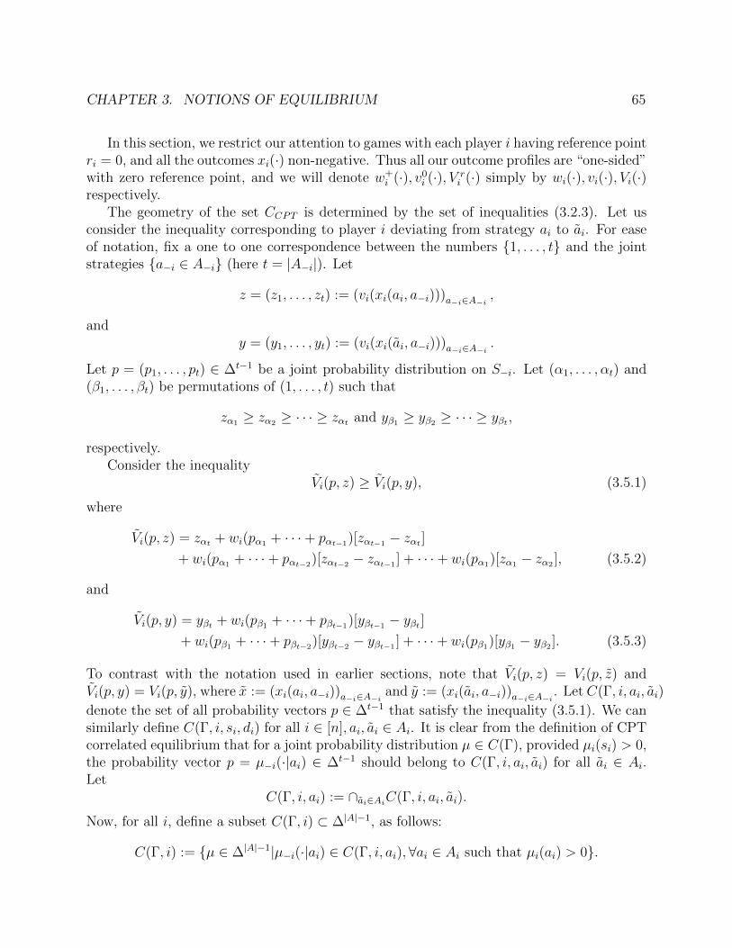
CHAPTER 3. NOTIONS OF EQUILIBRIUM 65
In this section, we restrict our attention to games with each player i having reference pointri = 0, and all the outcomes xi(·) non-negative. Thus all our outcome profiles are “one-sided”with zero reference point, and we will denote w+
i (·), v0i (·), V r
i (·) simply by wi(·), vi(·), Vi(·)respectively.
The geometry of the set CCPT is determined by the set of inequalities (3.2.3). Let usconsider the inequality corresponding to player i deviating from strategy ai to ai. For easeof notation, fix a one to one correspondence between the numbers 1, . . . , t and the jointstrategies a−i ∈ A−i (here t = |A−i|). Let
z = (z1, . . . , zt) := (vi(xi(ai, a−i)))a−i∈A−i ,
andy = (y1, . . . , yt) := (vi(xi(ai, a−i)))a−i∈A−i .
Let p = (p1, . . . , pt) ∈ ∆t−1 be a joint probability distribution on S−i. Let (α1, . . . , αt) and(β1, . . . , βt) be permutations of (1, . . . , t) such that
zα1 ≥ zα2 ≥ · · · ≥ zαt and yβ1 ≥ yβ2 ≥ · · · ≥ yβt ,
respectively.Consider the inequality
Vi(p, z) ≥ Vi(p, y), (3.5.1)
where
Vi(p, z) = zαt + wi(pα1 + · · ·+ pαt−1)[zαt−1 − zαt ]+ wi(pα1 + · · ·+ pαt−2)[zαt−2 − zαt−1 ] + · · ·+ wi(pα1)[zα1 − zα2 ], (3.5.2)
and
Vi(p, y) = yβt + wi(pβ1 + · · ·+ pβt−1)[yβt−1 − yβt ]+ wi(pβ1 + · · ·+ pβt−2)[yβt−2 − yβt−1 ] + · · ·+ wi(pβ1)[yβ1 − yβ2 ]. (3.5.3)
To contrast with the notation used in earlier sections, note that Vi(p, z) = Vi(p, z) andVi(p, y) = Vi(p, y), where x := (xi(ai, a−i))a−i∈A−i and y := (xi(ai, a−i))a−i∈A−i . Let C(Γ, i, ai, ai)
denote the set of all probability vectors p ∈ ∆t−1 that satisfy the inequality (3.5.1). We cansimilarly define C(Γ, i, si, di) for all i ∈ [n], ai, ai ∈ Ai. It is clear from the definition of CPTcorrelated equilibrium that for a joint probability distribution µ ∈ C(Γ), provided µi(si) > 0,the probability vector p = µ−i(·|ai) ∈ ∆t−1 should belong to C(Γ, i, ai, ai) for all ai ∈ Ai.Let
C(Γ, i, ai) := ∩ai∈AiC(Γ, i, ai, ai).
Now, for all i, define a subset C(Γ, i) ⊂ ∆|A|−1, as follows:
C(Γ, i) := µ ∈ ∆|A|−1|µ−i(·|ai) ∈ C(Γ, i, ai),∀ai ∈ Ai such that µi(ai) > 0.

CHAPTER 3. NOTIONS OF EQUILIBRIUM 66
Note that since C(Γ) is nonempty, the set C(Γ, i) is nonempty for each i. The set C(Γ, i)can be constructed from the sets C(Γ, i, ai), ai ∈ Ai as follows: let pai ∈ C(Γ, i, ai) forall ai ∈ Ai such that C(Γ, i, ai) 6= φ, let qi ∈ ∆|Ai|−1 be a probability distribution over Aisuch that qi(ai) = 0 for all ai ∈ Si such that C(Γ, i, ai) = ∅, and define a joint probabilitydistribution µ ∈ ∆|A|−1 by µ(ai, a−i) = qi(ai)p
ai(a−i) if C(Γ, i, ai) 6= φ and µ(ai, a−i) = 0otherwise. Then µ ∈ C(Γ, i), and for every µ ∈ C(Γ, i), the corresponding qi = µi for allai ∈ Ai and pai = µ−i(·|ai) for all ai ∈ Ai with C(Γ, i, ai) 6= φ. Further, it is clear that
C(Γ) = ∩i∈[n]C(Γ, i).
Thus the set C(Γ) is uniquely determined by the collection of sets
C(Γ, i, ai, ai), i ∈ [n], ai, ai ∈ Ai.
Lemma 3.5.1. In the above setting, the set C(Γ, i, ai, ai) is connected.
Proof. Suppose the permutations (α1, . . . , αt) and (β1, . . . , βt) can be chosen such that theyare equal. Let
lj := wi(
j∑k=1
pαk) = wi(
j∑k=1
pβk), for 1 ≤ j ≤ t. (3.5.4)
For every vector l = (l1, . . . , lt) ∈ Rt such that 0 ≤ l1 ≤ · · · ≤ lt = 1, there corresponds aunique probability vector p = (p1, . . . , pt) satisfying equations (3.5.4) and this mapping iscontinuous because wi(·) is a continuous strictly increasing function. Thus we have a one-to-one correspondence between probability vectors (p1, . . . , pt) and the vectors (l1, . . . , lt).
Inequality (3.5.1) can then be written as
ltzαt +t−1∑i=1
lt−i[zαt−i − zαt−i+1] ≥ ltyβt +
t−1∑i=1
lt−i[yβt−i − yβt−i+1]. (3.5.5)
Since this is linear in (l1, . . . , lt), the set of all vectors (l1, . . . , lt) satisfying inequal-ity (3.5.5) is a convex polytope. In particular, it is connected. Thus the set C(Γ, i, ai, ai) isalso connected.
Suppose now the permutations (α1, . . . , αt) and (β1, . . . , βt) cannot be chosen to be equal.Then there exists 1 ≤ j1, j2 ≤ t such that zj1 > zj2 and yj1 ≤ yj2 . If p ∈ C(Γ, i, ai, ai) suchthat pj2 > 0, then, by the stochastic dominance property, the following probability vectorq(ε), for all 0 ≤ ε ≤ 1, also belongs to C(Γ, i, ai, ai):
qj(ε) =
pj1 + (1− ε)pj2 if j = j1,
εpj2 if j = j2,
pj otherwise.

CHAPTER 3. NOTIONS OF EQUILIBRIUM 67
RED YELLOW GREENTOP 69, 10 61, 0 20, 10
CENTER 50, 0 60, 10 30, 0BOTTOM 101, 0 41, 10 0, 0
Table 3.1: Payoff matrix for the game in Section 3.6
Thus, from every vector p ∈ C(Γ, i, ai, ai), we have a path connecting it to a probabilityvector p′ ∈ C(Γ, i, ai, ai) such that p′j2 = 0. To show that C(Γ, i, ai, ai) is connected it isenough to show that the subset
C ′(Γ, i, ai, ai) = p′ ∈ C(Γ, i, ai, ai)|p′j2 = 0.
is connected. From (3.5.2) and (3.5.3), we can see that the CPT values of the prospects(p, z) and (p, y) with probability vector restricted to C ′(Γ, i, ai, ai) do not depend on theoutcomes zj2 and yj2 . If one can now choose permutations (α′1, . . . , α
′t−1) and (β′2, . . . , β
′t−1)
of 1, . . . , t\j2 such that
zα′1 ≥ zα′2 ≥ · · · ≥ zα′t−1and yβ′1 ≥ yβ′2 ≥ · · · ≥ yβ′t−1
,
then, as before, one can argue that the set C ′(i, si, di) is connected. If not, we can continue todecrease the support of the probability vectors under consideration. This process terminatessince our state space is finite.
Even though the sets C(Γ, i, ai, ai) are connected, their intersection might be discon-nected, as in the example given in the next section.
3.6 Example of a Game with Disconnected CPT
Correlated Equilibrium
Consider a 2 player Γ game with each player having three pure strategies: TOP, CENTER,BOTTOM for player 1 (row player) and RED, YELLOW, GREEN for player 2 (columnplayer), with the corresponding payoffs as shown in Table 3.1. For both the players, let vi(·)be the identity function. For the probability weight function wi(·) we employ the functionsuggested by Prelec [113], which, for i = 1, 2, is given by
wi(p) = exp−(− ln p)γi,
for some γi ∈ (0, 1]. We take γ1 = 0.5 and γ2 = 1. We will now see that the set C(Γ, 1,TOP)is disconnected. Fix the correspondence (R, Y,G) ↔ (RED, YELLOW, GREEN). The set

CHAPTER 3. NOTIONS OF EQUILIBRIUM 68
C(1,TOP,BOTTOM) consists of all probability vectors p = (pR, pY , pG) ∈ ∆2 satisfying thefollowing inequality:
20 + w1(pR + pY )[61− 20] + w1(pR)[69− 61]
≥ 0 + w1(pR + pY )[41− 0] + w1(pR)[101− 41].
This holds iff pR ≤ 0.40 (all the decimal numbers henceforth are correct up to two decimalpoints). Thus, we have
C(Γ, 1,TOP,BOTTOM) = p ∈ ∆2|pR ≤ 0.40.
The set C(Γ, 1,TOP,CENTER) consists of all probability vectors p = (pR, pY , pG) ∈ ∆2
satisfying the inequality
20 + w1(pR + pY )[61− 20] + w1(pR)[69− 61]
≥ 30 + w1(pR + pY )[50− 30] + w1(pY )[60− 50].
Rearranging, we get
21w1(1− pG)− 10w1(1− pR − pG) ≥ 10− 8w1(pR).
For each pR ∈ [0, 0.4], we solve the above inequality for pG. The set C(Γ, 1,TOP), as shownin Figure 3.1, is disconnected. One can check that
(0, ε, 1− ε) ∈ C(Γ, 1,CENTER) and (1− ε, ε, 0) ∈ C(Γ, 1,BOTTOM),
for ε ∈ [0, 0.20]. We cannot as yet conclude that the set C(Γ, 1) is disconnected, because ofthe existence of joint probability distributions µ with marginal distribution µ1(TOP) = 0.We now show that C(Γ, 2) cannot contain any distribution µ with µ1(TOP) = 0.
Fix the correspondence (T,C,B)↔ (TOP,CENTER,BOTTOM). A similar analysis forplayer 2 shows that
C(Γ, 2,RED) = p ∈ ∆2|pT ≥ 0.5,C(Γ, 2,YELLOW) = p ∈ ∆2|pT ≤ 0.5,C(Γ, 2,GREEN) = p ∈ ∆2|pT ≥ 0.5.
Suppose that there were µ ∈ C(Γ) with µ1(TOP) = 0. Then
µ(TOP,RED) = µ(TOP,YELLOW) = µ(TOP,GREEN) = 0,
and from the structure of the sets C(2,RED) and C(2,GREEN) we get
µ2(RED) = µ2(GREEN) = 0.

CHAPTER 3. NOTIONS OF EQUILIBRIUM 69
(1, 0, 0)
(0, 1, 0) (0, 0, 1)
pR = 0.40
Figure 3.1: Standard 2-simplex of probability vectors p = (pR, pY , pG). The shaded regionrepresents the set C(Γ, 1,TOP) and is disconnected.
Thus, the joint probability µ has support only on the strategy pairs (CENTER,YELLOW)and (BOTTOM,YELLOW). Thus, player 2 always plays strategy YELLOW and player 1mixes between CENTER and BOTTOM. However, given player 2 plays strategy YELLOW,player 1’s TOP strategy dominates strategies CENTER and BOTTOM. Hence such a jointprobability distribution is not possible. Thus there does not exist any distribution µ ∈ C(Γ)with µ1(TOP) = 0.
There is a possibility that one of the components of C(Γ, 1,TOP) could disappear in theintersection C(Γ, 1) ∩ C(2). However, this does not happen because both the distributionsµ, µ in Figure 3.2 belong to C(Γ) with µ−1(·|TOP) and µ−1(·|TOP) belonging to differentcomponents of C(Γ, 1,TOP).
3.7 Summary
Although the set of correlated equilibria under CPT has a more complicated geometry thana convex polytope, property (P), on the intersection of the Nash and correlated equilibriumsets, continues to hold. Property (P) is particularly relevant to the interactive learningproblem in game theory [50, 51, 60]. This raises the question of analyzing the interactivelearning problem under cumulative prospect theoretic preferences. We will get back to thisin Chapter 5. In this process, we will see that the notion of CPT correlated equilibriumneeds to be reconsidered.

CHAPTER 3. NOTIONS OF EQUILIBRIUM 70
RED YELLOW GREENTOP 0.4 0.1 0.5
CENTER 0 0.05 0.5BOTTOM 0.4 0.05 0
RED YELLOW GREENTOP 0.4 0 0.6
CENTER 0 0 0.6BOTTOM 0.4 0 0
Figure 3.2: Un-normalized distributions µ and µ.
In the next chapter, we will see another interesting phenomenon related to the notion ofNash equilibria when players have CPT preferences. We will rethink the reasoning behindthe definition of Nash equilibrium and discuss its implications to the definition of CPT Nashequilibrium. This will give rise to two novel notions of equilibrium that we call black-boxequilibrium.
Notes9A working paper [23] analyzes the set of correlated equilibria for 2x2 games. However, some of the results
in that paper are partially incorrect, and unfortunately, due to the untimely death of the author, they nevergot addressed. Our characterization is based on the ideas presented in that paper.
10Keskin defines CPT equilibrium assuming w+(·) = w−(·). However, the definition can be easily extendedto our general setting and the proof of existence goes through without difficulty.
11Even though the game Γ can be obtained as a limit of a sequence of games in G0, one cannot obtain, ingeneral, the set C(Γ) as a limit of the sets of correlated equilibria of the games in G0. This is because theset of correlated equilibria is only upper-semicontinuous as a function of the game.

71
Chapter 4
Black-Box Equilibrium:Reconsidering CPT Nash Equilibrium
4.1 Introduction
The independence axiom says that if lottery L1 is weakly preferred over lottery L2 by anagent (i.e. the agent wants lottery L1 at least as much as lottery L2), and L is some otherlottery, then, for 0 ≤ α ≤ 1, the combined lottery αL1 + (1 − α)L is weakly preferred overthe combined lottery αL2 + (1− α)L by that agent. A weakened form of the independenceaxiom, called betweenness, says that if lottery L1 is weakly preferred over lottery L2 (by anagent), then, for any 0 ≤ α ≤ 1, the mixed lottery L = αL1 +(1−α)L2 must lie between thelotteries L1 and L2 in preference. Betweenness implies that if an agent is indifferent betweenL1 and L2, then she is indifferent between any mixtures of them too. It is known thatindependence implies betweenness, but betweenness does not imply independence [34]. Asa result, EUT preferences, which are known to satisfy the independence axiom, also satisfybetweenness. CPT preferences, on the other hand, do not satisfy betweenness in general (seeExample 4.2.2). In fact, in Theorem 4.2.3, we show that CPT preferences satisfy betweennessif and only if they are EUT preferences (recall that EUT preferences are a special case ofCPT preferences).
Suppose in a non-cooperative game that given her beliefs about the other players, a playeris indifferent between two of her actions. Then according to EUT, she should be indifferentbetween any of the mixtures of these two actions. This facilitates the proof of the existenceof a Nash equilibrium in mixed actions for such games. However, with CPT preferences, theplayer could either prefer some mixture of these two actions over the individual actions orvice versa.
As a result, it is important to make a distinction in CPT regarding whether the playerscan actively randomize over their actions or not. One way to enable active randomizationis by assuming that each player has access to a randomizing device and the player can“commit” to the outcome of this randomization. The commitment assumption is necessary,

CHAPTER 4. BLACKBOX EQUILIBRIUM 72
as is evident from the following scenario (the gambles presented below appear in [112]). Aliceneeds to choose between the following two actions:
1. Action 1 results in a lottery L1 = (0.34, $20,000); (0.66, $0), i.e. she receives $20,000with probability 0.34 and nothing with probability 0.66.
2. Action 2 results in a lottery L2 = (0.17, $30,000); (0.83, $0).
(See Example 4.3.7 for an instance of a 2-player game with Alice and Bob, where Alicehas two actions that result in the above two lotteries.) Note that L1 is a less risky gamblewith a lower reward and L2 is a more risky gamble with a higher reward. Now consider acompound lottery L = 16/17L1 + 1/17L2. Substituting for the lotteries L1 and L2 we get Lin its reduced form to be
L = (0.01, $30,000); (0.32, $20,000); (0.67, $0).
In Example 4.2.1, we provide a CPT model for Alice’s preferences that result in lotteryL1 being preferred over lottery L2, whereas lottery L is preferred over lotteries L1 and L2.Roughly speaking, the underlying intuition is that Alice is risk-averse in general, and sheprefers lottery L1 over lottery L2. However, she over-weights the small 1% chance of getting$30,000 in L and finds it lucrative enough to make her prefer lottery L over both the lotteriesL1 and L2. Let us say Alice has a biased coin that she can use to implement the randomizedstrategy. Now, if Alice tossed the coin, and the outcome was to play action 2, then in theabsence of commitment, she will switch to action 1, since she prefers lottery L1 over lotteryL2. Commitment can be achieved, for example, by asking a trusted party to implementthe randomized strategy for her or use a device that would carry out the randomizationand implement the outcome without further consultation with Alice. Regardless of theimplementation mechanism, we will call such randomized strategies black-box strategies . Theabove problem of commitment is closely related to the problem of using non-EUT models indynamic decisions. For an interesting discussion on this topic, see Appendix C of [132] andthe references therein.
Traditionally, mixed actions have been considered from two viewpoints, especially inthe context of mixed action Nash equilibrium. According to the first viewpoint, these areconscious randomizations by the players – each player only knows her mixed action andnot its pure realization. The notion of black-box strategies captures this interpretationof mixed actions. According to the other viewpoint, players do not randomize, and eachplayer chooses some definite action, but the other players need not know which one, and themixture represents their uncertainty, i.e. their conjecture about her choice. Aumann andBrandenburger [8] establish mixed action Nash equilibrium as an equilibrium in conjecturesprovided they satisfy certain epistemic conditions regarding the common knowledge amongstthe players.
In the absence of the betweenness condition, these two viewpoints give rise to differentnotions of Nash equilibria. Throughout we assume that the player set and their correspond-ing action sets and payoff functions, as well as the rationality of each player, are common

CHAPTER 4. BLACKBOX EQUILIBRIUM 73
knowledge. A player is said to be rational if, given her beliefs and her preferences, she doesnot play any suboptimal strategy. Suppose each player plays a fixed action, and these fixedactions are common knowledge, then we get back the notion of pure Nash equilibrium (seeDefinition 4.3.2). If each player plays a fixed action, but the other players have mixed conjec-tures over her action, and these conjectures are common knowledge, then this gives us mixedaction Nash equilibrium (see Definition 4.3.4). This coincides with the notion of Nash equi-librium that we saw in Chapter 3. Now suppose each player can randomize over her actionsand hence implement a black-box strategy. If each player plays a fixed black-box strategyand these black-box strategies are common knowledge, then this gives rise to a new notionof equilibrium. We call it black-box strategy Nash equilibrium (see Definition 4.3.8). If eachplayer plays a fixed black-box strategy and the other players have mixed conjectures over herblack-box strategy, and these conjectures are common knowledge, then we get the notion ofmixed black-box strategy Nash equilibrium (see Definition 4.3.10). It should be noted that thenotion of mixed black-box strategy Nash equilibrium is identical to the notion of equilibriumin beliefs as defined in [37] when restricted to players having CPT preferences.12
In the setting of an n-player normal form game with real valued payoff functions, the pureNash equilibria do not depend on the specific CPT features of the players, i.e. the referencepoint, the value function and the two probability weighting functions, one for gains and onefor losses. Hence the traditional result on the lack of guarantee for the existence of a pureNash equilibrium continues to hold when players have CPT preferences. Keskin [74] provesthe existence of a mixed action Nash equilibrium for any finite game when players haveCPT preferences. In Example 4.3.9, we show that a finite game may not have any black-boxstrategy Nash equilibrium.13 On the other hand, in Theorem 4.3.12, we prove our mainresult that for any finite game with players having CPT preferences, there exists a mixedblack-box strategy Nash equilibrium. If the players have EUT preferences, then the notionsof black-box strategy Nash equilibrium and mixed black-box strategy Nash equilibrium areequivalent to the notion of mixed action Nash equilibrium (when interpreted appropriately;see the remark before Proposition 4.3.14; see also Figure 4.5).
The chapter is organized as follows. In Section 4.2, we describe the CPT setup andestablish that under this setup betweenness is equivalent to independence (Theorem 4.2.3).14
In Section 4.3, we describe an n-player non-cooperative game setup and define various notionsof Nash equilibrium in the absence of betweenness, in particular with CPT preferences. Wediscuss the questions concerning their existence and how these different notions of equilibriacompare with each other. In Section 5.6, we conclude with a table that summarizes theresults.
4.2 CPT and Betweenness
In this chapter, we assume that each person is associated with a fixed reference point r ∈ R,a value function v : R → R, and two probability weighting functions w± : [0, 1] → [0, 1], w+
for gains and w− for losses. The CPT value is evaluated as described in Section 1.3.

CHAPTER 4. BLACKBOX EQUILIBRIUM 74
We now define some axioms for preferences over lotteries. We are interested in “mixtures”of lotteries, i.e. lotteries with other lotteries as outcomes. Consider a (two-stage) compoundlottery K := (qj, Lj)1≤j≤t, where Lj = (pj, zj), 1 ≤ j ≤ t, are lotteries over real outcomesand qj is the chance of lottery Lj. We assume that
∑tj=1 q
j = 1. A two-stage compound
lottery can be reduced to a single-stage lottery by multiplying the probability vector pj
corresponding to the lottery Lj by qj for each j, 1 ≤ j ≤ t, and then adding the probabilitiesof identical outcomes across all the lotteries Lj, 1 ≤ j ≤ t. Let
∑tj=1 q
jLj denote the reducedlottery corresponding to the compound lottery K.
Let denote a preference relation over single-stage lotteries. We assume to be a weakorder, i.e. is transitive (if L1 L2 and L2 L3, then L1 L3) and complete (for allL1, L2, we have L1 L2 or L2 L1, where possibly both preferences hold). The additionalbinary relations ,∼,≺ and are derived from in the usual manner. A preference relation is a CPT preference relation if there exist CPT features (r, v, w±) such that L1 L2 iffV (L1) ≤ V (L2). Note that a CPT preference relation is a weak order. A preference relation satisfies independence if for any lotteries L1, L2 and L, and any constant 0 ≤ α ≤ 1,L1 L2 implies αL1 + (1 − α)L αL2 + (1 − α)L. A preference relation satisfiesbetweenness if for any lotteries L1 L2, we have L1 αL1 + (1 − α)L2 L2, for all0 ≤ α ≤ 1. A preference relation satisfies weak betweenness if for any lotteries L1 ∼ L2,we have L1 ∼ αL1 + (1− α)L2, for all 0 ≤ α ≤ 1.
Suppose a preference relation satisfies independence. Then L1 L2 implies
L1 = αL1 + (1− α)L1 αL1 + (1− α)L2 αL2 + (1− α)L2 = L2.
Thus, if a preference relation satisfies independence, then it satisfies betweenness. Also, if apreference relation satisfies betweenness, then it satisfies weak betweenness.
In the following example, we will provide CPT features for Alice so that her preferencesagree with those described in Section 4.1. This example also shows that cumulative prospecttheory can give rise to preferences that do not satisfy betweenness.
Example 4.2.1. Recall that Alice is faced with the following three lotteries:
L1 = (0.34, $20, 000); (0.66, $0),L2 = (0.17, $30, 000); (0.83, $0),
L = (0.01, $30, 000); (0.32, $20, 000); (0.67, $0).
Let r = 0 be the reference point of Alice. Thus all the outcomes lie in the gains domain. Letv(x) = x0.8 for x ≥ 0; Alice is risk-averse in the gains domain. Let the probability weightingfunction for gains be given by
w+(p) = exp−(− ln p)0.6,
a form suggested by Prelec [113] (see Figure 4.1). We won’t need the probability weightingfunction for losses. Direct computations show that V (L1) = 968.96, V (L2) = 932.29, and

CHAPTER 4. BLACKBOX EQUILIBRIUM 75
0 0.2 0.4 0.6 0.8 10
0.2
0.4
0.6
0.8
1
p
w+
(p)
AliceCharlie
Figure 4.1: The solid curve shows the probability weighting function for Alice from Exam-ple 4.2.1 and Example 4.3.7, and the dashed curve shows the probability weighting functionfor Charlie from Example 4.2.2.
V (L) = 1022.51 (all decimal numbers in this example are correct to two decimal places).Thus the preference behavior of Alice, as described in Section 4.1 (i.e., she prefers L1 overL2, but prefers L over L1 and L2), is consistent with CPT and can be modeled, for example,with the CPT features stated here.
The following example shows that CPT can give rise to preferences that do not satisfyweak betweenness (the lotteries and the CPT features presented below appear in [74]).
Example 4.2.2. Suppose Charlie has r = 0 as his reference point and v(x) = x as his valuefunction. Let his probability weighting function for gains be given by
w+(p) = exp−(− ln p)0.5.
(See Figure 4.1.) We won’t need the probability weighting function for losses since weconsider only outcomes in the gains domain in this example. Consider the lotteries L1 =(0.5, 2β); (0.5, 0) and L2 = (0.5, β + 1); (0.5, 1), where β = 1/w+(0.5) = 2.299 (alldecimal numbers in this example are correct to three decimal places). Direct computationsreveal that V (L1) = V (L2) = 2.000 > V (0.5L1 + 0.5L2) = 1.985.
Given a utility function u : R → R (assumed to be continuous and strictly increasing),the expected utility of a lottery L = (pk, zk)1≤k≤m is defined as U(L) :=
∑mk=1 pku(zk).
A preference relation is said to be an EUT preference relation if there exists a utilityfunction u such that L1 L2 iff U(L1) ≤ U(L2). Note that if the CPT probability weighting

CHAPTER 4. BLACKBOX EQUILIBRIUM 76
functions are linear, i.e. w±(p) = p for 0 ≤ p ≤ 1, then the CPT value of a lottery coincideswith the expected utility of that lottery with respect to the utility function u = v. It is wellknown that EUT preference relations satisfy independence and hence betweenness. Sev-eral generalizations of EUT have been obtained by weakening the independence axiom andassuming only betweenness, for example, weighted utility theory [32, 33], skew-symmetricbilinear utility [47, 18], implicit expected utility [40, 34] and disappointment aversion theory[55, 17]. The following theorem shows that in the restricted setting of CPT preferences,betweenness and independence are equivalent.
Theorem 4.2.3. If is a CPT preference relation, then the following are equivalent:
(i) is an EUT preference relation,
(ii) satisfies independence,
(iii) satisfies betweenness.
Wakker [131] considers rank-dependent utility (RDU) preferences [114], which is a specialcase of CPT preferences; RDU preferences are CPT preferences for which the probabilityweighting functions satisfy w+(p) = 1 − w−(1 − p) for all p ∈ [0, 1]. Wakker proves that,under RDU preferences , the probability weighting function w+ is linear if and only if satisfies betweenness. In fact, Wakker proves something more general. A preferencerelation is said to be quasi-concave (resp. quasi-convex) if for any lotteries L1, L2 andany constant 0 ≤ α ≤ 1, L1 L2 implies L1 αL1 + (1 − α)L2 (resp. L1 L2 impliesL1 αL1 + (1 − α)L2). Note that satisfies betweenness if it is both quasi-concave andquasi-convex. Wakker shows that, under RDU preferences, w+ is concave (resp. convex) ifand only if is quasi-concave (resp. quasi-convex).
Wakker proves this by defining a measure of convexity
λ[p, q] :=w+(p)/2 + w+(q)/2− w+(p/2 + q/2)
w+(p)− w+(q),
and showing that λ[p1, q2] + λ[p2, q2] ≥ 0, for any 0 ≤ p1 < q1 ≤ p2 < q2 ≤ 1, if satisfiesquasi-convexity by consideration of proper lotteries. A simple analytic proof is then usedto show that the above condition implies convexity of w+. Although Wakker’s proof canbe easily modified to account for general CPT preferences, we give an alternative proof inAppendix 4.B, where we show that the probability weighting functions satisfy[
w±(a2)− w±(b)] [w±(b)− w±(c1)
]=[w±(b)− w±(a1)
] [w±(c2)− w±(b)
],
for any 0 ≤ a1 < c1 < b < c2 < a2 ≤ 1 such that (a2 − b)(b − c1) = (b − a1)(c2 − b), if satisfies betweenness. We then solve this functional equation using the appropriate boundaryconditions and the continuity property of w± to show that w±(p) = p for p ∈ [0, 1].

CHAPTER 4. BLACKBOX EQUILIBRIUM 77
4.3 Equilibrium in Black-Box Strategies
We now consider an n-player non-cooperative game where the players have CPT preferences.We will discuss several notions of equilibrium for such a game and will contrast them.
Let Γ := (N, (Ai)i∈N , (xi)i∈N) denote a game, where N := 1, . . . , n is the set of players,Ai is the finite action set of player i, and xi : A → R is the payoff function for player i.Here A :=
∏iAi denotes the set of all action profiles a := (a1, . . . , an). Let A−i :=
∏i 6=j Aj
denote the set of action profiles a−i of all players except player i.
Definition 4.3.1. For any action profile a−i ∈ A−i of the opponents, we define the bestresponse action set of player i to be
Ai(a−i) := arg maxai∈Ai
xi(ai, a−i). (4.3.1)
Definition 4.3.2. An action profile a = (a1, . . . , an) is said to be a pure Nash equilibrium iffor each player i ∈ N , we have
ai ∈ Ai(a−i).
The notion of pure Nash equilibrium is the same whether the players have CPT pref-erences or EUT preferences because only deterministic lotteries, comprised of being offeredone outcome with probability 1, are considered in the framework of this notion. It is wellknown that for any given game Γ, a pure Nash equilibrium need not exist.
Let µ−i ∈ ∆(A−i) denote a belief of player i on the action profiles of her opponents.Given the belief µ−i of player i, if she decides to play action ai, then she will face the lottery(µ−i[a−i], xi(ai, a−i))a−i∈A−i .Definition 4.3.3. For any belief µ−i ∈ ∆(A−i), define the best response action set of player ias
Ai(µ−i) := arg maxai∈Ai
Vi
((µ−i[a−i], xi(ai, a−i))a−i∈A−i
). (4.3.2)
Note that this definition is consistent with the definition of the best response action setthat takes an action profile a−i of the opponents as its input (Definition 4.3.1), if we interpreta−i as the belief 1a−i ∈ ∆(A−i), since Ai(1a−i) = Ai(a−i).
Let σi ∈ ∆(Ai) denote a conjecture over the action of player i. Let σ := (σ1, . . . , σn)denote a profile of conjectures, and let σ−i := (σj)j 6=i denote the profile of conjectures for allplayers except player i. Let µ−i(σ−i) ∈ ∆(A−i) be the belief induced by conjectures σj, j 6= i,given by
µ−i(σ−i)[a−i] :=∏j 6=i
σj[a−i],
which is nothing but the product distribution induced by σ−i.
Definition 4.3.4. A conjecture profile σ = (σ1, . . . , σn) is said to be a mixed action Nashequilibrium if, for each player i, we have
ai ∈ Ai(µ−i(σ−i)), for all ai ∈ suppσi.

CHAPTER 4. BLACKBOX EQUILIBRIUM 78
In other words, the conjecture σi over the action of player i should assign positive prob-abilities to only optimal actions of player i, given her belief µ−i(σ−i).
It is well known that a mixed Nash equilibrium exists for every game with EUT players,see [99]. Keskin [74] generalizes the result of Nash [99] on the existence of a mixed actionNash equilibrium to the case when players have CPT preferences.
Let Bi := ∆(Ai) denote the set of all black-box strategies for player i with a typicalelement denoted by bi ∈ Bi. Recall that if player i implements a black-box strategy bi, thenwe interpret this as a trusted party other than the player sampling an action ai ∈ Ai fromthe distribution bi and playing action ai on behalf of player i. We assume the usual topologyon Bi. Let B :=
∏iBi and B−i :=
∏j 6=iBj with typical elements denoted by b and b−i,
respectively.Note that, although a conjecture σi and a black-box strategy bi are mathematically equiv-
alent, viz. they are elements of the same set Bi = ∆(Ai), they have different interpretations.We will call si ∈ ∆(Ai) a mixture of actions of player i when we want to be agnostic to whichinterpretation is being imposed. Let Si := ∆(Ai), S :=
∏i ∆(Ai) and S−i :=
∏j 6=i Si with
typical elements denoted by si, s and s−i, respectively. (Note that S 6= ∆(A) unless all butone player have singleton action sets.)
For any belief µ−i ∈ ∆(A−i) and any black-box strategy bi of player i, let µ(bi, µ−i) ∈∆(A) denote the product distribution given by
µ(bi, µ−i)[a] := bi[ai]µ−i[a−i].
Given the belief µ−i of player i, if she decides to implement the black-box strategy bi, thenshe will face the lottery µ(bi, µ−i)[a], xi(a))a∈A.
Definition 4.3.5. For any belief µ−i ∈ ∆(A−i), define the best response black-box strategy setof player i as
Bi(µ−i) := arg maxbi∈Bi
Vi((µ(bi, µ−i)[a], xi(a))a∈A
).
Lemma 4.3.6. For any belief µ−i, the set Bi(µ−i) is non-empty, and
co(Bi(µ−i)) = co(Bi(µ−i)).
See Appendix 4.C for proof.Let us compare the two concepts: the best response action set (Definition 4.3.3) and
the best response black-box strategy set (Definition 4.3.5). Even though both of them takethe belief µ−i of player i as input, the best response action set Ai(µ−i) outputs a collectionof actions of player i, whereas the best response black-box strategy set Bi(µ−i) outputs acollection of black-box strategies of player i, which are probability distributions over the setof actions ai ∈ Ai. If we interpret an action ai as the mixture 1ai ∈ Si = ∆(Ai), and ablack-box strategy bi as a mixture as well, then we can compare the two sets A (µ−i) andB(µ−i) as subsets of Si. The following example shows that, in general, the two sets can bedisjoint, and hence quite distinct.

CHAPTER 4. BLACKBOX EQUILIBRIUM 79
1 2 31 $20,000 $20,000 $02 $30,000 $0 $0
Figure 4.1: Payoff matrix for Alice in Example 4.3.7. Rows and columns correspond to Alice’sand Bob’s actions respectively. The amount in each cell corresponds to Alice’s payoff.
Example 4.3.7. We consider a 2-player game. Let Alice be player 1, with action set A1 =1, 2, and let Bob be player 2, with action set A2 = 1, 2, 3. Let the payoff functionfor Alice be as shown in Figure 4.1. Let µ−1 = (0.17, 0.17, 0.66) ∈ ∆(A−1) = ∆(A2)be the belief of Alice. Then, as considered in Section 4.1, Alice faces the lottery L1 =(0.34, $20, 000); (0.66, $0) if she plays action 1 and the lottery L2 = (0.17, $30, 000); (0.83, $0)if she plays action 2. We retain the CPT features for Alice, as in Example 4.2.1, viz.: r = 0,v(x) = x0.8 for x ≥ 0, and
w+(p) = exp−(− ln p)0.6.
We saw that V1(L1) = 968.96, V1(L2) = 932.29, and V (16/17L1 + 1/17L2) = 1022.51(all decimal numbers in this example are correct to two decimal places). Amongst all themixtures, the maximum CPT value is achieved at the unique mixture L∗ = α∗L1+(1−α∗)L2,where α∗ = 0.96; we have V1(L∗) = 1023.16. Thus, A1(µ−1) = 11 and B1(µ−1) =(α∗, 1− α∗).
For any black-box strategy profile b−i of the opponents, let µ−i(b−i) ∈ ∆(A−i) be theinduced belief given by
µ−i(b−i)[a−i] :=∏j 6=i
bj[a−i].
Definition 4.3.8. A black-box strategy profile b = (b1, . . . , bn) is said to be a black-box strategyNash equilibrium if, for each player i, we have
bi ∈ Bi(µ−i(b−i)).
If the players have EUT preferences, a conjecture profile σ = (σ1, . . . , σn) is a mixedaction Nash equilibrium if and only if the black-box strategy profile b = (b1, . . . , bn), wherebi = σi, for all i ∈ N , is a black-box strategy Nash equilibrium. Thus, under EUT, thenotion of a black-box strategy Nash equilibrium is equivalent to the notion of a mixed actionNash equilibrium, although there is still a conceptual difference between these two notionsbased on the interpretations for the mixtures of actions. Further, we have the existence of ablack-box strategy Nash equilibrium for any game when players have EUT preferences fromthe well-known result about the existence of a mixed action Nash equilibrium. The followingexample shows that, in general, a black-box strategy Nash equilibrium may not exist whenplayers have CPT preferences.

CHAPTER 4. BLACKBOX EQUILIBRIUM 80
0 10 4 01 3 1
0 10 0 11 1 0
Figure 4.2: Payoff matrices for the 2× 2 game in Example 4.3.9 (left matrix for player 1 andright matrix for player 2). The rows and the columns correspond to the actions of player 1and player 2, respectively, and the entries in the cell represent the corresponding payoffs.
Example 4.3.9. Consider a 2 × 2 game (i.e a 2-player game where each player has twoactions 0, 1) with the payoff matrices as shown in Figure 4.2. Let the reference points ber1 = r2 = 0. Let vi(·) be the identity function for i = 1, 2. Let the probability weightingfunctions for gains for the two players be given by
w+i (p) = exp−(− ln p)γi, for i = 1, 2,
where γ1 = 0.5 and γ2 = 1. We do not need the probability weighting functions for lossessince all the outcomes lie in the gains domain for both the players. Notice that player 2 hasEUT preferences since w+
2 (p) = p.Suppose player 1 and player 2 play black-box strategies (1− p, p) and (1− q, q), respec-
tively, where p, q ∈ [0, 1]. With an abuse of notation, we identify these black-box strategiesby p and q, respectively. The corresponding lottery faced by player 1 is given by
L1(p, q) := (µ[0, 0], 4); (µ[1, 0], 3); (µ[1, 1], 1); (µ[0, 1], 0),
where µ[0, 0] := (1 − p)(1 − q), µ[1, 0] := p(1 − q), µ[0, 1] := (1 − p)q, and µ[1, 1] := pq. By(1.3.8), the CPT value of the lottery faced by player 1 is given by
V1(L1(p, q)) := 4×[w+
1 (µ[0, 0])]
+ 3×[w+
1 (µ[0, 0] + µ[1, 0])− w+1 (µ[0, 0]))
]+ 1×
[w+
1 (µ[0, 0] + µ[1, 0] + µ[1, 1])− w+1 (µ[0, 0] + µ[1, 0])
].
The plot of the function V1(L1(p, q)) with respect to p, for q = 0.3 and q = 0.35, is shown inFigure 4.3. We observe that the best response black-box strategy set B1(µ−1(q)) of player 1to player 2’s black-box strategy q ∈ B2 satisfies the following: B1(µ−1(q)) = 0 for q < q∗,B1(µ−1(q)) = 0, p∗ for q = q∗, and B1(µ−1(q)) ⊂ [p∗, 1] for q > q∗, where p∗ = 0.996 andq∗ = 0.340 (here the numbers are correct to three decimal points). Further, B1(µ−1(q)) issingleton for q ∈ (q∗, 1] and the unique element in B1(µ−1(q)) increases monotonically withrespect to q from p∗ to 1 (see Figure 4.4). In particular, B1(µ−1(1)) = 1. The lotteryfaced by player 2 is given by
L2(p, q) := (µ[0, 0], 0); (µ[1, 0], 1); (µ[1, 1], 0); (µ[0, 1], 1),

CHAPTER 4. BLACKBOX EQUILIBRIUM 81
0 0.1 0.2 0.3 0.4 0.5 0.6 0.7 0.8 0.9 1
2.05
2.1
2.15
2.2
p
V1(L
1(p,q
))q = 0.3q = 0.35
Figure 4.3: The CPT value of player 1 in Example 4.3.9. Here, p and q denote the black-boxstrategies for player 1 and 2, respectively. Note the rise and sharp drop in the two curvesnear p = 1. For the curve for q = 0.3, the global maximum is attained at p = 0, whereas, forthe curve for q = 0.35, the global maximum is attained close to p = 1, specifically for somep ∈ [0.9, 1].
and the CPT value of player 2 for this lottery is given by V2(L2(p, q)) = p(1− q) + q(1− p).The best response black-box strategy set B2(µ−2(p)) of player 2 to player 1’s black-boxstrategy p ∈ B1 satisfies the following: B2(µ−2(p)) = 1 for p < 0.5, B2(µ−2(p)) = [0, 1]for p = 0.5, and B2(µ−2(p)) = 0 for p > 0.5. As a result, see Figure 4.4, there does notexist any (p′, q′) such that p′ ∈ B1(µ−1(q′)) and q′ ∈ B2(µ−2(p′)), and hence no black-boxstrategy Nash equilibrium exists for this game.
Let τi ∈ P(Bi) denote a conjecture over the black-box strategy of player i. This willinduce a conjecture σi(τi) ∈ ∆(Ai) over the action of player i, given by
σi(τi)[ai] = Eτibi[ai].
Given conjectures over black-box strategies (τj ∈ ∆(Bj), j 6= i), let σ−i(τ−i) := (σj(τj))j 6=i.
Definition 4.3.10. A profile of conjectures over black-box strategies τ = (τ1, . . . , τn) is saidto be a mixed black-box strategy Nash equilibrium if, for each player i, we have
bi ∈ Bi(µ−i(σ−i(τ−i))), for all bi ∈ supp τi.
Proposition 4.3.11. For a profile of conjectures σ∗ = (σ∗1, . . . , σ∗n), consider the condition
σ∗i ∈ co(Bi(µ−i(σ∗−i))), for all i. (4.3.3)
(i) If τ is a mixed black-box strategy Nash equilibrium, then the profile of conjectures σ∗,where σ∗i = σi(τi),∀i, satisfies (4.3.3).
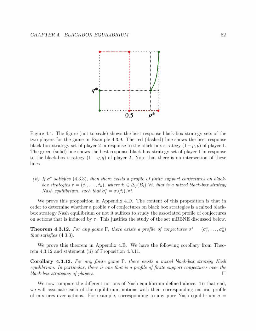
CHAPTER 4. BLACKBOX EQUILIBRIUM 82
Figure 4.4: The figure (not to scale) shows the best response black-box strategy sets of thetwo players for the game in Example 4.3.9. The red (dashed) line shows the best responseblack-box strategy set of player 2 in response to the black-box strategy (1− p, p) of player 1.The green (solid) line shows the best response black-box strategy set of player 1 in responseto the black-box strategy (1 − q, q) of player 2. Note that there is no intersection of theselines.
(ii) If σ∗ satisfies (4.3.3), then there exists a profile of finite support conjectures on black-box strategies τ = (τ1, . . . , τn), where τi ∈ ∆f (Bi), ∀i, that is a mixed black-box strategyNash equilibrium, such that σ∗i = σi(τi), ∀i.
We prove this proposition in Appendix 4.D. The content of this proposition is that inorder to determine whether a profile τ of conjectures on black box strategies is a mixed black-box strategy Nash equilibrium or not it suffices to study the associated profile of conjectureson actions that is induced by τ . This justifies the study of the set mBBNE discussed below.
Theorem 4.3.12. For any game Γ, there exists a profile of conjectures σ∗ = (σ∗1, . . . , σ∗n)
that satisfies (4.3.3).
We prove this theorem in Appendix 4.E. We have the following corollary from Theo-rem 4.3.12 and statement (ii) of Proposition 4.3.11.
Corollary 4.3.13. For any finite game Γ, there exists a mixed black-box strategy Nashequilibrium. In particular, there is one that is a profile of finite support conjectures over theblack-box strategies of players.
We now compare the different notions of Nash equilibrium defined above. To that end,we will associate each of the equilibrium notions with their corresponding natural profileof mixtures over actions. For example, corresponding to any pure Nash equilibrium a =

CHAPTER 4. BLACKBOX EQUILIBRIUM 83
(a1, . . . , an), assign the profile of mixtures over actions (1a1, . . . ,1an) ∈ S. Let pNE ⊂ Sdenote the set of all profiles of mixtures over actions that correspond to pure Nash equilibria.Let mNE ⊂ S denote the set of all mixed action Nash equilibria σ ∈ S. Let BBNE ⊂ Sdenote the set of all black-box strategy Nash equilibria b ∈ S. Corresponding to any mixedblack-box strategy Nash equilibrium τ = (τ1, . . . , τn), assign the profiles of mixtures overactions (σ1(τ1), . . . , σn(τn)) ∈ S, and let mBBNE ⊂ S denote the set of all such profiles.Note that each of the above subsets depends on the underlying game Γ and the CPT featuresof the players.
Proposition 4.3.14. For any fixed game Γ and CPT features of the players, we have
(i) pNE ⊂ mNE,
(ii) pNE ⊂ BBNE, and
(iii) BBNE ⊂ mBBNE.
Proof. The proof of statement (i) can be found in [74].For statement (ii), let (1a1, . . . ,1an) ∈ pNE. For a black-box strategy bi of player i,
the belief µ−i = 1a−i of player i gives rise to the lottery (bi[a′i], xi(a′i, a−i))a′i∈Ai . From thedefinition of CPT value (see Equation (1.3.8)), we observe that Vi((bi[a′i], xi(a′i, a−i))a′i∈Ai)is optimal as long as the probability distribution bi does not assign positive probability toany suboptimal outcome. Hence,
Bi(1a−i) = co(1a′i ∈ Si : a′i ∈ Ai(1a−i)).
In particular, 1ai ∈ Bi(1a−i), and hence (1a1, . . . ,1an) ∈ BBNE.Statement (iii) follows directly from the Definitions 4.3.8 and 4.3.10.
In the following, we show via examples that each of the labeled regions ((a)–(g)), inFigure 4.5, is non-empty in general.
Example 4.3.15. For each of the seven regions in Figure 4.5, we provide a 2 × 2 game withthe accompanying CPT features for the two players verifying that the corresponding regionis non-empty. Let the action sets be A1 = A2 = 0, 1. With an abuse of notation, letp, q ∈ [0, 1] denote the mixtures over actions for players 1 and 2, respectively, where p andq are the probabilities corresponding to action 1 for both the players. Thus, the set of allprofiles of mixtures over actions is S = (p, q) : p, q ∈ [0, 1]. Let L1(p, q) and L2(p, q) denotethe corresponding lotteries faced by the two players. (All decimal numbers in these examplesare correct to three decimal places.)
(a) Let both the players have EUT preferences with their utility functions given by the iden-tity functions ui(x) = x, for i = 1, 2. Let the payoff matrix be as shown in Figure 4.6a.Clearly, (p = 0, q = 0) ∈ pNE.

CHAPTER 4. BLACKBOX EQUILIBRIUM 84
SpNE
mNE
BBNEBBNE
mBBNE
ab
c
d
e
fg
Figure 4.5: Venn diagram depicting the different notions of equilibrium as subsets of theset S =
∏i ∆(Ai). The sets marked pNE,mNE,BBNE, and mBBNE represent the sets of
pure Nash equilibria, mixed action Nash equilibria, black-box strategy Nash equilibria, andmixed black-box strategy Nash equilibria, respectively. Examples are given in the body ofthe text of CPT games lying in each of the indicated regions (a) through (g).
(b) Let ri = 0, vi(x) = x, for i = 1, 2. Let w+1 (p) = p0.5 and w+
2 (p) = p, for p ∈ [0, 1]. Letthe payoff matrix be as shown in Figure 4.6b, where β := 1/w+
1 (0.5) = 1.414. We have
L1(p, q) = ((1− p)(1− q), 2β); (p(1− q), β + 1); (pq, 1); ((1− p)q, 0).
The way β is defined, we get V1(L1(0, 0.5)) = V1(L1(1, 0.5)) = 2. Also, observe thatV2(L2(0.5, 0)) = V2(L2(0.5, q)) = V2(L2(0.5, 1)),∀q ∈ [0, 1]. With these observations, weget that (0.5, 0.5) ∈ mNE. We have, arg maxp∈[0,1] V1(L1(p, 0.5)) = p′, where p′ = 0.707(see Figure 4.7). Hence 0.5 /∈ co(B1(µ−1(0.5))) and (0.5, 0.5) /∈ mBBNE.
(c) Let the CPT features for both the players be as in (b). Let the payoff matrix be asshown in Figure 4.6c, where β := 1/w+
1 (0.5) = 1.414 and γ = (1−p′)/p′ (here p′ = 0.707as in (b)). As observed in (b), B1(µ−1(0.5)) = p′. From the definition of γ, we seethat player 2 is indifferent between her two actions, given her belief p′ over player 1’sactions. Thus (p′, 0.5) ∈ (mNE ∩ BBNE)\pNE.
(d) Let ri = 0, vi(x) = x, for i = 1, 2. Let w−1 (p) = p0.5, w+2 (p) = p. Let the payoff
matrix be as shown in Figure 4.6d, where β := 1/w−1 (0.5) = 1.414. Note that thepayoffs for player 1 are negations of her payoffs in (b), and her probability weighing

CHAPTER 4. BLACKBOX EQUILIBRIUM 85
function for losses is same as her probability weighing function for gains in (b). Thusher CPT value function V1(L1(p, q)) is the negation of her CPT value function in (b).In particular, we have V1(L1(0, 0.5)) = V1(L1(1, 0.5)) > V1(L1(p, 0.5)) for all p ∈ (0, 1).Thus, 0.5 ∈ co(B1(µ−1(0.5))), but 0.5 /∈ B1(µ−1(0.5)). The payoffs and CPT featuresof player 2 are same as in (b). Thus, (0.5, 0.5) ∈ (mNE ∩mBBNE)\BBNE.
(e) Let the CPT features for both the players be as in (b). Let the payoff matrix be asshown in Figure 4.6e, where β := 1/w+
1 (0.5) = 1.414, ε = 0.1, and γ := (1 − p)/p;here p = 0.582 is the unique maximizer of V1(L1(p, 0.5)) (see Figure 4.8). We haveV1(L1(0, 0.5)) = 2.071 > 2 = V1(L1(1, 0.5)) and arg maxp V1(L1(p, 0.5)) = p withV1(L1(p, 0.5)) = 2.125. From the definition of γ, we see that player 2 is indifferentbetween her two actions, given her belief p over player 1’s actions. Thus, (p, 0.5) ∈BBNE\mNE.
(f) Let the CPT features be as in Example 4.3.9. Let p∗ = 0.996 and q∗ = 0.340 be the sameas in Example 4.3.9. Let the payoff matrix be as shown in Figure 4.6f. Note that thepayoffs for both the players are the same as in Example 4.3.9. Recall B1(µ−1(q)) = 0for q < q∗, B1(µ−1(q)) = 0, p∗ for q = q∗, and B1(µ−1(q)) ⊂ [p∗, 1] for q > q∗, andhence 0.5 ∈ co(B1(µ−1(q∗))) and 0.5 /∈ B1(µ−1(q∗)). Further, from the definition of γ,we have V2(L2(0.5, 0)) = V2(L2(0.5, q)) = V2(L2(0.5, 1)), ∀q ∈ [0, 1]. Hence, (0.5, q∗) ∈mBBNE\(mNE ∩ BBNE).
(g) Finally, if we let the players have EUT preferences and the payoffs as in (a), then(1, 0) /∈ (mNE ∪mBBNE).
4.4 Summary
In the study of non-cooperative game theory from a decision-theoretic viewpoint, it is im-portant to distinguish between two types of randomization:
1. conscious randomizations implemented by the players, and
2. randomizations in conjectures resulting from the beliefs held by the other players aboutthe behavior of a given player.
This difference becomes evident when the preferences of the players over lotteries do not sat-isfy betweenness, a weakened form of independence property. We considered n-player normalform games where players have CPT preferences, an important example of preference relationthat does not satisfy betweenness. This gives rise to four types of Nash equilibrium notions,depending on the different types of randomizations. We defined these different notions ofequilibrium and discussed the question of their existence. The results are summarized inTable 4.1.

CHAPTER 4. BLACKBOX EQUILIBRIUM 86
0 10 1, 1 0, 01 0, 0 0, 0
(a) pNE
0 10 2β, 0 0, 11 β + 1, 1 1, 0
(b) mNE\mBBNE
0 10 2β, 0 0, 11 β + 1, γ 1, 0
(c) (mNE ∩ BBNE)\pNE
0 10 −2β, 0 0, 11 −(β + 1), 1 −1, 0
(d) (mNE ∩mBBNE)\BBNE
0 10 2β + ε, 0 0, 11 β + 1, γ 1, 0
(e) BBNE\mNE
0 10 4, 0 0, 11 3, 1 1, 0
(f) mBBNE\(mNE ∪ BBNE)
Figure 4.6: Payoff matrices for the 2 × 2 games in Example 4.3.15. The rows and thecolumns correspond to the actions of player 1 and player 2, respectively. In each cell, theleft and right entries correspond to player 1 and player 2, respectively. The labels indicatethe corresponding regions in Figure 4.5. The game matrix for the example corresponding toregion (g) is the same as that for the one corresponding to region (a).
0 0.2 0.4 0.6 0.8 12
2.02
2.04
2.06
2.08
p
V1(L
1(p,0.5
))
Figure 4.7: The CPT value function forplayer 1 in Example 4.3.15(b), when q =0.5 is the mixture of actions of player 2.
0 0.2 0.4 0.6 0.8 12
2.05
2.1
p
V1(L
1(p,0.5
))
Figure 4.8: The CPT value function forplayer 1 in Example 4.3.15(e), when q =0.5 is the mixture of actions of player 2.

CHAPTER 4. BLACKBOX EQUILIBRIUM 87
Type of Nashequilibrium
Strategies Conjectures Always exists
Pure Nash equilibrium Pureactions
Exact conjectures No
Mixed action Nashequilibrium
Pureactions
Mixed conjectures Yes [74]
Black-box strategy Nashequilibrium
Black boxstrategies
Exact conjectures No (Exam-ple 4.3.9)
Mixed black-boxstrategy Nashequilibrium
Black boxstrategies
Mixed conjectures Yes (Theo-rem 4.3.12)
Table 4.1: Different types of Nash equilibrium when players have CPT preferences.
Appendix
4.A Proof of Theorem 4.2.3
Proof. Let the CPT preference relation be given by (r, v, w±). Since an EUT preferencerelation satisfies independence, we get that (i) implies (ii). Since betweenness is a weakercondition than independence, we get that (ii) implies (iii). We will now show that if satisfies betweenness, then the probability weighting functions are linear, i.e. w±(p) = p for0 ≤ p ≤ 1. This will imply that is an EUT preference relation with utility function u = v,and hence complete the proof.
Assume that the CPT preference relation satisfies betweenness. Consider a lotteryA := (p1, z1), (p2, z2), (1−p1−p2, r) such that z1 ≥ z2 ≥ r, p1 ≥ 0, p2 > 0 and p1 +p2 ≤ 1.By (1.3.9), we have
V (A) = δ1w+(P1) + δ2w
+(P2),
where δ1 := v(z1) − v(z2), δ2 := v(z2), P1 := p1 and P2 := p1 + p2. Let lottery B :=(q1, z1), (q2, z2), (1−q1−q2, r) be such that q1, q2 ≥ 0, Q1 := q1 > p1, and Q2 := q1+q2 < P2.By (1.3.9), we have
V (B) = δ1w+(Q1) + δ2w
+(Q2).
If z1, z2, p1, p2, q1 and q2 are such that
δ1
δ2
=w+(P2)− w+(Q2)
w+(Q1)− w+(P1), (4.A.1)

CHAPTER 4. BLACKBOX EQUILIBRIUM 88
then V (A) = V (B) and, by betweenness, for any 0 ≤ α ≤ 1 we have V (A) = V (B) =V (αA+ (1− α)B), i.e.
δ1w+(Q1) + δ2w
+(Q2) = δ1w+(αP1 + (1− α)Q1) + δ2w
+(αP2 + (1− α)Q2).
Using (4.A.1) we get[w+(P2)− w+(Q2)
] [w+(Q1)− w+(αP1 + (1− α)Q1))
]=[w+(Q1)− w+(P1)
] [w+(αP2 + (1− α)Q2)− w+(Q2)
]. (4.A.2)
Given any 0 ≤ P1 < Q1 ≤ Q2 < P2 ≤ 1, there exist z1 and z2 such that (4.A.1) holds.Indeed, take any δ > 0 belonging to the range of the function v. This exists because v(r) = 0and v is a strictly increasing function. Since w+ is a strictly increasing function, we have
κ :=w+(P2)− w+(Q2)
w+(Q1)− w+(P1)> 0.
Take z2 = v−1(δ/(1 + κ)) and z1 = v−1(δ). These are well defined because v is assumedto be continuous and strictly increasing, and δ belongs to its range. Hence z1 > z2 > r asrequired. Thus (4.A.2) holds for any 0 ≤ P1 < Q1 ≤ Q2 < P2 ≤ 1. In particular, whenQ1 = Q2, we have[
w+(P2)− w+(Q)] [w+(Q)− w+(R1)
]=[w+(Q)− w+(P1)
] [w+(R2)− w+(Q)
],
where Q := Q1 = Q2, R1 := αP1 + (1 − α)Q and R2 := αP2 + (1 − α)Q. Equivalently, forany 0 ≤ a1 < c1 < b < c2 < a2 ≤ 1 such that (a2 − b)(b− c1) = (b− a1)(c2 − b), we have[
w+(a2)− w+(b)] [w+(b)− w+(c1)
]=[w+(b)− w+(a1)
] [w+(c2)− w+(b)
].
In Lemma 4.B.1, we prove that the above condition implies w+(p) = p, for 0 ≤ p ≤ 1.Similarly, we can show that w−(p) = p, for 0 ≤ p ≤ 1. This completes the proof.
4.B An Interesting Functional Equation
Lemma 4.B.1. Let w : [0, 1] → [0, 1] be a continuous, strictly increasing function suchthat w(0) = 0 and w(1) = 1. For any 0 ≤ a1 < c1 < b < c2 < a2 ≤ 1 such that(a2 − b)(b− c1) = (b− a1)(c2 − b), let
[w(a2)− w(b)] [w(b)− w(c1)] = [w(b)− w(a1)] [w(c2)− w(b)] . (4.B.1)
Then w(p) = p for all p ∈ [0, 1].

CHAPTER 4. BLACKBOX EQUILIBRIUM 89
Proof. Taking a1 = 0, c1 = 1/4, b = 1/2, c2 = 3/4 and a2 = 1 in (4.B.1) we get,
[1− w(1/2)] [w(1/2)− w(1/4)] = [w(1/2)] [w(3/4)− w(1/2)] ,
and hence,
w(3/4) =w(1/2) + w(1/2)w(1/4)− w(1/4)
w(1/2).
Note that w(1/2) > 0. Taking a1 = 0, c1 = 1/4, b = 1/3, c2 = 1/2 and a2 = 1 in (4.B.1) weget,
[1− w(1/3)] [w(1/3)− w(1/4)] = [w(1/3)] [w(1/2)− w(1/3)] ,
and hence,
w(1/3) =w(1/4)
1− w(1/2) + w(1/4).
Note that 1−w(1/2) +w(1/4) > 1−w(1/2) > 0. Taking a1 = 0, c1 = 1/3, b = 1/2, c2 = 2/3and a2 = 1 in (4.B.1) we get,
[1− w(1/2)] [w(1/2)− w(1/3)] = [w(1/2)] [w(2/3)− w(1/2)] ,
and substituting for w(1/3) we get,
w(2/3) =w(1/2)− w(1/2)2 + 2w(1/2)w(1/4)− w(1/4)
w(1/2)− w(1/2)2 + w(1/2)w(1/4).
Note that
w(1/2)− w(1/2)2 + w(1/2)w(1/4) = w(1/2)[1− w(1/2) + w(1/4)] > 0.
Taking a1 = 0, c1 = 1/2, b = 2/3, c2 = 3/4 and a2 = 1 in (4.B.1) we get,
[1− w(2/3)] [w(2/3)− w(1/2)] = [w(2/3)] [w(3/4)− w(2/3)] .
Simplifying we get,
w(2/3)− w(2/3)w(3/4) = w(1/2)− w(1/2)w(2/3),
Substituting for w(2/3) and w(3/4) we get,[w(1/2)− w(1/2)2 + 2w(1/2)w(1/4)− w(1/4)
w(1/2)− w(1/2)2 + w(1/2)w(1/4)
] [w(1/4)− w(1/2)w(1/4)
w(1/2)
]= w(1/2)
[w(1/4)− w(1/2)w(1/4)
w(1/2)− w(1/2)2 + w(1/2)w(1/4)
].

CHAPTER 4. BLACKBOX EQUILIBRIUM 90
Since w(1/4)− w(1/2)w(1/4) > 0 and w(1/2)− w(1/2)2 + w(1/2)w(1/4) > 0, we get
w(1/2)− w(1/4) = 2w(1/2)[w(1/2)− w(1/4)].
Since w(1/2)− w(1/4) > 0, we get w(1/2) = 1/2.For any fixed 0 ≤ x < y ≤ 1, let
w′(p′) :=w(p′(y − x) + x)− w(x)
w(y)− w(x), for all 0 ≤ p′ ≤ 1.
Note that w′ : [0, 1]→ [0, 1] is a continuous, strictly increasing function with w′(0) = 0 andw′(1) = 1. Further, if 0 ≤ a′1 < c′1 < b′ < c′2 < a′2 ≤ 1 are such that (a′2 − b′)(b′ − c′1) =(b′ − a′1)(c′2 − b′), then
[w′(a′2)− w′(b′)] [w′(b′)− w′(c′1)] = [w′(b′)− w′(a′1)] [w′(c′2)− w′(b′)] .
Thus w′(1/2) = 1/2 and hence w ((x+ y)/2) = (w(x) + w(y))/2. Using this repeatedly weget w(k/2t) = k/2t, for 0 ≤ k ≤ 2t, t = 1, 2, . . . . Continuity of w then implies w(p) = p, forall p ∈ [0, 1].
4.C Proof of Lemma 4.3.6
Proof. For a lottery L = (p, z), where z = (zk)1≤k≤m is the outcome profile, and (pk)1≤k≤mis the probability vector, the function Vi(p, z) is continuous with respect to p ∈ ∆m−1 [74].Thus, Vi((µ(bi, µ−i)[a], xi(a))a∈A) is a function continuous with respect to bi ∈ Bi, andhence Bi(µ−i) is a non-empty closed subset of the compact space Bi. Since the convex hullof a compact subset of a Euclidean space is compact, the set co(Bi(µ−i)) is closed. Thiscompletes the proof.
4.D Proof of Proposition 4.3.11
Proof. Suppose τ is a mixed black-box strategy Nash equilibrium. Let σ∗i = σi(τi). Then,for all bi ∈ supp τi, we have bi ∈ Bi(µ−i(σ
∗−i)), and hence σ∗i ∈ co(Bi(µ−i(σ
∗−i))). This proves
statement (i).For statement (ii), suppose σ∗ satisfies condition (4.3.3). In fact, by Lemma 4.3.6 we
have, σ∗i ∈ co(Bi(µ−i(σ∗−i))) ⊂ ∆(Ai), and by Caratheodory’s theorem, σ∗i is a convex
combination of at most |Ai| elements in Bi(µ−i(σ∗−i)). Hence, we can construct a mixed
black-box strategy Nash equilibrium τ such that τi ∈ ∆f (Bi) and σ∗i = σi(τi),∀i.
4.E Proof of Theorem 4.3.12
Proof. The idea is to use the Kakutani fixed-point theorem, as in the proof of the existenceof mixed action Nash equilibrium [100]. Assume the usual topology on Si, for each i, and

CHAPTER 4. BLACKBOX EQUILIBRIUM 91
let S have the corresponding product topology. The set S is a non-empty compact convexsubset of the Euclidean space
∏i R|Ai|. Let K(σ) be the set-valued function given by
K(σ) :=∏i
co(Bi(µ−i(σ−i))),
for all σ ∈ S. Since co(Bi(µ−i(σ−i))) is non-empty and convex for each i (Lemma 4.3.6),the function K(σ) is non-empty and convex for any σ ∈ S. We now show that the functionK(·) has a closed graph. Let σt∞t=1 and st∞t=1 be two sequences in S that converge to σand s, respectively, and let st ∈ K(σt) for all t. It is enough to show that s ∈ K(σ). For allsi ∈ Si, σ−i ∈ S−i, let
Vi(si, σ−i) := supτi∈P(Bi),Eτibi=si
EτiVi ((µ(bi, µ−i(σ−i))[a], xi(a))a∈A) .
Since the product distribution µ(bi, µ−i(σ−i)) is jointly continuous in bi and σ−i, and, asnoted earlier, Vi(p, z) is continuous with respect to the probability vector p, for any fixedoutcome profile z, the function Vi (µ(bi, µ−i(σ−i))[a], xi(a)a∈A) is jointly continuous in biand σ−i. This implies that the function Vi(si, σ−i) is jointly continuous in si and σ−i (seeAppendix 4.F). From the definition of Vi, it follows that
maxsi∈∆(Ai)
Vi(si, σ−i) = maxbi∈Bi
Vi ((µ(bi, µ−i(σ−i))[a], xi(a))a∈A) .
Indeed, the maximum on the left-hand side is well-defined since ∆(Ai) is a compact spaceand Vi(·, σ−i) is a continuous function. The maximum on the right-hand side is well-definedand the maximum is achieved by all bi ∈ Bi(µ−i(σ−i)) (Lemma 4.3.6). Hence,
arg maxsi∈∆(Ai)
Vi(si, σ−i) = co(Bi(µ−i(σ−i))).
Since sti ∈ co(Bi(µ−i(σt−i))), for all t, we have
Vi(sti, σ
t−i) ≥ Vi(si, σ
t−i), for all si ∈ Si.
Since Vi(si, σ−i) is jointly continuous in si and σ−i, we get
Vi(si, σ−i) ≥ Vi(si, σ−i), for all si ∈ Si.
Hence we have si ∈ co(Bi(µ−i(σt−i))). This shows that the function K(·) has a closed graph.
By the Kakutani fixed-point theorem, there exists σ∗ such that σ∗ ∈ K(σ∗), i.e. σ∗ satisfiescondition (4.3.3) [69]. This completes the proof.
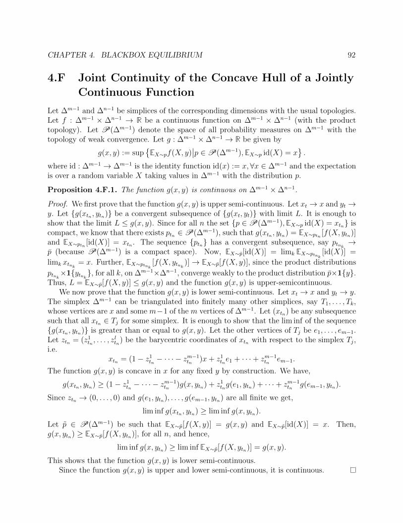
CHAPTER 4. BLACKBOX EQUILIBRIUM 92
4.F Joint Continuity of the Concave Hull of a Jointly
Continuous Function
Let ∆m−1 and ∆n−1 be simplices of the corresponding dimensions with the usual topologies.Let f : ∆m−1 × ∆n−1 → R be a continuous function on ∆m−1 × ∆n−1 (with the producttopology). Let P(∆m−1) denote the space of all probability measures on ∆m−1 with thetopology of weak convergence. Let g : ∆m−1 ×∆n−1 → R be given by
g(x, y) := sup
EX∼pf(X, y)∣∣p ∈P(∆m−1),EX∼p id(X) = x
.
where id : ∆m−1 → ∆m−1 is the identity function id(x) := x, ∀x ∈ ∆m−1 and the expectationis over a random variable X taking values in ∆m−1 with the distribution p.
Proposition 4.F.1. The function g(x, y) is continuous on ∆m−1 ×∆n−1.
Proof. We first prove that the function g(x, y) is upper semi-continuous. Let xt → x and yt →y. Let g(xtn , ytn) be a convergent subsequence of g(xt, yt) with limit L. It is enough toshow that the limit L ≤ g(x, y). Since for all n the set p ∈P(∆m−1),EX∼p id(X) = xtn iscompact, we know that there exists ptn ∈P(∆m−1), such that g(xtn , ytn) = EX∼ptn [f(X, ytn)]and EX∼ptn [id(X)] = xtn . The sequence ptn has a convergent subsequence, say ptnk →p (because P(∆m−1) is a compact space). Now, EX∼p[id(X)] = limk EX∼ptnk [id(X)] =
limk xtnk = x. Further, EX∼ptnk [f(X, ytnk )]→ EX∼p[f(X, y)], since the product distributions
ptnk×1ytnk, for all k, on ∆m−1×∆n−1, converge weakly to the product distribution p×1y.Thus, L = EX∼p[f(X, y)] ≤ g(x, y) and the function g(x, y) is upper-semicontinuous.
We now prove that the function g(x, y) is lower semi-continuous. Let xt → x and yt → y.The simplex ∆m−1 can be triangulated into finitely many other simplices, say T1, . . . , Tk,whose vertices are x and some m−1 of the m vertices of ∆m−1. Let (xtn) be any subsequencesuch that all xtn ∈ Tj for some simplex. It is enough to show that the lim inf of the sequenceg(xtn , ytn) is greater than or equal to g(x, y). Let the other vertices of Tj be e1, . . . , em−1.Let ztn = (z1
tn , . . . , zltn) be the barycentric coordinates of xtn with respect to the simplex Tj,
i.e.xtn = (1− z1
tn − · · · − zm−1tn )x+ z1
tne1 + · · ·+ zm−1tn em−1.
The function g(x, y) is concave in x for any fixed y by construction. We have,
g(xtn , ytn) ≥ (1− z1tn − · · · − z
m−1tn )g(x, ytn) + z1
tng(e1, ytn) + · · ·+ zm−1tn g(em−1, ytn).
Since ztn → (0, . . . , 0) and g(e1, ytn), . . . , g(em−1, ytn) are all finite we get,
lim inf g(xtn , ytn) ≥ lim inf g(x, ytn).
Let p ∈ P(∆m−1) be such that EX∼p[f(X, y)] = g(x, y) and EX∼p[id(X)] = x. Then,g(x, ytn) ≥ EX∼p[f(X, ytn)], for all n, and hence,
lim inf g(x, ytn) ≥ lim inf EX∼p[f(X, ytn)] = g(x, y).
This shows that the function g(x, y) is lower semi-continuous.Since the function g(x, y) is upper and lower semi-continuous, it is continuous.

CHAPTER 4. BLACKBOX EQUILIBRIUM 93
Notes12 Crawford [37] defines the notion of equilibrium in beliefs for 2-player games, but, as noted by Crawford,
it can be easily extended to games with more than 2 players.13 For the setting of 2-player games, this follows from the result of Crawford [37] on the existence of
equilibrium in beliefs. A technical complex analysis argument is required to extend this result to more than2 players. It appears that Crawford was aware of this (see footnote 9 in [37]). We provide an independentproof in Section 4.3 for the sake of completeness.
14 A similar result was proved by Wakker [131] in the setting of rank-dependent utility (RDU) preferences[114], which is a special case of CPT preferences. See the discussion following Theorem 4.2.3 for more onthis.

94
Chapter 5
Mediated Correlated Equilibrium:Reconsidering CPT CorrelatedEquilibrium
5.1 Introduction
In the previous two chapters we took the neoclassical economics viewpoint of game theorythat attempts to explain an equilibrium as a self-evident outcome of the optimal behaviorof the participating players, assuming them to be rational. An alternative approach, calledlearning in games, is concerned with justifying equilibrium behavior via a dynamic processwhere the players learn from the past play and observations from the environment, and adaptaccordingly [7, 52, 136]. In this chapter, we will be concerned with this alternative approach.Along the process, we will naturally come up with a modified version of the notion of CPTcorrelated equilibrium that will prove to be more appropriate in the settings of learning ingames as well as mechanism design, which we consider in more detail in the next chapter.
It becomes even more important to consider non-EUT behavior in the theory of learningin games. For example, in a repeated game, Hart [59] argues that players tend to use simpleprocedures like regret minimization. A player i is said to have no regret15 if, for each pair ofher actions ai, ai, she does not regret not having played action ai whenever she played actionai. Such regrets can simply be computed as the difference in the average payoffs receivedby the player from playing action ai instead of action ai, assuming the opponents stick totheir actions. While evaluating such regrets in the real world, however, players who aremodeled as evaluating lotteries according to CPT preferences are likely to exhibit differentkinds of learning behavior than that exhibited by EUT players. The proposed model in thischapter is an attempt to handle these systematic deviations in learning, anticipated from theempirically observed behavioral features exhibited by human agents, as captured by CPT.We pose the following question: How do the predictions of the theory of learning in gameschange if the players behave according to CPT?
CHAPTER 5. MEDIATED CORRELATED EQUILIBRIUM 95
For a repeated game, Foster and Vohra [49] describe a procedure based on calibratedlearning that guarantees the convergence of the empirical distribution of action play to the setof correlated equilibria, when players behave according to EUT. In Section 5.2, we formulatean analog for their procedure when players behave according to CPT. In Example 5.2.1, wedescribe a game for which the set of all CPT correlated equilibria is non-convex and we showthat the empirical distribution of action play does not converge to this set.
We then define an extension of the set of CPT correlated equilibria and establish theconvergence of the empirical distribution of action play to this extended set. It turns out thatthis extension has a nice game-theoretic interpretation, obtained by allowing the mediatorto send any private signal (instead of restricting her to send a signal corresponding to someaction). We formally define this setup in Section 5.3, and call it a mediated game. Myerson[91] has considered a further generalization in which each player i first reports her type froma finite set Ti. The mediator collects the reports from all the players and then sends eachone of them a private signal from a finite set Bi. The mediator is characterized by a ruleψ :
∏i Ti → ∆(
∏iBi) that maps each type profile to a probability distribution on the
set of signal profiles from which it samples the private signals to be sent. Based on herreceived signal, each player chooses her action. These are called games with communication.The type sets (Ti)
ni=1, the signal sets (Bi)
ni=1, and the mediator rule ψ together are said
to comprise a communication system. Under EUT, the set of all correlated equilibria of agame is characterized as the union, over all possible communication systems, of the sets ofjoint distributions on the action profiles of all players arising from all the Nash equilibriafor the corresponding game with communication (for a detailed exposition, see Chapter 6 in[89]). This is sometimes referred to as the Bayes-Nash revelation principle, or simply therevelation principle. Since a mediated game is a specific type of game with communication,characterized by players not reporting their type, or equivalently by the mediator ignoringthe types reported by the players, our analysis shows that the revelation principle does nothold under CPT.
Calibrated learning is one way of studying learning in games. Some other approachesoriginate from Blackwell’s approachability theory and the regret-based framework of onlinelearning ([60, 53]). In fact, Foster and Vohra [49] establish the existence of calibrated learningschemes using such a regret-based framework and Blackwell’s approachability theory. See[104] for a comparison between these approaches, and see also [27]. Hannan [56] introducedthe concept of no-regret strategies in the context of repeated matrix games. No-regretlearning in games is equivalent to the convergence of the empirical distribution of actionplay to the set of correlated equilibria [60, 53]. We establish an analog of this result whenplayers behave according to CPT. We then ask if no-regret learning is possible under CPT.
Blackwell’s approachability theorem prescribes a strategy to steer the average payoffvector of a player in a game with vector payoffs towards a given target set, irrespective of thestrategies of the other players. The theorem also gives a necessary and sufficient condition forthe existence of such a strategy provided the target set is convex and the game environmentremains fixed. Here, by game environment, we mean the rule by which the payoff vectorsdepend on the players’ actions. Under EUT, Hart and Mas-Colell [60] take these payoff

CHAPTER 5. MEDIATED CORRELATED EQUILIBRIUM 96
vectors to be the regrets associated to a player and establish no-regret learning by showingthat the nonpositive orthant in the space of payoff vectors is approachable. Under CPT,although the target set is convex, the environment is not fixed. It depends on the empiricaldistribution of play at each step. A similar problem with dynamically evolving environmentis considered in [70], where they get around this problem by considering a Stackelberg setting;one player (leader) plays an action first, then, after observing this action, the other player(follower) plays her action. In the absence of a Stackelberg setting, as in our case, we do notknow of any result that characterizes approachability under dynamic environments. However,as far as games with CPT preferences are concerned, we answer this question by giving anexample of a game for which a no-regret learning strategy does not exist (Example 5.5.2).
5.2 Calibrated Learning in Games
Let Γ = ([n], (Ai)i∈[n], (xi)i∈[n]) be a finite n-person game which is played repeatedly at eachstep t ≥ 1. The game Γ is called the stage game of the repeated game. At every step t,each player i draws an action ati ∈ Ai with the probability distribution σti ∈ ∆(Ai). Weassume that the randomizations of the players are independent of each other and of thepast randomizations. For example, if each player i uses a uniform random variable U t
i todraw a sample from σti , then the random variables U t
i i∈[n],t≥1 are independent. Each playeris assumed to know the action space of all the players in the stage game Γ, but does notknow the payoff functions and the CPT parameters of the other players. We assume that,after playing her action ati, each player observes the actions taken by all the other playersand thus at any step t all the players have access to the past history of the play at stept, H t−1 := (a1, . . . , at−1), where at := (ati)i∈[n] is the action profile played at step t. Letthe strategy for player i for the repeated game above be given by τi := (σti , t ≥ 1), whereσti : H t−1 → ∆(Ai), for each t.
We first describe the result of Foster and Vohra [50]. Suppose the players follow thefollowing natural strategy: At every step t, on the basis of the past history of play, H t−1,each player i predicts a joint distribution µt−i ∈ ∆(A−i) on the action profile of all the otherplayers. This is player i’s assessment of how her opponents might play at step t. Thesequence of functions of past history giving rise to the assessment is called the assessmentscheme of the player. Depending on her assessment at step t, player i chooses a specificaction among those that are most preferred by her in response to her assessment, called herbest reaction.16 This is done using a fixed (time-invariant) function from ∆(A−i) to Ai, whichmaps µ−i ∈ ∆(A−i) to an action in Ai that is in the best response set for µ−i; this function iscalled the best reaction map of player i. Foster and Vohra [50] prove that (i) if each player’sassessments are calibrated with respect to the sequence of action profiles of the other playersand (ii) if each player plays the best reaction to her assessments, then the limit points of theempirical distribution of action play are correlated equilibria. By action play we mean thesequence of action profiles played by the players. We will give a formal definition of what ismeant by calibration shortly. For the moment, roughly speaking, calibration says that the

CHAPTER 5. MEDIATED CORRELATED EQUILIBRIUM 97
empirical distributions conditioned on assessments converge to the assessments. The bestreaction of player i to her assessment µ−i of the actions of the other players, as considered in[50], is a specific action a∗i ∈ Ai that maximizes the expected payoff to player i with respectto her assessment, i.e.,
a∗i ∈ arg maxai∈Ai
∑a−i∈A−i
µ−i(a−i)xi(ai, a−i).
Thus the best reaction is an action in the best response set. Note that it is assumed thateach player uses a fixed tie breaking rule if there is more than one action in the best responseset.
Suppose now that the players behave with CPT preferences. Given player i’s assessmentµ−i of the play of her opponents, she is faced with the following set of lotteries, one for eachof her actions ai ∈ Ai:
Li(µ−i, ai) := µ−i(a−i), xi (ai, a−i)a−i∈A−i .
Out of these lotteries, the ones she prefers most are those with the maximum CPT valueVi (Li (µ−i, ai)), evaluated using her CPT features. The choice of the action she takes corre-sponding to her most preferred lottery (with any arbitrary but fixed tie breaking rule) willbe called her best reaction, and the map from ∆(A−i) to Ai giving the best reaction as afunction of the assessment will be called the best reaction map of player i. Thus, once again,the best reaction is a specific action in the best response set.
We now ask the following question: Suppose each player’s assessments are calibratedwith respect to the sequence of action profiles of the other players and she evaluates herbest reaction in accordance with CPT preferences as explained above, then are the limitpoints of the empirical distribution of play contained in the set of CPT correlated equilibria?Unfortunately, the answer is no (see Example 5.2.1). Before seeing why, let us give thepromised formal definition of the notion of calibration.
Consider a sequence of outcomes y1, y2, . . . generated by Nature, belonging to some finiteset S. At each step t, the forecaster predicts a distribution qt ∈ ∆(S). Let N(q, t) denote thenumber of times the distribution q is forecast up to step t, i.e. N(q, t) :=
∑tτ=1 1qτ = q,
where 1· is the indicator function that takes value 1 if the expression inside · holds and0 otherwise. Let ρ(q, y, t) be the fraction of the steps on which the forecaster predicts q forwhich Nature plays y ∈ S, i.e.,
ρ(q, y, t) :=
0, if N(q, t) = 0,t∑
τ=11qτ=q1yτ=y
N(q,t), otherwise.
The forecast is said to be calibrated with respect to the sequence of plays made by Nature if
limt→∞
∑q∈Qt|ρ(q, y, t)− q(y)|N(q, t)
t= 0, for all y ∈ S, (5.2.1)
where the sum is over the set Qt of all distributions predicted by the forecaster up to step t.

CHAPTER 5. MEDIATED CORRELATED EQUILIBRIUM 98
I II III IV0 2β, 1 β + 1, 1 0, 1 1, 11 1.99, 0 1.99, 0 1.99, 0 1.99, 0
Table 5.1: Payoff matrix for the game Γ∗ in Example 5.2.1. The rows and columns correspondto player 1 and 2’s actions respectively. The first entry in each cell corresponds to player 1’spayoff and second to player 2’s payoff.
Example 5.2.1. We consider a modification of the 2-player game proposed by Keskin [74],who uses it to demonstrate that the set of CPT correlated equilibria can be nonconvex. Letthe 2-player game Γ∗ be represented by the matrix in Table 5.1, where β = 1/w+
1 (0.5). Forthe probability weighting functions w±i (·), we employ the functions of the form suggested byPrelec [113], which, for i = 1, 2, are given by
w±i (p) = exp−(− ln p)γi,
where γ1 = 0.5 and γ2 = 1. We thus have w+1 (0.5) = 0.435 and β = 2.299. Let the reference
points be r1 = r2 = 0. Let vrii (·) be the identity function for i = 1, 2. Notice that player 2 isindifferent amongst her actions.
Let µodd := (0.5, 0, 0.5, 0) and µeven := (0, 0.5, 0, 0.5) be probability distributions on player2’s actions. We can evaluate the CPT values of player 1 for the following lotteries:
V1(L1(µodd, 0)) = 2βw+1 (0.5) = 2, V1(L1(µodd, 1)) = 1.99,
V1(L1(µeven, 0)) = 1 + βw+1 (0.5) = 2, V1(L1(µeven, 1)) = 1.99.
Thus, player 1’s best reaction to both these distributions µodd and µeven is action 0. Since,player 2 is indifferent amongst her actions, we get that the distributions µo and µe, repre-sented in Tables 5.2 and 5.3 respectively, belong to the set C(Γ∗) (the set of CPT correlatedequilibria of the game Γ∗). The mean of these two distributions is given by µ∗ as representedin Table 5.4. Let µunif := (0.25, 0.25, 0.25, 0.25) be the uniform distribution on player 2’sactions. The CPT values of player 1 for the lotteries corresponding to player 2 playing µunifare:
V1(L1(µunif , 0)) = w+1 (0.75) + βw+
1 (0.5) + (β − 1)w+1 (0.25) = 1.985,
V1(L1(µunif , 1)) = 1.99,
since w+1 (0.25) = 0.308 and w+
1 (0.75) = 0.585. We see that player 1’s best reaction to thedistribution µunif of player 2 is action 1. This shows that µ∗ /∈ C(Γ∗), and hence C(Γ∗) isnot convex.
Using this fact, we will attempt to construct an assessment scheme and a best reactionfunction for each player such that if each player makes assessments at each step accordingto her assessment scheme and acts according to the best reaction to her assessment at each

CHAPTER 5. MEDIATED CORRELATED EQUILIBRIUM 99
I II III IV0 0.5 0 0.5 01 0 0 0 0
Table 5.2: Empirical distribution µo for the action play in Example 5.2.1.
I II III IV0 0 0.5 0 0.51 0 0 0 0
Table 5.3: Empirical distribution µe for the action play in Example 5.2.1.
I II III IV0 0.25 0.25 0.25 0.251 0 0 0 0
Table 5.4: Empirical distribution µ∗ for the action play in Example 5.2.1.
step, then the assessments of each player are calibrated with respect to the sequence of actionprofiles of the other player and the limit of the generated empirical distribution of actionplay does not belong to C(Γ∗).
Suppose player 2 plays her actions in a cyclic manner starting with action I at step 1,followed by actions II, III, IV and then again I and so on. Suppose player 1’s assessment ofplayer 2’s action is µodd = (0.5, 0, 0.5, 0) and µeven = (0, 0.5, 0, 0.5) at each odd and even steprespectively. Then it is easy to see that player 1’s assessments are calibrated with respect tothe sequence of actions of player 2. (Here player 2 plays the role of Nature from the point ofview of player 1.) Since player 1’s best reaction is action 0 to all her assessments, she wouldplay action 0 throughout. The distribution µ∗ is a limit point of the empirical distributionof action play and does not belong to C(Γ∗).
We have not described player 2’s assessments. We would like to come up with an assess-ment scheme and a best reaction map for player 2 such that if player 2 forms assessmentsaccording to this assessment scheme and acts according to this best reaction map, then thesequence of her actions is the cyclic sequence that we require her to play and, further, player2’s assessments are calibrated with respect to the sequence of actions of player 1 (which is theall 0 sequence). Instead of doing this for the game Γ∗, we find it more natural to modify itinto a 3-person game, denoted Γ∗, and create an assessment scheme and a best reaction mapfor each player in this 3-person game such that the assessments of each player are calibratedwith respect to the sequence of action profiles of her opponents, each player plays her bestreaction to her assessments at each step, and the limit empirical distribution of action play

CHAPTER 5. MEDIATED CORRELATED EQUILIBRIUM 100
exists but is not a CPT correlated equilibrium. We describe this in the following.In the 3-person game Γ∗, player 1 has two actions 0,1, and players 2 and 3 each have
four actions I,II,III,IV. Let the payoffs to all the three players be −1 if players 2 and 3play different actions. If players 2 and 3 play the same action, then let the resulting payoffmatrix be as represented in Table 5.1, where the rows correspond to player 1’s actions andthe columns correspond to the common actions of players 2 and 3. Player 1 receives thepayoff represented by the first entry in each cell and players 2 and 3 each receive the payoffrepresented by the second entry. Let player 1’s CPT features be as in the 2-person game Γ∗.For players 2 and 3, let them be as for player 2 in that game. Let players 2 and 3 play inthe cyclic manner as above, in sync with each other. Let player 1 play action 0 throughout.Let player 2’s assessment at step t be the point distribution supported by the action profileat−2 which equals 0 for player 1 and the action played by player 2 for player 3. Similarly,let player 3’s assessment at step t be the point distribution supported by the action profileat−3 which equals 0 for player 1 and the action played by player 3 for player 2. Then, foreach of the players 2 and 3, her assessments are calibrated with respect to the sequence ofaction profiles of her opponents. Here the action pair comprised of the actions of players 1and 3 plays the role of the actions of Nature from the point of view of player 2, and similarlythe action pair comprised of the actions of players 1 and 2 plays the role of the actions ofNature from the point of view of player 3. The actions of player 2 and 3 at every step arebest reactions to their corresponding assessments. Let the assessment of player 1 be µodd andµeven at odd and even steps respectively, where now the distribution µodd puts 0.5 probabilityon action profiles (I,I) and (III,III), and µeven puts 0.5 probability on action profiles (II,II)and (IV,IV). Again player 1’s assessments are calibrated with respect to the sequence ofaction profiles of her opponents (where now action pairs comprised of the actions of player 2and player 3 play the role of the actions of Nature from the point of view of player 1) and heractions are best reactions to her assessments. The limit point of the empirical distributionof action play is the distribution that puts probability 0.25 on action profiles (0,I,I), (0,II,II),(0,III,III) and (0,IV,IV). Since action 0 is not a best response of player 1 to the distributionµunif that puts probability 0.25 on action profiles (I,I), (II,II), (III,III) and (IV,IV), the limitpoint of the empirical distribution is not a CPT correlated equilibrium of the 3-player gameΓ∗. Thus, we have a game where the assessments of each player are calibrated with respectto the sequence of action profiles of her opponents, each player plays her best reaction toher assessments at each step, and the limit empirical distribution of action play exists butis not a CPT correlated equilibrium.
5.3 Mediated Games and Equilibrium
In Example 5.2.1, the fact that action 0 is player 1’s best reaction to the distributions µoddand µeven, but not to µunif , plays an essential role in showing the non-convexity of the setC(Γ∗) in the 2-player game Γ∗, and the fact that action 0 is player 1’s best reaction to thedistributions µodd and µeven, but not to µunif , helps us in showing the non-convergence of

CHAPTER 5. MEDIATED CORRELATED EQUILIBRIUM 101
calibrated learning to the set C(Γ∗) in the 3-player game Γ∗. We now describe a convexextension of the set C(Γ) in a general finite n-person game Γ, and establish the convergenceof the empirical distribution of action play to this extended set when each player plays thebest reaction to her assessment at each step and her assessment scheme is calibrated withrespect to the sequence of action profiles of her opponents. It turns out that this extended setof equilibria also has a game-theoretic interpretation, as follows. Suppose we add a signalsystem (Bi)i∈[n] to a game Γ, where each Bi is a finite set. (In Appendix 5.C, we studywhat happens when we relax the assumption that the sets Bi are finite and show that in acertain sense it is enough to consider only finite signal sets.) Suppose there is a mediatorwho sends a signal bi ∈ Bi to player i. Let B := Πi∈[n]Bi be the set of all signal profilesb = (bi)i∈[n], and let B−i := Πj 6=iBj denote the set of signal profiles b−i of all players except
player i. Let Γ := (Γ, (Bi)i∈[n]) denote such a game with a signal system. We call it amediated game. The mediator is characterized by a distribution ψ ∈ ∆(B) that we call themediator distribution!mediated game. Thus, the mediator draws a signal profile b = (bi)i∈[n]
from the mediator distribution ψ and sends signal bi to player i. Let ψi denote the marginalprobability distribution on Bi induced by ψ, and for bi such that ψi(bi) > 0, let ψ−i(·|bi)denote the conditional probability distribution on B−i. In the definition of a correlatedequilibrium, the set Bi is restricted to be the set of actions Ai for each player i.
A randomized strategy for any player i is given by a function σi : Bi → ∆(Ai) and arandomized strategy profile σ = (σ1, . . . , σn) gives the randomized strategy for all players.We define the best response set of player i to a randomized strategy profile σ and a mediatordistribution ψ as
BRi(ψ, σ) :=
σ∗i : Bi → ∆(Ai)
∣∣∣∣ for all bi ∈ supp(ψi),
supp(σ∗i (bi)) ⊂ arg maxai∈Ai
Vi
(µ−i(a−i|bi), xi(ai, a−i)a−i∈A−i
), (5.3.1)
whereµ−i(a−i|bi) :=
∑b−i∈B−i
ψ−i(b−i|bi)∏
j∈[n]\i
σj(bj)(aj), (5.3.2)
and supp(·) denotes the support of the distribution within the parentheses.
Definition 5.3.1. A randomized strategy profile σ is said to be a mediated CPT Nash equilib-rium of a mediated game Γ = (Γ, (Bi)i∈[n]) with respect to a mediator distribution ψ ∈ ∆(B)if
σi ∈ BRi(ψ, σ) for all i ∈ [n].
Let Σ(Γ, (Bi)i∈[n], ψ) denote the set of all mediated CPT Nash equilibria of Γ = (Γ, (Bi)i∈[n])with respect to a mediator distribution ψ ∈ ∆(B).

CHAPTER 5. MEDIATED CORRELATED EQUILIBRIUM 102
For any mediator distribution ψ ∈ ∆(B), and any randomized strategy profile σ, letη(ψ, σ) ∈ ∆(A) be given by
η(ψ, σ)(a) :=∑b∈B
ψ(b)∏i∈[n]
σi(bi)(ai). (5.3.3)
Thus, η(ψ, σ) gives the joint distribution over the action profiles of all the players corre-sponding to the randomized strategy σ and the mediator distribution ψ.
Definition 5.3.2. A probability distribution µ ∈ ∆(A) is said to be a mediated CPT correlatedequilibrium of a game Γ if there exist a signal system (Bi)i∈[n], a mediator distribution ψ ∈∆(B), and a mediated CPT Nash equilibrium σ ∈ Σ(Γ, (Bi)i∈[n], ψ) such that µ = η(ψ, σ).
Consider an arbitrary mediated game Γ = (Γ, (Bi)i∈[n]) with an arbitrary mediator dis-tribution ψ ∈ ∆(B), where B =
∏ni=1 Bi. If all the players choose to ignore the signals sent
by the mediator, then the corresponding randomized strategy profile σ consists of constantfunctions σi(bi) ≡ µ∗i . Further, as shown in Remark 5.A.1 in Appendix 5.A, it follows fromDefinition 3.2.4 and Definition 5.3.1 that the product probability distribution µ∗ =
∏i∈[n] µ
∗i
is a CPT Nash equilibrium of the game Γ iff σ is a mediated CPT Nash equilibrium of themediated game Γ with respect to the mediator distribution ψ. In particular, since everygame Γ has at least one CPT Nash equilibrium, we see that every mediated game Γ has atleast one mediated CPT Nash equilibrium with respect to the mediator distribution ψ, forany mediator distribution ψ.
Let D(Γ) denote the set of all mediated CPT correlated equilibria of a game Γ. Bydefinition, D(Γ) is the union over all signal systems (Bi)i∈[n] and mediator distributions ψ ∈∆(B) of η(ψ, σ) : σ ∈ Σ(Γ, (Bi)i∈[n], ψ). When Bi = Ai for all i ∈ [n] and σ = (σ1, . . . , σn)is the deterministic strategy profile given, with an abuse of notation, by σi(bi)(ai) = 1bi =ai, one can check, see Remark 5.A.2 in Appendix 5.A, that σ ∈ Σ(Γ, (Ai)i∈[n], ψ) iff ψ ∈C(Γ). In this case η(ψ, σ) = ψ and so we have C(Γ) ⊂ D(Γ). Under EUT, [5] provesthat D(Γ) = C(Γ). However, under CPT, this property, in general, does not hold true.Lemma 5.3.3 shows how D(Γ) compares with C(Γ).
For any i, ai, ai ∈ Ai, let C(Γ, i, ai, ai) denote the set of all probability vectors π−i ∈∆(A−i) such that
Vi(Li(π−i, ai)) ≥ Vi(Li(π−i, ai)). (5.3.4)
It is clear from the definition of CPT correlated equilibrium that, for a joint probabilitydistribution µ ∈ C(Γ), provided µi(ai) > 0, the probability vector π−i(·) = µ−i(·|ai) ∈∆(A−i) should belong to C(Γ, i, ai, ai) for all ai ∈ Ai. Let
C(Γ, i, ai) := ∩ai∈AiC(Γ, i, ai, ai).
Notice that the set C(Γ, i, ai) is comprised of all probability vectors π−i ∈ ∆(A−i) such that
Vi(Li(π−i, ai)) ≥ Vi(Li(π−i, ai)),∀ai ∈ Ai.

CHAPTER 5. MEDIATED CORRELATED EQUILIBRIUM 103
In other words, C(Γ, i, ai) is the set of all probability distributions on the opponents’ actionprofiles for which the lottery corresponding to action ai gives the maximum CPT value toplayer i amongst all her actions. Now, for all i, define a subset C(Γ, i) ⊂ ∆(A), as follows:
C(Γ, i) := µ ∈ ∆(A)|µ−i(·|ai) ∈ C(Γ, i, ai),∀ai ∈ supp (µi).
In words, C(Γ, i) is the set of all probability distributions µ ∈ ∆(A) such that, for everyaction ai that has a positive probability under the marginal distribution µi, the conditionaldistribution µ−i(·|ai) is such that the lottery corresponding to action ai gives the maximumCPT value to player i amongst all her actions. Note that, since Vi(Li(π−i, ai)) is a continuousfunction of π−i, the sets C(Γ, i, ai, ai), C(Γ, i, ai) and C(Γ, i) are all closed.
Lemma 5.3.3. For any game Γ, we have
(i) For all i ∈ [n], co (C(Γ, i)) = µ ∈ ∆(A)|µ−i(·|ai) ∈ co (C(Γ, i, ai)) ,∀ai ∈ supp (µi),
(ii) C(Γ) = ∩i∈[n]C(Γ, i), and
(iii) D(Γ) = ∩i∈[n] co(C(Γ, i)).
where co(S) denotes the convex hull of a set S.
We prove this in Appendix 5.D.For the 2-person game Γ∗ in Example 5.2.1, we observed that the set C(Γ∗) is non-
convex and hence C(Γ∗) 6= D(Γ∗). If Γ is a 2 × 2 game, i.e., a game with 2 players, eachhaving two actions, and both behaving according to CPT, then [108] prove that the setsC(Γ, i), corresponding to both these players are convex, and hence also the set C(Γ). FromLemma 5.3.3, we have the following result, having the flavor of the revelation principle:
Proposition 5.3.4. If Γ is a 2 × 2 game, then the set of all CPT correlated equilibria isequal to the set of all mediated CPT correlated equilibria.
In the context of mediated games, a strategy σi for player i is said to be pure if supp (σi)is singleton and a strategy profile σ = (σi)i∈[n] is said to be a pure strategy profile if each σiis a pure strategy.
Remark 5.3.5. From the proof of Lemma 5.3.3, we observe that for any µ ∈ D(Γ), there existsa signal system (Bi)i∈[n] (of size |Bi| = |Ai|× |Mi| = |A|), a mediator distribution ψ ∈ ∆(B),and a mediated CPT Nash equilibrium σ ∈ Σ(Γ, (Bi)i∈[n], ψ) such that µ = η(ψ, σ) where σis a pure strategy profile.

CHAPTER 5. MEDIATED CORRELATED EQUILIBRIUM 104
5.4 Calibrated Learning to Mediated CPT Correlated
Equilibrium
Let ξt denote the empirical joint distribution of the action play up to step t. Formally,
ξt =1
t
t∑τ=1
eaτ ,
where eat is an |A|-dimensional vector with its at-th component equal to 1 and the rest0. We write the coordinates of ξt as (ξt(a), a ∈ A). For each i ∈ [n], we write ξti :=(ξti(ai), ai ∈ Ai) for the empirical distribution of the actions of player i. Thus ξti is the i-thmarginal distribution corresponding to ξt. Similarly, for i ∈ [n], ξt−i := (ξt−i(a−i|ai), a ∈ A)are conditional distributions corresponding to ξt, where ξt−i(a−i|ai) is defined to be 0 whenξt(a) = 0.
Let the distance between a vector x and a set X in the same Euclidean space be givenby
d(x,X) = infx′∈X‖x− x′‖,
where ‖x‖ denotes the standard Euclidean norm of x. We say that a sequence (xt, t ≥ 1)converges to a set X if the following holds:
limt→∞
d(xt, X) = 0.
Theorem 5.4.1. Assume that the assessment schemes and best reaction maps of the playersare such that if each player at each step plays the best reaction to her assessment theneach player is calibrated with respect to the sequence of action profiles of the other players.Then the empirical joint distribution of action play ξt converges to the set of mediated CPTcorrelated equilibria.
We prove this theorem in Appendix 5.E.
Remark 5.4.2. In the proof of Theorem 5.4.1, in fact, we prove the following stronger state-ment: If player i’s assessments are calibrated with respect to the sequence of action profilesof her opponents and she chooses the best reaction to her assessments at every step, thenthe joint empirical distribution of action play converges to the set co (C(Γ, i)).
Now the question remains whether each player i can make assessments that are guaran-teed to be calibrated no matter what strategies her opponents use. But this has nothing todo whether the players have EUT or CPT preferences, and has been answered in the affirma-tive by Theorem 3 in [50]. To be precise, at each step t, the player i predicts a distributionµt−i ∈ ∆(A−i) by drawing one from a distribution over the space of distributions ∆(A−i),determined by the history H t−1 (which we recall is given by the sequence of action profiles ofall the players over the steps up to t− 1) and a random seed U t
i , where the seeds (U ti , t ≥ 1)
are i.i.d. and independent of the randomizations, if any, used by the other players. The rule

CHAPTER 5. MEDIATED CORRELATED EQUILIBRIUM 105
by which this probability distribution is created as a function of H t−1 and U ti is assumed to
be common knowledge to all the players. The assessment of player i at step t is then the re-alization of this random choice. Lumping together the opponents of player i as Nature fromthe point of view of this player, at each step t, Nature can be assumed to have access notonly to the history H t−1 but also to the realizations of the past seed values (U1
i , . . . , Ut−1i ),
so Nature knows the assessments of the player i from steps 1 to t−1. Crucially, while Naturenow knows the distribution of the assessment of player i at time t, Nature does not knowthe realization of this assessment till the next time step. In this scenario (referred to as theadaptive adversary scenario in [49]), a strategy for Nature is comprised of Nature playing anaction at step t by drawing one randomly from a distribution on her set of actions (i.e. theset A−i of action profiles of the opponents of player i) based on the information available toher at this step, namely H t−1 and (U1
i , . . . , Ut−1i ). The calibrated learning result proved in
[49] says that there exists such a randomized forecasting scheme on the part of player i suchthat, no matter what randomized strategy Nature employs as above, we have∑
q∈Qt|ρ(q, y, t)− q(y)|N(q, t)
t→ 0, as t→∞, (5.4.1)
for all y ∈ A−i, almost surely (over the random seeds of player i and the randomizationin Nature’s strategy).17 Here, as in equation (5.2.1), Qt denotes the set of probabilitydistributions in ∆(A−i) actually predicted by player i up to step t.
Combining this result with Theorem 5.4.1 we have the following corollary, proved inAppendix 5.F.
Corollary 5.4.3. There exist a randomized assessment scheme and a best reaction map foreach player such that, if each player predicts her assessments according to her scheme andplays the best reaction to her assessments, then it is almost surely true (over the random-ization in the randomized assessment schemes for the players) that each player is calibratedwith respect to the sequence of action profiles of her opponents, and hence the empiricaldistribution of action play converges to the set of mediated CPT correlated equilibria.
We now show that, in a certain sense, the set D(Γ) is the smallest possible extension ofthe set C(Γ) that guarantees convergence of the empirical distribution of action play to thisset, when all the players have assessment schemes and best reaction maps such that wheneach player plays the best reaction to her assessment at each step the player is calibratedwith respect to the sequence of action profiles of her opponents. In particular, we claim thefollowing.
Proposition 5.4.4. For all games Γ such that the sets C(Γ, i, ai), i ∈ [n], ai ∈ Ai do not haveany isolated points, if µ ∈ D(Γ), then there exists an assessment scheme and a best reactionmap for each player such that if each player plays her best reaction to her assessment ateach step then each player’s assessments are calibrated with respect to the sequence of actionprofiles of her opponents and the empirical distribution of action play converges to µ.

CHAPTER 5. MEDIATED CORRELATED EQUILIBRIUM 106
See Appendix 5.G for a proof of this proposition. The following proposition (proved inAppendix 5.H) shows under some technical conditions on the value function of each playerthat, for generic games Γ, the sets C(Γ, i, ai), i ∈ [n], ai ∈ Ai, do not have any isolated points.For any player i, we know that the value function vrii (x) is a strictly increasing continuousfunction. Let the open interval Yi ⊂ R denote the range of vrii , and let λ∗i denote the push
forward measure of the Lebesgue measure on R with respect to the function vrii . Let λidenote the Lebesgue measure restricted to the interval Yi. We will require that the functionvrii is such that λ∗i λi (i.e., the measure λ∗i is absolutely continuous with respect to the
measure λi). Since the function vrii is strictly increasing, its inverse function (vrii )−1 : Yi → Ris well defined. We have λ∗i λi if and only if the function (vrii )−1 is absolutely continuous.
Proposition 5.4.5. For any fixed CPT features ri, vrii , w
±i such that (vrii )−1 is absolutely
continuous, and a fixed action set Ai for each of the players i ∈ [n] (here, we assume n > 1and |Ai| > 1,∀i ∈ [n]), the set of all games Γ for which there exists a player i ∈ [n] andan action ai ∈ Ai such that the set C(Γ, i, ai) has an isolated point is a null set with respectto the Lebesgue measure λ on the space of payoffs (xi(a), a ∈ A, i ∈ [n]), viewed as ann× |A|-dimensional Euclidean space.
5.5 No-Regret Learning and CPT Correlated
Equilibrium
The randomized forecasting scheme proposed in [49] generates a probability distribution onthe space of assessments of player i. Player i draws her assessment from this distributionand then plays her best reaction. This two step process gives rise to a randomized strategyfor player i at each step. Together with Remark 5.4.2 we get that, no matter what strategiesthe opponents play, player i can guarantee that the empirical distribution of action playconverges almost surely to the set co (C(Γ, i)).
Under EUT, player i has a strategy that guarantees the almost sure convergence of theempirical distribution of action play to the set C(Γ, i). This convergence is related to thenotion of no-regret learning. We now describe this approach. Suppose that, at step t,player i imagines replacing action ai by action ai, every time she played action ai in thepast. Assuming the actions of the other players did not change, her payoff would becomexi(ai, a
τ−i) for all τ ≤ t such that ati = ai, instead of xi(ai, a
τ−i), while for all τ ≤ t such that
ati 6= ai it will continue to be xi(at). We define the resulting CPT regret of player i for having
played action ai instead of action ai as
Kti (ai, ai) := ξti(ai)Ri
[(ξt−i(a−i|ai), xi(ai, a−i), xi(ai, a−i)
)a−i∈A−i
], (5.5.1)
whereRi [(νl, zl, zl)ml=1] := Vi ((νl, zl)ml=1)− Vi ((νl, zl)ml=1) (5.5.2)

CHAPTER 5. MEDIATED CORRELATED EQUILIBRIUM 107
is the difference in the CPT values of the lotteries (νl, zl)ml=1 and (νl, zl)ml=1. We associateplayer i with CPT regrets Kt
i (ai, ai), ai, ai ∈ Ai, ai 6= ai) at each step t. Under EUT, thissimplifies to
Kti (ai, ai) =
1
t
∑τ≤t:aτi =ai
[xi(ai, aτ−i)− xi(aτ )], (5.5.3)
in agreement with the definition given in [60].The following proposition (proved in Appendix 5.I) shows the connection between regrets
and correlated equilibrium.
Proposition 5.5.1. Let (at)t≥1 be a sequence of action profiles played by the players. Thenlim supt→∞K
ti (ai, ai) ≤ 0, for every i ∈ [n] and every ai, ai ∈ Ai, ai 6= ai, if and only if the
sequence of empirical distributions ξt converges to the set C(Γ) of CPT correlated equilibrium.
Player i is said to have a no-regret learning strategy if, irrespective of the strategies ofthe other players, her regrets satisfy
P
(lim supt→∞
Kti (ai, ai) ≤ 0
)= 1, for every ai, ai ∈ Ai, ai 6= ai.
This is equivalent to asking if the vector of regrets (Kti (ai, ai), ai, ai ∈ Ai, ai 6= ai)), converges
to the nonpositive orthant almost surely. This is related to the concept of approachability,the setup for which is as follows. Consider a repeated two player game, where now at step t,if the row player and the column player play actions atrow and atcol respectively, then the rowplayer receives a vector payoff ~x(atrow, a
tcol) instead of a scalar payoff. A subset S is said to
be approachable by the row player if she has a (randomized) strategy such that, no matterhow the column player plays, we have
limt→∞
d
(1
t
t∑τ=1
~x(atrow, atcol), S
)= 0, almost surely.
Blackwell’s approachability theorem [16] establishes that a convex closed set S is approach-able if and only if every halfspace H containing S is approachable.
[60] cast the repeated game with stage game Γ in the above setup as a two player repeatedgame where player i is the row player and the opponents together form the column player.Let ~x(ai, a−i) be the vector payoff when player i plays action ai and the others play a−i, withcomponents given by
~xai,ai(ai, a−i) =
xi(ai, a−i)− xi(ai, a−i) if ai = ai,
0 otherwise,
for all ai, ai ∈ Ai, ai 6= ai. Under EUT, the average vector payoff of the row player corre-sponds to the regret of player i (see equation (5.5.3)). Hart and Mas-Colell [60] show that

CHAPTER 5. MEDIATED CORRELATED EQUILIBRIUM 108
the nonpositive orthant is approachable for the row player and hence player i has a no-regretlearning strategy. Under CPT, if the average vector payoffs were to match the regrets ofplayer i, then the vector payoffs for the row player at step t would need to depend on theempirical distribution of action play up to step t. Indeed, the component corresponding tothe pair (ai, ai) of the vector payoff for the row player at step t when player i plays actionai and the others play a−i would need to match the difference
(t+ 1)Kt+1i (ai, ai)− tKt
i (ai, ai).
This difference depends on the empirical distribution of action play up to step t, and hencein general changes with t. This suggests that there might be difficulties in adapting theapproach in [60] to study no-regret learning strategies under CPT.
The following example shows that, under CPT, approachability of the nonpositive orthantneed not hold. In other words, it can happen under CPT that at least one of the playersdoes not have a no-regret learning strategy.
Example 5.5.2. Consider the 2-player repeated game from Example 5.2.1. Recall the fol-lowing distributions on player 2’s actions: σodd = (0.5, 0, 0.5, 0), σeven = (0, 0.5, 0, 0.5) andσunif = (0.25, 0.25, 0.25, 0.25). We observed that player 1’s action 1 is not a best response toσodd and σeven and player 1’s action 0 is not a best response to σunif . For an integer T > 2,consider the following strategy for player 2:
• play mixed strategy σodd at step 1,
• play mixed strategy σeven at step 2,
• play mixed strategy σodd at steps 2T k < t ≤ T k+1, for k ≥ 0,
• play mixed strategy σeven at steps T k+1 < t ≤ 2T k+1, for k ≥ 0.
The rest of this section will be devoted to proving that player 1 cannot have a no-regretlearning strategy. In particular, we will prove the following in Appendix 5.K:
Proposition 5.5.3. In the above example, for a suitable choice of T, δ > 0 and ε > 0, thereexists an integer k0 such that no matter what learning strategy player 1 uses, for all k ≥ k0
we haveP(Kk > ε
)> δ,
whereKk := [KTk+1
1 (1, 0)]+ + [K2Tk+1
1 (0, 1)]+ + [K2Tk+1
1 (1, 0)]+, (5.5.4)
using the notation [·]+ := max·, 0. Here, for actions ai and ai of player 1, Kt1(ai, ai) are
the CPT regrets of player 1 at step t, as defined in equation (5.5.1).

CHAPTER 5. MEDIATED CORRELATED EQUILIBRIUM 109
Consider the subsequence of steps (tlodd)l≥1 when player 2 played σodd. Let νlodd(a1, a2)denote the empirical distribution over those times of the action profile (a1, a2), where a1 ∈0,1, a2 ∈ I,III, i.e.
νlodd(a1, a2) :=1
l
l∑u=1
1atuodd = (a1, a2). (5.5.5)
Similarly, consider the sequence of steps (tleven)l≥1 when player 2 played σeven. Let νleven(a1, a2)denote the empirical distribution over those times of the action profile (a1, a2), where a1 ∈0,1, a2 ∈ II,IV, i.e.
νleven(a1, a2) :=1
l
l∑u=1
1atueven = (a1, a2). (5.5.6)
Lemma 5.5.4. For any δ > 0, there exists an integer lδ > 1, such that for all l ≥ lδ, we have
P(|νlodd(0,I))− νlodd(0,III)| < δ
)> 1− δ, (5.5.7)
P(|νlodd(1,I))− νlodd(1,III)| < δ
)> 1− δ, (5.5.8)
P(|νleven(0,II))− νleven(0,IV)| < δ
)> 1− δ, (5.5.9)
P(|νleven(1,II))− νleven(1,IV)| < δ
)> 1− δ. (5.5.10)
The proof of Lemma 5.5.4 can be found in Appendix 5.J.For a vector q ∈ RS and ε > 0, let [q]ε :=
q ∈ RS : |q(s)− q(s)| < ε,∀s ∈ S
denote
the set of all vectors strictly within ε of q in the sup norm. Select positive constantsε3, c3, ε2, c2, ε1, c1 as follows:
• Let ε3 < 1 and c3 be such that for the indicated regret we have
R1 [(µ(·), x1(1, ·), x1(0, ·))] > c3, (5.5.11)
for all probability distributions µ ∈ [σunif ]ε3 (such constants exist because action 0 isnot a best response to σunif ). Let
δ3 := ε3/2. (5.5.12)
Note that δ3 < 1/2.
• Let ε2 < 1 and c2 be such that for the indicated regret we have
R1 [(µ(·), x1(0, ·), x1(1, ·))] > c2, (5.5.13)
for all probability distributions µ ∈ [σeven]ε2 (such constants exist because action 1 isnot a best response to σeven). Let
δ2 := ε2δ3/4. (5.5.14)
Note that δ2 < 1/8.

CHAPTER 5. MEDIATED CORRELATED EQUILIBRIUM 110
• Let ε1 < 0.5 and c1 be such that for the indicated regret we have
R1 [(µ(·), x1(0, ·), x1(1, ·))] > c1, (5.5.15)
for all probability distributions µ ∈ [σodd]ε1 (such constants exist because action 1 isnot a best response to σodd). Let
δ1 := ε1δ2. (5.5.16)
Note that δ1 < 1/16.
Let T > 2/δ1 and k0 be such that
T k0+1 > maxtlδ1odd, t
lδ1odd, t
lδ1even, t
lδ1even
, (5.5.17)
where lδ1 is such that the inequalities in Lemma 5.5.4 hold for δ = δ1.For k ≥ 0, let fk+1
1 denote the fraction of times player 2 plays σeven up to step t = T k+1.From the definition of the strategy of player 2, we have
fk+11 <
2T k
T k+1=
2
T. (5.5.18)
Similarly, for k ≥ 0, let fk+12 denote the fraction of times player 2 plays σeven up to step
t = 2T k+1. We have
fk+12 =
T k+1 + Tk+1−1T−1
2T k+1∈[
1
2,1
2+
1
T
], (5.5.19)
where the last inclusion follows from the assumption that T > 2. Note that
fk+12 = 1/2 + fk+1
1 /2.
Next, for k ≥ 0, letfk+1
3 := ξTk+1
1 (0), (5.5.20)
i.e. the fraction of times player 1 plays action 0 up to step t = T k+1, and let
fk+14 := 2ξ2Tk+1
1 (0)− ξTk+1
1 (0), (5.5.21)
i.e. the fraction of times player 1 plays action 0 among the steps from T k+1 + 1 to 2T k+1.Note that fk+1
3 and fk+14 are random variables, in contrast with fk+1
1 and fk+12 .
We will establish the proof of Proposition 5.5.3 is stages through several lemmas. In thenext couple of paragraphs we first outline our proof strategy.
Depending on the strategy of player 1, we have two possibilities, either P (fk+13 < 1 −
δ2) > 1/4 or P (fk+13 < 1 − δ2) ≤ 1/4. In the former case, in Lemma 5.K.3, we show that
the empirical distribution ξTk+1
(1, ·) is restricted to be of a certain type with significantprobability, conditioned on fk+1
3 < 1− δ2. The purpose of this lemma is to show that theconditional distribution ξT
k+1
−1 (·|1) is close to σodd. We explain this in Lemma 5.K.4, and use

CHAPTER 5. MEDIATED CORRELATED EQUILIBRIUM 111
it to establish that player 1 has a significant regret at step T k+1 for not having played action0 whenever she played action 1 up to that step, i.e. KTk+1
1 (1,0) is considerable.In the latter case, in Lemma 5.K.5, we show that the distribution ξ2Tk+1
is restricted tobe of a certain type with significant probability, conditioned on fk+1
3 ≥ 1 − δ2. We thenconsider two cases depending on fk+1
4 , which was defined in equation (5.5.21). If fk+14 is less
than 1 − δ3, then, in Lemma 5.K.6, we show that the conditional distribution ξ2Tk+1
−1 (·|1) issimilar to σeven and hence player 1 suffers from a significant regret at step 2T k+1 for nothaving played action 0 whenever she played action 1 up to that step, i.e. K2Tk+1
1 (1,0) isconsiderable. If fk+1
4 is greater than or equal to 1− δ3, then, in Lemma 5.K.7, we show thatthe conditional distribution ξ2Tk+1
−1 (·|0) is similar to σunif and hence player 1 suffers from asignificant regret at step 2T k+1 for not having played action 1 whenever she played action0 up to that step, i.e. K2Tk+1
1 (0,1) is considerable. Finally, we can combine these results toshow that player 1 faces some regret either at step T k+1 or 2T k+1 for all k ≥ k0, and hencethe regret vector of player 1 never converges to the nonpositive orthant.
5.6 Summary
We studied how some of the results from the theory of learning in games are affected whenthe players in the game have cumulative prospect theoretic preferences. For example, we sawthat the notion of mediated CPT correlated equilibrium arising from mediated games is moreappropriate than the notion of CPT correlated equilibrium while studying the convergence ofthe empirical distribution of action play, in particular for calibrated learning schemes. Onecan ask similar questions with respect to other learning schemes such as follow the perturbedleader [53], fictitious play [22], etc. We leave this for future work. In general, it seems thatthe results from the theory of learning in games continue to hold under CPT with slightmodifications.
We also observed that the revelation principle does not hold under CPT. In the nextchapter, we will see the implications of this to mechanism design.
Appendix
5.A Notions of equilibrium
In this appendix, we explore the relationship between the different notions of equilibrium fora finite n-person normal form game Γ with CPT players, organizing our observations into asequence of remarks. For convenience, we first briefly recall the four notions of equilibriumthat played a role in the discussion in this chapter. A CPT correlated equilibrium of thegame Γ, see Definition 3.2.3, is an element of ∆(A). A CPT Nash equilibrium of the game Γ,see Definition 3.2.4, is an element of ∆∗(A). Given a signal system (Bi)i∈[n] and a mediatordistribution ψ ∈ ∆(B), where B :=
∏ni=1Bi, a mediated CPT Nash equilibrium of the

CHAPTER 5. MEDIATED CORRELATED EQUILIBRIUM 112
mediated game Γ := (Γ, (Bi)i∈[n]) with respect to the mediator distribution ψ, see Definition5.3.1, is a randomized strategy profile σ = (σ1, . . . , σn), where σi : Bi → ∆(Ai). A mediatedCPT correlated equilibrium of the game Γ, see Definition 5.3.2, is an element of ∆(A).
Remark 5.A.1. Let µ :=∏n
i=1 µi ∈ ∆∗(A) be a CPT Nash equilibrium of the game Γ.Then, for every signal system (Bi)i∈[n] and mediator distribution ψ ∈ ∆(B), the randomizedstrategy profile σ = (σ1, . . . , σn), where σi : Bi → ∆(Ai) is the constant function givenby σi(bi) = µi for all bi ∈ Bi, is a mediated CPT Nash equilibrium of the mediated gameΓ := (Γ, (Bi)i∈[n]) with respect to the mediator distribution ψ. Conversely, if σ is defined interms of µ ∈ ∆∗(A) as above and σ is a mediated CPT Nash equilibrium of the mediatedgame Γ := (Γ, (Bi)i∈[n]) with respect to the mediator distribution ψ, then µ is a CPT Nashequilibrium of the game Γ.
To see this, note that for the strategy profile σ, for all bi ∈ Bi, we have µ−i(a−i|bi) =∏j 6=i µj(aj) for all a−i ∈ A−i, where µ−i(a−i|bi) is as defined in equation (5.3.2). Hence
σi ∈ BRi(ψ, σ), where BRi(ψ, σ) is as defined in equation (5.3.1), iff µi ∈ BRi(µ), whereBRi(µ) is as defined in equation (3.2.4). This establishes the claim.
Remark 5.A.2. Every CPT correlated equilibrium of the game Γ is a mediated CPT corre-lated equilibrium of the game Γ. Namely C(Γ) ⊂ D(Γ).
To see this, let µ ∈ C(Γ). Consider the signal system (Ai)i∈[n] (i.e. take Bi = Ai forall i ∈ [n]) with the mediator distribution µ, and consider the deterministic strategy profileσ = (σ1, . . . , σn) given, with an abuse of notation, by σi(bi) = 1bi = ai. Note that η(ψ, σ),as defined in equation (5.3.3), equals µ. Since µ ∈ C(Γ), it verifies the condition in equation(3.2.3), which then implies that σi ∈ BRi(ψ, σ), where ψ = µ and BRi(ψ, σ) is as defined inequation (5.3.1). This implies that µ ∈ D(Γ).
Remark 5.A.3. Suppose the mediator distribution ψ is of product form, which we write asψ ∈ ∆∗(B). Let σ = (σ1, . . . , σn) be a mediated CPT Nash equilibrium of the mediated gameΓ := (Γ, (Bi)i∈[n]) with respect to the mediator distribution ψ. Let µ := η(ψ, σ), as definedin equation (5.3.3). Note that we will have µ ∈ ∆∗(A). A simple calculation shows thatµi(a−i|bi) =
∏j 6=i µj(aj) for all i ∈ [n], bi ∈ Bi, and a−i ∈ A−i, where µ−i(a−i|bi) is as defined
in equation (5.3.2). Thus σi ∈ BRi(ψ, σ) iff for all bi ∈ supp(ψi) we have σi(bi) ∈ BRi(µ).This, in turn, is equivalent to µi ∈ BRi(µ). This characterizes the mediated CPT Nashequilibria of a mediated game Γ := (Γ, (Bi)i∈[n]) with respect to product form mediatordistributions ψ ∈ ∆∗(B) in terms the CPT Nash equilibria of the game Γ.
Remark 5.A.4. In [101], the authors showed that for any finite n-person game the Nashequilibria all lie on the boundary of the set of correlated equilibria. We extended this resultto the CPT setting and showed that all the CPT Nash equilibria lie on the boundary of theset of CPT correlated equilibria in Chapter 3. It is natural to ask whether the CPT Nashequilibria in fact lie on the boundary of the set of all mediated CPT correlated equilibria.We know this is true for any 2 × 2 game Γ, since C(Γ) = D(Γ) for such games. However,it is not known if this property holds in general for all finite n-person CPT games, and weleave this for future work.

CHAPTER 5. MEDIATED CORRELATED EQUILIBRIUM 113
5.B Beyond Fixed Reference Points
CPT differs from EUT in several ways:
(i) The reference point r divides the outcomes into two domains – gains (x > r) and losses(x < r) – and governs the shape of the value function vr. Recall that vr(r) = 0, andtypically vr(x) is convex in the losses frame and concave in the gains frame, and it issteeper in the losses frame than in the gains frame.
(ii) The probability weighting functions w± govern the probabilistic sensitivity of an indi-vidual for gains and losses, respectively.
(iii) The cumulative functional form of the CPT value function based on the reference point,the value function and the probability weighting functions governs the CPT preferences.
Throughout this chapter we have assumed that the reference points ri are exogenous andhence fixed, for all players i. In Example 5.2.1 and Example 5.5.2, the reference points of theplayers were set to be zero, all the outcomes were non-negative (hence, in the gains domain),and the value functions were set to be the identity functions. Thus, the results from thesetwo examples are purely an effect of the probability weighting functions and the cumulativefunctional form of the CPT values (equation (1.3.9)). The two results, namely:
1. the lack of convergence of the empirical distribution of action play to the set of CPTcorrelated equilibria when each player’s assessments are calibrated with respect to thesequence of action profiles of the other players and she evaluates her best reaction inaccordance to CPT preferences, and
2. the existence of instances of repeated games where a player does not have a no-regretlearning strategy under CPT preferences,
carry over to other restrictive versions of CPT such as rank-dependent utility theory (RDU)[114] and Yaari’s dual theory [135].
Although our framework with exogenous reference points is rich enough to capture lossaversion, diminishing sensitivity to returns, and the cumulative functional form of the CPTvalue function that depends on the reference point and treats gains and losses separately, itis interesting to consider reference points that are determined endogenously. For instance, inthe definition of CPT Nash equilibrium and CPT correlated equilibrium given in Chapter 3,we allow the reference point ri to depend on the equilibrium distribution µ ∈ ∆(A) givenby a function ri : ∆(A)→ R, for each player i. (For other works with endogenous referencepoints, see [121] and [78].)
In general, there is no consensus in the literature on how the players update their referencepoints at each step of a repeated game (see, for example, [13, 82, 81, 77, 57]). Taking theviewpoint that the reference point indicates the expectations of the player for the decision-making problem at hand, we assume that the reference point of player i at step t is determined

CHAPTER 5. MEDIATED CORRELATED EQUILIBRIUM 114
by her assessment µt−i ∈ ∆(A−i) over the actions of the other players. Let this be given bya function
ri : ∆(A−i)→ R,
for each player i (we assume that ri is same across all the steps). Let V rii (Li) denote the
CPT value evaluated by player i for lottery Li when her reference point is ri. At step t,if player i’s assessment of the actions of the other players is µt−i, then she evaluates the
lottery corresponding to each of her actions using the CPT value function Vri(µ
t−i)
i based on
the reference point ri(µt−i) and the value function v
ri(µt−i)
i . As before, we assume that sheprefers to play an action that gives her the maximum CPT value (now incorporating theupdated reference point ri(µ
t−i)). Accordingly, for any assessment µ−i ∈ ∆(A−i), we assume
that player i has a corresponding action that gives her the maximum CPT value (with anyarbitrary but fixed tie breaking rule if multiple actions correspond to the maximum CPTvalue). We call this her best reaction for her assessment µ−i.
We now consider a repeated game where each player’s assessments are calibrated withrespect to the sequence of action profiles of the other players and she evaluates her bestreaction in accordance with CPT preferences corresponding to the reference point determinedby her assessment at each step. To study the convergence of the empirical distribution ofplay, we need to modify the definitions of CPT correlated equilibrium and mediated CPTcorrelated equilibrium to account for the reference points based on functions ri, for all playersi.
A joint probability distribution µ ∈ ∆(A) will be called a CPT correlated equilibrium(with reference points ri) of a game Γ if it satisfies the following inequalities for all i, andfor all ai, ai ∈ Ai, such that µi(ai) > 0:
Vri(µ−i(·|ai))i (Li(µ−i(a−i|ai), ai)) ≥ V
ri(µ−i(·|ai))i (Li(µ−i(a−i|ai), ai)).
Let C(Γ) denote the set of all CPT correlated equilibria (with reference points given byri : ∆(A−i)→ R). Notice that this definition of CPT correlated equilibrium is different fromthe definition given in Chapter 3, where the reference points are determined by the functionsri : ∆(A) → R. These two definitions coincide when the reference points are fixed, i.e. riand ri are constant functions.
We can also define the notion of CPT Nash equilibrium (with reference points ri) asfollows: For any mixed strategy profile µ ∈ ∆∗(A), where ∆∗(A) is defined in equation (3.2.2),the reference point for each player i is given by ri(µ−i), where µ−i =
∏j 6=i µj. If player i
decides to deviate and play a mixed strategy µi while the rest of the players continue to playµ−i, then define the average CPT value for player i by
Ai(µi, µ−i) :=∑ai∈Ai
µi(ai)Vri(µ−i)i (Li(µ−i, ai)).

CHAPTER 5. MEDIATED CORRELATED EQUILIBRIUM 115
The best response set of player i to a mixed strategy profile µ ∈ ∆∗(A) can now be definedas
BRi(µ) :=µ∗i ∈ ∆(Ai)|∀µi ∈ ∆(Ai), Ai(µ
∗i , µ−i) ≥ Ai(µi, µ−i)
=
µ∗i ∈ ∆(Ai)|supp(µ∗i ) ⊂ arg max
ai∈AiVri(µ−i)i (Li(µ−i, ai))
.
A mixed strategy profile µ∗ ∈ ∆∗(A) is a CPT Nash equilibrium (with reference points ri)of Γ iff
µ∗i ∈ BRi(µ∗) for all i.
We observe that CPT Nash equilibrium (with reference points ri) as defined here is aspecial case of CPT Nash equilibrium as defined in [74]. To see this, notice that, for anymixed strategy profile µ ∈ ∆∗(A), the reference point ri is a function of the mixed strate-gies µi,∀i ∈ [n], whereas ri is a function of the mixed strategies of the opponents, namely,µj,∀j 6= i. Thus, when we restrict our attention to mixed strategy profiles µ ∈ ∆∗(A), thereference points ri are a special case of the reference points ri. From this observation and theexistence of CPT Nash equilibrium (with reference points ri) established in [[]Theorem 1]ke-skin2016equilibrium, we conclude that, for any game Γ, there exists a CPT Nash equilibrium(with reference points ri).
Further, it can be shown that the set of all CPT Nash equilibria of a game Γ with CPTplayers with reference points given by ri : ∆(A−i) → R is equal to C(Γ) ∩ ∆∗(A). Theproof of this is identical, with the obvious modifications, to the one given in Proposition 1 of[74] for the notion of CPT correlated equilibrium considered there, i.e. where the referencepoints are determined by the functions ri : ∆(A) → R. Thus, we get that the set C(Γ) isnon-empty.
In a mediated game, the best response set of player i as defined in Equation 3.2.4, can bemodified as follows: For a mediated game Γ = (Γ, (Bi)i∈[n]), the best response set of player i(with reference points ri) to a randomized strategy profile σ and a mediator distribution ψis defined as
BRi(ψ, σ) :=
σ∗i : Bi → ∆(Ai)
∣∣∣∣ for all bi ∈ supp(ψi),
supp(σ∗i (bi)) ⊂ arg maxai∈Ai
Vri(µ−i(a−i|bi))i
(µ−i(a−i|bi), xi(ai, a−i)a−i∈A−i
),
where µ−i(a−i|bi) is as defined in equation (5.3.2), namely,
µ−i(a−i|bi) =∑
b−i∈B−i
ψ−i(b−i|bi)∏
j∈[n]\i
σj(bj)(aj),
A randomized strategy profile σ is said to be a mediated CPT Nash equilibrium (with ref-erence points ri) of a mediated game Γ = (Γ, (Bi)i∈[n]) with respect to a mediator distributionψ ∈ ∆(B) if
σi ∈ BRi(ψ, σ) for all i ∈ [n].

CHAPTER 5. MEDIATED CORRELATED EQUILIBRIUM 116
A probability distribution µ ∈ ∆(A) is said to be a mediated CPT correlated equilibrium(with reference points ri) of a game Γ if there exist a signal system (Bi)i∈[n], a mediatordistribution ψ ∈ ∆(B), and a mediated CPT Nash equilibrium (with endogenous referencepoints ri) σ such that µ = η(ψ, σ). Let D(Γ) denote the set of all such equilibria. It can beseen that D(Γ) contains C(Γ), by considering the special case where the signal sets Bi areequal to the respective action sets Ai, the mediator distribution is in C(Γ), and the strategyof each player is to play the action suggested by the mediator. Hence D(Γ) is nonempty.
As before, we can define for any i, ai, ai ∈ Ai, the set C(Γ, i, ai, ai) of all probabilityvectors π−i ∈ ∆(A−i) such that
Vri(π−i)i (Li(π−i, ai)) ≥ V
ri(π−i)i (Li(π−i, ai)).
LetC(Γ, i, ai) := ∩ai∈AiC(Γ, i, ai, ai),
andC(Γ, i) := µ ∈ ∆(A)|µ−i(·|ai) ∈ C(Γ, i, ai),∀ai ∈ supp (µi).
Similarly to Lemma 5.3.3, we can show that
C(Γ) = ∩i∈[n]C(Γ, i),
and
D(Γ) = ∩i∈[n] co(C(Γ, i)).
Lemma 5.3.3 and its proof extends verbatim if we replace C(Γ, i, ai), C(Γ, i), and D(Γ) byC(Γ, i, ai), C(Γ, i), and D(Γ), respectively.
Similarly to Theorem 5.4.1, we can show that in a repeated game when each player’sassessments are calibrated with respect to the sequence of action profiles of the other playersand at each step she plays the best reaction to her assessment (the best reaction map nowdepends on the function ri), then the empirical distribution of action play converges tothe set D(Γ). The proof of Theorem 5.4.1 extends verbatim to this setting if we replaceC(Γ, i, ai), C(Γ, i), and D(Γ) by C(Γ, i, ai), C(Γ, i), and D(Γ), respectively, and interpret theset Ri(ai) ⊂ ∆(A−i) of all joint distributions µ−i for which action ai is player i’s best reactionas per the CPT preferences of player i with endogenous reference point ri.
Along similar lines, we can extend Proposition 5.4.4 and its proof by replacing C(Γ, i, ai),C(Γ, i), and D(Γ) by C(Γ, i, ai), C(Γ, i), and D(Γ), respectively. The analog of Proposi-tion 5.4.5, however, remains aloof, and we leave it for future work.
5.C Generalized Signal Spaces
We now allow the signal set Bi to be an arbitrary Polish space (a complete separable metricspace) for all i ∈ [n]. The product spaces B :=
∏i∈[n] Bi and B−i :=
∏j 6=iBj, for all i ∈ [n],

CHAPTER 5. MEDIATED CORRELATED EQUILIBRIUM 117
are then also Polish spaces because a countable product of Polish spaces is a Polish space. LetBi,B and B−i denote the σ-algebra of Borel sets on the spaces Bi, B and B−i respectively.Let the mediator be characterized by a probability distribution ψ on (B,B). Let ψi denotethe marginal probability distribution on Bi induced by ψ. Let ψ−i : Bi ×B−i → [0, 1] be afunction which satisfies:
1. ψ−i(bi, ·) is a probability distribution on (B−i,B−i), for all bi ∈ Bi,
2. ψ−i(·, X) is a measurable function on (Bi,Bi), for all X ∈ B−i,
3. for all X ∈ B−i and Y ∈ Bi,
ψ(Y ×X) =
∫Y
ψ−i(y,X)ψi(dy). (5.C.1)
The function ψ−i is called a regular conditional probability. For a proof of its existence, see[29, Theorem 1] (this theorem needs to be used in the framework of [29, Example 2]).
Let a randomized strategy for any player i be given by a measurable function σi : Bi →∆(Ai) with respect to the Borel σ-algebra on ∆(Ai), and let σ = (σ1, . . . , σn) denote therandomized strategy profile as before. Let σ−i :=
∏j 6=i σj : B−i → ∆(A−i). Let ν−i(bi) be
the push forward probability distribution of ψ−i(bi, ·) with respect to the function σ−i, andlet
µ−i(a−i|bi) :=
∫∆(A−i)
p(a−i)ν−i(bi)(dp). (5.C.2)
Note that µ−i(·|bi) ∈ ∆(A−i). Let ν(ψ, σ) be the push forward probability distribution of ψwith respect to the function σ :=
∏i∈[n] σi : B → ∆(A), and let
η(ψ, σ)(a) :=
∫∆(A)
p(a)ν(ψ, σ)(dp). (5.C.3)
Note that η(ψ, σ) ∈ ∆(A).Let the best response set of player i to a randomized strategy profile σ and a mediator
distribution ψ be given by
BRi(ψ, σ) :=
σ∗i : Bi → ∆(Ai) a measurable function
∣∣∣∣ for all bi ∈ supp(ψi),
supp(σ∗i (bi)) ⊂ arg maxai∈Ai
Vi
(µ−i(a−i|bi), xi(ai, a−i)a−i∈A−i
), (5.C.4)
where supp(ψi) is the smallest closed set Y ⊂ Bi with ψi(Bi\Y ) = 0.We can now define, exactly as in Definition 5.3.1, the notion of a mediated CPT Nash
equilibrium for the mediated game Γ := (Γ, (Bi)i∈[n]) with respect to a probability distribu-tion ψ on (B,B), where now (Bi,Bi)i∈[n] are arbitrary Polish spaces. Let Σ∗(Γ, (Bi)i∈[n], ψ)denote the set of such mediated CPT Nash equilibria. We can also define, exactly as in

CHAPTER 5. MEDIATED CORRELATED EQUILIBRIUM 118
Definition 5.3.2, the notion of a mediated CPT correlated equilibrium (which is a proba-bility distribution in ∆(A), as before) in this extended setting where the signal spaces areallowed to be arbitrary Polish spaces. Let D∗(Γ) denote the set of mediated CPT correlatedequilibria in this extended sense. Let C(Γ, i, ai) and C(Γ, i) be defined as before.
Lemma 5.C.1. For any game Γ, we have
D∗(Γ) ⊂ ∩i∈[n] co(C(Γ, i)).
Proof. Let µ ∈ D∗(Γ).Then there exists a signal system comprised of Polish spaces (Bi,Bi)i∈[n],a mediator distribution ψ which is a probability distribution on (B,B), and a mediated CPTNash equilibrium σ ∈ Σ∗(Γ, (Bi)i∈[n], ψ) such that µ = η(ψ, σ). Fix i ∈ [n]. For bi ∈ supp(ψi)and ai ∈ supp (σi(bi)), we have µ−i(·|bi) ∈ C(Γ, i, ai), from equations (5.C.4) and (5.3.4).Let ai be such that µi(ai) > 0. We have
µ−i(·|ai) =
∫Bi
σi(bi)(ai)
µi(ai)µ−i(·|bi)ψi(dbi).
Also, since σ is the product function∏
i∈[n] σi and µ is the push forward probability distri-bution of ψ with respect to σ, we have that µi is the push forward probability distributionof ψi with respect to the function σi, i.e.
µi(ai) =
∫Bi
σi(bi)(ai)ψi(dbi).
Since the set co(C(Γ, i, ai)) is closed, we have µ−i(·|ai) ∈ co (C(Γ, i, ai)). Since this holds forall i ∈ [n], we have µ = η(ψ, σ) ∈ ∩i∈[n] co(C(Γ, i)). This completes the proof.
Since a finite set Bi is a Polish space with respect to the discrete topology, we haveD(Γ) ⊂ D∗(Γ). From the above lemma and Lemma 5.3.3 we have D∗(Γ) = D(Γ). Hence,it is enough to restrict our attention to signals Bi that are finite sets. In fact, it suffices torestrict attention to signal sets Bi of size at most |A| (see Remark 5.3.5).
5.D Proof of Lemma 5.3.3
Fix i ∈ [n]. Note that, since the sets C(Γ, i) and C(Γ, i, ai) for each ai ∈ Ai are closed, theconvex hulls of these sets are closed. Suppose µ = λµ1 + (1 − λ)µ2 where µ1, µ2 ∈ C(Γ, i)and 0 < λ < 1. If ai ∈ supp(µi), then one of the following three cases holds:
Case 1 [ai ∈ supp(µ1i ), ai ∈ supp(µ2
i )]. Then, µ1−i(·|ai), µ2
−i(·|ai) ∈ C(Γ, i, ai) and wehave,
µ−i(·|ai) =λµ1
i (ai)µ1−i(·|ai) + (1− λ)µ2
i (ai)µ2−i(·|ai)
λµ1i (ai) + (1− λ)µ2
i (ai).
Let θ = (λµ1i (ai))/(λµ
1i (ai) + (1 − λ)µ2
i (ai)). Then µ−i(·|ai) = θµ1−i(·|ai) + (1 − θ)µ2
−i(·|ai)and hence µ−i(·|ai) ∈ co (C(Γ, i, ai)).

CHAPTER 5. MEDIATED CORRELATED EQUILIBRIUM 119
Case 2 [ai ∈ supp(µ1i ), ai /∈ supp(µ2
i )] Here µ−i(·|ai) = µ1−i(·|a1). Hence µ−i(·|ai) ∈
C(Γ, i, ai).Case 3 [ai /∈ supp(µ1
i ), ai ∈ supp(µ2i )] This can be handled similarly to case 2.
Also, the above argument can be easily extended to when µ is a convex combination ofany finite number of distributions. Since all our sets are compact subsets of finite dimensionalEuclidean spaces, Caratheodory’s theorem applies, and hence we need to consider only finiteconvex combinations.
This shows that the set on the left hand side is contained in the set on the right handside of the equation in (i) for the given fixed i ∈ [n].
To prove the inclusion in the other direction, fix i ∈ [n] and let µ belong to the set on theright hand side of the equation in (i). If ai ∈ supp(µi), then µ−i(·|ai) is a linear combinationof |A−i| joint distributions (allowing repetitions), call them
ζ1−i,ai , . . . , ζ
mi−i,ai , . . . , ζ
|A−i|−i,ai ∈ C(Γ, i, ai),
with coefficients θmii,ai , 1 ≤ mi ≤ |A−i| respectively (where 0 < θmii,ai ≤ 1 for all 1 ≤ mi ≤ |A−i|can be ensured because we allow repetitions). For each ζmi−i,ai , construct a distribution µmii,ai ∈∆(A) by µmii,ai(ai, a−i) = 1ai = aiζmi−i,ai(a−i). Then µmii,ai ∈ C(Γ, i). Let λmii,ai := µi(ai)θ
mii,ai
,for all i,mi, ai such that µi(ai) > 0. One can now check that µ =
∑mi,ai
λmii,aiµmii,ai
for thegiven fixed i ∈ [n]. Thus µ ∈ co (C(Γ, i)).
Statement (ii) follows directly from the definition of CPT correlated equilibrium.For statement (iii), let µ ∈ ∆(A) be such that µ ∈ co(C(Γ, i)) for all i. For any ai such
that µi(ai) > 0, by (i), we have, µ−i(·|ai) ∈ co (C(Γ, i, ai)). As above, let µ−i(·|ai) be aconvex combination of |A−i| joint distributions (allowing repetitions), call them
ζ1−i,ai , . . . , ζ
mi−i,ai , . . . , ζ
|A−i|−i,ai ∈ C(Γ, i, ai),
with coefficients θmii,ai , 1 ≤ mi ≤ |A−i| respectively (where 0 < θmii,ai ≤ 1 for all 1 ≤ mi ≤ |A−i|can be ensured because we allow repetitions). For all i, let Bi := Ai ×Mi, where Mi :=1, . . . , |A−i|. Let the mediator distribution be given by
ψ ((a1,m1), . . . , (an,mn)) =
µ(a)
∏ni=1θmii,aiζ
mi−i,ai
(a−i)∑mi,i∈[n]
n∏i=1
θmii,ai
ζmi−i,ai
(a−i) , if µ(a) > 0,
0, otherwise.
(5.D.1)
It is useful to note that ∑mi,i∈[n]
n∏i=1
θmii,aiζ
mi−i,ai(a−i)
=
n∏i=1
µ−i(a−i|ai), (5.D.2)
and that, for every i ∈ [n],
ψi((ai,mi)) :=∑
(aj ,mj),j∈[n]\i
ψ ((a1,m1), . . . , (an,mn)) = µi(ai)θmii,ai. (5.D.3)

CHAPTER 5. MEDIATED CORRELATED EQUILIBRIUM 120
Let the strategy for each player i be
σi(ai,mi)(ai) =
1, if ai = ai,
0, otherwise.(5.D.4)
From equations (5.3.3), (5.D.1) and (5.D.4) we have
η(ψ, σ)(a) =∑
(ai,mi)∈Bi,i∈[n]
ψ ((a1,m1), . . . , (an,mn))∏i∈[n]
σi ((ai,mi)) (ai)
=∑
mi,i∈[n]
ψ ((a1,m1), . . . , (an,mn))
= µ(a)∑
mi,i∈[n]
n∏i=1
θmii,aiζ
mi−i,ai(a−i)
∑
mi,i∈[n]
n∏i=1
θmii,aiζ
mi−i,ai(a−i)
= µ(a).
From equations (5.3.2), (5.D.1), (5.D.2), (5.D.3) and (5.D.4) we have
µ−i(a−i|(ai,mi)) =∑
(aj ,mj)∈Bj ,j∈[n]\i
ψ−i(((aj,mj), j ∈ [n]\i) |(ai,mi))
×∏
j∈[n]\i
σj((aj,mj))(aj)
=∑
mj ,j∈[n]\i
ψ−i(((aj,mj), j ∈ [n]\i) |(ai,mi))
=
∑mj ,j∈[n]\i ψ ((a1,m1), . . . , (an,mn))
ψi((ai,mi))
= ζmi−i,ai(a−i).
Thus we have µ−i(·|(ai,mi)) ∈ C(Γ, i, ai). Hence µ ∈ D(Γ). We have established that∩i∈N co(C(Γ, i)) ⊂ D(Γ).
For the other direction of statement (iii), let µ ∈ D(Γ). Then there exists a signal system(Bi)i∈[n], a mediator distribution ψ ∈ ∆(B), and a mediated CPT Nash equilibrium σ ∈Σ(Γ, (Bi)i∈[n], ψ) such that µ = η(ψ, σ). Fix i ∈ [n]. For bi ∈ supp(ψi) and ai ∈ supp (σi(bi)),we have µ−i(·|bi) ∈ C(Γ, i, ai), from equations (5.3.1) and (5.3.4). But
µ−i(·|ai) =∑
bi∈supp(ψi)
ψi(bi)σi(bi)(ai)
µi(ai)µ−i(·|bi).
Hence µ−i(·|ai) ∈ co (C(Γ, i, ai)). Since this holds for all i ∈ [n], we have µ = η(ψ, σ) ∈∩i∈[n] co(C(Γ, i)). This completes the proof.

CHAPTER 5. MEDIATED CORRELATED EQUILIBRIUM 121
5.E Proof of Theorem 5.4.1
Consider the sequence of empirical distributions ξt. Since the simplex ∆(A) of all jointdistributions over action profiles is a compact set, every such sequence has a convergentsubsequence. Thus, it is enough to show that the limit of any convergent subsequence of ξt
is in D(Γ). Let ξtk be such a convergent subsequence and denote its limit by ξ.Let ai be an action of player i such that ξi(ai) > 0. Let Ri(ai) ⊂ ∆(A−i) be the set of all
joint distributions µ−i for which action ai is player i’s best reaction. Note that Ri(ai) formsa partition of the simplex ∆(A−i). Let µt−i ∈ ∆(A−i) denote player i’s assessment at step t,
and let Qti denote the set of assessments made by her up to step t. Since ξi(ai) > 0, there
exists an integer k0 ≥ 1 and an ε > 0 such that, for all k ≥ k0, we have ξtki (ai) > ε. For allk ≥ k0, we have
ξtk−i(a−i|ai)ξtki (ai)tk =
∑τ≤tk
s.t. µτ−i∈Ri(ai)
1aτ−i = a−i
=∑
q∈Ri(ai)∩Qtki
∑τ≤tk
s.t. µτ−i=q
1aτ−i = a−i
=∑
q∈Ri(ai)∩Qtki
ρ(q, a−i, tk)N(q, tk)
=∑
q∈Ri(ai)∩Qtki
q(a−i)N(q, tk)
+∑
q∈Ri(ai)∩Qtki
(ρ(q, a−i, tk)− q(a−i))N(q, tk).
Using
ξtki (ai)tk =∑
q∈Ri(ai)∩Qtki
N(q, tk),
we get, for all k ≥ k0,
ξtk−i(a−i|ai) =
∑q∈Ri(ai)∩Q
tkiq(a−i)N(q, tk)∑
q∈Ri(ai)∩QtkiN(q, tk)
+1
ξtki (ai)
∑q∈Ri(ai)∩Q
tki
(ρ(q, a−i, tk)− q(a−i))N(q, tk)
tk.
Since player i is calibrated with respect to the sequence of action profiles of her opponents,the second term in the last expression goes to zero as k → ∞ (here, we use the fact that

CHAPTER 5. MEDIATED CORRELATED EQUILIBRIUM 122
ξtki (ai) > ε > 0 for all k ≥ k0). Further, we have, for all k ≥ 1,∑q∈Ri(ai)∩Q
tkiqN(q, tk)∑
q∈Ri(ai)∩QtkiN(q, tk)
∈ co (Ri(ai)) .
Taking the limit as k → ∞ we have, ξ−i(·|ai) ∈ co (Ri(ai)), where co(·) denotes the closedconvex hull. Note that Ri(ai) ⊂ C(Γ, i, ai) and C(Γ, i, ai) is closed. Thus ξ−i(·|ai) ∈co (C(Γ, i, ai)) for all ai ∈ Ai such that ξi(ai) > 0. By Lemma 5.3.3, we have ξ ∈ co (C(Γ, i)),and since this is true for all players i, we have ξ ∈ D(Γ).
5.F Proof of Corollary 5.4.3
Let player i be the forecaster and let all the opponents together form Nature from the pointof view of the player. Thus Nature’s action set is A−i. By the [49] result, there exists arandomized assessment scheme for player i such that, whatever the randomized strategythat Nature uses, the sequence of assessments of player i is calibrated almost surely withrespect to the sequence of actions of Nature. Let player i use such a randomized scheme todetermine her assessments. From Remark 5.4.2, it follows that the empirical distribution ofplay converges to the set co (C(Γ, i)) almost surely. If each player follows such a strategy,then we get almost sure convergence to D(Γ).
5.G Proof of Proposition 5.4.4
Since µ ∈ D(Γ), as noted in Remark 5.3.5, there exists a signal system (Bi)i∈[n] where Bi
can be identified with Ai × A−i, a mediator distribution ψ ∈ ∆(B), and a mediated CPTNash equilibrium σ ∈ Σ(Γ, (Bi)i∈[n], ψ) such that µ = η(ψ, σ), where σ is a pure strategyprofile. With an abuse of notation, let σi(bi) denote the unique element in the support ofσi(bi). Let (b1, b2, . . . ) be a sequence of signal profiles such that the empirical distributionof these signal profiles converges to ψ and such that ψ(bt) > 0 for all t ≥ 1. At step t, letplayer i predict her assessment µ−i(·|bi) (as defined in equation (5.3.2)) and play σi(bi). Thesequence of assessments of each player is calibrated with respect to the sequence of actionprofiles of her opponents. To see this, fix a player i, let q ∈ ∆(A−i) be one of the assessmentsmade by her, and let G = bi ∈ Bi|µ−i(·|bi) = q. Let tk(bi) denote the step when playeri receives signal bi for the kth time. By construction, the empirical average of the actionprofiles of the opponents of player i over the steps (tk(bi))k≥1 converges to µ−i(·|bi). As aresult, the empirical average of the action profiles of the opponents of player i over the stepswhen player i receives a signal bi ∈ G converges to q. Since this holds for any assessmentq made by player i, her assessments are calibrated. Further, by construction, the empiricaldistribution of action play converges to µ.
If µ−i(·|bi) = µ−i(·|bi) implies σi(bi) = σi(bi), for all bi, bi ∈ Bi, i ∈ [n], then we candefine σi(bi) as the best reaction to the assessment µ−i(·|bi) and the claim is proved. If

CHAPTER 5. MEDIATED CORRELATED EQUILIBRIUM 123
there exist bi, bi such that µ−i(·|bi) = µ−i(·|bi) but σi(bi) 6= σi(bi), then there is a problemin defining the best reaction to the assessment µ−i(·|bi). We now describe a way to getaround such a situation, analogous to the scheme used in [50] to resolve the same kind ofissue. Let ζ∗−i := µ−i(·|bi) = µ−i(·|bi) and let a∗i := σi(bi) 6= σi(bi). By the assumption
that the set C(Γ, i, a∗i ) does not have any isolated points, there exists a sequence (ζ l−i)l≥1
of distinct probability distributions in C(Γ, i, a∗i ) such that ζ l−i → ζ∗−i and (ζ l−i)l≥1 are all
distinct from the distributions (µ−i(·|bi), ∀bi ∈ Bi). Further, let the sequence (ζ l−i)l≥1 be
such that |ζ l−i(a−i) − ζ∗−i(a−i)| < 1/l, for all a−i ∈ A−i, i.e. ζ l−i is within 1/l of ζ∗−i in thesup norm, for all l ≥ 1. We will now replace the assessments ζ∗−i at the steps (tk(bi))k≥1 by
the assessments (ζ l−i)l≥1, with each ζ l−i repeated sufficiently many times that the empiricaldistribution of the action profiles of the opponents over the steps that player i’s assessmentis ζ l−i is within 1/l of ζ∗−i in the sup norm. To achieve this, start by replacing the assessment
at step t1(bi) by ζ1−i. Next replace the assessments at steps tk(bi), k = 2, 3, . . . with ζ2
−i untilthe empirical distribution of the action profiles of the opponents over these steps is within1/2 of ζ∗−i in the sup norm. In general, keep replacing the assessments at steps tk(bi) with
ζ l−i until the empirical distribution of the action profiles of the opponents over these steps
is within 1/l of ζ∗−i in the sup norm, and then switch to replacing by ζ l+1−i . Note that each
assessment ζ l−i will be used only for a finite number of steps since the empirical distributionof the action profiles of the opponents over the steps (tk(bi))k≥1converges to ζ∗−i. Thus, theempirical distribution of the action profiles of the opponents over the steps when player imakes assessment ζ l−i is within 2/l of ζ l−i in the sup norm. We know that if a sequence ofprobability distributions (st)t≥1 on A−i converges to a probability distribution s on A−i, thenthe sequence of the running averages St = (1/t)
∑tτ=1 sτ , t ≥ 1, also converges to s. Using this
fact, we observe that the sequence of player i’s assessments continues to be calibrated withrespect to the sequence of action profiles of her opponents even after the above replacement.Since the assessments ζ l−i are distinct from the assessments (µ−i(·|bi),∀bi ∈ Bi), we can
define action a∗i as the best reaction to ζ l−i for all l ≥ 1. The above trick can be used to
resolve all instances where µ−i(·|bi) = µ−i(·|bi) but σi(bi) 6= σi(bi). Each time taking thecorresponding sequence ζ l−i distinct from all previously used assessments. This solves theproblem of defining the best reaction map of each player and completes the proof.
5.H Proof of Proposition 5.4.5
For each of the players i ∈ [n], let us fix the CPT features ri, vrii , w
±i such that (vrii )−1 is
absolutely continuous. We also fix the action set Ai for each of the players i ∈ [n]. Since nand |Ai|,∀i are finite, it is enough to show that for any fixed i ∈ [n] and ai ∈ Ai the set ofall games Γ for which the set C(Γ, i, ai) has an isolated point is a null set. Since the set ofall games for which any two payoffs of player i are equal, i.e. xi(a) = xi(a), a 6= a, is a nullset, we can restrict our attention to games where all the payoffs for player i correspondingto her playing ai are distinct. Let (πi(1), πi(2), . . . , πi(|A−i|)) be a permutation of A−i such

CHAPTER 5. MEDIATED CORRELATED EQUILIBRIUM 124
thatxi(ai, πi(1)) > xi(ai, πi(2)) > · · · > xi(ai, πi(|A−i|)).
Suppose we fix xj(a) ∈ R for all j 6= i, and xi(ai, a−i) ∈ R for all ai 6= ai, a−i ∈ A−i.Then the game Γ is completely determined by the vector of payoffs (xi(ai, a−i))a−i∈A−i . LetS denote the set of all (xi(ai, a−i))a−i∈A−i for which the set C(Γ, i, ai) has isolated points.We will show that S is a null set with respect to the Lebesgue measure on R|A−i|. Then, byTonelli’s theorem, we have the required result.
Recall that Yi ⊂ R denotes the range of vrii and that Yi is an open interval because vriiis assumed to be continuous and strictly increasing on R. Also recall that λ∗i is the measureon Yi that is the push forward of the Lebesgue measure on R under vrii , λi denotes Lebesguemeasure restricted to Yi, and that the assumption that (vrii )−1 is absolutely continuous implies
that λ∗i is absolutely continuous with respect to λi. Consider the function f : R|A−i| → Y|A−i|i
given byf((xi(ai, a−i))a−i∈A−i
):= (vrii (xi(ai, a−i)))a−i∈A−i
Let yi(a−i) := vrii (xi(ai, a−i)) ∈ Yi for all a−i ∈ A−i. Since vrii is strictly increasing, the
mapping f is a bijection between (xi(ai, a−i))a−i∈A−i ∈ R|A−i| and (yi(a−i))a−i∈A−i ∈ Y|A−i|i .
Also, we haveyi(πi(1)) > yi(πi(2)) > · · · > yi(πi(|A−i|)).
Suppose we could show that the set f(S) is a null set with respect to the Lebesgue measure
on Y|A−i|i . Since the Lebesgue measure on Y
|A−i|i is the completion of (λi)
|A−i|, this would
imply that there exists a subset S∗ such that f(S) ⊂ S∗ ⊂ Y|A−i|i and (λi)
|A−i|(S∗) = 0. Since
λ∗i λi, we have (λ∗i )|A−i| (λi)
|A−i| and hence we would have (λ∗i )|A−i|(S∗) = 0. Since λ∗i is
the push forward of the Lebesgue measure λi under vrii , we would have (λi)|A−i|(f−i(S∗)) = 0,
and hence S is a null set with respect to the Lebesgue measure on R|A−i|.We will now show that the set f(S) is a null set with respect to the Lebesgue measure
on Y|A−i|i . The vector (yi(a−i))a−i∈A−i is completely determined by choosing each of the
following:
(i) a permutation (πi(1), πi(2), . . . , πi(|A−i|)) of A−i,
(ii) the differences yi(πi(t))− yi(πi(t+ 1)) > 0 for all 1 ≤ t < |A−i|,
(iii) yi(πi(|A−i|)) ∈ Yi such that
yi(πi(1)) = yi(πi(|A−i|)) +
|A−i|−1∑t=1
yi(πi(t))− yi(πi(t+ 1)) ∈ Yi.
Consider the product measure of the following:
(1) the uniform distribution on the set of permutations of A−i,

CHAPTER 5. MEDIATED CORRELATED EQUILIBRIUM 125
(2) Lebesgue measure on yi(πi(t))− yi(πi(t+ 1)) > 0 for all 1 ≤ t < |A−i|,
(3) Lebesgue measure on yi(πi(|A−i|)) ∈ R, restricted to yi(πi(|A−i|)) belonging to the in-terval such that yi(πi(|A−i|)) ∈ Yi and
yi(πi(1)) = yi(πi(|A−i|)) +
|A−i|−1∑t=1
[yi(πi(t))− yi(πi(t+ 1))] ∈ Yi.
Now take the push forward of this product measure to the space Y|A−i|i with respect to the
mapping described above. Then, we observe that the completion of this measure is given by
the Lebesgue measure on Y|A−i|i .
We will now show that for any fixed permutation (πi(1), πi(2), . . . , πi(|A−i|)) and any fixedpositive differences yi(πi(t))−yi(πi(t+1)) > 0 for all 1 ≤ t < |A−i|, the set of all yi(πi(|A−i|))such that (yi(a−i))a−i∈A−i ∈ f(S) is a null set with respect to the one-dimensional Lebesguemeasure.
Let (δ, δ) be the largest open interval such that if yi(πi(|A−i|)) = δ for any δ ∈ (δ, δ),then yi(πi(|A−i|)), yi(πi(1)) ∈ Yi. Note that the interval (δ, δ) could be empty depending onthe fixed positive differences yi(πi(t))− yi(πi(t+ 1)) > 0 for all 1 ≤ t < |A−i|. For δ ∈ (δ, δ),let Γδ denote the game defined by letting yi(πi(|A−i|)) := δ. In particular, for the game Γδ,the payoffs corresponding to player i and action ai are given by
xδi (ai, a−i) := (vrii )−1(yi(a−i)),
for all a−i ∈ A−i, where
yi(ai) = δ +
|A−i|−1∑t=π−1
i (a−i)
[yi(πi(t))− yi(πi(t+ 1))] .
Consider the function Gaii : ∆(A−i)× (δ, δ)→ R, given by
Gaii (µ−i, δ) := max
ai 6=aiRi[(µ−i(a−i), xi(ai, a−i), xδi (ai, a−i))a−i∈A−i ],
where the regret function Ri[·] is as defined in equation (5.5.2). Since the probability weight-ing functions and the value function for player i are assumed to be continuous, the CPTvalue function Vi(L) is continuous with respect to the probabilities and the outcomes in thelottery L. Thus, the regret function Ri[·] is continuous in its arguments, and hence we getthat the function Gai
i is continuous in its arguments.Now observe that, for any fixed δ ∈ (δ, δ), the outcomes (xδi (ai, a−i))a−i∈A−i are divided
into gains and losses depending on the reference point ri. Hence, for some 0 ≤ tr ≤ |A−i|, wehave the outcomes xδi (ai, πi(t)),∀t ≤ tr, as gains, and the outcomes xδi (ai, πi(t)), ∀t > tr, aslosses, where tr = 0 corresponds to the case where all the outcomes (xδi (ai, a−i))a−i∈A−i

CHAPTER 5. MEDIATED CORRELATED EQUILIBRIUM 126
are losses. As a result, the interval (δ, δ) can be partitioned into sub-intervals (δ, δ1),[δ1, δ2), . . . , [δs, δ), where δ < δ1 < δ2 · · · < δs < δ, such that over any subinterval I the out-comes are divided into gains and losses at the same point tr. Here 0 ≤ s ≤ |A−i|, with the cases = 0 corresponding to the scenario where the division of the outcomes (xδi (ai, a−i))a−i∈A−iinto gains and losses is the same throughout (δ, δ). Note that such an interval I could beopen or half-open and half-closed. In the following argument it will not matter whether thesubinterval is open or half-open and half closed.
Let us now consider the function Gaii restricted to ∆(A−i) × I for a fixed subinterval I.
Let 0 ≤ tr ≤ |A−i| be the point that divides the outcomes (xδi (ai, a−i))a−i∈A−i into gainsand losses. Suppose we could show that the set of δ ∈ I such that (yi(a−i))a−i∈A−i ∈ f(S)is a null set with respect to the one-dimensional Lebesgue measure. Since this would betrue for each of the subintervals I, and there are only finitely many such subintervals in thepartitioning of (δ, δ) above, we would get the desired result.
We first prove the following useful property: For any δ, δ ∈ I, and µ−i ∈ ∆(A−i), we have
Gaii (µ−i, δ)−Gai
i (µ−i, δ) = Wi(µ−i)(δ − δ), (5.H.1)
where
Wi(µ−i) := w+i
(tr∑t=1
µ−i(πi(t))
)+ w−i
|A−i|∑t=tr+1
µ−i(πi(t))
.
To see this, write
Gaii (µ−i, δ) =
(maxai 6=ai
Vi((µ−i(a−i), xi(ai, a−i))a−i∈A−i))
− Vi((µ−i(a−i), xδi (ai, a−i))a−i∈A−i),
which gives
Gaii (µ−i, δ)−Gai
i (µ−i, δ) = Vi((µ−i(a−i), xδi (ai, a−i))a−i∈A−i)− Vi((µ−i(a−i), xδi (ai, a−i))a−i∈A−i).
Equation (5.H.1) then follows from equation (1.3.9).Note that Wi(µ−i) > 0 always. Indeed, since
tr∑t=1
µ−i(πi(t)) +
|A−i|∑t=tr+1
µ−i(πi(t)) = 1,
at least one of these two summations is positive, and w±i (p) > 0 for p > 0 from the assump-tions on the probability weighting functions.
For any δ ∈ I, we have µ−i ∈ C(Γδ, i, ai) if and only if Gaii (µ−i, δ) ≤ 0. If Gai
i (µ−i, δ) < 0then, by the continuity of the function Gai
i , we will have a neighborhood around the point

CHAPTER 5. MEDIATED CORRELATED EQUILIBRIUM 127
µ−i that belongs to C(Γδ, i, ai). Since the domain ∆(A−i) itself does not have any isolatedpoints, it prevents µ−i from being an isolated point of C(Γδ, i, ai). Thus, the fact that µ−iis an isolated point of C(Γδ, i, ai) implies that Gai
i (µ−i, δ) = 0. If µ−i is not a strict localminimum of Gai
i (·, δ), then there exists a sequence of points (µt−i)t≥1 converging to µ−i suchthat Gai
i (µ−i, δ) ≤ 0, for all t ≥ 1. Then the sequence (µt−i)t≥1 belongs to the set C(Γδ, i, ai),contradicting the fact that µ−i is an isolated point in the set C(Γδ, i, ai). We have shownthat if µ−i is an isolated point in the set C(Γδ, i, ai), this implies that Gai
i (µ−i, δ) = 0 andthat µ−i is a strict local minimum of Gai
i (µ−i, δ) as a function of µ−i ∈ ∆(A−i).To complete the proof of the proposition, it is enough to show that the set of all δ ∈ I
for which there exists µ−i ∈ ∆(A−i) such that Gaii (µ−i, δ) = 0 and µ−i is a strict local
minimum of Gaii (·, δ) is a null set with respect to one dimensional Lebesgue measure. Let
T ⊂ ∆(A−i)× I be the set of all pairs (µ−i, δ) such that Gaii (µ−i, δ) = 0 and µ−i is a strict
local minimum of Gaii (·, δ). We will prove that the set T is countable. To see this, for each
pair (µ−i, δ) ∈ T , there exists a pair of vectors with rational elements, (pµ−i,δ(a−i))a−i∈A−iand (qµ−i,δ(a−i))a−i∈A−i , such that
pµ−i,δ(a−i) < µ−i(a−i) < qµ−i,δ(a−i), for all a−i ∈ A−i,
and for any µ−i ∈ ∆(A−i) such that
pµ−i,δ(a−i) < µ−i(a−i) < qµ−i,δ(a−i), for all a−i ∈ A−i,
we have Gaii (µ−i, δ) > Gai
i (µ−i, δ). Suppose there are two distinct pairs (µ′−i, δ′), (µ′′−i, δ
′′) ∈ Tsuch that pµ′−i,δ′(a−i) = pµ′′−i,δ′′(a−i) =: p(a−i) and qµ′−i(a−i) = qµ′′−i(a−i) =: q(a−i) for alla−i ∈ A−i. We note that in this case we must have δ′ 6= δ′′. Let δ′ < δ′′ without loss ofgenerality. We have Gai
i (µ′−i, δ′′) ≥ 0 because
p(a−i) < µ′−i(a−i) < q(a−i), for all a−i ∈ A−i.
From equation (5.H.1), we have
Gaii (µ′−i, δ
′)−Gaii (µ′−i, δ
′′) = Wi(µ′−i)(δ
′′ − δ′) > 0.
This implies Gaii (µ′−i, δ
′) > 0 contradicting (µ′−i, δ′) ∈ T . Thus we have an injective map
from the set T to the set Q2|A−i|. Hence the set T is countable. Thus the set of all δ ∈ I, forwhich there exists a µ−i such that (µ−i, δ) ∈ T is also countable and hence a null set. Thiscompletes the proof.
5.I Proof of proposition 5.5.1
Since ∆(A) is a compact set, ξt converges to the set C(Γ) iff for every convergent subsequenceξtk , say, converging to ξ, we have ξ ∈ C(Γ). Let ξtk → ξ be a convergent subsequence. Foreach player i, and for every ai, ai ∈ Ai, ai 6= ai such that ξi(ai) > 0, we have
Ktki (ai, ai)→ ξi(ai)Ri
[(ξ−i(a−i|ai), xi(ai, a−i), xi(ai, a−i)
)a−i∈A−i
], (5.I.1)

CHAPTER 5. MEDIATED CORRELATED EQUILIBRIUM 128
by continuity of Vi(p, x) as a function of the probability vector p for a fixed outcome profilex. The result is immediate from the definition of CPT correlated equilibrium.
5.J Proof of Lemma 5.5.4
We will first use the fact that player 2 is randomizing over her actions I and III, independentlyat all the steps (tlodd)l≥1, and show that for sufficiently large l, vlodd(0, I) and vlodd(0, III) arealmost equal with high probability. To see this, observe that the sequence (Ml, l ≥ 1) is amartingale, where
Ml := l × (νlodd(0,I)− νlodd(0,III)).
Indeed, letting M l1 := (M1, . . . ,Ml), we have
E[Ml+1 −Ml|M l1] = E[Ml+1 −Ml|M l
1, atl+1odd
1 = 0]P (atl+1odd
1 = 0|M l1)
+ E[Ml+1 −Ml|M l1, a
tl+1odd
1 = 1]P (atl+1odd
1 = 1|M l1)
= E[1atl+1odd = (0, I) − 1at
l+1odd = (0, III)|M l
1, atl+1odd
1 = 0]P (atl+1odd
1 = 0|M l1) + 0
=1
2− 1
2= 0,
where the last line follows from the fact that player 2 plays σodd at each of the steps tloddindependently. Thus, for example by the Azuma-Hoeffding inequality, for any δ > 0, thereexists an integer l
(1)δ > 1, such that for all l ≥ l
(1)δ , equation (5.5.7) holds. Similarly, there
exist integers l(2)δ , l
(3)δ , l
(4)δ > 1, such that for all l ≥ l
(2)δ , equation (5.5.8) holds, for all l ≥ l
(3)δ ,
equation (5.5.9) holds, and for all l ≥ l(4)δ , equation (5.5.10) holds. This taking
lδ := maxl(1)δ , l
(2)δ , l
(3)δ , l
(4)δ ,
we get the required result.
5.K Proof of Proposition 5.5.3
Here are two simple technical lemmas that we will use repeatedly in the rest of the discussionin this section. The proof of each of these lemmas is elementary, and is therefore omitted.
Lemma 5.K.1. If P (F1) > α and P (F2) ≥ β such that α + β > 1, then
P (F1|F2) ≥ P (F1 ∩ F2) > α− (1− β).

CHAPTER 5. MEDIATED CORRELATED EQUILIBRIUM 129
Lemma 5.K.2. If δ > 0, and x, y, a, b are real numbers such that x+y ∈ [a, b] and |x−y| < δ,then
x, y ∈ ((a− δ)/2, (b+ δ)/2).
Let Ek1 denote the event that the following inclusion holds:
ξTk+1
(1, ·) ∈[(
1− fk+13
2, 0,
1− fk+13
2, 0
)]δ1
. (5.K.1)
Lemma 5.K.3. Recall that k0 is defined in equation (5.5.17). For any k ≥ k0, if P (fk+13 <
1− δ2) > 1/4, thenP (Ek
1 |fk+13 < 1− δ2) > 1/4− δ1. (5.K.2)
Proof. Fix k ≥ k0. From inequality (5.5.18) and the assumption T > 2/δ1, we have
ξTk+1
(1,II) + ξTk+1
(1,IV) <2
T< δ1, (5.K.3)
and hence each term is strictly less than δ1, i.e.
ξTk+1
(1,II), ξTk+1
(1,IV) ∈ [0, δ1). (5.K.4)
Since k ≥ k0, from (5.5.17) and (5.5.8), for l := maxl : tlodd ≤ T k+1, we have
P(|ξTk+1
(1,I)− ξTk+1
(1,III)| < δ1
)= P
(|νlodd(1,I))− νlodd(1,III)|(1− fk+1
1 ) < δ1
)≥ P
(|νlodd(1,I))− νlodd(1,III)| < δ1
)> 1− δ1,
In Lemma 5.K.1, taking F1 to be the event|ξTk+1
(1,I)− ξTk+1
(1,III)| < δ1
,
and F2 to be the event fk+13 < 1 − δ2, we have P (F1) > 1 − δ1, P (F2) > 1/4. Since
δ1 < 1/4, we have
P(|ξTk+1
(1,I)− ξTk+1
(1,III)| < δ1
∣∣∣fk+13 < 1− δ2
)> 1/4− δ1. (5.K.5)
SinceξT
k+1
(1,I) + ξTk+1
(1,II) + ξTk+1
(1,III) + ξTk+1
(1,IV) = 1− fk+13 ,
combined with (5.K.3), we have
ξTk+1
(1,I) + ξTk+1
(1,III) ∈[1− fk+1
3 − δ1, 1− fk+13
]. (5.K.6)

CHAPTER 5. MEDIATED CORRELATED EQUILIBRIUM 130
From (5.K.5), (5.K.6) and Lemma 5.K.2, we have
P
(ξT
k+1(1,I), ξT
k+1(1,III) ∈
(1− fk+1
3 − δ1
2− δ1
2,1− fk+1
3
2+δ1
2
)∣∣∣∣∣fk+13 < 1− δ2
)> 1/4− δ1.
Combined with (5.K.4), we get (5.K.2) and this completes the proof of the lemma.
Lemma 5.K.4. For any k ≥ k0, if P (fk+13 < 1− δ2) > 1/4, then
P(
[KTk+1
1 (1,0)]+ > δ2c1
)>
1
4
(1
4− δ1
). (5.K.7)
Proof. From (5.5.18), we know that player 2 plays σodd for at least a fraction 1 − 2T
of thesteps up to step t = T k+1. Since action 1 is not a best response of player 1 for σodd, we willnow show that, if player 1 does not play action 0 for a sufficiently high fraction of steps upto step t = T k+1, then she will have a significant regret KTk+1
1 (1,0). More precisely, for anyk ≥ k0, if fk+1
3 < 1− δ2 and the inclusion (5.K.1) holds, then we can write
ξTk+1
−1 (·|1)ξTk+1
1 (1) ∈[(
1− fk+13
2, 0,
1− fk+13
2, 0
)]δ1
⇐⇒ ξTk+1
−1 (·|1)(1− fk+13 ) ∈
[(1− fk+1
3
2, 0,
1− fk+13
2, 0
)]δ1
⇐⇒ ξTk+1
−1 (·|1) ∈[(
1
2, 0,
1
2, 0
)]δ1/(1−fk+1
3 )
=⇒ ξTk+1
−1 (·|1) ∈ [σodd] δ1δ2
.
Hence, from (5.5.16) and (5.5.15), we have
KTk+1
1 (1,0) = ξTk+1
1 (1)R1
[(ξT
k+1
−1 (·|1), x1(0, ·), x1(1, ·))]
> δ2c1,
on the event where fk+13 < 1 − δ2 and the inclusion (5.K.1) holds. Thus for any k ≥ k0, if
P (fk+13 < 1− δ2) > 1/4, then we have
P(
[KTk+1
1 (1,0)]+ > δ2c1
)= P
([KTk+1
1 (1,0)]+ > δ2c1
∣∣∣fk+13 < 1− δ2
)P (fk+1
3 < 1− δ2)
≥ P(Ek
1 |fk+13 < 1− δ2
)P (fk+1
3 < 1− δ2)
>1
4
(1
4− δ1
),
where the last but one inequality follows from the fact that Ek1 and fk+1
3 < 1 − δ2 imply[KTk+1
1 (1,0)]+ > δ2c1, and the last inequality follows from the condition P (fk+13 < 1− δ2) >
1/4 and Lemma 5.K.3.

CHAPTER 5. MEDIATED CORRELATED EQUILIBRIUM 131
I II III IV0 0.25 0.25fk+1
4 0.25 0.25fk+14
1 0 0.25(1− fk+14 ) 0 0.25(1− fk+1
4 )
Table 5.K.1: Empirical distribution µ in Example 5.5.2.
Consider now the probability distribution µ shown in Table 5.K.1. Recall that fk+14 is
the fraction of times player 1 plays action 0 among the steps from step T k+1 + 1 to step2T k+1. Note that, since fk+1
4 is a random variable, so is µ.
Lemma 5.K.5. For all k ≥ k0, if P (fk+13 < 1− δ2) ≤ 1/4, then
P (ξ2Tk+1 ∈ [µ]δ2|fk+13 ≥ 1− δ2) > 1/4− 3δ1. (5.K.8)
We also recall that δ1 < 1/16, so the lower bound in (5.K.8) is strictly positive.
Proof. Since player 2 plays σeven from step T k+1 + 1 to step 2T k+1, if fk+13 ≥ 1− δ2, then
ξ2Tk+1
(1,I) + ξ2Tk+1
(1,III) ≤ ξTk+1
1 (1)/2 = (1− fk+13 )/2 ≤ δ2/2. (5.K.9)
This means that each term is strictly less than δ2, so we have
ξ2Tk+1
(1,I), ξ2Tk+1
(1,III) ∈ [0, δ2). (5.K.10)
Further, from equation (5.5.19) and the assumption T > 2/δ1, we have
ξ2Tk+1
(0,I) + ξ2Tk+1
(0,III) + ξ2Tk+1
(1,I) + ξ2Tk+1
(1,III)
= 1− fk+12 ∈ [0.5− 1/T, 0.5] ⊂ [0.5− δ1, 0.5].
Combining this with (5.K.9), we have
ξ2Tk+1
(0,I) + ξ2Tk+1
(0,III) ∈ [0.5− δ1 − δ2/2, 0.5], (5.K.11)
on the event where fk+13 ≥ 1 − δ2. Since k ≥ k0, from (5.5.17) and (5.5.7), for l := maxl :
tlodd ≤ 2T k+1, we have
P(|ξ2Tk+1
(0,I)− ξ2Tk+1
(0,III)| < δ1
)= P
(|νlodd(0,I))− νlodd(0,III)|(1− fk+1
2 ) < δ1
)≥ P
(|νlodd(0,I))− νlodd(0,III)| < δ1
)> 1− δ1.
In Lemma 5.K.1, taking F1 to be the event|ξ2Tk+1
(0,I)− ξ2Tk+1
(0,III)| < δ1

CHAPTER 5. MEDIATED CORRELATED EQUILIBRIUM 132
and F2 to be the event fk+13 ≥ 1 − δ2, we have P (F1) > 1 − δ1, P (F2) ≥ 3/4. Since
δ1 < 1/4, we have
P(|ξ2Tk+1
(0,I)− ξ2Tk+1
(0,III)| < δ1
∣∣∣fk+13 ≥ 1− δ2
)> 3/4− δ1. (5.K.12)
Form (5.K.11), (5.K.12) and Lemma 5.K.2, we have
P(ξ2Tk+1
(0,I), ξ2Tk+1
(0,III) ∈ (0.25− δ1 − δ2/4, 0.25 + δ1/2)∣∣∣fk+1
3 ≥ 1− δ2
)> 3/4− δ1.
Here we note that 0.25− δ1 − δ2/4 > 0. Since ε1 < 0.5 and δ1 = ε1δ2, we have
P(ξ2Tk+1
(0,I), ξ2Tk+1
(0,III) ∈ (0.25− δ2, 0.25 + δ2)∣∣∣fk+1
3 ≥ 1− δ2
)> 3/4− δ1. (5.K.13)
From (5.5.18) and the assumption T > 2/δ1, we have
ξ2Tk+1
(0,II) + ξ2Tk+1
(0,IV) ∈ [0.5fk+14 , 0.5fk+1
4 + 0.5fk+11 ]
∈ [0.5fk+14 , 0.5fk+1
4 + δ1]. (5.K.14)
Since k ≥ k0, from (5.5.17) and (5.5.9), for l := maxl : tleven ≤ 2T k+1, we have
P(|ξ2Tk+1
(0,II)− ξ2Tk+1
(0,IV)| < δ1
)= P
(|νleven(0,II))− νleven(0,IV)|(fk+1
2 ) < δ1
)≥ P
(|νleven(0,II))− νleven(0,IV)| < δ1
)> 1− δ1.
In Lemma 5.K.1, taking F1 to be the event|ξ2Tk+1
(0,II)− ξ2Tk+1
(0,IV)| < δ1
and F2 to be the event fk+1
3 ≥ 1 − δ2, we have P (F1) > 1 − δ1, P (F2) ≥ 3/4. Sinceδ1 < 1/4, we have
P(|ξ2Tk+1
(0,II)− ξ2Tk+1
(0,IV)| < δ1
∣∣∣fk+13 ≥ 1− δ2
)> 3/4− δ1. (5.K.15)
From (5.K.14), (5.K.15) and Lemma 5.K.2, we have
P(ξ2Tk+1
(0,II), ξ2Tk+1
(0,IV) ∈ (0.25fk+14 − δ1, 0.25fk+1
4 + δ1)∣∣∣fk+1
3 ≥ 1− δ2
)> 3/4− δ1, (5.K.16)

CHAPTER 5. MEDIATED CORRELATED EQUILIBRIUM 133
Note that here 0.25fk+14 −δ1 could be negative. From (5.5.18) and the assumption T > 2/δ1,
we have
ξ2Tk+1
(1,II) + ξ2Tk+1
(1,IV) ∈ [0.5(1− fk+14 ), 0.5(1− fk+1
4 ) + 0.5fk+11 ]
∈ [0.5(1− fk+14 ), 0.5(1− fk+1
4 ) + δ1]. (5.K.17)
Since k ≥ k0, from (5.5.17) and (5.5.10), for l := maxl : tleven ≤ 2T k+1, we have
P(|ξ2Tk+1
(1,II)− ξ2Tk+1
(1,IV)| < δ1
)= P
(|νleven(1,II))− νleven(1,IV)|(fk+1
2 ) < δ1
)≥ P
(|νleven(1,II))− νleven(1,IV)| < δ1
)> 1− δ1.
In Lemma 5.K.1, taking F1 to be the event|ξ2Tk+1
(1,II)− ξ2Tk+1
(1,IV)| < δ1
and F2 to be the event fk+1
3 ≥ 1 − δ2, we have P (F1) > 1 − δ1, P (F2) ≥ 3/4. Sinceδ1 < 1/4, we have
P(|ξ2Tk+1
(1,II)− ξ2Tk+1
(1,IV)| < δ1
∣∣∣fk+13 ≥ 1− δ2
)> 3/4− δ1. (5.K.18)
Form (5.K.17), (5.K.18) and Lemma 5.K.2, we have
P(ξ2Tk+1
(1,II), ξ2Tk+1(1,IV) ∈ (0.25(1− fk+1
4 )− δ1, 0.25(1− fk+14 ) + δ1)
∣∣∣fk+13 ≥ 1− δ2
)> 3/4− δ1. (5.K.19)
Note that 0.25(1 − fk+14 ) − δ1 could be negative. From (5.K.13), (5.K.16), (5.K.19) and
(5.K.10) we get (5.K.8), and this completes the proof.
We now consider two scenarios based on whether fk+14 < 1− δ3 or fk+1
4 ≥ 1− δ3.
Lemma 5.K.6. For any k ≥ k0, if fk+14 < 1 − δ3 and ξ2Tk+1 ∈ [µ]δ2, then K2Tk+1
1 (1,0) >0.5δ3c2.
Proof. If fk+14 < 1−δ3, then ξ2Tk+1 ∈ [µ]δ2 implies that ξ2Tk+1
−1 (·|1) ∈ [σeven](2δ2)/(0.5δ3). Indeed,
since ξ2Tk+1
1 (1) ≥ (1− fk+14 )/2 > 0.5δ3, normalizing ξ2Tk+1
(1, ·) by ξ2Tk+1
1 (1), we get
ξ2Tk+1
−1 (I|1), ξ2Tk+1
−1 (III|1) ∈ [0, 2δ2/δ3), (5.K.20)
and
|ξ2Tk+1
−1 (II|1)− ξ2Tk+1
−1 (IV|1)| < 4δ2
δ3
. (5.K.21)

CHAPTER 5. MEDIATED CORRELATED EQUILIBRIUM 134
Sinceξ2Tk+1
−1 (I|1) + ξ2Tk+1
−1 (II|1) + ξ2Tk+1
−1 (III|1) + ξ2Tk+1
−1 (IV|1) = 1,
we have,
ξ2Tk+1
−1 (II|1) + ξ2Tk+1
−1 (IV|1) ∈[1− 4δ2
δ3
, 1
]. (5.K.22)
From (5.K.21), (5.K.22) and Lemma 5.K.2, we have
ξ2Tk+1
−1 (II|1), ξ2Tk+1
−1 (IV|1) ∈(
1
2− 4δ2
δ3
,1
2+
2δ2
δ3
), (5.K.23)
and hence ξ2Tk+1
−1 (·|1) ∈ [σeven](4δ2)/δ3 . Then, from the assumption (5.5.14) we have ξ2Tk+1
−1 (·|1) ∈[σeven]ε2 , and hence from (5.5.13) we have
K2Tk+1
1 (1,0) = ξ2Tk+1
1 (1)R1
[(ξ2Tk+1
−1 (·|1), x1(0, ·), x1(1, ·))]
> 0.5δ3c2. (5.K.24)
Lemma 5.K.7. For any k ≥ k0, if fk+14 ≥ 1 − δ3, fk+1
3 ≥ 1 − δ2 and ξ2Tk+1 ∈ [µ]δ2, thenK2Tk+1
1 (0,1) > (1− δ3)c3.
Proof. If fk+14 ≥ 1− δ3 and fk+1
3 ≥ 1− δ2, then ξ2Tk+1 ∈ [µ]δ2 implies that
ξ2Tk+1
−1 (·|0) ∈ [σunif ] δ3/4+δ2+δ3/8+δ2/81−δ3/2−δ2/2
. (5.K.25)
To see this, note that fk+14 ≥ 1− δ3 and ξ2Tk+1 ∈ [µ]δ2 imply that ξ2Tk+1
(0, ·) ∈ [σunif ]δ3/4+δ2 .
We have ξ2Tk+1
1 (0) = fk+13 /2 + fk+1
4 /2 ≥ 1 − δ3/2 − δ2/2. Let κ := (1 − ξ2Tk+1
1 (0))/4. Thus0 ≤ κ ≤ δ3/8 + δ2/8. Let σunif − κ := (0.25− κ, 0.25− κ, 0.25− κ, 0.25− κ). Then we have
ξ2Tk+1
(0, ·) ∈ [0.25− κ, 0.25− κ, 0.25− κ, 0.25− κ]δ3/4+δ2+κ.
Normalizing σunif − κ with 1 − 4κ = ξ2Tk+1
1 (0) gives us σunif . As a result, normalizing
ξ2Tk+1(0, ·) with ξ2Tk+1
1 (0) gives (5.K.25). Then, from the assumptions ε3 < 1, ε2 < 1, δ2 =ε2δ3/4 and δ3 = ε3/2, we have
δ3/4 + δ2 + δ3/8 + δ2/8
1− δ3/2− δ2/2≤ δ3
1− δ3
≤ ε3.
Thus, ξ2Tk+1
−1 (·|0) ∈ [σunif ]ε3 , and hence from (5.5.11) we have
K2Tk+1
1 (0,1) = ξ2Tk+1
1 (0)R1
[(ξ2Tk+1
−1 (·|0), x1(1, ·), x1(0, ·))]
(5.K.26)
> (1− δ3/2− δ2/2)c3 > (1− δ3)c3. (5.K.27)

CHAPTER 5. MEDIATED CORRELATED EQUILIBRIUM 135
Lemma 5.K.8. For any k ≥ k0, if P (fk+13 < 1− δ2) ≤ 1/4, then
P(Kk > min0.5δ3c2, (1− δ3)c3
)>
3
4
(1
4− 3δ1
), (5.K.28)
where Kk is defined in equation (5.5.4).
Proof. From Lemma 5.K.6 and Lemma 5.K.7 we obtain the following: if fk+13 ≥ 1 − δ2
and ξ2Tk+1 ∈ [µ]δ2 , then Kk > min0.5δ3c2, (1 − δ3)c3. As a result, from Lemma 5.K.5, ifP (fk+1
3 < 1− δ2) ≤ 1/4, then
P(Kk > min0.5δ3c2, (1− δ3)c3
)≥ P
(Kk > min0.5δ3c2, (1− δ3)c3|fk+1
3 ≥ 1− δ2
)P (fk+1
3 ≥ 1− δ2)
≥ P(ξ2Tk+1 ∈ [µ]δ2|fk+1
3 ≥ 1− δ2
)P (fk+1
3 ≥ 1− δ2)
>3
4
(1
4− 3δ1
).
Proof of Proposition 5.5.3. Take
ε = min δ2c1, 0.5δ3c2, (1− δ3)c3
and
δ = min
1
4
(1
4− δ1
),3
4
(1
4− 3δ1
).
From Lemma 5.K.4 and Lemma 5.K.8 it follows that for all k ≥ k0,
P(Kk > ε
)> δ1,
and this concludes the proof.
Notes15Also known as the internal regret or the conditional regret.16Foster and Vohra [50] refer to it as the best response. In order to avoid confusion with the best response
set defined in Chapter 3, we prefer to use the term best reaction.17Foster and Vohra [49] prove the existence of a randomized forecasting scheme that makes the forecaster’s
calibration score, i.e. the expression in equation (5.4.1), tend to zero in probability. However, as noted in[27], the same argument proves that the convergence of the calibration score holds, in fact, almost surely.

136
Chapter 6
Mediated Mechanism Design for CPTPlayers
6.1 Introduction
In nearly every application of mechanism design, the decision-making entities are predomi-nantly human beings faced with uncertainties. These uncertainties, for example, could arisefrom a combination of one or more factors from the following: (i) lack of information aboutthe outcomes (e.g. oil lease auctions, kidney-exchange, insurance markets), (ii) each playerhaving uncertainty about other players’ behavior (e.g. voting behavior in elections, incli-nation to getting vaccinated in immunization programs), (iii) strategic interactions betweenthe players (e.g. players could employ randomized strategies to hedge their market returns),(iv) randomness introduced by design (e.g. Tullock contests, where the probability of win-ning a prize depends on the amount of effort an agent puts into it). Naturally, to realize themechanism designer’s objectives, it is beneficial to consider as accurate and general modelsfor human preference behavior under uncertainty as possible. Our goal here is to studymechanism design when players exhibit CPT preferences.
We are interested in situations where the agents participating in the system have privatetypes (comprised of private information and preferences). The system operator 18 is in aposition to set the rules of communication and can control the implementation in the system.It aims to achieve certain goals, such as social welfare or revenue generation, without gettingto directly observe the types of the players. Studying these systems when agents have CPTpreferences requires modifications to the formal structures commonly encountered in classicalmechanism design [58, 90, 93, 88, 83]. But before engaging in a systematic discussion of theseissues, let us briefly describe our key result.
This starts with the observation that if the players are assumed to have CPT preferencesinstead of expected utility theory (EUT) preferences, then the revelation principle [92], oneof the fundamental principles in mechanism design, does not hold anymore. A related obser-vation was made in [71], where the authors show that in a second-price sealed-bid auction the

CHAPTER 6. MEDIATED MECHANISM DESIGN 137
revelation principle holds in general if and only if the players have EUT preferences. Chew[35] provides an example to show that the revelation principle fails in a second-price sealed-bid auction when the players have preferences given by implicit weighted utility theory [40,34].
The classical mechanism design framework is comprised of a fixed number of players, anallocation set, a set of types for each player, and a signal set for each player. (In this chapter,we will be concerned with the setting where all these sets are assumed to be finite.) Thesystem operator commits to an allocation function, i.e. a function from the signal profile ofthe players to an allocation (see (6.2.11) for the formal definition).
The mechanism operates as follows:
1. Each player sends a signal strategically to the system operator based on its type (whichis private knowledge to the player).
2. The system operator implements the allocation based on the signals from all the playersin accordance to the allocation function that it committed to.
If we assume a prior over the types of the players which is common knowledge to all theagents and the system operator, and we assume that the signal sets of all the players, theallocation set and the allocation mapping are also common knowledge, then this constitutes aBayesian game and one studies the outcome of such a game through its Bayes-Nash equilibria(see (6.2.15) for the formal definition). The revelation principle states that for the questionof implementability of social choice functions (see (6.2.2) and (6.2.16) for formal definitionsof social choice functions and their implementability), it is enough to assume the signal setto be the same as the type set for each player and confine attention to the equilibrium inwhich each player reports her type truthfully.
We propose a modification to the above framework that we call a mediated mechanism.We introduce a new stage where the system operator acts like a mediator and sends eachplayer a private message sampled from a certain joint distribution on the set of messageprofiles. The allocation chosen by the system operator can now depend on both the messageprofile and the signal profile. Further, we explicitly allow the choice of the allocation tobe randomized, which turns out to have no advantage in the classical mechanism designframework but can lead to benefits with CPT agents.
A mediated mechanism is therefore comprised of a fixed number of players, an allocationset, a set of types for each player, a message set for each player, and a signal set for eachplayer, all of which are generally assumed to be finite sets. The system operator commitsto a mediator distribution, which is a probability distribution on the set of message profiles.It also commits to a mediated allocation function, which maps each pair of signal profileand message profile to a probability distribution on allocations (see (6.4.2) for the formaldefinition).
The mechanism operates as follows:
1. The system operator samples a message profile from the declared mediator distributionand sends the individual messages to each player privately.

CHAPTER 6. MEDIATED MECHANISM DESIGN 138
2. Each player receives her mediator message and, based on this message and her privatelyknown type, sends a signal strategically to the system operator.
3. Based on the signals collected from all the players and the sampled message profile, thesystem operator samples the allocation in accordance to the probability distributionon allocations resulting from the mediated allocation function that it committed to.
Similarly to the previous setting we assume a prior over the types of the players thatis common knowledge to all the agents and the system operator. We also assume that themessage sets and the signal sets of all the players, the mediator distribution, the alloca-tion set, and the allocation-outcome mapping are common knowledge. This along with themechanism operation stated above constitutes a Bayesian game and we study the outcomeof such a game through its Bayes-Nash equilibria (see (6.4.7) for the formal definition). Withthis modified framework, we recover a form of the revelation principle which states that it isenough to assume the signal set to be the same as the type set for each player and confineour attention to the equilibrium in which each player reports her true type irrespective ofthe private message she receives from the mediator. (See statement (i) of Theorem 6.4.1.)
As the mediator message sets could be arbitrary, it might seem that the problem ofdesigning the signal sets has been transformed into the problem of designing the messagesets. Although this is true, notice that the revelation principle allows us to restrict ourattention to truthful strategies for each player, which have a simple form, thus resolving thedifficult task of finding all the Bayes-Nash equilibria of the resulting game. Further, the factthat truthful reporting does not depend on the private message received by a player makesit a practical and natural strategy for the players.
We now resume our discussion of the different aspects involved in the study of mechanismdesign when agents have CPT preferences. The majority of the mechanism design literaturehas been restricted to EUT modeling of individual decision-making under uncertainty. In-deed, EUT has a nice normative interpretation and provides a useful and insightful first-orderapproximation (see, for example, [120]). However, systematic deviations from the predictionsof EUT have been observed in several empirical studies involving human decision-makers [3,48, 68] (see [124] for an excellent survey). With the advent of e-commerce activities and theever-growing online marketplaces such as Amazon, eBay, and Uber, where the participatingagents are largely human beings, who exhibit behavior that is highly susceptible to thesedeviations from EUT, it has become crucial to account for such behavioral deviations inthe modeling of these systems. (For example, the paper [103] discusses the phenomenonof premium prices showing up in online marketplaces such as eBay to differentiate amongsellers based on their reputation and buyers’ perceived risks.)
A typical environment in the traditional mechanism design setup consists of a set ofplayers that have private information about their types and an allocation set listing thepossible alternatives from which the system operator chooses one that is best suited giventhe players’ types. As mentioned earlier, we assume that the system operator controls theimplementation and the players do not have separate decision domains. (Recall that by

CHAPTER 6. MEDIATED MECHANISM DESIGN 139
private decision domains we mean possible actions for the player that directly affect theoutcomes.) This is typical in several online marketplaces. For example, in online advertisingplatforms such as Google Ads, the platform has complete control over where to place whichads. Note that although the agents can affect the implementation of the system throughtheir bids, these signals fall under the communication protocol set by the system, leaving theultimate implementation in the hands of the system operator. In online matching marketssuch as eBay and Uber, the platform matches the buyers to sellers as in eBay, or riders todrivers as in Uber.19
Even if the system operator has complete control over the implementation, it wants theimplementation to depend on the types of the agents. However, it does not have access tothese types, and hence needs to design a mechanism to achieve this goal. Thus the systemimplementation indirectly depends on the choices of the participating agents. Note that thee-commerce applications mentioned above—Amazon, eBay, and Uber—fit well in this setup.Indeed, these are instances of a delivery system, an auction house, and a clearinghouse,which have been topics of interest for several years in mechanism design. However, thenature of these applications, and the presence of vast data corresponding to several repeatedshort-lived interactions of the system with any given user, makes it feasible to incorporatethe behavioral features displayed by the users.
It has been a convention to assume that the outcome set for each player is identical tothe allocation set, and hence the type for each player is assumed to capture her preferencesover the allocation set (see, for example, [129]). However, in principle, the outcome set forany player need not be the same as the allocation set. Indeed the allocation set is a list of thealternatives available to the system operator to implement, whereas the outcome set consistsof the outcomes realized by the players, and these can be quite different. For example, inthe case of Amazon, the allocation set consists of alternative resource allocations to fulfillthe delivery of purchased products, whereas the outcome set of a buyer consists of featuressuch as time of delivery, place of delivery, etc. It makes sense to consider the preferences of aplayer over her outcome set, and any consideration of her preferences over the allocation setshould be thought of as a pullback or a precomposition of her preferences over the outcomeset with respect to the (possibly random) function that maps allocations to outcomes forthis player.
We allow the above mapping from allocations to outcomes for any player to be random-ized. Indeed, more often than not, the system operator does not have complete control overthe outcomes of the players due to intrinsic uncertainties present in the system. For example,fixed resource allocations by Amazon can lead to uncertainty in the delivery times, possiblydue to factors not part of the system model. In the case of Uber, upon matching the riderswith the drivers in a certain way and choosing their corresponding routes, the arrival timesand the riding experience of the users remain uncertain. In an auction setting such as eBay,if we consider the outcome set for any player to indicate if she receives the item or not,then the mapping from allocation to outcomes is deterministic. However, if we model theoutcome set to indicate whether the player is satisfied with the item she receives, then wehave to allow the mapping to be randomized.

CHAPTER 6. MEDIATED MECHANISM DESIGN 140
Furthermore, the system operator might not be able to observe the outcome realization,for example the ride experience of a passenger. It can only try to learn this in hindsightthrough customer feedback. Besides, the outcome set for any single player is typically small ascompared to the allocation set and the product of the outcome spaces of all the participatingagents. Thus, treating each player’s outcome set separately would enable us to focus onthe preference behavior of an individual player and have better models for this player’spreferences.
The (random) mapping from allocations to outcomes for any player induces a lottery Lon the outcome set of this player for each allocation. EUT satisfies the linearity propertywhich states that U(αL1 + (1 − α)L2) = αU(L1) + (1 − α)U(L2), where 0 ≤ α ≤ 1, L1, L2
are two lotteries, and U(·) denotes the expected utility of the lottery within the parentheses.This property of EUT allows us to model the type of a player by considering her utilityvalues for each allocation. For any lottery L over her outcomes that is induced by a lotteryover the allocations µ, we can evaluate her utility U(L) by taking the expectation over herutility values of the allocations with respect to the distribution µ. CPT on the other handdoes not satisfy this linearity property (see, for example, [127]), and hence it is importantthat we consider the general model with separate outcome sets.
We formalize this general setup and provide preliminary background on CPT preferencesin Section 6.2. Then, we consider the traditional mechanism design framework where eachplayer knows her (private) type and strategically sends a signal to the system operator. Thesystem operator collects these signals and implements a lottery over the allocation set.
We define a social choice function as a function mapping each type profile into a lotteryover the product of the outcome sets for each player (see (6.2.2) for the formal definition).As an intermediate step, we consider an allocation choice function (i.e. a function thatmaps type profiles into lotteries over the allocation set, see (6.2.4)). Each allocation choicefunction uniquely defines a social choice function through the allocation-outcome mapping(see (6.2.5)), which we think of as a mapping from allocations to probability distributionson the product of the outcome sets of the agents. Note that there can be multiple allocationchoice functions that give rise to the same social choice function. We define the notion ofimplementability for an allocation choice function in Bayes-Nash equilibrium (see (6.2.16)).We say that a social choice function is implementable in Bayes-Nash equilibrium if thereexists an allocation choice function that is implementable in Bayes-Nash equilibrium andinduces this social choice function.
We similarly define the notions of implementability in dominant equilibrium. Here,we identify an additional notion of implementability that we call implementable in belief-dominant equilibrium. Roughly speaking, a dominant strategy is a best response to all thestrategy profiles of the opponents (see (6.2.18)), and a belief-dominant strategy is a bestresponse to all the beliefs over the strategy profiles of the opponents (see (6.2.20)). UnderEUT, the notion of a dominant strategy is equivalent to that of a belief-dominant strategy.However, this is not true in general when the agents have CPT preferences, thus making itnecessary to distinguish between these two notions of equilibrium.
In Section 6.3, we define the notions of direct mechanism (see (6.3.1)) and truthful im-

CHAPTER 6. MEDIATED MECHANISM DESIGN 141
plementation (see (6.3.2)). We then give an example that highlights the shortcoming ofrestricting oneself to direct mechanisms when the players have CPT preferences, as opposedto EUT preferences. In particular, we consider a 2-player setting where the players have CPTpreferences that are not EUT preferences. Example 6.3.1 gives an allocation choice functionfor which the revelation principle does not hold for implementation in Bayes-Nash equilib-rium. We then introduce the framework of mediated mechanism design in Section 6.4. Wedefine the corresponding notions of Bayes-Nash equilibrium (see (6.4.7)), dominant equilib-rium (see (6.4.11)), and belief-dominant equilibrium (see (6.4.12)) for mediated mechanisms.In Theorem 6.4.1, we recover the revelation principle under certain settings (see Table 6.1).
6.2 Mechanism Design Framework
Preliminaries
Let [n] := 1, 2, . . . , n be the set of players participating in the system. Let A denotethe set of allocations for this system. We assume unless stated otherwise that the set ofallocations is finite, say A := α1, . . . , αl. For example, in the sale of a single item (ormultiple items), it could represent the allocation of the item(s) to the different individuals.In a routing system, such as traffic routing or internet packet routing, it could representthe different routing alternatives. More generally, in a resource allocation setting it couldrepresent the assignment of resources to the participating agents (with their correspondingpayments) that respect the system (and budget) constraints. In a voting scenario, it couldrepresent the winning candidate. Thus, we imagine the allocations α ∈ A as being thevarious alternatives available to the system operator to implement.
Traditionally, each player is assumed to have a value for each of the allocations, and thisdefines the type of this player. It describes the preferences of a player over the allocations,and further, by assuming EUT behavior, we get her preferences over the lotteries over theseallocations. Here, instead, we assume that for each player i ∈ [n], we have a finite set ofoutcomes Γi := γ1
i , . . . , γkii , and player i’s type is defined by her CPT preferences over
the lotteries on this set Γi. We imagine the set Γi to capture the outcome features that arerelevant to player i. Thus the outcome set Γi allows us to separate out the features that affectplayer i from the underlying allocations that give rise to these outcomes. We capture thisrelation between the allocation set and the outcome sets through a mapping ζ : A → ∆(Γ)that we call the allocation-outcome mapping, where Γ :=
∏i Γi. Let ζi : A → ∆(Γi) denote
allocation-outcome mapping for player i given by the marginal of ζ on the set Γi.From a behavioral point of view it is natural to model a player’s preferences on the
outcome set Γi rather than the allocation set A. Then why is it that the sets Γi andthe mapping ζ are usually missing from the mechanism design framework prevalent in theliterature? At the end of this section after setting up the relevant notation, we will showthat under EUT, from the point of view of the typical goals of the mechanism designer,it is enough to consider a transformation of the system where Γi = A, for all i, and the

CHAPTER 6. MEDIATED MECHANISM DESIGN 142
allocation-outcome mappings are trivial, namely, ζi(α) = α, for all α ∈ A, i ∈ [n] (this isshown formally in Appendix 6.C). We will also show that this does not hold in general whenthe players do not have EUT preferences, and in particular when they have CPT preferences.
We model the preference behavior of the players using cumulative prospect theory. Sup-pose Γi is the outcome set for player i, who is associated with a value function vi : Γi → Rand two probability weighting functions w±i : [0, 1]→ [0, 1]. The value function vi partitionsthe set of outcomes Γi into two parts: gains and losses ; an outcome γi ∈ Γi is said to be again if vi(γi) ≥ 0, and a loss otherwise. The probability weighting functions w+
i and w−i willbe used for gains and losses, respectively. The probability weighting functions w±i are as-sumed to satisfy the following: (i) they are strictly increasing, (ii) w±i (0) = 0 and w±i (1) = 1.We say that (vi, w
±i ) are the CPT features of player i.
Mechanism design framework
For each i, let Θi denote the set from which the permissible types for player i are drawn.Corresponding to any type θi for player i, let vi : Γi → R be her value function, andw±i : [0, 1]→ [0, 1] be her probability weighting functions. Let V θi
i (Li) denote the CPT valueof the lottery Li ∈ ∆(Γi) for player i having type θi. Thus, the type θi completely determinesthe preferences of player i over lotteries on her outcome set Γi.
20 We will assume that thesets Θi are finite for all i.
Let θ := (θ1, . . . , θn) denote the profile of types of the players, and let Θ :=∏
i Θi. Weassume that each player knows her type but cannot observe the types of her opponents.
Let the set of players [n], their corresponding type sets Θi, i ∈ [n], the allocation setA, and the outcome spaces Γi, i ∈ [n], together with the mapping ζ form an environment,denoted by
E :=([n], (Θi)i∈[n], A, (Γi)i∈[n], ζ
). (6.2.1)
A social choice functiong : Θ→ ∆(Γ) (6.2.2)
determines a lottery over the product of the outcome sets of the individual players given thetype profile θ of all the players. The outcome choice function for player i corresponding tothe social choice function g is
gi : Θ→ ∆(Γi), (6.2.3)
given by the restriction of g to the set Γi, and represents the lottery faced by player i giventhe type profile θ of all the players. We will treat the social choice function g as the goal ofthe mechanism designer, i.e, the goal is to design a mechanism to implement a social choicefunction g without having knowledge of the true types of the players.
Let an allocation choice function
f : Θ→ ∆(A) (6.2.4)
represent the choice of the allocation to be implemented by the system operator given atype profile θ ∈ Θ. Note that f(θ) is a probability distribution over the allocations A.

CHAPTER 6. MEDIATED MECHANISM DESIGN 143
Thus we allow the system operator to implement a randomized allocation. A deterministicallocation choice function maps each type profile to a unique allocation. Since the mapping ζis fixed and a part of the environment description, the allocation choice function f effectivelycaptures the goal of a mechanism designer. More precisely, let F (g) denote the set of allallocation choice functions that induce the social choice function g, i.e. for all θ ∈ Θ, g(θ)is the mixture probability distribution of the probability distributions (ζ(α), α ∈ A) withweights f(α|θ). We note that the set F (g) is non-empty if and only if
g(θ) ∈ coζ(α) : α ∈ A,
for all θ ∈ Θ. We wish to design a mechanism that would implement an allocation choicefunction in F (g). Thus a social choice function is implementable if and only if we canimplement an allocation choice function f that satisfies
g(γ|θ) =∑α∈A
f(α|θ)ζ(γ|α), (6.2.5)
for all γ ∈ Γ, θ ∈ Θ. This raises the main question in mechanism design, namely whether wecan design a game that results in the implementation of some given allocation choice functionf under certain rationality conditions on the players even when the system operator cannotobserve the players’ types.
First, let us look at the the relationship between lotteries on allocations and lotteries onthe outcome set of a given player. Any lottery µ ∈ ∆(A) induces a lottery Li(µ) ∈ ∆(Γi)given by
Li(γi|µ) :=∑α∈A
µ(α)ζi(γi|α). (6.2.6)
Given that player i has type θi, we know that the CPT value of lottery Li(µ) is V θii (Li(µ)).
This induces a value for player i with type θi on the lottery µ denoted by
W θii (µ) := V θi
i (Li(µ)). (6.2.7)
This defines a utility function W θii : ∆(A) → R that gives the preference relation over the
lotteries µ ∈ ∆(A) for a player i having type θi. Let
uθii (α) := V θii (ζi(α)) = W θi
i (α) (6.2.8)
be the CPT value of the lottery for player i corresponding to allocation α.21 If player i hasEUT preferences, then we have that
W θii (µ) =
∑α∈A
µ(α)uθii (α). (6.2.9)
We now consider a mechanism
M0 := ((Ψi)i∈[n], h0), (6.2.10)

CHAPTER 6. MEDIATED MECHANISM DESIGN 144
consisting of a collection of finite signal sets Ψi, one for each player i, and an allocationfunction
h0 : Ψ→ ∆(A), (6.2.11)
where Ψ :=∏
i∈[n] Ψi. Note that the allocation function is allowed to be randomized. Let
ψi denote a typical element of Ψi, and ψ := (ψi)i∈[n] denote a typical element of Ψ, called asignal profile.
It is straightforward to incorporate the feature that the outcome sets Γi might be differentfrom the allocation set A, and the corresponding allocation-outcome mapping ζ, so as toextend the definition of a Bayes-Nash equilibrium strategy profile for the mechanism M0
and the implementability of an allocation choice function f in Bayes-Nash equilibrium. Todo this, assume that the types of the individual players are drawn according to a priordistribution F ∈ ∆(Θ) and that this distribution is common knowledge among the agentsand the system operator. Let Fi ∈ ∆(Θi) denote the marginal of F on Θi. Suppose playeri has type θi. Then the belief of player i about the types of other players is given by theconditional distribution
F−i(θ−i|θi) :=F (θi, θ−i)
Fi(θi), for all θ−i ∈ Θ−i, θi ∈ suppFi,
where θ−i := (θj)j 6=i is the profile of types of all players other than player i, Θ−i :=∏
j 6=i Θj.Recall that ψi denotes a typical element of Ψi, and ψ := (ψi)i∈[n] denotes a typical element
of Ψ. Let Ψ−i :=∏
j 6=i Ψj with a typical element denoted by ψ−i. Let
σi : Θi → ∆(Ψi) (6.2.12)
be a strategy for player i, and let σ := (σ1, σ2, . . . , σn) denote a strategy profile. Let σ−i :=(σj)j 6=i denote the strategy profile of all players other than player i. For any type θi (such thatFi(θi) > 0) and signal ψi, consider the probability distribution µi(θi, ψi; M0, F, σ−i) ∈ ∆(A)given by
µi(α|θi, ψi; M0, F, σ−i) :=∑
θ−i∈Θ−i
F−i(θ−i|θi)∑
ψ−i∈Ψ−i
∏j 6=i
σj(ψj|θj)h0(α|ψ), (6.2.13)
for all α ∈ A. Suppose player i has type θi (such that Fi(θi) > 0), and she chooses to signalψi. Then, by Bayes’ rule, the lottery faced by player i is given by
Li (µi(θi, ψi; M0, F, σ−i)) .
This comes from the assumption that player i knows her type θi, the common prior F , thestrategies σj, j 6= i of her opponents, and the mapping ζi. Given that player i has type θi,her CPT value for the lottery Li(µi(θi, ψi; M0, F, σ−i) is given by
W θii (µi(θi, ψi; M0, F, σ−i)) = V θi
i (Li(µi(θi, ψi; M0, F, σ−i)) ,

CHAPTER 6. MEDIATED MECHANISM DESIGN 145
where we recall that W θii (µ) is the CPT value of player i with type θ for the lottery Li(µ) ∈
∆(Γi) induced by the distribution µ ∈ ∆(A). Let the best response strategy set BRi(σ−i) forplayer i to a strategy profile σ−i of her opponents consist of all strategies σ∗i : Θi → ∆(Ψi)such that
W θii (µi(θi, ψi; M0, F, σ−i)) ≥ W θi
i (µi(θi, ψ′i; M0, F, σ−i)), (6.2.14)
for all θi ∈ suppFi, ψi ∈ suppσ∗i (θi), ψ′i ∈ Ψi. The rationale behind this definition is that a
player’s best response strategy σ∗ should not assign positive probability to any suboptimalsignal ψi given her type θi.
A strategy profile σ∗ is said to be an F -Bayes-Nash equilibrium for the environment Eand common prior F with respect to the mechanism M0 if, for each player i, we have
σ∗i ∈ BRi(σ∗−i). (6.2.15)
We will refer to σ∗ simply as a Bayes-Nash equilibrium when the respective environment E ,the common prior F , and mechanism M0 are clear from the context.
We say that the allocation choice function f is implementable in F -Bayes-Nash equilib-rium by a mechanism if there exists a mechanism M0 and an F -Bayes-Nash equilibrium σsuch that f is the induced distribution, i.e. for all θi ∈ suppFi, α ∈ A, we have
f(α|θ) =∑ψ∈Ψ
∏i∈[n]
σi(ψi|θi)
h0(α|ψ). (6.2.16)
An alternative notion is that of an allocation choice function f being implementable indominant equilibrium. The traditional notion states that a strategy σi is a dominant strategyfor player i if the signals in the support of σi(θi) are optimal given player i’s type θi and anysignal profile ψ−i of the opponents. More precisely, if we let
µi(θi, ψi; M0, ψ−i) := h0(ψi, ψ−i), (6.2.17)
then σ∗i is a dominant strategy if, for all θi ∈ θi, ψi ∈ suppσ∗i (θi), ψ′i ∈ Ψi, and ψ−i ∈ Ψ−i,
we haveW θii (µi(θi, ψi; M0, ψ−i)) ≥ W θi
i (µi(θi, ψ′i; M0, ψ−i)). (6.2.18)
Thus, if player i employs a dominant strategy, then regardless of the signal profile of theopponents she always signals a best response given her type. A dominant equilibrium is onein which each player plays a dominant strategy. We say that an allocation choice functionf is implementable in dominant equilibrium if there exists a mechanism M0 and a strategyprofile σ∗ = (σ∗1, . . . , σ
∗n) where each σ∗i is a dominant strategy (equivalently, σ∗ is a dominant
equilibrium) such that (6.2.16) holds for all θi ∈ Θ, α ∈ A.Under EUT, if a signal ψi is a best response of player i for all of the opponents’ signal
profiles, then it is also a best response for any belief G−i ∈ ∆(Ψ−i) of player i over her

CHAPTER 6. MEDIATED MECHANISM DESIGN 146
opponents’ signal profiles. However, under CPT, this need not hold. (See Example 6.2.1.)This observation leads us to the following stricter notion of dominant strategies under CPT.We call a strategy σi a belief-dominant strategy for player i if the signals in the support ofσi(θi) are optimal given player i’s type θi and any belief G−i ∈ ∆(Ψ−i) she has on the signalprofile of her opponents. If we let
µi(θi, ψi; M0, G−i) :=∑ψ−i
G−i(ψ−i)h0(ψi, ψ−i), (6.2.19)
then ψ∗i is a belief-dominant strategy for player i if, for all θi ∈ θi, ψi ∈ suppσ∗i (θi), ψ′i ∈ Ψi,
and G−i ∈ ∆(Ψ−i), we have
W θii (µi(θi, ψi; M0, G−i)) ≥ W θi
i (µi(θi, ψ′i; M0, G−i)). (6.2.20)
It is straightforward to check that under EUT a strategy is dominant if and only if it is belief-dominant. A belief-dominant equilibrium is one in which every player plays a belief-dominantstrategy. We say that an allocation choice function f is implementable in belief-dominantequilibrium if there exists a mechanism M0 and a strategy profile σ∗ = (σ∗1, . . . , σ
∗n) where
each σ∗i is a belief-dominant strategy (equivalently, σ∗ is a belief-dominant equilibrium) suchthat (6.2.16) holds for all θi ∈ Θ, α ∈ A.
Note that if σ∗ is a belief-dominant strategy profile, and thus a belief-dominant equi-librium, then it is a dominant strategy profile, i.e. a dominant equilibrium, and also anF -Bayes-Nash equilibrium with respect to any prior distribution F on type profiles.
Example 6.2.1. Let n = 2. Let Θ1 = Θ2 = UP,DN. LetA = a, b, c, Γ1 = I, II, III, IV,V,and Γ2 = A. Let the allocation-outcome mapping be given by the product distribution of themarginals ζ1 and ζ2, given by ζ1(a) = (1/2, I); (1/2,V), ζ1(b) = (1/2, II); (1/2, IV), ζ1(c) =(1, (III)), and ζ2(α) = α, ∀α ∈ A. Let the probability weighting functions for gains for thetwo players be given by
w+1 (p) = exp−(− ln p)0.5, w+
2 (p) = p,
for p ∈ [0, 1]. In this example, we consider only lotteries with outcomes in the gains domain,and hence an arbitrary probability weighting function for the losses can be assumed. Here,for player 1’s probability weighting function, we employ the form suggested by Prelec [113](see Figure 6.1). Note that player 2 has EUT preferences. Let the value functions v1 and v2
be given by
v1 I II III IV VUP 2x x+ 1 1.99 1 0DN 0 0 1 0 0
v2 a b cUP 1 0 2DN 0 1 2
where x := 1/w+1 (0.5) = 2.2992. Note that 2x = 4.5984 and x+ 1 = 3.2992. We have,
V UP1 (L1(a)) = 2xw+
1 (0.5) = 2,
V UP1 (L1(b)) = 1 + xw+
1 (0.5) = 2,

CHAPTER 6. MEDIATED MECHANISM DESIGN 147
0 0.25 0.5 0.75 1
0.31
0.43
0.58
1
p
w+
(p)
w+1 (p)
w+2 (p)
Figure 6.1: The solid curve shows the probability weighting function w+1 for player 1 from
Example 6.2.1 and Example 6.4.2. The dotted curve shows the probability weighting func-tion w+
2 for player 2 in Example 6.2.1 and Example 6.4.2, which is the linear functioncorresponding to EUT preferences.
and,
V UP1 (0.5L1(a) + 0.5L1(b)) = w+
1 (0.75) + xw+1 (0.5) + (x− 1)w+
1 (0.25)
= 1.9851.
(Here, we have w+1 (0.25) = 0.3081, w+
1 (0.5) = 0.4349, and w+1 (0.75) = 0.5849.) Consider the
mechanism M = ((Ψi)i∈[n], h0), where Ψ1 = Ψ2 = UP,DN, and h0 is given by
h0(UP,UP) = a, h0(UP,DN) = b, h0(DN,UP) = c, h0(DN,DN) = c.
Consider the strategiesσi(UP) = UP, and σi(DN) = DN,
for both the players i. It is easy to see that these strategies are dominant for both theplayers. However, if player 1 has type UP and believes that there is an equal chance ofplayer 2 reporting her strategy to be UP and DN, then player 1’s best response is to reportDN. Thus, σ1 is not a belief-dominant strategy for player 1.
We will now look at the remark made earlier about the absence of the distinction betweenthe allocation set and the outcome sets in classical mechanism design, and why it is importantto consider this distinction under CPT. In Appendix 6.C, we show that under EUT it sufficesto consider the scenario where the outcome set of each player is the same as the allocation

CHAPTER 6. MEDIATED MECHANISM DESIGN 148
set by the simple expedient of interpreting each type θi ∈ Θi in terms of the utility functionon allocations that it defines via (6.2.8).
While equation (6.2.9) holds under EUT, under CPT in general it does not hold, and ingeneral the utility function W θi
i is not completely determined by the values uθii (α),∀α ∈ A.Thus, we can either characterize the type of a player by her utility function W θi
i or by herCPT features which, combined with the mapping ζi, together define the utility function W θi
i .In any given setting, it is more natural to put behavioral assumptions on the CPT features(vi, w
±i ) than on the utility function W θi
i .22 Hence, we include the sets Γi and the mappingsζi, for all i, in our system model under CPT.
6.3 The Revelation Principle
A mechanism M0 = ((Ψi)i∈[n], h0) is called a direct mechanism if Ψi = Θi, for all i. LetM d
0 := ((Θi)i∈[n], hd0) denote a direct mechanism, where
hd0 : Θ→ ∆(A) (6.3.1)
is the direct allocation function. Corresponding to a direct mechanism, let σdi : Θi → Θi
denote the truthful strategy for player i, given by
σdi (θi) = θi, (6.3.2)
for all θi ∈ Θi. An allocation choice function f is said to be truthfully implementable in F -Bayes-Nash equilibrium (resp. dominant equilibrium or belief-dominant equilibrium) if thereexists a direct mechanism M d
0 such that the truthful strategy profile σd is an F -Bayes-Nashequilibrium (resp. dominant equilibrium or belief-dominant equilibrium), and it induces f .
The revelation principle23 says that if an allocation choice function is implementable inBayes-Nash equilibrium (resp. dominant equilibrium or belief-dominant equilibrium) bya mechanism, then it is also truthfully implementable in Bayes-Nash equilibrium (resp.dominant equilibrium or belief-dominant equilibrium) by a direct mechanism. When theplayers are restricted to have EUT preferences and the outcome set of each player is assumedto be the same as the allocation set with the trivial allocation-outcome mapping, Myerson[93] proved that the revelation principle holds for both the versions - Bayes-Nash equilibriumand dominant equilibrium (and hence also for belief-dominant equilibrium, since dominantstrategies are equivalent to belief-dominant strategies under EUT). It is easy to extend thisresult to the general setting where some of the individual outcome sets might differ fromthe allocation set, provided the players are restricted to have EUT preferences. Indeed, inAppendix 6.C it is proved that, under EUT, an allocation choice function f is implementablein F -Bayes-Nash (resp. dominant or belief-dominant) equilibrium by a mechanism M0 forthe environment E with the equilibrium strategy σ, if and only if, for the correspondingenvironment E ′ (defined in Appendix 6.C), the corresponding allocation choice functionf ′ is implementable in F ′-Bayes-Nash (resp. dominant or belief-dominant) by the same

CHAPTER 6. MEDIATED MECHANISM DESIGN 149
mechanism M0 with the corresponding equilibrium strategy σ′. We now observe that M0 is adirect mechanism for environment E if and only if it is a direct mechanism for environment E ′.Also, σi is the truthful strategy with respect to the environment E and a direct mechanismM0, if and only if, the corresponding strategy σ′i is the truthful strategy with respect to theenvironment E ′ and the same direct mechanism M0. These observations together give usthe required revelation principle under EUT for the setting where the outcome sets of someof the players can differ from the allocation set.
The following example shows that the revelation principle need not hold when playershave CPT preferences. We will consider implementability in Bayes-Nash equilibrium in thisexample.
Example 6.3.1. Let there be two players, i.e. n = 2. Let each player belong to one of the threetypes: Mildly Favorable (MF), Unfavorable (UF), and Super Favorable (SF), i.e. Θ1 = Θ2 =MF,UF, SF. Let the outcome sets for both the players be Γ1 = Γ2 = I, II, III, IV,V.Let the value functions v1 and v2 for both the players be as shown below.
I II III IV VMF 13.616 8.616 5.816 3.8 0UF −190 −100 −1K −50 0SF 0 0 1M 0 0
Observe that a player with type MF has mild gains for all the outcomes, a player with typeUF has medium losses for all outcomes except outcome III, where she has a big loss, and aplayer of type SF has a huge gain for outcome III and zero gains otherwise.
Let the probability weighting functions for both the players, for all of their types, begiven by the following piecewise linear functions:
w+(p) =
(8/7)p, for 0 ≤ p < (7/32),
(1/4) + (2/3)(p− 7/32), for (7/32) ≤ p < 25/32,
(5/8) + (12/7)(p− 25/32), for (25/32) ≤ p < 1,
for gains, and
w−(p) =
(3/2)p, for 0 ≤ p < (1/8),
(3/16) + (1/2)(p− 1/8), for (1/8) ≤ p < 3/4,
(1/2) + 2(p− 3/4), for (3/4) ≤ p < 1,
for losses. See Figure 6.1.Let the prior distribution F be such that the types of the players are independently
sampled with probabilities,
P(MF) = 1/2,P(UF) = 3/8,P(SF) = 1/8. (6.3.3)

CHAPTER 6. MEDIATED MECHANISM DESIGN 150
0 0.2 0.4 0.6 0.8 10
0.2
0.4
0.6
0.8
1
p
w±
(p)
GainsLosses
Figure 6.1: Probability weighting functions for the players in Example 6.3.1.
Let A = a, b, c be the allocation set, and let the allocation-outcome mapping be givenby
ζ(a) = (1/2, (I, I)); (1/2, (V,V)),ζ(b) = (1/2, (II, II)); (1/2, (IV, IV)),ζ(c) = (III, III).
Consider the allocation choice function f ∗ given by
f ∗(SF, θ2) = f ∗(θ1, SF) = c, ∀θ1 ∈ Θ1, θ2 ∈ Θ2,
f ∗(UF, θ2) = f ∗(θ1,UF) = (1/2, a); (1/2, b), ∀θ1 ∈ MF,UF, θ2 ∈ MF,UF,f ∗(MF,MF) = (1/2, a); (1/2, b).
We will now show that f ∗ is not truthfully implementable in F -Bayes-Nash equilibrium bya direct mechanism. However, if we do not restrict ourselves to direct mechanisms, then wewill show that it is possible to implement f ∗ in F -Bayes-Nash equilibrium. We will thenconclude that the revelation principle does not hold for Bayes-Nash implementability whenthe players have CPT preferences.
We observe that if either of the players is of type SF then under the allocation c the playerswith type SF get the maximum possible reward, i.e. 1M. This motivates implementingallocation c if either of the players is of type SF. Now suppose none of the players has typeSF. If player 1 is of type UF, then in Claim 6.3.2, we show that player 1’s CPT value forthe lottery Li(µ) corresponding to a distribution µ ∈ ∆(A) is maximized when
µ = (1/2, a); (1/2, b); (0, c). (6.3.4)

CHAPTER 6. MEDIATED MECHANISM DESIGN 151
Thus, if at least one of the players has type UF and none of the players have type SF, thenthe distribution in (6.3.4) gives the best CPT value for the players with type UF. Thismotivates the following definition: we will call an allocation choice function f special if itsatisfies
f(SF, θ2) = f(θ1, SF) = (1, c),∀θ1 ∈ Θ1, θ2 ∈ Θ2, (6.3.5)
andf(UF, θ2) = f(θ1,UF) = (1/2, a); (1/2, b),∀θ1, θ2 ∈ MF,UF. (6.3.6)
Note that f ∗ is special.After proving Claim 6.3.2, we will show that it is impossible to truthfully implement any
special allocation choice function in F -Bayes-Nash equilibrium by a direct mechanism. Inparticular, this would imply that f ∗ is not truthfully implementable by a direct mechanism.We will then give a mechanism M0 that implements f ∗ in F -Bayes-Nash equilibrium.
Claim 6.3.2. The CPT value V UF1 (L1(µ)) is maximized when µ is given by (6.3.4).
Proof of Claim 6.3.2. Consider a lottery
µ = (x, a); (y, b); (z, c),
where x, y, z are nonnegative numbers with x + y + z = 1. Then the outcome lottery forplayer 1 is
L1(µ) = (x/2, I); (y/2, II); (z, III); (y/2, IV); (x/2,V).CPT satisfies strict stochastic dominance [30], i.e. shifting positive probability mass froman outcome to a strictly preferred outcome leads to a strictly preferred lottery. This impliesthat z = 0 in the optimal solution. Taking z = 0 and y = 1− x, from (1.3.9), we have
E(x) := V UF1 ((x/2, I); (1/2− x/2, II); (0, III); (1/2− x/2, IV); (x/2,V))
= −90w−(x/2)− 50w−(1/2)− 50w−(1− x/2).
We can verify that this function is maximized at x = 1/2. See Figure 6.2.
Suppose we have a direct mechanism M d0 = hd0 that truthfully implements a special
allocation choice function f . Then the allocation function hd0 must be equal to the allocationchoice function f . Since f satisfies (6.3.5) and (6.3.6), the only freedom left is in the choiceof f(MF,MF). Let
hd0(MF,MF) = f(MF,MF) = (x′, a); (y′, b); (z′, c),
where x′, y′, z′ are nonnegative numbers with x′ + y′ + z′ = 1. The lottery faced by a playerof type MF signaling truthfully would then be
L1(µ1(MF,MF; M d0 , F, σ
d−i)) = (3/32+x′/4, I); (3/32 + y′/4, II);
(1/8 + z′/2, III); (3/32 + y′/4, IV); (3/32 + x′/4,V).

CHAPTER 6. MEDIATED MECHANISM DESIGN 152
0 0.2 0.4 0.6 0.8 1
−74
−72
−70
−68
−66
x
E(x
)
Figure 6.2: Plot of expression E(x) in Claim 6.3.2.
We obtain this by using the belief F−1(·|MF) of player 1 on the type of player 2 given by(6.3.3), the truthful strategy σd2 for player 2, and the allocation function hd0 in (6.2.13).
Claim 6.3.3. For any nonnegative x′, y′, z′ such that x′ + y′ + z′ = 1, we have
V MF1 (L1(µ1(MF,MF; M d
0 , F, σd−i))) < 5.816.
Proof of Claim 6.3.3. We have
V MF1 L1(µ1(MF,MF; M d
0 , F, σd−i)) =3.8w+(29/32− x′/4) + 2.016w+(18/32 + z′/4)
+ 2.8w+(14/32− z′/4) + 5w+(3/32 + x′/4).
We observe that the expression,
E1(z′) := 2.016w+(18/32 + z′/4) + 2.8w+(14/32− z′/4),
is maximized at z′ = 0 with value E1(0) = 2.0743. See Figure 6.3.We can therefore set z′ = 0, since this choice would also lead to the least constrained
problem of maximizing the expression
E2(x′) := 3.8w+(29/32− x′/4) + 5w+(3/32 + x′/4) + 2.0743,
which we can see is maximized at x′ = 0 and x′ = 1. At z′ = 0, and either x′ = 0 or x′ = 1,we have V MF
1 L1(µ1(MF,MF)) = 5.7993. See Figure 6.4.This establishes the claim.

CHAPTER 6. MEDIATED MECHANISM DESIGN 153
0 0.2 0.4 0.6 0.8 11.95
2
2.05
2.1
z′
E1(z′ )
Figure 6.3: Plot of expression E1(z′) in Claim 6.3.3.
0 0.2 0.4 0.6 0.8 15.65
5.7
5.75
5.8
5.85
x′
E1(x′ )
Figure 6.4: Plot of expression E2(x′) in Claim 6.3.3.

CHAPTER 6. MEDIATED MECHANISM DESIGN 154
Thus, player 1 will defect from the truthful strategy and report SF when her true typeis MF, because if she does so the allocation c will be implemented by the system operator,which results in her outcome being III, hence giving her a value of 5.816. Hence, truthfulstrategies do not form a Bayes-Nash equilibrium under the allocation function hd0. Andhence, any allocation choice function f that satisfies (6.3.5) and (6.3.6) is not truthfullyimplementable by a direct mechanism.
We will now show that the allocation choice function f ∗ is implementable in Bayes-Nashequilibrium. Consider the mechanism M0 = ((Ψi)i, h0) with the signal sets for the playersbeing Ψ1 = Ψ2 = MFa,MFb,UF, SF, and the allocation function h0 given by
h0(SF, ψ2) = h0(ψ1, SF) = c, ∀ψ1 ∈ Ψ1, ψ2 ∈ Ψ2,
h0(UF,UF) = (1/2, a); (1/2, b),h0(UF,MFa) = a,
h0(UF,MFb) = b,
h0(MFa,UF) = a,
h0(MFb,UF) = b,
h0(MFa,MFa) = a,
h0(MFb,MFb) = b,
h0(MFa,MFb) = h0(MFb,MFa) = (1/2, a); (1/2, b).
Now consider the strategies σ∗1 and σ∗2 given by
σ∗i (SF) = SF,
σ∗i (UF) = UF,
σ∗i (MF) = (1/2,MFa); (1/2,MFb), (6.3.7)
for i = 1, 2.One can check that the allocation function h0 and the strategy profile σ∗ induce the
allocation choice function f ∗ defined above. We will now verify that σ∗ is a Bayes-Nashequilibrium and thus conclude that f ∗ is implementable in Bayes-Nash equilibrium.
If player i has type SF then clearly SF is a best response signal for her. To see this,observe that amongst all the lotteries Li ∈ ∆(Γi), V
SFi (Li) is maximized when Li = III
(this follows from the first order stochastic dominance property of CPT preferences). Sincesignaling SF produces the lottery III for player i, we get that it is her best response. If playeri has type UF, then signaling UF dominates signaling SF. To see this, note that amongstall the lotteries Li ∈ ∆(Γi), V
UFi (Li) is minimized when Li = III (this follows from the first
order stochastic dominance property of CPT preferences). Since signaling SF produces thelottery III for player i, we get that it is dominated by all other strategies, in particular,signaling UF. As for comparing with signaling MFa or MFb, if she signals UF then she will

CHAPTER 6. MEDIATED MECHANISM DESIGN 155
face the lottery
Li(µi(UF,UF; M0, F, σ∗−i)) = (7/32, I); (7/32, II); (1/8, III); (7/32, IV); (7/32,V).
If she signals MFa, then she will face the lottery
Li(µi(UF,MFa; M0, F, σ∗−i)) = (3/8, I); (1/16, II); (1/8, III); (1/16, IV); (3/8,V).
If she signals MFb, then she will face the lottery
Li(µi(UF,MFb; M0, F, σ∗−i)) = (1/16, I); (3/8, II); (1/8, III); (3/8, IV); (1/16,V).
The CPT values in each of these scenarios are as follows:
V UFi (Li(µi(UF,UF; M0, F, σ
∗−i)))
= −50w−(25/32)− 50w−(18/32)− 90w−(11/32)− 810w−(4/32)
= −227.0312,
V UFi (Li(µi(UF,MFa; M0, F, σ
∗−i)))
= −50w−(20/32)− 50w−(18/32)− 90w−(16/32)− 810w−(4/32)
= −227.8125,
and,
V UFi (Li(µi(UF,MFb; M0, F, σ
∗−i)))
= −50w−(30/32)− 50w−(18/32)− 90w−(6/32)− 810w−(4/32)
= −235.6250.
Thus, signaling UF is the best response of a player with type UF.Finally, let player i have type MF. Depending on what she signals, we have the following
lotteries:
Li(µi(MF,MFa; M0, F, σ∗−i)) = (3/8, I); (1/16, II); (1/8, III); (1/16, IV); (3/8,V),
Li(µi(MF,MFb; M0, F, σ∗−i)) = (1/16, I); (3/8, II); (1/8, III); (3/8, IV); (1/16,V),
Li(µi(MF,UF; M0, F, σ∗−i)) = (7/32, I); (7/32, II); (1/8, III); (7/32, IV); (7/32,V),
Li(µi(MF, SF; M0, F, σ∗−i)) = III.
The corresponding CPT values are as follows:
V MFi (Li(µi(MF,MFa; M0, F, σ
∗−i)))
= 3.8w+(20/32) + 2.016w+(18/32) + 2.8w+(14/32) + 5w+(12/32)
= 5.8243,

CHAPTER 6. MEDIATED MECHANISM DESIGN 156
V MFi (Li(µi(MF,MFb; M0, F, σ
∗−i)))
= 3.8w+(30/32) + 2.016w+(18/32) + 2.8w+(14/32) + 5w+(2/32)
= 5.8243,
V MFi (Li(µi(MF,UF; M0, F, σ
∗−i)))
= 3.8w+(25/32) + 2.016w+(18/32) + 2.8w+(14/32) + 5w+(7/32)
= 5.6993,
and,
V MFi (Li(µi(MF, SF; M0, F, σ
∗−i))) = 5.816.
Thus σ∗i (MF) has support on optimal signals, and hence is a best response. This completesthe verification that σ∗ is a Bayes-Nash equilibrium. With this, we end our example.
In the previous example, let us focus on the behavior of player i when she has type MF.For any mechanism with the signal sets for the players being Ψ1 = Ψ2 = MFa,MFb,UF, SFas above (the mechanism M0 = ((Ψi)i, h0) considered above is an instance of such a mecha-nism), the signals MFa and MFb allow this player to play so that the lotteries faced by herare L′i := Li(µi(MF,MFa); M , F, σ−i) and L′′i := Li(µi(MF,MFb); M , F, σ−i) respectively,where F denotes the prior distribution on types (i.e. the product distribution with marginalsgiven as in (6.3.3) above) and σ−i denotes the strategy of the other player. The lotteries L′iand L′′i are equally preferred by player i when she has type MF, and they are preferred overthe lotteries corresponding to signaling UF or SF, when the mechanism is M0 = ((Ψi)i, h0) asconsidered in Example 6.3.1, and the other player plays according to the strategy prescribedin (6.3.7). Under the equilibrium strategy σ∗i , as defined in (6.3.7), when player i has typeMF she signals MFa or MFb each with probability half.
We can think of player 1 as tossing a fair coin to decide whether to signal MFa or MFb
when her type is MF, and similarly for player 2. The outcome of the coin toss is privateknowledge to the player tossing the coin. The equilibrium strategies in (6.3.7) correspondto each player signaling UF or SF truthfully if that is her type, while if her type is MF thenshe signals MFa or MFb depending on the outcome of her coin toss. From our analysis inthe above example, we have that these strategies form an F -Bayes-Nash equilibrium for thisgame and induce the allocation choice function f ∗.
An alternate viewpoint is to think of the coins being tossed at the beginning as before,but now let us assume that the system operator observes the outcomes of both the coins. Wecontinue to assume that each player does not observe the result of the coin toss of the otherplayer. Suppose each player only has the option to signal from MF,UF, SF. The systemoperator collects these signals and implements a lottery on the allocation set according tothe following rule: If player i signals UF or SF then let ψ′i = UF or ψ′i = SF respectively. Ifplayer i signals MF then, depending on the outcome of coin toss i, let ψ′i = MFa or MFb.The system operator implements h0(ψ′1, ψ
′2). Now consider the strategy where each player

CHAPTER 6. MEDIATED MECHANISM DESIGN 157
reports her type truthfully. We observe that this strategy is an F -Bayes-Nash equilibriumfor this game and induces f ∗.
Thus the issue with the revelation principle is superficial in the sense that the reason thatit does not hold is not that player i does not wish to reveal her type, but rather that shewould like to have an asymmetry in the information of the players. In the above example,this asymmetry comes from the coin tosses and, as seen in the latter viewpoint, these cointosses can be thought of as shared between each individual player and the system operator,so one could even think of the coins as being tossed by system operator, with the result ofeach individual coin toss being shared with the respective player. To capture this intuition,we propose a framework where there is a mediator who sends messages to each individualplayer before collecting their signals. As we will see now, this way we can recover a form ofthe revelation principle.
6.4 Mediated Mechanisms and the Revelation
Principle
We now lay out the framework for a mechanism with messages from the mediator, along thelines of the augmented framework for mechanism design motivated by the example above.Let Φi be a finite message set for each player i, with a typical element denoted by φi, and letΦ :=
∏i Φi. Let D ∈ ∆(Φ) denote a mediator distribution from which the mediator draws a
profile of messages φ := (φ1, . . . , φn). Let Di ∈ ∆(Φi) denote the marginal of D on Φi. Forany φi ∈ suppDi, let the conditional distribution be given by
D−i(φ−i|φi) :=D(φi, φ−i)
Di(φi), for all φ−i ∈ Φ−i, (6.4.1)
where φ−i := (φj)j 6=i and Φ−i :=∏
j 6=i Φj. Let Ψi be a finite set of signals as before. Let
h : Φ×Ψ→ ∆(A) (6.4.2)
be a mediated allocation function. The message sets Φi, i ∈ [n], a mediator distributionD ∈ ∆(Φ), and a mediated allocation function h together constitute a mediated mechanism,denoted by
M := ((Φi)i∈[n], D, (Ψi)i∈[n], h). (6.4.3)
The mediator first draws a profile of messages φ from the distribution D. Each player iobserves her message φi, and then sends a signal ψi to the mediator. The mediator collectsthe signals from all the players and then chooses an allocation according to the probabilitydistribution h(φ, ψ). A strategy for any player i is thus given by
τi : Φi ×Θi → ∆(Ψi). (6.4.4)
Let τi(ψi|φi, θi) denote the probability of signal ψi under the distribution τi(φi, θi). Letτ := (τ1, . . . , τn) denote the profile of strategies. Suppose player i has received message

CHAPTER 6. MEDIATED MECHANISM DESIGN 158
φi and has type θi (thus, φi ∈ suppDi, and θi ∈ suppFi), and she chooses to signal ψi(so ψi ∈ supp τi(φi, θi)); then consider the probability distribution µi(φi, θi, ψi; M , F, τ−i) ∈∆(A) given by
µi(α|φi, θi, ψi; M , F, τ−i) :=∑φ−i
D−i(φ−i|φi)∑θ−i
F−i(θ−i|θi)
×∑ψ−i
∏j 6=i
τj(ψj|φj, θj)h(α|φ, ψ). (6.4.5)
The best response strategy set BRi(τ−i) of player i to a strategy profile τ−i of her oppo-nents consists of all strategies τ ∗i : Φi ×Θi → ∆(Ψi) such that
W θii (µi(φi, θi, ψi; M , F, τ−i)) ≥ W θi
i (µi(φi, θi, ψ′i; M , F, τ−i)), (6.4.6)
for all φi ∈ suppDi, θi ∈ suppFi, ψi ∈ supp τ ∗i (φi, θi), ψ′i ∈ Ψi.
A strategy profile τ ∗ is said to be an F -Bayes-Nash equilibrium for the environment Ewith respect to the mediated mechanism M if for each player i we have
τ ∗i ∈ BRi(τ∗−i). (6.4.7)
We will say that an allocation choice function f : Θ → ∆(A) is implementable in F -Bayes-Nash equilibrium by a mediated mechanism if there exists a mediated mechanism Mand an F -Bayes-Nash equilibrium τ with respect to this mediated mechanism such that f isthe induced allocation choice function, i.e. for all θ ∈ suppF, α ∈ A, we have
f(α|θ) =∑φ
D(φ)∑ψ
(∏i
τi(ψi|φi, θi)
)h(α|φ, ψ). (6.4.8)
A mediated mechanism M = ((Φi)i∈[n], D, (Ψi)i∈[n], h) is called a direct mediated mecha-nism if Ψi = Θi for all i, and we write it as M d = ((Φi)i∈[n], D, (Θi)i∈[n], h
d), where
hd : Φ×Θ→ ∆(A)
is the corresponding direct mediated allocation function.For a direct mediated mechanism, the truthful strategy τ di for player i should satisfy
τ di (φi, θi) = θi, for all φi ∈ Φi, and θi ∈ Θi. Thus, if player i receives a message φi andhas type θi, she reports her true type θi irrespective of her received message. In a way, themessages are present only to align the beliefs of the players appropriately so that truth-tellingis an equilibrium strategy (depending on the type of equilibrium under consideration, i.e.Bayes-Nash, dominant, or belief-dominant equilibrium). Note that in the definition of thetruthful strategy τ di for player i we require τ di (φi, θi) = θi, for all θi ∈ Θi and φi ∈ Φi, andnot just for θi ∈ suppFi (when discussing an F -Bayes-Nash equilibrium) and φi ∈ suppDi.This is done to make the notion of a truthful strategy uniquely defined.

CHAPTER 6. MEDIATED MECHANISM DESIGN 159
An allocation choice function f is said to be truthfully implementable in mediated F -Bayes-Nash equilibrium if there exists a direct mediated mechanism M d such that the truth-ful strategy profile τ d is a mediated F -Bayes-Nash equilibrium and it implements f .
Let us now extend the notion of dominant equilibrium and belief-dominant equilibriumto the mediated mechanism framework. Let
µi(φi, θi, ψi; M , ψ−i) :=∑φ−i
D−i(φ−i|φi)h(φ, ψ), (6.4.9)
denote the lottery faced by player i with type θi, who has received message φi (thus, φi ∈suppDi) and believes that her opponents are going to report ψ−i. Similarly, let
µi(φi, θi, ψi; M , G−i) :=∑φ−i
D−i(φ−i|φi)∑ψ−i
G−i(ψ−i)h(φ, ψ), (6.4.10)
denote the lottery faced by player i with type θi, who has received message φi ∈ suppDi
and has belief G−i ∈ ∆(Ψ−i) over her opponents’ signal profiles. We define strategy τ ∗i tobe dominant if, for all φi ∈ suppDi, θi ∈ Θi, ψi ∈ supp τ ∗i (φi, θi), ψ
′i ∈ Ψi, and ψ−i ∈ Ψ−i,
we haveW θii (µi(φi, θi, ψi; M , ψ−i)) ≥ W θi
i (µi(φi, θi, ψ′i; M , ψ−i)). (6.4.11)
Similarly, we define strategy τ ∗i to be belief-dominant if, for all φi ∈ suppDi, θi ∈ Θi,ψi ∈ supp τ ∗i (φi, θi), ψ
′i ∈ Ψi, and G−i ∈ ∆(Ψ−i), we have
W θii (µi(φi, θi, ψi; M , G−i)) ≥ W θi
i (µi(φi, θi, ψ′i; M , G−i)). (6.4.12)
An allocation choice function f is said to be implementable in dominant equilibrium bya mediated mechanism if there is a mediated mechanism M and a dominant equilibrium τ(i.e. a strategy profile comprised of dominant strategies for the individual players) such thatf is the allocation choice function induced by τ under M , i.e. (6.4.8) holds for all θ ∈ Θ andα ∈ A. f is said to be truthfully implementable in dominant equilibrium by a direct mediatedmechanism if there is a directed mediated mechanism M d such that the truthful strategyprofile is a dominant equilibrium and induces f under M d. The notions of implementabilityby a mediated mechanism and truthful implementability by a direct mediated mechanism ofan allocation choice function in belief-dominant equilibrium can be similarly defined.
If the message set Φi is a singleton for each player i, then we get back the originalmechanism design framework. Thus, the mediated mechanism design framework definedabove is a generalization of the mechanism design framework. This generalization allows usto establish a form of the revelation principle even when players have CPT preferences.
A special case of the mediated mechanism design framework is when the mediator messageprofile φ is publicly known. That is, each player knows the entire message profile instead ofprivately knowing only her own message. This would happen if Φi = Φ∗, for all i ∈ [n], andD is a diagonal distribution, i.e. D(φ) = 0 for all message profiles φ = (φi)i∈[n] such that

CHAPTER 6. MEDIATED MECHANISM DESIGN 160
φi 6= φj for some pair i, j ∈ [n]. Let Φ∗ denote the common message set and let D∗ ∈ ∆(Φ∗)denote the mediator distribution on this set. Let
M∗ := (Φ∗, D∗, (Ψi)i∈[n], h∗)
denote such a mediated mechanism with common messages, where now
h∗ : Φ∗ ×Ψ→ ∆(A).
We will call M∗ a publicly mediated mechanism. The notions of an allocation choice functionbeing implementable in publicly mediated Bayes-Nash equilibrium, publicly mediated domi-nant equilibrium, or publicly mediated belief-dominant equilibrium can be defined similarlyto the corresponding earlier definitions that were made for general message sets. The notionsof an allocation choice function being truthfully implementable in direct publicly mediatedBayes-Nash equilibrium, direct publicly mediated dominant equilibrium, or direct publiclymediated belief-dominant equilibrium can also be defined similarly to the correspondingearlier definitions that were made for general message sets.
We are now in a position to state one of our main results.
Theorem 6.4.1 (Revelation Principle). We have the following three versions of the revela-tion principle:
(i) If an allocation choice function is implementable in Bayes-Nash equilibrium by a me-diated mechanism, then it is also truthfully implementable in Bayes-Nash equilibriumby a direct mediated mechanism.
(ii) If an allocation choice function is implementable in dominant equilibrium by a publiclymediated mechanism, then it is also truthfully implementable in dominant equilibriumby a direct publicly mediated mechanism.
(iii) If an allocation choice function is implementable in belief-dominant equilibrium by amediated (resp. publicly mediated) mechanism, then it is also truthfully implementablein belief-dominant equilibrium by a direct mediated (resp. direct publicly mediated)mechanism.
We prove this theorem in Appendix 6.A. Theorem 6.4.1, in particular, implies that if anallocation choice function is implementable in Bayes-Nash equilibrium by a non-mediatedmechanism then it is truthfully implementable in Bayes-Nash equilibrium by a direct me-diated mechanism. Similarly, if an allocation choice function is implementable in dominantstrategies (resp. belief-dominant strategies) by a non-mediated mechanism, then it is truth-fully implementable in dominant strategies (resp. belief-dominant strategies) by a directpublicly mediated mechanism. Table 6.1 summarizes the different implementability settingsunder which the revelation principle does and does not hold. Example 6.3.1 shows thatthe revelation principle does not hold for the setting with Bayes-Nash equilibrium and non-mediated mechanism. In Example 6.4.2, we show that the revelation principle does not hold

CHAPTER 6. MEDIATED MECHANISM DESIGN 161
Non-mediated Publicly Mediated MediatedBayes-Nash Equilibrium 8 8 4
Dominant Equilibrium 8 4 8
Belief-dominant Equilibrium 8 4 4
Table 6.1: Settings in which the revelation principle holds.
for the settings with dominant equilibrium or belief-dominant equilibrium and non-mediatedmechanism. In Example 6.4.3, we show that the revelation principle does not hold for thesettings with Bayes-Nash equilibrium and publicly mediated mechanism. Finally, in Exam-ple 6.4.4, we show that the revelation principle does not hold for the setting with dominantequilibrium and mediated mechanism.
Example 6.4.2. Consider the setting from Example 6.2.1 with two players. Recall thatΘ1 = Θ2 = UP,DN, A = a, b, c, Γ1 = I, II, III, IV,V, Γ2 = A. The allocation-outcomemapping is given by the product distribution of the marginals ζ1 and ζ2, given by ζ1(a) =(1/2, I); (1/2,V), ζ1(b) = (1/2, II); (1/2, IV), ζ1(c) = (1, (III)), and ζ2(α) = α, ∀α ∈ A.The probability weighting functions for gains for the two players are
w+1 (p) = exp−(− ln p)0.5, w+
2 (p) = p,
for p ∈ [0, 1] (see Figure 6.1). Let the value functions v1 and v2 be given by
v1 I II III IV VUP 2x x+ 1 1.99 1 0DN 0 0 1 0 0
v2 a b cUP 1 0 2DN 0 1 2
where x := 1/w+1 (0.5) = 2.2992.
Consider a mechanism M0 = (Ψ1,Ψ2), h0, where Ψ1 = a, b, c, Ψ2 = UP,DN, and
h0(a, ψ2) = a,
h0(b, ψ2) = b,
h0(c, ψ2) = c,
for all ψ2 ∈ Ψ2. The CPT values for player 1 having type UP for the lotteries over heroutcomes corresponding to the different allocations are given by
V UP1 (L1(a)) = 2xw+
1 (0.5) = 2,
V UP1 (L1(b)) = w+
1 (1) + xw+1 (0.5) = 2,
V UP1 (L1(c)) = 1.99.
Further, the CPT values for player 1 having type DN for the above lotteries are given by
V DN1 (L1(a)) = 0, V DN
1 (L1(b)) = 0, V DN1 (L1(c)) = 1.

CHAPTER 6. MEDIATED MECHANISM DESIGN 162
Since the allocation choice function h0 does not depend on the signal of player 2, from theabove the above calculations, we observe that the strategy σ1 given by
σ1(·|0) = (0.5, a); (0.5, b),σ1(·|1) = c,
is a dominant strategy. and a belief-dominant strategy. Let σ2 be the truthful strategy forplayer 2. Again, since the allocation choice function h0 does not depend on the signal of player2, σ2 is trivially a dominant strategy and a belief-dominant strategy. Thus σ = (σ1, σ2) isa dominant equilibrium and a belief-dominant equilibrium. The corresponding social choicefunction f is given by
f(UP, θ2) = (0.5, a); (0.5, b),f(DN, θ2) = c.
Thus, the allocation choice function f is implementable in dominant (resp. belief-dominant)equilibrium. Suppose there were a direct mechanism M d
0 = hd0 that truthfully implementsthe allocation choice function f in dominant (resp. belief-dominant) equilibrium. Then,hd0 = f . As observed in Example 6.2.1, the CPT value for player 1 having type UP for thelottery corresponding to (0.5, a); (0.5; b) is
V UP1 (L1((0.5, a); (0.5; b))) = 1.9851.
If player 1 has type UP and believes that player 2’s type report is UP (or equivalently,any other distribution over player 2’s type report), then player 1 would deviate from hertruthful strategy and report DN instead, because it gives her a higher CPT value. Hencethe truthful strategy σd1 is not a dominant (resp. belief-dominant) equilibrium for the directmechanism M d
0 . Thus f is not truthfully implementable in dominant (resp. belief-dominant)equilibrium by a direct mechanism.
We will now show that the revelation principle does not hold for the setting with Bayes-Nash equilibrium and publicly mediated mechanism. Let us first make an observation re-garding the allocation choice functions that are truthfully implementable in F -Bayes-Nashequilibrium by a direct publicly mediated mechanism. Let f be an allocation choice functionthat is truthfully implementable in F -Bayes-Nash equilibrium by a direct publicly mediatedmechanism
M d∗ = (Φ∗, D∗, (Θi)i∈[n], h
d∗), (6.4.13)
wherehd∗ : Φ∗ ×Θ→ ∆(A), (6.4.14)
is the direct mediated allocation function for this direct publicly mediated mechanism. Sincetruthful strategies τ d are an F -Bayes-Nash equilibrium, for each φ∗ ∈ suppD∗, we have
W θii (µi(φ∗, θi, θi; M
d∗ , F, τ
d−i)) ≥ W θi
i (µi(φ∗, θi, θi; Md∗ , F, τ
d−i)), (6.4.15)
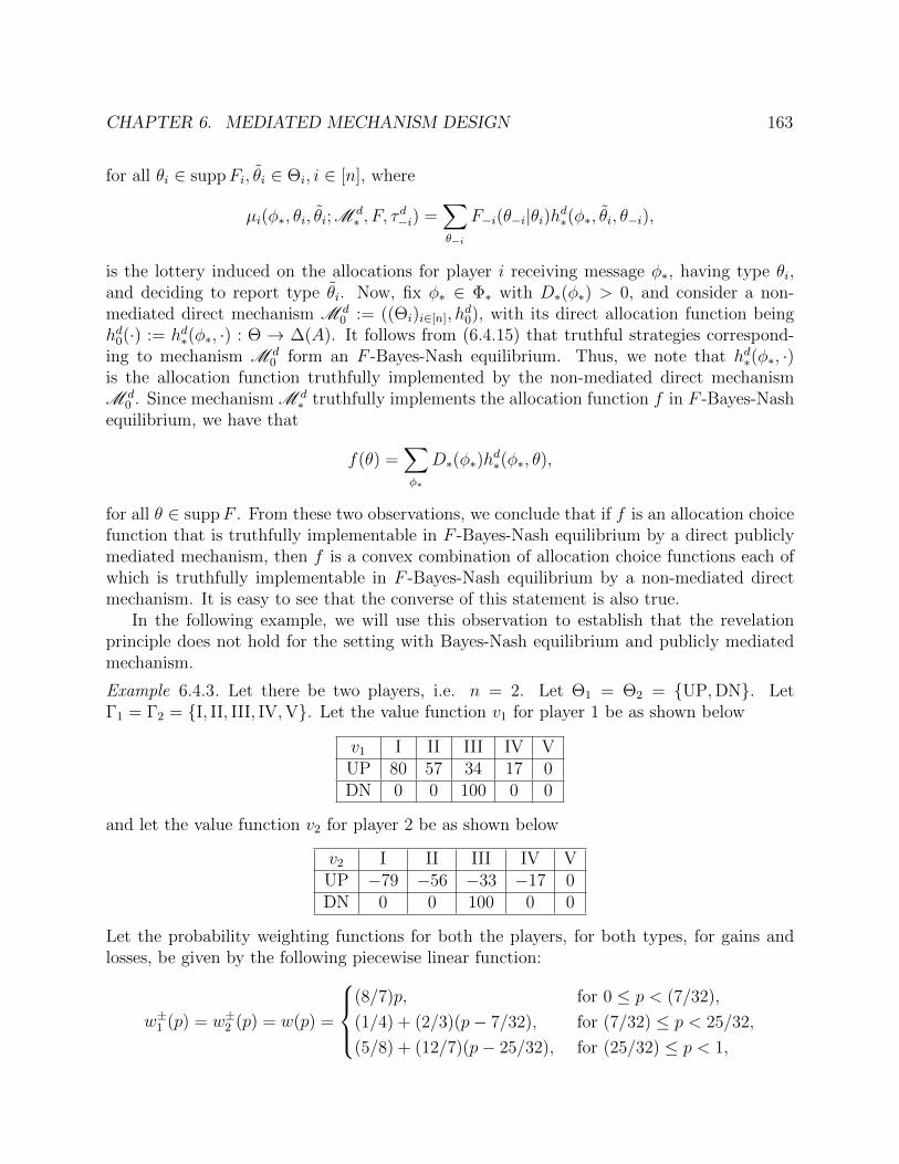
CHAPTER 6. MEDIATED MECHANISM DESIGN 163
for all θi ∈ suppFi, θi ∈ Θi, i ∈ [n], where
µi(φ∗, θi, θi; Md∗ , F, τ
d−i) =
∑θ−i
F−i(θ−i|θi)hd∗(φ∗, θi, θ−i),
is the lottery induced on the allocations for player i receiving message φ∗, having type θi,and deciding to report type θi. Now, fix φ∗ ∈ Φ∗ with D∗(φ∗) > 0, and consider a non-mediated direct mechanism M d
0 := ((Θi)i∈[n], hd0), with its direct allocation function being
hd0(·) := hd∗(φ∗, ·) : Θ → ∆(A). It follows from (6.4.15) that truthful strategies correspond-ing to mechanism M d
0 form an F -Bayes-Nash equilibrium. Thus, we note that hd∗(φ∗, ·)is the allocation function truthfully implemented by the non-mediated direct mechanismM d
0 . Since mechanism M d∗ truthfully implements the allocation function f in F -Bayes-Nash
equilibrium, we have that
f(θ) =∑φ∗
D∗(φ∗)hd∗(φ∗, θ),
for all θ ∈ suppF . From these two observations, we conclude that if f is an allocation choicefunction that is truthfully implementable in F -Bayes-Nash equilibrium by a direct publiclymediated mechanism, then f is a convex combination of allocation choice functions each ofwhich is truthfully implementable in F -Bayes-Nash equilibrium by a non-mediated directmechanism. It is easy to see that the converse of this statement is also true.
In the following example, we will use this observation to establish that the revelationprinciple does not hold for the setting with Bayes-Nash equilibrium and publicly mediatedmechanism.
Example 6.4.3. Let there be two players, i.e. n = 2. Let Θ1 = Θ2 = UP,DN. LetΓ1 = Γ2 = I, II, III, IV,V. Let the value function v1 for player 1 be as shown below
v1 I II III IV VUP 80 57 34 17 0DN 0 0 100 0 0
and let the value function v2 for player 2 be as shown below
v2 I II III IV VUP −79 −56 −33 −17 0DN 0 0 100 0 0
Let the probability weighting functions for both the players, for both types, for gains andlosses, be given by the following piecewise linear function:
w±1 (p) = w±2 (p) = w(p) =
(8/7)p, for 0 ≤ p < (7/32),
(1/4) + (2/3)(p− 7/32), for (7/32) ≤ p < 25/32,
(5/8) + (12/7)(p− 25/32), for (25/32) ≤ p < 1,

CHAPTER 6. MEDIATED MECHANISM DESIGN 164
(See the probability weighting function for gains in Figure 6.1.) Let the prior distribution Fbe such that the types of the players are independently sampled with probabilities,
P(UP) = 3/4,P(DN) = 1/4. (6.4.16)
Let A = a, b, c. Let
ζ(a) = (1/2, (I, I)); (1/2, (V,V)),ζ(b) = (1/2, (II, II)); (1/2, (IV, IV)),ζ(c) = (III, III).
Consider the allocation choice function f ∗ given by
f ∗(DN, θ2) = f ∗(θ1,DN) = c, ∀θ1 ∈ Θ1, θ2 ∈ Θ2
f ∗(UP,UP) = (1/2, a); (1/2, b).
We will now show that f ∗ is implementable in F -Bayes-Nash equilibrium by a publiclymediated mechanism. In fact, we will show that f ∗ is implementable in F -Bayes-Nashequilibrium by a non-mediated mechanism. We will then show that f ∗ cannot be a convexcombination of allocation choice functions each of which is truthfully implementable by anon-mediated direct mechanism. This will give us that f ∗ is not truthfully implementable inF -Bayes-Nash equilibrium by a direct publicly mediated mechanism. We will then concludethat the revelation principle does not hold for the setting with Bayes-Nash equilibrium andpublicly mediated mechanism.
Consider the mechanism M0 = ((Ψi)i∈[n], h0), where Ψ1 = UPa,UPb,DN, Ψ2 =UP,DN, and the allocation function h0 is given by
h0(DN, ψ2) = h0(ψ1,DN) = c, ∀ψ1 ∈ Ψ1, ψ2 ∈ Ψ2,
h0(UPa,UP) = a,
h0(UPa,UP) = b.
Consider the strategy σ1 for player 1 given by
σ1(UP) = (1/2,UPa); (1/2,UPb),σ1(DN) = DN,
and the strategy σ2 for player 2 given by
σ2(UP) = UP,
σ2(DN) = DN.
It is easy to see that this induces the allocation choice function f ∗.

CHAPTER 6. MEDIATED MECHANISM DESIGN 165
We will now verify that σ is an F -Bayes-Nash equilibrium for M0. If player 1 has typeUP, then the CPT values of the lotteries faced by her corresponding to her signals are asfollows:
WUP1 (µ1(UP,UPa; M0, F, σ−1)) = V UP
1 ((3/8, I); (0, II); (1/4, III); (0, IV); (3/8,V))= 46w(3/8) + 34w(5/8)
= 34.
WUP1 (µ1(UP,UPb; M0, F, σ−1)) = V UP
1 ((0, I); (3/8, II); (1/4, III); (3/8, IV); (0,V))= 23w(3/8) + 17w(5/8) + 17
= 34.
WUP1 (µ1(UP,DN; M0, F, σ−1)) = V UP
1 (III) = 34.
Thus player 1 is indifferent between all signals when she has type UP and so the strategy ofsignaling σ1(UP) = (1/2,UPa); (1/2,UPb) is optimal for her.
If player 1 has type DN, then III is the best outcome and she receives this lottery if shesignals DN. Thus DN dominates any other strategy, in particular, signaling UPa or UPb.
If player 2 has type UP, then the CPT values of the lotteries faced by her correspondingto her signals are as follows:
WUP2 (µ1(UP,UP; M0, F, σ−2)) = V UP
1 ((3/16, I); (3/16, II); (1/4, III); (3/16, IV); (3/16,V))= −23w(3/16)− 23w(3/8)− 16w(5/8)− 17w(13/16)
= −32.94.
WUP2 (µ1(UP,DN; M0, F, σ−2)) = V UP
1 (III) = −33.
Hence the strategy of signaling σ2(UP) = UP is optimal for player 2 when she has type UP.If player 2 has type DN, then III is the best outcome and she receives this lottery if she
signals DN. Thus DN dominates any other strategy, in particular, signaling UP.This shows that σ is an F -Bayes-Nash equilibrium for M0, and hence establishes that f ∗
is implementable in F -Bayes-Nash equilibrium by a non-mediated mechanism.Suppose f ∗ were a convex combination of allocation choice functions each of which is
truthfully implementable by a non-mediated direct mechanism. Let f be one of the allocationchoice functions in this convex combination. Since f ∗(DN, θ2) = f ∗(θ1,DN) = c for all θ1, θ2,and since c is an extreme point of the simplex ∆(A), we get that
f(DN, θ2) = f(θ1,DN) = c, ∀θ1 ∈ Θ1, θ2 ∈ Θ2. (6.4.17)
Similarly, since f ∗(UP,UP) lies on the line joining the vertices a and b of the simplex∆(A), we get that
f(UP,UP) = (x, a); (1− x, b), (6.4.18)

CHAPTER 6. MEDIATED MECHANISM DESIGN 166
0 0.58 1
34
33.38
x
E3(x
)
Figure 6.1: Plot of expression E3(x) in Example 6.4.3.
where 0 ≤ x ≤ 1.Let f be truthfully implementable in F -Bayes-Nash equilibrium by the non-mediated
direct mechanism M d0 = hd0. Then hd0 = f . If player 1 has type UP, then the lottery faced
by her if she reports UP is given by
L1(µ1(UP,UP; M d0 , F, σ
d−1)) = (3x/8, I); (3(1−x)/8, II); (1/4, III); (3(1−x)/8, IV); (3x/8,V),
where σd−1 = σd2 is the truthful strategy of player 2. Let
E3(x) := 23w
(3x
8
)+ 23w
(3
8
)+ 17w
(5
8
)+ 17w
(1− 3x
8
),
for x ∈ [0, 1]. We observe that E3(x) is maximum at x = 0 and x = 1, and for all x ∈ (0, 1),E3(x) < 34. (See Figure 6.1.)
Now, unless x = 0 or x = 1, player 1 will defect from the truthful strategy and reportDN when her true type is UP, because if she does so the allocation c will be implemented bythe system operator, which results in her outcome III, hence giving her a value of 34. Thus,x = 0 or x = 1.
If player 2 has type UP, then the lottery faced by her if she reports UP is given by
L2(µ2(UP,UP; M d0 , F, σ
d−2)) = (3x/8, I); (3(1−x)/8, II); (1/4, III); (3(1−x)/8, IV); (3x/8,V),
where σd−2 = σd1 is the truthful strategy of player 1. If x = 0, then the CPT value for player2 is given by
V UP2 ((0, I); (3/8, II); (1/4, III); (3/8, IV); (0,V)
= −23w(3/8)− 16w(5/8)− 17
= −33.48.

CHAPTER 6. MEDIATED MECHANISM DESIGN 167
If x = 1, then the CPT value for player 2 is given by
V UP2 ((3/8, I); (0, II); (1/4, III); (0, IV); (3/8,V)
= −46w(3/8)− 33w(5/8)
= −33.48.
Now, if x = 0 or x = 1, player 2 will defect from the truthful strategy and report DN whenher true type is UP, because if she does so the allocation c will be implemented by thesystem operator, which results in her outcome III, hence giving her a value of −33. Thusx cannot be 0 or 1, leading to a contradiction. Thus, f ∗ cannot be a convex combinationof allocation choice functions each of which is truthfully implementable by a non-mediateddirect mechanism. This completes the argument.
Example 6.4.4. We will now show that in the setting with dominant equilibrium and mediatedmechanism, the revelation principle does not hold. This happens even when the players haveEUT preferences. Let there be two players, i.e. n = 2. Let Θ1 = UP,DN, Θ2 = UN.Let Γ1 = Γ2 = A = I, II, III. Let the value functions v1 and v2 be given by
v1 I II IIIUP 5 −10 10DN 0 0 10
v2 I II IIIUN 5 −10 −5
Both the players have EUT preferences (i.e, their probability weighting functions are identityfunctions).
Consider the allocation choice function f given by
f(UP,UN) = I and f(DN,UN) = III.
We claim that this allocation choice function cannot be implemented by any direct mediatedmechanism in truthful dominant equilibrium. To see this, suppose there exists a directmediated mechanism M d = ((Φ1,Φ2), D, h) that truthfully implements the allocation choicefunction f in dominant equilibrium. Consider the lottery
µ1(φ1, θ1, θ′1; M d,UN) =
∑φ2
D−1(φ2|φ1)h(φ, θ′1,UN),
for player 1 when she receives message φ1, has type θ1, chooses to report θ′1 (and triviallybelieves that player 2 reports type UN since that is the only type for player 2). Note thatµ1(φ1, θ1, θ
′1; M d,UN) does not depend on the type θ1 of player 1. For any message φ1,
consider the function π1(φ1, ·) : Θ→ ∆(A) given by
π1(φ1, θ1,UN) := µ1(φ1, θ1, θ1; M d,UN).
Note that π1(φ1, ·) is an allocation choice function. Since M d truthfully implements f , wehave
f(θ1,UN) =∑φ1
D1(φ1)πi(φ1, θ1,UN),

CHAPTER 6. MEDIATED MECHANISM DESIGN 168
for θ1 = UP and DN. Thus, the allocation choice function f is a convex combination of thefunctions π1(φ1, ·)φ1 . Since f is an extreme point of the convex set of all allocation choicefunctions, we get that π1(φ1, ·) = f(·) for all φ1. Since truthful strategies are assumed toform a dominant equilibrium, we should have
W θ11 (µ1(φ1, θ1, θ1; M ,UN)) ≥ W θ1
1 (µ1(φ1, θ1, θ′1; M ,UN)),
for θ1 = UP and DN. However,
WUP1 (µ1(φ1,UP,UP; M ,UN)) = WUP
1 (π1(φ1,UP,UN))
= WUP1 (f(UP,UN))
= WUP1 (I) = 5 < 10 = WUP
1 (III)
= WUP1 (f(DN,UN))
= WUP1 (π1(φ1,DN,UN))
= WUP1 (µ1(φ1,UP,DN; M ,UN)).
This is a contradiction, and hence, we conclude that the allocation choice function f is nottruthfully implementable by a direct mediated mechanism in dominant equilibrium.
We will now show that the allocation choice function f can be implemented by mediatedmechanism in dominant equilibrium if we use the message sets Φ1 = C,Φ2 = L,R andthe signal sets Ψ1 = UP,DN,Ψ2 = L,R. Let the mediator distribution be given byD(C,L) = D(C,R) = 1/2. Let the mediated allocation function h : Φ×Ψ→ ∆(A) be givenby
h(C,L,UP, L) = I,
h(C,L,UP, R) = I,
h(C,L,DN, L) = III,
h(C,L,DN, R) = II,
h(C,R,UP, L) = I,
h(C,R,UP, R) = I,
h(C,R,DN, L) = II,
h(C,R,DN, R) = III.
Let M = ((C, (L,R)), D, h) be the mediated mechanism. Now, consider the strategiesσ1 : Φ1 ×Θ1 → ∆(Ψ1) and σ2 : Φ2 ×Θ2 → ∆(Ψ2) given by
σ1(C,UP) = UP and σ1(C,DN) = DN,
σ2(L,UN) = L and σ1(R,UN) = R.

CHAPTER 6. MEDIATED MECHANISM DESIGN 169
We will now verify that these strategies form a dominant equilibrium and implement theallocation choice function f . Let us first verify that σ1 is a dominant strategy. We have,
WUP1 (µ1(C,UP,UP; M , L)) = 0.5vUP
1 (h(C,L,UP, L)) + 0.5vUP1 (h(C,R,UP, L)) = 5,
WUP1 (µ1(C,UP,DN; M , L)) = 0.5vUP
1 (h(C,L,DN, L)) + 0.5vUP1 (h(C,R,DN, L)) = 0,
WUP1 (µ1(C,UP,UP; M , R)) = 0.5vUP
1 (h(C,L,UP, R)) + 0.5vUP1 (h(C,R,UP, R)) = 5,
WUP1 (µ1(C,UP,DN; M , R)) = 0.5vUP
1 (h(C,L,DN, R)) + 0.5vUP1 (h(C,R,DN, R)) = 0.
Thus, when player 1 has type UP, it is in her best interest to report UP in both the casescorresponding to her belief about the report by player 2, namely, L and R. On the otherhand, when player 1 has type DN, we have
WDN1 (µ1(C,DN,UP; M , L)) = 0.5vDN
1 (h(C,L,UP, L)) + 0.5vDN1 (h(C,R,UP, L)) = 0,
WDN1 (µ1(C,DN,DN; M , L)) = 0.5vDN
1 (h(C,L,DN, L)) + 0.5vDN1 (h(C,R,DN, L)) = 5,
WDN1 (µ1(C,DN,UP; M , R)) = 0.5vDN
1 (h(C,L,UP, R)) + 0.5vDN1 (h(C,R,UP, R)) = 0,
WDN1 (µ1(C,DN,DN; M , R)) = 0.5vDN
1 (h(C,L,DN, R)) + 0.5vDN1 (h(C,R,DN, R)) = 5.
Thus, when player 1 has type DN, it is in her best interest to report DN in both the casescorresponding to her belief about the report by player 2, namely, L and R. Hence, σ1 is adominant strategy for player 1. For player 2, we have
WUN2 (µ2(L,UN, L; M ,UP)) = vUN
2 (h(C,L,UP, L)) = 5,
WUN2 (µ2(L,UN, R; M ,UP)) = vUN
2 (h(C,L,UP, R)) = 5,
WUN2 (µ2(L,UN, L; M ,DN)) = vUN
2 (h(C,L,DN, L)) = −5,
WUN2 (µ2(L,UN, R; M ,DN)) = vUN
2 (h(C,L,DN, R)) = −10.
Hence, σ2 is a dominant strategy for player 1.Thus, σ is a dominant equilibrium. It is easy to verify that it implements the allocation
choice function f for the mechanism M . We thus conclude that the revelation principle doesnot hold in the setting with dominant equilibrium and mediated mechanism.
6.5 Summary
In this chapter, we considered mechanism design for CPT players and in this process wediscovered several important concepts that have gone unnoticed in the classical setting withEUT players. Namely, we saw that it is important to treat the allocation set and the outcomeset of each player separately, both from theoretical as well as behavioral point of view. Wealso saw that we need to be careful while considering the notion of dominant strategieswith CPT players and we need to treat the two notions of dominant equilibrium and belief-dominant equilibrium separately. Next, we saw that the generalized framework of mediatedmechanisms recovers the coveted revelation principle.

CHAPTER 6. MEDIATED MECHANISM DESIGN 170
Notice that in Table 6.1, we have a tick mark in each row. This tells us that anythingthat can be implemented by a non-mediated mechanism (possibly with general signals) canbe truthfully implemented by a direct (publicly or general) mediated mechanism. Indeed,if a social choice function is implementable in Bayes-Nash equilibrium by a non-mediatedequilibrium, then it is truthfully implementable in Bayes-Nash equilibrium by a direct me-diated mechanism. Further, the setting for implementability in Bayes-Nash equilibrium bymediated mechanisms is favorable in the sense that the revelation principle holds here andwe can restrict our attention to truthful implementability by direct mediated mechanisms.In the setting for implementability in dominant equilibrium, if a social choice function isimplementable in dominant equilibrium by a non-mediated equilibrium, then it is truthfullyimplementable in dominant equilibrium by a direct publicly mediated mechanism. And,the setting for implementability in dominant equilibrium by publicly mediated mechanismsis favorable in the sense that the revelation principle holds here and we can restrict ourattention to truthful implementability by direct publicly mediated mechanisms. Finally,in the setting of implementability in belief-dominant equilibrium, if a social choice func-tion is implementable in belief-dominant equilibrium by a non-mediated equilibrium, thenit is truthfully implementable in belief-dominant equilibrium by a direct publicly mediatedmechanism. Besides, the revelation principle holds for both publicly mediated and mediatedmechanisms in the setting of belief-dominant equilibrium.
It is worthwhile to repeat the importance of truthful implementability of social choicefunctions by direct (mediated) mechanisms, namely, we can restrict our attention to truthfulstrategies. We will now see some of the benefits of the revelation principle and truthfulstrategies that make applications of mechanism design practical for large-scale implementa-tion with participants who can be both, humans and machines.
Generally in the settings where agents exhibit deviations from expected utility behavior,one would expect that the participating agents do not possess large computational power.Hence, truthful strategies are especially suitable for such settings in contrast to the morecomplicated strategies that are permitted by the concept of Bayes-Nash equilibrium. Onthe other hand, if our participating agents do not possess large computational power, thenit is natural to question if they have the ability to exhibit strategic behavior, in particularthe requirement that the strategies form a Bayes-Nash equilibrium (or dominant equilibriumor belief-dominant equilibrium). However, there can also be agents in the system who dopossess large computational power. Indeed, most of the systems such as online auctionsand marketplaces or networked-systems such as transportation networks, Internet routingnetworks, etc. are comprised of players having varying degrees of computational and strategicabilities. For example, a firm participating in an online marketplace has the resources toestimate the common prior and other players’ strategies through extensive data collection,and thus can develop optimal strategies. On the other hand, individual agents participatingin the same system often lack such resources. When truthful strategies are in equilibrium,we get the best of both the worlds – it is easy for the players with limited resources toimplement optimal strategies and at the same time there is no incentive for the players withlarge resources to deviate from these strategies.
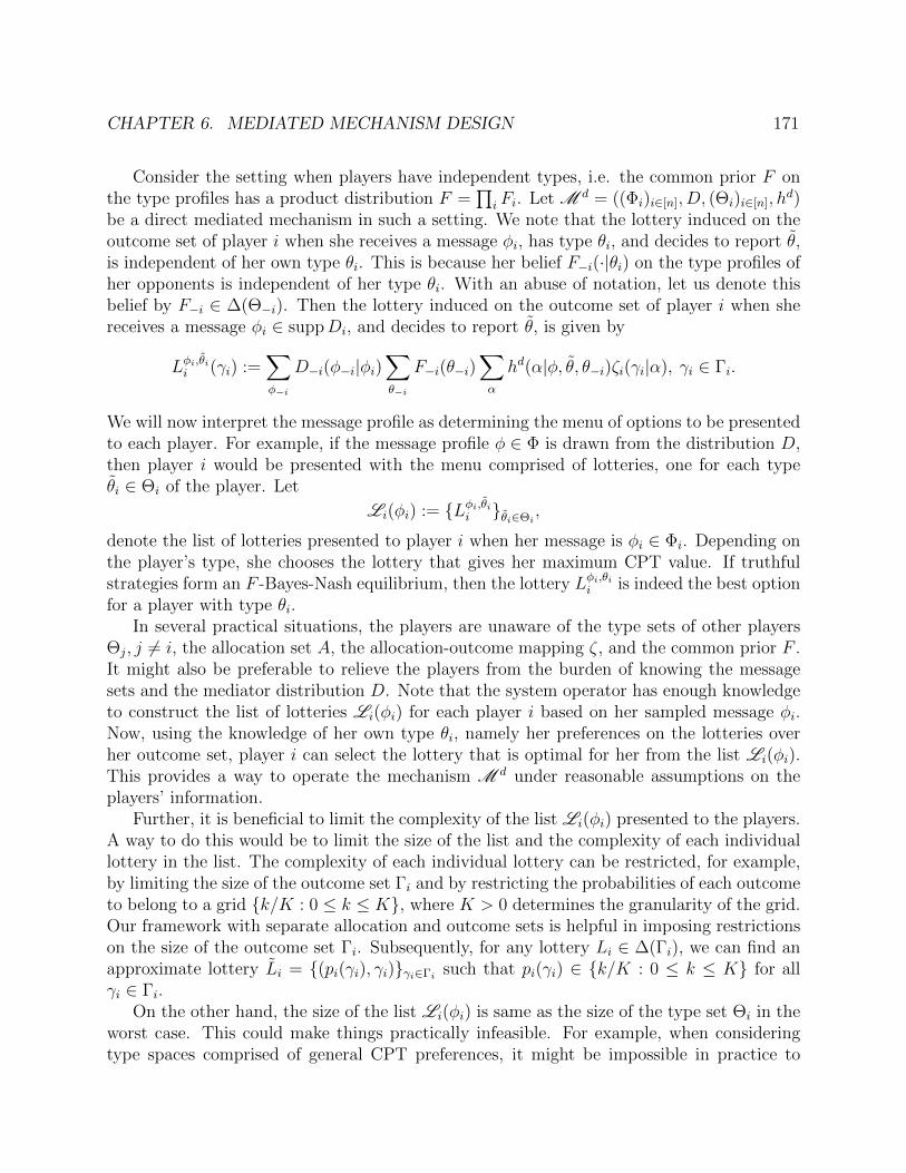
CHAPTER 6. MEDIATED MECHANISM DESIGN 171
Consider the setting when players have independent types, i.e. the common prior F onthe type profiles has a product distribution F =
∏i Fi. Let M d = ((Φi)i∈[n], D, (Θi)i∈[n], h
d)be a direct mediated mechanism in such a setting. We note that the lottery induced on theoutcome set of player i when she receives a message φi, has type θi, and decides to report θ,is independent of her own type θi. This is because her belief F−i(·|θi) on the type profiles ofher opponents is independent of her type θi. With an abuse of notation, let us denote thisbelief by F−i ∈ ∆(Θ−i). Then the lottery induced on the outcome set of player i when shereceives a message φi ∈ suppDi, and decides to report θ, is given by
Lφi,θii (γi) :=∑φ−i
D−i(φ−i|φi)∑θ−i
F−i(θ−i)∑α
hd(α|φ, θ, θ−i)ζi(γi|α), γi ∈ Γi.
We will now interpret the message profile as determining the menu of options to be presentedto each player. For example, if the message profile φ ∈ Φ is drawn from the distribution D,then player i would be presented with the menu comprised of lotteries, one for each typeθi ∈ Θi of the player. Let
Li(φi) := Lφi,θii θi∈Θi,
denote the list of lotteries presented to player i when her message is φi ∈ Φi. Depending onthe player’s type, she chooses the lottery that gives her maximum CPT value. If truthfulstrategies form an F -Bayes-Nash equilibrium, then the lottery Lφi,θii is indeed the best optionfor a player with type θi.
In several practical situations, the players are unaware of the type sets of other playersΘj, j 6= i, the allocation set A, the allocation-outcome mapping ζ, and the common prior F .It might also be preferable to relieve the players from the burden of knowing the messagesets and the mediator distribution D. Note that the system operator has enough knowledgeto construct the list of lotteries Li(φi) for each player i based on her sampled message φi.Now, using the knowledge of her own type θi, namely her preferences on the lotteries overher outcome set, player i can select the lottery that is optimal for her from the list Li(φi).This provides a way to operate the mechanism M d under reasonable assumptions on theplayers’ information.
Further, it is beneficial to limit the complexity of the list Li(φi) presented to the players.A way to do this would be to limit the size of the list and the complexity of each individuallottery in the list. The complexity of each individual lottery can be restricted, for example,by limiting the size of the outcome set Γi and by restricting the probabilities of each outcometo belong to a grid k/K : 0 ≤ k ≤ K, where K > 0 determines the granularity of the grid.Our framework with separate allocation and outcome sets is helpful in imposing restrictionson the size of the outcome set Γi. Subsequently, for any lottery Li ∈ ∆(Γi), we can find anapproximate lottery Li = (pi(γi), γi)γi∈Γi such that pi(γi) ∈ k/K : 0 ≤ k ≤ K for allγi ∈ Γi.
On the other hand, the size of the list Li(φi) is same as the size of the type set Θi in theworst case. This could make things practically infeasible. For example, when consideringtype spaces comprised of general CPT preferences, it might be impossible in practice to
CHAPTER 6. MEDIATED MECHANISM DESIGN 172
elicit the probability weighting functions from the agents. Restricting the type space canlead to inefficient social choice functions. The mediated mechanism design framework couldallow us to limit the size of menu options and at the same time have diversity in the socialchoice function across different types of the players, facilitated by the messaging stage. Suchmultiple communication rounds have been studied under EUT and there is an extensive lit-erature concerning the communication requirements in mechanism design. (See [86] and thereferences therein. See also the literature on computational mechanism design [36].) Giventhat the non-EUT preferences can reliably be applied only to non-dynamic decision-making,we are especially interested in mechanisms that have a single stage of mediator messages towhich the participating agents respond optimally by choosing their best option. It would beinteresting to study the design of mechanisms that optimally elicit CPT preferences undercommunication restrictions such as limiting the size of the menu options. For example, wecould consider mechanism designs where the mediated allocation function hd for a directmediated mechanism has to satisfy |Li(φi| ≤ B, for all messages φi, for some bound B.
In this chapter, we focused on the mechanism design framework and the revelation prin-ciple for agents having CPT preferences. It is just the first step towards mechanism designfor non-EUT players, with several interesting directions for future work. In the next chapter,we will discuss some of these directions.
Appendix
6.A Proof of the Revelation Principle
We will first consider the revelation principle in the setting of mediated mechanisms. Thiscorresponds to statement (i) and a part of statement (ii) of Theorem 6.4.1. In this settingwe will show that if an allocation choice function f is implementable in Bayes-Nash equi-librium (resp. belief-dominant equilibrium) by a mediated mechanism then it is truthfullyimplementable in Bayes-Nash equilibrium (resp. belief-dominant equilibrium) by a directmediated mechanism. We will then consider the setting of publicly mediated mechanismsand show that if an allocation choice function f is implementable in dominant equilibrium(resp. belief-dominant equilibrium) by a publicly mediated mechanism then it is truthfullyimplementable in dominant equilibrium (resp. belief-dominant equilibrium) by a direct pub-licly mediated mechanism. This will complete the proof of statement (ii) and the remainingpart of statement (iii) of Theorem 6.4.1.
For the first setting, let
M = ((Φi)i∈[n], D, (Ψi)i∈[n], h),
be a mediated mechanism and let τ be a strategy profile that induces f for this mechanism.Consider now the direct mediated mechanism
M d = ((Φ′i)i∈[n], D′, (Θi)i∈[n], h
d),

CHAPTER 6. MEDIATED MECHANISM DESIGN 173
where the message set is given by
Φ′i := Φi × (Ψi)Θi , (6.A.1)
with a typical element denoted by
φ′i := (φi, (ψθ′ii )θ′i∈Θi), (6.A.2)
and the mediator distribution D′ is given by
D′(φ′) := D(φ)∏i∈[n]
∏θ′i∈Θi
τi
(ψθ′ii |φi, θ′i
)for all φ′ ∈ Φ′. (6.A.3)
The modified mediator messages and the mediator distribution can be interpreted as encap-sulating the randomness in the strategies of the players for each of their types into theirprivate messages.
We now observe that
D′i(φ′i) = Di(φi)
∏θ′i∈Θi
τi
(ψθ′ii |φi, θ′i
), (6.A.4)
and ∑φ′i∈Φ′i
D′i(φ′i) =
∑φ′∈Φ′
D′(φ′) = 1.
Thus, D′ ∈ ∆(Φ′) is indeed a valid distribution. Equation (6.A.4) can be formally proved asfollows:
D′i(φ′i) =
∑φ′−i∈Φ′−i
D′(φ′i, φ′−i)
=∑
φ−i∈Φ−i
D(φi, φ−i)∑
(ψθ′jj )θ′
j∈Θj ,j 6=i
∈∏j 6=i(Ψj)
Θj
∏j 6=i
∏θ′j∈Θj
τj
(ψθ′jj |φj, θ′j
) ∏θ′i∈Θi
τi
(ψθ′ii |φi, θ′i
)
=∑
φ−i∈Φ−i
D(φi, φ−i)∏θ′i∈Θi
τi
(ψθ′ii |φi, θ′i
)∏j 6=i
∏θ′j∈Θj
∑ψθ′jj ∈Ψj
τj
(ψθ′jj |φj, θ′j
)=
∑φ−i∈Φ−i
D(φi, φ−i)∏θ′i∈Θi
τi
(ψθ′ii |φi, θ′i
)∏j 6=i
∏θ′j∈Θj
1

CHAPTER 6. MEDIATED MECHANISM DESIGN 174
= Di(φi)∏θ′i∈Θi
τi
(ψθ′ii |φi, θ′i
).
Let the direct mediated allocation function be given by
hd(φ′, θ′) := h
(φ,(ψθ′ii
)i∈[n]
)for all φ′ ∈ Φ′, θ′ ∈ Θ. (6.A.5)
Note that the construction of the direct mediated mechanism is independent of the priordistribution F .
The modified mediator messages and the direct mediated allocation function hd essen-tially transfer the randomness in the strategies of the players to the mediator messages, thusallowing each player to simply report her type. We observe that the truthful strategies
τ di (θi|φ′i, θi) = 1θi = θi,for all players i, implement the allocation choice function f for the direct mediated mechanismM d. Here is a formal proof.
Let us compute the distribution on the allocation set induced by the truthful strategyfor the direct mediated mechanism. For any fixed θ ∈ Θ and α ∈ A, we have∑
φ′∈Φ′
D′(φ′)∑θ∈Θ
∏i∈[n]
τ di (θi|φ′i, θi)
hd(α|φ′, θ)
=∑φ′∈Φ′
D′(φ′)∑θ∈Θ
∏i∈[n]
1θi = θi
hd(α|φ′, θ)
... because τ d is a truthful strategy
=∑φ′∈Φ′
D′(φ′)hd(α|φ′, θ)
=∑φ′∈Φ′
D(φ)
∏i∈[n]
∏θ′i∈Θi
τi
(ψθ′ii |φi, θ′i
)hd(α|φ′, θ)
... from (6.A.3)
=∑φ∈Φ
D(φ)∑
(ψθ′ii )θ′
i∈Θi,i∈[n]
∈∏i∈[n](Ψi)
Θi
∏i∈[n]
∏θ′i∈Θi
τi
(ψθ′ii |φi, θ′i
)hd(α|φ′, θ)
... from (6.A.2)
=∑φ∈Φ
D(φ)∑
(ψθ′ii )θ′
i∈Θi,i∈[n]
∈∏i∈[n](Ψi)
Θi
∏i∈[n]
∏θ′i∈Θi
τi
(ψθ′ii |φi, θ′i
)h(α∣∣φ, (ψθii )i∈[n]
)

CHAPTER 6. MEDIATED MECHANISM DESIGN 175
... from (6.A.5)
=∑φ∈Φ
D(φ)∑
(ψθii )i∈[n]
∈∏i∈[n] Ψi
∑(ψθ′ii )θ′
i6=θi,i∈[n]
∈∏i∈[n](Ψi)
Θi\θi
∏i∈[n]
∏θ′i 6=θi
τi
(ψθ′ii |φi, θ′i
)
×
∏i∈[n]
τi(ψθii |φi, θi
)h(α∣∣φ, (ψθii )i∈[n]
)
=∑φ∈Φ
D(φ)∑
(ψθii )i∈[n]
∈∏i∈[n] Ψi
∏i∈[n]
τi(ψθii |φi, θi
)h(α∣∣φ, (ψθii )i∈[n]
)
×∑
(ψθ′ii )θ′
i6=θi,i∈[n]
∈∏i∈[n](Ψi)
Θi\θi
∏i∈[n]
∏θ′i 6=θi
τi
(ψθ′ii |φi, θ′i
)
=∑φ∈Φ
D(φ)∑
(ψθii )i∈[n]
∈∏i∈[n] Ψi
∏i∈[n]
τi(ψθii |φi, θi
)h(α∣∣φ, (ψθii )i∈[n]
)
×
∏i∈[n]
∏θ′i 6=θi
∑ψθ′ii ∈Ψi
τi
(ψθ′ii |φi, θ′i
)=∑φ∈Φ
D(φ)∑
(ψθii )i∈[n]
∈∏i∈[n] Ψi
∏i∈[n]
τi(ψθii |φi, θi
)h(α∣∣φ, (ψθii )i∈[n]
)∏i∈[n]
∏θ′i 6=θi
1
... because τi(·|φi, θ′i) ∈ ∆(Ψi)
=∑φ∈Φ
D(φ)∑ψ∈Ψ
∏i∈[n]
τi (ψi|φi, θi)
h(α∣∣φ, ψ)
= f(α|θ) if θ ∈ suppF
... from (6.4.8).
This confirms that the truthful strategy profile implements the social choice function for thedirect mediated mechanism M d.
We will now show that if τ is an F -Bayes-Nash equilibrium for M , then τ d is an F -Bayes-Nash equilibrium for M d. We will then show that if τ is a belief-dominant equilibrium

CHAPTER 6. MEDIATED MECHANISM DESIGN 176
for M , then τ d is a belief-dominant equilibrium for M d. To prove these two statements,we first make the following observation concerning the lottery induced over the allocationsfor player i in the setting of the direct mediated mechanism M d, when she receives the
message φ′i := (φi, (ψθ′ii )θ′i∈Θi) ∈ suppD′i, has type θi ∈ Θi, has a belief G′−i ∈ ∆(Θ−i) on
the opponents’ type reports (which are the signals of the opponents in this direct mediatedmechanism), and decides to report θi. The lottery induced over the allocations for player isatisfies
µ′i(φ′i, θi, θi; M
d, G′−i) :=∑
φ′−i∈Φ′−i
D′−i(φ′−i|φ′i)
∑θ−i∈Θ−i
G′−i(θ−i)hd(φ′, θi, θ−i)
=∑
φ−i∈Φ−i
D−i(φ−i|φi)∑
θ−i∈Θ−i
G′−i(θ−i)
×∑ψ−i
(∏j 6=i
τj (ψj|φj, θj)
)h(φ, ψθii , ψ−i
). (6.A.6)
We give a formal proof of this in Appendix 6.B. Let us see how this observation helps us provethe two statements above, namely, τ d is an equilibrium (F -Bayes-Nash or belief-dominantresp.) of M d given that τ is an equilibrium (F -Bayes-Nash or belief-dominant resp.) of M .
Suppose F is the common prior and τ is an F -Bayes-Nash equilibrium for the mediatedmechanism M . Let φ′i ∈ suppD′i and θi ∈ suppFi. From (6.A.4), we know that D′i(φ
′i) > 0
implies Di(φi) > 0 and τi(ψθ′ii |φi, θ′i) > 0, for all θ′i ∈ Θi, (and in particular, we have
τi(ψθii |φi, θi) > 0). Since τ is a Bayes-Nash equilibrium for M , we have
W θii
(µi(φi, θi, ψ
θii ; M , F, τ−i)
)≥ W θi
i
(µi(φi, θi, ψi; M , F, τ−i)
),
for all ψi ∈ Ψi. (Note that ψθii ∈ supp τi(·|φi, θi), φi ∈ suppDi, θi ∈ suppFi.) TakingG′−i = F−i(·|θi) in (6.A.6), we get that
µ′i(φ′i, θi, θi; M
d, F, τ d−i) = µi(φi, θi, ψθii ; M , F, τ−i), (6.A.7)
for all θi ∈ Θi, and thus,
W θii
(µ′i(φ
′i, θi, θi; M
d, F, τ d−i))
= W θii
(µi(φi, θi, ψ
θii ; M , F, τ−i)
)≥ W θi
i
(µi(φi, θi, ψ
θii ; M , F, τ−i)
)= W θi
i
(µ′i(φ
′i, θi, θi; M
d, F, τ d−i)), (6.A.8)
for all θi ∈ Θi. This establishes that the truthful strategy τ d is an F -Bayes-Nash equilibriumfor M .

CHAPTER 6. MEDIATED MECHANISM DESIGN 177
Now suppose τ is a belief-dominant strategy for M . Let φ′i ∈ suppD′i and θi ∈ Θi. Again,this implies Di(φi) > 0 and ψθii ∈ supp τi(φi, θi). Corresponding to a belief G′−i ∈ ∆(Θ−i),consider the belief G−i ∈ ∆(Ψ−i) given by
G−i(ψ−i) :=∑
φ−i∈Φ−i
D−i(φ−i|φi)∑
θ−i∈Θ−i
G′−i(θ−i)
(∏j 6=i
τj (ψj|φj, θj)
)(6.A.9)
Then, from (6.A.6), we have that
µ′i(φ′i, θi, θi; M
d, G′−i) = µi(φi, θi, ψθii ; M , G−i) (6.A.10)
Noting that ψθii ∈ supp τi(φi, θi) for all θi ∈ Θi and φi ∈ suppDi, and τi being a belief-dominant strategy, we get that
W θii
(µ′i(φ
′i, θi, θi; M
d, G′−i))≥ W θi
i
(µ′i(φ
′i, θi, θi; M
d, G′−i))
(6.A.11)
for all θi ∈ Θi. Thus, the truthful strategy τ d is a belief-dominant strategy for M d.This completes the proof of statement (i) in Theorem 6.4.1 and part of statement (iii)
corresponding to mediated mechanisms. We now consider the setting of publicly mediatedmechanisms and establish the rest of the theorem.
LetM∗ = (Φ∗, D∗, (Ψi)i∈[n], h∗)
be a publicly mediated mechanism and for each player i let τi : Φ∗ × Θi → ∆(Ψi) be herstrategy such that the strategy profile τ induces the allocation choice function f for thismechanism. We now consider the direct publicly mediated mechanism
M d∗ := (Φ′∗, D
′∗, (Θi)i∈[n], h
d∗),
where the message set is given by
Φ′∗ := Φ∗ ×n∏i=1
(Ψi)Θi ,
with a typical element denoted by
φ′∗ := (φ∗, (ψθ′ii )θ′i∈Θi,i∈[n]), (6.A.12)
and the mediator distribution D′∗ is given by
D′∗(φ′∗) := D∗(φ∗)
∏i∈[n]
∏θ′i∈Θi
τi
(ψθ′ii |φi, θ′i
)for all φ′ ∈ Φ′. (6.A.13)

CHAPTER 6. MEDIATED MECHANISM DESIGN 178
Similar to the previous setting, here the modified mediator messages and the mediator dis-tribution can be interpreted as encapsulating the randomness in the strategies of the playersfor each of their types into the public messages. We can similarly verify that D′∗ is indeeda probability distribution on Φ′∗. The direct mediated allocation function hd∗ in the directpublicly mediated mechanism M d is given by
hd∗(φ′∗, θ′) := h∗
(φ∗,(ψθ′ii
)i∈[n]
)for all φ′∗ ∈ Φ′∗, θ
′ ∈ Θ. (6.A.14)
We can similarly verify that the truthful strategies
τ d(φ′∗, θi) = θi
implement the allocation choice function f for M d∗ .
Fix φ′∗ ∈ suppD′∗. Note that
hd∗(φ′∗, θi, θ−i) = h∗(φ∗, ψ
θii , (ψ
θjj )j 6=i), (6.A.15)
for all θi ∈ Θi. From (6.A.13), we have φ∗ ∈ suppD∗ and ψθii ∈ supp τi(φ∗, θi) for all θi ∈ Θi.Now suppose τ is a dominant equilibrium for M∗. The lottery induced over the allocations
for player i when she receives a publicly mediated message φ′∗, has type θi, believes that theopponents are reporting θ−i, and decides to report θi is given by
µ′i(φ′∗, θi, θi; M
d∗ , θ−i) = hd∗(φ
′∗, θi, θ−i). (6.A.16)
We get this from (6.4.9) by considering the special case of publicly mediated mechanisms.From (6.A.15), we get that this is equal to the lottery induced over the allocations for playeri when she receives a publicly mediated message φ∗, has type θi, believes that the opponentsare reporting ψ
θjj , j 6= i, and decides to report ψθi , namely,
µi(φ∗, θi, ψθi ; M∗, (ψ
θjj )j 6=i) = h∗(φ∗, ψ
θi , (ψ
θjj )j 6=i).
Since τi is a dominant strategy, φ∗ ∈ suppD∗, and ψθii ∈ supp τi(φ∗, θi), we have
W θii (µi(φ∗, θi, ψ
θii ; M∗, (ψ
θjj )j 6=i)) ≥ W θi
i (µi(φ∗, θi, ψi; M∗, (ψθjj )j 6=i)),
for all ψi ∈ Ψi. Hence, we have
W θii (µ′i(φ
′∗, θi, θi; M
d∗ , θ−i)) ≥ W θi
i (µ′i(φ′∗, θi, θi; M
d∗ , θ−i)),
for all θi ∈ Θi. Thus, τ d is a dominant equilibrium of M d∗ .
Now suppose that τ is a belief-dominant equilibrium for M∗. Consider the fixed message
φ′∗ = (φ∗, (ψθ′ii )θ′i∈Θi,i∈[n]) ∈ suppD′∗,

CHAPTER 6. MEDIATED MECHANISM DESIGN 179
as before. Corresponding to a belief G′−i ∈ ∆(Θ−i), consider G−i,∗ ∈ ∆(Ψ−i) given by
G−i,∗(ψ−i) :=∑
θ−i∈Θ−i
s.t.ψθjj =ψ−i,∀j 6=i
G′−i(θ−i), (6.A.17)
for all ψ−i ∈ Ψ−i, where ψθjj are the signals corresponding to the types as defined by the
message φ′∗.As observed in equation (6.A.16), the lottery induced over the allocations for player i,
when she receives message φ′∗, has type θi, believes that the opponents’ are reporting θ−i,and decides to report θi is given by hd∗(φ
′∗, θi, θ−i). Now suppose that she has belief G′−i on
her opponents’ type report instead. Then, the induced lottery over the allocations for playeri is given by
µ′i(φ′∗, θi, θi; M
d∗ , G
′−i) =
∑θ−i∈Θ−i
G′−i(θ−i)hd∗(φ′∗, θi, θ−i)
=∑
θ−i∈Θ−i
G′−i(θ−i)h∗(φ∗, ψθii , (ψ
θjj )j 6=i)
... from (6.A.15)
=∑
ψ−i∈Ψ−i
h∗(φ∗, ψθii , ψ−i)
∑θ−i∈Θ−i
s.t.ψθjj =ψ−i,∀j 6=i
G′−i(θ−i)
=∑
ψ−i∈Ψ−i
h∗(φ∗, ψθii , ψ−i)G−i,∗(ψ−i)
... from (6.A.17)
= µi(φ∗, θi, ψθii ; M∗, G−i,∗).
Since τ is a belief-dominant equilibrium, φ∗ ∈ suppD∗, and ψθii ∈ supp τi(φ∗, θi) for allθi ∈ Θi, we have
W θii (µi(φ∗, θi, ψ
θii ; M∗, G−i,∗) ≥ W θi
i (µi(φ∗, θi, ψi; M∗, G−i,∗),
for all ψi ∈ Ψi. Hence, we have
W θii (µ′i(φ
′∗, θi, θi; M
d∗ , G
′−i)) ≥ W θi
i (µ′i(φ′∗, θi, θi; M
d∗ , G
′−i)),
for all θi ∈ Θi. Thus, τ d is a belief-dominant equilibrium of M d∗ .
This completes the proof of the theorem.

CHAPTER 6. MEDIATED MECHANISM DESIGN 180
6.B Proof of Equation (6.A.6)
Let us recall the first setting considered in Appendix 6.A. We have a mediated mechanism
M = ((Φi)i∈[n], D, (Ψi)i∈[n], h),
and a corresponding strategy profile τ . We had constructed a direct mediated mechanism
M d = ((Φ′i)i∈[n], D′, (Θi)i∈[n], h
d),
given by (6.A.1), (6.A.2), (6.A.3), and (6.A.5). We are interested in the situation when player
i receives message φ′i := (φi, (ψθ′ii )θ′i∈Θi) ∈ suppD′i, has type θi ∈ Θi, and belief G′−i ∈ ∆(Θ−i)
on the opponents’ type reports, and decides to report θi. Since D′(φ′i) > 0 by assumption,we have ∑
φ′−i∈Φ′−i
D′−i(φ′−i|φ′i)
∑θ−i∈Θ−i
G′−i(θ−i)hd(φ′, θi, θ−i)
=
∑φ′−i∈Φ′−i
D′(φ′i, φ′−i)∑
θ−i∈Θ−iG′−i(θ−i)h
d(φ′, θi, θ−i)∑φ′−i∈Φ′−i
D′(φ′i, φ′−i)
.
Let the denominator be denoted by
C1 :=∑
φ′−i∈Φ′−i
D′(φ′i, φ′−i) = D′i(φ
′i).
We now focus on the numerator, to get∑φ′−i∈Φ′−i
D′(φ′i, φ′−i)
∑θ−i∈Θ−i
G′−i(θ−i)hd(φ′, θi, θ−i)
=∑
φ−i∈Φ−i
D(φi, φ−i)∑
(ψθ′jj )θ′
j∈Θj ,j 6=i
∈∏j 6=i(Ψj)
Θj
∏j 6=i
∏θ′j∈Θj
τj
(ψθ′jj |φj, θ′j
) ∏θ′i∈Θi
τi
(ψθ′ii |φi, θ′i
)
×∑
θ−i∈Θ−i
G′−i(θ−i)hd(φ′, θi, θ−i)
... from (6.A.3)
=∑
φ−i∈Φ−i
D(φi, φ−i)∑
(ψθ′jj )θ′
j∈Θj ,j 6=i
∈∏j 6=i(Ψj)
Θj
∏j 6=i
∏θ′j∈Θj
τj
(ψθ′jj |φj, θ′j
)∏θ′i∈Θi
τi
(ψθ′ii |φi, θ′i
)

CHAPTER 6. MEDIATED MECHANISM DESIGN 181
×∑
θ−i∈Θ−i
G′−i(θ−i)h
(φi, φ−i, ψ
θii ,(ψθjj
)j 6=i
)... from (6.A.5)
=
∏θ′i∈Θi
τi
(ψθ′ii |φi, θ′i
) ∑φ−i∈Φ−i
D(φi, φ−i)∑
(ψθ′jj )θ′
j∈Θj ,j 6=i
∈∏j 6=i(Ψj)
Θj
∏j 6=i
∏θ′j∈Θj
τj
(ψθ′jj |φj, θ′j
)
×∑
θ−i∈Θ−i
G′−i(θ−i)h
(φi, φ−i, ψ
θii ,(ψθjj
)j 6=i
)Let
C2 :=∏θ′i∈Θi
τi
(ψθ′ii |φi, θ′i
).
We have,
∑φ−i∈Φ−i
D(φi, φ−i)∑
(ψθ′jj )θ′
j∈Θj ,j 6=i
∈∏j 6=i(Ψj)
Θj
∏j 6=i
∏θ′j∈Θj
τj
(ψθ′jj |φj, θ′j
)
×∑
θ−i∈Θ−i
G′−i(θ−i)h
(φi, φ−i, ψ
θii ,(ψθjj
)j 6=i
)
=∑
φ−i∈Φ−i
D(φi, φ−i)∑
θ−i∈Θ−i
G′−i(θ−i)∑
(ψθ′jj )θ′
j∈Θj ,j 6=i
∈∏j 6=i(Ψj)
Θj
∏j 6=i
∏θ′j∈Θj
τj
(ψθ′jj |φj, θ′j
)
× h(φi, φ−i, ψ
θii ,(ψθjj
)j 6=i
)=
∑φ−i∈Φ−i
D(φi, φ−i)∑
θ−i∈Θ−i
G′−i(θ−i)
×∑
(ψθjj )j 6=i∈(Ψj)j 6=i
∑(ψθ′jj )θ′
j∈Θj\θj ,j 6=i
∈∏j 6=i(Ψj)
Θj\θj
∏j 6=i
∏θ′j∈Θj\θj
τj
(ψθ′jj |φj, θ′j
)
×
(∏j 6=i
τj
(ψθjj |φj, θj
))h
(φi, φ−i, ψ
θii ,(ψθjj
)j 6=i
)

CHAPTER 6. MEDIATED MECHANISM DESIGN 182
=∑
φ−i∈Φ−i
D(φi, φ−i)∑
θ−i∈Θ−i
G′−i(θ−i)
×∑
(ψθjj )j 6=i∈(Ψj)j 6=i
(∏j 6=i
τj
(ψθjj |φj, θj
))h
(φi, φ−i, ψ
θii ,(ψθjj
)j 6=i
)
×∑
(ψθ′jj )θ′
j∈Θj\θj ,j 6=i
∈∏j 6=i(Ψj)
Θj\θj
∏j 6=i
∏θ′j∈Θj\θj
τj
(ψθ′jj |φj, θ′j
)
=∑
φ−i∈Φ−i
D(φi, φ−i)∑
θ−i∈Θ−i
G′−i(θ−i)
×∑
(ψθjj )j 6=i∈(Ψj)j 6=i
(∏j 6=i
τj
(ψθjj |φj, θj
))h
(φi, φ−i, ψ
θii ,(ψθjj
)j 6=i
)
×
∏j 6=i
∏θ′j∈Θj\θj
∑ψθ′jj ∈Ψj
τj
(ψθ′jj |φj, θ′j
)=
∑φ−i∈Φ−i
D(φi, φ−i)∑
θ−i∈Θ−i
G′−i(θ−i)
×∑
(ψθjj )j 6=i∈(Ψj)j 6=i
(∏j 6=i
τj
(ψθjj |φj, θj
))h
(φi, φ−i, ψ
θii ,(ψθjj
)j 6=i
)
×
∏j 6=i
∏θ′j∈Θj\θj
1
=
∑φ−i∈Φ−i
D(φi, φ−i)∑
θ−i∈Θ−i
G′−i(θ−i)
×∑
(ψθjj )j 6=i∈(Ψj)j 6=i
(∏j 6=i
τj
(ψθjj |φj, θj
))h
(φi, φ−i, ψ
θii ,(ψθjj
)j 6=i
)
=∑
φ−i∈Φ−i
D(φi, φ−i)∑
θ−i∈Θ−i
G′−i(θ−i)

CHAPTER 6. MEDIATED MECHANISM DESIGN 183
×∑ψ−i
(∏j 6=i
τj (ψj|φj, θj)
)h(φi, φ−i, ψ
θii , ψ−i
)= Di(φi)
∑φ−i∈Φ−i
D−i(φ−i|φi)∑
θ−i∈Θ−i
G′−i(θ−i)
×∑ψ−i
(∏j 6=i
τj (ψj|φj, θj)
)h(φi, φ−i, ψ
θii , ψ−i
).
We recall that Di(φi)C2/C1 = 1 from (6.A.4), and hence, we get (6.A.6).
6.C Outcome Sets can be Identified with the
Allocation Set under EUT
Consider a setting in which all the players have EUT preferences for all their types. For thisrestricted setting, we will now construct an environment
E ′ :=([n], (Θ′i)i∈[n], A, (Γ
′i)i∈[n], ζ
′) ,that we call the reduced environment corresponding to the environment (as defined in (6.2.1))
E :=([n], (Θi)i∈[n], A, (Γi)i∈[n], ζ
).
From (6.2.9), we observe that, since we are dealing with EUT preferences, the utilityfunction W θi
i is completely determined by the values uθii (α),∀α ∈ A. Suppose the mechanismdesigner models the outcome set of each player i by Γ′i = A instead of the true outcome setΓi, with the trivial allocation-outcome mapping ζ ′i instead of the original allocation-outcomemapping ζi. Let ζ ′ denote the product of the trivial allocation-outcome mappings ζ ′i, i ∈ [n].Corresponding to a type θi ∈ Θi for player i, the mechanism designer models her type byθ′i, which is characterized by the utility function uθii : Γ′i → R as defined in (6.2.8). Sincethe players are assumed to have EUT preferences, the probability weighting functions undereach type θ′i are modeled to be w±i (p) = p,∀p ∈ [0, 1]. Let Θ′i denote the set comprised of alltypes θ′i corresponding to the types θi ∈ Θi. Let Ti : Θi → Θ′i denote the function for thiscorrespondence. Suppose the mechanism designer treats the environment as if given by
E ′ :=([n], (Θ′i)i∈[n], A, (Γ
′i)i∈[n], ζ
′) .Let Θ′ :=
∏i Θ′i. Let T : Θ → Θ′ denote the product transformation defined by the
functions Ti, i ∈ [n]. Notice that the function Ti is a bijection since, as pointed out earlier,
even if uθii = uθii for some θi 6= θi, we will treat Ti(θi) and Ti(θi) as different elements of Θ′i.For any prior F ∈ ∆(Θ), let F ′ ∈ ∆(Θ′) be the corresponding prior induced by the bijectionT .

CHAPTER 6. MEDIATED MECHANISM DESIGN 184
Note that, for any player i, having any type θi, and any lottery µ ∈ ∆(A), we have
W θii (µ) = W
Ti(θi)i (µ). (6.C.1)
(Here, WTi(θi)i should be interpreted as the utility function for player i with type θ′i = Ti(θi)
corresponding to the reduced environment E ′.) Let f ′ : Θ′ → A be an allocation choicefunction that is implementable in F ′-Bayes-Nash equilibrium σ′ := (σ′i)i∈[n] (where σ′i : Θ′i →∆(Ψ′i)) for the mechanism
M0 = ((Ψi)i∈[n], h0).
Now suppose the system operator uses the same mechanism M0 in environment E . Con-sider the allocation choice function f : Θ→ ∆(A) given by
f(θ) = f ′(T (θ)).
For each player i, consider the strategy σi : Θi → ∆(Ψi) given by
σi(θi) = σ′i(Ti(θi)).
Similar to (6.2.13), for any θ′i ∈ suppF ′i and signal ψi, let
µ′i(θ′i, ψi; M0, F
′, σ′−i) :=∑
θ−i∈Θ−i
F ′−i(θ−i|θi)∑
ψ−i∈Ψ−i
∏j 6=i
σj(ψj|θ′j)h0(ψ), (6.C.2)
be the belief of player i on the allocation set corresponding to the reduced environment E ′.Note that
µi(θi, ψi; M0, F, σ−i) = µ′i(Ti(θi), ψi; M0, F′, σ′−i).
From observation (6.C.1) and the definition of F -Bayes-Nash equilibrium in (6.2.14) and(6.2.15), we get that the allocation choice function f is implementable in F -Bayes-Nashequilibrium by the mechanism M0 with the equilibrium strategy σ.
On the other hand, suppose we have an allocation choice function f : Θ → ∆(A).Consider the corresponding allocation choice function f ′ : Θ′ → ∆(A) given by
f ′(θ′) = f(T −1(θ)).
We now observe that if f is implementable in F -Bayes-Nash equilibrium by a mechanismM0 and an F -Bayes-Nash equilibrium σ, then so is f ′ by the same mechanism M0 and theF ′-Bayes-Nash equilibrium σ′ comprised of
σ′i(θ′i) = σi(T
−1i (θ′i)),
for all i ∈ [n], θ′i ∈ Θ′i.We can similarly show that if f ′ is implementable in dominant (resp. belief-dominant)
equilibrium by a mechanism M0 with the equilibrium strategy profile σ′ for the reducedenvironment E ′, then so is f by the same mechanism M0 with the corresponding equilibriumstrategy profile σ for the environment E , and vice versa.
Hence, under EUT, from the mechanism designer’s point of view, it is enough to modelthe types of player i by setting the outcome set Γ′i = A, assuming the trivial allocation-outcome mapping ζ ′i, and the types θ′i ∈ Θ′i.

CHAPTER 6. MEDIATED MECHANISM DESIGN 185
Notes18 Myerson [93] refers to the mechanism design framework as a generalized principal-agent problem. In
contrast to our framework, Myerson is interested in problems where the agents have private decision domainsin addition to private information. Here, by private decision domains, we mean possible actions for the playerthat directly affect the outcomes. For example, in employment contracts the actions of the employee directlyaffect the outcome. These actions should not be confused with the signals of the player in the communicationprotocol set up by the system operator. We prefer to call the entity in control as the system operator insteadof the principal to emphasize that the system operator alone controls the system implementation. We restrictourselves to situations where agents do not have private decision domains because such situations involvedynamic decision-making, and non-EUT models face several issues in such situations (see Section ?? formore on this). Thus our model cannot account for moral hazard.
19 Here, strictly speaking, given a matching by the platform, the users can refuse to go through with thematching. Although these decisions fall under the separate decision domains of the agents, they are rare andcan be accounted for separately.
20 Since we have assumed that the type of a player completely determines her CPT features, we are implic-itly assuming private preferences, i.e. the preference over lotteries on the outcome set for each player is herprivate information and does not depend on other players’ information or types, also known as informationalexternalities (see [134]).
21 Even if uθii = uθii for some θi 6= θi it is sometimes convenient to retain the connection to the underlyingtype. Notice that we have allowed different types of player i to have the same CPT features. Later, whenwe discuss mechanism design with a common prior, which is a distribution on the types of all the players, itwill let us differentiate between the types of players that have identical CPT features but distinct beliefs onthe opponents’ types. Mechanism design often focuses on “naive type sets”, that is, the type set Θi for eachplayer i is assumed to be comprised of exactly one element for each “preference type” of the player. Here,by preference type of a player we mean the preferences of the player on her outcome set. We borrow theexpression “naive type sets” from [20]. In this chapter, we do not assume the type sets to be naive. Such anassumption would entail a bijective correspondence between the types θi and the CPT features (vi, w
±i ) for
each player i. This distinction is relevant because besides having a preference type, a player can also have a“belief type”. For example, the prior F could be such that F−i(θi) 6= F−i(θi) even when the value functionand the probability weighting functions corresponding to the types θi and θi coincide. (For more on this,see [15, 80], and Chapter 10 of [19].)
22 Note that, in general, the preferences defined by the utility function W θi over the lotteries over the
allocation set may not be given by CPT preferences directly, i.e. there need not exist any probabilityweighting functions w±i such that, for all µ ∈ ∆(A), W θi
i (µ) is equal to the CPT value corresponding to
the value function uθii on A and the probability weighting functions w±i . To see this, consider a type θifor player i such that V θii (L′i) = V θii (L′′i ) > V θii (0.5L′i + 0.5L′′i ), for lotteries L′i, L
′′i ∈ ∆(Γi). See [106] for
an example of CPT preferences and lotteries (over 4 outcomes) that satisfy the above condition. Let therebe two allocations α′ and α′′ such that ζi(α
′) = L′i and ζi(α′′) = L′′i . If W θi
i were to correspond to anyCPT preference directly on the allocation set then, by the first order stochastic dominance property of CPT,we would get W θi
i (0.5α′ + 0.5α′′) = W θii (α′) = W θi
i (α′′). But, since this is not true for the setting under
consideration, we get that W θii cannot correspond to any CPT preference directly over A.
23 This is the version of the revelation principle commonly referred to in the mechanism design context.Another version of the revelation principle appears in the context of correlated equilibrium [6, 5]. This isconcerned with an n-player non-cooperative game in normal form. A mediator draws a message profile,comprised of a message for each player, from a fixed joint probability distribution on the set of messageprofiles, and sends each player her corresponding message. The joint distribution over message profiles usedis assumed to be common knowledge between the mediator and all the players. Based on her receivedsignal, each player chooses her action (possibly from a probability distribution over her action set). Whenthe message set for each player is the same as her action set and the probability distribution on the set of

CHAPTER 6. MEDIATED MECHANISM DESIGN 186
message profiles (or equivalently action profiles) is such that truthful strategy, i.e. the strategy of choosingthe action that is received as a message from the mediator, is a Nash equilibrium, then such a probabilitydistribution is said to be a correlated equilibrium. Under EUT, the set of all correlated equilibria of agame is characterized as the union over all possible message sets and mediator distributions, of the sets ofjoint distributions on the action profiles of all players, arising from all the Nash equilibria for the resultinggame. See [106] for a discussion on the revelation principle for correlated equilibrium when players have CPTpreferences. Myerson [91] has considered a further generalization to games with incomplete information inwhich each player first reports her type. Analyzing such settings under CPT would entail dynamic decisionmaking and is beyond the scope of this chapter.

187
Chapter 7
Concluding Remarks and Directionsfor Future Work
Civilization advances byextending the number ofimportant operations which wecan perform without thinkingabout them.
Alfred Whitehead
7.1 Introduction
EUT has been the backbone of almost every development in economics and game theory. Itfeels natural to extend these achievements to more general and better models of behavior ifpossible. CPT is an excellent tool to make progress in this direction. In my experience, CPToften introduces several modeling complications, however, in most cases, as is evident fromthis thesis, it is possible to extend the results from game theory and economics to playerswith CPT preferences. In each instance, we had to make special provisions either to theunderlying framework or define appropriate notions - new ones or old ones with modifiedinterpretations. This portrays the richness of this pursuit and a cue for future undertakingsalong these lines.
By no means this means that CPT can solve all the problems observed due to behavioralfactors and deviations from EUT. For example, in [102], Nwogugu points out that “humanbeings and human decision making are subject to emotions, fairness considerations, ethicalconsiderations, implied or actual constraints, personal aspirations, philosophical differences,regret, regret aversion, social pressure, peer pressure, phobias, perception of incentives, differ-ences in cognition, biological differences in neural activity, willingness to defer, reciprocation,and willingness to use risk management tools, all of which result in significant departures

CHAPTER 7. CONCLUDING REMARKS 188
from rationality and traditional models of humans in decision making.” Some of these as-pects can be accounted for by CPT and some cannot. This doesn’t mean that we shouldabandon the approach based on theories of rationality. Indeed, principled approaches basedon fundamental theoretical developments have often helped in guiding real-world applica-tions. Here is an excerpt from [118] stated in another context that illustrates the value oftheoretical pursuits in applied fields:
Consider the design of suspension bridges. The Newtonian physics they embodyis beautiful both in mathematics and in steel, and college students can be taughtto derive the curves that describe the shape of the supporting cables. But nobridge could be built based only on this elegant theoretical treatment, in whichthe only force is gravity, and all beams are perfectly rigid. Real bridges are builtof steel and rest on rock and soil and water, and so bridge design also concernsmetal fatigue, soil mechanics, and the forces of waves and wind. Many designquestions concerning these real-world complications cannot be answered analyt-ically but, instead, must be explored using physical or computational models.Often these involve estimating magnitudes of phenomena missing from the sim-ple Newtonian model, some of which are small enough to be of little consequence,while others will cause the bridge to fall down if not adequately addressed. Justas no suspension bridges could be built without an understanding of the under-lying physics, neither could any be built without understanding many additionalfeatures, also physical in nature, but more varied and complex than addressedby the simple model. These additional features, and how they are related toand interact with that part of the physics captured by the simple model, are theconcern of the scientific literature of engineering. Some of this is less elegant thanthe Newtonian model, but it is what makes bridges stand. Just as important, itallows bridges designed on the same basic Newtonian model to be built longer,stronger, and lighter over time, as the complexities and how to deal with thembecome better understood.
Roth and Peranson“The redesign of the matching market for American physicians: Some
engineering aspects of economic design.” In: American economic review (1999).
Such an engineering approach is essential in behavioral economics too. Today, behavioraleconomics is often seen as a magician’s tool used to manipulate human choices and responsesin contrast to the mainstream developments in economics and game theory. For example,one of the most frequently cited examples of a nudge is the etching of the image of a houseflyinto the men’s room urinals at Amsterdam’s Schiphol Airport, which is intended to “improvethe aim.” Some of the behavioral economists have often expressed their discomfort in thisapproach. For example, David Gal, a professor of marketing at the University of Illinoisat Chicago, says in an article that appeared in the New York Times with the title “Selling

CHAPTER 7. CONCLUDING REMARKS 189
Behavioral Economics”: “There is nothing wrong with achieving small victories with mi-nor interventions. The worry, however, is that the perceived simplicity and efficacy of suchtactics will distract decision makers from more substantive efforts—for example, reducingelectricity consumption by taxing it more heavily or investing in renewable energy resources.It is great that behavioral economics is receiving its due; the field has contributed signifi-cantly to our understanding of ourselves. But in all the excitement, its important to keep aneye on its limits.” George Loewenstein, a professor of economics and psychology at CarnegieMellon University and Peter Ubel, a professor of business and public policy at Duke and theauthor of “Free Market Madness: Why Human Nature Is at Odds With Economics,” say inan article that appeared in the New York Times with the title “Economics Behaving Badly”:“Behavioral economics should complement, not substitute for, more substantive economicinterventions. If traditional economics suggests that we should have a larger price differ-ence between sugar-free and sugared drinks, behavioral economics could suggest whetherconsumers would respond better to a subsidy on unsweetened drinks or a tax on sugarydrinks. But thats the most it can do. For all of its insights, behavioral economics alone isnot a viable alternative to the kinds of far-reaching policies we need to tackle our nationschallenges.”
In my view, behavioral economics need not be limited as an addendum, but instead wemust try to bring behavioral economics to the same level of rigor as classical economics.In this work, we have just scratched the surface in this regard. Already we saw severalbenefits of using CPT to model the players’ behavior. For example, in Chapter 2 we saw thebenefits of lotteries in resource allocation which cannot be explained by EUT. Furthermore,the fact that optimal resource allocation can be achieved in a market-based setting with real-time signals between the players and the system operator would enable its implementationin real-world scenarios. In Chapter 6, we saw the use of the messaging stage to recoverthe revelation principle. In this chapter, we will discuss few directions for future workwhere behavioral economics would play a huge role if applied in the spirit of the engineeringapproach mentioned above. Besides, to include behavioral features not explained by CPT,we will have to incorporate other behavioral theories (some of which exist today, and somewhich will be developed in the future). It is important that these behavioral theories have anice mathematical formulation. By a nice mathematical formulation, I mean something thatcan be used to model, study, and develop applications and algorithms for social systems.
Until now in this thesis, I have mainly restricted to making concrete statements aboutabstract theoretical ideas. In this chapter, at the expense of making half-baked proposalsor impractical claims, I will attempt to unwrap some of the theoretical insights developedin this thesis, and provide a version of how they could play out in real-world applications.Finally, to express my intention towards this thesis and the spirit in which this work andthe work to follow should be interpreted, I would like to quote Professor Rummel from his1975 book “Understanding Conflict and War, Vol. 1: The Dynamic Psychological Field,”
I offer a word about my overall orientation toward this effort. I believe thatto know ourselves we must focus on ourselves as individuals and in society, not

CHAPTER 7. CONCLUDING REMARKS 190
on our concrete environment, physical nature, or objective vehicles. The properstudy is of our meanings, values, motives, perceptions, inner complexes, andpowers. But we can know ourselves only through a particular perspective, apoint of view. Whether this perspective is True, we cannot know.
However, whether my field view is the proper perspective, whether my effortshave born fruit, whether I have deluded myself about the importance of whatI now have to say, should be a matter for discussion, critical evaluation, anddebate. What I am offering is not Truth or the Way, but my contributions tothe Struggle of Ideas out of which a better future may be forged. Our knowledgeand our ability to handle our problems progress through the open conflict ofideas, through the tests of phenomenological adequacy, inner consistency, andpractical-moral consequences. Reason may but err, but it can be moral. If wemust err, let it be on the side of our creativity, our freedom, our betterment.
Rudolf Joseph Rummel“Understanding Conflict and War, Vol. 1: The Dynamic Psychological Field.”
(1975)
7.2 Role of Communication, Data Analytics and
Artificial Intelligence in Resource Allocation
The network resource allocation problem considered in Chapter 2 and the mechanism designframework discussed in Chapter 6 have several features in common. They comprise of aset of players which have preferences over their outcomes known privately to them. In thenetwork resource allocation problem, the outcome for a player is the amount of resource al-located to that player, for example, bandwidth over the Internet. Resource allocation moregenerally would include things such as transportation units in vehicle routing or deliverysystems, servers in computation networks, advertising space or visibility in social networks,or contract provisioning in financial networks or labor markets. On the other hand, playeroutcomes could take various forms as the delay experienced by a driver or a customer receiv-ing a delivery, the quality of the goods or services provided to the users, or it could be thefinancial gains or prospects associated with the outcome. The system operator is primarilyresponsible for allocating resources. In the network resource allocation problem, the systemoperator is assumed to allocate resources to each player provided they satisfy the capacityconstraints. But more generally, as considered in the mechanism design framework (Chap-ter 6), it implements an allocation from the set of available allocations and the implementedallocation in turn influences the outcomes for each player.
The system operator is central to this setup to facilitate optimal resource allocation. Itcommunicates with each player, sending messages that provide important system relatedinformation to the player which affect the players beliefs and actions. These messages could

CHAPTER 7. CONCLUDING REMARKS 191
take the form of providing available options to the players, their corresponding prices, andthe uncertainty associated with different outcomes. For example, a ride hailing platformprovides the riders with different traveling options with estimates about their delays, serviceexperience, and associated prices. The players respond to these messages through appro-priate signaling channels provided by the system operator. These responses are governedby the players’ private information about their types and their surroundings. For example,in the ride hailing example, their flexibility with time of arrival or departure, their budget,their knowledge about the people around them seeking transportation services, etc. Theirresponses are also affected by the behavioral traits displayed by them and the players aroundthem and as well as their strategic policies. The system operator aggregates all these signalsfrom the players and then allocates resources accordingly. Additionally, the system operatoralso maintains information about the environment and in conjunction with the informationcollected from the players, it is able to allocate resource more efficiently. It is evident thatfor the proper functioning of a system under this setup is closely tied to the communicationprotocols provided by the system operator and its ability to learn from them.
Notice that we are focusing our attention over markets where there is a central planner(or what we are calling a system operator) who is deciding the underlying mechanics of thesystem within the physical constraints and providing communication channels to the playersto indicate their individual needs and preferences. Although the communication protocoloften leads to a decentralized market-based mechanism, the freedom of choice for the usersis restricted to the options provided by the system operator, and it is important that wemaintain caution in designing these protocols. Having a central planner definitely bringsthe perks of improved efficiency due to potentially better planning opportunities but this isconditioned on the availability of enough relevant information. Hayek argues:
If we can agree that the economic problem of society is mainly one of rapidadaptation to changes in the particular circumstances of time and place, it wouldseem to follow that the ultimate decisions must be left to the people who arefamiliar with these circumstances, who know directly of the relevant changes andof the resources immediately available to meet them. We cannot expect that thisproblem will be solved by first communicating all this knowledge to a centralboard which, after integrating all knowledge, issues its orders. We must solveit by some form of decentralization. But this answers only part of our problem.We need decentralization because only thus can we ensure that the knowledge ofthe particular circumstances of time and place will be promptly used. But the“man on the spot” cannot decide solely on the basis of his limited but intimateknowledge of the facts of his immediate surroundings. There still remains theproblem of communicating to him such further information as he needs to fit hisdecisions into the whole pattern of changes of the larger economic system.
Friedrich Hayek“The Use of Knowledge in Society.” (1945).

CHAPTER 7. CONCLUDING REMARKS 192
In the years following the period Hayek made this remark, communication technologieshave made huge progress. Data collection and signaling delays have gotten reduced tomicroseconds with the advent of the Internet, and indeed we are seeing a lot of centralizedmarkets in the form of big online marketplaces. But there are still several bottlenecksshowing up in the form of learning useful information from all the signals and data. Besides,incorporating behavioral features in the design of these systems in a principled mannercan go a long way. For example, we saw in Chapter 6, that a mediated mechanism whichincludes a messaging stage from the system provider to the players can help implement socialchoice functions which are not implementable otherwise (plus implement them truthfully bydirect mechanisms). More practically, this would transform into artificial indicators fromthe system provider to the players that help align the players beliefs. For example, considera food delivery platform that allows customers to order food from restaurants through theirapp. The platform can initiate a program where they randomly select some users and providethem with discounted service for long distance orders. As the players use this app repeatedly,they start modifying their strategies in response to this program. For example, a user wouldrestrict his orders to local restaurants and order from far away restaurants only when he getsthe message that he is among the lucky chosen customers. This is an example of a nudgeprovided by the platform to alter customer behavior. It is possible that such strategies wouldnaturally come out of our mechanism design framework. Besides, our framework will helpanswer the question of exactly for what purpose are these nudges or incentive programs beingused - How do they affect the welfare of customers? How do they affect the revenue of theplatform?
When applied to real-world scenarios, it is very likely that the solution coming out fromtheory would require a complex signaling scheme between the system operator and the play-ers. Naturally, human players would not be able to maneuver if such complex signalingschemes are implemented in practice. Additionally, many times the system operator doesnot have access to all the necessary information related to resource availability and implemen-tation. We will now discuss ways in which these communication protocols and informationcollection activities can be implemented in practice. Developments in Artificial Intelligence(AI) would play a key role in these aspects.
Today, big data analytics is a hot topic that has found applications in several domainssuch as manufacturing, commerce, healthcare, financial services, safety and security. It isbeing used to:
• Predict equipment failure: Machine data such as its year of manufacturing, make,model, log entries, sensor data, error messages, engine temperature, and other factorscan be used to deploy maintenance more efficiently and predict the remaining optimallife and state of systems and components.
• Assess resource availability: In situations where it is hard to get direct access to re-source data, information from other sources such as user feedback can be analyzed toaccess this information.

CHAPTER 7. CONCLUDING REMARKS 193
• Anticipate customer demand: Data from focus groups, social media, and customerfeedback, which comes in varying formats, can be used for product development, re-source deployment, and operation fine-tuning to improve customer experience.
• Identify high-value customers: Insights from customer choices and spending patternscan be used to identify types of customers and use this information to target marketingstrategies accordingly.
• Optimize merchandising: Analyzing data from mobile apps, in-store purchases, andgeolocations will help improve inventory management and consequently encourage cus-tomers to complete purchases.
• Perform pricing analytics: Transaction data and information about supply and demandwill help improve pricing strategies.
• Provide personalized recommendations: Data collected from repeated interactions withthe customers can be used to provide offers that are fine-tuned to their requirements.
• Detect irregularity: Data from past behavior patterns can be used to detect fraudby identifying irregular transactions, to avoid accidents by detecting irregular drivingpatterns, or to caution customers against decisions they might consider irresponsibleif they were in a different emotional state.
Notice how most of these tasks can be conveniently stated in our framework based ongame theory, economics and behavioral psychology. Indeed, predicting equipment failureand assessing resource availability are related to the system operator gathering informationabout the environment such as capacity constraints in the model discussed in Chapter 2 orthe allocation set and the mappings from allocation to outcomes in the mechanism designframework discussed in Chapter 6. Optimizing merchandising is a related task where thesystem operator actively influences the resource availability. Anticipating customer demandand identifying high-value customers relates to learning the type of players. Personalizedrecommendations and pricing are a part of the communication protocol between the playersand the system operator. Detecting irregularity and fraud are a by-product of our behavioralapproach that would help improve safety and security.
The learning tasks above such as gathering information about the environment or theplayers behavior and needs will involve taking advantage of the huge data collected throughrepeated interactions between the players and the systems, data coming from sensors andother unstructured sources like natural language or images. AI techniques such as MachineLearning (ML) and Reinforcement Learning (RL) algorithms aim to solve these problems.These algorithms require the designer to provide an objective function to maximize or a lossfunction to minimize. Also the communication framework is often assumed fixed exogenouslyeither in an ad hoc fashion or relying on the designer’s experience. Our holistic approachwill not only guide the design of these objective functions and communication protocolsbut it will also incorporate the network effects coming from strategic interaction between

CHAPTER 7. CONCLUDING REMARKS 194
the players that are often missing from AI studies. Rarely is it true that the decisions andpolicies matter to a single individual without affecting other players in the system. Ourframework will allow us to approach these problems in a principled manner and give riseto end-to-end solutions that are interpretable, efficient, and robust. Ideally, we want AI tobe an accessory that would help implement the market-based strategy coming out of ourframework in a practical manner by circumventing the complexity in the proposed solution.This will necessarily give rise to approximate solutions and methods from approximationtheory, computation theory, and complexity theory that have gained prominence in computerscience will of special interest.
7.3 Fairness and Ethical Considerations
Fairness in and of itself isn’t, and shouldn’t be, the goal toward which we strive.It’s simply the most obvious result of a far more complex interplay of needs andsystems. Vox magazine - Fairness - May 2021
In Chapter 2, our system problem based on Kelly’s work follows a utilitarian approachwhere the objective function is designed to maximize the total social welfare. (Anotherexample related to the framework of mechanism design discussed in Chapter 6 is the Vickrey-Clarke-Groves (VCG) mechanism, which aims to implement a social choice function thatmaximizes the social welfare for each type profile.) CPT value allows us to incorporate theperceived happiness or satisfaction of the individuals when faced with uncertain prospects.In contrast to the EUT based model, it is able to capture psychological factors such as thelure of winning or the fear of losing. In addition, the reference point dependence propertyof CPT value provides a way to capture the behavioral expectations of the individuals suchas social norms in their group or neighborhood, which is an important consideration indistributive justice. These behavioral features have significant implications to aspects suchas fairness and social welfare in resource allocations problems and a detailed study basedon CPT models would be very beneficial. (See [72] for the notion of proportional fairnessconsidered in the classical setting of network resource allocation with EUT players.) Weleave this for future work.
The rich structure of CPT towards capturing probabilistic sensitivity of the players pro-vides additional flexibility in allocating resources based on individual preferences and needs.For example, our framework allows players to indicate their varying preferences towardsdifferent probabilities of winning as opposed to simply their valuation of winning (withcertainty). In terms of markets, this implies that players can now compete for marginalprobabilities of gaining resources. To appreciate the importance of this, consider the timeswhen due to surge pricing many individuals with limited budget are capped out from themarket. Often, this dissuades the smaller players from participating in these markets leadingto less diverse markets. A lottery based approach would provide a chance for the smallerparticipants to remain in the markets even under peak-price conditions. Surely, they will

CHAPTER 7. CONCLUDING REMARKS 195
have to pay a premium rate to access the partial chance of winning, but they can do so bystaying within their budget limits. For example, suppose the budget of an individual is $100and the current price of the item is $2000. The individual however is ready to pay $50 fora 2% chance of winning the item. This puts him in a competitive position as compared toan EUT player who values the item at $2000 and has unlimited budget. (Because the EUTplayer would be ready to pay only $40 for a 2% chance of winning the item.)
One method used to assign bands to users is auctions, since FCC found thismethod to be the most profitable as they earned millions of dollars throughauctions. . . . A potential problem of this method is that smaller companies maybe priced out of the market and unable to compete with large firms. This wouldreduce the number of points of view in the communications industry, which wouldviolate one of the principles of the FCC, to protect the public interest. Anothermethod used to allocate bands of frequencies was lotteries. Lotteries were used bythe FCC in the 1980s. A benefit of lotteries was that it gave all parties a chanceat winning, unlike auctions which favor parties with more money. By giving allparties a chance it was believed that it served the public interest better.
Networx Security, Augsburg, Germany.
Our framework organically combines lotteries and auctions and it can help address theabove features in a unified manner. A related problem associated with the use of lotteriesis the verification that the announced lotteries are indeed implemented. Methods fromcryptography can be used to achieve this. Algorithms developed in computer science will beof particular use. Alternatively, in a repeated interaction setting one could use the notion ofcalibration (as considered in Chapter 5) to check the consistency of the allocations with theproposed lotteries. For example, a customer who participates in such lotteries repeatedlywould expect that among all the times she was promised a 10% lottery, she won the lotterywith a frequency not too lower than 10%. This raises several interesting questions such as canthe system operator deviate from the promised lotteries and still end up being calibrated. Ifyes, then it can potentially use such tactics to increase its revenue. There are other notions ofcalibration similar to the one considered in Chapter 5 and different metrics of calibratedness.One could ask similar questions with these notions providing another interesting directionfor future work.
Finally, we consider some of the ethical considerations that relate to the use of lotterieswhich are often associated with negative connotations. For example, they are often perceivedas preying on the emotional and psychological aspects of the players. As identified byKahneman and Tversky, framing effects and emotional response by the individuals are a normrather than an exception. Since there is no way of avoiding them, it is better we understandthem and incorporate them in our models. Besides, offering lotteries and making use ofricher frameworks as proposed in this thesis would allow for more flexibility in catering to thepreferences of the individuals. Any statement regarding the social benefits of these general

CHAPTER 7. CONCLUDING REMARKS 196
methods would depend on further deliberation and on that particular instance. Nonetheless,it is definitely worth considering these lottery-based methods for resource allocation.
In this regard, recall the hyper-parameter k used in the discretization trick in Chapter 2.This way we restricted the probabilities offered to the players to be an integral multipleof 1/k. For example, when k = 100, this amounts to showing integral percentages to theplayers. This is in contrast to the lotteries where the chance of winning is less than onein a million or lotteries where the true probabilities are obscured. Such lotteries often takeadvantage of the difficulty the players face in comprehending the true probabilities. By fixingk within reasonable limits depending on the situation, one could potentially avoid takingadvantage of the players’ limited rationality.
Another feature of market-based mechanisms that are designed to align with each indi-viduals preferences is that it creates differentiated pricing and opportunity discrimination.This arises purely from the demand for resources and congestion in the market as well as thebehavioral preferences and needs of the individuals. Any influence of factors such as race,color, religion, or sex will be accompanied by the approximations introduced by the use ofAI to reduce complexities in our framework. This issue related to the use of AI is oftenreferred to as bias in AI.
7.4 Conclusion
Combined efforts from fields such as game theory, behavioral economics, psychology, networkeconomics, and computer science are needed to develop social systems for optimal allocationof resources, improved social welfare, and algorithmically assisted decision-making. In thisthesis, we saw that CPT is an excellent tool for the study of behavioral network economics.

197
Bibliography
[1] Mohammed Abdellaoui, Han Bleichrodt, and Hilda Kammoun. “Do financial profes-sionals behave according to prospect theory? An experimental study”. In: Theory andDecision 74.3 (2013), pp. 411–429.
[2] Marina Agranov and Pietro Ortoleva. “Stochastic choice and preferences for random-ization”. In: Journal of Political Economy 125.1 (2017), pp. 40–68.
[3] Maurice Allais. “Le comportement de l’homme rationnel devant le risque: critiquedes postulats et axiomes de l’ecole americaine”. In: Econometrica: Journal of theEconometric Society (1953), pp. 503–546.
[4] Eitan Altman and Laura Wynter. “Equilibrium, games, and pricing in transportationand telecommunication networks”. In: Networks and Spatial Economics 4.1 (2004),pp. 7–21.
[5] Robert J Aumann. “Correlated equilibrium as an expression of Bayesian rationality”.In: Econometrica: Journal of the Econometric Society (1987), pp. 1–18.
[6] Robert J Aumann. “Subjectivity and correlation in randomized strategies”. In: Jour-nal of mathematical Economics 1.1 (1974), pp. 67–96.
[7] Robert J Aumann, Michael Maschler, and Richard E Stearns. Repeated games withincomplete information. MIT press, 1995.
[8] Robert Aumann and Adam Brandenburger. “Epistemic conditions for Nash equilib-rium”. In: Econometrica: Journal of the Econometric Society (1995), pp. 1161–1180.
[9] Eduardo M Azevedo and Daniel Gottlieb. “Risk-neutral firms can extract unboundedprofits from consumers with prospect theory preferences”. In: Journal of EconomicTheory 147.3 (2012), pp. 1291–1299.
[10] Nicholas C Barberis. “Thirty years of prospect theory in economics: A review andassessment”. In: Journal of Economic Perspectives 27.1 (2013), pp. 173–96.
[11] Nicholas Barberis and Ming Huang. “Preferences with frames: a new utility specifi-cation that allows for the framing of risks”. In: Journal of Economic Dynamics andControl 33.8 (2009), pp. 1555–1576.
[12] Yoram Barzel. “A theory of rationing by waiting”. In: The Journal of Law and Eco-nomics 17.1 (1974), pp. 73–95.

BIBLIOGRAPHY 198
[13] Manel Baucells, Martin Weber, and Frank Welfens. “Reference-point formation andupdating”. In: Management Science 57.3 (2011), pp. 506–519.
[14] Shlomo Benartzi and Richard H Thaler. “Myopic loss aversion and the equity pre-mium puzzle”. In: The quarterly journal of Economics 110.1 (1995), pp. 73–92.
[15] Dirk Bergemann and Stephen Morris. “Robust mechanism design”. In: Econometrica(2005), pp. 1771–1813.
[16] David Blackwell. “An analog of the minimax theorem for vector payoffs”. In: PacificJournal of Mathematics 6.1 (1956), pp. 1–8.
[17] Robert F Bordley. “An intransitive expectations-based Bayesian variant of prospecttheory”. In: Journal of Risk and Uncertainty 5.2 (1992), pp. 127–144.
[18] Robert Bordley and Gordon B Hazen. “SSB and weighted linear utility as expectedutility with suspicion”. In: Management Science 37.4 (1991), pp. 396–408.
[19] Tilman Borgers and Daniel Krahmer. An introduction to the theory of mechanismdesign. Oxford University Press, USA, 2015.
[20] Tilman Borgers and Taejun Oh. “Common Prior Type Spaces in Which Payoff Typesand Belief Types are Independent”. In: polar 2011.2011b (2011).
[21] John R Boyce. “Allocation of goods by lottery”. In: Economic Inquiry 32.3 (1994),pp. 457–476.
[22] George W Brown. “Iterative solution of games by fictitious play”. In: Activity analysisof production and allocation 13.1 (1951), pp. 374–376.
[23] Antonio Calvo-Armengol et al. “The set of correlated equilibria of 2×2 games”. In:Work (2006).
[24] Colin F Camerer. “Prospect theory in the wild: Evidence from the field”. In: Choices,Values, and Frames. Contemporary Psychology. No. 47. American Psychology Asso-ciation, Washington, DC, 2001, pp. 288–300.
[25] Colin F Camerer and Teck-Hua Ho. “Violations of the betweenness axiom and non-linearity in probability”. In: Journal of risk and uncertainty 8.2 (1994), pp. 167–196.
[26] Sabrina Gomez Canovas, Pierre Hansen, and Brigitte Jaumard. “Nash Equilibriafrom the correlated equilibria viewpoint”. In: International Game Theory Review1.01 (1999), pp. 33–44.
[27] Nicolo Cesa-Bianchi and Gabor Lugosi. Prediction, learning, and games. Cambridgeuniversity press, 2006.
[28] Deeparnab Chakrabarty, Nikhil Devanur, and Vijay V Vazirani. “New results onrationality and strongly polynomial time solvability in Eisenberg-Gale markets”. In:International Workshop on Internet and Network Economics. Springer. 2006, pp. 239–250.

BIBLIOGRAPHY 199
[29] J. T. Chang and D. Pollard. “Conditioning as Disintegration”. In: Statistica Neer-landica 51.3 (1997), pp. 287–317.
[30] Alain Chateauneuf and Peter Wakker. “An axiomatization of cumulative prospecttheory for decision under risk”. In: Journal of Risk and Uncertainty 18.2 (1999),pp. 137–145.
[31] Yeon-Koo Che and Ian Gale. “Optimal design of research contests”. In: AmericanEconomic Review 93.3 (2003), pp. 646–671.
[32] S Chew and Kenneth MacCrimmon. “Alpha-nu choice theory: an axiomatization ofexpected utility”. In: University of British Columbia Faculty of Commerce workingpaper 669 (1979).
[33] Soo Hong Chew. “A generalization of the quasilinear mean with applications to themeasurement of income inequality and decision theory resolving the Allais paradox”.In: Econometrica: Journal of the Econometric Society (1983), pp. 1065–1092.
[34] Soo Hong Chew. “Axiomatic utility theories with the betweenness property”. In:Annals of operations Research 19.1 (1989), pp. 273–298.
[35] Soo-hong Chew. Implicit Weighted and Semi-Weighted Utility Theories, M-Estimators,and Non-Demand Revelation of Second-Price Auctions for an Uncertain AuctionedObject. Johns Hopkins Univ., Department of Political Economy, 1985.
[36] Vincent Conitzer and Tuomas Sandholm. “Computational criticisms of the revelationprinciple”. In: Proceedings of the 5th ACM conference on Electronic commerce. 2004,pp. 262–263.
[37] Vincent P Crawford. “Equilibrium without independence”. In: Journal of EconomicTheory 50.1 (1990), pp. 127–154.
[38] M Cripps. Extreme correlated and Nash equilibria in two-person games. 1995.
[39] Enrico G De Giorgi and Shane Legg. “Dynamic portfolio choice and asset pricingwith narrow framing and probability weighting”. In: Journal of Economic Dynamicsand Control 36.7 (2012), pp. 951–972.
[40] Eddie Dekel. “An axiomatic characterization of preferences under uncertainty: Weak-ening the independence axiom”. In: Journal of Economic theory 40.2 (1986), pp. 304–318.
[41] Nadja Dwenger, Dorothea Kubler, and Georg Weizsacker. “Flipping a coin: Theoryand evidence”. In: (2012).
[42] Sebastian Ebert and Philipp Strack. “Until the bitter end: on prospect theory in adynamic context”. In: American Economic Review 105.4 (2015), pp. 1618–33.
[43] Torstein Eckhoff. “Lotteries in allocative situations”. In: Information (InternationalSocial Science Council) 28.1 (1989), pp. 5–22.

BIBLIOGRAPHY 200
[44] Edmund Eisenberg and David Gale. “Consensus of subjective probabilities: The pari-mutuel method”. In: The Annals of Mathematical Statistics 30.1 (1959), pp. 165–168.
[45] Fe S Evangelista and T ES Raghavan. “A note on correlated equilibrium”. In: Inter-national Journal of Game Theory 25.1 (1996), pp. 35–41.
[46] Matthias Falkner, Michael Devetsikiotis, and Ioannis Lambadaris. “An overview ofpricing concepts for broadband IP networks”. In: IEEE Communications Surveys &Tutorials 3.2 (2000), pp. 2–13.
[47] Peter C Fishburn. Nonlinear preference and utility theory. 5. Johns Hopkins UniversityPress Baltimore, 1988.
[48] Peter C Fishburn and Gary A Kochenberger. “Two-piece von Neumann-Morgensternutility functions”. In: Decision Sciences 10.4 (1979), pp. 503–518.
[49] Dean P Foster and Rakesh V Vohra. “Asymptotic calibration”. In: Biometrika 85.2(1998), pp. 379–390.
[50] Dean P Foster and Rakesh V Vohra. “Calibrated learning and correlated equilibrium”.In: Games and Economic Behavior 21.1-2 (1997), pp. 40–55.
[51] Dean P Foster and H Peyton Young. “Regret testing: Learning to play Nash equilib-rium without knowing you have an opponent”. In: Theoretical Economics 1.3 (2006),pp. 341–367.
[52] Drew Fudenberg and David Levine. “Learning in games”. In: European economicreview 42.3-5 (1998), pp. 631–639.
[53] Drew Fudenberg and David K Levine. “Consistency and cautious fictitious play”. In:Journal of Economic Dynamics and Control 19.5-7 (1995), pp. 1065–1089.
[54] Sanjeev Goyal. Connections. Princeton University Press, 2012.
[55] Faruk Gul. “A theory of disappointment aversion”. In: Econometrica: Journal of theEconometric Society (1991), pp. 667–686.
[56] James Hannan. “Approximation to Bayes risk in repeated play”. In: Contributions tothe Theory of Games 3 (1957), pp. 97–139.
[57] Bruce GS Hardie, Eric J Johnson, and Peter S Fader. “Modeling loss aversion andreference dependence effects on brand choice”. In: Marketing science 12.4 (1993),pp. 378–394.
[58] John C Harsanyi. “Games with incomplete information played by “Bayesian” players,I–III Part I. The basic model”. In: Management science 14.3 (1967), pp. 159–182.
[59] Sergiu Hart. “Adaptive heuristics”. In: Econometrica 73.5 (2005), pp. 1401–1430.
[60] Sergiu Hart and Andreu Mas-Colell. “A simple adaptive procedure leading to corre-lated equilibrium”. In: Econometrica 68.5 (2000), pp. 1127–1150.

BIBLIOGRAPHY 201
[61] Aanund Hylland and Richard Zeckhauser. “The efficient allocation of individuals topositions”. In: Journal of Political economy 87.2 (1979), pp. 293–314.
[62] Matthew O Jackson. Social and economic networks. Princeton university press, 2010.
[63] Matthew O Jackson. The human network: how your social position determines yourpower, beliefs, and behaviors. Vintage, 2019.
[64] Kamal Jain and Vijay V Vazirani. “Eisenberg–Gale markets: Algorithms and game-theoretic properties”. In: Games and Economic Behavior 70.1 (2010), pp. 84–106.
[65] Steven J Kachelmeier and Mohamed Shehata. “Examining risk preferences under highmonetary incentives: Experimental evidence from the People’s Republic of China”.In: The American economic review (1992), pp. 1120–1141.
[66] Daniel Kahneman. Thinking, fast and slow. Macmillan, 2011.
[67] Daniel Kahneman and Amos Tversky. “Prospect theory: An analysis of decision underrisk”. In: Econometrica: Journal of the Econometric Society 47.2 (1979), pp. 263–291.
[68] Daniel Kahneman and Amos Tversky. “Prospect theory: An analysis of decision underrisk”. In: Handbook of the fundamentals of financial decision making: Part I. WorldScientific, 2013, pp. 99–127.
[69] Shizuo Kakutani. “A generalization of Brouwer’s fixed point theorem”. In: Duke math-ematical journal 8.3 (1941), pp. 457–459.
[70] Dileep Kalathil, Vivek S Borkar, and Rahul Jain. “Approachability in Stackelbergstochastic games with vector costs”. In: Dynamic games and applications 7.3 (2017),pp. 422–442.
[71] Edi Karni and Zvi Safra. “Dynamic consistency, revelations in auctions and the struc-ture of preferences”. In: The Review of Economic Studies 56.3 (1989), pp. 421–433.
[72] Frank Kelly. “Charging and rate control for elastic traffic”. In: European Transactionson Telecommunications 8.1 (1997), pp. 33–37.
[73] Frank P Kelly, Aman K Maulloo, and David KH Tan. “Rate control for communica-tion networks: shadow prices, proportional fairness and stability”. In: Journal of theOperational Research Society 49.3 (1998), pp. 237–252.
[74] Kerim Keskin. “Equilibrium Notions for Agents with Cumulative Prospect TheoryPreferences”. In: Decision Analysis 13.3 (2016), pp. 192–208.
[75] David M Kreps. Game theory and economic modelling. Oxford University Press, 1990.
[76] Richard J La and Venkat Anantharam. “Utility-based rate control in the Internetfor elastic traffic”. In: IEEE/ACM Transactions on Networking (TON) 10.2 (2002),pp. 272–286.
[77] James M Lattin and Randolph E Bucklin. “Reference effects of price and promotionon brand choice behavior”. In: Journal of Marketing research 26.3 (1989), pp. 299–310.

BIBLIOGRAPHY 202
[78] Philip Leclerc. “Prospect theory preferences in noncooperative game theory”. PhDthesis. Virginia Commonwealth University, 2014.
[79] Xiaojun Lin, Ness B Shroff, and Rayadurgam Srikant. “A tutorial on cross-layeroptimization in wireless networks”. In: IEEE Journal on Selected areas in Communi-cations 24.8 (2006), pp. 1452–1463.
[80] Qingmin Liu. “On redundant types and Bayesian formulation of incomplete informa-tion”. In: Journal of Economic Theory 144.5 (2009), pp. 2115–2145.
[81] James G March. “Variable risk preferences and adaptive aspirations”. In: Journal ofEconomic Behavior & Organization 9.1 (1988), pp. 5–24.
[82] James G March and Zur Shapira. “Variable risk preferences and the focus of atten-tion.” In: Psychological review 99.1 (1992), p. 172.
[83] Andreu Mas-Colell, Michael Dennis Whinston, Jerry R Green, et al. Microeconomictheory. Vol. 1. Oxford university press New York, 1995.
[84] Jeonghoon Mo and Jean Walrand. “Fair end-to-end window-based congestion con-trol”. In: IEEE/ACM Transactions on Networking 8.5 (2000), pp. 556–567.
[85] Benny Moldovanu and Aner Sela. “The optimal allocation of prizes in contests”. In:American Economic Review 91.3 (2001), pp. 542–558.
[86] Dilip Mookherjee and Masatoshi Tsumagari. “Mechanism design with communicationconstraints”. In: Journal of Political Economy 122.5 (2014), pp. 1094–1129.
[87] John Morgan. “Financing public goods by means of lotteries”. In: The Review ofEconomic Studies 67.4 (2000), pp. 761–784.
[88] Roger B Myerson. “Comments on “Games with Incomplete Information Played by‘Bayesian’ Players, I–III Harsanyi’s Games with Incomplete Information””. In: Man-agement Science 50.12 supplement (2004), pp. 1818–1824.
[89] Roger B Myerson. Game theory. Harvard university press, 2013.
[90] Roger B Myerson. “Incentive compatibility and the bargaining problem”. In: Econo-metrica: journal of the Econometric Society (1979), pp. 61–73.
[91] Roger B Myerson. “Multistage games with communication”. In: Econometrica: Jour-nal of the Econometric Society 54.2 (1986), pp. 323–358.
[92] Roger B Myerson. “Optimal auction design”. In: Mathematics of operations research6.1 (1981), pp. 58–73.
[93] Roger B Myerson. “Optimal coordination mechanisms in generalized principal–agentproblems”. In: Journal of mathematical economics 10.1 (1982), pp. 67–81.
[94] Anna Nagurney. Network economics: A variational inequality approach. Vol. 10. SpringerScience & Business Media, 2013.
[95] Anna Nagurney. Supply chain network economics: dynamics of prices, flows and prof-its. Edward Elgar Publishing, 2006.

BIBLIOGRAPHY 203
[96] Anna Nagurney et al. “Sustainable transportation networks”. In: Books (2000).
[97] Anna Nagurney and Qiang Qiang. Fragile networks: identifying vulnerabilities andsynergies in an uncertain world. John Wiley & Sons, 2009.
[98] Anna Nagurney and Stavros Siokos. Financial networks: Statics and dynamics. SpringerScience & Business Media, 2012.
[99] John Nash. “Non-cooperative games”. In: Annals of Mathematics (1951), pp. 286–295.
[100] John F Nash. “Equilibrium points in n-person games”. In: Proceedings of the nationalacademy of sciences 36.1 (1950), pp. 48–49.
[101] Robert Nau, Sabrina Gomez Canovas, and Pierre Hansen. “On the geometry of Nashequilibria and correlated equilibria”. In: International Journal of Game Theory 32.4(2004), pp. 443–453.
[102] Michael Nwogugu. “A further critique of cumulative prospect theory and relatedapproaches”. In: Applied mathematics and computation 179.2 (2006), pp. 451–465.
[103] Paul A Pavlou and Angelika Dimoka. “The nature and role of feedback text commentsin online marketplaces: Implications for trust building, price premiums, and sellerdifferentiation”. In: Information Systems Research 17.4 (2006), pp. 392–414.
[104] Vianney Perchet. “Calibration and internal no-regret with random signals”. In: In-ternational Conference on Algorithmic Learning Theory. Springer. 2009, pp. 68–82.
[105] Soham R Phade and Venkat Anantharam. “Black-Box Strategies and Equilibrium forGames with Cumulative Prospect Theoretic Players”. In: arXiv preprint arXiv:2004.09592(2020).
[106] Soham R Phade and Venkat Anantharam. “Learning in Games with CumulativeProspect Theoretic Preferences”. In: Dynamic Games and Applications (2021). doi:10.1007/s13235-021-00398-9. url: https://doi.org/10.1007/s13235-021-00398-9.
[107] Soham R Phade and Venkat Anantharam. “Mechanism Design for Cumulative ProspectTheoretic Agents: A General Framework and the Revelation Principle”. In: arXivpreprint arXiv:2101.08722 (2021).
[108] Soham R Phade and Venkat Anantharam. “On the Geometry of Nash and CorrelatedEquilibria with Cumulative Prospect Theoretic Preferences”. In: Decision Analysis16.2 (2019), pp. 142–156.
[109] Soham R Phade and Venkat Anantharam. “Optimal Resource Allocation over Net-works via Lottery-Based Mechanisms”. In: arXiv preprint (2018).
[110] Thierry Post et al. “Deal or no deal? decision making under risk in a large-payoffgame show”. In: American Economic Review 98.1 (2008), pp. 38–71.

BIBLIOGRAPHY 204
[111] Balaji Prabhakar. “Designing large-scale nudge engines”. In: ACM SIGMETRICSPerformance Evaluation Review. Vol. 41. 1. ACM. 2013, pp. 1–2.
[112] Drazen Prelec. “A “Pseudo-endowment” effect, and its implications for some recentnonexpected utility models”. In: Journal of Risk and Uncertainty 3.3 (1990), pp. 247–259.
[113] Drazen Prelec. “The probability weighting function”. In: Econometrica (1998), pp. 497–527.
[114] John Quiggin. “A theory of anticipated utility”. In: Journal of economic behavior &organization 3.4 (1982), pp. 323–343.
[115] John Quiggin. “On the optimal design of lotteries”. In: Economica (1991), pp. 1–16.
[116] “Review of the Internet traffic management practices of Internet service providers”.In: Telecom. Reg. Policy CRTC 2009-657 (2009).
[117] Ralph Tyrell Rockafellar. Convex analysis. Princeton university press, 2015.
[118] Alvin E Roth and Elliott Peranson. “The redesign of the matching market for Ameri-can physicians: Some engineering aspects of economic design”. In: American economicreview 89.4 (1999), pp. 748–780.
[119] David Schmeidler. “Subjective probability and expected utility without additivity”.In: Econometrica: Journal of the Econometric Society (1989), pp. 571–587.
[120] Paul JH Schoemaker. “The expected utility model: Its variants, purposes, evidenceand limitations”. In: Journal of economic literature (1982), pp. 529–563.
[121] Jonathan Shalev. “Loss aversion equilibrium”. In: International Journal of GameTheory 29.2 (2000), pp. 269–287.
[122] Carl Shapiro and Hal R. Varian. Information Rules : A Strategic Guide to the NetworkEconomy. Harvard Business Review Press, 1998. url: https://search-ebscohost-com.libproxy.berkeley.edu/login.aspx?direct=true&db=nlebk&AN=35060&
site=ehost-live.
[123] Barry Sopher and J Mattison Narramore. “Stochastic choice and consistency in deci-sion making under risk: An experimental study”. In: Theory and Decision 48.4 (2000),pp. 323–350.
[124] Chris Starmer. “Developments in non-expected utility theory: The hunt for a de-scriptive theory of choice under risk”. In: Journal of economic literature 38.2 (2000),pp. 332–382.
[125] Peter Stone. “Why lotteries are just”. In: Journal of Political Philosophy 15.3 (2007),pp. 276–295.
[126] Grant A Taylor, Kevin KK Tsui, and Lijing Zhu. “Lottery or waiting-line auction?”In: Journal of Public Economics 87.5-6 (2003), pp. 1313–1334.

BIBLIOGRAPHY 205
[127] Amos Tversky and Daniel Kahneman. “Advances in prospect theory: Cumulative rep-resentation of uncertainty”. In: Journal of Risk and uncertainty 5.4 (1992), pp. 297–323.
[128] Yannick Viossat. The geometry of Nash equilibria and correlated equilibria and a gen-eralization of zero-sum games. Tech. rep. SSE/EFI Working Paper Series in Economicsand Finance, 2006.
[129] Rakesh V Vohra. Mechanism design: A linear programming approach. Vol. 47. Cam-bridge University Press, 2011.
[130] John Von Neumann and Oskar Morgenstern. Theory of Games and Economic Behav-ior. Princeton University Press, 2007.
[131] Peter Wakker. “Separating marginal utility and probabilistic risk aversion”. In: The-ory and decision 36.1 (1994), pp. 1–44.
[132] Peter P Wakker. Prospect theory: For risk and ambiguity. Cambridge university press,2010.
[133] Jiantao Wang et al. “Cross-layer optimization in TCP/IP networks”. In: IEEE/ACMTransactions on Networking (TON) 13.3 (2005), pp. 582–595.
[134] Steven R Williams. Communication in mechanism design: A differential approach.Cambridge University Press, 2008.
[135] Menahem E Yaari. “The dual theory of choice under risk”. In: Econometrica: Journalof the Econometric Society (1987), pp. 95–115.
[136] H Peyton Young. Strategic learning and its limits. OUP Oxford, 2004.

206
Index
2x2 game, 57, 103
action, 50, 96mixture, 78randomization, 96
action profile, 50agent
see also player 136agent-network decomposition, 14Allais paradox, 7allocation (mechanism design), 141allocation choice function, 142allocation function, 137, 144
mediated, 137, 157allocation-outcome mapping, 139, 141, 147Artificial Intelligence (AI), 192
Machine Learning (ML), 193Reinforcement Learning (RL), 193
assessment, 96auction, 20
second-price sealed bid, 16
Bayes-Nash equilibrium, 137mechanism design, 145, 158
Bayesian game, 137belief, 77
conjecture, 77belief-dominant strategy, 146best reaction, 96
map, 96best response
action set, 77best response black-box strategy set, 78
best response strategy setfor mechanism design, 145, 158
betweenness, 15, 71, 74weak, 74
big data analytics, 192black-box strategies, 15black-box strategy, 72black-box strategy Nash equilibrium, 73Blackwell approachability, 95Braess’ paradox, 2budget signals, 14, 28
calibrated, 97calibrated learning, 95capacity constraints, 21correlated equilibrium, 50CPT correlated equilibrium, 51CPT features
probability weighting functions, 9reference point, 9value function, 9
CPT Nash equilibrium, 52cumulative prospect theory (CPT), 7, 9
CPT preferences, 11CPT value, 9decision weights, 10
diminishing sensitivity to returns, 9direct allocation function, 148direct mechanism, 148direct mediated mechanism, 158discretization trick, 24, 171, 196dominant strategy

INDEX 207
mechanism design, 145dominated strategy, 59
endowment effect, 3ex-ante utility, 22expected utility theory (EUT), 7
EUT preferences, 7expected utility, 7utility function, 7
games with communication, 95
implementability, 140Bayes-Nash equilibrium, 145belief-dominant equilibrium, 146dominant equilibrium, 145truthful, 148
independence axiom, 71, 74
learning in games, 94calibrated learning, 95fictitious play, 111follow the perturbed leader, 111
lotterypointwise dominance, 53similarly ranked, 53
lottery pricing, 14, 27lottery, prospect, 7lottery-based allocation
optimal structure, 36lottery-based allocations, 20
mechanism design, 17mediated CPT correlated equilibrium, 16,
102mediated CPT Nash equilibrium, 101mediated game, 95, 101mediated mechanism, 137
direct, 158mediator distribution, 101
mechanism design, 137, 157message set, 137, 157mixed black-box strategy Nash equilibrium,
73
mixed Nash equilibrium, 73
Nash equilibrium, 50, 72network externality, 3network problem, 23, 27normal form game, 50NP-hard, 33nudge, 17
outcome, 7for mechanism design, 141
outcome choice function, 142
payoff function, 50permutation, 9, 21
optimum, 30structure, 25
player, 1, 50, 141probabilistic sensitivity, 9, 21prospect theory (PT), 13publicly mediated mechanism, 160pure Nash equilibrium, 73
rank dependent utility (RDU), 13, 21, 76regret, 53, 94
CPT regret, 106repeated game
action play, 96assessment, 96empirical distribution of action play, 95history, 96stage game, 96
revelation principle, 16, 95, 136, 137, 148,160
signal set, 137, 144social choice function, 140, 142strategy
mechanism design, 144normal form game, 50randomized, 101repeated game, 96
strict monotonicity, 13, 54, 56

INDEX 208
strict stochastic dominance, 12, 53, 151system operator, 136system problem, 23
average see also relaxation 33duality gap, 33equilibrium, 28relaxation, 31
traffic shaping, 4Transmission Control Protocol (TCP), 4,
14truthful implementation, 148type, 136
user problem, 23, 27user-network decomposition
see also agent-network decomposition23
utilitarian, 22utility function
for mechanism design, 143